A Machine Learning Approach for the Identification of Protein SecondaryStructure Elements from Electron Cryo-Microscopy Density Maps

Dong Si, Shuiwang Ji, Kamal Al Nasr, Jing HeDepartment of Computer Science, Old Dominion University, Norfolk, VA 23529

Received 2 November 2011; revised 12 March 2012; accepted 20 March 2012

Published online 27 March 2012 in Wiley Online Library (wileyonlinelibrary.com). DOI 10.1002/bip.22063

This article was originally published online as an accepted

preprint. The ‘‘Published Online’’ date corresponds to the

preprint version. You can request a copy of the preprint by

emailing the Biopolymers editorial office at biopolymers@wiley.

com

INTRODUCTION

Electron cryo-microscopy (cryoEM) has become a

major experimental technique to study the structures

of large protein complexes.1–10 It is a structure deter-

mination technique complementary to the X-ray crys-

tallography and nuclear magnetic resonance.11,12 A

number of such complexes have been resolved to near atomic

resolutions (2–5 A)7,8,13–15 and many more have reached me-

dium resolutions (5–10 A).16–23 At the medium resolutions,

secondary structure elements (SSEs) such as a-helices and b-sheets can be visually and computationally identified using

image processing techniques. It was first demonstrated using

Helixhunter that a-helices can be computationally detected

from a density map at subnano resolution.24 After that, a

number of approaches have been developed to detect the

a-helices from the medium resolution electron density

maps,25–30 and a few approaches have been developed to

detect the b-sheets.26,28,29,31 Most of the computational

approaches use automatic detection, while a few of them are

semi-automatic guided by user interpretation.29

Although a number of methods have been developed to

identify the SSEs, it is still challenging to identify them auto-

matically and accurately. In general, the long a-helices and

A Machine Learning Approach for the Identification of Protein SecondaryStructure Elements from Electron Cryo-Microscopy Density Maps

Additional Supporting Information may be found in the online version of this

article.

Correspondence to: Jing He; e-mail: jhe@cs.odu.edu

ABSTRACT:

The accuracy of the secondary structure element (SSE)

identification from volumetric protein density maps is

critical for de-novo backbone structure derivation in

electron cryo-microscopy (cryoEM). It is still challenging

to detect the SSE automatically and accurately from the

density maps at medium resolutions (�5–10 A). We

present a machine learning approach, SSELearner, to

automatically identify helices and b-sheets by using the

knowledge from existing volumetric maps in the Electron

Microscopy Data Bank. We tested our approach using 10

simulated density maps. The averaged specificity and

sensitivity for the helix detection are 94.9% and 95.8%,

respectively, and those for the b-sheet detection are 86.7%

and 96.4%, respectively. We have developed a secondary

structure annotator, SSID, to predict the helices and

b-strands from the backbone Ca trace. With the help of

SSID, we tested our SSELearner using 13 experimentally

derived cryo-EM density maps. The machine learning

approach shows the specificity and sensitivity of 91.8%

and 74.5%, respectively, for the helix detection and

85.2% and 86.5% respectively for the b-sheet detection in

cryoEM maps of Electron Microscopy Data Bank. The

reduced detection accuracy reveals the challenges in SSE

detection when the cryoEM maps are used instead of the

simulated maps. Our results suggest that it is effective to

use one cryoEM map for learning to detect the SSE in

another cryoEM map of similar quality. # 2012 Wiley

Periodicals, Inc. Biopolymers 97: 698–708, 2012.

Keywords: machine learning; protein; electron cryo-

microscopy; secondary structure; helix; beta sheet; density

map; local structure tensor

VVC 2012 Wiley Periodicals, Inc.

698 Biopolymers Volume 97 / Number 9

large b-sheets can be detected more accurately. Small helices

appear to be similar to turns in the density maps at the me-

dium resolution and they are hard to distinguish. A b-sheetwith two strands can be confused with a helix. Ideally, the

detection methods should be tested using a large number of

experimentally derived cryoEM density maps for which the

backbone structures are known. However, due to the lack of

such paired data, the current detection methods were pre-

dominantly tested using simulated volumetric density

maps. Without a test of a large number of cryoEM maps,

the effectiveness of the current methods is still not

clear when the experimentally derived cryoEM maps are

presented.

The Electron Microscopy Data Bank (EMDB)32 (http://

www.emdatabank.org/) currently archives over 1000 den-

sity map entries with resolution ranging from 2.8 to 97

A. These density maps were derived from cryoEM experi-

ments. Some of them have been resolved to near-atomic

resolution structures and therefore, their PDB structures

are linked in the EMDB. For some cryoEM maps of the

medium resolution, the backbone trace of their compo-

nent proteins have been resolved using fitting or compara-

tive modeling methods.20,33–35 When the PDB structure is

available for a component of protein, fitting methods,

such as SITUS and Flex-EM, can be used.33,34 Alterna-

tively, modeling can be done using a homologous protein

for which the backbone trace is available in the PDB.20,35

In these cases, the cryoEM maps of medium resolution

are linked to their corresponding PDB structures, and the

volumetric density maps are aligned with their corre-

sponding PDB structures.32 However, some of the PDB

structures of the cryoEM maps only have Ca trace avail-

able. Without full trace of backbone, the hydrogen bonds

are not annotated in the PDB structure. Therefore, there

is no annotation of secondary structures in such PDB

files. We developed a secondary structure annotator, SSID,

to predict the secondary structures from the Ca trace.

With the help of this tool, it is possible to test our SSE

detection method on those cryoEM maps with the Catraces but not full backbone traces.

The current secondary structure detection methods are

mostly based on image-processing techniques. These

methods search for cylinder-like regions for helices and

plane-like regions for b-sheets.24–29,31 Although such

methods can recognize most of the helices and b-sheets,they face difficulties in recognizing the border-line cases.

The drawback of these methods is that they do not have

the capability of using existing data to assist with the

detection. As more and more protein backbones are

derived for the cryoEM maps, learning from the existing

data is more and more important. It has been suggested

recently that machine learning improves the helix detec-

tion in RENNSH.30 RENNSH method uses the nested k

Nearest Neighbors classifiers in machine learning for the

detection of a-helices. It uses the training data and the

test data from different proteins of the same cryoEM

map. In this article, we will demonstrate that the training

process and the test process can use different cryoEM

maps in EMDB. Our SSELearner detects both helices and

b-sheets through the supervised learning from the cryoEM

density map that is estimated to have a similar nature to

that in the target cryoEM map.

MATERIALS AND METHODSThere are three major components in our method (Figure 1). The

first component develops the features using image processing con-

cepts. The second component performs the multi-task classification

using Support Vector Machine (SVM). The post-processing step

performs additional filtering and clustering based on the relation-

ships among the classified voxels.

Feature ExtractionThe feature extraction step characterizes each voxel based on its

local geometrical features. Local gradient is often used to charac-

terize the geometrical features in volumetric density maps.24,25,28

We applied the local structure tensor to describe the local

shape.28,36

FIGURE 1 The flowchart of SSELearner.

Machine Learning Approach for the Identification of Protein SSE 699

Biopolymers

Let I(x, y, z) denote the density at voxel (x, y, z). The local struc-

ture tensor is a symmetric positive semi-definite matrix given by:

Ka �I2x IxIy IxIzIxIy I2y Iy Iz

IxIz Iy Iz I2z

24

35

where Ix, Iy, and Iz are the derivatives (or gradient) along x, y, and z

direction, respectively. The symbol ‘‘*’’ stands for component wise

convolution, and Ka is a Gaussian convolution kernel, with standard

deviation a over which the local structure is averaged. The orthogo-

nal eigenvectors of the structure tensor v1, v2, v3 provide the pre-

ferred local orientations. The corresponding eigenvalues k1, k2, k3(k1 � k2 � k3) provide the average contrast along these directions.

The first eigenvector v1 represents the direction with the maximum

variance of the density, whereas v3 represents the direction with the

minimum variance. The three eigenvalues could therefore be used,

based on their relative eigenvectors, to describe the local density na-

ture in three classes: cylinder-like, plane-like or isotropic structure:

� Cylinder-like structures: k1 � k2 � k3� Plane-like structures: k1 � k2 � k3� Isotropic structures: k1 � k2 � k3

Instead of using the three eigenvalues of the structure tensor to

distinguish different local structures, Yu and Bajaj proposed a prac-

tical parameter—thickness.28 The thickness we applied is defined by

the width of the region above a pre-chosen threshold along the

eigenvector. Let t1, t2, t3 be the thicknesses along direction v1, v2, v3.

The typical thicknesses for different local structures have the follow-

ing criteria:

� Cylinder-like structures: t1 � t2 � t3� Plane-like structures: t1 � t2 � t3

� Isotropic structures: t1 � t2 � t3

Based on the above local structure measurements, we derived

five features for each voxel in the density map: two ratios of the

eigenvalues k1/k2 and k2/k3, two ratios of the thickness t1/t2 and t2/

t3, and the normalized density value of this voxel.

Multi-Class Classification of the Voxels Using SVMFirst introduced by Boser et al. in 1992,37 SVM is one of the most

commonly used supervised learning methods. It employs a maxi-

mum margin criterion and is a powerful tool for classification and

regression tasks. We applied the SVM to classify the voxels from

the test density map into three different classes: helix, sheet, and

background voxels (Figure 2). Given a training set of instance-label

pairs (xi, yi), i 5 1,. . ., I where xi [ Rn is an n-dimensional feature

vector and yi is the corresponding class label of that instance. SVM

finds the parameters of a decision function D(x) 5 wT/(x) 1 b

during a learning phase, where /(x) maps xi into a higher dimen-

sional space.37 The idea is to find a linear separating hyper plane

with maximal margin between the classes in this higher dimen-

sional space.37,38 All the parameters found during this learning

phase can be stored in a model for future prediction on the test

data.

In the secondary structure identification problem, each voxel in

the training density maps is associated with five features and one

class label. The class label of each training voxel is determined based

on its estimated proximity to the secondary structures. The cut-off

values are empirical, by taking the consideration of the typical

thickness of a helix (�5 A in diameter), and the distance between

two adjacent b-stands (�4.5 A). In particular, the three classes were

defined as the following:

� 11, for a helix voxel, if it is within 3 A from the axis of a helix;

� 21, for a sheet voxel, if it is within 4.5 A from the Ca atoms

of a b-sheet;� 0, for a background voxel, if it is not a helix voxel or a sheet

voxel.

SVM is inherently two-class classifiers. Multiple two-class prob-

lems can be converted to a multi-class problem using the concept of

voting. We employed LIBSVM39 to solve our three-class prediction

problem. LIBSVM uses the ‘‘one-against-one’’ approach for multi-

class classification.40 If k is the total number of classes, this approach

trains k(k 2 1)/2 classifiers for all the possible combinations of the

class pairs. A voting strategy was applied in which each two-class

classification is considered as a vote.39 Each voxel from the test den-

sity map was then classified according to the class with the highest

number of ‘‘votes.’’

FIGURE 2 The training and prediction using the SVM.

700 Si et al.

Biopolymers

PostprocessingThe SVM classification determines the class label for each density

voxel in the target map. The postprocessing takes the class labels as

input and determines the exact position for the helices and b-sheets(Figure 3). A helix was represented as a set of voxels that are often

near the central axis of the helix. A b-sheet was represented as a set

of critical voxels on the sheet. The postprocessing includes two

steps: filtering and clustering.

The filtering step aims at identifying the voxels with high density

in a small neighborhood. We observed that such voxels are often more

reliable representatives for the SSEs. We applied a filter using the

local-peak-counter (LPC) proposed in sheettracer.41 For each voxel,

the average density was calculated within a sphere of 3 A in radius.

Those voxels in the sphere with density value greater than the average

have their LPC incremented. All the voxels were sorted according to

their LPC numbers after counting. A threshold parameter was used to

select the top ranked voxels. For example, the LPC filtering step

selected the top 50% of voxels as the candidate representatives for the

helices in the simulated density map. The top 75% of the voxels were

selected as the candidate representatives for the b-sheets (Figure 3D).The candidate voxels were further clustered to select the more

reliable clusters for the annotation of secondary structures. The

clusters were created based on the adjacency of voxels and then the

size of each cluster was measured. A cluster size parameter was used

to discard the small clusters that are often related to the turns. As an

example, we used the size of 3 and 8 A to discard the small clusters

for the helix and the sheet, respectively, in the simulated density

map. The two threshold parameters can be adjusted by the user

depending on the quality of the density maps.

Finally, a central axial line of helix voxel cluster was generated to

represent the helix. This was done by traveling along the locally highest

density voxels between the two ends of the helix voxel cluster. Because

the shape of b-sheets is different for different sheets, we used the sheet

voxels after postprocessing to represent the sheets (Figure 3E).

Annotation of the Secondary Structures from Ca

TraceOne of the current difficulties in testing the SSE identification meth-

ods is the lack of data pairs, each of which includes a cryoEM den-

sity map and its aligned backbone structure. In some cases, the

backbone structure is available in the Ca trace, but the secondary

structures were not annotated due to the lack of hydrogen-bond in-

formation. An earlier study has shown that the Ca trace of the back-

bone can be used to evaluate the overall quality of the structure

using certain geometrical measurement of the Ca atoms.42 In this

article, we defined two torsion angles to characterize a helix based

on the geometrical nature of the helix. T1 is the torsion angle

formed by Cai, Ci, Ci11, Cai14 and T2 is the torsion angle formed

by Ci, Ci11, Cai14, Cai15. We use Ci to denote the geometrical cen-

ter of the three consecutive Ca atoms Cai, Cai11, Cai12, i 5 1,. . ., n2 3. According to our survey of a dataset of PDB structures, the dis-

tribution of T1 and T2 shows characteristic angles for helices (data

not shown). There are two passes involved in the helix annotation.

In the first pass, the spiral nature of the helix was examined using

the torsion angle T1 and T2. The second pass of the helix annotation

refines the annotation and determines the ends of the helices. The

b-sheet annotation starts after the helix annotation finishes. The

first pass characterizes the parallelism of the strands. For each Cai, alist of its contacts (within 6.5 A) was built. For each amino acid j in

the contact list, Cai and Cai12 were used as a vector to compare

with the vectors formed by Caj and Caj12 and Caj and Caj22,

respectively. If the angle formed by the two vectors is less than 708and the distance between either ends of either vectors is less than

6.5 A, the vectors are considered parallel. The second pass in strand

annotation further refines the results from the first pass. In particu-

lar, it aims to distinguish the turns from the stands. This was done

by calculating the angle formed by three consecutive Ca atoms,

because this angle is usually restricted in a turn.

RESULTSWe tested the performance of SSELearner on 10 simulated

density maps and 13 experimental cryoEM density maps

from EMDB. The selected EMDB density maps are between

3.8 and 9 A resolution. Two types of evaluation were per-

formed. One measures the number of identified secondary

structures24–26 and the other measures the number of Caatoms24,31 that falls in the neighborhood of the secondary

structures. A helix is identified if its length is within one turn

difference from the length of the helix in the PDB structure.

A b-sheet is identified if the identified b-sheet voxels visually

FIGURE 3 Post-processing. (A) the structure of 2AW0 (PDB ID) with helices (red ribbon) and

b-sheet (blue ribbon); (B) the simulated density map at 8 A resolution; (C) the helix (red) and

sheet (blue) voxels labeled by SVM; (D) the helix (red) and sheet (blue) voxels after post-process-

ing; (E) the detected secondary structures superimposed on the PDB structure.

Machine Learning Approach for the Identification of Protein SSE 701

Biopolymers

overlay on the b-sheet of the PDB structure. To present a

more quantitative estimation about the size of the identified

helices and b-sheets, we estimated the number of Ca atoms

that are close to the identified helix voxels and b-sheet voxels.In particular, a Ca is considered as an identified helix Ca, if itis within 2.5 A distance from an identified helix voxel. A Cais considered as an identified sheet Ca, if it is within 3 A dis-

tance from an identified sheet voxel. The definition of the

secondary structures was based on the PDB file that is the

authors’ annotation of the protein structure. Note that the

authors’ annotation in the PDB file may be slightly different

from the annotation using DSSP.43 Although the definition

of a helix and a b-sheet is clear in almost all the PDB files in

our tests, it is necessary to visually decide the number and

length in rare cases. For example, there is an overlap in the

annotated helices with amino acid index 922107 and

1062111 of 1CV1 (PDB ID). Three strands with amino acid

index 37248, 3622375, 962110 of 2GSY were annotated in

two b-sheets.

Performance on the Simulated Maps

We tested our SSELearner using 10 simulated density maps

that were generated to 8 A resolution using the program

pdb2mrc of EMAN44 with a sampling size of 1 A/pixel. The

10 proteins were used for testing SSEhunter at the same reso-

lution.26 The training dataset contains four other proteins

(PDB ID: 1C3W, 1IRK, 1TIM, and 2BTV) previously used

for testing SSEhunter.26

Our method successfully identified all the 74 helices that

have more than four amino acids (Table I). Because we used

3 A as the minimum helix length in the post-process step,

only 4 out of the 14 extremely short helices were identified.

Most of the missed helices have three amino acids in length,

presumably of the three-helices. Our method detected all the

17 b-sheets, six of which have only two strands. Compared

with SSEhunter’s result (Table I), our SSELearner appears to

be able to detect more two-stranded b-sheets and is at least

comparable in helix identification. Note that we used the

same criteria to measure the number of the detected helices

and b-sheet as indicated in the SSEhunter paper.26

Although there were no false-positive helices and b-sheets, the detected secondary structures may not be accu-

rate in size. The most commonly over-determined region

for a helix is at the end of the helix (dotted region in Figure

4C). In this case, a turn at the end of the helix appears as

part of the helix. Similarly, the over determined area for a

b-sheet can be at the edge of the b-sheets or at the loop

region that appears to be a strand (Figure 4A and 4B).

Some of the false positive detections are at the arguable

regions of the structure where there is disagreement

between the author’s annotation and the DSSP annotation.

The DSSP annotation is available under the ‘‘sequence’’ tab

in the PDB website (http://www.rcsb.org). For example,

residue 136 and 137 of 2ITG (in the circle of Figure 4A)

were considered as a b-strand by the DSSP annotation, but

they were not annotated as a b-strand by the authors of

PDB file. Similar situation happens to residue 214 to 216 of

1AJZ (Figure 4B). In these two cases, our false positively

detected b-sheet Ca atoms would have not been false posi-

tive if we had used the DSSP annotation of the secondary

structures.

To quantify the size of the detected secondary structures,

particularly for b-sheets, we calculated the specificity and

Table I The Comparison of the Number of Detected Secondary Structures from the Simulated Maps

PDB ID

SSELearner SSEhuntera

Helix\ 5aa Helix 5–8aa Helix[ 8aa

Sheet 5 2

strands

Sheet[ 2

strands Helix\ 5aa Helix 5–8aa

Sheet 5 2

strands

1AJW 0/0 1/1 0/0 0/0 2/2 0/0 1/1 0/0

1AJZ 0/1 3/3 7/7 1/1 1/1 0/1 3/3 0/1

1AL7 0/3 4/4 10/10 2/2 1/1 1/3 4/4 0/2

1CV1 1/1 2/2 8/8 0/0 1/1 1/1 0/2 0/0

1DAI 1/2 2/2 5/5 2/2 1/1 2/2 2/2 0/2

1ENY 0/0 1/1 9/9 0/0 1/1 0/0 1/1 0/0

1WAB 1/3 0/0 6/6 0/0 1/1 1/3 0/0 0/0

2AW0 0/0 0/0 2/2 0/0 1/1 0/0 0/0 0/0

2ITG 0/0 1/1 5/5 0/0 1/1 0/0 1/1 0/0

3LCK 1/4 2/2 6/6 1/1 1/1 1/4 0/2 1/1

Total 4/14 16/16 58/58 6/6 11/11 6/14 12/16 1/6

a As a comparison, the columns for SSEhunter can be found in the supporting Table 1 of the SSEhunter paper.26

702 Si et al.

Biopolymers

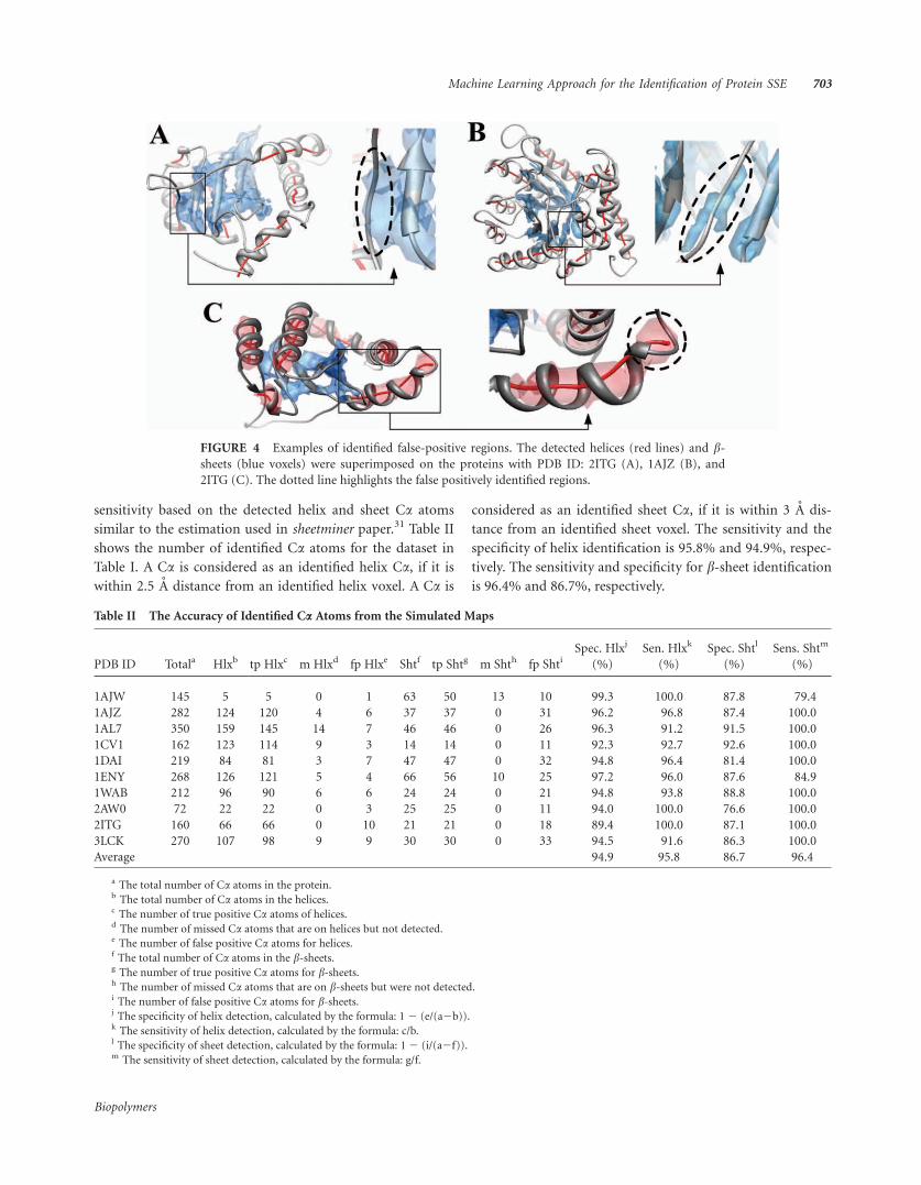
sensitivity based on the detected helix and sheet Ca atoms

similar to the estimation used in sheetminer paper.31 Table II

shows the number of identified Ca atoms for the dataset in

Table I. A Ca is considered as an identified helix Ca, if it iswithin 2.5 A distance from an identified helix voxel. A Ca is

considered as an identified sheet Ca, if it is within 3 A dis-

tance from an identified sheet voxel. The sensitivity and the

specificity of helix identification is 95.8% and 94.9%, respec-

tively. The sensitivity and specificity for b-sheet identificationis 96.4% and 86.7%, respectively.

Table II The Accuracy of Identified Ca Atoms from the Simulated Maps

PDB ID Totala Hlxb tp Hlxc m Hlxd fp Hlxe Shtf tp Shtg m Shth fp ShtiSpec. Hlxj

(%)

Sen. Hlxk

(%)

Spec. Shtl

(%)

Sens. Shtm

(%)

1AJW 145 5 5 0 1 63 50 13 10 99.3 100.0 87.8 79.4

1AJZ 282 124 120 4 6 37 37 0 31 96.2 96.8 87.4 100.0

1AL7 350 159 145 14 7 46 46 0 26 96.3 91.2 91.5 100.0

1CV1 162 123 114 9 3 14 14 0 11 92.3 92.7 92.6 100.0

1DAI 219 84 81 3 7 47 47 0 32 94.8 96.4 81.4 100.0

1ENY 268 126 121 5 4 66 56 10 25 97.2 96.0 87.6 84.9

1WAB 212 96 90 6 6 24 24 0 21 94.8 93.8 88.8 100.0

2AW0 72 22 22 0 3 25 25 0 11 94.0 100.0 76.6 100.0

2ITG 160 66 66 0 10 21 21 0 18 89.4 100.0 87.1 100.0

3LCK 270 107 98 9 9 30 30 0 33 94.5 91.6 86.3 100.0

Average 94.9 95.8 86.7 96.4

a The total number of Ca atoms in the protein.b The total number of Ca atoms in the helices.c The number of true positive Ca atoms of helices.d The number of missed Ca atoms that are on helices but not detected.e The number of false positive Ca atoms for helices.f The total number of Ca atoms in the b-sheets.g The number of true positive Ca atoms for b-sheets.h The number of missed Ca atoms that are on b-sheets but were not detected.i The number of false positive Ca atoms for b-sheets.j The specificity of helix detection, calculated by the formula: 1 2 (e/(a2b)).k The sensitivity of helix detection, calculated by the formula: c/b.l The specificity of sheet detection, calculated by the formula: 12 (i/(a2f)).m The sensitivity of sheet detection, calculated by the formula: g/f.

FIGURE 4 Examples of identified false-positive regions. The detected helices (red lines) and b-sheets (blue voxels) were superimposed on the proteins with PDB ID: 2ITG (A), 1AJZ (B), and

2ITG (C). The dotted line highlights the false positively identified regions.

Machine Learning Approach for the Identification of Protein SSE 703

Biopolymers

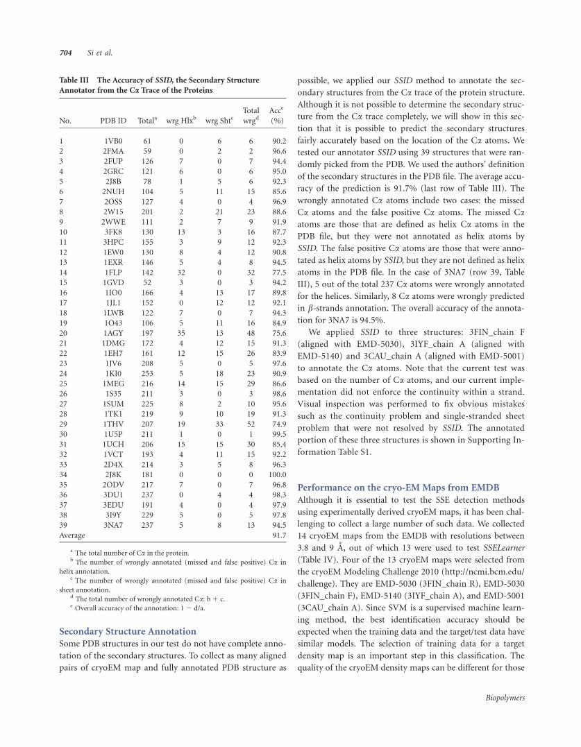
Secondary Structure Annotation

Some PDB structures in our test do not have complete anno-

tation of the secondary structures. To collect as many aligned

pairs of cryoEM map and fully annotated PDB structure as

possible, we applied our SSID method to annotate the sec-

ondary structures from the Ca trace of the protein structure.

Although it is not possible to determine the secondary struc-

ture from the Ca trace completely, we will show in this sec-

tion that it is possible to predict the secondary structures

fairly accurately based on the location of the Ca atoms. We

tested our annotator SSID using 39 structures that were ran-

domly picked from the PDB. We used the authors’ definition

of the secondary structures in the PDB file. The average accu-

racy of the prediction is 91.7% (last row of Table III). The

wrongly annotated Ca atoms include two cases: the missed

Ca atoms and the false positive Ca atoms. The missed Caatoms are those that are defined as helix Ca atoms in the

PDB file, but they were not annotated as helix atoms by

SSID. The false positive Ca atoms are those that were anno-

tated as helix atoms by SSID, but they are not defined as helix

atoms in the PDB file. In the case of 3NA7 (row 39, Table

III), 5 out of the total 237 Ca atoms were wrongly annotated

for the helices. Similarly, 8 Ca atoms were wrongly predicted

in b-strands annotation. The overall accuracy of the annota-tion for 3NA7 is 94.5%.

We applied SSID to three structures: 3FIN_chain F

(aligned with EMD-5030), 3IYF_chain A (aligned with

EMD-5140) and 3CAU_chain A (aligned with EMD-5001)

to annotate the Ca atoms. Note that the current test was

based on the number of Ca atoms, and our current imple-

mentation did not enforce the continuity within a strand.

Visual inspection was performed to fix obvious mistakes

such as the continuity problem and single-stranded sheet

problem that were not resolved by SSID. The annotated

portion of these three structures is shown in Supporting In-

formation Table S1.

Performance on the cryo-EM Maps from EMDB

Although it is essential to test the SSE detection methods

using experimentally derived cryoEM maps, it has been chal-

lenging to collect a large number of such data. We collected

14 cryoEM maps from the EMDB with resolutions between

3.8 and 9 A, out of which 13 were used to test SSELearner

(Table IV). Four of the 13 cryoEM maps were selected from

the cryoEM Modeling Challenge 2010 (http://ncmi.bcm.edu/

challenge). They are EMD-5030 (3FIN_chain R), EMD-5030

(3FIN_chain F), EMD-5140 (3IYF_chain A), and EMD-5001

(3CAU_chain A). Since SVM is a supervised machine learn-

ing method, the best identification accuracy should be

expected when the training data and the target/test data have

similar models. The selection of training data for a target

density map is an important step in this classification. The

quality of the cryoEM density maps can be different for those

Table III The Accuracy of SSID, the Secondary Structure

Annotator from the Ca Trace of the Proteins

No. PDB ID Totala wrg Hlxb wrg ShtcTotal

wrgdAcce

(%)

1 1VB0 61 0 6 6 90.2

2 2FMA 59 0 2 2 96.6

3 2FUP 126 7 0 7 94.4

4 2GRC 121 6 0 6 95.0

5 2J8B 78 1 5 6 92.3

6 2NUH 104 5 11 15 85.6

7 2OSS 127 4 0 4 96.9

8 2W15 201 2 21 23 88.6

9 2WWE 111 2 7 9 91.9

10 3FK8 130 13 3 16 87.7

11 3HPC 155 3 9 12 92.3

12 1EW0 130 8 4 12 90.8

13 1EXR 146 5 4 8 94.5

14 1FLP 142 32 0 32 77.5

15 1GVD 52 3 0 3 94.2

16 1IO0 166 4 13 17 89.8

17 1JL1 152 0 12 12 92.1

18 1LWB 122 7 0 7 94.3

19 1O43 106 5 11 16 84.9

20 1AGY 197 35 13 48 75.6

21 1DMG 172 4 12 15 91.3

22 1EH7 161 12 15 26 83.9

23 1JV6 208 5 0 5 97.6

24 1KI0 253 5 18 23 90.9

25 1MEG 216 14 15 29 86.6

26 1S35 211 3 0 3 98.6

27 1SUM 225 8 2 10 95.6

28 1TK1 219 9 10 19 91.3

29 1THV 207 19 33 52 74.9

30 1U5P 211 1 0 1 99.5

31 1UCH 206 15 15 30 85.4

32 1VCT 193 4 11 15 92.2

33 2D4X 214 3 5 8 96.3

34 2J8K 181 0 0 0 100.0

35 2ODV 217 7 0 7 96.8

36 3DU1 237 0 4 4 98.3

37 3EDU 191 4 0 4 97.9

38 3I9Y 229 5 0 5 97.8

39 3NA7 237 5 8 13 94.5

Average 91.7

a The total number of Ca in the protein.b The number of wrongly annotated (missed and false positive) Ca in

helix annotation.c The number of wrongly annotated (missed and false positive) Ca in

sheet annotation.d The total number of wrongly annotated Ca: b1 c.e Overall accuracy of the annotation: 12 d/a.

704 Si et al.

Biopolymers

at the similar resolutions. We carefully selected a training

density map for each target cryoEM map that is to be tested

(Table IV). A number of factors were taken into considera-

tion in the selection of training data. These factors include

the resolution, the estimated range of helix density, the esti-

mated range of sheet density and the estimated noise level in

the density map.

An example of the detected secondary structures is shown

in Figure 5. In this case, the cryoEM density map EMD-5030

was aligned with 3FIN_chain R. SSELearner detected all the

four helices and the b-sheet (row 1, Table V). The specificity

and the sensitivity for the detected helix Ca atoms are 93.1%

and 96.6%, and those for the sheet detection are 89.3% and

100%, respectively (row 1, Table VI).

The test of 13 cryoEM maps suggests that the helices longer

than eight amino acids and sheets with more than two strands

can be mostly detected. SSELearner detected 89 of 107 such

helices and all 26 such b-sheets (Table V). Note that SSE-

Learner detected 100% such helices and sheets in the simulated

data (Table I). The contrast shows the challenges to the SSE

detection method for the experimentally derived density maps.

This is only visible when a large number of the experimental

cryoEM density maps are used for testing. Our test also sug-

gests that SSELearner detects the b-sheets fairly well in the cry-

oEM maps. It detected all the 26 b-sheets that have more than

two strands, and 9 of 16 b-sheets with two strands (Table V).

For helices with no more than eight amino acids, SSELearner

was only able to detect 30 of 61 such helices (Table V).

We analyzed the performance of our SSE detection method

using the number of identified Ca atoms to reveal the size ac-

curacy of the SSE (Table VI). The overall specificity and sensi-

tivity are 91.8% and 74.5%, respectively, in helix detection.

The main reason for the reduced sensitivity between the simu-

lated maps verses the EMDB maps is in the short helix detec-

tion. For example, 8 out of 11 helices in EMD-1237 and 13

out of 26 helices in EMD-5100 are no more than eight amino

acids. Another reason is the reduced quality of the experimen-

tal cryoEM maps compared with that of the simulated density

maps. The experimental density maps often have incomplete

density data, particularly for the short helices. The overall

specificity and sensitivity in sheet identification are 85.2% and

86.5%, respectively. Our test using 13 experimentally derived

cryoEM maps shows the challenges in the SSE detection from

the real cryoEM maps. It is not possible to detect them as

accurately as in the simulated maps at this point.

DISCUSSIONWe have developed an approach to detect the secondary

structures from the medium resolution density maps using a

combination of image processing and supervised machine

learning techniques. The supervised machine learning allows

the input of user knowledge, and that was reflected in the

Table IV The Target CryoEM Density Maps (EMDB ID, PDB

ID, and Resolution) and Their Corresponding Training Data

Test Data Training Data

5030 (3FIN_R), 6.4 A 5168 (3MFP_A), 6.6 A

5030 (3FIN_F), 6.4 A 5168 (3MFP_A), 6.6 A

5140 (3IYF_A), 8 A 5030 (3FIN_F), 6.4 A

1733 (3C91_H), 6.8 A 1780 (3IZ6_K), 5.5 A

5168 (3MFP_A), 6.6 A 5030 (3FIN_R), 6.4 A

1237 (2GSY_A), 7.2 A 1780 (3IZ6_K), 5.5 A

5100 (3IXV_A), 6.8 A 5030 (3FIN_R), 6.4 A

5199 (3N09_C), 3.8 A 1780 (3IZ6_K), 5.5 A

1780 (3IZ6_K), 5.5 A 1740 (3C92_A), 6.8 A

5223 (3IZ0_A), 8.6 A 1340 (2P4N_A), 9 A

1340 (2P4N_A), 9 A 5223 (3IZ0_A), 8.6 A

1780 (3IZ6_T), 5.5 A 5030 (3FIN_F), 6.4 A

5001 (3CAU_A), 4.2 A 1740 (3C92_A), 6.8 A

FIGURE 5 Secondary structures detected using SSELearner. (A) Part of EMDB entry EMD-5030

at resolution 6.4 A with fitted secondary structure of protein 3FIN_chain R; (B) identified helix and

sheet locations.

Machine Learning Approach for the Identification of Protein SSE 705

Biopolymers

selection of the training density map for each target density

map. We found that this step is important for achieving good

accuracy, and it requires certain knowledge about the nature

of the density map. We visually estimated the density ranges

for helices and sheets then used such estimated parameters in

searching for the density maps for training. RENNSH demon-

strated that selecting training data from the density map

within which the test data are located is a viable approach for

the detection of a-helices.30 We extended their finding by

showing that it is possible to use different cryoEM maps for

training and test and to obtain fairly good detection accuracy.

We have demonstrated that it is possible to find a training

Table V The Identified Secondary Structures from the Experimental CryoEM Density Maps

EMDB (PDB) ID Helix\ 5aa Helix 5–8aa Helix[ 8aa Sheet 5 2 strands Sheet[ 2 strands

5030 (3FIN_R) 0/0 0/0 4/4 0/0 1/1

5030 (3FIN_F) 1/1 0/0 6/6 2/2 1/1

5140 (3IYF_A) 0/0 4/8 9/16 1/3 4/4

1733 (3C91_H) 0/0 0/0 5/5 1/1 2/2

5168 (3MFP_A) 0/0 6/9 8/10 0/1 2/2

1237 (2GSY_A) 0/3 2/5 3/3 1/1 4/4

5100 (3IXV_A) 0/2 5/11 12/13 0/1 2/2

5199 (3N09_C) 0/2 3/5 6/6 1/3 2/2

1780 (3IZ6_K) 0/0 0/1 2/2 0/0 1/1

5223 (3IZ0_A) 3/3 1/2 8/11 0/0 2/2

1340 (2P4N_A) 0/1 2/4 9/11 0/0 2/2

1780 (3IZ6_T) 0/0 0/0 4/4 1/1 0/0

5001 (3CAU_A) 0/0 3/4 13/16 2/3 3/3

Total 4/12 26/49 89/107 9/16 26/26

Table VI The Identified Ca Atoms from the Experimental cryoEM Maps

EMDB (PDB) ID Totala Hlxb tp Hlxc m Hlxd fp Hlxe Shtf tp Shtg m Shth fp ShtiSpec. Hlxj

(%)

Sen. Hlxk

(%)

Spec. Shtl

(%)

Sens. Shtm

(%)

5030 (3FIN_R) 117 59 57 2 4 14 14 0 11 93.1 96.6 89.3 100.0

5030 (3FIN_F) 208 80 71 9 4 37 37 0 15 96.9 88.8 91.2 100.0

5140 (3IYF_A) 491 263 136 127 42 74 47 27 69 81.6 51.7 83.5 63.5

1733 (3C91_H) 203 86 69 17 0 62 54 8 25 100.0 80.2 82.3 87.1

5168 (3MFP_A) 374 186 138 48 17 60 41 19 56 91.0 74.2 82.2 68.3

1237 (2GSY_A) 428 69 46 23 5 187 180 7 71 98.6 66.7 70.5 96.3

5100 (3IXV_A) 626 277 195 82 35 99 86 13 51 90.0 70.4 90.3 86.9

5199 (3N09_C) 397 144 118 26 24 128 114 14 41 90.5 81.9 84.8 89.1

1780 (3IZ6_K) 119 37 25 12 1 29 29 0 11 98.8 67.6 87.8 100.0

5223 (3IZ0_A) 412 186 116 70 34 55 42 13 24 85.0 62.4 93.3 76.4

1340 (2P4N_A) 412 202 124 78 21 55 39 16 75 90.0 61.4 79.0 70.9

1780 (3IZ6_T) 82 54 45 9 0 7 7 0 8 100.0 83.3 89.3 100.0

5001 (3CAU_A) 526 255 214 41 61 82 71 11 72 77.5 83.9 83.8 86.6

Average 91.8 74.5 85.2 86.5

a The total number of Ca atoms in the protein.b The total number of Ca atoms in the helices.c The number of true positive Ca atoms of helices.d The number of missed Ca atoms that are on helices but not detected.e The number of false positive Ca atoms for helices.f The total number of Ca atoms in the b-sheets.g The number of true positive Ca atoms for b-sheets.h The number of missed Ca atoms that are on b-sheets but were not detected.i The number of false positive Ca atoms for b-sheets.j The specificity of helix detection, calculated by the formula: 12 (e/(a2b)).k The sensitivity of helix detection, calculated by the formula: c/b.l The specificity of sheet detection, calculated by the formula: 12 (i/(a2f)).m The sensitivity of sheet detection, calculated by the formula: g/f.

706 Si et al.

Biopolymers

density map that shares similar density nature with that of the

target map in the current EMDB. We have tested using thir-

teen cryoEM density maps from the EMDB to demonstrate

that this approach is feasible. As more and more cryoEM

maps are available in the EMDB database, it is promising that

the combined image processing and machine learning techni-

ques will result in improved accuracy in SSE detection.

In principle, the resolution of the density map can affect

the accuracy of the SSE detection. We generated the density

map at 6 A (Figure 6A), 8 A (Figure 3B), and 10 A (Figure 6B)

resolution using EMAN.44 The detection of the helices appears

to be less affected by the resolution at the resolution range of

6210 A. In fact both helices were detected to similar lengths

at the three resolutions sampled (Figures 3E, 6A, and 6B). The

b-sheet was all detected at the three resolution ranges. How-

ever, the size of the detected b-sheet appears to be affected

slightly by the resolution. It appears that more true-positive

sheet voxels were detected in the 6 A density map (Figure 6A

cyan) than in the 10 A map (Figure 6B cyan).

We have developed the SSELearner for the detection of heli-

ces and b-sheets from cryoEM density maps at the medium

resolution range of 5210 A. The approach has been tested

using 10 simulated density maps as well as 13 cryoEM maps

from the EMDB. Our results show that although the detection

can be fairly accurate in the simulated density maps, the accu-

racy decreases significantly for the short helices from the

experimentally derived density maps. The specificity and the

sensitivity for the helix detection are 94.9% and 95.8%, respec-

tively, in the simulated density maps and 91.8% and 74.5% in

the experimentally derived cryoEM maps. The specificity and

the sensitivity for the b-sheet detection are 86.7% and 96.4%,

respectively, in the simulated maps and 85.2% and 86.5% in

the experimentally derived maps. The overall detection accu-

racy demonstrated that it is feasible to select a specific density

map from the current EMDB as training data to detect the

SSE of a target cryoEM map.

Secondary structure detection from the cryoEM density

map at the medium resolution is still a challenging problem

despite the multiple proposed methods. To speed-up the

research in this direction, coordinated effort is needed to

promote the public sharing of the developed software and

the development of the benchmark data that is available to

the public. However, the comparison of the software is still

challenging. Some of the methods are automatic and others

are semi-automatic.29 The continuing maintenance of the

software has also been inadequate in this area.

Old Dominion University MDS research fund and NSF DBI-1147134.

REFERENCES1. Bottcher, B.; Wynne, S. A.; Crowther, R. A. Nature 1997, 386,

88–91.

2. Mancini, E. J.; Clarke, M.; Gowen, B. E.; Rutten, T.; Fuller, S. D.

Mol Cell 2000, 5, 255–266.

3. Zhou, Z. H.; Dougherty, M.; Jakana, J.; He, J.; Rixon, F. J.; Chiu,

W. Science 2000, 288, 877–880.

4. van Heel, M.; Gowen, B.; Matadeen, R.; Orlova, E. V.; Finn, R.;

Pape, T.; Cohen, D.; Stark, H.; Schmidt, R.; Schatz, M.; Patward-

han, A. Quarterly Rev Biophys 2000, 33, 307–369.

5. Zhou, Z. H.. Curr Opin Structural Biol 2008, 18, 218–228.

6. Hryc, C. F.; Chen, D. H.; Chiu, W. Curr Opin Virol 2011, 1,

110–117.

7. Zhang, R.; Hryc, C. F.; Cong, Y.; Liu, X. G.; Jakana, J.; Gorcha-

kov, R.; Baker, M. L.; Weaver, S. C.; Chiu, W. Embo J 2011, 30,

3854–3863.

8. Settembre, E. C.; Chen, J. Z.; Dormitzer, P. R.; Grigorieff, N.;

Harrison, S. C. Embo J 2011, 30, 408–416.

9. Daban, J. R. Electron microscopy and atomic force microscopy

studies of chromatin and metaphase chromosome structure.

Micron 2011, 42, 733–750.

FIGURE 6 SSE identification at different resolutions. Protein 2AW0 (PDB ID) was used to gener-

ate the simulated density map at 6 A resolution (A) and 10 A resolution (B). The detected helix

(red line) and b-sheet (blue voxels) were superimposed on the PDB structure.

Machine Learning Approach for the Identification of Protein SSE 707

Biopolymers

10. Grigorieff, N.; Harrison, S. C. Curr Opin Struct Biol 2011, 21,

265–273.

11. Chiu, W.; Baker, M. L.; Jiang, W.; Dougherty, M.; Schmid, M. F.

Structure 2005, 13, 363–372.

12. Zhou, Z. H. Adv Protein Chem Struct Biol 2011, 82, 1–35.

13. Ludtke, S. J.; Baker, M. L.; Chen, D. H.; Song, J. L.; Chuang, D.

T.; Chiu, W. Structure 2008, 16, 441–448.

14. Jiang, W.; Baker, M. L.; Jakana, J.; Weigele, P. R.; King, J.; Chiu,

W. Nature 2008, 451, 1130–1134.

15. Yu, X.; Jin, L.; Zhou, Z. H. Nature 2008, 453, 415–419.

16. Schuette, J.-C.; Murphy, F. V.; Kelley, A. C.; Weir, J. R.; Giese-

brecht, J.; Connell, S. R.; Loerke, J.; Mielke, T.; Zhang, W.; Penc-

zek, P. A.; Ramakrishnan, V.; Spahn, C. M. T. Embo J 2009, 28,

755–765.

17. Luque, D.; Saugar, I.; Rodriguez, J. F.; Verdaguer, N.; Garriga,

D.; Martin, C. S.; Velazquez-Muriel, J. A.; Trus, B. L.; Carra-

scosa, J. L.; Caston, J. R. J Virol 2007, 81, 6869–6878.

18. Rabl, J.; Smith, D. M.; Yu, Y.; Chang, S.-C.; Goldberg, A. L.;

Cheng, Y. Molecular Cell 2008, 30, 360–368.

19. Fujii, T.; Iwane, A. H.; Yanagida, T.; Namba, K. Direct visualiza-

tion of secondary structures of F-actin by electron cryomicro-

scopy. Nature 2010, 467, 724–728.

20. Zhang, J.; Baker, M. L.; Schroder, G. F.; Douglas, N. R.; Reiss-

mann, S.; Jakana, J.; Dougherty, M.; Fu, C. J.; Levitt, M.; Ludtke,

S. J.; Frydman, J.; Chiu, W. Nature 2010, 463, 379–383.

21. Cong, Y.; Zhang, Q.; Woolford, D.; Schweikardt, T.; Khant, H.;

Dougherty, M.; Ludtke, S. J.; Chiu, W.; Decker, H. Structure

2009, 17, 749–758.

22. Sindelar, C. V.; Downing, K. H. J Cell Biol 2007, 177, 377–385.

23. Alushin, G. M.; Ramey, V. H.; Pasqualato, S.; Ball, D. A.; Grigor-

ieff, N.; Musacchio, A.; Nogales, E. Nature 2010, 467, 805–810.

24. Jiang, W.; Baker, M. L.; Ludtke, S. J.; Chiu, W. J Mol Biol 2001,

308, 1033–1044.

25. Del Palu, A.; He, J.; Pontelli, E.; Lu, Y.Proceeding of Computa-

tional Systems Bioinformatics Conference(CSB), 2006, pp 89–

98.

26. Baker, M. L.; Ju, T.; Chiu, W. Structure 2007, 15, 7–19.

27. Lasker, K.; Dror, O.; Shatsky, M.; Nussinov, R.; Wolfson, H. J.

IEEE/ACM Trans Comput Biol Bioinform 2007, 4, 28–39.

28. Zeyun, Y.; Bajaj, C. IEEE/ACM Trans Comput 2008, 5, 568–582.

29. Baker, M. L.; Abeysinghe, S. S.; Schuh, S.; Coleman, R. A.;

Abrams, A.; Marsh, M. P.; Hryc, C. F.; Ruths, T.; Chiu, W.; Ju, T.

J Structural Biol 2011, 174, 360–373.

30. Ma, L.; Reisert, M.; Burkhardt, H. Comput Biol Bioinformatics,

IEEE/ACM Trans 2011, ( 99), 1.

31. Kong, Y.; Ma, J. J Mol Biol 2003, 332, 399–413.

32. Lawson, C. L.; Baker, M. L.; Best, C.; Bi, C.; Dougherty, M.;

Feng, P.; van Ginkel, G.; Devkota, B.; Lagerstedt, I.; Ludtke, S. J.;

Newman, R. H.; Oldfield, T. J.; Rees, I.; Sahni, G.; Sala, R.;

Velankar, S.; Warren, J.; Westbrook, J. D.; Henrick, K.; Kleywegt,

G. J.; Berman, H. M.; Chiu, W. Nucleic Acids Res 2011, 39

(Database issue), D456–D464.

33. Wriggers, W.; Milligan, R. A.; McCammon, J. A. J Struct Biol

1999, 125, 185–195.

34. Topf, M.; Lasker, K.; Webb, B.; Wolfson, H.; Chiu, W.; Sali, A.

Structure 2008, 16, 295–307.

35. Schroder, G. F.; Brunger, A. T.; Levitt, M. Structure 2007, 15,

1630.

36. Fernandez, J.-J.; Li, S. J Structural Biol 2003, 144, 152–161.

37. Boser, B. E.; Guyon, I. M.; Vapnik, V. N. In Proceedings of the

Fifth Annual Workshop on Computational Learning Theory;

ACM: Pittsburgh, PA, 1992; pp 144–152.

38. Cortes, C.; Vapnik, V. Mach. Learn. 1995, 20, 273–297.

39. Chang, C.-C.; Lin, C.-J. ACM Trans Intell Syst Technol 2011, 2,

1–27.

40. Knerr, S.; Personnaz, L.; Dreyfus, G. In Neurocomputing: Algo-

rithms, Architectures and Applications; Fogelman-Soulie, F.;

Herault, J., Eds. Springer-Verlag, LLC: New York, 1990; Vol.

F68, pp 41–50.

41. Kong, Y.; Zhang, X.; Baker, T. S.; Ma, J. J Mol Biol 2004, 339,

117–130.

42. Kleywegt, G. J. J Mol Biol 1997, 273, 371–376.

43. Kabsch, W.; Sander, C. Biopolymers 1983, 22, 2577–2637.

44. Ludtke, S. J.; Baldwin, P. R.; Chiu, W. J Struct Biol 1999, 128,

82–97.

Reviewing Editor: Steven J. Ludtke

708 Si et al.

Biopolymers