An improved algorithm for anisotropic nonlinear diffusion for denoising cryo-tomograms

Journal of

Structural

Journal of Structural Biology 144 (2003) 152–161

Biology

www.elsevier.com/locate/yjsbi

An improved algorithm for anisotropic nonlinear diffusionfor denoising cryo-tomograms

Jos�ee-Jes�uus Fern�aandeza,* and Sam Lib

a Department of Computer Architecture and Electronics, University of Almer�ııa, 04120 Almer�ııa, Spainb MRC Laboratory of Molecular Biology, CB2 2QH Cambridge, UK

Received 27 May 2003, and in revised form 5 August 2003

Abstract

Cryo-electron tomography is an imaging technique with an unique potential for visualizing large complex biological specimens. It

ensures preservation of the biological material but the resulting cryotomograms are extremely noisy. Sophisticated denoising

techniques are thus essential for allowing the visualization and interpretation of the information contained in the cryotomograms.

Here a software tool based on anisotropic nonlinear diffusion is described for filtering cryotomograms. The approach reduces local

noise and meanwhile enhances both curvilinear and planar structures. In the program a novel solution of the partial differential

equation has been implemented, which allows a reliable estimation of derivatives and, furthermore, reduces computation time and

memory requirements. Several criteria have been included to automatically select the optimal stopping time. The behaviour of the

denoising approach is tested for visualizing filamentous structures in cryotomograms.

� 2003 Elsevier Inc. All rights reserved.

Keywords: Electron tomography; Denoising; Anisotropic nonlinear diffusion

1. Introduction

Cryo-electron tomography (CryoET) is a useful tool

for studying large biological specimens with a potential

resolution of a few nanometers (Baumeister et al., 1999;

Baumeister, 2002; Grunewald et al., 2003). Although it

is not a new technique (Frank, 1992), the recent devel-

opment of instruments and software has substantially

changed its applicability (for a review of the technique,

its evolution and prospects, see Frank, 1992; Kosteret al., 1997; Baumeister et al., 1999; McEwen and

Marko, 2001; Baumeister, 2002; Grunewald et al.,

2003)). The current automation of low-dose data-ac-

quisition procedures allows the study of 3D structures of

unstained biological materials in near-physiological

conditions. Therefore, it has potential to bridge the gap

between cellular and molecular structural biology, and

allows us to understand the cellular content in moleculardetails (Grunewald et al., 2003; Sali et al., 2003). Some

examples of recent applications of CryoET to the anal-

* Corresponding author. Fax: +34-950-015-486.

E-mail address: [email protected] (J.-J. Fern�aandez).

1047-8477/$ - see front matter � 2003 Elsevier Inc. All rights reserved.

doi:10.1016/j.jsb.2003.09.010

ysis of large pleiomorphic structures have been reported,

including cellular organelles (Nicastro et al., 2000;Bohm et al., 2001; Nickell et al., 2003) and whole cells

(Grimm et al., 1998; Medalia et al., 2002).

Although great effort has been made for tomographic

data collection, visualization of tomograms is cumber-

some due to (1) low-dosage and low contrast imaging

conditions, (2) limited number of projections along

single or double tilt axes, and (3) large-size specimen

embedded in thick ice (>300 nm). These result in poorsignal-to-noise ratio (SNR) and severely hinder the in-

terpretation of the tomogram. In the last instance, this

low SNR precludes the direct application of image

analysis techniques, such as automatic segmentation,

pattern recognition, and techniques to extract useful

information from the tomogram (Grunewald et al.,

2003). Therefore it is evident that sophisticated filtering

techniques are necessary before interpretation of thereconstructed tomogram (Frangakis and Hegerl, 2001;

Frangakis et al., 2001; Medalia et al., 2002).

Anisotropic nonlinear diffusion (AND) is a filtering

method that reduces noise and enhances local structure

which has been widely used in computational vision

mail to: [email protected]

J.-J. Fern�aandez, S. Li / Journal of Structural Biology 144 (2003) 152–161 153

(Weickert, 1998). It was first introduced in visualizingelectron tomograms by Frangakis and Hegerl (2001)

and Frangakis et al. (2001) and shows a superior per-

formance to other filtering methods. Here, we report the

development of a software program for filtering cryot-

omograms based on AND, which has additional im-

proved functionalities suitable for visualizing 3D

tomograms from single tilt-axis CryoET.

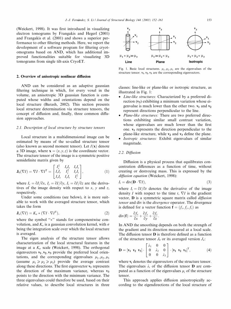
Fig. 1. Basic local structures. l1; l2;l3 are the eigenvalues of the

structure tensor. v1; v2; v3 are the corresponding eigenvectors.

2. Overview of anisotropic nonlinear diffusion

AND can be considered as an adaptive gaussian

filtering technique in which, for every voxel in the

volume, an anisotropic 3D gaussian function is com-

puted whose widths and orientations depend on the

local structure (Barash, 2002). This section presentslocal structure determination via structure tensors, the

concept of diffusion and, finally, three common diffu-

sion approaches.

2.1. Description of local structure by structure tensors

Local structure in a multidimensional image can be

estimated by means of the so-called structure tensor(also known as second moment tensor). Let IðxÞ denotea 3D image, where x ¼ ðx; y; zÞ is the coordinate vector.

The structure tensor of the image is a symmetric positive

semidefinite matrix given by

J0ðrIÞ ¼ rI � rIT ¼I2x IxIy IxIzIxIy I2y IyIzIxIz IyIz I2z

24

35; ð1Þ

where Ix ¼ oI=ox, Iy ¼ oI=oy, Iz ¼ oI=oz are the deriva-

tives of the image density with respect to x, y and z,respectively.

Under some conditions (see below), it is more suit-

able to work with the averaged structure tensor, which

takes the form

JrðrIÞ ¼ Kr � ðrI � rITÞ; ð2Þwhere the symbol ‘‘�’’ stands for componentwise con-

volution, and Kr is a gaussian convolution kernel, with rbeing the integration scale over which the local structure

is averaged.

The eigen analysis of the structure tensor allowscharacterization of the local structural features in the

image at a Kr scale (Weickert, 1998). The orthogonal

eigenvectors v1; v2; v3 provide the preferred local orien-

tations, and the corresponding eigenvalues l1; l2; l3(assume l1 P l2 P l3) provide the average contrast

along these directions. The first eigenvector v1 represents

the direction of the maximum variance, whereas v3points to the direction with the minimum variance. Thethree eigenvalues could therefore be used, based on their

relative values, to describe local structures in three

classes: line-like or plane-like or isotropic structure, as

illustrated in Fig. 1:• Line-like structures: Characterized by a preferred di-

rection (v3) exhibiting a minimum variation whose ei-

genvalue is much lower than the other two. v1 and v2represent directions perpendicular to the line.

• Plane-like structures: There are two preferred direc-

tions exhibiting similar small contrast variation,

whose eigenvalues are much lower than the first

one. v1 represents the direction perpendicular to theplane-like structure, while v2 and v3 define the plane.

• Isotropic structures: Exhibit eigenvalues of similar

magnitude.

2.2. Diffusion

Diffusion is a physical process that equilibrates con-

centration differences as a function of time, withoutcreating or destroying mass. This is expressed by the

diffusion equation (Weickert, 1998):

It ¼ divðD � rIÞ; ð3Þwhere It ¼ oI=ot denotes the derivative of the image

density I with respect to the time t, rI is the gradient

vector, D is a symmetric square matrix called diffusion

tensor and div is the divergence operator. The divergence

is defined for a vector function f ¼ ðfx; fy ; fzÞ as

divðfÞ ¼ ofxox

þ ofyoy

þ ofzoz

:

In AND the smoothing depends on both the strength of

the gradient and its direction measured at a local scale.

The diffusion tensor D is therefore defined as a function

of the structure tensor J0 or its averaged version Jr:

D ¼ ½v1 v2 v3� �k1 0 0

0 k2 0

0 0 k3

24

35 � ½v1 v2 v3�T; ð4Þ

where vi denotes the eigenvectors of the structure tensor.

The eigenvalues ki of the diffusion tensor D are com-

puted as a function of the eigenvalues li of the structure

tensor.

This approach applies diffusion anisotropically ac-

cording to the eigendirections of the local structure of

154 J.-J. Fern�aandez, S. Li / Journal of Structural Biology 144 (2003) 152–161

the image. The strength of the diffusion along them isbased on the corresponding eigenvalues ki of D.

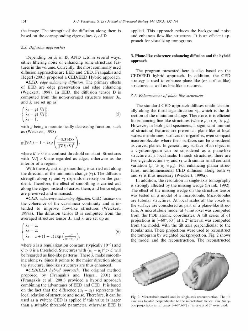
Fig. 2. Microtubule model and its single-axis reconstruction. The tilt

axis was located perpendicular to the microtubule helical axis. Sixty-

one projections in tilt range ½�60�; 60�� at intervals of 2� were used.

2.3. Diffusion approaches

Depending on ki in D, AND acts in several ways,

either filtering noise or enhancing some structural fea-

tures in the volume. Currently, the most commonly used

diffusion approaches are EED and CED. Frangakis andHegerl (2001) proposed a CED/EED Hybrid approach.

dEED: edge enhancing diffusion. The primary effects

of EED are edge preservation and edge enhancing

(Weickert, 1998). In EED, the diffusion tensor D is

computed from the non-averaged structure tensor J0,

and ki are set up as

k1 ¼ gðjrI jÞ;k2 ¼ gðjrI jÞ;k3 ¼ 1;

8<: ð5Þ

with g being a monotonically decreasing function, suchas (Weickert, 1998)

gðjrI jÞ ¼ 1� exp�3:31488

ðjrI j=KÞ8

!;

where K > 0 is a contrast threshold constant; Structures

with jrI j > K are regarded as edges, otherwise as the

interior of a region.With these ki, a strong smoothing is carried out along

the direction of the minimum change (v3). The diffusion

strength along v1 and v2 depends inversely on the gra-

dient. Therefore, the effect of smoothing is carried out

along the edges, instead of across them, and hence edges

are preserved and enhanced.dCED: coherence enhancing diffusion. CED focuses on

the coherence of the curvilinear continuity and is in-tended to improve flow-like structures (Weickert,

1999a). The diffusion tensor D is computed from the

averaged structure tensor Jr and ki are set up as

k1 ¼ a;k2 ¼ a;

k3 ¼ aþ ð1� aÞ exp �Cðl1�l3Þ2

� �;

8><>: ð6Þ

where a is a regularization constant (typically 10�3) and

C > 0 is a threshold. Structures with ðl1 � l3Þ2> C will

be regarded as line-like patterns. These ki make smooth-

ing along v3. Since it points to the major direction along

the structure, line-like structures are thus enhanced.dCED/EED hybrid approach. The original method

proposed by (Frangakis and Hegerl, 2001) and

(Frangakis et al., 2001) provided a hybrid approachcombining the advantages of EED and CED. It is based

on the fact that the difference ðl1 � l3Þ represents the

local relation of structure and noise. Therefore, it can be

used as a switch: CED is applied if this value is larger

than a suitable threshold parameter, otherwise EED is

applied. This approach reduces the background noiseand enhances flow-like structures. It is an efficient ap-

proach for visualizing tomograms.

3. Plane-like coherence enhancing diffusion and the hybrid

approach

The program presented here is also based on theCED/EED hybrid approach. In addition, the CED

strategy is used to enhance plane-like (or surface-like)

structures as well as line-like structures.

3.1. Enhancement of plane-like structures

The standard CED approach diffuses unidimension-

ally along the third eigendirection v3, which is the di-rection of the minimum change. Therefore, it is efficient

for enhancing line-like structures (where l1 � l2 � l3).However, in biological specimens, a significant amount

of structural features are present as plane-like at local

scales: membranes, surfaces of organelles, even compact

macromolecules where their surfaces can be considered

as curved planes. In general, any surface of an object in

a cryotomogram can be considered as a plane-likestructure at a local scale. In such structures, there are

two eigendirections v2 and v3 with similar small contrast

variation (l1 � l2 � l3). For enhancing planar struc-

tures, multidimensional CED diffusion along both v2and v3 is thus necessary (Weickert, 1999a).

In addition, the resolution in single-axis tomography

is strongly affected by the missing wedge (Frank, 1992).

The effect of the missing wedge on the structure tensorwas tested on a model of a microtubule. Microtubules

are tubular structures. At local scales all the voxels in

the surface are considered as part of a plane-like struc-

ture. A microtubule model at 4 nm/voxel was computed

from the PDB atomic coordinates. A tilt series of 61

projections in ½�60�; 60�� at a 2� interval was computed

from the model, with the tilt axis perpendicular to the

tubular axis. These projections were used to reconstructthe tomogram by weighted backprojection. Fig. 2 shows

the model and the reconstruction. The reconstructed


microtubule appears as two parallel walls instead of ahollow cylindrical structure.

To quantify the effect of the missing wedge, the angle

between the Z-axis and the eigenvectors was computed

for all the surface-like voxels in the model and the re-

construction. The range of possible values for the angle

between the Z-axis and the eigenvectors (½0�; 90��) wasdiscretized into nine bins (see Fig. 3A). The first bin

represents the range of ½0�; 10�� with respect to theZ-axis, which is the bin closest to the direction of the Z-axis. The last bin represents the range ½80�; 90��, i.e. theclosest to the XY plane and the farthest from the Z-axis.

Fig. 3B shows the histograms (in %) of the distribu-

tion of the angle between Z-axis and the three

eigenvectors for the microtubule model and the recon-

struction. Abscissa represents the angle with respect to

the Z-axis, discretized into the nine bins. In the originalmodel, v1, which is perpendicular to the microtubule

surfaces, is distributed throughout the range nearly

uniformly. v3 is clearly located on the XY plane, parallel

to the tubular axis. However, the histograms of the

single-axis reconstruction change substantially. v1 is in-

stead predominantly located on the XY plane, which

indicates that the reconstruction is made up of walls or

planes perpendicular to the XY plane. v3 is in turn dis-tributed throughout the angle range.

These results show that, due to the missing wedge,

structure tensors in the tomogram have a tendency with

the first eigendirection v1 going downwards (towards the

plane XY ) and v3 upwards (towards Z). The second ei-

genvector is also affected, but the new direction is not so

relevant since it is given by the other eigenvectors, as all

of them must be orthogonal. In this work, other models(a hollow sphere and planes in different directions) and

other orientations of the single tilt axis have been tested.

Similar effects of the missing wedge have been observed

(data not shown).

Fig. 3. (A) The angle between the Z-axis and the eigenvectors is discretized

eigenvectors of the microtubule model. On the left, the histograms for the

struction.

The tests that were carried out indicate that, in single-axis tomography, the eigendirections measured from the

tomograms are severely distorted compared to the

directions in the original specimen. In the case of plane-

like structures, if the diffusion were restricted along the

third eigenvector v3, it would then be driven only by one

of the vectors defining the plane. Moreover, v3 may

misrepresent the feature because of the distortion. In

these cases, the diffusion should involve v2 and v3. Al-though distorted, the combined information provided

by both is valuable to find out the planar information.

Therefore, diffusion using second and third eigendirec-

tions is essential for successfully denoising and enhanc-

ing plane-like structures, and the improvement is more

significant as stronger effects due to the missing wedge is

present in the reconstruction.

3.2. Detection of plane-like structures

In practice, a reconstructed tomogram contains both

plane-like and line-like structures. Therefore, it is nec-

essary to develop a mechanism to discern these features

and meanwhile, to avoid artifacts when applying CED.

In this work, we have defined a set of metrics to es-

timate whether the features are plane-like, line-like orisotropic. Let P1, P2, and P3 be the following metrics:

P1 ¼ l1�l2l1

P2 ¼ l2�l3l1

P3 ¼ l3l1

which satisfy 06 Pi 6 1, 8i and P1 þ P2 þ P3 ¼ 1, and

where l1, l2, and l3 are the eigenvalues of the averaged

structure tensor Jr.These metrics P1, P2, and P3 provide, respectively,

measures about the planar, linear or isotropic nature of

the local structure. A voxel is said to be part of one of

those structures according to the following conditions:

into 9 bins. (B) Histograms of the angle between Z-axis and the three

original model. On the right, the histogram for the single-axis recon-


P1 > P2 and P1 > P3 ) plane-like;

P2 > P1 and P2 > P3 ) line-like;

P3 > P1 and P3 > P2 ) isotropic:

These metrics allow the diffusion method to proceed

safely without producing artifacts in the structures. CEDalong second and third eigendirections is only applied for

voxels classified as part of plane-like structures.

3.3. The final diffusion approach

The following is the outline of our approach for

AND:

1. Determination EED vs CED. This step is intended todetermine if the voxel is to be processed as EED or

CED. The voxel is considered CED if the local rela-

tion of structure and noise, given by l1 � l3 from

J0, is larger than a suitable threshold. Otherwise,

the voxel is considered EED. The threshold is com-

puted from the mean value of ðl1 � l3Þ in a subvo-

lume of the image containing only noise. This

subvolume is previously delimited by the user.2. EED: edge enhancing diffusion. If the voxel is classi-

fied as EED, the diffusion tensor D (see Eq. (4)) is

computed from the non-averaged structure tensor

J0, and ki are set up according to Eq. (5).

3. CED: coherence enhancing diffusion. If the voxel is

classified as CED, the steps to follow are:

3.1.Determination if planar local structure. The voxel

is considered part of a plane-like structure if theconditions in Section 3.2 are met.

3.2.Planar enhancing diffusion. If it does belong to a

plane, the diffusion tensor D is computed from

the averaged structure tensor Jr, and ki are set

up to allow diffusion along the second and third

eigendirections:

k1 ¼ a;

k2 ¼ aþ ð1� aÞ exp �C2

ðl1�l2Þ2

� �;

k3 ¼ aþ ð1� aÞ exp �C3

ðl1�l3Þ2

� �:

8>><>>:3.3.Curvilinear enhancing diffusion. Otherwise, the

standard CED is applied. D is computed from

Jr, and ki are set up to diffuse only along the third

eigendirection according to Eq. (6).

4. Implementation

4.1. Discretization scheme

In this work, a novel discretization scheme is pro-

posed for AND in three dimensions. It is based on Euler

forward explicit numerical schemes and uses derivative

filters to approximate the spatial derivatives in the dif-

fusion formulae.

The diffusion equation (Eq. (3)) can be numericallysolved using finite differences. The term It ¼ oI=ot can be

replaced by an Euler forward difference approximation.

The resulting explicit scheme allows calculation of the

image at a new time step directly from the version at the

previous step:

I ðkþ1Þ ¼ I ðkÞ þ s � o

oxðD11IxÞ

�þ o

oxðD12IyÞ þ

o

oxðD13IzÞ

þ o

oyðD21IxÞ þ

o

oyðD22IyÞ þ

o

oyðD23IzÞ

þ o

ozðD31IxÞ þ

o

ozðD32IyÞ þ

o

ozðD33IzÞ

�; ð7Þ

where s denotes the time step size, I ðkÞ denotes the image

at time tk ¼ ks and Ix ¼ oI=ox, Iy ¼ oI=oy, and

Iz ¼ oI=oz are the derivatives of the image density with

respect to x, y, and z, respectively. The Dmn terms rep-resent the components of the diffusion tensor D.

The standard explicit numerical scheme (Weickert,

1998) for solving the partial differential equation (PDE)

in Eq. (7) is based on central differences to approximate

the spatial derivatives (o=ox, o=oy, and o=oz). The

standard approach then involves a 3� 3� 3-stencil in

solving the PDE.

In this work, the spatial derivatives have been ap-proximated by derivative filters that have been proved to

be optimal (Jahne et al., 1999). These filters approximate

rotational invariance significantly better than traditional

kernels (Weickert and Scharr, 2002).

In order to provide the AND approach with better

capabilities for structural preservation, a 3D version of

these rotational-invariant filters has been derived (see

Appendix A for details of the derivation). The use ofthese 3� 3� 3 filters results in a more reliable approxi-

mation of the derivatives. Furthermore, it involves a

5� 5� 5-stencil in the solution of the PDE. Finally, the

rotational invariance allows preservation of finer details

because the gradients account for curvatures in the

structures (Weickert and Scharr, 2002).

4.2. Efficiency of the discretization scheme

The explicit numerical scheme based on 3D rota-

tionally invariant kernels for the spatial derivatives has

been proved (Weickert and Scharr, 2002) to allow a four

times larger time step size (s ¼ 0:4) than the traditional

explicit scheme (s ¼ 0:1). This is due to the use of larger

stencils in the PDE solution, which makes the discreti-

zation scheme more stable. Consequently, the programpresented here requires 4 times less iterations than the

traditional scheme.

However, the scheme based on a 5� 5� 5-stencil is

more computationally complex and every iteration takes

more time than the traditional scheme. At the end, our

implementation exhibits a net speedup of the AND


method by about 1.5–3.0 compared to the traditionalscheme.

4.3. Memory requirements

Denoising based on AND combining the EED and

CED approaches has huge memory requirements.

Structure tensors, input and output volumes, and some

other additional matrices are needed, which makes themethod require up to 15 times the size of the input volume.

Our implementation has optimized memory usage. It

uses only one copy of the matrix for the structure ten-

sors. Since a given voxel is processed either as EED or

CED, it is possible to combine both tensors J0ðrIÞ andJrðrIÞ in the same matrix. However, an additional

matrix which only requires one bit per voxel is then

needed to indicate if a voxel is to be processed as EEDor CED. This matrix has a negligible size compared to

the input volume. Furthermore, the gradient modulus

jrI j required for EED voxels is generated on-the-fly

from the combined structure tensor (see Eq. (1)) since

jrI j ¼ I2x þ I2y þ I2z .Consequently, memory requirements here are eight

times the size of the input volume: two for the volumes in

the current and previous iterations and six for the struc-ture tensors. An additional relatively small bit-matrix

storing the CED/EED information is also required.

It would be possible to further reduce the memory

requirements for the structure tensors to a minimum at

expenses of computation time. By using a sliding win-

dow of 5� 5� 5, the structure tensors could also be

computed on-the-fly. However, the penalty in compu-

tation time might be significant.

4.4. The algorithm of the diffusion approach

The algorithm for solving the PDE in Eq. (7) using

the discretization of the temporal and spatial derivatives

described above consists of the following steps:

1. Compute the structure tensor combining J0 and Jr.

2. Compute the diffusion tensor D from the correspond-ing entries of J0 or Jr, according to the strategy de-

scribed in Section 3.3.

3. Compute the resulting image at the current step kfrom the previous step k � 1 by means of Eq. (7).

The resulting image corresponds to the diffusion time

tk ¼ ks.This algorithm is executed iteratively for a number of

iterations N . The final image is the result after a totaldiffusion time T ¼ tN ¼ Ns.

5. Stopping criterion

AND is an iterative denoising method which pro-

duces successive filtered versions of the image (see Eq.

(7)). A crucial question is when to stop the filteringprocess, so that the signal in the image is not signifi-

cantly affected by the denoising. Several objective stop-

ping criteria have been proposed (see (Mrazek and

Navara, 2003) for a brief review). In this work, some of

them have been implemented and tested.

The first stopping approach (Weickert, 1999b) is

based on the fact that the relative variance (ratio be-

tween the variances of the filtered image at time t, I t, andthe original noisy image I0) decreases monotonically

from 1 to 0 during diffusion. A stopping criterion may

be defined by a threshold over the relative variance. A

suitable threshold is also proposed based on a-priori

knowledge on the variance of the noise (Weickert,

1999b). However, in most cases this threshold underes-

timates the optimal stopping time (Mrazek and Navara,

2003). Therefore, a threshold based on the desired re-duction factor of the variance with respect to that of the

original image is more appropriate. For instance, a

threshold of 0.4 would mean that the denoising process

should stop when the image I t exhibits less than 0:4� the

variance of the input image I0. The formula of relative

variance is given by

rðtÞ ¼ varðI tÞvarðI0Þ :

The second criterion, Decorrelation criterion (Mrazek

and Navara, 2003), assumes that signal and noise are

uncorrelated. It is based on the correlation between thefiltered image at time t, I t, and the noise. The noise is

estimated as the difference between the original noisy

image I0 and the current filtered version, I t. This cor-

relation should decrease, meaning that the noise that

was eliminated and the signal are not correlated. How-

ever, if that correlation increases, which indicates the

signal is starting being affected, then the diffusion has to

be stopped. This criterion defines optimal stopping timeat minimum of the correlation coefficient between the

estimates of the noise and signal

tstop ¼ argmintjcorrðI0 � I t; I tÞj:The decorrelation criterion estimates the optimal diffu-

sion stopping time without any a-priori knowledge on

the signal and noise. However, this criterion is notguaranteed to be unimodal nor exhibits a single mini-

mum (Mrazek and Navara, 2003). In some applications

the first local minimum coincides with the global one

and thus the criterion is still valid (Mrazek and Navara,

2003). Our experience of using this criterion is that, in

general, it exhibits non-unimodal tendencies and thus is

not reliable for defining a suitable time to stop the fil-

tering.Finally, we propose a stopping criterion based on the

evolution of the variance in the subvolume of noise from

which the threshold for the EED/CED switch is also

computed (see Section 3.3). The relative noise variance is


the ratio between the variance of the noise subvolumeat time t, I tN , and the variance of the original subvo-

lume, I0N :

rN ðtÞ ¼var I tN� �

varðI0N Þ:

This curve decreases monotonically from 1 to 0 and, as

for the relative variance. A stopping criterion may thenbe established by defining a suitable threshold based on

the desired noise reduction factor. For example, a

threshold of 0:1 would mean that the denoising process

should stop when the remaining variance in the noise

subvolume I tN is less than 0:1� the variance of the sub-

volume in the input image I0N .

6. Application

As an illustration, the results from the application of

AND to tomograms of microtubules embedded in ice

are presented and discussed. The tomogram was re-

constructed through weighted backprojection of a tilt

series from ½�60�; 60��, at 1.5� interval. The images were

recorded with an FEI Tecnai F30 TEM at 300 kV. Thereconstructed tomogram was finally downsampled to

4.0 nm/voxel.

The tomogram was filtered using AND with the fea-

tures described in the previous sections. In order to

compare the plane-enhancing CED described in Section

3, the denoising was carried out using EED combined

with (1) plane-enhancing CED (diffusion along v2 and v3)

according to Section 3.3 and (2) only curvilinear-en-hancing CED (diffusion along v3). In both cases, the pa-

rameters for K for EED, and C for CED were the same.

Fig. 4 shows the curves of the three stopping criteria

tested here. On the left, the curves of the relative vari-

ance (RV) and the relative noise variance (RNV) are

shown. On the right, the curves for the correlation co-

efficient between the estimates of noise and signal in the

Fig. 4. Convergence curves corresponding to the different stopping criteria.

orrelation criterion.

decorrelation criterion are shown. RNV exhibits thesame curve for both cases and thus they overlap. Ac-

cording to RV, plane-enhancing CED is clearly better

since from the beginning the variance decrease is larger.

With regard to the decorrelation criterion on the right,

the correlation curve exhibits a single minimum for

curvilinear-enhancing CED, whilst its tendency is far

from unimodal for plane-enhancing CED.

The AND denoising process was stopped at the sev-enth iteration, equivalent to a time step of t ¼ 2:8, whereRNV reaches 0.1. RV in turn exhibits at that iteration a

value below 0.4 in the case of plane-enhancing CED,

whereas curvilinear-enhancing CED needs 25 iterations

to reach similar values of RV. The result of curvilinear-

enhancing CED at 25 iterations (not shown here)

exhibits a more homogeneous background, but no sig-

nificant improvement in the CED areas, i.e. the reduc-tion of variance is mainly due to noise reduction.

According to the decorrelation criterion, the diffusion

should also stop at the seventh iteration in the case of

curvilinear-enhancing CED, since the minimum of the

curve is located there. However, in the case of plane-

enhancing CED, the correlation does not exhibit a curve

with a well defined stopping time. Nevertheless, it seems

that around the seventh iteration this curve shows asubstantial change of slope that might be considered as

an indication.

Fig. 5 shows the denoising results for a slice of the

tomogram. The noise filtering with respect to the origi-

nal slice is evident in both denoising cases. However, the

enhancing and smoothing of the microtubules are more

apparent in the case of plane-enhancing CED. The

continuity of the microtubules is now significant. Notonly do the microtubules look much better, but the area

just around them is also further smoothed, allowing a

better definition of their boundaries. However, the result

from curvilinear-enhancing CED does not exhibit a

significant enhancement of the microtubules with re-

spect to the original slice.

Left: relative variance and relative noise variance criteria. Right: dec-

Fig. 5. Denoising with AND using EED and CED. From top to

bottom: the original slice; denoised version with EED combined with

plane-enhancing CED; denoised version with EED combined

with curvilinear-enhancing CED. K for EED, C for CED and time step

were set up to 0.018, 5� 10�8, and 2.8, respectively. The visualized

density range is l� 4 � r, where l and r are the mean and standard

deviation of the corresponding tomogram. The tilt axis is along the

vertical direction.

Fig. 6. Isosurface representation of a part of amicrotubule. From top

to bottom: the original microtubule area; denoised version with EED

combined with plane-enhancing CED; denoised version with EED

combined with curvilinear-enhancing.


Fig. 6 shows the results of the isosurface representa-

tion of a part of a microtubule in the tomogram.

Clearly, the original tomogram looks very noisy, and

denoising significantly improves the visualization of the

microtubule. Both denoising approaches yield results

much cleaner than the original. The effect of the missingwedge is evident in the pictures. The microtubule looks

like a couple of parallel walls instead of a tubular

structure. The microtubule resulting from the plane-

enhancing CED exhibits more continuity along the

walls, without disruptions. However, the result from

curvilinear-enhancing CED is not so continuous, and

still contains some disruptions and small artifacts along

the microtubule.

7. Discussion and conclusion

Filtering techniques are necessary to allow visuali-

zation and interpretation of the information about the

supramolecular organization of biological specimens

obtained from CryoET. In this paper a software tool for

filtering cryotomograms based on AND has been de-

scribed. The approach is based on the hybrid EED/CED

denoising approach first introduced by Frangakis and

Hegerl (2001). The program described here contains anumber of improvements, including recent advances in

computer vision.

First, the program includes a new diffusion mode,

plane-enhancing CED, which enhances surface-like or

plane-like local structures in tomograms. This CED

mode turns out to be useful in general, as tomograms

normally exhibit a significant amount of such structural

features. This work has shown a quantitative analysis ofthe effects of the missing wedge in single-axis tomogra-

phy on the distorting change in the eigenvectors of the

local structures. The use of plane-enhancing CED allows

a better enhancement of the distorted surface- or plane-

like local structures. This improvement has been shown


for the particular example of cryotomograms of micro-tubules, where the distorting effect of the missing wedge

may be particularly dramatic.

The software tool uses a novel discretization scheme

that has been derived to solve the partial differential

equation in the diffusion process. Compared to the stan-

dard numerical scheme, this one is more reliable for

computing derivatives and exhibits better rotational in-

variance. One of the direct consequences of this scheme isthe stability in the PDE solution. This results in a reduc-

tion of the number of iterations by a factor of 4, and a net

speedup by about 1.5–3.0, depending on the computer.

The program also reduces the memory requirements.

Previously, the hybrid EED/CED approach required up

to 15 times the size of the input tomogram. The present

tool needs eight times the size of the tomogram plus a

relatively small auxiliary matrix. As an example of thememory needs, denoising a tomogram of 100 Mbytes in

size would require around 803MB, compared to about

1.5GB previously.

Finally, the program provides a set of stopping cri-

teria. The relative variance and relative noise variance

seem to be the most useful ones. The former takes into

account the entire tomogram to compute the metric,

whereas the latter considers only a noise subvolume. Bydefining a threshold over those metrics, it is possible to

find an optimal stopping time of the diffusion process.

The thresholds should be set according to the desired

variance reduction. In this work, it was seen that

thresholds around 0.4 for the relative variance and 0.1

for the relative noise variance are reasonable.

The decorrelation criterion turns out to be of limited

applicability. It is based on the unimodality of the curve,but the curves from the tomograms in this work have

proved to be, in general, monotonically decreasing.

Consequently, it has been difficult to apply this criterion

in practice. This could be due to the combined use of

EED and CED. The criterion was introduced for linear

and nonlinear diffusion and might not be suitable for

EED/CED hybrid anisotropic diffusion. Further work is

needed to stablish an objective criterion which takes intoconsideration both the variance reduction and the signal

enhancement for estimating a suitable stopping diffusion

time. Such a criterion would stop the diffusion in the

time step when the signal starts being affected, for ex-

ample, by too much CED, thus smearing out interesting

structural features.

Acknowledgments

The author wishes to thank Drs. Frangakis and He-

gerl for kindly providing the code of AND, Dr. R.A.

Crowther for critical reading the manuscript and their

support and help throughout the work, and Drs. R.

Henderson, A.M. Roseman and P.B. Rosenthal for

helpful discussions. This work has been partially devel-oped while JJF was visiting the MRC Laboratory of

Molecular Biology. SL is supported by a HFSP long-

term fellowship. This work has been supported by the

MRC (UK) and the Spanish CICYT grant TIC2002-

00228.

Appendix A. Derivation of kernels for computing spatial

derivatives with optimally directional invariance

The spatial derivatives in the diffusion formulae have

been approximated by derivative filters with optimally

directional invariance. The 3D version of the filter has

been derived by using the techniques described in (Jahne

et al., 1999). In essence, the filter is derived by the

convolution of a 1D derivative kernel (½�1; 0; 1�=2, de-noted by D) and 1D smoothing kernels (denoted by B)in all other directions. The optimal value of B for a3� 3� 3 derivative filter was found to be: [0.174654,

0.650692, 0.174654] (see (Jahne et al., 1999) for details).

The kernels to approximate the derivatives are thus

computed as

o

ox¼ Dx � By � Bz;

o

oy¼ Dy � Bz � Bx;

o

oz¼ Dz � Bx � By ;

where the subscripts x; y; z in D and B represent the di-rection of the kernel, and � is a convolution. That way,

the 3� 3� 3 kernel used for computing the derivative

o=ox (the kernels for o=oy and o=oz are computed sim-

ilarly) results in

1

2

�0:0305 0 0:0305�0:1136 0 0:1136�0:0305 0 0:0305

24

35 �0:1136 0 0:1136

�0:4234 0 0:4234�0:1136 0 0:1136

24

35 �0:0305 0 0:0305

�0:1136 0 0:1136�0:0305 0 0:0305

24

35:

References

Barash, D., 2002. A fundamental relationship between bilateral

filtering, adaptive smoothing and the nonlinear diffusion equation.

IEEE Trans. Pattern Anal. Mach. Intel. 24, 844–847.

Baumeister, W., 2002. Electron tomography: towards visualizing the

molecular organization of the cytoplasm. Curr. Opin. Struct. Biol.

12, 679–684.

Baumeister, W., Grimm, R., Walz, J., 1999. Electron tomography of

molecules and cells. Trends Cell Biol. 9, 81–85.

Bohm, J., Lambert, O., Frangakis, A., Letellier, L., Baumeister, W.,

Rigaud, J., 2001. FhuA-mediated phage genome transfer into

liposomes. A cryo-electron tomography study. Curr. Biol. 11,

1168–1175.

Frangakis, A., Hegerl, R., 2001. Noise reduction in electron tomo-

graphic reconstructions using nonlinear anisotropic diffusion. J.

Struct. Biol. 135, 239–250.


Frangakis, A., Stoschek, A., Hegerl, R., 2001. Wavelet transform

filtering and nonlinear anisotropic diffusion assessed for signal

reconstruction performance on multidimensional biomedical data.

IEEE Trans. Biomed. Eng. 48, 213–222.

Frank, J. (Ed.), 1992. Electron Tomography. Three-Dimensional

Imaging with the Transmission Electron Microscope. Plenum

Press, New York.

Grimm, R., Singh, H., Rachel, R., Typke, D., Zillig, W., Baumeister,

W., 1998. Electron tomography of ice-embedded prokaryotic cells.

Biophys. J. 74, 1031–1042.

Grunewald, K., Medalia, O., Gross, A., Steven, A., Baumeister, W.,

2003. Prospects of electron cryotomography to visualize macro-

molecular complexes inside cellular compartments: implications of

crowding. Biophys. Chem. 100, 577–591.

Jahne, B., Scharr, H., Korkel, S., 1999. In: Jhne, B., Hauecker, H.,

Geile, P. (Eds.), Handbook of Computer Vision and Applications,

Vol. 2: Signal Processing and Pattern Recognition. Academic Press,

San Diego, pp. 125–152 (Chapter: Principles of Filter Design).

Koster, A., Grimm, R., Typke, D., Hegerl, R., Stoschek, A., Walz, J.,

Baumeister, W., 1997. Perspectives of molecular and cellular

electron tomography. J. Struct. Biol. 120, 276–308.

McEwen, B., Marko, M., 2001. The emergence of electron tomography

as an important tool for investigating cellular ultrastructure. J.

Histochem. Cytochem. 49, 553–564.

Medalia, O., Weber, I., Frangakis, A., Nicastro, D., Gerisch, G.,

Baumeister, W., 2002. Macromolecular architecture in eukaryotic

cells visualized by cryoelectron tomography. Science 298, 1209–

1213.

Mrazek, P., Navara, M., 2003. Selection of optimal stopping time for

nonlinear diffusion filtering. Int. J. Comput. Vision 52, 189–203.

Nicastro, D., Frangakis, A., Typke, D., Baumeister, W., 2000. Cryo-

electron tomography of neurospora mitochondria. J. Struct. Biol.

129, 48–56.

Nickell, S., Hegerl, R., Baumeister, W., Rachel, R., 2003. Pyrodictium

cannulae enter the periplasmic space but do not enter the

cytoplasm, as revealed by cryo-electron tomography. J. Struct.

Biol. 141, 34–42.

Sali, A., Glaeser, R., Earnest, T., Baumeister, W., 2003. From words to

literature in structural proteomics. Nature 422, 216–225.

Weickert, J., 1998. Anisotropic Diffusion in Image Processing,

Teubner.

Weickert, J., 1999a. Coherence-enhancing diffusion filtering. Int. J.

Comput. Vision 31, 111–127.

Weickert, J., 1999b. Coherence-enhancing diffusion of colour images.

Image Vision Comput. 17, 201–212.

Weickert, J., Scharr, H., 2002. A scheme for coherence-enhancing

diffusion filtering with optimized rotation invariance. J. Visual

Commun. Image. Represent. 13, 103–118.

An improved algorithm for anisotropic nonlinear diffusion for denoising cryo-tomograms

Documents

Transcript of An improved algorithm for anisotropic nonlinear diffusion for denoising cryo-tomograms