A Holonic Architecture for the Global Automated ...

A Holonic Architecture for the Global Automated Transportation

System (GATS) Chris H.J. Beckers

Version 18 September 2008

Abstract

High costs of congestion and collisions have triggered the research into completely

automated transportation systems. The GAT system differentiates itself by its holonic

architecture. In the simplified situation where there is just one vehicle and a

deterministic system, we propose an algorithm for this architecture that can create a

point-to-point shortest path. Because of the special features of the holonic architecture

we use the proven label-correcting algorithm of Pallottino and decrease the number of

areas searched by an A* search like approach. The result is a flexible algorithm that is

scalable to as many hierarchical levels as needed, thus usable for small as well as

extended areas.

- 2 -

Index

ABSTRACT................................................................................................................................... 1

INDEX ......................................................................................................................................... 2

1. INTRODUCTION ...................................................................................................................... 3

1.1. THE GLOBAL AUTOMATED TRANSPORTATION SYSTEM ....................................................................... 3 1.2. RESULTS OF PREVIOUS STUDIES ..................................................................................................... 5 1.3. RESEARCH QUESTIONS ................................................................................................................. 5

2. THEORETICAL BACKGROUND .................................................................................................. 8

2.1. SHORTEST PATH PROBLEMS .......................................................................................................... 8 2.1.1. Static Shortest Path Approaches .................................................................................... 9 2.1.2. Dynamic Shortest Path Approaches ............................................................................. 16

2.2. SORTING PROBLEMS .................................................................................................................. 22

3. ALGORITHM FORMULATION ................................................................................................. 26

3.1. A MULTI-AGENT ENGINEERING FRAMEWORK ................................................................................ 26 3.2. TRANSPORTATION SYSTEM REQUIREMENTS ................................................................................... 27 3.3. TRANSPORTATION SYSTEM GOALS ............................................................................................... 27 3.4. A DETAILED TRANSPORTATION SYSTEM DESCRIPTION ...................................................................... 28 3.5. INFORMATION FLOWS IN THE TRANSPORTATION SYSTEM .................................................................. 33 3.6. ACTORS IN THE TRANSPORTATION SYSTEM .................................................................................... 33 3.7. SPECIFIC ALGORITHM TASKS AND PROCEDURES .............................................................................. 34

4. EVALUATION OF THE ALGORITHM AND TOOL-DESIGN ......................................................... 51

4.1. TOOL FOR THE GAT SYSTEM ....................................................................................................... 51 4.2. EXAMPLE OF THE ALGORITHM IN THE DEVELOPED TOOL ................................................................... 53 4.3. COMPARING THE ALGORITHM TO THE OPTIMAL SOLUTION ............................................................... 62

5. TOWARDS A DYNAMIC ALGORITHM ..................................................................................... 67

REFERENCES ............................................................................................................................. 71

APPENDICES ............................................................................................................................. 75

A. MASE FRAMEWORK .................................................................................................................... 75 B. STATIC DISTRIBUTED ALGORITHM GOALS ......................................................................................... 76 C. STATIC DISTRIBUTED ALGORITHM SEQUENCE DIAGRAMS..................................................................... 77 D. STATIC DISTRIBUTED ALGORITHM CLASSES ....................................................................................... 78 E. STATIC DISTRIBUTED ALGORITHM TASKS .......................................................................................... 79

- 3 -

1. Introduction

The annual costs resulting of errors and accidents in traffic are estimated to be over

$1000 per person (Cambridge Systematics, Inc., 2008). Combined with the high costs of

congestion, estimated at $430 per person per year, this has lead to the development of

automated transport systems (Zelinkovsky, 1994). The Global Automated Transportation

System (GATS) is such a system, which uses advanced algorithms to guide vehicles to

their destination and reschedule routes in case of unforeseen events. This study

contributes to the development of these algorithms.

1.1. The Global Automated Transportation System

The Global Automated Transport System aims to provide an automated, driver-less,

road-vehicle transport system, which optimizes travel, in terms of speed, safety and

economy (Zelinkovsky, 1994). The GAT system can do this better than when current

systems would be expanded, because of the new technology and architectural design. In

this section we will describe these new factors that give the GATS its competitive

advantage.

The basis lies in the communication between the vehicle and the system. The vehicles

are controlled by objects called Road-Units (RUs), that lie in an intelligent cable about

10-15 centimetres below the road. The vehicle sends short radio transmissions down

towards the RUs at regular time intervals. The RU receives a transmission, processes it

and responds with a radio transmission back to the vehicle (Versteegh, Salido, & Giret,

2007).

Figure 1: Communication among RUs

The communication within the system is done by two types of networks. First the RUs

are connected to each other by direct serial lines (the upper line in Figure 1). The

- 5 -

1.2. Results of Previous Studies

Since this work is a part of an ongoing process, it is necessary to briefly describe the

current state of the research. The research focuses on multiple fields at the same time,

although for the purpose of this study, the work on the algorithmic part is most

important.

In a previous study (Versteegh, Salido, & Giret, 2007) the theoretical foundation was

created for a static distributed algorithm for the shortest path problem. For the shortest

path calculations, Dijkstras algorithm was proposed, with a general recursive algorithm

capable of calculating shortest paths within as many levels as necessary. Practical

implications of such an algorithm were not yet considered at that time.

Another study (Salido & Giret, 2008) aimed to resolve one of the main problems of the

more efficient by storing information only locally, it creates inefficiency as well, because

local information has to be gathered at all times. Not only the problem is in division

though, the solution is too. By dividing the problem into several sub problems, ordering

and solving them concurrently instead of consecutively, a lot of time can be saved. This

is possible because all controllers work as independent agents in the system and can

thus work as parallel machines.

1.3. Research Questions

Although the architecture of the GAT system is the very thing that should give the

system its competitive advantage, too little attention has been paid to these

characteristics in the creation of the algorithm so far. Especially in the choice of the

basic shortest path algorithm, very little thought was given to the system requirements.

An optimal connection between architecture, system goals and algorithm is a necessity

when creating a successful system, though. The goal of this research is to create an

algorithm for the static shortest path problem that fits the requirements and

- 6 -

architecture of the Global Automated Transportation System. This research is meant to

find this connection by answering the following questions:

1) What is the state of the art in the area of shortest path algorithms?

2) How can the algorithm be created, considering system architecture,

requirements and shortest path algorithm possibilities?

3) How well does the algorithm perform?

4) In what direction could the research continue?

We limit ourselves to the situation where there is only one car in the system. Moreover

we keep to the design of a static algorithm as in Versteegh, Salido & Giret (2007). We do

however, look at the theory on dynamic shortest path algorithms. This knowledge must

keep us from creating an algorithm that is only valid for the static case, but can be

extended to the dynamic case during future research.

- 8 -

2. Theoretical Background

The GAT system efficiently guides vehicles from starting point to destination. In order to

do this it calculates the optimal route between the two points. In the literature this

problem is known as the shortest path problem. This chapter gives a short overview of

some of the important aspects of the problem to the GAT system. Since sorting is an

important issue as well for the GAT system, we added a short introduction to sorting

problems too.

2.1. Shortest Path Problems

First we define the different terms often used in shortest path calculations and the

different types of shortest path requests, for not in every problem the same information

is needed. Then we describe some of the solutions that are known to the problem.

The formulation of a shortest path problem consists of a network, a pair (source,

destination) of points in the network and possibly a starting time (Barrett, Bisset, Holzer,

Konjevod, Marathe, & Wagner, 2006). The network is represented by a directed graph G

= (V,E), where V is a finite set of nodes and E is a set of edges, where an edge is an

ordered pair (u, v) of nodes u, v V (Wagner & Willhalm, 2006). Each edge (u, v) has a

weight w (u, v) and we term a path with minimum weights as a shortest path. The

solution is an algorithm that finds the most efficient route from the source s V to the

destination d V leaving the source at the given time t. Additional constraints may be

imposed, restricting the set of feasible routes (Barrett, Bisset, Holzer, Konjevod,

Marathe, & Wagner, 2006). The problem is only well defined, if G does not contain

negative cycles. This problem is also sometimes called the single-pair -or one-to-one

shortest path problem, meaning that there is one source and one destination. It thereby

distinguishes itself from other forms, like the one-to-some shortest path problem, with

one source and multiple destinations, the one-to-all shortest path problem, with one

source and an interest in the distance to all other locations, and the all pairs shortest

path problem, where every possible pair of source and destination is requested

(Wikipedia, Shortest_Path_Problem, 2008).

- 9 -

The static shortest path problem is one of the most studied problems in algorithmic

graph theory. In the static situation arc travel times are deterministic and there are

many algorithms that solve the problem to optimality. In reality, however, many

networks tend to have dynamic characteristics, like stochastic or time-dependent travel

times and changes in the availability of roads, which require more sophisticated

approaches for computing shortest paths (Dean, 2004). The dynamic shortest path

problem arises when it is required to model a transportation network in which travel

times change significantly as a function of time (Gao, 2005). There are two common

types of dynamic shortest path problems, that can differentiate themselves by their

proactive versus reactive nature. The first type is the time-dependent and/or stochastic

shortest path problem. Here network characteristics change, sometimes with time, in a,

more or less, predictable fashion. This type of problem has a proactive nature, since it

deals with the dynamic network characteristics during the creation of the shortest path.

The second type of dynamic problem is reactive. It assumes frequent, instantaneous,

and unpredictable changes in network data and recomputes the shortest path based on

these changes. This is essentially the reoptimization of the original problem (Dean,

2004).

We discuss the dynamic problem later on in this chapter, but first turn to solutions to

the static shortest path problem.

2.1.1. Static Shortest Path Approaches

Algorithms for solving the shortest path problem are typically classified into two groups:

label-setting and label-correcting algorithms. Both approaches iteratively assign distance

labels to nodes at each step. These labels are estimates of the shortest path distance

from the source node to these nodes. However, while label-setting algorithms designate

one label as permanent and thus optimal in each step, in label-correcting algorithms all

labels are temporary up to the last iteration when all labels become permanent

(Hasselberg, 2000).

We first describe label-setting algorithms, especially the classical label-setting algorithm

for computing shortest paths of Dijkstra (Wagner & Willhalm, 2006). Then we turn to

- 10 -

the label-correcting algorithms. We start the description with some basic theory about

the algorithms. Because we aim to find a proper connection between system

architecture and shortest path algorithm qualities, we discuss the features of the

algorithm with respect to the GAT system in the last part of each sub section.

2.1.1.1. Label-Setting Algorithms: The Dijkstra Algorithm

The Dijkstra algorithm is a uniform cost search, which means that, starting from the root

node, the node with the least total cost from the root node is visited in each step

(Wikipedia, Uniform-Cost_Search, 2008). This rule ensures that the shortest path tree is

constructed by permanently labeling one node at a time. The biggest feature of the

label-setting algorithms is that once a node is permanently labeled, its optimal shortest

path distance from the source node is known. Hence, for the one-to-one shortest path

problem the Dijkstra algorithm can be terminated as soon as the destination node is

labeled (Zhan & Noon, 1998). Especially when the search area is large, this can mean

huge savings.

Figure 3: Example different type of shortest path calculations

For the static shortest path problem in the GAT system the Dijkstra algorithm was

suggested by Versteegh, Salido & Giret (2007). However, because of the distributed

nature of the GAT system, only if the starting point and destination fall within the same

region there will be a one-to-one shortest path problem. For all other situations there is

a problem similar to the one-to-all shortest path problem (for example in Figure 3,

- 11 -

between the starting point A and the border points) , or even the some-to-all problem

(the calculations in the middle region). Therefore there is not much need for the special

feature of this algorithm.

2.1.1.2. Label-Correcting Algorithms

Based on empirical evidence, a label-correcting algorithm is often used, instead of a

uniform cost search algorithm, in transportation planning applications. Especially when

multiple routes have to be identified. Because the label-correcting algorithm updates

the labels of the nodes with the scan of every arc, it cannot provide the shortest path

between two nodes before the shortest path to every node in the network is identified.

The necessity of this one-to-all search mode makes the label-correcting algorithms more

suitable in situations when many shortest paths from a root node need to be found (Fu,

Sun, & Rilett, 2006).

Inherent to the distributed architecture of the GAT system is that in most cases there is

more than one starting point in a region. Moreover, not all of these starting points are

available at the same time, since the path leading to some of the source points of this

region might not have been calculated yet. Therefore multiple shortest paths need to be

found within one region. This creates the need to either combine the information of

separated shortest path calculations, or to use an algorithm that is capable of updating

the labels of the nodes at every calculation.

2.1.1.3. Results of Real Road Network Studies

We discussed the difference between label-setting and label-correcting algorithms in

theory. However, only few studies take into account the fact that real road networks are

different from generated networks. One of the differences is the arc-to-node ratio,

which lies considerably lower on real road networks. Ratios for generated networks are

reported up to 10, while for real road networks these ratios lie between 2 and 3 (Zhan &

Noon, 1998). For example, the road network of the Netherlands has a ratio of 2.136

(Klunder & Post, 2006). The fact that arc lengths are often drawn randomly in generated

networks also contributes to the existence of differences. Consequently, algorithms that

- 12 -

are considered to be fastest in studies on generated networks might not be the best for

real road networks.

Studies on real road networks show that for the case of the one-to-all shortest path

problem, the label-correcting algorithms of Pape (Pape, 1974) and Pallottino (Pallottino,

1984) outperform the others. However, the polynomial worst case complexity of the

latter, compared to the exponential worst case complexity of the Pape algorithm, makes

the graph growth algorithm with two queues of Pallottino algorithm preferable (Zhan &

Noon, 1998).

The study of Hasselberg (Hasselberg, 2000) on algorithm speed on real road networks

indicates that the Pallottino algorithm loses some of its efficiency on huge road

networks. The test cases used contain 500000 to 1500000 nodes, with the intention of

creating more realistic road networks, i.e. of larger scale than in the study of Zhan and

Noon (1998). However, since the distributed nature of the GAT system will prevent the

networks to have this size, the study has less significance for the GATS problem.

2.1.1.4. Label-Correcting Algorithms: The Pallottino Algorithm

Since the Pallottino algorithm is the algorithm that performs best on real road networks

for the one-to-all shortest path problem, we want to give special detail to the working of

this specific algorithm.

The algorithm starts by labeling all nodes with infinity, except for the root node, which

receives the label zero (Zhan, 1997). Of course this value is higher when the root node is

not the current location of the vehicle, but a random border point in the system.

Moreover, the number of starting points can be larger than one. The labels for the

nodes can also be lower than infinity if it is not the first time that the region controller is

calculating shortest paths. In the implementation of this algorithm nodes are partitioned

into two sets: the first set of nodes, the queue Q (Figure 4),contains those nodes that

have not yet been used to find a shortest path and the second set contains the

remaining nodes. Nodes in the second set are further split into two categories, based on

- 13 -

whether they have been examined already or not. After initialization all nodes are

marked unexamined and only the starting points will belong to the queue.

The queue Q can be split up again into two parts, and where has priority over

will

contain already examined nodes, while will contain the unexamined nodes. The

starting points will be added to and nodes are removed from this queue one at a

time. It is fairly easy to see from the name of the FIFO search strategy that the oldest

node in the set of temporarily labeled nodes is selected first. All the nodes connected to

the removed node are examined and if the label has to be updated, the successor will be

added to the queue. This will thus be either in or based on its status. This process

will continue until the queue Q is empty. (Zhan, 1997)

Figure 4: Queue system in the Pallottino Algorithm

2.1.1.5. Improvements on Shortest Path Algorithms

The algorithms described in the previous sections will give solutions to the shortest path

problems. When these solutions are required very often, though, or when the response

is required immediately, these algorithms sometimes fall short. The inefficiency of many

algorithms stems primarily from the fact that the algorithms employ uninformative

outward search techniques without making use of a priori knowledge on the location of

the origin and destination nodes, path composition and network structure. However

some important techniques can be used to improve the algorithm. The next subsections

describe three main types of shortest path algorithm improvements. These are the

limiting of the search area, the decomposition of the search problem and the limiting of

the searched arcs (Fu, Sun, & Rilett, 2006).

- 14 -

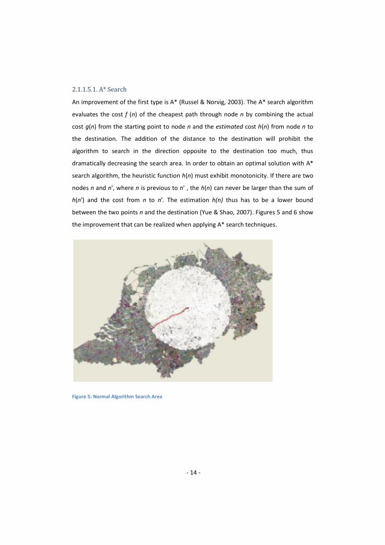
2.1.1.5.1. A* Search An improvement of the first type is A* (Russel & Norvig, 2003). The A* search algorithm

evaluates the cost f (n) of the cheapest path through node n by combining the actual

cost g(n) from the starting point to node n and the estimated cost h(n) from node n to

the destination. The addition of the distance to the destination will prohibit the

algorithm to search in the direction opposite to the destination too much, thus

dramatically decreasing the search area. In order to obtain an optimal solution with A*

search algorithm, the heuristic function h(n) must exhibit monotonicity. If there are two

nodes n and n', where n is previous to n' , the h(n) can never be larger than the sum of

h(n') and the cost from n to n'. The estimation h(n) thus has to be a lower bound

between the two points n and the destination (Yue & Shao, 2007). Figures 5 and 6 show

the improvement that can be realized when applying A* search techniques.

Figure 5: Normal Algorithm Search Area

- 15 -

Figure 6: A* Algorithm Search Area

2.1.1.5.1.1. Haversine Formula

Because every RU is given a unique name based on its location in latitudes and

longitudes, the distance between two points can easily be calculated. The form of the

earth approximates the form of a sphere (Wikipedia, Earth Radius, 2008), therefore

creating the need to calculate great-circle distances (Weisstein, 2008). A good formula

to calculate this great-circle distance is the Haversine formula (Wikipedia,

Haversine_Formula, 2008) because of its ability to calculate accurately on small

distances (Sinnott, 1984)

latitudes and longitudes between two points. A slight deterioration occurs, though,

because the earth is not a perfect sphere. The accuracy can be improved by estimating

earth´s radius for every calculation. For this purpose a formula is used that calculates

the radius of the earth based on latitude. This is done by taking the average latitude

between the two points in the calculation (Wikipedia, Earth Radius, 2008).

2.1.1.5.2. Decomposing the Search Area It is commonly recognized that the computational effort required to solve a problem to

optimality usually grows faster than the size of the problem. As a result, if the original

- 16 -

problem can be decomposed into smaller sub-problems, substantial computational

savings can be realized (Fu, Sun, & Rilett, 2006). Although the distributed nature of the

GATS decomposes the problem into sub-problems already, this will not simply make the

algorithm more efficiently. More calculation time is needed to gather, transfer and

combine the information, while not explicitly cutting the search area.

A method that does cut down the search area is bi-directional search (Fu, Sun, & Rilett,

2006), since it is more efficient to search utilizing both the origin and the destination

uniformly by searching alternatively from the origin side and from the destination side

(Klunder & Post, 2006). Unfortunately this technique is not applicable to the GAT

system. The reason will be discussed in section 2.1.2.1.1. on time-dependent networks.

2.1.1.5.3. Hierarchical Search An improvement of the third type is the hierarchical search method. The hierarchical

search strategy is well known in the artificial intelligence field and is also known as an

abstraction problem solving strategy. The basic idea behind the hierarchical search is

that in order to effectively find a solution to a complex problem, the search procedure

should at first concentrate on the essential features of the problem without considering

the lower level details, and then complete the details later (Fu, Sun, & Rilett, 2006). In

order to make this differentiation the system needs multiple layers of information.

Furthermore, the improvement is very complex and many studies have been dedicated

to the implementation. One issue inherited with a hierarchical search algorithm is that it

usually does not allow any shortcuts such as moving from one arterial road to another

by using a residential road. In a traffic network there usually exist many types of

shortcuts and some of them may even be unavoidable. To overcome these problems,

difficult pre-processing steps will have to be taken (Fu, Sun, & Rilett, 2006) and this

makes this improvement less desirable for non-centralized systems.

2.1.2. Dynamic Shortest Path Approaches

Compared to the static shortest path problem, few works have been done on the

dynamic shortest path problem (Gao, 2005). Two different aspects, i.e. stochastic and

- 17 -

time-dependent networks and the deviation in realization of the route from the plan,

will be discussed here.

2.1.2.1. Stochastic and Time-dependent Networks

There are two ways in which travel times can be changing or even unavailability might

arise. Obviously, not at every point in time there is an equal number of travelers on a

road and accordingly the travel time varies with time. When the number of travelers is

large, this can even lead to recurrent congestion. Recurrent congestion is due to the

mismatch between demand and supply under normal conditions. However, usually

traffic infrastructure is updated in a fairly long cycle. Recurrent congestion is usually

seen in peak hours, but if the capacity is significantly low compared to average demand,

congestion is likely to spread outside peak hours (Gao, 2005).

The other reason for variability in travel times is due to disturbances to the traffic

network. Disturbances, such as incidents, vehicle breakdown, bad weather, work zones,

special events, and so on, occur with various types of predictability. For instance

incidents and vehicle breakdown cannot be predicted and are therefore unavoidable.

Others are predictable to some extent, such as bad weather, work zones and special

events, but usually there are prediction errors. A weather forecast is usually in a

probabilistic format, e.g. a precipitation probability of 90% (Gao & Chabini, 2006).

Completely unpredictable disturbances will be ignored for now, but will be dealt with in

the following part of this chapter on rerouting. The incidences that are to some extent

predictable can be used to create better routes.

2.1.2.1.1. Time-dependent Networks If there is only deviation in travel times due to time, then this can easily be solved.

Although at this time travel times in transportation networks are time-varying quantities

that are at best known a priori with uncertainty (Miller-Hooks & Mahmassani, 2003), in a

totally automated transportation system all future travel times are approximately

deterministic. Figure 7 shows a time-dependent network, where arriving at different

times at node 4 influences the travel time over arc e. The path abe has a length of 10.

This is a lot less then the length of path cde (14), although the difference between ab

- 18 -

and cd is only 1. However, due to the monotonistic character of roads it is never possible

that arriving later at a node will result in arriving earlier at its successor. The information

about incoming cars can be used to predict the travel time over an arc. In order to do

this, the approximate time of arrival of the vehicle at the node is needed, creating the

necessity to search unidirectional. This is the reason that bi-directional search is not an

option for the GAT system.

Figure 7: Time-dependent Network

2.1.2.1.2. Stochastic Networks A stochastic network is a network where the link travel times are random variables with

some a priori distributions. If the underlying network is assumed to be static (non-time-

dependent), the link travel times remain unchanged after they are revealed to the

travelers (Gao, 2005). Figure 8 is an example of such a network. The expected travel

time for path ab is 6+m/2 while for cd this is 7+m/2. It is obvious that it would be best to

travel path ab.

1

2

3

4

a b

c d

(ta, tb, tc, td) = (2,4,3,4)

5e

t = 6: 4 ; t = 7: 7

- 19 -

Figure 8: Stochastic Network

2.1.2.1.3. Stochastic Time-Dependent Networks Of course the travel times can change as well based on both the previous factors. In a

time-dependent network the travel time of every link at every time period is an

individual random variable, so travel times revealed at different time periods could be

different (Gao, 2005). In Figure 9 the travel times are both dependent on the time at

which you cross the arc, but as well on the probability of the occurrence of disturbances.

Here traveling path ab would cost 2,5+7,5=10, while traveling ac would cost 5+6,5=10,5.

Here we would again choose to travel path ab.

- 20 -

Figure 9: Stochastic Time-dependent Network

2.1.2.1.4. Addaptiveness to Time-dependent Information So far, we assumed that the choice of the optimal path had to be made before starting

the trip. However, if the decision which path to take could be postponed until

information about arcs a and c in Figure 8 or arc a in Figure 9 would be available, the

choice would be easier, because now the system would be deterministic in the first case

and only stochastic in the second case. The closer you get to the arc you want to travel,

the more accurate the information will be and the better the choice. The decision rule

which specifies what node to take next out of the current node based on the current

time and online information is called a routing policy. Users are assumed to choose

routing policies rather than paths (Gao, 2005). Although a routing policy will give a

better route, it also requires the system to continuously update information and

recalculate all options and will therefore be much more demanding of the system than a

simple model.

2.1.2.1.5. Equilibrium Assignment Models in Stochastic Time-Dependent Networks Gao (2005) recognizes four different models for networks, the so called equilibrium

assignment models, that distinguish themselves by three features: the knowledge of the

incident probability function, adaptiveness to online information, and optimal adaptive

decision. The policy model is the most advanced and has all the features. It uses

dynamic programming like methods to take the next best step anticipating what lies

- 21 -

ahead. A little less involving is the online path model. It calculates a path with minimum

expected travel time from the current node to the destination based on the current

information and follows the first link along this path. When the user arrives at the next

node, a new minimum expected travel time path is computed and the first link followed,

and so on. This is also an adaptive model. However, it assumes no future change in

network conditions and is therefore a little more short-sighted than the policy model.

The path model is not adaptive anymore. It does consider the random incident, but

users follow simple paths instead of being adaptive. It thus focuses on stochastic

networks. The base model is even simpler. It does not have knowledge of the probability

function of the incident and is model for the simple static situation.

2.1.2.2. Rerouting decisions

Until now, the dynamic models discussed were merely dealing with proactive decision

making. However, when such models are chosen that there exists the possibility of

changing the path along the way, rerouting problems arise. These are reactive models.

There are different models in literature that describe rerouting decisions. The rational-

boundary model (Mahmassani & and Jayakrishnan, 1991), assumes that one reoptimizes

the current route either when the relative difference travel time between two paths is

larger than a predefined relative threshold parameter or when the absolute difference

between these two paths is higher than a pre-defined absolute threshold. In the binary-

logit model (Ben-Akiva & Lerman, 1985) each driver makes its rerouting decision

according to two values; a probability value to change its current following path to

newly found shortest path calculated from binary-logit model and a random value,

representing the modeling error. The probability is based not only on the improvement

of the route, but is representing each

resistance to change the route during the trip too (Yang & Recker, 2006).

Both models, as well as the most involving equilibrium assignment models, assume

knowledge of changes throughout the system. This knowledge makes it possible to

review the current path at every node. Usually, in a distributed system, information is

not shared throughout the entire system, though and since there is no time to

- 22 -

recalculate the entire route at every node, other ways must be found to initiate

rerouting.

2.2. Sorting Problems

The previous section shows that 2 kinds of algorithms can provide solutions to the

shortest path problem; the label-setting algorithms and the label-correcting algorithms.

The first kind produces neatly sorted lists of distance labels. The label-correcting

algorithms do not guaranty these sorted lists after the termination of the algorithm.

Though, for simplicity in back-tracking the optimal path, this is desirable. Several sorting

algorithms are known that can solve this problem. This section discusses some of the

possibilities.

Figure 10: Sorting Methods O(n2)

- 23 -

Figure 11: Sorting Methods O(n log n)

Sorting processes can be very time consuming. The most simple algorithms have a

complexity of O(n2). Figures 10 and 11 show an implementation of some of the different

algorithms. From these figures the huge differences between the various algorithms

become visible. The difference does not only lie within the complexity of the algorithm,

since algorithms with the same complexity can produce very different results.

Dependent on the data series and the problem characteristics, a specific algorithms will

outperform all others. Therefore it is important to assess some of the different

algorithms.

One of the first sorting algorithms to be invented and the most popular O(n2) algorithm

is bubblesort (Astrachan, 2003). Bubblesort is a straightforward and simplistic method of

sorting data, comparing every two items and swapping them if the first is bigger than

the second. While simple, this algorithm is highly inefficient and is rarely used except in

education (Wikipedia, Sorting_Algorithms, 2008).

A better sorting algorithm is insertion sort. This algorithm is often called card sort,

because it works the way most people sort a hand of playing cards. It starts by sorting

the first 2 items. Then it adds the third into its proper place and continues until all items

- 24 -

are sorted. The algorithm is very easy to implement and is amongst the most efficient

when dealing with small or nearly sorted lists. Still, the average and the worst-case

complexity are O(n2).

Both sorting algorithms described above work by comparing different items to each

other and are therefore called comparison sort algorithms. In theory, these algorithms

have a lower bound complexity of O(n log n). An example of an algorithm with average

complexity of O(n log n) is quicksort.

Quicksort works by partitioning all the items around a pivot and recursively sort the sub

lists of items larger and smaller than the pivot (Wikipedia, Quicksort, 2008). Ideally,

quicksort partitions sequences of size N into sequences of size approximately N/2, those

sequences in sequences of size N/4, and so on, implicitly producing a tree of sub

problems whose depth is approximately log2 N. Sequences that cause many unequal

partitions result in the growth of the sub problem tree in a linear rather than a

logarithmical way. This is for instance the case in partially sorted lists (Musser, 1997).

Another problem encountered in quicksort is that it does not work very efficiently for

small sub problems (Sedgewick, 1987). It is very strong, though, for large lists of

randomly sorted items and in practice it is in fact faster than most other sorting

algorithms (Musser, 1997). This makes quicksort one of the most popular sorting

algorithms, available in many standard libraries (Wikipedia, Sorting_Algorithms, 2008).

The literature provides some solutions to solve the weaknesses of quicksort. To avoid a

linear growth of the problem tree, Sedgewick (1987) suggests that a median of 3 items

be used as a pivoting item. However, sequences can be found that will still have a

complexity of O(n2) under the median of 3 strategy. Rather than a median-of-3 items

Musser (Musser, 1997) proposes a limit on the depth of the search, to limit the

complexity to O(n log n), although recognizing the fact that the probability that these

sequences occur is very small.

The inefficiency and storage space requirements can be solved by choosing a different

method for small sequences. Leaving small sub problems to insertion sort is one of the

- 25 -

usual optimizations of quicksort (Musser, 1997). Because the number of recursive

calculations will increase exponentially with the number of divisions, aborting the

recursive process for small sequences will save a lot of memory. The result thus will be a

hybrid method capable of choosing the most efficient sorting scheme based on the

length of the sequence.

- 26 -

3. Algorithm Formulation

The algorithm for the GAT system is described in this chapter. The basis for the creation

of this algorithm is the shortest path algorithm. An overview of the literature suggests

that, given the specific distributed architecture of the GAT system and given that the

algorithm will deal with real road networks, the Pallottino algorithm is the best choice.

This algorithm gives the possibility to use multiple starting points at the same time and

easily combines information from multiple calculations. However, the algorithm does

not produce entirely sorted lists. Given that the results of the algorithm will already be

partially sorted, the choice of the insertion sort algorithm is logical for small lists. For

longer lists the quicksort is better suited.

The Pallottino algorithm, combined with the 2 sorting algorithms will be the main part of

the algorithm. We guide the creation of the rest of the algorithm by the use of an

engineering framework. The logical steps of the framework can be put almost one-on-

one with the sections of this chapter.

3.1. A Multi-Agent Engineering Framework

The framework of Wood & DeLoach (2000) (Appendix A. MaSE Framework)is particularly

useful because it takes an initial system specification, and produces a set of formal

design documents in a graphically based style. The graphical, universally accepted style

makes sure that both the steps in the process of creation and the algorithm itself are

understandable for others. Moreover, since the methodology is independent of

particular multi-agent system architecture, agent architecture, programming language,

or message-passing system, it will not influence the implementation of our results. The

framework is a little bit too extended though for this purpose, so we will not follow

every step as extensively and focused mainly on the analysis part of the framework.

We follow the steps of the framework in order to answer the following questions:

a. What are the requirements of the system?

b. What are the goals of the system?

c. What do the processes of the algorithm look like?

- 27 -

d. What information passes through the system?

e. What actors can be identified in the system?

f. What are the tasks and procedures that these actors have to perform?

3.2. Transportation System Requirements

The first step of the framework determines the system requirements. As explained, we

focus on a static system with just one car. This means that the requirements at this time

are different from the ultimate system requirements. In this phase the system should be

able to:

1. Calculate a shortest path from source to destination.

2. Limit the search area by excluding regions that are unlikely to contain the

shortest path.

3. Use any number of region levels without changing the algorithm (scalability).

4. Store the future arrival of a vehicle in a RU when this RU is on the shortest path

in combination with the arrival time.

5. Exclude particular roads for particular vehicles, either because of temporary

unavailability or because of structural inaccessibility to that kind of vehicle.

6. Calculate the shortest path based on real time information.

7. Calculate the shortest path based on time or absolute distance.

8. Adjust the travel time based on car characteristics.

9. Sorting out useful information and deleting useless information from system

memory.

3.3. Transportation System Goals

In the next step we transform the initial requirements into a structured set of goals. This

means both identifying and structuring the goals. The result of this structuring process is

- 28 -

a hierarchical goal-tree where all sub-goals relate functionally to their parent (Wood &

DeLoach, 2000). One of the requirements of the system is that it is perfectly scalable.

For this purpose we add a recursive element to the system. This recursive element is not

easily made visible in a tree structure. So for clarity we sketch a situation with just 1

level.

Appendix B presents the goal-tree. This figure visualizes that the goal of creating a

shortest path is supported by the goals of choosing the search area, sending and

receiving information of the down lying regions, storing this information and using it to

create the shortest path. In the recursive algorithm, all these goals will be full-filled

multiple times.

3.4. A Detailed Transportation System Description

The third step of the framework consists of the creation of use cases. Use cases are

descriptions of system behaviour as it responds to a request that originates from outside

of that system (Wikipedia, Use_Case, 2008). They describe in a narrative way what we

want the system to do in what situation. One of the benefits of use cases is that they put

requirements in context, describing them in a clear relationship to tasks. For now, we do

not make a clear distinction between the different use cases. Rather we will provide a

detailed system description, explaining all actions and functions. In this description we

sometimes make some side trips, that, strictly speaking, might not be part of the use

cases, but that do give a broader understanding of the systems working.

Consider a vehicle at a random starting point A that wants to travel to destination B.

After entering this destination the vehicle seeks contact with the nearest RU. This

request contains the request for an itinerary to the destination, but also characteristics

about the vehicle, the kind of vehicle and whether you want to follow the shortest route

or the fastest route. We will call this information (reflected in Appendix D)

every level controller during the process of creating the shortest path.

- 29 -

The vehicle characteristics are important when calculating the fastest route because the

engine power, acceleration speed, maximum speed and vehicle weight, among others,

will influence the travel time. Of course, these characteristics do not have the same

effect on every road. On a highway the maximum speed matters more than the

acceleration speed. In this phase of the project we keep the information pretty basic

though, but it can easily be made more realistic later. The kind of vehicle is important

because not every road is accessible to every kind of vehicle. Trucks are often banned

from city centres or mountain passes, while small motorized vehicles might not be

allowed on highways. If the road is temporarily unavailable due to weather conditions or

other circumstances, the accessibility can be turned off for every type of vehicle.

A RU does not calculate shortest paths. This is done by the controllers, so the RU will

immediately pass this message on to the level 1 controller. The controller picks the

starting point (A) and starts calculating the shortest path using Pallottino´s algorithm. At

this point, every arc is evaluated on accessibility and current travel time based on both

vehicle and road characteristics. This evaluation is done by the RU, because this agent

has knowledge of the status in real-time, so the controller will receive a travel time and

a travel distance.

+LocationOfOrigin = 0+LocationOfDestination = 1+TravelTime/DistanceToDestination = 2+LvLControllerOfInvestigation = 3+LvlControllerOfOrigin = 4+Optional: TravelTimeToDestination = 5

«enumeration»GeneralInformationStorageFile

Figure 12: General Information Storage File

For every point (1, in Figure 12) and vehicle not only the travel time is stored, but also

the previous point visited (0) to get to that point and, if the RU is a border point

between two regions, the name of the region that is not being investigated now (3). This

last information has two purposes. First we immediately know what RUs are border

points and second we know what the next region is that we want to explore without

- 30 -

consulting the particular RU. The region we are exploring now is also stored (4) because

we need this information when we want to back-trace our path after finding the

destination. Both travel time and distance can be passed because, when calculating the

shortest distance path, the time of arrival needs to be stored and thus known in the end.

Therefore a place is reserved for travel time (5) in case (2) is travel distance. All

information about the passing RUs is thus stored in arrays of the type

Information Storage Files:

If all points are evaluated and the destination is not reached yet, then a selection of

nodes has to be made. All the information about nodes that are on the border of two

regions will be send to the appropriate higher level controller. This information is always

accompanied by the information about the vehicle. Here, the information about the

border points (3) is needed, because we can easily separate the border from the non-

border points.

The level 2 controller now has information about the travel times to all the borders. It

will ask all the regions that have RUs on the border of the already calculated area to

start calculating from these known points. The information about the arrival time of the

car is passed. The RU requires this information to give a good estimation about the

travel time at the moment in time at which the car arrives. Once the RU is selected as

the next RU to explore, the LvLControllerOfInvestigation information is altered to

indicate that the points are already investigated and thus to prevent calculating from

the same points over and over again. When all regions have been calculated and the

destination is not found, again the information will be send upwards.

Unlike in the lower levels, where the computational time needed to explore all RUs is

still limited, the search in the higher level controllers will continue one region at a time.

The next region to be explored will be based on a heuristic approximation of the total

distance or time to the destination. So the way the A* method chooses the next node, in

the GAT the next region will be selected. Because while it might be profitable on lower

levels to drive away from the destination, for instance to prevent crossing a large and

- 31 -

busy city centre, on higher levels, province or country sized, the direct approach is most

often the best.

The process described above will continue until the highest necessary level (the level m

controller) that involves both the starting point and destination. As explained above,

before sending the information to higher level controllers a sorting procedure is

executed.

Although the GATS is a driverless system, this does not mean that there is no human

agent inside the vehicle. So we still identify the driver, as the person that wants to drive

from starting point to destination. This driver is an important part of the system and

influences the requirements. A driver would for instance feel very uneasy driving

towards another vehicle, without a clue if his vehicle would slow down (Labiale, 1997).

So there is a need to let the driver know what is going to happen. That also means that

although normally all information is stored distributed over all level controllers, there

has to be a central knowledge of the route as well, at least in the vehicle. Therefore,

after creating the shortest path, the entire path will be transferred to the starting RU,

which will communicate it back to the vehicle.

Both to visualize this information and to be able to enter a destination into the system,

the vehicle should be aware of the entire static system, i.e. the location of the RUs and

the present arcs between these RUs. For this reason a system is needed that allows us to

quickly find the locations. Since the internet is a distributed system as well with a system

that has already proven itself, we propose a similar system for the level controllers in

GATS. The Internet uses the so called Domain Name System (DNS) (Wikipedia,

Domain_name_system, 2008). In DNS, different domains exist at different levels. Every

might be the top level domain, having a sub doma

contain the names of all its parents.

- 32 -

Although this system makes it very easy to see what is the first level controller shared by

both starting point and destination, this is not necessarily the level m controller. Only in

the case of convex regions can this be guaranteed. A region is said to be convex if every

point on the line segment between two points (x,y) in this region lies within the region

(Wikipedia, Convex_set, 2008). In case of non-convex regions the optimal path might

lead through a different level controller of the same level and thus need a higher level m

controller. Of course a lower level m controller is never possible. The example of Figure

13 shows a planned route (Google, 2008) between 2 points in Spain leading through

Portugal and thus needing a higher level controller than the one controlling only Spain.

Even though a region might look geographically convex, the fact that most often travel

times are used for the determination of the used path can make the region lose its

convexity.

Figure 13: Concave region

The level m controller will calculate the shortest path between the points A and B. After

finding the shortest path, all RUs need to be informed of the path that will be taken.

Therefore the controllers will pass this message on down until it reaches the RUs, at the

same time, the information about the entire path will be sent up, so that it can be sent

to the car. Furthermore all stored information about the vehicles possible routes will be

deleted from the memory.

- 33 -

3.5. Information Flows in the Transportation System

The narrative description of the system is visualized in this phase into the sequence

diagrams of Appendix C. These make the information flows visible among the different

agents. Any communication between different levels is visible here in the form of an arc

between the two regions. From Figure 21 it becomes clear that the calculations start in a

small region around the starting point and spread in the direction of the destination

with the increase of the number of the level of the controllers. As well it can be seen

that the request for information at the level 1 controller triggers the execution of the

Pallottino algorithm

return arcs. lised once, but are of course executed

every time. The procedures are thoroughly explained in chapter 3.7.

Figure 22 shows the process of informing the RUs of the arrival of a vehicle after the

shortest path has been found. After this information has passed through the system, the

path will be sent to the vehicle and all stored information will be deleted. This last

process has a sequence diagram very similar to that of informing the RUs of the arrival

of the vehicle. The main differences are that it´s only a downwards process and it affects

all down lying level controllers instead of only the ones on the shortest path. Because of

these only minor differences the process isn´t shown in a separate diagram.

3.6. Actors in the Transportation System

Both in the system description and in the sequence diagrams from the section above, a

lot of actors are already introduced. This section gives a full explanation of all actors,

though, and more importantly, it gives an overview of the different roles that the agents

can take.

Although there are only few agents that seem to interact in this system, we can define

multiple different roles within these seemingly simple agents. The simplest role is that of

the RU. This role is responsible for the realization of the goals that have to do with the

time or distance measurement and are defined by area A (Appendix B). Normally goals

and roles exist one-to-one, however similar or related goals might be combined into one

- 34 -

role (Wood & DeLoach, 2000). The RU interacts with the car and the level 1 controller,

which we will both define as roles too. Although the car can be used as an agent, in the

algorithmic part of the research it hardly plays an important part and is mainly used as

an initiator for the processes.

Not every level of controllers needs to be identified as a different role, since most

controllers react in the same way. Of course this is inherent to the requirement that the

system should be extendable to as many levels as required. The controllers realize all

the goals in area B of Appendix B. However there are some differences. The lower level

controllers determine the shortest paths by requesting the information about all

possible points (current borders of the investigated area) at the same time, while the

higher level controllers only calculate the most promising region. The controllers all have

to receive and send information to higher and lower level controllers or RUs, except for

the level m controller, which only communicates with lower level controllers. Most level

controllers coordinate with other level controllers, while the level 1 controller also

coordinates with RUs. Depending on the route and preferences, a level controller could

take any of these roles or multiple at the same time. Therefore we define the above four

controller roles, but have them all carried out by the same agent.

When we look at our class structure (Appendix D), obviously we define the different

agents as classes, but we also add another: the arcs. These contain the static

information about the road network in the system.

3.7. Specific Algorithm Tasks and Procedures

At this point the general way of working of the algorithm is clear, as are the agents

participating in the system and the system goals. Therefore we can now specify the

specific tasks and procedures of which the algorithm is made up. With the tasks and

procedure diagrams presented in this section, the code behind the tool of chapter 4. and

our algorithm becomes clear. The other way around, we use the tool to clarify the

procedures and tasks.

- 35 -

The different tasks that have to be performed are visualized in task diagrams (Appendix

E). In the diagrams, the nodes represent the processes, while the arcs represent

information flows, information changes or decisions. The tasks are carried out by one

single role and thus by one agent. However, multiple tasks can be performed

waiting

started and that the return of that task is input for the continuation of the task.

Within the tasks, there are subtle differences between the situations where the tasks

are requested by a higher level controller (Figure 26, Figure 28 and Figure 30) or by a

lower level controller or RU (Figure 25, Figure 27 and Figure 29). The search area is

always expanded by a request to a higher level controller. After that the search is

continued to the lower level controllers that return the information. Therefore, the fact

that a task of a level controller is requested by a lower level controller means that the

executing level controller is the highest level controller at that time and thus possibly

the level m controller. If it is the level m controller the task will end and no other task

will be executed, otherwise the task will end by expanding the search area even more. It

holds as well that a level controller task that is requested by a higher level controller can

neither contain the creation of the ultimate shortest path nor the informing of the RUs

of that path. Therefore these tasks always end by returning the border-to-border

information to the higher level controllers. Another difference between the two

situations is that in case of a request of a lower level controller, there a no starting

points yet, while a request from a higher level controller is always accompanied by a set

of starting points.

Also it can be noticed that the task will continue until either no more border points of

the search area can be found that are within this level controllers region or the

destination is found. This last event will only initiate a new procedure (inform RU of

arriving vehicle) if the task is requested by a lower level controller. The procedures of

informing the RU of the arriving vehicle and deleting the information are not

represented in task graphs. Although these procedures will trigger tasks at the different

- 36 -

level controllers, these tasks are very simple and will be only displayed in the form of a

procedure.

process indicates the initiation of another task and tasks can

serve as input for other tasks. Therefore we indicate the relationships between the

different tasks. In Figure 23 the request for the shortest path (indicated by

newDestination ) is passed to a level 1 controller. This is the initialization of the task in

Figure 25. In Figure 25 and Figure 26 waiting

Figure 24. For Figure 27 to Figure 30 it is not directly certain which task is initiated since

it is dependent on the level of the level controller and the place of the border between

lower and higher level controllers.

Next we will provide some explanation to the diagrams that describe the different

processes or procedures of the algorithm. The procedures go from start to finish and use

the input from the parallelogram directly following the start node. The squares are other

procedures that are called, while the rounded rectangles represent actions in the

procedure itself. The diamonds are conditional nodes, where the options are on the arcs

leaving the node.

- 37 -

If Destination =Found

Calculate Downwards (without StartingPoints)

start

-Car

Case LvLController.LvL=1

Set the StartPoint as the CarsCurrent Location

1<Lvl<=CalculateAllLvL

Finish

CalculateDownwards(StartPoint,

DestinationFound)

To LvlUpController:Calculate

Downwards(without

StartPoints)

Sort and Store thegathered

information: (A)


InformRUsOfArrivalVehicleTrue

Sort and Store theGathered

information: (A)

LvL>CalculateAllLvL

True

Finish

At least 1 Item of (A) withLvlControllerOfInvestigation =

LvlController

False

Divide All Rus for Investigation among itsLvlDControllers

True

For AllLvLDControllers:

CalculateDownWards(StartPoint)

ReturnTheMostPromosingRU

False

LvLControllerMostPromosingRU =

LvLController

Find All Rus that belong to sameLvLController at CalculateAllLvL

True

For 1LvLDController:


Find the correspondingLvLDController

FindBorders of theSearch AreaFalse False

Save at Higher LvlController

Finish

ForLvlUpController:

CalculateDownWards(withoutStartPoints)

DeleteInformation


False

True

Update SavedInformation to indicate thatStartingPoints are used


calculate downwards without starting points. This

procedure is the beginning of the main iterative procedure and is always called by the

highest level controller involved in the calculations at that moment. The procedure will

be different for the different roles of the level controller and we will separate three

separate possibilities; level 1, below the level where we calculate everything and above

this level. The last two possibilities might never occur, depending on the height of the

level below which we calculate everything and the distance between the starting point

and destination.

- 38 -

If the level is level 1, then we set the current location of the vehicle as the starting point

and we call the next procedure . After the

procedure returns and the destination wasn´t in the same region, the search area will be

expanded by making the level 2 controller the highest level controller. Otherwise the

RUs will be informed of the arrival of the car and the car will be informed of the journey.

If the controller is of a higher level, then the procedure starts by finding the initial

- , these are all the unexplored points

- , this is the set of points

belonging to the region of the most promising RU. However, it is possible that multiple

calculations after each other are executed in the same region. Therefore, after the first

calculations based on the initial found starting points have finished, a check is added to

see whether the next RU that has to be explored belongs to this area. If this is no longer

the case, then again the search area is expanded.

Every time calculations are carried out on level controllers higher than level 1, the saved

information will have to be updated to indicate that the border points are used as

starting points. Otherwise, the procedure will be appointing the same border points all

the time as starting points and will get stuck in a loop.

Because this procedure is always executed by the highest level controller in the search

area, this controller also has the possibility to calculate the ultimate shortest path after

the destination has been found.

- 39 -

Calculate Downwards (with Destination Check)start

-Car-StartPoint:

GeneralInformationStorageFile

-DestinationFound:Boolean

Finish

CalculateShortestPath With

PallottoniAlgorithm

FindBorders

StoreUpWithoutOverwriting


FalseTrue

Result:=DestinationFound

is the next procedure. This

-procedures only for the

level 1 controller. After calculating the shortest paths through the level 1 region, this

procedure decides either to store the starting point to border information at the level 2

controller or to return a message that the destination has been found.

- 40 -

Calculate Downwards (StartingPoints)start

-Car-StartPoint:


Case LvLController.LvL=1

1<Lvl<=CalculateAllLvL

Finish

CalculateShortestPath With

PallottoniAlgorithm

LvL>CalculateAllLvL

At least 1 Item of (A) withLvlControllerOfInvestigation =

LvlController

Divide All Rus for Investigation among itsLvlDControllers

True

For AllLvLDControllers:


ReturnTheMostPromosingRU

LvLControllerMostPromosingRU =

LvLController

Find All Rus that belong to sameLvLController at CalculateAllLvL

True

QuickSort

StoreInformationHigherLvLController

Finish

For 1LvLDController:


False

False

FindBorders

StoreInformationHigherLvLController


Reload gatheredInformation

FindBorders

Reload gatheredInformation


If Destination<> Found

True

False

is very similar to the other

two. It does not have a destination check at the first level, because it is already known

that level 1 is not the highest level if this procedure is called at all. For the higher levels

there are three main differences. First, there is no need to do the initial calculations,

because the starting points are already provided. Second, since this is never the highest

level controller, no ultimate shortest path will be calculated and last, after the discovery

of the destination, the current calculations are finished, but no new ones are started.

The real calculation of the shortest path in the level 1 Pallottino

algorithm . This algorithm is a label updating algorithm and uses 2 queues and 2 lists.

- 41 -

First these lists and queues are loaded. The starting points go to the priority queue (Q1),

the other RUs go to the list of unvisited items. The distance to these RUs is infinite if this

is the first time the region is explored or equal to the found minimum distance in the

previous exploration. The other list contains the already checked RUs. When RUs are

moved from the queues to the visited items list, the distance to the RU combined with

the distance to its successors is compared to the existing distance label of the

successors. If the distance is shorter, the label is updated and the RU is moved into a

queue, if it is not yet in one. If the RU was in the visited list, it will be added to the

priority queue, RUs from the unvisited items list enter Q2. After the procedure is

finished, the list is sorted and saved.

- 42 -

Pallottoni Algorithm

start

-StartLocation,-Rus:


Add Rus to UnvisitedList (U)

Add StartLocations to Q1and delete from U

If Q1<> empty If Q2 <> emptyFalse

Move RU from Q1 toVisited List (V)

True

Add the information aboutLvL Up Controller

Return Arcs

If distance tosuccessor <

currently stored

Move successor from (U) to Q2 orfrom (V) to Q1, or update if already in

Q1,Q2.

True

Move RU from Q2to (V)

True

Quicksort

False

Save withOverwriting

Finish

False

Check ifDestination

AddLvLControllerOfOrigin True

Result:=DestinationFound

that finds all links and travel distances and converts these into a travel time based on

the maximum speed on the arc at that particular time, the maximum speed allowable

for that type of vehicle in that region and the maximum speed of the car. It eliminates

arcs that are unavailable to the vehicle, either because of congestion or because of

structural unavailability to this type of vehicle.

- 43 -

Return Arcsstart

-Car

If # Arcs > 1

True

Check for All Arcs ifAvailable for Car

If RequestType =Shortest Path

True

True

Add Arc to Result

FalseFind the minimum of thecountrys, the cars, or thecurrent roads max speed,

Convert thedistance to time

Finish

procedure sorts the RUs on distance or travel time. The method is calling

itself recursively for smaller sub lists. Therefore the minimum and maximum number of

the list are added to indicate the position and size of the sub list. If the length is smaller

than 9, the list is sorted by the procedure. If not, the method finds the

median of the first, middle and last RU of the list. The items are moved around this

number, the higher numbers on the right, the lower on the left.

- 44 -

Quicksortstart

-Rus:GeneralInformationSto

rageFile-Min,Max: integer

Finish

If max-min <= 7True

False

InsertionSort(Rus,min,max)

Find median of min,max, 0,5*(min+max)

Divide the Rusaround the Median

QuickSort ListLower than

Median

QuickSort ListHigher than

Median

- 45 -

Insertionsort

start

-Rus:GeneralInformationSto

rageFile-Min,Max: integer

Finish For (i) = min + 1 tomax and (k) = (i)-1:

Copy RU (i)

While distanceto Ru (k) < (i)

Move RU (k) up

True

Decrease (k)

False

Copy RU (i) to (k)

is

used, because after the ´Pallottino all the RUs are in the list and have the

lowest possible value.

Save with Overwriting

start

Rus:GeneralInformation

StorageFile-Car

Finish

File (F1):LicencePlate.ControllerName.

Visited.txt Write Rus toTextFile

Not all information will be sent to the higher level controllers. Therefore the procedure

selects the proper information. There are two cases that can be separated;

- 46 -

either the destination is found already, or it is not. If the destination is found, only the

distance to the destination is valuable information. So this is saved and the ultimate

predecessor in this region is back tracked. Otherwise, all RUs that haven´t been

investigated yet are selected and combined with their ultimate predecessors.

Find Bordersstart

-Arcs:GeneralInformationStorageFile


For All Arcs if =Destination

True

True

If Region Border Node

True

Add to Result With RegionBorderNode as LocationOfOrigin

FalseFind the predecessor of this

RU

For All Arcs iflvlControllerOfInvestigation =

Unvisited

True

If Region Border Node

True

Add to Result With RegionBorderNode as LocationOfOrigin

False

Finish

Find the predecessor of thisRU

False

Multiple level down controllers have to save their information at the level up controller.

If they would save their information and overwrite old information, most information

would get lost. Moreover, because a region might be explored multiple times from

different starting points, information might be passed up multiple times. Therefore the

procedure will check whether the RUs are already in the list

and adds or updates the RUs.

- 47 -

Save without Overwriting

start

Rus:GeneralInformation

StorageFile-Car

Load the info from Text File

If TextFile already exists

TrueTrue

For all Rus: compare with info andUpdate info

Finish


Visited.txt

False

Write the Rus toTextFile

finds the location of all the unexplored

points and the destination in terms of latitude and longitude. Then the procedure

e uses the haversine formula to calculate the distance

between the two points to find the

most promising region based on the total expected distance.

- 48 -

ReturnMostPromosing RUstart

-BorderPoints:GeneralInformationStorageFile

-Car: Car

Finish

True

Return:= BorderPoint

For all BorderPoints:Calculate Latitude and

Longitude of BorderPoint

Calculate Latitude andLongitude of Destination

Calculate Distanceon a Sphere

If TravelDistance+ Distance on Spherical Earth

= Smallest so far

If RequestType =ShortestPath

False Divide Distance byMaxSpeed

True

- 49 -

Calculate Distance on a Sphere

start

-BorderPoint:Lat,Long

-Destination:Lat,Long

Finish

Calculate the Distance withHaversine Formula

Calculate Latitude andLongitude of BorderPoint

Calculate the Approximate EarthRadius based on Average Latitudes

Convert the positions to radials

is a recursive formula that starts at the

destination at the level m controller and back tracks the route over every level. It stops

at the starting point of a region, because that is the end point for another. The level

m controller is

aware of the entire path and can send it to the vehicle. After that there is no more use

for the stored information and the procedure will, surprisingly,

delete all information stored by the level controllers.

- 50 -

Inform RUs of Arrival Carstart

-Car: Car-EndPoint:Extended

Finish

False

ArrivingCarList

True

Load Saved BorderInformation

If Lvl = 1

True

Whilepredecessor =

found

Whilepredecessor =

found

False

InformRUsArrivalCar(Car,

Predecessor)

True


Visited.txt

Find LvlDControllerCorresponding to

LvlControllerOfOrigin ofPredecessor

Add to Result

Add to Result

Delete Information

start

-Car

If LvL=1

True

Finish

False

Delete (F2)

For all LvlDownControllers:

DeleteCarInformation


Visited.txt

Delete (F2)

If File existed

True

False

- 51 -

4. Evaluation of the Algorithm and Tool-design

To test the algorithm we have developed a tool, using Borland Delphi. This tool uses a

simple test case based on a small part of Valencia. The first part of this chapter discusses

the features of this test case to get some basic knowledge of the tools working. Then we

explain the working of the algorithm with the help of an example. In the third part of

algorithm. With this comparison we can evaluate our algorithm and make some

conclusions about the quality of our algorithm.

4.1. Tool for the GAT system

In this part we explain what the major features of the tool and the test case data are.

The test case is based on real locations, because the algorithm uses latitudes and

longitudes of locations. Therefore we picked an area of points abcd (Figure 14). These

points mark the boundaries of the highest level controller (a level 3 controller). The

highest level controller has four lower level controllers (the controlling area of the first

level 2 controller is marked in the left upper corner) and all of these level controllers

again have four lower level controllers. This creates the 16 regions in Figure 14. In the

tool we represent the regions by numbers counting from left to right, from top to

bottom. Since we use an internet-like naming system, the regions inherit the names of

their parents. So the region in the top left corner is called 111, where the first 1 stands

for the top left position of the level 1 controllers, the second for the top left position of

the level 2 controllers and the third because there is just 1 level 3 controller. This means

that the name of the bottom right region is called 441. In every region 5 points are

randomly picked, creating 80 RUs. However, due to the fact that every border point

belongs to two different regions, the number of RUs in the regions will be larger than 5.

The small size of the test case creates a ratio of border-to-non-border-points that is

much higher than in real situations. Therefore RUs are likely to connect more than 2

regions, which is impossible for this algorithm. To solve this problem we created virtual

RUs close to the RUs that had this problem. These virtual RUs will be used to create

paths, but can never be a starting point or destination. The lengths of the arcs are

- 52 -

calculated based on a small factor combined with the lower bound distance between

the two real points, while the travel speed is set equal to 45 for simplicity.

Figure 14: Map Area in Tool

The tool allows us to select different options based on the requirements of the GAT

system specified in chapter 3. These requirements can be separated into two categories,

routing characteristics and car characteristics. Under routing characteristics one can

choose the CalcAllLevel. This is the level up to which one considers all down lying points.

Above this level, the algorithm will switch to a choice of the next region based on the A*

method. There are three possibilities: even the level 1 controllers will be chosen by the

A* like method, only the level 2 controllers will be chosen based on this method or none

of the controllers will be chosen this way. Furthermore the current location and the

destination can be chosen. After entering the locations, the tool will show the two

points and a route between the points based on the Google maps functionality. This

route doesn´t represent the route chosen by the algorithm because the test case

doesn´t follow the real roads, but it allows us to get some feeling about the route. Last,

there is a possibility to choose either a fastest routing approach, based on time, or a

shortest routing approach, based on distance.

- 53 -

The car characteristics contain the vehicle type, the speed and the acceleration. This is

not a very exhaustive representation of a vehicle and definitely not realistic, but it

requires the system to account for differences between vehicles and this makes the

system easily adaptable to different inputs. After entering the car characteristics, the

tool can be initialized, which enters the current preferences into the system and the

search can be started. The information that would normally pass back to the vehicle

now will be shown in the tool; the name of the passing nodes and the time of arrival at

these nodes.

Figure 15: Tool Interface

4.2. Example of the Algorithm in the Developed Tool

In this part we follow the algorithm in its calculations of the shortest path between two

randomly chosen points of the test case. More than the theoretical description in the

previous chapter, this will give insight into the workings of the algorithm. We show at

what times the different procedures start working and why certain choices are made. To

be able to explain this properly, we present the inputs and outputs to different

- 54 -

procedures in table format. From the enormous amounts of information we indicate

what is important and notable.

We initiate the system. Let´s assume we´re at starting point A, with coordinates

(39.465572, -0.344496), which lies in region 431. We want to travel to destination B at

location (39.473347, -0.339594). The CalcAllLevel is set at 2.

Figure 16: Starting Point Example

- 55 -

Figure 17: Destination Example

pallottino algorithm . In the

initialization of this procedure all RUs from the level controller will be divided amongst

the lists. The starting point(s) will go to Q1. In this case only one RU will go to that list

(Table 1), our current location A. The rest of the RUs are added to the list of unvisited

RUs. 7 RUs are now in this list, the distance to each of these is marked as infinite.

From: To: Distance (in minutes):

Region of Investigation:

Region of

Origin: (39.465572, -0.344496) (39.465572, -0.344496) 0.0000 -1 - Table 1: Starting Point 431

The algorithm picks the first starting point from Q1, moves it to the visited RU list and checks if this is a border point of the region. In this case, the starting node is not a border point, so we do not have to add any region information. Therefore we immediately start looking for the arcs emanating from this point by calling the

. We only select the ones that lie within this region. We find that there are four RUs we can add to Q2. We update the distance to these points and now have the following queue:

From: To: Distance (in Region of Region

- 56 -

minutes): Investigation: of Origin:

(39.465572, -0.344496) (39.465205, -0.347125) 0.3149 - - (39.465572, -0.344496) (39.465397, -0.346526) 0.2408 - - (39.465572, -0.344496) (39.465907, -0.344935) 0.0728 - - (39.465572, -0.344496) (39.467125, -0.343259) 0.2783 - - Table 2: Q2

The Q1 is empty, so we have to pick from Q2 now. We pick the first RU from the queue

and check if it is a border point, which again it is not. Therefore we move it to the visited

list and proceed to find all the emanating arcs:



Region of

Origin: (39.465205, -0.347125) (39.465655, -0.349067) 0.2390 - - (39.465205, -0.347125) (39.466674, -0.347921) 0.2431 - - (39.465205, -0.347125) (39.465572, -0.344496) 0.3149 - - (39.465205, -0.347125) (39.465397, -0.346526) 0.0764 - - (39.465205, -0.347125) (39.465907, -0.344935) 0.2795 Table 3: Arcs from RU

Note that the third arc is going back to the origin and that the last two arcs are pointing

to points that are already in Q2. We add the first two RUs to Q2 and compare the last

three on the total distance. Obviously this will lead to the omitting of the path to the

origin, but the other paths are less desirable than the already known labels as well. For

instance, the distance to (39.465397, -0.346526) through (39.465205, -0.347125) will

take 0.3149+0.0764=0.3913, which is larger than the already known distance of 0.2408.

So this will give a new queue Q2, with updated distances and locations of origin:



Region of

Origin: (39.465572, -0.344496) (39.465397, -0.346526) 0.2408 - - (39.465572, -0.344496) (39.465907, -0.344935) 0.0728 - - (39.465572, -0.344496) (39.467125, -0.343259) 0.2783 - - (39.465205, -0.347125) (39.465655, -0.349067) 0.5539 - - (39.465205, -0.347125) (39.466674, -0.347921) 0.5580 - - Table 4: Q2

This process will continue until all RUs in the region have the lowest possible label. Then

the information will be stored by the procedure The final

information will be stored like this:

- 57 -



Region of

Origin: (39.465572, -0.344496) (39.465572, -0.344496) 0.0000 -1 - (39.465572, -0.344496) (39.465907, -0.344935) 0.0728 231 431 (39.465572, -0.344496) (39.465397, -0.346526) 0.2408 - - (39.465572, -0.344496) (39.467125, -0.343259) 0.2783 231 431 (39.465572, -0.344496) (39.465205, -0.347125) 0.3149 - - (39.465397, -0.346526) (39.466674, -0.347921) 0.4958 331 431 (39.465397, -0.346526) (39.465655, -0.349067) 0.5428 331 431 (39.467125, -0.343259) (39.468527, -0.341495) 0.5768 141 431 Table 5: Saved Information Level 1 Controller 431

We can see that there was only one starting point in this region (indicated by -1), that

there are 2 RUs that have no connection to other regions (indicated by the blanks in the

region fields), four RU´s that have a connection to a region that has the same level 2

controller (31) and one with a connection to a region that only has the same level 3

controller (1). The procedure will filter out all the useful information for

the level 2 controller and replace the current origins of the arcs with the ultimate

predecessors. In this case, all paths originally start at the starting point A. Therefore the

following information will be stored at level 2:



Region of

Origin: (39.465572, -0.344496) (39.465572, -0.344496) 0.0000 -1 - (39.465572, -0.344496) (39.465907, -0.344935) 0.0728 231 431 (39.465572, -0.344496) (39.467125, -0.343259) 0.2783 231 431 (39.465572, -0.344496) (39.466674, -0.347921) 0.4958 331 431 (39.465572, -0.344496) (39.465655, -0.349067) 0.5428 331 431 (39.465572, -0.344496) (39.468527, -0.341495) 0.5768 141 431 Table 6: Saved Information Level 2 Controller 31

The search area is expanded and the level 2 controller (31) is now the highest level

controller. Because the level below which we calculate everything is level 2 we select all

the border points of this region for the new search. This means we get two sets of

starting points. These two sets will normally be calculated at the same time by two

different level controllers. However, in our tool they have to be calculated consecutively.

- 58 -



Region of

Origin: (39.465907, -0.344935) (39.465907, -0.344935) 0.0728 -1 431 (39.467125, -0.343259) (39.467125, -0.343259) 0.2783 -1 431 Table 7: Starting Points 231



Region of


will be executed for both

regions. When the regions 231 and 331 will execute the , we will

know a distance to all the reachable RUs in those regions. Here it becomes clear why it is

useful to have a label-correcting algorithm. Labels to RUs in the regions will differ based

on which of the 2 RUs we take as starting point. It might even be faster to go through

one starting point to the other. The label-correcting algorithm can update the labels

every time a better solution is found and therefore we only have to do the calculations

once, instead of once for every starting point. The results are saved and the border to

border information is sent up to the level 2 controller:



Region of

Origin: (39.465572, -0.344496) (39.465572, -0.344496) 0.0000 -1 - (39.465572, -0.344496) (39.465907, -0.344935) 0.0728 -1 431 (39.465572, -0.344496) (39.467125, -0.343259) 0.2783 -1 431 (39.465907, -0.344935) (39.467887, -0.346222) 0.4110 331 231 (39.467125, -0.343259) (39.468006, -0.343266) 0.4128 411 231 (39.467125, -0.343259) (39.468006, -0.343267) 0.4128 141 231 (39.465572, -0.344496) (39.466674, -0.347921) 0.4958 -1 431 (39.465907, -0.344935) (39.468206, -0.347218) 0.5381 331 231 (39.465572, -0.344496) (39.465655, -0.349067) 0.5428 -1 431 (39.465572, -0.344496) (39.468527, -0.341495) 0.5768 141 431 (39.467125, -0.343259) (39.469055, -0.344503) 0.6075 411 231 (39.467125, -0.343259) (39.469685, -0.344577) 0.7040 411 231 (39.466674, -0.347921) (39.468556, -0.350578) 0.9534 131 331 (39.466674, -0.347921) (39.468885, -0.350398) 0.9926 131 331 (39.466674, -0.347921) (39.468726, -0.351005) 1.0006 131 331 (39.466674, -0.347921) (39.468557, -0.351875) 1.0503 131 331 Table 9: Saved Information Level 2 Controller 31

- 59 -

There are a few notable things in Table 9. There are for instance still RUs that have the

just explored region 331 as RegionOfInvestigation (rows 4 and 8). This indicates that

there was a faster way to the border point of region 331 through region 231 instead of

directly from region 431. This result is another argument for the label-correcting

algorithm, because region 331 will now be investigated again. Instead of creating a path

from scratch, all labels already have a reasonable upper bound. Also, we can see the

case. Rows 5 and 6 have an almost similar

location, similar distance, but a different RegionOfInvestigation. If we would not have

s.

The iterative procedure continues in the same region since there are still RUs within

region 31 that have not been explored. We use the starting points in Table 10 and Table

11

results of the level 1 controllers. The information will be sent to the level 2 controller

and another time, this controller will check if there are RUs left to investigate within its

region of control.



Region of




Region of

Origin: (39.466674, -0.347921) (39.468556, -0.350578) 0.9534 -1 331 (39.466674, -0.347921) (39.468885, -0.350398) 0.9926 -1 331 (39.466674, -0.347921) (39.468726, -0.351005) 1.0006 -1 331 (39.466674, -0.347921) (39.468557, -0.351875) 1.0503 -1 331 Table 11: Starting Points 131

As it turns out, no more RUs are left for investigation and the search area must be

expanded to the entire level 3 controller region. This means that the border is crossed

between the two levels of searching and we will start using A* for the choice of the next

level 2 controller to explore. The information stored at the moment at the level 3

- 60 -

controller is the distance from the starting point to all of the border points of the last

search area (Table 12).



Region of

Origin: (39.465572, -0.344496) (39.468006, -0.343266) 0.4128 411 231 (39.465572, -0.344496) (39.468006, -0.343267) 0.4128 141 231 (39.465572, -0.344496) (39.468527, -0.341495) 0.5768 141 431 (39.465572, -0.344496) (39.469055, -0.344503) 0.6075 411 231 (39.465572, -0.344496) (39.469685, -0.344577) 0.7040 411 231 (39.465572, -0.344496) (39.469825, -0.351300) 1.1650 311 131 Table 12: Saved Information Level 3 Controller 1

is executed to find out which of the

two possible level 2 regions (11 and 41) will be explored. From every RU the distance to

the destination is calculated and converted to a lower bound on the time left to travel.

This value combined with the known value of the distance to this RU will determine the

best next region to investigate. Table 13 shows that the RU through which the path with

the lowest expected total distance goes, (39.468006, -0.343266) is. Therefore the next

level controller that will execute the procedure, will be 11.

RU: Known Distance

(in minutes):

Region of

Invest:

Estimated Distance (in km)

Maximum Speed

Estimated Distance (in minutes)

Estimated Total Distance (in minutes)

(39.468006, -0.343266) 0.4128 411 0.6722 130 0.3102 0.7230 (39.468006, -0.343267) 0.4128 141 0.6722 130 0.3102 0.7230 (39.468527, -0.341495) 0.5768 141 0.5601 130 0.2585 0.8353 (39.469055, -0.344503) 0.6075 411 0.6365 130 0.2938 0.9013 (39.469685, -0.344577) 0.7040 411 0.5904 130 0.2725 0.9765 (39.469825, -0.351300) 1.1650 311 1.0782 130 0.4976 1.6626 Table 13: A*-type Calculations

The procedures explained above will continue until the destination has been found. At

this point all the necessary information is gathered at the level m controller to be able to

back track the shortest path. Table 14 shows the information present at the level 3

controller after the destination has been found.

- 61 -

From:

To: Distance (in minutes):


Region of

Origin: (39.465572, -0.344496) (39.468006, -0.343266) 0.4128 -1 231 (39.465572, -0.344496) (39.468006, -0.343267) 0.4128 -1 231 (39.465572, -0.344496) (39.468527, -0.341495) 0.5768 -1 431 (39.465572, -0.344496) (39.469055, -0.344503) 0.6075 -1 231 (39.465572, -0.344496) (39.469685, -0.344577) 0.7040 -1 231 (39.468006, -0.343266) (39.470017, -0.343148) 0.7202 -1 411 (39.468527, -0.341495) (39.468892, -0.339008) 0.8751 -1 141 (39.468527, -0.341495) (39.470691, -0.340895) 0.9147 -1 141 (39.469055, -0.344503) (39.468527, -0.341494) 1.0198 -1 411 (39.468527, -0.341495) (39.469882, -0.338541) 1.0359 -1 141 (39.468527, -0.341495) (39.469366, -0.337773) 1.0376 -1 241 (39.465572, -0.344496) (39.469825, -0.351300) 1.1650 -1 131 (39.468527, -0.341495) (39.469344, -0.336387) 1.1916 -1 241 (39.468527, -0.341495) (39.471682, -0.337485) 1.3377 -1 141 (39.470691, -0.340895) (39.473347, -0.339594) 1.3654 -2 121 (39.468527, -0.341495) (39.471329, -0.336455) 1.3665 -1 141 (39.468527, -0.341495) (39.471329, -0.336456) 1.3752 -1 241 (39.469055, -0.344503) (39.474073, -0.342759) 1.6847 -1 211 (39.469055, -0.344503) (39.472406, -0.342112) 1.9504 -1 211 Table 14: Saved Information Level 3 Controller 1

The destination is the RU indicated with the -2 as the RegionOfInvestigation. Since a

the back tracking. The back tracking in itself is simple and done by the procedure inform

RU of arriving vehicle. It starts at the destination and looks for the RegionOfOrigin. This

is the region of the destination. The level m controller contacts the level controller of

the destination region and, starting from the destination, it keeps looking for

predecessors of the destination on the shortest path. When there are no predecessors

left, the procedure returns to a higher level controller. The lower the level of the level

controller, the more detailed the stored information is. This is one of the characteristics

of the hierarchical system architecture. In the end, the entire path should be known by

the vehicle, though. Therefore, when the procedure returns to a higher level controller,

the path known until that point, will be returned as well. Once the level m controller is

reached again, it finds the predecessor of the destination. In this case, this one can be

found in row 8 of Table 14. Then the same steps are taken, but now for the

RegionOfOrigin 141. In the end, the entire path will be known by the level m controller

and this one will send it to the vehicle. The following path is found to be shortest:

- 62 -

From: To: Minutes: Seconds: (39.465572, -0.344496) 00 00 (39.465572, -0.344496) (39.467125, -0.343259) 00 17 (39.467125, -0.343259) (39.468527, -0.341495) 00 35 (39.468527, -0.341495) (39.468527, -0.341494) 00 35 (39.468527, -0.341494) (39.470691, -0.340895) 00 55 (39.470691, -0.340895) (39.471835, -0.339776) 01 08 (39.471835, -0.339776) (39.473347, -0.339594) 01 22 Table 15: Shortest Path

Figure 18: Shortest Path

4.3. Comparing the Algorithm to the Optimal Solution

Now that we have both some theoretical and some practical feeling for the working of

the algorithm, we take a look at the quality of the algorithm. Although we cannot say

anything about the calculation time or the complexity of the algorithm, we can compare

the results to the optimal solution found by the simple Dijkstra algorithm. Therefore we

set-up an experiment in which we calculate the shortest paths from all points to all

other points. For simplicity, we only look at these combinations in one direction, thus

reviewing half of all the possible paths. This gives a total of 80*79*½=3160 paths.

Because the CalcAllLevel determines what part of the area is searched, we calculate

these 3160 paths for all three CalcAllLevels. When discussing the results, we first focus

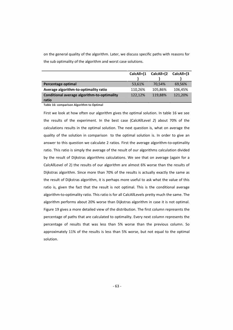
- 63 -

on the general quality of the algorithm. Later, we discuss specific paths with reasons for

the sub optimality of the algorithm and worst case solutions.

CalcAll={1}

CalcAll={2}

CalcAll={3}

Percentage optimal 53,61% 70,54% 69,56% Average algorithm-to-optimality ratio 110,26% 105,86% 106,45% Conditional average algorithm-to-optimality ratio

122,12% 119,88% 121,20%

Table 16: comparison Algorithm to Optimal

First we look at how often our algorithm gives the optimal solution. In table 16 we see

the results of the experiment. In the best case (CalcAllLevel 2) about 70% of the

calculations results in the optimal solution. The next question is, what on average the

quality of the solution in comparison to the optimal solution is. In order to give an

answer to this question we calculate 2 ratios. First the average algorithm-to-optimality

ratio. This ratio is simply the average of the result of our algorithms calculation divided

by the result of Dijkstras algorithms calculations. We see that on average (again for a

CalcAllLevel of 2) the results of our algorithm are almost 6% worse than the results of

Dijkstras algorithm. Since more than 70% of the results is actually exactly the same as

the result of Dijkstras algorithm, it is perhaps more useful to ask what the value of this

ratio is, given the fact that the result is not optimal. This is the conditional average

algorithm-to-optimality ratio. This ratio is for all CalcAllLevels pretty much the same. The

algorithm performs about 20% worse than Dijkstras algorithm in case it is not optimal.

Figure 19 gives a more detailed view of the distribution. The first column represents the

percentage of paths that are calculated to optimality. Every next column represents the

percentage of results that was less than 5% worse than the previous column. So

approximately 11% of the results is less than 5% worse, but not equal to the optimal

solution.

- 64 -

Figure 19: Distribution of Algorithm Performance

The lower the CalcAllLevel, the faster the algorithm turns to the A*-like algorithm and

the more the algorithm cuts of the solution space. However, as opposed to the A*

Therefore we can expect the algorithm to perform better for higher CalcAllLevels. The

CalcAllLevel thus is a trade-off between solution space and quality. And indeed we see

that going from level 1 to level 2 increases the number of optimal solutions with as

much as 20%, while simultaneously decreasing the ratios. From Table 17 it can be seen

that, although for CalcAllLevel 1 the result is still sub optimal, for the higher CalcAllLevels

the results improve.

Starting Point Destination Optimal CalcAll={1} CalcAll={2} CalcAll={3} (39.466245, -0.340522) (39.467957, -0.337415) 0,451184 0,566487 0,451184 0,451184 Table 17: Example of Quality Increasing with CalcAllLevel

0,0%

10,0%

20,0%

30,0%

40,0%

50,0%

60,0%

70,0%

80,0%

CalcAll={1}

CalcAll={2}

CalcAll={3}

- 65 -

Figure 20: Optimal (Left) versus Suboptimal Solution

The sub optimal solution is actually the result of multiple algorithm characteristics. After

the first regions calculations (in case of CalcAllLevel 1) immediately the A*-like algorithm

is used. Furthermore, the estimation of the distance is quite a lot smaller than the real

distance. Therefore, the choice will always be made for RUs that are further away from

the destination. In this specific example, this leads to the investigation of a region that is

not used in the shortest path. However, the fact that a RU can be part of two different

regions when it is a border point, creates a path from starting point to destination

anyway. At the level m controller, the algorithm is programmed to finish the calculations

as soon as there is a path from starting point to destination. These characteristics

combined give the sub optimal solution in the previous example. Therefore we decide to

alter the algorithm slightly. The new algorithm will only finish at the level m controller

once there are no more border points within its region that it wants to investigate. This

should give improved results at the cost of calculation time.

CalcAll={1}

CalcAll={2}

CalcAll={3}

Percentage optimal 65,92% 73,73% 72,66% Average algorithm-to-optimality ratio 105,67% 105,06% 105,11% Conditional average algorithm-to-optimality ratio

116,63% 119,28% 118,71%

Table 18: Comparison Algorithm to Optimal 2

- 66 -

Indeed we see that this change gives an improvement both in the percentage of optimal

results and in the deviation of our algorithm results in comparison to the optimal

solution. Still, even in the improved version of the algorithm, the result for the

CalcAllLevel 2 is more often optimal than the result for the CalcAllLevel 3. We check how

often a lower CalcAllLevel produces better results than a higher CalcAllLevel. From Table

19 we see that this actually occurs quite a lot. Especially the CalcAllLevel 3 performs very

bad. This is not what we expected, since we only anticipated improvements at higher

levels.

1>2 2>3 1&2>3

Algorithm 2,82% 4,87% 2,85% Improved Algorithm 0,54% 1,33% 0,51% Table 19: CalcAllLevels compared

The tool and the test case presented in this chapter gave us the opportunity to review

the algorithm. As it turned out, the characteristics of the algorithm made sub optimal

solutions quite common. A short evaluation provided opportunities for improvement,

still almost 30% of all paths are sub optimal and more extensive research has to be

conducted to find the nature of these non-anticipated results.

- 67 -

5. Towards a Dynamic Algorithm

The algorithm we propose is for the relatively simple static situation. More challenges

arise when creating proper rules for the dynamic situation. Especially because there is

the need to control many vehicles at the same time, the question whether to reroute or

not cannot be answered too often. In this part we give some topics on which future

research could focus. A sort of brainstorm into the possibilities of the dynamic

algorithm, based on the experiences with the static algorithm. The ideas in this chapter

should thus not be viewed as perfect solutions to the problem, but rather as possibilities

for future researchers to explore these areas.

The time dependency of the system can be solved relatively easy. There are different

types of methods that can be used to predict the travel time over an arc, but the so

called BPR (bureau of public roads, creator of the functions) functions are probably the

most used and have the following form:

The final travel time ( is composed of the free flow time ( ) multiplied by a factor

based on the number of cars ( ) and the capacity of the road ( . The coefficients

and often have values of around 0.15 and 4 respectively and control the shape of the

function (Spiess, 1990). Since the number of cars arriving at any moment is stored at the

RU and the distributed system requires an information exchange at every calculation,

the variables are easily filled in.

Difficulties arise however because these formulas assume one steady state travel time,

while in reality you would calculate different times for every new request. The sequence

of cars arriving at the RU is not necessarily the same as the sequence in which the cars

were planned. Therefore, if a vehicle arrives earlier than expected, the travel time over

the arc will always be shorter than expected too, while a vehicle that arrives later than

expected will always take a longer time. This thus will lead to an increase of the

difference between planning and realization. Too minimize this effect the coefficients

and should be chosen such that the differences in travel times between situations

- 68 -

with a different number of vehicles on the arc are smallest. Luckily, time penalties on

busy roads will be much smaller in automated systems than in non-automated systems,

which will justify this decision.

The second problem in the dynamic situation is stochasticity. If the travel time would

just be stochastic and not time-varying, then the calculation of the shortest path based

on the expected values of the travel times is usually considered the best approach

(Miller-Hooks & Mahmassani, 2000). However, imagine the case of an accident that has

blocked the road. Emergency services are working to clear the area but no one knows

for sure when they will finish. At the time of an arriving car, there is only a 10% chance

that the road is cleared again and the traffic is moving at its normal speed of 130 km/h.

This will create an expected travel speed of 13 km/h.

The main reason we cannot search bi-directional is that we need the travel time to a RU

to know the speed at which to travel an RU, because the system is time-varying. There is

no possibility however, that you will arrive at the next RU with a speed of 13 km/h.

next RU, we arrive there with a speed of 130 km/h. This is the conditional expected

value under the condition that you can drive and is therefore the most useful. Most

likely in this case, the road will not be available at all, though. The next question should

thus be whether to use the conditional expected value in the first place, or not. A

possibility might be to use a personal risk acceptance level that every driver can enter. If

the probability that the vehicle cannot enter the road is larger than the risk acceptance

level, then the road will be regarded as completely unavailable to that vehicle.

In the two situations described above, we have two major and obvious risks, i.e. that the

difference between the planning and realization become too large and that the road will

be unavailable anyway. In these cases we need rerouting. We reviewed the topic of

rerouting in chapter two and concluded that most systems found in literature reconsider

the path at every node. Since we expect that to be too time consuming for the GAT

system, we propose four other events to initiate the rerouting in the GATS algorithm.

- 71 -

References Astrachan, O. (2003). Bubble Sort: An Archaeological Algorithmic Analysis. Reno.

Barrett, C., Bisset, K., Holzer, M., Konjevod, G., Marathe, M., & Wagner, D. (2006). Implementations of routing algorithms for transportation networks.

Ben-Akiva, M., & Lerman, S. R. (1985). Discrete Choice Analysis: Theory and Application to Travel Demand. MA: MIT Press.

Cambridge Systematics, Inc. (2008). Crashes vs. Congestion - What´s the Cost to Society?

Dean, B. (2004). Shortest Paths in FIFO Time-Dependent Networks: Theory and Algorithms. MIT, Cambridge MA.

Fu, L., Sun, D., & Rilett, L. (2006). Heuristic Shortest Path Algorithms for Transportation Applications: State of the Art. Computers & Operations Research , 33, 3324-3343.

Gao, S. (2005). Optimal Adaptive Routing and Traffic Assignment in Stochastic Time-Dependent Networks. PhD dissertation, Massachusetts Institute of Technology .

Gao, S., & Chabini, I. (2006). Optimal routing policy problems in stochastic time-dependent networks. Transportation Research Part B , Vol. 40, 93-122.

Giret, A., & Botti, V. (2004). Holons and agents. Journal of Intelligent Manufacturing , 15, 645-659.

Google. (2008). Google Maps. Retrieved from http://maps.google.es/maps?f=d&saddr=A-62+%4040.617040,+-6.512780&daddr=42.212245,-8.712158&t=p&z=7

Hasselberg, S. (2000). Some Results on Heuristical Algorithms for Shortest Path Problems in Large Road Networks. PhD-Thesis, Köln University .

Klunder, G., & Post, H. (2006). The Shortest Path Problem on Large-Scale Real Road Networks. Networks , Vol 48, 182-194.

Labiale, G. (1997). Ergonomics and safety of intellegent driver interfaces. USA: Lawrence Erlbaum Associates, Inc.

Lamont, M. (2008). Sorting Algorithms. Retrieved from http://linux.wku.edu/~lamonml/algor/sort/sort.html

http://maps.google.es/maps?f=d&saddr=A-62+%4040.617040,+

http://linux.wku.edu/~lamonml/algor/sort/sort.html

- 72 -

Maerivoet, S., & De Moor, B. (2008). Transportation Planning and Traffic Flow Models. Arxiv physics and Society.

Mahmassani, H., & and Jayakrishnan, R. (1991). System performance and user response under real-time information in a congested traffic corridor. Transportation Research A , Vol. 25, 293 307.

Miller-Hooks, E. D., & Mahmassani, H. S. (2000). Least Expected Time Paths in Stochastic, Time-varying Transportation Networks. Transportation Science , Vol 34, No. 2.

Miller-Hooks, E., & Mahmassani, H. (2003). Path comparisons for a priori and time-adaptive decisions in stochastic, time-varying networks. European Journal of Operational Research , Vol 146, 67-82.

Musser, D. (1997). Introspective Sorting and Selection Algorithms. Software - Practice and Experience , Vol 27, 983-993.

Noy, Y. (1990). Selective Attention with Auxiliary Automobile Displays. Proceedings of Human Factors Society 34th annual meeting.

Pallottino, S. (1984). Shortest-Path Methods: Complexity, Interrelations and New Propositions. Networks , Vol 14, 257-267.

Pape, U. (1974). Implementation and Efficiency of Moore Algorithms for the Shortest Root Problem. Mathematical Programming , 7.

Russel, S., & Norvig, P. (2003). Artificial Intelligence. A Modern Approach. NJ: Prentice Hall.

Salido, M., & Giret, A. (2008). Feasible Distributed CSP Models for Scheduling Problems. Engineering Application of Artificial Intelligence .

Sedgewick, R. (1987). Implementing Quicksort Programs. Communications of the ACM , Vol 21, 847-857.

Sinnott, R. (1984). Virues of the Haversine. Sky and Telescope , Vol 68, No. 2, 159.

Spiess, H. (1990). Conical Volume-Delay Functions. Transportation Science , Vol 24, No. 2.

Veness, C. (2008). Movable Type. Retrieved from Calculate distance, bearing and more between two Latitude/Longitude points: http://www.movable-type.co.uk/scripts/latlong.html

http://www.movable

- 73 -

Versteegh, F., Salido, M., & Giret, A. (2007). A Distributed Shortest Path Algorithm for Global Automated Transport System. Technical Report, Technical University of Valencia.

Wagner, D., & Willhalm, T. (2006). Speed-Up Techniques for Shortest-Path Computations. Karlsruhe.

Weisstein, E. W. (2008). Spherical Trigonometry. Retrieved from MathWorld - A Wolfram Web Resource: http://mathworld.wolfram.com/SphericalTrigonometry.html

Wikipedia. (2008). Convex_set. Retrieved from wikipedia.org: http://en.wikipedia.org/wiki/Convex_set

Wikipedia. (2008). Domain_name_system. Retrieved from Wikipedia.org: http://en.wikipedia.org/wiki/Domain_name_system

Wikipedia. (2008). Earth Radius. Retrieved from Wikipedia.org: http://en.wikipedia.org/wiki/Earth_radius

Wikipedia. (2008). Haversine_Formula. Retrieved from Wikipedia.org: http://en.wikipedia.org/wiki/haversine_formula

Wikipedia. (2008). Quicksort. Retrieved from Wikipedia.org: http://en.wikipedia.org/wiki/quicksort

Wikipedia. (2008). Shortest_Path_Problem. Retrieved from Wikipedia.org: http://en.wikipedia.org/wiki/Shortest_path_problem

Wikipedia. (2008). Sorting_Algorithms. Retrieved from Wikipedia.org: http://en.wikipedia.org/wiki/Sorting_Algorithms

Wikipedia. (2008). Uniform-Cost_Search. Retrieved from Wikipedia.org: http://en.wikipedia.org/wiki/uniform-cost_search

Wikipedia. (2008). Use_Case. Retrieved from Wikipedia.org: http://en.wikipedia.org/use_case

Wood, M. F., & DeLoach, S. A. (2000). An Overview of the Multiagent Systems Engineering Methodology. Proceedings of the First International Workshop on Agent-Oriented Software .

Yang, X., & Recker, W. (2006). Modeling Dynamic Vehicle Navigation in a Self-Organizing, Peer-to-Peer, Distributed Traffic Information System. Journal of Intelligent Transportation Systems , Vol. 10, 185 204.

http://mathworld.wolfram.com/SphericalTrigonometry.html

http://en.wikipedia.org/wiki/Convex_set

http://en.wikipedia.org/wiki/Domain_name_system

http://en.wikipedia.org/wiki/Earth_radius

http://en.wikipedia.org/wiki/haversine_formula

http://en.wikipedia.org/wiki/quicksort

http://en.wikipedia.org/wiki/Shortest_path_problem

http://en.wikipedia.org/wiki/Sorting_Algorithms

http://en.wikipedia.org/wiki/uniform-cost_search

http://en.wikipedia.org/use_case

- 74 -

Yue, H., & Shao, C. (2007). Study on the Application of A* Shortest Path Search Algorithm in Dynamic Urban Traffic. Proceedings of the Third International Conference on Natural Computation.

Zelinkovsky, R. (1994). Retrieved 04 2008, from http://www.global-transportation.com

Zhan, F. (1997). Three Fastest Shortest Path Algorithms on Real Road Networks: Data Structures and Procedures. Journal of Geographic Information and Decision Analysis , Vol 1, 69-82.

Zhan, F., & Noon, C. (1998). Shortest Path Algorithms: an Evaluation using Real Road Networks. Transportation Science , Vol 32, No.1.

http://www.global-transportation.com

- 75 -

Appendices

A. MaSE Framework

Send/ReceiveNeighbourInformation

Estimate aLowerbound to the

Traveltime orDistance Left

Decide on the NextRegion to Start

Exploring

Store Car SpecificTravel TimeInformation

Create shortest path

Get vehicle from Ato B

Find Informationabout Border to

Border Time

Convert TravelDistance to Travel

Time

Finding Possible ArcDistances

Calculate ShortestPath

Find Country MaxSpeed

Find Road MaxSpeed

Find Vehicle MaxSpeed

Inform LowerRegions/Ru of

Arrival of Vehicle

Store Arriving Cars

Delete UselessInformation

Holon lvl 2 RUHolon lvl 1 Car

Find Nearest Neighbour with A and B in samelevel m region until the destination is found

Send Car and DestinationInformation

Send Car and Destination Information

Request NearestNeighbour Information

Send Nearest Neighbour Information

Send Car and Destination InformationAccompanied by its Border InformationRequest Nearest

Neighbour Information Request NearestNeighbour Information Send Nearest Neighbour Information


Holon lvl m

Send Car and Destination InformationAccompanied by its Border InformationRequest Nearest

Neighbour Information Request NearestNeighbour Information




Request NearestNeighbour Information Request Nearest

Neighbour Information Send Nearest Neighbour Information


Request NearestNeighbour Information Send Nearest Neighbour Information



Request NearestNeighbour Information Send Nearest Neighbour Information




Return Arcs

Pallottoni Algorithm

Holon lvl 2 RUHolon lvl 1 Car

Inform the Rus of the Arrival of a Vehicle

Holon lvl mInform of Arrival of Car

from specific BorderPoint

Inform of Arrival of Carfrom specific BorderPoint


Inform of Arrival of Car




Inform of Arrival of CarInform of Arrival of Car

Inform of Arrival of CarInform of Arrival of CarInform of Arrival of Car



Send Travel Information to Car

Return Info

Return InfoReturn Info

Return Info

Return InfoReturn Info

Send Travel Information to CarSend Travel Information to Car

Send Travel Information to Car

- 78 -

D. Static Distributed Algorithm Classes

-Location : int-LvL1Controller : LvlController-Arc : Arc-Arriving Cars : Car

RU

-RULocation1 : RU-RULocation2 : RU-ArcLength : double-MaxSpeed : double-Country : int-AvailabilityToVehicle : int

Arc

-Location : string-LvL : int-RUs : RU-LvLDControllers : LvlController-Borders : RU

LvlController

-LicencePlate : string-CarType-RequestType-AccelerationType-MaxSpeed : double-StartLocation : RU-Destination : RU-ShortestPath : RU

Car

+LowSpeedVehicle = 1+Car = 2+SmallTruck = 3+LargeTruck = 4

«enumeration»CarType

- 79 -

E. Static Distributed Algorithm Tasks

Idle

Receive(newDestination(CarCharacteristics))

Car

Role: RU, Task: Process New Destination

Find Lvl1C

Send(newDestination(CarCharacteristics))

Figure 23: Task Diagram 1

Idle FilterPossibleArcsReceive(newRequest(CarCharacteristics)

Lvl 1Ctrl

CalculateTravelTimes

[Request=Time]/Send(Neighbours(Location,Distance))

[Request=Distance]/Send(Neighbours(Location,Distance))

Send(Neighbours(Location,TravelTime))

Role: RU, Task: Return Arc Travel Times


- 80 -

Idle AddRUsToProperQueues


RU

Wait

Role: Lvl1Cntr, Task: Calculate shortest path

[size(Q1,Q2)>0]/Pick(RU,Q1,Q2)

Receive(Neighbours(Location,TravelTime))

Send(Request(CarCharacteristics))

FindBorderPoints(RU)

EvaluateInfo[Neighbour<>Destination]

[size(Q1,Q2)=0 ANDDestination<>Found]/Send

(BorderPoints(Location,TravelTime),newDestination(CarCharacteristics))

[Neighbour=Destination]

Mark DestinationAs Found

[size(Q1,Q2)=0 AND DestinationFound]]InformRUOfArrivalVehicle


Idle AddRUsToProperQueues


LvL2C

Wait

Role: Lvl1Cntr, Task: Calculate shortest path

[size(Q1,Q2)>0]/Pick(RU,Q1,Q2)

Receive(Neighbours(Location,TravelTime))

Send(Request(CarCharacteristics))

FindBorderPoints(RU)

EvaluateInfo[Neighbour<>Destination]

[size(Q1,Q2)=0 ANDDestination<>Found]/Send

(BorderPoints(Location,TravelTime),newDestination(CarCharacteristics),

DestinationFound())

[Neighbour=Destination]

Mark DestinationAs Found


- 81 -

Idle FindBorderPointsOfExploredRegion


LvlDC

Wait

Role: LowerLvlCntr, Task: Calculate shortest path

Pass(newDestination(CarCharacteristics),StartPoint(Location,

TravelTime))Receive(Neighbours

(Location,TravelTime))

[size(listBordersUnvisited)>0]/Send(Request(CarType,

CarChar,RequestType))

CalculateToLvlDown

(StartPoint)

EvaluateInfo

[Neighbour<>Destination]/Send((Neighbours


[size(listRUunvisited)=0]/Send(newDestination(CarCharacteristics))

[Neighbour=Destination]/Send(ArrivalInformation(CarCharacteristics))

InformRUOfArrivalVehicle


Idle

FindBorderPointsOfExploredRegion

Receive(newDestination(CarCharacteristics),

StartPoint(Locations,TravelTime))

LvlUC

Wait

Role: LowerLvlCntr, Task: Calculate shortest path




[size(listBordersUnvisited)>0]/Send(Request(CarCharacteristics)

CalculateToLvlDown

(StartPoint)

EvaluateInfo[Neighbour<>Destination]/

Send((Neighbours(Location,TravelTime))

[size(listRUunvisited)=0]/Send(newDestination(CarCharacteristics))

[Neighbour<>Destination]/Send(newDestination(CarCharacteristics))


- 82 -

Idle FindBestBorderPoints


LvlDC

Wait

Role: HigherLvlCntr, Task: Calculate shortest path




[BorderInRegion=True]/Send(Request(CarType,

CarChar,RequestType))

CalculateToLvlDown

(StartPoint)

EvaluateInfo

[Neighbour<>Destination]/Send((Neighbours


[BorderInRegion=False]/Send(newDestination(CarCharacteristics))

[Neighbour=Destination]/Send(ArrivalInformation(CarCharacteristics))

InformRUOfArrivalVehicle


Idle

FindBestBorderPoints

Receive(newDestination(CarCharacteristics),

StartPoint(Location,TravelTime))

LvlUC

Wait

Role: HigherLvlCntr, Task: Calculate shortest path




[BorderInRegion=True]/Send(Request(CarType,

CarChar,RequestType),StarPoint(Location,TravelTime))

CalculateToLvlDown

(StartPoint)

EvaluateInfo[Neighbour<>Destination]/

Send((Neighbours(Location,TravelTime))

[BorderInRegion=False]/Send(newDestination(CarCharacteristics))

[Neighbour<>Destination]/Send(newDestination(CarCharacteristics))


A Holonic Architecture for the Global Automated ...

Documents

Transcript of A Holonic Architecture for the Global Automated ...