Legalized Recreational Marijuana, Automated Electric ...
256
Legalized Recreational Marijuana, Automated Electric Vehicles and Support for the New Mexico State Police Jeremy Vaughan President
-
Upload
khangminh22 -
Category
Documents
-
view
2 -
download
0
Transcript of Legalized Recreational Marijuana, Automated Electric ...

Legalized Recreational Marijuana,
Automated Electric Vehicles
and Support for the New Mexico State Police
Jeremy VaughanPresident


PREPARED BY:
ROCKY MOUNTAIN HIDTA
STRATEGIC INTELLIGENCE UNIT

DRAFT
The Legalization of Marijuana in Colorado: The Impact Vol. 5/October 2017
Table of Contents P a g e | i
Table of Contents
Executive Summary ............................................................................................ 1 Purpose ..................................................................................................................................1
Introduction .......................................................................................................... 7
Purpose ..................................................................................................................................7
The Debate ............................................................................................................................8
Background ...........................................................................................................................8
Preface ....................................................................................................................................8
Colorado’s History with Marijuana Legalization ...........................................................9 Medical Marijuana 2000-2008 .................................................................................................... 9
Medical Marijuana Commercialization and Expansion 2009-Present ............................... 10
Recreational Marijuana 2013-Present...................................................................................... 11
SECTION 1: Impaired Driving and Fatalities ............................................ 13
Some Findings ....................................................................................................................13
Differences in Data Citations ............................................................................................14
Definitions by Rocky Mountain HIDTA ........................................................................14
Data for Traffic Deaths ......................................................................................................15 Total Number of Statewide Traffic Deaths ........................................................................... 15
Traffic Deaths Related to Marijuana When a Driver Tested Positive for Marijuana ..... 16
Percent of All Traffic Deaths that were Marijuana-Related when a Driver Tested Positive
for Marijuana ............................................................................................................................ 17
Average Number of Traffic Deaths Related to Marijuana when a Driver Tested Positive
for Marijuana ............................................................................................................................ 18
Drug Combinations for Drivers who Tested Positive for Marijuana, 2016 .................... 18
Traffic Deaths Related to Marijuana When an Operator Tested Positive for Marijuana.19
Percent of All Traffic Deaths that were Marijuana-Related when an Operator Tested
Positive for Marijuana ............................................................................................................. 20
Average Number of Traffic Deaths Related to Marijuana when an Operator Tested
Positive for Marijuana ............................................................................................................. 21
Drug Combinations for Operators who Tested Positive for Marijuana, 2016 ................. 21
Data for Impaired Driving ................................................................................................22 Number of Positive Cannabinoid Screens ............................................................................ 22
ChemaTox and Colorado Department of Public Health and Environment (Data
Combined 2009-2013) ........................................................................................................ 23
ChemaTox Data Only (2013-May2016) ................................................................................. 23

DRAFT
The Legalization of Marijuana in Colorado: The Impact Vol. 5/October 2017
Table of Contents P a g e | ii
Colorado State Patrol Number of Drivers Under the Influence of Drugs (DUIDs) ....... 24
Marijuana as a Percent of All DUI and DUIDs .................................................................... 25
Denver Police Department Percent of DUIDs Involving Marijuana ................................ 26
Larimer County Sheriff’s Office Percent of DUIDs Involving Marijuana........................ 26
Total Number of Accidents in Colorado .............................................................................. 27
Related Costs ......................................................................................................................27
Case Examples ....................................................................................................................28
Sources .................................................................................................................................31
SECTION 2: Youth Marijuana Use ............................................................... 33
Some Findings ....................................................................................................................33
Surveys NOT Utilized .......................................................................................................33 Healthy Kids Colorado Survey (HKCS) ............................................................................... 33
Current Marijuana Use for High School and Middle School Students in Colorado.34
Monitoring the Future (MTF) Study ..................................................................................... 35
Centers for Disease Control Youth Risk Behavior Survey (YRBS) ................................... 35
2015 YRBS Participation Map .......................................................................................... 35
Use Data ..............................................................................................................................36 Youth Ages 12 to 17 Years Old ............................................................................................... 36
Average Past Month Use of Marijuana Youth Ages 12 to 17 Years Old .................... 36
Past Month Marijuana Use Youth Ages 12 to 17 Years Old ........................................ 36
Prevalence of Past 30-Day Marijuana Use Youth Ages 12 to 17 Years Old ............... 37
Past Month Usage, 12 to 17 Years Old, 2014/2015......................................................... 38
Average Past Month Use Youth Ages 12 to 17 Years Old, 2014/2015 ........................ 39
Past Month Marijuana Use Youth Ages 12 to 17 Years Old, 2014/2015 ..................... 39
Colorado Probation Percent of All Urinalysis Tests Positive for Marijuana
Youth Ages 10 to 17 Years Old ........................................................................................ 40
School Data .........................................................................................................................41 Impact on School Violation Numbers ................................................................................... 41
All Drug Violations, 2015-2016 School Year .................................................................. 41
Drug-Related Suspensions/Expulsions .......................................................................... 42
Percent of Total Referrals to Law Enforcement in Colorado....................................... 42
Number of Reported School Dropouts ........................................................................... 43
Colorado School Resource Officer Survey .....................................................................43 Impact on Marijuana-Related Incidents, 2017 ...................................................................... 44 Predominant Marijuana Violations, 2017 ............................................................................. 44
Student Marijuana Source, 2017 ............................................................................................. 45
School Counselor Survey ..................................................................................................45 Impact on Marijuana-Related Incidents, 2015 ...................................................................... 46
Predominant Marijuana Violations, 2015 ............................................................................. 46
Student Marijuana Source, 2015 ............................................................................................. 47
Case Examples ....................................................................................................................47

DRAFT
The Legalization of Marijuana in Colorado: The Impact Vol. 5/October 2017
Table of Contents P a g e | iii
Some Comments from School Resource Officers ................................................................ 49
Some Comments from School Counselors ........................................................................... 51
Sources .................................................................................................................................53
SECTION 3: Adult Marijuana Use ............................................................... 55
Some Findings ....................................................................................................................55
Use Data ..............................................................................................................................56 College Age 18 to 25 Years Old .............................................................................................. 56
Average Past Month Use of Marijuana College Age 18 to 25 Years Old ................... 56
Past Month Marijuana Use College Age 18 to 25 Years Old ....................................... 56
Prevalence of Past 30-Day Marijuana Use College Age 18 to 25 Years Old .............. 57
Past Month Usage, 18 to 25 Years Old, 2014/2015......................................................... 58
Average Past Month Use College Age 18 to 25 Years Old, 2014/2015 ....................... 59
Past Month Marijuana Use College Age 18 to 25 Years Old, 2014/2015 .................... 59
Adults Age 26+ Years Old ....................................................................................................... 60
Average Past Month Use of Marijuana College Ages 26+ Years Old......................... 60
Past Month Marijuana Use Adults Age 26+ Years Old ................................................ 60
Prevalence of Past 30-Day Marijuana Use College Adults Age 26+ Years Old ........ 61
Past Month Usage, 26+ Years Old, 2014/2015 ................................................................ 62
Average Past Month Use Adults Ages 26+ Years Old, 2014/2015 .............................. 63
Past Month Marijuana Use Adults Ages 26+ Years Old, 2014/2015 ........................... 63
Colorado Adult Marijuana Use Demographics ................................................................... 64
Case Examples ....................................................................................................................64
Sources .................................................................................................................................66
SECTION 4: Emergency Department and Hospital Marijuana-Related
Admissions ................................................................................ 67 Some Findings ....................................................................................................................67
Definitions ...........................................................................................................................68
Emergency Department Data ...........................................................................................68 Colorado Department of Public Health and Environment ................................................ 68
Average Emergency Department Rates Related to Marijuana ................................... 69
Emergency Department Rates Related to Marijuana ................................................... 70
Emergency Department Visits Related to Marijuana ................................................... 71
Hospitalization Data ..........................................................................................................72 Colorado Department of Public Health and Environment ................................................ 72
Average Hospitalization Rates Related to Marijuana .................................................. 72
Hospitalization Rates Related to Marijuana .................................................................. 73
Average Hospitalizations Related to Marijuana ........................................................... 74
Hospitalizations Related to Marijuana ........................................................................... 74
Additional Sources................................................................................................................... 75

DRAFT
The Legalization of Marijuana in Colorado: The Impact Vol. 5/October 2017
Table of Contents P a g e | iv
Children’s Hospital Marijuana Ingestion Among Children Under 9 Years Old ...... 75
Cost ......................................................................................................................................75
Case Examples ....................................................................................................................76
Sources .................................................................................................................................80
SECTION 5: Marijuana-Related Exposure ................................................. 81 Some Findings ....................................................................................................................81
Definitions ...........................................................................................................................81
Data ......................................................................................................................................82 Average Number of Marijuana-Related Exposures, All Ages ........................................... 82
Marijuana-Related Exposures ................................................................................................ 82
Marijuana-Related Exposures by Age Range ...................................................................... 83
Average Percent of All Marijuana-Related Exposures, Children Ages
0 to 5 Years Old ........................................................................................................................ 83
Number of Marijuana Only Exposures Reported ............................................................... 84
Case Examples ....................................................................................................................84
Sources .................................................................................................................................85
SECTION 6: Treatment ................................................................................... 87 Some Findings ....................................................................................................................87
Data ......................................................................................................................................87 Treatment with Marijuana as Primary Substance Abuse, All Ages ................................. 87
Drug Type for Treatment Admissions, All Ages ................................................................. 88
Percent of Marijuana Treatment Admissions by Age Group ............................................ 89
Marijuana Treatment Admissions Based on Criminal Justice Referrals .......................... 90
Comments from Colorado Treatment Providers ..........................................................90
Case Examples ....................................................................................................................91
Sources .................................................................................................................................92
SECTION 7: Diversion of Colorado Marijuana ......................................... 93 Some Findings ....................................................................................................................93
Definitions ...........................................................................................................................94
Data on Marijuana Investigations ...................................................................................95 RMHIDTA Colorado Task Forces: Marijuana Investigation Seizures.............................. 95
RMHIDTA Colorado Task Forces: Marijuana Investigative Plant Seizures .................... 96
RMHIDTA Colorado Task Forces: Marijuana Investigative Felony Arrests ................... 96
Data on Highway Interdictions .......................................................................................97 Average Colorado Marijuana Interdiction Seizures ........................................................... 97
Colorado Marijuana Interdiction Seizures ........................................................................... 98
Average Pounds of Colorado Marijuana from Interdiction Seizures ............................... 98
States to Which Colorado Marijuana Was Destined, 2016 ................................................. 99

DRAFT
The Legalization of Marijuana in Colorado: The Impact Vol. 5/October 2017
Table of Contents P a g e | v
Top Three Cities for Marijuana Origin ................................................................................. 99
Case Examples of Investigations ...................................................................................100
Case Examples of Interdictions ......................................................................................103
Sources ...............................................................................................................................107
SECTION 8: Diversion by Parcel ................................................................ 109 Some Findings ..................................................................................................................109
Data from U.S. Postal Service .........................................................................................109 Average Number of Parcels Containing Marijuana Mailed from Colorado to Another
State .......................................................................................................................................... 109
Parcels Containing Marijuana Mailed from Colorado to Another State ........................ 110
Average Pounds of Colorado Marijuana Seized by the U.S. Postal Inspection
Service ...................................................................................................................................... 110
Pounds of Colorado Marijuana Seized by the U.S. Postal Inspection Service .............. 111
Number of States Destined to Receive Marijuana Mailed from Colorado .................... 111
Private Parcel Companies ...............................................................................................112
Case Examples ..................................................................................................................113
Sources ...............................................................................................................................115
SECTION 9: Related Data ............................................................................ 117 Topics .................................................................................................................................117
Some Findings ..................................................................................................................117
Crime .................................................................................................................................118 Colorado Crime ...................................................................................................................... 118
City and County of Denver Crime ...................................................................................... 119
Crime in Denver ..................................................................................................................... 120
Denver Police Department Unlawful Public Display/Consumption of Marijuana ...... 120
Boulder Police Department Marijuana Public Consumption Citations ......................... 121
Case Examples ........................................................................................................................ 121
Revenue .............................................................................................................................124 Colorado’s Statewide Budget, Fiscal Year 2017 ................................................................. 124
Total State Revenue from Marijuana Taxes, Calendar Year 2016 ................................... 124
Case Example.......................................................................................................................... 125
Event Planners’ Views of Denver ..................................................................................126 Negative Meeting Planner Perceptions, 2014..................................................................... 126
Homeless ...........................................................................................................................128
Suicide Data ......................................................................................................................130 Average Toxicology of Suicides Among Adolescents Ages 10 to 19 Years Old (With
Known Toxicology) ......................................................................................................130
Average Toxicology Results by Age Group, 2013-2015 ...............................................131
THC Potency .....................................................................................................................132
DRAFT
The Legalization of Marijuana in Colorado: The Impact Vol. 5/October 2017
Table of Contents P a g e | vi
National Average THC Potency Submitted Cannabis Samples ...................................... 132
National Average THC Potency Submitted Hash Oil Samples....................................... 133
Alcohol Consumption .....................................................................................................134 Colorado Average Consumption of Alcohol ..................................................................... 134
Colorado Consumption of Alcohol ..................................................................................... 134
Medical Marijuana Registry ...........................................................................................135 Percent of Medical Marijuana Patients Based on Reporting Conditions, 2016 ............. 136
Colorado Licensed Marijuana Businesses as of August 1st, 2017 ..............................137
Business Comparisons, June 2017 ..................................................................................137 Colorado Business Comparisons, June 2017 ...................................................................... 137
Demand and Market Size ...............................................................................................138 Demand ................................................................................................................................... 138
Market Size ............................................................................................................................. 138
Marijuana Enforcement Division Reported Sales of Marijuana in Colorado..........139
2017 Price of Marijuana ...................................................................................................139
Local Response to Medical and Recreational Marijuana in Colorado .....................140 2016 Local Jurisdiction Licensing Status ............................................................................. 142
Sources ...............................................................................................................................143
SECTION 10: Reference Materials ............................................................. 147 Reports and Articles ........................................................................................................147
Impaired Driving ................................................................................................................... 147
Youth Marijuana Use ............................................................................................................. 151
Adult Marijuana Use ............................................................................................................. 152
Emergency Department and Hospital Marijuana-Related Admissions......................... 155
Marijuana-Related Exposure ................................................................................................ 157
Treatment ................................................................................................................................ 157
Related Data ............................................................................................................................ 158
Sources ...............................................................................................................................163

DRAFT
The Legalization of Marijuana in Colorado: The Impact Vol. 5/October 2017
Executive Summary P a g e | 1
Executive Summary
Purpose
Rocky Mountain High Intensity Drug Trafficking Area (RMHIDTA) is tracking the
impact of marijuana legalization in the state of Colorado. This report will utilize,
whenever possible, a comparison of three different eras in Colorado’s legalization
history:
2006 – 2008: Medical marijuana pre-commercialization era
2009 – Present: Medical marijuana commercialization and expansion era
2013 – Present: Recreational marijuana era
Rocky Mountain HIDTA will collect and report comparative data in a variety of
areas, including but not limited to:
Impaired driving and fatalities
Youth marijuana use
Adult marijuana use
Emergency room admissions
Marijuana-related exposure cases
Diversion of Colorado marijuana
This is the fifth annual report on the impact of legalized marijuana in Colorado. It is
divided into ten sections, each providing information on the impact of marijuana
legalization. The sections are as follows:
Section 1 – Impaired Driving and Fatalities:
Marijuana-related traffic deaths when a driver was positive for marijuana more
than doubled from 55 deaths in 2013 to 125 deaths in 2016.
Marijuana-related traffic deaths increased 66 percent in the four-year average
(2013-2016) since Colorado legalized recreational marijuana compared to the
four-year average (2009-2012) prior to legalization.
o During the same time period, all traffic deaths increased 16 percent.

DRAFT
The Legalization of Marijuana in Colorado: The Impact Vol. 5/October 2017
Executive Summary P a g e | 2
In 2009, Colorado marijuana-related traffic deaths involving drivers testing
positive for marijuana represented 9 percent of all traffic deaths. By 2016, that
number has more than doubled to 21 percent.
Section 2 – Youth Marijuana Use:
Youth past month marijuana use increased 12 percent in the three-year average
(2013-2015) since Colorado legalized recreational marijuana compared to the
three-year average prior to legalization (2010-2012).
The latest 2014/2015 results show Colorado youth ranked #1 in the nation for past
month marijuana use, up from #4 in 2011/2012 and #14 in 2005/2006.
Colorado youth past month marijuana use for 2014/2015 was 55 percent higher
than the national average compared to 39 percent higher in 2011/2012.
Section 3 – Adult Marijuana Use:
College age past month marijuana use increased 16 percent in the three-year
average (2013-2015) since Colorado legalized recreational marijuana compared to
the three-year average prior to legalization (2010-2012).
The latest 2014/2015 results show Colorado college-age adults ranked #2 in the
nation for past-month marijuana use, up from #3 in 2011/2012 and #8 in
2005/2006.
Colorado college age past month marijuana use for 2014/2015 was 61 percent
higher than the national average compared to 42 percent higher in 2011/2012.
Adult past-month marijuana use increased 71 percent in the three-year average
(2013-2015) since Colorado legalized recreational marijuana compared to the
three-year average prior to legalization (2010-2012).
The latest 2014/2015 results show Colorado adults ranked #1 in the nation for
past month marijuana use, up from #7 in 2011/2012 and #8 in 2005/2006.
Colorado adult past month marijuana use for 2014/2015 was 124 percent higher
than the national average compared to 51 percent higher in 2011/2012.

DRAFT
The Legalization of Marijuana in Colorado: The Impact Vol. 5/October 2017
Executive Summary P a g e | 3
Section 4 – Emergency Department and Hospital Marijuana-Related Admissions:
The yearly rate of emergency department visits related to marijuana increased 35
percent after the legalization of recreational marijuana (2011-2012 vs. 2013-2015).
Number of hospitalizations related to marijuana:
o 2011 – 6,305
o 2012 – 6,715
o 2013 – 8,272
o 2014 – 11,439
o Jan-Sept 2015 – 10,901
The yearly number of marijuana-related hospitalizations increased 72 percent
after the legalization of recreational marijuana (2009-2012 vs. 2013-2015).
Section 5 – Marijuana-Related Exposure:
Marijuana-related exposures increased 139 percent in the four-year average
(2013-2016) since Colorado legalized recreational marijuana compared to the
four-year average (2009-2012) prior to legalization.
Marijuana-Only exposures more than doubled (increased 210 percent) in the
four-year average (2013-2016) since Colorado legalized recreational marijuana
compared to the four-year average (2009-2012) prior to legalization.
Section 6 – Treatment:
Marijuana treatment data from Colorado in years 2006 – 2016 does not appear to
demonstrate a definitive trend. Colorado averages 6,683 treatment admissions
annually for marijuana abuse.
Over the last ten years, the top four drugs involved in treatment admissions were
alcohol (average 13,551), marijuana (average 6,712), methamphetamine (average
5,578), and heroin (average 3,024).

DRAFT
The Legalization of Marijuana in Colorado: The Impact Vol. 5/October 2017
Executive Summary P a g e | 4
Section 7 – Diversion of Colorado Marijuana:
In 2016, RMHIDTA Colorado drug task forces completed 163 investigations of
individuals or organizations involved in illegally selling Colorado marijuana
both in and out of state.
o These cases led to:
252 felony arrests
7,116 (3.5 tons) pounds of marijuana seized
47,108 marijuana plants seized
2,111 marijuana edibles seized
232 pounds of concentrate seized
29 different states to which marijuana was destined
Highway interdiction seizures of Colorado marijuana increased 43 percent in the
four-year average (2013-2016) since Colorado legalized recreational marijuana
compared to the four-year average (2009-2012) prior to legalization.
Of the 346 highway interdiction seizures in 2016, there were 36 different states
destined to receive marijuana from Colorado.
o The most common destinations identified were Illinois, Missouri, Texas,
Kansas and Florida.
Section 8 – Diversion by Parcel:
Seizures of Colorado marijuana in the U.S. mail has increased 844 percent from
an average of 52 parcels (2009-2012) to 491 parcels (2013-2016) in the four-year
average that recreational marijuana has been legal.
Seizures of Colorado marijuana in the U.S. mail has increased 914 percent from
an average of 97 pounds (2009-2012) to 984 pounds (2013-2016) in the four-year
average that recreational marijuana has been legal.

DRAFT
The Legalization of Marijuana in Colorado: The Impact Vol. 5/October 2017
Executive Summary P a g e | 5
Section 9 – Related Data:
Crime in Denver increased 6 percent from 2014 to 2016 and crime in Colorado
increased 11 percent from 2013 to 2016.
Colorado annual tax revenue from the sale of recreational and medical marijuana
was 0.8 percent of Colorado’s total statewide budget (FY 2016).
As of June 2017, there were 491 retail marijuana stores in the state of Colorado
compared to 392 Starbucks and 208 McDonald’s.
66 percent of local jurisdictions have banned medical and recreational marijuana
businesses.
Section 10 – Reference Materials:
This section lists various studies and reports regarding marijuana.
THERE IS MUCH MORE DATA IN EACH OF THE TEN SECTIONS. THIS PUBLICATION MAY BE
FOUND ON THE ROCKY MOUNTAIN HIDTA WEBSITE; GO TO WWW.RMHIDTA.ORG AND SELECT
REPORTS.

DRAFT
The Legalization of Marijuana in Colorado: The Impact Vol. 5/October 2017
Executive Summary P a g e | 6
THIS PAGE INTENTIONALLY LEFT BLANK

The Legalization of Marijuana in Colorado: The Impact Vol. 5/October 2017
Introduction Page | 7
Introduction
Purpose
The purpose of this annual report is to document the impact of the legalization of
marijuana for medical and recreational use in Colorado. Colorado serves as an
experimental lab for the nation to determine the impact of legalizing marijuana. This is
an important opportunity to gather and examine meaningful data and identify trends.
Citizens and policymakers nationwide may want to delay any decisions on this
important issue until there is sufficient and accurate data to make informed decisions.
The Debate
There is an ongoing debate in this country concerning the impact of legalizing
marijuana. Those in favor argue that the benefits of removing prohibition far outweigh
the potential negative consequences. Some of the cited benefits include:
Eliminate arrests for possession and sale, resulting in fewer people with criminal
records and a reduction in the prison population
Free up law enforcement resources to target more serious and violent criminals
Reduce traffic fatalities since users will switch from alcohol to marijuana, which
does not impair driving to the same degree
No increase in use, even among youth, because of strict regulations
Added revenue generated through taxation
Eliminate the black market
Those opposed to legalizing marijuana argue that the potential benefits of lifting
prohibition pale in comparison to the adverse consequences. Some of the cited
consequences include:
Increase in marijuana use among youth and young adults
Increase in marijuana-impaired driving fatalities
Rise in number of marijuana-addicted users in treatment
Diversion of marijuana

The Legalization of Marijuana in Colorado: The Impact Vol. 5/October 2017
Introduction Page | 8
Adverse impact and cost of the physical and mental health damage caused by
marijuana use
The economic cost to society will far outweigh any potential revenue generated
Background
As of 2016, a number of states have enacted varying degrees of legalized marijuana
by permitting medical marijuana and eight permitting recreational marijuana. In 2010,
legislation was passed in Colorado that included the licensing of medical marijuana
centers (dispensaries), cultivation operations, and manufacturing of marijuana edibles
for medical purposes. In November 2012, Colorado voters legalized recreational
marijuana allowing individuals to use and possess an ounce of marijuana and grow up
to six plants. The amendment also permits licensing marijuana retail stores, cultivation
operations, marijuana edible manufacturers, and testing facilities. Washington voters
passed a similar measure in 2012.
Preface
It is important to note that, for purposes of the debate on legalizing marijuana in
Colorado, there are three distinct timeframes to consider: the early medical marijuana
era (2000-2008), the medical marijuana commercialization era (2009 – current) and the
recreational marijuana era (2013 – current).
2000 – 2008: In November 2000, Colorado voters passed Amendment 20 which
permitted a qualifying patient, and/or caregiver of a patient, to possess up to 2
ounces of marijuana and grow 6 marijuana plants for medical purposes. During
that time there were between 1,000 and 4,800 medical marijuana cardholders and
no known dispensaries operating in the state.
2009 – Current: Beginning in 2009 due to a number of events, marijuana became
de facto legalized through the commercialization of the medical marijuana
industry. By the end of 2012, there were over 100,000 medical marijuana
cardholders and 500 licensed dispensaries operating in Colorado. There were
also licensed cultivation operations and edible manufacturers.

The Legalization of Marijuana in Colorado: The Impact Vol. 5/October 2017
Introduction Page | 9
2013 – Current: In November 2012, Colorado voters passed Constitutional
Amendment 64 which legalized marijuana for recreational purposes for anyone
over the age of 21. The amendment also allowed for licensed marijuana retail
stores, cultivation operations and edible manufacturers. Retail marijuana
businesses became operational January 1, 2014.
Colorado’s History with Marijuana Legalization
Medical Marijuana 2000 – 2008
In November 2000, Colorado voters passed Amendment 20 which permitted a
qualifying patient and/or caregiver of a patient to possess up to 2 ounces of marijuana
and grow 6 marijuana plants for medical purposes. Amendment 20 provided
identification cards for individuals with a doctor’s recommendation to use marijuana
for a debilitating medical condition. The system was managed by the Colorado
Department of Public Health and Environment (CDPHE), which issued identification
cards to patients based on a doctor’s recommendation. The department began
accepting applications from patients in June 2001.
From 2001 – 2008, there were only 5,993 patient applications received and only 55
percent of those designated a primary caregiver. During that time, the average was
three patients per caregiver and there were no known retail stores selling medical
marijuana (dispensaries). Dispensaries were not an issue because CDPHE regulations
limited a caregiver to no more than five patients.
In late 2007, a Denver district judge ruled that CDPHE violated the state’s open
meeting requirement when it set a five-patient-to-one-caregiver ratio and overturned
the rule. That opened the door for caregivers to claim an unlimited number of patients
for whom they were providing and growing marijuana. Although this decision
expanded the parameters, very few initially began operating medical marijuana
commercial operations (dispensaries) in fear of prosecution, particularly from the
federal government.
The judge’s ruling, and caregivers expanding their patient base, created significant
problems for local prosecutors seeking a conviction for marijuana distribution by
caregivers. Many jurisdictions ceased or limited filing those types of cases.

The Legalization of Marijuana in Colorado: The Impact Vol. 5/October 2017
Introduction Page | 10
Medical Marijuana Commercialization and Expansion 2009 – Present
The dynamics surrounding medical marijuana in Colorado began to change
substantially after the Denver judge’s ruling in late 2007, as well as several incidents
beginning in early 2009. All of these combined factors played a role in the explosion of
the medical marijuana industry and number of patients:
At a press conference in Santa Ana, California on February 25, 2009, U.S. Attorney
General Eric Holder was asked whether raids in California on medical marijuana
dispensaries would continue. He responded “No” and referenced the President’s
campaign promise related to medical marijuana. In mid-March 2009, the U.S. Attorney
General clarified the position saying that the Department of Justice enforcement policy
would be restricted to traffickers who falsely masqueraded as medical dispensaries and
used medical marijuana laws as a shield.
Beginning in the spring of 2009, Colorado experienced an explosion to over 20,000
new medical marijuana patient applications and the emergence of over 250 medical
marijuana dispensaries (allowed to operate as “caregivers”). One dispensary owner
claimed to be a primary caregiver to 1,200 patients. Government took little or no action
against these commercial operations.
In July 2009, the Colorado Board of Health, after public hearings, voted to keep the
judge’s ruling of not limiting the number of patients a single caregiver could have.
They also voted to change the definition of a caregiver to a person that only had to
provide medicine to patients, nothing more.
On October 19, 2009, U.S. Deputy Attorney General David Ogden provided
guidelines for U.S. Attorneys in states that enacted medical marijuana laws. The memo
advised to “Not focus federal resources in your state on individuals whose actions are
in clear and unambiguous compliance with existing state law providing for the medical
use of marijuana.”
By the end of 2009, new patient applications jumped from around 6,000 for the first
seven years to an additional 38,000 in just one year. Actual cardholders went from 4,800
in 2008 to 41,000 in 2009. By mid-2010, there were over 900 unlicensed marijuana
dispensaries identified by law enforcement.
In 2010, law enforcement sought legislation to ban dispensaries and reinstate the
one-to-five ratio of caregiver to patient as the model. However, in 2010 the Colorado

The Legalization of Marijuana in Colorado: The Impact Vol. 5/October 2017
Introduction Page | 11
Legislature passed HB-1284 which legalized medical marijuana centers (dispensaries),
marijuana cultivation operations, and manufacturers for marijuana edible products. By
2012, there were 532 licensed dispensaries in Colorado and over 108,000 registered
patients, 94 percent of which qualified for a card because of severe pain.
Recreational Marijuana 2013 – Present
In November of 2012, Colorado voters passed Amendment 64 which legalized
marijuana for recreational use. Amendment 64 allows individuals 21 years or older to
grow up to six plants, possess/use 1 ounce or less, and furnish an ounce or less of
marijuana if not for the purpose of remuneration. Amendment 64 permits marijuana
retail stores, marijuana cultivation sites, marijuana edible manufacturers and marijuana
testing sites. The first retail marijuana businesses were licensed and operational in
January of 2014. Some individuals have established private cannabis clubs, formed co-
ops for large marijuana grow operations, and/or supplied marijuana for no fee other
than donations.
What has been the impact of commercialized medical marijuana and legalized
recreational marijuana on Colorado? Review the report and you decide.
NOTES:
DATA, IF AVAILABLE, WILL COMPARE PRE- AND POST-2009 WHEN MEDICAL MARIJUANA
BECAME COMMERCIALIZED AND AFTER 2013 WHEN RECREATIONAL MARIJUANA BECAME
LEGALIZED.
MULTI-YEAR COMPARISONS ARE GENERALLY BETTER INDICATORS OF TRENDS. ONE-YEAR
FLUCTUATIONS DO NOT NECESSARILY REFLECT A NEW TREND.
PERCENTAGE COMPARISONS MAY BE ROUNDED TO THE NEAREST WHOLE NUMBER.
PERCENT CHANGES ADDED TO GRAPHS WERE CALCULATED AND ADDED BY ROCKY
MOUNTAIN HIDTA.
THIS REPORT WILL CITE DATASETS WITH TERMS SUCH AS “MARIJUANA-RELATED” OR “TESTED
POSITIVE FOR MARIJUANA.” THAT DOES NOT NECESSARILY PROVE THAT MARIJUANA WAS
THE CAUSE OF THE INCIDENT.

The Legalization of Marijuana in Colorado: The Impact Vol. 5/October 2017
Introduction Page | 12
THIS PAGE INTENTIONALLY LEFT BLANK

The Legalization of Marijuana in Colorado: The Impact Vol. 5/October 2017
SECTION 2: Youth Marijuana Use Page | 13
SECTION 1: Impaired Driving
and Fatalities
Some Findings
Marijuana-related traffic deaths when a driver tested positive for marijuana more
than doubled from 55 deaths in 2013 to 125 deaths in 2016.
Marijuana-related traffic deaths increased 66 percent in the four-year average
(2013-2016) since Colorado legalized recreational marijuana compared to the
four-year average (2009-2012) prior to legalization.
o During the same time period, all traffic deaths increased 16 percent.
In 2009, Colorado marijuana-related traffic deaths involving drivers testing
positive for marijuana represented 9 percent of all traffic deaths. By 2016, that
number has more than doubled to 21 percent.
Consistent with the past, in 2016, less than half of drivers (44 percent) or
operators (48 percent) involved in traffic deaths were tested for drug
impairment.
The number of toxicology screens positive for marijuana (primarily DUID)
increased 63 percent in the four-year average (2013-2016) since Colorado
legalized recreational marijuana compared to the four-year average (2009-2012)
prior to legalization.
The 2016 Colorado State Patrol DUID Program data includes:
o 76 percent (767) of the 1004 DUIDs involved marijuana.
o 38 percent (385) of the 1004 DUIDs involved marijuana only.

The Legalization of Marijuana in Colorado: The Impact Vol. 5/October 2017
SECTION 2: Youth Marijuana Use Page | 14
Differences in Data Citations
The Denver Post article “Exclusive: Traffic fatalities linked to marijuana are up
sharply in Colorado. Is legalization to blame?” cited the number of drivers identified in
fatal crashes who tested positive for marijuana. There were 47 positive drivers in 2013
and 115 positive drivers in 2016, which represents a 145 percent increase.
RMHIDTA cites the number of fatalities when a driver tested positive for
marijuana. There were 55 fatalities in 2014 and 123 fatalities in 2016 when a driver was
positive for marijuana, which represents a 124 percent increase.
There have been some fatality numbers for “cannabinoid positive drivers” cited
that use slightly higher figures than those used by RMHIDTA. After careful analysis of
complete data obtained from CDOT, RMHIDTA is confident the numbers cited in this
report are accurate.
Definitions by Rocky Mountain HIDTA
Driving Under the Influence of Drugs (DUID): DUID could include alcohol in
combination with drugs. This is an important measurement since the driver’s ability to
operate a vehicle was sufficiently impaired that it brought his or her driving to the
attention of law enforcement. The erratic driving and the subsequent evidence that the
subject was under the influence of marijuana helps confirm the causation factor.
Marijuana-Related: Also called “marijuana mentions,” is any time marijuana shows up
in the toxicology report. It could be marijuana only or marijuana with other drugs
and/or alcohol.
Marijuana Only: When toxicology results show marijuana and no other drugs or
alcohol.
Fatalities: Any death resulting from a traffic crash involving a motor vehicle.
Operators: Anyone in control of their own movements such as a driver, pedestrian or
bicyclist.
Drivers: An occupant who is in physical control of a transport vehicle. For an out-of-
control vehicle, an occupant who was in control until control was lost.
Personal Conveyance: Non-motorized transport devices such as skateboards,
wheelchairs (including motorized wheelchairs), tricycles, foot scooters, and Segways.
These are more or less non-street legal transport devices.

The Legalization of Marijuana in Colorado: The Impact Vol. 5/October 2017
SECTION 2: Youth Marijuana Use Page | 15
Data for Traffic Deaths
NOTE:
THE DATA FOR 2012 THROUGH 2015 WAS OBTAINED FROM THE COLORADO DEPARTMENT OF
TRANSPORTATION (CDOT). CDOT AND RMHIDTA CONTACTED CORONER OFFICES AND
LAW ENFORCEMENT AGENCIES INVESTIGATING FATALITIES TO OBTAIN TOXICOLOGY
REPORTS. THIS REPRESENTS 100 PERCENT REPORTING. PRIOR YEAR(S) MAY HAVE HAD LESS
THAN 100 PERCENT REPORTING TO THE COLORADO DEPARTMENT OF TRANSPORTATION,
AND SUBSEQUENTLY THE FATALITY ANALYSIS REPORTING SYSTEM (FARS). ANALYSIS OF
DATA WAS CONDUCTED BY ROCKY MOUNTAIN HIDTA.
2016 FARS DATA WILL NOT BE OFFICIAL UNTIL JANUARY 2018.
SOURCE: National Highway Traffic Safety Administration, Fatality Analysis Reporting System (FARS)
and Colorado Department of Transportation
In 2016 there were a total of 608 traffic deaths of which:
o 390 were drivers
o 116 were passengers
o 79 were pedestrians
o 16 were bicyclists
o 5 were in personal conveyance
o 2 had an unknown position in the vehicle
535 554 548
465 450 447472 481 488
547
608
0
100
200
300
400
500
600
700
800
2006 2007 2008 2009 2010 2011 2012 2013 2014 2015 2016
Nu
mb
er o
f D
eath
s
Total Number of Statewide Traffic Deaths

The Legalization of Marijuana in Colorado: The Impact Vol. 5/October 2017
SECTION 2: Youth Marijuana Use Page | 16
Traffic Deaths Related to Marijuana
When a DRIVER Tested Positive for Marijuana
Crash Year Total Statewide
Fatalities
Fatalities with
Drivers Testing Positive
for Marijuana
Percentage Total
Fatalities
2006 535 33 6.17%
2007 554 32 5.78%
2008 548 36 6.57%
2009 465 41 8.82%
2010 450 46 10.22%
2011 447 58 12.98%
2012 472 65 13.77%
2013 481 55 11.43%
2014 488 75 15.37%
2015 547 98 17.92%
2016 608 125 20.56%
SOURCE: National Highway Traffic Safety Administration, Fatality Analysis Reporting System (FARS),
2006-2011 and Colorado Department of Transportation 2012-2016
In 2016 there were a total of 125 marijuana-related traffic deaths when a driver
tested positive for marijuana. Of which:
o 102 were drivers
o 19 were passengers
o 2 were pedestrians
o 2 were bicyclists
“In 2016, of the 115 drivers in fatal wrecks who tested positive for marijuana
use, 71 were found to have Delta 9 tetrahydrocannabinol, or THC, the
psychoactive ingredient in marijuana, in their blood, indicating use within
hours, according to state data. Of those, 63 percent were over 5 nanograms per
milliliter, the state’s limit for driving.” 1

The Legalization of Marijuana in Colorado: The Impact Vol. 5/October 2017
SECTION 2: Youth Marijuana Use Page | 17
SOURCE: National Highway Traffic Safety Administration, Fatality Analysis Reporting System (FARS),
2006-2011 and Colorado Department of Transportation 2012-2016
SOURCE: National Highway Traffic Safety Administration, Fatality Analysis Reporting System (FARS),
2006-2011 and Colorado Department of Transportation 2012-2016
33 32 3641
46
5865
55
75
98
125
0
20
40
60
80
100
120
140
2006 2007 2008 2009 2010 2011 2012 2013 2014 2015 2016
Nu
mb
er o
f D
eath
sTraffic Deaths Related to Marijuana when
a Driver Tested Positve for Marijuana
Legalization
Commercialization
6.17% 5.78% 6.57%
8.82%10.22%
12.98% 13.77%
11.43%
15.37%
17.92%
20.56%
0.00%
5.00%
10.00%
15.00%
20.00%
25.00%
2006 2007 2008 2009 2010 2011 2012 2013 2014 2015 2016
Per
cen
t o
f D
eath
s
Percent of All Traffic Deaths That Were
Marijuana-Related when a
Driver Tested Positive for MarijuanaLegalization
Commercialization

The Legalization of Marijuana in Colorado: The Impact Vol. 5/October 2017
SECTION 2: Youth Marijuana Use Page | 18
SOURCE: National Highway Traffic Safety Administration, Fatality Analysis Reporting System (FARS),
2006-2011 and Colorado Department of Transportation 2012-2016
SOURCE: National Highway Traffic Safety Administration, Fatality Analysis Reporting System (FARS),
2006-2011 and Colorado Department of Transportation 2012-2016
0
20
40
60
80
100
2006-2008
Pre-Commercialization
2009-2012
Post-Commercialization
2013-2016
Legalization
34
53
88
Av
erag
e N
um
ber
Average Number of Traffic Deaths
Related to Marijuana when a
Driver Tested Positive for Marijuana
37%
35%
21%
7%
Drug Combinations for
Drivers Positive for Marijuana*, 2016
Marijuana Only
Marijuana and Alcohol
Marijuana and Other Drugs
(No Alcohol)
Marijuana, Other Drugs and
Alcohol
*Toxicology results for all substances present in individuals who tested positive for
marijuana
56% Increase 66% Increase

The Legalization of Marijuana in Colorado: The Impact Vol. 5/October 2017
SECTION 2: Youth Marijuana Use Page | 19
Traffic Deaths Related to Marijuana*
When an OPERATOR Tested Positive for Marijuana
Crash Year Total Statewide
Fatalities
Fatalities with
Operators Testing
Positive for Marijuana
Percent of Total
Fatalities
2006 535 37 6.92%
2007 554 39 7.04%
2008 548 43 7.85%
2009 465 47 10.10%
2010 450 49 10.89%
2011 447 63 14.09%
2012 472 78 16.53%
2013 481 71 14.76%
2014 488 94 19.26%
2015 547 115 21.02%
2016 608 149 24.51%
SOURCE: National Highway Traffic Safety Administration, Fatality Analysis Reporting System (FARS),
2006-2011 and Colorado Department of Transportation 2012-2016
In 2016 there were a total of 149 marijuana-related traffic deaths of which:
o 102 were drivers
o 19 were passengers
o 21 were pedestrians
o 7 were bicyclists

The Legalization of Marijuana in Colorado: The Impact Vol. 5/October 2017
SECTION 2: Youth Marijuana Use Page | 20
SOURCE: National Highway Traffic Safety Administration, Fatality Analysis Reporting System (FARS),
2006-2011 and Colorado Department of Transportation 2012-2016
SOURCE: National Highway Traffic Safety Administration, Fatality Analysis Reporting System (FARS),
2006-2011 and Colorado Department of Transportation 2012-2016
37 39 43 47 49
63
7871
94
115
149
0
20
40
60
80
100
120
140
160
2006 2007 2008 2009 2010 2011 2012 2013 2014 2015 2016
Nu
mb
er o
f D
eath
sTraffic Deaths Related to Marijuana when an
Operator Tested Positive for Marijuana
Commercialization
Legalization
6.92% 7.04% 7.85%
10.10% 10.89%
14.09%
16.53%14.76%
19.26%21.02%
24.51%
0.00%
5.00%
10.00%
15.00%
20.00%
25.00%
30.00%
2006 2007 2008 2009 2010 2011 2012 2013 2014 2015 2016
Per
cen
t o
f D
eath
s
Percent of All Traffic Deaths That Were
Marijuana-Related when an Operator Tested
Positive for Marijuana
Commercialization
Legalization

The Legalization of Marijuana in Colorado: The Impact Vol. 5/October 2017
SECTION 2: Youth Marijuana Use Page | 21
SOURCE: National Highway Traffic Safety Administration, Fatality Analysis Reporting System (FARS),
2006-2011 and Colorado Department of Transportation 2012-2016
SOURCE: National Highway Traffic Safety Administration, Fatality Analysis Reporting System (FARS),
2006-2011 and Colorado Department of Transportation 2012-2016
0
20
40
60
80
100
120
2006-2008
Pre-Commercialization
2009-2012
Post-Commercialization
2013-2016
Legalization
40
59
107
Av
erag
e N
um
ber
Average Number of Traffic Deaths
Related to Marijuana when an
Operator Tested Positive for Marijuana
48% Increase 81% Increase
36%
34%
23%
7%
Drug Combinations for
Operators Positive for Marijuana*, 2016
Marijuana Only
Marijuana and Alcohol
Marijuana and Other Drugs
(No Alcohol)
Marijuana, Other Drugs and
Alcohol
*Toxicology results for all substances present in individuals who tested positive for
marijuana

The Legalization of Marijuana in Colorado: The Impact Vol. 5/October 2017
SECTION 2: Youth Marijuana Use Page | 22
Data for Impaired Driving
NOTE: IF SOMEONE IS DRIVING INTOXICATED FROM ALCOHOL AND UNDER THE INFLUENCE
OF ANY OTHER DRUG (INCLUDING MARIJUANA), ALCOHOL IS ALMOST ALWAYS THE
ONLY INTOXICANT TESTED FOR. WHETHER OR NOT HE OR SHE IS POSITIVE FOR OTHER
DRUGS WILL REMAIN UNKNOWN BECAUSE OTHER DRUGS ARE NOT OFTEN TESTED.
SOURCE: Colorado Bureau of Investigation and Rocky Mountain HIDTA
The above graph is Rocky Mountain HIDTA’s conversion of the following
ChemaTox data as well as data from the Colorado Bureau of Investigation’s
state laboratory.
NOTE: THE ABOVE GRAPHS INCLUDE DATA FROM CHEMATOX LABORATORY WHICH WAS
MERGED WITH DATA SUPPLIED BY COLORADO DEPARTMENT OF PUBLIC HEALTH AND
ENVIRONMENT - TOXICOLOGY LABORATORY. THE VAST MAJORITY OF THE SCREENS
ARE DUID SUBMISSIONS FROM COLORADO LAW ENFORCEMENT.
NOTE: COLORADO DEPARTMENT OF PUBLIC HEALTH AND ENVIRONMENT DISCONTINUED
TESTING IN JULY 2013. THE COLORADO BUREAU OF INVESTIGATION BEGAN TESTING
ON JULY 1, 2015.
0
500
1,000
1,500
2,000
2,500
3,000
3,500
2009 2010 2011 2012 2013 2014 2015 2016
787
1,629
2,352 2,430 2,513 2,853
2,392 2,034
522 1,395
Nu
mb
er o
f P
osi
tiv
e S
cree
ns
Number of Positive Cannabinoid ScreensCDPHE and ChemaTox* ChemaTox CBI**
*Data from the Colorado Department of Public Health and Environment was merged with ChemaTox data from 2009 to
2013. CDPHE discontinued testing in July 2013.
**The Colorado Bureau of Investigation began toxicology operations in July 1, 2015.

The Legalization of Marijuana in Colorado: The Impact Vol. 5/October 2017
SECTION 2: Youth Marijuana Use Page | 23
ChemaTox and Colorado Department of Public Health and Environment
(Data Combined 2009-2013)
SOURCE: Sarah Urfer, M.S., D-ABFT-FT; ChemaTox Laboratory
ChemaTox Data Only (2013-August 2017)
SOURCE: Sarah Urfer, M.D., D-ABFT-FT, ChemaTox Laboratory

The Legalization of Marijuana in Colorado: The Impact Vol. 5/October 2017
SECTION 2: Youth Marijuana Use Page | 24
SOURCE: Colorado State Patrol, CSP Citations for Drug Impairment by Drug Type
In 2016, 76 percent of total DUIDs involved marijuana and 38 percent of total
DUIDs involved marijuana only
0
200
400
600
800
1000
1200
Marijuana Only Involving Marijuna All DUIDs
354
674
874
333
641
842
385
767
1004
Nu
mb
er o
f D
UID
sColorado State Patrol
Number of Drivers Under the Influence of
Drugs (DUIDs)2014 2015 2016
*Driving Under

The Legalization of Marijuana in Colorado: The Impact Vol. 5/October 2017
SECTION 2: Youth Marijuana Use Page | 25
SOURCE: Colorado State Patrol, CSP Citations for Drug Impairment by Drug Type
In 2016, Colorado State Patrol made about 300 fewer DUI and DUID cases than
in 2015.
However, marijuana made up 17 percent of the total in 2016
compared to 13 percent of the total in 2015 and 12 percent of the total
in 2014.
NOTE: “MARIJUANA CITATIONS DEFINED AS ANY CITATION WHERE CONTACT WAS CITED FOR
DRIVING UNDER THE INFLUENCE (DUI) OR DRIVING WHILE ABILITY IMPAIRED
(DWAI) AND MARIJUANA INFORMATION WAS FILLED OUT ON TRAFFIC STOP FORM
INDICATING MARIJUANA & ALCOHOL, MARIJUANA & OTHER CONTROLLED
SUBSTANCES, OR MARIJUANA ONLY PRESENT BASED ON OFFICER OPINION ONLY (NO
TOXICOLOGICAL CONFIRMATION).” - COLORADO STATE PATROL
0.0%
2.0%
4.0%
6.0%
8.0%
10.0%
12.0%
14.0%
16.0%
18.0%
2014 2015 2016
12.2%13.4%
17.2%
Per
cen
t
Marijuana as a Percent of
All DUI and DUIDs*
28% Increase10% Increase
*Driving Under the Influence of Alcohol and Driving Under the Influence of Drugs
The Legalization of Marijuana in Colorado: The Impact Vol. 5/October 2017
SECTION 2: Youth Marijuana Use Page | 26
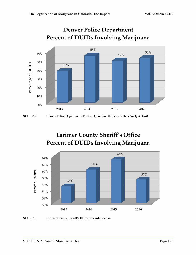
SOURCE: Denver Police Department, Traffic Operations Bureau via Data Analysis Unit
SOURCE: Larimer County Sheriff’s Office, Records Section
0%
10%
20%
30%
40%
50%
60%
2013 2014 2015 2016
37%
55%
49%52%
Per
cen
tag
e o
f D
UID
sDenver Police Department
Percent of DUIDs Involving Marijuana
50%
52%
54%
56%
58%
60%
62%
64%
2013 2014 2015 2016
55%
60%
63%
57%
Per
cen
t P
osi
tiv
e
Larimer County Sheriff's Office
Percent of DUIDs Involving Marijuana

The Legalization of Marijuana in Colorado: The Impact Vol. 5/October 2017
SECTION 2: Youth Marijuana Use Page | 27
SOURCE: Colorado Department of Transportation (CDOT)
Per CDOT, the total number of traffic accidents in Colorado for 2016 was not
available at the time of this report’s publication.
NOTE: ROCKY MOUNTAIN HIDTA HAS BEEN ASKED ABOUT THE TOTAL NUMBER OF
TRAFFIC ACCIDENTS SEEN IN COLORADO SINCE LEGALIZATION AND IS,
THEREFORE, PROVIDING THE DATA. ROCKY MOUNTAIN HIDTA IS NOT
EQUATING ALL TRAFFIC ACCIDENTS WITH MARIJUANA LEGALIZATION.
Related Costs
Economic Cost of Vehicle Accidents Resulting in Fatalities: According to the National
Highway Traffic Safety Administration report, The Economic and Societal Impact of Motor
Vehicles Crashes, 2010, the total economic costs for a vehicle fatality is $1,398,916. That
includes property damage, medical, insurance, productivity, among other
considerations. 2
Cost of Driving Under the Influence: The cost associated with the first driving-under-
the-influence (DUI) offense is estimated at $10,270. Costs associated with a DUID
(driving-under-the-influence-of-drugs) are very similar to those of a DUI/alcohol. 3
124,846
117,228
111,899
104,748
101,627
99,011
100,994
100,832
107,604
115,455
120,700
0
20,000
40,000
60,000
80,000
100,000
120,000
140,000
160,000
2005 2006 2007 2008 2009 2010 2011 2012 2013 2014 2015
Nu
mb
er o
f A
ccid
ents
Total Number of Traffic Accidents
in Colorado

The Legalization of Marijuana in Colorado: The Impact Vol. 5/October 2017
SECTION 2: Youth Marijuana Use Page | 28
Case Examples
Traffic Fatalities Linked to Marijuana are up Sharply in Colorado: Since the
legalization of recreational marijuana, the number of fatal accidents involving drivers
who tested positive for marijuana has “increased at a quicker rate than the increase of
pot usage in Colorado since 2013.” Many family members and loved ones of victims
involved in these fatal accidents are speaking out about the inability for authorities to
properly test for impairment.
“‘I never understood how we’d pass a law without first understanding
the impact better,’ said Barbara Deckert, whose fiancée, Ron Edwards,
was killed in 2015 in a collision with a driver who tested positive for
marijuana use below the legal limit and charged only with careless
driving. ‘How do we let that happen without having our ducks in a
row? And people are dying.’”
On January 13, 2016 just past 2 a.m., “Cody Gray, 19, and his running
buddy, Jordan Aerts, 18, were joyriding around north Denver in a car
they had stolen a few hours earlier. Ripping south along Franklin
Street, where it curves hard to the right onto National Western Drive,
Gray lost control, drove through a fence and went straight onto the
bordering railroad tracks. The car rolled and Gray was ejected. Both
died.” Corina Triffet, mother of Cody Gray, did not know that an
autopsy done revealed that her son had 10ng/mL , twice the legal limit,
of THC in his system when he died, until the Denver Post contacted
her. “There’s just no limit on what they can take, whether it’s smoking
it or edibles,” said Triffet and “I just can’t imagine people are getting
out there to drive when they’re on it. But my son apparently did, and
there it is.”
Too little is understood about how marijuana impairs a person’s ability to operate a
vehicle. Due to this lack of understanding the Denver Post stated, “Even coroners who
occasionally test for the drug bicker over whether to include pot on a driver’s death
certificate.”
“’No one’s really sure of the broad impact because not all the drivers are
tested, yet people are dying,’ said Montrose County Coroner Dr. Thomas
Canfield. ‘It’s this false science that marijuana is harmless, … but it’s not,
particularly when you know what it does to your time and depth perception,
and the ability to understand and be attentive to what’s around you.’”

The Legalization of Marijuana in Colorado: The Impact Vol. 5/October 2017
SECTION 2: Youth Marijuana Use Page | 29
Colorado now mandates that traffic fatalities within the state be analyzed to see
what role drugs played in the crashes. State police are re-analyzing samples from
suspected drunk drivers in 2015 and a Denver Post source stated, “more than three in
five also tested positive for active THC.” However, testing remains expensive and most
departments will stop testing when a driver tests positive for alcohol impairment. 1
20-Year-Old Colorado Man Kills 8-Year-Old Girl While Driving High: A former star
athlete at Mead High School accused of fatally running over an 8-year-old Longmont
girl on her bike told police he thought he'd hit the curb — until he saw the girl's
stepfather waving at him, according to an arrest affidavit released July 29, 2016.
Kyle Kenneth Couch, 20, turned right on a red light at the same time Peyton
Knowlton rolled into the crosswalk on May 20, 2016. The girl was crushed by the rear
right tire of the Ford F-250 pickup, and died from her injuries. Couch, of Longmont,
surrendered to police Friday on an arrest warrant that included charges of vehicular
homicide and driving under the influence of drugs. One blood sample collected more
than two hours after the collision tested positive for cannabinoids, finding 1.5
nanograms of THC per milliliter of blood. That's below Colorado's legal limit of 5
nanograms per milliliter. But Deputy Police Chief Jeff Satur said the law allows the
DUI charge when those test results are combined with officer observations of impaired
behavior and marijuana evidence found inside Couch's pickup.
The presumptive sentencing range for vehicular homicide, a Class 3 felony, is four to
12 years in prison.
Couch attends Colorado Mesa University where, in 2015, he appeared in six games
as a linebacker as a red shirt freshman for the football team. In 2013, Couch became the
first athlete from Mead High School to win a state title when he captured the Class 4A
wrestling championship at 182 pounds. He was named the Times-Call's Wrestler of the
Year that season and was able to defend his crown a year later, winning the 4A title at
195 pounds to cap his senior season with a 49-1 record.
Couch, now 20, has been arrested on suspicion of vehicular homicide and driving
under the influence of marijuana in connection with the death of 8-year-old Peyton
Knowlton. 4
Valedictorian and Friends Die in Fatal Crash after Using Marijuana: An 18 year old
recent valedictorian of St. John’s Military School, Jacob Whitting, was driving his truck
with his friends when he “lost control and ran off the road, rolling down an
embankment and into a creek.” Whitting, along with 2 of the 3 other passengers, ages 16
and 19, died in the crash. According to the toxicology report, all three deceased
teenagers had taken Xanax and marijuana. Whitting’s toxicology “recorded THC levels
at higher than 5 nanograms or more of active THC (delta-9 tetrahydrocannabinol) per
milliliter of blood, which under Colorado law is considered impaired while driving.” 5

The Legalization of Marijuana in Colorado: The Impact Vol. 5/October 2017
SECTION 2: Youth Marijuana Use Page | 30
Man Killed, Woman and Two Children Injured after Vehicle Careens off I-76:
Anthony Griego, 28, “was driving very aggressively and speeding, and had been trying
to pass a semi-truck using the shoulder when he lost control,” according to Colorado
State Patrol, just before 7 a.m. on December 27, 2016. “Troopers say Griego lost control,
blew thought a guardrail, went airborne and flipped the truck nearly 20 feet down onto
the road below.” Both Griego and the adult female passenger were not wearing
seatbelts and were ejected from the vehicle. Griego died at the scene. The female
passenger suffered a shattered pelvis, broke her spine in three places, and was in a
coma. The two children passengers, 7 year-old Jazlynn, had a punctured lung and, 6
year-old Alexis, had a fractured skull and broken collar bone. An autopsy of Griego
showed he had 19ng/mL of THC in his system at the time of the crash. That is nearly 4
times the legal limit. 6, 7
“I fell asleep” Boulder Teen Pleads Guilty to Vehicular Homicide: Quinn Hefferan
faces up to two years in the Colorado Department of Youth Corrections for killing Stacy
Reynolds (30) and Joe Ramas (39) on May 7th 2016. Hefferan, who was 17 years old at
the time of the accident, told the judge he “had split a joint with his friends” and fell
asleep at the wheel while trying to make his midnight curfew. Hefferan rear ended the
couple “at speeds upwards of 45 miles per hour... police did not find any evidence the
teen driver tried to brake before the crash.” According to the toxicology report, he had 4
times the legal limit of THC in his system. Cassie Drew, a friend of the couple says,
“It’s not about resentment or getting back, or feeling angry. [Hefferan’s] life is forever
changed and we recognize that, we recognize how much this will impact him and his
family.” 8, 9
Middle School Counselor Killed by High Driver as She Helped Fellow Motorist:
On July 10, 2016, a counselor at Wolf Point Middle School, in Montana, was hit by a car
and killed by an impaired driver in Colorado as she stopped to help another driver.
The Jefferson County coroner in Colorado identified the woman as Jana Elliott, 56. She
died of multiple blunt force trauma injuries. Elliott is identified as a counselor for the
sixth grade in Montana.
The driver who hit Elliott, identified as Curtis Blodgett, 24, is being charged with
vehicular homicide for allegedly smoking marijuana prior to the crash, according to The
Denver Post. Blodgett allegedly admitted he had smoked marijuana that day.
Detectives are working to determine whether Blodgett was legally impaired at the time
of the crash. “How much he had in his system and what he had in his system will
determine whether additional charges could be filed,” Lakewood Police Spokesman
Steve Davis told The Post (subsequent testing revealed Blodgett had 4.8 ng/mL of THC
in his system).

The Legalization of Marijuana in Colorado: The Impact Vol. 5/October 2017
SECTION 2: Youth Marijuana Use Page | 31
According to the Lakewood Police Department Traffic Unit, Elliott was driving on
US Highway 6 when a vehicle traveling in the left lane lost the bicycle it was carrying
on its top. The driver of the vehicle stopped to retrieve the bike and Elliott stopped
along the shoulder as well to help. After they retrieved the bicycle and were preparing
to drive away, another vehicle rear ended Elliott’s vehicle at a speed of 65 mph. Elliott
was killed in the crash. 10
Suspected DUI Driver Runs A Red Light: On August 30th, 2017, at around 5:30 a.m. a
driver in a Toyota 4Runner ran a red light and crashed into a public transit bus. Two
people were injured in the crash. Police investigating the crash found “marijuana in the
4Runner and the crash is being investigated as a possible DUI for alcohol and
marijuana.” The typically busy intersection in Wheat Ridge, CO had to be closed down
for several hours during rush hour. 11
For Further Information on Impaired Driving See Page 147
Sources
1 David Migoya, “Exclusive: Traffic fatalities linked to marijuana are up sharply
in Colorado. Is legalization to blame?” The Denver Post, August 25th, 2017,
<http://www.denverpost.com/2017/08/25/colorado-marijuana-traffic-fatalities/>,
accessed August 25th, 2017.
2 National Center for Statistics and Analysis, “The Economic and Societal Impact
Of Motor Vehicle Crashes,” National Highway Traffic Safety Administration,
Washington, DC, revised May 2015,
<https://crashstats.nhtsa.dot.gov/Api/Public/ViewPublication/812013>, accessed August
31st, 2017.
3 Cost of a DUI brochure,
<https://www.codot.gov/library/brochures/COSTDUI09.pdf/view>, accessed February
19, 2015.

The Legalization of Marijuana in Colorado: The Impact Vol. 5/October 2017
SECTION 2: Youth Marijuana Use Page | 32
4 Amelia Arvesen, Times-Call, July 29, 2016, “Driver accused of killing Longmont
girl riding bike thought he’d hit curb,”
<http://www.timescall.com/news/crime/ci_30185142/driver-accused-killing-longmont-
girl-bike-thought-hed,” accessed July 29, 2016.
5 Yesenia Robles, “Autopsy shows teens in fatal Conifer crash had traces of
Xanax and marijuana in their system,” The Denver Post, July 7th 2016,
<http://www.denverpost.com/2016/07/07/teens-conifer-crash-traces-drugs-thc/>,
accessed August 28th, 2017.
6 Allison Sylte, “Man killed, woman and two children injured after vehicle
careens off I-76,” 9NEWS, December 27, 2016, <http://www.9news.com/traffic/man-
killed-woman-and-two-children-injured-after-vehicle-careens-off-i-76/379100251>,
accessed September 25, 2017.
7 Macradee Aegerter, “CSP: Driver who went off elevated section of I-76 may
have been high,” FOX31 Denver, December 28, 2016, <http://kdvr.com/2016/12/28/csp-
marijuana-may-have-been-contributing-factor-in-deadly-crash/>, accessed September
25, 2017.
8 Michell Byars, “’I fell asleep’: Boulder teen pleads guilty to vehicular homicide,
DUI in crash that killed 2,” The Daily Camera, December 16th, 2016,
<http://www.dailycamera.com/news/boulder/ci_30665690/quinn-hefferan-boulder-fatal-
crash-dui>, accessed August 23, 2017.
9 Lauren DiSpirito, “Teen Accused Of Being Stoned In Crash That Killed Boulder
Couple,” CBS Denver, June 11th 2016, <http://Denver.cbslocal.com/2016/06/11/stacey-
reynolds-joe-rama-fatal-crash/>, accessed August 23rd, 2017.
10 Aja Goare, “Wolf Point school counselor killed by car while helping other
driver in Colorado,” KTVS.com, July 13, 2016,
<http://www.ktvq.com/story/32440083/wolf-point-school-counselor-killed-by-car-while-
helping-other-driver-in-colorado>, accessed July 13, 2016.
11 Chuck Hickey, “Police: Suspected DUI driver runs red light, crashed
into RTD bus in Wheat Ridge,” Fox 31 Denver, August 30th 2017,
<http://kdvr.com/2017/08/30/rtd-bus-3-vehicles-involved-in-wheat-ridge-crash/>,
accessed August 30th, 2017.

The Legalization of Marijuana in Colorado: The Impact Vol. 5/October 2017
SECTION 2: Youth Marijuana Use Page | 33
SECTION 2: Youth Marijuana
Use
Some Findings
Youth past month marijuana use increased 12 percent in the three-year average
(2013-2015) since Colorado legalized recreational marijuana compared to the
three-year average prior to legalization (2010-2012).
The latest 2014/2015 results show Colorado youth ranked #1 in the nation for past
month marijuana use, up from #4 in 2011/2012 and #14 in 2005/2006.
Colorado youth past month marijuana use for 2014/2015 was 55 percent higher
than the national average compared to 39 percent higher in 2011/2012.
The top ten states with the highest rate of current marijuana youth use were all
medical marijuana states, whereas the bottom ten were all non-medical-
marijuana states.
Surveys NOT Utilized
Rocky Mountain HIDTA did not use the following datasets in this report
because of the following reasons:
Healthy Kids Colorado Survey (HKCS)
The HKCS shows a 7.6 percent increase in student marijuana use from 2013 (19.7
percent) to 2015 (21.2 percent). According to a front page article in The Denver Post
(June 21, 2016), the increase was not statistically significant and thus “Pot use among
Colorado teens flat.” In fact, The Denver Post released an editorial on June 22, 2016 titled
“Colorado’s good news on teen pot use.” An analysis of the data paints a different
picture of student marijuana use in Colorado.

The Legalization of Marijuana in Colorado: The Impact Vol. 5/October 2017
SECTION 2: Youth Marijuana Use Page | 34
Some concerns with the HKCS include:
Jefferson County (the 2nd largest school district), Douglas County (the 3rd largest
school district), El Paso County (Colorado Springs, 2nd largest metro area), and
Weld County results were listed as N/A which means data not available due to
low participation in the region.
NOTE: This is a similar reason why HKCS results were considered unweighted by
the national YRBS survey.
In 2015 the HKCS survey had a response rate of 46 percent, which is well below
the 60 percent rate required by YRBS. Even though HKCS samples a large
number of students, their participation rate is below the industry standard for
weighted data.
From 2013 to 2015, marijuana use:
o High School – increased 14 percent among seniors and 19 percent among
juniors.
o Middle School – increased 96 percent for 7th Graders and 144 percent
among 6th Graders.
SOURCE: Colorado Department Public Health and Environment, Healthy Kids Colorado Survey
For a detailed analysis and additional data, go to www.rmhidta.org and click on the
Reports tab to read “Colorado Youth Marijuana Use: Up – Down – Flat? Examine the
Data and You Decide!”
0.0
5.0
10.0
15.0
20.0
25.0
30.0
6th 7th 8th 9th 10th 11th 12th
0.9
4.5
8.7
13.7
19.0
22.124.3
2.2
8.8 8.8
12.4
18.8
26.327.8
Per
cen
t o
f P
rev
alen
ce
Healthy Kids Colorado Survey:
Current Marijuana Use for High School and
Middle School Students in Colorado
2013 2015

The Legalization of Marijuana in Colorado: The Impact Vol. 5/October 2017
SECTION 2: Youth Marijuana Use Page | 35
Monitoring the Future (MTF) Study
Although Colorado cited Monitoring the Future data in a response letter to Attorney
General Jeff Sessions, the study is designed to be nationally-representative and not
state-representative. MTF does not provide usable estimates for the specific state of
Colorado because of the state’s relatively small size. Colorado is only 1.6 percent of the
total U.S. population; thus, the sampling would only be 1.6 percent of Colorado schools
(400) or about 6 schools per year. Since 2010, the survey sampled an average of 4.6
Colorado schools. In 2014 and 2015, there were four schools surveyed each year of
which three were eighth grade. Therefore, the MTF study is not useful for state data
pertaining to Colorado for school-age drug use data and trends.
Centers for Disease Control Youth Risk Behavior Survey (YRBS)
In 2015, Colorado fell short of the required 60 percent participation rate and was,
therefore, not included with weighted data in this survey. Additionally, upon further
review, it was discovered that since 1991 the state of Colorado has only been
represented in the High School YRBS survey with weighted data four times. Since 1995,
Colorado has only been represented in the Middle School YRBS survey by weighted
data twice. States that participated in the 2015 Middle School and High School YRBS
surveys are represented in dark purple in the below maps. It should be noted, in 2015,
high schools in the following ten states were not included with weighted high school
data: Utah, Colorado, Kansas, Texas, Louisiana, Georgia, Iowa, Wisconsin, Ohio, and
New Jersey. Washington, Oregon, and Minnesota did not participate in the survey.
Centers for Disease Control Youth Risk Behavior Survey
2015 YRBS Participation Map
Middle Schools High Schools
SOURCE: Centers for Disease Control and Prevention, Adolescent and School Health, YRBS Participation
Maps and History http://www.cdc.gov/healthyyouth/data/yrbs/participation.htm

The Legalization of Marijuana in Colorado: The Impact Vol. 5/October 2017
SECTION 2: Youth Marijuana Use Page | 36
Use Data
Youth Ages 12 to 17 Years Old
SOURCE: SAMHSA.gov, National Survey on Drug Use and Health 2014 and 2015
SOURCE: SAMHSA.gov, National Survey on Drug Use and Health 2014 and 2015
0.00%
2.00%
4.00%
6.00%
8.00%
10.00%
12.00%
2010-2012
Pre-Recreational Legalization
2013-2015
Post-Recreational Legalization
10.60%
11.85%
Av
erag
e P
erce
nt
Average Past Month Use of Marijuana
Youth Ages 12 to 17 Years Old
12% Increase
6.74 6.67 6.67 7.03 7.38 7.64 7.55 7.15 7.22 7.20
7.608.15
9.1310.17 9.91
10.72 10.4711.16
12.5611.13
0.00
2.00
4.00
6.00
8.00
10.00
12.00
14.00
16.00
05/06 06/07 07/08 08/09 09/10 10/11 11/12 12/13 13/14 14/15
Av
erag
e P
erce
nt
Annual Averages of Data Collection
Past Month Marijuana Use
Youth Ages 12 to 17 Years Old
National Average Colorado Average
Commercialization
Legalization
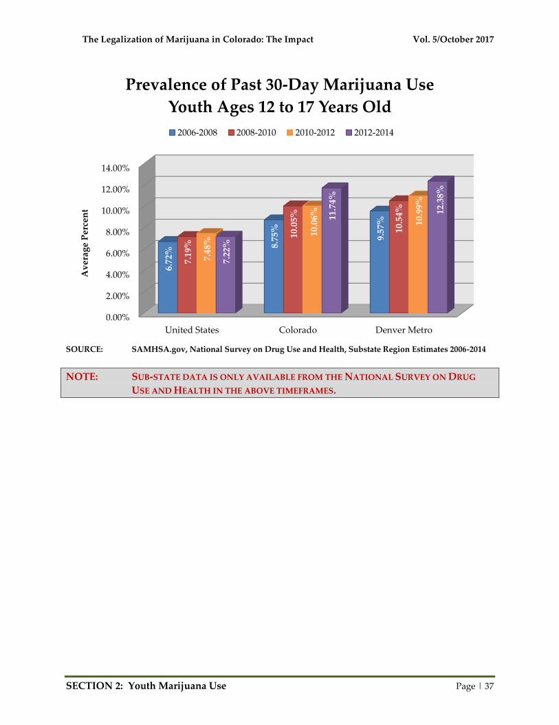
The Legalization of Marijuana in Colorado: The Impact Vol. 5/October 2017
SECTION 2: Youth Marijuana Use Page | 37
SOURCE: SAMHSA.gov, National Survey on Drug Use and Health, Substate Region Estimates 2006-2014
NOTE: SUB-STATE DATA IS ONLY AVAILABLE FROM THE NATIONAL SURVEY ON DRUG
USE AND HEALTH IN THE ABOVE TIMEFRAMES.
0.00%
2.00%
4.00%
6.00%
8.00%
10.00%
12.00%
14.00%
United States Colorado Denver Metro
6.72
%
8.75
%
9.57
%
7.19
%
10.0
5%
10.5
4%
7.48
%
10.0
6%
10.9
9%
7.22
%
11.7
4%
12.3
8%
Av
erag
e P
erce
nt
Prevalence of Past 30-Day Marijuana Use
Youth Ages 12 to 17 Years Old
2006-2008 2008-2010 2010-2012 2012-2014

The Legalization of Marijuana in Colorado: The Impact Vol. 5/October 2017
SECTION 2: Youth Marijuana Use Page | 38
SOURCE: SAMHSA.gov, National Survey on Drug Use and Health 2014 and 2015
NOTE: *California, Massachusetts, Maine and Nevada voted to legalize recreational marijuana in
November 2016
**States that had legislation for medical marijuana signed into effect during 2015
0.00% 2.00% 4.00% 6.00% 8.00% 10.00% 12.00%
Utah
Alabama
Nebraska
Mississippi
Iowa
**Louisiana
Oklahoma
Virginia
Tennessee
North Carolina
**Ohio
West Virginia
Hawaii
**North Dakota
Minnesota
Kentucky
South Dakota
Kansas
**Arkansas
Idaho
Illinois
Missouri
South Carolina
Wyoming
**Florida
New Jersey
Texas
Georgia
**Pennsylvania
*Nevada
Delaware
New York
Wisconsin
Arizona
Michigan
Indiana
*California
Connecticut
New Mexico
Montana
Washington
Maryland
*Massachusetts
Oregon
New Hampshire
*Maine
Rhode Island
Alaska
Vermont
Colorado
Past Month Usage, 12 to 17 Years Old, 2014/2015
As of 2015:
Legalized Recreational/Medical Marijuana
Legalized Medical Marijuana
Non-Legalized Medical Marijuana
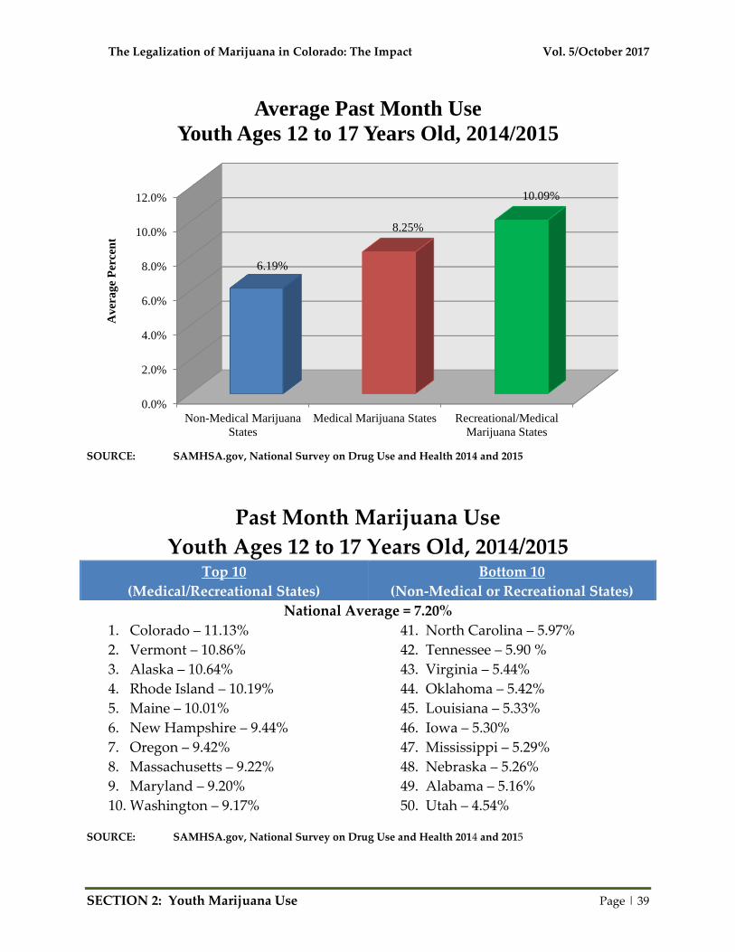
The Legalization of Marijuana in Colorado: The Impact Vol. 5/October 2017
SECTION 2: Youth Marijuana Use Page | 39
SOURCE: SAMHSA.gov, National Survey on Drug Use and Health 2014 and 2015
Past Month Marijuana Use
Youth Ages 12 to 17 Years Old, 2014/2015 Top 10
(Medical/Recreational States)
Bottom 10
(Non-Medical or Recreational States)
National Average = 7.20%
1. Colorado – 11.13% 41. North Carolina – 5.97%
2. Vermont – 10.86% 42. Tennessee – 5.90 %
3. Alaska – 10.64% 43. Virginia – 5.44%
4. Rhode Island – 10.19% 44. Oklahoma – 5.42%
5. Maine – 10.01% 45. Louisiana – 5.33%
6. New Hampshire – 9.44% 46. Iowa – 5.30%
7. Oregon – 9.42% 47. Mississippi – 5.29%
8. Massachusetts – 9.22% 48. Nebraska – 5.26%
9. Maryland – 9.20% 49. Alabama – 5.16%
10. Washington – 9.17% 50. Utah – 4.54%
SOURCE: SAMHSA.gov, National Survey on Drug Use and Health 2014 and 2015
0.0%
2.0%
4.0%
6.0%
8.0%
10.0%
12.0%
Non-Medical Marijuana
States
Medical Marijuana States Recreational/Medical
Marijuana States
6.19%
8.25%
10.09%
Av
era
ge
Per
cen
tAverage Past Month Use
Youth Ages 12 to 17 Years Old, 2014/2015
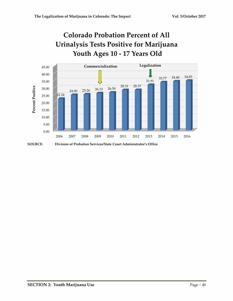
The Legalization of Marijuana in Colorado: The Impact Vol. 5/October 2017
SECTION 2: Youth Marijuana Use Page | 40
SOURCE: Division of Probation Services/State Court Administrator’s Office
0.00
5.00
10.00
15.00
20.00
25.00
30.00
35.00
40.00
45.00
2006 2007 2008 2009 2010 2011 2012 2013 2014 2015 2016
22.2424.90 25.26 26.15 26.59
28.31 28.37
31.9133.77 34.40 34.83
Per
cen
t P
osi
tiv
eColorado Probation Percent of All
Urinalysis Tests Positive for Marijuana
Youth Ages 10 - 17 Years Old
Commercialization Legalization
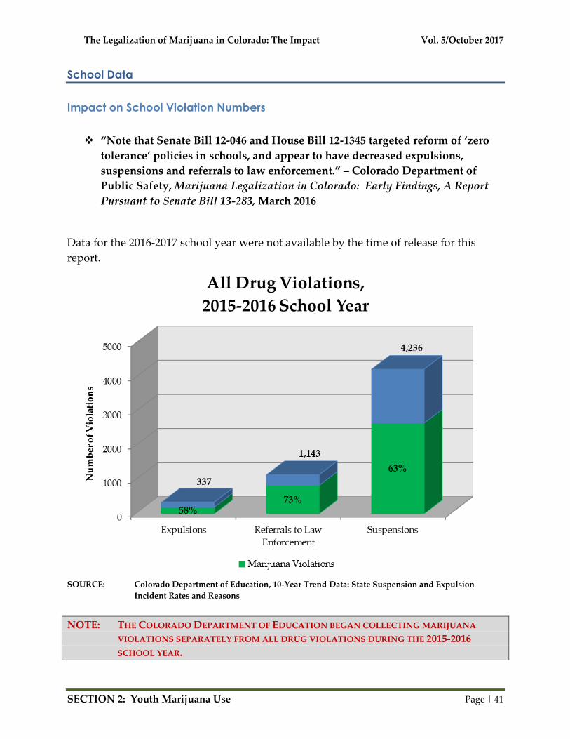
The Legalization of Marijuana in Colorado: The Impact Vol. 5/October 2017
SECTION 2: Youth Marijuana Use Page | 41
School Data
Impact on School Violation Numbers
“Note that Senate Bill 12-046 and House Bill 12-1345 targeted reform of ‘zero
tolerance’ policies in schools, and appear to have decreased expulsions,
suspensions and referrals to law enforcement.” – Colorado Department of
Public Safety, Marijuana Legalization in Colorado: Early Findings, A Report
Pursuant to Senate Bill 13-283, March 2016
Data for the 2016-2017 school year were not available by the time of release for this
report.
SOURCE: Colorado Department of Education, 10-Year Trend Data: State Suspension and Expulsion
Incident Rates and Reasons
NOTE: THE COLORADO DEPARTMENT OF EDUCATION BEGAN COLLECTING MARIJUANA
VIOLATIONS SEPARATELY FROM ALL DRUG VIOLATIONS DURING THE 2015-2016
SCHOOL YEAR.

The Legalization of Marijuana in Colorado: The Impact Vol. 5/October 2017
SECTION 2: Youth Marijuana Use Page | 42
SOURCE: Colorado Department of Education, 10-Year Trend Data: State Suspension and Expulsion
Incident Rates and Reasons
In school year 2015/2016, 62 percent of all drug expulsions and suspensions
were for marijuana violations.
SOURCE: Colorado Department of Education, 10-Year Trend Data: State Suspension and Expulsion
Incident Rates and Reasons
In school year 2015/2016, 73 percent of all drug related referrals to law
enforcement were for marijuana violations.

The Legalization of Marijuana in Colorado: The Impact Vol. 5/October 2017
SECTION 2: Youth Marijuana Use Page | 43
SOURCE: Colorado Department of Education
NOTE: ROCKY MOUNTAIN HIDTA HAS BEEN ASKED ABOUT THE NUMBER OF SCHOOL
DROPOUTS IN COLORADO NUMEROUS TIMES AND IS, THEREFORE, PROVIDING THE
DATA. ROCKY MOUNTAIN HIDTA IS NOT ATTRIBUTING THE NUMBER OF
DROPOUTS TO MARIJUANA LEGALIZATION.
Colorado School Resource Officer Survey
In June 2017, 76 school resource officers (SRO) participated in a survey concerning
marijuana in schools. The majority were assigned to high schools and had a tenure of
three years or more as a SRO. They were asked for their professional opinion on a
number of questions. The questions and their responses are shown in the following
pages.
10,200
10,400
10,600
10,800
11,000
11,200
2012-2013 2013-2014 2014-2015 2015-2016
10,664
10,546
11,114
10,530
Nu
mb
er o
f D
rop
ou
tsNumber of Reported School Dropouts

The Legalization of Marijuana in Colorado: The Impact Vol. 5/October 2017
SECTION 2: Youth Marijuana Use Page | 44
Question: Since the legalization of recreational marijuana, what impact has there
been on marijuana-related incidents at your school?
SOURCE: Colorado Association of School Resource Officers (CASRO) and Rocky Mountain HIDTA
Question: What were the most predominant marijuana violations by students on
campus?
SOURCE: Colorado Association of School Resource Officers (CASRO) and Rocky Mountain HIDTA
86%
4%
10%
Increase
Decrease
No Change
Impact on Marijuana-Related Incidents, 2017
0%
5%
10%
15%
20%
25%
30%
35%
40%
45%
50%
Student sharing
marijuana with
other students
Student selling
marijuana to
other students
Student in
possession of
marijuana
infused edibles
Student in
possession of
marijuana
Student under
the influence
during school
hours
2%5% 6%
36%
44%
Per
cen
t o
f S
RO
Res
po
nse
s
Predominant Marijuana Violations, 2017

The Legalization of Marijuana in Colorado: The Impact Vol. 5/October 2017
SECTION 2: Youth Marijuana Use Page | 45
Question: Where do the students get their marijuana?
SOURCE: Colorado Association of School Resource Officers (CASRO) and Rocky Mountain HIDTA
School Counselor Survey
Since the 2015 survey, the Colorado School Counselor Association has elected
not to participate in any further surveys.
In August 2015, 188 school counselors participated in a survey concerning the
legalization of marijuana in schools. The majority were assigned to high schools with
an average tenure of ten years. They were asked for their professional opinion on a
number of question. The questions and their responses are shown in the following
pages.
0%
5%
10%
15%
20%
25%
30%
35%
40%
45%
Medical
Marijuana
Cardholders
Medical
Marijuana
Dispensaries
Medical
Marijuana
Caregivers
Parents Black Market Friend Who
Obtained it
Legally
7%5%
2%
23% 26%
39%
Per
cen
t o
f S
RO
Res
po
nse
s
Student Marijuana Source, 2017

The Legalization of Marijuana in Colorado: The Impact Vol. 5/October 2017
SECTION 2: Youth Marijuana Use Page | 46
Question: Since the legalization of recreational marijuana, what impact has there
been on marijuana-related incidents at your school?
SOURCE Colorado School Counselor Association (CSCA) and Rocky Mountain HIDTA
Question: What were the most predominant marijuana violations by students on
campus?
SOURCE Colorado School Counselor Association (CSCA) and Rocky Mountain HIDTA
68%2%
30% Increased
Decreased
No Change
Impact on Marijuana-Related Incidents, 2015
0%
10%
20%
30%
40%
50%
60%
Student selling
marijuana to
other students
Student sharing
marijuana with
other students
Student in
possession of
marijuana
infused edibles
Student in
possession of
marijuana
Student under
the influence
during school
hours
5% 6%
9%
30%
51%
Per
cen
t o
f C
ou
nse
lor
Res
po
nse
s
Predominant Marijuana Violations, 2015

The Legalization of Marijuana in Colorado: The Impact Vol. 5/October 2017
SECTION 2: Youth Marijuana Use Page | 47
Question: Where do the students get their marijuana?
SOURCE Colorado School Counselor Association (CSCA) and Rocky Mountain HIDTA
Case Examples
My son and his Marijuana: “It was February 6th at 3:15 a.m. when my oldest son woke
me and urgently whispered that his brother had just tried to take his own life. I
couldn’t comprehend that my second-born, a high achieving, gifted young man had just
attempted suicide by hanging. Thankfully, his brother discovered him and saved his life
before we lost him. It changed our family forever.
Later that morning after the assessment and intake procedure, the hospital social
worker explained that my son’s prescription for Adderall combined with his heavy
marijuana use had caused a psychotic break called marijuana induced psychosis. She
said this was quite common among young people today. I felt blindsided as I had no
idea my son was using marijuana.
Sadly, in-patient treatment was not successful, nor was out-patient treatment.
Our lives began to revolve around our son’s addiction and the never-ending
appointments, meetings, confrontations, stress, and bizarre drama that we never
Student Marijuana Source, 2015

The Legalization of Marijuana in Colorado: The Impact Vol. 5/October 2017
SECTION 2: Youth Marijuana Use Page | 48
imagined we would experience. It was both frustrating and heartbreaking to listen as
my son frequently described his passionate commitment to marijuana and observe his
inability to see how negatively it impacted – even controlled him.
We learned we were not fighting a behavior but a mind-set that was cemented
into his belief system. Marijuana had become his life, his religion, and his identity. In
spite of a multitude of problems and ongoing depression that continue to prevent him
from living successfully, his belief that marijuana will solve all of his troubles remains
ingrained in him and leaves our family feeling fearful and often hopeless to help him.” 1
Teen Shot While Trying to Sell Marijuana: While attempting to sell marijuana to a car
filled with four other teenagers, an 18 year old in Greeley, Colorado was shot with a
handgun. The seller had been leaning into the car window when the occupants shot
him and quickly drove away. The wound sustained by the teenager was not life
threatening. 2
One Teen Wounded, Another Killed While Trying to Steal Marijuana: Shortly after 2
a.m. on Sunday, October 9th, 2016, Denver Police received a call from a 14-year-old boy
stating that he and his friend had been shot. Both boys had been trying to steal
marijuana plants from a backyard when the resident was alerted to their presence and
fired multiple shots at the boys. Both boys were struck as they were trying to escape the
backyard, the 14-year-old was wounded and the 15-year old boy was killed. The home
owner was arrested and held for investigation of murder, attempted murder and
investigation of felony marijuana cultivation. 3

The Legalization of Marijuana in Colorado: The Impact Vol. 5/October 2017
SECTION 2: Youth Marijuana Use Page | 49
Some Comments from School Resource Officers
They End Up Sick:
o “A student came to after-prom after eating some marijuana edibles. She
later got very sick and was transported by ambulance to the hospital. She
later admitted to being given the edibles by another student.”
o “A student asked another to get them marijuana. Student brought some
edibles, later that week, and then the other student shared the edibles with
5 other people, who became sick. All students were disciplined. It is very
common for students to bring edibles and share with others, and they end
up sick from eating too much.”
o “8th grader brought marijuana brownies to school, gave them to friends
and then overdosed on them and ended up in the hospital.”
Organized and Well-planned Distribution:
o “Students sometimes put Marijuana in Cheetos bags and sell to each
other.”
o “Our agency just processed a 12 year old student for distribution of MJ.
The child admitted to stealing ‘unnoticeable’ amounts of MJ from several
different relatives, who purchased the recreational MJ legally, then sold it
to other students. The 12 year old suspect had also recruited other
students to sell the MJ. The crime was eventually reported by the sister of
one of the accomplices.”
o “Student, age 16 (10th grade) recently came with father from California
(father wanted to start a grow operation) frequently peddled marijuana on
and around campus. Eventually, school/police alerted that he was
packing a gun.”
o “Student has a medicinal marijuana card, became marijuana dealer to
fellow students, arrested and is being prosecuted for distribution.”
o “A student baked THC brownies and sold them at school (10-12 grades).
Students were charged [with distribution] of marijuana, it was organized
and well-planned in school distribution (9-11 grades).
Burglarized Dispensary: “Five male students were found on school grounds with an
overabundance of dabs and shatter that was still in the packaging from a dispensary
that had been burglarized the previous weekend by five masked individuals that were
caught on surveillance tape.”

The Legalization of Marijuana in Colorado: The Impact Vol. 5/October 2017
SECTION 2: Youth Marijuana Use Page | 50
Student Commits Suicide: “Sophomore caught selling marijuana to students on
campus. He was distributing for another student. That student was obtaining high
quality marijuana on the black market. Original was charged and committed suicide 3
days later. Other subject made suicidal statements and received treatment.”
Fine for Their Kids to Use: “Multiple students at my ‘affluent’ middle school obtain
marijuana and use marijuana with their families who all seem to have their own
marijuana grows. Most of these parents think their ‘medicine’ is fine for their kids to
use.”
Social Media Delivery Service: “Students using social media to order up their
hash/marijuana/shatter and have it delivered to their local park or fast food joint. No
names exchanged and very difficult to prove a case. Was able to get a warrant on a
suspect with the help of MED (Marijuana Enforcement Division). “
Attempting to Official a Game: “Referee in possession and smelling like marijuana
while attempting to official a game.”
Leave Campus and Come Back High:
“Students will leave campus and smoke either in their home, parks, or cars
and come back after lunch. Adult dealers have trolled [the] parking lot for
students looking to buy marijuana. Lots of marijuana use at juvenile parties
on the weekend.”
“Most of our marijuana offenses in the schools are at the middle school and
high school level where students leave campus, get high and come back to
school. Some are caught with possession of marijuana and some are only
consuming.”
Young Students Stealing from Parents:
“Ten year old in possession and consuming in school using parents pot and
pipe”
“6th grader stealing and then bringing mom’s medical marijuana to school,
sharing with friends and smoking in bathrooms before school.”
“5th grader stealing recreational marijuana from parents and bringing it to
school, showing it to all his friends and then smoking it at school.”

The Legalization of Marijuana in Colorado: The Impact Vol. 5/October 2017
SECTION 2: Youth Marijuana Use Page | 51
Some Comments from School Counselors
Halls Reek of Pot After Lunch:
“Many kids come back from lunch highly intoxicated from marijuana use. Halls
reek of pot, so many kids are high that it is impossible to apprehend all but the
most impaired.”
“They go off campus and smoke during lunch with friends. They will run home
with friends during lunch and smoke then.”
“There have been several instances of students in their cars on lunch or during
their off hours ‘hotboxing’ or smoking marijuana. Most students are seniors but
on occasion, seniors will provide marijuana to 9th or 10th grade students.”
“2014/2015 school year, several students caught coming back from off-campus
lunch under the influence of marijuana.”
“Had a student come back from lunch, teacher believed that they were high.
Student was escorted to the office, student admitted they were indeed high to the
administrator.”
“Students are often referred after lunch (open campus) after they have been
riding around smoking marijuana with their friends.”
“More and more students are coming back to school high after lunch.”
“In April 2015, students were going out for a break. 2-3 students smoked
marijuana about a block away from school. They smelled like pot when they got
back.”
Just a Plant: “In March of 2015 a fifth grade boy offered marijuana to another fifth
grader on the playground. In October of 2014 a kindergarten girl described the pipe in
her grandmother’s car and the store where you go to buy pipes. In May of 2015 a first
grade girl reported that her mom smokes weed in the garage. ‘It’s not a drug, it’s just a
plant.’”
Arrives at School Stoned:
“At the beginning of the second semester, three middle school boys were
routinely arriving late at school, and noticeable intoxicated.”
“We have middle school students who either come to school high, or have it on
them in a bag. Or they have pipes on them.”
“In May 2015, a teacher witnessed 2 seniors smoking marijuana while driving to
school. One student admitted to having done so; the other denied it.”
“Teaching a lesson in class during first period that started 7:30 AM and 2
students were already high in class.”

The Legalization of Marijuana in Colorado: The Impact Vol. 5/October 2017
SECTION 2: Youth Marijuana Use Page | 52
“A male 13 y/o student fell asleep in several classes. He was interviewed by the
school counselor and the RSO (sic). He was assessed as being high and admitted
that he uses marijuana often before school. He steals it from his older brother.”
“12 yr. old, sixth grader, was suspected of coming to summer school high. When
confronted he told the teacher that he smoked it at home the night before but
denied being high at the time. Later, he confirmed that he had smoked early that
morning. The marijuana came from his mother’s stash.”
New Use of Bathrooms:
“2 students were smoking marijuana in the restroom last year.”
“8th grade male student had marijuana in his locker, classmates reported it. 8th
grade female student smoked a joint in a school bathroom during school hours.
Shared it with a friend.”
“7th grade girl last year had hidden marijuana and a pipe in the girl’s restroom
and told several friends who began getting bathroom break passes from various
classrooms. Security noted an increased traffic flow to and from that restroom
and found the weed and soon after the violators.”
It’s Legal:
“3 or 4 times in the last school year, students have come to school under the
influence after meeting at homes where parents were absent, sharing marijuana
off campus and then bringing it on campus. 7th and 8th grade students have been
involved, and most often their reaction when caught is ‘it’s legal’.”
“I met with at least 5 students last year alone that have been showing significant
signs of drug use or were caught and they all said they will not stop using weed
on a daily basis. Their justification was it’s fine because it’s legal. If it’s legal it’s
not as bad as what adults say about the risks.”
Grades Decline: “I would like to say that in general our Marijuana incidents have not
gone up. We have a savvy population that knows to keep it away from school.
However, I have seen a huge spike in talking with kids about it in my sessions. Last
year I had two very intelligent students (above 4.0) that used marijuana 2-6 times a
week. Both of them had grades decline and significant social emotional issues spike in
the spring of their Senior Year. They also both had violations at school.”
Dad Allows Pot Smoking: “We had reports of two students (brothers) appear to be
high at school. Our officer assessed both of them and discovered that their father, who
had a medical marijuana card, was having them both “smoke a bowl” before school.
He thought it would make their school day easier.”

The Legalization of Marijuana in Colorado: The Impact Vol. 5/October 2017
SECTION 2: Youth Marijuana Use Page | 53
Parents High: “At our elementary school, we have noticed an increased number of
parents showing up to school high. Kids have also brought [marijuana] to school to
show their friends.”
Difficulty in Assessment: “For school personnel, it is more difficult to evaluate what
substance a student is under the influence of. We can smell alcohol and smoked
marijuana but the edibles and vapes are hard to detect.”
Drug Canine Use: “I would like to just offer that we need policy that allows for more
use of drug dogs and not having to forewarn students or parents when these dogs will
be present. Students and especially dealers, the ones we need to catch, are very vigilant
in making adjustments when these resources are used.”
For Further Information on Youth Marijuana Use See Page 151
Sources
1 Jo McGuire, “One Mom’s Story: Marijuana and My Kid,” Jo McGuire Inc., August
29th, 2017, < https://jomcguire.wordpress.com/>, accessed August 29th, 2017.
2 Nate Miller, “Sheriff’s office seeks public’s help to learn more about northeast
Greeley shooting,” The Tribune, May 16, 2017,
<http://www.greeleytribune.com/news/crime/sheriffs-office-seeks-publics-help-to-learn-
more-about-northeast-greeley-shooting/>, accessed September 12, 2017.
3 Kirk Mitchell, “Denver man arrested after allegedly shooting, killing teen in
marijuana-filled backyard,” Denver Post, October 10, 2016,
<http://www.denverpost.com/2016/10/10/marijuana-grow-house-slaying-denver-man-
arrested/>, accessed September 12, 2017.

The Legalization of Marijuana in Colorado: The Impact Vol. 5/October 2017
SECTION 2: Youth Marijuana Use Page | 54
THIS PAGE INTENTIONALLY LEFT BLANK

The Legalization of Marijuana in Colorado: The Impact Vol. 5/October 2017
SECTION 3: Adult Marijuana Use Page | 55
SECTION 3: Adult Marijuana
Use
Some Findings
College age past month marijuana use increased 16 percent in the three-year
average (2013-2015) since Colorado legalized recreational marijuana compared to
the three-year average prior to legalization (2010-2012).
The latest 2014/2015 results show Colorado college-age adults ranked #2 in the
nation for past-month marijuana use, up from #3 in 2011/2012 and #8 in
2005/2006.
Colorado college age past month marijuana use for 2014/2015 was 61 percent
higher than the national average compared to 42 percent higher in 2011/2012.
Adult past-month marijuana use increased 71 percent in the three-year average
(2013-2015) since Colorado legalized recreational marijuana compared to the
three-year average prior to legalization (2010-2012).
The latest 2014/2015 results show Colorado adults ranked #1 in the nation for
past month marijuana use, up from #7 in 2011/2012 and #8 in 2005/2006.
Colorado adult past month marijuana use for 2014/2015 was 124 percent higher
than the national average compared to 51 percent higher in 2011/2012.

The Legalization of Marijuana in Colorado: The Impact Vol. 5/October 2017
SECTION 3: Adult Marijuana Use Page | 56
Use Data
College Age 18 to 25 Years Old
SOURCE: SAMHSA.gov, National Survey on Drug Use and Health 2014 and 2015
SOURCE: SAMHSA.gov, National Survey on Drug Use and Health 2014 and 2015
0.00%
10.00%
20.00%
30.00%
40.00%
2010-2012
Pre-Recreational Legalization
2013-2015
Post-Recreational Legalization
27.04%
31.50%
Av
era
ge
Per
cen
t
Average Past Month Use of Marijuana
College Age 18 to 25 Years Old
16% Increase
16.42 16.34 16.45 17.42 18.39 18.78 18.89 18.91 19.32 19.7
21.43 22.21 23.44 24.2826.35 27.26 26.81
29.0531.24 31.75
0
5
10
15
20
25
30
35
40
45
50
05/06 06/07 07/08 08/09 09/10 10/11 11/12 12/13 13/14 14/15
Av
era
ge
Per
cen
t
Annual Averages of Data Collection
Past Month Marijuana Use
College Age 18 to 25 Years Old
National Average Colorado Average
LegalizationCommercialization

The Legalization of Marijuana in Colorado: The Impact Vol. 5/October 2017
SECTION 3: Adult Marijuana Use Page | 57
SOURCE: SAMHSA.gov, National Survey on Drug Use and Health, Substate Region Estimates 2006-2014
NOTE: SUB-STATE DATA IS ONLY AVAILABLE FROM THE NATIONAL SURVEY ON DRUG
USE AND HEALTH IN THE ABOVE TIMEFRAMES.
0.00%
5.00%
10.00%
15.00%
20.00%
25.00%
30.00%
35.00%
United States Colorado Denver Metro
16
.42
% 21
.87
%
24
.38
%
17
.71
%
25
.38
%
26
.12
%
18
.71
%
27
.22
%
30
.88
%
19
.13
%
29
.86
%
31
.98
%
Av
era
ge
Per
cen
t
Prevalence of Past 30-Day Marijuana Use
College Age 18 to 25 Years Old
2006-2008 2008-2010 2010-2012 2012-2014

The Legalization of Marijuana in Colorado: The Impact Vol. 5/October 2017
SECTION 3: Adult Marijuana Use Page | 58
SOURCE: SAMHSA.gov, National Survey on Drug Use and Health 2013 and 2014
NOTE: *California, Massachusetts, Maine and Nevada voted to legalize recreational marijuana in
November 2016
**States that had legislation for medical marijuana signed into effect during 2015
0.00% 5.00% 10.00% 15.00% 20.00% 25.00% 30.00% 35.00% 40.00%
Utah
Iowa
Idaho
Mississippi
Alabama
**North Dakota
Oklahoma
Texas
Wyoming
Kansas
Tennessee
Hawaii
**Louisiana
Kentucky
Nebraska
**Arkansas
South Dakota
*Nevada
Wisconsin
Virginia
Georgia
West Virginia
Arizona
New Jersey
**Pennsylvania
North Carolina
Minnesota
Missouri
**Ohio
Illinois
*California
New Mexico
Indiana
**Florida
South Carolina
Delaware
Washington
New York
Michigan
Montana
Maryland
Connecticut
Alaska
Oregon
*Massachusetts
Rhode Island
New Hampshire
*Maine
Colorado
Vermont
As of 2015:
Legalized Recreational/Medical Marijuana
Legalized Medical Marijuana
Non-Legalized Medical Marijuana
Past Month Usage, 18 to 25 Years Old, 2014/2015

The Legalization of Marijuana in Colorado: The Impact Vol. 5/October 2017
SECTION 3: Adult Marijuana Use Page | 59
SOURCE: SAMHSA.gov, National Survey on Drug Use and Health 2014 and 2015
Past Month Marijuana Use
College Age 18 to 25 Years Old, 2014/2015
Top 10
(Medical/Recreational States)
Bottom 10
(Non-Medical or Recreational States)
National Average = 19.99%
1. Vermont – 34.95% 41. Kansas – 15.73%
2. Colorado – 31.75% 42. Wyoming – 15.64%
3. Maine – 29.72% 43. Texas – 15.08%
4. New Hampshire – 29.12% 44. Oklahoma – 14.87 %
5. Rhode Island – 28.89% 45. North Dakota – 14.77%
6. Massachusetts – 27.39% 46. Alabama – 14.33%
7. Oregon – 26.29% 47. Mississippi – 13.91%
8. Alaska – 25.02% 48. Idaho – 13.69%
9. Connecticut – 24.99% 49. Iowa – 12.67%
10. Maryland – 24.87% 50. Utah – 11.07%
SOURCE: SAMHSA.gov, National Survey on Drug Use and Health 2014 and 2015
0.00%
5.00%
10.00%
15.00%
20.00%
25.00%
30.00%
Non-Medical
Marijuana States
Medical Marijuana
States
Recreational/Medical
Marijuana States
16.81%
23.19%26.23%
Av
erag
e P
erce
nt
Average Past Month Use
College Age 18 to 25 Years Old, 2014/2015

The Legalization of Marijuana in Colorado: The Impact Vol. 5/October 2017
SECTION 3: Adult Marijuana Use Page | 60
Adults Age 26+ Years Old
SOURCE: SAMHSA.gov, National Survey on Drug Use and Health 2014 and 2015
SOURCE: SAMHSA.gov, National Survey on Drug Use and Health 2014 and 2015
0.00%
2.00%
4.00%
6.00%
8.00%
10.00%
12.00%
14.00%
2010-2012
Pre-Recreational Legalization
2013-2015
Post-Recreational Legalization
7.91%
13.55%
Av
era
ge
Per
cen
t
Average Past Month Use of Marijuana
Adults Ages 26+ Years Old
71% Increase
4.1 4.02 4.06 4.42 4.68 4.8 5.05 5.456.11 6.55
5.32 5.886.88 7.31
8.868.19 7.63
10.13
12.45
14.65
0.00
2.00
4.00
6.00
8.00
10.00
12.00
14.00
16.00
18.00
20.00
05/06 06/07 07/08 08/09 09/10 10/11 11/12 12/13 13/14 14/15
Av
era
ge
Per
cen
t
Annual Averages of Data Collection
Past Month Marijuana Use
Adults Age 26+ Years Old
National Average Colorado Average
Legalization
Commercialization

The Legalization of Marijuana in Colorado: The Impact Vol. 5/October 2017
SECTION 3: Adult Marijuana Use Page | 61
SOURCE: SAMHSA.gov, National Survey on Drug Use and Health, Substate Region Estimates 2006-2014
NOTE: SUB-STATE DATA IS ONLY AVAILABLE FROM THE NATIONAL SURVEY ON DRUG
USE AND HEALTH IN THE ABOVE TIMEFRAMES.
0.00%
2.00%
4.00%
6.00%
8.00%
10.00%
12.00%
14.00%
United States Colorado Denver Metro
4.1
2%
6.2
9%
7.3
3%
4.5
8%
8.9
1%
10
.19
%
4.9
2%
9.2
2% 10
.93
%
5.8
3%
11
.60
%
12
.33
%
Av
era
ge
Per
cen
t
Prevalence of Past 30-Day Marijuana Use
Adults Age 26+ Years Old
2006-2008 2008-2010 2010-2012 2012-2014

The Legalization of Marijuana in Colorado: The Impact Vol. 5/October 2017
SECTION 3: Adult Marijuana Use Page | 62
SOURCE: SAMHSA.gov, National Survey on Drug Use and Health 2014 and 2015
NOTE: *California, Massachusetts, Maine and Nevada voted to legalize recreational marijuana in
November 2016
**States that had legislation for medical marijuana signed into effect during 2015
0.00% 2.00% 4.00% 6.00% 8.00% 10.00% 12.00% 14.00% 16.00%
Iowa
Utah
Mississippi
Alabama
**North Dakota
Texas
Nebraska
Wyoming
**Louisiana
Tennessee
Oklahoma
Virginia
Wisconsin
Idaho
West Virginia
South Dakota
New Jersey
North Carolina
Kentucky
**Arkansas
Kansas
Minnesota
**Ohio
Georgia
**Florida
Delaware
**Pennsylvania
Illinois
South Carolina
Missouri
*Nevada
Indiana
Arizona
Hawaii
Maryland
Connecticut
New York
*California
Michigan
New Mexico
*Massachusetts
Montana
New Hampshire
Washington
Rhode Island
Oregon
Vermont
*Maine
Alaska
Colorado
Past Month Usage, 26+ Years Old, 2014/2015
As of 2015:
Legalized Recreational/Medical Marijuana
Legalized Medical Marijuana
Non-Legalized Medical Marijuana

The Legalization of Marijuana in Colorado: The Impact Vol. 5/October 2017
SECTION 3: Adult Marijuana Use Page | 63
SOURCE: SAMHSA.gov, National Survey on Drug Use and Health 2014 and 2015
Past Month Marijuana Use
Adults Ages 26+ Years Old, 2014/2015
Top 10
(Medical/Recreational States)
Bottom 10
(Non-Medical or Recreational States)
National Average = 6.76%
1. Colorado – 14.65% 41. Tennessee – 4.81%
2. Alaska – 12.83% 42. Louisiana – 4.71%
3. Maine – 11.84% 43. Wyoming – 4.71%
4. Vermont – 11.61% 44. Nebraska – 4.53%
5. Oregon – 10.99% 45. Texas – 4.32%
6. Rhode Island – 10.39% 46. North Dakota – 3.93%
7. Washington – 9.74% 47. Alabama – 3.86%
8. New Hampshire – 9.65% 48. Mississippi – 3.81%
9. Montana – 9.41% 49. Utah – 3.75%
10. Massachusetts – 9.21% 50. Iowa – 3.30%
SOURCE: SAMHSA.gov, National Survey on Drug Use and Health 2014 and 2015
0.00%
2.00%
4.00%
6.00%
8.00%
10.00%
12.00%
14.00%
Non-Medical Marijuana
States
Medical Marijuana States Recreational/Medical
Marijuana States
5.10%
8.01%
12.05%
Av
era
ge
Per
cen
tAverage Past Month Use
Adults Ages 26+ Years Old, 2014/2015
The Legalization of Marijuana in Colorado: The Impact Vol. 5/October 2017
SECTION 3: Adult Marijuana Use Page | 64
Colorado Adult Marijuana Use Demographics1
According to the Colorado Behavior Risk Factor Surveillance System, 2016:
13.6 percent of adults (18+ years old) are current users of marijuana
o Nearly half of current users (47 percent) report using marijuana daily
1 out of 5 current users (20 percent) report driving after using marijuana
Top demographics of those who report current marijuana use:
o Between 18 to 25 years old
Next highest are those 26 to 34 years old
o Black, Non- Hispanic individuals
Next highest are Multiracial (Non-Hispanic) individuals
o Gay/Lesbian/Bisexual adults
o Males
The Southwest region of Colorado reports the highest current marijuana use
o The Southeast and Northwest regions are tied for second highest
NOTE: THE BEHAVIORAL RISK FACTOR SURVEILLANCE SYSTEM (BRFSS) COLLECTS DATA
ON ADULT, INDIVIDUAL-LEVEL BEHAVIORAL HEALTH RISK FACTORS. QUESTIONS
SPECIFICALLY REGARDING MARIJUANA USE WERE NOT ADDED UNTIL 2014.
– MONITORING HEALTH CONCERNS RELATED TO MARIJUANA IN COLORADO: 2016,
COLORADO DEPARTMENT OF PUBLIC HEALTH AND ENVIRONMENT
Case Examples
Young Professional Commits Suicide at 23, Parents Question if THC is to Blame:
Marc Bullard, a young professional with no apparent signs of depression or mental
illness committed suicide in April 2016. He had recently graduated college “near the top
of his college class,” and had been hired at a consulting firm in Denver. “In December of
2015, he was on top of the world explaining in a video documenting his success that,
‘It’s been a good year..’ and that he was looking forward to making plans for 2016.”
After his death, his parents began reading Marc’s personal diaries and found that he
had been writing entries such as:
I found out I was dabbing too much which I already knew and had cut back in February.
But apparently if you overdo it, you can get almost like poison and experience some
negative effects.

The Legalization of Marijuana in Colorado: The Impact Vol. 5/October 2017
SECTION 3: Adult Marijuana Use Page | 65
Marc’s parents began to question “whether his death [was] related to his use of
high potency THC.” Before Marc’s death neither of them had even heard of dabbing.
Marc’s father Mike explained “I had the mindset, well, it’s just marijuana, it’s not going
to hurt anything.” While Marc’s death certificate does not say marijuana was the cause
of death, it “lists a contributing factor to ‘use of concentrated marijuana products.’”2
Parents Charged with Child Abuse for Identical Deaths of Two Babies: In Aurora,
Colorado a couple was booked into jail on two counts of misdemeanor child abuse.
Charges were filed against the couple after their second child died under similar
circumstances as their first child who died two years previously. According to police
reports, both babies “died while sleeping in bed with the parents” and both parents
“appear[ed] to be intoxicated or under the influence.” During the investigation of the
first child’s death there were “indications of alcohol and marijuana use.” The cause of
death as shown on autopsy reports for each child was listed as undetermined, however
per the Arapahoe County Coroner Dr. Kelly Lear-Kaul this is “because suffocation
leaves no trace.” 3
Man Shoots Wife and Kills Neighbor in a “Marijuana and Caffeine-Fueled Paranoid
State”: While home for lunch, Dr. Kenneth Atkinson heard shots being fired next door
at his neighbor’s home. He went outside to see what was going on and “found his
neighbor, Elizabeth Lyons, lying in a driveway, covered in blood.” Elizabeth Lyons had
been shot in the back by her husband Kevin Lyons. Dr. Atkinson attempted to attend to
Mrs. Lyons’ wounds when Kevin Lyons shot at him striking him in the leg. Dr.
Atkinson attempted to call 911 but “more shots rang out as Lyons fired at Atkinson’s
head at point-blank range, fatally wounding him.”
Lyons was sentenced to life in prison plus 352 years in May 2017. Lyons’ public
defender stated in defense of his actions that “Lyons suffered repeated head injuries –
from sports, a car wreck and other activities – that, combined with substance abuse and
difficult circumstances in his life, including marital and financial problems, left him
delusional. Lyons was also in a marijuana and caffeine-fueled paranoid state on the day
of the shooting.” 4
For Further Information on Adult Marijuana Use See Page 152

The Legalization of Marijuana in Colorado: The Impact Vol. 5/October 2017
SECTION 3: Adult Marijuana Use Page | 66
Sources
1 Colorado Behavioral Risk Factor Surveillance System 2016, “Marijuana Use in
Colorado,” Colorado Department of Public Health and Environment.
2 John Ferrugia, “Marijuana in Colorado: A warning about dabbing,” 9News,
<http://www.9news.com/news/health/marijuana-in-colorado-a-warning-about-
dabbing/346018775>, accessed September 12, 2017.
3 Rob Low, March 7, 2017, “Aurora parents charged with child abuse for
identical deaths of 2 babies,” Fox 31News, <http://kdvr.com/2017/03/07/parents-
charged-with-child-abuse-for-identical-deaths-of-2-babies/>, accessed April 19, 2017.
4 Jesse Paul, “Kevin Lyons apologizes for Centennial shooting rampage that
killed beloved doctor, gets life in prison plus 352 years,” Denver Post,
<http://www.denverpost.com/2017/06/05/kevin-lyons-centennial-shooting-rampage-
killed-kenneth-atkinson/>, accessed September 12, 2017.

The Legalization of Marijuana in Colorado: The Impact Vol. 5/October 2017
SECTION 4: Emergency Department and Hospital Marijuana-Related Admissions Page | 67
SECTION 4: Emergency
Department and
Hospital Marijuana-
Related Admissions
Some Findings
The yearly rate of emergency department visits related to marijuana increased 35
percent after the legalization of recreational marijuana (2011-2012 vs. 2013-
September 2015).
Number of hospitalizations related to marijuana:
o 2011 – 6,305
o 2012 – 6,715
o 2013 – 8,272
o 2014 – 11,439
o Jan-Sept 2015 – 10,901
The yearly number of marijuana-related hospitalizations increased 72 percent
after the legalization of recreational marijuana (2009-2012 vs. 2013-September
2015).

The Legalization of Marijuana in Colorado: The Impact Vol. 5/October 2017
SECTION 4: Emergency Department and Hospital Marijuana-Related Admissions Page | 68
Definitions
Marijuana-Related: Also referred to as “marijuana mentions.” Data could be obtained
from lab tests, patient self-admission or some other form of validation obtained by the
provider. Being marijuana-related does not necessarily prove marijuana was the cause
of the emergency department admission or hospitalization.
International Classification of Disease (ICD): A medical coding system used to
classify diseases and related health problems.
**In 2015, ICD-10 (the tenth modification) was implemented in place of
ICD-9. Although ICD-10 will allow for better analysis of disease patterns
and treatment outcomes for the advancement of medical care, comparison
of trends before and after the conversion can be made difficult and/or
impossible. The number of codes increased from approximately 13,600
codes to approximately 69,000 codes. For the above reasons, hospitalization
and emergency department data is only provided pre-conversion to ICD-
10.1
Emergency Department Data
Colorado Department of Public Health and Environment
NOTE: "POSSIBLE MARIJUANA EXPOSURES, DIAGNOSES, OR BILLING CODES IN ANY OF
LISTED DIAGNOSIS CODES: THESE DATA WERE CHOSEN TO REPRESENT THE HD AND
ED VISITS WHERE MARIJUANA COULD BE A CAUSAL, CONTRIBUTING, OR COEXISTING
FACTOR NOTED BY THE PHYSICIAN DURING THE HD OR ED VISIT. FOR THESE DATA,
MARIJUANA USE IS NOT NECESSARILY RELATED TO THE UNDERLYING REASON FOR THE
HD OR ED VISIT. SOMETIMES THESE DATA ARE REFERRED TO AS HD OR ED VISITS
‘WITH ANY MENTION OF MARIJUANA.’” - COLORADO DEPARTMENT OF PUBLIC HEALTH
AND ENVIRONMENT, MONITORING HEALTH CONCERNS RELATED TO MARIJUANA IN
COLORADO: 2014

The Legalization of Marijuana in Colorado: The Impact Vol. 5/October 2017
SECTION 4: Emergency Department and Hospital Marijuana-Related Admissions Page | 69
SOURCE: Colorado Department of Public Health and Environment
NOTE: DATA NOT AVAILABLE PRE-2011. EMERGENCY DEPARTMENT DATA FROM 2011 AND
2012 REFLECTS INCOMPLETE STATEWIDE REPORTING. INFERENCES CONCERNING
TRENDS, INCLUDING 2011 AND 2012, SHOULD NOT BE MADE.
0
200
400
600
800
1,000
(2011-2012)
Pre-Recreational Legalization
(2013-Sept 2015)
Post-Recreational Legalization
660
889 **
Rat
es P
er 1
00,0
00Average Emergency Department Rates
Related to Marijuana*
35% Increase
*Rates of Emergency Department (ED) Visits with Possible Marijuana Exposures, Diagnoses,
or Billing Codes per 100,000 ED Visits by Year in Colorado
**Only 9 months of comparable 2015 data, see ICD definition on page 68
(2013-Sept 2015**)

The Legalization of Marijuana in Colorado: The Impact Vol. 5/October 2017
SECTION 4: Emergency Department and Hospital Marijuana-Related Admissions Page | 70
SOURCE: Colorado Department of Public Health and Environment, Monitoring Health Concerns Related
to Marijuana in Colorado: 2016
NOTE: DATA NOT AVAILABLE PRE-2011. EMERGENCY DEPARTMENT DATA FROM 2011 AND
2012 REFLECTS INCOMPLETE STATEWIDE REPORTING. INFERENCES CONCERNING
TRENDS, INCLUDING 2011 AND 2012, SHOULD NOT BE MADE.
618 701
873
1,039
754 **
0
200
400
600
800
1,000
1,200
2011 2012 2013 2014 Jan - Sept 2015
Rat
es P
er 1
00,0
00Emergency Department Rates
Related to Marijuana*
Legalization
Jan - Sept 2015**
*Rates of Emergency Department (ED) Visits with Possible Marijuana Exposures, Diagnoses, or
Billing Codes per 100,000 ED Visits by Year in Colorado
**Only 9 months of comparable 2015 data, see ICD definition on page 68

The Legalization of Marijuana in Colorado: The Impact Vol. 5/October 2017
SECTION 4: Emergency Department and Hospital Marijuana-Related Admissions Page | 71
SOURCE: Colorado Hospital Association, Emergency Department Visit Dataset. Statistics prepared by the
Health Statistics and Evaluation Branch, Colorado Department of Public Health and Environment
NOTE: DATA NOT AVAILABLE PRE-2011. EMERGENCY DEPARTMENT DATA FROM 2011 AND
2012 REFLECTS INCOMPLETE STATEWIDE REPORTING. INFERENCES CONCERNING
TRENDS, INCLUDING 2011 AND 2012, SHOULD NOT BE MADE.
0
5,000
10,000
15,000
20,000
2011 2012 2013 2014
8,197
9,982
14,148
18,255
10,476**
Nu
mb
er o
f V
isit
s
Emergency Department Visits
Related to Marijuana
Jan - Sept 2015**
**Only 9 months of comparable 2015 data, see ICD definition on page 68

The Legalization of Marijuana in Colorado: The Impact Vol. 5/October 2017
SECTION 4: Emergency Department and Hospital Marijuana-Related Admissions Page | 72
Hospitalization Data
Colorado Department of Public Health and Environment
NOTE: "POSSIBLE MARIJUANA EXPOSURES, DIAGNOSES, OR BILLING CODES IN ANY OF
LISTED DIAGNOSIS CODES: THESE DATA WERE CHOSEN TO REPRESENT THE HD AND
ED VISITS WHERE MARIJUANA COULD BE A CAUSAL, CONTRIBUTING, OR COEXISTING
FACTOR NOTED BY THE PHYSICIAN DURING THE HD OR ED VISIT. FOR THESE DATA,
MARIJUANA USE IS NOT NECESSARILY RELATED TO THE UNDERLYING REASON FOR THE
HD OR ED VISIT. SOMETIMES THESE DATA ARE REFERRED TO AS HD OR ED VISITS
‘WITH ANY MENTION OF MARIJUANA.’” - COLORADO DEPARTMENT OF PUBLIC HEALTH
AND ENVIRONMENT, MONITORING HEALTH CONCERNS RELATED TO MARIJUANA IN
COLORADO: 2014
SOURCE: Colorado Department of Public Health and Environment
0
500
1,000
1,500
2,000
2,500
(2010-2012)
Pre-Recreational Legalization
(2013-Sept 2015)
Post-Recreational Legalization
1,330
2,416 **
Rat
es P
er 1
00,0
00
Average Hospitalization Rates
Related to Marijuana*
82% Increase
*Rates of Hospitalization (HD) Visits with Possible Marijuana Exposures, Diagnoses, or
Billing Codes per 100,000 HD Visits by Year in Colorado
**Only 9 months of comparable 2015 data, see ICD definition on page 68
(2013-Sept 2015**)

The Legalization of Marijuana in Colorado: The Impact Vol. 5/October 2017
SECTION 4: Emergency Department and Hospital Marijuana-Related Admissions Page | 73
SOURCE: Colorado Department of Public Health and Environment, Monitoring Health Concerns Related
to Marijuana in Colorado: 2014
810 818 911 963
1,260 1,313 1,417
1,779
2,443
3,025**
0
500
1,000
1,500
2,000
2,500
3,000
3,500
2006 2007 2008 2009 2010 2011 2012 2013 2014 Jan -
Sept
2015
Rat
es P
er 1
00,0
00Hospitalization Rates
Related to Marijuana*
*Rates of Hospitalization (HD) Visits with Possible Marijuana Exposures, Diagnoses, or
Billing Codes per 100,000 HD Visits by Year in Colorado
**Only 9 months of comparable 2015 data, see ICD definition on page 68
Legalization
Jan -
Sept
2015**

The Legalization of Marijuana in Colorado: The Impact Vol. 5/October 2017
SECTION 4: Emergency Department and Hospital Marijuana-Related Admissions Page | 74
SOURCE: Colorado Hospital Association, Hospital Discharge Dataset. Statistics prepared by the Health Statistics
and Evaluation Branch, Colorado Department of Public Health and Environment
SOURCE: Colorado Hospital Association, Hospital Discharge Dataset. Statistics prepared by the Health Statistics
and Evaluation Branch, Colorado Department of Public Health and Environment
0
2,000
4,000
6,000
8,000
10,000
12,000
2006-2008
Pre-
Commercialization
2009-2012
Post-
Commercialization
2013-2015**
Legalization
4,070
5,933
10,204**
Av
erag
e N
um
ber
of
Ho
spit
aliz
atio
ns
Average Hospitalizations
Related to Marijuana
72%
Increase46%
Increase
2013-September
2015**
**Only 9 months of comparable 2015 data, see ICD definition on page 68
0
2,000
4,000
6,000
8,000
10,000
12,000
2,53
9
2,86
0
3,14
0
3,39
6
3,88
1
4,14
4
3,87
6
3,89
5
4,43
8
4,69
4 6,01
9
6,30
5
6,71
5
8,27
2
11,4
39
10,9
01**
Nu
mb
er o
f H
osp
ital
izat
ion
s
Hospitalizations Related to Marijuana
**Only 9 months of comparable 2015 data, see ICD definion on page 68

The Legalization of Marijuana in Colorado: The Impact Vol. 5/October 2017
SECTION 4: Emergency Department and Hospital Marijuana-Related Admissions Page | 75
Additional Sources
SOURCE: George Sam Wang, MD, Marie-Claire Le Lait, MS, Sara J. Deakyne, MPH, Alvin C. Bronstein,
MD, Lalit Bajaj, MD, MPH, Genie Roosevelt, MD, MPH, July 25, 2016
Cost
Cost of Emergency Room: The U.S. Department of Health and Human Services
estimates the average cost of an emergency room visit in 2014 was $1,533.00.” 2
0
5
10
15
20
2009 2010 2011 2012 2013 2014 2015
1
3
109
7
16 16
Nu
mb
er o
f C
hil
dre
n
Colorado Children's Hospital,
Marijuana Ingestion Among
Children Under 9 Years Old

The Legalization of Marijuana in Colorado: The Impact Vol. 5/October 2017
SECTION 4: Emergency Department and Hospital Marijuana-Related Admissions Page | 76
Case Examples
Elderly Male with Altered Mental Status: “I had an elderly male come to the
[emergency department] with a family chief complaint of ‘altered mental status’ or
stroke. The patient was essentially catatonic (awake but not responsive and not
following commands). He had a very expensive stroke work up (including an EKG, CT,
labs, etc.). Work up was negative and then family stated that he ate [marijuana] butter
on his toast in the morning and then became catatonic. He had consumed at least 200
mg of THC. He was observed for many hours and improved. His [emergency
department] visit costs probably topped $10,000.” 3
Elderly Woman with Nausea and Vomiting: “I had an elderly female who came to the
[emergency department] with a chief complaint of significant nausea and
vomiting. The patient had come to visit a family member who happened to work at a
pot shop. They thought it would be fun to get ‘grandma high’ and gave her
edibles. She ate too much and spent 12 hours in the emergency department vomiting
and screaming (probably some psychosis induced at the time).” 3
Marijuana Laced with Methamphetamine: “I had a young woman who was in her last
trimester of pregnancy, she came to the ED for ‘anxiety.’ Her urine drug screen was
positive for methamphetamines and [marijuana]. The patient states that the MJ (street)
sellers, dip their products in cocaine or methamphetamines to make them ‘better.’ She
was using both and was pregnant. She justified the use of MJ for her anxiety and did
not want to hear about how the MJ would or could affect her child.” 3
High on Marijuana while Riding a Bicycle: “A 16 [year old] male came after being
struck by a car while riding a bike. He had been smoking marijuana. He was morbidly
obese (over 300 pounds), not in school and getting his MJ from his parents who thought
‘it’s ok because it’s legal.’” 3
Unresponsive after an Edible Overdose: “I just had a case last week of a young patient
who ate a full bag of the chocolates, 100 mcg of THC per chocolate. She presented
unresponsive, GCS of 6. (Only slightly withdrew to painful stimuli, otherwise
unresponsive). She went to the ICU and there was just observed until she woke
up. She stayed in the ED for over 8 hours with no change before going to the
ICU. There were no other substances on her drug screens that were positive.” 4

The Legalization of Marijuana in Colorado: The Impact Vol. 5/October 2017
SECTION 4: Emergency Department and Hospital Marijuana-Related Admissions Page | 77
Dangers of Marijuana Experienced Firsthand: A May 2017 article written by Dr. Brad
Roberts described his experience of returning to his home town of Pueblo, CO in order
to serve the community he grew up in.
I recently finished my residency in emergency medicine and began to practice in
Pueblo, Colorado. I grew up there, and I was excited to return home. However,
when I returned home, the Pueblo I once knew had drastically changed. Where
there were once hardware stores, animal feed shops, and homes along dotted
farms, I now found marijuana shops—and lots of them.
Among the various observations the newly minted doctor noted:
Multiple different types of patients are coming into the emergency department
with a variety of unexpected problems such as marijuana-induced psychosis,
dependence, burn injuries, increased abuse of other drugs, increased
homelessness and its associated problems, and self-medication with marijuana to
treat their medical problems instead of seeking appropriate medical care.
Dr. Roberts recalled a few specific incidents in which marijuana was directly
involved in the patient’s visit to the emergency department. Among the specific
incidents were cases in which a teenage girl had to be restrained after dabbing highly
potent THC. Additionally, a young man reported that after smoking marijuana “all day,
every day” and he was “seeing ghosts” that were telling him to kill himself (he tried to
hang himself three times). Lastly, two young men presented with severe burns due to a
butane hash oil explosion they created when trying to make concentrated THC.
The greatest concern that I have is the confusion between medical and
recreational marijuana. Patients are being diagnosed and treated from the
marijuana shops by those without any medical training. I have had patients
bring in bottles with a recommended strain of cannabis and frequency of use for
a stated medical problem given at the recommendation of a marijuana shop
employee. My colleagues report similar encounters, with one reporting seeing
two separate patients with significantly altered sensorium and with bottles
labeled 60 percent THC. They were taking this with opioids and
benzodiazepines.
After discussing a variety of significantly adverse health effects of marijuana use, Dr.
Roberts stated “We need to provide immediate treatment and assistance in stopping
use. If we are going to use this as a medication, then we should use it as we use other
medications. It should have to undergo the same scrutiny, Food and Drug
Administration approval, and regulation that any other medication does.”5

The Legalization of Marijuana in Colorado: The Impact Vol. 5/October 2017
SECTION 4: Emergency Department and Hospital Marijuana-Related Admissions Page | 78
Pot-Related ER Visits Increase among Visitors to Colorado: In February 2017, Matt
Kroschel of CBS Denver described how “some of Colorado’s mountain towns helped
push Summit County to the top of the list for emergency room visits related to people
getting high.”
Summit County reported 21 marijuana-related emergency room visits (per 1,000
people) from 2011-2013. In 2014-2015, that number increased to 56 visits per 1,000
people.
Dr. Marc Doucette of St. Anthony Summit Medical Center stated, “We certainly do
see patients that come in with adverse effects related to marijuana.” In response to the
recent statistics released by the Colorado Department of Public Health and
Environment, Doucette said, “I was a little surprised to see that but it speaks to the fact
that most of our population, especially in the ski season, are out-of-state patients and
tourists.” Discussing the types of patients and cases presenting to the emergency room,
Dr. Doucette reported “Often we see complications related to edible products.”
“Hospital officials say they did notice the uptick in people coming in for help
following the legalization of marijuana in the state in 2014. They say most of those cases
were patients visiting from outside of Colorado.” 6
ER Visits for Kids Rise Significantly after Pot Legalized in Colorado: In 2017,
researchers reported “the number of teenagers sent to emergency rooms more than
quadrupled after marijuana was legalized in Colorado – mostly for mental health
symptoms.”
Dr. George Sam Wang, a Colorado physician, was the lead researcher who authored
a study which examined Colorado youth, marijuana use and associated emergency
room visits. According to a May 2017 article published by NBC News, “639 teenagers
who went to one hospital system in Colorado in 2015 had either cannabis in their urine
or told a doctor they’d been using cannabis. That’s up from 146 in 2005, before the use
of marijuana was legalized in Colorado.”
“In 2016 Wang found that the average rate of marijuana-related visits to the
children’s hospital doubled after legalization. Poison center calls about marijuana went
from nine in 2009 to 47 in 2015.”
In the 2017 interview by NBC News, Dr. Wang explained that “The perception of
risk has gone down quite a bit.” In the same interview, he goes on to say that “People
believe marijuana is safe – but it is not.” 7

The Legalization of Marijuana in Colorado: The Impact Vol. 5/October 2017
SECTION 4: Emergency Department and Hospital Marijuana-Related Admissions Page | 79
Mysterious Illness Tied to Marijuana Use on the Rise in States with Legal Weed: An
Indianapolis physician recently diagnosed a condition in a patient, Lance Crowder, who
had been experiencing severe abdominal pain and vomiting for over two years. None of
the local physicians had been able to diagnose the problem, until now. Over the past
several years there has been an increase in the number of emergency room visitors
presenting with the same exact signs and symptoms as Lance, known as cannabinoid
hyperemesis syndrome (CHS).
Dr. Kennon Heard of Aurora, Colorado co-authored a study published in 2015
which showed that when medical marijuana became widely available, emergency room
visit diagnoses for CHS in two Colorado hospitals nearly doubled. “It is certainly
something that, before legalization, we almost never saw,” Heard said in an interview.
“Now we are seeing it quite frequently.”
“CHS has only been recognized for about the past decade, and nobody knows
exactly how many people suffer from it. But as more states move towards the
legalization of marijuana, emergency room physicians like Dr. Heard are eager to make
sure both doctors and patients have CHS on their radar.” 8
For Further Information on Emergency Department Visits and
Hospitalizations See Page 155

The Legalization of Marijuana in Colorado: The Impact Vol. 5/October 2017
SECTION 4: Emergency Department and Hospital Marijuana-Related Admissions Page | 80
Sources
1 American Academy of Professional Coders, “ICD-10 FAQ,”
<https://www.aapc.com/icd-10/faq.aspx>, accessed August 1, 2017.
2 Medical Expenditure Panel Survey 2014, “Emergency Room Services-Median
and Mean Expenses per Person With Expense and Distribution of Expenses by Source
of Payment: United States,” U.S. Department of Health and Human Services.
3 Karen Randall, DO, “MJ ER Visits/Exposure,” e-mail message, September 14,
2017.
4 Brad Roberts, MD, “MJ ER Visits/Exposure,” e-mail message, September 15,
2017.
5 Brad Roberts, MD, “Dangers of Marijuana Experienced Firsthand,” May 15,
2017, <http://www.acepnow.com/article/dangers-marijuana-experienced-firsthand/>,
accessed August 9, 2017.
6 Matt Kroschel, “Pot-Related ER Visits Increase Among Visitors To Colorado,”
February 14, 2017, < http://denver.cbslocal.com/2017/02/14/pot-related-er-visits-
increase-among-visitors/>, accessed September 12, 2017. 7 Maggie Fox, “ER Visits for Kids Rise Significantly After Pot Legalized in
Colorado,” NBC News, May 5, 2017, <http://www.nbcnews.com/health/health-news/er-
visits-kids-rise-significantly-after-pot-legalized-colorado-n754781>, accessed May 4,
2017.
8 Jonathan Lapook, “Mysterious illness tied to marijuana use on the rise in states
with legal weed,” KKTV/CBS, December 28, 2016,
<http://www.kktv.com/content/news/Mysterious-illness-tied-to-marijuana-use-on-the-
rise-in-states-with-legal-weed-408565045.html>, accessed August 2, 2017.

The Legalization of Marijuana in Colorado: The Impact Vol. 5/October 2017
SECTION 5: Marijuana–Related Exposure Page | 81
SECTION 5: Marijuana-Related
Exposure
Some Findings
Marijuana-related exposures increased 139 percent in the four-year average
(2013-2016) since Colorado legalized recreational marijuana compared to the
four-year average (2009-2012) prior to legalization.
Marijuana-related exposures in children (ages 0 to 5) nearly tripled in the four-
year average (2013-2016) since Colorado legalized recreational marijuana
compared to the four-year average (2009-2012) prior to legalization.
For adults 26 years of age or older, nearly triple the amount of yearly marijuana-
related exposures occurred in 2013-2016 as compared to 2009-2012.
Marijuana only exposures more than doubled (increased 210 percent) in the
four-year average (2013-2016) since Colorado legalized recreational marijuana
compared to the four-year average (2009-2012) prior to legalization.
Definitions
Marijuana-Related Exposure: Any phone call to the Rocky Mountain Poison and Drug
Center in which marijuana is mentioned.
Marijuana Only Exposure: Marijuana was the only substance referenced in the call to
the poison control center.
Data

The Legalization of Marijuana in Colorado: The Impact Vol. 5/October 2017
SECTION 5: Marijuana–Related Exposure Page | 82
SOURCE: Rocky Mountain Poison and Drug Center
SOURCE: Rocky Mountain Poison and Drug Center Report, Colorado Marijuana Statistics for 2016
0
50
100
150
200
250
2006-2008
Pre-Commercialization
2009-2012
Post-Commercialization
2013-2016
Recreational Legalization
5984
201
Av
erag
e N
um
ber
Average Number of Marijuana-Related
Exposures, All Ages
42%
Increase
139%
Increase
2006 2007 2008 2009 2010 2011 2012 2013 2014 2015 2016
Total Marijuana Cases 45 70 62 44 95 86 110 127 223 231 224
Youth (0-18) Cases 21 26 26 27 45 39 50 67 92 117 101
45
70 6244
9586
110
127
223
231
224
2126 26 27
45 3950
67
92
117101
0
50
100
150
200
250
Nu
mb
er o
f E
xpo
sure
s
Marijuana-Related Exposures
Commercialization
Legalization

The Legalization of Marijuana in Colorado: The Impact Vol. 5/October 2017
SECTION 5: Marijuana–Related Exposure Page | 83
SOURCE: Rocky Mountain Poison and Drug Center
SOURCE: Rocky Mountain Poison and Drug Center
0
10
20
30
40
50
60
70
0-5yrs 6-12yrs 13-14yrs 15-17yrs 18-25yrs 26+ yrs
41 3
11
20
1313
26
17 17
24
37
129
31 32
68
Nu
mb
er o
f E
xpo
sure
s
2006-2008
Pre-Commercialization
2009-2012
Post-Commercialization
2013-2016
Legalization
Average Marijuana-Related Exposures by Age Range
0.00%
2.00%
4.00%
6.00%
8.00%
10.00%
12.00%
14.00%
16.00%
18.00%
20.00%
2006-2009 2010-2012 2013-2016
3.59% 4.66%
7.07%6.78%
15.22%
18.26%
Av
erag
e P
erce
nt
Average Percent of All Marijuana-Related
Exposures, Children Ages 0 to 5 Years Old
National Colorado

The Legalization of Marijuana in Colorado: The Impact Vol. 5/October 2017
SECTION 5: Marijuana–Related Exposure Page | 84
SOURCE: Rocky Mountain Poison and Drug Center
Case Examples
Rocky Mountain Poison and Drug Center: 1
“Caller asking if there is such thing as a withdrawal phenomenon with
marijuana? Her daughter is home from college and she is having major anxiety
since being home and not smoking her daily weed. She also wants to know if it
will ‘hurt her brain’ while in college if she smokes regularly? She was advised
that yes, withdrawal has been described after heavy use. And that yes, there
could be effects to her brain.”
“Caller concerned – had out of town guests staying at her house. Made a favorite
pie one day when they were out, and substituted marijuana oil for the normal
amount of oil. She did not intend for her guests to eat her pie. Guests ate a
significant amount one day when she was upstairs and developed paranoia,
confusion, and feeling ‘stoned.’ The effects wore off the next day.”
0
20
40
60
80
100
120
140
160
2001 2002 2003 2004 2005 2006 2007 2008 2009 2010 2011 2012 2013 2014 2015 2016
28 29 27 2534
2532
37
18
53
40
61
88
151 153142
Nu
mb
er o
f E
xpo
sure
s R
epo
rted
Number of Marijuana Only*
Exposures Reported
Commercialization
Legalization
*Marijuana was the only substance referenced in the call to the poison control center

The Legalization of Marijuana in Colorado: The Impact Vol. 5/October 2017
SECTION 5: Marijuana–Related Exposure Page | 85
“Caller ate a couple marijuana gummys [sic] while at work, not knowing they
were MJ-containing. Developed lightheadedness and dizziness, which resolved
the next day without any treatment.”
“Caller asking if marijuana can be transferred to baby who is breast-feeding.”
“Caller says her spouse ingested an edible containing THC and felt nauseous.
Then took an OTC [over the counter] medicine to counteract the queasiness, and
then felt worse (foggy, dizzy, confused). PC referred caller to an Emergency
Department because of her worsened status.”
Colorado dog dazed and confused: In late 2016, Colorado resident Heidi Sodetz took
her two golden retrievers for a run on Tenderfoot Mountain. According to the resident,
one of the dogs began to act strangely approximately an hour after the run. Lenni was
“…barely moving, not responsive and even peed herself on the carpet, something she
never does.” The dog was taken to the Buffalo Mountain Animal Hospital in
Silverthorne, CO to investigate what was happening.
Based on the signs and symptoms, the local veterinarian was immediately
suspicious of THC being in the dog’s blood. The dog tested positive for THC, the
psychoactive ingredient in marijuana. According to the owner, who claims to not use
the drug, “the only plausible explanation was that Lenni had eaten a marijuana edible
that someone had dropped on the trail.”
Dr. Michelle Gross, Lenni’s primary care provider said “For me, lately it’s been
about one or two a month, but it used to be maybe once a year.” Coincidentally, there
were two additional dogs being treated for marijuana exposure at the same facility at
the same time. 2
For Further Information on Exposures See Page 157
Sources
1 Rocky Mountain Poison and Drug Center, August 2017.
2 Jack Queen, “Colorado dog dazed and confused after eating marijuana edibles
found on trail,” Summit Daily, <http://www.summitdaily.com/news/marijuana/in-
colorado-marijuana-edibles-increasingly-sending-dogs-to-the-animal-er/>, accessed
September 12th, 2017.

The Legalization of Marijuana in Colorado: The Impact Vol. 5/October 2017
SECTION 5: Marijuana–Related Exposure Page | 86
THIS PAGE INTENTIONALLY LEFT BLANK

The Legalization of Marijuana in Colorado: The Impact Vol. 5/October 2017
SECTION 6: Treatment Page | 87
SECTION 6: Treatment
Some Findings
Marijuana treatment data from Colorado in years 2006 – 2016 does not appear to
demonstrate a definitive trend. Colorado averages 6,683 treatment admissions
annually for marijuana abuse.
Over the last ten years, the top four drugs involved in treatment admissions were
alcohol (average 13,551), marijuana (average 6,712), methamphetamine (average
5,578), and heroin (average 3,024).
Data
SOURCE: Center for Behavioral Health Statistics and Quality, Substance Abuse and Mental Health
Services Administration, Treatment Episode Data Set (TEDS) Based on administrative data
reported by States to TEDS through July 6, 2017
0
1,000
2,000
3,000
4,000
5,000
6,000
7,000
8,000
2006 2007 2008 2009 2010 2011 2012 2013 2014 2015 2016
5,98
8
6,47
8
6,88
7
7,19
4
7,30
5
6,51
8
6,94
9
6,55
0
6,85
7
6,66
4
6,12
0
Nu
mb
er o
f A
dm
issi
on
s
Treatment with Marijuana as Primary
Substance of Abuse, All Ages

The Legalization of Marijuana in Colorado: The Impact Vol. 5/October 2017
SECTION 6: Treatment Page | 88
SOURCE: Colorado Department of Health Services, Office of Behavioral Health, 2005-2016
2005 2006 2007 2008 2009 2010 2011 2012 2013 2014 2015 2016
Alcohol 10,168 11,721 12,094 13,382 13,873 13,292 13,422 14,834 14,008 14,381 12,810 13,415
Marijuana 5,558 5,708 6,144 6,900 7,074 6,903 6,687 7,056 6,877 6,907 6,267 6,307
Meth 5,081 5,066 5,109 4,939 4,543 4,451 4,361 5,002 5,723 6,924 6,859 7,871
Cocaine 2,934 3,481 3,459 3,685 3,031 2,521 2,368 2,276 1,748 1,657 1,484 1,377
Heroin 1,519 1,369 1,349 1,487 1,728 1,785 2,225 2,746 3,223 4,491 5,063 6,142
Prescription 749 875 1,014 1,274 1,526 1,734 1,929 2,345 2,270 2,306 1,771 1,935
Other 324 330 420 131 121 91 125 151 152 177 192 555
0
2,000
4,000
6,000
8,000
10,000
12,000
14,000
16,000
Nu
mb
er o
f A
dm
issi
on
sDrug Type for Treatment Admissions,
All Ages

The Legalization of Marijuana in Colorado: The Impact Vol. 5/October 2017
SECTION 6: Treatment Page | 89
SOURCE: Center for Behavioral Health Statistics and Quality, Substance Abuse and Mental Health
Services Administration, Treatment Episode Data Set (TEDS) Based on administrative data
reported by States to TEDS through July 6, 2017
2006 2007 2008 2009 2010 2011 2012 2013 2014 2015 2016
12-17 31.2 28.2 28.3 28.7 29 27.7 24.1 22.4 19.8 18.8 22.5
18-20 13 13.3 13 14 12.9 11.9 12.1 11.2 9.4 9.4 9.4
21-25 20 20.2 19.6 20.2 20.5 19.9 20.5 20.9 22.4 21.3 19.2
26+ 35.8 38.3 39.1 37.1 37.6 40.5 43.3 45.5 48.7 50.5 48.8
0
10
20
30
40
50
60
Per
cen
t o
f A
dm
issi
on
s
Percent of Marijuana Treatment Admissions
by Age Group

The Legalization of Marijuana in Colorado: The Impact Vol. 5/October 2017
SECTION 6: Treatment Page | 90
SOURCE: Colorado Department of Health Services, Office of Behavioral Health, 2005-2016
Comments from Colorado Treatment Providers
“…Symptoms Are So Debilitating…”: “Many patients minimize the consequences of
cannabis use, yet they consistently report that they have become isolated, paranoid and
unable to effectively interact with the outside world. In treatment, there has been a
consistent increase in psychosis associated with patients who use cannabis. Thought
broadcasting, thought insertion, ideas of reference and command hallucinations are not
uncommon. These symptoms often occur in the absence of any other psychiatric
disorder. The symptoms appear to decrease over time, with more time in recovery, but
it is unclear whether the symptoms are long lasting. Since these symptoms are so
debilitating, it is crucial to learn more about the long term effects of cannabis use.” 1
“…Lives Have Been Completely Disrupted…”: “In my professional experience, have
definitely seen more cannabis use in the individuals I am treating. I've also seen an
increasing number of young men coming into treatment with symptoms of mania,
psychosis and dangerous behaviors associated with cannabis use. Their lives have been
completely disrupted due to the cannabis use. Unfortunately, abstinence from the
cannabis use alone is not enough to make the symptoms go away. They require mood
stabilizing and anti-psychotic medications to get to a point that they can communicate
821 805
660
826
985 1,015 9971,054
1,238
1,015
706
1,202 1,204 1,2041,291
1,347 1,307 1,328
1,448
1,3201,287
1,062
0
200
400
600
800
1,000
1,200
1,400
1,600
2005 2006 2007 2008 2009 2010 2011 2012 2013 2014 2015
Nu
mb
er o
f A
dm
issi
on
sMarijuana Treatment Admissions Based on
Criminal Justice ReferralsAges 17 and Under Ages 18-25

The Legalization of Marijuana in Colorado: The Impact Vol. 5/October 2017
SECTION 6: Treatment Page | 91
coherently enough and trust others enough to participate in therapy. I do think this is
related to the increased availability and potency, and this is consistent with the
scientific literature.
On a personal note, my 10 and 11 year old children know what cannabis smoke
smells like, identifying cannabis in the area rather than wondering if it is a skunk.
Public use occurs everywhere. Children call each other, ‘vapers,’ in their less kind
moments, and children with anything green are made fun of. One of my 11 year old's
friends since preschool was allegedly expelled for selling cannabis on the 5th grade
campus. As a parent, I'm terrified for the future of our children.” 2
“…Psychosis and Cannabis is Well Documented…”: “We recently reviewed data for
patients receiving treatment in the residential portion of our substance abuse treatment
center, CeDAR. What we found was that patients who met criteria for a cannabis use
disorder were markedly younger than those that did not, were much more likely to
have other substance use disorders (an average of 2.8 substance use disorder diagnoses
vs 1.9 substance use disorder diagnoses when cannabis use disorder was excluded) and
there was a trend towards more mental health pathology in this data set as well.
Anecdotally, I and my colleagues have seen the number of patients with cannabis
use disorder admitted to our facility increase over time. The amount of cannabis that
patients describe consuming is also increasing, while the age they report first starting to
use is decreasing. Overall the severity of cannabis use disorder we see appears more
severe as do the psychosocial sequelae of this addiction. The link between psychosis
and cannabis is well documented and it is becoming routine to admit young men who
have used cannabis since early adolescence and who present with psychosis. Many of
these patients may suffer long standing neuropsychiatric symptoms as the result of
cannabis use. The burden of this illness is disproportionately falling on our younger
population.” 3
Case Examples
Colorado Doctor’s Warning to Vermont: Dr. Karen Randall, a practicing emergency
medicine physician out of Pueblo, CO, described her first-hand experience of how
marijuana has affected her community in Pueblo. Dr. Randall tells Vermont voters how
the marijuana industry originally lured her community into becoming “the Napa Valley
of Pot” by promising jobs and tax income but instead her community received an influx
of homeless and low income jobs where workers are a burden on the Medicaid system

The Legalization of Marijuana in Colorado: The Impact Vol. 5/October 2017
SECTION 6: Treatment Page | 92
and other government assistance programs. Furthermore, she describes how “the
number of youth testing positive for marijuana plus methamphetamine and/or heroin”
has increased in her hospital as marijuana use becomes “normalized in public by some
parents.” According to Dr. Randall, in 2016, “257 of 300 community physicians signed
an open petition in the paper in support of reversing the marijuana stance in [Pueblo]
county.” She urges Vermont voters to ask “local professionals how they feel” about the
issue before voting.4
For Further Information on Treatment See Page 157
Sources
1 Bari K Platter, MS, RN, PMHCNS-BC, Clinical Nurse Specialist, Center for
Dependency, Addiction and Rehabilitation (CeDAR), University of Colorado Health,
Aurora, Colorado, August 2016.
2 Laura F. Martin, M.D. Distinguished Fellow of the American Psychiatric
Association, American Board of Addiction Medicine Diplomate Medical Director,
Center for Dependency, Addiction and Rehabilitation (CeDAR), Associate Professor,
Department of Psychiatry, University of Colorado School of Medicine, August 2016.
3 Ruth Marie Huhn, M.D., Board Certified Attending Psychiatrist at the Center for
Dependency, Addiction and Rehabilitation (CeDAR), Instructor, Department of
Psychiatry, University of Colorado School of Medicine, August 2016. 4 Dr. Karen Randall, VTDIGGER, “Karen Randall: Marijuana legalization from a
Colorado community member,” <https://vtdigger.org/2017/06/20/karen-randall-
marijuana-legalization-colorado-community-member/#.WcFCX8KWy71> accessed
September 19, 2017.
The Legalization of Marijuana in Colorado: The Impact Vol. 5/October 2017
SECTION 7: Diversion of Colorado Marijuana Page | 93
SECTION 7: Diversion of Colorado
Marijuana
Some Findings
In 2016, RMHIDTA Colorado drug task forces completed 163 investigations of
individuals or organizations involved in illegally selling Colorado marijuana
both in and out of state.
o These cases led to:
252 felony arrests
7,116 pounds (3.5 tons) of marijuana seized
47,108 marijuana plants seized
2,111 marijuana edibles seized
232 pounds of concentrate seized
29 different states to which marijuana was destined
Highway interdiction seizures of Colorado marijuana increased 43 percent in the
four-year average (2013-2016) since Colorado legalized recreational marijuana
compared to the four-year average (2009-2012) prior to legalization.
Highway interdiction seizures of Colorado marijuana increased 20 percent from
288 in 2013, when recreational marijuana was legalized, to 346 in 2016.
Of the 346 highway interdiction seizures in 2016, there were 36 different states
destined to receive marijuana from Colorado.
o The most common destinations identified were Illinois, Missouri, Texas,
Kansas and Florida.
o Approximately half of all seizures (48 percent) containing Colorado
marijuana originated from Denver.
The Legalization of Marijuana in Colorado: The Impact Vol. 5/October 2017
SECTION 7: Diversion of Colorado Marijuana Page | 94
Definitions
Colorado Marijuana Investigations: RMHIDTA Colorado drug task forces
investigating individual or organizations involved in illegally selling Colorado
marijuana, both within and outside of the state. These investigations only include those
reported by the ten RMHIDTA drug task forces.
Colorado Marijuana Interdictions: Incidents where state highway patrol officers
stopped a driver for a traffic violation and subsequently found Colorado marijuana
destined for other parts of the country. These interdiction seizures are reported on a
voluntary basis to the National Seizure System (NSS) managed by the El Paso
Intelligence Center (EPIC). These are random traffic stops, not investigations, and do
not include local law enforcement data.
A Colorado document contained the following statement in one of their
presentation slides: “Data prior to 2014 is not comparative due to changes
in the reporting. The RMHIDTA began entering seizure data into the NSS
beginning January 1, 2014 and that resulted in a spike of seizures being
reported. There has not been a discernable upward trend in seizures since
retail sales began in 2014.”
This statement is inaccurate and misleading. The data used in the Rocky
Mountain HIDTA report is only highway patrol seizures and not from any
of the task forces or drug units. This is the same dataset that RMHIDTA
has been using since 2005.

The Legalization of Marijuana in Colorado: The Impact Vol. 5/October 2017
SECTION 7: Diversion of Colorado Marijuana Page | 95
Data on Marijuana Investigations
NOTE: THE CHARTS ONLY INCLUDE COMPLETED INVESTIGATIONS REPORTED BY THE TEN
RMHIDTA DRUG TASK FORCES. IT IS UNKNOWN HOW MANY OF THESE TYPES OF
INVESTIGATIONS WERE COMPLETED BY NON-RMHIDTA DRUG UNITS OR TASK
FORCES.
The RMHIDTA drug task force unit commanders feel that the Colorado
marijuana investigations completed in 2016 only impacted a relatively
small portion of actual operations involved in illegally selling Colorado
marijuana both in and out of state.
In 2016, ten RMHIDTA Colorado drug task forces completed 163 investigations of
individuals or organizations involved in illegally selling Colorado marijuana both
within and outside of the state. The task forces seized approximately 3.5 tons of
marijuana; 47,108 plants; 2,111 edibles; and 232 pounds of concentrate. There were 252
felony marijuana arrests and 29 different states identified as to where the Colorado
marijuana was being sent.
SOURCE: Rocky Mountain HIDTA Performance Management Process (PMP) Data
1,489.53425.00
1,028.62
7,115.61
0.00
2,000.00
4,000.00
6,000.00
8,000.00
10,000.00
2013 2014 2015 2016
Po
un
ds
Sei
zed
RMHIDTA Colorado Task Forces:
Marijuana Investigation Seizures

The Legalization of Marijuana in Colorado: The Impact Vol. 5/October 2017
SECTION 7: Diversion of Colorado Marijuana Page | 96
SOURCE: Rocky Mountain HIDTA Performance Management Process (PMP) Data
Marijuana Concentrate Seizures
o 2016: 232.12 pounds of hash oil (1,099 percent increase from 2015).
o 2015: 19.36 pounds of hash oil.
o Data not collected prior to 2015.
Marijuana Edible Seizures
o 2016: 2,111 individual edible items (633 percent increase from 2015).
o 2015: 288 individual edible items.
o Data not collected prior to 2015.
SOURCE: Rocky Mountain HIDTA Performance Management Process (PMP) Data
7,290 5,215
14,979
47,108
0
10,000
20,000
30,000
40,000
50,000
60,000
2013 2014 2015 2016
Nu
mb
er o
f P
lan
ts S
eize
d
RMHIDTA Colorado Task Forces:
Marijuana Investigative Plant Seizures
138
81
130
252
0
50
100
150
200
250
300
2013 2014 2015 2016
Nu
mb
er o
f A
rres
ts
RMHIDTA Colorado Task Forces:
Marijuana Investigative Felony Arrests

The Legalization of Marijuana in Colorado: The Impact Vol. 5/October 2017
SECTION 7: Diversion of Colorado Marijuana Page | 97
Data on Highway Interdictions
NOTE: THE CHARTS ONLY INCLUDE CASES WHERE COLORADO MARIJUANA WAS ACTUALLY
SEIZED AND REPORTED. IT IS UNKNOWN HOW MANY COLORADO MARIJUANA LOADS
WERE NOT DETECTED OR, IF SEIZED, WERE NOT REPORTED.
A 2014 survey of approximately 100 interdiction experts estimates that 10
percent or less of marijuana being trafficked is ceased by state highway
patrol agencies.
SOURCE: El Paso Intelligence Center, National Seizure System, as of August 28th, 2017
0
50
100
150
200
250
300
350
2006-2008
Pre-Commercialization
2009-2012
Post-Commercialization
2013-2016
Legalization
52
242
347
Nu
mb
er o
f S
eizu
res
Average Colorado Marijuana Interdiction
Seizures
365% Increase 43% Increase

The Legalization of Marijuana in Colorado: The Impact Vol. 5/October 2017
SECTION 7: Diversion of Colorado Marijuana Page | 98
SOURCE: El Paso Intelligence Center, National Seizure System, as of August 28th, 2017
SOURCE: El Paso Intelligence Center, National Seizure System, as of August 28th, 2017
In the four years (2013-2016) of legalized recreational marijuana in Colorado,
highway patrol seizures have resulted in over 6 tons of Colorado marijuana
being seized (12,873 pounds).
5441
57 58
92
281321
274288
360
394
346
0
50
100
150
200
250
300
350
400
450
2005 2006 2007 2008 2009 2010 2011 2012 2013 2014 2015 2016
Nu
mb
er o
f S
eizu
res
Colorado Marijuana Interdiction Seizures
Legalization
Commercialization
0
500
1,000
1,500
2,000
2,500
3,000
3,500
4,000
2006-2008 Pre-
Commercialization
2009-2016 Post-
Commercialization
2,515
3,627
Av
erag
e P
ou
nd
s
Average Pounds of Colorado Marijuana
from Interdiction Seizures
44% Increase

The Legalization of Marijuana in Colorado: The Impact Vol. 5/October 2017
SECTION 7: Diversion of Colorado Marijuana Page | 99
There were 15 seizures for which the destination was unknown.
Originating City
Rank
Number of Seizures
from
Originating City
Percent
1. Denver 166 48%
2. Colorado Springs 34 10%
3. Aurora 13 4%
* Of the 346 seizures, only 283 seizures had an origin city identified. The numbers
above represent the top three cities from which Colorado marijuana originated. The
percent was calculated from known origin cities.
SOURCE: El Paso Intelligence Center, National Seizure System, as of August 28th, 2017.
States to which Colorado Marijuana was Destined, 2016
(Total Reported Incidents per State)
Top Three Cities for Marijuana Origin
The Legalization of Marijuana in Colorado: The Impact Vol. 5/October 2017
SECTION 7: Diversion of Colorado Marijuana Page | 100
Case Examples of Investigations
NOTE: THE EXAMPLES BELOW ARE ONLY A SMALL SAMPLE OF THE MANY INVESTIGATIONS
INVOLVING COLORADO MARIJUANA CITED BY VARIOUS DRUG UNITS.
Dozens of Indictments in Largest Illegal Marijuana Trafficking Ring Bust since
Legalization: Colorado Attorney General Cynthia Coffman announced that the largest
illegal marijuana trafficking investigation has resulted in arrests in late June of 2017.
The trafficking organization spanned five states, and the investigation resulted in 62
people having files charged against them. More than 20 law enforcement organizations
were involved in the investigation and/or takedown which included the Denver Police
Department and the U.S. Drug Enforcement Administration. According to Coffman,
this single investigation is a prime example of how the marijuana black market
continues to flourish in Colorado.
During raids, agents seized 2,600 marijuana plants and another 4,000 lbs. of
marijuana. As a whole, the trafficking ring produced an estimated 100 lbs. of marijuana
a month, which is sold for approximately $2,000 per pound on the black market in
Colorado. 1
Indictment in Colorado Pot Biz’s Largest Fraud Case Ever: Scott Pack was indicted by
a grand jury in what attorney Matthew Buck referred to as “the largest fraud case in the
history of Colorado’s marijuana industry.” The large operation that distributed
Colorado grown marijuana across state lines ended in the indictment of sixteen people.
Among those indicted was Renee Rayton, a former Marijuana Enforcement Division
employee.
According to attorney Matthew Buck, “There are potentially victims for as much as
$10 million. Scott Pack’s company is one of the larger marijuana companies in Colorado.
They own a significant number of licenses, and through a series of shell companies,
they hold the leases on many buildings across the state.”
In the Westword article published June of 2017, Buck continued to describe the details
of the indictment, and said “[Scott Pack] had a sophisticated understanding of how to
use loopholes to get around state law.” 2
Arrests Made in South Pueblo County Marijuana Grow: According to a press release
by the Pueblo County Sheriff’s Office, three individuals were arrested on April 13th,
2016 in connection with an illegal marijuana grow operating from within a Pueblo, CO
home. In total, 180 marijuana plants were found growing in the home being occupied
by the three individuals.
The three individuals had been living in Florida, but were originally from Cuba.
One of the three individuals had recently purchased the home in February of 2016.

The Legalization of Marijuana in Colorado: The Impact Vol. 5/October 2017
SECTION 7: Diversion of Colorado Marijuana Page | 101
Although the press release did not specifically state that the marijuana was being
illegally trafficked outside the state, several indicators suggest that the marijuana was
intended to leave Colorado. Twelve people, all from Florida, have been arrested in
seven separate illegal marijuana grow operations discovered in Pueblo County on
March 30th and April 14th, 2016. Five of the twelve individuals were originally from
Cuba. 3
Individuals Indicted for an Illegal Home-grow Also Possess Legal Marijuana
Licenses: In March 2017, 16 people were indicted for participating in a massive illicit
marijuana home-grow operation. Of the 16, eight are recorded as having active or
expired licenses to work in the legal marijuana business including the ringleader,
Michael Alan Stonehouse, who acts as a consultant for the marijuana industry in
Colorado. According to authorities, the group cultivated their marijuana in properties
in Colorado Springs, Castle Rock, Elbert County and Denver and then diverted the
marijuana to Illinois, Arkansas, Minnesota and Missouri to make a higher profit. 4
All in the Family Marijuana Operation: Weld County Drug Task Force received a
crime tip that a family was involved in cultivating and distributing marijuana from
properties located in Weld County. Information was that they were shipping the
marijuana out of state as motor cycle parts using “runners” utilizing parcel post. A
search warrant was served on the rural properties of the father and mother where
officers discovered 101 marijuana plants and marijuana in vacuum sealed bags.
However, the mother and father were able to show they had medical marijuana
licensing allowing them to have 50 marijuana plants each and 16 ounces of edibles. A
search warrant on the son’s and daughter-in-law’s rural residence did not have any
documentation and led to the seizure of 379 marijuana plants, 70 pounds of marijuana,
13 pounds of edibles, 6 shot guns, 6 rifles, and 6 pistols. One of the “runners” was at
the scene and arrested for having multiple pounds of dried marijuana in vacuum sealed
containers and edibles hidden in his vehicle. 5
Laotian Marijuana Operation: Southern Colorado Drug Task Force managed by DEA
began an investigation of a Laotian drug trafficking organization that had relocated to
Colorado from Arkansas and California. This organization had 12 different cultivation
marijuana sites located in 5 different counties in southeast Colorado. Task force officers
served search warrants seizing 2,291 marijuana plants, 2,393 pounds of processed
marijuana. Also seized were 4 hand guns and 6 long guns. 5
Rental House Remodel: In February 2016, Western Colorado Drug Task Force arrested
two Cubans from Florida for illegally growing marijuana for distributions. These two
rented a $750,000 house and modified it to cultivate marijuana at a cost of about

The Legalization of Marijuana in Colorado: The Impact Vol. 5/October 2017
SECTION 7: Diversion of Colorado Marijuana Page | 102
$50,000. Both subjects obtained medical marijuana cards with a doctor’s
recommendation for 99 plants each. Agents seized the “first round of plants” (63),
equipment for a butane hash-oil lab and a hand gun. 5
Florida and Colorado Connection: Southern Colorado Drug Task Force managed by
DEA executed search warrants in the Pueblo area targeting a drug trafficking
organization that had relocated from Florida to Colorado for sole purpose of setting up
a large scale marijuana grow operation. As a result of a search warrant, officers seized
1,900 marijuana plants, 17 pounds of processed marijuana, 2 butane hash oil extraction
labs and 9 fire arms. There was an independent seizure in Texas that the group was
responsible for which included 12 pounds of marijuana and marijuana shatter. The
search warrant resulted in 7 arrests. 5
Marijuana and Guns: Southwest DTF with DEA targeted a drug trafficking
organization responsible for cultivation and distribution of hundreds of pounds of
marijuana outside the state of Colorado. Search warrants were served on a number of
residents where officers discovered marijuana cultivation as well as 480 pounds of
packaged marijuana, 13 fire arms and numerous expired “medical” marijuana licensing
documents. 5
Large BHO Lab Seized: West Metro Drug Task Force served a search warrant on a
residence in Jefferson County. Officers seized 2 large butane hash oil labs along with 5
five-gallon butane tanks, 271 marijuana plants, hash and numerous guns. Officers also
discovered documentation confirming the distribution of hash and marijuana to
Florida. 5
Florida Cuban Drug Trafficking Organization: In May 2016, Southern Colorado Drug
Task Force executed search warrants at 5 different residential locations operated by a
group of Cubans from Florida. These grow operations were in Pueblo County and
offices seized a total of 214 marijuana plants, 55 pounds of processed marijuana and
over $100,000 in grow equipment. 5
Mississippi Connection: In August 2016, Western Colorado Drug Task Force arrested
two suspects from Mississippi who recently moved to Colorado to cultivate marijuana
and to distribute it back to Mississippi. They rented an upscale house and made major
modifications including theft of electrical power. About 50 percent of the living space
of the home was used to cultivate marijuana. Agents seized 306 marijuana plants and
turned the three young children who were living in the house over to Child Protective
Services. 5

The Legalization of Marijuana in Colorado: The Impact Vol. 5/October 2017
SECTION 7: Diversion of Colorado Marijuana Page | 103
Marijuana Bust in Northeast Colorado Springs: In July of 2017, federal agents hauled
at least 180 marijuana plants out of a private residence in northeast Colorado Springs.
Although authorities did not disclose many details of the investigation, they did
disclose that one person was taken into custody, and that they had prior knowledge of
the illegal marijuana grow inside the home.
The home was currently being rented, and the owner lived out of state. It wasn’t
stated whether or not marijuana was being trafficked outside of Colorado, but a 180
marijuana plant operation is certainly enough to contribute significantly to an illegal
trafficking operation. 6
Colorado Deputy Finds 180 Pounds of Marijuana Mixed in with Tractor Trailer’s
Onion Load: In December of 2016, a Sheriff’s Deputy with Prowers County in
southeastern Colorado made an interesting discovery. The truck was pulled over after
remaining in the passing lane while traveling from Brighton, CO to Naples, Florida.
The driver of the vehicle consented to the search of the vehicle after the deputy issued a
warning for the driving infraction. Upon further investigation, the deputy found over
180 lbs. of marijuana mixed in among a load of onions being hauled by a tractor-trailer.
In total, there were three trash bags containing marijuana, and eight packages of plastic
wrapped marijuana concealed in the trailer. 7
Case Examples of Interdictions
Tractor-Trailer Marijuana Transport: May 2017, Florida Highway Patrol stopped a
semi-truck and trailer traveling southbound through Alachua, FL. Upon search of the
vehicle, 170 lbs. of marijuana was located and seized by state troopers. The vehicle was
traveling from Colorado to Florida. 8
Motorhome Carrying 100 Pounds of Pot Seized in Tennessee: In August of 2016, a
Tennessee Highway Patrol trooper pulled over a vehicle after observing several
indicators of possible criminal activity. After requesting backup and obtaining
permission to search the vehicle, law enforcement officials found several duffel bags
and boxes filled with marijuana. The various containers of marijuana were located in
the bedroom area of the motorhome. In total, the various bags and boxes contained
approximately 100 pounds of illegally trafficked marijuana. The driver admitted that he
obtained the marijuana in Colorado and he was headed to Florida. 9
Texas DPS Seizes Load Destined for Florida: January 2016, the Texas Department of
Public Safety stopped a passenger van traveling southbound US-81. The state trooper

The Legalization of Marijuana in Colorado: The Impact Vol. 5/October 2017
SECTION 7: Diversion of Colorado Marijuana Page | 104
developed reasonable suspicion of criminal activity, and searched the vehicle based on
verbal consent provided by the driver. Upon search of the vehicle, over 72 lbs. of
marijuana was located in the vehicle. The trip originated in Colorado Springs, CO and
was destined for Jacksonville, Florida. 8
Reckless Driving Leads to Over 76 lbs of Marijuana: February 2016, Colorado State
Patrol stopped a vehicle due to several public complaints of reckless driving. Initially,
the driver of the vehicle would not pull over, but eventually pulled to the side of the
road. Upon further investigation, the trooper discovered over 76 lbs. of marijuana and
over $20,000 inside the vehicle. Although the driver’s travel plans were not made clear,
the driver was a Florida resident. 8
Colorado Marijuana Variety Headed to Illinois: April 2017, two Illinois residents who
recently left Colorado were stopped by Nebraska State Patrol while speeding eastbound
along I-80. Upon contact with the driver and passenger, the smell of marijuana was
immediately detected by the state trooper. After both occupants admitted that there
was marijuana in the vehicle, a thorough search was conducted. Over 4 ounces of
marijuana, a limited amount of hash oil infused marijuana, 161 THC infused edibles,
marijuana seeds, THC vaporizer oil cartridges, marijuana wax and several items of
paraphernalia were discovered in the vehicle. 8
Illinois: May 2017, a Dodge Charger was stopped for speeding while traveling
eastbound along I-80 in Nebraska. The smell of marijuana was immediately detected as
the state trooper approached the vehicle. Upon a probable cause search, the four Illinois
residents inside the vehicle were found to be in possession of approximately 1.5 lbs. of
marijuana, over a hundred THC edibles, nearly two ounces of THC “shatter,” 5 grams
of THC “wax,” 8 freshly rolled “joints,” several recently smoked “joints,” and other
items of paraphernalia. 8
Indiana “Marijuana Head” with Colorado Marijuana: April 2017, a Kansas Highway
Patrol Trooper stopped a vehicle traveling from Colorado to Indiana with THC
“Shatter,” THC “Budder,” 54 THC cartridges, 6 lbs. of marijuana, various other
marijuana items and a loaded .40 caliber handgun. The suspect claimed all the
marijuana was for the consumption of those within the vehicle, and he went on to
explain that he is a “marijuana head” and that he had been smoking marijuana since he
was a kid. 8
Colorado Marijuana to Iowa: February 2016, Colorado State Patrol stopped a vehicle
traveling from Brighton, Colorado to Des Moines, Iowa. The stop resulted in the arrest
of the driver from Des Moines, Iowa, passenger from Clearlake, Iowa and the seizure of

The Legalization of Marijuana in Colorado: The Impact Vol. 5/October 2017
SECTION 7: Diversion of Colorado Marijuana Page | 105
8 lbs. of marijuana, 85.05 grams marijuana concentrate, and a S/W M&P 9mm handgun.
The vehicle was initially stopped for a signal violation. The marijuana was located
inside a large clothing duffel bag in the vehicle’s trunk.10
Colorado Marijuana Plants to Kentucky: May 2017, a vehicle was stopped in eastern
Colorado while traveling eastbound from Boulder, Colorado to Lexington, Kentucky.
After the driver provided his consent to search the vehicle, Colorado State Patrol
located 288 individual marijuana plants inside the vehicle. 8
Colorado Marijuana to Maryland: November 2016, an Ohio State Highway Patrol
Trooper stopped a vehicle traveling eastbound along I-80. The driver was a Colorado
resident traveling to Maryland. After the driver displayed several indications of
criminal activity, a canine was allowed to perform an “exterior sniff” of the vehicle. The
canine alerted to the presence of an illegal substance. After a thorough search, law
enforcement found a variety of cannabis products in the vehicle (chocolate bars,
gummies, etc.). Upon questioning, the driver said that he’s from Colorado where it’s
legal to have marijuana. 11
Maryland: June 2017, an Ohio State Highway Patrol Trooper stopped a car-hauler
traveling eastbound along I-70. Upon investigation, the State Trooper became
suspicious of both vehicles being transported on the car-hauler. After driver consent
and a subsequent external canine search, a probable cause search was performed and
approximately 5 lbs. of marijuana along with 108 vials of liquid THC were discovered
in one of the vehicles being transported. The vehicle was being shipped from Denver,
Colorado to Bethesda, Maryland. There were no indications that the driver of the car-
hauler knew he was illegally transporting marijuana. 12
Minnesota – Medical Marijuana for Distribution: April 2017, a vehicle was stopped
while traveling eastbound along I-80 in North Platte, Nebraska. The driver immediately
claimed to be a medical marijuana patient who had been diagnosed with multiple
sclerosis. Upon further investigation, the driver was found to be in possession of a
substantial amount of marijuana, THC liquid vials, and other edible THC products that
were packaged in a way that made the state trooper suspicious that the marijuana was
intended for distribution. Several of the bags of THC edibles were actually labeled with
individual’s names. It is assumed that these individual were the intended recipients of
the marijuana infused products. The vehicle was traveling from Colorado to
Minnesota.8
Destination Unknown: March 2017, Missouri State Highway Patrol stopped a vehicle
from Colorado which was southbound I-29. The Colroado driver would not discolse

The Legalization of Marijuana in Colorado: The Impact Vol. 5/October 2017
SECTION 7: Diversion of Colorado Marijuana Page | 106
where he was traveling to. After several indicators of criminal behavior were noted, a
search of the vehicle yielded 26 lbs. of marijuana concelaed inside a red duffel bag on
the back seat. 13
Missouri: May 2017, Kansas Highway Patrol stopped a car hauler traveling from
Denver, Colorado to Missouri. A subsequent search of one of the vehicles being hauled
yielded 50 lbs. of high-grade marijuana. 14
New York Distribution: January 2016, Ohio State Patrol stopped a vehicle traveling
eastbound along I-70 in Madison County, Ohio. After displaying suspicious behavior
when interacting with the state trooper, a canine search was performed on the vehicle.
The canine indicated a positive response on the vehicle, and a full search ensued.
During the search, 123 lbs. of marijuana were discovered in rubber totes in the rear
storage area of the vehicle along with a vacuum sealer machine. The vehicle was
traveling from Colorado to New York. 8
Flying to Buy Colorado Marijuana: April 2016, a Kansas Highway Patrol Trooper
stopped an eastbound vehicle traveling along I-70. Upon investigation, the sole
occupant was found to be in possession of 4.3 lbs. of marijuana, 158 marijuana edibles,
and 8 ounces of a THC infused drink. The driver had flown from his home in
Pennsylvania and through a third-party had obtained a one way rental from Aurora,
Colorado. After buying the recreational marijuana products, the driver was
transporting the product to his home state (Pennsylvania). 8
Note: Flying to Colorado and driving back home is a common method for illegally transporting marijuana out of
state.
South Carolina Dealer Uses Rental Vehicle: March 2017, Kansas Highway Patrol
stopped a vehicle traveling eastbound along I-70 in Goodland, Kansas. After a short
roadside investigation, the driver of the vehicle was found to be in possession of 13 lbs.
of marijuana, 101 THC vapor cartridges, and 378 fl. oz. of THC infused beverages (20
individual drinks). The driver had rented the vehicle four days prior. He had driven
from South Carolina to Colorado, and was headed back to South Carolina when he had
been stopped in Kansas. 8
Note: Rental vehicles are commonly used to buy and transport Colorado marijuana out of state.
Marijuana and Concentrate to Iowa: In February 2017, Kansas Highway Patrol stopped
a vehicle traveling from Loveland, Colorado to Iowa. A search of the vehicle yielded 25
lbs. of marijuana and 1 lb. of THC shatter. 15

The Legalization of Marijuana in Colorado: The Impact Vol. 5/October 2017
SECTION 7: Diversion of Colorado Marijuana Page | 107
Sources
1 Chuck Hickey, “Dozens of indictments in largest illegal marijuana trafficking ring
bust since legalization,” KDVR-TV Channel 2 Denver, June 28, 2017,
<http://kdvr.com/2017/06/28/62-people-12-businesses-indicted-in-largest-illegal-
marijuana-ring-bust-in-colorado-history/>, accessed June 28, 2017.
2 Michael Roberts, “Scott Pack Indicted in Colorado Pot Biz’s Largest Fraud Case
Ever, Attorney Says,” Westword, June 14, 2017, <http://www.westword.com/news/scott-
pack-indicted-in-huge-colorado-marijuana-fraud-case-9156890>, accessed August 11,
2017.
3 Pueblo County Sheriff’s Office, April 14, 2016, “Arrests Made in South Pueblo
County Illegal Marijuana Grow,” <http://www.sheriff.co.pueblo.co.us/pio/?p=2405>,
accessed July 26, 2017.
4 Jesse Paul, “Eight of 16 people indicted in Colorado marijuana trafficking operation
listed as having state pot licenses,” The Denver Post, March 24, 2017,
<http://www.denverpost.com/2017/03/24/denver-marijuana-smuggling-operation-
medical-marijuana-licenses/http://www.denverpost.com/2017/03/24/denver-marijuana-
smuggling-operation-medical-marijuana-licenses/>, accessed April 19, 2017.
5 Rocky Mountain HIDTA Task Force Quarterly Reports, Calendar Year 2016-2017.
6 Danielle Kreutter, “Marijuana bust in northeast Colorado Springs,” July 12, 2017,
<http://www.kktv.com/content/news/DEA-search-warrant-in--434154383.html>,
accessed July 26, 2017.
7 Jesse Paul, “Colorado deputy finds 180 pounds of marijuana mixed in with tractor-
trailer’s onion load,” The Denver Post, December 8, 2016,
<http://www.denverpost.com/2016/12/08/colorado-deputy-finds-180-pounds-of-
marijuana-mixed-in-with-tractor-trailers-onion-load/>, accessed December 8, 2016. 8 El Paso Intelligence Center, National Seizure System. Data pull August 28th, 2017.
9 The Associated Press, “Motorhome carrying 100 pounds of pot seized in
Tennessee,” August 28, 2016, <http://www.denverpost.com/2016/08/28/motorhome-100-
pounds-marijuana-seized-tennessee/>, accessed August 28, 2016.

The Legalization of Marijuana in Colorado: The Impact Vol. 5/October 2017
SECTION 7: Diversion of Colorado Marijuana Page | 108
10 RMHIDTA Quarterly Report. Colorado Criminal Interdiction, 1st Quarter 2016.
11 Ohio State Highway Patrol Report of Investigation, via e-mail dated July 31st, 2017;
accessed August 1st, 2017.
12 Ohio State Highway Patrol Report of Investigation, via e-mail dated July 13th,
2017; accessed July 22nd, 2017.
13 Midwest HIDTA Interdiction Bulletin 2017-47. 14 Midwest HIDTA Interdiction Bulletin 2017-84.
15 Midwest HIDTA Interdiction Bulletin 2017-26.

The Legalization of Marijuana in Colorado: The Impact Vol. 5/October 2017
SECTION 8: Diversion by Parcel Page | 109
SECTION 8: Diversion by Parcel
Some Findings
Seizures of Colorado marijuana in the U.S. mail has increased 844 percent from
an average of 52 parcels (2009-2012) to 491 parcels (2013-2016) in the four-year
average that recreational marijuana has been legal.
Seizures of Colorado marijuana in the U.S. mail has increased 914 percent from
an average of 97 pounds (2009-2012) to 984 pounds (2013-2016) in the four-year
average that recreational marijuana has been legal.
Data from U.S. Postal Service
NOTE: THESE FIGURES ONLY REFLECT PACKAGES SEIZED; THEY DO NOT INCLUDE PACKAGES
OF COLORADO MARIJUANA THAT WERE MAILED AND REACHED THE INTENDED
DESTINATION. INTERDICTION EXPERTS BELIEVE THE PACKAGES SEIZED WERE JUST THE
“TIP OF THE ICEBERG.”
SOURCE: United States Postal Inspection Service, Prohibited Mailing of Narcotics
0
100
200
300
400
500
(2009-2012)
Pre-Recreational Legalization
(2013-2016)
Post-Recreational Legalization
52
491
Av
erag
e N
um
ber
of
Par
cels
Average Number of Parcels Containing
Marijuana Mailed from Colorado
to Another State
844% Increase

The Legalization of Marijuana in Colorado: The Impact Vol. 5/October 2017
SECTION 8: Diversion by Parcel Page | 110
SOURCE: United States Postal Inspection Service, Prohibited Mailing of Narcotics
SOURCE: United States Postal Inspection Service, Prohibited Mailing of Narcotics
0
200
400
600
800
1000
2009 2010 2011 2012 2013 2014 2015 2016
0 15 36
158207
320
581
854
Nu
mb
er o
f P
arce
ls
Parcels Containing Marijuana Mailed
from Colorado to Another State
Legalization
0
200
400
600
800
1000
(2009-2012)
Pre-Recreational Legalization
(2013-2016)
Post-Recreational Legalization
97
984
Av
erag
e P
ou
nd
s
Average Pounds of Colorado Marijuana
Seized by the U.S. Postal Inspection Service
914% Increase

The Legalization of Marijuana in Colorado: The Impact Vol. 5/October 2017
SECTION 8: Diversion by Parcel Page | 111
SOURCE: United States Postal Inspection Service, Prohibited Mailing of Narcotics
SOURCE: United States Postal Inspection Service, Prohibited Mailing of Narcotics
0
200
400
600
800
1000
1200
1400
1600
1800
2009 2010 2011 2012 2013 2014 2015 2016
0 57.20 68.20
262.00
493.05 469.91
1,247.00
1,725.51
Nu
mb
er o
f P
ou
nd
sPounds of Colorado Marijuana Seized by
the U.S. Postal Inspection Service
Legalization
0
5
10
15
20
25
30
35
40
45
2009 2010 2011 2012 2013 2014 2015 2016
0
10
24
29
33
3840 41
Nu
mb
er o
f D
iffe
ren
t S
tate
s
Number of States Destined to Receive
Marijuana Mailed from Colorado
Legalization

The Legalization of Marijuana in Colorado: The Impact Vol. 5/October 2017
SECTION 8: Diversion by Parcel Page | 112
Private Parcel Companies
There are courier delivery service companies, with locations throughout the
country, from which Colorado marijuana destined for other states has been
seized. Unlike the U.S. Postal Service, a central data system does not exist for
these various private couriers.
Several HIDTA regions were asked about parcel interdictions of marijuana from
Colorado during calendar year 2016. The following data were provided by those
HIDTA regions, although they do not represent 100% reporting for any state or region:
Chicago: There were a total of 23 separate parcel interdictions in which Colorado
marijuana, edibles, and/or marijuana concentrates (THC/wax) were seized by law
enforcement. Totaling more than 47 lbs. of product, Chicago region law enforcement
estimates the street value of products seized to be approximately $420,000.
Houston: 6 packages of Colorado marijuana, weighing 5.3 lbs.
Midwest: 18 packages of Colorado marijuana weighing 9.3 lbs.
North Florida: 25 packages of Colorado marijuana, hashish and concentrated THC
were seized, totaling 64 lbs.
Ohio: 15 packages of Colorado marijuana, hash oil, concentrated THC wax and
edibles were seized, weighing approximately 30 lbs.
Washington/Baltimore: 25 packages containing over 37 lbs. of Colorado marijuana
and/or THC concentrates were seized.
Rocky Mountain: (packages destined outside of Colorado) 75 packages in total,
which included 132 lbs. of marijuana products, and 89 individual edible products
(brownies, candies, bars, etc.), and 6 live plants.
When asked where the packages were destined, it was reported that these marijuana
packages are being shipped all over the United States and out of the country. The
furthest destination noted was the United Kingdom.

The Legalization of Marijuana in Colorado: The Impact Vol. 5/October 2017
SECTION 8: Diversion by Parcel Page | 113
Case Examples
From the Mountains to the Beach: In March of 2016, over 11 lbs. of high-grade
marijuana was seized as it was being transported by FedEx Express. The marijuana was
sent from Aspen, Colorado to Neptune Beach, Florida. 1
$12,000 Worth of Marijuana in the Mail: In December of 2016, over 6 lbs. of marijuana
was seized as it was being transported by United Parcel Service (UPS). The marijuana
was mailed from Grand Junction, Colorado to Riviera Beach, Florida. 1
New Year’s Gift from Longmont, CO: In January of 2017, over 6.5 lbs. of high-grade
marijuana were seized as it was being transported by FedEx Express. The marijuana
was mailed from Longmont, Colorado to Jacksonville Beach, Florida. 1
Sending “Green” from Evergreen, CO: In March of 2017, 13 lbs. of high-grade
marijuana was seized as it was being transported by UPS. The marijuana was mailed
from Evergreen, Colorado to Atlantic Beach, Florida. 1
Headed to the Atlantic: In June of 2017, over 8.5 lbs. of high-grade marijuana was
seized as it was being transported by FedEx Ground. The marijuana was sent from
Littleton, Colorado to Jacksonville Beach, Florida. 1
Arvada Man Gets One Year in Prison for Mailing Edibles: On February 18, 2017, 27
year-old Stephen Paul Anderson was sentenced to serve a year and one day in federal
prison and three years of community supervised release for sending boxes of illegal
marijuana edibles through the U.S. Postal Service. Anderson, who moved from Texas
to Colorado, was manufacturing highly concentrated THC oil in his basement using an
open flame fueled by a propane tank. This method of extracting oil has led to multiple
fires and explosions throughout the Denver area. 2
Seizure of Marijuana-Filled Parcels Increasing: Police Chief Aaron Jimenez (St. Ann
Police, Missouri) was recently interviewed by a St. Louis news media outlet. The article
mentioned, “pounds upon pounds of high-grade marijuana are being shipped to the St.
Louis area from states where the drug is legal.”
Jimenez explained how it was not always that way. “We might’ve had 5 to 10 maybe
in a year, but since I’ve started the narcotics unit here, I can tell you within the last year,
these guys probably get one or two a week.”
U.S. Postal Inspector Dan Taylor said, “Just here in the St. Louis area, our postal
inspectors have seized over 1,200 pounds of marijuana, from the mail, in the last year.

The Legalization of Marijuana in Colorado: The Impact Vol. 5/October 2017
SECTION 8: Diversion by Parcel Page | 114
We’ve become very good at identifying these packages.” It is worth noting that this
amount of seized marijuana equates to over 32 pounds a day.
According to police, “marijuana is most commonly sent from Colorado and
California, but the packages nearly always have fake names and addresses.” 3
Second Bust of Illegal Grow, Same Two People Arrested on the Same Property:
“Nearly 150 marijuana plants, packaged marijuana and firearms were seized from a
property that has been busted before for illegally growing marijuana. The two arrested
were the same two busted nearly a year ago.” While the El Paso Sheriff’s office led the
operation, agents from the Drug Enforcement Administration assisted with the
investigation and seizure of the marijuana plants, cash, grow equipment, and four
firearms. Of note, investigators found several packages of processed marijuana located
in numerous United States Postal Services boxes, which appeared to be nearly ready to
ship. According to the August article published by KKTV, the Colorado Springs news
outlet, “The DEA estimates there was between $25,000 to $30,000 worth of lighting
equipment inside the single grow house. The marijuana seized has an estimated value
greater than $125,000.” 4
Home Improvement Goods: In November of 2016, the North Metro Task Force (NMTF)
intercepted a package to be shipped via UPS that contained 18.5lbs of marijuana
packaged in a Home Depot bucket. The package was being shipped to an address in
Stanley, North Carolina. The investigation has resulted in the arrest of two suspects. 5
Heading South: In November of 2016, the North Metro Task Force (NMTF) intercepted
a UPS shipment that contained 7.5lbs of marijuana and marijuana edibles. The two
packages within the shipment were addressed to Dallas, Texas, and Magnolia, Texas. 5
April Fools’ Delivery: In April of 2017, the North Metro Task Force (NMTF) intercepted
a package shipped via UPS that contained over 23lbs of marijuana. The package was
being shipped to an address in Malden, Massachusetts. With the help of the Malden
Police Department, a coordinated investigation took place which resulted in the arrest
of a single suspect. 5

The Legalization of Marijuana in Colorado: The Impact Vol. 5/October 2017
SECTION 8: Diversion by Parcel Page | 115
Sources
1 North Florida HIDTA Information Bulletins, Package Interdiction Summaries.
Received July 25th, 2017.
2 Kirk Mitchell, “Arvada man who used post office to distribute marijuana edibles
sentenced to a year and a day,” The Denver Post, February 22, 2017,
<http://www.denverpost.com/2017/02/22/arvada-man-usps-marijuana-edibles/>,
accessed April 19, 2017.
3 Rebecca Roberts, “Seizure of marijuana filled parcels increasing,” Fox 2 Now/St.
Louis, June 17, 2017, <http://fox2now.com/2014/06/17/seizure-of-marijuana-filled-
parcels-increasing/>, accessed August 17, 2017.
4 Khloe Keeler, “2nd bust of illegal grow, same 2 people arrested on the same
property,” KKTV/11 News, August 8, 2017,
<http://www.kktv.com/content/news/Illegal-grow-bust-guns-and-marijuana-seized-in-
El-Paso-County-438387943.html>, accessed August 10, 2017.
5 Rocky Mountain HIDTA Task Force Quarterly Reports, Calendar Year 2016-2017.

The Legalization of Marijuana in Colorado: The Impact Vol. 5/October 2017
SECTION 8: Diversion by Parcel Page | 116
THIS PAGE INTENTIONALLY LEFT BLANK

The Legalization of Marijuana in Colorado: The Impact Vol. 5/October 2017
SECTION 9: Related Data Page | 117
SECTION 9: Related Data
Topics
Crime
Revenue
Event Planners’ Views of Denver
Homeless
Suicides
THC Potency
Marijuana Use and Alcohol Consumption
Medical Marijuana Registry
Licensed Marijuana Businesses
Business Comparisons
Demand and Market Size
Reported Sales of Marijuana
Price of Marijuana
Local Response to the Medical and Recreational Marijuana Industry in Colorado
NOTE: SOME OF THE DATA REPORTED IN THIS SECTION IS BECAUSE THERE HAVE BEEN SO
MANY INQUIRIES ON THE PARTICULAR SUBJECT, SUCH AS CRIME AND SUICIDES. THIS
IS NOT TO INFER THAT THE DATA IS DUE TO THE LEGALIZATION OF MARIJUANA.
Some Findings
Crime in Denver increased 6 percent from 2014 to 2016 and crime in Colorado
increased 11 percent from 2013 to 2016.
Colorado annual tax revenue from the sale of recreational and medical marijuana
was 0.8 percent of Colorado’s total statewide budget (FY2017).
As of June 2017, there were 491 retail marijuana stores in the state of Colorado
compared to 392 Starbucks and 208 McDonald’s.
66 percent of local jurisdictions have banned medical and recreational marijuana
businesses.

The Legalization of Marijuana in Colorado: The Impact Vol. 5/October 2017
SECTION 9: Related Data Page | 118
Crime
SOURCE: Colorado Bureau of Investigation, http://crimeinco.cbi.state.co.us/
Colorado Crime From 2009 to 2012 From 2013 to 2016
Property Crime Increased 4.1% Increased 8.3%
Violent Crime Increased 1.2% Increased 18.6%
All Crime Increased 3.4% Increased 10.8%
SOURCE: Colorado Bureau of Investigation, http://crimeinco.cbi.state.co.us/
0
20,000
40,000
60,000
80,000
100,000
120,000
140,000
160,000
2008 2009 2010 2011 2012 2013 2014 2015 2016
Property Crimes 132,212 131,141 132,623 131,800 136,483 138,275 133,927 141,634 149,713
Violent Crimes 41,914 43,680 43,589 43,875 44,209 45,583 47,911 51,478 54,052
Nu
mb
er o
f C
rim
es
Colorado Crime

The Legalization of Marijuana in Colorado: The Impact Vol. 5/October 2017
SECTION 9: Related Data Page | 119
SOURCE: City and County of Denver, Denver Police Department, Crime Statistics and Maps, April 2016
0 5,000 10,000 15,000 20,000 25,000 30,000 35,000 40,000
2009
2010
2011
2012
*2013
*2014
*2015
*2016
6,604
6,655
6,881
7,255
8,722
10,103
10,566
10,699
30,371
29,551
31,719
32,553
32,078
31,534
33,714
34,168
Number of Crimes
City and County of Denver Crime
Property Crimes Violent Crimes
*In May 2013 the Denver Police Department implemented the Unified Summons and Complaint
(US&C) process. This process unifies multiple types of paper
citations, excluding traffic tickets, into an electronic process. That information is transmitted to the
Denver Sheriff, County Court, City Attorney and District
Attorney through a data exchange platform as needed. As a result of this process a reported
offense is generated which was previously not captured in
National Incident Based Reporting System (NIBRS).

The Legalization of Marijuana in Colorado: The Impact Vol. 5/October 2017
SECTION 9: Related Data Page | 120
Crime in Denver (City and County)
2013 2014 2015 2016
*All Reported Crimes (To include all categories
listed below)
55,115 ** 61,276 64,317 64,736
*Denver Crime From 2014 to 2016
Crimes Against Persons Increased 6%
Crimes Against Property Increased 8%
Crimes Against Society Increased 31%
All Other Offenses Decreased 9%
All Denver Crimes Increased 6%
* Actual number of crimes in Denver
** New process began in May 2013 and 2013 data is not comparable to 2014-2016
SOURCE: City and County of Denver, Denver Police Department, Crime Statistics and Maps, April 2016
SOURCE: Denver Police Department, Traffic Operations Bureau/Vice/Drug Bureau via Data Analysis Unit
0
100
200
300
400
500
600
700
800
2012 2013 2014 2015 2016
8
184
770 762
590
Nu
mb
er o
f A
rres
ts/C
itat
ion
s
Denver Police Department
Unlawful Public Display/Consumption
of Marijuana
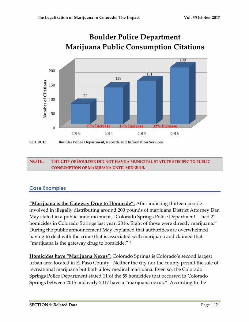
The Legalization of Marijuana in Colorado: The Impact Vol. 5/October 2017
SECTION 9: Related Data Page | 121
SOURCE: Boulder Police Department, Records and Information Services
NOTE: THE CITY OF BOULDER DID NOT HAVE A MUNICIPAL STATUTE SPECIFIC TO PUBLIC
CONSUMPTION OF MARIJUANA UNTIL MID-2013.
Case Examples
“Marijuana is the Gateway Drug to Homicide”: After indicting thirteen people
involved in illegally distributing around 200 pounds of marijuana District Attorney Dan
May stated in a public announcement, “Colorado Springs Police Department… had 22
homicides in Colorado Springs last year, 2016. Eight of those were directly marijuana.”
During the public announcement May explained that authorities are overwhelmed
having to deal with the crime that is associated with marijuana and claimed that
“marijuana is the gateway drug to homicide.” 1
Homicides have “Marijuana Nexus”: Colorado Springs is Colorado’s second largest
urban area located in El Paso County. Neither the city nor the county permit the sale of
recreational marijuana but both allow medical marijuana. Even so, the Colorado
Springs Police Department stated 11 of the 59 homicides that occurred in Colorado
Springs between 2015 and early 2017 have a “marijuana nexus.” According to the
0
50
100
150
200
2013 2014 2015 2016
72
129151
199
Nu
mb
er o
f C
itat
ion
s
Boulder Police Department
Marijuana Public Consumption Citations
17% Increase79% Increase 32% Increase

The Legalization of Marijuana in Colorado: The Impact Vol. 5/October 2017
SECTION 9: Related Data Page | 122
report, “In most cases robbery of marijuana was a motive or the victim was killed
during a marijuana narcotics transaction.” 2
Pot Deal Ends in Gunfire when Buyer Realizes they Bought Broccoli: Local Colorado
drug dealers, Tercell Davis and Sababu Colbert-Evans, “accepted $10,000 for a
marijuana sale, but Davis substituted broccoli for the pot.” Both parties had already
driven off when the buyers realized they had actually purchased broccoli instead of
marijuana. The buyers noticed they had been duped and arranged another meeting
with Davis using a different name. The next night they all met up again and “an
argument broke out, and Colbert-Evans and Davis fired 11 shots at the fleeing would-be
buyers. One was hit in the torso.” 3
Texas Trio Charged with Murder during Marijuana Robbery: Three individuals from
Texas were charged with first-degree murder while attempting to rob David Gaytan in
May 2017. The shooting that lead to the death of David Gaytan occurred at a mobile
home park in Lightner Creek, Colorado. District Attorney Christian Champagne, in a
response to the shooting, stated,
Colorado voters have clearly stated they are in favor of legalized marijuana…
which makes the state a target for people with nefarious intent from other states.
It’s a problem; I don’t know where the solution is…, I think it’s important that
we send a message that we’re taking it very seriously, and people who come
from other states to commit crimes in our community are going to be dealt with
very seriously, and that’s how we’re approaching it. 4
At Least Eleven Pot-Related Homicides Since Legalization: In response to the recent
conviction of Shawn Geerdes, an owner of a shared marijuana grow who murdered his
business partner, a local Colorado District Attorney indicated that there have been “at
least eleven pot-related homicides since legalization.” District Attorney George
Brauchler claimed that “since the passage of Amendment 64, jurisdictions across the
state have noted significant violent crime related to marijuana cultivation and
distribution.” In addition to homicide, he noted that there are additional crimes such as
“robbery, burglary, and attempted-murder cases in our community also motivated by
marijuana.” 5
Triple Homicide at Illegal Marijuana Grow: 24-year-old Garrett Coughlin was charged
with six counts of first degree murder after being accused of killing 3 people in Boulder
County. Police believed “the home was specifically targeted” by Coughlin on April 13,
2017. Witnesses told investigators they “saw Coughlin with large amounts of marijuana
packaged in a manner consistent with the marijuana owned by the victims, as well as

The Legalization of Marijuana in Colorado: The Impact Vol. 5/October 2017
SECTION 9: Related Data Page | 123
large amounts of cash following the homicides.” Over 100 plants were found at the
murder location.6, 7
A Troubling Weakness in Colorado Marijuana Enforcement: Former Colorado
Marijuana Enforcement Officer, Renee Rayton, was recently indicted due to her
involvement in shipping millions of dollars worth of marijuana outside the state.
Within weeks after leaving her state employment she was working for a shell company,
Harmony & Green. “Harmony & Green…bought legal pot cultivation licenses and
tricked investors into helping finance the scheme.” In addition to breaking state and
federal law by shipping marijuana outside of Colorado, Rayton also breached a specific
policy that prevents “former regulators from working in the industries they oversaw for
six months.”
During her time with Harmony & Green, Rayton reportedly bragged about knowing
someone at the Colorado Department of Revenue who would help the company “get
legal.” According to investigators assigned to the case, it is doubtful that she was
unaware of the “duplicitous practices that were lining her pocket,” given her vast
regulatory field experience.
Although Colorado’s Enforcement Division was correct in asking the Colorado
Bureau of Investigation to conduct an independent investigation, this example of an
Enforcement Officer gone bad highlights the complexities and challenges involved in
regulating recreational marijuana. This case made it pretty clear that the “Department
of Revenue should launch a review of its enforcement division’s practices and ensure,
through education and otherwise, that its regulators can be trusted.”8
County Official Arrested Over Illegal Pot Grow: According to investigators, Ted
Archibeque, the elected Eagle County surveyor, and his brother Thomas Archibeque are
“suspected of knowingly allowing the cultivation/manufacturing of marijuana” at an
illegal grow. Local officials and the DEA served a warrant to a property owned by Ted
Archibeque and found “28 growing plants and 65 pounds of processed marijuana” they
also observed “what appeared like recent construction of multiple greenhouses and an
airfield.” According to Kris Friel, an Eagle County spokeswoman, “Ted is still the
county surveyor” because as an elected position “there is no provision for placing the
surveyor on administrative suspension.” 9

The Legalization of Marijuana in Colorado: The Impact Vol. 5/October 2017
SECTION 9: Related Data Page | 124
Revenue
SOURCE: Governor’s Office of State Planning and Budgeting
SOURCE: Department of Revenue, Monthly Marijuana Taxes, Licenses and Fees Transfers and
Distribution, 2016
NOTE: FIGURES DO NOT INCLUDE ANY CITY TAXES; THE STATE DOES NOT ASSESS OR
COLLECT THOSE TAXES.
Colorado's Statewide Budget,
Fiscal Year 2017
Marijuana Tax Revenue*
(Medical and Recreational) = 0.8%
*Revenue from marijuana taxes as a portion of Colorado's total statewide budget
0
50,000,000
100,000,000
150,000,000
200,000,000
2.9% Regular
Sales
10% Special
Sales
15% Excise Total 2016 Taxes
23,986,490
83,750,123
59,420,537
167,157,150
12,462,467 NA NA 12,462,467
Do
llar
s
Total Revenue from Marijuana Taxes,
Calendar Year 2016Retail Marijuana Taxes Medical Marijuana Taxes

The Legalization of Marijuana in Colorado: The Impact Vol. 5/October 2017
SECTION 9: Related Data Page | 125
Case Example
Falling Marijuana Prices Mean Trouble for States that Have Legalized: As more time
elapses since marijuana legalization, prices for marijuana are expected to continue to
drop. However, states like Colorado “that tax legal marijuana sales based solely on
price” may begin to have budgetary issues. “The progression of marijuana prices over
time in Colorado perfectly parallels the pattern in Washington after that state legalized:
Prices briefly spiked due to initial supply shortages, but then began dropping as the
marijuana industry matured and expanded. Wholesale prices in Colorado tumbled 24.5
percent over the past year to $1,471 per pound.” While prices dropping may be good for
consumers it may not be good for Colorado as “sinking prices translate automatically
into sinking tax revenue per sale.” In order for Colorado to compensate for this
reduction and ensure that tax revenue remains the same, it will need to “have
substantially increased sales volume.” However, increasing consumption comes with its
own risks “such as more auto accidents by drivers who are stoned, an increase in heavy
cannabis users dropping out of school, and so on. If the state adopts measures to cut
soaring consumption, it will by definition lose tax revenue, potentially making the
recreational marijuana system unable to pay for its own regulatory costs.” 10

The Legalization of Marijuana in Colorado: The Impact Vol. 5/October 2017
SECTION 9: Related Data Page | 126
Event Planners’ Views of Denver
SOURCE: VISIT DENVER, Impacts of the Downtown Environment on the Tourism Industry and Visitor
Perceptions report
VISIT DENVER is the marketing organization for the city and it measures, records
and reports hundreds of data points, to include safety trends and feedback received
from convention and leisure visitors. Based on data collected they came away with
three key takeaways:
1. “The downtown environment is the #1 complaint from meeting planners, far
surpassing any other categories. The severity of this issue has increased and as
of 2014 nearly 50% of meeting planners negatively commented on homeless,
youth, panhandling, safety, cleanliness, and drugs including public marijuana
consumption.”
2. “Denver ranks very high on walkability, affordability, facilities, and other
factors. However, Denver as a ‘safe city’ ranks significantly lower according to
interviews with key convention planners conducted by an independent third-
party.”
3. “Denver is losing visitors and valuable convention business as a result of these
overall safety (or perception of safety) issues. Unfortunately, word is beginning
to spread among meeting planners about the safety challenges Denver is facing.
The Legalization of Marijuana in Colorado: The Impact Vol. 5/October 2017
SECTION 9: Related Data Page | 127
As the market organization for the city, we fear not being able to brand Denver
away from this growing reputation.”
Comments made by the Colorado Convention Center clients and visitors to Denver:
“I’m sorry but I would never consider putting attendees in danger by holding
a convention in your city. We are staying at Embassy Suites downtown on
16th, and last night witnessed a group of about 30 teenagers attack a man
walking along 16th street. I am told this is not an unusual occurrence. The
homeless situation is very sad, and public streets reek of weed. The Denver
police should be more alert to large groups of minors congregating on city
streets attacking tourists. My feedback from this meeting will be to never
locate here again; I have felt much safer in downtown NYC, Philly, Seattle,
and Chicago.”
“I am a 5th generation Colorado native. I am downtown for a national
convention and within 10 minutes of walking to the Convention Center I was
so disheartened: I didn’t feel safe and it was 2:00 in the afternoon. I passed
drunks, disheveled people, smelled weed being smoked in the open. It was
disgusting and I thought so this is where the current government is taking us.
I use [sic] to be so proud of Denver and Colorado; today I was heart sick and
embarrassed, knowing I’d be apologizing to colleagues coming from other
states that didn’t have sanctuary cities, legalized pot etc. Mayor Hancock,
you need to rethink what you’re doing before the Denver that was beautiful
and safe is gone.”
“This client chose to contract with the Hyatt Regency San Antonio. I would
like to share with you why Denver dropped off his list. This client does a lot
of business in Denver and was disappointed to see, in his opinion, how things
have changed in the city since marijuana was legalized. He says he sees lots
of people walking around looking ‘out of it’ and does not want to expose his
attendees to this. I hope you don’t mind the honestly [sic] but I wanted you
to know exactly ‘why’.”
“Greetings, we wanted to pass along some comments based on a national
meeting we hosted for our industry in Denver in July [2015]. It was held with
delegates arriving as early as July 11 and continued through July 15. This is a
meeting of industry executives and business owners from around the entire
country. The meeting was headquartered at the Sheraton downtown. The
chairman commented, ‘We will most likely not return to Denver based on the
current situation with all the street people.’ This was followed up by
comments from the President who echoed these comments about a reluctance
to return to Denver based on the condition of the City and the abundance of
homeless people walking the mall and in and about the downtown area. The

The Legalization of Marijuana in Colorado: The Impact Vol. 5/October 2017
SECTION 9: Related Data Page | 128
attendees were also less than complementary with Denver and in particular
the downtown area. Some of the comments received from attendee in survey
after the conference were:
o ‘Denver seems less safe now that pot is legalized.’
o ‘Don’t have a meeting in downtown Denver…what a depressing
downtown area.’
o ‘The neighborhood had way too many vagrants. I don’t remember
Denver being that bad.’
o ‘Poor area, lots of crime as we sat outside on a patio on the 16th Street
mall on Sunday evening having a beer, I turned my head to look at a
television, when I turned back a street person was drinking my beer. I
am sure this is not an image Denver wants portrayed around the
country.’”
Homeless
How Recreational Weed is attracting People, but Spiking the State’s Homeless Rate:
An article written in the summer of 2016 described the journey of a young man from a
small town in Texas to the Southern Colorado town of Pueblo. In the first half of a two-
part article, Devin Butts describes his journey to Colorado which was made largely due
to the current recreational marijuana laws. “He’d come to Colorado…because he’d
decided that cannabis would be the only indulgence he would keep as he tore himself
away from all the other, far more dangerous substances and habits he was used to.”
Devin is not alone in his journey to Colorado; in fact, there are many others that
have followed a similar fate and ended up in one of Colorado’s overcrowded homeless
shelters while trying to make a new future.
At Denver’s St. Francis Center day shelter, executive director Tom Luehrs said a
survey conducted by a grad student last year found that between 17 and 20
percent of the 350 or so new people the center was seeing each month said they’d
come to the area in part because of medical marijuana. If anything, said Luehrs
and his colleagues, that figure is low. At the nearby Salvation Army Crossroads
Shelter, an informal survey of 500 newcomers in the summer of 2014 determined
that nearly 30 percent were there because of cannabis. 11

The Legalization of Marijuana in Colorado: The Impact Vol. 5/October 2017
SECTION 9: Related Data Page | 129
Marijuana Legalization: Pot Brings Poor People to Colorado, but What’s Being Done
To Help Them?: In the second part of a summer 2016 article written to describe the
journey of a young man to Colorado, Devin Butts describes his newfound perspective.
Devin, along with hundreds of other individuals who relocated to Colorado in pursuit
of marijuana-related opportunities, found that the journey isn’t quite what he was
hoping for – especially with regards to finding employment.
The vice president of communications and public policy for the Colorado Coalition
for the Homeless spoke about hourly wage requirements to live in Denver, which is bad
news for marijuana migrants looking for work. According to Cathy Alderman,
“Workers need to make at least $19 an hour to afford housing in the Denver area. But
marijuana trimmers usually start at around $10 an hour, and budtenders working in the
dispensaries often don’t make much more than that.” This news, along with the fact
that Colorado’s housing market has been skyrocketing, seems to indicate significant
challenges for those hoping to move to Colorado in pursuit of greater futures.
Relatedly, an unexpected consequence of the legalization of recreational marijuana
is the surge in the homeless population in many Colorado cities. Recently, the city of
Aurora pledged $4.5 million in cannabis revenue to homeless programs – certainly an
unforeseen cost. Although this might seem to be a step in the right direction in order to
help those in need, it might also signal a trend in government spending and population
dependency at least partially brought-on by the legalization of recreational marijuana. 12
Denver on ‘breaking point’ with homeless population: A Salvation Army Captain
recently spoke with reporters about the growing homeless population. Captain Eric
Wilkerson said that the cause is most likely what many Denver citizens suspect, the
cause is marijuana. “People are coming here from out of state to smoke weed,” a trend
that hasn’t gone unnoticed by many of Colorado’s residents.
Additionally, “The city of Denver is not denying legal marijuana has resulted in an
increase in homelessness.” In an email from a local social services employee, it was said
that “While there isn’t a formal study on the issue, many service providers for those
experiencing homelessness tell us, anecdotally, that 20 (percent) to 30 percent of people
they encounter who are moving to Colorado tell them that they are moving here, in
part, because of legalized marijuana or to try to find work in the industry.”
Although the city of Denver has pledged large sums of money to those in need of
affordable housing, a local branding and marketing expert expressed her concern that
we get ahead of this growing trend as the last thing she wants is for her city to have the
perception of a “homeless problem.” 13
Legalized Marijuana Turns Colorado Resort Town into Homeless Magnet: Several
people holding cardboard signs can be seen lining the sidewalks and streets of
Durango, CO. Durango is a picturesque, upscale community where many businesses

The Legalization of Marijuana in Colorado: The Impact Vol. 5/October 2017
SECTION 9: Related Data Page | 130
rely on tourism. The city has recently become overrun with transients and panhandlers,
many of them people between the ages of 20-30. One resident and business owner
mentioned “most of the kids here are from out of state, and I would say it has a lot to do
with the legalized pot.” The small city has also experienced an increase in crime,
placing its property crime rate 12 percent higher than the national average.14
Suicide Data
SOURCE: Colorado Department of Public Health and Environment (CDPHE), Colorado Violent Death
Reporting System
0.00% 5.00% 10.00% 15.00% 20.00%
Marijuana
Alcohol
Amphetamine
Cocaine
Opioid
Antidepressant
16.30%
8.70%
4.70%
2.30%
4.70%
4.70%
17.40%
11.70%
2.30%
1.90%
6.60%
4.20%
13.50%
12.00%
3.80%
0.00%
0.00%
3.80%
Percent
Average Toxicology of Suicides Among
Adolescents Ages 10 to 19 Years Old(With Known Toxicology)
2006-2008
Pre-Commercialization
2009-2012
Post-Commercialization
2013-2015
Legalization

The Legalization of Marijuana in Colorado: The Impact Vol. 5/October 2017
SECTION 9: Related Data Page | 131
SOURCE: Colorado Department of Public Health and Environment (CDPHE), Colorado Violent Death
Reporting System
Marijuana is the only substance where youth, ages 10 to 19, have a
higher percentage than adults, ages 20 and older.
0%
5%
10%
15%
20%
25%
30%
35%
40%
Marijuana Alcohol Amphetamine Cocaine Opiod Antidepressant
16.3%
8.7%
4.7%2.3%
4.7% 4.7%
15.8%
38.6%
6.8%
2.8%
20.0%17.4%
Per
cen
t o
f S
uic
ides
Average Toxicology Results by Age Group,
2013-2015
Ages 10 to 19 Ages 20+

The Legalization of Marijuana in Colorado: The Impact Vol. 5/October 2017
SECTION 9: Related Data Page | 132
THC Potency
SOURCE: Potency Monitoring Program, Quarterly Report Number 135, National Center for Natural
Products Research (NCNPR) at the University of Mississippi, under contract with the National
Institute on Drug Abuse.
The average potency for buds/flower in Colorado is 17.1 percent. 15
3.96%
4.51%
5.01%
4.91%
4.60%
5.34%
6.11%
7.20%
7.15%
8.14%
8.02%
8.76%
9.58%
9.93%
9.75%
10.36%
11.13%
12.27%
11.99% 12.09%
11.04%
0.00%
2.00%
4.00%
6.00%
8.00%
10.00%
12.00%
14.00%19
95
1996
1997
1998
1999
2000
2001
2002
2003
2004
2005
2006
2007
2008
2009
2010
2011
2012
2013
2014
2015
Av
erag
e T
HC
Per
cen
t
National Average THC Potency
Submitted Cannabis Samples

The Legalization of Marijuana in Colorado: The Impact Vol. 5/October 2017
SECTION 9: Related Data Page | 133
SOURCE: Potency Monitoring Program, Quarterly Report Number 135, National Center for Natural
Products Research (NCNPR) at the University of Mississippi, under contract with the National
Institute on Drug Abuse.
The average potency for concentrates in Colorado is 62.1 percent. 15
13.23%
12.82%
18.20%
15.78%
16.21%
28.58%
19.44%
22.51%
15.54%
31.32%
6.40%
18.74%
24.85%
6.73%
12.71%
36.16%
35.28%
53.52%
49.98%
50.79%
55.85%
0.00%
10.00%
20.00%
30.00%
40.00%
50.00%
60.00%19
95
1996
1997
1998
1999
2000
2001
2002
2003
2004
2005
2006
2007
2008
2009
2010
2011
2012
2013
2014
2015
Av
erag
e T
HC
Per
cen
t
National Average THC Potency
Submitted Hash Oil Samples

The Legalization of Marijuana in Colorado: The Impact Vol. 5/October 2017
SECTION 9: Related Data Page | 134
Alcohol Consumption
It has been suggested that legalizing marijuana would reduce alcohol
consumption. Thus far that theory is not supported by the data.
SOURCE: Colorado Department of Revenue, Colorado Liquor Excise Tax
SOURCE: Colorado Department of Revenue, Colorado Liquor Excise Tax
130,000,000
132,000,000
134,000,000
136,000,000
138,000,000
140,000,000
142,000,000
144,000,000
Pre-Legalization
2010-2012
Post-Legalization
2013-2016
136,364,158
143,777,836
Gal
lon
s
Colorado Average Consumption of Alcohol
130,000,000
132,000,000
134,000,000
136,000,000
138,000,000
140,000,000
142,000,000
144,000,000
146,000,000
148,000,000
2010 2011 2012 2013 2014 2015 2016
135,824,179
136,778,438
136,489,856
143,468,372
141,184,231142,970,403
147,488,339
Gal
lon
s
Colorado Consumption of Alcohol
Legalization
5% Increase

The Legalization of Marijuana in Colorado: The Impact Vol. 5/October 2017
SECTION 9: Related Data Page | 135
Medical Marijuana Registry 16
Medical Marijuana Registry Identification Cards
December 31, 2009 – 41,039
December 31, 2010 – 116,198
December 31, 2011 – 82,089
December 31, 2012 – 108,526
December 31, 2013 – 110,979
December 31, 2014 – 115,467
December 31, 2015 – 107,534
December 31, 2016 – 94,577
Profile of Colorado Medical Marijuana Cardholders:
Age of cardholder
o 63 percent male, with an average age of 43 years
o 0.3 percent between the ages of 0 and 17
o 46 percent between the ages of 18 and 40
21 percent between the ages of 21 and 30
Reporting medical condition of cardholder
o 93 percent report severe pain as the medical condition
o 6 percent collectively report cancer, glaucoma and HIV/AIDS
o 3 percent report seizures

The Legalization of Marijuana in Colorado: The Impact Vol. 5/October 2017
SECTION 9: Related Data Page | 136
SOURCE: Colorado Department of Public Health and Environment, Medical Marijuana Statistics
NOTE: TOTAL DOES NOT EQUAL 100 PERCENT AS SOME PATIENTS REPORT USING MEDICAL
MARIJUANA FOR MORE THAN ONE DEBILITATING MEDICAL CONDITION.
0%
10%
20%
30%
40%
50%
60%
70%
80%
90%
100%
Cachexia Cancer Glaucoma HIV /
AIDS
Muscle
Spasms
Seizures Sever
Nausea
Severe
Pain
1% 4% 1% 1%
25%
3%
13%
93%
Per
cen
t o
f P
ati
ents
Percent of Medical Marijuana Patients Based
on Reporting Conditions, 2016

The Legalization of Marijuana in Colorado: The Impact Vol. 5/October 2017
SECTION 9: Related Data Page | 137
Colorado Licensed Marijuana Businesses as of August 1st, 2017 17
Medical Marijuana:
759 marijuana cultivation facilities
507 medical marijuana centers (dispensaries)
255 infused products (edibles) businesses
14 testing facilities
Recreational Marijuana:
701 marijuana cultivation facilities
498 marijuana retail stores
273 infused product (edibles) businesses
13 testing facilities
Business Comparisons, June 2017
Figures for business comparisons were all acquired by June of 2017 for
comparable data.
SOURCE: Colorado Department of Revenue; Starbucks Coffee Company, Corporate Office Headquarters;
McDonalds Corporation, Corporate Office Headquarters
0
100
200
300
400
500
600
McDonalds Starbucks Retail Marijuana
Stores
Medical
Marijuana
Dispensaries
208
392
491513
Lic
ense
d B
usi
nes
ses
Colorado Business Comparisons, June 2017

The Legalization of Marijuana in Colorado: The Impact Vol. 5/October 2017
SECTION 9: Related Data Page | 138
Demand and Market Size 18
The Colorado Department of Revenue published a report in July 2014 called, “Market
Size and Demand for Marijuana in Colorado.” A follow-up to this report showed data
for 2015. Some of the information included:
Demand
In 2015, the established demand for marijuana by Colorado residents 21 years
and older is 134.7 metric tons (296,962.67 pounds) of marijuana.
In 2015, the estimated demand for marijuana by out-of-state visitors 21 years and
older is 14.0 metric tons (30,864.7 pounds).
Market Size
There are an estimated 569,000 Colorado adult regular marijuana users (at least
once per month).
Heavy users who consume marijuana nearly daily make up less than 25 percent
of the user population but account for 76.4 percent of the demand for marijuana.

The Legalization of Marijuana in Colorado: The Impact Vol. 5/October 2017
SECTION 9: Related Data Page | 139
Marijuana Enforcement Division Reported Sales of Marijuana in Colorado 19, 20
In 2015:
144,537 pounds of medical marijuana flower
106,932 pounds of recreational marijuana flower
2,261,875 units of medical edible products
5,280,297 units of recreational edible products
In 2016:
159,998 pounds of medical marijuana flower
175,642 pounds of recreational marijuana flower
2,117,838 units of medical edible products
7,250,936 units of recreational edible products
A single ounce of marijuana, depending on the solvent type and production
method, can produce “between 347 and 413 edibles of 10 mg [THC] strength.”15
2017 Price of Marijuana
Marijuana prices as of July 2017 are based off a compilation of medical and recreational
prices from local dispensaries and averaged:
Area Gram Ounce
State Average $11.00 $191.00
Denver $11.00 $159.00
Boulder $13.00 $213.00
Fort Collins $11.00 $235.00
Colorado Springs* $8.00 $157.00
*Colorado Springs does not allow selling of recreational marijuana within city limits.
SOURCE: “Colorado marijuana prices for July 2017,” Marijuanarates.com, Accessed August 29, 2017

The Legalization of Marijuana in Colorado: The Impact Vol. 5/October 2017
SECTION 9: Related Data Page | 140
Local Response to Medical and Recreational Marijuana in Colorado
Recreational Marijuana Business and Local Jurisdiction Response: 21, 22
SOURCE: Colorado Counties, Inc.; as of August 4th, 2017
*NOTE: THIS MAP SHOWS THE REGULATORY STATUSES OF UNINCORPORATED AREAS WITHIN
EACH COUNTY. MUNICIPALITIES WITHIN EACH COUNTY SET POLICY WITHIN THEIR
BOUNDARIES.
64 counties*
o 61 percent have prohibited or have a moratorium (39)
o 39 percent have allowed (25) * Broomfield and Denver are both a city and county but included only once in county data.
243 municipalities (cities and incorporated areas) have taken action on the issue
o 72 percent have prohibited (167) or have a moratorium (8)
o 28 percent have allowed (68)
*

The Legalization of Marijuana in Colorado: The Impact Vol. 5/October 2017
SECTION 9: Related Data Page | 141
Medical Marijuana Business and Local Jurisdiction Response: 21, 22
SOURCE: Colorado Counties, Inc.; as of July 31, 2017
*NOTE: THIS MAP SHOWS THE REGULATORY STATUSES OF UNINCORPORATED AREAS WITHIN
EACH COUNTY. MUNICIPALITIES WITHIN EACH COUNTY SET POLICY WITHIN THEIR
BOUNDARIES.
64 counties*
o 59 percent have prohibited or have a ban on new businesses (38)
o 41 percent have allowed (26) * Broomfield and Denver are both a city and county but included only once in county data.
177 municipalities have taken action on the issue
o 65 percent have prohibited (115)
o 35 percent have allowed (62)

The Legalization of Marijuana in Colorado: The Impact Vol. 5/October 2017
SECTION 9: Related Data Page | 142
Local Jurisdictions Reporting Marijuana Licensing Status
as of December 31, 2016 20
Medical and Retail Marijuana Banned 212
Medical Marijuana Licenses Only 18
Retail Marijuana Licenses Only 11
Medical and Retail Marijuana Licenses 79
SOURCE: Marijuana Enforcement Division, 2016 Annual Update
For Further Related Data See Page 158
66%6%
3%
25%
2016 Local Jurisdiction Licensing Status
Medical and Retail Banned
Medical Only
Retail Only
Medical and Retail Allowed

The Legalization of Marijuana in Colorado: The Impact Vol. 5/October 2017
SECTION 9: Related Data Page | 143
Sources:
1 Colorado Springs, Colo. (KKTV), “Black market marijuana bust leaves bruises on
Colorado’s marijuana industry,” July 25, 2017,
<http://www.kktv.com/content/news/Black-market-marijuana-bust-leaves-bruises-on-
Colorados-marijuana-industry-436622893.html>, accessed July 31, 2017.
2 Blair Miller, “Colorado Springs Police: 18 Percent of Homicides Since 2015 Have
‘Marijuana Nexus’; No State Data.” Denver Channel, March 15th, 2017,
<http://www.thedenverchannel.com/news/local-news/colorado-springs-police-18-
percent-of-homicides-since-2015-have-marijuana-nexus-no-state-data>, accessed August
29th, 2017.
3 Kieran Nicholson, “Bogus pot deal, involving broccoli, and gunfire at Aurora mall
gets man 16 years in prison,” Denver Post,
<http://www.denverpost.com/2017/07/25/aurora-marijuana-deal-broccoli-town-center-
gunfire-sentenced/>, accessed September 12th, 2017.
4 Shane Benjamin, “Texas trio charged with first-degree murder in Lightner Creek
shooting,” Durango Herald, <https://durangoherald.com/articles/164814-texas-trio-
charged-with-first-degree-murder-in-lightner-creek-shooting>, accessed September 12th,
2017.
5 George Brauchler, “At Least Eleven Pot-Related Homicides Since Legalization, DA
Says,” Westword, < http://www.westword.com/news/marijuana-related-homicides-in-
colorado-since-legalization-9345285>, accessed September 12th, 2017.
6 Mitchel Byars, “Suspect in Coal Creek Canyon Triple Homicide To Appear in
Court Thursday,” Daily Camera, <http://www.dailycamera.com/boulder-county-
news/ci_30994865/suspect-coal-creek-canyon-triple-homicide-appear-
court?source=pkg>, accessed September 11, 2017.
7 Mitchel Byars, “Garrett Coughlin Charged With 6 Murder Counts in Coal Creek
Canyon Killings,” Daily Camera, <http://www.dailycamera.com/boulder-county-
news/ci_30996366/suspect-coal-creek-canyon-triple-homicide-charged-six?source=pkg>,
accessed September 11, 2017.
8 The Denver Post Editorial Board, “A troubling weakness in Colorado Marijuana
enforcement,” June 16, 2017, The Cannabist,

The Legalization of Marijuana in Colorado: The Impact Vol. 5/October 2017
SECTION 9: Related Data Page | 144
<http://www.thecannabist.co/2017/06/16/colorado-marijuana-enforcement-indictment-wakeup-
call/82104/>, accessed September 21, 2017. 9 Jesse Paul, “Eagle County official and his brother arrested in connection with
illegal marijuana grow,” The Denver Post, December 8, 2016,
<http://www.denverpost.com/2016/12/08/eagle-county-official-brother-arrested-illegal-
marijuana-grow/>, accessed September 22, 2017.
10 Keith Humphreys, “Falling marijuana prices mean trouble for states that have
legalized,” The Washington Post, January 18th, 2017,
<http://www.thecannabist.co/2017/01/18/marijuana-price-drops-state-revenue/71657/>,
accessed August 3rd, 2017.
11 Joel Warner, “Marijuana Legalization in Colorado: How Recreational Weed Is
Attracting People, But Spiking The State’s Homeless Rate {PART ONE}, International
Business Times, June 20, 2016, <http://www.ibtimes.com/marijuana-legalization-
colorado-how-recreational-weed-attracting-people-spiking-2374204>, accessed October
9, 2016.
12 Joel Warner, “Marijuana Legalization: Pot Brings Poor People To Colorado, But
What’s Being Done To Help Them? {PART TWO}, International Business Times, June 21,
2016, <http://www.ibtimes.com/marijuana-legalization-pot-brings-poor-people-
colorado-whats-being-done-help-them-2378769>, accessed October 9, 2016.
13 Joe St. George, “Salvation Army: Denver on ‘breaking point’ with homeless
population, Fox31 Denver, July 7, 2016, <http://kdvr.com/2016/07/07/salvation-army-
denver-on-breaking-point-with-homeless-population/>, accessed October 9, 2016.
14 Joseph J. Kolb, “Legalized marijuana turns Colorado resort town into homeless
magnet,” FoxNews.com, May 17, 2017,
<http://www.foxnews.com/us/2017/05/17/legalized-marijuana-turns-colorado-resort-
town-into-homeless-magnet.html>, accessed May 17, 2017.
15 Marijuana Policy Group, “Marijuana Equivalency in Portion and Dosage (as of
August 10th, 2015),”
<https://www.colorado.gov/pacific/sites/default/files/MED%20Equivalency_Final%2008
102015.pdf>, accessed May 12th, 2017.
16 Colorado Department of Public Health and Environment, “Medical Marijuana
Registry Program Update (as of December 31st, 2016),”

The Legalization of Marijuana in Colorado: The Impact Vol. 5/October 2017
SECTION 9: Related Data Page | 145
<https://www.colorado.gov/pacific/sites/default/files/CHED_MMR_Report_December_
2016.pdf> accessed May 12th, 2017.
17 Colorado Department of Revenue, “Licensees – Marijuana Enforcement Division
(As of August 1st, 2017),” < https://www.colorado.gov/pacific/enforcement/licensees-
marijuana-enforcement-division>, accessed August 31, 2017.
18 Marijuana Policy Group, “The Economic Impact of Marijuana Legalization in
Colorado,” Marijuana Enforcement Division, received August 1, 2017.
19 Marijuana Enforcement Division, “MED 2015 Annual Update,” Colorado
Department of Revenue, September 26, 2016.
20 Marijuana Enforcement Division, “MED 2016 Annual Update,” Colorado
Department of Revenue, August 2, 2017.
21 Colorado Municipal League, “Municipal Retail Marijuana Status,”
<http://www.cml.org/rmj-action-visual/, accessed 8/29/2017>.
22 Colorado Counties Inc., <ccionline.org>, August 28, 2017.

The Legalization of Marijuana in Colorado: The Impact Vol. 5/October 2017
SECTION 9: Related Data Page | 146
THIS PAGE INTENTIONALLY LEFT BLANK

The Legalization of Marijuana in Colorado: The Impact Vol. 5/October 2017
SECTION 10: Reference Materials Page | 147
SECTION 10: Reference
Materials
Reports and Articles
Impaired Driving
Higher Levels of THC: In Colorado, the legal limit of THC in a driver’s blood is
5ng/mL. However, according to the Denver Post, “THC levels in drivers killed in
crashes in 2016 routinely reached levels of more than 30 ng/mL… [t]he year before,
levels only occasionally topped 5 ng/mL.” This trend has coroners concerned because
some are “uncertain about listing the presence of THC on a death certificate because of
doubts on what constitutes impairment.” Police Chief Jackson of Greenwood Village,
CO attributes the rise in THC levels of drivers to the rise in THC potency in marijuana
oils and concentrates. He states, “This is not your grandfather’s weed.” 1
Cannabis-Impaired Driving is a Public Health and Safety Concern: According to a
2015 study which aimed to examine some of the issues surrounding cannabis impaired
driving, “The percentage of weekend nighttime drivers with measureable Δ9-
tetrahydrocannabinol (THC) in blood or oral fluid increased to 12.6%, a 48% increase
since 2007.” With the recent recreational legalization of marijuana in multiple states, this
is likely a national trend we will see continue in the years to come. 2
Controlled Cannabis Vaporizer Administration with and without Alcohol:
Researchers behind a 2015 study examined the vaporization of cannabis both with and
without blood alcohol present in the systems of thirty-two regular cannabis smokers. As
noted in the Clinical Chemistry article, smoking is the most common administration
route of cannabis but the use of vaporization is increasing rapidly. The conclusions
section of the study stated that the significantly higher blood THC concentration values
in combination with blood alcohol “possibly explain[s] increased impairment observed
from cannabis-alcohol combinations.” The conclusions of this study further underscore
the complexities and issues that need to be closely examined, especially when
considering drugged driving legislation. 3
The Legalization of Marijuana in Colorado: The Impact Vol. 5/October 2017
SECTION 10: Reference Materials Page | 148
Correlates of Marijuana Drugged Driving and Openness to Driving While High: A
2015 study funded and independently conducted by RTI International, a nonprofit
research and technical services organization, examined 865 Colorado and Washington
residents who self-reported using marijuana in the past 30 days. Two behaviors were
looked at among the group of study participants; any instances of driving while high in
the last year, and driving within 1 hour of using marijuana 5 or more times in the past
month.
Researchers found that the “Prevalence of past-year driving while under the
influence of marijuana was 43.6% among respondents.” Additionally, “The prevalence
of driving within 1 hour of using marijuana at least 5 times in the past month was
23.9%.”
Furthermore, it was concluded that “Interventions for reducing the incidence of
marijuana DUI are likely to be more successful by targeting safety perceptions related
to marijuana DUI rather than knowledge of DUI laws.” 4
A 2-Year Study of THC Concentrations in Drivers: A recent study aimed to examine
police and Drug Recognition Expert (DRE) evaluations with regards to driving under
the influence of marijuana. Researchers hoped to determine whether or not a correlation
exists between whole-blood THC concentrations and field sobriety test performance.
“As suspected, the findings of this study did not find a correlation between
performance on field sobriety tests and the concentration of THC tested in whole-blood
samples.” This information further adds to the discussion around marijuana use and
permissible driving limits. Much more research is needed in order to come up with
appropriate marijuana driving laws/legislation throughout the country.
Furthermore, the researchers concluded that, “The driving behaviors seen in THC-
impaired drivers are similar to those seen in alcohol-impaired drivers.” Contrary to
anecdotal accounts of “high” drivers being slow and cautious drivers, the most often
observed driving behaviors of study participants included speeding, the inability to
maintain lane position, and running red lights or stop signs. 5
57 Percent of Marijuana Users in Colorado Admit Driving within 2 Hours: A survey
conducted by the Colorado Department of Transportation discovered that 57 percent of
people who reported using marijuana drove within two hours after consumption. The
survey also indicated that, on average, those participants who reported consuming
marijuana and then driving within 2 hours did so on 11.7 of 30 days. By comparison, 38
percent of respondents who drank alcoholic beverages reported driving within 2 hours
after consumption and only reported doing so on 2.8 of 30 days. 6
DRE Examination Characteristics of Cannabis Impairment: The frequently-debated
5ng/mL blood THC per se cutoff has been the source of much controversy since

The Legalization of Marijuana in Colorado: The Impact Vol. 5/October 2017
SECTION 10: Reference Materials Page | 149
legalized marijuana has hit the scene. In 2016, a study of Drug Recognition Expert
(DRE) characteristics of cannabis impairment further highlighted the “limited
relevance” of the 5ug/L cutoff. “Combined observations on psychophysical and eye
exams produced the best cannabis-impairment indicators.” Additionally, “No
significant differences were detected between cases with blood THC >5ng/mL versus
<5ng/mL.” More specifically the finger-to-nose test was seen as the best indicator of
cannabis impairment, with the values of sensitivity, specificity, predictive value and
efficiency being considered. 7
Smoked Cannabis Psychomotor and Neurocognitive Effects in Occasional and
Frequent Smokers: A group of researchers interested in examining the severity of
psychomotor performance, cognition, and driving ability differences among frequent
and occasional users of cannabis found substantial differences among the frequent users
and the occasional users. During the study, “fourteen frequent (equal or greater than
4x/week) and 11 occasional (less than 2x/week) cannabis smokers entered a secure
research unit approximately 19 hours prior to smoking one 6.8% THC cigarette.”
Cognitive and psychomotor performance was measured in a variety of ways at certain
intervals of time both prior to and after the drug use.
Researchers concluded that there are “significant differences between occasional and
frequent cannabis smokers in psychomotor, subjective and physiological effects
following cannabis smoking, with weaker effects in frequent smokers suggesting
tolerance development. Impairment domains included those that play a key role in
driver’s ability to accurately control a car or to react to events on the road.” 8
Time Profile of Serum THC Levels in Occasional and Chronic Marijuana
Users after Acute Drug Use: Although it is commonly accepted that cannabis
consumption has the ability to influence cognitive and psychomotor functions,
the rules on how to assess the ability to drive while under the influence of
cannabis are not very clear. “The psychoactive compound delta-9-
tetrahydrocannabinol (THC) impairs cognition, psychomotor behavior and
driving performance in a dose-related manner approximately.” After researching
the time profile related to cannabis consumption and the related physiologic
affects (through observation of human volunteers), it is apparent that there is
“great individual variability of the kinetic profile of THC in blood…” The
research article goes on to describe that “Low blood concentrations of THC close
to the limit of detection… are justified in an effective traffic legislation.” 9
Effect of Blood Collection Time: Drug testing is a highly scrutinized topic when it
comes to marijuana use and the operation of motor vehicles. This topic has been made
even more controversial as several states have legalized marijuana for medical and/or

The Legalization of Marijuana in Colorado: The Impact Vol. 5/October 2017
SECTION 10: Reference Materials Page | 150
recreational use. Therefore, a group of researchers examined the impact of blood
collection time on toxicological evaluation for THC.
Researchers found that blood THC concentrations at the time of driving cannot be
reliably determined due to individual variances. 10
Drivers Killed in Crashes More Likely to be on Drugs than Alcohol: A recent
study using data available from 2015 indicates that “[d]rivers who are killed in car
crashes are now more likely to be on drugs than alcohol.” Drugs were present in 43
percent of drivers in fatal accidents compared to 37 percent with alcohol above the legal
limit. Additionally, 36 percent of the drivers tested had marijuana present in their
system at the time of the accident. In general, traffic fatalities are rising and can be
attributed to factors such as improved economy, more distracted drivers, and more
drugged drivers. 11
Drug-impaired Driving: In this report, Dr. James Hedlund, under contract with the
Governors Highway Safety Association (GHSA), described “the current state of
knowledge on drug-impaired driving, including what little is known about the costs
and effectiveness of these actions, and identifies actions states can take to reduce drug-
impaired driving.” The report cites a variety of sources, including the Fatality Analysis
and Reporting System (FARS) and various roadside surveys conducted in multiple
states. Through these data sources, Dr. Hedlund determined “marijuana is by far the
most common drug that is used.” He also described that while drug-impaired driving
is more complex than alcohol-impaired driving, “43% of fatally-injured drivers with
known test results tested positive for drugs or marijuana in 2015, more than tested
positive for alcohol”. The report pointed out additional differences between alcohol-
impaired driving and drug-impaired driving and made recommendations for states to
enact education programs, legislation, and officer training programs. 12

The Legalization of Marijuana in Colorado: The Impact Vol. 5/October 2017
SECTION 10: Reference Materials Page | 151
Youth Marijuana Use
Marijuana Use up among Teens since Legalized in Colorado, Washington:
Researchers at the University of California Davis and Columbia University Mailman
School of Public Health conducted a study involving teens’ perception of marijuana use
before and after recreational marijuana was legalized in their state. The study, which
used nation-wide data of nearly 254,000 students who participated in the Monitoring
the Future survey, showed that legalization of recreational marijuana significantly
reduced perceptions of marijuana’s harmfulness by 14 percent in 8th graders and 16
percent in 10th graders in Washington state but not in Colorado. Researchers attribute
the lack of change in perception in Colorado to the state’s robust medical marijuana
industry that was established prior to recreational legalization. Youth were exposed to
substantial advertising from the medical marijuana industry and therefore Colorado
has had lower rates of perceived harmfulness and higher rates of use compared to
Washington state and other states. The researchers recommend that states considering
legalizing recreational marijuana should also consider investing in substance abuse
prevention programs for adolescents. 13
Pot Smoking Common among Pregnant Teens: A recent national survey given to
approximately 14,400 pregnant women aged 12-44, found “more than twice as many
pregnant 12- to 17-year-olds use marijuana as their non-pregnant peers.” This
constituted 14% of the surveyed mothers-to-be. Teen pregnancies are already
“associated with smaller babies,” but there may be other risks to a pregnancy caused by
marijuana use. According to Dr. Judy Chang, associate professor of obstetrics,
gynecology and reproductive sciences at the University of Pittsburgh, “some of the
studies that do exist suggest that there are risks to the pregnancy from pot use.” Some
of those risks may include “scrawnier babies, kids who have some problems with their
thinking and learning abilities, [and] kids who find it harder to do more complicated
brain tasks when they are teenagers.” Additional evidence may suggest that “there
could be a risk of causing brain damage in a developing baby,” and that the
tetrahydrocannabinol (THC) “may also influence neural development and brain
maturation,” which could lead to a “long-term risk for addiction.” 14
Unintentional Pediatric Exposures to Marijuana in Colorado, 2009-2015: Colorado
researchers examined the effects of the legalization of marijuana on youth in Colorado
by analyzing data regarding pediatric marijuana exposures. Specifically, researchers set
out to compare the incidence of pediatric marijuana exposures before and after
recreational marijuana legalization. Additionally, this study compared Colorado data
with nationwide data.

The Legalization of Marijuana in Colorado: The Impact Vol. 5/October 2017
SECTION 10: Reference Materials Page | 152
It was found that cases for pediatric marijuana exposure increased significantly and
at a higher rate than the rest of the United States. “Almost half of the patients seen in
the children’s hospital in the 2 years after legalization had exposures from recreational
marijuana, suggesting that legalization did affect the incidence of exposures.” 15
Pediatricians Warn against Use of Pot: A report released in 2017 from the American
Academy of Pediatrics describes why many doctors are now “beefing up warnings
about marijuana’s potential harms for teens amid increasingly lax laws and attitudes on
pot use.” This report states that the group “opposes medical and recreational marijuana
use for kids.” A youth’s brain continues to develop through their early 20s, so “the
potential short-term and long-term effects of a mind-altering drug” are of great concern.
Some of these effects may even be permanent. This is particularly true for frequent
users who begin at an early age. “Teens who use marijuana at least 10 times a month
develop changes in brain regions affecting memory and the ability to plan” as well as
lowered IQ scores in some cases. Also some studies have shown that “starting
marijuana use at a young age is more likely to lead to addiction than starting in
adulthood.” These doctors stress that messaging is particularly important because
according to government data “kids 12-17 increasingly think marijuana use is not
harmful.” 16
Adult Marijuana Use
Study Finds Increase in Illicit Pot Use, Abuse in States that Allow Medical
Marijuana: “In a study published in the Journal of American Medical Association
(JAMA) Psychiatry, researchers noted a significant increase in illegal cannabis use and
so-called cannabis-use disorders in states with medical marijuana laws” Although a
small minority of the population might potentially benefit from medical marijuana use,
this study aims to quantify how much non-medical, illicit use is taking place over a
multi-year timespan. The research study defined illegal or illicit use as “obtaining
marijuana not from a prescription or a dispensary with the intent of getting high.”
Those with cannabis-use disorders are described as having withdrawal symptoms,
developing a tolerance for the drug, having cravings for the drug, and suffering
impaired functioning in daily activities.
The lead author of the study, Dr. Deborah Hasin of the Columbia University
Mailman School of Public Health said “[Americans have] come to see cannabis as a
harmless drug or harmless substance.” More education is certainly needed on the risks
associated with marijuana use.

The Legalization of Marijuana in Colorado: The Impact Vol. 5/October 2017
SECTION 10: Reference Materials Page | 153
The study examined cannabis use and cannabis use disorder from 1991-1992
through 2012-2013 timeframes. In the Washington Times article, Dr. Hasin said “I was
somewhat surprised with rates that increased so sharply in Colorado and California,
who most experienced increase in dispensaries in 2009 and 2010.” 17
Drug Positivity in U.S. Workforce Rises to Nearly Highest Level in a Decade:
According to the world’s leading provider of diagnostic drug testing services, “The
percentage of employees in the combined U.S. workforce testing positive for drugs has
steadily increased over the last three years to a 10-year high.” The three primary
diagnostic tests offered by Quest Diagnostics include oral, urine and hair follicle drug
tests. Speaking to oral fluid testing, which provides a 24-48 hour history, the positivity
rate increased 47 percent in the past three years. According to the diagnostics
corporation, “The increase was largely driven by double-digit increases in marijuana
positivity during this time period. In 2015, there was a 25 percent relative increase in
marijuana detection as compared to 2014.” Additionally, “Almost half (45 percent) of
individuals in the general U.S. workforce with a positive drug test for any substance in
2015 showed evidence of marijuana use. 18
Marijuana is Not Safe to Smoke: A study conducted by UC Davis academics found
multiple bacterial and fungal pathogens in marijuana that can cause serious infections.
The weed tested originated from Northern California dispensaries where the
Department of Public Health is working on guidelines for marijuana testing to ensure
marijuana is safe. George Thompson III, an associate professor of clinical medicine at
the university who helped conduct the study, stressed that “there really isn’t a safe way
to smoke marijuana buds, even for those who are healthy”. Inhaling marijuana smoke
leads the pathogens directly into the lungs where they can cause serious illness and
even death. 19
These College Students Lost Access to Legal Pot – and Started Getting Better Grades:
A recent study out of the Netherlands found that “college students with access to
recreational cannabis on average earn worse grades and fail classes at a higher rate.”
Due to a new policy change to cannabis cafes, noncitizens were barred from buying
recreational marijuana from the cafes. Due to this policy change, an experiment
regarding college students and marijuana use was conducted. “The research on more
than 4,000 students… found that those who lost access to legal marijuana showed
substantial improvement in their grades. Specifically, those banned from cannabis cafes
had a more than 5 percent increase in their odds of passing their courses.” 20
More U.S. Women Report Using Marijuana during Pregnancy, Amid Uncertainty on
Potential Harms: About 4 percent of pregnant women ages 18 to 44 reported using

The Legalization of Marijuana in Colorado: The Impact Vol. 5/October 2017
SECTION 10: Reference Materials Page | 154
marijuana during pregnancy. The study conducted between 2002 and 2014 showed an
increase of 62 percent from numbers in 2002 to numbers in 2014. Pregnant women are
turning towards marijuana to help alleviate nausea caused during pregnancy even
though it is discouraged by the American College of Obstetricians and Gynecologists.
Studies show links between prenatal marijuana exposure and impaired functions such
as impulse control, visual memory, and attention during school years. Other studies
showed smoking marijuana during pregnancy may also lead to restricted fetal growth
during pregnancy as well as increased frontal cortical thickness among school-aged
children. 21
Pregnant Women Turn to Marijuana, Perhaps Harming Infants: Doctors and
researchers are concerned that due to “an increased perception of the safety of cannabis
use, even in pregnancy,” it is becoming more common for people to “presume that
cannabis has no consequences for developing infants.” Evidence on the effects of
prenatal marijuana use has been limited up to this point, which may contribute to the
false perception of safety by some. However, preliminary research indicates that
marijuana’s psychoactive ingredient, tetrahydrocannabinol (THC), can cross the
placenta and reach the fetus potentially harming development. In addition, because
THC is stored in fat and can linger there for weeks or months, breast milk can contain
THC.
Despite evidence being limited, several studies linking maternal marijuana use have
found “changes in the brains of fetuses, 18 to 22 weeks old.” Additional studies
conducted in Pittsburgh and Ottawa show that children whose mothers used marijuana
heavily in the first trimester may have difficulty “understand[ing] concepts in listening
and reading,” and had “lower scores in reading, math and spelling… than their peers.”
Much of the research that has been done in this area was done when marijuana was far
less potent. An epidemiologist with the University of Washington stated “all those
really good earlier studies on marijuana effects aren’t telling us what we need to know
now about higher concentration levels.” Not much is known about the lingering effects
of marijuana, and whether or not the fetus’s exposure is limited to the time a mother
feels high. Both the American Academy of Pediatrics and the American College of
Obstetricians and Gynecologists advise expecting mothers against the use of cannabis
during pregnancy citing cognitive impairment and academic underachievement as
areas of concern. 22
Causal Relationship Identified between Marijuana Use and Numerous Fetal Issues
during Pregnancy: Since 2002, there has been a 62% increase in pregnant marijuana
users. “Estimates suggest that marijuana use complicates 2% to 5% of all pregnancies”
in the United States. The amount of studies regarding marijuana use is limited due to
the drug’s complicated legal status. However, “evidence has identified a causal

The Legalization of Marijuana in Colorado: The Impact Vol. 5/October 2017
SECTION 10: Reference Materials Page | 155
relationship between marijuana use and decreased birth weight, increased spontaneous
abortion, impaired neurodevelopment, and functional deficits among children and
adults who were exposed [to marijuana] in utero.” It is not yet known how exactly fetal
development is effected by marijuana which leads obstetricians and gynecologists to
“urge their patients who are pregnant or contemplating pregnancy to discontinue
marijuana use.” Further concern for the effects of marijuana during pregnancy are
warranted “due to its lipophilic nature, [it] can easily cross the blood brain barrier and
enter the placenta.” Additionally, the nature of Tetrahydrocannabinol (THC) is such
that it can remain in maternal blood for weeks and “[a]s a result, occasional use of
marijuana during pregnancy, as little as once per month, results in fetal exposure that
persists throughout the pregnancy.” 23
Emergency Department and Hospital Marijuana-Related Admissions
Marijuana Abuse Linked to Increased Myocardial Infarction (MI) Risk: Cardiology
News recently published an article about marijuana being linked with an “eye-opening
doubled risk of acute MI.” Myocardial infarction (MI) is more commonly known as a
heart attack.
The March 2017 article summarized the results of a study led by Dr. Ahmad Tarek
Chami: “The link was strongest by far in young adult marijuana abusers, with an
adjusted 3.2-fold increased risk of MI in 25- to 29-year-olds with marijuana abuse noted
in their medical records, compared with age-matched controls and a 4.56-fold greater
risk among the 30- to 34-year-old cannabis abusers.” The study examined over 200,000
patients with cannabis abuse noted in their medical records, and spanned a five year
period (October, 2011 through September, 2016).
Dr. Chami observed that “Our study raises the possibility [of] an association
between cannabis and MI independent of age, hypertension, diabetes, smoking, and
abuse of other substances.” Admittedly, there is much need for further research on this
topic.
“The cannabis plant contains more than 60 cannabinoids. Although marijuana is
widely prescribed for treatment of nausea, anorexia, neuropathic pain, glaucoma,
seizure disorders, and other conditions, the long-term effects of marijuana on the
cardiovascular system are largely unknown.” 24
Marijuana Use and Schizophrenia: New Evidence Suggests Link: New research on
marijuana use and its connection to schizophrenia shows that “not only are people who
are prone to schizophrenia more likely to try cannabis, but that cannabis may also
increase the risk of developing symptoms.” Cannabis use has been shown to be more
common among individuals with psychosis than it is with the general population. This

The Legalization of Marijuana in Colorado: The Impact Vol. 5/October 2017
SECTION 10: Reference Materials Page | 156
may be particularly troubling as people with schizophrenia who use cannabis “are more
likely to be hospitalized than those with the condition who do not use the drug.”
Further research is needed to determine if there is a definitive genetic link between
marijuana use and schizophrenia. 25
Colorado Cannabis Legalization and Its Effect on Emergency Care: With the early
commercialization of marijuana in Colorado dating back to the year 2000, and
recreational marijuana being voted into law in 2012, Colorado provides a unique
opportunity to educate physicians on the different considerations related to increased
marijuana-related emergency department visits. This document not only summarizes
the epidemiologic effect of legalization, but also discusses the effect of legalization on
emergency care. Specifically, researchers discuss acute marijuana intoxication,
cannabinoid hyperemesis syndrome, and pediatric exposures in an effort to educate
healthcare providers everywhere. With Colorado leading the way regarding marijuana
legalization, Colorado physicians are leading the way with regards to recognizing and
addressing the associated healthcare trends noted in the population. 26
Trends and Correlates of Cannabis-involved Emergency Department Visits 2004
to 2011: This study published in the Journal of Addiction Medicine utilized data
obtained from the Drug Abuse Warning Network over the period of 2004 to 2011.
Trends in cannabis-involved emergency department visits were examined for both
cannabis-only and cannabis-polydrug instances. Cannabis-polydrug instances are those
in which other drugs were detected in the patient’s body, in addition to cannabis. The
findings of this study suggest that there is a notable increase in the number of
emergency department visits for both cannabis-only and cannabis-polydrug users. In
particular, this study highlights the increased numbers for youth and non-Hispanic
blacks. 27

The Legalization of Marijuana in Colorado: The Impact Vol. 5/October 2017
SECTION 10: Reference Materials Page | 157
Marijuana-Related Exposure
Cannabis Use Causing Alarming Increase in Emergency Hospital Visits and
Childhood Poisoning: Dr. Mark S. Gold, a world renowned expert on addiction-related
diseases, summarizes a study published in late 2016 that aimed to examine trends and
correlates of cannabis-involved emergency department visits in the United States from
2004-2011. “The ED visit rate increased for both cannabis-only use (51 to 73 visits per
100,000) and cannabis-polydrug use (63 to 100 per 100,000) in those aged 12 and older.
Of note, the largest increase occurred in adolescents aged 12-17, and among persons
who identified as non-Hispanic black.”
Dr. Gold goes on to highlight the findings of the study which state that “The odds of
hospitalization increased with older age users, as compared to adolescent admissions.
These data suggest a heavier burden to both the patient and to the health care system as
a result of increasing cannabis use among older adults. The severity of the “burden” is
associated with the prevalence of cannabis use, specific cannabis potency and dose
(which is increasing over time), the mode of administration, and numerous individual
risk factors.” 28
Treatment
Cannabinoid Hyperemesis Syndrome: Cannabinoid Hyperemesis Syndrome, a
relatively new clinical condition, is “characterized by chronic cannabis use, cyclic
episodes of nausea and vomiting, and frequent hot bathing.” A 2011 study published by
the National Institutes of Health explores various aspects of this clinical condition
including the associated epidemiology, pharmacology, clinical presentation, and
treatment options. This condition has grabbed the attention of emergency room
physicians across the country as many physicians fail to diagnose the condition.
According to the study, “further initiatives are needed to determine this disease
prevalence and its other epidemiological characteristics, natural history, and
pathophysiology.” 29
Use and Diversion of Medical Marijuana among Adults Admitted to Inpatient
Psychiatry: Many states, including Colorado, have legalized the medical use of
marijuana, but it is unclear how much medical marijuana is being diverted from those
medical marijuana patients. Furthermore, marijuana is linked to anxiety, depressive,
psychotic, neurocognitive, and substance use disorders, but it is also unclear how many
psychiatric patients use marijuana. In this study, a group of Colorado researchers aimed
to determine the prevalence of medical marijuana use and diversion among psychiatric

The Legalization of Marijuana in Colorado: The Impact Vol. 5/October 2017
SECTION 10: Reference Materials Page | 158
inpatients in Colorado. Over 600 participants responded to an anonymous 15-item
survey administered at discharge. It was concluded that “medical marijuana use is
much more prevalent among adults hospitalized with a psychiatric emergency than in
the general population.” It was also found that “diversion is common.” 30
Related Data
Everything You Need to Know about Pot’s Environmental Impact: Indoor marijuana
grows are estimated to use a total of one percent of all electricity used in the United
States every year. One percent is “about the same amount of electricity consumed by
every computer in every home and apartment in the country annually… In order to
power all those light fixtures, as well as dehumidifiers and heating and ventilation
systems, indoor grow operations use about eight times the amount of energy per square
foot as a normal commercial building. That’s on par with a modern data center.”
In addition to the electricity needed to sustain a marijuana grow, the plants require a
significant amount of water to grow. “Some estimates suggest that pot plants use six
gallons of water per day per plant over the summer. For reference, it takes about four
gallons of water to run an energy-efficient dishwasher once.” 31
High Time to Assess the Environmental Impacts of Cannabis Cultivation: In an
attempt to understand the impact that the cultivation of marijuana has on the
environment, researchers “have identified potentially significant environmental
impacts due to excessive water and energy demands and local contamination of water,
air, and soil with waste products such as organic pollutants and agrochemicals
[fungicides, pesticides, etc.].” Additionally, they pointed out that, cannabis plants
require “high temperatures…, strong light…, highly fertile soil, and large volumes of
water (…around twice that of wine grapes).” Naturally, due to these needs for proper
cultivation in either an indoor or outdoor grow requires a significant amount of
maintenance and energy. “It has been estimated that the power density of marijuana
cultivation facilities is equal to that of data centers.” Typically, with new industries, it is
the responsibility of U.S. Federal agencies such as the “U.S. Department of Agriculture,
Environmental Protection Agency, National Institutes of Health, and Occupation Safety
and Health Administration” to research and fund research for what that industry’s
environmental impact will be and how to reduce the footprint. However, when it comes
to the marijuana industry due to “[t]he ambiguous legal status of marijuana in the
U.S… [it] has made it historically difficult for those agencies to actively fund research in
this field.”32

The Legalization of Marijuana in Colorado: The Impact Vol. 5/October 2017
SECTION 10: Reference Materials Page | 159
Cartels are Growing Marijuana Illegally in California – and there’s a War Brewing:
“Even as California embraces the booming legal marijuana market… it is also seeing an
explosion in illegal cultivation, much of it on the state’s vast and remote stretches of
public land.” Growing marijuana on public lands is creating “insidious side effects: The
lethal poisons growers use to protect their crops and campsites from pests are
annihilating wildlife, polluting pristine public lands, and maybe even turning up in
your next bong hit.” Some of these poisons are so powerful that they have been
“banned in the U.S., Canada and the EU” and “farmers in Kenya have used [them] to
kill lions.” These toxicants are often used by growers as a means to “keep rodents and
other animals from eating the sugar-rich sprouting plants, from gnawing on irrigation
tubing, and from invading their campsites in search of food.” According to Craig
Thompson, a wildlife ecologist working for the U.S. Forest Service “People don’t tend to
grasp the industrial scale of what’s going on. There are thousands of these sites in
places the public thinks are pristine, with obscene amounts of chemicals at each one.
Each one is a little environmental disaster.”
In addition to toxicants, these illegal grows present another environmental
problem due to water consumption. “In a controlled setting, a marijuana plant uses
about six gallons of water per day… Illegal grows, of course, are another story [its]
estimated that trespass grows use 50 percent more water because of less efficient
irrigation systems and added stressors like pests, pathogens, and drier weather at
higher elevations. Worse, some trespass growers leave their irrigation systems running
around the clock throughout the year, even when nothing is growing.” 33
Thousands of Marijuana Plants Found on Forest Land in Pueblo County: According
to Fox31 Denver, there were more than 7,400 marijuana plants discovered in an illegal
grow which included two separate fields. Both of the fields were on U.S. Forest Service
land near Rye, Colorado.
The July 2017 article stated, “Narcotics detectives said it was the second-largest
operation uncovered in Pueblo County to date and the fifth found in fields on or near
the San Isabel National Forest in the past five years. The four previous grows are
believed to be connected to a Mexican cartel. Detectives are investigating whether
Friday’s grow is connected to previous grows.”
Pueblo County Sheriff Kirk Taylor reported, “These grows are not indigenous to
Colorado and the water and fertilizers required for these grow operations represent a
clear environmental hazard for our beautiful Colorado mountains,”
Two of the past incidents within the San Isabel National Forest include an August
2012 operation in which over 9,400 plants were involved, and an October 2015
operation in which 2,400 plants were involved. There are countless other illegal grow
operations within U.S. Forest Service land, but limited resources prevent any further
action to stop these grows and prevent further environmental impact. 34

The Legalization of Marijuana in Colorado: The Impact Vol. 5/October 2017
SECTION 10: Reference Materials Page | 160
Marijuana Grows Leaving More Colorado Homes Filled with Mold: It is unclear how
many homes throughout Colorado are being used to grow marijuana, but Denver
Detective Brian Matos estimated it could be as high as “one in every 10 homes in
[Denver].” When people grow marijuana plants indoors they bring moisture into the
home which is likely to cause mold problems especially if it is a large grow. In many
cases, these grows are illegal and the homeowner is simply using the home for the
purpose of growing marijuana without any concern for the damage caused. The
damage is often compared to that of meth labs, but environmental lawyer Timothy
Gablehouse disagrees, “Since [meth] labs are smaller now, contamination from meth is
usually confined to small areas of the home where it was smoked.” Whereas, marijuana
grow contamination and destruction can be seen throughout the home. According to
the Denver Post, “Illegal growers also sometimes dig into the foundation to tap a power
line before the line can reach the meter to ensure they don’t have to pay for the
electricity they are using.” This practice is often associated with punching holes
through the walls or ceilings for ventilation. The DEA tells the Denver Post that illegal
grows are often “expensive properties in upper-middle-class, high-income
neighborhoods.” Sometimes these homeowners lay a fresh coat of paint on the home
and resell the home to unsuspecting buyers. This was the case of David and Christine
Lynn who recently purchased a $388,000 home that turned out to be a former grow and
are currently suing the previous homeowners. 35
Mid-Year Update, by the Colorado Department of Revenue, Marijuana Enforcement
Division: This report includes information on marijuana business licensing status,
number of plants cultivated for medical and recreational purposes, volume of
marijuana sold within both recreational and medical markets, units of infused edibles
and non-edibles sold, mandatory retail testing for edibles, enforcement activity and
administrative actions taken by the state’s licensing authority from January through
June 2016. 36
Cannabinoid Dose and Label Accuracy in Edible Medical Cannabis Products: A
study including 3 California and Washington cities sought to determine the accuracy of
dosage labels on edible medical cannabis products. Nine dispensaries selling baked
goods, beverages, and candy or chocolate were selected for the study. Individuals with
a physician’s letter were assigned to purchase a “large variety of products… within
budget ($400/city).” The resulting 75 purchased products were tested by researchers to
determine whether the indicated levels of tetrahydrocannabinol (THC) and cannabidiol
(CBD) of the edible products were accurate, within 10%.
Of the purchased products, which included 47 different brands, 17% were
determined to be accurately labeled, 23 percent were under labeled, and 60 percent

The Legalization of Marijuana in Colorado: The Impact Vol. 5/October 2017
SECTION 10: Reference Materials Page | 161
were over labeled for THC content. Forty-four products (59 percent) were found to have
detectable levels of CBD, of which only 13 were labeled to include CBD. None of the 13
labels for CBD were accurate, 4 were under labeled, and 9 were over labeled. Inaccurate
labeling of products may lead consumers to get more of an effect than desired or not
enough to produce the desired medical benefit. 37
Tracking the Money That’s Legalizing Marijuana and why it Matters: The National
Families in Action (NFIA) released a report in the early part of 2017 regarding the
financial support behind marijuana related ballot initiatives. The NFIA tracked the
majority of the financial support on these initiatives for the past two decades to three
private parties worth billions of dollars. The report outlines how much money per
initiative is contributed by the three billionaires compared to other sources.
Additionally, the report gives reasons for why the financial contributions of three
individuals matter for the overall legalization of marijuana in the nation. 38
Seed to Sale Tracking for Commercial Marijuana: This report examines the concept of
seed to sale tracking for marijuana plants. Radio Frequency Identification (RFID)
tracking is discussed along with some of the positives and negatives of Inventory
Tracking Systems. 39
Houston HIDTA Marijuana Legalization Threat Assessment, “Why Marijuana
Legalization is NOT a Good Idea for Texas”: This document, put together by the
Houston Investigative Support Center, intends to provide easy access to salient facts
regarding the serious negative consequences of marijuana legalization in the United
States. Topics addressed include public health and safety ramifications, as well as
economic and social impacts of marijuana legalization. 40
Is the Marijuana Industry Actually Making Money for Alaska? One of the most
compelling arguments for marijuana legalization is the amount of tax revenue that
marijuana would generate. However, with legalization also comes the need for
regulation, which also requires money to maintain. In Alaska, the amount of money
generated for the 2017 fiscal year was $1.75 million, but the amount of money budgeted
for regulation by The Alcohol and Marijuana Control Office was $1.9 million. The goal
is that, eventually, the tax revenue generated from the marijuana industry will fully
fund the agency. Until then, however, general fund money has to be used to
supplement the rest of the budget. From 2015 through 2018 a total of “$4.57 million has
been budgeted from the state’s general fund to regulate marijuana.” It is the goal of The
Alcohol and Marijuana Control Office that by the year 2020 the agency will be self-
supported. 41

The Legalization of Marijuana in Colorado: The Impact Vol. 5/October 2017
SECTION 10: Reference Materials Page | 162
Working Paper on Projected Costs of Marijuana Legalization in Rhode Island: This
paper was written in an effort to inform Rhode Island legislators about the potential
economic impact of marijuana legalization in Rhode Island. The paper indicates that
“although a full cost accounting of marijuana legalization would be impossible at
present, enough data exists to make rough-and-ready estimates of certain likely direct
and short-term costs.” Some of the costs covered by the paper include administrative
and enforcement costs for regulators, costs from drugged driving, health costs from
emergency room visits, potential costs related to homelessness, and costs to employers.
Costs reported in this paper are projections based off of figures from states with full
marijuana legalization. 42
Monitoring Health Concerns Related to Marijuana in Colorado: This 2016 report was
published by the Colorado Department of Public Health and Environment in order to
address the changes in marijuana use patterns, provide a systematic literature review,
and address possible marijuana related health effects in the state of Colorado. The
report covers findings addressed by such surveys as the Behavioral Risk Factor
Surveillance Survey (BRFSS), Child Health Survey (CHS), Healthy Kids Colorado
Survey (HKCS), and the Pregnancy Risk Assessment Monitoring System (PRAMS). In
addition to the survey data, the report covers possible marijuana related health effects
in Colorado, specifically looking at data from the Rocky Mountain Poison and Drug
Center (RMPDC) and the Colorado Hospital Association (CHA). 43
The Legalization of Marijuana in Colorado: The Impact Vol. 5/October 2017
SECTION 10: Reference Materials Page | 163
Sources:
1 David Migoya, “Exclusive: Traffic fatalities linked to marijuana are up sharply in
Colorado. Is Legalization to blame?” The Denver Post, August 25th, 2017,
<http://www.denverpost.com/2017/08/25/colorado-marijuana-traffic-fatalities/ >,
accessed August 26th, 2017.
2 Marilyn A. Huestis, “Cannabis-Impaired Driving: A Public Health and Safety
Concern,” Clinical Chemistry, September 28, 2015,
<http://clinchem.aaccjnls.org/content/61/10/1223>, accessed September 29, 2016.
3 Hartman, RL, Brown TL, Milavetz G, Spurgin A, Gorelick DA, Gaffney G, Huestis
MA, “Controlled Cannabis Vaporizer Administration: Blood and Plasma Cannabinoids
with and without Alcohol,” Clinical Chemistry, May 27, 2015,
<https://www.ncbi.nlm.nih.gov/pubmed/26019183>, accessed September 29, 2016.
4 Davis KC, Allen J, Duke J, Nonnemaker J, Bradfield B, Farrelly MC, et al. (2016)
Correlates of Marijuana Drugged Driving and Openness to Driving While High:
Evidence from Colorado and Washington. PLoS ONE 11(1): e0146853.
doi:10.1371/journal.pone.0146853.
5 Sewell, R. Andrew, James Poling, and Mehmet Sofuoglu. “The Effect of Cannabis
Compared with Alcohol on Driving.” The American journal on addictions / American
Academy of Psychiatrists in Alcoholism and Addictions 18.3 (2009): 185–193. PMC. Web. 7
Feb. 2017.
6 Anica Padilla, “Study: 57 percent of marijuana users in Colorado admit driving
within 2 hours,” KDVR/Fox 31 Denver, March 9, 2017,
<http://kdvr.com/2017/03/09/study-57-percent-of-marijuana-users-in-colorado-admit-
driving-within-2-hours/>, accessed March 21, 2017.
7 Hartman RL, Richjan JE, Hayes CE, Huestis MA, “Drug Recognition Expert (DRE)
examination characteristics of cannabis impairment,” April 22, 2016,
<https://www.ncbi.mlm,nih.gov/pubmed/27107471>, accessed September 20, 2016.
8 Desrosiers NA, Ramaekers JG, Chauchard E, Gorelick DA, Huestis MA, “Smoked
cannabis’ psychomotor and neurocognitive effects in occasional and frequent smokers,”
March 4, 2015,<https://www.ncbi.nlm.nih.gov/pubmed/25745105>, accessed July 29,
2017.

The Legalization of Marijuana in Colorado: The Impact Vol. 5/October 2017
SECTION 10: Reference Materials Page | 164
9 Balikova M, Hlozek T, Palenicek T, Tyls F, Viktorinova M, Melicher T,
Androvicova R, Tomicek P, Roman M, Horacek J, “Time profile of serum THC levels in
occasional and chronic marijuana smokers after acute drug use – implication for driving
motor vehicles,” 2014, <https://www.ncbi.nlm.nih.gov/pubmed/24625019>, accessed
July 29, 2017.
10 Hartman RL, Brown TL, Milavetz G, Spurgin A, Gorelick DA, Gaffney GR, Huestis
MA, “Effect of Blood Collction Time on Measured Δ9-Tetrahydrocannibinol
Concentrations: Implications for Driving Interpretation and Drug Policy,” January
2016, <https://www.ncbi.nlm.nih.gov/pubmed/26823611>, accessed July 29, 2017.
11 Melanie Zanona, “Study: Drivers Killed in Crashes More Likely to be on Drugs
than Alcohol,” The Hill, April 26th, 2017,
<http://thehill.com/policy/transportation/330648-drivers-in-fatal-crashes-more-likely-to-
be-on-drugs-than-alcohol>, accessed August 17th, 2017.
12 James Hedlund, “Drug-impaired Driving: A Guide for States,” Governors
Highway Safety Association (GHSA), April 2017 Update,
<https://www.google.com/url?sa=t&rct=j&q=&esrc=s&source=web&cd=1&cad=rja&uact
=8&ved=0ahUKEwjLrNHUirfWAhUI2oMKHVVWBuIQFggoMAA&url=http%3A%2F%
2Fwww.ghsa.org%2Fsites%2Fdefault%2Ffiles%2F2017-
04%2FGHSA_DruggedDriving2017_FINAL.pdf&usg=AFQjCNFoM3Mj52HFSwYS1m-
yFYNYaoBGEA> , Accessed September 22, 2017.
13 Janice Wood, “Marijuana Use Up Among Teens Since Legalized in Colorado,
Washington,” PsychCentral, December 27, 2016,
<https://psychcentral.com/news/2016/12/27/marijuana-use-up-among-teens-since-
legalized-in-colorado-washington/114378.html>, accessed December 29, 2016.
14 Alan Mozes, “Pot smoking common among pregnant teens,” Healthday, April 28,
2017, < http://www.cbsnews.com/news/pot-smoking-common-among-pregnant-teens/>,
accessed April 24, 2017.
15 George Sam Wang, MD; Marie-Claire Le Lait, MS; Sara J. Deakyne, MPH; et al,
“Unintentional Pediatric Exposures to Marijuana in Colorado, 2009-2015,” September 6,
2016, <http://jamanetwork.com/journals/jamapediatrics/article-abstract/2534480>,
accessed August 3, 2017.

The Legalization of Marijuana in Colorado: The Impact Vol. 5/October 2017
SECTION 10: Reference Materials Page | 165
16 Lindsey Tanner, “Pediatricians warn against teen pot use amid increasingly lax
laws,” The Associated Press, as published in The Denver Post, February 27, 2017,
<http://www.denverpost.com/2017/02/27/pediatricians-warn-against-pot-use/>,
accessed March 7, 2017.
17 Laura Kelly, “Study finds increase in illicit pot use, abuse in states that allow
medical marijuana,” The Washington Times, April 26, 2017,
<http://www.washingtontimes.com/news/2017/apr/26/study-finds-increase-in-illicit-
pot-use-abuse-in-s/>, accessed August 17, 2017.
18 Quest Diagnostics, “Drug Positivity in U.S. Workforce Rises to Nearly Highest
Level in a Decade, Quest Diagnostics Analysis Finds,” Press Release, September 25,
2016, <http://ir.questdiagnostics.com/phoenix.zhtml?c=82068&p=irol-
newsArticle&ID=2202029>, accessed September 15, 2016.
19 Dennis Romero, “Marijuana Is Not Safe to Smoke, Researchers Say,” LA Weekly,
February 14, 2017, <http://www.laweekly.com/news/marijuana-is-not-safe-to-smoke-
researchers-say-7927826>, accessed March 2, 2017.
20 Keith Humphreys, “These College Students Lost Access to Legal Pot – and Started
Getting Better Grades,” The Washington Post, July 25th 2017,
<https://www.washingtonpost.com/news/wonk/wp/2017/07/25/these-college-students-
lost-access-to-legal-pot-and-started-getting-better-grades/?utm_term=.5b072778f294>,
accessed August 9th 2017.
21 Samantha Smith, “More U.S. women report using marijuana during pregnancy,
amid uncertainty on potential harms,” The Cannabist, February 9, 2017,
<http://www.thecannabist.co/2016/12/19/study-women-marijuana-use-
pregnancy/69672/>, accessed May 17, 2017.
22 Catherine Saint Louis, “Pregnant Women Turn to Marijuana, Perhaps Harming
Infants,” The New York Times, February 2, 2017,
<https://www.nytimes.com/2017/02/02/health/marijuana-and-pregnancy.html?_r=1>,
accessed March 8, 2017.
23 Mark Gold, MD, “Researchers & NIDA Warn Marijuana Use Could Be Toxic and
Is Contraindicated in Pregnancy,” Rivermend Health, September 15th, 2017,
<https://www.rivermendhealth.com/resources/researchers-nida-warn-marijuana-use-
toxic-contraindicated-

The Legalization of Marijuana in Colorado: The Impact Vol. 5/October 2017
SECTION 10: Reference Materials Page | 166
pregnancy/?utm_source=RYCUNewsletter&utm_medium=email&utm_campaign=RYC
U>, accessed September 18th, 2017.
24 Bruce Jancin, “Marijuana abuse linked to increased MI risk,” Cardiology News,
March 31, 2017, <http://www.mdedge.com/ecardiologynews/article/134784/acute-
coronary-syndromes/marijuana-abuse-linked-increased-mi-risk>, accessed August 9,
2017.
25 Yvetter Brazier, “Marijuana Use and Schizophrenia: New evidence suggests link,”
Medical News Today, December 25, 2016,
<http://www.medicalnewstoday.com/articles/314896.php>, accessed April 24, 2017.
26 Howard S. Kim, MD and Andrew A. Monte, MD, “Colorado Cannabis
Legalization and Its Effect on Emergency Care,” Annals of Emergency Medicine, July 2016,
<http://www.bumc.bu.edu/emergencymedicine/files/2016/08/MJ-legalization-and-
impact-on-EM-care.pdf>, accessed August 9, 2017.
27 Zhu, He PhD; Wu, Li-Tzy ScD, RN, MA, “Trends and Correlates of Cannabis-
involved Emergency Department Visits: 2004 to 2011,” Journal of Addiction Medicine:
November/December 2016 – Volume 10 – Issue 6 – p 429-436,
<http://journals.lww.com/journaladdictionmedicine/Abstract/2016/12000/Trends_and_C
orrelates_of_Cannabis_involved.9.aspx>, accessed April 17th, 2017.
28 Mark Gold, MD, “Cannabis Use Causing Alarming Increase in Emergency
Hospital Visits and Childhood Poisoning,” Rivermend Health,
<https://www.rivermendhealth.com/resources/cannabis-use-causing-alarming-increase-
emergency-hospital-visits-childhood-poisoning/>, accessed April 17, 2017.
29 Jonathan A. Galli, MD; Ronald Andari Sawaya, MD; and Frank K. Friedenberg,
MD, “Cannabinoid Hyperemesis Syndrome”, Department of Gastroenterology, Temple
University School of Medicine, December 2011,
<https://www.ncbi.nlm.nih.gov/pmc/articles/PMC3576702/pdf/nihms353647.pdf>,
accessed August 2, 2017.
30 Abraham M. Nussbaum, Christian Thurstone, Laurel McGarry, Brendan Walker
and Allison L. Sabel, “Use and diversion of medical marijuana among adults admitted
to inpatient psychiatry,” The American Journal of Drug and Alcohol Abuse,
<http://www.tandfonline.com/doi/pdf/10.3109/00952990.2014.949727?needAccess=true&
>, accessed August 11, 2017.

The Legalization of Marijuana in Colorado: The Impact Vol. 5/October 2017
SECTION 10: Reference Materials Page | 167
31 Clayton Aldern, “Everything you need to know about pot’s environmental
impact,” Grist, April 19, 2016, <http://grist.org/living/everything-you-need-to-know-
about-pots-environmental-impact/>, accessed July 31, 2017.
32 K. Ashworth and W. Vizuete, “High Time to Assess the Environmental Impacts of
Cannabis Cultivation,” Environmental Science and Technology, February 17, 2017,
<http://pubs.acs.org/doi/ipdf/10.1021/acs.est.6b06343>, accessed July 31, 2017.
33 Julian Smith, “Cartels are growing marijuana illegally in California – and there’s a
war brewing,” Business Insider, April 08, 2017, <https://finance.yahoo.com/news/cartels-
growing-marijuana-illegally-california-194700553.html>, accessed August 3, 2017.
34 Sarah Schueler, “Thousands of marijuana plants found on forest land in Pueblo
County,” Fox 31 News/Denver, July 3, 2017, <http://kdvr.com/2017/07/03/thousands-of-
marijuana-plants-found-on-forest-land-in-pueblo-county/>, accessed August 16, 2017.
35 Tom McGhee, “Marijuana grows leaving more Colorado homes filed with mold,” The
Denver Post, July 31, 2017, < http://www.denverpost.com/2017/07/31/marijuana-leaving-
colorado-homes-mold/> accessed September 11, 2017.
36 Brohl, Kammerzell, Koski and Burack, “Colorado Marijuana Enforcement
Division: 2016 Mid Year Report (January 1-June 30, 2016),”
<https://www.colorado.gov/pacific/sites/default/files/Final%20Mid%20year%202016.pdf
>, accessed April 19, 2017.
37 Ryan Vandrey, PhD; Jeffrey C. Raber, PhD; Mark E. Raber; et al, “Cannabinoid
Dose and Label Accuracy in Edible Medical Cannabis Products,” The JAMA Network,
June 2015, <http://jamanetwork.com/journals/jama/fullarticle/2338239>, accessed March
13, 2017.
38 National Families in Action, “Tracking the Money That’s Legalizing Marijuana
And Why It Matters,”
<https://www.dalgarnoinstitute.org.au/images/resources/pdf/cannabis-
conundrum/Tracking_Marijuana_Money.pdf>, accessed April 20, 2017.
39 National Marijuana Initiative, “Seed To Sale Tracking For Commercial Marijuana,”
March 2017, <https://hidtanmidotorg.files.wordpress.com/2017/03/seed-to-sale_march-
2017.pdf>, accessed March 2017.
The Legalization of Marijuana in Colorado: The Impact Vol. 5/October 2017
SECTION 10: Reference Materials Page | 168
40 Houston HIDTA Investigative Support Center, December 2016,
<https://hidtanmidotorg.files.wordpress.com/2016/10/2016-houston-hidta-marijuana-
legalization-threat-assessment.pdf>, accessed December 2016.
41 Laurel Andrews, “Is the Marijuana Industry Actually Making Money for Alaska?”
Alaska Dispatch News, August 12th, 2017, < https://www.adn.com/alaska-
marijuana/2017/08/12/is-the-marijuana-industry-actually-making-money-for-alaska/>,
accessed August 17th, 2017.
42 Smart Approaches to Marijuana, “Working Paper on Projected Costs of Marijuana
Legalization in Rhode Island,” April 2017, < https://learnaboutsam.org/wp-
content/uploads/2017/04/10Apr2017-report-re-RI-costs.pdf>, accessed June 2017.
43 Colorado Department of Public Health and Environment, “Monitoring Health
Concerns Related to Marijuana in Colorado: 2016,”
<https://localtvkdvr.files.wordpress.com/2017/01/monitoring_health_concerns_report_fi
nal.pdf>, accessed March 2017.

ADAM COLELEARNING AND DEVELOPMENT
SPECIALIST
NATIVE ROOTSDISPENSARY
315 S. SHERIDAN BLVD.DENVER, CO 80227
(781) 361-1148

Rethinking Transportation 2020-2030The Disruption of Transportation and the Collapse of the Internal-Combustion Vehicle and Oil Industries
Disruption, Implications and Choices
A RethinkX Sector Disruption ReportMay 2017
James Arbib & Tony Seba

» Contents
LIST OF FIGURES
Figure 1: Seba Technology Disruption Framework™
Figure 2: IO ICE, IO EV and TaaS costs
Figure 3: A-ICE vs. A-EV as basis for fleet choice in 2021
Figure 4: Factors affecting consumer choice
Figure 5: Speed of TaaS adoption
Figure 6: Transportation value chain
Figure 7: Revenue distribution along the car value chain in billions of U.S. dollars
Figure 8: Projected trends in fleet size and composition
Figure 9: ICE vs. TaaS: Projected trends in annual sales
Figure 10: U.S. light-duty vehicle oil-demand forecast
Figure 11: Global oil-demand forecast
Figure 12: Global cash cost of supply curve for liquids in 2030
Figure 13: Top 20 countries for potential 2030 liquids production, split by commerciality
Figure 14: Global oil rent in 2014
Figure 15: Potential 2030 liquids production for selected top companies, split by commerciality
Figure 16: Potential 2030 cumulative liquids production, split by supply segment and commerciality
Figure 17: Top 20 Bakken producers for potential 2030 liquids production, split by commerciality
Figure 18: Potential impacts of TaaS
Figure 19: TaaS as a share of total electricity demand in the U.S.
Figure 20: ICE vs EV upfront costs over time
Figure 21: New IO ICE vs. TaaS costs
3 The RethinkX Project
4 Preface
4 Disclaimer
6 Executive Summary
11 The Seba Technology Disruption Framework™
13 A primer on the new language of road transportation
14 Part 1: The End of Individual Car Ownership15 Summary15 1.1 It’s All About the Economics16 1.2 The Costs of TaaS22 1.3 Systems Dynamics27 1.4 The Speed and Extent of Adoption
31 Part 2: TaaS Disruption — Oil and Auto Value Chains32 Summary32 2.1 Introduction33 2.2 Disruption of the Passenger Vehicle Value Chain39 2.3 The Disruption of Oil
48 Part 3: Implications. Planning for the Future of Transportation 49 Summary50 3.1 Introduction50 3.2 Social and Economic Implications51 3.3 Environmental Implications54 3.4 Geopolitical Implications
57 Appendix A57 Cost Methodology
63 Appendix B63 The Seba Technology Disruption Framework™
70 Endnotes
RethinkX » 2 RethinkTransportation

RethinkX is an independent think tank that analyzes and forecasts the speed and scale of technology-driven disruption and its implications across society. We produce compelling, impartial data-driven analyses that identify pivotal choices to be made by investors, businesses, policymakers and civic leaders.
Rethinking Transportation is the first in a series that analyzes the impacts of technology-driven disruption, sector by sector, across the economy. We aim to produce analyses that reflect the reality of fast-paced technology-adoption S-curves. Mainstream analysts have produced linear and incremental forecasts that have consistently underplayed the speed and extent of technological disruptions, as in, for example, solar PV and mobile phone adoption forecasts. By relying on these mainstream forecasts, policymakers, investors and businesses risk locking in sub-optimal pathways.
RethinkX’s follow-on analyses will consider the cascading and interdependent effects of this disruption within and across sectors. Our aim is to facilitate a global conversation about the threats and opportunities of technology-driven disruption and to focus attention on choices that can help lead to a more equitable, healthy, resilient and stable society.
We invite you to join our community of thought leaders and experts to better inform this conversation. To learn more, please visit www.rethinkx.com.
Follow us at:
The Project
/rethink_x
/JoinRethinkX
/company/rethinkx
RethinkX » 3 RethinkTransportation

PrefaceThe analysis in this report is based on detailed evaluation of data on the market, consumer and regulatory dynamics that work together to drive disruption. We present an economic analysis based on existing technologies that have well-known cost curves and on existing business-model innovations. We extrapolate data where we have credible knowledge that these cost curves will continue in the near future. The disruptions we highlight might happen more quickly due to the acceleration of the cost curves (such as has been happening in lithium-ion batteries, for example) or because of step changes in these technologies (such as has been happening in solid-state batteries and artificial-intelligence processing units). New business-model innovations may also accelerate disruption.
Our findings and their implications are based on following the data and applying our knowledge of finance, economics, technology adoption and human behavior. Our findings show the speed, scale and implications of the disruptions to be expected in a rational context. Scenarios can only be considered in terms of probabilities. We think the scenarios we lay out to be far more probable than others currently forecast. In fact, we consider these disruptions to be inevitable. Ultimately, individual consumers, businesses, investors and policymakers will make the decisions that dictate how these disruptions unfold. We provide insights that anticipate disruption. Hopefully we can all make better decisions to benefit society based on the evidence that we present.
DisclaimerAny findings, predictions, inferences, implications, judgments, beliefs, opinions, recommendations, suggestions and similar matters in this Report are statements of opinion by the authors, and are not statements of fact. You should treat them as such and come to your own conclusions based upon your own research. The content of this Report does not constitute advice of any kind and you should not take any action or refrain from taking any action in reliance upon this Report or the contents thereof.
This Report includes possible scenarios selected by the authors. The scenarios are not designed to be comprehensive or necessarily representative of all situations. Any scenario or statement in this Report is based upon certain assumptions and methodologies chosen by the authors. Other assumptions and/or methodologies may exist which could lead to other results and/or opinions.
Neither the authors nor publisher of this Report, nor any of their respective affiliates, directors, officers, employees, partners, licensors, agents or representatives provide any financial or investment advice by virtue of publishing and/or distributing this Report and nothing in this Report should be construed as constituting financial or investment advice of any kind or nature. Neither the authors nor publisher of this Report, nor any of their respective affiliates, directors, officers, employees, partners, licensors, agents or representatives make any recommendation or representation regarding the advisability of purchasing, investing in or making any financial commitment with respect to any asset, property and/or business and nothing in this Report should be construed as such. A decision to purchase, invest in or make any financial commitment with respect to any such asset, property and/or business should not be made in reliance on this Report or any information contained therein. The general information contained in this Report should not be acted upon without obtaining specific legal, tax and/or investment advice from a licensed professional.
Nothing in this Report constitutes an invitation or inducement to engage in investment activity for the purposes of section 21 of the Financial Services and Markets Act 2000.
No representations or warranties of any kind or nature, whether express or implied, are given in relation to this Report or the information contained therein. The authors and publishers of this Report disclaim, to the fullest extent permitted by applicable law, all representations and warranties of any kind or nature, whether express or implied, concerning this Report and the contents thereof.
To the fullest extent permitted by applicable law, the authors and publisher of this Report, and their respective affiliates, directors, officers, employees, partners, licensors, agents and representatives shall
not be liable for:
ê any loss or damage suffered or incurred by you or any other person or entity as a result of any action that you or any other person or entity may take or refrain from taking as a result of this Report or any information contained therein;
ê any dealings you may have with third parties as a result of this Report or any information contained therein; and
ê any loss or damage which you or any other person or entity may suffer or incur as a result of or connected to your, or any other person’s or entity’s, use of this Report or any information contained therein.
In this Disclaimer, references to this Report include any information provided by the authors or publisher, or any of their respective affiliates, directors, officers, employees, partners, licensors, agents or representatives which relates to this Report, including, without limitation, summaries, press releases, social media posts, interviews and articles concerning this Report.
RethinkX » 4 RethinkTransportation

RethinkX Research and Co-Writing Team:Irem Kok, Sani Ye Zou, Joshua Gordon and Bernard Mercer
RethinkX Research Operations and Management Team:Uzair Niazi and Rosie Bosworth
RethinkX Communications and Design Team: Cater Communications - Morrow Cater, Sage Welch, Natalie Pawelski and Cristen Farley
Ryan Popple Mike Finnern Bryan Hansel Simon Moores Casper Rawles Andrew MillerRahul Sonnad
Nick Warren Tony PosawatzBart Riley Ike Hong Kristina Church Jonathan Short Alex Lightman
Ed Maguire Ian Welch Stephen ZoepfDeborah GordonDavid Livingston Dan Sperling
Many others have influenced the thinking and insight we have, particularly the huge number of people and organizations that Tony has spoken to over the past few years including many of the leading automotive, battery, oil and investment companies.
Our thanks in no way implies agreement with all (or any) of our assumptions and findings. Any mistakes are our own.
With thanks
This report would not have been possible without the support of a wide group of individuals and organizations who have provided insight and time. Many people contributed directly to this work and reviewed our assumptions and drafts of the report including:
RethinkX » 5 RethinkTransportation

» Executive Summary We are on the cusp of one of the fastest, deepest, most consequential disruptions of transportation in history. By 2030, within 10 years of regulatory approval of autonomous vehicles (AVs), 95% of U.S. passenger miles traveled will be served by on-demand autonomous electric vehicles owned by fleets, not individuals, in a new business model we call “transport-as-a-service” (TaaS). The TaaS disruption will have enormous implications across the transportation and oil industries, decimating entire portions of their value chains, causing oil demand and prices to plummet, and destroying trillions of dollars in investor value — but also creating trillions of dollars in new business opportunities, consumer surplus and GDP growth.
The disruption will be driven by economics. Using TaaS, the average American family will save more than $5,600 per year in transportation costs, equivalent to a wage raise of 10%. This will keep an additional $1 trillion per year in Americans’ pockets by 2030, potentially generating the largest infusion of consumer spending in history.
We have reached this conclusion through exhaustive analysis of data, market, consumer and regulatory dynamics, using well-established cost curves and assuming only existing technology. This report presents overwhelming evidence that mainstream analysis is missing, yet again, the speed, scope and impact of technology disruption. Unlike those analyses, which produce linear and incremental forecasts, our modeling incorporates systems dynamics, including feedback loops, network effects and market forces, that better reflect the reality of fast-paced technology-adoption S-curves. These systems dynamics, unleashed as adoption of TaaS begins, will create a virtuous cycle of decreasing costs and increasing quality of service and convenience, which will in turn drive further adoption along an exponential S-curve. Conversely, individual vehicle ownership, especially of internal combustion engine (ICE) vehicles, will enter a vicious cycle of increasing costs, decreasing convenience and diminishing quality of service.
RethinkX » 6 RethinkTransportation

Summary of findings:
ê The approval of autonomous vehicles will unleash a highly competitive market-share grab among existing and new Pre-TaaS (ride-hailing) companies in expectation of the outsized rewards of trillions of dollars of market opportunities and network effects. Pre-TaaS platform providers like Uber, Lyft and Didi are already engaged, and others will join this high-speed race. Winners-take-all dynamics will force them to make large upfront investments to provide the highest possible level of service, ensuring supply matches demand in each geographic market they enter.
ê In this intensely competitive environment, businesses will offer services at a price trending toward cost. As a result, their fleets will quickly transition from human-driven, internal combustion engine (ICE) vehicles to autonomous electric vehicles (A-EV) because of key cost factors, including ten times higher vehicle-utilization rates, 500,000-mile vehicle lifetimes (potentially improving to 1 million miles by 2030), and far lower maintenance, energy, finance and insurance costs.
ê As a result, transport-as-a-service (TaaS) will offer vastly lower-cost transport alternatives — four to ten times cheaper per mile than buying a new car and two to four times cheaper than operating an existing vehicle in 2021.
ê Other revenue sources from advertising, data monetization, entertainment and product sales will open a road to free transport in a TaaS Pool model, as private and public transportation begin to merge.
ê Cost saving will also be the key factor in driving consumers to adopt TaaS.
ê Adoption will start in cities and radiate outward to rural areas. Non-adopters will be largely restricted to the most rural areas, where cost and wait times are likely to be higher.
ê High vehicle utilization (each car will be used at least 10 times more than individually owned cars) will mean that far fewer cars will be needed in the U.S. vehicle fleet, and therefore there will be no supply constraint to the speed and extent of TaaS adoption that we forecast.
Taken together, this analysis forecasts a very fast and extensive disruption: TaaS will provide 95% of the passenger miles traveled within 10 years of the widespread regulatory approval of AVs. By 2030, individually owned ICE vehicles will still represent 40% of the vehicles in the U.S. vehicle fleet, but they will provide just 5% of passenger miles.
Behavioral issues such as love of driving, fear of new technology or habit are generally believed to pose initial barriers to consumer uptake. However, Pre-TaaS companies such as Uber, Lyft and Didi have invested billions of dollars developing technologies and services to overcome these issues. In 2016, Pre-TaaS companies drove 500,000 passengers per day in New York City alone.1 That was triple the number of passengers driven the previous year. The combination of TaaS’s dramatically lower costs compared with car ownership and exposure to successful peer experience will drive more widespread usage of the service. Adopting TaaS requires no investment or lock-in. Consumers can try it with ease and increase usage as their comfort level increases. Even in suburban and rural areas, where wait times and cost might be slightly higher, adoption is likely to be more extensive than generally forecast because of the greater impact of cost savings on lower incomes. As with any technology disruption, adoption will grow along an exponential S-curve.2
RethinkX » 7 RethinkTransportation

The impacts of TaaS disruption are far reaching:
Economic ê Savings on transportation costs will result in a permanent boost in
annual disposable income for U.S. households, totaling $1 trillion by 2030. Consumer spending is by far the largest driver of the economy, comprising about 71% of total GDP and driving business and job growth throughout the economy.3
ê Productivity gains as a result of reclaimed driving hours will boost GDP by an additional $1 trillion.
ê As fewer cars travel more miles, the number of passenger vehicles on American roads will drop from 247 million to 44 million, opening up vast tracts of land for other, more productive uses. Nearly 100 million existing vehicles will be abandoned as they become economically unviable.
ê Demand for new vehicles will plummet: 70% fewer passenger cars and trucks will be manufactured each year. This could result in total disruption of the car value chain, with car dealers, maintenance and insurance companies suffering almost complete destruction. Car manufacturers will have options to adapt, either as low-margin, high-volume assemblers of A-EVs, or by becoming TaaS providers. Both strategies will be characterized by high levels of competition, with new entrants from other industries. The value in the sector will be mainly in the vehicle operating systems, computing platforms and the TaaS platforms.
ê The transportation value chain will deliver 6 billion passenger miles in 2030 (an increase of 50% over 2021) at a quarter of the cost ($393 billion versus $1,481 billion).
ê Oil demand will peak at 100 million barrels per day by 2020, dropping to 70 million barrels per day by 2030. That represents a drop of 30 million barrels in real terms and 40 million barrels below the Energy Information Administration’s current “business as usual” case. This will have a catastrophic effect on the oil industry through price collapse (an equilibrium cost of $25.4 per barrel), disproportionately impacting different companies, countries, oil fields and infrastructure depending on their exposure to high-cost oil.
ê The impact of the collapse of oil prices throughout the oil industry value chain will be felt as soon as 2021.
ê In the U.S., an estimated 65% of shale oil and tight oil — which under a “business as usual” scenario could make up over 70% of the U.S. supply in 2030 — would no longer be commercially viable.
ê Approximately 70% of the potential 2030 production of Bakken shale oil would be stranded under a 70 million barrels per day demand assumption.
ê Infrastructure such as the Keystone XL and Dakota Access pipelines would be stranded, as well.
ê Other areas facing volume collapse include offshore sites in the United Kingdom, Norway and Nigeria; Venezuelan heavy-crude fields; and the Canadian tar sands.
ê Conventional energy and transportation industries will suffer substantial job loss. Policies will be needed to mitigate these adverse effects.
RethinkX » 8 RethinkTransportation

Environmental
ê The TaaS disruption will bring dramatic reductions or elimination of air pollution and greenhouse gases from the transport sector, and improved public health. The TaaS transport system will reduce energy demand by 80% and tailpipe emissions by over 90%. Assuming a concurrent disruption of the electricity infrastructure by solar and wind, we may see a largely carbon-free road transportation system by 2030.
Geopolitical
ê The geopolitical importance of oil will vastly diminish. However, the speed and scale of the collapse in oil revenues may lead to the destabilization of oil-producing countries and regions with high dependence on oil “rents.” This may create a new category of geopolitical risks. The geopolitics of lithium and other key mineral inputs to A-EVs are entirely different from oil politics. There will be no “Saudi Arabia of lithium.” Lithium is a stock, while oil is a flow. Disruption in supply of the former does not impact service delivery. (See page 54 for further detail.)
Social
ê TaaS will dramatically lower transportation costs; increase mobility and access to jobs, education and health care (especially for those restricted in today’s model, like the elderly and disabled); create trillions of dollars in consumer surplus; and contribute to cleaner, safer and more walkable communities.
ê We foresee a merging of public and private transportation and a pathway to free transportation in the TaaS Pool model (a subset of TaaS that entails sharing a ride with other people who are not in the passenger’s family or social group — the equivalent of today’s Uber Pool or Lyft Line). Corporations might sponsor vehicles or offer free transport to market goods or services to commuters (i.e. Starbucks Coffee on wheels4).
ê The role of public transportation authorities (PTA) will change dramatically from owning and managing transportation assets, to managing TaaS providers to ensure equitable, universal access to low-cost transportation. Many municipalities will see free TaaS as a means to improve citizens’ access to jobs, shopping, entertainment, education, health and other services within their communities.
RethinkX » 9 RethinkTransportation

Conclusion
The aim of this research is to start a conversation and focus decision-makers’ attention on the scale, speed and impact of the impending disruption in the transportation and oil sectors. Investors and policymakers will face choices in the near term that will have lasting impact. At critical junctures, their decisions will either help accelerate or slow down the transition to TaaS. Follow-on analysis by RethinkX will look more closely at each of these junctures and at the implications of potential decisions.
Many decisions will be driven by economic advantages (including return on investment, productivity gains, time savings, reduced infrastructure costs and GDP growth) as well as by social and environmental considerations (including fewer traffic deaths and injuries, increased access to mobility and emissions reductions). But other decisions may be influenced by incumbent industries seeking to delay or derail the disruption. Given the winners-take-all nature of the A-EV race, early movers to TaaS stand to gain outsized benefits.
Our main aim in starting this conversation is to provide an evidence-driven systems analysis that helps decision-makers who might otherwise rely purely on mainstream analysis. Decisions made based on the latter risk locking in investments and infrastructure that are sub-optimal — economically, socially and environmentally — and that will eventually lead to stranded assets. These sub-optimal decisions tend to make societies poorer by locking them into expensive, obsolete, uncompetitive assets, technologies and skill sets.
RethinkX » 10 RethinkTransportation

» The Seba Technology Disruption Framework™
RethinkX uses the Seba Technology Disruption Framework™ to help analyze and model the disruptions in this study. Developed by Tony Seba, this framework is the result of more than a dozen years of research and teaching on technology disruptions, business model innovation, finance and strategic marketing of high-tech products and innovations at Stanford Continuing Studies, and has been used to understand and anticipate disruptions in several industries. For a full description of the Seba Technology Disruption Framework, please see Appendix B.
RethinkX » 11 RethinkTransportation

New products or services disrupt existing markets in one of four ways:
ARCHITECTURAL A new product radically
changes the way products and services are produced,
managed, delivered and sold.Examples: Distributed Solar PV
and Batteries
BIG BANG When launched, a new product is better, faster and cheaper than mainstream productsExample: Google Maps driving directions API
FROM ABOVE A new product is initially superior and more expensive,
but gets cheaper at a faster rate than the market, while improving performance.
Example: Smartphones
FROM BELOWA new product is initially inferior to mainstream products, but improves its performance while decreasing costs at a
faster rate than incumbent products.Example: Personal computers
DISRUPTION MODELS
Tipping point
Exponential Growth
TIME
% O
F M
AR
KETOpen Access Technology Development
Open access to technology and capital lowers costs, increases the speed of product development
and lowers barriers to entry.
EXAMPLES: open source, open knowledge, open APIs, crowdfunding
Conceptual InnovationsNew concepts, methods, models, frameworks and software architectures that enable totally
new ways of doing things.
EXAMPLES: TCP/IP, blockchain
DISRUPTION ACCELERATORS
Seba Technology Disruption Framework™
A business model innovation is a new way of creating and capturing value within a
value network that is enabled by a technology convergence.
NEW METRICS
NEW VALUE NETWORK
Change the basis of
competition
New ways to create and deliver value to customer VA
LU
E CREATION
VALUE CAPTURE
BUSINESS MODEL INNOVATION
Convergence makes it possible for companies to design products and services with capabilities that
create value in completely new ways, and make it impossible for incumbent products to compete.
PRODUCT INNOVATION
Not a one-to-one substitute
AN EXAMPLE: THERMOSTATS
Smart thermostatTraditional thermostat
TECHNOLOGY COST CURVES
The rate at which the technologies improve over time and on a dollar basis.
CONVERGENCE
HOW DISRUPTIONS HAPPENA disruption is when new products and services create a new market and significantly weaken,
transform or destroy existing product categories, markets or industries.
A set of technologies converges and creates
opportunities for entrepreneurs to create
disruptive products and services.
ADOPTION S-CURVE
Technology/information economics:
Demand-side economies of scale
Network effectsIncreasing returns
Virtuous/vicious cycles
MARKET/SYSTEMS DYNAMICS
Figure 1
RethinkX » 12

» A primer on the new language of road transportationThe changes sweeping across road transportation are spawning a whole new set of concepts and terminology, including a bewildering array of acronyms. Some (like AV and EV) describe types of vehicles: but others (like TaaS and IO) are shorthand for the business innovations and models that are coming into being.
Box 1: The acronym jungle unpacked
ICE: a vehicle with an Internal Combustion Engine powered with a fuel such as gasoline or diesel.
EV: an Electric Vehicle. In this paper we define EVs as vehicles powered 100% by electric batteries.
AV: an Autonomous Vehicle, or self-driving car. In this paper when we refer to an AV (or an A-EV) we are referring to a fully autonomous vehicle (Level 5) which needs no human intervention at all — or even a steering wheel. This capability is currently an add-on to the underlying vehicle (an ICE or EV) which includes both hardware (sensors and processors) and software (the vehicle operating system).
A-EV: an EV with AV capabilities. In our model all TaaS (see below) vehicles will be A-EVs.
A-ICE: an ICE vehicle with AV capabilities.
Pre-TaaS Platform: this is the online transportation network software infrastructure that manages on-demand transportation by connecting passengers and vehicle drivers via mobile apps. It’s also known as ride hailing or ride sharing; companies such as Uber, Lyft and Didi are examples.
TaaS Platform: this is the online transportation network software infrastructure that manages on-demand transportation with fleets of A-EVs.
Vehicle operating system (VOS): the system that controls the vehicle based on artificial intelligence (AI) that takes information from sensors and mapping and drives the vehicle.
Individual ownership (IO): refers to the current model of vehicle ownership, in which vehicles are owned or leased by individuals and travel an average of about 11,300 miles annually.
TaaS: transport-as-a-service. A new model for passengers to access transportation on-demand, providing a level of service equivalent to or higher than current car-ownership models without the need to own a vehicle. In this paper, we use TaaS to refer to services based only on AV technology, delivered by vehicles that are owned by fleet operators and that are used 10x or more per day than IO vehicles.
TaaS Pool: a subset of TaaS that entails sharing a vehicle ride with other people who are not in the passenger’s family or social group — the equivalent of today’s Uber Pool or Lyft Line. The vehicles delivering TaaS will be the same as TaaS Pool; only their usage (whether passengers are sharing) dictates what they are called. TaaS Pool will eventually grow in numbers of passengers to become more like today’s public transportation.
Passenger mile and vehicle mile: the new key metrics for the transportation industry. Both revenues and cost are measured on a per-mile basis. This is in contrast to the conventional car industry, whose revenues are based on “pushing steel” (vehicle units) and after-market sales, while expenses are based on minimizing upfront cost per vehicle unit — regardless of post-sales vehicle utilization.
Cost per vehicle mile and revenues per vehicle mile: key cost and revenue metrics of the TaaS fleet industry.
Cost per passenger mile and revenues per passenger mile: under the basic TaaS model, equivalent to today’s taxi, Pre-TaaS (ride hailing), or car ownership models, where the passenger travels individually, cost per passenger mile is equivalent to the cost per vehicle mile. Under TaaS Pool models, the TaaS provider can charge each individual passenger a fraction of the cost per vehicle mile.
RethinkX » 13 RethinkTransportation

» Part 1: The End of Individual Car Ownership
RethinkX » 14 RethinkTransportation

Summary
By 2030, within 10 years of regulatory approval of fully autonomous vehicles, 95% of all U.S. passenger miles will be served by transport-as-a-service (TaaS) providers who will own and operate fleets of autonomous electric vehicles providing passengers with higher levels of service, faster rides and vastly increased safety at a cost up to 10 times cheaper than today’s individually owned (IO) vehicles. These fleets will include a wide variety of vehicle types, sizes and configurations that meet every kind of consumer need, from driving children to hauling equipment.
The TaaS disruption will be driven by economics. The average American family will save more than $5,600 per year in transportation costs, equivalent to a wage raise of 10%. As a result, Americans will keep an extra $1 trillion in their pockets, potentially generating the largest infusion of consumer spending in history.
The TaaS disruption will be both quick and inevitable on a global basis. Below, we lay out a baseline analysis of this disruption, followed by a study of its implications for the car and oil industries and a discussion of the choices that society will face.
» 1.1 It’s All About the Economics
Our detailed analysis shows that the cost of transport-as-a-service (TaaS) will fall to such an extent that owners of vehicles will abandon their individually owned vehicles at a speed and scale that mainstream analysts have failed to predict (see Box 8). This is because they have failed to foresee the extent of the cost reduction and the impact that will have on the speed of adoption. Mainstream scenarios generally focus on new car sales, with ICE vehicles gradually being replaced by EVs, and not on the entire existing fleet of vehicles being disrupted and stranded.
The TaaS disruption is not just about EVs replacing ICE vehicles when car owners buy new vehicles. Electric vehicles will indeed disrupt new ICE vehicle sales — but the TaaS disruption we present in this study is far more profound. Vehicle users will stop owning vehicles altogether, and will instead access them when needed. The TaaS disruption will end the model of car ownership itself. New car sales and the existing fleet of both ICE and EV vehicles (240 million vehicles in the US) will be displaced as car owners sell or abandon their vehicles and use TaaS.
This disruption will happen largely because of the huge cost savings that all individual car owners will have when they choose to stop owning a car and use TaaS instead. In the individual ownership market, drivers face both the upfront costs of buying cars and the ongoing operating costs of using them. With TaaS, all of these costs will be replaced by a single per-usage charge, which will conservatively be two to 10 times cheaper than operating an IO vehicle — and likely far cheaper than that as technologies improve.
Behavioral issues such as love of driving, fear of strangers or habit are generally thought to pose initial barriers to consumer uptake. However, Pre-TaaS companies such as Uber, Lyft and Didi have invested billions of dollars developing technologies and services to overcome these issues. In 2016, Pre-TaaS companies drove 500,000 passengers per day in New York City alone.5 That was triple the number of passengers driven the previous year. The combination of the dramatically lower cost of TaaS compared with car ownership and exposure to the successful experience of peers will drive more widespread usage of the service. Adopting TaaS requires no investment and does not require any lock-in. Consumers can try it with ease and increase usage as their comfort level increases. Even in suburban and rural areas, where wait times and cost might be slightly higher, adoption is likely to be more extensive than generally forecast because of the greater impact of cost savings on lower income families.
Switching to TaaS will provide Americans with a significant disposable-income boost (equivalent to $5,600 per household on average) — a permanent decrease of living costs. This will have a positive impact on household savings, especially as many Americans have seen very little real wage growth in a generation. For the first time in history, all consumers will
RethinkX » 15 RethinkTransportation

have access to cheap and readily available road transport, without having to buy a car. Geographically, the switch will happen first in high-density cities with high real-estate values, such as San Francisco and New York. Early adopters will likely include the young, disabled, poor, elderly and middle-income populations who don’t have access to convenient and affordable transportation, as well as those whose opportunity cost is high and who value the time freed by not driving as an income-generating opportunity rather than solely as a cost-saving benefit.
All TaaS vehicles will be autonomous (AVs) based on EV technology (A-EVs) (see Box 3). These vehicles will drive themselves with no human mechanical input (no pedals or steering wheel) and will offer both far lower cost and better service (utility) for the consumer — with no requirement to drive, park, maintain, insure or fuel the vehicle. TaaS will be available on-demand and offer faster travel times and the ability to do other things during a journey. These vehicles will have order-of-magnitude higher asset utilization, leading to a far lower cost-per-mile than individually owned vehicles.
Big bang disruption
The start of this disruption will be the date that AVs are approved for widespread use on public roads. This date is dependent on both technological readiness and regulatory approval. Our analysis indicates that 20216 is the most likely date for the disruption point. The TaaS disruption will be what is called a “Big Bang Disruption”: The moment that TaaS is available, it will outcompete the existing model in all markets. We find that within 10 years from this point, 95% of US passenger miles will be traveled by TaaS.
Cost is the most important factor in consumer choice
The cost differential between car ownership and TaaS will override all other factors that affect consumer choice and ensure that TaaS will be adopted wherever and whenever it is available.
Our demand hypothesis for consumer adoption of new technology is comprised of three elements:
ê The greater the improvement in cost or utility, the more likely people will adopt a new technology, as long as other factors do not outweigh cost (see below);
ê The greater the difference in cost or utility, the more weight that factor plays in the decision relative to other factors; and
ê The scale of the cost savings in relation to disposable income is important. The option of spending about $3,4007 a year on driverless TaaS journeys (or $1,700 on TaaS Pool), rather than an average of approximately $9,0008 a year on a personally owned ICE or EV produces a very significant increase in disposable income. This $5,600 cost difference will widen as TaaS adoption increases and the IO ICE industry faces a death spiral.
Given the importance of economics, we begin our report by highlighting the key elements of our cost analysis. Part 1 is a summary of our analysis and findings. Appendix A provides a more detailed view of our analysis.
» 1.2 The Costs of TaaS
Figure 2 provides an overview of our findings of the cost of different transport options that consumers will face over time, as the TaaS disruption unfolds.
RethinkX » 16 RethinkTransportation

Figure 2. Consumer Choices: cost-per-mile analysis9
Sources: Authors’ calculations based on data from Edmunds, Kelley Blue Book, Your Mechanic, U.S. Department of Energy, U.S. Department of Transportation, U.S. Bureau of Labor Statistics and uSwitch. See Appendix A for further details on the methodology
Box 2: Cost of transport choices
Based on our model, these are the costs-per-mile of the choices that individual consumers will face as the TaaS disruption unfolds. Consumers will face these choices on day one (the disruption point):
Buy a new car
ê ICE: 65 cents (2021), rising to 78 cents10 (2030)
ê EV: 62 cents, falling to 61 cents
Use paid-off existing ICE vehicles
ê Operating cost only of ICE: 34 cents, falling to 31 cents
Use TaaS
ê TaaS: 16 cents, falling to 10 cents
ê TaaS Pool: 5 cents,11 falling to 3 cents
Annual savings per vehicle in 2021:
ê TaaS vs. driving paid-off existing ICE: $2,000
ê TaaS vs. new ICE: $5,600
Why is TaaS so cheap?
40% TaaS vehicle utilization, 10 times higher than IO vehicle utilization. Individually owned cars are used only 4% of the time. While there will be fewer cars, TaaS vehicles will be available on-demand 24 hours per day, providing door-to-door transport to passengers. As a result, TaaS vehicles will be utilized 10 times more than IO vehicles.
RethinkX » 17 RethinkTransportation

Box 3: A-ICE vs. A-EV for fleets
TaaS providers will choose A-EVs over A-ICEs
The key initial choice facing TaaS fleet operators is either to use A-EVs or to seek to place autonomous functionality into an ICE (A-ICE). It is likely that some ICE manufacturing companies will offer A-ICE in their fleets to preserve their existing ICE manufacturing investments. The comparison of costs in Figure 3 shows that A-EVs are far cheaper to operate. Furthermore, they offer greater reliability, reducing down-time or outages. We therefore predict that all TaaS vehicles will be A-EVs.
Figure 3. Relative costs-per-mile of A-ICEs vs. A-EVs12
Sources: Authors’ calculations. For further details see Appendix A
TaaS vehicles will drive 500,000 miles over their lifetimes — 2.5 times more than ICEs. This dramatically lowers depreciation costs-per-mile, the largest cost component. Each mile covered by a TaaS vehicle costs just 1/500,000th of the upfront cost of the vehicle in depreciation. Because of the low utilization rate of IO vehicles, even an IO EV that is technically capable of driving 500,000 miles will rarely drive more than about 140,000 miles over its lifetime. Dividing upfront costs by 500,000 miles is the single biggest cost-saving item for TaaS vehicles compared to the cost-per-mile of purchasing a new individually owned ICE or EV (see Appendix A).
TaaS vehicles significantly reduce other operating costs. A-EV vehicles are intrinsically more reliable and efficient than ICE vehicles, which leads to major savings in operating costs. These cost reductions include a 90% decrease in finance costs, an 80% decrease in maintenance costs, a 90% decrease in insurance costs and a 70% decrease in fuel costs. Our extensive primary research, which included data gathering and discussions with operators and manufacturers of EVs, corroborates this finding (see Appendix A for detailed analysis).
These three points have largely been overlooked in most mainstream analyses, which have failed to account for the economic impact of the improved lifetimes of A-EVs and the scale of the operating-cost reductions.
The assumptions behind this cost analysis are conservative, and further potential reductions are possible. We have also conducted a sensitivity analysis of our cost figures. This is summarized in Box 4 below. This means that the cost-per-mile of TaaS could be as low as 6.8 cents per mile on disruption day. That would mean a 10-fold cost advantage over IO ICE the first day that TaaS is introduced — with further cost improvements widening that gap over time.
RethinkX » 18 RethinkTransportation

Box 4: Sensitivity analysis for 2021 TaaS vehicle (in cents per vehicle mile for TaaS)
CONSERVATIVE CASE CENTRAL CASE UPSIDE CASE
Upfront cost (depreciation) – increase/decrease of $10k per vehicle
+2.0c 6.0c -2.0c1
Vehicle lifetime +1.0c2 500,000 miles -2.4c3
Maintenance +0.7c4 2.9c -1.5c5
Insurance - conservative +1.36 0.9c -0.0c
Tax +1.0c7 0.3c -0.0c
Platform fee +1.3c8 2.6c -2.6c9
Fuel +0.0c 1.8c -0.0c
Finance +1.3c10 1.3c -0.6c11
Total cost per vehicle mile 24.5c 15.9c 6.8c
1 This is possible by designing TaaS-specific vehicles based on modularized platform.
2 Battery life of only 200,000 miles — two battery replacements but the rest of vehicle lasting 600,000 miles.
3 Vehicle lifetime of 1,000,000 miles with one battery replacement after 500,000 miles at cost of $100/kWh in 2026.
4 Maintenance increasing to 25% of ICE equivalent.
5 Maintenance decreasing to 10% of ICE equivalent. This is possible now, but further gains from automating process and redesigning vehicles and consumables for resilience could easily deliver these gains.
6 Based on current Tesloop projected cost-per-mile (in a human-driven vehicle).
7 Based on full recovery of gasoline taxes lost.
8 Based on Platform rising to 30% of cost-per-mile.
9 Based on open source platform provided for free (possibly to capitalize on other revenue generating opportunities — the Facebook/Google model).
10 Based on rate of interest rising to 10% per year.
11 Based on rate of interest dropping to 4% per year and utilization of vehicle increasing to 60%.
The disruptive implications of the massive cost difference between TaaS and IO vehicles include:
New car market disrupted by TaaS
From the introduction of TaaS, consumers considering the purchase of a new car will be faced with new economics, in which choosing TaaS over IO will lead to a four- to ten-times reduction in costs. We know of no other market where a 10x cost differential has not led to a disruption. This very significant cost differential will be the key driver for rapid and widespread TaaS adoption for car owners. Potential car buyers will stop buying new cars. This will drive a rapid decline in production of new cars.
As the volume of new car sales falls, revenues will shrink and profits will drop even further. A vicious cycle will ensue, leading to factory closures and consolidation of production. The consequences of a shrinking industry will include a loss of economies of scale, which will lead to higher manufacturing costs for ICE vehicles.
Companies may respond by seeking to raise prices as their cash flows come under pressure. However, as more car owners sell their vehicles and opt for TaaS, the supply of used cars will increase. Today’s potential buyers of used cars (young adults, the poor, the middle class family who wants a second or third car) will have already opted for TaaS, thus decreasing potential demand for used cars. The result of increased supply and reduced demand is that the resale value of all used cars will plummet. This “systems dynamic,” or feedback loop, will mean that the differential in cost between a new and a used car will increase dramatically, making buying a new car an increasingly unattractive option even for those who still want to buy one. The death spiral of the ICE car industry will thus go into high gear. These factors explain the increase in cost-per-mile of new ICE vehicles between 2020 and 2023 as the TaaS disruption unfolds (Figure 2).
RethinkX » 19 RethinkTransportation

Existing stock of vehicles disrupted by TaaS
Our cost-per-mile analysis indicates that, although the gain for existing car owners from switching to TaaS is less than that for new car purchasers, it is still substantial. If you consider only the operating cost of a vehicle, there will be a two- to four-times cost reduction between driving a paid-off vehicle and switching to TaaS. That is, even if car owners write off the value of their cars and count only the costs of fuel, maintenance and insurance of their existing vehicles, switching to TaaS would still be 50% cheaper than using an individually owned vehicle. Switching to TaaS Pool increases the cost savings to 75%. As a result, we expect increasing proportions of vehicle owners to sell their used cars and move to TaaS, leading to stranding of unused vehicles.
It should also be noted that there is a fixed cost element to car ownership, including insurance, road tax and depreciation costs. These costs all increase (per mile) if fewer miles are driven annually (for example, where passengers use a combination of TaaS and continued ownership of a vehicle). Therefore, as annual mileage for an IO vehicle declines, the cost-per-mile goes up, increasing the economic incentive to sell the vehicle and switch completely to TaaS. We also note that there are other potential TaaS gains (See Box 6) that we do not include in our model.
This report shows a conservative model using proven numbers based on existing technology. Using the more aggressive cost assumptions in our sensitivity analysis would lead to a TaaS cost-per-mile of 6.8 cents on day one (disruption point), further increasing the cost differential with individual ownership. This would enable an even faster disruption than we model here.
Box 5: Tesloop case study13
Tesloop is a California-based company offering a low-cost alternative to both short-haul aviation and long-distance drives. It currently operates a number of routes around Southern California (e.g., LA to Palm Springs, Las Vegas, etc.), offering door-to-door and pickup-point-based ride sharing service using Tesla cars. Tesloop is utilizing these cars for more than 17,000 miles per month — a level unprecedented for passenger vehicles — and that is expected to rise to 25,000, running or charging them almost 20 hours per day. Tesloop’s early data indicates that mainstream assumptions significantly underestimate vehicle lifetime miles and overestimate maintenance and other operating costs-per-mile. Key highlights:
More vehicle lifetime miles, lower operating costs
ê Vehicle lifetime miles. Tesloop’s first vehicle (Tesla S) is now 20 months old and has clocked over 280,000 miles. It reached 200,000 miles with only 6-7% battery degradation.14 Tesloop’s two other vehicles have reached 100,000 miles with degradation of only 7-9%. This is with a very aggressive charge cycle, which CEO Rahul Sonnad describes as “maybe the worst possible behavior patterns given the current battery chemistry optimizations.”15
Sonnad expects that these vehicles could easily stay in service for 5 years at 25,000 miles per month — equating to 1.5 million highway miles.16 The drivetrain and battery are expected to outlast other elements in the vehicle, which may need refurbishment. The current ranges of Model S and Model X vehicles would allow a company such as Tesloop to provide point-to-point (Pre-TaaS) service between Boston and New York City, Austin and Dallas/Fort Worth, or Nashville and Memphis.
ê Maintenance costs. The cost of tires dominates maintenance costs. Other costs incurred relate to failures in areas such as air conditioning and door handles.17 As incentives for the manufacturers change toward long-life design, these costs are expected to be minimized, and there is a clear trajectory of lower maintenance in newer vehicles of the same model.
ê Cost-per-mile. Including maintenance, fuel, insurance, depreciation and finance costs, but excluding driver cost, Tesloop’s current cost per vehicle mile is 20 to 25 cents per mile in a Tesla Model S.
RethinkX » 20 RethinkTransportation
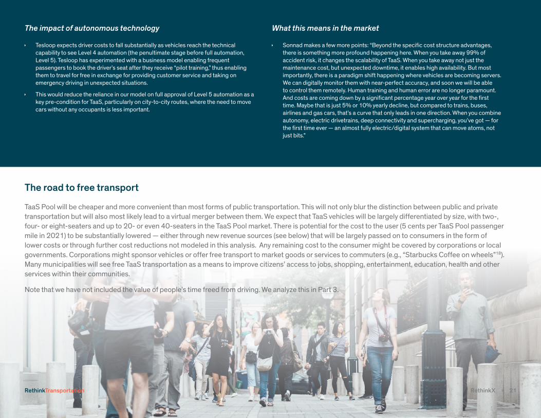
The road to free transport
TaaS Pool will be cheaper and more convenient than most forms of public transportation. This will not only blur the distinction between public and private transportation but will also most likely lead to a virtual merger between them. We expect that TaaS vehicles will be largely differentiated by size, with two-, four- or eight-seaters and up to 20- or even 40-seaters in the TaaS Pool market. There is potential for the cost to the user (5 cents per TaaS Pool passenger mile in 2021) to be substantially lowered — either through new revenue sources (see below) that will be largely passed on to consumers in the form of lower costs or through further cost reductions not modeled in this analysis. Any remaining cost to the consumer might be covered by corporations or local governments. Corporations might sponsor vehicles or offer free transport to market goods or services to commuters (e.g., “Starbucks Coffee on wheels”18). Many municipalities will see free TaaS transportation as a means to improve citizens’ access to jobs, shopping, entertainment, education, health and other services within their communities.
Note that we have not included the value of people’s time freed from driving. We analyze this in Part 3.
The impact of autonomous technology
ê Tesloop expects driver costs to fall substantially as vehicles reach the technical capability to see Level 4 automation (the penultimate stage before full automation, Level 5). Tesloop has experimented with a business model enabling frequent passengers to book the driver’s seat after they receive “pilot training,” thus enabling them to travel for free in exchange for providing customer service and taking on emergency driving in unexpected situations.
ê This would reduce the reliance in our model on full approval of Level 5 automation as a key pre-condition for TaaS, particularly on city-to-city routes, where the need to move cars without any occupants is less important.
What this means in the market
ê Sonnad makes a few more points: “Beyond the specific cost structure advantages, there is something more profound happening here. When you take away 99% of accident risk, it changes the scalability of TaaS. When you take away not just the maintenance cost, but unexpected downtime, it enables high availability. But most importantly, there is a paradigm shift happening where vehicles are becoming servers. We can digitally monitor them with near-perfect accuracy, and soon we will be able to control them remotely. Human training and human error are no longer paramount. And costs are coming down by a significant percentage year over year for the first time. Maybe that is just 5% or 10% yearly decline, but compared to trains, buses, airlines and gas cars, that’s a curve that only leads in one direction. When you combine autonomy, electric drivetrains, deep connectivity and supercharging, you’ve got — for the first time ever — an almost fully electric/digital system that can move atoms, not just bits.”
RethinkX » 21 RethinkTransportation

Box 6: Additional factors potentially driving TaaS prices lower
Other revenue sources. A-EVs could generate additional revenue streams, including from charges for entertainment, advertising, monetization of data, and sales of food and beverages. These would create more revenue for fleet owners, which in turn could be either used to reduce the cost of travel for consumers or retained as profit. As an example, advertising revenue based on 12 trillion passenger minutes in TaaS in 2030, with a captive audience and access to data about where they are going and who they are, could lead to highly targeted and valuable digital advertising space.
Grid back-up support. A-EVs could be used to provide back-up support for the U.S. and other national grids in times of peak demand. In our scenario, there will be 20 million TaaS vehicles in the U.S. in 2030, each with 60kWh batteries, resulting in a total of 1,200GWh of battery capacity. The peak draw on the US electricity grid changes between 475GW and 670GW in winter and summer, respectively.19 In times of peak electricity demand and low transport demand, A-EVs could be programmed to plug in and provide grid support.
Second life of batteries. Our analysis shows that after 500,000 miles, the batteries of A-EVs will still retain 80% of their capacity, which could be reused for grid storage. With 4 million A-EVs retiring annually, the surplus battery power could add 200 GWh of electricity storage to the grid each year.20 For comparison, the U.S. had 24.6 GW of energy storage in 2013.21
Efficiency gains in A-EV design and manufacture. TaaS fleet operators will be strongly incentivized by the potential size of their marketplace, which is likely to lead them to seek to achieve cost efficiencies throughout their supply chains. We therefore expect to see the prioritization of low-cost manufacture, ease of construction and maintenance in A-EVs.
Cheaper manufacture, more miles per A-EV. Competition between A-EV manufacturers may lead to lower upfront costs for TaaS fleet operators, through common modularized vehicle architectures and lower depreciation costs. A-EVs may have lifetimes greater than 500,000 miles as a result of ongoing innovation in autonomous technology, also leading to lower cost-per-mile.
Reduced maintenance costs. To outcompete other operators, there will be market incentives to drive down the costs of maintenance. Cost reduction can be made through the modularization of assembly and replacement parts, and through the automation of maintenance to save labor costs. Consumables will be designed for durability and lifetime, not for planned obsolescence.
Vehicle differentiation. The drive to lower production costs will lead to a standard hardware platform (consisting of the vehicle powertrain platform plus the vehicle operating system computing platform). However, this standard hardware configuration will allow manufacturers to offer a limitless variation in shape, type and performance from three-wheelers to performance cars to trucks and buses.
Cost savings relating to safety factors. As autonomous vehicles gain a bigger market share and safety improves dramatically, hardware requirements that were engineered under the assumption that there would be millions of car crashes per year will be less important. Metal that was used to increase vehicles’ body strength and weight will be shed, resulting in lower manufacturing costs.
» 1.3 Systems Dynamics
Systems dynamics drive adoption faster and further
In common with other technology-driven disruptions such as digital cameras, mobile phones and microwave ovens, the shift to TaaS will follow the technology-adoption lifecycle — that is, it will be non-linear, following an S-curve.22 The exponential nature of adoption is driven, in large part, by the effects of interacting systems dynamics, including a range of feedback loops, market forces and network effects. It cannot be assumed that technology costs drop and adoption increases while “all else remains equal,” as mainstream analyses do.
As adoption progresses, certain tipping points are reached where these dynamics affect the cost or utility of competing technologies, leading to an increasingly competitive TaaS marketplace. TaaS becomes progressively cheaper and improves its functionality, while ICE vehicles become ever more expensive to operate and harder to use. We describe below how some of these systems dynamics will operate over the adoption lifecycle.
A fast start in cities
At the outset of the disruption the policy, business and consumer drivers that we describe below will ensure that demand for TaaS exists, that a sufficient supply of vehicles is available, and that a supportive, enabling regulatory framework is created. Markets
RethinkX » 22 RethinkTransportationRethinkTransportation

will reward providers that supply vehicles with long lifetimes and low operating costs, which will both disrupt the basis of competition of the conventional car industry and trigger further cost savings.
TaaS adoption lifecycle reaches critical mass and tipping point
In cities where population density and real estate prices are high (e.g., New York, San Francisco, Boston, Singapore, London) TaaS adoption will likely proceed fastest. Pent-up demand from groups that are not served by the current IO market or have little or no disposable income will ensure that there are many early adopters of TaaS (the disabled, pensioners living on fixed incomes,23 millennials paying a large proportion of income on rent,24 middle-class families struggling to stay in cities25).
These users will build the critical mass for the TaaS market to reach a tipping point at about 10-20% of the passenger transport market. In line with the technology adoption lifecycle S-curve, once the market reaches this tipping point, demand accelerates, creating a virtuous cycle of more availability of TaaS vehicles, lower costs, higher quality of service, quicker pick-ups and faster rides. This will both increase usage from existing users (i.e., they will use it not only to go to work but also to go to the supermarket or pick up kids at school) and attract even more new users, further propelling the virtuous cycle.
Think of how the digital camera disrupted film cameras. The more early adopters used digital
cameras, the more services became available for digital imaging (Flickr, Shutterfly) and the cheaper digital cameras became, which attracted even more users and more ecosystem providers (Facebook, Instagram) which attracted still more mainstream users, and eventually even the more ardent lovers of film cameras put them aside for the vastly cheaper and superior functionality offered by digital imaging.
The flip side of the virtuous cycle of the disruptor is the vicious cycle of the disrupted. The IO ICE industry will enter a vicious cycle that includes plunging new car sales and used car values.
Vicious cycle making the demise of IO vehicles inevitable
As the early majority (mainstream market) adopts TaaS, the IO ICE industry will enter a vicious cycle that will disrupt the industry. Individual car owners will use their ICE vehicles less and less until they stop using them altogether. Early adopters who were car owners will sell their cars and not buy new ones. As TaaS penetration approaches the mainstream point (50%), a critical mass of users will stop using ICE cars, try to sell them and not consider buying a new one. Gas stations, repair shops and dealers will close, first in the cities and then in the suburbs. This will make it even more expensive and time-consuming for the remaining IO ICE drivers to have their cars fueled and serviced. The cost of operating IO ICE cars will keep rising, and the hassle of fueling them in gas stations farther and farther away from home will increase, while the cost of TaaS will drop
and its convenience increase. This will further widen the cost difference and convenience differential between TaaS and IO ICE, which will attract more users who will abandon their cars. More gas stations, repair shops, and dealers will shut down, further pushing the vicious cycle of the ICE industry. Spare parts will become more expensive and more difficult to source as suppliers shut down. Insurance costs for human drivers will rise as the data-driven insurance industry can price premiums according to actual driving patterns, making IO ICE even more expensive to operate. Speed of travel will pick up and congestion decrease because of TaaS, and soon it will become clear that humans are dangerous drivers and are slowing traffic down. Social pressure will lead to calls for legislation to limit areas or times where human drivers are allowed. Furthermore, demand for access to the benefits of TaaS from consumers in areas that are late in the adoption cycle will drive supply to expand and force regulators to consider universal-access measures. At this point, near total adoption of TaaS becomes inevitable as these systems dynamics ensure that IO vehicles are ever more expensive and difficult to operate, and the supply of TaaS reaches even the most rural communities.
Stakeholder dynamics
Disruption happens dynamically within the context of choices made by key stakeholders: consumers, businesses and policymakers. These groups are interdependent, and decisions by any group affect the decisions of the others.
RethinkX » 23 RethinkTransportation

Understanding the process of disruption requires insight into the likely behavior of these stakeholders. Below, we summarize our analysis of the key factors that will influence the behavior of each group.
Consumers will be motivated by cost above all else
Demand for TaaS, not supply, will be the key driver of disruption. The scale of the cost differential will override all other factors that influence consumer choice. Many of the perceived barriers to TaaS will be overcome as consumers are exposed to and experience A-EVs. Experimenting by taking a journey in a TaaS vehicle requires no investment other than downloading a phone application, and there are no penalties for taking one journey. The service can be tried at will and the option to cease to use TaaS is always available (it has high “trialability”26). TaaS and IO models are also not mutually exclusive; individual ownership and use of an ICE or EV can continue, alongside use of TaaS. Figure 4 summarizes the key factors that affect consumer choice.
The importance of other factors will vary by consumer, but in the face of 10-fold cost improvements leading to free or nearly free transportation, cost will be the overriding factor in consumer choice. Over time the reasons for initial resistance will diminish, and the appreciation of the economic gains and the improvement in lifestyle and other factors of consumer choice will increase, driven by systems dynamics which tilt the playing field ever further in favor of TaaS.
Business environment will favor low-cost TaaS
The sheer scale of the potential TaaS market (6 trillion passenger miles in 2030) and the competitive market dynamics will ensure that the supply of vehicles follows demand and that the price of TaaS trends toward cost.27 Businesses in this market are likely to face the following dynamics:
ê A winners-take-all marketplace is likely to emerge, driven by the platform network effects, as TaaS providers compete for the vast per-mile market (4 trillion US passenger miles at the TaaS disruption point, rising to 6 trillion 10 years out).
ê These effects are likely to lead to a market-share grab, as TaaS providers look to seize dominance of local markets by flooding the market with vehicles.
ê Cost per passenger mile will be a key metric, with market forces rewarding TaaS providers that drive this down (by lowering upfront costs and operating costs and extending vehicle lifetime miles). In fact, the current market incentives to manufacturers (selling car “units” and making money from repairs) reward the opposite model for lifetime and operating costs, and there are huge potential gains possible here as market forces change.
Figure 4. Summary of factors affecting consumer choice between TaaS and IO
RethinkX » 24 RethinkTransportation

ê Consumers will benefit from low per-mile prices in an intensely competitive marketplace, as prices trend toward cost, with any new income sources created likely to be passed on in the form of lower prices. It is likely that market forces will prevent monopoly pricing power even as oligopolies begin to form (see Box 7).
The existential threat that TaaS will pose to incumbent transport businesses should be a strong motivator for them to try to reinvent themselves, either as hardware (vehicle) manufacturers or as TaaS providers. The multi-trillion-dollar potential market opportunities in TaaS will also attract new entrants. In such a competitive market, it will initially be difficult for TaaS providers to secure monopolistic returns, and the consumer will benefit as any alternative sources of revenue are passed on. Competitive markets lead to prices trending toward cost. We expect highly competitive pricing, and perhaps even price wars and short-term loss-leader pricing as providers look to secure dominance in local markets. Over time, this dynamic will reverse, as winners begin to emerge and local markets become defined by the winners. We do not expect the winning platform providers to have the ability to impose monopoly pricing (see Box 7).
Box 7: Monopoly pricing?
Platform network effects: Pre-TaaS platforms such as Uber benefit from network effects. The more passengers the platform has, the more drivers it attracts, which leads to a virtuous cycle of shorter wait times and quicker rides for passengers, which leads to more passengers signing up, which leads to more drivers, and so on. The value of the platform increases with each additional driver and user. This two-sided network (drivers and passengers) forces a winner-take-all dynamic. In the end, there is only room for a small number of platforms in each geographic market. There are concerns that this dynamic will lead to a monopoly situation, with the winners able to charge monopoly prices to consumers and not pass on the cost savings. Our analysis suggests that this will not be the case in most markets.
The current Pre-TaaS platforms are two-sided markets. Drivers and users create network effects. The more drivers (cars), the more users, and vice versa. However, even now this network effect is mitigated by drivers working for multiple platforms (Lyft and Uber) at the same time, and by passengers having access to several apps.
Platform providers compete for a limited supply of drivers by offering incentives and charging a smaller platform fee. Uber has raised its platform fee, while Lyft has lowered it. Thus Lyft can attract more drivers and attempt to enable its own virtuous cycle.
The dynamics of Pre-TaaS favor a small number of providers in each geographic market (more mutually exclusive platforms means worse service and increased wait times). There is concern that these network effects will allow the “winners” to adopt monopoly prices as the market consolidates into a few providers. However, this dynamic does not translate into market pricing power. Each city is essentially its own local market, and any competitor (an investor, manufacturer or platform company) could purchase a local fleet and undercut the monopoly pricing. This dynamic would ensure that prices remain competitive and not monopoly-based.
The platform technology is based largely on software. This software will be developed by many companies seeking to win local markets — for instance, Didi in China, Uber and Lyft in the U.S., Ola in India, and Grab in Southeast Asia. The capability to use this software to enter new markets will be there and hence does not represent a barrier to entry. We would also expect a robust Android-like open source version to be available. In fact, Waze, a Google company, is offering a ride-hailing service that is competitive with Uber in several cities. LibreTaxi, a San Francisco-based startup, is offering free open source ride-hailing software. Anybody anywhere can download and use it for free and potentially become an instant competitor to existing market leaders like Uber.
The Pre-TaaS two-sided network effects will disappear once AVs are introduced, since no human drivers are needed. Barriers to entry into TaaS will thus fall, which will open up opportunities for new entrants. Both TaaS software and fleets of A-EVs will be readily available to enter new markets without the need to invest in recruiting drivers. This will prevent abusive market pricing behavior by the winning providers in most markets.
Platform providers will make money from volume, not margin. They will add new sources of revenues (for instance, vehicles might move goods when they are not moving people), new business-model innovations (for instance, charge video streaming services a fee to be an exclusive provider over the platform), and more product lines (drones as a service, perhaps) to increase the value of the network.
An analogy is Amazon Web Services (AWS), which is by far the largest cloud service provider in the world. It has consistently lowered prices in line with decreases in the cost of computing. It has not abused its market position even though thousands of companies depend on AWS for their information technology needs. Instead, AWS has expanded the range of products and services it offers, providing customers even more sources of revenues and value. The threat of deep-pocket technology competition from Microsoft, Google and IBM keeps Amazon from abusing its market position.
RethinkX » 25 RethinkTransportation

Policymakers can help accelerate or delay the transition to TaaS
Policymakers will face several critical junctures when their decisions will either help accelerate or delay the transition to TaaS. The first and most critical decision is whether to remove barriers at the national level, or by city or state. A national approach would be far faster. The U.S. government pledged $4 billion to accelerate the development of self-driving cars on a national basis.28 The National Highway Traffic Safety Administration (NHTSA) has already started developing a “framework for the safe and rapid deployment of these advanced technologies.”29
But California is not waiting for the federal government. The Golden State, home to many of the companies leading the AV disruption, such as Google, Tesla and Uber, has, at the time of publication, approved requests by 30 companies30 to test their self-driving cars on public roads and has proposed rules to allow fully autonomous (Level 5) vehicles as soon as this year.31
Many policymakers will be driven to act by the economic, social and environmental benefits of TaaS, including:
ê Technology leadership gains as countries, states, and cities vie to gain first-mover advantage in the development of technologies within the A-EV supply chain. Leadership here will ensure that businesses in these jurisdictions will be best placed to lead the disruption globally and capture the wealth and job creation associated with it.
ê Productivity gains from freeing up of time to work during commutes and faster transport times for consumers, leading to an increase in GDP of $500 billion to $2.5 trillion (see Part 3).
ê Consumer income gains, which we estimate as equivalent to a tax cut or income gain of $5,600 per household on average32 per year from 2021 or $1 trillion annually in total in 2030. Consumer spending is by far the largest driver of the economy, comprising about 71% of total GDP.33
ê Public sector budget gains from lower highway infrastructure costs and from the possibility of a “land bonanza” as publicly owned land within road right of ways is freed up for other uses.
ê Quality of life gains from improved mobility for those who are unable to drive themselves, access to transport for those who cannot afford it, cleaner air, fewer road fatalities and injuries, and the increased ability of governments to meet their climate change targets.
Policy might be driven at a federal level or state-by-state or city-by-city. Supportive federal policy would help to fast-track the transition; however, it is not a pre-condition. As some cities lead this process, the benefits of low-cost accessible transportation will become so evident that policymakers elsewhere will face business and societal pressure to fast-track the transition. We expect to see a competitive policy environment with countries and cities competing to lead the disruption, and thus capture the associated
benefits. Support could manifest in incubation for wide-scale pilots, accelerated approval of AV technology, investment in infrastructure, and introduction of clear and simple insurance rules that protect the public and clear legal hurdles holding up AVs.
Conversely, there might be hostility to the driverless TaaS disruption in some jurisdictions for cultural, socio-economic or political reasons, considering that incumbent businesses will suffer losses from the introduction of TaaS. For instance, up to 5 million jobs may be lost, leading to aggregate income losses of $200 billion per year. These losses can be offset both by job gains created elsewhere in the economy that will arise from increases in consumer disposable income and productivity and by job creation associated with global technology leadership. Resistance to TaaS will ensure these new jobs are created elsewhere in the world but will not avoid the job losses due to the disruption. Oil industry revenues will shrink dramatically. We therefore expect that the oil industry will lobby hard against regulatory approval of A-EVs. Those countries or regions that bow to this pressure will face a reduction in their competitive position globally, given the outsized benefits that a TaaS disruption will bring. The countries that dominated the late 20th century global economy (the United States, Japan and Germany) were some of the countries most poised to benefit from the ICE disruption of horse-based transportation earlier that century. Countries that fail to lead or make a transition to TaaS will become the 21st century equivalents of horse-based countries trying to compete with economies whose transportation systems are based on cars, trucks, tractors and airplanes.
RethinkX » 26 RethinkTransportation

All the technologies associated with TaaS are global. The TaaS disruption will be a global disruption. The technology adoption lifecycle suggests that there will be innovators, early adopters, mainstream adopters, late adopters and laggards. If one country, state or city bans or fail to approve AVs, the disruption will still happen, but in another country, state or city. Whatever barriers keep mainstream adopters from A-EVs will be erased as they witness the benefits that accrue to the early adopters. Similarly, the late adopters will follow closely behind the mainstream adopters. The only question about TaaS is who will be the innovators and who will be the laggards, not whether this disruption will happen.
Box 8: The mainstream view of disruption
Key arguments in mainstream analyses
ê Mainstream analyses predict that individual vehicle ownership will continue as the principal consumer choice — the business-to-consumer model. This is due to a number of reasons, including the belief that “we love our cars” (like we loved our horses), and the fact that these analyses do not perceive the extent of cost savings from switching to TaaS.
ê Most analyses see both EVs and AVs as one-to-one substitutions for ICE vehicles; that is, in the future, we will choose to own an EV or AV instead of an ICE.
ê Mainstream scenarios model autonomous technology as a feature, like rustproofing or alloy wheels, for individually owned cars. For instance, they envision an AV that would take a consultant from home to work, after which she would send her car back to park at home and wait to be called back to pick her up after work. This AV would still be parked 96% of the time.
ê EVs are seen as a disruption from above, with superior but more expensive EVs falling in price over time, leading to a shift from new ICE vehicle sales to new EV sales. Mainstream analyses envision the existing global fleet of a billion ICE cars would take decades to replace, with ICE sales continuing into the 2040s and beyond.34
ê Price comparisons between ICEs and EVs are mainly based on the traditional metrics of the conventional car industry, such as upfront costs of purchase (rather than cost-per-mile in TaaS). Vehicle lifetime has little impact on cost, as depreciation is based on residual value, not on lifetime miles.
ê Mainstream analyses generally see no mass stranding of existing vehicles.
ê As a result, mainstream forecasts show vehicle disruption as a multi-decadal progression, not as the sharp S-curve exponential shift that would happen quickly and change the business model of the entire industry altogether.
ê Mainstream analyses generally pay scant attention to the disruption systems dynamics that drive both the 10x cost differential between TaaS and IO ICE and the technology adoption S-curve that wipes out the existing industry.
» 1.4 The Speed and Extent of Adoption
Our model relies on regulation only insofar as it permits the use of Level 5 autonomous vehicles. Further supportive regulation can accelerate the speed of adoption that we model. We assume that adoption is driven by consumer demand, and that supply of TaaS anticipates or closely follows demand, given the size of the opportunity to businesses and the threat to businesses that fail to lead. The TaaS disruption point date of 2021 is a key variable, based on our assessment of technological readiness and regulatory dynamics. Given that key A-EV technologies are improving exponentially, the disruption point could happen sooner in some areas, in 2019 or 2020. The way that the adoption unfolds would not change from the assessment below. It would just happen sooner.
How adoption unfolds: Cities first, then radiating outwards
We see the adoption unfolding over five periods in the timeline:
PHASE 0: PRE-APPROVAL
This is happening today. In this period, Pre-TaaS (ride-hailing) companies gain critical masses of passengers and users in major cities around the world. While there is incumbent political opposition in some geographies, the idea of car-as-a-service becomes culturally
RethinkX » 27 RethinkTransportationRethinkTransportation

and politically acceptable, and it even becomes the norm in cities with high population density and high real estate prices. We will see the manufacture of vehicles with fully autonomous capabilities starting as soon as this year. The level of autonomy these vehicles use on the road will depend on regulation, not technological capability. These companies will collect data that will allow them to keep improving their self-driving technology and mapping capabilities on an exponential basis. Pilot projects testing fully autonomous technology increase from a few cities to dozens of cities around the world. Future TaaS providers develop their own self-driving car technology, license self-driving technologies from independent providers, or purchase self-driving technology companies and begin to build fleets in readiness for the disruption point. Legislation is introduced to abolish minimum parking requirements in new buildings in central business districts in cities around the world.
DISRUPTION POINT
This is the date when widespread approval of autonomous vehicle use on public roads is granted by regulators, which in our model we estimate as 2021.
PHASE 1: EARLY ADOPTION PHASE, YEARS 1-3.
Pre-TaaS companies convert their fleets to A-EVs and become TaaS providers. Urban users adopt TaaS for an increasing proportion of journeys. A-EVs become accepted by a growing number of mainstream users as exposure to them increases. In cities with the highest density
and real estate prices, TaaS quickly begins to provide more passenger miles than IO vehicles. Car owners stop buying new cars and begin to sell their vehicles. Legislation is introduced to ban ICE vehicles and non-autonomous vehicles in central business districts in cities around the world.
PHASE 2: MAINSTREAM ADOPTION PHASE, YEARS 3-8.
TaaS radiates outward beyond larger urban areas toward suburban areas, smaller cities and then rural regions. TaaS providers gradually merge, first in densely populated regions. Increasing numbers of users abandon car ownership altogether. Legislation to ban ICE and non-autonomous vehicles spreads to cities around the world.
PHASE 3: PLATEAU PHASE, YEARS 8-10.
The role of public transportation authorities will have changed dramatically, from owning and managing transportation assets to managing TaaS providers to ensure equitable, universal access to low-cost transportation. TaaS providers who may have lost the battle for the larger city markets expand into smaller cities and rural areas, filling in the remaining market gaps. Potentially, society will demand that public transportation authorities help provide TaaS availability for the full population, as has happened previously with the provision of telephony, water and electricity.
The speed and extent of adoption
Aggregating our analysis and applying our adoption framework, we conclude that:
ê TaaS will provide 95% of U.S. passenger miles within 10 years of the disruption point.
ê This 95% adoption plateau is based on 20-25% of rural users remaining non-adopters (see Box 9). Market penetration could rise above 95% if the vicious cycle of IO ICE markets lowers the quality and raises the cost of ownership to extreme levels, or if society requires that public transportation authorities provide universal high-quality TaaS service the way we have done in the past with telephone, water and electric services.
ê TaaS vehicles are almost 60% of those on roads in 2030. The 95% mileage figure equates to 60% of vehicles in the U.S. vehicle stock being A-EVs; the remaining 40% will be largely comprised of legacy individually owned ICEs. Our model sees 26 million TaaS vehicles and 18 million IO vehicles in 2030 (See Part 2).
ê Rebound in demand. Overall increase in passenger miles from 4 to 6 trillion. This increase is a function of: i) increases in travel by currently disadvantaged (often non-driving) users such as the elderly, disabled, poor, sick and young; ii) price elasticity and its consequences (lower prices trigger more demand); and iii) “slippage” from other
RethinkX » 28 RethinkTransportation

forms of transport such as short-haul aviation, buses and bicycles. It is likely that given the 10-fold decrease in cost, the addition of new demographics and the likelihood of free transportation, 6 trillion passenger miles is an underestimate. If so, this would point to a higher percentage of total miles being TaaS and a faster transition away from IO and ICE.
ê Urban TaaS will reach 95% market penetration sooner than the graph shows. Figure 5 shows adoption for the U.S. as a whole. Urban markets will move faster, and then TaaS will radiate outward to rural areas.
Box 9: The non-adopters
Who will be the 5% that do not adopt TaaS after 10 years? These non-adopters fall into three categories: rural consumers, the very rich and tech-laggards.
Rural consumers
We see this group as accounting for the vast majority of non-adopters. Smaller rural communities may not have the population density to have high enough demand to attract a critical mass of TaaS vehicles and maintain a sufficient level of service (in terms of waiting time, for example). This means that there will be many trips where the TaaS vehicle will have to wait for a passenger to take on a return trip or will make a long trip with an empty vehicle to pick up a passenger elsewhere. Waiting time and empty (“deadhead”) trips add to the cost-per-mile. There are several ways to ameliorate these issues. Planned trips can be scheduled in advance if a passenger can plan pick-up times (i.e., she works 9 a.m. to 5 p.m. and always has to be picked up at 8 a.m.). Predictive analytics by TaaS providers will become increasingly accurate in predicting when and where TaaS pickups will be required, which will dramatically diminish waiting times. Additionally, there is a credible counter-argument to rural consumers becoming late adopters. Rural populations are generally poorer than urban or suburban populations. The relative cost savings of shifting to TaaS will be far higher for rural families than for the rest of the population.
The very rich
This category is defined as those who are not motivated by road travel economics, despite the scale of the savings that TaaS offers. The closest proxy for this is the proportion of consumers who currently spend over five times the average price for a vehicle.35 The counter argument is that people with high paying jobs may have a bigger incentive to ride a driverless car because they will earn a lot more money by working in the car instead of driving. Either way, this group is small enough that is not material in terms of overall TaaS adoption.
Tech laggards
In this group, we place those who will not switch to TaaS for a range of personal reasons, including dislike of change, distrust of new technology and perceived loss of personal freedom.
It is possible that the feedback loops that will decimate the ICE value chain outlined above will make operating an ICE vehicle far too difficult and expensive, leading to a near-universal adoption of TaaS.
Vehicle supply will meet demand
Our analysis does not foresee supply side constraints affecting the delivery of the necessary vehicles to meet demand. The major risk to this statement lies in the potential bottlenecks in the supply of raw materials, particularly lithium and cobalt. Provided that the market anticipates the scale of disruption, market forces should deliver the required increases in supply of these materials. The increase in utilization of TaaS vehicles means that far fewer vehicles are needed to deliver the supply of passenger miles. Manufacturing or assembly constraints do not represent a barrier to our model. Furthermore, we do not see any other barriers causing this demand-led disruption to be derailed.
TaaS vehicles are essentially EVs with added information-technology hardware and software capabilities; thus, we use EV manufacturing capacity as the basis for our analysis. Assembly capacity, battery capacity and lithium supply are the factors frequently cited as potential supply constraints. Here we provide an outline of why we do not see these issues acting as brakes on the speed and extent of driverless TaaS adoption.
RethinkX » 29 RethinkTransportationRethinkTransportation

Assembly (vehicle manufacture) capacity. EV manufacturing capacity is growing, and our forecast is for capacity to far exceed the requirements that we model for TaaS. However, if the growth rate of new specialized EV manufacturing capacity drops dramatically, any assembly shortfall in capacity can be mitigated by conversion of ICE assembly capacity, which can easily be adjusted to produce EVs — which are far simpler to assemble. Companies such as Nissan manufacture EVs and ICE vehicles in the same plants. In fact, a significant portion of assembly happens on the same lines.
Battery manufacturing capacity. The ability to manufacture the required number of batteries is currently much debated. Factories to produce the batteries are under construction in the U.S. and elsewhere. These factories are relatively easy to scale, with most equipment available off the shelf, so this is unlikely to be a constraint. Discussions with multiple experts suggest that it takes just 9-12 months to build a new battery manufacturing plant able to produce multiple gigawatt-hours of battery capacity.36
Mineral supply for batteries. This is often seen as the potential key supply constraint, as the processes involved in opening a new lithium or cobalt mine and developing the attendant battery-grade refining capacity are complex and can take about three years. But our discussions with mineral experts suggest that the supply volumes required to meet the demand curves shown in our models are achievable. Current global lithium reserves exceed 30 million tons,37 and our estimates calculate that 1 million tons of lithium will be required, per year, by 2030.38 For analysis of cobalt supply for batteries, see Part 3.
Figure 5. The Speed of Adoption
Sources: Authors’ analysis based on U.S. Department of Transportation data
RethinkX » 30 RethinkTransportation

» Part 2: TaaS Disruption — Oil and Auto Value Chains
RethinkX » 31 RethinkTransportation

Summary
In Part 1, we touched on the likely impacts of the TaaS disruption on vehicle supply chains. This section explores the implications for the auto industry in more detail. We also analyze the disruptive effects of TaaS on the oil value chain.
Box 10: Value chain summary
Summary points:
The TaaS disruption, as described in Part 1, will have profound implications across the automotive and oil value chains. These include:
ê The number of passenger miles will increase from 4 trillion miles in 2015 to 6 trillion in 2030.
ê The cost of delivering these miles will drop from $1,481 billion in 2015 to $393 billion in 2030.
ê The size of the U.S. vehicle fleet will drop from 247 million in 2020 to 44 million in 2030.
ê Annual manufacturing of new cars will drop by 70% during the same period.
ê Annual manufacturing of new ICE mainstream cars sold to individuals will drop to zero. Car dealers will cease to exist.
ê Huge opportunities will emerge in vehicle operating systems, computing platforms and TaaS fleet platforms.
ê Global oil demand will drop from 100 million barrels per day in 2020 to around 70 million barrels per day in 2030.
ê The price of oil will drop to around $25 per barrel.
ê Oil prices might collapse as soon as 2021.
ê High-cost oil fields will be completely stranded.
ê Infrastructure dependent on high-cost oil fields, including the Keystone XL and Dakota Access pipelines, will be stranded.
» 2.1 Introduction
Our research and modeling indicate that the $10 trillion annual revenues in the existing vehicle and oil supply chains will shrink dramatically as a result of the TaaS disruption.39 As previous market disruptions have shown, the market valuation of companies serving these industries will shrink even more dramatically. There will also be new wealth and jobs generated by TaaS. As in previous disruptions,40 these gains may not accrue to today’s leading industry players.
In this section, we highlight key considerations that stakeholders may want to consider before the TaaS disruption reaches the point of no return.
Our findings point to nuance in the likely outcomes. Some parts of the vehicle value chain will face existential threats and are unlikely to survive; but other parts have the assets, capabilities, and technology to make a transition and even to achieve dominance within the new value chain that will be enabled by the TaaS disruption.
The outlook for the future of oil supply chains is universally bleak, with negative effects for all industry players. However, these negative effects will be disproportionally distributed across countries, companies and oil fields, depending on the cost of production.
Below, we look at the likely impacts of the TaaS disruption and examine the choices that auto manufacturers and oil companies will face. We provide a map of the supply chains (see Figure 6) for background.
RethinkX » 32 RethinkTransportation

Figure 6. Vehicle and Oil Supply Chains
» 2.2 Disruption of the Passenger Vehicle Value Chain
Disruptions, metrics and revenues
History demonstrates that disruptions bring new players — and new metrics.41 The disruption of road transportation will be no different. The principal metric of the conventional auto industry over the last century has been vehicle units sold;
how efficiently they were used was not a salient issue when assessing success.
The TaaS disruption will bring new metrics. Transportation companies that organize their resources around these key metrics will be best positioned for success, while those that ignore these new metrics will do so at their peril. From the date at which adoption of TaaS begins (the 2021 disruption point in our model), the key unit of measurement42 will be miles traveled, with four variants as the key indicators: passenger miles, vehicle miles, dollar cost-per-mile and dollar revenues per mile.
Revenues shrinking by two-thirds
We estimate that passenger miles will increase by 50%, from 4 trillion passenger miles in 2015 to 6 trillion passenger miles in 2030. However, the revenues generated will shrink significantly, from around $1.5 trillion in 2015 to $393 billion in 2030 — a decrease of more than 70% (see Figure 7).
RethinkX » 33 RethinkTransportation

Figure 7. Revenue distribution along the car value chain
Sources: Authors’ calculations based on data from Auto Rental, Edmunds, Kelley Blue Book, Ibis World, Statista, U.S. Bureau of Labor Statistics, U.S. Department of Energy, U.S. Energy Information Administration and the Wall Street Journal
Vehicle fleet size will drop by over 80%, from 247 million vehicles in 2020 to 44 million in 2030. The major driver of a smaller total vehicle stock is increased vehicle asset utilization (see Part I). Just 26 million vehicles will deliver the 5.7 trillion passenger miles traveled via TaaS in the U.S. in 2030, with the remaining 5% of miles attributed to 18 million legacy IO vehicles (see Figure 8).
97 million ICE vehicles43 will be left stranded in 2030, representing the surplus that will be in the vehicle stock as consumers move to TaaS. These vehicles may eventually become entirely unsellable as used IO vehicle supply soars and demand disappears (see Figure 8).
ê New vehicle annual unit sales drop 70% by 2030, from 18 million in 2020 to 5.6 million in 2030 (see Figure 9). While the number of vehicles in the overall stock drops by 80% over our timeframe, new vehicle sales suffer a slightly lower decline. This is because each vehicle under TaaS is travelling 10 times farther, and hence reaches its end of life more quickly. Vehicles in the TaaS fleet are therefore on a faster replacement cycle (in years) even though they have longer lifetimes (in miles).
ê New ICE vehicle sales44 are finished by 2024, just three years after the regulatory approval and commercial availability of A-EV technology. In 2024, the pre-existing vehicle stock can more than meet the passenger-mile requirement for transport under individual ownership.
RethinkX » 34 RethinkTransportation

ê Used ICE car prices plunge to zero45 or even negative value. The rising cost of maintenance, gasoline and insurance; the cost of storing or taxing worthless vehicles; and the lack of a used car market might mean that prices go to zero or even below. That is to say, owners may need to pay to dispose of their cars.
ê ICE vehicles eliminated from fleet by end of 2030s at the latest.46 Given that the average age of a vehicle on the road is 11.5 years47, we can expect that ICE cars sold before 2023 must be replaced by the mid-2030s. This means that the remaining ICE vehicles will be eliminated from the fleet before 2040.
ê Car dealers cease to exist by 2024, with no new IO car sales from 2024 onwards and no direct consumer purchases given that TaaS vehicles will be fleet owned.48
ê Car insurance will be disrupted49 by a 90% fall in the insurance costs incurred by TaaS users (relative to IO), which is driven by the elimination of theft and sharp reductions in insurer costs for liability, injury and vehicle damage.
ê Almost $50 billion in revenues from gasoline taxes will be lost in the U.S., with the shift from an IO ICE to a shared A-EV fleet.50 However, governments whose budgets depend on this revenue could shift to taxing miles rather than gasoline or diesel.
Areas of opportunity
While TaaS will trigger an enormous disruption, different industries along the vehicle value chain will be subject to disproportional losses and gains. While the commoditization of road passenger travel will drive down hardware margins and volumes, there will also be new opportunities, through the creation of higher-margin businesses in operating systems, TaaS platforms and services, and additional revenue streams, spurred by new business models built upon these platforms. These are outlined briefly, below.
Figure 8. Personal vehicle fleet size and composition between 2015 and 2030
Sources: Author’s calculations based on U.S. Department of Transportation data
Vehicle operating systems
The companies that develop A-EV operating systems stand to reap massive rewards, as has been the case for Microsoft, Apple, Google and Cisco through their development of computing, internet and smartphone operating systems.51
RethinkX » 35 RethinkTransportation

Currently, Tesla’s Autopilot is in a dominant position, having been tested for 1.3 billion miles;52 Tesla’s CEO, Elon Musk has stated that all Tesla vehicles will be fully autonomous by the end of 2017.53 Other early movers include Google (Waymo), NVIDIA, Uber and Baidu. Companies within the incumbent auto industry, such as GM and Ford, have also acquired Silicon Valley startups that are developing autonomous vehicle software.
Figure 9. Trends in vehicle sales
Sources: Authors’ calculations, U.S. Energy Information Administration (EIA) and U.S. Depart-ment of Transportation
TaaS platforms — a large and growing market opportunity
As with operating systems, TaaS platforms are expected to benefit from network effects: The more users a platform has, the more users it will attract. Once a TaaS platform reaches critical mass, it will become dominant in that market. Companies such as Uber, Lyft and Didi are examples of Pre-TaaS companies that have invested billions to win market share as they evolve toward the driverless A-EV disruption point.
The major difference between operating systems and TaaS platforms is that the network effects for the latter are local or regional. Being the market leader in New York or even in the U.S. does not necessarily translate into winning the same position elsewhere, such as in China or India, as has already been demonstrated in the competition between Uber and Didi in China. Similar dynamics seem to be playing out in India, where Ola is providing intense competition to Uber.
It seems clear that TaaS platforms will be the new transportation brands, as is already evident in the Pre-TaaS era of technology-enabled ride hailing, where consumer relationships are with Uber, Lyft, or Didi rather than with Toyota, General Motors or Volkswagen. The hardware portion of the road passenger transport value chain is thus likely to become commoditized, leading to manufacturer brand-value erosion. This would mirror consumer experience in most internet and social media contexts, where many user relationships are with Facebook, Google or Amazon, not the computer or networking companies which power their data centers.
Tesla’s recent announcement about the development of its own ride-sharing platform is an indicator of this future industry trend.54 Elsewhere, a number of platform-related developments by auto industry incumbents are in progress, including GM’s $500 million investment in Lyft,55 BMW’s ride-sharing service, ReachNow,56 and VW’s $300 million investment in Gett.57
A key outcome from the development of winning TaaS platforms will be the potential of data generated, to power new products and enhance services still further. The more miles traveled by a company’s vehicles, the greater the value of the data.58
RethinkX » 36 RethinkTransportation

Tesla’s Autopilot is an example where testing its software in real-life vehicles has generated data to improve its semi-autonomous capability. According to an NHTSA report, Tesla crash rates decreased by 40% after it introduced its Autopilot capability in 2015.59 Looking ahead, TaaS providers will use data derived from vehicle sensors to build mapping data, which could be used either to outcompete others directly, or as the basis of other revenue generation, such as licensing. And, at a more macro level, data from sensors could inform understanding and corresponding actions relating to weather, air quality, human foot traffic and even passenger health.
Computing platforms
Intel became one of the biggest market winners of the PC disruption by creating the central processing units (CPUs), which became the platforms for the two prevailing operating systems (MS-DOS and Windows). The TaaS disruption has also created a race to become the “Intel of autonomous vehicles.” For example, NVIDIA has invested heavily in repurposing its graphics processing units in order to run the deep learning software that is inherent to AVs. Intel itself recently spent $15 billion to acquire Mobileye, a self-driving technology company, to compete in this market.60
Entertainment, work and other opportunities
Americans spend around 140 billion hours in cars every year, a number that will increase by 2030.61 The TaaS disruption will free up time otherwise spent driving to engage in other activities: working, studying, leisure options and sleeping. This will act as an increase in productivity and provide a boost to GDP (see Part 3.5).
From the TaaS provider perspective, additional services could be offered, such as entertainment (movies, virtual reality), work services (offices on wheels) and food and beverage (Starbucks Coffee on wheels). Providers could act as distributors, earning revenues via a range of business models, including a percentage of sales generated on their platform (as in the Amazon and Apple stores), advertising revenues from onboard entertainment (similar to the Facebook and Google AdWords models), or the as-yet-undeveloped business innovations that are likely to arise from the TaaS disruption.
Implications for vehicle manufacturing companies
Margins in car manufacturing reduced
TaaS will pose formidable challenges for vehicle manufacturers. As consumers shift away from individual ownership, much lower retail ICE and EV unit sales will follow. In our modeling, margins will be reduced as the first mover’s advantage dynamics drives TaaS providers to price their services even lower, squeezing supplier margins,
and leading to a fall of 80% in manufacturing revenues by 2030 in our model. In parallel, we see further margin reductions from the commoditization of A-EV manufacture. Given these dynamics, value destruction is inevitable.
On commoditization, A-EVs have competitive advantages over ICEs because their powertrains have many fewer moving parts (20 versus 2,000).62 Further considerations relate to how parts are sourced and standardized. It is not a given that current car manufacturers are best equipped in these contexts. For example, batteries are often manufactured by specialized electronics companies such as Panasonic (battery provider to Volkswagen and Tesla) and Samsung SDI (which provides them for BMW.)63,64 It may be the case that original equipment manufacturer (OEM) companies will be akin to the electronic manufacturing services (EMS) providers in the communications industry (e.g., Foxconn’s role in the assembly of Apple iPhones). On standardization, the most likely pathway is for a base design that can be adapted to different vehicle sizes. Optional high margin extras such as rustproofing, extended warranties and paint proofing will become obsolete.
Taking these factors into account, we estimate an 8% manufacturing margin for OEMs. This may be conservative. If assembly moves closer to the electronic-products model, margins could be closer to 4%. Margins could fall further still if TaaS providers bypass vehicle OEMs and purchase directly from service companies, such as Magna, Continental and Delphi. This supplier bracket already produces most car components and even manufactures entire vehicles for OEMs today.
RethinkX » 37 RethinkTransportation

Brands
With the shift from individual to shared ownership, the passenger will have a primary relationship with the TaaS provider (who by default we see as the platform owner), not with the OEM. We therefore see the brand value in road passenger transportation residing with TaaS providers, not OEMs.
The future of incumbent car manufacturers
We expect to see four overall strategies available to car manufacturers:
ê Focus on hardware manufacturing and assembling. The TaaS vehicle assembly market will be a high-volume, low-margin business. As companies like NVIDIA and Google’s Waymo provide the computing platforms and vehicle operating systems for AVs, we would expect to see more companies entering the vehicle hardware market. Incumbent OEM manufacturers will be competing with existing automotive suppliers (e.g., Delphi, Continental, Magna) as well as new entrants including electronics assemblers (e.g., Foxconn), electric vehicle companies (e.g., BYD, NIO) and electric bus companies (e.g., Proterra). More companies will be competing for a market where fewer vehicles are needed.
ê Build and operate fleets for TaaS providers. This business model would require carmakers to not only manufacture vehicles
but also to operate and maintain them throughout their lifecycle. The emphasis of this business would be on providing vehicles at the lowest possible cost-per-mile for the longest possible lifetime. It would be a radical departure from the conventional OEM strategy of “pushing steel.” The new business model would reward companies that build vehicles with long lifetimes and the lowest possible lifetime cost of ownership. Making a transition to this dramatically different business model would then be a matter of cultural and organizational management.
ê Forward integrate to become a TaaS platform provider. The manufacturing and fleet operations businesses will be commodity businesses. The relationship with the passenger, as well as the brand value and profit potential, will shift to the TaaS platform provider. Companies like GM, BMW and Ford have started to realize this and have been investing in building capabilities to address these market opportunities. OEMs face a set of challenges because of a range of factors including: i) TaaS platforms require a particular skill set and culture and require the product-development speed of Silicon Valley high-tech software companies, not Detroit hardware companies; ii) the pressure to preserve OEM cash flows and sunk costs by pushing uncompetitive ICE vehicles; and iii) the likelihood that network effects will lead to the survival of a small number of platforms in any given geographical area.
ê Vertical Integration. Car manufacturers may aim to be vertically integrated providers
of A-EVs and TaaS service, participating in all parts of the value chain, including manufacturing, fleet operations, TaaS platform and vehicle operating system development. Some OEMs have invested in creating capabilities to make this possible. Ford and GM have acquired Silicon Valley self-driving technology companies, while Nissan has chosen to develop its own self-driving capability in-house.
Tactics that car manufacturers that survive are likely to employ in advance of the disruption point include:
ê Ramping up EV/AV vehicle manufacturing capacity before 2020 to ensure supply of vehicles is available in the early market-grab dynamic of the early TaaS rollout.
ê Acquiring companies building AV software.
ê Focusing on driving down vehicles’ cost-per-mile, lowering operating costs and increasing lifetime.
ê Stopping capital expenditures and R&D spending on individually owned vehicles and focusing on developing TaaS vehicles, including modularizing vehicle architecture, for ease of assembly, for different sizes of vehicle, and for ease of maintenance. Designing for high mileage utilization and end of life.
ê Partnering with or developing alternative revenue streams — such as advertising and entertainment — to help drive down net cost-per-mile.
RethinkX » 38 RethinkTransportation

ê Partnering with, acquiring or creating TaaS platforms.
ê Being at the forefront of AV trials and pilots globally.
ê When AVs are approved, flooding urban markets with vehicles to seize market share.
ê Leading the “roll-up” of local platform operators.
ê Using existing relationship with car owners to radiate outwards from urban centers to suburban and rural areas.
» 2.3 The Disruption of Oil
The TaaS disruption poses existential threats to the oil industry. Our findings indicate that global oil demand will peak around 2020 at about 100 million barrels per day, falling to about 70 mbpd by 2030 (see Figure 11). The effects of such a dramatic decrease will ripple through the whole value chain, causing systemic disruption from oil fields to pipelines to refineries.
We find that the implications of the TaaS disruption on the oil industry have not been fully recognized by the market. Current valuations of listed oil companies imply that stockholders are still basing their spreadsheet scenarios on the continuation of the individual ownership model, forecasting growth in revenues and cash flow for decades to come.
This section looks at the implications of the disruption of oil.
Rethinking oil demand under TaaS
Methodology
We modeled oil demand for the TaaS disruption, based on the following key assumptions:
ê U.S. passenger vehicle oil demand. We calculated the displaced oil demand from U.S. light-duty vehicle transport corresponding to the adoption rate forecast in Part 1.
ê Disruption of Trucking. We then included a 5% annual change in oil demand from 2021 from the disruption of medium and heavy-duty vehicles in the U.S.
ê Extrapolation of U.S. data globally. We then extrapolated these U.S. trends to Europe and China in the same year, and to the rest of the world with a four-year time lag, in order to approximate the disruption to global oil demand.
ê Business as usual (BAU) for remaining oil demand. For all other sources of oil demand in transport and other sectors, we assume BAU according to EIA forecast scenarios. We do not account for disruption to oil demand elsewhere in the transport sector, such as in aviation or shipping.
RethinkX » 39 RethinkTransportation

U.S. oil demand from passenger road transport drops by 90% by 2030
Using the EIA’s BAU forecasts as the baseline, the results of our analysis indicate that oil consumption from U.S. passenger vehicles will decline from over 8 million bpd in 2020 to under 1 million bpd in 2030. Over 7 million bpd of oil demand will be eliminated by the TaaS disruption. The implication is that around 90% of the U.S. passenger vehicle market demand for oil will evaporate within a decade.
Oil demand from trucking drops by 7 million bpd globally
Similar dynamics that enable the disruption of passenger vehicle transport also apply to the trucking industry, where we see A-EV trucks enabling a quick shift to TaaS.65
Labor and fuel are about 69% of operating costs of a truck in the U.S.66 and 71% in China.67 By replacing the human driver and bringing an order-of-magnitude decrease in the costs of maintenance and fuel, A-EV trucks will incur a substantially lower cost-per-mile. Companies in industries such as logistics that use fleets of trucks will face competitive pressure to lower the cost of shipping by moving to A-EV trucks. The trucking industry has already invested heavily to increase fleet asset utilization to about 50% today.68 A-EVs will likely increase this percentage. A key enabler will be the fact that autonomous trucks will have no regulatory restriction on the hours they can operate each day, unlike human truck drivers who are legally mandated not to exceed an hours-per-day limit. As with passenger vehicles, an increase in asset utilization triggers substantially lower costs-per-mile over the lifetime of the truck. As a result, company optimization of truck utilization will be critical for commercial survival.
Both incumbent and startup companies have already demonstrated autonomous truck technologies. For example, Daimler has been publicly driving its semi-autonomous truck in Nevada since 2015.69 However, disruptions usually come from outside the incumbent players. Otto, a startup company founded by an engineer who led the development of Google’s self-driving car (now Waymo), was acquired by Uber in 2016.70
We do not see range as a constraint in the disruption of ICE trucks. The U.S. Department of Transportation estimates that more than half the freight (by weight) in the U.S. is driven less than 100 miles, while 71% travels less than 250 miles.71, 72 These ranges are within current capabilities — and will continue to improve exponentially over the next decade.73
Medium- or heavy-duty vehicles account for 15% of petroleum consumption in the U.S.74 With a 50% decrease projected between 2020-2030, demand from the A-EV equivalents of these vehicles will decrease from 3 million bpd to less than 2 million bpd in the U.S., with global trucking demand for oil dropping by 5.6 million bpd against the EIA BAU forecasts.75
Figure 10. Oil demand in U.S. light-duty vehicle
Source: BAU based on EIA figures
RethinkX » 40 RethinkTransportation

Global oil demand peaks in 2020 at 100 million bpd and plunges to around 70 million bpd by 2030
For our global oil demand scenario, we applied the annual rate of change in light-, medium- and heavy-duty transport oil demand in the U.S. to the oil demand forecasts in China and Europe in the same year, and to the rest of the world with a four-year delay. Figure 11 shows the outcome of this analysis: global oil demand will drop from 100 million bpd in 2020 to 70 million bpd in 2030. That is, total global oil demand will decrease by about 30% in a decade.
Implications for oil producers
We predict three key components of disruption along the oil value chain:
ê Price collapse. Low oil prices of $25.4 per barrel (bbl) by 2030 will affect the entire supply chain, but most importantly will drive out expensive producers from the upstream sector. Infrastructure built to service high-cost specific fields will also bear the brunt of lower revenue from oil production.
ê Volume collapse. The impact of lower oil demand will be disproportional along the oil supply chain. Certain high-cost countries, companies, and fields will see their oil production entirely wiped out in this demand scenario.
ê Composition disruption. The dramatic changes in the composition of the demand for refined petroleum products will be another disruptive factor in the oil supply chain. On average, a U.S. refinery produces 19 gallons of gasoline, 10 to 12 gallons of diesel and 4 gallons of jet fuel from each 42 gallon barrel.76, 77 That is, about 69% of each oil barrel goes to gasoline and diesel. As 30 million barrels per day of gasoline and diesel demand are removed from global markets, the effect on crude oil production might be more profound and disproportional along the oil value chain. This is because oil markets are complex and simple averages do not necessarily apply. There are more than 150 different types of oil crudes processed by more than 600 refineries around the world.78 These refineries vary widely in their complexity and ability to adapt to shifting changes in oil supply and fuel demand composition. As demand for gasoline and diesel drops many refineries will not be able to adapt to new market conditions
Figure 11. Global oil demand with TaaS disruption of transport
Source: Authors’ calculations using U.S. Energy Information Administration oil demand forecast as a baseline
RethinkX » 41 RethinkTransportation

Oil drops to $25 per barrel or below
Figure 12 shows the equilibrium cash cost81 of oil in 2030 based on our demand scenario, and analysis and data obtained from Rystad Energy. Assuming demand drops to 70 million bpd by 2030, the market would reach equilibrium at a cash cost of $25.4 /bbl.
Economics dictate that when oil demand drops to 70 million bpd in a competitive market, the 70 million cheapest barrels will be produced. In our model, those barrels that are more expensive than the 70-millionth-cheapest barrel to produce globally will be uncommercial and have no market value. The implication is that high-cost oil will be left in the ground, while the assets associated with extracting this type of oil and the infrastructure (pipelines, refineries) that depends on it will be stranded and valueless.
Short term volatility in oil prices
While it is not our purpose to forecast oil prices in this sector report, we can speculate on how the disruption of transportation might impact prices in the interim. Short-term, prior to oil demand peaking in 2020, it is possible that we will see high volatility and even spikes in oil prices. There is great uncertainty on how shorter-term pricing will play out, but if TaaS builds toward the disruption point in the coming years, and if companies and investors become aware of the momentum, then we might see investment in exploration, production, shipping, refineries and infrastructure begin to dry up. This could lead to bottlenecks in global oil markets that create short-term supply constraints and oil price spikes before the disruption gets underway. Another potential spike would be possible if oil producers collectively decide to maximize short-term cash flow in anticipation of the disruption. This would be possible by temporarily
by shifting production to other oil ‘by-products’ such as jet fuel, heating oil, asphalt, petrochemicals and kerosene. They will shut down or face massive investment needs to retrofit to new market realities. A new refinery might take 5-7 years to commission and cost $18 billion79 while retrofitting an existing refinery might take $3 billion dollars.80 This means that until the market stabilizes, the 30 mbpd drop in demand of gasoline and diesel (which represent 69% of the output of an oil barrel) may disrupt the value chains of up to 43 mbpd of oil production.
Figure 12. Cash cost of producing a barrel of oil in 2030
Source: Rystad Energy UCube
RethinkX » 42 RethinkTransportation

agreeing to withhold just about two million barrels per day from the market.82
During the oil crisis of 2014 and 2015, crude oil prices crashed from $115 a barrel in mid-2014 to less than $30 in the beginning of 2015. This happened when supply outstripped demand by two million bpd.83, 84, 85 Our oil scenario predicts a drop of 30 mbpd by 2030 (which is 40 mbpd below the BAU estimate).
It is also possible that in the short term, prices over-correct as some countries or companies continue to pump oil that is unprofitable in the
expectation of a recovery in demand or a future increase in price. National oil companies might continue to make uneconomic investments that in the short term depress prices below the cash cost.86
While price volatility will likely rule the short- and medium-term, we are more confident in the long-term implications for oil prices, with a longer-term reversion around the cost of the marginal barrel of oil.
Oil volume collapse
Impact on countries
Figure 13 shows the volume of oil that will be uncommercial under our transportation disruption model across the top 20 countries in the world in terms of potential oil production in 2030. U.S. producers will be hit the hardest by the volume effect, as almost 15 million bpd of US oil — or 58% — will become uncommercial to produce at $25.4 cash cost. Likewise, more than half of oil production in Canada, Brazil, Mexico, Angola and the U.K. will be stranded. In contrast, Persian Gulf countries will be barely affected by shrinking volumes, as 95% or more of the oil in these countries will remain commercially viable.87 Compared to today, global oil production will be more concentrated in Russia and the Gulf countries by 2030.
Our analysis indicates that countries will be affected disproportionately by the disruption of transportation. The magnitude of the impact on individual countries depends on three main factors:
ê Volume collapse — the proportion of oil stranded (Figure 13)
ê Price collapse — the impact of market price (Figure 12) on economically viable oil
ê The relative importance of oil to the economy (Figure 14)
Rent from oil production is less than 1% of GDP in the U.S., compared to around 40% in Saudi Arabia and Iraq, and around 20% in Iran, Qatar and the U.A.E.
Figure 13. Top 20 countries by potential 2030 oil production, split by commercial viability
Source: Rystad Energy UCube
RethinkX » 43 RethinkTransportation

Saudi Arabia, Russia, Iraq and other countries with low cash cost of production will maintain relatively high production levels, but nevertheless will suffer from low oil prices, which will drive down revenues and profit margins from oil. Given that rents from oil are high in these countries, the price collapse will have a significant impact on their government spending and economic growth. Thus, in one way or another, all these oil-producing countries will be heavily affected by the disruption.
Figure 14. Oil rent as a % of GDP
Source: World Bank World Development Indicators,88 accessed on 25/01/2017
Figure 15. Potential 2030 oil production for select top companies, split by commercial viability
Source: Rystad Energy UCube
Impact on individual oil companies: Large oil companies with high proportion of stranded assets
Our analysis indicates that oil companies will be affected disproportionately by the disruption of transportation. The magnitude of the impact on individual companies depends on two main factors: price and volume.
That is, while global oil demand is forecasted to drop by 30%, companies such as Saudi Aramco would see the rate of uncommercial assets in their portfolio rising to just 4%, and, for companies like Rosneft, approaching 10% (Figure 15).
The picture would be very different for major oil companies such as ExxonMobil, Shell and BP. Assuming that these companies continue to invest under BAU assumptions, they could see 40-50% of their assets become stranded. Furthermore, even the 50-60% of assets that are potentially commercial would still suffer from a market of persistently low prices, causing revenues and earnings to plummet disproportionately.
RethinkX » 44 RethinkTransportation

Impact on oil fields: High-cost oil fields will be stranded
The extent to which countries will be affected by the volume disruption depends on the type of oil fields they have. Persian Gulf countries such as Saudi Arabia, whose production mainly derives from low-cost conventional fields, would barely feel any impact in terms of decreased volume. Countries with a larger share of shale oil, oil sands and offshore oil will see a higher proportion of uncommercial oil. Under a mainstream business-as-usual scenario, shale oil and tight oil could potentially constitute over 70% of U.S. supply in 2030. However, under our transport disruption model, 65% of these barrels would not be commercially viable. Other areas facing large-scale volume disruption include offshore sites in the North Sea (U.K.), Nigeria and Norway; Venezuelan heavy crude oil; Canadian tar sands; and the U.S. shale sites.
Impact on infrastructure: Pipelines and refineries
Infrastructure associated with fields that are largely uncommercial will be heavily impacted. Some key insights include:
ê The Dakota Access Pipeline (DAPL) would be stranded,89 as 70% of potential Bakken shale oil becomes uncommercial, leading to excess pipeline capacity. Plans call for the DAPL — a 1,173-mile pipeline designed by Energy Transfer Partners — to carry 470,000 bpd a day.90 Under our model, existing pipeline capacity will be enough to serve Bakken, even without the DAPL.
ê The Keystone XL Pipeline would be stranded,91 as costly projects will be stranded in the Canadian tar sands. The Keystone XL is designed by TransCanada to carry Canadian tar sands to the Gulf of Mexico for processing at refineries there and export to the international oil markets.92 Under our model, both the Keystone XL Pipeline and oil sand refineries in Gulf of Mexico will be financially unviable.
ê Refineries associated with uncommercial fields would need expensive retrofitting or would be shut. Refineries are generally set up to process oil of a particular variety, and different types of crude require different processing methods. Those refineries associated with or located near fields that will become stranded will face severe difficulties, either being forced to close or requiring substantial re-engineering.93
Figure 16. Potential 2030 cumulative liquids production, split by supply segment and commerciality
Source: Rystad Energy UCube
RethinkX » 45 RethinkTransportation

Box 11: Oil field example
Case study: Bakken Oil Field
Approximately 70% of the potential 2030 production of Bakken shale oil would be stranded under a 70 million bpd demand assumption. Our findings suggest that Exxon Mobil and Apache’s Bakken fields will no longer be viable (Figure 17), whereas other larger producers such as Continental Resources and Statoil will see erosion of 60% and 25% of their assets, respectively.
Impacts elsewhere in the oil value chain
Specialist engineering/oil services companies
High-cost oil is generally harder to extract and requires more involvement from oil services companies94 with expertise and focus in this field.95 These companies might have a disproportionately large exposure to high-cost projects that will be stranded by the demand disruption.
Shipping industry
Oil shipping will certainly be impacted by the volume decline in oil production, and this will lead to an oversupply of tankers and a sharp fall in freight prices. In turn, this could trigger a decline in the demand for new oil tankers, leading to a negative ripple effect along the shipping-construction value chain.
What to expect from oil companies?
Oil companies, as well as companies throughout the oil supply chain, have little room to maneuver as oil demand drops, with few strategies open to them given the speed of the disruption.
The history of disruptions and the specific actions of oil companies suggest that self-disruption or a change of business focus will, in most cases, not be a realistic option. Financial strategy suggests that asset sales or the sale of the whole business would be the optimal way to realize value. Finding a buyer would, of course, get more difficult during a market downturn, just like selling a house after the real estate bubble had burst during the Great Recession.
Figure 17. Top 20 Bakken producers listed by potential 2030 oil production, split by commercial viability
Source: Rystad Energy UCube
RethinkX » 46 RethinkTransportationRethinkTransportation

When denial turns to acceptance, oil companies will attempt to maximize value in multiple ways. Our analysis suggests that we will see an increasing number of companies choosing the following options:
ê Selling high-cost assets. These assets might include oilfields, refineries, petrochemical units and pipelines. In response to a changing business landscape and low oil prices, Shell has already pledged to sell $30 billion of oil and gas assets between 2016 and 2018.96 In early 2017, the company disposed of half of its North Sea oil and gas assets, offshore gas fields in Thailand, and Canadian oil sands projects.97,98
ê Selling the company. It is possible that, before the markets appreciate the scale of disruption, some oil companies could sell themselves and so maximize value. For instance, Saudi Aramco may raise $100 billion and value the company at $2 trillion, which would make it the biggest IPO in history.99 Selling or listing a company to “take the money off the table” is a time-limited opportunity and would only help “universal holders” if the sale was to a private or government entity. Sale to another public company would still leave universal holders exposed to the business.
ê Split their businesses into oil-based assets and other assets (chemicals, plastics, gas) to protect the “good” business from the problems and liabilities in the “bad” business.100 This has already happened in the electric utility industry, as companies such as RWE and EON split into disrupted fossil and nuclear “bad companies” and “good” growth-oriented clean-energy companies.
ê If they find themselves unable to sell oil assets, then they will likely focus on maximizing cash flow by winding down the business. They will write off or write down high-cost assets, cut capital expenditure and overhead, and offload as many liabilities as possible, preferably to unsuspecting taxpayers (see below). Exxon conceded that it may have to write down as many as 4.6 billion barrels in North American reserves in what would be the “biggest accounting reserve revision” in its history.101
ê Fight through government action and regulatory capture. Focusing on policy, regulation and subsidy to slow down or create barriers to AV and EV technologies, the key enablers of TaaS. Look for the revolving door between governments and the oil industry to go into high gear. Additionally, the oil industry will invest in influencing the public opinion against the adoption of autonomous technologies. In an era of post-truth politics, we expect a steady stream of falsehoods, fake news, FUD (fear, uncertainty and doubt) news and pseudoscience, to be produced in an attempt to shape public perceptions of AV technologies.
Liabilities in wind-down scenario
Investors, employees and taxpayers should be aware of the potential pitfalls of this strategy, and will need to fully understand the potential liabilities of oil companies, including contingent liabilities in assessing value to be realized here. Value destruction can happen in advance of a collapse in volume. The coal sector has seen almost total market-value destruction as coal volumes peaked and dipped only slightly, an effect exacerbated by their liability profile.
Liabilities to be aware of include the potential claim on cash flows of:
ê Debt holders
ê Workers — pension liabilities, healthcare liabilities and redundancy costs
ê Guarantees to other group entities
ê Lease payment obligations
ê Take or pay obligations
ê Clean-up costs — decommissioning, removal and restoration of wells and other facilities
RethinkX » 47 RethinkTransportation

» Part 3: Implications. Planning for the Future of Transportation
RethinkX » 48 RethinkTransportation

Summary
In Part 3 we explore the social, economic, environmental and geopolitical implications of the TaaS disruption. We look at the likely impacts within road transport systems, signposting both the benefits and negative impacts for countries, businesses, consumers and communities.
Key findings
ê U.S. household disposable income boost. Savings to consumers from adoption of TaaS could increase aggregate U.S. household disposable income by $1 trillion annually by 2030.
ê Increased GDP. Due to productivity gains of $1 trillion.
ê Oil disruption. Lower volumes and prices of oil will have geopolitical implications for energy security, military spending and regional stability.
ê Environmental, health and social benefits. The new TaaS-based road passenger transport system will reduce CO2 emissions, lower air pollution, improve health, increase the efficiency of material use, significantly enhance mobility and significantly reduce social inequality due to lack of access to transportation.
ê CO2 emissions reductions. TaaS vehicles have an order-of-magnitude lower lifetime CO2 emissions as compared to IO ICEs.
ê Driving jobs. Will be lost as a result of TaaS, resulting in aggregate income losses of up to $200 billion.
ê New industry. The creation of the multi-trillion-dollar TaaS industry will create wealth comparable to or larger than that generated by the personal computer, internet or mobile telephony booms.
Policy recommendations
There are several policy pathways that can assist the development of TaaS in ways that optimize the benefits and mitigate the adverse consequences, including:
ê Permitting the testing and adoption of A-EVs.
ê Establishing industry standards for passenger-data ownership and privacy as well as vehicle network security.
ê Launching open-data initiatives to make municipal road and traffic information available to the public and entrepreneurs.
ê Encouraging open-access technology development ecosystems, whereby entrepreneurs worldwide can develop and access open-source software and hardware, open data, open mapping, open AI and open education to develop TaaS platforms, AVs and EVs. These initiatives can help lower barriers to developing TaaS products and entering the TaaS market. This can in turn keep larger TaaS providers from exerting monopoly pricing power and ensure that benefits from lower costs-per-mile are passed on to consumers in all markets.
ê Developing planning strategies for the reuse of unneeded transport infrastructure, parking lots and roadside parking spaces.
ê Easing regulatory frameworks for the conversion of unneeded commercial garages to social and productive uses such as affordable housing, co-working spaces, art studios, in-law units, student housing and walk-up spaces.
ê Anticipating and legislating mitigation of negative impacts, including providing social, financial and health care safety nets, as well as re-training programs for displaced workers including (but not limited to) drivers and workers in disrupted oil and ICE sectors.
ê Investing in public education campaigns to communicate the financial, social, health and environmental benefits of TaaS and to foster public acceptance and trust.
RethinkX » 49 RethinkTransportation

» 3.1 Introduction
TaaS is likely to trigger a global competition to lead the disruption of the road transport system. Even without TaaS, technology companies, battery manufacturers and other key players in the A-EV race are motivated by a range of economic and social incentives. Policymakers in the U.S. and elsewhere have already started to devise smart policies to facilitate the transition to new mobility systems.102
Understanding the potential impacts of commercialized A-EVs and the resulting adoption of TaaS on road transport and the broader economy, as well as its economic, environmental and social implications, is a critical precursor to the development of enabling legislation and mitigation policies.103 See Figure 18 for a summary of the main potential impacts of A-EVs and TaaS.
There are many broader potential implications of this disruption across society. In this section, we highlight the social and economic implications, the environmental implications and the geopolitical implications. We also consider the toolbox available to policymakers.
Choices for policymakers
Policymakers will face multiple moments when their decisions will either accelerate or slow down the transition to TaaS. They could either enable leadership of technology innovation and accelerate the speed of transition or resist the disruption and lock into a high-cost transport infrastructure.
ê Leaders of disruption will benefit from positive impacts of new transport systems, devise enabling legislation, plan for new infrastructure and mitigate the adverse impacts.
ê Resisters of disruption will treat potential negative impacts as reasons for opposing TaaS, continue investing in high-cost infrastructure, and lobby against adoption of A-EVs and TaaS.
Figure 18. Potential Impacts of TaaS
» 3.2 Social and Economic Implications
Total U.S. household disposable income could increase by $1 trillion annually by 2030
Accessing TaaS will have significant savings104 for U.S. households. Our model estimates that cost reductions in personal transport across the U.S. will increase household disposable income by over $1 trillion (see Figure 7). The average American family spends $9,000 of its income on road transport every year. Switching to TaaS would result in yearly savings of around $5,600 per household.
RethinkX » 50 RethinkTransportation

The disruption is likely to have large impacts on the broader economy. On one hand, the increase in households’ disposable income will boost spending, with positive impacts on job growth across the economy. On the other, TaaS will reduce the number of jobs in the disrupted sectors.
Time freed from driving could increase GDP by an additional $1 trillion dollars by 2030
Americans spend roughly 140 billion hours in vehicles every year. The average vehicle has 1.5 passengers, so the time spent driving is 87 billion hours. If Americans were freed from driving to work or study, they could increase U.S. GDP by $0.5 trillion to $2.3 trillion by 2030.105 For context, the U.S. had a GDP of $18.56 trillion in 2016. The GDP benefits would accrue to the U.S. as a whole, not just the transportation sector. This potential contribution to U.S. GDP would likely act as a spur for policymakers to support TaaS adoption. The key point is that TaaS has the potential to trigger a significant productivity gain. The calculations above are indicative; their value lies in signposting the self-evident productivity gains that TaaS could bring to the American economy.
Job losses from driving will reduce income by $200 billion, but new jobs will emerge
Driving jobs will be stranded by autonomous technologies. The U.S. auto industry employs
1.25 million directly and 7.25 million indirectly.106 Five million jobs nationwide could potentially be lost due to self-driving vehicles107 (including 3.5 million truck drivers108,109), equating to 3% of the U.S. workforce. At the same time, new jobs will emerge in a shared mobility transport system serviced by electric and self-driving vehicles.110 If we assume that a net 5 million driving jobs are lost at an annual average salary of $40,000,111 this would equate to a reduction in income nationally of $200 billion.
Policymakers will need to anticipate and mitigate the negative impacts of job losses, including providing social, financial and healthcare safety nets as well as re-training programs for displaced workers, including (but not limited to) drivers and workers in disrupted oil and ICE sectors. (This will be the subject of a future RethinkX paper).
Increases in mobility and accessibility
Mobility improvements
Providing mobility and accessibility for all is an important function of the transport system. The availability of on-demand door-to-door transport112 via TaaS vehicles will improve the mobility of those who are unable to drive and those who cannot currently afford to own cars, including populations living on fixed or highly variable incomes. This impact is particularly significant in the U.S., where a large share of the population relies on driving due to urban sprawl and the low density of public transport infrastructure.
Improved access to workplaces and public services
TaaS will have the benefits of better connectivity and reduced travel time compared to public transport,113 along with lower costs compared to driving private vehicles. In the U.S., where the average proximity of residents to the nearest public transport stop is lower than in Europe, TaaS will likely reduce travel times even more. Faster and cheaper commutes will help to ensure that access to job opportunities, health and education services are available to all.114
» 3.3 Environmental Implications
There will be positive local and global environmental benefits arising from TaaS, but there could also be negative outcomes. We highlight the key issues below.
CO2 emissions reductions from light-duty vehicles will fall by 90%
One of the primary environmental benefits of switching to an electric, autonomous and shared personal transport system is the reduction of CO2 emissions. The transport sector contributes 26% of CO2 emissions in the U.S.,115 of which two-thirds comes from light-duty vehicle fuel combustion.116, 117 The new transport system would support U.S. climate commitments. 118
RethinkX » 51 RethinkTransportation

Our model shows that the TaaS disruption would trigger a reduction of over 90% in CO2 emissions from light-duty vehicle road transportation in 2030, compared to BAU projections.119
Electricity demand in the U.S. will increase by 18% compared to BAU
Charging A-EVs will increase electricity demand. Our estimates show that the A-EV fleet required under TaaS will use 733 billion kWh of electricity per year in 2030. This represents an 18% increase in total electricity demand in the U.S. in 2030,120 compared to the business-as-usual projections of the U.S. EIA (see Figure 19). While A-EVs will account for a relatively small share of electricity demand in the U.S., three quarters of growth in electricity demand will come from the expanding A-EV fleet. It is important to note that the increase in demand (kWh) does not imply a need to increase the capacity (kW) of the existing infrastructure. This is because the existing power system is built for peak demand, not efficiency. By scheduling A-EV charging in off-peak periods, we believe that the existing infrastructure can absorb an 18% increase in demand without material investments in generation infrastructure.
Energy demand for transportation in the U.S. will decrease by 80% compared to BAU
The TaaS fleet would use 2.5 quadrillion BTUs as opposed to 12.9 quadrillion for the BAU case121 with an ICE fleet. That is, A-EVs will reduce road transportation energy demand by 80%. It is important to note that while electricity demand would increase by 18%, total energy demand will decrease by 80%. This is because A-EVs are far more energy efficient than ICE vehicles. The shift from ICE to A-EVs may represent the single largest reduction in CO2 emissions in the U.S. A parallel shift to a clean energy grid means that the U.S. will have an essentially emissions-free road transportation system by 2030.
Figure 19. A-EV as a share of total electricity demand in the U.S., kWh per year
Sources: Authors’ calculations based on U.S. Energy Information Administration data
Per-mile CO2 emissions from A-EV production are far lower than ICEs
There is a widespread myth that A-EVs will emit more greenhouse gases during production than ICEs. This is not the case when production emissions are applied on a per-mile basis, across vehicle lifetimes.
The emissions improvement factors for A-EVs are threefold: from production, from tailpipes and from vehicle lifecycle emissions, including those from recycling/disposal.
RethinkX » 52 RethinkTransportation

As noted above, A-EV tailpipe emissions are zero if batteries are powered from renewables. For lifecycles, the emissions savings are around 50%, as borne out in studies of EVs sold in 2015 in the US.122,123
In terms of production, A-EVs might appear to have a worse emissions profile: one study found that manufacturing an EV has 15-68% higher emissions than manufacturing an ICE vehicle, mostly due to emissions associated with the production of the lithium-ion battery.124 Other studies report similar findings. 125,126 However, the comparison is based on several assumptions that require scrutiny:
ê “Mileage for EVs and ICE will be equal.”127 This assumption does not hold if we compare an A-EV operating under TaaS and an ICE under IO, as an A-EV has a lifetime of 500,000 miles, which is two and a half times that of an ICE. When taking the difference in lifetime mileage into account, emissions from A-EV production are lower on a per-mile basis by 33-54%. By 2030, the lifetime of A-EVs will be one million miles, reducing the per-mile emissions from production even further.
ê “Energy and resources required to manufacture lithium-ion batteries will remain static.” This assumption does not consider the significant cost reductions in the manufacturing of lithium-ion batteries, which have fallen 16% per year during last two decades. Battery producers have been learning how to use fewer resources and less energy to produce a given unit (kWh) of energy storage. Therefore, the energy
footprint of the production of A-EV batteries has already improved and will likely continue to improve on an exponential basis.
ê “Manufacturers will use the same dirty energy inputs to build their batteries.” Tesla, which has built the world’s largest battery factory, at 35GWh, has announced that it will power its factory with 100% clean energy from solar and wind.128 So Tesla vehicles clearly don’t have the same carbon footprint as other EVs, like those from BYD, which are built using a majority-coal grid. Apple has pledged that all its supply chain will run on 100% renewable energy,129 and its data centers already run on 100% renewable energy. Should Apple enter the A-EV market, its electric cars would have a near-zero carbon footprint.
When taking all these factors into account, we expect the carbon footprint of TaaS A-EVs to be at least an order of magnitude lower than that of ICE vehicles on a per-mile basis — a number that will continue to improve in the foreseeable future.
The new transport system will improve local air quality and public health
A smaller fleet and more efficient driving due to the adoption of A-EVs will reduce congestion and local pollution from fuel combustion, while an electric fleet would eliminate pollution entirely. Air pollution from exhaust gases has detrimental impacts on human health, an effect that is especially severe in cities. Globally, around three million deaths are due to exposure to outdoor air pollution every year.130 In OECD countries,
outdoor air pollution causes $1.7 trillion annual economic cost from premature death131 and ill health, while in Europe the cost of premature deaths from air pollution is estimated to be more than 1% of GDP.132 Half of these losses are attributable to road transport.133 Thus, shifting to an A-EV fleet and reducing the number of cars on the road will improve citizens’ health and well-being.
The new transport system could save up to 1.2 million lives worldwide annually
In 2015, 1.25 million people died from road traffic accidents globally, according to the World Health Organization.134 Moreover, every year up to 50 million people suffer from non-fatal injuries, which impact quality of life and incur economic costs in the aftermath of a road traffic crash. Autonomous vehicles will be safer than human drivers, leading to a decrease in road traffic accidents.
Materials and resource use from vehicle manufacturing will decrease
Switching to A-EVs will have positive impacts on resource efficiency and material use. The three most salient factors are:
ê A reduction in material used in each vehicle. The EV powertrain has far fewer parts than the ICE powertrain: There only about 20 moving parts in the EV powertrain versus more than 2,000 in ICEs’.135
RethinkX » 53 RethinkTransportation

ê A reduction in materials used as a function of the fall in the number of new vehicles in the fleet.
ê A reduction in waste as the incentives for car manufacturer survival changes from unit sales to cost-per-mile. As explained above, survival of car manufacturers will depend on building cars with long lifetimes and low operating costs. This means that they will optimize for minimum waste of resources in building and operating vehicles, including designing vehicle platforms with parts that are interchangeable and recyclable.
Furthermore, as traffic accident rates start to go down materially, we can expect OEMs to use lighter materials, as excess material and features that are based on existing traffic accident rates become redundant (see Part 2).
» 3.4 Geopolitical Implications
Here, we analyze two key geopolitical implications: the impact of reduced oil demand and low oil prices on oil producers, regional stability and the energy security of the U.S.; and the geopolitics of lithium in an A-EV dominated world.
Geopolitics of oil Net oil exporters will be hit hardest by reduced demand and falling price
Declining oil demand and low prices will create political instabilities in parts of the world that are highly dependent on oil, leading to a shifting balance of power in world politics. Many oil fields will cease production as oil drops in price, while low prices will affect the revenue of countries that continue to produce. Oil-dependent countries will be impacted more than those with diversified economies and large financial reserves. Net importers will benefit from both lower cost imports and less dependence on oil exporters.
The net exporter countries that will potentially be most affected by the disruption include Venezuela, Nigeria, Saudi Arabia and Russia. During recent oil crises, Venezuela and Nigeria underwent significant social and economic stress due to their small financial safety nets.136 In contrast, the impact of low oil prices on Saudi Arabia’s GDP was mitigated by its sizable financial reserves, and Russia was also less impacted, despite budget cuts and deepening recession.
Oil-producing countries face increasing political instability
With a sustained oil market downturn, we foresee that some of these countries will face political instability due to growing debt, cuts in social welfare expenditures and increasing poverty and inequality.137 Destabilization is likely to be greatest in countries where the most severe oil industry declines are experienced.
Energy security will be a less critical factor in U.S. foreign policy
The TaaS disruption will wipe out more than 8 million barrels per day of U.S. oil demand by 2030. In 2015, the United States was a net importer of 4.7 million bpd (it imported 9.4 million bpd and exported 4.7 million bpd).138 Oil markets and value chains are global, which means that petroleum exporters may also import petroleum technologies, products and services. This means that there is no such thing as petroleum energy independence until oil demand is reduced to zero. However, while the United States will have a high proportion of stranded oil assets, the country will be mathematically independent of oil imports by 2030. Energy security will be a far less critical component of American foreign policy and military strategy. Political instabilities induced by the collapse of the oil industry may have serious geopolitical implications for the U.S. in the short term. However, the country’s foreign policy and military strategy may need to be crafted anew, within a context where U.S. energy security is not one of the country’s top strategic geopolitical issues.
Geopolitics of lithium Supply risks will need to be identified
Currently, EV production and design have certain key resource requirements, including lithium, nickel, cobalt and cadmium. Lithium-ion batteries are by far the most critical input in EVs. Considering booming demand for these materials for manufacturing EVs, identifying risks
RethinkX » 54 RethinkTransportation

and instabilities in material supply and mitigation strategies is critical to the future of the industry.
Lithium geopolitics is entirely different from oil geopolitics
Lithium is a material stock and, in the EV industry, is only required to build the battery, while oil is a fuel required to operate an ICE vehicle. Lithium scarcity would only affect new vehicle production. Not having lithium is like not having a new engine; the existing fleet can still operate for years. Oil is essential to operate the existing fleet; thus, oil is a far more critical part of the value chain. Without oil, the existing fleet stops operating almost immediately, as the oil shocks of 1973 and 1979 clearly showed. In the short term, the geopolitics of lithium supply is thus less critical, and not remotely analogous to oil supply.
Lithium-ion battery manufacturing has fewer supply constraints
Like oil reserves, lithium is highly concentrated in few countries.139, 140 Lithium production is also highly concentrated, with four major producers in control of 85% of supply (Sociedad Quimica y Minera de Chile, FMC Corp, Talison and Albemarle Corporation).141, 142
Contrary to what their name might imply, lithium-ion batteries only have 2% lithium by volume.143 The cost of lithium is not a material part of the cost of a lithium-ion battery: It’s about 4% (rising from 2% after recent price spikes in lithium).144 The cost of lithium-ion batteries has decreased by about 70% recently, even as the spot prices for lithium have more than doubled.145 Our research indicates that the mineral quantities
required for battery demand are achievable if there is sufficient advance planning.146 Lithium is constrained by the relatively long amount of time needed to open mines and build refinery capacity (3-5 years) rather than by any shortage of the raw material itself.
Lithium-ion batteries can be built with close substitute minerals
There are many types of lithium-ion batteries, using different minerals according to the specific needs of the product. Each type of battery uses different chemistries and materials to achieve different purposes. For instance, smartphone providers may design a battery for fast charging but short longevity, because the smartphone is expected to be replaced within two or three years. Stationary grid storage providers, which store electricity at a home, business or on the grid, may design lithium-ion batteries with longer cycle life (say, 20 or 30 years). A battery for a high-end car that needs “insane” acceleration would be designed for higher voltages, while a city bus that doesn’t need the acceleration might use a different chemistry.
Tesla cars use lithium-nickel-cobalt-aluminum-oxide (NCA) batteries, while BYD buses use lithium-iron-phosphate (LiFePO4 also known as LFP) batteries.147 BYD also uses LFP batteries to power its EVs and hybrid EVs. These vehicles don’t need the acceleration of a Tesla Model S, but BYD batteries’ warranties are for 30 years, while Tesla’s warranty is for eight years.
The main components in the most common form of lithium-ion battery, nickel-manganese-cobalt
(NMC), are not lithium but a range of materials including cobalt, manganese and aluminum.148 In 2015, 41% of the global cobalt demand came from the battery industry.149 Almost all (94%) of cobalt supply is a by-product of nickel or copper operations, which is principally concentrated in the Democratic Republic of the Congo, a high-conflict country, which accounts for 60% of global supply. New mines opening in the near future will add roughly 35% to the global capacity of 94k tons.150 Limited production and rising global demand for cobalt resulted in a 50% increase in cobalt prices in 2016.151 Globally, about 68% of lithium-ion batteries are made with cobalt, while 22% are LFP and 20% are LMO (lithium-manganese -oxide).152 The latter is mainly used in consumer devices. Cobalt supply risk can be mitigated either by changing the balance of cobalt in the cathode or through the use of lithium-iron-phosphate batteries,153 which do not require cobalt.
About 80% of China’s EV batteries are LFP.154 Tesla recently announced that the company will prioritize sourcing raw materials from North America for its Gigafactory in Nevada, as well as changing its battery chemistry to mitigate material supply risks.155
Lithium mineral supply risks can be mitigated through recycling
Lithium batteries from A-EV retirements can be recycled for new batteries and other secondary uses, such as storage for utilities, homes and businesses.156 Lithium batteries will still have 80% of their original capacity after retirement from road transport.157
RethinkX » 55 RethinkTransportation

» Appendix A, Appendix B and Endnotes
RethinkX » 56 RethinkTransportation

» Appendix A
Cost Methodology
Introduction
Cost will be the most important factor affecting economic choice. The scale of the cost differential will be the key determinant of consumers choosing TaaS over IO. This section sets out the basis of our assumptions.
Upfront cost analysis
To model upfront cost for new vehicles (see Figure 20), we use the following methodology:
ê Vehicle types. Our analysis is based on the largest selling vehicles in each of three categories: small, medium and luxury vehicles. For ICE vehicles these are the Honda Civic, Toyota Camry and Mercedes S-Class. For EVs we use the Nissan Leaf, Chevrolet Bolt and Tesla Model S. These vehicles act as the baselines for our analysis.
ê Adjustments. For EVs we assume that the vehicle will have a 250-mile range by 2020 by increasing the battery size of current vehicles (if required) and applying estimates of increasing battery power density. The other major adjustment we make for EVs is to apply a battery cost of $200/ kWh from 2017.
ê Cost forecasts. These vehicles become proxies for vehicles in that category. We break vehicles into their major constituent parts and apply cost curves to these until 2030. The cost analysis comes from industry data and discussions with experts.
Figure 20. Upfront cost comparison of electric and gasoline vehicles to 2030
Sources: Authors’ calculations, Edmunds, Tony Seba and U.S. Department of Energy
For A-EVs in the TaaS fleet, we apply a reduced manufacturing and distribution margin of 8%. This is to account for the commoditization of vehicle production (more akin to electronics assembly), lower brand value and a shorter distribution chain as fleet owners buy direct from OEMs (see Part 2 for further detail).158
RethinkX » 57 RethinkTransportation

Depreciation and finance costs
Depreciation for TaaS vehicles (all of which are A-EVs) is calculated as the upfront cost divided by lifetime mileage (see below for the basis of this calculation). The upfront cost element is covered in the note above and Figure 20; in this section, we look at vehicle lifetime. As we show, there are several key differences between TaaS and IO vehicle ownership that affect the treatment of depreciation, meaning that vehicle lifetime mileage is the critical factor.
Vehicle lifetime
The concept of vehicle lifetime is not black and white; a vehicle reaches the end of its life when it is uneconomic to continue to repair it, with timespans and mileages varying considerably. Longevity can be extended by the replacement of individual parts, but eventually these costs outweigh the costs of buying a new or used vehicle and cease to make economic sense.
Our analysis divides the critical elements of the A-EV four main categories: the drivetrain and battery, the body and interiors, consumables (such as brake pads), and power electronics and sensors.
Our research on these elements analyzed the potential vehicle lifetime and the implications for replacement cycles. All parts are seen as potentially replaceable at the disruption point, and replacement costs are included in our maintenance costs assumptions.
Lifetime analysis
In our analysis we find that the limiting factor is the vehicle battery; we model the end of vehicle life when its battery capacity declines to 80%159 and attribute no value to an A-EV beyond this point.
However, the write-off assumption is conservative on several fronts. Many parts of the vehicle will, in fact, still have value in other contexts, for example as spares for maintenance in other A-EVs. Additionally, there is likely to be a role for batteries as a component of grid storage,160 and, longer term, we expect batteries to become replaceable consumables,161 similar to brake pads.
Higher utilization helps lower cost because some aspects of vehicle degradation are related to time: More miles per period of time lowers the degradation rate of a vehicle and these components, including the battery and the body. The implication is that if still higher utilization (i.e. above 40%) is achieved, this may lower costs-per-mile further.
A key finding is that A-EVs will last for 500,000 miles by 2021. This is 2.5 times greater than our estimate for the lifetime miles of an ICE in the same year (200,000). Below, we explain the basis of this assumption.
Powertrain. It is important to note that an A-EV powertrain is much less complex than an ICE; it has 20 moving parts, rather than an ICE’s 2,000. Furthermore, it operates in a far more benign environment, in which there is less heat
and vibration and fewer touching parts. As a consequence, degradations in A-EVs are much lower, as degradation is mainly caused either by moving parts that touch and degrade each other or by parts that produce heat. The small number of parts also makes EV assembly simple and inexpensive, and they are much more easily replaced than in an ICE. Taken together, these factors make EV technology both intrinsically longer lasting and economically competitive.
Battery. There are numerous chemistries that can be used in lithium-ion batteries, all with different properties that make them more or less useful for different applications. Here we highlight three:
Nickel cobalt aluminum (NCA) or nickel manganese cobalt (NMC): This is the chemistry used by Tesla. It has high specific power, which allows for fast acceleration. High energy density allows for greater range per kg. But this is offset by a shorter lifetime in charge cycles.
Lithium iron phosphate: This is used is buses, trucks and some cars. It is slightly lower cost, and has a longer life in charge cycles. But it has less specific power — less of an ability to accelerate. It has less energy density and hence vehicles get less range per kg.
We assume that larger vehicles that service mainly the TaaS Pool market would be based on lithium iron phosphate or NCA/NMC batteries, and smaller vehicles will rely on NCA/ NMC, though developments in either technology might change the balance. Performance (acceleration) is not a key criterion in a TaaS fleet.
RethinkX » 58 RethinkTransportation

Batteries are degraded by both time and use. In a high-utilization fleet, we do not think that time will cause material degradation to batteries, and so this analysis concentrates on use. The use element of battery lifetime is measured in charge cycles.162
Real-life data gathered from 500 Tesla Model S owners who had driven a total of about 12 million miles showed battery degradation of only 5% after 50,000 miles and 8% after 100,000 miles.163 Tesloop, a California Pre-TaaS startup that uses Tesla Model S and Tesla Model X, has seen battery degradation of just 6% after 200,000 miles. CEO Elon Musk said that Tesla battery simulations showed a degradation of less than 20% after 500,000 miles.
We are confident that lithium iron phosphate batteries are currently capable of 2500-3000164 charge cycles before they are depleted,165 and certainly will be by 2021, which we use in our model.166, 167 With a range of 200 miles, this gives a lifetime of 500,000-600,000 miles. Our model assumes that this increases to 5,000 cycles by 2030, although this is likely conservative.168
NCA/NMC batteries are supposed to have shorter lives. However, data from the field suggests these batteries could last significantly longer than predicted.169 This is preliminary data and cannot be extrapolated from. Below we consider the sensitivity of our cost-per-mile model to battery lifetimes.
We consider 3 different scenarios to look at the sensitivity of our TaaS cost-per-mile figures to battery lifetime. Firstly, where battery life is 500k
miles, there would be no battery replacement needed. Secondly, where battery life is 300k miles, it would be replaced once, lifting the vehicle lifetime to 600k miles given that the battery is the limiting factor to lifetime in our model and other parts can last this long. Thirdly, where battery life is 200k miles, the battery would be replaced twice in a 600k-mile lifetime. For a 500k-mile and a 300k-mile battery life, there is no impact on cost-per-mile; the increase in vehicle life to 600k miles offsets the increase in battery costs. For the 200k-mile battery life, there would be an increase of 1 cent per vehicle mile for TaaS. We do not consider that this would materially alter our findings on the speed of adoption.
The battery cycle analysis is based on batteries with a 250-mile range with a depth of discharge of 80%.
Motor. Motors are not new technology, and we have evidence of motor life in other high-utilization environments. EV motors will cover at least 500,000 miles without (or with low) maintenance.170 Therefore, we do not see motors as a limiting factor within our model.
Vehicle body and interiors. The major impact on vehicle bodies is corrosion. The effects of corrosion are correlated more to time than to mileage, although the latter also plays a role. Environmental conditions also affect corrosion, but it is apparent from decades of ICE vehicle use that A-EV vehicle bodies will extend well beyond 5 years, and even to 9 years as modeled for 2030. The body will not be a limiting factor, with only minor replacements and maintenance
required. For interiors, we have looked at replacement cycles for planes, buses and trains as proxies, with only minor costs seen, which we capture in maintenance costs. Durability tests performed on current Proterra electric buses by the Exova Defiance Test Facility showed that after 750,000 miles, “no part of the bus body or other systems were compromised, including the chassis, battery packs and mounting, windows and doors.”171
Consumables. The repair or replacement of brakes, tires, lights, sensors and other consumables can be easily carried out and are taken into account in the maintenance cost category of our modeling. The current business model for IO vehicles has incentives that drive planned obsolescence and replacement; TaaS incentives will drive the opposite.
For example, the regenerative braking systems used in EV buses and trucks have led to much lower (or no) costs for brake maintenance, one of the most frequently replaced vehicle components within an ICE.172
Power electronics and computers. Computer lifecycles tend to be time-based rather than mileage-based and are assumed to be physically robust enough to last for our estimated 5 year/500,000 miles A-EV lifetime. Software is assumed to be kept current through over-the-air updates. This is a different approach from the standard 3-year computer replacement cycle used in depreciation calculations, which favor obsolescence and regular replacement.
RethinkX » 59 RethinkTransportation

Conclusion. Overall, we consider the 500,000-mile lifetime of the vehicle by 2021 to be conservative. Other than the battery, we expect all other parts to last well in excess of 500,000 miles. Our sensitivity analysis around battery lifetime suggests that battery replacement adds little or no cost to TaaS, given the increase in overall vehicle lifetime if the battery is replaced. We also assume that vehicle lifetime will improve at 8% per year, leading to a 1-million-mile lifetime by 2030.
Calculating depreciation
The fall in depreciation costs for an A-EV relative to ICE depreciation costs is the single biggest component of cost savings in the TaaS model when compared to the costs of a new IO ICE. Upfront costs will be recovered in a depreciation charge, part of the cost-per-mile to consumers. There are a number of reasons why the depreciation charge will be different from the treatment of upfront costs in the individual ownership (IO) model (see Box 12). TaaS providers will allocate the upfront cost of the vehicle equally over the lifetime miles of the vehicle.
The calculation will be:
Depreciation = Upfront cost ÷ Expected number of miles in vehicle lifetime
This is entirely different from how depreciation is calculated in the IO model, where depreciation is based on a residual value calculation, which takes the expected drop in value during the period of ownership into account (see Box 12). Given that very few new IO car buyers own a vehicle for its lifetime, lifetime miles play no role in the IO calculation.
Box 12: Calculating depreciation for ICEs and A-EVs
Depreciation of individually owned vehicles (including ICE, EV and AV)
IO vehicles are sold before the end of their economic life. The default assumption for a purchaser of a car is that the vehicle will be sold before the end of its economic life;173 few owners retain a vehicle for its full lifetime, and many vehicles are leased. We use the lease finance model as the basis for our depreciation analysis, with the standard 3-year lease period as the baseline.
Depreciation of an IO car is a function of the change of vehicle value during ownership. The assumption that ICEs will be sold before the end of their economic lives implies that at the point of sale a vehicle has residual value. Depreciation is therefore calculated as the loss in value while the vehicle is owned; that is, the difference between the value at the point of purchase and the residual value.
Vehicle lifetime miles are not used as the basis for IO depreciation. In the IO market, vehicle lifetime miles are not a consideration in cost of ownership. Lifetime miles are not used as the basis for the depreciation calculation; most individual purchasers (and lease finance companies) are primarily interested in how much a vehicle will decline in value over a given period.
Cost-per-mile for IO depreciation is calculated by the decline in value divided by miles driven in the ownership period (in our analysis this is 33,900 miles for a new car, depreciated over 3 years).
Long EV lifetime is not relevant in the IO market. The 500,000-mile lifetime of an A-EV or EV equates to 44 years in the IO market, by which time the vehicle is obsolete. This reinforces our assumption that lifetime miles are not pertinent to depreciation in the IO market.
Depreciation of A-EVs in TaaS fleets
TaaS providers will own an A-EV for its entire lifetime. If they sell them on to each other, the value will be based on the remaining lifetime miles.
Much higher utilization leads to shorter vehicle life in years. We estimate that A-EVs will travel their 500,000 miles in under 5 years.
For accounting purposes, A-EVs are assumed in our model to have no residual value after 5 years. The modeling conservatively assumes that after 5 years (and 500,000 miles) the vehicle will be written off, rather than the constituent parts being re-used.
These factors lead to TaaS depreciation being calculated over the vehicle lifetime on a per-mile basis. As no residual value is expected at the end of the 5-year A-EV lifetime (and no sale during lifetime is expected), then the IO depreciation methodology is not applicable. As a result, we see depreciation of the cost of a TaaS vehicle on a per-mile basis as the logical calculation.
Our assumption is that TaaS providers will attribute upfront cost to lifetime miles evenly.174 This leads to a huge reduction in the depreciation cost.
RethinkX » 60 RethinkTransportation

The cause for the low depreciation charge per mile in the TaaS model becomes clear: vehicle lifetime — in miles — becomes a key element in the calculation (see Box 12). This is where EV technology has a huge advantage over ICE, with 500,000 lifetime miles by 2021 versus 200,000 for ICEs. In fact, the long vehicle lifetime means that the depreciation cost changes little even if the upfront cost of vehicles improves at a slower rate than we forecast.
The implication for consumers using TaaS is that depreciation will be a small fraction of the cost (1/500,000th of the upfront cost-per-mile). We provide a detailed explanation of why per-mile depreciation costs are lower in TaaS, and why a change in accounting practice can be made, in Box 12.
Finance charges
Finance costs are related to time; higher utilization will see better capital efficiency and lower finance costs on a dollar-per-mile basis. A finance charge is based on an annual or monthly ownership period; because TaaS vehicles will cover 10 times the miles in any period, the cost-per-mile for finance is 10 times less. In our comparative analyses, we treat finance costs for individually owned ICEs generically, irrespective of whether the vehicle is leased or purchased for cash, on the basis that there is an opportunity cost of capital in a cash purchase.
Maintenance costs
Vehicle lifetime, upfront costs and maintenance costs are all closely related. For ICE vehicles there are trade-offs between them: If the product is built robustly, then it will last longer and have lower maintenance costs but the upfront cost will increase. ICEs also have a maintenance cost curve that increases over vehicle lifetime.
These dynamics are different for A-EVs. As discussed above, these vehicles have intrinsically longer lifetimes and lower maintenance costs. Based on our analysis of A-EV maintenance costs over their lifetime, we model costs at 20% of the equivalent ICE vehicle.175
This estimate is conservative. Propriety data from high-use bus and truck EVs suggests that on a bottom-up analysis of maintenance costs, a lower figure would be appropriate. Furthermore, “vehicle disruption” could bring down the maintenance costs by modularizing the construction of vehicles with replaceable parts and by eliminating labor costs through automation of the maintenance process. Additionally, consumables can be designed for A-EV lifetimes.
These are significantly different maintenance incentives for ICEs, where the dealership system is highly dependent on a revenue stream from after-sales servicing and maintenance. In contrast, the TaaS industry will use cost-per-mile as its key cost metric. The market will
reward companies that achieve the highest possible lifetime mileage at the lowest possible cost. Other companies will simply be unable to compete.
We use two treatments for maintenance in our cost-per-mile analysis for IO ICE vehicles (see Figure 2). For new cars, we take the average maintenance costs for the first 3 years of ownership (to mirror the depreciation treatment). For the existing vehicle stock, when we calculate the operating cost alone of a IO ICE vehicle in Figure 2, we take the lifetime maintenance cost over 200,000 miles and calculate a per-mile average.
Insurance
As in the rest of the TaaS value chain, the insurance market will move to a cost-per-mile basis rather than an annual premium. We estimate a 90% reduction for A-EVs, relative to driver-controlled ICEs. This is based on analysis of the two principal components of insurance costs: 1) theft and 2) liability, injury and vehicle damage.
Theft
Although it would be possible for hackers to remotely steer a vehicle away, the risk of theft by this means will be low. Given that A-EVs will have
RethinkX » 61 RethinkTransportation
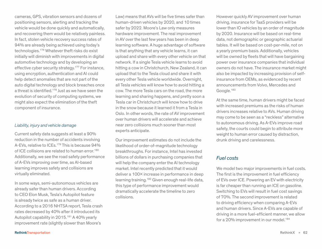
cameras, GPS, vibration sensors and dozens of positioning sensors, alerting and tracking the vehicle would be done quickly and automatically, and recovering them would be relatively painless. In fact, stolen vehicle recovery success rates of 94% are already being achieved using today’s technologies.176 Whatever theft risks do exist initially will diminish with improvements in digital automotive technology and by developing an effective cyber security strategy.177 For instance, using encryption, authentication and AI could help detect anomalies that are not part of the auto digital technology and block breaches once a threat is identified.178 Just as we have seen the evolution of security of computing systems, we might also expect the elimination of the theft component of insurance.
Liability, injury and vehicle damage
Current safety data suggests at least a 90% reduction in the number of accidents involving A-EVs, relative to ICEs.179 This is because 94% of ICE collisions are related to human error.180
Additionally, we see the road safety performance of A-EVs improving over time, as AI-based learning improves safety and collisions are virtually eliminated.
In some ways, semi-autonomous vehicles are already safer than human drivers. According to CEO Elon Musk, Tesla’s Autopilot feature is already twice as safe as a human driver. According to a 2016 NHTSA report, Tesla crash rates decreased by 40% after it introduced its Autopilot capability in 2015.181 A 40% yearly improvement rate (slightly slower than Moore’s
Law) means that AVs will be five times safer than human-driven vehicles by 2020, and 10 times safer by 2022. Moore’s Law only measures hardware improvement. The real improvement in AV over the last few years has been in deep learning software. A huge advantage of software is that anything that any vehicle learns, it can upload and share with every other vehicle on that network. If a single Tesla vehicle learns to avoid hitting a cow in Christchurch, New Zealand, it can upload that to the Tesla cloud and share it with every other Tesla vehicle worldwide. Overnight, all Tesla vehicles will know how to avoid hitting a cow. The more Tesla cars on the road, the more learning and sharing happens, and pretty soon a Tesla car in Christchurch will know how to drive in the snow because it learned it from a Tesla in Oslo. In other words, the rate of AV improvement over human drivers will accelerate and achieve near zero collisions much sooner than most experts anticipate.
Our improvement estimates do not include the likelihood of order-of-magnitude technology breakthroughs. For instance, Intel has invested billions of dollars in purchasing companies that will help the company enter the AI technology market. Intel recently predicted that it would deliver a 100x increase in performance in deep learning training.182 Given enough real-life data, this type of performance improvement would dramatically accelerate the timeline to zero collisions.
However quickly AV improvement over human driving, insurance for TaaS providers will be lower than IO vehicles by an order of magnitude by 2020. Insurance will be based on real-time data, not demographic or geographic actuarial tables. It will be based on cost-per-mile, not on a yearly premium basis. Additionally, vehicles will be owned by fleets that will have bargaining power over insurance companies that individual owners do not have. The insurance market might also be impacted by increasing provision of self-insurance from OEMs, as evidenced by recent announcements from Volvo, Mercedes and Google.183
At the same time, human drivers might be faced with increased premiums as the risks of human drivers increases relative to AVs. Human driving may come to be seen as a “reckless” alternative to autonomous driving. As A-EVs improve road safety, the courts could begin to attribute more weight to human error caused by distraction, drunk driving and carelessness.
Fuel costs
We model two major improvements in fuel costs. The first is the improvement in fuel efficiency of EVs over ICE. Powering an EV with electricity is far cheaper than running an ICE on gasoline. Switching to EVs will result in fuel cost savings of 70%. The second improvement is related to driving efficiency when comparing A-EVs and human drivers. Since A-EVs are capable of driving in a more fuel-efficient manner, we allow for a 20% improvement in our model.184
RethinkX » 62 RethinkTransportation

Platform and vehicle operating costs
These costs are treated in our modeling as a percent of the total per-mile cost associated with TaaS vehicle fleets. The cost of using a platform (the interface that connects the customer and the management of the A-EV fleet) is treated as 20% of the cost of a passenger mile.185 We include operating system costs in the upfront cost of the TaaS fleets, at $2500 in 2021. The competitive market environment of the early stages of the TaaS disruption will ensure that price trends toward cost. Given that both the operating system and the platform are essentially software based (with low marginal cost), we see little room in these markets for businesses to charge beyond this level.
» Appendix B
The Seba Technology Disruption Framework™
RethinkX uses the Seba Technology Disruption Framework™ to help analyze and model the disruptions in this study. Developed by Tony Seba, this framework is the result of more than a dozen years of research and teaching technology disruptions, business model innovation, finance, and strategic marketing of high-tech products and innovations at Stanford Continuing Studies, and has been used to understand and anticipate disruptions in several industries. The framework was the backbone of Seba’s 2014 book “Clean Disruption,” which has accurately predicted the ongoing disruption of energy and transportation due to technologies such as batteries, electric vehicles, self-driving vehicles and solar PV.
Here is a primer that summarizes the Seba Framework.
Disruption: A disruption happens when new products and services create a new market and, in the process, significantly weaken, transform or destroy existing product categories, markets or industries.
The digital camera disruption destroyed the film camera industry. However, disruption does not always imply the destruction of an existing market. For instance, the web significantly weakened but did not destroy the newspaper publishing industry. Ride hailing has radically transformed the taxi industry, but has not (yet) destroyed it.
Disruptions are made possible by the convergence of technologies and business-model innovations enabled by these technologies. Disruptions are also accelerated by open access technology development.
Convergence: Several technologies, each one improving at a different rate, converge at a certain point in time to make it possible for new products or services to be developed. Apple and Google launched the iPhone and
Figure 21. TaaS vs. new ICE: composition of differences in costs-per-mile
Source: Authors’ calculations
RethinkX » 63 RethinkTransportation

Android products within months of each other in 2007. That’s because the convergence of technologies that made the smartphone possible — in terms of bandwidth, digital imaging, touchscreen, computing, data storage, the cloud, lithium-ion batteries and sensors — all happened around 2007. By combining technology cost curves and business model innovations, the Seba Technology Disruption Framework can help anticipate when a given set of technologies will converge and create opportunities for entrepreneurs to create disruptive products and services. For example, Seba’s book “Clean Disruption” (2014) accurately predicted that the market would commercialize electric vehicles with 200-mile range at a cost of $35,000 to $40,000 (unsubsidized) by 2018. The GM Bolt and the Tesla Model 3 — leading a wave of such EVs — are now being pre-sold by the hundreds of thousands.
Technology cost curves: Technologies have cost-improvement curves, which show the rate at which a given technology improves over time. The best known technology cost curve is Moore’s Law, which postulates that computing power doubles every two years or so. The Seba Framework studies the economic side of these technology-improvement curves; that is, it looks at how a given unit improves on a per-dollar basis. For instance, when analyzing batteries, the metric we may look at is cost in dollars per kilowatt-hour.
For lithium-ion batteries, the cost per kilowatt-hour ($/kWh) improved at a 14% rate between 1995 and 2009.186 Technology cost curves improve due to a combination of factors,
including increased investments, research and development, manufacturing scale, experience and learning effects, openness, competition, standards, ecosystem integration, application across industries and the size of the market(s). Solar photovoltaic, when measured in dollars per watt ($/W) has improved from about $100 per watt in 1970 to about 33 cents per watt in 2017. This is an improvement rate of about 11.4% per year.
When we look at technology cost curves, it’s important to know what the main driver of the improvement is. Swanson’s Law postulates that solar PV costs tend to fall by about 20% for every doubling of cumulative shipped volume.187 Therefore, in the case of solar PV, the technology cost curve is mainly driven by volume, not time. Seba predicted in his 2009 book “Solar Trillions” that the cost of unsubsidized solar energy would be as low as 3.5 cents per kilowatt-hour by 2020, thus beating oil, coal, and nuclear. This prediction has recently come true.188 Demand for both coal and nuclear have peaked and declined, and market values of listed companies in both industries have collapsed as a result.
Exponential Technologies: Technology cost curves and their underlying performance improvement rates vary widely. Information and communication technologies have had high annual improvement rates (Moore’s Law has been around 41% per year), while solar PV technology has improved comparatively slowly (11.4% per year). The concept of exponential technologies, coined by Ray Kurzweil, refers to very fast technological change.189 While he didn’t draw a clear line as to what improvement
rate makes a technology exponential, his work has emphasized technologies that double their performance every year or two. Moore’s Law points to a doubling of computing performance every two years, while wireless communication was improving even faster, doubling performance every 10 to 11 months. The power of exponential technologies is that their performance vastly exceeds the human brain’s mostly linear comprehension of growth. For instance, Hendy’s Law postulated in 1998 that digital imaging had been improving at about 59% per year (measured as pixels per dollar). A 59% cost curve implies that the technology would improve by about 100 times in ten years, 10,000 times in twenty years, and 1 million times in thirty years. Steve Sasson invented the first digital camera in 1975.190 If Kodak had applied Hendy’s Law to Sasson’s invention, it would have predicted that in 2005 a $100 digital camera would perform at a level that would have cost $100 million to achieve in 1975. Kodak’s profits peaked in 1999, and the company went bankrupt in 2012.191 Both Hendy and Sasson worked at Kodak at the time of their discoveries. Other exponential technologies include sensors, artificial intelligence, 3D printing and DNA sequencing.
Technology cost curve improvement rates are not static. Sometimes they slow down temporarily or permanently. For instance, the internal combustion engine, which helped enable the car disruption of horse transportation a century ago, has not materially improved in decades. Small improvements in the cost-to-performance ratio of these technologies may
RethinkX » 64 RethinkTransportation

require massive investments. Technology cost curves can also accelerate. Batteries improved by 14% annually for about 15 years. This improvement enabled computer laptop computers, and later, smartphones. From 2010 to 2016, lithium-ion batteries improved by about 20% per year.192 As the cost per kilowatt-hour of lithium-ion decreases it helps to enable new markets, such as grid storage, residential electricity storage, unmanned aerial vehicles, and robots. The virtuous cycle continues to drive down costs where it can converge with other technologies to help enable disruptions of different markets at different points in the technology cost curve.
Disruption models
The Seba Technology Disruption Framework™ includes four key models that clarify how disruptions take place.
1. Disruption from below: (Clayton Christensen) A new product or service that is originally inferior compared to what the mainstream market offers improves its performance while decreasing costs at a faster rate than incumbent products.193 This faster rate of improve-ment is due to cost curves of the key technologies used to develop the product. This product may initially serve the needs of niche markets, and as it improves its utility, it expands into new markets. Eventually it overtakes and disrupts incumbent products and mar-kets. Examples include personal computers and solar power.
2. Disruption from above: (Tony Seba) A new product is superior but more expensive than competing products in the mainstream market. In time, however, the cost of the product is lowered until it becomes less expensive than incumbent products. By understanding the technology cost curves of the disrupting product, it is possible to predict when the disruption will take place. It is important to note that many times, these disruptive products are not just one-for-one substitutes, so analysts and industry experts don’t understand the coming disruption. The smartphone is a recent example. When the Apple iPhone came out at about $600 in 2007,194 experts said that it was not disruptive. Who would want to buy a $600 phone when they
could buy a $100 Nokia cell phone?195 What they did not understand is that a smartphone is not just a phone. An iPhone is a platform that allows us to do hundreds of things, including finding a date, getting driving directions, doing online banking, and, yes, making phone calls. The smartphone is not and never was a one-to-one substitute for the conventional cell phone. The electric vehicle (EV) is another example of a disruption from above. The EV is a superior product in a number of ways, not just an electric version of an ICE car.196 “Clean Disruption” lists nine reasons why the EV is disruptive. For instance, the battery in an EV allows us to power an average American home for a day or two (and up to two weeks in India).
3. Big bang disruption: (Larry Downes and Paul Nunes) A new product is better, faster, and cheaper than mainstream products on the day it is launched.197 Incumbent products have little or no time to react and are quickly disrupted. Examples include Google Maps with driving directions API, which disrupted the then growing GPS market served by companies like Tom Tom and Garmin. The Transportation as a Service (TaaS) disruption highlighted in this report is a Big Bang Disruption.
4. Architectural disruption: (Seba) A new product radically changes the way products and services are produced, managed, delivered, and sold. The architecture of the conventional electric power indus-try is centralized: it generates electricity with a small number of large power plants and delivers the electricity to millions of customers downstream in real time. Solar energy and batteries flip the archi-tecture of electricity: they enable millions of customers to generate, store, manage, and trade electricity. When the cost curves of solar and batteries (plus sensors, power electronics, software, and new business models) converge, the central generation model is disrupt-ed. At that point, the architecture of energy flips from central gener-ation to distributed generation. Architectural disruption is thus not just about technologies disrupting an existing market from below or above. Solar PV (plus storage) is disrupting every form of conven-tional power generation (coal, nuclear, natural gas, diesel). However, even solar (plus storage) generated in large power plants will not be
RethinkX » 65 RethinkTransportation

able to compete with on-site (rooftop) solar (plus storage). This is an archi-tectural disruption. The reason is that on-site generation and storage does not need the expensive transmission infra-structure needed to bring energy gener-ated at large-scale centralized plants to where the demand is.
Other models
Systemic disruption: Disruptions can potentially have devastating effects far beyond a single market category, causing whole sectors of the economy to be disrupted as a result. TaaS using on-demand, electric autonomous vehicles is not just disruptive to the ICE car manufacturing industry. It also has devastating effects on the oil industry as well as parking, insurance, car leasing and car dealerships. Like dominoes falling, it may also trigger dramatic impacts on shipping, logistics, real estate, and infrastructure, and the bond and equity markets. Tens of trillions of dollars (beyond vehicles) may be at stake because of the TaaS disruption.
Business model innovation: Business model innovation is every bit as disruptive as technology innovation. A business model includes the core logic and strategic choices for creating and capturing value within a value network.198 A business model innovation is a novel way of creating value and capturing value within a value network that is made possible by a technology convergence.
Disruptive business models may have a totally
new logic and new set of metrics that change the basis of competition, and make it extremely difficult (or even impossible) for incumbents to adapt or to win.
For example, ride-hailing (Uber, Lyft, Didi) is a business model innovation enabled by the convergence of smartphones and the Cloud. This convergence enabled instant connections and geographic matching between individual passengers and drivers with spare capacity in a highly efficient, convenient and cost-effective way. Ride-hailing (also called ride-sharing) companies applied a brokerage business model by taking a cut of every transaction.
Similarly, Airbnb is a business model disruption. Another example: the solar energy industry in U.S. residential and commercial markets grew exponentially after the introduction of a new business model called zero-money-down solar. In this model, the solar provider would finance, install and even own the solar panels. Traditionally, homeowners had to purchase the panels upfront. But the new business model allowed them to purchase or lease them like they did a car: with no or little money down, and agreeing to a set monthly payment for several years.
Note that the business models don’t have to be entirely new. Uber and Airbnb use the age-old brokerage business model, while solar borrowed the car lease and car loan models that have been used in the auto industry for a century. These business models were used in new settings to solve different problems, and were made possible by technology convergences.
Value network: Disruptors may leverage portions of existing value networks — a connected series of organizations, resources and knowledge streams involved in the creation and delivery of value to end customers — within and outside the industry they are disrupting, and/or create totally new networks that bypass the incumbents and reach customers in new ways. For instance, Tesla used the value network of the consumer electronics industry to source its batteries, hired people from the computer and auto industries, and created its own stores to reach customers directly, bypassing the auto industry’s dealer channel.
Metrics: Disruptive business models may create a totally new set of metrics that change the basis of competition and make it extremely difficult (or even impossible) for incumbents to adapt or to win. New industries create new metrics for success. Companies measure themselves and organize their resources around those metrics, and the market rewards companies that are best at optimizing those metrics. As an example, the music industry traditionally measured success as a function of album or CD units sold. These metrics dominated over other indicators (e.g., number of songs per album or number of times songs were played). Industry awards were created to reward those who maximized those metrics: Gold Records (500,000 sold) or Platinum Records (1 million sold) were designed to reward recording artists who maximized those metrics. The advent of Internet streaming (or music as a service) disrupted this metric, ushering in a new key metric: number of plays per song. This new metric changed the basis
RethinkX » 66 RethinkTransportation

of competition, bringing with it a totally new set of industry dynamics. Music-industry CD revenues plunged 84% in one decade, from $9.4 billion in 2006 to $1.5 billion in 2015, driven by on-demand streaming music.199 Streaming came “out of nowhere” to generate $2.4 billion. Streaming companies are software companies with zero marginal costs that generate revenues with a number of business models. By one measurement, it takes 1,500 streams to equal the revenues of one album sale.200 Traditional companies pushing CDs cannot possibly compete with streaming. Companies that organize themselves around pushing CDs cannot possibly compete in the new business environment. Similarly, Software as a Service (SaaS) companies (like Salesforce.com) ushered in new metrics that traditional software companies (like Oracle and SAP) could not compete with. They had to adapt or die.
Product innovation: Technology convergence makes it possible for companies to design products and services that solve customer problems in new ways. These products may have capabilities that create value in completely and heretofore unimaginable new ways, and they may make it impossible for incumbent products to compete.
The NEST Learning thermostat is an example. The convergence of sensors, mobile communications, computing, artificial intelligence, and the cloud made the product possible. The NEST learns users’ patterns and behaviors and adjusts temperatures automatically to match their comfort levels. To minimize energy usage, the thermostat adjusts
the temperature when the user leaves for work. An app that runs on smartphones makes it possible for the user to tell the thermostat to turn the heater or air conditioner on or off remotely. Using sensors, the NEST knows when a user is home, and uses artificial intelligence to adjust temperatures accordingly. It also has the capability to communicate with the utility to learn electricity prices, and to switch the heater and air conditioner on and off to save money while keeping temperatures within user comfort ranges. For instance, in the summer, it can “pre-cool” a home before the daily peak pricing period starts, and then turn the air conditioner on and off to maintain a comfortable temperature range while saving the owner money. Traditional thermostats could not possibly do this. Additionally, the thermostat communicates with the NEST Protect smoke and carbon monoxide detector. For example, upon learning from Protect that there is a carbon monoxide leak, the thermostat can shut down the furnace, a potential cause of the leak.201
Conceptual innovation: New concepts, methods, models, frameworks and software architectures enable totally new ways of doing things. Packet switching led to the development of the Internet Protocol Suite (commonly known as TCP/IP or Transmission Control Protocol / Internet Protocol), a new conceptual model of communications that led to the development of the internet.202 Blockchain is an open, shared, immutable, distributed ledger for recording the history of transactions (blocks).203 Like the internet, Blockchain is a conceptual innovation that can enable a wide range of new uses that
were not possible before. For instance, when Blockchain converges with technologies such as distributed solar PV, batteries, sensors, mobile communications and artificial intelligence, it could enable new forms of transactions between devices within the home and between neighbors, and cities — where the metric of value is a kilowatt-hour, rather than a dollar or a Euro – while bypassing the utility (or the government) as the centralized trusted payment intermediary. Conceptually, this could never have been done before, but now trust can be distributed and transaction sizes can be dramatically smaller and cheaper when using Blockchain.
Open access technology development (OATD): Open access allows knowledge, skills, data, technologies, inventions and products to be developed at an increasingly faster and potentially disruptive pace. Open access to capital enables entrepreneurs to create products that would otherwise not have been funded by traditional investors.
The following are dimensions of an open access technology development ecosystem that can contribute to the acceleration of disruptions:
ê Open data (Example: Climate.com)
ê Open content (Wikipedia, Safecast)
ê Open knowledge (Udacity, Coursera, Kahn)
ê Open-source software (Android, Linux)
ê Open-source development/collaboration (GitHub)
ê Open-crowd product development (Quirky)
RethinkX » 67 RethinkTransportation

ê Open innovation (Innocentive)
ê Open research (Materials Project)
ê Open business models (MySQL, RedHat)
ê Open APIs (Google Maps, OpenAI)
ê Open funding/crowd funding (Kickstarter, Indiegogo)
Open access lowers barriers to entry and lowers the cost and increases the speed of product development. It also reduces the ability of established companies to defend market positions, pricing power, and longevity of cash flows from existing products and services. Open access reduces advantages of scale, and reduces the need for corporations to build technology in-house. It allows anyone, anywhere to compete, leading to a dramatic increase in the number of competitors – and potential disruptors.
Silicon Valley is an example of an open access technology development ecosystem (OATDE) that combines the above dimensions within one geography. But the benefits and disruptive power of OATDE are spread around the world. For instance, the exponential growth in robotics development over the last decade has been enabled by an open-source operating system called ROS or Robot Operating System. ROS was initially developed at Stanford University and is now managed by the Open Source Robotics Foundation.204 Anybody anywhere around the world can download ROS for free and use it to create a new robot. Companies from MIT spinoff startup RethinkRobotics to French humanoid
robot developer Aldebaran have used ROS to develop robots for different uses and industries. If an engineer needs to learn artificial intelligence for robotics, she can go online to a website such as Udacity and take a free course offered by Georgia Tech.205 And while she’s at it, she can learn how to program a self-driving car, and maybe win $100,000 in the process.206 There are almost no barriers to a smart, committed engineer learning artificial intelligence and robotics to develop an autonomous vehicle. After doing that, it is possible to raise funds on a site like Kickstarter to take the product to the next level. If the entrepreneur wants to develop the whole vehicle, she can go to OSVehicle.com and use its open-source electric vehicle hardware platform.207 One hour of assembly required. A small team of engineers based purely on OATDE can disrupt a billion-dollar car company in Detroit, Toyoda, or Wolfsburg. This team can learn artificial intelligence for free, use free operating systems that they learned to program for free, access open-source electric vehicle hardware platforms, and raise money openly on a crowdfunding site.
Market and systems dynamics: Markets are complex adaptive systems. In complex systems, causal relationships are seldom (if ever) linear, and changes in single variables can trigger quick, exponential and massive effects. Technology markets are made even more complex as many technologies changing at different rates converge, enabling products and business models that were once impossible to develop or even conceive. Open technology development accelerates these converging interrelationships
even further. Additionally, technology markets have characteristics such as increasing returns, network effects, and adoption characteristics that enable disruptions to happen at increasingly faster rates and in ways that industrial-era resource-based industries cannot comprehend, let alone compete with. That’s because mainstream analysts tend to see markets as stable, linear, and relatively simple systems.
A reason for linear thinking is that the industrial era relied on supply-side economies of scale. Known simply as “economies of scale,” this norm posited that companies (and industries) gain cost advantage based on increased output, size, or scale of production.208 The larger you are, the more you produce, the less the unit of output costs. This in turn gives the company an advantage in the marketplace. Industrial-era businesses such as car companies, steel manufacturers, and conventional power-plant operators run by this principle: bigger is better.
Technology markets flip that equation because of information economics. Demand-side economies of scale are a function of the number of users, rather than the number of units of production. The more users a product or company has, the more utility it generates, both for other users and for the company that offers the product. Google search is an example: the more users use its search engine, the more data it generates, the more it learns, the more knowledge it generates, and the better its products get for all users, which leads more users to use it, and so on. That is, Google’s search engine exhibits increasing returns: each
RethinkX » 68 RethinkTransportation

additional unit of output is cheaper to produce than the previous one. Google’s value does not derive from the company’s massive data centers, but from the users of its search engine.
In his 2006 book “Winners Take All,” Seba described many characteristics of technology markets that created winners such as Apple, Google, Netflix, and Salesforce.com that have created platforms that exhibit increasing returns. There are no limits to the growth of knowledge, which makes these companies extremely valuable, especially when compared with traditional industrial and extractive industries. These four companies alone have created more than $1 trillion in wealth since Seba published “Winners Take All.” Not coincidentally, several of these companies are also developing some of the key technologies that are enabling the disruption of transportation described in this report.
Network effects: Demand-side economies of scale become powerful when users are inter-connected in networks. The value of the underlying network can grow exponentially with the number of users and connections that they have with one another. Think of the original telephone, or email network, or Facebook. If one person has a telephone or email or Facebook, it’s useless. When a second person joins the network, then you can connect with one person. Once a third user adopts, then each existing user can connect with two people. By the time a tenth user joins the network, each user can connect with nine other people, and the total combination of possible calls, emails, or connections is about
90. Once the millionth person joins, there are just under one trillion possible connections. Note two things: the first is that each time a new user adopts the technology, the value of the network increases for existing users. They get more value at no cost to them. Secondly, the value of the network increases exponentially; i.e., the formula is calculated to be around N^2 - N, where N is the number of users (this is called Metcalfe’s Law).
Network effects virtually guarantee winner-take-all markets. There’s no number-two network to Facebook. Operating systems like Microsoft Windows, Apple iOS, and Google Android have network effects. The value of the operating system increases with the number of users, which attracts software developers who create apps, which attract even more users, and so on, driving exponential growth in value. This virtuous cycle of value creation is the reason Apple, Google, Facebook and Microsoft have market valuations of hundreds of billions of dollars. In fact, these four companies plus Amazon are the five most valuable companies in the world, with a combined $2.6 trillion in market valuation (as of March 27, 2017).209
Technology adoption lifecycle S-curve: When Steve Jobs launched the Apple iPhone in 2007, mainstream experts and analysts from Bloomberg BusinessWeek to the Capital Group didn’t give it a chance. Bloomberg’s analyst wrote: “The iPhone’s impact will be minimal. It will only appeal to a few gadget freaks. Nokia and Motorola haven’t a care in the world.”210 Ten years later, there are 2.6 billion smartphones
globally.211 Whole industries have been launched because of the smartphone, and we could not imagine life without it.
Mainstream experts fail to appreciate that the technology adoption lifecycle is exponential, not linear. Adoption proceeds along an S-curve, where the early adopters who represent a small percent of the market set the stage for massive exponential growth as soon as the early mainstream users adopt a product or service.
Now that the smartphone has become a mainstream product, the expectation is that 6.1 billion users will have one by 2020.212 The total world population is expected to be 7.6 billion by 2020.213 That is, nearly every woman, man, and child on earth will use a smartphone just 13 years after its introduction. Not bad for a product whose impact was expected to be “minimal” by mainstream analysts.
S-curve acceleration: The adoption S-curve has accelerated over time. It took the telephone 75 years to reach 50 million users. Radio reached 50 million in about half the time: 38 years. The television did it in a third of the time it took the radio -- 13 years -- while the computer tablet reached 50 million in about a sixth of the time it took the radio: two years.214 The rate of acceleration has itself accelerated.
RethinkX » 69 RethinkTransportation

» Endnotes1 Challer, Bruce. 2017. Turns out, Uber is clogging the
streets. New York Daily News, February 27. Re-trieved from here.
2 Please see S-Curve graph in Seba Technology Dis-ruption Framework, page 12.
3 U.S. Bureau of Economic Analysis. Personal Con-sumption Expenditures and Gross Domestic Prod-uct. Retrieved from FRED, Federal Reserve Bank of St. Louis, here.
4 There are many potential new business opportuni-ties that might be unleashed by low cost transport. We use “Starbucks on wheels” as an example. If cost per passenger mile drops to 2-3c by 2030, the eco-nomics of running a Starbucks on wheels on popular routes might become hugely favorable compared to the cost of the real estate investment needed in city-center stores. If a 20-seater vehicle costing 2 cents per passenger mile covered 100,000 miles per year, the cost of the vehicle would be $40,000 per year, substantially less than the equivalent rent on a store. A Starbucks van could operate on popular routes, subsidizing travel costs through the sale of food and beverage. As autonomous technology begins processing costumer data sources, such as social media, marketing and e-commerce could also become potential venues for revenue generation.
5 Challer. 2017. Retrieved from here.
6 This is in line with announcements made by Ford, BMW, Toyota, Audi, and Nissan to launch self-driving cars by 2021 (Muoio, D. 2017. These 19 Companies Are Racing to Build Self-Driving Cars in The Next 5 Years. Business Insider UK, January 12. Retrieved from here). Other industry sources forecast an earlier date than 2021. For instance, Elon Musk announced that Tesla would produce a self-driving car that could travel between Los Angeles and New York by the end of 2017 (Stewart, J. 2016. Tesla’s Self-Driving Car Plan Seems Insane, But It Just Might Work. Wired, October 24. Retrieved from here). In
partnership with Lyft, GM will begin providing ride sharing services with thousands of self-driving Chevy Bolt electric vehicles in early 2018 (Fortune. 2017. GM and Lyft Plan to Deploy Thousands of Self-Driving Chevy Bolts. February 17. Retrieved from here). Rocky Mountain Institute estimates on-demand mobility services provided by autono-mous vehicles will be available by 2018 (Johnson, C. and Walker, J. 2016. Peak Car Ownership: Market Opportunity of Electric Automated Mobility Services. Rocky Mountain Institute. Retrieved from here).
7 This is based on our calculations for average house-hold expenditures on travel. American households own an average of 1.9 cars, and each car travels an average of 11,300 miles a year. In our model, the cost of travel by TaaS is 15.9 cents per vehicle mile, therefore average household expenditure comes down to $3,400. Source: US Bureau of Transport Statistics. 2001. National Household Travel Survey. Retrieved from here.
8 U.S. Bureau of Labor Statistics (BLS). 2015, U.S. average household spending on all except public transport in 2015. Consumer Expenditure Survey 2015. August. Retrieved from here.
9 The spike in IO ICE and EV costs between 2021-4 are related to the depreciation cost treatment. As TaaS becomes available and users begin to switch, there will be a surplus of used cars on the market, and a fall in demand for them. We see residual values for these vehicles dropping which affects the cost-per-mile,
10 These figures for cost in 2030 do not consider the diseconomies of scale or other negative feedback loops that might occur as new ICE sales decline and costs of ownership rise.
11 TaaS Pool figures are for cost per passenger mile; other costs are all cost per vehicle mile.
12 In this comparison, we adjust the A-ICE Platform cost to be the same as the A-EV cost as opposed to applying the same 20% of cost-per-mile charge, which would lead to a proportionately higher charge for the A-ICE platform.
13 Based on an interview with Rahul Sonnad, CEO Tesloop.
14 The battery of this Tesloop vehicle was replaced at 200,000 miles, but this was due to a software fault that affected the fuel gauge.
15 Tesloop charges its vehicles up to 5 times per day to 100% using superchargers. Although fast charging degrades the battery faster, the company made a strategic decision to move the vehicles with degrad-ed batteries to shorter trips. To date, Tesloop has not needed to put this strategy into practice.
16 At this level, Tesloop expects battery degradation of 30%. Our model assumes end of battery life at 20% degradation.
17 Tesloop also had some problems with lights due to high-water floods.
18 There are many potential new business opportuni-ties that might be unleashed by low cost transport. We use “Starbucks on wheels” as an example. If cost per passenger mile drops to 2-3c by 2030, the eco-nomics of running a ‘Starbucks on wheels’ on popu-lar routes might become hugely favorable compared to the cost of the real estate investment needed in city-center stores. If a 20-seater vehicle costing 2 cents per passenger mile covered 100,000 miles per year, the cost of the vehicle would be $40,000 per year, substantially less than the equivalent rent on a store. A Starbucks van could operate on popular routes, subsidizing travel costs through the sale of food and beverage. As autonomous technology begins processing costumer data sources, such as social media, marketing and e-commerce could also become potential venues for revenue generation.
RethinkX » 70 RethinkTransportation

19 The U.S. electricity demand data points refers to peak demand on February 3 and August 3 in 2016. US EIA. 2016. US Electricity Demand and Supply Balance. Retrieved on February 22, 2017 from here.
20 The calculation of 200GWh is simply 4 million batteries x 60kWh each x 80% (rounded). U.S. draws 640GW maximum and an average of 500GW. For eight-hour storage, you would need 8 x 500 = 4,000GWh.
21 U.S. Department of Energy. 2013. Grid Storage. December. Retrieved from here.
22 Seba, Tony. 2006. Winners Take All — The 9 Funda-mental Rules of High Tech Strategy. Amazon Digital Services LLC.
23 Pension Rights Center. Income of Today’s Older Adults. Retrieved from here.
24 Malito, Alessandra. 2017. Why American millennials may never get to live alone. Market Watch, March 19. Retrieved from here.
25 Boak, Josh. 2015. 1-in-4 US renters spend half their pay on rent and utilities. Associated Press, May 1. Retrieved from here.
26 Trialability is ease of testing or using a product or service. See Rogers, E. M. 2003. Diffusion of Innova-tions. New York: Free Press.
27 Peteraf, M. 1993. The Cornerstones of Competitive Advantage: A Resource-Based View. Strategic Man-agement Journal 14(3): 179-191.
28 Laing, Keith. 2016. Obama pledges nearly $4 billion for self-driving cars. The Hill, January 14. Retrieved from here.
29 National Highway Traffic Safety Administration. Automated Vehicles. Retrieved from here.
30 California Department of Motor Vehicles. Testing of Autonomous Vehicles. Accessed April 19, 2017. Retrieved from here.
31 Burgess, Matt. 2017. California could get truly driverless cars with new rules. Wired, March 13. Retrieved from here.
32 This assumes the comparison is with TaaS Private and not TaaS Pool. The figure of $1 trillion for 2030 is based on an even split of miles between TaaS Private and TaaS Pool.
33 U.S. Bureau of Economic Analysis, Personal Con-sumption Expenditures and Gross Domestic Prod-uct. Retrieved from FRED, Federal Reserve Bank of St. Louis, here.
34 Bloomberg New Energy Finance. 2016. Electric vehicles to be 35% of global new car sales by 2040. February 25. Retrieved from here.
35 The average price of a new car or truck sold in the U.S. in 2015 was $33,560. (Kelley Blue Book. 2016. Retrieved from here).
36 Lead times on opening battery factories is short, with most estimates we have received from experts being under 1 year for the opening of Giga-scale factories. The major constraint on battery factories is material supply. Tony Seba and Simon Moores, Benchmark Minerals.
37 U.S. Geological Survey 2017. Lithium. Retrieved from here.
38 Lithium is a relatively abundant resource, found in many parts of the world. The countries with the largest reserves are currently focused in Bolivia and Chile. But it is found also in Canada, Russia, China, and parts of Africa (U.S. Geological Survey, 2017). Under our TaaS scenario, global TaaS vehicle production would be 28 million by 2030. By 2030, batteries will require 0.6kg of Lithium per kWh — an improvement from 0.8kg currently (Interview with Simon Moores, Benchmark Minerals, January 2017). The average battery size is 60 kWh in our model, meaning each car would need 36kg of Lithium. Annual lithium requirements would be 1 million tons per year (assuming no recycling). Current global identified resources are over 40m tons, though we expect market forces to drive more to be discovered
and added to reserves as production increases. Even with an increase in rebound effect as transport becomes rapidly more affordable in developing countries, given the timescales involved, we would expect lithium supply to be able to match demand. Lithium demand in our model is within the constraint identified by our experts.
39 The Economist. 2016. Uberworld. September 3. Retrieved from here.
40 As an example, a large percentage of the revenues and profits in newspaper publishing shrunk dramati-cally in the decade after Google created AdWords (in 2000), while trillions in new wealth was created by online news-providing companies including Alpha-bet (Google), Facebook and Baidu.
41 As an example, the music industry traditionally mea-sured success as a function of album or CD units sold. These metrics dominated over other indicators (e.g., number of songs per album/CD, number of times songs were played). The advent of internet streaming (or music as a service) disrupted the metric (to number of plays per song) as well as music industry dynamics, business innovation and revenue models.
42 These changes in metrics also act as pointers to the underlying dynamics of the disruption, which will be characterized by a new focus on asset (vehicle) efficiency, business model innovation (the rise of platform-based TaaS providers) and new reve-nue streams (the new customer-facing per-mile charges).
43 The 97 million IO vehicles represent the surplus of passenger miles in the IO vehicle stock divided by 11,300 (the average current vehicle miles per year). It is possible that not all these vehicles will be stranded, and the “surplus” miles that the IO stock has available is met by more vehicles doing less than 11,300 miles, and thus more vehicles are partially stranded.
RethinkX » 71 RethinkTransportation

44 As new car sales for any given year are defined as the difference between vehicle stock capacity and the demand for passenger miles, no new ICE vehi-cles will therefore be sold into mainstream markets from 2024 onwards. Just as there are niche players who manufacture vinyl records and turntables in the Internet streaming era, so there may still be ICE cars manufactured by small niche players. This might de-rive from demand from collectors, from consumers who are not price sensitive, and from those who live in areas where TaaS adoption is slow (e.g., remote rural regions). However, this demand is likely to be negligible. The overall implication is that the capacity of the ICE value chain to survive, given the scale of disruption, will be terminally impaired.
45 This would create a vicious cycle that accelerates the demise of the ICE car manufacturing industry. For example, once the resale value of a new ICE car is assumed to be zero or even negative, the monthly payments for a new ICE car would rise dramatically. Negative used ICE car prices would make more economic sense to potential buyers than purchasing a new ICE car, even if running costs are higher. The implication of our modeling is that new ICE cars would make no economic sense under any circum-stance – plunging the industry into a death spiral.
46 This at first sight seems counter-intuitive, given that ICEs in 2030 still represent 40% of all vehicles in use; but the decline in their numbers is a function of vehicle lifecycle. Additionally, the end of ICEs may happen more quickly, as a function of the implosion of the overall ICE vehicle stock, or because of a TaaS enabling policy environment (see Part 1) in which moves to ban ICEs gain traction.
47 Bomey, Nathan. Average age of cars on U.S. roads breaks record. USA Today. July 29, 2015. Retrieved from here.
48 TaaS providers (or the fleet owners from whom they lease) will purchase A-EVs direct from manu-facturers, with financing and maintenance carried out by themselves (or outsourced to large and specialized companies). The result will be that the traditional roles of car dealers will be taken over by TaaS providers/fleet owners. We therefore see the car dealership industry in terminal decline from the
advent of the TaaS disruption, with virtual cessation likely within no more than 3-4 years from that date, apart from the small residual niche requirement for the rapidly shrinking fleet of ICE vehicles.
49 These drivers of lower insurance are also likely to act as catalysts for a shift from opacity to transpar-ency in premium pricing. For example, a portion of premiums is currently charged as a function of assumptions that penalize certain groups (e.g., negative assumptions relating to zip codes, driver age and ethnicity), regardless of consumer driv-ing records. Such considerations will be likely to diminish or even evaporate within the TaaS model, because of per-mile rather than per-owner charges, although some loading for TaaS travel in deprived neighborhoods may continue. Other factors exerting downward pressure on insurance industry margins will be the dramatically higher buying power that TaaS providers/fleet owners will have, relative to in-dividual buyers, and the ways in which real-time data (e.g., from sensors in A-EVs) can be used to analyze driving patterns and risks, thus increasing transpar-ency within premium pricing. The likely outcome is that incumbent insurance companies which resist TaaS (by seeking to maintain margins and obsolete pricing models) will face severe threats to their sur-vival, because TaaS providers will have the option of self-insuring. In overall terms, the passenger miles’ metric will emerge as the key pricing tool for a new breed of insurance companies.
50 Our modeling indicates that a 1 cent per mile tax would raise about the same revenue as gasoline tax-es raises today: $45 billion in 2015 growing to $63 billion in 2030 taxes (author’s calculation). Whether to tax an emerging industry is for policymakers and citizens to decide. Internet commerce, for instance, remained largely untaxed until it became a substan-tial industry. A one-cent-a-mile tax might sound very modest, but our findings indicate that the cost of a TaaS passenger mile will fall to about 5 cents per mile in 2030, implying a 20% tax on passenger road transportation. Given the societal gains from TaaS (e.g., health improvements from cleaner air, fewer accidents, emissions reductions), a per-mile TaaS tax might be viewed as regressive and counter-pro-ductive for society’s well-being.
51 The winners of the operating system wars over the last few decades have created franchises worth hundreds of billions of dollars. Microsoft was the world’s most valuable company due to owning DOS and Windows, the operating systems that ran personal computers for three decades. Apple is the world’s most valuable company today because it owns iOS, the operating system that runs its iPhones and iPads. Google/Alphabet, one of the world’s most valuable companies, owns Android, which runs most smartphones and tablets without an Apple logo. Cisco owns the most successful operating system of the Internet. It was briefly the world’s most valuable company, and it is still worth hundreds of billions of dollars (Seba, T. 2006. Winners Take All: The 9 Fundamental Rules for High Tech Strategy. Amazon Digital Services LLC.).
52 Hull, D. 2016. The Tesla Advantage: 1.3 Billion Miles of Data. Bloomberg, December 20. Retrieved from here.
53 Stewart, J. 2016. Tesla’s Self-Driving Car Plan Seems Insane, But It Just Might Work. Wired, Octo-ber 24. Retrieved from here.
54 Muoio, D. 2016. Tesla Just Made a Big Move to Take On Uber. Business Insider UK, October 26. Retrieved from here.
55 Newcomer, E. 2016. GM Invests $500 Million in Lyft. Bloomberg, January 04. Retrieved from here.
56 Hanley, S. 2016. BMW to Launch 40 Self-Driv-ing Cars in Preparation for Ride Sharing Service. Teslarati, December 06. Retrieved from here.
57 Nicola, S. 2016. Daimler Boosts Blacklane Stake as Ride-Sharing Market Heats Up. Bloomberg, August 01. Retrieved from here.
RethinkX » 72 RethinkTransportation

58 Uber’s one million drivers were logging one hundred million miles per day. (Chafkin, M. 2016. Uber’s First Self-Driving Fleet Arrives in Pittsburgh This Month. Bloomberg, August 18. Retrieved from here). Tesla vehicles have logged nearly 4 billion miles, a number that grows each second. The company provides a real-time counter that shows the number of miles driven by its vehicles (Tesla. 2016. The Electric Road Trip. Retrieved from here).
59 Hawkins, A. 2017. Tesla’s Crash Rate Dropped 40 Percent After Autopilot Was Installed, Feds Say. The Verge, January 19. Retrieved from here.
60 King, I. and Copolla, G. 2017. Intel to Buy Mobileye for About $15 Billion Car Tech Push. Bloomberg, March 13. Retrieved from here.
61 U.S. Bureau of Transportation Statistics. 2017. National Transportation Statistics. Table 1-40: U.S. Passenger-Miles (Millions). Retrieved from here. See also, Bureau of Transportation Statistics, National Household Travel Survey Daily Travel Quick Facts, 2002. Retrieved from here.
62 Lee, D. 2016. Tony Seba Predicts the Internal Combustion Engine Will Be Obsolete by 2030 – Why? What Are the Implications? Value Innovations, January 17. Retrieved from here.
63 Brian, M. 2017. Samsung EV Battery Offers 500 km Range with 20 Minutes of Charge. Engadget, January 09. Retrieved from here.
64 Ayre, J. 2015. 10 Biggest Electric Car Battery Man-ufacturers Are... Clean Technica, May 6. Retrieved from here.
65 Carson, B. 2016. 2016. Uber Has Quietly Launched its Own ‘Uber for Trucking’ Marketplace Called Uber Freight. Business Insider UK, October 26. Retrieved from here.
66 Torrey, F., and Murray, D. 2015. An Analysis of the Operational Costs of Trucking: 2015 Update. Amer-ican Transportation Research Institute, September. Arlington, Virginia. Retrieved from here.
67 Punte, S. 2009. Opportunities and Challenges for Fuel and Emissions Reductions in Trucks in China and Asia. Clean Air Initiative for Asian Cities Center. Retrieved from here.
68 Evangelist, J. 2016. Improving Fleet Utilization: Get-ting to 100%. Fleet Owner, December 12. Retrieved from here.
69 Grobart, S. 2015. Daimler Veers into Maximum Overdrive: The Company’s Self-Driving Freightliner Truck Hits the Road. Bloomberg, May 14. Retrieved from here.
70 Dillet, R. 2016. Uber Acquires Otto to Lead Uber’s Self-Driving Car Effort. Tech Crunch, August 16. Retrieved from here.
71 U.S. Department of Transportation. 2015. Freight Facts and Figures 2015. Retrieved from here.
72 This range is well within what Tesla vehicles offer today. By the time the disruption of A-EVs kicks in, the cost of batteries for trucks with a range of more than 1,000 miles will be a fraction of their cost today. The 71% figure also represents a critical mass of adopters who would attract market players to make capital investments in a national fast charging net-work for trucks, possibly collocated at today’s truck stops.
73 BYD. 2017. K11 Electric Transit Bus. Retrieved from here.
74 Davis, S.C. and Williams, S.E. 2016. Table 1.16 Transportation Petroleum Use by Mode, 2013-2014. In Transportation Energy Data Book. Oak Ridge National Laboratory. Retrieved from here.
75 This is a provisional forecast, and is less developed than our core passenger vehicle analysis. We will have a more granular forecast in future versions of this study.
76 U.S. Energy Information Administration. 2015. Oil: Crude and Petroleum Products Explained. Retrieved from here.
77 Econtrader. 2014. How much gasoline does a barrel of crude oil produce. Retrieved from here.
78 Canadian Fuels Association. The Economics of Petroleum Refining - Understanding the business of processing crude oil into fuels and other value added products. December 2013. Retrieved from here.
79 Nelson, B. 2013. Black secures $25 billion for Kitimat oil refinery. Business Vancouver, March 11. Retrieved from here.
80 Refinery Retrofit. 2006. Montreal Gazette, Septem-ber 21. Retrieved from here.
81 Cash cost is defined as investments (well and facil-ity) and operational (taxes, SG&A, transportation, production) costs.
82 Ghaddar, A. 2017. Oil Overhang Points to Need for Extended OPEC Output Cuts. Reuters, February 10. Retrieved from here.
83 Randall, T. 2016. Here’s How Electric Cars Will Cause the Next Oil Crisis. Bloomberg, February 25. Retrieved from here.
84 Clark, P., Campbell, P. 2016. Motor Industry: Pressure On the Pump. Financial Times, August 30. Retrieved from here.
85 Kemp, J. 2015. The Oil Crash Explained: John Kemp On The 5 Causes That Led to Oil’s Decline. Reuters, February 9. Retrieved from here.
86 The latter would have consequences not only in oil markets but also in bond markets. That is, these countries would either borrow to invest in their oil sector or stop servicing their debts to redirect treasury cash to subsidize their oil industry to keep it afloat. This would exacerbate the vicious cycle of the disruption: the market gets flooded with uneconom-ically produced oil, which depresses prices further, leading governments to borrow more (and/or stop servicing more of their debt) to plug the ever-widen-ing cash holes in their treasuries.
87 Saudi Arabia, Iran, Iraq, Kuwait, Qatar and the U.A.E. will be affected oil producers in the Gulf region.
88 Data for Venezuela and Angola for 2014 was not available in the World Bank database.
RethinkX » 73 RethinkTransportation

89 Our analysis indicates that the total potential com-mercial oil from the top 20 Bakken producers would be 480,000 bpd. There is already 763,000 bpd of pipeline capacity plus 108,000 bpd of refining capacity serving Bakken oil. Under our model, there would be pipeline overcapacity in Bakken even with-out DAPL. Projects like DAPL were financed under mainstream business-as-usual oil volume growth assumptions. But under our model, DAPL would have to carry all of Bakken’s potential oil production to fill its pipes. This is not likely to happen in a market with that much excess pipeline capacity.
90 Levin, S. 2016. Dakota Access Pipeline: The Who, What and Why of the Standing Rock Protests. The Guardian, November 03. Retrieved from here.
91 As more projects are stranded in the Canadian tar sands, the need for pipelines to transport the vanishing oil also evaporates. Projects such as the Keystone XL Pipeline, whose financial viability depends on the assumption of high volumes being transported from Canada to Louisiana and Tex-as, would therefore become a financially dubious undertaking and possibly a stranded asset. Similarly, the refineries in Louisiana and Texas that focus on refining oil sands would see volumes trickle down and become financially unviable.
92 U.S. Department of State (DOS). 2014. Final Sup-plemental Environmental Impact Statement for the Keystone XL Project. January. Retrieved from here.
93 A barrel of oil has a number of constituent parts. The disruption to the gasoline and diesel element might lead to a shortage of other constituent parts of the barrel, requiring retrofitting of refineries or repro-cessing of gasoline and diesel, or even the refining of surplus crude to meet the demands for non-gaso-line fractions.
94 Companies in the oil field services are likely to face a disproportionately large exposure to high-cost proj-ects that will be stranded by the demand disruption.
95 Phillips, E. and Jackson, P. 2015. Beyond Cost Cutting: The Opportunity for Oilfield Services and Equipment Companies. Bain & Company, December 02. Retrieved from here.
96 Shell. 2016. Capital Markets Day 2016: Re-shaping Shell to Create a World Class Investment Case. July 07. Retrieved from here.
97 Katakey, R., Hoffman, A. and Rascouet, A. 2017. Shell Sells $4.7 Billions of Fields as Disposals Accel-erate. Bloomberg, January 31. Retrieved from here.
98 Katakey, R., Jordan, A. 2017. Shell Cuts Debt with $7.25 Billion Sale of Canada Oil Sands. Bloomberg, March 9. Retrieved from here.
99 Martin, M. and Narayanan, A. 2017. Saudi Aramco Hires Banks for First Time Bond Sale Ahead of IPO. Bloomberg, February 06. Retrieved from here.
100 This is similar to the approach taken by certain utility companies such as E-On and RWE. Chazan, G. 2016. Eon and RWE Pursue Radical Restructurings. Financial Times, May 18. Retrieved from here.
101 Krauss, C. 2016. Exxon Concedes It May Need to Declare Lower Value for Oil in Ground. The New York Times, October 28. Retrieved from here.
102 Several countries announced their plans for scaling up electric and self-driving vehicle sales. China put forward an ambitious plan to become a global leader of A-EVs, setting a target of 50% of new vehicle sales in partially autonomous vehicles by 2020 and 15% of sales in fully automated vehicles by 2025. While American companies are leading the technological innovation for now, China may head the curve with more autonomous vehicles on the road by 2020. European countries also support the dissemination of EVs. Norway set the goal of 100% of new car sales to be zero-emissions vehicles from 2025 on. The Norwegian government passed a VAT exemption for EV owners and other consumer incentives to achieve its target for EV sales by 2025. Athens, Madrid and Paris have announced bans on diesel vehicles on the road by 2025.
103 Fagnant, D. J. and Kockelman, K. M. 2014. The Travel and Environmental Implications of Shared Autonomous Vehicles, Using Agent-Based Model Scenarios. Transportation Research Part C: Emerg-ing Technologies 40: 1-13.
104 Travelling a mile with TaaS Private by 2030 could cost the customer 10 cents (and as little as 3 cents with TaaS Pool), a significant reduction of the current cost of 62 cents under IO as of 2016. According to the U.S. Department of Transportation, the average American family spends 19% of its income on trans-portation (U.S. Department of Transportation. 2015. Transportation and Housing Costs. Retrieved from here). Poor households spend a larger share of their income on transport.
105 Calculating the GDP gain: Americans today make a GDP per capita per working hour of $27. That is, the U.S. working population of 243 million worked 2,000 hours each to make $13 trillion during 2012. The TaaS disruption will free up a minimum of 87 billion hours of commuting time. If those hours generated the same $27 of GDP that they generate today, then this would create an incremental $2.3 trillion. However, it is unlikely that all these hours would be spent working. Discounting for relaxation time during TaaS journeys is necessary; in reality, many hours spent travelling under TaaS will not be economically productive, and thus a discount on the per-working-hour rate of basing the calculation on $28.60 is required. One approach would be to use the 8,760 hours of the year, per person, (which includes sleep, work, study, and leisure). The per-working-hour rate then falls to $6.63 in 2016. This would generate additional GDP of $575 billion.
106 Auto Alliance. 2016. America’s Automobile Industry Is One of the Most Powerful Engines Driving the US Economy. January 26. Retrieved from here.
107 Greenhouse, S. 2016. Autonomous Vehicles Could Cost America 5 Million Jobs. What Should We Do About It? LA Times, September 22. Retrieved from here.
108 Futurism. 2017. Universal Basic Income: The An-swer to Automation? Retrieved from here.
109 Solon, O. 2016. Self-Driving Trucks: What’s the Fu-ture for America’s 3.5 Million Truckers? The Guard-ian, June 17. Retrieved from here.
RethinkX » 74 RethinkTransportation

110 For example, Tesla’s Gigafactory in partnership with Panasonic will employ 6,500 people when at full capacity in 2018 (Tesla. 2014. Gigafactory. February 26. Retrieved from here). New jobs in services will also be created from on-board digital media ser-vices, as well as in software development.
111 This figure is for heavy truck drivers. Bus drivers and van drivers earn less (U.S. Bureau of Labor Statis-tics(BLS). 2017. Occupational Outlook Handbook. Transportation and Material Moving Occupations. Retrieved from here).
112 Door-to-door and schedule-less travel services have been traditionally provided by human-driven taxis, which are relatively higher in cost compared to personal driving and public transport, and which have prevented large-scale uptake of on-demand services. TaaS will bring down the cost considerably, with no driver wage required and increased coordi-nation across the fleet.
113 Travelling with Uber in New York currently has a waiting time of under 2 minutes, 25 seconds in Man-hattan and 3 minutes, 8 seconds in outer boroughs (Mosendz, P. 2014. Here’s How Long It Takes to Get An Uber in US Cities. Newsweek, April 12. Retrieved from here).
114 Access is defined as the number of inhabitants or points in a city reachable in a certain time (Interna-tional Transport Forum (ITF). 2017. ITF Transport Outlook 2017. Retrieved from here).
115 U.S. Environmental Protection Agency (EPA). 2014. Sources of Greenhouse Gas Emissions. Retrieved from here.
116 Note that this includes both passenger cars and light-duty trucks.
117 U.S. Department of Transportation. 2006. Transpor-tation’s Role in Climate Change. Retrieved from here.
118 To reduce its economy-wide GHG emissions by 26-28% by 2025, compared to 2005 levels (US Depart-ment of State. 2015. The United States’ Intended Nationally Determined Contribution (INDC). March 31. Retrieved from here).
119 Achieving emissions reductions relies on the decar-bonization of the electricity sector. A-EVs have zero tailpipe emissions when in operation, if the elec-tricity powering their batteries is generated entirely from renewable energy. However, this is not the case if power is supplied from non-renewable sources. Achieving full decarbonization of passenger vehicles will rely on a concurrent switch to renewable elec-tricity in fueling EVs.
120 Defined as the sum of electricity demand in the resi-dential, commercial, industrial and transport sectors.
121 US EIA. 2017. Transportation: Travel Indicators: Light-Duty Vehicles = 8500 lbs. In Annual Energy Outlook. Retrieved from here.
122 When taking into account the weighted average of cars sold in each state in 2014, and the local elec-tricity mix.
123 Anair, D., Nealer, R. and Reichmuth, D. 2015. Cleaner Cars from Cradle to Grave, How Electric Cars Beat Gasoline Cars on Lifetime Global Warming Emission. Union of Concerned Scientists. Retrieved from here.
124 ibid.
125 Helms, H., Pehnt, M., Lambrecht, U. and Liebich, A. 2010. Electric Vehicle and Plug-in Hybrid Energy Ef-ficiency and Life Cycle Emissions. 18th International Symposium Transport and Air Pollution: 113—274.
126 Faias, S., Sousa, J., Xavier, L., Ferreira, P. 2011. Ener-gy Consumption and CO2 Emissions Evaluation for Electric and Internal Combustion Vehicles using a LCA Approach. International Conference on Renew-able Energy and Power Quality 1(9): 1382—1388.
127 Anair et al. (2015) mentions per-mile comparison, but use equal mileage due to data constraints.
128 Ayre, J. 2017. Tesla Gigafactory Rooftop Solar System To Be 7 Times Larger Than Largest Rooftop Solar System Today. Clean Technica. January 16. Retrieved from here.
129 Apple. 2016. Apple Joins RE100, Announces Suppli-er Clean Energy Pledges. September 19. Retrieved from here.
130 World Health Organization (WHO). 2016. Ambient Air Pollution: A Global Assessment of Exposure and Burden of Disease. Retrieved from here.
131 Measured by individuals’ willingness to pay to re-duce the risk of dying (OECD. 2014. The Cost of Air Pollution: Health Impacts of Road Transport. OECD Publishing, Paris. Retrieved from here).
132 World Health Organization. 2015. Economic Cost of the Health Impact of Air Pollution in Europe: Clean Air, Health and Wealth. Retrieved from here.
133 OECD. 2014. The Cost of Air Pollution: Health Impacts of Road Transport. OECD Publishing, Paris. Retrieved from here.
134 World Health Organization. 2015. Global Status Report on Road Safety. Retrieved from here.
135 Seba, T. 2014. Clean Disruption of Energy and Trans-portation: How Silicon Valley Will Make Oil, Nuclear, Natural Gas, Coal, Electric Utilities and Conventional Cars Obsolete by 2030. Clean Planet Ventures, California.
136 Noland, E. 2016. Oil: Assessing Global Geopolitical Risks. CME Group. August 31. Retrieved from here.
137 Politico Magazine. 2016. The Hidden Consequences of the Oil Crash. January 21. Retrieved from here.
138 U.S. Energy Information Administration (EIA).. 2016. How Much Petroleum Does the United States Import and Export? October 4. Retrieved from here.
139 Egbue, O. and Long, S. 2011. Critical Issues in the Supply Chain of Lithium for Electric Vehicle Batter-ies. Engineering Management Journal 24(3): 52-62.
140 Lithium reserves (million tons): Bolivia: 9, Chile: 7.5, US: 6.7, Argentina: 6.5, Australia: 1.7, and China: 5.1. U.S. Geological Survey. 2016. Lithium. Retrieved from here.
141 Reuters. 2016. What Price Lithium, the Metal of the Future? June 6. Retrieved from here.
RethinkX » 75 RethinkTransportation

142 Home, A. 2016. What Price Lithium, the Metal of the Future? Reuters, June 07. Retrieved from here.
143 Benchmark Minerals Intelligence. 2016. Elon Musk: Our Lithium-Ion Batteries Should Be Called Nickel –graphite. June 16. Retrieved from here.
144 Qnovo. 2016. The Cost Components of a Lithi-um-Ion Battery. January 11. Retrieved from here.
145 Lacey, S. 2016. “Stem CTO: Lithium-ion Battery Prices Fell 70% In The Last 18 Months.” Green Tech Media, June 28. Retrieved from here.
146 Lithium and cobalt experts at Benchmark Minerals. Retrieved from here.
147 BYD. 2017. World’s First Mass Produced 40Ft Long Range Battery-Electric Bus. Retrieved from here.
148 Will L. 2016. “Come as You Are — Lithium, Cobalt and Tesla’s Battery Problem.” Harvard Business Review, November 4. Retrieved from here.
149 Petersen, J. 2016. “Electric Vehicle Batteries Face Two Critical Mineral Constraints.” Seeking Alpha, November 30. Retrieved from here.
150 Interview with Benchmark minerals experts, March 2017.
151 Burton, M. 2017. How Does the Hottest Metals Trade Work? First, Find Storage. Bloomberg, January 24. Retrieved from here.
152 Cobalt Blue Holdings. 2017. Cobalt. Retrieved from here.
153 This substitution involves a sacrifice in “specific power,” which affects speed of acceleration. In a TaaS fleet, acceleration is a less-important vehicle attribute.
154 Power Technology. 2017. Buses and Batteries: A Rising Sector. Retrieved from here.
155 Lambert, F. 2016. Breakdown of Raw Materials in Tesla’s Batteries and Possible Bottlenecks. Electrek, November 01. Retrieved from here.
156 Cardwell, D. 2016. GM and Nissan Reusing Old Electric Car Batteries. The New York Times, June 16. Retrieved from here.
157 McIntire-Strasburg, J. 2015. The Electric Vehicle Battery Can and Should Be Recycled. Clean Techni-ca, July 23. Retrieved from here.
158 We include AV hardware and software as an addition to the upfront cost of the vehicles, using $5,000 as the cost in 2020, and apply a separate cost curve to this until 2030.
159 Battery lifetime is calculated in terms of cycles, and 80% capacity is the industry benchmark for battery capacity (Arcus, C. 2016. Battery Lifetime: How Long Can Electric Vehicle Batteries Last? Clean Technica, May 31. Retrieved from here).
160 UCLA Law and UC Berkeley School of Law. 2014. Reuse and Repower: How to Save Money and Clean the Grid with Second-life Electric Vehicle Batteries. September. Retrieved from here.
161 Ayre, J. 2016. Recycling EV Batteries More Cost-Competitive than Using for Home Energy Stor-age – Lux Research Echoes Tesla CTO JB Straubel. Clean Technica, November 24. Retrieved from here.
162 Data from high-utilization users of batteries suggest they are lasting far longer in the field than expected. Proterra sees a historical trend indicating a 5-6% improvement in cell performance each year. Chanje Energy (formerly Nohm) expects its batteries to last 500,000 miles by 2021. Tesloop expects them to last far longer. Interviews with Proterra, Chanje Energy and Tesloop, January-March 2017.
163 Lambert, F. 2016. Tesla Model S Battery Pack Data Shows Very Little Capacity Loss Over High Mileage. Elecktrek, June 16. Retrieved from here.
164 Confirmed in interviews with Chanje Energy and other sources such as Industrial Minerals. 2016. “Dissecting Lithium Battery Technology.” June 02. Retrieved from here.
165 Depletion is when capacity drops below 80% of original capacity.
166 It should be noted that charge cycles are on the basis of full discharge and full charge cycles, which adversely affect battery lifetime-charging to 80% or less prolongs battery life beyond this. On the other side, charging by supercharger also reduces life cycles. Battery lifetime can also be affected by different environmental conditions and terrains.
167 Industrial Minerals. 2016. Dissecting lithium battery technology. June 02. Retrieved from here.
168 Interviews with Chanje Energy.
169 Interview with Tesloop CEO. Tesloop has a number of high-utilization Teslas that cover about 20k miles per month. Tesloop has seen very limited degrada-tion over 200,000 miles (approximately 6%), and expects batteries to last for at least 500,000 miles.
170 Electric Vehicle News. 2016. Chevy Bolt EV Requires Zero Maintenance. December 12. Retrieved from here.
171 Proterra. 2017. Unparalleled Durability. Retrieved from here.
172 Interviews with Proterra, Tesloop and Chanje.
173 According to a study using 2.5 million used-car sales on the automotive site iSeeCars.com, only 12.9% of sold cars are from the original owner after 10 years (Edgerton, J. 2017. Cars People Keep for 10 Years. CBS News, January 05. Retrieved from here).
174 In fact this is what Tesloop is doing. They operate a form of TaaS and depreciate the vehicles fully over 5 years (over 500,000 miles).
175 Chanje expect EVs to require 10% maintenance costs compared to ICE by 2021, Proterra expects maintenance costs to be <20% of conventional vehicles by 2021 and Tesloop 10% in 2017. Inter-views with Proterra, Tesloop and Chanje.
176 Cartrack. 2016. Integrated Annual Report. Retrieved from here.
RethinkX » 76 RethinkTransportation

177 Viereckl, R., Ahleman, D., Koster, A., Jursch, S. 2015. Connected Car Study 2015: Racing Ahead with Au-tonomous Cars and Digital Innovation. Price Waters Coopers, December 16. Retrieved from here.
178 Interview with NVIDIA, January 2017.
179 Ramsey, M. 2015. Self-driving Cars Could Cut Down on Accidents, Study Says. The Wall Street Journal, March 5. Retrieved from here.
180 Securing America’s Future Energy (SAE). Commis-sion on Autonomous Vehicle Testing and Safety. 2017. January 5. Retrieved from here.
181 Hawkins, A. 2017. Tesla’s Crash Rate Dropped 40 Percent After Autopilot Was Installed, Feds Say. The Verge, January 19. Retrieved from here.
182 Brian Wang. 2016. Intel will deliver 100X increase in deep learning training. Next Big Future, November 26. Retrieved from here.
183 The Economist. 2016. Autonomous Car Insurance: Look, No Claims! September 22. Retrieved from here.
184 Gonder, J., Earleywine, M., and Sparks, W. 2012. Analyzing Vehicle Fuel Saving Opportunities through Intelligent Driver Feedback. SAE International Journal of Passenger Cars — Electronic Electrical Systems 5(2):450-461.
185 20% refers to the average platform cost charged by Uber (Johnson, C. and Walker, J. 2016. Peak Car Ownership: Market Opportunity of Electric Auto-mated Mobility Services. Rocky Mountain Institute. Retrieved from here).
186 Seba, T. 2014. Clean Disruption of Energy and Trans-portation: How Silicon Valley Will Make Oil, Nuclear, Natural Gas, Coal, Electric Utilities and Conventional Cars Obsolete by 2030. Clean Planet Ventures, California.
187 Wikipedia. Swanson’s law. Accessed April 10. Re-trieved from here.
188 Mahapatra, S. 2016. New low solar price record set in Chile – 2.91c per kWh! Clean Technica, August 18. Retrieved from here.
189 Kurzweil. 2001. The Law of Accelerating Returns. March 21. Retrieved from here.
190 McAlone, N. 2015. This man invented the digital camera in 1975 – and his bosses at Kodak never let it see the light of day. Business Insider, August 17. Retrieved from here.
191 The Economist, 2012. The last Kokak moment? Jan 14. Retrieved from here.
192 Seba, T. 2014. Clean Disruption of Energy and Trans-portation: How Silicon Valley Will Make Oil, Nuclear, Natural Gas, Coal, Electric Utilities and Conventional Cars Obsolete by 2030. Clean Planet Ventures, California.
193 Wikipedia. Disruptive innovation. Accessed April 10, 2017. Retrieved from here.
194 AAPL Investors. 2017. iPhone US Pricing History. Retrieved from here.
195 Virki, T. 2007. Nokia’s cheap phone tops electronics chart. Reuters, May 3. Retrieved from here.
196 Seba, T. 2014. Clean Disruption of Energy and Trans-portation: How Silicon Valley Will Make Oil, Nuclear, Natural Gas, Coal, Electric Utilities and Conventional Cars Obsolete by 2030. Clean Planet Ventures, California.
197 Downes, L., and Nunes, P. 2013. Big-Bang Disrup-tion. March, Harvard Business Review. Retrieved from here.
198 Shafer, M., Smith, H., and Linder, J. 2005. The Power of Business Models. February. Business Horizons 48(3):199-207.
199 Sisario, B., and Russel, K. 2016. In Shift to Stream-ing, Music Business Has Lost Billions. The New York Times, March 24. Retrieved from here.
200 McHaney, S. 2015. In the age of streaming music, just how much is a listen worth? NPR, February 4. Retrieved from here.
201 Consumer Technology Association. 2016. IoT is getting much smarter. i3, March 21. Retrieved from here.
202 Wikipedia, Internet protocol suite. Accessed April 10, 2017. Retrieved from here.
203 IBM. Understand the fundamentals of IBM Block-chain. Accessed April 10, 2017. Retrieved from here.
204 ROS. About ROS. Accessed April 10, 2017. Re-trieved from here.
205 Udacity. 2017. Free Course: Artificial Intelligence for Robotics by Georgia Tech. Retrieved from here.
206 Udacity. 2017. Self-Driving Car Challenge. Retrieved from here.
207 OSVehicle. EDIT: a new modular self-driving car, in white-label. Accessed on April 10. Retrieved from here.
208 Wikipedia. Economies of scale. Accessed on April 10. Retrieved from here.
209 Oremus, W. 2016. Tech Companies Are Dominating the Stock Market as Never Before. Slate, July 29. Retrieved from here.
210 Fiegerman, S. 2012. The Experts Speak: Here’s what people predicted when the iPhone came out. Business Insider, June 29. Retrieved from here.
211 Lunden, I. 2015. 6.1B Smartphone Users Globally by 2020, Overtaking Basic Fixed Phone Subscriptions. Tech Crunch, June 2. Retrieved from here.
212 Ibid.
213 InfoPlease. 2017. Total Population of the World by Decade, 1950 – 2050. Retrieved from here.
214 Kamath, M. 2015. To reach 50 million users Tele-phone took 75 years, Internet took 4 years however Angry Birds took only 35 days!! TechWorm, March 13. Retrieved from here.
RethinkX » 77 RethinkTransportation

JEREMY VAUGHANPRESIDENTNEW MEXICO STATE POLICE ASSOCIATION
(505) 504-2119
ALL DOCUMENTS DUPLICATED AND USED WITH PERMISSION