A Domain Decomposition Method for Silicon Devices
14
Transcript of A Domain Decomposition Method for Silicon Devices

A Domain Decomposition Method for Silicon DevicesCarlo Cercignani�, Irene M. Gambay, Joseph W. Jeromez, and Chi-Wang ShuxAbstractA mesoscopic/macroscopic model for self-consistent charged transport under high �eld scalingconditions corresponding to drift-collisions balance was derived by Cercignani, Gamba, and Lever-more in [4]. The model was summarized in relationship to semiconductors in [2]. In [3], a conceptualdomain decomposition method was implemented, based upon use of the drift-di�usion model inhighly-doped regions of the device, and use of the high-�eld model in the channel, which repre-sents a (relatively) lightly-doped region. The hydrodynamic model was used to calibrate interiorboundary conditions. The material parameters of GaAs were employed in [3].This paper extends the approach of [3].� Benchmark comparisons are described for a Silicon n+ � n � n+ diode. A global kineticmodel is simulated with Silicon parameters. These simulations are sensitive to the choice ofmobility/relaxation.� An elementary global domain decomposition method is presented. Mobilities are selectedconsistently with respect to the kinetic model.This study underscores the signi�cance of the asymptotic parameter � de�ned below, as the ratioof drift and thermal velocities as a way to measure the change in velocity scales. This parametergauges the e�ectiveness of the high �eld model.Acknowledgments: The �rst author is supported by M.U.R.S.T. of Italy. The second authoris supported by the National Science Foundation under grant DMS-9623037. The third author issupported by the National Science Foundation under grants DMS-9424464 and DMS-9704458. Thefourth author is supported by the National Science Foundation under grant ECS-9627849 and theArmy Research O�ce under grant DAAG55-97-1-0318.�Politecnico di Milano, 20133 Milano, Italy.tel: 0039-2-23994557, Fax: 0039-2-23994568, email: [email protected] of Mathematics and Texas Institute of Computational and Applied Mathematics, Universityof Texas, Austin, TX 78712.tel: (512) 471-7150, Fax: (512) 471-9038, email: [email protected] of Mathematics, Northwestern University, Evanston, IL 60208.tel: (847) 491-5575, Fax: (847) 491-8906, email: [email protected]; corresponding author.xDivision of Applied Mathematics, Brown University, Providence, RI 02912.tel: (401) 863-2549, Fax: (401) 863-1355, email: [email protected]

1 IntroductionIn previous work [2], the authors introduced a conceptual domain decomposition approach, combiningdrift-di�usion, kinetic, and high-�eld regimes. The high-�eld model had been introduced in [4]. Theapproach was implemented in preliminary form in [3]. More precisely, the hydrodynamic model wasused as a global calibrator (see also [9, 10]), and used to de�ne internal boundary conditions, separatingdrift-di�usion from high-�eld regions. In particular, it was found that this methodology allowed for avalidation of the high-�eld model in the channel region for devices described by material parametersof GaAs. In this paper, we continue the program begun in [2, 3], as applied to devices describedby Silicon material parameters. We again de�ne a global calibrator, a linear approximation to theBoltzmann transport equation, and solve this in one space and one velocity dimension. In the process,we compare this global calibrator with the drift-di�usion model, and explore the role of mobilitycoe�cients in the matching.Second, we implement an elementary global domain decomposition method. Mobilities are selectedconsistently with respect to the kinetic model. The simulations depend fundamentally upon themobilities selected.The di�erences which are found via use of the high �eld model are less pronounced than thosefound in [3] for GaAs devices. This is not surprising, in view of the narrower range for Silicon of thecritical parameter, �, de�ned below as the ratio of the drift and thermal velocities. This parameter,exhibited in Fig. 5.2, gauges the e�ectiveness of the high �eld model as explained below.We have followed the spirit of Fatemi and Odeh, who simulated the linear Boltzmann equation in[5], for the kinetic computations.2 Models Employed in This PaperThe following models are used in this paper.2.1 The Kinetic ModelThe one-dimensional kinetic model can be written as follows:@f(x; u; t)@t + u@f(x; u; t)@x � em E(x; t) @f(x; u; t)@u = n(x; t)M(u) � f(x; u; t)� ; (2.1)where M(u) = 1p2�� e�u22� (2.2)is a Maxwellian, with � = kbmT0: (2.3)Values for e, m, kb, and T0 are given at the conclusion of x3. The concentration n(x; t) is obtained byn(x; t) = Z 1�1 f(x; u; t)du: (2.4)Also, the electric �eld E(x; t) is obtained by solving the coupled potential equation,E(x; t) = ��x; (��x)x = e(n� nd); (2.5)2

with the boundary conditions �(0; t) = 0; �(L; t) = vbias; (2.6)with L = 0:6�m, and the relaxation parameter � is computed by� = m�e : (2.7)� is the mobility and we have the following characterizations.1. Constant �. We have used the values:� = 0:1323�m2=(V ps); (2.8)� = 0:0367�m2=(V ps): (2.9)2. Variable � depending on the doping nd:� = ( 0:0367�m2=(V ps); in the n+ region,0:1323�m2=(V ps); in the n region. (2.10)In fact, the formula �(nd(x)) = 0:0088 1:0 + 14:22731:0 + nd(x)143200 ! ; (2.11)where nd is in the unit of 1=�m3, which is more general, is used here.3. Variable � depending on the electric �eld E, used in drift-di�usion simulations to model satu-ration (see [7]): �(E) = 2�0= �1 +q1 + 4(�0jEj=vd)2� ; (2.12)where �0 = 0:1323 �m2=(V ps); vd = 0:13 �m=ps: (2.13)vd here is taken to be the maximum of the velocity in the hydrodynamic run with vbias = 1:5and � = �(nd) as given by (2.10) (see [8]), which was calibrated by Monte-Carlo simulations.2.2 The Drift-Di�usion (DD) Model.The drift-di�usion (DD) model is well documented (see, for example, [7]). It is given by:nt + Jx = 0; (2.14)where J = Jhyp + Jvis;and Jhyp = ��nE;Jvis = ��(n�)x:3
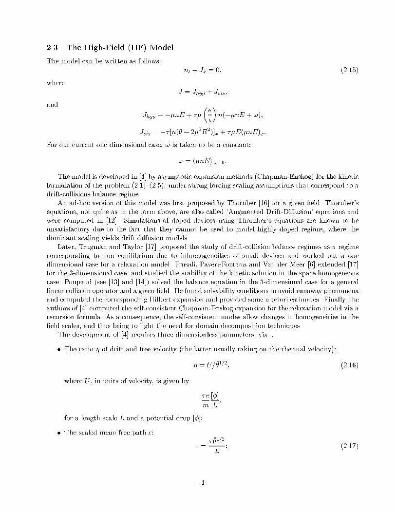
2.3 The High-Field (HF) Model.The model can be written as follows: nt + Jx = 0; (2.15)where J = Jhyp + Jvis;and Jhyp = ��nE + ���e��n(��nE + !);Jvis = �� [n(� + 2�2E2)]x + ��E(�nE)x:For our current one dimensional case, ! is taken to be a constant:! = (�nE)jx=0:The model is developed in [4] by asymptotic expansion methods (Chapman-Enskog) for the kineticformulation of the problem (2.1){(2.5), under strong forcing scaling assumptions that correspond to adrift-collisions balance regime.An ad-hoc version of this model was �rst proposed by Thornber [16] for a given �eld. Thornber'sequations, not quite as in the form above, are also called `Augmented Drift-Di�usion' equations andwere computed in [12]. Simulations of doped devices using Thornber's equations are known to beunsatisfactory due to the fact that they cannot be used to model highly doped regions, where thedominant scaling yields drift di�usion models.Later, Trugman and Taylor [17] proposed the study of drift-collision balance regimes as a regimecorresponding to non{equilibrium due to inhomogeneities of small devices and worked out a onedimensional case for a relaxation model. Frosali, Paveri-Fontana and Van der Meer [6] extended [17]for the 3-dimensional case, and studied the stability of the kinetic solution in the space homogeneouscase. Poupaud (see [13] and [14]) solved the balance equation in the 3-dimensional case for a generallinear collision operator and a given �eld. He found solvability conditions to avoid runaway phenomenaand computed the corresponding Hilbert expansion and provided some a priori estimates. Finally, theauthors of [4] computed the self-consistent Chapman-Enskog expansion for the relaxation model via arecursion formula. As a consequence, the self-consistent modes allow changes in homogeneities in the�eld scales, and thus bring to light the need for domain decomposition techniques.The development of [4] requires three dimensionless parameters, viz. ,� The ratio � of drift and free velocity (the latter usually taking on the thermal velocity):� = U=��1=2; (2.16)where U , in units of velocity, is given by �em [�]L ;for a length scale L and a potential drop [�];� The scaled mean free path ": " = � ��1=2L ; (2.17)4

� The scaled Debye length from the electrostatic potential equation of a self-consistent model: = ��eL2�[�] ; (2.18)where �� scales the density of the �xed background nd(x).For � of the same order of " and both very small as in the highly doped regions, the Chapman-Enskog expansion associated with system (2.1){(2.5) yields the DD equations (2.14). However, insidethe channel region, � becomes of order of one as well as . Here the corresponding expansion yieldsthe high-�eld model (2.15).3 SimulationThe device we consider for this paper is the one dimensional Silicon n+-n-n+ structure of length0:6�m. The device used is as follows: x 2 [0; 0:6]; the doping is de�ned by nd(x) = 5 � 105=�m3 in0 � x � 0:1 and in 0:5 � x � 0:6, and by nd(x) = 2 � 103=�m3 in 0:15 � x � 0:45, with a smoothintermediate transition. This is the Silicon device analogue of the GaAs device used by Baranger andWilkins [1], except for a smooth transition of width 0:05�m at the junctions.More speci�c conditions for various models are listed below.1. For the kinetic model (2.1):� The velocity space is arti�cially cut at �a � u � a; (3.1)where we monitor to ensure that f(x; u; t) is always very small at the boundary u = �a forthe �nal steady state results. We learned that it is more than enough in all our runs to usea = 3:5.� We use a uniform grid both in x and in u, with 160 � 150 points.� At x = 0, take f(0; u; t) = nd(0)M(u) (3.2)if u � 0, and no boundary condition (extrapolation of the numerical solution from insidethe domain to the boundary) if u < 0. Also take �(0; t) = 0.� At x = 0:6, take f(0:6; u; t) = nd(0:6)M(u) (3.3)if u � 0, and no boundary condition (extrapolation of the numerical solution from insidethe domain to the boundary) if u > 0. Also take �(0:6; t) = vbias.� At u = �a and u = a, take no boundary condition (extrapolation of the numerical solutionfrom inside the domain to the boundary).2. For the elementary domain decomposition, we apply the low �eld drift-di�usion (DD) model(2.14) in [0,A] and [B,0.6], and the high-�eld (HF) model (2.15) in (A,B). For a �xed pair (A,B),we perform the following:� We use a uniform grid in x with 160 points.5

� At x = 0 and x = 0:6, take the boundary conditionsn(0; t) = nd(0); �(0; t) = 0;n(0:6; t) = nd(0:6); �(0:6; t) = vbias:� At the interfaces x = A and x = B, there are no explicit interface boundary conditions.The coupling of the drift-di�usion model and the high �eld model is through the ghostpoints used in the computation:{ When a grid point is inside [0,A] or [B,0.6], the solution n is updated by the drift-di�usion model (2.14) using a �fth order conservative WENO scheme. Since this schemehas a 7-point stencil, when computing the updates near the interfaces A or B, the stencilactually goes into the region (A,B), hence the information in that high �eld region isused.{ Similarly, the high �eld model (2.15) is used to update the solution if the grid pointis inside (A,B). Again, the 7-point stencil of the numerical scheme implies that infor-mation inside the drift-di�usion region [0,A] and [B,0.6] is used when the grid point isnear the interfaces A and B.Simulations are performed for vbias from 0V to 1.5V, and results are shown only for vbias = 1:5Vto save space. Other parameters: m = 0:26�0:9109 (10�30Kg), e = 0:1602 (10�18C), kb = 0:138046�10�4 (10�18J=Kelvin), � = 11:7 � 8:85418 (10�18F=�m), T0 = 300K.4 Numerical AlgorithmWe use the ENO schemes developed in [15] and the weighted ENO (WENO) schemes developed in[11]. ENO and WENO schemes are designed for hyperbolic conservation laws or other problemscontaining either discontinuous solutions or solutions with sharp gradients. The guiding principle isan adaptive local choice of a stencil (ENO), or use of a nonlinear convex combination of contributionsfrom local stencils (WENO), so that contributions from stencils containing a possible discontinuity orother unpleasant features (e.g., a high gradient) are either completely avoided (ENO) or are assigneda nearly zero weight (WENO). In doing this, uniform high order accuracy can be achieved withoutintroducing any oscillations near discontinuities or sharp gradient regions. The high order accuracyof these algorithms allows us to use relatively coarse grids and still get very accurate results. Thealgorithms are extremely stable and robust in all the numerical simulations.5 Simulation ResultsIn all the numerical simulations, we perform a long time integration until a steady state is reached.In Fig. 5.1, Fig. 5.2 and Fig. 5.3 we show the results of the kinetic simulation for vbias = 1:5 voltwith various forms of mobility �, given by (2.8), (2.9), (2.10) and (2.12). Fig. 5.1 contains the resultsof concentration n, velocity v v(x; t) = Z 1�1 uf(x; u; t)du =n(x; t); (5.1)electric �eld E and potential �. Fig. 5.2 contains the results of the I-V curve withI = eb� a Z ba n(x; t)v(x; t)dx: (5.2)6

Notice that the collision integrals conserve particle number, hence n(x; t)v(x; t) should be a constantin steady states. We still take the average in (5.2) in the whole region [a; b]=[0, 0.6] to compute I.The quantity � for vbias = 1:5V , de�ned in (2.16), which is useful for the veri�cation of suitabilityfor the high-�eld model (see Section 2.3), is also plotted in Fig. 5.2. Fig. 5.3 contains the probabilitydensity function f(x; u; t)=n(x; t) at x = 0:12 and x = 0:42.For this channel, at vbias = 1:5V, the scaled mean free path " de�ned in (2.17) is in the range of0:01 to 0:07, depending on the mobility assumptions.From Fig. 5.1, Fig. 5.2 and Fig. 5.3 we can see that di�erent mobility assumptions yield signi�cantlydi�erent results, especially in velocity, and hence also a�ect the I-V curves. This indicates that, whenusing kinetic results as benchmarks, one must be careful in the mobility assumptions. Comparingwith the simulation results of the hydrodynamic model in [8], which is calibrated by Monte-Carlosimulations, we can see that the choices (2.8), (2.9) and (2.10) for the mobility produce results over-estimating the velocity, while the choice (2.12) is producing velocity at the correct magnitude. Theover-estimation of the velocity, when the more physical mobility assumption (2.10) is used, has alsobeen observed, to a lesser extent, in the work of Fatemi and Odeh [5], where two space dimensions areused in the phase space for the kinetic model. Presumably this over-estimation is an indication thatthe collision model used in the kinetic model is over-simpli�ed. Henceforth, we will concentrate ourattention on the �eld dependent mobility � = �(E) as given by (2.12).Next, we perform a preliminary domain decomposition in the channel region alone, to motivate theelementary domain decomposition to follow. This highlights the e�ectiveness of the high �eld modelin the channel region. Thus, in Fig. 5.4 (the whole region) and in Fig. 5.5 (zoomed-in pictures) we plotthe comparison among the mid-region simulations of DD and HF, and the global kinetic simulation,at vbias = 1:5V. We perform the mid-region simulation for HF and DD with the boundary conditionsprovided by the kinetic simulation using � = �(E) given by (2.12). We can see, especially in thezoomed-in pictures, that the high-�eld model has a better agreement with the kinetic simulations.Finally, we perform the elementary domain decomposition by applying the low �eld drift di�usionmodel in [0,A] and [B,0.6], and the high �eld model in (A,B). Given the concentration n at the timelevel k, for points within [0,A] and [B,0.6], the update to the next time level is via the low �eld driftdi�usion model. For points within (A,B), the update to the next time level is via the high �eld model.Interface coupling is implicit through the 7-point stencil of WENO schemes used for both models, asexplained before.The results of this elementary domain decomposition are shown in Fig. 5.6 (the whole region)and in Fig. 5.7 (zoomed-in pictures), for vbias = 1:5V , A = 0:21 and B = 0:435. We observe slightimprovement of this elementary domain decomposition over the low �eld drift-di�usion model. Forthis device the low �eld drift-di�usion model with � = �(E) as given in (2.12) is already a good model.We also observe that this elementary domain decomposition is numerically stable.References[1] H. U. Barenger and J. W. Wilkins, Ballistic structure in the electron distribution function ofsmall semiconducting structures: General features and speci�c trends. Phys. Rev. B, 36:1487{1502, 1987.[2] C. Cercignani, I. M. Gamba, J. W. Jerome and C-W. Shu. Applicability of the high-�eld model:An analytical study based on asymptotic parameters de�ning domain decomposition. VLSIDESIGN, 8:135{141, 1998.[3] C. Cercignani, I. M. Gamba, J. W. Jerome and C-W. Shu. Applicability of the high-�eld model:A preliminary numerical study. VLSI DESIGN, 8:275{282, 1998.7

[4] C. Cercignani, I. M. Gamba and C. D. Levermore. High �eld approximations to Boltzmann-Poisson system boundary conditions in a semiconductor. Appl. Math. Lett., 10:111{117, 1997.[5] E. Fatemi and F. Odeh. Upwind �nite di�erence solution of the Boltzmann equation applied toelectron transport in semiconductor devices. J. Comput. Phys., 108: 209{217, 1993.[6] G. Frosali, C.V.M. van der Mee and S.L. Paveri-Fontana. Conditions for run{away phenomenain the kinetic theory of particle swarms, J. Math. Physics 30:1177{1186, 1989.[7] J. W. Jerome. Analysis of Charge Transport: A Mathematical Study of Semiconductor Devices.Springer, 1996.[8] J. W. Jerome and C.-W. Shu. Energy models for one-carrier transport in semiconductor devices.IMA Volumes in Mathematics and Its Applications, v59, W. Coughran, J. Cole, P. Lloyd andJ. White, editors, Springer-Verlag, 1994, pp.185-207.[9] J. W. Jerome and C.-W. Shu. The response of the hydrodynamic model to heat conduction,mobility, and relaxation expressions. VLSI DESIGN, 3:131{143, 1995.[10] J. W. Jerome and C.-W. Shu. Transport e�ects and characteristic modes in the modeling andsimulation of submicron devices. IEEE Trans. Computer-Aided Design of Integrated Circuitsand Systems, 14:917{923, 1995.[11] G. Jiang and C.-W. Shu. E�cient implementation of weighted ENO schemes. J. Comput. Phys.,126:202{228, 1996.[12] E. C. Kan, U. Ravaioli and T. Kerkhoven. Calculation of velocity overshoot in submicron devicesusing an augmented drift-di�usion model. Solid-State Electr., 34:995{999, 1991.[13] F. Poupaud. Runaway phenomena and uid approximation under high �elds in semiconductorkinetic theory, Z.Angew. Math. Mech. 72:359-372, 1992.[14] F. Poupaud. Derivation of a hydrodynamic systems hierarchy from the Boltzmann equation,Appl. Math. Lett., 4:75-79, 1991.[15] C.-W. Shu and S. Osher, E�cient implementation of essentially non-oscillatory shock capturingschemes II, J. Comput. Phys., 83:32{78, 1989.[16] K. K. Thornber. Current equations for velocity overshoot. IEEE Electron Device Lett., 3:69{71,1983.[17] S.A. Trugman and A. J. Taylor, Analytic solution of the Boltzmann equation with applicationsto electron transport in inhomogeneous semiconductors, Phys. Rev. B 33, 5575{5584 (1986).
8

0 0.1 0.2 0.3 0.4 0.5 0.6
100000
200000
300000
400000500000600000
n (µm-3)
x (µm)
Kinetic, concentration n
0 0.1 0.2 0.3 0.4 0.5 0.6-0.1
0
0.1
0.2
0.3
0.4
0.5
0.6
0.7
x (µm)
v (µm/ps)Kinetic, velocity v
0 0.1 0.2 0.3 0.4 0.5 0.6-9
-8
-7
-6
-5
-4
-3
-2
-1
0
1
2
x (µm)
Kinetic, electric field EE (volt/µm)
0 0.1 0.2 0.3 0.4 0.5 0.6
0
0.2
0.4
0.6
0.8
1
1.2
1.4
1.6
x (µm)
Kinetic, potential φφ (volts)
Figure 5.1: Kinetic simulation results of vbias = 1:5 volt with various assumptions on �. Solid line:� = :1323; dashed line: � = 0:0367; dash-dotted line: � = �(nd) as given by (2.10); long dashed line:� = �(E) as given by (2.12). Top left: the concentration n in �m�3; top right: the velocity v in�m=ps; bottom left: the electric �eld E in volts=�m; bottom right: the potential � in volts.9

0 0.5 1 1.50
100
200
300
400
500
600
700
800
vbias (volts)
I (10-6 A/µm2)
Kinetic, I-V curve
0 0.1 0.2 0.3 0.4 0.5 0.6-7
-6
-5
-4
-3
-2
-1
0
1
2
x (µm)
η Kinetic, η
Figure 5.2: Kinetic simulation results with various assumptions on �. Solid line: � = :1323; dashedline: � = 0:0367; dash-dotted line: � = �(nd) as given by (2.10); long dashed line: � = �(E) as givenby (2.12). Left: the I-V curve in 10�6Amps=�m2 versus volts; right: the quantity � de�ned in (2.16)at vbias = 1:5 volt.
-3 -2 -1 0 1 2 3
0
0.5
1
1.5
2
2.5
3
u
f/n
Kinetic, f/n at x=0.12
-3 -2 -1 0 1 2 3
0
0.5
1
1.5
2
2.5
u
f/nKinetic, f/n at x=0.42
Figure 5.3: The probability density function f(x; u; t)=n(x; t) of the kinetic simulation with variousassumptions on �. Solid line: � = :1323; dashed line: � = 0:0367; dash-dotted line: � = �(nd) as givenby (2.10); long dashed line: � = �(E) as given by (2.12). Left: at x = 0:12�m; right: at x = 0:42�m.10

0 0.1 0.2 0.3 0.4 0.5 0.6
100000
200000
300000
400000500000600000
x (µm)
n (µm-3)Mid-region, concentration n
0 0.1 0.2 0.3 0.4 0.5 0.6
0.01
0.02
0.03
0.04
0.05
0.06
0.07
0.08
0.09
0.1
0.11
0.12
0.13
x (µm)
v (µm/ps)Mid-region, velocity v
0 0.1 0.2 0.3 0.4 0.5 0.6-9
-8
-7
-6
-5
-4
-3
-2
-1
0
1
2
x (µm)
E (volt/µm)Mid-region, electric field E
0 0.1 0.2 0.3 0.4 0.5 0.6
0
0.2
0.4
0.6
0.8
1
1.2
1.4
1.6
x (µm)
φ (volts)Mid-region, potential φ
Figure 5.4: The global kinetic simulation (solid line), the mid-region HF simulation (dashed line), andthe mid-region DD simulation (dash-dotted line). � = �(E) for all simulations. The global kineticsimulation provides the boundary conditions for the mid-region HF and DD simulations. Top left:the concentration n in �m�3; top right: the velocity v in �m=ps; bottom left: the electric �eld E involts=�m; bottom right: the potential � in volts.11

0.25 0.3 0.35 0.417000
18000
19000
20000
21000
22000
x (µm)
n (µm-3)Mid-region, concentration n
(zoomed-in)
0.25 0.3 0.35 0.4
0.1
0.11
0.12
x (µm)
v (µm/ps)Mid-region, velocity v
(zoomed-in)
0.25 0.3 0.35 0.4
-8
-7
-6
-5
-4
-3
-2
x (µm)
E (volt/µm)Mid-region, electric field E
(zoomed-in)
0.25 0.3 0.35 0.40
0.2
0.4
0.6
0.8
1
1.2
x (µm)
φ (volts)Mid-region, potential φ
Figure 5.5: Zoomed-in pictures. The global kinetic simulation (solid line), the mid-region HF simula-tion (dashed line), and the mid-region DD simulation (dash-dotted line). � = �(E) for all simulations.The global kinetic simulation provides the boundary conditions for the mid-region HF and DD simu-lations. Top left: the concentration n in �m�3; top right: the velocity v in �m=ps; bottom left: theelectric �eld E in volts=�m; bottom right: the potential � in volts.12

0 0.1 0.2 0.3 0.4 0.5 0.6
100000
200000
300000
400000500000600000
x (µm)
n (µm-3)concentration n
0 0.1 0.2 0.3 0.4 0.5 0.6
0.01
0.02
0.03
0.04
0.05
0.06
0.07
0.08
0.09
0.1
0.11
0.12
0.13
x (µm)
v (µm/ps) velocity v
0 0.1 0.2 0.3 0.4 0.5 0.6-9
-8
-7
-6
-5
-4
-3
-2
-1
0
1
2
x (µm)
E (volt/µm)Electric field E
0 0.1 0.2 0.3 0.4 0.5 0.6
0
0.2
0.4
0.6
0.8
1
1.2
1.4
1.6
x (µm)
φ (volts) Potential φ
Figure 5.6: The global kinetic simulation (solid line), the global DD simulation (dashed line), and theelementary domain decomposition with the HF in (0.21,0.435) and DD otherwise (dash-dotted line).� = �(E) for all simulations. Top left: the concentration n in �m�3; top right: the velocity v in�m=ps; bottom left: the electric �eld E in volts=�m; bottom right: the potential � in volts.13

0.25 0.3 0.35 0.4
18000
19000
20000
21000
22000
23000
24000
x (µm)
n (µm-3)concentration n
(zoomed-in)
0.25 0.3 0.35 0.4
0.1
0.11
0.12
x (µm)
v (µm/ps) velocity v(zoomed-in)
0.25 0.3 0.35 0.4
-8
-7
-6
-5
-4
-3
-2
x (µm)
E (volt/µm)Electric field E
(zoomed-in)
0.25 0.3 0.35 0.4
0
0.2
0.4
0.6
0.8
1
1.2
x (µm)
φ (volts) Potential φ(zoomed-in)
Figure 5.7: Zoomed-in pictures. The global kinetic simulation (solid line), the global DD simulation(dashed line), and the elementary domain decomposition with the HF in (0.21,0.435) and DD otherwise(dash-dotted line). � = �(E) for all simulations. Top left: the concentration n in �m�3; top right:the velocity v in �m=ps; bottom left: the electric �eld E in volts=�m; bottom right: the potential �in volts.14