i

MÁSTER OFICIAL EN GEOLOGÍA APLICADA

A LOS RECURSOS MINERALES Y ENERGÉTICOS

(GEOREC)

TRABAJO FIN DE MÁSTER

3D GEOMODELING OF RESERVOIR OUTCROP ANALOGS

Geomodelización 3D de análogos aflorantes de reservorios

AUTOR: LUIS MIGUEL YESTE PÉREZ

ESPECIALIDAD: RECURSOS ENERGÉTICOS

TUTORES: CÉSAR VISERAS ALARCÓN

(Catedrático de Estratigrafía en la Universidad de Granada)

NEIL MCDOUGALL

(Senior Clastic Sedimentologist Advisor en Repsol)

SEPTIEMBRE DE 2015

ii

TABLE OF CONTENTS

Abstract - Resumen ............................................................................................................................ viii

1. INTRODUCTION ............................................................................................................................. 1

2. METHODOLOGY ............................................................................................................................ 2

3. GEOLOGICAL SETTING .............................................................................................................. 2

4. DATA ACQUISITION ..................................................................................................................... 4

4.1. Zone A: Meandering System ........................................................................................................ 5

4.1.1. Outcrop description ............................................................................................................ 5

4.1.2. Well data: cores and well logs ............................................................................................ 6

4.1.3. GPR data ............................................................................................................................. 8

4.1.4. Petrophysical data: porosity and permeability ................................................................... 9

4.2. Zone B: Braided System ............................................................................................................. 10

4.2.1. Outcrop description .......................................................................................................... 10

4.2.2. Well data: cores and well logs .......................................................................................... 11

4.2.3. GPR data ........................................................................................................................... 13

4.2.4. Petrophysical data: porosity and permeability ................................................................. 14

5. GEOLOGICAL MODELING ........................................................................................................ 15

5.1. Modeling strategy ....................................................................................................................... 15

5.2. Surface modeling ........................................................................................................................ 15

5.3. Gridding ..................................................................................................................................... 16

5.4. Zones and Layering .................................................................................................................... 17

5.5. Scale up ...................................................................................................................................... 18

5.6. Data analysis .............................................................................................................................. 18

5.7. Property modeling: Facies and Petrophysical modeling ............................................................ 19

5.8. Deterministic versus stochastic algorithms ................................................................................ 19

6. RESULTS ......................................................................................................................................... 20

6.1. Zone A: Meandering System ...................................................................................................... 20

6.1.1. Surface modeling ............................................................................................................... 20

6.1.2. Model Characteristics ....................................................................................................... 20

6.1.3. Scale up ............................................................................................................................. 21

6.1.4. Data analysis ..................................................................................................................... 23

6.1.5. Facies modeling ................................................................................................................ 25

6.1.6. Petrophysical modeling ..................................................................................................... 27

6.1.7. Operations strategy ........................................................................................................... 27

6.2. Zone B: Braided System ............................................................................................................. 28

6.2.1. Surface modeling ............................................................................................................... 28

6.2.2. Model Characteristics ....................................................................................................... 29

6.2.3. Scale up ............................................................................................................................. 30

6.2.4. Data analysis ..................................................................................................................... 32

6.2.5. Facies modeling ................................................................................................................ 33

6.2.6. Petrophysical modeling ..................................................................................................... 35

6.2.7. Operations strategy ........................................................................................................... 35

7. CONCLUSIONS .............................................................................................................................. 36

8. REFERENCES ................................................................................................................................ 38

iii

APPENDIX I. LITHOFACIES TABLE .............................................................................................. I

APPENDIX II. COMPOSITE WELL LOGS ................................................................................... III

Appendix II.1. Legend for composite well logs. ............................................................................... III

Appendix II.2. Composite well log MB1. .......................................................................................... IV

Appendix II.3. Composite well log MB2. ........................................................................................... V

Appendix II.4. Composite well log MB3. .......................................................................................... VI

Appendix II.5. Composite well log MB4. ......................................................................................... VII

Appendix II.6. Composite well log K2P1. ....................................................................................... VIII

Appendix II.7. Composite well log K2P2. ......................................................................................... IX

Appendix II.8. Composite well log K2L1. .......................................................................................... X

Appendix II.9. Composite well log K2L2. ......................................................................................... XI

Appendix II.10. Composite well log K2L3. ...................................................................................... XII

Appendix II.11. Composite well log K2L4. ..................................................................................... XIII

APPENDIX III. RADAR FACIES TABLE ................................................................................... XIV

APPENDIX IV. GPR PROFILES .................................................................................................... XV

Appendix IV.1. GPR profile Bart-1. ................................................................................................. XV

Appendix IV.2. GPR profile Bart-2 and Bart-3. .............................................................................. XVI

Appendix IV.3. GPR profile Bart-4. ............................................................................................... XVII

Appendix IV.4. GPR profile Bart-5. .............................................................................................. XVIII

Appendix IV.5. GPR profile K2S-PR1 ............................................................................................ XIX

Appendix IV.6. GPR profile K2S-PR2. ............................................................................................ XX

Appendix IV.7. GPR profile K2N-PR1. ........................................................................................... XXI

Appendix IV.8. GPR profile K2N-PR2. .......................................................................................... XXII

iv

LIST OF FIGURES

Fig. 3.1. Geographical and geological location of the TIBEM. (Modified after Viseras et al., 2011; Henares et

al., 2014). ................................................................................................................................................................. 3

Fig. 3.2. TIBEM stratigraphic succession in the Alcaraz area (On the left). On the right the conceptual models

and current analog of a meandering and a braided system are shown (modified after Dabrio and Fernandez,

1986). ....................................................................................................................................................................... 4

Fig. 4.1. Adquisition data workflow. ....................................................................................................................... 5

Fig. 4.2. Location and outcrop interpretation of the studied meandering system. A) shows the satellite image

with the location of outcrop in green, the drilled wells with red points and GPR profiles with yellow lines. Figure

B shows a view of the outcrop and wells located behind it. C) represents the overall interpretation of the

structure of the outcrop. D) shows the interpretation of channel sub-environment. E) represents the detail of the

point bar in its central part. Figure F shows the detail of the point bar in its distal part. G) shows in detail one of

the chute channels interpreted. ................................................................................................................................. 7

Fig. 4.3. A) and B) Photomicrographs of detrital and diagenetic fabrics. Notice the pervasive cementation in A)

and the heterogeneity caused by the detrital matrix in B). C) Spatial distribution model of diagenetic processes

and detrital matrix content (Modified after Henares et al., 2015). ......................................................................... 10

Fig. 4.4. Location and outcrop interpretation of the braided system. A) shows the satellite image with the

location of outcrop in green, the drilled wells with red point and GPR profiles with yellow lines. B) shows a

panoramic of the northern outcrop and location of 4 wells in it. C) represents the northern outcrop interpretation.

D) shows an overview of the southern outcrops and location of well in them. E) represents the interpretation of

the outcrop in the north channel and compound bar (Outcrop S-1). F) represents the interpretation of the south

outcrop corresponding to compound bar (Outcrop S-2). G) shows the detailed interpretation of the south channel

(Outcrop S-3). ........................................................................................................................................................ 12

Fig. 4.5. A) Conceptual model and location of the samples for porosity and permeability. B) Photomicrographs

of detrital fabric. Notice the high intergranular primary porosity represented by blue colour. (Modified after

Henares et al., 2014). ............................................................................................................................................. 14

Fig. 5.1. Modeling workflow designed for the study examples. ............................................................................ 16

Fig. 5.2. Example of surface modelling (Modified after Schlumberger). .............................................................. 16

Fig. 5.3. Example of Gridding process. ................................................................................................................. 16

Fig. 5.4. Grid Resolution. Example of the Colosseum in Rome (Modified after Edwards et al., 2012). ............... 17

Fig. 5.5. Differences between Zones and Layering (Modified after Schlumberger). ............................................. 17

Fig. 5.6. A) Concept of Scale up. B) Example of Scale up in the wells. C) Example of Scale up in the logs

(Modified after Schlumberger). ............................................................................................................................. 18

Fig. 5.7. Example of Data analysis (Modified after Schlumberger). ..................................................................... 18

Fig. 5.8. Property modeling examples (Modified after Schlumberger). ................................................................ 19

Fig. 6.1. Surfaces modeling for the meandering system study example. A and B) show the surface modeling for

stochastic method. C and D) show the surface modeling for deterministic method. ............................................. 21

Fig. 6.2. Lithofacies Scale up. In the right column it is shown the upscaling of lithofacies. In orange appears

channel, in yellow the point bar and in green the flood plain facies. ..................................................................... 22

Fig. 6.3. Scale up of petrophysical data in wells MB3 and MB4. A) Facies logs. B and D) Porosity and

permeability logs. C and E) Result of upscaling.. .................................................................................................. 23

Fig. 6.4. Data analysis of facies, porosity and permeability for the meandering system study example. .............. 23

Fig. 6.5. Cross plot of porosity versus permeability. ............................................................................................. 24

v

Fig. 6.6. Quality control between well logs and upscaled data. ............................................................................. 24

Fig. 6.7. Variogram that describes the relationship between porosity and permeability. ...................................... 25

Fig. 6.8. Facies models. A-C) show the little geometric fit of facies models generated by stochastic methods. D)

shows how these examples above did not conform fully to the input data of wells. E) represents the facies model

generated deterministically. F) shows how the deterministic facies model is adjusted to the input data. The

legend of all figures is represented in figure F on the upper right margin. ............................................................ 26

Fig. 6.9. Quality control of the deterministic model with outcrop. For the legend of the colors see Fig. 6.8 F. .... 26

Fig. 6.10. Porosity and Permeability models. On the left the 3D porosity model is displayed (A) and its testing

with the outcrop section (B). On the right the 3D permeability model is displayed (C) and its testing with the

outcrop section (D)................................................................................................................................................. 27

Fig. 6.11. Wells design for the exploiting strategy of this study example as outcrop analog. A) shows the design

of vertical boreholes. B) shows the design of deviated boreholes. C) shows the design of horizontal boreholes. . 28

Fig. 6.12. Surfaces modeling for the braided system study example. A and B) show the surface modeling for

stochastic method. C and D) show the surface modeling for deterministic method. ............................................. 29

Fig. 6.13. Lithofacies Scale up for the braided system example. In the right column it is shown the upscaling of

lithofacies. The channel appears in orange and in yellow the compound bar. ....................................................... 31

Fig. 6.14. Scale up of petrophysical data in wells K2P1 and K2P2. A) Facies logs. B and D) Porosity and

permeability logs. C and E) Result of upscaling. ................................................................................................... 31

Fig. 6.15. Data analysis of facies, porosity and permeability. ............................................................................... 32

Fig. 6.16. Cross plot of porosity versus permeability. ........................................................................................... 32

Fig. 6.17. Quality control between well logs and upscaled data. ........................................................................... 33

Fig. 6.18. Variogram that describes the relationship between porosity and permeability...................................... 33

Fig. 6.19. Facies model. A-C) show the little geometric fit of facies models generated by stochastic methods. D)

shows how the deterministic facies model is adjusted to the input data (outcrop). E) represents the facies model

generated deterministically. On its lower left margin the legend is presented. ...................................................... 34

Fig. 6.20. Quality control of the deterministic model with outcrop. For the legend of the colors see Fig. 6.19 E. 35

Fig. 6.21. Porosity and Permeability models for the braided system study example. On the left the 3D porosity

model (A) and its testing with the outcrop section (B) are displayed. On the right the 3D permeability model (C)

and its testing with the outcrop section (D) are shown. ......................................................................................... 35

Fig. 6.22. Wells design for the exploiting strategy of this study example as outcrop analog. A) shows the design

of vertical boreholes. B) shows the design of horizontal boreholes. C) shows the design of boreholes combining

previous designs (A and B). ................................................................................................................................... 36

vi

LIST OF TABLES

Table 4.1. Porosity and Permeability data obtained for meandering example. ...................................................... 9

Table 4.2. Porosity and permeability data obtained for the braided example. The code column represents the

abbreviation shown in Fig. 4.5. ............................................................................................................................. 14

Table 6.1. Grid, zones and layers characteristics in the models of the meandering system. ................................ 22

Table 6.2. Geometrical inputs controlling the body shape. .................................................................................. 25

Table 6.3. Grid, zones and layers characteristics of the models of the braided system. ....................................... 30

Table 6.4. Geometrical inputs controlling the body shape. .................................................................................. 33

vii

Agradecimientos

En primer lugar agradecer a mis directores de éste trabajo de fin de máster: Dr. César Viseras por su

confianza depositada en mí así como su compromiso para llevar a cabo este trabajo y Dr. Neil

McDougall por su ofrecimiento a dirigir este trabajo así como por su acogimiento y por el tiempo

empleado durante mi estancia en Repsol. Agradecer a Dña. Saturnina Henares sus ideas, colaboración

y su permanente disponibilidad. También agradecer a Ricardo Palomino, geólogo de desarrollo en

Repsol, por sus aportaciones en conocimientos de modelización. También quisiera agradecer la

colaboración de Dr. Juan Fernández, cuya experiencia sobre el terreno ha sido imprescindible.

Mencionar también a D. Javier Jaímez, técnico del CIC, sin la ayuda y trabajo del cual no habría sido

posible la obtención de estos resultados así como a los Dres. Teresa Teixidó y José Antonio Peña por

la labor empeñada en su trabajo así como el aporte de conocimientos transmitidos.

Agradecer a Repsol y a su Grupo de Disciplinas Geológicas, y particularmente a Tomás Zapata y

Jorge Peña, por brindarme la oportunidad de llevar a cabo este trabajo gracias al disfrute de una de las

becas ofrecidas para este máster, así como por el caluroso acogimiento para la estancia en prácticas

realizada en sus instalaciones.

Agradecer a Dr. Alberto Pérez, coordinador del máster GEOREC, por su trabajo realizado en todos los

trámites administrativos del máster y al equipo docente del máster por su enriquecedor aporte

académico en este curso 2014-2015.

Agradezco a Schlumberger la concesión de la licencia 2-1394908 de Petrel al proyecto al cual está

ligado este trabajo y a D. Jacobo Marquis por sus funciones administrativas para que esta licencia haya

estado disponible a tiempo.

Por último, agradecer al proyecto CGL 2013 43013 R y al Grupo RNM 369 del Plan Andaluz de

investigación la financiación necesaria para la realización de este trabajo.

viii

Abstract

From geometric, sedimentological and petrological characteristics derived in outcrop and cores and

well logging data of boreholes in combination with GPR lines, two 3D models of two examples

belonging to the red beds of TIBEM (Triassic of the Iberian Meseta, Spain) is constructed. One of the

selected examples corresponds to a meander belt in which the main highly sinuous channel, the point

bars associated with the main channel, multiple scroll bars attached to one of the point bars and two

chute channels are distinguished for modeling. The other example selected corresponds to a braided

system in which two channels and two compound bars are distinguished for modeling. The models

have been obtained by applying the Petrel software. Modeling has been carried out by both stochastic

and deterministic methods, being the last one which shows quite realistically heterogeneities within

the reservoir facies. On the other hand the stochastic methods have differentiate fairly well zones of

greater and lesser value porosity and permeability, controlled by the distribution of lithofacies between

different sub-environments. These examples are revealed as some interesting similar outcrops analogs

to many fluvial reservoirs, demonstrating the usefulness of this research in order to exploit

hydrocarbon reservoirs.

Key-words: outcrop analog, meanderbelt, braided, facies, modeling, 3D geomodel, Ground

Penetrating Radar (GPR), Triassic.

Resumen

A partir de las características geométricas, sedimentológicas y petrológicas deducidas en afloramiento

y con datos de testigos de sondeos y sus diagrafías, en combinación con líneas de GPR, se proponen

dos modelos tridimensionales de dos ejemplos distintos pertenecientes a las capas rojas del TIBEM

(Cobertera Triásica de la Meseta Ibérica). Uno de los ejemplos seleccionados corresponde a un

sistema meandriforme en el que se distinguen para su modelización el canal principal sinuoso, las

barras de meandro asociadas al canal principal, varias barras de scroll asociadas a una de las barras de

meandro y dos canales de chute. El otro ejemplo seleccionado corresponde con un sistema trenzado en

el que se distinguen para su modelización dos canales y dos barras compuestas principales. Los

modelos han sido obtenidos mediante la aplicación del software Petrel. Se han realizado las

modelizaciones tanto por métodos estocásticos como por métodos determinísticos, siendo estos

últimos los que muestran de manera bastante realista las heterogeneidades de las facies dentro del

reservorio, mientras que los métodos estocásticos han diferenciado bastante bien las zonas de mayor y

menor valor de porosidad y permeabilidad, controladas por la distribución de litofacies entre los

distintos subambientes. Estos ejemplos se revelan como unos interesantes análogos aflorantes para

muchos reservorios fluviales, poniendo de manifiesto la utilidad de esta investigación de cara a la

explotación de yacimientos de hidrocarburos.

Palabras clave: Análogo aflorante, meandriforme, trenzado, facies, modelización, geomodelo 3D,

georrádar, Triásico.

1

1. INTRODUCTION

The outcrops of sedimentary rocks have traditionally been a good source of data for carrying out

interpretations applied to subsurface exploration and exploitation of hydrocarbon deposits. The study

of outcrops has been increasing to understand geometry and architecture of the reservoirs and to

evaluate the effects that variations in these parameters could have on production operations

(Hutchinson et al., 1961. Dodge et al., 1971). The depositional architecture is often identifiable in

outcrops, since they offer the opportunity to improve the understanding of geometry and facies

distribution of the reservoirs in the underground (Pringle et al., 2006).

The use of geological analogs for improving reservoir characterization has been addressed by many

authors (Alexander, 1992; Bryant et al., 2000; Enge et al., 2007) and it is a recognized way to improve

the prediction of 3D geometries in the laterally restricted subsoil sets data. In the last 20 years, studies

involving the use of reservoir modeling software to play outcrops, as a tool to visualize and test the

behavior of analogous reservoir is increasingly common (Bryan et al., 2000).

The outcrop analogs of comparable systems are used to provide the input parameters for the reservoir

models when subsurface data are limited. During the operational phase of field, the analogs are used to

improve understanding of the geological controls about the production and are used as a quality

control in the development of dynamic models.

The fluvial systems are one of the most studied and modeled sedimentary environments since they

hold about 20% of hydrocarbon reserves in the world and therefore are a significant kind to the oil and

gas industry storage (Keogh, 2007). However, the greatest difficulty of fluvial deposits is the degree

and extent of complexity in the architecture and heterogeneity of facies.

In order to make realistic models of a reservoir and its behavior, a quantitative description of the

reservoir is required. This description should be consistent with the subsurface data and should also

correspond to the interpretation of depositional environment and the geological history of the area.

The empirical relationships derived from analog studies are widely used in building models to improve

understanding of the system, to complement the data sets and to enable the application of stochastic or

other kind of models. Because it is impossible to create a geological model of the reservoir that is

quite geologically correct, the main objective is to capture the elements that control the production

characteristics.

Static models of reservoirs describe the external geometry, facies distribution and petrophysical

properties of rocks in the subsurface. Since in clastic reservoir the petrophysical properties (e.g.

permeability, porosity) usually correlate with sedimentary facies, facies models also allow to predict

the connectivity within the reservoir rock. Static models are one of the main input parameters for the

simulation of fluid flow (dynamic models). The reliability and quality of distribution models of facies

will influence in the final prediction (Cabello et al., 2006).

With the development of this Master Thesis it is set out to make the modeling of two analogs outcrop

examples of two different fluvial systems, a meandering system and a braided system, which are found

in TIBEM red beds (Triassic Cover of the Iberian Meseta). The study is based on the integration of

data from outcrops, subsurface data and petrophysical data in order to develop a static model of each

type of outcrop. Moreover, a workflow for modeling and a comparison between different modeling

methods is developed.

2

This work forms part of the results of research carried out by the Sedimentary Reservoirs Workgroup

(SEDREGROUP), as part of the project "Continental rock formations as potential conventional and

unconventional reservoirs: outcrop and subsurface characterization (Ref: CGL 2013 43013 R)."

2. METHODOLOGY

The first step consists in selecting outcrop study examples, getting that they have good quality as

analogous outcrops (Enge et al., 2007). Once selected the examples of study we continue with the

sedimentological characterization of these outcrops.

In order to improve both the relationship between outcrop and subsurface data to provide a direct

comparison between the typical data we have in oil reservoirs (such as cores and well logs) and the

outcrop, there have been developed several drilling campaigns following Outcrop/Behind Outcrop

(O/BO) methodology that consist of carrying out the drilling, previously scheduled, at a rear location

at the outcrop. In these campaigns, the drillings were made with core recovery and well logging using

various sondes as GR (Gamma Ray), SGR (Spectral Gamma Ray), OBI (Optical Borehole Image) and

ABI (Acoustic Borehole Image). The equipment used is part of the Drilling and Well Logging Rocks

Unit from Centre of Scientific Instrumentation, University of Granada.

Following previous indications of other authors such as Pringle et al., (2006), the Ground Penetrating

Radar (GPR) was chosen as geophysical method because it is a high-resolution technique that uses

frequencies that are 1 order of magnitude higher than shallow seismic. This results in an increase in

resolution taking into account the depth of study. GPR is used increasingly for the study of outcrop

analogs (Corbenau et al., 2001; Zeng et al., 2004; Van Den Bril et al., 2007; Kostic et al., 2007;

Hugenholtz et al., 2007; Rice et al., 2009; Pascucci et al., 2009; Nielsen et al., 2009; Bourquin et al.,

2009; Szerbiak et al., 2010; Calvache et al., 2010; Slowik, 2011; Jorry et al., 2011; Beidenger et al.,

2011; Lunt et al., 2013; Abatan et al., 2013; Ressink et al., 2014; Franke et al., 2015). Several GPR

campaigns were designed, with planned locations, to capture subsurface information with this method

in the outcrops which are under study. The campaigns were conducted in collaboration with Dr.

Teresa Teixidó and Dr. José Antonio Peña (Instituto Andaluz de Geofísica, University of Granada).

Having collected the field data, all of them were interpreted, starting with a description of lithofacies

of cores, well logs interpretation and interpretation of GPR profiles. Parallel to this work petrological

and petrophysical study has been carried out by other members of the research group for getting the

porosity and permeability data.

The next step was the processing and integration of all data for modeling. Based on these data, it has

been developed an optimal workflow modeling for these examples. Finally, static modeling has been

carried out, both facies and distribution of petrophysical properties of the studied outcrops.

3. GEOLOGICAL SETTING

Triassic red beds of the Tabular Cover of the Iberian Meseta (TIBEM) (Viseras et al., 2011) appear

between the Iberian Massif to the North (Central Iberian Zone) and the Betic Cordillera to the South

(External Zones; see Fig. 3.1). This corresponds to the Chiclana de Segura Formation according to

López Garrido, 1971. The basin is part of the continental area which was developed during the

Tethyan continental rifting process (Late Permian-Upper Triassic; Sánchez-Moya et al., 2004; Critelli

et al., 2008). The Anisian-Norian succession is about 250 m thick and organised in four subhorizontal

3

depositional sequences (I to IV according to Fernández and Dabrio, 1985). The succession consists of

siliciclastic alluvial-lacustrine and fluvial facies that directly overlie the Paleozoic basement. Each

sequence is developed under the same base level conditions controlled by the fluctuations of the

Tethys level (Haq et al., 1987; Fernández et al., 1993, 2005). Other authors as Arche et al. (2002)

subdivide the stratigraphic succession into three units that were produced by minor regression-

transgression cycles during a general sea level rise.

As paleocurrent data indicate, the main drainage directions were W-E and SW-NE with the section in

Alcaraz (Albacete, SE Spain) proving to be the most distal part of the TIBEM outcrop (Fernández and

Dabrio, 1985; Henares et al., 2011). The succession is about 160 m thick and it includes, from the base

to the top, sequences II, III (Buntsandstein facies) and IV (Keuper facies) (see Fig. 3.2). Sandstone

bodies and micritic carbonate levels from silt-rich sequence II were deposited in a floodplain including

channels (meandering and straight) and overbank deposits (crevasse splay lobes and sheet flood

deposits) (Viseras and Fernández, 1994) during a general base level rise (see Fig. 3.2). Channel bodies

are 3-7 m thick and several decametres long, while overbank deposits vary from 1 to 3 m in thickness

and 30 to several hundred metres in lateral extent (Fernández and Dabrio, 1985). A widespread

development of calcrete paleosols coincides with a falling base level (Fernández et al., 1993) which

accompanies the deposition of sequence III. A bank of sandstone 20 m thick and 100 km long

corresponds to a braidplain depositional system, and marks the beginning of sequence IV (Fernández

et al., 2005; Viseras and Fernández, 2010, see Fig. 3.2). A gradually more rapid elevation of the base

level caused the deposition of silt rich facies corresponding to a coastal plain facies and intertidal

sabkha evaporites. Shallow marine dolostones of the Imón (or Zamoranos) Formation (Upper Triassic-

Lower Jurassic) overlap and cover the sequence IV (Goy and Yébenes, 1977; Pérez-López et al.,

1992).

At regional scale, a slight tilting to the North (dip < 10º) of Triassic deposits is recognized caused by

syndepositional or gravitational compaction (sensu Gay, 1989) when sediments adapted to the

irregular topography of the Paleozoic basement.

Fig. 3.1. Geographical and geological location of the TIBEM. (Modified after Viseras et al., 2011; Henares et

al., 2014).

4

Fig. 3.2. TIBEM stratigraphic succession in the Alcaraz area (On the left). On the right the conceptual models

and current analog of a meandering and a braided system are shown (modified after Dabrio and Fernandez,

1986).

4. DATA ACQUISITION

On the base of the prior knowledge that exists about the area and examples of study, partly published

(Fernández, 1977, 1984; Fernández and Dabrio, 1985; Dabrio and Fernández, 1986; Fernandez and

Gil, 1989; Fernández et al., 1993, 1994, 2005; Viseras and Fernández, 1994; Fernández and Viseras,

2004; Fernández and Perez Lopez, 2004; Henares 2011; Henares et al., 2013; Yeste et al., 2014) and

using the experience in the area of researchers of the research group in which this work is

encompassed, it was carried out the first process of this workflow which consist of the selection of the

outcrops and the planning and determination of the various field campaigns. Later, it was continued

with design and development of drilling, well logging and GPR surveys (see Fig. 4.1).

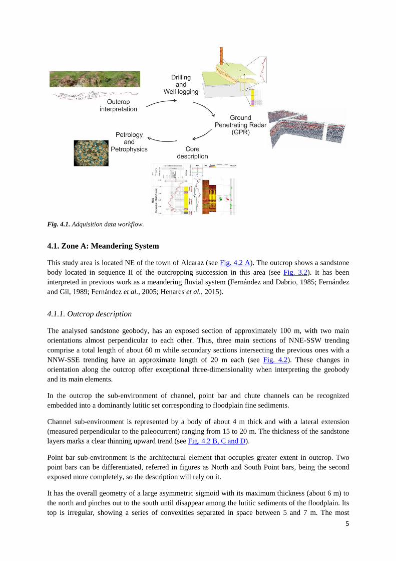
After collecting the data we continued with the integrated study of the description of the well and well

logs for the definition of lithology, facies from the different sub-environments and correlations;

interpretation of GPR profiles and their correlation to the wells; and finally, the petrological and

petrophysical study to determine the porosity and permeability of the different sub-environments

under study (see Fig. 4.1).

Miall, 1996

Miall, 1996

5

Fig. 4.1. Adquisition data workflow.

4.1. Zone A: Meandering System

This study area is located NE of the town of Alcaraz (see Fig. 4.2 A). The outcrop shows a sandstone

body located in sequence II of the outcropping succession in this area (see Fig. 3.2). It has been

interpreted in previous work as a meandering fluvial system (Fernández and Dabrio, 1985; Fernández

and Gil, 1989; Fernández et al., 2005; Henares et al., 2015).

4.1.1. Outcrop description

The analysed sandstone geobody, has an exposed section of approximately 100 m, with two main

orientations almost perpendicular to each other. Thus, three main sections of NNE-SSW trending

comprise a total length of about 60 m while secondary sections intersecting the previous ones with a

NNW-SSE trending have an approximate length of 20 m each (see Fig. 4.2). These changes in

orientation along the outcrop offer exceptional three-dimensionality when interpreting the geobody

and its main elements.

In the outcrop the sub-environment of channel, point bar and chute channels can be recognized

embedded into a dominantly lutitic set corresponding to floodplain fine sediments.

Channel sub-environment is represented by a body of about 4 m thick and with a lateral extension

(measured perpendicular to the paleocurrent) ranging from 15 to 20 m. The thickness of the sandstone

layers marks a clear thinning upward trend (see Fig. 4.2 B, C and D).

Point bar sub-environment is the architectural element that occupies greater extent in outcrop. Two

point bars can be differentiated, referred in figures as North and South Point bars, being the second

exposed more completely, so the description will rely on it.

It has the overall geometry of a large asymmetric sigmoid with its maximum thickness (about 6 m) to

the north and pinches out to the south until disappear among the lutitic sediments of the floodplain. Its

top is irregular, showing a series of convexities separated in space between 5 and 7 m. The most

6

remarkable feature of its internal structure is a mega cross-bedding inclined 13-15º to the NW.

Towards the middle part of the sigmoid a planar cross-bedding structure is recognized. In the highest

part of the sigmoid, small-scale structures are abundant (ripples and climbing ripples) (see Fig. 4.2 B,

C, E and F).

In two positions, the top of point bar appears crossed by erosive scars on which channel-geometry

symmetrical bodies are installed. These bodies have a lateral extent of up to 3 m and a maximum

thickness ranging 70-80 cm. An internal lamination is recognized that adjust with the erosional based

body and which lies unconformably with respect to the lamination of the upper point bar. These

elements are interpreted as chute channels (see Fig. 4.2. B, C and G).

4.1.2. Well data: cores and well logs

For this example a campaign of 4 wells with fully-core recovery and well logging was carried out

(MB1-4) (see Fig. 4.2 for location) so each sub-environments interpreted earlier in outcrop was

drilled. Then we proceeded to the description and interpretation of the cores and well logs. For a

detailed description of lithofacies a table of lithofacies was developed (see Appendix I).

The MB1 (see Appendix II.2) and MB2 (see Appendix II.3) wells drilled the point bar (scroll bar) and

chute channel sub-environments of the sandstone body. The MB3 (see Appendix II.4) and MB4 (see

Appendix II.5) wells drilled the point bar and channel sub-environments, in its central part by the MB4

and in its most marginal part by MB3 (see Fig. 4.2 B).

In the central area of the channel (well MB4) a fining and thinning upward (FTU) sequence is shown.

On a rich weakely imbricated mud intraclasts centimeter bed (lithofacies Gmh), a set of trough cross

beds of 60 cm thick (St) is implanted. It is overlapped by an alternation of sandstone with ripples (Sr)

and siltstone with horizontal lamination or ripples (Fl). Several erosional scars can be observed

especially towards the top of the succession. Finally, the succession is topped by a 2 m thick bed of

horizontally laminated claystone (Fl) with abundant rizoliths and some decimeter intercalation of

siltstone with ripples.

In a marginal area of the channel (well MB3) at least two erosional scars covered by a sandstone bed

with abundant mud intraclasts (Gmh) stand out in succession which are overlapped by sandy facies

with planar cross lamination (Sp) and wave lamination (Srw).

The GR curve is very different at the center and the edge of the channel. In the central part of the

channel, it shows a clear bell type trend, although its base form is not sharp, showing an unusual API

high value. At the edge of the channel, the bottom of the curve shows a saw teeth trend and only a bell

trend can be seen from the internal erosional scar upwards a bell trend can be seen although it is quite

irregular.

The tadpoles in the central part of the channel indicate almost horizontal surfaces (with dip less than

10° North), which can be returned to the horizontal when taking into account the previously mentioned

regional tilting. In this central part (well MB4) the tadpoles corresponding to cross beds indicate

directions of movement towards S and W. However, in the marginal part of the channel (well MB3)

the main channel surfaces do not appear as horizontal but inclined in the same direction as the

underlying lateral accretion units and with a dip value gradually decreasing upwards. In this marginal

sector, cross beds indicate paleocurrent direction towards the N and NNW.

7

Fig. 4.2. Location and outcrop interpretation of the studied meandering system. A) shows the satellite image with the location of outcrop in green, the drilled wells with red points and GPR

profiles with yellow lines. B) shows a view of the outcrop and wells located behind it. C) represents the overall interpretation of the structure of the outcrop. D) shows the interpretation of

channel sub-environment. E) represents the detail of the point bar in its central part. F) shows the detail of the point bar in its distal part. G) shows in detail one of the chute channels

interpreted.

8

Regarding the point bar sub-environment, it can observed the repetition of a series of cycles with

slightly erosive base, on which a decimeter-centimeter thick bed composed of mud intraclasts (Gmh)

and a set of low angle planar cross bedded sandstone (Slp) of thickness ranging between 10 and 60 cm

are developed. The last one is eventually covered by a centimetric layer of horizontally laminated

claystone-siltstone (Fl). It is noticeable the assessment of a contrary inclination between this claystone

layer and the cross bedded sandstone sets.

GR signal may show a bell pattern, as much in the part of scroll bar (wells MB1 and MB2) as in the

central part of the called point bar S (well MB3). In this last sector, however, at the base of the bell a

high API value appears punctually. In MB4, where a not outcropping third point bar is cut and located

to the south of the two exposed, the pattern at the bottom is very irregular, although the upper part

shows the typical bell pattern described before.

The tadpoles identified as corresponding to the major surfaces highlight a turn along the outcrop of the

point bar element S. Thus, in the well MB1 (southern sectors of the element) tadpoles are inclined

towards SE and ESE whereas in MB2, located more to the N, they are inclined towards ESE and

finally in MB3 (more on N) they do it to the NE. Meanwhile tadpoles which correspond to minor cross

beds indicate oblique upward direction movements and upward movement relative to inclination of the

major surfaces.

The analysis of the upwards evolution of tadpoles corresponding to the major surfaces on each of the

three wells which cut the point bar S element indicate a trend of counter-clockwise rotation

(sometimes in a timid way), whereas the rotation is clockwise in the surfaces of the point bar element

and it is cut in the well MB4, situated to the E of the previous ones.

In chute channel sub-environments is remarkable that its base is always erosive, and it may also

appear some other internal erosional scars. In one of the two identified examples a decimeter thick

layer of mud clasts is developed overlapping the scar, although the dominant lithofacies in both cases

is sandstone with ripples (Sr).

This element is presented with an insufficient thickness to that a tendency of GR with a genetic

significance may be identified.

4.1.3. GPR data

For this section of the study, a GPR survey was carried out where five profiles were performed (see

Fig. 4.2 for location) using an antenna of 200 Mhz.

With the goal of obtaining a detailed description of the observed characteristics in each profile to

recognize the different sub-environments, a table of the identified radarfacies has been designed (see

Appendix III). It will be referred in the description.

In the sub-environment of the channel dominate the mounded type radarfacies although some

subparallel layers are recognized with length up to 5 m. It is very clear the difference between the

various stages of channel building because in the lower part the reflectors show medium amplitudes

with mounded pattern, in the middle part the amplitudes increase and at the top, the amplitudes

decrease again as in the lower part. According to these geophysical data, it is a typical asymmetrical

section of the channel with an internal gently sloping accretionary bank and an external steep erosion

bank (see Appendix IV.3).

9

In the point bar sub-environment the characteristic radarfacies are composed by short slightly dipping

(5-9º) reflectors lying against major and continuous surfaces that dip in the opposite direction. The

main reflectors show locally a convex up geometry. Moreover the ridges interpreted as scroll bars can

be observed (see Appendix IV.1 to 4).

The radarfacies from the chute channel are of very low amplitude (almost free reflection). Locally,

weakly marked with little continuity mounded or chaotic elements can be recognized (see Appendix

IV.1).

The description and interpretation of these GPR profiles has allowed the identification of different

surfaces which define the main identified sub-environments. It is a very important point of view to the

subsequent modeling.

4.1.4. Petrophysical data: porosity and permeability

Petrophysical data of porosity and permeability have been provided by the research group in which

this work is included (SEDREGROUP). Some of them have been published by Henares et al. (2015).

To determine the porosity, samples were taken from the cores at different depths, according to the

representation of the different interpreted sub-environments. Then, they were analyzed by using

mercury injection-capillary pressure which allowed to obtain quantitative data on the open porosity of

the rock (see Table 4.1).

The permeability values (see Table 4.1) were obtained from the data of porosimetries and the mercury

percentage (%) corresponding of the pore radius (cumulative) 25 μm. For this purpose, Pittman’s

equation was used (Pittman, 1992):

𝐿𝑜𝑔 𝐾 = −1.221 + 1.415 𝐿𝑜𝑔∅ + 1.512 𝐿𝑜𝑔 𝑟25

Where K is the permeability, ∅ is the porosity and r25 is the percentage of total mercury corresponding

to the pore radius (cumulative) of 25 μm.

Table 4.1. Porosity and Permeability data obtained for meandering example.

10

According to Henares et al. (2015) is it concluded that the highest value of porosity and permeability

are recorded in the margin of the channel and in the scroll bar, whereas the lowest are associated to the

center of the channel and the point bar base and chute channels. This can be explained by the

occurrence of several diagenetic processes affecting the petrophysical properties (porosity and

permeability) of the sedimentary geobody. In the margin of the channel and the scroll bar there is a

higher proportion of matrix, which results in greater compaction but prevents pervasive cementation.

Therefore, in these areas primary porosity is preferentially preserved which results in higher

permeability values. The channel center, the point bar base and chute channels have a secondary

porosity produced by the dissolution of cements and feldspar grains that can improve or not pore

network connectivity. As a result, lower permeability values occur in these sub-environments (see Fig.

4.3).

Fig. 4.3. A and B) Photomicrographs of detrital and diagenetic fabrics. Notice the pervasive cementation in A)

and the heterogeneity caused by the detrital matrix in B). C) Spatial distribution model of diagenetic processes

and detrital matrix content (Modified after Henares et al., 2015).

4.2. Zone B: Braided System

This area of study is located to the E and NE of the town of Alcaraz (see Fig. 4.4 A). The outcrop is

part of a sandstone geobody about 20 m thick and kilometric lateral continuity located in the sequence

IV of the succession of this area and corresponds to K2 unit of the Keuper facies (see Fig. 3.2). This

outcrop has been interpreted as corresponding to a braided type fluvial system (Fernández et al., 1993;

Arche et al., 2002; Fernández et al., 2005; Viseras et al., 2010; Henares et al., 2014).

4.2.1. Outcrop description

The internal structure of this tabular sandstone gebody consists in parallel lamination of upper flow

regime, cross-bedding of different scales due to migration of different kind of bedforms and parallel

lamination of low flow regime. Complete vertical succession results from stacking of several smaller

thinning-upward sequences (Dabrio and Fernandez, 1986; Fernandez et al., 2005; Viseras and

Fernandez, 2010).

11

Looking at a slightly oblique direction to the main paleocurrent in the landscape two distinct parts are

recognized within the sandstone unit: a massive part, where internal erosional scars are only identify

drawing irregular concave-up surfaces (see Fig 4.4 E), and another part of the unit, where a mega-

cross-bedding inclined towards the west is shown (see Fig. 4.4 E).

These two parts correspond to the main environments which are differentiated in a perennial deep

braided system, channel and compound bar (or sand flat), respectively (Ashmore, 1982; Cant and

Walker, 1978).

In a panoramic NS (see Fig. 4.4 D) two channels can be identified, a north channel and a south

channel, and a compound bar complex between them.

The North channel has a thickness of about 20 m and a lateral extent of 250 m. In it a finning and

thinning upward sequence of channel filling is observed. Above a flat bottom of horizontal lamination

o upper flow regime dunes and megaripples are stacked hierarchically into several smaller thinning

upward sequences. The boundaries between them are marked by clay sheets indicating the temporary

abandonment of the channel associated with changes in its position (Dabrio and Fernández, 1986) (see

Fig. 4.4 E). South channel, which has similar characteristics to the previous one, has also a thickness

of about 20 m and a lateral extension of about 160 m.

Regarding the compound bar (or sand flat) sub-environment, if one of these bodies is individualized,

the dimension can be estimated in about 500 m of width and no less than 1000 m in length parallel to

the main paleocurrent. Towards the base it is observed a thick set of planar cross-bedding,

corresponding to the construction of a transverse bar on which the sand flat is installed (Fernández et

al., 2005). Above, it is recognized a succession of sets of planar and trough cross-bedding, with

upward decreasing thickness. These sets are associated with the development of a sand flat system in

which the accommodation space is gradually reduced by reducing the water column on the sand body

(see Fig. 4.4 F).

In the outcrop situated to the north of Alcaraz (see Fig. 4.4 B and C) we can see the tail of a compound

bar and its transition to a channel located downstream. Sedimentation in this channeled area is

characterized by stacking of small sequences with a decreasing thickness towards the top. Each of

these sequences is constructed by hierarchical stacking of bedforms (dunes and megaripples). The

termination of the bar in the channel results in a series of characteristic units, with sigmoidal cross

stratification geometry, which has been mentioned by some authors as delta foreset (Cant and Walker,

1978).

4.2.2. Well data: cores and well logs

In this example a total of six wells were drilled in order to obtain subsurface information (core and

well log) of each of the sub-environments identified on outcrop (K2P1-2 and K2L1-4) (see Fig. 4.4

A). Then we proceeded to the description of the core and interpretation of well logs. For a detailed

description of lithofacies a table was developed (see Appendix I).

The well K2P1 (see Appendix II.6) is located behind the outcrop of channel sub-environment (south

channel) (see Fig. 4.4 D), well K2P2 (see Appendix II.7) is drilling the compound bar sub-

environment (see Fig. 4.4 D) and the four boreholes named K2L1-4 are located in the compound bar-

channel transition (delta foreset) area, (see Appendix II.8-11) (see Fig. 4.4 A). For technical reasons,

the North channel could not be drilled, that’s why the data on this important well have been replaced

by a detailed log (Gh1) after outcrop data (see Fig. 4.4 D).

12

Fig. 4.4. Location and outcrop interpretation of the braided system. A) shows the satellite image with the location of outcrop in green, the drilled wells with red point and GPR profiles with

yellow lines. B) shows a panoramic of the northern outcrop and location of 4 wells in it. C) represents the northern outcrop interpretation. D) shows an overview of the southern outcrops and

location of well in them. E) represents the interpretation of the outcrop in the North channel and compound bar (Outcrop S-1). F) represents the interpretation of the South outcrop

corresponding to compound bar (Outcrop S-2). G) shows the detailed interpretation of the South channel (Outcrop S-3).

13

In core the south channel (K2P1) shows a succession of lithofacies characteristic of a deep multistory

channel fill (Miall, 1996) characterized by the association of a horizontal lamination (occasionally

interpreted as massive in the cores due to the cementation which can mask the structure). It indicates

an upper flow regime sand bed (Sh), covered by trough cross-bedded sands (St) and ending with

rippled sand (Sr). Also some conglomeratic levels (Gh) indicating greater momentary energy in the

channel can be observed. In the column built in outcrop of the north channel (GH1) it is observed the

same sequence of lithofacies, starting at the base with a lithofacies Sh on top of which trough cross

bedded sandstone is recognized (St) to finish with sandstone with ripples (Sr).

The GR curve shows a saw teeth trend which evolving towards the top into a funnel shape, being able

to be identified two cycles in the shape of funnel that match with the changes in facies St-Sh-Sr. The

curve evolves back to a saw teeth trend but with higher API degrees value ending with a maximum of

GR that matches with the facies Fl of abandoned channel.

The tadpoles in this well indicate the direction of the paleocurrent of the south channel towards the NE

(ranging from N25E to N35E).

Regarding the compound bar sub-environment, in the well K2P2, it is observed a lithofacies sequence

that begins with massive and horizontally laminated sand (Sm / Sh) which correspond to the aggrading

stage of the bar. Over this, sand with cross stratification evolves to trough cross bedding (St) which

corresponds to the abandonment due to changing channel position. In this sub-environment but at a

position closer to the channel (delta foreset), well K2L, a different facies sequence is observed which

starts with trough cross bedding (St) sandstones formed by dunes and megaripples evolving towards

the top to sand with planar cross bedding (Slp) formed as implementation phase of a transverse bar.

The GR curve for these sub-environments does not show characteristic patterns except for a slightly

continuous saw teeth form.

In the tadpole of these sub-environments cycles of increase in the dipping to the top are observed

which are caused by thinning upward stacking of sigmoids.

4.2.3. GPR data

For this example under study one GPR campaign was performed in which four profiles were carried

out (see Fig. 4.4 for location) with various types of antennas: 400 Mhz, 200 Mhz and 40 Mhz.

The procedure followed in the interpretation of these profiles was identical to the previous example,

describing the observed radar facies and delineating the different observable characteristics of the sub-

environments in which they are located (see Appendix III).

In the channel sub-environment, represented by K2S-PR2 profile (see Appendix IV.6), radar facies are

presented, in the lower part, as parallel or subparallel reflectors being partially discontinuous, or

chaotic in some sections too. They would correspond to the horizontal lamination facies (Sh). To the

middle of the profile, the reflectors have low amplitude with a radar facies of subparallel, with greater

tilt angle, a chaotic at other intervals that correspond to the Sp facies. In the upper part of the profile a

mounded and subparallel radar facies are observed that are cut by concave up reflectors which

represent sets of trough cross-bedded sandstone (Corbenau et al., 2001) and the erosional scars

described on outcrop (facies St). In these range higher amplitudes than in the other two lower ranges

are observed.

14

The profiles located on sub-environment of compound bar (profiles K2S-PR1, K2N-PR1 and K2N-

PR2 K2N) (see Appendix IV.5, IV.7 and IV.8 respectively) have a parallel or subparallel radar facies

with high amplitude, in some cases with high tilt angles. K2S-PR1 profile represents very well the

characteristics observed in outcrop (see Fig. 4.4 B, C and F). So, the different sets with mega-cross-

bedding and various tiered bars as well as erosional scars can be identified. In section 1 of this profile

there is a change to mounded radar facies since it is located in a very close area to the south channel.

K2N profiles represent the characteristics of delta foreset which is clearly identified in outcrop.

Subparallel radar facies have a high inclination angles that decrease upward, as the Slp facies which

are described in the cores.

4.2.4. Petrophysical data: porosity and permeability

As in the previous example, porosity and permeability petrophysical data have been provided by the

research group in which this work is included. Some of them have been published by Henares et al.

(2014).

In braided system, samples come from the channel and compound bar sub-environments. In the

channel, three zones were differentiated according to the different infill parts: the bottom of the

channel (zone of parallel lamination of high flow regime), the intermediate part (zone of megaripples

with planar cross-bedding accumulation) and upper residual part of the channel. In the compound bar

sub-environment the zone of planar cross-bedding and the delta foreset (bottom and upper parts) were

sampled.

The porosity and permeability values were obtained by the same proceeding than the previous

example (see section 4.1.4). The results are shown in Table 4.2.

Table 4.2. Porosity and permeability data obtained for the braided example. The code column represents the

abbreviation shown in Fig. 4.5.

According to Henares et al. (2014), such high porosity and permeability values are due to the great

preservation of primary porosity caused by a localized cementation associated to fractures.

Homogeneous mean grain sizes in both channel and compound bar also influences porosity and

permeability values (see Fig. 4.5).

Fig. 4.5. A) Conceptual model and location of the samples for porosity and permeability. B) Photomicrographs

of detrital fabric. Notice the high intergranular primary porosity represented by blue colour (Modified after

Henares et al., 2014).

Code Enviroment Pe K (mD)

Fp Floodplain 5.1 45

FB Compound Bar (Foreset Base) 28.2 536

FT Compound Bar (Foreset Top) 20.1 105

TB Compound Bar (Tiered bars) 31.6 473

ChL Channel (Lower) 29.4 419

ChM Channel (Medium) 24.4 325

ChU Channel (Upper) 31.2 725

15

5. GEOLOGICAL MODELING

Reservoir engineering has always had as its main objective the estimation of the possible behaviour of

the exploited reservoirs. The reservoir simulation is a process to reproduce the behaviour of a real

reservoir through a numerical model which is used to quantify and interpret physical phenomena with

the ability to extrapolate these to estimate and approximate the future behaviour of the reservoir rock

under one or more operating schemes. This model will be able to reproduce the behaviour of

production, reservoir pressure, validate the original oil in place and the original gas in situ, to ensure

the validity of results.

It is a process by which, with the help of a mathematical model, a set of factors is integrated with some

accuracy to describe the behaviour of physical processes occurring in the reservoir. Mathematical

models require the use of a software due to the big amount of calculations which are performed upon

the simulation. In our case we used the software Petrel, developed by the company Schlumberger.

The primary objective to make use of the simulation is to predict the behaviour of our reservoir and

based on the results and to optimize certain conditions to increase the recovery of hydrocarbons.

The usefulness of numerical models is that they allow taking on complex problems with simple

solutions. A realistic model of a reservoir can be an effective tool for evaluating potential exploration

plans in new fields and plans for increasing the productivity of wells, for increasing or accelerating the

production and reducing operating costs.

The reservoir simulation consists of the construction and operation of static and dynamic models

incorporating all available information product of the implementation of integrated studies and it has

to be able to reproduce the actual behaviour of the reservoir.

5.1. Modeling strategy

The first step of modeling is to develop a workflow that begins with the preparation and integration of

all available data in the modeling software.

As we saw in the previous section, a multi-scale approach of the two studied areas was performed by

using different techniques as: outcrop analysis, well (lithology, lithofacies and gamma ray), GPR and

petrophysical data.

After entering the data into the software, it proceeds to develop an optimum strategy modeling

according to the problem that we want to address. The workflow shown in Figure 5.1 contains all the

steps followed in the modeling, which will be explained in detail in the following points.

5.2. Surface Modeling

The surface modeling is a process that consist in generate grid surfaces based on point data, line data,

polygons, surfaces, bitmaps, and well tops and allows them to be edited interactively (see Fig. 5.2).

16

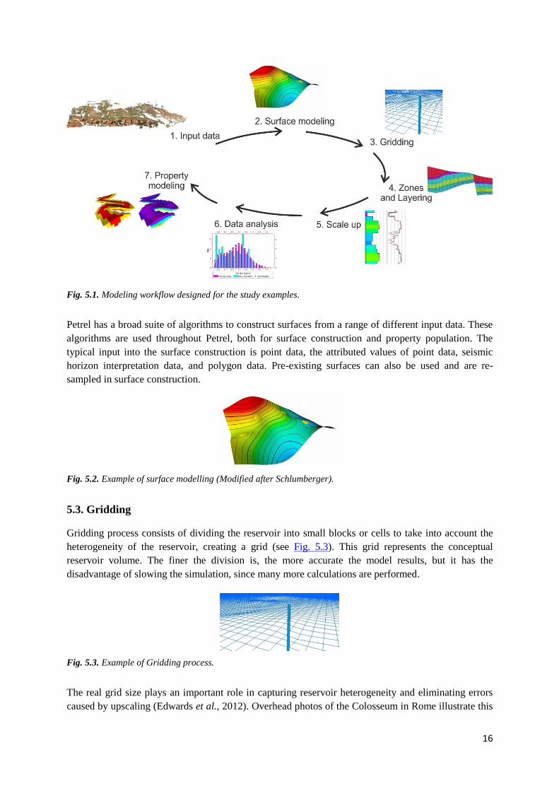
Fig. 5.1. Modeling workflow designed for the study examples.

Petrel has a broad suite of algorithms to construct surfaces from a range of different input data. These

algorithms are used throughout Petrel, both for surface construction and property population. The

typical input into the surface construction is point data, the attributed values of point data, seismic

horizon interpretation data, and polygon data. Pre-existing surfaces can also be used and are re-

sampled in surface construction.

Fig. 5.2. Example of surface modelling (Modified after Schlumberger).

5.3. Gridding

Gridding process consists of dividing the reservoir into small blocks or cells to take into account the

heterogeneity of the reservoir, creating a grid (see Fig. 5.3). This grid represents the conceptual

reservoir volume. The finer the division is, the more accurate the model results, but it has the

disadvantage of slowing the simulation, since many more calculations are performed.

Fig. 5.3. Example of Gridding process.

The real grid size plays an important role in capturing reservoir heterogeneity and eliminating errors

caused by upscaling (Edwards et al., 2012). Overhead photos of the Colosseum in Rome illustrate this

17

concept (see Fig 5.4). If the area of interest is the Colosseum floor, then a 50m x 50m grid will be

appropriated to capture what is required. Choice of a larger 250m x 250m grid includes driveways,

streets, landscaping and other features which are not associated with the focal point of interest. In the

case of the Colosseum, using a larger grid to capture properties associated with the floor would

introduce errors.

Fig. 5.4. Grid Resolution. Example of the Colosseum in Rome (Modified after Edwards et al., 2012).

The choice of grid and grid-cell dimensions is highly important. The upscaled of the permeability, the

balance of fluid forces, and the variance of a reservoir property are all intimately connected with the

length-scale model (Ringlose et al., 2015).

Therefore, the determination of the grid is one of the most important points to consider from the

beginning of the generation of a model and it will be conditioned by the time to use in the model. It is

advisable to use the simpler and coarser grid possible model, whose results are sufficiently reliable and

accurate to allow to take appropriate decisions.

5.4. Zones and Layering

Making Zones and Layering are the two last steps in defining the vertical resolution of the 3D grid

(see Fig. 5.5).

The Zones process is used when a geological zonation is available. Each zone is defined by two

surfaces.

The Layering process enables you to define the final vertical resolution of the grid by setting the

thickness of the cell or the number of desired cell layers. Layering is not defined by enclosing

surfaces. Layering is defined as the internal layering reflecting the geological deposition of a specific

zone. Layers only sub-divide the grid between the zone-related surfaces.

Fig. 5.5. Differences between Zones and Layering (Modified after Schlumberger).

18

5.5. Scale up

Scale up well logs is the process of sampling values from well logs or well log attributes into the grid,

ready for its use as input to both facies and petrophysical modeling.

When upscaling well logs, Petrel will first find the 3D grid cells which the wells penetrate (see Fig.

5.6 A). For each grid cell, all of the log values that fall within the cell will be averaged according to

the selected algorithm to produce one log value for that cell (see Fig. 5.6 B y C).

Fig. 5.6. A) Concept of Scale up. B) Example of Scale up in the wells. C) Example of Scale up in the logs

(Modified after Schlumberger).

In summary, the Scale up well logs process assigns log values to the cells in the 3D grid that are

penetrated by the wells. It is the first step towards the distribution of petrophysical properties values in

all cells of the model.

5.6. Data analysis

Data analysis is the process of preparing and controlling the quality of the input data (normally

upscaled well logs) for property modeling. It involves applying transformations on input data,

identifying trends for continuous data, vertical proportion, and probability for discrete data. It also

involves defining variograms that describe the input for both cases (see Fig. 5.7). Then it is used in the

facies and petrophysical modeling to ensure that the same trends appear in the result.

The Data analysis process enables a detailed analysis of both discrete and continuous properties. The

facies proportion, thickness, attribute probability, and variogram modeling are available for discrete

properties. Data transformations as well as modeling variograms are available for continuous

properties.

Fig. 5.7. Example of Data analysis (Modified after Schlumberger).

19

5.7. Property modeling: Facies and Petrophysical modeling

Property modeling is the process of filling the cells of the grid with discrete (facies) or continuous

(petrophysics) properties (see Fig. 5.8). Petrel assumes that the layer geometry given to the grid

follows the geological layering in the model area. Thus, these are processes which depend on the

geometry of the existing grid. When interpolating between data points, Petrel will propagate property

values along the grid layers.

Facies modeling is a means of distributing discrete data (e.g. facies) throughout the 3D model. In

Petrel, stochastic and deterministic methods are available for modeling the distribution of discrete

properties in a reservoir. The modeling inputs are the upscaled facies well logs, modeling parameters,

and possible trends within the reservoir (modeled in the Data analysis process).

Petrophysical modeling is the interpolation or simulation of continuous data (for example, porosity or

permeability) throughout the model grid. In Petrel Deterministic (estimation or interpolation) and

Stochastic methods are available for modeling the distribution of continuous properties in a reservoir

model. Well data, facies realization, variograms, a secondary variable and/or trend data can be used as

input. As usually, upscaled well logs data is the available set of data with continuous properties in the

model grid.

Fig. 5.8. Property modeling examples (Modified after Schlumberger).

5.8. Deterministic versus stochastic algorithms

The main division in the modeling algorithms available in Petrel is between Deterministic and

Stochastic methods. Both types of algorithms are available in the Facies modeling and Petrophysical

modeling processes.

The deterministic algorithms always give the same result with the same input data. Deterministic

algorithms are very transparent; it is easy to see why a particular cell has been given a particular value.

The disadvantage is that models with little input data will automatically be smooth even though

evidence and experience may suggest that this is not likely. Getting a good idea of the uncertainty of a

model away from the input data points is often difficult in such models.

The stochastic algorithms use a random seed in addition to the input data. Therefore, while

consecutive runs will give similar results with the same input data, the details of the results will be

different. The Stochastic algorithms such as Sequential Gaussian Simulation are complex and take

much more time to run than deterministic algorithms. However, they emphasize more notable aspects

of the input data, specifically the variability of the input data. This means that local highs and lows

will appear in the results that are not steered by the input data and whose location is purely an artefact

of the random seed used. The resulting distribution is more typical of the real case, although the

specific variation is unlikely to match. This can be particularly useful when taking the model further to

simulation, as the variability of a property is likely to be just as important as its average value. The

disadvantage is that some important aspects of the model can be random and it is important to perform

a proper uncertainty analysis with several realizations of the same property model with different

random seeds.

20

6. RESULTS

In this section the results obtained after modeling the two study examples are presented. It has been

followed the workflow described in the previous chapter. The comparison between a stochastic

modeling and a deterministic modeling is presented and each of the solutions obtained is assessed.

Finally, based on the obtained results, some ideas are given for exploiting these examples as analogous

reservoirs.

6.1. Zone A: Meandering System

As presented in Section 4.1, for this example we account with the following information as input data

for the model (see Fig 4.4): Data from outcrop with outstanding 3D features, data from 4 wells carried

out with the technique O/BO, 5 GPR lines that complete 3D subsurface information about the

sandstone geobody and finally, petrophysical data of porosity and permeability.

6.1.1. Surface modeling

For surfaces modeling, GPS data from outcrop, well tops defined in the wells and the information

provided by the GPR profiles have been taken as input data.

For the realization of the stochastic model, the bottom and top surfaces which limit the geobody are

modeled only (see Fig 6.1 A and B).

For modeling of the deterministic model, a more complex modeling of surface has been developed. It

has been also carried out, as well as the modeling the base and top surfaces which limit the body, the

modeling of surfaces bounding the main sub-environments within the body (see Fig. 6.1 C and D).

Based on this matter, the following areas have been modeled: bottom of the geobody, bottom of the

point bar, bottom of the channel and top of the body.

6.1.2. Model Characteristics

A grid of 4745 cells in the X and Y direction has been designed for this model. For the stochastic

model, including the vertical resolution, it has a total of 40000 cells. The deterministic model has a

total of 204 035 cells (see Table 6.1). Each cell has a dimension of 1m x 1m. We used the same design

grid for X and Y directions for both the stochastic model and the deterministic model. They only differ

in the vertical resolution of the grid, which is determined by the layering.

For the stochastic model a zone in the model bounded by the base surface and top model has been only

differentiated. 20 layers have been established for this model (see Table 6.1).

For the deterministic model we have differentiated 4 zones enclosed by the surfaces described above.

So we can distinguish the following areas: zone 1 which corresponds to contemporary floodplain to

the meandering body delimited by the bottom surface of model and the bottom point bar surface, zone

2 which corresponds to point bar, which is delimited by the bottom point bar surface and the bottom

surface of the channel, zone 3 corresponding to the channel, it is defined by the bottom channel

surface and the top channel surface, and finally, the zone 4 which corresponds to later floodplain them

meandering body which is delimited by the top channel surface and the top surface of the model. 43

layers for this model have been differentiated: 1 layer in the zone 1, 10 layers for zone 2, 31 layers for

zone 3 and 1 layer for zone 4 (see Table 6.1).

21

Fig. 6.1. Surfaces modeling for the meandering system study example. A and B) show the surface modeling for

stochastic method. C and D) show the surface modeling for deterministic method.

6.1.3. Scale up

In this process of preparing the data in order to entry them into the model, a first upscaling of the

lithofacies based on the previous study has been made. Lithofacies were grouped according to the

criteria of sub-environment to which they belong (see Fig. 6.2). Due to the problem that we wanted to

address, the first upscaling has been carried out to model and predict the distribution of the different

sub-environments previously distinguished in the geobody.

So three variables have been introduced to the model: Channel, Point bar and Flood plain.

In the case of upscaling of the petrophysical properties (porosity and permeability) the median of the

data has been performed as method of averaging the cell. The log has been treated as a line. The scale

up interpolation method used has been the neighbor cell. For this example these upscaling

characteristics are best suited to the input data (see Fig. 6.3).

Legend surfaces:

22

Table 6.1. Grid, zones and layers characteristics in the models of the meandering system.

Fig. 6.2. Lithofacies Scale up. In the right column it is shown the upscaling of lithofacies. In orange appears

channel, in yellow the point bar and in green the flood plain facies.

23

Fig. 6.3. Scale up of petrophysical data in wells MB3 and MB4. A) Facies logs. B and D) Porosity and

permeability logs. C and E) Result of upscaling.

6.1.4. Data analysis

In this process of analysis, preparation and quality control of data for subsequent modeling has been

performed. The quality control of the input data in both discrete data (facies) and for continuous data

(porosity and permeability) shows that the proportions of the input data are correct (see Fig 6.4).

Fig. 6.4. Data analysis of facies, porosity and permeability for the meandering system study example.

Then porosity and permeability data have been faced to find a relationship between these two

parameters (see Fig. 6.5), a quality control between the input data and upscaling data has been made

(see Fig. 6.6) and finally a variogram showing the relationship between both parameters, has been

generated (see Fig. 6.7) to be subsequently inserted in the petrophysical model.

24

Fig. 6.5. Cross plot of porosity versus permeability.

Quality control between input data of porosity and permeability and upscaled data shows that the

process of scale up has virtually taken into account all the input values.

In the process of searching for a variogram representing a correlation between the data deriving from

petrophysical parameters (porosity and permeability) has been determined that there is a fairly good

linear correlation between both parameters, showing a correlation coefficient of 0.83 (see Fig. 6.7).

This generated variogram has been introduced in the petrophysical model.

Fig. 6.6. Quality control between well logs and upscaled data.

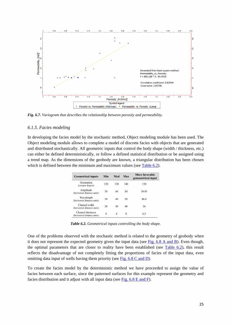
25

Fig. 6.7. Variogram that describes the relationship between porosity and permeability.

6.1.5. Facies modeling

In developing the facies model by the stochastic method, Object modeling module has been used. The

Object modeling module allows to complete a model of discrete facies with objects that are generated

and distributed stochastically. All geometric inputs that control the body shape (width / thickness, etc.)

can either be defined deterministically, or follow a defined statistical distribution or be assigned using

a trend map. As the dimensions of the geobody are known, a triangular distribution has been chosen

which is defined between the minimum and maximum values (see Table 6.2).

Table 6.2. Geometrical inputs controlling the body shape.

One of the problems observed with the stochastic method is related to the geometry of geobody when

it does not represent the expected geometry given the input data (see Fig. 6.8 A and B). Even though,

the optimal parameters that are closer to reality have been established (see Table 6.2), this result

reflects the disadvantage of not completely fitting the proportions of facies of the input data, even

omitting data input of wells having them priority (see Fig. 6.8 C and D).

To create the facies model by the deterministic method we have proceeded to assign the value of

facies between each surface, since the patterned surfaces for this example represent the geometry and

facies distribution and it adjust with all input data (see Fig. 6.8 E and F).

26

Fig. 6.8. Facies models. A-C) show the little geometric fit of facies models generated by stochastic methods. D)

shows how these examples above did not conform fully to the input data of wells. E) represents the facies model

generated deterministically. F) shows how the deterministic facies model is adjusted to the input data. The

legend of all figures is represented in figure F on the upper right margin.

Quality control of deterministic model considered on the selection of a section from the model that

corresponds to the outcropping part of the geobody and to check if that model meets the reality. From

Figure 6.9, it is seen that the model perfectly fits the geometry interpreted in outcrop.

Fig. 6.9. Quality control of the deterministic model with outcrop. For the legend of the colors see Fig. 6.8 F.

27

6.1.6. Petrophysical modeling

The petrophysical modeling of porosity and permeability was performed using sequential gaussian

simulation. The sequential gaussian simulation is a stochastic method based on kriging interpolation.

This method can honor input data, input distributions, variograms and trends. For this reason mainly,

this method has been chosen.

During the simulation, local highs and lows will be generated between input data locations which

honor the variogram. The positions of these highs and lows will be determined by a random number

supplied by the user or the software. These maximum and minimum values have been attributed based

on laboratory data presented at the section of data acquisition. The results generated will not give

values above the maximum or below the minimum of the input data.

As variogram input for the simulation has been introduced the generated variogram for this example

shown in section 6.1.4. Data analysis.

The results of both porosity and permeability, faithfully reflect the expected solution by stochastic

methods (see Fig 6.10). They present higher values of porosity and permeability in the margin of the

channel and in the scroll bar.

It should be noted that the generated petrophysical models are closely related with the generated facies

model. Therefore, the spatial variation of the generated petrophysical properties by stochastic methods

faithfully corresponds to reality although its distribution is linked to the previously generated facies

model, which has been made by deterministic methods, as shown in section 6.1.5.

Fig. 6.10. Porosity and Permeability models. On the left the 3D porosity model is displayed (A) and its testing

with the outcrop section (B). On the right the 3D permeability model is displayed (C) and its testing with the

outcrop section (D).

6.1.7. Operations strategy

Based on the results of the derived models, potential drilling strategies are proposed for operational of

this outcrop analog example. The first design that is outlined raises vertical wells located mainly in

areas of the scroll bar and the zone of the channel margin, since these areas are those with higher

permeability values (see Fig. 6.11 A). Another outlined design consists of wells deviated that target

channel margin zone and the whole zone of the point bar until the scroll bar (see Fig. 6.11 B). Finally,

28

there is an intermediate outline between the two previous designs which consists of the horizontal

drilling following the channel talweg by cutting it at its margins (see Fig. 6.11 C). This latest proposal

is ideal but very difficult to be executed in these systems due to the high variability in the direction

that are presented by high sinuosity meandering systems.

Fig. 6.11. Wells design for the exploiting strategy of this study example as outcrop analog. A) shows the design

of vertical boreholes. B) shows the design of deviated boreholes. C) shows the design of horizontal boreholes.

6.2. Zone B: Braided System

As presented in the above section (section 4.2), for this study example the following previous

information has been used as input data in the model (see Fig 4.4): Data from outcrop with outstanding

3D features, data from 6 wells with all information collected in the previous points, 4 lines of GPR

that complete 3D information of the body under study and finally, porosity and permeability

petrophysical data.

6.2.1. Surface modeling

For surfaces modeling in this example, the data taken with GPS on outcrop and well tops defined in

the well have been taken as input.

The same as in the meandering example, for the realization of the stochastic model only the bottom

and top sufaces that limit the geobody are modeled (see Fig 6.12 A and B).

For modeling of deterministic model, in addition to the modeling of the base and top surfaces which

limit the body, the modeling of surfaces that bounds the sub-environment of the channels that are

observed in the input data have been carried out too (see Fig. 6.12 C and D). On this basis, the

following surfaces have been modeled: bottom of the geobody, bottom of the two channels and top of

the body.

29

Fig. 6.12. Surfaces modeling for the braided system study example. A and B) show the surface modeling for

stochastic method. C and D) show the surface modeling for deterministic method.

6.2.2. Model Characteristics

For this model a grid that has 66443 cells in the X and Y direction has been designed. For the

stochastic model, including the vertical resolution, it has a total of 1993290 cells. The deterministic

model has a total of 4983225 cells (see Table 6.3). Each cell has a dimension of 5m x 5m. We used the

same design grid for X and Y directions for both the stochastic and the deterministic model, they only

differ in the vertical resolution of the grid, which is determined by the layering.

For the stochastic model a zone in the model bounded by the base surface and top model has been only

differentiated. 30 layers have been differentiated for this model (see Table 6.3).

For the deterministic model there are 2 differentiated zones enclosed by surfaces described above. So

we can distinguish the following areas: zone 1 which corresponds to the compound bar delimited by

the bottom surface of model and the bottom channels surface and zone 2 which corresponds to

channels, it is delimited by the bottom channels surface and the top surface of the model. It has been

differentiated 75 layers for this model: 29 layers in the zone 1 and 46 layers for zone 2 (see Table 6.3).

30

Table 6.3. Grid, zones and layers characteristics of the models of the braided system.

6.2.3. Scale up

In this process of preparing the data for their entry into the model a first upscaling of the lithofacies

based on the previous study has been made. Lithofacies were grouped according to the criteria of sub-

environment to which they belong (see Fig. 6.13). It has chosen to undertake this first upscaling due to

the problem that we wanted to address, to model and predict the distribution of the different sub-

environments of the geobody.

So, two variables have been introduced to the model: Channel and Compound bar.

In the upscaling of the petrophysical properties (porosity and permeability) the arithmetic of the data

as method of averaging the cell has been carried out. The log has been treated as a line. The scale up

interpolation method used has been the neighbor cell. For this example these upscaling characteristics

are best suited to the input data (see Fig. 6.14).

31

Fig. 6.13. Lithofacies Scale up for the braided system example. In the right column it is shown the upscaling of

lithofacies. The channel appears in orange and in yellow the compound bar.

Fig. 6.14. Scale up of petrophysical data in wells K2P1 and K2P2. A) Facies logs. B and D) Porosity and

permeability logs. C and E) Result of upscaling.

32

6.2.4. Data analysis

The quality control of the input data in both discrete data (facies) and continuous data (porosity and

permeability) have been performed in the first place, testing that the proportions of the input data are

correct (see Fig 6.15).

Fig. 6.15. Data analysis of facies, porosity and permeability.

Then porosity and permeability data have been faced to find a relationship between these two

parameters (see Fig. 6.16), a quality control between the input data and upscaling data has been made

(see Fig. 6.17) and finally, it has been generated a variogram showing the relationship between both

parameters (see Fig. 6.18) and then insert it in the petrophysical model.

Fig. 6.16. Cross plot of porosity versus permeability.

In the quality control of input data between porosity and permeability and upscaled data it has been

proved that the scale up process has taken into account almost all input values.

The variogram representing the correlation between petrophysical parameters of porosity and

permeability has determined that there is a fairly good linear correlation between both parameters,

showing a correlation coefficient of 0.89 (see Fig. 6.18). This generated variogram has been

introduced in the petrophysical model.

33

Fig. 6.17. Quality control between well logs and upscaled data.

Fig. 6.18. Variogram that describes the relationship between porosity and permeability.

6.2.5. Facies modeling

In developing of the facies model for the stochastic method it has been used Object modeling module,

as in the previous example. As the geobody dimensions are known also a triangular distribution has

been chosen (see Table 6.4).

Table 6.4. Geometrical inputs controlling the body shape.

34

In this example we find the same problems as in the example above concerning stochastic models:

poor geometry, ignore input wells and imbalance in the proportions of facies of the input data.

Furthermore we must add the poor affinity of the resulting geometries with reality (see Fig. 6.19 A, B

and C). Besides we have to add an important problem to predict the spatial distribution of some facies

or sub-environments.

To create the facies model by the deterministic method we have proceeded to assign the value of

facies between each surface, following the same procedure as the previous example (see Fig. 6.19 D

and E).

Fig. 6.19. Facies model. A-C) show the little geometric fit of facies models generated by stochastic methods. D)

shows how the deterministic facies model is adjusted to the input data (outcrop). E) represents the facies model

generated deterministically. On its lower left margin the legend is presented.

35

As the previous example, with the purpose of perform quality control of the deterministic model a

section of the model that corresponds to the section of outcrop has been selected and it has faced to

check whether the model meets reality (see Fig. 6.20). It can be seen that the model responds perfectly

to the geometry interpreted in outcrop also in this example.

Fig. 6.20. Quality control of the deterministic model with outcrop. For the legend of the colors see Fig. 6.19 E.

6.2.6. Petrophysical modeling

In the petrophysical modeling of porosity and permeability a sequential gaussian simulation has been

also chosen for this example.

As input variogram for the simulation the variogram generated for this example shown in section

6.2.4. has been introduced.

The results of both porosity and permeability, faithfully reflect the expected solution by stochastic

methods (see Fig. 6.21). They present higher values of porosity and permeability in the channel.

Like the previous example, the generated petrophysical models are closely related with the facies

generated model.

Fig. 6.21. Porosity and Permeability models for the braided system study example. On the left the 3D porosity

model (A) and its testing with the outcrop section (B) are displayed. On the right the 3D permeability model (C)

and its testing with the outcrop section (D) are shown.

6.2.7. Operations strategy

According to the results of the obtained models possible designs of drilling are proposed for

operational of this outcrop analog example. The first design that is outlined consists of vertical wells

36

located mainly in the channels, as these zones are those with the highest permeability, and in the

center of the compound bar, to prevent the permeability barrier laterally presented in these bodies, as it

can be seen in the resulting models (see Fig. 6.22 A). The second design that is outlined consists of

horizontal drilling in the channels and following the trend of these (see Fig. 6.22 B). Finally, a design

is also planted combining the two techniques: vertical wells in the centers of the compound bar and

horizontal wells in the channels following the trend they present (see Fig 6.22 C).

Fig. 6.22. Wells design for the exploiting strategy of this study example as outcrop analog. A) shows the design

of vertical boreholes. B) shows the design of horizontal boreholes. C) shows the design of boreholes combining

previous designs (A and B).

7. CONCLUSIONS

3D modeling of the study examples interpreted as a meandering and a braided fluvial systems based

upon the geometry of the differentiated sub-environments, their lithofacies distribution and their

corresponding subsurface data from wells and well logs as well as various GPR profiles brings us to

the following conclusions:

- The elements producing sedimentary heterogeneity recognized in outcrop for the meandering system

example correspond to the sub-environments of the main channel, point bar, scroll bar and chute

channel. For the braided system example, the main sedimentary heterogeneity is due to the distribution

of channel and compound bar sub-environments.

- This work shows that addressing the modeling of the geometry of reservoirs in sandstone geobodies

of fluvial origin of the type studied, the dimensions to be estimated in transverse cross section are

between 10 and 1000 m for meandering systems and between 100 and 10000 m for braided systems.

Similarly, the maximum thickness to meandering geobodies is of order metric to decametric, while for

braided sandstone units is in the order of hundred meters.

- The multi-scale approach of this study and its implementation in the static model have shown most

of the heterogeneities observed at the macro, meso and micro scale, assuming a significant advantage

over typical homogeneous static models. The determination of heterogeneities and its full integration

into a static model of reservoir leads to greater quantitative accuracy when using the model for the

potential exploitation of the resources accumulated in the rock.

37

- The models which are made by stochastic methods have not failed to reproduce facies

heterogeneities since they have not shown the precise geometry of architectural elements and

appropriate facies distribution and do not respect the proportion of facies introduced by the wells,

which are the control point in the model. However, the stochastic models have faithfully reproduced

the petrophysical heterogeneities of porosity and permeability in both examples.

- The modeling strategy designed for the deterministic models has allowed showing heterogeneity in

the distribution of facies, getting a very high approximation to the data observed in outcrop.

- The obtained model clearly reflects how higher porosity and permeability values are associated with

the margin channel and scroll bar facies in the meandering system study case, thus confirming the

existence of a large sedimentary control over the petrophysical heterogeneity in the geobody. The

model for braided system example presents more homogeneous porosity and permeability values in its

totality, being channel sub-environment which presents more favorable petrophysical properties.

- In general, the braided system geobody can be considered of more interest in regards to exploitation

as reservoir, considering that it has larger dimensions than the meandering system unit and more

favorable petrophysical properties. Moreover, the operational design in such analogs is much simpler

than in meandering system.

CONCLUSIONES

La modelización 3D de los ejemplos objetos de estudio interpretados como un sistema fluvial

meandriforme y un sistema fluvial trenzado a partir de la geometría de los subambientes diferenciados,

sus correspondientes litofacies y los datos de subsuelo procedentes de sondeos y sus diagrafías y

varios perfiles de GPR nos conduce a las siguientes conclusiones:

- Los elementos que producen heterogeneidad sedimentaria reconocidos en afloramiento para el

sistema meandriforme se corresponden con los subambientes de canal principal, point bar, scroll bar y

canal de chute. Para el sistema trenzado se corresponden con los subambientes de canal y barra

compuesta.

- Se pone de manifiesto que a la hora de abordar la modelización de la geometría de reservorios en

cuerpos de arenisca de origen fluvial del tipo de los estudiados, las dimensiones que deben estimarse

en sección transversal están entre 10 y 1000 m para sistemas meandriformes y entre 100 y 10000 m

para sistemas trenzados. Del mismo modo, el espesor máximo para cuerpos del sistema meandriforme

es de orden métrico a decamétrico, mientras que para areniscas del sistema trenzado se sitúa en el

orden del centenar de metros.

- El estudio integrado a multi-escala y su implementación en el modelo estático ha reproducido la

mayor parte de las heterogeneidades que se observan a macro, meso y micro escala, suponiendo una

notable ventaja frente a los típicos modelos estáticos homogéneos. La determinación de las

heterogeneidades y su integración absoluta en un modelo estático del reservorio conduce a una mayor

precisión cuantitativa, a la hora de utilizar el modelo para la potencial explotación de los recursos

almacenados en la roca.

- Los modelos realizados por métodos estocásticos no han permitido reproducir las heterogeneidades

de facies ya que no han representado la geometría y distribución adecuada de las facies ni respeta la

proporción de facies introducida por los sondeos, que son el punto de control en el modelo. Sin

38

embargo, los modelos estocásticos si han reproducido fielmente las heterogeneidades petrofísicas de

porosidad y permeabilidad en ambos ejemplos.

- La estrategia de modelización diseñada para los modelos determinísticos ha permitido reproducir la

heterogeneidad en la distribución de facies, obteniéndose una aproximación muy alta a los datos

observados en afloramiento.

- El modelo refleja con claridad cómo los valores más altos de porosidad y permeabilidad se asocian a

las facies de margen de canal y de scroll bar, para el sistema meandriforme, confirmándose por tanto

la existencia de un importante control sedimentario sobre la heterogeneidad petrofísica en la capa

estudiada. El modelo del sistema trenzado presenta unos valores más homogéneos de porosidad y

permeabilidad en toda su extensión, siendo el subambiente de canal el que mejores propiedades

petrofísicas presenta.

- El sistema trenzado presenta mayor interés de cara a la explotación como reservorio, ya que además

de tener unas dimensiones mucho mayores que el sistema meandriforme presenta unas propiedades

petrofísicas idóneas. El diseño de explotación en este tipo de análogos es mucho más sencilla que en el

caso del ejemplo meandriforme.

8. REFERENCES

Abatan, O.; Kerr, D. and Ramachandran, K. (2013).

Meandering Channel Facies Architecture Using

Ground Penetrating Radar, Ferron Sandstone

(Upper Cretaceous) Emery Co., Utah. AAPG

Search and Discovery Article #41134.

Alexander, J. (1992). A discussion on the use of

analogues for reservoir geology. Geological

Society of London 69(1): 175-194.

Arche, A.; López-Gómez, J and García-Hidalgo, J.

F. (2002). Control climático, tectónico y

eustático en depósitos del Carniense (Triásico

Superior) del SE de la Península Ibérica.

Journal of Iberian Geology, 28, 13-30.

Ashmore, P. (1982). Laboratory modeling of gravel

braided stream morphology. Earth Surface

Processes and Landforms 7, 201-225.

Beidinger, A.; Decker, K. and Roch, K. H. (2011).

The Lassee segment of the Vienna Basin fault

system as a potential source of the earthquake of

Carnuntum in the fourth century A.D. Springer,

Int. J. Earth Sci. (Geol Rundsch) 100:1315–

1329.

Bourquin, S. ; Guillocheau, F. and Péron, S. (2009).

Braided rivers within an arid alluvial plain

(example from the Lower Triassic, western

German Basin): recognition criteria and

expression of stratigraphic cycles.

Sedimentology (2009) 56, 2235–2264.

Bryant, I.; Carr, D.; Cirilli, P.; Drink N.;

McCormick, D.; Tilke, P. and Thurmond, J.

(2000). Use of 3D digital analogues as

templates in reservoir modeling. Petroleum

Geoscience 6(3): 195-201.

Cabello, P.; López-Blanco, M.; Falivene, O.;

Arbués, P.; Ramos, E.; Cabrera, Ll. and Marzo,

M (2006). Modelos 3D de análogos de

reservorios sedimentarios: Aplicación al sistema

de abanico costero eoceno de Sant Llorenç del

Munt (Cuenca del Ebro). Geo-Temas 9.

Calvache, M. L.; Fernández, J.; García-García, F.;

Soria, J. M. and Viseras, C. (2010). From the

Geomorphic Process to Basin Architecture:

Anatomy of the Infill of an Alluvial-Lacustrine

System in Southern Spain. The Open Geology

Journal, 2010, 4, 86-104.

Cant, D.J. and Walker, R.G. (1978). Fluvial

processes and facies sequences in the sandy

braided South Saskatchewan River, Canada.

Sedimentology 25, 625-648.

Corbeanu, R. M.; Soegaard, K.; Szerbiak, R. B.;

Thurmond, J. B.; McMechan, G. A.; Wang, D.;

Snelgrove, S.; Forster, C. B.and Menitove, A.

(2001). Detailed internal architecture of a fluvial

channel sandstone determined from outcrop,

cores, and 3-D ground-penetrating radar:

Example from the middle Cretaceous Ferron

Sandstone, east-central Utah. AAPG Bulletin, v.

85, no. 9 (September 2001), pp. 1583–1608.

Critelli, S.; Mongelli, G.; Perri, F.; Martín-Algarra,

A.; Martín-Martín, M.; Perrone, V.; Dominici,

R.; Sonnino, M. and Najib Zaghloul, M. (2008).

Compositional and Geochemical Signatures for

the Sedimentary Evolution of the Middle

39

Triassic–Lower Jurassic Continental Redbeds

from Western-Central Mediterranean Alpine

Chains. The Journal of Geology, 2008, volume

116, p. 375–386.

Edwards, D. A.; Gunasekera, D.; Morris, J.; Shaw,

G.; Shaw, K. and Walsh, D. (2012). Reservoir

simulation: Keeping Pace with Oilfield

Complexity. Oilfield Review.

Dabrio, C.J. and Fernández, J. (1986). Evolución

del estilo aluvial en el Triásico de Alcaraz

(Albacete). Cuad. Geol. Ibérica,10: 173-206.

Dodge, C. F.; Holler, D. P. and Meyer, R. L.

(1971). Reservoir Heterogenetities of Some

Cretaceous Sandstones: AAPG Bulletin, v. 55,

no. 10, p. 1814-1820.

Enge, H. D.; Buckley, S. J.; Rotevatn, A. and

Howell, J. A. (2007). From outcrop to reservoir

simulation model: Workflow and procedures.

Geosphere 3(6): 469-490.

Fernández, J. (1977). Sedimentación triásica en el

borde SE de la Meseta. Tesis Univ. Granada,

173 págs.

Fernández, J. (1984). Capas rojas triásicas del borde

Sureste de la Meseta, síntesis estratigráfica y

sedimentológica. Mediterránea, 3: 89-105.

Fernández, J. and Dabrio, C.J. (1985). Fluvial

architecture of the Buntsandstein facies red beds

in the Middle to Upper Triassic (Ladinian-

Norian) of the Southeastern edge of the Iberian

Meseta (Southern Spain). Aspects of fluvial

sedimentation in the Lower Triassic

Buntsandstein of Europe (D. Mader. ed.).

Lectures Notes in Earth Sciences. Springer-

Verlag, 4: 411-435.

Fernández, J. and Gil, A. (1989). Interpretación

sedimentaria de los materiales triásicos de facies

Buntsandstein en las zonas Externas de las

Cordilleras Béticas, y en la Cobertera Tabular

de la Meseta. Rev. Soc. Geol. España,2: 113-

124.

Fernández, J.; Dabrio, C..J. and Pérez López, A.

(1993). El Triásico de la región de Siles-

Alcaraz. Gráficas Cuenca, 47 págs.

Fernández, J.; Dabrio, C..J. and Pérez López, A.

(1994). El Triásico de la región de Siles-

Alcaraz. Gráficas Cuenca, 47 págs.

Fernández, J.; Dabrio, C.J. and Viseras, C. (2005).

Triassic fluvial sandstones (Central South

Spain). An excellent Analogue for the TAGI

reservoir of Algeria. 67th EAGE Conference

and Exhibition, Field trip 1 guide.

Franke, D.; Hornung, J. and Hinderer, M. (2015). A

combined study of radar facies, lithofacies and

three-dimensional architecture of an alpine

alluvial fan (Illgraben fan, Switzerland).

Sedimentology (2015) 62, 57–86.

Gay, S.P. (1989). Gravitational compaction, a

neglected mechanism in structural and

stratigraphic studies: new evidences from

Midcontinent, USA. AAPG Bulletin, 73: 641-

657.

Goy, A. and Yébenes, A. 1977. Características,

extensión y edad de la formación Dolomías

tableadas de Imón. Cuadernos de Geología

Ibérica, 4, 375-384.

Haq, B. U.; Hardenbol, J. and Vail, P.R. (1987).

Chronology of fluctuating sea levels since the

Triassic. Science, 235: 1156-1167.

Henares, S. (2011). Estudio petrológico y

petrofísico en las capas rojas triásicas de la

Cobertera Tabular de la Meseta Ibérica (Sector

de Alcaraz). Máster, Universidad de Granada,

Granada, 73 p.

Henares, S.; Caracciolo, L.; Cultrone, G.;

Fernández, J.; Viseras, C. (2014). The role of

diagénesis and depositional facies on pore

system evolution in a Triassic outcrop analogue

(SE Spain). Marine and Petroleum Geology 51,

136-151.

Henares, S.; Caracciolo L.; Viseras C.; Yeste, L.

M.; Fernández, J. (2015). Pore-scale

heterogeneity in meandering fluvial reservoirs: a

Triassic outcrop analogue. 77th EAGE

Conference & Exhibition 2015. Madrid IFEMA,

Spain, 1-4 June 2015.

Hugenholtz, C. H.; Paulen, R.C. and Wolfe S.A.

(2007). Ground-penetrating-radar investigation

of relict channel bars of the Meander River

spillway, northern Alberta. Geological Survey of

Canada, Current Research 2007-A1, 10 p.

Hutchinson, J. R.; C. F. Dodge and T. L. olasek

(1961). Identification, classification and

prediction of reservoir nonuniformities affecting

production operations. Journal of Petroleum

Technology, v. 13, p. 223-230.

Jorry, S. J. and Biévre, G. (2011). Integration of

sedimentology and ground-penetrating radar for

high-resolution imaging of a carbonate

platform. Sedimentology (2011) 58, 1370–1390.

Keogh, K. (2007). Sequence stratigraphy and 3-D

modelling of the East Pennine Coalfield, UK: a

deterministic and stochastic approach, PhD,

University of Liverpool, UK.

Kostic B. and Aigner T. (2007). Sedimentary

architecture and 3D ground-penetrating radar

analysis of gravelly meandering river deposits

(Neckar Valley, SW Germany). Sedimentology

(2007) 54, 789–808.

40

Miall, A. 1996. The Geology of Fluvial Deposits.

Sedimentary Facies, Basin Analysis, and

Petroleum Geology. Springer eds. 582 p.

Nielsen, L.; Brockdorff, A. S. V.; Bjerager, M. and

Surlyk, F. (2009). Three-dimensional

architecture and development of Danian

bryozoan mounds at Limhamn, south-west

Sweden, using ground-penetrating radar.

Sedimentology (2009) 56, 695–708.

López Garrido, A.C. 1971. Geología de la Zona

Prebética al NE de la Provincia de Jaén. Tesis

doctoral, Universidad de Granada, 371 pp.

Lunt, Ian; Sambrook A.; Smith, G. Best, H.; Philip,

James L.; Ashworth, J.; Lane, S. N. and

Simpson, Christopher J. (2013). Deposits of the

sandy braided South Saskatchewan River:

Implications for the use of modern analogs in

reconstructing channel dimensions in reservoir

characterization. AAPG Bulletin, v. 97, no. 4

(April 2013), pp. 553–576.

Pascucci, V.; Peter Martini; I. and Endres; A. L.

(2009). Facies and ground-penetrating radar

characteristics of coarse-grained beach deposits

of the uppermost Pleistocene glacial Lake

Algonquin, Ontario, Canada. Sedimentology

(2009) 56, 529–545.

Pérez López A.; Solé de Porta N.; Márquez, L. and

Márquez Aliaga, A. (1992). Caracterización y

datación de una unidad carbonática de edad

Noriense (Formación Zamoranos) en el Trías de

la Zona Subbética. Rev. Soc. Geol. de España,

5: 113-127.

Pringle, J. K.; Howell, J. A. and Hodgetts, D.

(2006). Virtual outcrop models of petroleum

reservoir analogues: a review of the current

state-of-the-art. Firts Break, v. 24, p. 33-42.

Reesink, A. J. H.; Ashwortk, P. J.; Sambrook

Smith, G. H.; Best, J. L.; Parsons, D. R.;

Amsler, M. L.; Hardy, R. J.; Lane, Nicholas, S.

N, A. P.; Orfeo,O.; Sandbach, S. D.; Simpson,

C. J. and Szupiany, R. N. (2014). Scales and

causes of heterogeneity in bars in a large multi-

channel river: Río Panamá, Argentina.

Sedimentology (2014) 61, 1055–1085.

Rice,S. P.; Church, M.; Wooldridge, C. L. and

Hickin, E. J. (2009). Morphology and evolution

of bars in a wandering gravel-bed river; lower

Fraser river, British Columbia, Canada.

Sedimentology (2009) 56, 709–736.

Ringlose, P. and Bentley, M., (2015). Reservoir

model design. A practitioner’s guide. Springer.

Sánchez-Moya, Y.; Arribas, J.; Gómez-Gras, D.;

Marzo, M.; Pérez-Arlucea, M.; Sopeña, A.

(2004). Primera fase de rifting intracontinental

Pérmico Superior-Triásico. In: Vera, J.A. (Ed.),

Geología de España. SGE-IGME, Madrid, pp.

484-485.

Schlumberger (2015). Help Center of Petrel.

Słowik M. (2011). Reconstructing migration phases

of meandering channels by means of ground-

penetrating radar (GPR): the case of the Obra

River, Poland. Springer J Soils Sediments

(2011) 11:1262–1278.

Szerbiak, R. B.; McMechan, G. A.; Corbeanu, R.;

Forster, C. and Snelgrove, S. H. (2010). 3-D

characterization of a clastic reservoir analog:

From 3-D GPR data to a 3-D fluid permeability

model. Geophysics, Vol. 66, No. 4 (July-August

2001); P. 1026–1037.

Van Den Bril, K.; Gregoire, C.; Swennen, R. and

Lambot, S. (2007). Ground-penetrating radar as

a tool to detect rock heterogeneities (channels,

cemented layers and fractures) in the

Luxembourg Sandstone Formation (Grand-

Duchy of Luxembourg). Sedimentology (2007)

54, 949–967.

Viseras C. and Fernández, J. (1994). Channel

migration patterns and related sequences in

some alluvial fan systems. Sedimentary

Geology, 88, 201-217.

Viseras, C. and Fernández, J. (2010). Triassic

braidplain deposits and their potential

asreservoir rocks. Examples from Spain and

Morocco. In: Schwarz, E., Georgieff,

S.,Piovano, E., Ariztegui, D. (Eds.),

Sedimentology at the Foot on the Andes,

18th

International Sedimentological Congress,

Mendoza, Argentina, p. 908.

Viseras, C., Fernández, J., Henares, S., Cuellar, N.,

2011. Facies architecture in outcropping

analogues for the TAGI reservoir. Exploratory

interest. AAPG Search and Discovery Article

#90135, AAPG International Coference and

Exhibition, Milan, Italia.

Yeste, L.M.; Henares, S.; Fernández, J.; Teixidó,

T.; Peña, J.A. and Viseras, C. (2014).

Geomodelización 3D de análogos aflorantes de

reservorios sedimentarios: Un ejemplo triásico.

Geogaceta, 2014, 57, 95-98 .

Zeng, X.; McMechan, G. A.; Bhattacharya, J. P.;

Aiken, C. L.V.; Xu, X.; Hammon III, W. S. and

Corbeanu, R. M. (2004). 3D imaging of a

reservoir analogue in point bar deposits in the

Ferron Sandstone, Utah, using GPR.

Geophysical Prospecting, 2004, 52, 151-163.

I

APPENDIX I. LITHOFACIES TABLE

Facies

type Cod

Texture

And

Fabric

Sedimentary

structures and

Characteristics

Main process Environment Example

Gra

vel

ly

Gh · Granule-pebb.

· Clast supp.

· Weak horizontal

bedding

· Erosional base

· Weak clast

imbrication

· (*) Normal

grading

· (*) Inverse grading

· (*) High

proportion of

discoidal clasts

· High energy

traction

current

· Base of channel

· Base of point bar unit

· Head of lateral unit

bar

San

dy

Sm · Fine to medium

sand

· Massive

· Poorly imbr. mud

clasts

· (*) Weak

horizontal

bedding

· (*) Charcoal

fragments

· (*) Mud filled

fractures

· Channel fill

due to

waning flow

· (*) Bioturb.

· Channel pool

· Distal crevasse lobe

· Abandon channel

Sh · Fine to medium

sand

· Horizontal

lamination

· Parting lamination

· (*) Low angle

cross

lamination

· Sheetflow

· Point bar (lower and

upper parts of lateral

accretion units)

· Overbank (proximal to

channel)

· Riffle of braided

channel

Sp · Very fine to

coarse sand

· Planar cross

bedding

· Megarriple

migration

· Channel

· Compound bar

· Point bar (intermediate

part of lateral accretion

unit)

· Crevasse channel/lobe

Sps · Fine to coarse

sand

· Planar cross

bedding

· Asymptotic toe

· Mica/charcoal

fragments

accumulation at the

lower

part

· (*) Overlying

isolated

counter current

ripples

· Downstr.

migration of

braid bar

under high

water column

· Tail of braided bar

St

· Medium to

coarse sand

· (*) Granule

· Trough cross

bedding

· Pyrite nodules

concentrated at the

base

of troughs

· (*) Mud chips

lining the

cross beds

· Migrat. of

megarriples

and dunes

· Channel fill

· Channel · Overland rill

Appendix I.1. Simple lithofacies distinguished in the core.

II

Facies

type Cod

Texture

And

Fabric

Sedimentary

structures and

Characteristics

Main process Environment Example

San

dy

Sr · Very fine to

fine sand

· Current ripple

lamination

· (*) Flaser

lamination

· Migration of

current

ripples

· Crevasse lobe

(intermediate part)

· Flood Plain proximal

to

channel

· Slough channel

· Cross bar channel

Src · Very fine to

fine sand

· Asymmetric

climbing

ripple lamination

· Combin. of

traction and

settling from

suspension

· Crevasse lobe

· Straight channel

Srw

· Very fine sand

(occasionally

silt)

· Wave ripple

lamination

· Oscillatory

flow in a

standing

body of

water

· Lake/pond on the

floodplain

· Lagoon

· Abandon channel

· Straight channel

Slp · Very fine to

fine sand

· Low angle planar

cross bedding

·Migration of

ripples on the

channel bottom

and lateral

accretion surfaces

·Point bar

· Meandering channel

Lu

titi

c

Fr · Clay (rarely silt)

· Nodular

· Massive

· Slickensides

· Abundant rizoliths

· (*) Carbonate

nodules

· (*) Isolated silty

linsen

· (*) Stratiform

mottling

· (*) Spot mottling

· Soil develop.

on former

overbank

fines

· Flood plain (distal to

channel)

Fl · Clay and silt

· Horizontal

lamination

(lower flow regime)

· Uneven lamination

· Settling

from

suspension

· Mud drape over lateral

accretion units

· Swell depressions in

upper point bars

· Mud drape separating

phases of crevasse lobe

construction

· Clay plug in abandon

channel de derrame

Fll · Clay and silt

· Horizontal

lamination of

lower flow regime

· Isolated silty

linsen

· Settling

from

suspension

alternating

with tractive

episodes

· Channel in progressive

abandonment

(*) occasional appearance

Appendix I.1. Simple lithofacies distinguished in the core. (Cont.).

III

APPENDIX II. COMPOSITE WELL LOGS

Appendix II.1. Legend for composite well logs.

LEGEND

IV

Appendix II.2. Composite well log MB1.

V

Appendix II.3. Composite well log MB2.

VI

Appendix II.4. Composite well log MB3.

VII

Appendix II.5. Composite well log MB4.

VIII

Appendix II.6. Composite well log K2P1.

IX

Appendix II.7. Composite well log K2P2.

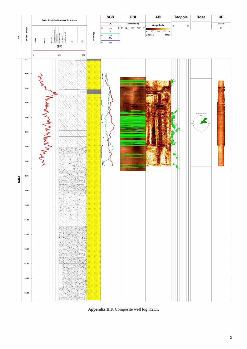
X

Appendix II.8. Composite well log K2L1.

XI

Appendix II.9. Composite well log K2L2.

XII

Appendix II.10. Composite well log K2L3.

XIII

Appendix II.11. Composite well log K2L4.

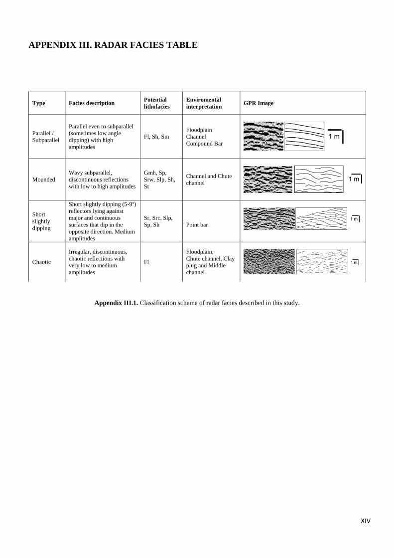
XIV

APPENDIX III. RADAR FACIES TABLE

Appendix III.1. Classification scheme of radar facies described in this study.

Type Facies description Potential

lithofacies

Enviromental

interpretation GPR Image

Parallel /

Subparallel

Parallel even to subparallel

(sometimes low angle

dipping) with high

amplitudes

Fl, Sh, Sm

Floodplain

Channel

Compound Bar

Mounded

Wavy subparallel,

discontinuous reflections

with low to high amplitudes

Gmh, Sp,

Srw, Slp, Sh,

St

Channel and Chute

channel

Short

slightly

dipping

Short slightly dipping (5-9º)

reflectors lying against

major and continuous

surfaces that dip in the

opposite direction. Medium

amplitudes

Sr, Src, Slp,

Sp, Sh

Point bar

Chaotic

Irregular, discontinuous,

chaotic reflections with

very low to medium

amplitudes

Fl

Floodplain,

Chute channel, Clay

plug and Middle

channel

XV

APPENDIX IV. GPR PROFILES

Appendix IV.1. GPR profile Bart-1.

XVI

Appendix IV.2. GPR profile Bart-2 and Bart-3.

XVII

Appendix IV.3. GPR profile Bart-4.

XVIII

Appendix IV.4. GPR profile Bart-5.

XIX

Appendix IV.5. GPR profile K2S-PR1

XX

Appendix IV.6. GPR profile K2S-PR2.

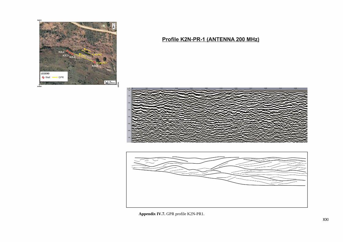
XXI

Appendix IV.7. GPR profile K2N-PR1.

XXII

Appendix IV.8. GPR profile K2N-PR2.