Zouhri-Final Report

1

Stress Analysis of a Chicago Electric 4½ Angle Grinder

By

Khalid Zouhri

A Project Submitted to the Graduate

Faculty of Rensselaer Polytechnic Institute

In Partial Fulfillment of the

Requirements for the degree of

MASTER OF MECHANICAL ENGINEERING

Approved:

_________________________________________

Dr.Ernesto Gutierrez-Miravete, Project Adviser

Rensselaer Polytechnic Institute

Hartford, CT

March, 2010

(For Graduation August 2010)

2

© Copyright 2010

by

Khalid Zouhri

All Rights Reserved

3

Table of Contents

Abstract………………………………………………………….…………………………….......6

1. Introduction …………………………………………………….…………….…….……..……7

2. Data ...........................................................................................................................................12

3. Force Analysis ..........................................................................................................................16

4. Stress Analysis……………………………………………………….…………….……….....22

5. Finite Element Analysis ……...........................................................................................................31

6. Conclusion………………………………………………………….….….…………………..34

References……………………………………………………………..….….…………………..34

4

List of Figures

Figure 1: Chicago Electric Angle Grinder .....................................................................................7

Figure 2: Spiral bevel gear (large) and a spiral bevel pinion gear (small)…………….……….... 8

Figure 3: Complete Component Assembly ....................................................................................8

Figure 4: Shaft with Bevel Pinion Gear..........................................................................................9

Figure 5: Shaft with Bevel Pinion Gear Removed .........................................................................9

Figure 6: Spiral bevel pinion gear ................................................................................................10

Figure 7: SolidWorks Model Assembly .......................................................................................10

Figure 8: SolidWorks Assembly Exploded...................................................................................11

Figure 9: Exploded view of components analyzed…....................................................................11

Figure 10: ME-2 Rockwell Hardness Testing System .................................................................13

Figure 11: Pinion Close-up with Reference Lines .......................................................................15

Figure 12: Schematic Drawing .....................................................................................................16

Figure 13: Free Body Diagram of Shaft .......................................................................................16

Figure 14: Pinion- Bevel Schematic .............................................................................................17

Figure 15: Force Analysis 2-D Planes ..........................................................................................19

Figure 16: Load, Shear Force, and Bending Moment Diagrams ..................................................21 Figure 17: Restraints at Bearing D ..................................................................................................... 31

Figure 18: Restraints at Bearing C ......................................................................................................31

Figure 19: Shaft with Constraints and Loads and Study Run .............................................................32

Figure 20: Probe Value of Maximum Stress .......................................................................................32

List of Tables

Table 1: Manufacturing Specifications ........................................................................................12

Table 2: Hardness Testing Results ...............................................................................................13

Table 3: Hardness Conversion Chart. ..........................................................................................14

Table 4: Data of the gear and Shaft...............................................................................................15

5

List of Symbols

Symbol Definition

b Tooth width (mm) or (in)

davg Avg. diameter of pinion (mm) or (in)

dout Outside diameter of pinion (mm) or (in)

FS Factor of Safety

Fa Axial (thrust-bearing) load (N) or lbf

Fr Radial (separating) load (N) or (lbf)

Ft Tangential (torque-producing) load (N) or (lbf)

Kv Velocity Factor

np Rotating speed of pinion (rpm)

Ng Number of teeth on ring (driven) gear

Np Number of teeth on pinion (driver) gear

J Geometry factor for bending strength

P Diametral pitch: large end of tooth (mm)

T Torque

Vav Avg. velocity (m/s.)

Km Load distribution factor

Ko Overload factor

Kv Velocity Factor

Φ Pressure angle (°)

Φn Pressure angle in the plane normal to the tooth (°)

ψ Helix angle (°)

γ Pitch cone angle (°)

6

Abstract

The Electromechanical device Chicago 4.5 inch angle grinder used in many different

applications. The device uses two gears, a bevel pinion gear and spiral pinion gear, the spiral

bevel gear is attached to the shaft and to two other bearings. The components are driven by an

electrical motor. The purpose of this project is to investigate the state of stress in the bevel pinion

gear and in the shaft using standard hand calculations and finite element analysis (FEA) with the

COSMOS software.

7

1. Introduction

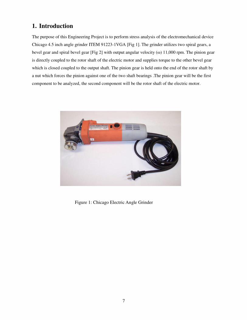
The purpose of this Engineering Project is to perform stress analysis of the electromechanical device

Chicago 4.5 inch angle grinder ITEM 91223-1VGA [Fig 1]. The grinder utilizes two spiral gears, a

bevel gear and spiral bevel gear [Fig 2] with output angular velocity (ω) 11,000 rpm. The pinion gear

is directly coupled to the rotor shaft of the electric motor and supplies torque to the other bevel gear

which is closed coupled to the output shaft. The pinion gear is held onto the end of the rotor shaft by

a nut which forces the pinion against one of the two shaft bearings .The pinion gear will be the first

component to be analyzed, the second component will be the rotor shaft of the electric motor.

Figure 1: Chicago Electric Angle Grinder

8

Figure 2: Spiral bevel gear (large) and a spiral bevel pinion gear (small)

Figure 3 shows the complete component assembly of the grinder. The motor is on the left,

surrounding the rotor shaft. The gearing system is enclosed inside the gear box on the right.

Figure 3: Complete Component Assembly

9

Figure 4 shows the spiral bevel pinion gear attached to the end rotor shaft by a nut.

Figure 4: Shaft with Bevel Pinion Gear

Figure 5 shows the two bearings attached to the end of the shaft (while the pinion gear has been

removed for hardness testing – Fig 6).

Figure 5: Shaft with Bevel Pinion Gear Removed

10

Figure 6: Spiral bevel pinion gear

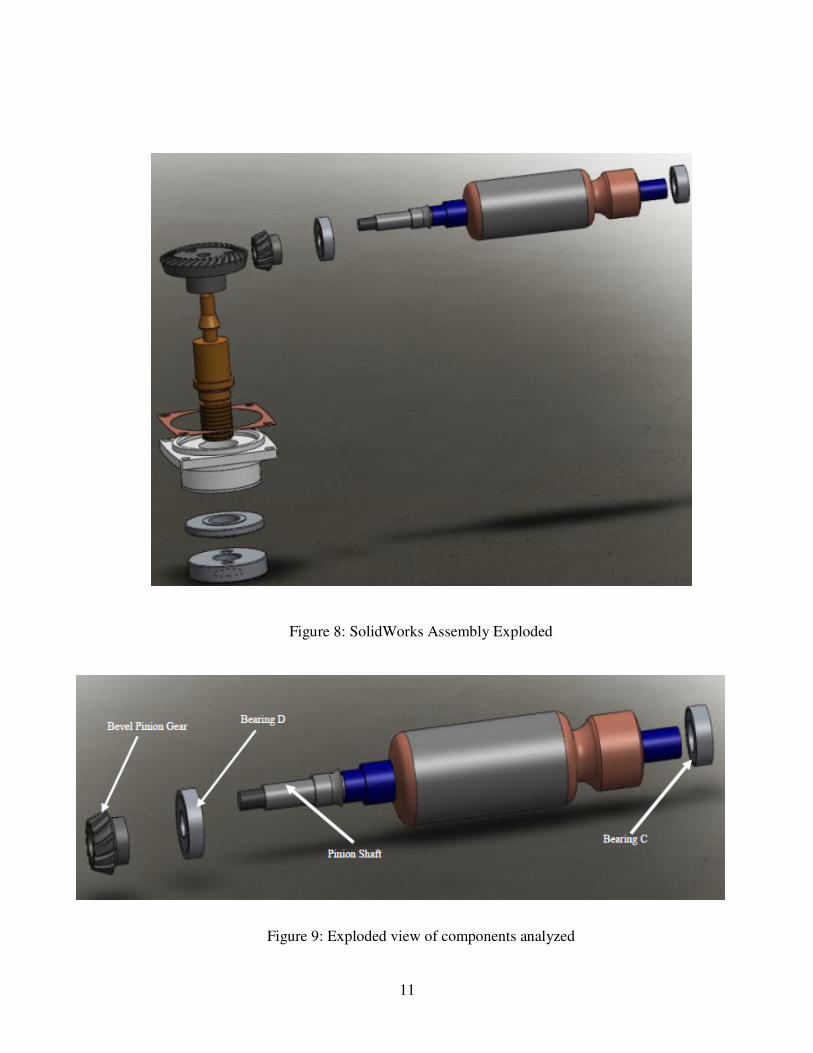
Figure 7 shows the Solid Works representation of the assembly (bevel pinion gear, pinion shaft,

bevel shaft, bearings, bevel gear, bevel casting, chuck washer, washer), Figure 8 shows an

exploded view and Figure 9 shows a detailed view of the two components that will be analyzed ,

the bevel pinion gear and the shaft.

Figure 7: SolidWorks Model Assembly

11

Figure 8: SolidWorks Assembly Exploded

Figure 9: Exploded view of components analyzed

12

2. Data

Table 1 shows the given manufacturing specifications of the machine.

Table 1 Manufacturing Specifications

Angular Velocity 11,000 rev/min

Voltage 110 Volts

Frequency (AC) 60 Hz single phase

Power 570 watts

Amperage 4.5 amps

For single phase armature motors one hp is generated by 720 watts. Assuming that the most

efficiency expected out of a single phase motor is approximately 60% the motor power is calculated as

For proper analysis, additional data must be collected. The material used in the angle grinder was

unknown, therefore it was necessary to perform hardness testing to obtain material data. A

Rockwell Hardness Testing Machine was used to measure the hardness of the shaft and bevel

pinion gear. The bevel gear was completely isolated from its main subassembly. This ensured no

cutting of material or extended surface hardening from clamping and pulling. The shaft was

permanently fixed to its immediate subassembly. Luckily the shaft was just long enough to get

true readings.

Figure 10 shows the hardness test machine use d in this work. Before the hardness test, proper

surface preparation was needed to ensure proper results. Three readings were done on the shaft as

well as on the bevel in different locations to obtain an average hardness number. The location of

testing on the material was also changed to get a variety of readings and to avoid tainted results from

nearby surface hardening created by testing. It is imperative to note that the material will be much

harder on the tooth of the gear rather than in the makeup material. There was no way to test the

hardness of the material directly on the tooth without risking safety for the holder. The reading,

however, was done as close as possible to the side of the tooth without risking the ball sliding

down the face of the tooth. The results are shown in table 2.

hpw

whp

4

3

720

570≈=

13

Figure 10: ME-2 Rockwell Hardness Testing System

Table 2: Hardness Testing Result

Using a hardness conversion chart [2] and the information from Shigley’s Mechanical

Engineering Design in Table 5 [3], material grade and tensile strength can be determined and the

result for the shaft is shown highlighted in table 3.

14

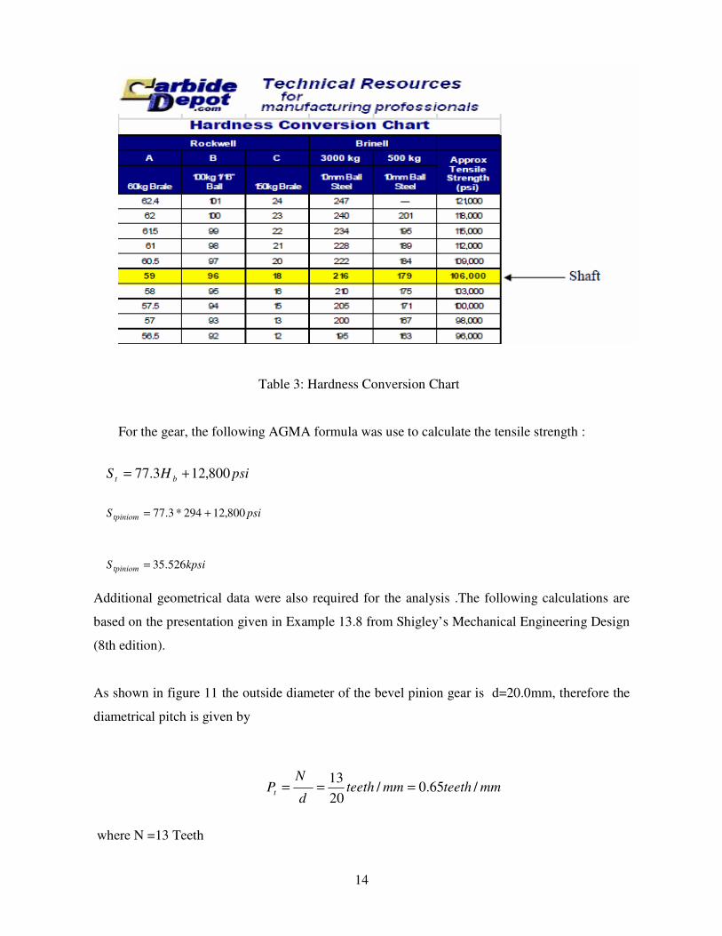
Table 3: Hardness Conversion Chart

For the gear, the following AGMA formula was use to calculate the tensile strength :

Additional geometrical data were also required for the analysis .The following calculations are

based on the presentation given in Example 13.8 from Shigley’s Mechanical Engineering Design

(8th edition).

As shown in figure 11 the outside diameter of the bevel pinion gear is d=20.0mm, therefore the

diametrical pitch is given by

where N =13 Teeth

psiHS bt 800,123.77 +=

kpsiS tpiniom 526.35=

psiS tpiniom 800,12294*3.77 +=

mmteethmmteethd

NPt /65.0/

20

13===

15

The helical angle needed to be determined. In the illustration below, lines were added and

a protractor was used to measure it.

Figure 11: Pinion Close-up with Reference Lines

By using the reference lines the helical angle was measured to be 40 degrees.

The normal diametrical pitch is calculated with the following formula

and the formula below is used to calculate the Pitch diameter

The obtained data are summarized in table 4.

Table 4: Data of the gear and shaft

ϕcos

t

n

PP =

mmteethmmteethP n /8485.0/40cos

65.0==

o

mmmmteeth

teeth

P

Nd

n

p 32.15/8485.0

13===

16

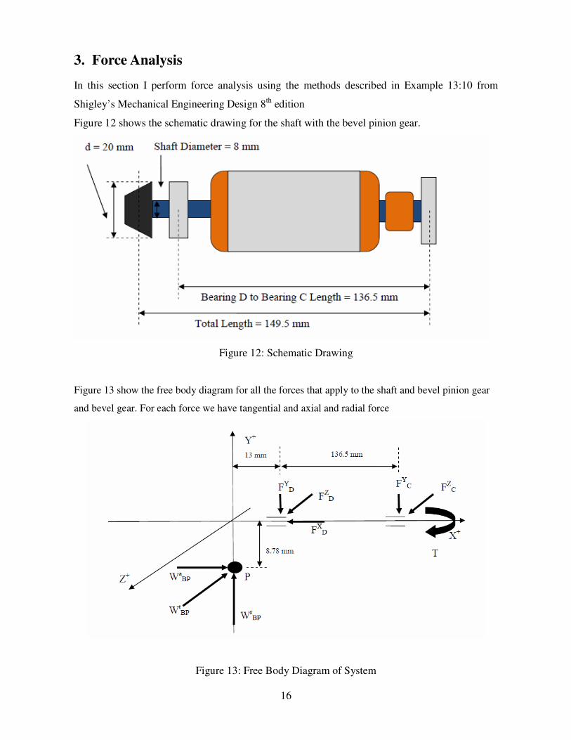
3. Force Analysis

In this section I perform force analysis using the methods described in Example 13:10 from

Shigley’s Mechanical Engineering Design 8th

edition

Figure 12 shows the schematic drawing for the shaft with the bevel pinion gear.

Figure 12: Schematic Drawing

Figure 13 show the free body diagram for all the forces that apply to the shaft and bevel pinion gear

and bevel gear. For each force we have tangential and axial and radial force

Figure 13: Free Body Diagram of System

17

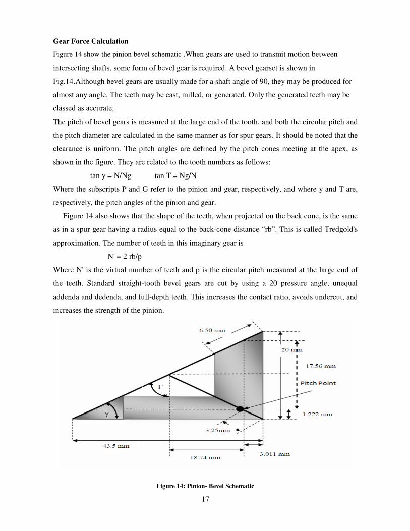
Gear Force Calculation

Figure 14 show the pinion bevel schematic .When gears are used to transmit motion between

intersecting shafts, some form of bevel gear is required. A bevel gearset is shown in

Fig.14.Although bevel gears are usually made for a shaft angle of 90, they may be produced for

almost any angle. The teeth may be cast, milled, or generated. Only the generated teeth may be

classed as accurate.

The pitch of bevel gears is measured at the large end of the tooth, and both the circular pitch and

the pitch diameter are calculated in the same manner as for spur gears. It should be noted that the

clearance is uniform. The pitch angles are defined by the pitch cones meeting at the apex, as

shown in the figure. They are related to the tooth numbers as follows:

tan y = N/Ng tan T = Ng/N

Where the subscripts P and G refer to the pinion and gear, respectively, and where y and T are,

respectively, the pitch angles of the pinion and gear.

Figure 14 also shows that the shape of the teeth, when projected on the back cone, is the same

as in a spur gear having a radius equal to the back-cone distance “rb”. This is called Tredgold's

approximation. The number of teeth in this imaginary gear is

N' = 2 rb/p

Where N' is the virtual number of teeth and p is the circular pitch measured at the large end of

the teeth. Standard straight-tooth bevel gears are cut by using a 20 pressure angle, unequal

addenda and dedenda, and full-depth teeth. This increases the contact ratio, avoids undercut, and

increases the strength of the pinion.

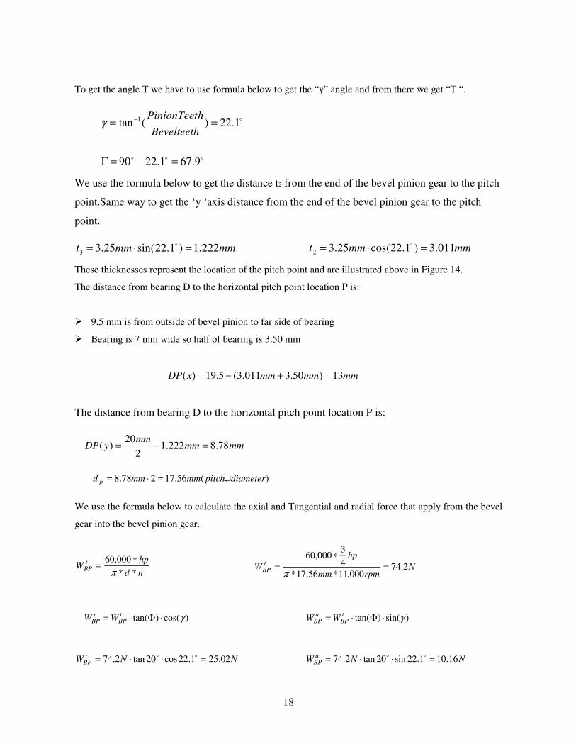
Figure 14: Pinion- Bevel Schematic

18

To get the angle T we have to use formula below to get the “y” angle and from there we get “T “.

We use the formula below to get the distance t2 from the end of the bevel pinion gear to the pitch

point.Same way to get the ‘y ‘axis distance from the end of the bevel pinion gear to the pitch

point.

These thicknesses represent the location of the pitch point and are illustrated above in Figure 14.

The distance from bearing D to the horizontal pitch point location P is:

� 9.5 mm is from outside of bevel pinion to far side of bearing

� Bearing is 7 mm wide so half of bearing is 3.50 mm

The distance from bearing D to the horizontal pitch point location P is:

We use the formula below to calculate the axial and Tangential and radial force that apply from the bevel

gear into the bevel pinion gear.

o1.22)(tan 1 == −

Bevelteeth

hPinionTeetγ

ooo 9.671.2290 =−=Γ

mmmmt 011.3)1.22cos(25.32 =⋅= ommmmt 222.1)1.22sin(25.33 =⋅= o

mmmmmmxDP 13)50.3011.3(5.19)( =+−=

mmmmmm

yDP 78.8222.12

20)( =−=

)(56.17278.8 diameterpitchmmmmd p ↵=⋅=

nd

hpW

tBP

**

000,60

π∗

= Nrpmmm

hp

WtBP 2.74

000,11*56.17*

4

3000,60

=∗

=π

)cos()tan( γ⋅Φ⋅= tBP

rBP WW )sin()tan( γ⋅Φ⋅= t

BPa

BP WW

NNWr

BP 02.251.22cos20tan2.74 =⋅⋅= ooNNW

aBP 16.101.22sin20tan2.74 =⋅⋅= oo

19

Shaft Force Calculations:

Figure 15 shows the free body diagram for the shaft, with all the forces applied by the bearings and

the bevel gear.

Taking the moment around D:

Figure 15: Force Analysais 2-D Planes

(x-y) plane:

So we take the moment at the point D to get the one equation with one unknown, and from there we solve

for the force ycF

The total force in X direction equal to zero (static condition), to calculate the force xDF

{ NkjiW 2.7402.2516.10 −+=v

NWABSW 96.78)( ==

↑=↑⋅−= NdirectionchangeNFy

c 73.1)(73.1

013.02.2578.816.105.136 =−⋅+⋅−=∑ mmNmmNmmFMy

cD

0=−=→∑ XD

ax FWF ←= NF x

D 16.10

20

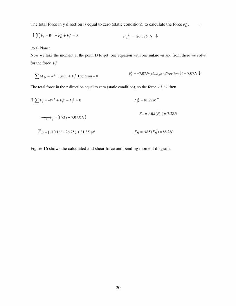
The total force in y direction is equal to zero (static condition), to calculate the force yDF . .

(x-z) Plane:

Now we take the moment at the point D to get one equation with one unknown and from there we solve

for the force zcF

The total force in the z direction equal to zero (static condition), so the force zDF is then

Figure 16 shows the calculated and shear force and bending moment diagram.

0=+−=↑∑ yc

yD

ry FFWF ↓= NF y

D 75.26

05.136.13 =+⋅=∑ mmFmmWMz

ct

D

↓=↓⋅−= NdirectionchangeN 07.7)(07.7Fzc

0=−+−=↑∑ ZC

ZD

tz FFWF ↑= NF

ZD 27.81

)( NKjcF

07.773.1 −=→NFABSF CC 28.7)( ==

NKjiF D }3.8175.2616.10{ +−−= NFABSF DD 2.86)( ==

21

Figure 16 : Load, Shear Force, and Bending Moment Diagrams

22

4. Stress Analysis

Bending Stress and Bending Factor of Safety

We use the formula below to calculate the Dynamic Factor (Kv).

The dynamic factor Kv accounts for internally generated gear tooth loads which are induced by

non-uniform meshing action (transmission error) of gear teeth. A quality number value of 6 is

assumed. The transmission accuracy level number (Qv) could be taken as the quality number Qv = 6.

The American gear manufacturing association has defined a set of quality control numbers which can

be taken as equal to the transmission accuracy level number Qv, to quantify these parameters

(AGMA 390.01). Classes 3< Qv<7 include must commercial quality gears and are generally suitable

for any applications.

We use the formula below to calculate the velocity in secm

Bv

A

VAK )

.200(

+=

32

)12(25.0)1(5650 vQifBBA −=⇒−+=

8254.0)612(*25.0 32

=−=B 77.59)8254.01(5650 =−+=A

60

** pp ndV

π=

59.1)77.59

sec/114.1020077.59( 8254. =

⋅+=

mK v

secsec 114.108.113,1060

min/000,11*56.17*mmm

revmmV ===

π

Bv

A

VAK )

.200(

+=

23

The overload Factor (Ko), assuming uniform loading is Ko = 1.

The Size Factor Ks is calculated using table 14-2 [5] in Shigley’s Mechanical Engineering Design. 8th

Ed. (s, Yp (13T)and value is 0.261 .

The width 6.5 mm →6.5 mm/25.4 mm/in= 0.2559 in hence

P = 0.8485 Teeth/mm = 21.552 Teeth/inch

This is for standard units

Assuming uncrowned so (load correction factor) Cmc=1

In (Pinion Proportion factor) Cpf;

Cpm (pinion proportion modifier) =1.0

Cma(Mesh alignment factor)

Using the table 14.9 [6], Value for A, B, C are as follows:

A=0.127

B=0.0158

0535.0)(192.11

P

YF

kK

bs ∗==

907.0)/552.21

261.0*2559.0(*192.1)(192.1

1 0535.00535.0 ==∗==inT

in

P

YF

kK

b

s

)(*1 ** emapmpfmcmfH CCCCCCK ++==

00.10≤F

0120.0025.056.17*10

5.6025.0

*10=−=−=

mm

mm

d

FC pf

2CFBFACma ++=

24

Ce(Mesh alignment correction factor )1

The rim thickness factor Kb=1 due to consistent thickness of gear.

Speed Ration mG;

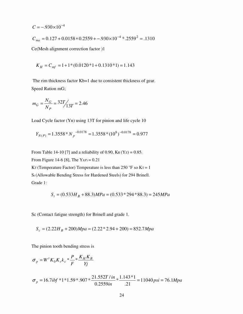
Load Cycle factor (Yn) using 13T for pinion and life cycle 10

From Table 14-10 [7] and a reliability of 0.90, KR (YZ) = 0.85;

From Figure 14-6 [8], The YJ(P) = 0.21

KT (Temperature Factor) Temperature is less than 250 °F so KT = 1

St (Allowable Bending Stress for Hardened Steels) for 294 Brinell.

Grade 1:

Sc (Contact fatigue strength) for Brinell and grade 1.

The pinion tooth bending stress is

410930. −×−=C

1310.2559.*10930.2559.00158.0127.024 =×−+∗+= −

maC

143.1)1*1310.01*0120.0(*11 =++== mfH CK

46.213

32 ===T

TN

Nm

P

GG

977.0)10(*3558.1*3558.1 0178.080178.0)( === −−

pPN NY

MPaMPaHS Bt 245)3.88*294*533.0()3.88533.0( ==+=

MpaMpaHS Bc 7.852)20094.2*22.2()20022.2( =+=+=

Mpapsiin

inTibfp 1.7611040

21.

1*143.1*

2559.0

/552.21*907.*59.1*1*7.16 ===σ

Yj

KK

F

PkKKW BH

svt

p **0=σ

25

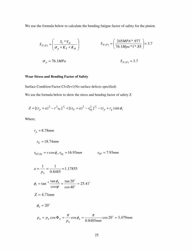
We use the formula below to calculate the bending fatigue factor of safety for the pinion

Wear Stress and Bending Factor of Safety

Surface Condition Factor Cf=Zr=1(No surface defects specified)

We use the formula below to show the stress and bending factor of safety Z

Where;

∗∗=

RTp

NtPF

KK

YSS

σ*

)(7.3

85.*1*1.76

977.*245)( =

=

Mpa

MPAS PF

MPap 1.76=σ 7.3)( =PFS

tgpbgGbpp rrrarrarZ φsin)(])[(])[( 21

21 2222 +−−++−+=

mmrp 78.8=

mmrG 74.18=

mmrbP 93.7=mmrrr bgtbpbG 93.16,cos, == φ

17855.18485.0

11===

npa

mmZ 71.4=

o

o

o

41.2540cos

20tan

cos

tantan 1 === −

ψφ

φ nt

o20=nφ

mmmmp

pp n

n

nnn 479.320cos8485.0

coscos ===Φ= oπφ

π

26

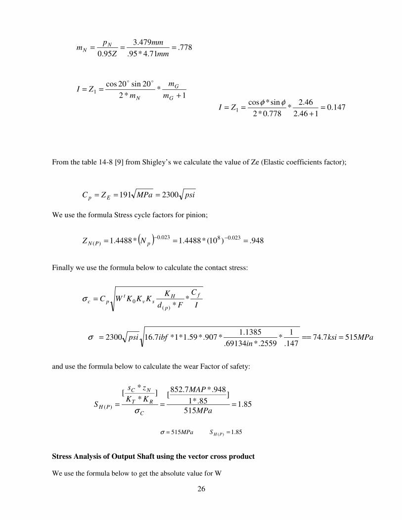
From the table 14-8 [9] from Shigley’s we calculate the value of Ze (Elastic coefficients factor);

We use the formula Stress cycle factors for pinion;

Finally we use the formula below to calculate the contact stress:

and use the formula below to calculate the wear Factor of safety:

MPa515=σ 85.1)( =PHS

Stress Analysis of Output Shaft using the vector cross product

We use the formula below to get the absolute value for W

778.71.4*95.

479.3

95.0===

mm

mm

Z

pm N

N

147.0146.2

46.2*

778.0*2

sin*cos1 =

+==

φφZI

1*

*2

20sin20cos1 +

==G

G

N m

m

mZI

oo

psiMPaZC Ep 2300191 ===

( ) 948.)10(*4488.1*4488.1 023.08023.0)( === −−

pPN NZ

I

C

Fd

KKKKWC

f

p

Hsv

tpc *

*)(0=σ

MPaksiin

ibfpsi 5157.74147.

1*

2559.*69134.

1385.1*907.*59.1*1*7.162300 ====σ

85.1515

]85.*1

948.*7.852[]

*

*[

)( ===MPa

MAP

KK

zs

SC

RT

NC

PH σ

27

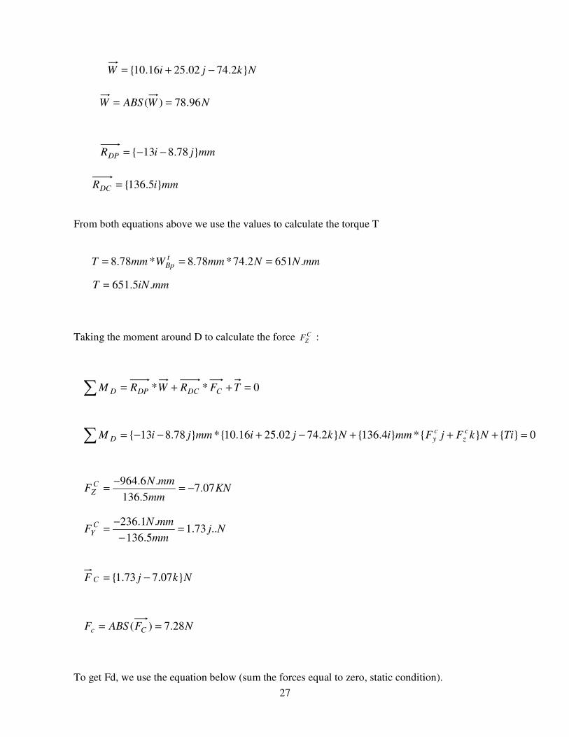
From both equations above we use the values to calculate the torque T

Taking the moment around D to calculate the force CZF :

To get Fd, we use the equation below (sum the forces equal to zero, static condition).

NkjiW }2.7402.2516.10{ −+=

NWABSW 96.78)( ==

mmjiRDP }78.813{ −−=

mmiRDC }5.136{=

mmNNmmWmmTt

Bp .6512.74*78.8*78.8 ===

mmiNT .5.651=

0** =++=∑ TFRWRM CDCDPD

0}{}{*}4.136{}2.7402.2516.10{*}78.813{ =+++−+−−=∑ TiNkFjFmmiNkjimmjiMcz

cyD

KNmm

mmNF

CZ 07.7

5.136

.6.964−=

−=

Njmm

mmNF

CY ..73.1

5.136

.1.236=

−−

=

NkjF C }07.773.1{ −=

NFABSF Cc 28.7)( ==

28

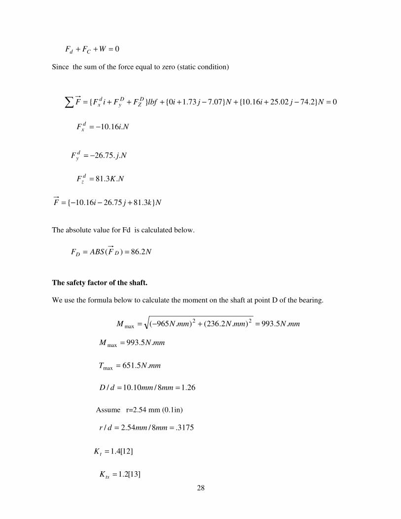
Since the sum of the force equal to zero (static condition)

The absolute value for Fd is calculated below.

The safety factor of the shaft.

We use the formula below to calculate the moment on the shaft at point D of the bearing.

Assume r=2.54 mm (0.1in)

0=++ WFF Cd

0}2.7402.2516.10{}07.773.10{}{ =−++−++++=∑ NjiNjilbfFFiFFD

ZDy

dx

NiFd

x .16.10−=

NjFdy ..75.26−=

NKFd

z .3.81=

NkjiF }3.8175.2616.10{ +−−=

NFABSF DD 2.86)( ==

mmNmmNmmNM .5.993).2.236().965( 22max =+−=

mmNM .5.993max =

mmNT .5.651max =

26.18/10.10/ == mmmmdD

3175.8/54.2/ == mmmmdr

]12[4.1=tK

]13[2.1=tsK

29

Notch sensitivity (q) =0.95[14]

Shear notch sensitivity (qshear)=1 [15]

Assume Sy=0.775Sut

Sut=106Ksi = 730.8MPa

So the safety factor of the shaft is calculated using the formula below.

Fatigue Factor of Safety Calculations

Analysis based on Modified Goodman Design Theory

Using the table 6-2[5] from Shigley’s and assuming a surface finishes of mechanized or cold

drawn:

a=4.51

b=-0.265

38.1)14.1(95.01)1(1 =−+=−+= tf KqK 2.1)12.1(11)1(1 =−+=−+= tssfs KqK

MPamm

mmN

d

MK fa 28.27

)8.(

.5.993*3238.1

.

.3233

max" ===ππ

σ

2

3

max"]

.

.16.[3

d

TK fsm

πσ =

MPamm

mmNm 47.13]

)8.(

.5.651*.162.1.[3

2

3

" ==π

σ

''am

y

yield

Sn

σσ +=

9.1328.2747.13

8.730*775.0=

+=

MPaMPa

MPan yield

ute SS *5.0' =

MPaMPaSe 4.3658.730*5.0' ==

30

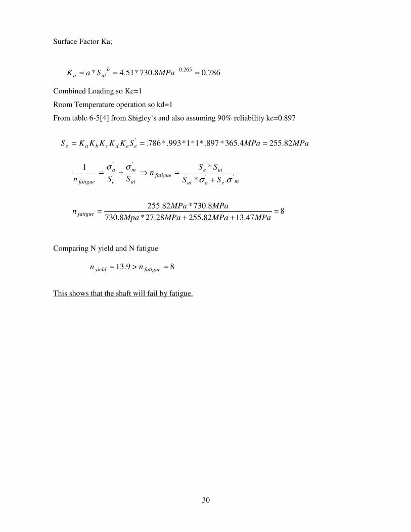
Surface Factor Ka;

Combined Loading so Kc=1

Room Temperature operation so kd=1

From table 6-5[4] from Shigley’s and also assuming 90% reliability ke=0.897

Comparing N yield and N fatigue

This shows that the shaft will fail by fatigue.

786.08.730*51.4*265.0 === −

MPaSaKb

uta

MPaMPaSKKKKKS eedcbae 82.2554.365*897.*1*1*993.*786.' ===

meaut

utefatigue

ut

m

e

a

fatigue SS

SSn

SSn ''

''

.*

*1

σσ

σσ

+=⇒+=

847.1382.25528.27*8.730

8.730*82.255=

++=

MPaMPaMPaMpa

MPaMPan fatigue

89.13 =>= fatigueyield nn

31

5. Finite Element Analysis

Figures 17 and 18 show the load and restraint setup on Cosmos software. The green arrows in

the pictures represented the mechanical constrain impose by bearings D and C on the shaft.

At bearing D, radial and axial restraints were set. Restraints were applied to a 2 mm cylindrical face

placed at the midpoint of the bearing location. The bearing restraint at C was set for only a rotational

restraint. This was to ensure that over-constraining the shaft was avoided. This restraint was also

applied to a 2 mm cylindrical face placed at the midpoint of the bearing location.

Figure 17: Restraints at Bearing D

Figure 23: Restraints at Bearing C

Figure 18: Loads at Pitch Point Applied Using Remote Load

32

'maxσ

Figure 19 shows the shaft with constraints and loads and the computed values of the von Mises stress

are also shown. The maximum stress (=28.12 MPa ) appears on the bearing area.An expanded view

of the most highly stressed area is shown in figure 20.

Figure 19: Shaft with Constraints and Loads and Study Run

Figure 20: Probe Value of Maximum Stress

33

'maxσ

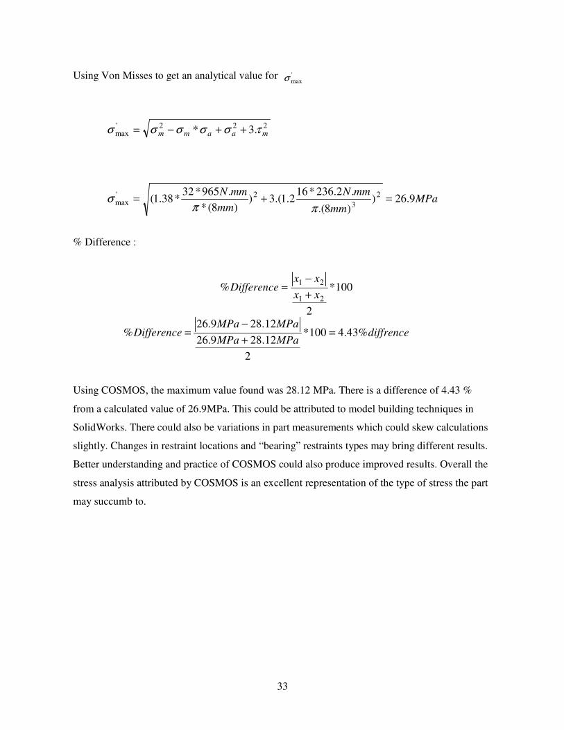
Using Von Misses to get an analytical value for

% Difference :

Using COSMOS, the maximum value found was 28.12 MPa. There is a difference of 4.43 %

from a calculated value of 26.9MPa. This could be attributed to model building techniques in

SolidWorks. There could also be variations in part measurements which could skew calculations

slightly. Changes in restraint locations and “bearing” restraints types may bring different results.

Better understanding and practice of COSMOS could also produce improved results. Overall the

stress analysis attributed by COSMOS is an excellent representation of the type of stress the part

may succumb to.

222'max .3* maamm τσσσσσ ++−=

MPamm

mmN

mm

mmN9.26)

)8.(

.2.236*162.1.(3)

)8(*

.965*32*38.1( 2

3

2'max =+=

ππσ

100*

2

%21

21

xx

xxDifference

+

−=

diffrenceMPaMPa

MPaMPaDifference %43.4100*

2

12.289.26

12.289.26% =

+

−=

34

6. Conclusion

The project exemplified real world tasks that definitely sharpened my skills a young engineer.

The hands-on experience gained by using the laboratory equipment and software tools was

invaluable. The experience of using specific tools, acquiring data, and using this data in

calculations was a particularly useful experience. It provided some relevance of the knowledge

learned from work experience and my other engineering courses.

Also COSMOS in particular was beneficial not only because I was able to use it as a comparison

tool but also because of the practical experience gained which will be useful in the a ‘real-world’

application. This tool gives a visual representation of the types of stresses and possible

deformations that may occur in design. This quick reference will give the design engineer an

approximation of what to expect under certain loads or applications. This brief exposure to

COSMOS will certainly be invaluable.

Reference

[1] Manufacturing Specifications link,

http://www.harborfreight.com/cpi/ctaf/displayitem.taf?Itemnumber=43471

p/english/gear/myset/spiral.html

[2] Hardness conversion chart,

http://www.carbidedepot.com/formulas-hardness.htm

[3] AGMA Strength Graph for Hardened Steels,

Budynas, R., Nisbett, K., Shigley’s Mechanical Engineering Design. 8th Ed. McGraw Hill, New

York NY, 2008. pp 727

[4] Reliability Assumption,


York NY, 2008. Table 6-5, pp 285

[5] Parameters for Marin Surface Modification Factors,


York NY, 2008. Table 6-2, pp 280

[6] Lewis Form Factor,


York NY, 2008. Table 14-2, pp 718

35

[7] Empirical Constants for Load Distribution Factor


York NY, 2008. Table 14-9, pp 740

[8] Reliability Factor KR


York NY, 2008. Table 14-10, pp 744

[9] Geometry Factor,


York NY, 2008. Figure 14-6, pp 727

[10] For Elastic Coefficient,


York NY, 2008. Table 14-8, pp 737

[12] For Stress Concentration Value Kt,


York NY, 2008. Appendix Figure 15-6, pp 1007

[13] For Stress Concentration Value Kts.


York NY, 2008. Appendix Figure 15-8, pp 1008 32

[14] Notch Sensitivity q,



[15] Shear Notch Sensitivity q,



[16] pitch diameter p,


York NY, 2008. Example 13:15, pp 245

Zouhri-Final Report

Documents

Transcript of Zouhri-Final Report