Final report

Intercomparison on water-/heatmeters at 50 °C and 1-20 m³/h

EUROMET Project No. 863

VMH Heikkilä Oy

Peter Lau and Krister Stolt Borås 2007

2

Abstract A Nordic flow meter inter-comparison on water/heatmeters at a temperature of 50 °C was performed involving 10 laboratories from eight countries. The participants were National Laboratories or were recommended to participate by a National Laboratory. SP as the pilot laboratory selected four flow meters and assembled these in a compact package that was transported by the project leader as an assembled unit between the laboratories. Each participant had only two days for the calibration, simulating an everyday work task. Thus all experimental work could be done within a four month period. The two reference val-ues for mass and volume were defined by combining the two mass flow meters and se-lecting the most suitable magnetic inductive meter respectively. The total agreement be-tween the participants with respect to the two references at all five flow rates was better than ± 0,2 % at a 95 % confidence level. Key words: Inter-comparison, heat meters, transfer standards, class 1 meter SP Sveriges Tekniska SP Technical Research Institute of Forskningsinstitut Sweden

SP Rapport: 2007:01 SP Report: 2007:01

ISBN 91-85533-64-5 ISSN 0284-5172 Borås Postal address: Box 857, SE-501 15 BORÅS, Sweden Telephone: +46 10 516 50 00 Telefax: +46 33 10 69 73 E-mail: info@sp.se www.sp.se

3

Contents

Abstract 2

Contents 3 Foreword 4 Sammanfattning 5 1 Presentation of the inter-comparison 7

1.1 The scope 7 1.1.1 The participating laboratories 7 1.1.2 The transfer standards 7 1.1.3 Preconditions and way of performing the calibration 8 1.1.4 The time schedule 9 2 Detailed information on the used calibration objects 10

2.1 Test scheme of the inter-comparison 10 2.2 Meter behaviour before and after the inter-comparison 10 2.2.1 Meter characterization 11 2.2.2 Repeatability and reproducibility 11 2.2.3 Temperature dependency and need of correction 11 2.2.4 Pressure dependency and need for correction 11 3 Inter-comparison results and analysis 12

3.1 Choice of reference 12 3.2 Inter- and intra repeatability/reproducibility in comparison 12 3.2.1 Repeatability 12 3.2.2 Reproducibility 13 3.3 Youden plot 14 3.4 Calibration results for the different meters 15 3.4.1 Mass flow meters CMF200 and CMF050 15 3.4.2 Volume flow meters Enermet and K40 20 3.5 Uncertainty claims 21 3.6 Consistency test of the results 21 3.7 Construction of the reference points 22 3.8 En-value test 23 4 Interpretation of results and conclusions 24

5 References 25

Appendix

1 Protocol form i 2 Primary measurement data i 3 Calculation of repeatability /reproducibility ii 4 Temperature behaviour of the important meters iii 5 Pressure dependency vii 6 Detailed Youden plots viii 7 Consistency test results ix

4

Foreword Energy distribution via hot water in district heating is an important aspect in the Nordic countries. The accuracy in energy measurement depends predominantly on the volume measurement of the hot water. The wish to introduce a class 1 heat meter on a European level, meaning a permitted error of indication of not more than 1 %, could so far not be realized. Although many laboratories have claimed calibration uncertainties in the range of 0,1 %, no good enough international agreement could be found, that verifies this claim. What was needed was an inter-comparison to show that the uncertainties of the laborato-ries are not greater than one fifth of 1 % (±0,2 %) to support the introduction of this class of heat meters. There are several reasons why this goal previously has not been reached. Most important is probably the meter stability and the reproducibility conditions when mounting and dismounting, thus meaning that the laboratories ability of meter calibration has been overlaid by other effects. The new approach of this inter-comparison was to keep all conditions concerning the meters behaviour between the laboratories as identical as possible and also to generate work conditions that are as close as possible to a routine measurement. For this reason, up to four meters were circulated as one compact and never changed or dismounted package and not more than two days were allowed for the measurements at each laboratory. This inter-comparison was performed by ten laboratories from eight Nordic and Baltic countries. The outcome is very encouraging showing that even laboratories that never before have taken part in an inter-comparison, do have the capability for an accurate hot water meter/flow sensor calibration, and this despite their claims that in some cases are much more modest. This thus makes it possible for these laboratories to support the in-spection bodies for heat meters in their respective country. Thanks to this project, which thankfully was sponsored by NICe (The Nordic Innovation Centre), it could be shown that there is a general agreement between the Nordic and Bal-tic countries to make the class 1 heat meters, according to the MID directive 2004/22/EC and the standard EN1434, a reality in Europe.

5

Sammanfattning Föreliggande rapport beskriver en jämförelsemätning med vattenmätare/värmemätare gjort med vatten vid 50 °C mellan tio laboratorier i åtta nordiska länder. SP som pilotla-boratoriet valde ut fyra mätare i serie, två massflödesmätare av coriolis typ och två mag-netisk induktiva mätare vilka var hopbyggda till en kompakt enhet som inte ändrades eller demonterades någon gång under hela tiden. Varje deltagande laboratorium fick två dagar för sin kalibrering, vilket ansågs motsvara normala rutinförhållanden och projekt ledaren tog ansvar för hela transporten, vilket innebar den korta perioden av fyra månader att slutföra alla mätningar. Referensvärdet för massan/volymen bestämdes genom parvis kombination av respektive mätartyper. Den sammanlagda överensstämmelsen mellan deltagarna med hänsyn till referensvärden och alla fem flöden låg med 95 % sannolikhet inom en marginal på ±0,2 %, vilket är tillåten mätosäkerhet vid provning av klass 1 flö-desgivare i värmemätare i mätinstrumentdirektivet 2004/22/EC och standarden EN1434.

6

7

1 Presentation of the inter-comparison Flow or volume measurement with the help of flow meters concerns a dynamic quantity. The reference equipment used in calibration, the flow rigs, are mostly tailor built and a correct calibration result is to a high extend dependent on the applied method and the skill and experience of the staff. Despite the dynamic measurement process the traceability is almost always to a statically determined mass of liquid. The only generally accepted and known way to secure the calibration quality, is by exchanging stable transfer standards and to compare the outcome with other laboratories.

1.1 The scope This inter-comparison concerned hot water meters/flow sensors in heat meters and had two objectives. The first one was to help the involved laboratories in the qualification of their calibration service. For several of them this was their first experience of an interna-tional comparison. The second objective was to investigate if the inter-laboratory agree-ment would be good enough to support the introduction of a class 1 for heat meters as suggested by the MID-directive [1]. A class 1 meter has a maximum permissible error (MPE) of ±1 %. The requested uncertainty in calibration or test of such a meter therefore should be 1/5, i.e. ±0,2 %. The wish for such an agreement had existed for many years, but could not be realized. [2] 1.1.1 The participating laboratories The following 10 laboratories from 8 countries took part in this inter-comparison. They are listed in the order of performing the calibration measurement. Table 1

Laboratory: Country: Name of institution: Lab no: Iceland Frumherji 1 DTI Denmark Danish Teknologisk Institute 2 Force Denmark Force Technology 3 JV Norway Justervesenet 4 VMH Finland VMH Heikkilä Oy 5 Metrosert Estonia Ltd Metrosert 6 Tepso Estonia Ltd Tepso 7 LNMC Latvia Latvian National Metrology Centre 8 LEI Lithuania Lithuanian Energy Institute 9 SP* Sweden Technical Research Institute of Sweden 10 * Pilot Laboratory

1.1.2 The transfer standards Traditionally flow transfer meter packages have consisted of two identical meters. There are however good arguments for using two different kinds of meters, based on different measurement principles, which lately has been the rule. In this exercise altogether 4 me-ters in series were calibrated simultaneously (only one laboratory calibrated the meters separately but still in an assembled package). One of the meters had previously been used as reference meters in various comparisons and had been well proved to be suitably sta-ble. The meters are arranged in a rig construction and transported as one unit on a small trolley, see figure 1a to 1c where also the reference meters can be seen. The meters are

8

further presented in chapter 2. In the round robin a pipe through the filter provides a straight inlet to the K40 of 32 cm or 7 to 8 D length.

Fig 1a. Trolley exposing the small coriolis meter

Fig 1b. Meters in series and signal panel

Fig 1c. Flow path through the package Fig 1d. Connection to the reference test rig The meters on the trolley are connected to the test rigs in the respective laboratory via hoses as shown in figure 1d. This package construction was expected to produce equal conditions concerning installa-tion related effects and thus improve the reproducibility of all meters.

1.1.3 Preconditions and way of performing the calibration Traditionally in inter-comparisons, transfer flow meters are packed in boxes and shipped between the laboratories, where they were unpacked and installed into the test section of the calibration facility. The pack boxes contain more or less detailed installation advices and a well worked out test procedure. Laboratories usually have two to four weeks to become acquainted to the meters and to perform the calibrations. It happens occasionally, as also in this inter-comparison, that a laboratory is faced with a meter type it has not calibrated before, which might have some impact on the result. This Nordic inter-comparison differs in some important aspects from the standard proce-dure:

9

• The package was assembled all the time • The time for calibration was limited to two working days • The project leader from the pilot laboratory followed the package during trans-

portation and calibration. This means that the meters were ready for calibration directly after connection to the flow rig. Possible installation related effects on the meters should be identical during the whole exercise. The traceability in each laboratory and the measurement and calibration skills were the main interest in this inter-comparison. Two working days were expected to be enough to start and complete the job, which is a realistic approach simulating a standard situation in calibration of customer’s objects. The third point above is important to mention. The visit was announced and the transpor-tation accomplished by the project leader by car. A fundamental idea was to keep a tight time schedule. The meters were never exposed to any risk of damage during transporta-tion and handling or other unexpected disturbances or changes during the whole round robin. Such risks could otherwise be, e.g. unwanted zeroing of the coriolis meters, varia-tions in thermal insulation during the measurement or different preparation before trans-portation. The decision of having the project leader being present at any stage of the comparison is based on earlier experience, where unnecessary effort was put into investigations of sig-nificant differences between the laboratory results. Also practical issues, such as ATA-carnet related problems concerning Island and Norway, could be solved at once without causing common delays in such exercises. A self-evident purpose with the round robin is to test the laboratories capability to per-form calibrations under routine like conditions. This includes of course the skill of the staff. On the other hand one also should mention that there is a risk that practical precau-tions that might be overlooked in a routine type calibration performed with unknown meters might be blocked by a too helpful project leader. But some help with conditioning meter signals in order to speed up the measurement process does certainly not disqualify a laboratory. Actually the K40 magnetic inductive meter showed some peculiar signal irregularities at the end of the round robin that, due to the project leader’s experience, could be directed to the meters electronic behaviour and this did not cause a delay in the measurement and evaluation. The project leader thus could make the measurements more efficient without assisting in aspects which are essential for the performance of the laboratory. A further aspect that needs to be mentioned is the insulation of the meters that was done in the same way by the project leader using blankets. At least at low flow rates this is otherwise an important source for spread between laboratories.

1.1.4 The time schedule The whole round robin started in September 2005 with a first measurement at SP. The package then followed the order of the laboratories listed in table 1. The concluding measurement was performed in December of the same year, i.e. within four months. Flow inter-comparisons with ten laboratories usually tend to take much more than one year. Immediately after the second calibration at SP in mid December all participants met at SP to look at the preliminary results and to discuss the outcome and the evaluation.

10

2 Detailed information on the used calibra-

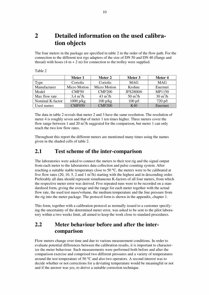
tion objects The four meters in the package are specified in table 2 in the order of the flow path. For the connection to the different test rigs adapters of the size of DN 50 and DN 40 (flange and thread) with hoses (4 m + 2 m) for connection to the trolley were supplied. Table 2

Meter 1 Meter 2 Meter 3 Meter 4

Type Coriolis Coriolis MAG MAG Manufacturer Micro Motion Micro Motion Krohne Enermet Model CMF50 CMF200 JFS2800/6 MP1150 Max flow rate 3,4 m3/h 43 m3/h 50 m3/h 30 m3/h Nominal K-factor 1000 p/kg 100 p/kg 100 p/l 720 p/l Used names CMF050 CMF200 K40 Enermet The data in table 2 reveals that meter 2 and 3 have the same resolution. The resolution of meter 4 is roughly seven and that of meter 1 ten times higher. Three meters cover the flow range between 1 and 20 m3/h suggested for the comparison, but meter 1 can only reach the two low flow rates. Throughout this report the different meters are mentioned many times using the names given in the shaded cells of table 2.

2.1 Test scheme of the inter-comparison The laboratories were asked to connect the meters to their test rig and the signal output from each meter to the laboratories data collection and pulse counting system. After reaching a suitable stable temperature close to 50 °C, the meters were to be calibrated at five flow rates (20, 10, 5, 2 and 1 m3/h) starting with the highest and in descending order. Preferably all data should represent simultaneous K-factors of all four meters, from which the respective meter error was derived. Five repeated runs were to be recorded on a stan-dardised form, giving the average and the range for each meter together with the actual flow rate, the used test mass/volume, the medium temperature and the line pressure from the rig into the meter package. The protocol form is shown in the appendix, chapter 1. This form, together with a calibration protocol as normally issued to a customer specify-ing the uncertainty of the determined meter error, was asked to be sent to the pilot labora-tory within a two weeks limit, all aimed to keep the work close to standard procedures.

2.2 Meter behaviour before and after the inter-

comparison Flow meters change over time and due to various measurement conditions. In order to evaluate potential differences between the calibration results, it is important to character-ize the meter behaviour. Such measurements were performed both before and after the comparison exercise and comprised two different pressures and a variety of temperatures around the test temperature of 50 °C and also two operators. A second interest was to decide whether or not corrections for a deviating temperature would be meaningful or not and if the answer was yes, to derive a suitable correction technique.

11

2.2.1 Meter characterization The meters are simply characterized in the same way as in the common calibration proce-dure, by determining the respective meter error at five flow rates (qi =20, 10, 5, 2 and 1 [m3/h]).

( ) ( )nomKqKerrormeter mim)absolute( −= (1a)

Here Km(nom) stands for the nominal K-factor appointed to the meter by the supplier telling how many electrical pulses the meter produces for every litre or kilogram of liquid passing the meter. The index m identifies one of the four meters and the argument qi re-minds that the K-factor - and thus the error - can change with flow rate. A more practical definition concerns the relative error which is used in the inter-comparison and given by equation (1b).

( )( ) ( )

( )[ ]%

nomK

nomKqKerrormeterqiE

m

mim)relative(m 100×

−== (1b)

The advantage with this measure is not only that it indicates the meter deviation in per-cent, but also allows to directly judge the difference between different runs, measurement conditions, operators and laboratories.

2.2.2 Repeatability and Reproducibility The repeatability r and reproducibility R figures characterizing the variability in the re-sults, can tell if the meters are suitably stable for a flow meter inter-comparison. There-fore these figures were studied for the intra-laboratory case as well as for the inter-laboratory comparison (se 3.2 and appendix chapter 3). The repeatability was calculated for each measurement series (flow rate and laboratory) and then an average was built.

2.2.3 Temperature dependency and need for correction Flow meters are sensitive for changes in medium temperature. The laws governing the temperature behaviour depend on the physical principals used in the meter. Modern flow meters sometimes have built in temperature correction.

As not all calibrations were performed at the stipulated test temperature of 50 °C, the pilot laboratory studied the possible size of the temperature effect to decide whether or not temperature compensation was necessary. The results of several repeated measure-ments at different temperatures in the range from 40 to 55 °C are reported in the appendix chapter 4. Considering the low temperature sensitivity in connection with temperature deviations of not more than 3 °C, a possible correction is not significant.

2.2.4 Pressure dependency and need for correction Chapter 5 in the appendix also contains a short test showing a minor effect of varying the medium pressure at two flow rates. Also in this case the result indicates no need to look at the pressure data in any detail.

12

3 Inter-comparison results and analysis All laboratories followed the test scheme and reported the results. SP as the pilot labora-tory had two results; one at the beginning and one at the end. To have the same weight as any other laboratory only one result is reported here, which was the last measurement, mainly due to the better temperature control. One laboratory, Iceland, was not able to reach the highest flow rate and thus reported only on four flow rates. Force (Denmark) did not deliver measurement data for the Enermet-meter for the two highest flow rates. JV (Norway) could only sample three meters simul-taneously and selected K40 in the first place, which means that data for Enermet are lack-ing. However the Enermet data showed to be the more reliable, partly due to problems with the K40 electronics in the later part of the comparison. LNMC (Latvia) finally was limited to calibrate only one meter a time, which means that the data from the four meters not necessarily is completely comparable. The following results have to be understood with these limitations.

3.1 Choice of reference meters Although four meters were available, only two were used as a basis for the reference, one referring to mass and one to volume. In the appendix, where some detailed results are shown, it is argued to use a combination of the Micro motion meters CMF050 and CMF200 to build one stable reference for the mass signal. This means the readings of the small flow meter represents the mass signal for flow rate 1 and 2 (qi = 1 and 2 m3/h), whereas the larger one represents the mass signal for flow rate 3, 4 and 5 (qi = 5, 10 and 20 m3/h) and both are treated as if they constituted one single meter. In the comparison of the two Mag-meters, Enermet showed a distinctly better repeatabil-ity and reproducibility than the K40. A consistency test (Chapter 7 in the appendix) also pointed out the Enermet as the best reference for a comparison. A reason for this is probably some signal problems with the K40 in the second half of the round robin.

3.2 Inter- and intra repeatability/reproducibility in

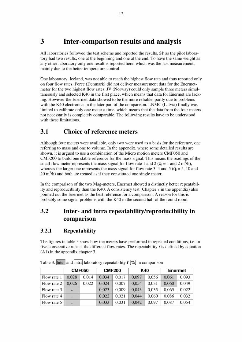
comparison 3.2.1 Repeatability The figures in table 3 show how the meters have performed in repeated conditions, i.e. in five consecutive runs at the different flow rates. The repeatability r is defined by equation (A1) in the appendix chapter 3. Table 3. Inter and intra laboratory repeatability r [%] in comparison

CMF050 CMF200 K40 Enermet

Flow rate 1 0,028 0,014 0,034 0,017 0,097 0,056 0,061 0,093 Flow rate 2 0,026 0,022 0,024 0,007 0,054 0,031 0,060 0,049 Flow rate 3 - 0,023 0,009 0,043 0,035 0,065 0,022 Flow rate 4 - 0,022 0,021 0,044 0,060 0,086 0,032 Flow rate 5 - 0,033 0,031 0,042 0,097 0,087 0,054

13

The shaded columns refer to the average repeatability from all ten laboratories under comparable conditions (~50°C). The figures to the right refer to the average repeatability of the pilot laboratory for comparison. The repeatability characterizes the short term variability in the error determination. Gen-erally the repeatability is flow rate dependent and differs between the meters. It varies typically between 0,022 and 0,097 %. The figures of the pilot laboratory (average over eight measurements) are mostly but not always better than the average of ten laboratories. The factor rintra/rinter is 0,3 to 2,5.

3.2.2 Reproducibility The reproducibility information covers two aspects. It measures the spread between labo-ratories, more exactly the spread between the average meter errors at each flow rate. But it also combines this with the average spread in repeated tests. Thus the reproducibility characterizes meters behaviour in short and long term. However, in an inter-comparison like this, the reproducibility gives a measure for how well the meters can be calibrated in a Nordic perspective including several laboratories with somewhat different measuring conditions. And finally the reproducibility figure can be used to judge the capability of the laboratories to produce this kind of meter calibrations. The reproducibility R is de-fined by equation (A3) in the appendix chapter 3. Table 4 Inter-laboratory reproducibility R in comparison with intra-laboratory data Table 4 Inter-laboratory reproducibility R [%] in comparison with intra-laboratory data

CMF050 CMF200 K40 Enermet

Flow rate 1 0,142 0,075 0,232 0,030 0,522 0,086 0,173 0,157

Flow rate 2 0,122 0,070 0,191 0,016 0,256 0,087 0,184 0,122

Flow rate 3 - - 0,115 0,040 0,182 0,118 0,215 0,099

Flow rate 4 - - 0,106 0,140 0,190 0,233 0,222 0,116

Flow rate 5 - - 0,136 0,284 0,227 0,291 0,187 0,109

Again the inter-laboratory reproducibility in the shaded columns is larger than the corre-sponding data within the pilot laboratory, which is very natural and expected. However the difference is not large. Only in the low flow range of CMF200 and K40 there is a considerable difference, but these data are not used for the detailed comparison. For the rest the factor Rintra/Rinter is 0,35 to 2 indicating a very satisfactory relation, considering ten different rigs and experimenters. The values for K40 in italic style are calculated ex-cluding one measurement series declared as an outlying result. As the error is given in percent, the variability is also in percent. Expressed in words one can state that the error for CMF200 at flow rate 5, found under reproducibility conditions, at average lies within 0,03 ±0,136 % (compare table 6). The intra laboratory reproducibility is based on altogether 8 measurements at tempera-tures between 40 and 55 °C using different pressure and reference volumes and two op-erators and covers a period of roughly five month. But the equipment was the same all the time. If one would have removed some inconsistent results found in a chi-squared test, the two data sets compared would not differ more than a factor two in reproducibility, despite the different equipment and operators. This must be considered as an excellent agreement due to the meter stability and the construction of the package.

14

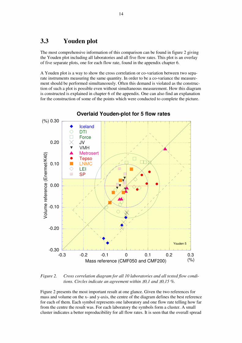
3.3 Youden plot The most comprehensive information of this comparison can be found in figure 2 giving the Youden plot including all laboratories and all five flow rates. This plot is an overlay of five separate plots, one for each flow rate, found in the appendix chapter 6. A Youden plot is a way to show the cross correlation or co-variation between two sepa-rate instruments measuring the same quantity. In order to be a co-variance the measure-ment should be performed simultaneously. Often this demand is violated as the construc-tion of such a plot is possible even without simultaneous measurement. How this diagram is constructed is explained in chapter 6 of the appendix. One can also find an explanation for the construction of some of the points which were conducted to complete the picture.

-0.30

-0.20

-0.10

0.00

0.10

0.20

0.30

-0.3 -0.2 -0.1 0 0.1 0.2 0.3

Overlaid Youden-plot for 5 flow rates

IcelandDTIForceJVVMHMetrosertTepsoLNMCLEISP

Vo

lum

e r

efe

ren

ce

(E

nerm

et/

K4

0)

Mass reference (CMF050 and CMF200)

Youden 5

(%)

(%)

Figure 2. Cross correlation diagram for all 10 laboratories and all tested flow condi-

tions. Circles indicate an agreement within ±0,1 and ±0,15 %. Figure 2 presents the most important result at one glance. Given the two references for mass and volume on the x- and y-axis, the centre of the diagram defines the best reference for each of them. Each symbol represents one laboratory and one flow rate telling how far from the centre the result was. For each laboratory the symbols form a cluster. A small cluster indicates a better reproducibility for all flow rates. It is seen that the overall spread

15

of the symbols is roughly the same in both axis directions. This is true for example the clusters from LNMC, LEI, Tepso, VMH and DTI. For SP and JV the spread concerning the mass meter is less than concerning the volume meter. For Force the opposite is true. Metrosert has one outlier as recognized by the laboratory for the highest flow rate. VMH has the lowest overall spread and is closest to the centre. Iceland (only four flow rates) finally has a negative offset with respect to both meters. It should, however, be mentioned that if K40 had been chosen as volume reference, all of Iceland’s points would have been on the upper half and much closer to the centre-line. Further to complete the picture all data for JV and 2 values for DTI were imported from the K40 measurement, which is explained in 3.6. As mentioned, the centre is defined as the reference with respect to both meters (meter combinations). The reference is not an absolute one, but the probably most relevant for this comparison treating all results equally as long as none can be regarded being an out-lier. The diagram contains a 45 ° line saying that results like one point for Metrosert is regis-tered to be systematically too high with respect to both meters. Thus results spread along this inclined line indicate systematic deviations. The rectangle shows spread of systematic character along the 45 °lines and spread of random character orthogonal to that direction. If we disregard one recognized outlying point from Metrosert and some points from Ice-land and recall that the JV points actually refer to a less stable volume reference, we can say that the total result is within 0,15 % and the clear majority of the data is within just 0,1 % from the reference for this inter-comparison.

3.4 Calibration results for the different meters The Youden plot technique is a suitable means to give a global overview, but lacks im-portant details. Those are revealed in presenting all results traditionally as error curves overlaid.

3.4.1 Mass flow meters CMF200 and CMF050 The individual results for the two coriolis meters from Micro-motion are shown in figures 3 and 4. The two meters overlap in the low flow region, where however the smaller one, CMF050, is the better choice. The graph for the CMF050 indicates varying repeatability between the laboratories. Many results are found within the repeatability (short time spread) of each other. If instead the uncertainty bars had been drawn, all would have covered the reference value (arithmetic mean) at both flow rates as a consistency check showed (se table A7 in the appendix). The graph for the CMF200 visualizes one point at the highest flow rate that was recog-nized by the laboratory to be an outlier. All of Iceland’s points are low. A consistency test performed at all flow rates showed that with the mentioned outlier the rest of the results are consistent with each other and the reference and the uncertainties given or appointed in table 5 for flow rates 5, 10 and 20 ton/h, but not for 1 and 2 ton/h. Either one of the laboratories DTI or Force fit in with respect to the claimed uncertainty. But it must be mentioned that both laboratories had a test temperature on respective side of 50 °C, i.e. not quite comparable to the reference. Due to a clearly temperature dependent zeroing effect, the CMF200 is critically sensitive in this particular temperature region (se figure A6 in appendix chapter 4).

16

-0.10

-0.05

0.00

0.05

0.10

0.15

0.20

0.5 1 1.5 2 2.5 3

Coriolis mass flow meter CMF050

Iceland

DTI

Force

JV

VMH

Metrosert

Tepso

LNMC

LEI

SP

Reference

De

via

tio

n f

rom

no

min

al

K-f

ac

tor

(%)

Flow rate (m3/h)

CMF050 all labs

Figure 3. Meter error of the CMF050. The reference is the average over all laboratories. The vertical bars represent the within-laboratory repeatability calculated according to equation (A1) in chapter 3 of the appendix..

-0.40

-0.30

-0.20

-0.10

0.00

0.10

0.20

0.30

0 5 10 15 20 25

Coriolis mass flow meter CMF200

IcelandDTIForceJVVMHMetrosert

TepsoLNMCLEISPReference

De

via

tio

n f

rom

no

min

al

K-f

ac

tor

(%)

Flow rate (m3/h)

CMF200 all labs 2

Figure 4. Meter error of the CMF200. The reference is the average over all laboratories. The vertical bars symmetric around the reference points give the inter laboratory standard deviation, i.e. the standard deviation calculated from the reported laboratory means. As a consequence of this behaviour and the better repeatability of the small coriolis meter in the low flow region, the pilot laboratory decided to combine both meters to a common

17

reference as shown in figure 5. For the construction of the reference in figure 5 this means no laboratory result was excluded in the averaging process for the four lower flow rates. The combination of the two coriolis meters in figure 5 contains all reported results with-out any temperature corrections. The legend also contains the uncertainties claimed by the participants. These numbers vary from 0,1 to 0,45 % for this meter. For a perspective of the results in relation to each other, the graph also contains informa-tion about the average repeatability denoted r1 to r5 at the five flow rates and the inter-comparison reproducibility denoted R1 to R5 both given in percent as the error itself. The graph further contains reference points being the average from all 10 laboratory results at respective flow rate (one exception mentioned) and bars indicating the inter-laboratory standard deviation (se equation (A6) in appendix chapter 3) around the mean for each flow. Graphically speaking one thus can say with twice the standard deviation most, but not all, individual points are covered. An important aspect, which is not shown graphi-cally, is whether or not the individual results also cover the reference value and preferably even all other results with their uncertainty. For several results this is not true. A test was performed as to decide if the results are consistent with each other referring to the claimed uncertainties in calibration. This is discussed in more detail in chapter 7 of the appendix and the table A7. For this test however the weighted mean is used, which differs slightly from the arithmetic average.

-0.15

-0.10

-0.05

0.00

0.05

0.10

0.15

0.20

0.25

0 5 10 15 20 25

CMF200 and CMF050 combined as one mass reference

Iceland U=0.25

DTI U=0.11

Force U=0.1

JV U=0.1

VMH U=0.25

Metrosert U=0.45

Tepso U=0.12

LNMC U=0.2

LEI U=0.11

SP U=0.1

Reference

Devia

tio

n f

rom

no

min

al K

-fa

cto

r fo

r re

sp

ecti

ve m

ete

r (%

)

Flow rate (m3/h)

Mass flow ref CMF200 & 050

r1=0.028 r

2=0.026 r

3=0.023 r

4=0.022 r

5=0.033Average laboratory repeatability (95 % level)

Betweenlaboratorystandarddeviation

+/- 0.1 %

CMF050 CMF200

R1=0.142 R

4=0.106R

3=0.115 R

5=0.136R

2=0.122

Figure 5. The error curve for a hypothetic flow meter made up of two references covering the lower and higher flow regime respectively.

0.40

0.50

0.60

0.70

0.80

0.90

1.00

1.10

1.20

0 5 10 15 20 25

Magnetic inductiv flow meter Enermet as volume reference

Iceland 0.25<U<0.3

DTI 0.1<U<0.27

Force U=0.1

JV (no data)

VMH 0.25<U<0.26

Metrosert 0.42<U<0.49

Tepso U=0.12

LNMC 0.19<U<0.21

LEI U=0.11

SP U=0.1

Reference

Devia

tio

n f

rom

no

min

al K

-fa

cto

r (%

)

Flow rate (m3/

h)

REF enermet

Betweenlaboratorystandarddeviation

+/- 0.1 %

r1=0.061 r

2=0.060 r

3=0.065 r

4=0.086 r

5=0.087

Average laboratory repeatability (95 % level)

+0.005

+0.003

+0.01

-0.004

-0.011

-0.013

R1=0.173 R

2=0.184 R

4=0.222R

3=0.215 R

5=0.187

Intercomparison reproducibility (95 % level)

Figure 6. The error curve for the Enermet-meter used as volume flow reference. The average is used as reference value

20

3.4.2 Volume flow meters Enermet and K40 The error curves in figure 6 represent the common results from 10 laboratories. The 11th point is the average error at respective flow that was calculated without the low values from Iceland, the outlier from Metrosert at 20 m3/h (no data from JV and no data from Force for 10 and 20 m3/h). Again the bars around the average used as reference indicate the inter-laboratory standard deviation (equation A6 chapter 3 in the appendix). Twice this value contains all results except the Icelandic data. Relevant average intra laboratory repeatability and inter-laboratory reproducibility values and uncertainty figures are given to relate the results to each other. Additionally a few maximum and minimum values in the low flow region have numbers indicating a correction term that might have been ap-plied due to the “off-50 °C” test condition. As can be seen these improvements are small but mean the reproducibility is even a little bit better than the calculated one given in table 4.

-1.00

-0.50

0.00

0.50

0 5 10 15 20 25

Magnetic inductive meter K40

Iceland

DTI

Force

JV

VMH

Metrosert

Tepso

LNMC

LEI

SP

Reference

Devia

tio

n fro

m n

om

ina

l K

-fa

cto

r (%

)

Flow rate (m3/h)

K40 all labs plot small

Figure 7. Error curve for Mag-meter K40 from Krohne. For comparison the repeatability

and reproducibility data at the different flow rates were: r1/R1=0,097/0,522; r2/R2=0,054/0,256; r3/R3=0,043/0,182; r4/R4=0,044/0,190; r5/R5=0,042/0,227.

The reference meter curve was constructed from the average results excluding the LNMC data as these were recognized to be non reliable due to problems with the K40 meter out-put signal. Some important points to mention are the following. The Metrosert result at 20 m3/h is here not classified as an outlier. All of the Icelandic data are above the reference curve in contrast to the other three meters. The opposite is true for all of the SP data that are found to be generally low, compared with the starting measurement not included in the com-parison. The decision to use the Enermet as the second reference meter is based on the fact that it showed a better reproducibility in the inter comparison than the K40. The values col-lected in table 4 show that RK40 is 1,16 to 4,66 times larger than REnermet whereas the re-peatability in K40 at the same time is better. Omitting the LNMC data in the inter-laboratory reproducibility for K40 leads of course to much better values but still not as good as is the case for the Enermet.

21

3.5 Uncertainty claims Comparing measurement results, especially from calibrations, does not make sense with-out relating to the expectations the laboratories have on the quality of their data. For the En-test and a consistency test these values were needed. The laboratories specified their uncertainty claims in their written calibration document sent to the pilot. These numbers are collected in table 5 Table 5 Collection of uncertainty data claimed by the participating laboratories. All

values in percent. Values in bracket appointed by the pilot laboratory. Laboratory Flow rate CMF200 Enermet K40 CMF050 LAB 1 Iceland 1

2-4 (0,30) (0,25)

(0,30) (0,25)

(0,30) (0,25)

(0,30) (0,25)

LAB 2 DTI 1 2 3 4 5

0,11 0,14 0,10 0,10 0,10

0,14 0,12 0,1

0,14 0,27

0,12 0,11 0,11 0,11 0,13

0,11 0,11

LAB 3 Force 1 - 5 0,10 0,10 0,10 0,10 LAB 4 JV 1 - 5 0,10 0,10 0,10 0,10 LAB 5 VMH 1

2 – 3 4 5

0,25 0,26 0,25 0,26 0,25

0,28 0,25 0,26 0,26

0,25 0,25

LAB 6 Metrosert 1 2 3 4 5

0,43 0,43 0,44 0,46 0,49

0,42 0,42 0,44 0,46 0,49

0,44 0,43 0,43 0,45 0,48

0,43 0,43

LAB 7 Tepso 1 - 5 0,12 0,12 0,12 0,12 LAB 8 LNMC 1

2 3 4 5

0,19 0,22 0,19 0,20 0,22

0,19 0,21 0,21 0,20 0,20

0,22 0,19 0,19 0,23 0,26

0,19 0,19

LAB 9 LEI 1 2 - 5

0,11 0,11

0,16 0,11

0,11 0,11

0,11 0,11

LAB 10 SP 1 - 5 0,10 0,10 0,10 0,10 The uncertainty data from Iceland was lacking. The figures in brackets were appointed by the pilot laboratory for the consistency test. Generally one can state that some of the labo-ratories use the same numbers regardless which meter and which flow rate is concerned. Others are very detailed on that matter. There is roughly a factor 5 between the lowest and highest claim.

3.6 Consistency test of the results The critical point in any comparison is the choice of the reference. In the instruction pro-tocol for this comparison the pilot laboratory declared to define the reference through its first and final measurement. For key-comparisons the suggested method is to build a weighted average, where the weighing is due to the uncertainty in such a way that data with low claimed uncertainty has a larger influence than those with a high uncertainty. This however would demand a clearly harmonized uncertainty declaration and the ab-sence of systematic errors. After viewing the preliminary results at a meeting at SP in December 2005 the pilot laboratory has chosen to treat all results at the different flow rates with the same weight, i.e. to use the arithmetic mean as the best reference as long as

22

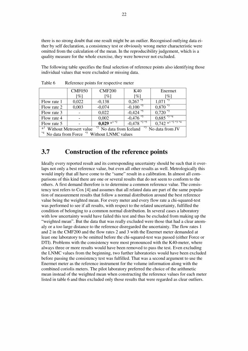
there is no strong doubt that one result might be an outlier. Recognised outlying data ei-ther by self declaration, a consistency test or obviously wrong meter characteristic were omitted from the calculation of the mean. In the reproducibility judgement, which is a quality measure for the whole exercise, they were however not excluded. The following table specifies the final selection of reference points also identifying those individual values that were excluded or missing data. Table 6 Reference points for respective meter

CMF050 [%]

CMF200 [%]

K40 [%]

Enermet [%]

Flow rate 1 0,022 -0,138 0,267 *5 1,071 *3 Flow rate 2 0,003 -0,074 -0,100 *5 0,870 *3 Flow rate 3 - 0,022 -0,424 *5 0,720 *3 Flow rate 4 - 0,002 -0,476 *5 0,685 *3 *4 Flow rate 5 - 0,029 *1 *2 -0,478 *2 *5 0,742 *1 *2 *3 *4

*1 Without Metrosert value *2 No data from Iceland *3 No data from JV *4 No data from Force *5 Without LNMC values

3.7 Construction of the reference points Ideally every reported result and its corresponding uncertainty should be such that it over-laps not only a best reference value, but even all other results as well. Metrologically this would imply that all have come to the “same” result in a calibration. In almost all com-parisons of this kind there are one or several results that do not seem to conform to the others. A first demand therefore is to determine a common reference value. The consis-tency test refers to Cox [4] and assumes that all related data are part of the same popula-tion of measurement results that follow a normal distribution around the best reference value being the weighted mean. For every meter and every flow rate a chi-squared-test was performed to see if all results, with respect to the related uncertainty, fulfilled the condition of belonging to a common normal distribution. In several cases a laboratory with low uncertainty would have failed this test and thus be excluded from making up the “weighted mean”. But the data that was really excluded were those that had a clear anom-aly or a too large distance to the reference disregarded the uncertainty. The flow rates 1 and 2 in the CMF200 and the flow rates 2 and 3 with the Enermet meter demanded at least one laboratory to be omitted before the chi-squared-test was passed (either Force or DTI). Problems with the consistency were most pronounced with the K40-meter, where always three or more results would have been removed to pass the test. Even excluding the LNMC values from the beginning, two further laboratories would have been excluded before passing the consistency test was fulfilled. That was a second argument to use the Enermet meter as the reference instrument for the volume information along with the combined coriolis meters. The pilot laboratory preferred the choice of the arithmetic mean instead of the weighted mean when constructing the reference values for each meter listed in table 6 and thus excluded only those results that were regarded as clear outliers.

23

3.8 En-value test A different test whether or not an individual calibration result is acceptable in an inter-comparison is based on the En-value. The definition is given according to (2)

( ) ( )

( ) ( )1

22≤

+

−=

jrefj

krefkj

eueu

qeqeEn (2)

The simple message of this test is that the distance of a result from laboratory j at flow rate qk from the reference value should never be so large that the respective uncertainties do not overlap. Only if this condition is fulfilled there is a small probability that the de-tected error actually could represent the reference value. A small En-value indicates a more reliable calibration result than a large one. The closeness to zero however is not only determined by the difference in the nominator. A large uncertainty in the denomina-tor also gives the impression of a good result. Thus the plane value only tells if the result is acceptable with respect to the inter-comparison reference. Only if all laboratory uncer-tainties were very similar, the En-value could be considered as a direct quality measure. Table 7 En-values for the most interesting

Mass flow meter CMF050 & 200 Volume flow meter Enermet

Flow rate Flow rate

1 2 3 4 5 1 2 3 4 5

Iceland 0,00 -0,09 -0,56 -0,32 - -0,45 -0,67 -0,89 -0,98 -

DTI -0,38 -0,07 -0,64 -0,17 -0,23 -0,12 -0,64 -0,85 -0,44 -0,39

Force 0,84 0,36 0,22 0,30 0,01 0,77 0,78 0,78 - -

JV -0,17 -1,03 -0,33 -0,02 0,01 - - - - -

VMH -0,05 -0,65 -0,33 -0,11 -0,03 0,09 -0,05 -0,04 0,00 0,04

Metrosert -0,03 0,75 -0,09 0,00 0,36 -0,14 -0,14 -0,02 -0,05 0,30

Tepso 0,98 0,49 0,19 0,75 0,35 0,06 0,06 0,32 0,42 -0,27

LNMC -0,37 0,97 -0,28 -0,13 0,10 -0,36 -0,13 -0,13 0,12 0,24

LEI -0,13 -0,56 0,12 0,26 0,02 -0,32 0,20 -0,07 -0,03 -0,28

SP -0,26 0,00 -0,40 -0,06 -0,32 0,56 0,39 0,13 0,08 -0,12

Table 7 displays only few questionable results in bold style. These are due to small uncer-tainties or large distances from the reference or both of these. Other values look OK but this is partly due to large uncertainty claims. But this is natural with definition (2) as some laboratories are not seeking for better measurement capability. In contrast to the chi-squared test, the En-value test does not describe a rigorous defini-tion of the reference value or its uncertainty. For the reference values the data in table 6 were used. The uncertainty figures are taken from table 5. The uncertainty determination of the reference is not simple. If the weighted mean were chosen, the laboratories with low uncertainty would dominate its value and even its un-certainty, which would be unrealistically low (0,02 %). On the other hand the uncertainty of the arithmetic mean is dominated by the contribution from few very large uncertainties leading to an unrealistic high value of 0,2 %. The uncertainty of the reference values are therefore based on the estimation and experience of the pilot laboratory being set to 0,08 % for both the coriolis meters and 0,1 % for the Enermet meter.

24

4 Interpretation of results and conclusions The overlaid Youden plot shows a few outlying points, but also states a rather good agreement between the laboratories. The larger circle visualizes that all “valid values” for all flow rates (dynamic range 1:20) are within a range of 0,3 %. The conclusion is that all participating laboratories in a routine like calibration only very rarely would have a meas-urement error exceeding ±0,3 % despite uncertainty claims of up to ±0,5 %. The majority of all data is actually within ±0,1 % of the chosen references. This is true for the mass flow meters and the magnetic-inductive Enermet-meter. For the Krohne meter K40 ±0,2 % (at the lowest flow rate ±0,3 %) applies. This is seen from the figures 3 to 7 and the Youden plots in the appendix – chapter 6. This is also what table 3 and 4 tell statistically, all data included. An immediate conclusion is that the laboratories, some of them participating for the first time in an inter-comparison, have demonstrated an overall agreement that is a strong sup-port for the statement that it is possible not only for one laboratory but for many to cali-brate/test class 1 heat meters. The agreement is within the demanded measurement capa-bility of ±0,2 %. The use of more than two meters is not usual in inter-comparisons, but it has some advan-tages. If there is some data missing or of limited quality it can be compensated for by redundant information. It also gives hints where to look for differences when meters seem to show different behaviour. On the other hand systematic effects that show up in several meters strengthen the suspicion. Such an aspect is the fact that the chosen references show an obvious offset for Iceland. It is acceptable with the appointed uncertainty. But there might be an interaction between the meter in question and the used method and equipment. The same is valid for the high flow for Metrosert. These details are, however, not discussed here. In general the experimental part of the inter-comparison involving ten laboratories could be accomplished within four months and gave an unexpected positive result in the good overall agreement especially in the light of the very short measurement time. But one must not forget that an important contribution to this most probably is the construction of meter package that is kept unchanged and the constant presence of the pilot.

25

5 References [1] MID directive – Directive 2004/22/EC of the European Parliament and of the

Council of 31 March 2004 on measuring instruments. [2] Lau P. and Stolt K., Calibration intercomparison of flow meters for kerosene.

Synthesis report 3476/1/0/203/92/9-BCR-S (30). SP Report 1995:77 [3] Measurement System Analysis (MSA) Reference Manual, third edition, Appen-

dix C d2 – Table with reference to Acheson Duncan, Quality Control and Indus-trial Statistics, 5th edition, McGraw-Hill, 1986.

[4] Cox M., “The evaluation of key comparison data”, Metrologia, 2002, 39, 589-595

i

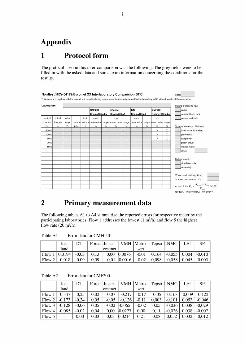
Appendix

1 Protocol form The protocol used in this inter-comparison was the following. The grey fields were to be filled in with the asked data and some extra information concerning the conditions for the results. Nordtest/NICe 04172/Euromet XX Interlaboratory Comparision 50°C Date:

This summary, together with the normal test report including measurement uncertainty, is sent by the laboratory to SP within 2 weeks of the calibration.

Laboratory: Means of creating flow:

CMF200 Enermet K40 CMF050 pump

Knom=100 p/kg Knom=720 p/l Knom=100 p/l Knom=1000 p/kg constant head tank

nominal actual water test error error error error pressurized tank

flowrate flowrate temp pressure volume mean value range mean value range mean value range mean value range

l/h l/h °C kPa l % % % % % % % % Volume reference: Metroset

20000 X X fixed volume standard

10000 X X gravimetric

5000 X X ball prover

2000 piston prover

1000 master meter

other;

Meters tested:

simultaneously

separately

Water conductivity (µS/cm):

at water temperature (°C):

range(%)= max error(%) - min error(%)

error (%) = =−

×EK K

Kxactual nom

nom

100

2 Primary measurement data

The following tables A1 to A4 summarize the reported errors for respective meter by the participating laboratories. Flow 1 addresses the lowest (1 m3/h) and flow 5 the highest flow rate (20 m³/h). Table A1 Error data for CMF050

Ice-land

DTI Force Juster-vesenet

VMH Metro-sert

Tepso LNMC LEI SP

Flow 1 0,0194 -0,03 0,13 0,00 0,0076 -0,01 0,164 -0,055 0,004 -0,010 Flow 2 -0,018 -0,09 0,09 -0,01 -0,0016 -0,02 0,098 -0,058 0,045 -0,003

Table A2 Error data for CMF200

Ice-land

DTI Force Juster-vesenet

VMH Metro-sert

Tepso LNMC LEI SP

Flow 1 -0,347 -0,25 0,02 -0,07 -0,217 -0,17 -0,05 -0,168 -0,009 -0,122 Flow 2 -0,173 -0,24 0,05 -0,05 -0,126 -0,11 0,003 -0,101 0,053 -0,046 Flow 3 -0,128 -0,06 0,05 -0,02 -0,065 -0,02 0,05 -0,036 0,038 -0,029 Flow 4 -0,085 -0,02 0,04 0,00 -0,0277 0,00 0,11 -0,026 0,038 -0,007 Flow 5 - 0,00 0,03 0,03 0,0214 0,21 0,08 0,052 0,032 -0,012

ii

Table A3 Error data for Enermet Ice-

land DTI Force Juster-

vesenet VMH Metro-

sert Tepso LMN LEI SP

Flow 1 0,924 1,05 1,18 - 1,096 1,01 1,08 0,993 1,01 1,151 Flow 2 0,687 0,77 0,98 - 0,856 0,81 0,88 0,839 0,9 0,925 Flow 3 0,475 0,60 0,83 - 0,71 0,71 0,77 0,689 0,71 0,739 Flow 4 0,419 0,61 - - 0,686 0,66 0,75 0,711 0,68 0,697 Flow 5 - 0,63 - - 0,754 0,89 0,7 0,795 0,7 0,725 Table A4 Error data for K40

Iceland DTI Force Juster-vesenet

VMH Metro-sert

Tepso LMNC LEI SP

Flow 1 0,427 0,55 0,46 0,07 0,536 0,4 -0,05 -0,741 0,09 -0,083

Flow 2 -0,077 0,01 0,03 -0,27 0,042 -0,05 -0,21 -0,714 -0,1 -0,279

Flow 3 -0,386 -0,36 -0,32 -0,55 -0,37 -0,38 -0,46 -0,71 -0,41 -0,579

Flow 4 -0,491 -0,37 -0,35 -0,61 -0,46 -0,42 -0,48 -1,139 -0,49 -0,617

Flow 5 - -0,37 -0,37 -0,60 -0,488 -0,33 -0,55 -1,203 -0,49 -0,626

3 Calculation of repeatability/reproducibility The reporting form asked for the range (maximum – minimum error) at each measured flow rate. The repeatability r is defined by equation (A1)

( )ν,

kseriesin,jd

qrr2

12 ⋅⋅= −

t (A1)

( )kseriesin,j qr −

t: The range, i.e. the difference between the highest and lowest error

e (qk) within a series of i=1 to n=5 values measured in direct succes-sion at flow rate qk.(k=1,..,5)

ν,d2 A statistical factor transforming the range into a standard deviation.

The value of d2 depends on the degrees of freedom, i.e. one less than the number of repeated measurements ν=n-1. [3]

For small sample sizes this actually is considered to be a more reliable estimate of the experimental spread than the following definition, which is equivalent.

( ) σν12 tqsr kseriesin,j ⋅⋅= − (A2)

( )kseriesin,j qs − : The experimental in-series standard deviation for laboratory j

( )( ) ( )( )

1n

qeqe

qs

n

1i

2

kjki,j

kseriesin,j−

−

=

∑=

− (A3)

( )kj qe : The average error for laboratory j at flow rate qk k=1 to 5.

( ) ( )∑=

⋅=n

i

ki,jkj qen

qe1

1 (A4)

( )ki,j qe The error found in laboratory j at run i and flow rate qk σ

ν

1t : Student t-factor giving the standard deviation for ν= n-1 repeated

measurements a stronger statistical weight on a one sigma level.

iii

Assuming normal distribution the factor 2 is in both cases chosen for expansion to a probability corresponding to 95 % confidence level. The reproducibility R is defined by equation (A5)

( ) ( )[ ]21

pklaberint

2

,2

kseriesin,j tqsd

1qr2R σ

−

ν

⋅+

⋅⋅=

t (A5)

( )klaberint qs − The inter-laboratory standard deviation, i.e. the spread between the

average errors from the l participating laboratories at flow rate qk

( )( ) ( )( )

11

2

−

−

=∑

=−

l

qeqe

qs

l

i

krefki

klaberint (A6)

( )kref qe The reference value defined as the arithmetic mean of the average

errors from all participating laboratories at flow rate qk.

( ) ( )∑=

⋅=l

j

kjkref qel

qe1

1 (A7)

Both repeatability and reproducibility are a quantitative measure for a symmetric variabil-ity around an average error. The reproducibility is the statistical combination of the in-series standard deviation from n=5 repeated runs and the standard deviation calculated from q reproduced average K-factors with p=l-1 degrees of freedom, again transformed to a 95 % confidence level. For the inter-laboratory situation l=10 and for the intra labora-tory case l=8.

4 Temperature behaviour of the meters All flow meters are sensitive for changes in medium temperature. The stipulated test tem-perature for the comparison was set to 50 °C, but almost all of the calibration results refer to slightly different values and must be checked if they can affect reported measurement data. Table A5: Deviation from stipulated test temperature 50 °C in the different laboratories.

Flow rate 1 Flow rate 2 Flow rate 3 Flow rate 4 Flow rate 5 LAB 1 Iceland 2,1 2,2 2,7 2,7 -

LAB 2 DTI 0,5 0,5 1,5 2,0 1,8

LAB 3 Force -1,6 -2,5 -2,1 -3,1 -3,9

LAB 4 JV -0,9 0,0 0,1 0,4 0,6 LAB 5 VMH -0,7 0,0 -0,2 0,1 0,2 LAB 6 Metrosert -0,2 0,9 -0,7 -0,5 4,4

LAB 7 Tepso 1,0 0,5 -0,2 -0,5 -0,6 LAB 8 LNMC 0,1 0,4 0,8 0,6 0,7 LAB 9 LEI -0,3 -0,1 0,0 0,1 0,2 LAB 10 SP2 0,4 0,3 0,3 0,1 0,1

In order to study the size of this effect and the possibility or necessity of a correction for the systematic temperature behaviour, the pilot laboratory performed several repeated measurements at different temperatures in the range from 40 to 55 °C.

iv

-0.4

-0.3

-0.2

-0.1

0.0

0.1

0.2

0 5 10 15 20 25

Coriolis meter CMF200 - Temperature behaviour

40 C

45 C

47 C

48 C

50 C /1

50 C /2

52 C

55 C

84 C

Mete

r E

rro

r (%

)

Flow rate (ton/h)

CMF200 Temperature behaviour

Fig. A1 The meter response at various temperatures between 40 and 55 °C. The

drastic shift at low flow rates is due to the zero setting of the meter which is very difficult to perform at temperatures differing from ambient conditions.

The two meters that are most important as reference are the CMF200 and the Enermet meter. The figures A1 and A 2 show the respective error curves with the medium tem-perature as parameter.

0.5

0.6

0.7

0.8

0.9

1.0

1.1

1.2

1.3

0 5 10 15 20 25

Enermet Temperature behaviour

40 C

45 C

47 C

48 C

50 C /1

50 C /2

52 C

55 C

Me

ter

Err

or

(%)

Flow rate (m3/h)

Enermet Temperature behaviour

Fig. A2 The meter response at various temperatures between 40 and 55 °C. A closer

analysis shows that there is no clear systematic behaviour as function of the temperature, which makes it difficult to find a suitable temperature correc-tion.

v

From the data behind these curves, the following graphs can be constructed and linear temperature dependence derived by fitting the data for the various flow rates.

-0.30

-0.20

-0.10

0.00

0.10

40 45 50 55 60

CMF 200 temperature dependence for 3 flow rates

Flow rate 3

Flow rate 2

Flow rate 1

y = 0.25229 - 0.0054293x R= 0.92586

y = 0.65164 - 0.013757x R= 0.8793

y = 1.207 - 0.026178x R= 0.82245

Change

in

K-f

acto

r devia

tio

n fro

m n

om

inal valu

e (

%)

Medium temperature (C)

CMF200 Tempdependence

Fig A3 The fitted lines to the data for the three lowest flow rates show the strongest

temperature sensitivities of all meters in terms of error change per tempera-ture change ∆E[%]/∆T[°C].

0.40

0.60

0.80

1.00

1.20

1.40

40 45 50 55 60

Enermet temperature dependence for 3 flow rates

Flow rate 3

Flow rate 2

Flow rate 1

y = 0.83064 - 0.0019885x R= 0.25587

y = 1.1464 - 0.0044566x R= 0.89211

y = 1.5542 - 0.0078412x R= 0.94049

Change in K

-facto

r devia

tio

n fro

m n

om

inal valu

e (

%)

medium temperature (C)

Enermet tempdependence

Fig A4 The Enermet meter reveals minor temperature sensitivity in the fitted lines. In summary there is a slight temperature dependency for all meters. But only in half of the situations a strong enough systematic behaviour (correlation coefficient > 0,6) can be stated for a fit of type E(T) = a + b*T (se figures A4 to A5). Here T is the actual tem-perature of the medium and E(T) is the error at this temperature. The coefficients b de-termine the sensitivity to temperature in the meter error, i.e. a change of ∆E [%] as result of a change in ∆T = 1 [°C]. The relevant values are collected in table A6.

vi

-0.05

0.00

0.05

0.10

0.15

40 45 50 55

CMF 050 temperature dependence for 2 flow rates

Flow rate 2

Flow rate 1

y = 0.26695 - 0.005004x R= 0.79233

y = 0.19406 - 0.0031792x R= 0.62989

Ch

ang

e in K

-fa

cto

r d

evia

tio

n fro

m n

om

ina

l valu

e (

%)

Temperatur of medium (C)

CMF050 tempdependence

Fig A5 The small coriolis meter CMF050 has even lower temperature sensitivity

and the correlation coefficient R indicates a weak dependency. Table A6: Temperature sensitivity coefficient b οf the used transfer meters.

CMF200

∆E[%]/∆T[°C]

Enermet

∆E[%]/∆T[°C]

K40

∆E[%]/∆T[°C]

CMF050

∆E[%]/∆T[°C] Flow rate 3 -0,00543 -0,00199 -0,0098 - Flow rate 2 -0,01376 -0,00446 -0,0116 -0,00500 Flow rate 1 -0,02618 -0,00784 -0,0152 -0,00318 The temperature sensitivity decreases with increasing flow rate and for the two highest flow rates no distinct behaviour (correlation coefficients 0,1 to 0,5) could be found in the measurement data. With the help of table A5 and A6 it is possible to calculate additive corrections. However, this was not done to the inter-comparison data because the changes are too small to be relevant with respect to the stated uncertainties and the reported repeatability. Table A7: Maximum possible corrections for temperature deviations.

Flow rate 1 [%] Flow rate 2 [%] Flow rate 3 [%] LAB1 Iceland +0,055 – +0,0067 +0,03 – +0,0098 0,0145 – 0,0054 LAB2 DTI -0,008 – -0,003 LAB3 Force -0,042 – -0,005 +0,034 – -0,011 -0,011 – -0,004

Table A7 specifies the largest possible corrections that could be applied for the lower flow regime. The left cell values corresponding to the CMF200 would be meaningful to correct. For the inter-comparison however the two lowest values from CMF050 were used as reference for the comparison. For these the right side values in the cells would apply. These on the other hand are not significant enough to make a correction meaning-ful. The effect of a temperature correction is however indicated in figure 6 for the Ener-met meter. The important conclusion is that no corrections were applied. One should, however, ob-serve that these would slightly reduce the reproducibility, which intuitively is expected.

vii

5 Pressure dependency A change in line pressure physically expands the meters and one would expect that a lar-ger diameter would lead to a lower K-factor, at least for the magnetic inductive meters, and thus to a reduction in meter signal. The pressure reaction of the coriolis meters is more difficult to predict. As figure A6 shows this effect can be seen for the Mag meter K40 at the lowest flow rate. A pressure rise from 1 to 5 bar, which is a drastic change, results in a 0,06 % drop. For the Enermet meter, figure A7, this effect is only half of that. At flow rate 4 this is strongly reduced. For the coriolis meters a pressure effect is hard to see.

-0.80

-0.60

-0.40

-0.20

0.00

0.20

0 2 4 6 8 10

Pressure dependence for CMF200, CMF050 and K40 at 45 C

CMF200 / 1 bar

CMF200 / 5 bar

K40 / 1 bar

K40 / 5 bar

CMF050 / 1 bar

CMF050 / 5 bar

Me

ter

Err

or

(%)

Flow rate (t/h or m3/h)

Fig A6 Test to reveal a possible pressure dependency of three meters.

0.60

0.70

0.80

0.90

1.00

1.10

1.20

0 2 4 6 8 10 12

Pressure dependence for Enermet meter at 45 C

Enermet / 1bar

Enermet / 5 bar

Me

ter

err

or

(%)

Flow rate (m3/h)

Fig A7 Pressure test at two flow rates to reveal a possible pressure dependency. The conclusion from the figures A6 and A7 is that there is no need to look for any differ-ences between the laboratories that might be related to different line pressures.

viii

6 Detailed Youden plots

-0.30

-0.20

-0.10

0.00

0.10

0.20

0.30

-0.3 -0.2 -0.1 0 0.1 0.2 0.3

Iceland

DTI

Force

JV

VMH

Metrosert

Tepso

LNMC

LEISP

Volu

me

refe

rence (

%)

Mass reference (%)

-0.30

-0.20

-0.10

0.00

0.10

0.20

0.30

-0.3 -0.2 -0.1 0 0.1 0.2 0.3

Iceland

DTI

Force

JV

VMH

Metrosert

Tepso

LNMC

LEI

SP

Volu

me r

efe

rence (

%)

Mass reference(%)

Fig A8. Flow rate 1 Fig A9. Flow rate 2

-0.30

-0.20

-0.10

0.00

0.10

0.20

0.30

-0.3 -0.2 -0.1 0 0.1 0.2 0.3

Iceland

DTI

Force

JV

VMH

Metrosert

Tepso

LNMC

LEI

SP

Vo

lum

e r

efe

rence

(%

)

Mass reference (%)

-0.30

-0.20

-0.10

0.00

0.10

0.20

0.30

-0.3 -0.2 -0.1 0 0.1 0.2 0.3

Iceland

DTI

ForceJV

VMH

Metrosert

Tepso

LNMC

LEI

SP

Volu

me r

efe

ren

ce

(%

)

Mass reference (%)

Fig A10. Flow rate 3 Fig A11. Flow rate 4

-0.30

-0.20

-0.10

0.00

0.10

0.20

0.30

-0.3 -0.2 -0.1 0 0.1 0.2 0.3

Iceland

DTI

Force

JV

VMH

Metrosert

Tepso

LNMC

LEI

SP

Volu

me r

efe

rence (

%)

Mass reference (%)

Each point has an x and y coordinate. In x-direction the differences between each laboratory result and the corresponding reference, being the aver-age for the mass flow meter combination over all labo-ratories, is plotted.

( ) ( ) n,....,jforqEn

qEn

j

reflilabreflilab 11

111 =

− ∑

=

In y-direction the corresponding differences to the volume reference is plotted.

( ) ( ) n,....,jforqEn

qEn

j

reflilabreflilab 11

1

22 =

− ∑

=

Fig A12. Flow rate 5 Construction of the Youden plot

ix

7 Consistency test results Assume the following conditions are fulfilled

• The meters are very stable • No laboratory result sustains of significant systematic errors • All calibrations are only subject to random effects • All uncertainty statements are based on a harmonized understanding • All uncertainties are correctly stated, but not equal

Then all results can be regarded to belong to the same population of calibration results (for each meter and each flow rate). This population is normally distributed and the best reference value is found by the weighted mean.

( )

( )∑

∑

=

==

q

i i

q

i i

i

ref

xu

xu

x

x

12

12

1 (A8)

with: xi: A laboratory average for one flow meter and one flow rate u(xi): The combined standard uncertainty in that laboratory result (k=1) q: The number of participating laboratories q=10 If all results xi and all uncertainties u(xi) are consistent, a Chi-squared-test can be applied to test consistency in the result. Based on the various results and their standard uncertain-ties, the reference value xref its uncertainty u(xref) and observed χ2-statistics can be calcu-lated using equation (A9).

( )( ) ( )[ ]∑

= −

−=

q

i refi

refiobs

xuxu

xx

122

2

2χ (A9)

This value can be compared with the χ2-value for p=q-1 degrees of freedom. The chi-squared-test looks at the probability to find an observed χ2-value, which is smaller than that of normal distributed values. If this probability is significant, for example larger than 5 %, the experimental values belong to the same population with a normal distribution and are thus consistent. If this is not the case, at least one of 10 values is considered not consistent and should be removed from the construction of the reference value (A8). With that value removed the consistency test is repeated. This test was suggested by Cox [4] and was performed for all meters and all flow rates according to the excel application in figure A18. Table A8: Result of consistency test

CMF200 Enermet K40 CMF050 Flow rate 1 OK –LAB 2 OK *1 OK –LAB 1, 2, 3, 5 & 10 OK Flow rate 2 OK –LAB 2 OK *1 OK –LAB 4, 7, 8 & 10 OK Flow rate 3 OK OK -LAB 2 OK –LAB 2, 3, & 8 - Flow rate 4 OK OK *2 OK –LAB 2, 3, & 8 - Flow rate 5 OK OK *2 OK –LAB, 2, 3, & 8 - *1 only 9 laboratory results, *2 only 8 laboratory results As table A8 shows, the K40 result are less reliable than the Enermet result. The consis-tency test was only OK if several laboratories were excluded. This test confirmed what the graphical result already indicated – the Enermet was the more reliable choice as the volume reference meter.

Fig A18 A chi-squared-test performed with the help of excel and the test function =CHI2FÖRD(M20;9) performed on the observed χ2−value.