Yurop Shrestha

Economics Thesis

CAPM vs. APT: An Empirical Analysis

Introduction

The Capital Asset Pricing Model (CAPM), was first developed

by William Sharpe (1964), and later extended and clarified by

John Lintner (1965) and Fischer Black (1972). Four decades after

the birth of this model, CAPM is still accepted as an appropriate

technique for evaluating financial assets and retains an

important place in both academic scholars and finance

practitioners. It is used to estimate cost of capital for firms,

evaluating the performance of managed portfolios and also to

determine asset prices. Since the inception of this model there

have been numerous researches and empirical testing to assess the

strength and the validity of the model. Several variations of the

models have been developed since then (Wei 1988, Stein, Fama &

French 1993, Merton 1973).

1

The Arbitrage Pricing Theory of Capital Asset Pricing

formulated by Stephen Ross (1976) and Richard Roll (1980) offers

a testable alternative to the CAPM. Both of these asset pricing

theories have gone through intense empirical and theoretical

scrutiny with multiple researches supporting or refuting both the

models. The purpose of this paper is to empirically investigate

the two competing theories in light of the US Stock Market in

relatively stable economic times.

The first section will look at the logic and theoretical

aspects of the competing asset pricing models. The second section

analyses and discusses the existing literature and empirical

analyses on both the theories. In the third section I explain the

data and the testing methods employed to empirically examine the

theories. The fourth section explains the results derived from

the tests. The last section includes the conclusion and discusses

the limits and implications of my research.

SECTION I: CAPM and APT

CAPITAL ASSET PRICING MODEL (CAPM)

2

Sharpe’s (1964) CAPM is built upon the model of portfolio

choice by Harry Markowitz (1959). According to his theory,

investors choose “mean-variance-efficient” portfolio. This

basically means that they choose portfolios that minimize the

variance of portfolio return, given expected return, and maximize

expected return, given variance. In addition to these

assumptions, the CAPM makes several other key assumptions. They

assume that (1) all investors are risk averse and looking to

maximize wealth in a single period and can choose portfolios

solely on the basis of mean and variance, (2) taxes and

transaction costs do not exist, (3) all investors have

homogeneous views regarding the parameters of the joint

probability distribution of all security returns, and (4) all

investors can borrow and lend at a riskless rate of interest

(Black et al. 1972).

The CAPM is an equilibrium model that explains why each

different security has its own distinct expected returns. It

provides a method to quantify the risk associated with each

asset. One key assumption of the CAPM is that it assumes that all

the diversifiable risk can be and is eliminated in an efficient 3

‘market’ portfolio. An individual security’s idiosyncratic risk

will be compensated for by another stock. So the risk associated

with each security is its systemic risk with the market. This is

measured in the CAPM by its beta (its sensitivity to the

movements in the market). There is a linear relationship between

the security’s beta and its expected returns. Formally the CAPM

equation can be written as follows

E (Ri)=Rf+βi(E (Rm)−Rf) (1)

Where,

E (Ri) = Expected return on the capital asset

Rf = Risk Free Rate (Usually of 6 month Treasury bill)

βi = beta which is the sensitivity of the expected excess asset

returns to the expected excess market returns. Formally, the

market beta of an asset i is the covariance of its return with

the market return divided by the variance of the market return.

βi=

Cov(Ri,Rm)

σ2(Rm) (2)

Rm = Expected return of the market

4

A zero beta asset in the CAPM has an expected return equal

to the risk free rate. The betas can be estimated using various

statistical and econometric techniques. The three most commonly

used techniques are the “market model” (This is the most common

one. I will be using this for my testing), Scholes-Williams, and

Dimson estimators. There are numerous advantages/benefits as

well as some flaws in all the beta estimating techniques.

Examining that fall outside the field of this paper but the

limitation section looks at the problems of the different

techniques very briefly. In order to compare the two models,

staying consistent with the estimation techniques will be

sufficient regardless of their flaws or biases.

ARBITRAGE PRICING THEORY

The APT is the alternative model for asset pricing first

developed by Ross (1976). This is a very appropriate model as it

agrees perfectly with what appears to be the intuition behind the

CAPM. It is based on a linear return generating process as a

first principle. Also it is more sophisticated that the CAPM

because it takes into account more systematic factors that might

5

be relevant. It examines other macroeconomic variables besides

the market risk, making this model more sophisticated. It

captures other factors that might have been ignored by the CAPM.

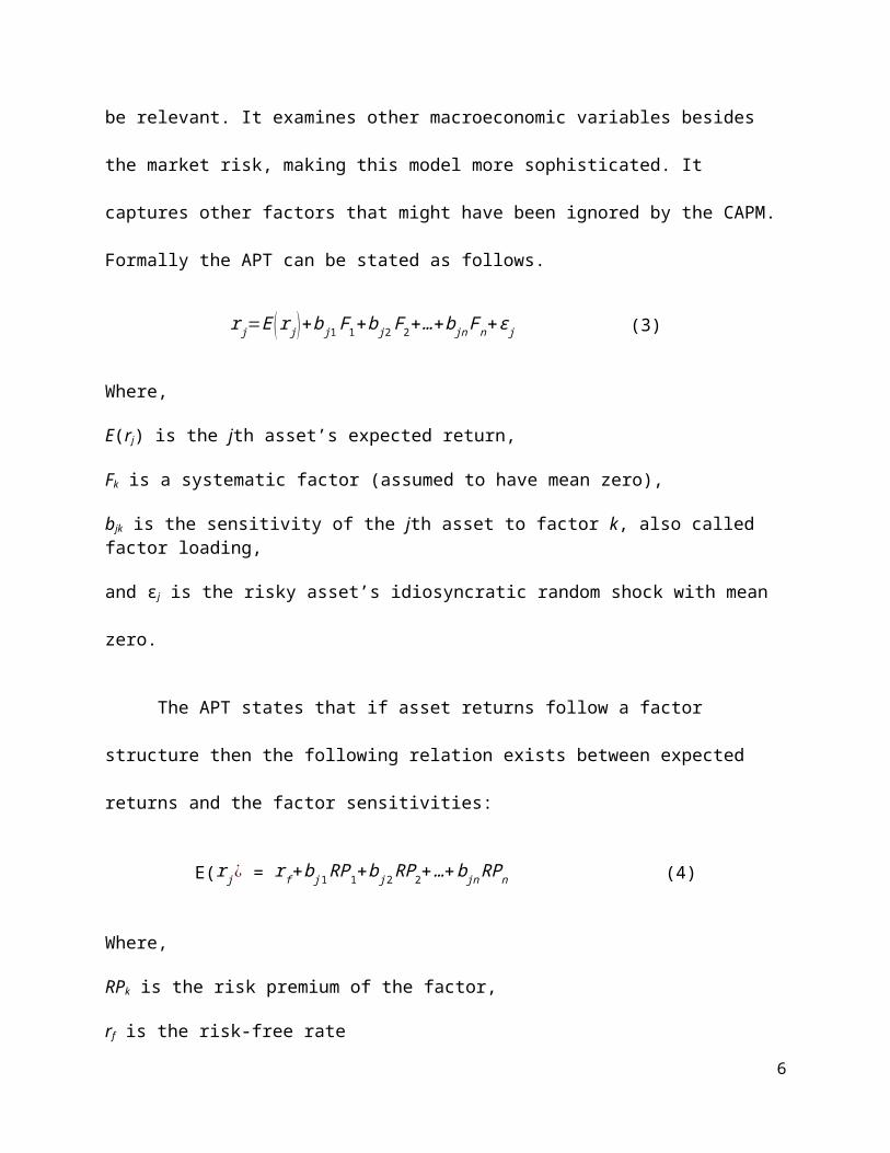
Formally the APT can be stated as follows.

rj=E (rj)+bj1F1+bj2F2+…+bjnFn+ϵj (3)

Where,

E(rj) is the jth asset’s expected return,

Fk is a systematic factor (assumed to have mean zero),

bjk is the sensitivity of the jth asset to factor k, also called factor loading,

and εj is the risky asset’s idiosyncratic random shock with mean

zero.

The APT states that if asset returns follow a factor

structure then the following relation exists between expected

returns and the factor sensitivities:

E(rj¿ = rf+bj1RP1+bj2RP2+…+bjnRPn (4)

Where,

RPk is the risk premium of the factor,

rf is the risk-free rate

6

That is, the expected return of an asset j is a linear function of the assets sensitivities to the n factors.

There are two fundamental differences between the APT and

the CAPM – “Firstly, the APT allows more than just one generating

factor (CAPM allows only for the market factor) and secondly, the

APT demonstrates that since any market equilibrium must be

consistent with no arbitrage profits, every equilibrium will be

characterized by a linear relationship between each asset’s

expected returns and its return’s response amplitudes of loadings

on the common factor” (Roll and Ross 1980). It is important to

note that the APT is based on three key assumptions – (1) Capital

markets are perfectly competitive, (2) Investors always prefer

more wealth to less wealth with certainty, (3) the stochastic

process generating asset returns can be represented as a k-factor

model of the form specified above in equation 3 (Reinganum 1981),

(4) individuals agree on both the factor coefficients (beta) and

the expected returns, (5) equation 3 not only describes the ex-

ante individual perceptions of the returns process but also that

ex-post returns are described by the same equation (Roll & Ross

1980). There are other theoretical differences between the two

7

models but a more thorough theoretical analysis falls outside the

scope of this paper and is an area of research that has been

extensively scrutinized as well.

SECTION II: LITERATURE REVIEW

There has been numerous studies theoretical and empirical

testing on both CAPM and the APT because of its high relevance in

the finance industry. This section is divided into two sub

sections – (a) Studies on CAPM, (b) Studies on APT, and (c)

Comparative studies on CAPM Vs APT. The second and the third

subsection intersect with each other. Because APT was developed

in response to the CAPM, lots of tests on APT look at it from a

comparative perspective.

A. Studies on CAPM

Although, the Sharpe (1964) and Lintner (1965) version of

CAPM has been a major theoretical force, it has not been an

empirical. Most tests of the CAPM are based on three implications

of the relationships between the expected return and the market

beta of the security – (i) Betas and the expected returns are

linearly related and no other variable has explanatory powers,

8

(ii) beta premium is positive (this also implies that higher

betas means higher returns) and (iii) assets uncorrelated with

the market have the same expected returns as the risk free rate (

Rf) (Fama & French 2004). Although the CAPM is challenged by many

studies, the influences of some earlier studies still remain and

the beta is still considered to be an important variable in the

pricing and evaluating of assets (especially in the context of an

efficient portfolio). It is important to note here that all the

studies examined below uses some sort of portfolio allocation to

test for risk-return relationships.

Fama and Macbeth (1973) tests the relationship between

average returns and risk for New York Stock Exchange (NYSE)

common stocks (from 1935 – 1968). They employ the “two-parameter”

portfolio model and models of market equilibrium derived from

that model to test for three main hypotheses of the CAPM. They

test for the relationship between the expected return on a

security and its risk in any efficient portfolio and find a

statistically significant positive linear relationship as implied

by the model. They also find that no other measure of risk in

9

addition to the portfolio risk, systematically affects the

expected returns of the security (beta is the only explanatory

variable). And they find via residual analysis that the risk-

return regressions are consistent with an efficient capital

market – a market where prices of securities fully reflect the

available information. Black, Jensen, and Scholes (1972) provide

some additional testing of the model in the same time period

(1926 – 1966) for NYSE listed common stocks as well. It corrects

some of the previous testing problems by using more powerful

time-series testing as opposed to just cross-sectional tests and

eventually comes up with a two factor model using both cross

sectional and time-series testing. They also modify the original

CAPM model by relaxing the assumption of riskless borrowing and

lending opportunities and hence strengthening the model. The

conclusions and results of their test confirm the positive linear

relationship of the beta and the expected returns of the stock

but differ with Fama and Macbeth’s conclusion regarding the

intercept of the CAPM linear regression. Both these studies

provide empirical evidence supporting the CAPM.

10

Since the earlier studies, more empirical research has shown

how the CAPM does not fairly represent the risk return

relationship it implies. Basu (1977) evaluates the investment

performance of common stocks in relation their price-earnings

ratio. He uses the CAPM model, holding beta constant to see if

the P/E ratios of the security contribute towards the expected

return. He finds that there is a higher return for assets with

lower P/E when beta is held constant. An implication of his

result poses a serious challenge to the validity of the Capital

Asset Pricing Model. Because CAPM says that there is no other

risk present in the stock when it is put in the portfolio (since

all diversifiable risks are eliminated), no other factor besides

the market risk should be present. Basu (1977) finds that P/E

ratios also influence the price, not just the market risk. The

model fails to completely characterize the equilibrium risk-

return relationship during the period he studied (NYSE firms from

1956 – 1971). It also implies that the CAPM might be mis-

specified because of the omission of other relevant factors.

Cheng and Grauer (1980) provide an alternative test to the CAPM.

They address the ambiguity in previous tests of CAPM (Roll 1977)

11

which primarily examined the security market line to look at the

risk-return relationships by employing the Invariance Law test.

Although this is not as intuitively pleasing as the standard SML

tests, it addresses the ambiguity problems with them. Their

results strongly reject the CAPM on many grounds. They find

statistically significant trends in estimated values of the

intercept as regressors are added (CAPM implies a static

intercept – the risk-free rate). They fail to reject the null

hypothesis that the beta is statistically different from zero in

25% of the cases. Their new frame work of testing further

challenges the empirical validity of the CAPM. Reinganum (1981)

further investigates whether securities with different estimated

betas systematically experience different average rates of

returns. In his study, he uses all the three beta estimation

techniques to construct his beta ranked portfolios (market model,

Sholes-Williams, and the Dimson estimator). The limitations of

the beta estimation methods are discussed in the limitations

section below. The data he looks at is the NYSE common stocks

daily and monthly returns from 1935 to 1979. His results also

show that there is no positive relationship between the firms or

12

the portfolios’ beta and the mean returns on a statistically

significant level. This result holds true regardless of the beta

estimation technique used and for both daily as well as monthly

returns. This research provides further evidence against the

empirical validity of the CAPM.

B. Studies on APT

There have been a number of studies testing the empirical

validity of the APT since its inception. One of the first studies

that tests the APT empirically was by Roll and Ross (1982). They

look at individual securities from 1962 to 1972 listed in the

NYSE or American Exchanges. They perform the maximum likelihood

factor analysis to determine the no. of factors and the

corresponding factor analysis. And then, they perform a cross-

sectional analysis using general least squared regressions. The

cross sectional part of this testing and portfolio allocations is

very similar to most of the tests on CAPM. Their research finds

four important systemic factors influences the return of a

particular security – (1) Unanticipated Inflation, (2) changes in

levels of industrial production (3) shifts in risk premiums, and

13

(4) movement in the shape of the term structure of interest

rates. They find that betas are statistically significant and

have explanatory effects on excess returns. This also empirically

proves the linear relationship between the returns and the

systemic factors. This study however recognizes that its test is

still a weak one and further testing is needed. Tϋrsoy, Gϋnsel

and Rjoub provide some further empirical tests of the Arbitrage

Pricing Theory. They examine 13 macroeconomic variables (factors)

on 11 different industry portfolios of the Istanbul Stock

Exchange (2000 – 2005) to observe the effects of those variables

on stock’s returns. They employed the ordinary least square (OLS)

technique to do this. Although they do not find strong R2 for any

of the portfolios (R2 ranges from .19 to .36), they do find a lot

of variables to be statistically significant in different

portfolios. For example they find unemployment rates to be

significant in the portfolios of manufacturing of basic metal

industry, wood production and furniture, fabric metal products,

transportation and communication. Because of the large no. of

variables employed and the inconsistencies in statistical

14

significance of the different betas in different portfolios, this

does not tell us much about the strength of the APT.

Poon and Taylor (1991) use the same methods employed by Chen,

Roll and Ross (1986) to reconsider their results and also to see

if their results were applicable to the UK Stocks. They find that

variables similar to those of the Roll and Ross tests do not

affect share prices in the UK in the manner described. They

conclude that it could be that other macroeconomic variables are

at work or the methodology of the tests employed by Ross and Ross

is inadequate for detecting such pricing relationships. They also

note some important criticism about the methodology used by Ross

and Roll. Firstly, it challenges the assumption that market

prices assets in a precise, systematic, linear manner even though

the exposure of the stock returns to the macroeconomic factors

might not be statistically significant. Secondly, it notes that

the two step regression analysis is sensitive to the number of

independent variables in the regression – adding more variables

results in loss of statistical significance of previous betas.

Thirdly, it notes that Ross and Roll did not consider any

lead/lag relationships between the asset pricing and the 15

macroeconomic performance. Fourthly, Roll and Ross fail to remove

any seasonality associated with associated with the industrial

production series. This study provides some empirical evidence

that invalidates the Arbitrage Pricing Theory by showing how the

factors found to be relevant and influential in Ross and Roll’s

(1980) study are not statistically significant when applied to

the UK Stocks – the betas associated with those macroeconomic

factors are statistically insignificant. Reinganum (1980) provide

some more empirical results of the Arbitrage Pricing Theory. He

argues that a minimum requirement for an alternate model of

capital asset pricing (CAPM) should be that it explains the

empirical anomalies which arise within the sample CAPM. One such

anomaly he observes is when portfolios are formed on the basis of

firm size; small firms systematically experience average rates of

returns nearly 20% more per year than those of large firms. He

looks at the stock data (NYSE and American Exchanges) from 1962

to 1978 to investigate whether an APT model can account for the

differences in the average returns between small firms and large

firms. He uses a three, four and a five factor model of APT to

conduct these tests and finds that none of those models accounts

16

for the empirical anomalies that arise within the CAPM. However,

he does point out that although the results do not support the

APT, the source of error can be attributed to other factors.

Regardless of that, his tests show that APT is not an adequate

model to determine the risk-return equilibrium in a statistically

significant level.

C. Comparative Studies on APT Vs CAPM

Bower, Bower & Logue (1984) look at the utility stocks in the

NYSE and American Stock exchanges from 1971 to 1979. They used

Ross & Roll’s four factors as its systematic influences. They

performed time-series analysis and cross sectional regressions to

find the betas and the risk premiums associated with each factor

to eventually come up with a multiple regression linear model

reflecting the risk-return relationship. They also find the

market beta and the security market line for the same securities

(CAPM risk-return equation). They find two very contrasting sets

of results from the two models. They found that APT to be a

better model than the CAPM. The R2 for the APT was higher for all

the portfolios when randomly grouped, when grouped by industry

17

and when grouped by market beta as well. The unexplained

variances were higher for CAPM in all the portfolios as well.

They also perform a weak Theil’s U2 and find the APT’s U2 to be

much lower than CAPM (the lower the U2, the better forecaster the

model is). This paper provides strong empirical evidence in favor

of APT when compared to the CAPM model.

SECTION III: METHODOLOGY

DATA

The data I look are all United States data from 1980 – 1997

(monthly). I chose this time period because there were no

significant long term shocks in the market or the economy during

this time. The stock market crash of 19th October 1987 is an

exception but the market recovered relatively fast and there were

no significant long term macroeconomic changes. Also, I chose

this time period because it is the most recent period

experiencing relative stability in the financial markets. There

was the dot com bubble 1997, recession after 9/11 in 2001 and the

financial crisis at 2008. A look at the S&P graph below (figure

1) shall demonstrate that.

18

Figure 1: S&P 500 Index (1975-2006)

I looked at monthly prices and returns for 160 companies

from the S&P 500. I use the adjusted data for this purpose. I

chose adjusted closing prices and not the nominal closing prices

because the adjusted closing price accounts for any corporate

actions that might change the price dramatically. For example a

2:1 stock split would half the price of the stock in a day and

subsequently distort my results.

16 companies were chosen randomly from each industry

groups. The industry groups were Energy, IT, Industrials,

Materials, Utilities, Consumer Discretionary, Consumer Staples,

Financials, Telecommunication, and Healthcare. The other

variables were inflation, changes in the term structure of

19

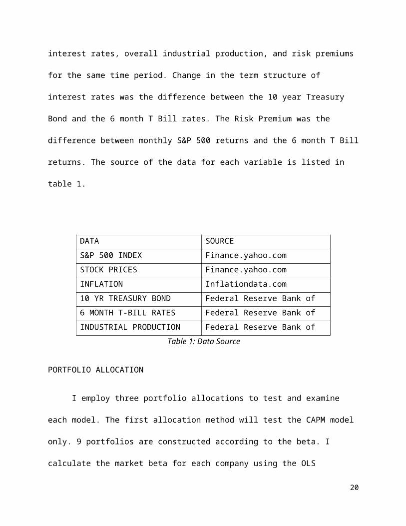
interest rates, overall industrial production, and risk premiums

for the same time period. Change in the term structure of

interest rates was the difference between the 10 year Treasury

Bond and the 6 month T Bill rates. The Risk Premium was the

difference between monthly S&P 500 returns and the 6 month T Bill

returns. The source of the data for each variable is listed in

table 1.

DATA SOURCES&P 500 INDEX Finance.yahoo.comSTOCK PRICES Finance.yahoo.comINFLATION Inflationdata.com10 YR TREASURY BOND

RATES

Federal Reserve Bank of

St. Louis 6 MONTH T-BILL RATES Federal Reserve Bank of

St. LouisINDUSTRIAL PRODUCTION Federal Reserve Bank of

St. LouisTable 1: Data Source

PORTFOLIO ALLOCATION

I employ three portfolio allocations to test and examine

each model. The first allocation method will test the CAPM model

only. 9 portfolios are constructed according to the beta. I

calculate the market beta for each company using the OLS

20

regression method and then rank the companies according to their

beta. Portfolio 1 has the lowest beta and Portfolio 9 has the

highest beta. The average betas for each portfolio can be seen in

Table 2.

PORTFOLIO 1 2 3 4 5 6 7 8 9AVG. BETA 0.364 0.91 1.177 1.652 2.018 2.535 2.82 3.585 5.155

Table 2: Portfolio Allocation I

According to CAPM, securities with different betas

systematically experience different average returns. Higher betas

would yield higher average returns (Reinganum, 1981). This is the

relationship I will be testing in the Portfolio Allocation I. I

would expect to find a statistically significant positive

relationship between beta levels of the portfolio and the average

returns. The first allocation will not be testing the APT.

In Portfolio Allocation II, I constructed ten industry

portfolios. There are 16 companies in each portfolio. I perform

an OLS test for each portfolio to find the market betas (for

CAPM) and betas for the 4 factors of APT. The four factors I

chose are inflation, risk premium, industrial production and

changes in term structure of the interest rate. I chose these 21

factors because they were the most influential factor Roll and

Ross (1980) found in their factor analysis. I looked at the

statistical significance of the betas of each factor to see how

valid APT was. Finding statistical significant betas for APT

implies that CAPM is not adequate. This is because according to

CAPM, there is no other systemic risk besides the market risk. Or

in other words, no other systematic factors affect the prices and

subsequently the returns of the stock. I also looked at R squares

for both the models to examine which model was a better fit or

which model explained the variance better.

In Portfolio Allocation III, I constructed ten random

portfolios. Each security was given assigned a random number and

then sorted accordingly. I performed the same kinds of testing

employed in Portfolio Allocation II and looked at the same

variables. This method would help eliminate any systematic bias

the industry that the stock belonged to would have on the stock

returns. This method of portfolio allocation is used in many

studies examining the two models (Reinganum (1981), Dhankar

(2005), Tursoy, Gunsel, Rjoub (2008), Black, Jensen, and Scholes

(1972)). 22

SECTION IV: RESULTS

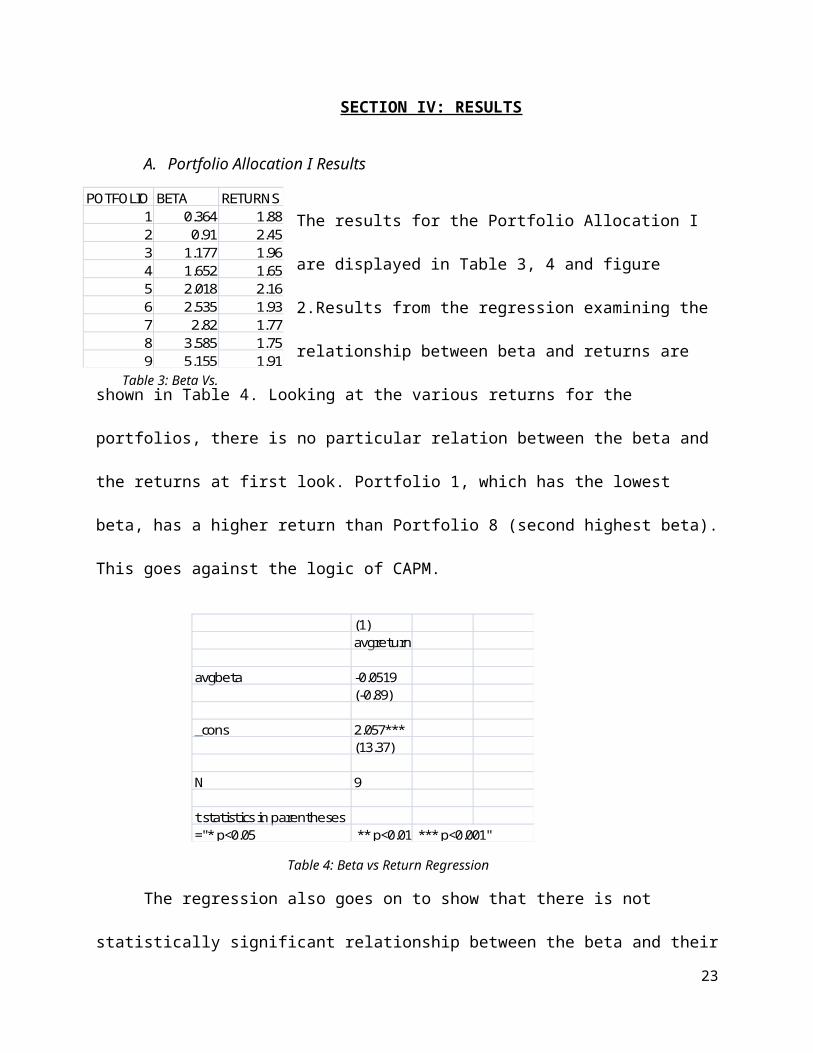
A. Portfolio Allocation I Results

The results for the Portfolio Allocation I

are displayed in Table 3, 4 and figure

2.Results from the regression examining the

relationship between beta and returns are

shown in Table 4. Looking at the various returns for the

portfolios, there is no particular relation between the beta and

the returns at first look. Portfolio 1, which has the lowest

beta, has a higher return than Portfolio 8 (second highest beta).

This goes against the logic of CAPM.

(1)avgreturn

avgbeta -0.0519(-0.89)

_cons 2.057***(13.37)

N 9

t statistics in parentheses="* p<0.05 ** p<0.01 *** p<0.001"

Table 4: Beta vs Return Regression

The regression also goes on to show that there is not

statistically significant relationship between the beta and their

23

POTFOLIO BETA RETURNS1 0.364 1.882 0.91 2.453 1.177 1.964 1.652 1.655 2.018 2.166 2.535 1.937 2.82 1.778 3.585 1.759 5.155 1.91

Table 3: Beta Vs.

returns as advocated by CAPM. A look at a simple scatter plot

(Figure 2)also shows how there is no real trend/relationship

between the beta and the return and if there is one, it is a

negative one. The first portfolio allocation test shows that

CAPM’s market beta does not determine the returns that the

security will experience.

0 1 2 3 4 5 60

1

2

3Beta Vs. Return

return

Beta

Returns

Figure 2: Beta vs. Returns Scatter Plot

B. Portfolio Allocation II Results

Results for Portfolio Allocation II are as follows. Table 5

displays the regression results for APT, Table 6 displays the

regression results for CAPM and Table 7 displays the R squares

for both the models.

24

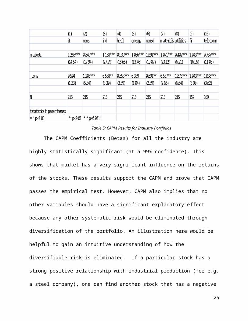
(1) (2) (3) (4) (5) (6) (7) (8) (9) (10)it cons ind heal energy consd m aterials utilities fin telecom m

m arketr 1.265*** 0.849*** 1.138*** 0.939*** 1.006*** 1.091*** 1.071*** 0.402*** 1.043*** 0.737***(14.54) (17.94) (27.79) (18.65) (13.46) (19.87) (23.12) (6.21) (16.95) (11.08)

_cons 0.504 1.205*** 0.588** 0.853*** 0.339 0.691** 0.537** 1.875*** 1.043*** 1.038***(1.33) (5.84) (3.30) (3.89) (1.04) (2.89) (2.66) (6.64) (3.90) (3.62)

N 215 215 215 215 215 215 215 215 157 169

t statistics in parentheses="* p<0.05 ** p<0.01 *** p<0.001"

Table 5: CAPM Results for Industry Portfolios

The CAPM Coefficients (Betas) for all the industry are

highly statistically significant (at a 99% confidence). This

shows that market has a very significant influence on the returns

of the stocks. These results support the CAPM and prove that CAPM

passes the empirical test. However, CAPM also implies that no

other variables should have a significant explanatory effect

because any other systematic risk would be eliminated through

diversification of the portfolio. An illustration here would be

helpful to gain an intuitive understanding of how the

diversifiable risk is eliminated. If a particular stock has a

strong positive relationship with industrial production (for e.g.

a steel company), one can find another stock that has a negative

25

relationship with industrial production (unemployment insurance

company etc). This will cancel out the systemic influence that

industrial production might have on the asset of the price of a

particular security when it is grouped in the single portfolio.

Looking at the APT results (Table 6), we find that there is

in fact other variables that statistically influences the returns

of the stocks.

(1) (2) (3) (4) (5) (6) (7) (8) (9) (10)it cons ind heal energy consd m aterials utilities fin telecom m

indprod -0.207*** -0.166*** -0.186*** -0.169*** -0.143** -0.170*** -0.242*** -0.171*** -0.0548 -0.149**(-3.74) (-5.00) (-6.38) (-5.01) (-3.02) (-4.46) (-8.08) (-4.13) (-1.29) (-3.20)

riskp -1.141*** -0.720*** -1.002*** -0.827*** -0.926*** -0.952*** -0.966*** -0.304*** -1.010*** -0.666***(-14.23) (-14.98) (-23.68) (-16.96) (-13.49) (-17.28) (-22.27) (-5.08) (-16.01) (-9.85)

term struc -0.757 -1.162*** -0.613** -1.566*** -1.237** -0.976** -0.985*** -0.987** -0.729* -0.629(-1.73) (-4.44) (-2.66) (-5.90) (-3.31) (-3.25) (-4.17) (-3.03) (-2.24) (-1.73)

infl 0.198 0.140 0.500*** 0.166 0.362* 0.398** 0.133 -0.0183 0.741** 0.438(1.02) (1.20) (4.90) (1.41) (2.19) (3.00) (1.26) (-0.13) (2.70) (1.42)

_cons 21.82*** 18.02*** 18.03*** 19.17*** 16.31*** 17.90*** 23.40*** 16.35*** 9.305** 14.33***(4.85) (6.68) (7.59) (7.01) (4.23) (5.79) (9.60) (4.87) (2.64) (3.64)

N 215 215 215 215 215 215 215 215 157 169

t statistics in parentheses="* p<0.05 ** p<0.01 *** p<0.001"

Table 6: APT Results for Industry Portfolios

26

For the IT portfolio, the betas for the risk premium

and the industrial production factors are significant. This means

that those variables have explanatory effects on the stock

returns. For the Consumer Staples portfolio, all the factors

except inflation have a statistically significant explanatory

effect. A look at the results will show industrial production has

a significant coefficient in all ten portfolios, risk premium in

all ten portfolios as well. Changes in term structure have a

statistically significant coefficient in eight out of the ten

portfolios and inflation in four out of the ten portfolios. These

results provide empirical evidence for the validity of APT. It

shows how different macro economic factors have a statistically

significant influence on the returns of the stock. An implication

of this result is that CAPM is not adequate since it finds that

there are other kinds of risk besides the market risk.

I looked at the R squares of the two models to see which

model does a better job explaining or accounting for the

variances in the return. Table 7 lists the R squared for the

different portfolios.

27

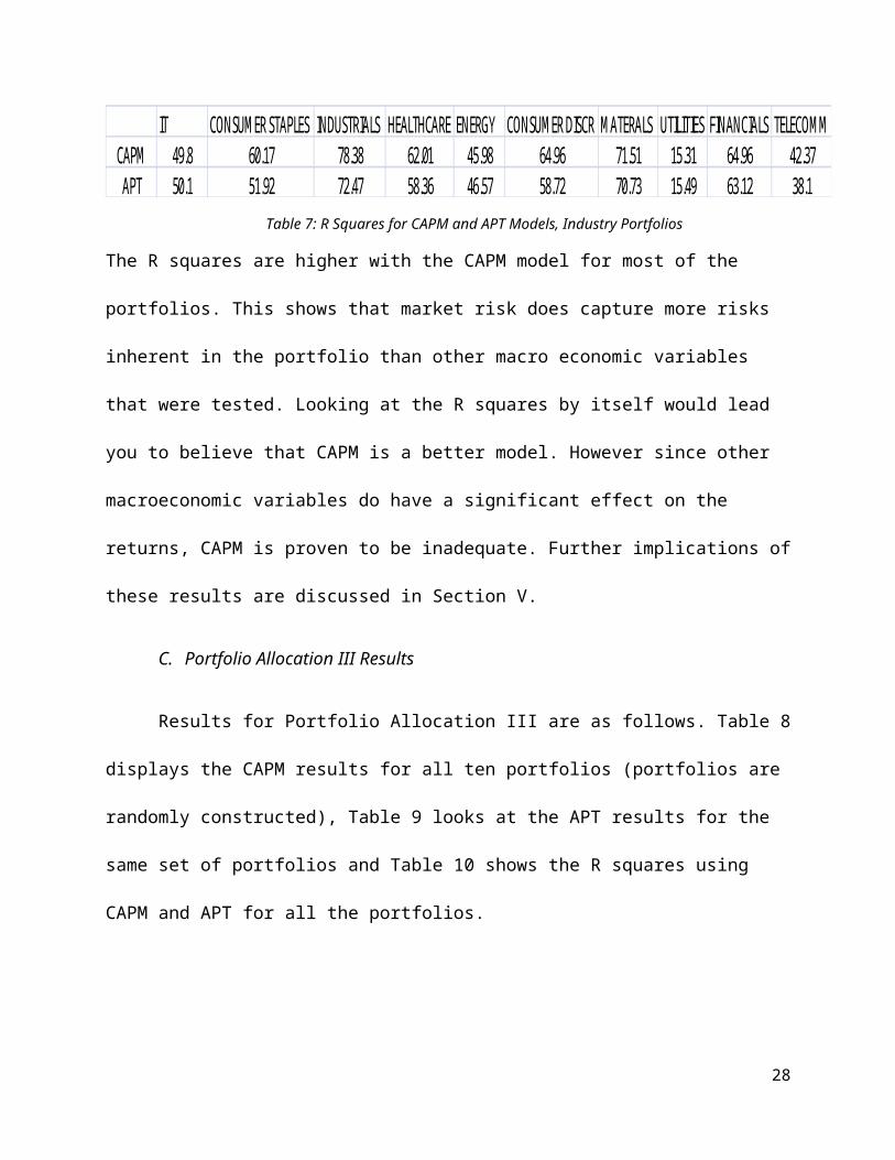
IT CONSUM ER STAPLES INDUSTRIALS HEALTHCARE ENERGY CONSUM ER DISCR M ATERALS UTILITIES FINANCIALS TELECOM MCAPM 49.8 60.17 78.38 62.01 45.98 64.96 71.51 15.31 64.96 42.37APT 50.1 51.92 72.47 58.36 46.57 58.72 70.73 15.49 63.12 38.1

Table 7: R Squares for CAPM and APT Models, Industry Portfolios

The R squares are higher with the CAPM model for most of the

portfolios. This shows that market risk does capture more risks

inherent in the portfolio than other macro economic variables

that were tested. Looking at the R squares by itself would lead

you to believe that CAPM is a better model. However since other

macroeconomic variables do have a significant effect on the

returns, CAPM is proven to be inadequate. Further implications of

these results are discussed in Section V.

C. Portfolio Allocation III Results

Results for Portfolio Allocation III are as follows. Table 8

displays the CAPM results for all ten portfolios (portfolios are

randomly constructed), Table 9 looks at the APT results for the

same set of portfolios and Table 10 shows the R squares using

CAPM and APT for all the portfolios.

28

(1) (2) (3) (4) (5) (6) (7) (8) (9) (10)rand1 rand2 rand3 rand4 rand5 rand6 rand7 rand8 rand9 rand10

sp500 0.994*** 1.140*** 0.913*** 0.970*** 0.921*** 0.919*** 0.929*** 0.669*** 1.098*** 1.018***(25.05) (25.94) (26.64) (28.21) (24.43) (24.93) (24.12) (14.00) (19.63) (13.12)

_cons 0.437* 0.781*** 0.730*** 0.705*** 1.007*** 0.558*** 0.624*** 1.422*** 1.415*** 1.475***(2.53) (4.08) (4.88) (4.71) (6.13) (3.47) (3.72) (6.83) (5.80) (4.36)

N 215 215 215 215 215 215 215 215 215 215

t statistics in parentheses="* p<0.05 ** p<0.01 *** p<0.001"

Table 8: CAPM Results for Random Portfolio Allocation

The results from the CAPM regressions for all ten portfolios

are statistically significant at a very high level (99%). These

results are similar to the ones found in the industry portfolios.

It provides further evidence that market betas are significant

even when the industry bias is removed. In other words, market

risk is reflected in the returns of the portfolios. However for

CAPM to hold ground based on empirical evidence, APT should be

shown as statistically insignificant. There should be no other

explanatory variable or no other systematic risk that affects the

returns of the portfolio. The APT results are shown below.

29

(1) (2) (3) (4) (5) (6) (7) (8) (9) (10)rand1 rand2 rand3 rand4 rand5 rand6 rand7 rand8 rand9 rand10

indprod -0.190*** -0.218*** -0.169*** -0.199*** -0.181*** -0.170*** -0.162*** -0.153*** -0.137*** -0.195***(-6.51) (-7.03) (-7.08) (-8.08) (-7.15) (-6.53) (-6.08) (-4.90) (-3.76) (-3.90)

riskp -0.856*** -1.006*** -0.808*** -0.852*** -0.826*** -0.799*** -0.824*** -0.579*** -0.986*** -0.904***(-20.23) (-22.46) (-23.36) (-23.89) (-22.60) (-21.21) (-21.32) (-12.79) (-18.73) (-12.48)

term struc -0.968*** -1.341*** -1.093*** -0.969*** -1.219*** -0.732*** -0.972*** -1.109*** -1.012*** -1.127**(-4.20) (-5.49) (-5.80) (-4.99) (-6.12) (-3.57) (-4.62) (-4.49) (-3.53) (-2.86)

infl 0.198 0.188 0.0948 0.114 0.266** 0.0899 0.269** 0.212 0.667*** 0.549**(1.94) (1.74) (1.13) (1.33) (3.02) (0.99) (2.89) (1.94) (5.25) (3.14)

_cons 19.08*** 22.86*** 18.42*** 20.21*** 18.95*** 17.60*** 17.00*** 16.00*** 15.70*** 19.44***(8.04) (9.09) (9.49) (10.10) (9.24) (8.32) (7.83) (6.29) (5.31) (4.78)

N 215 215 215 215 215 215 215 215 215 215

t statistics in parentheses="* p<0.05 ** p<0.01 *** p<0.001"

Table 9: APT Results for Random Portfolio Allocation

The results indicate that industrial production, risk

premium and changes in term structure have statistically

significant betas in all the portfolios. The beta for inflation

is statistically significant in four out of the ten portfolios.

These results provide empirical evidence for the validity of the

APT. It also implies that CAPM is not adequate as it fails to

take into account some of the other macroeconomic risks. These

30

result shows that market risk is not the only variable that

influences returns as implied by the CAPM.

1 2 3 4 5 6 7 8 9 10CAPM 74.66 75.96 76.92 78.88 73.69 74.48 73.2 47.93 64.41 44.69APT 66.24 70.74 72.48 73.42 71.03 68.81 68.41 45.18 63.07 43.58

Table 10: R Squares for CAPM and APT Models, Random Portfolio Allocation

The R squared is slightly higher when CAPM is employed as

opposed to the APT. This result is again congruent with the ones

found in the industrial portfolios. It shows how the market

overall explains the variances better than other macroeconomic

factor. Looking at the R squares might show that CAPM is a better

model. However, as mentioned earlier, R squares do not capture

the whole picture. Implications of these results are discussed

below.

SECTION V: IMPLICATIONS, LIMITATIONS, AND CONCLUSION

A. Implication

The results shown above demonstrate a couple of things about

each model. The first results from portfolio allocation prove

that beta does not determine the returns. It provides empirical

evidence refuting the CAPM theory. Although CAPM is falsified in

31

the first test, the other two tests (Portfolio Allocation I and

II) show that market risk is significantly reflected in the asset

returns. The testing for APT in these two tests shows that other

macroeconomic risks are also reflected in the stock return. The

two models cannot both be correct because CAPM says that only

market risk is evident in the asset and no other systematic risk

variable exists. Statistically significant betas for APT in both

the portfolio allocation tests show that there are other

macroeconomic variables that account for the returns of the

security, proving CAPM inadequate. The better R squares for CAPM

shows that market risks and movements explain the variance in the

stock returns better than all the macroeconomic factors in the

APT model. Although it explains the variance better, it ignores

other significant risks present in the stock returns. This can be

problematic when calculating the stock price and making

investment decisions.

These results show that the APT might have a slight edge

over the CAPM just because it is not falsified and the results

for it were statistically significant. However it’s weaker R

squared values (although not significantly weaker) show that it 32

cannot explain the variances in the returns as well as the CAPM

can. Financial practitioners should use both the models in

junction and not choose one over the other. Although my results

show APT is stronger and CAPM is inadequate, CAPM’s better R sq.

and the statistical significance of its betas should not be

ignored.

B. Limitations

There are some limitations in this whole research one must

keep in mind. Overcoming these limitations will strengthen the

research but the results of the tests I have done are still valid

and provide insightful empirical evidence that has serious and

meaningful implications. The first big limitation of this paper

is the lack of econometric sophistication. For example the use of

more complicated model than the OLS regression model like the

GARCH would give more accurate results. It would account for the

noise present in the financial data. Also for my APT testing, I

use Ross & Roll’s (1980) factors. I could perform my own factor

analysis to come up with the macroeconomic variables relevant for

my data which would strengthen my APT results. Again, due to lack

33

of my sophistication in econometrics and Stata, I could not use

this step. However, these macroeconomic factors (inflation,

industrial production, changes in term structure, risk premiums)

are used in other studies too (Poon & Taylor, 1991) and still

present valid evidence for the strength of the model.

Another limitation of my paper is the beta estimation

technique I use, specially for the CAPM models. I use the time

series OLS regression to estimate betas (this is the market

model). Using the market model estimator might be problematic for

daily returns of nonsynchronous trading problems. And if

nontrading is a serious problem this might lead to biases in the

estimation which would affect the results (Reinganum, 1981).

Other two estimation methods are However, even the Scholes

Williams estimator might be biased and inconsistent if nontrading

is a serious enough problem according to Dimson. Using all three

estimation techniques would have led me to come to a conclusive

answer; my answer is limited only to the market model. The bias

evident in the market model estimating technique is present in my

results and should be eliminated by using these other estimation

method. 34

On a broader perspective, my research looks at stock market

data for a very specific time period. The external validity of

this research is only application to developed stock markets

during times of stability. The findings of this paper would not

be applicable to developing stock markets or when the stock

market demonstrates extreme volatility or experiences other kinds

of exogenous or endogenous shocks. In the real world, markets

experience these fluctuations, hence lays my biggest limitation.

There has not been enough testing of these models for times of

crisis and shocks in the financial markets. This is an area where

more empirical analysis and testing are warranted.

C. Concluding Remarks

The results have shown that both models are not perfect. APT

is better because it takes into account systematic risks other

than the market risk as opposed to the CAPM which just accounts

for the market risk. The empirical validity of the APT refutes

the adequacy of CAPM as an asset pricing model. But the greater R

squared demonstrated by the CAPM should not be forgotten as well.

The risk averse and the rational investor would benefit using

35

both models and coming to the most sound decision. Market risks

should not be ignored but neither should other macroeconomic

risks. Further research in more realistic market condition is

needed to see which model is better for varying market

conditions. The choice of the models will have serious

consequences for the investor as well as for the market as a

whole. Perhaps, there will be a model that incorporates the

strength of both these models and eliminates the weaknesses, but

until then both models should be used in conjunction for the best

results.

Acknowledgments

I would like to thank Professor Tymoigne for providing my

some valuable sources and guiding me through the process of this

research, Professor Schleef for helping me brainstorm, Dilara

Zhamakayeva, Merica Shrestha and Lame Ungwang (Undergraduate

Economics Students) for helping me collect and assemble the huge

amounts of data.

Works Cited

36

1. Basu, S.. "Investment Performance of Common Stocks in

Relation to Their Price-Earning Ratios: A Tests of the

Efficient Market Hypothesis." The Journal of Finance 32, no. 3

(1977): 663-682.

2. Black, Fischer, Michael Jensen, and Myron Scholes. "The

Capital Asset Pricing Model: Some Empirical Tests by Michael

Jensen, Fischer Black (deceased), Myron Scholes." Going to

search. http://papers.ssrn.com/sol3/papers.cfm?

abstract_id=908569&rec=1&srcabs=350100 (accessed December 4,

2010).

3. Bower, Dorothy H. , Richard S. Bower, and Dennis E. Logue.

"Arbitrage Pricing Theory and Utility Stock returns." The

Journal of Finance 39, no. 4 (1984): 1041-1054.

4. Cheng, Pao L., and Robert R. Grauer. "An Alternative test

of the Capital Asset Pricing Model." The American Economic

Review 70, no. 4 (1980): 660-671.

5. Dhankar, Raj S.. "Arbitrage Pricing Theory and the Cpital

Asset Pricing Model - Evidence from the Indian Stock

Market." Journal of Financial Management and Analysis 18, no. 1

(2005): 14-27.

6. Fama, Eugene, and James MacBeth. "Risk, Return, and

Equilibrium: Empirical Tests." The Journal of Political Economy 81,

no. 3 (1973): 607-636.

37

7. Fama, Eugene F., and Kenneth R. French. "The Capital Asset

Pricing Model: Theory and Evidence by Eugene Fama, Kenneth

French." SSRN. http://papers.ssrn.com/sol3/papers.cfm?

abstract_id=440920&rec=1&srcabs=2358 (accessed December 4,

2010).

8. Febrian, Erie, and Aldrin Herwany. "The Performance of

Asset Pricing Models Before, During, and After an Emerging

Market Financial Crisi: Evidence from Indonesia." The

International Journal of Business and Finance Research 4, no. 1 (2010):

85-97.

9. Huberman, Gur, and Zhenyu Wang. "Arbitrage Pricing Theory."

Columbia University.

http://www0.gsb.columbia.edu/faculty/ghuberman/APT-Huberman-

Wang.pdf (accessed November 1, 2010).

10. Poon, S., and S.J. taylor. "Macroeconomic Factors and

the UK Stock Market." Journal of Business Finance & Accounting 18,

no. 5 (1991): 619-636.

11. Reinganum, Marc R.. "The Arbitrage Pricing Theory: Some

Empirical Results." The Journal of Finance 36, no. 2 (1980): 313-

321.

12. Reinganum, Marc R.. "A New Empirical Perspective on the

CAPM." journal of financial and quantitative analysis 16, no. 4 (1981):

439-462.

38

13. Roll, Richard, and Stephen Ross. "An Empirical

Investigation of the Arbitrage Pricing Theory ." The Journal of

Finance 35, no. 5 (1980): 1073-1101.

14. Roll, Richard, and Stephen Ross. "The Arbitrage Pricing

Theory Approach to Strategic Portfolio Planning." Financial

Analysts Journal 51 (1995): 122-131.

15. Ross, Stephen. "The Arbitrage Theory of Capital Asset

Pricing." Journal of Economic Theory 13 (1976): 341-360.

16. Sharpe, William. "Capital Asset Prices: A Theory of

Market Equilibrium under Conditions of Risk." The Journal of

Finance 19, no. 3 (1964): 425-442.

17. Thompson, James R., Edward E. Williams, and M. Chapman

Findlay. Models for investors in real world markets . New York: John

Wiley & Sons, 2003.

18. Tursoy, Turgut, Nil Gunsel, and Husam Rjoub.

"Macroeconomic factors, the APT and the Istanbul Stock

market." International Research Journal of Finance and Economics 22

(2008): 49-57.

19. Weston, J. Fred, and Thomas E. Copeland. "Risk and

Return: Theory, Evidence, and Application." In Managerial

finance . 8th ed. Chicago: Dryden Press, 1986. 387-427.

39

40