FINAL THESIS - Alabied.pdf

University of Huddersfield Repository

Alabied, Samir

Enhancement of Condition Monitoring Information from the Control Data of Electrical Motors Based on Machine Learning Techniques

Original Citation

Alabied, Samir (2020) Enhancement of Condition Monitoring Information from the Control Data ofElectrical Motors Based on Machine Learning Techniques. Doctoral thesis, University of Huddersfield.

This version is available at http://eprints.hud.ac.uk/id/eprint/35263/

The University Repository is a digital collection of the research output of theUniversity, available on Open Access. Copyright and Moral Rights for the itemson this site are retained by the individual author and/or other copyright owners.Users may access full items free of charge; copies of full text items generallycan be reproduced, displayed or performed and given to third parties in anyformat or medium for personal research or study, educational or not-for-profitpurposes without prior permission or charge, provided:

• The authors, title and full bibliographic details is credited in any copy;• A hyperlink and/or URL is included for the original metadata page; and• The content is not changed in any way.

For more information, including our policy and submission procedure, pleasecontact the Repository Team at: [email protected].

http://eprints.hud.ac.uk/

ENHANCEMENT OF CONDITION MONITORING

INFORMATION FROM THE CONTROL DATA OF

ELECTRICAL MOTORS BASED ON MACHINE

LEARNING TECHNIQUES

Samir Alabied

This Thesis is submitted to the School of Computing and Engineering,

University of Huddersfield, in partial fulfilment of the requirements for the

degree of Doctor of Philosophy

September 2020

2

COPYRIGHT

3

Abstract

Centrifugal pumps are widely used in many manufacturing processes, including power

plants, petrochemical industries, and water supplies. Failures in centrifugal pumps not only

cause significant production interruptions but can be responsible for a large proportion of

the maintenance budget. Early detection of such problems would provide timely

information to take appropriate preventive actions.

Currently, the motor current signature analysis (MCSA) is regarded to be a promising cost-

effective condition monitoring technique for centrifugal pumps. However, conventional

data analysis methods such as statistical and spectra parameters often fail to detect damage

under different operating conditions, which can be attributed to the present, limited

understandings of the fluctuations in current signals arising from the many different

possible faults. These include the fluctuations due to changes in operating pressure and

flow rate, electromagnetic interference, control accuracy and the measured signals

themselves. These combine to make it difficult for conventional data analyses methods

such as Fourier based analysis to accurately capture the necessary information to achieve

high-performance diagnostics.

Therefore, this study focuses on the improvement of data analysis through machine

learning (ML) paradigms for promoting the performance of centrifugal pump monitoring.

Within the paradigms, data characterisation methods such as empirical mode

decomposition (EMD) and the intrinsic time-scale decomposition (ITD) reveal features

based purely on the data, rather than finding pre-specified similarities to basic functions.

With this data-driven approach, subtle changes are more likely to be captured and provide

more effective and accurate fault detection and diagnosis.

This study reports the application of two of the above data-driven approaches, using

MCSA for a centrifugal pump operated under normal and abnormal conditions to detect

faults seeded into the pump. The research study has shown that the use of the ITD and

EMD signatures combined with envelope spectra of the current signals proved to be

competent in detecting the presence of the centrifugal pump fault conditions under

different flow rates. The successful analysis was able to produce a more accurate analysis

4

of these abnormal conditions compared to conventional analytical methods. The

effectiveness of these approaches is mainly due to the inclusion of high-frequency

information, which is largely ignored by conventional MCSA.

Finally, a comprehensive diagnostic approach is suggested based on the support vector

machine (SVM) as a diagnosing method for three seeded centrifugal pump defects (two

bearing defects and compound defect outer race fault with impeller blockage) under

different flow rates. It is confirmed that this novel data-driven paradigm is effective for

pump diagnostics. The proposed method based on a combined ITD and SVM technique

for extracting meaningful features and distinguishing between seeded faults is significantly

more effective and accurate for fault detection and diagnosis when compared with the

results obtained from other means, such as envelope, EMD and discrete wavelet transform

(DWT) based features.

5

Declaration

Samir Alabied

6

Acknowledgements

First and foremost. I would like to thank God Almighty for giving me the power,

Knowledge and ability to undertake this research study. Without his blessings, this

achievement would not have been done. I would like to express my special appreciation

and thanks to my supervisors Prof. Fengshou Gu and Prof. Andrew Ball. For the guidance,

encouragement and motivation throughout my study. Without their guidance and constant

feedback, this thesis would not have been achievable. I am extremely grateful for their

assistance, advice and comments have been invaluable.

I would like to thank all colleagues and friends at the Centre for Efficiency and

Performance Engineering (CEPE) research group for their support and advice. I would like

to thank the technical team who have given their support and assistance. Also, I would like

to thank my friend Usama Haba for valuable assistance and continuous encouraging me

throughout my research study. A special thanks and deepest appreciation to my family.

Words cannot express how grateful I am to my mother and father for all of the sacrifices

that you have made on my behalf. My wife, for her invaluable support and encouragement

me during my study. My brothers and sisters for supporting me throughout my study.

Finally, I would like to thank my government (the government of Libya) for their financial

support.

7

List of Publications

1. S. Alabied, O. Hamomd, A. Daraz, F. Gu and A. D. Ball. (2017). Fault diagnosis

of centrifugal pumps based on the intrinsic time-scale decomposition of motor

current signals. 2017 23rd International Conference on Automation and

Computing (ICAC), IEEE.

The author suggested main storylines, conducted the test, data analysis and

composed the first draft. The main contribution of this paper was the successful

implementation of a data-driven technique (ITD) to analyse the motor current

signals for condition monitoring of the centrifugal pump.

2. O, Hamomd, S. Alabied, Y. Xu, A. Daraz, F. Gu and A. D. Ball. (2017). Vibration-

based centrifugal pump fault diagnosis based on modulation signal bispectrum

analysis. 2017 23rd International Conference on Automation and Computing

(ICAC), IEEE.

In this paper, the author was responsible for obtaining the vibration data and then

participated in analysing the data using the proposed method.

3. Daraz, S. Alabied, A. Smith, F. Gu and A. D. Ball. (2018). Detection and diagnosis

of centrifugal pump bearing faults based on the envelope analysis of airborne sound

signals. 2018 24th International Conference on Automation and Computing

(ICAC), IEEE.

In this paper, the author was responsible with the main author for data acquisition

and analysis and then participated in the writing of the paper.

4. S. Alabied, U. Haba, A. Daraz, F. Gu and A. D. Ball. (2018). Empirical mode

decomposition of motor current signatures for centrifugal pump diagnostics. 2018

24th International Conference on Automation and Computing (ICAC), IEEE.

I was the main author, developing the storyline, producing key results and writing

the manuscript. The main contribution of this paper was to investigate the use of

EMD for analysing current signature for monitoring the health condition of a

centrifugal pump.

8

5. Haba. U, K. Brethee, S. Alabied, D. Mondal, F. Gu and A. D. Ball. (2018).

Modelling and simulation of a two-stage reciprocating compressor for condition

monitoring based on the motor current signature analysis. 2018 31st International

Congress on Condition Monitoring and Diagnostic Engineering Management

(COMADEM).

In this paper, I participated in the preliminary analysis of the motor current signals

and literature gathering.

6. S. Alabied, A. Daraz, K. Rabeyee, I. Alqatawneh, F. Gu and A. D. Ball. (2019).

Motor current signal analysis based on machine learning for centrifugal pump fault

diagnosis. 2019 25th International Conference on Automation and Computing

(ICAC), IEEE.

I was the main author, generating key results and preparing the manuscript. The

main contribution of this paper was using a SVM algorithm to classify centrifugal

pump faults based on motor current data.

7. Daraz, S. Alabied, F. Gu and A. D. Ball. (2019). Modulation signal bispectrum

analysis of acoustic signals for the impeller wear detection of centrifugal pumps.

2019 25th International Conference on Automation and Computing (ICAC), IEEE.

The contribution to this paper was to undertake the experimental tasks and data

collection.

8. Khalid Rabeyee, Yuandong Xu, Samir Alabied, Fengshou Gu, A. D. Ball. (2019).

Extraction of Information from Vibration Data using Double Density Discrete

Wavelet Analysis for Condition Monitoring. Accepted In Proceedings of Sixteenth

International Conference on Condition Monitoring and Asset Management, 25th -

27th June 2019, Glasgow, UK.

I worked closely with the main author monitoring the health condition of roller

bearings based on analysis of vibration data using Double Density Discrete

Wavelet Analysis for feature extraction and selection.

9. Alashter . A, Y. Cao, K. Rabeyee, S. Alabied, F. Gu, and A. D. Ball. (2019). Bond

Graph Modelling for Condition Monitoring of Induction Motors. 32nd

9

International Congress on Condition Monitoring and Diagnostic Engineering

Management (COMADEM).

The author contributed in the preliminary analysis of the simulated motor current

datasets and relative literature review.

10

Table of Contents

COPYRIGHT .................................................................................................................... 2

Abstract ............................................................................................................................. 3

Declaration ........................................................................................................................ 5

Acknowledgements ........................................................................................................... 6

List of Publications ........................................................................................................... 7

Table of Contents ............................................................................................................ 10

List of Figures ................................................................................................................. 17

List of Tables ................................................................................................................... 22

List of Abbreviations ...................................................................................................... 23

List of Nomenclatures ..................................................................................................... 25

Introduction............................................................................................... 26

1.1 Background ........................................................................................................ 27

1.2 Research Application and Motivation................................................................ 28

1.3 The Aim and Objectives of the Research ........................................................... 30

1.4 Thesis Organisation ........................................................................................... 31

Condition Monitoring ............................................................................... 34

2.1 Introduction ........................................................................................................ 35

2.2 Condition Monitoring Overview ........................................................................ 35

2.3 Condition Monitoring System ............................................................................ 36

2.4 Maintenance Strategies ...................................................................................... 37

2.4.1 Run to Break Maintenance ......................................................................... 37

2.4.2 Preventive Maintenance ............................................................................. 37

2.4.3 Predictive Maintenance .............................................................................. 38

11

2.5 Condition Based Maintenance ........................................................................... 38

2.6 Condition Monitoring Techniques ..................................................................... 38

2.6.1 Thermal Monitoring.................................................................................... 38

2.6.2 Vibration Monitoring .................................................................................. 39

2.6.3 Acoustic Emission Monitoring .................................................................... 40

2.6.4 Electrical Signature Analysis (Current Monitoring) .................................. 40

2.7 Key Findings ...................................................................................................... 44

Fundamentals of Centrifugal Pump, Types and Common Failures .... 45

3.1 Introduction ........................................................................................................ 46

3.2 Basic Concept of Centrifugal Pump................................................................... 47

3.3 Classification of Centrifugal Pump.................................................................... 48

3.3.1 Radial Flow Centrifugal Pump ................................................................... 48

3.3.2 Axial Flow Pump ........................................................................................ 49

3.3.3 Mixed Flow Pump ....................................................................................... 49

3.4 The Construction of Centrifugal Pump .............................................................. 50

3.4.1 Pump Impeller ............................................................................................ 50

3.4.2 Shaft of Pump .............................................................................................. 52

3.4.3 Volute .......................................................................................................... 52

3.4.4 Seales .......................................................................................................... 52

3.4.5 Pump Bearings ............................................................................................ 53

3.4.6 Other Parts ................................................................................................. 54

12

3.5 Centrifugal Pump Performance Characteristics ............................................... 54

3.5.1 Net Positive Suction Head (NPSH)............................................................. 56

3.6 Common Fault Modes in Centrifugal Pumps .................................................... 57

3.6.1 Impeller Faults ............................................................................................ 58

3.6.2 Bearing Faults ............................................................................................ 58

3.6.3 Seal Faults .................................................................................................. 59

3.7 Induction Motor ................................................................................................. 60

3.7.1 Construction of Induction Motors .............................................................. 61

3.8 The Effect of Pump Condition on the Signature of the Electrical Motor Current .

............................................................................................................................ 61

3.8.1 Current Responses for Normal operating of the pump ............................... 63

3.8.2 Current Responses for Abnormal operating of the pump ........................... 64

3.9 Key Findings ...................................................................................................... 66

Techniques for Extracting Condition Monitoring Information ........... 67

4.1 Introduction ........................................................................................................ 68

4.2 Time Domain Analysis ....................................................................................... 68

4.2.1 Root Mean Square ...................................................................................... 69

4.2.2 Kurtosis ....................................................................................................... 70

4.2.3 Crest Factor ................................................................................................ 70

4.3 Frequency Domain Analysis .............................................................................. 71

4.4 Time-Frequency Domain ................................................................................... 72

4.4.1 Short Time Fourier Transform ................................................................... 72

13

4.4.2 Wavelet Transform ...................................................................................... 73

4.5 Envelope Analysis .............................................................................................. 74

4.6 Empirical Mode Decomposition ........................................................................ 74

4.6.1 Empirical Mode Decomposition Algorithm ................................................ 75

4.7 Intrinsic Time-Scale Decomposition (ITD) ........................................................ 80

4.7.1 Intrinsic Time-Scale Decomposition Algorithm ......................................... 80

4.8 Key Findings ...................................................................................................... 84

Machine Learning for Fault Detection and Diagnosis .......................... 85

5.1 Introduction ........................................................................................................ 86

5.2 Types of Machine Learning................................................................................ 86

5.3 Support Vector Machine .................................................................................... 88

5.3.1 Theory of SVM ............................................................................................ 89

5.4 Feature Extraction ............................................................................................. 95

5.5 Key Findings ...................................................................................................... 96

Experimental Test Facility Setup and Fault Simulation ....................... 97

6.1 Introduction ........................................................................................................ 98

6.2 Test Rig Construction......................................................................................... 98

6.3 Test Rig Facility ............................................................................................... 100

6.4 Instrumentations............................................................................................... 102

6.4.1 Power Supply Analyser (Electrical Power Measurement) ....................... 102

6.4.2 Flow-Rate Transducer .............................................................................. 103

6.4.3 Pressure Transducers ............................................................................... 105

14

6.4.4 Speed Controller ....................................................................................... 106

6.4.5 Shaft Encoder ............................................................................................ 108

6.4.6 Vibration Measurement (Accelerometer) ................................................. 109

6.5 Data Acquisition System .................................................................................. 111

6.6 Centrifugal Pump Performance ....................................................................... 112

6.7 Fault Simulation ............................................................................................... 113

6.7.1 Bearing Defect .......................................................................................... 113

6.7.2 Impeller Defect ......................................................................................... 115

6.8 Experimental Procedure .................................................................................. 116

6.9 Key Findings .................................................................................................... 117

Detection and Diagnosis of Centrifugal Pump Faults using

Conventional Current Signal Analysis Technique .................................................... 118

7.1 Introduction ...................................................................................................... 119

7.2 Time Domain Analysis (waveform) .................................................................. 119

7.3 Frequency Domain (Spectrum) ........................................................................ 122

7.4 Key Findings .................................................................................................... 129

Empirical Mode Decomposition of Motor Current Signal for

Centrifugal Pump Diagnostics ..................................................................................... 130

8.1 Introduction ...................................................................................................... 131

8.2 The Performance of EMD on Numerical Simulation Signal............................ 132

8.3 The Performance of EMD on Experimental Current Signal............................ 134

8.4 Spectrum of IMFs ............................................................................................. 137

8.5 Envelope Spectrum of IMFs ............................................................................. 138

15

8.6 Key Findings .................................................................................................... 140

Intrinsic Time Scale Decomposition for Fault Detection and Diagnosis

of Centrifugal Pump ..................................................................................................... 142

9.1 Introduction ...................................................................................................... 143

9.2 The Performance of ITD on Experimental Current Data ................................ 143

9.3 Diagnosis Approach based on Motor Current RMS ........................................ 146

9.4 Key Findings .................................................................................................... 148

Support Vector Machine for Enhance Detection and Diagnosis of

Centrifugal Pump Faults .............................................................................................. 150

10.1 Introduction ...................................................................................................... 151

10.2 Centrifugal Pump Diagnostic Approach based on SVM ................................. 151

10.3 SVM classifier based on ITD features .............................................................. 152

10.4 SVM classifier based on EMD features ........................................................... 155

10.5 SVM classifier based on DWT features: .......................................................... 157

10.6 SVM classifier based on Envelope features: .................................................... 159

10.7 Comparison of the diagnostic approach with different methods: .................... 161

10.8 Key Findings .................................................................................................... 164

Conclusions and Suggestions for Future Work ................................ 165

11.1 Review of the Aims, Objectives and Achievements .......................................... 166

11.2 Conclusion ....................................................................................................... 169

11.3 Contributions to the Knowledge ...................................................................... 170

11.4 Recommendations for Future Work ................................................................. 171

References ...................................................................................................................... 173

16

Appendix A .................................................................................................................... 195

17

List of Figures

Figure 1-1 Research methodology scheme flowchart ....................................................... 33

Figure 2-1 Condition monitoring process, schematic diagram........................................ 36

Figure 3-1 Types of pumps [62] ....................................................................................... 46

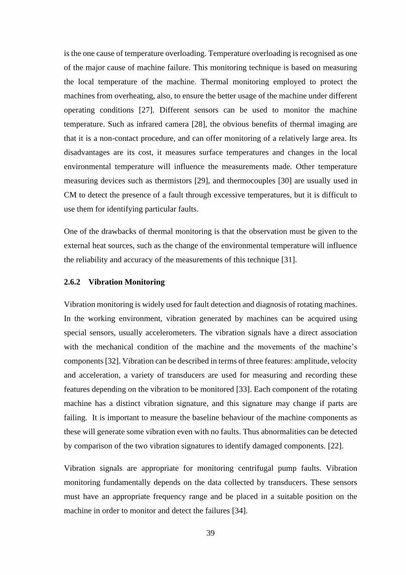
Figure 3-2 Types of centrifugal pumps [62] ..................................................................... 47

Figure 3-3 Cross-section and flow path of a centrifugal pump [68] ............................... 48

Figure 3-4 Radial flow centrifugal pump [71] ................................................................. 48

Figure 3-5 Diagram of axial flow pump [72] ................................................................... 49

Figure 3-6 Diagram of a mixed flow pump [74] .............................................................. 50

Figure 3-7 Main components of a centrifugal pump [75] ................................................ 50

Figure 3-8 Centrifugal pump impeller types: (a) open, (b) semi-open, (c) closed [73] ... 51

Figure 3-9 Construction of mechanical seal [88] ............................................................ 53

Figure 3-10 Ball bearing components [89] ...................................................................... 54

Figure 3-11 Performance characteristics of a centrifugal pump [95]. ............................ 56

Figure 3-12 Three-phase induction motor construction [117] ........................................ 60

Figure 4-1 Time domain current signal for flow rate 350 l/min ...................................... 69

Figure 4-2 Envelope Analysis Method [150]. .................................................................. 74

Figure 4-3 Flowchart of the EMD algorithm [156]. ........................................................ 76

Figure 4-4 Illustration of the EMD method [157]. ........................................................... 78

Figure 4-5 Illustration of standard ITD method, decomposing x(t) into Lt and Ht [167] 80

Figure 4-6 Flow chart of ITD algorithm .......................................................................... 81

18

Figure 5-1 The supervised learning framework [182] ..................................................... 87

Figure 5-2 A hyperplane separating and classifying two classes (a) small margin and (b)

large margin [190] ........................................................................................................... 89

Figure 5-3 The One-Against-All approach of multi-class SVM [196]. ............................ 93

Figure 5-4 The One-Against-One approach of multi-class SVM [196]. .......................... 93

Figure 5-5 SVM with a Directed Acyclic Graph for a multi-classification problem [198].

.......................................................................................................................................... 94

Figure 6-1 The test-rig facility ......................................................................................... 99

Figure 6-2 The centrifugal pump used in this work (Pedrollo Model F32/200) ............ 100

Figure 6-3 A schematic diagram of the test facility. ...................................................... 101

Figure 6-4 The current measurement unit ...................................................................... 102

Figure 6-5 The output of the HTC .................................................................................. 103

Figure 6-6 Schematic of GEMS RFO electronic flow sensor ......................................... 103

Figure 6-7 Electronic flow sensor in the pipeline .......................................................... 104

Figure 6-8 Raw data from the GEMS RFO flow rate sensor ......................................... 104

Figure 6-9 Pressure transducers installed at the pump inlet and outlet ........................ 106

Figure 6-10 Omron speed controller, external and internal views ................................ 107

Figure 6-11 Mounted Hengstler shaft encoder .............................................................. 108

Figure 6-12 Raw data of Shaft encoder .......................................................................... 108

Figure 6-13 Vibration transducer mounted on the pump ............................................... 109

Figure 6-14 Output signal of the accelerometer ............................................................ 110

Figure 6-15 YE6232B Data Acquisition System (DAS) .................................................. 111

19

Figure 6-16 The performance of the centrifugal pump .................................................. 112

Figure 6-17 (a) Inner race defect (b) Outer race defect ................................................ 114

Figure 6-18 Pump head vs Flow rate for (i) healthy pump (baseline), (ii) pump with inner

race fault and (iii) pump with outer race fault ............................................................... 114

Figure 6-19 Blockage impeller ....................................................................................... 115

Figure 6-20 Pump head vs Flow rate for (i) healthy pump (baseline), and (ii) pump with

outer race fault and impeller blockage ........................................................................... 115

Figure 7-1 Time-domain waveforms for baseline, inner race, outer race and combined

fault (outer race and impeller blockage) under different flow rates .............................. 120

Figure 7-2 Motor current RMS values for a healthy pump, and faulty conditions at

different flow rates .......................................................................................................... 121

Figure 7-3 Kurtosis values for the current signal for four pump conditions under different

flow rates ........................................................................................................................ 122

Figure 7-4 Vibration envelope spectral analysis for baseline and inner-race fault under


Figure 7-5 Vibration envelope spectral analysis for baseline and outer race fault under


Figure 7-6 Current spectrum for baseline and inner race fault at three flow rates ....... 125

Figure 7-7 Current spectrum for baseline and outer race fault at three flow rates ....... 125

Figure 7-8 Current spectrum for baseline and combined fault (outer race and impeller

blockage) for three flow rates ......................................................................................... 126

Figure 7-9 Peak value of fundamental supply frequency for the healthy pump and pump

with seeded faults under different flow rates .................................................................. 126

Figure 7-10 Envelope spectrum of current signal for baseline and inner race fault under


20

Figure 7-11 Envelope Spectrum Analysis of current signal for baseline and outer race

fault under different flow rates ....................................................................................... 128

Figure 8-1 Simulated AM signal and its frequency spectrum: (a) a portion of the raw signal

and (b) frequency spectrum. ........................................................................................... 133

Figure 8-2 EMD results of simulated AM signal............................................................ 133

Figure 8-3 EMD decomposition results of Baseline at 250 l/min .................................. 134

Figure 8-4 EMD decomposition results for the outer race fault at 250 l/min ................ 135

Figure 8-5 EMD decomposition results for the inner race at 250 l/min ........................ 135

Figure 8-6 EMD decomposition results for the combined fault at 250 l/min ................. 136

Figure 8-7 Current spectra of the first 3 IMFs for all cases at.250 l/min ...................... 137

Figure 8-8 Peak values at fs from the current spectrums of IMF1 and IMF2 ............... 138

Figure 8-9 Envelope spectrum of IMF1, IMF2 and IMF3 for all cases at 250 l/min. ... 139

Figure 8-10 Peak value of fs from the envelope spectrum for IMF1 and IMF2 ............ 140

Figure 9-1 ITD decomposition result for the healthy pump at 350 l/min. ...................... 144

Figure 9-2 ITD decomposition results for inner race bearing fault at 350 l/min. ......... 144

Figure 9-3 ITD decomposition results for outer race bearing fault at 350 l/min. ......... 145

Figure 9-4 ITD decomposition results for the combined fault of impeller blockage and

outer race defect, at 350 l/min. ....................................................................................... 145

Figure 9-5 RMS of current signals at different flow rates (a) raw data, (b) first PRC. . 147

Figure 9-6 Figure 9-7 Fault separation based on static and dynamic features of the current

signal............................................................................................................................... 148

Figure 10-1 An adaptive diagnostic approach for a centrifugal pump based on data

analysis and SVM. .......................................................................................................... 152

21

Figure 10-2 Confusion matrix of multi-class SVM based on ITD features .................... 154

Figure 10-3 Multi-class SVM classification results using ITD features ........................ 155

Figure 10-4 Confusion matrix of multi-class SVM based on EMD features .................. 156

Figure 10-5 Multi-class SVM classification results using EMD features ...................... 157

Figure 10-6 SVM Confusion matrix of multi-class SVM based on DWT features ......... 158

Figure 10-7 Multi-class SVM classification results using DWT features ...................... 159

Figure 10-8 SVM Confusion matrix of multi-class SVM based on envelope features .... 160

Figure 10-9 multi-class SVM classification results using envelope features ................. 161

Figure 10-10 Comparison between different feature extraction techniques .................. 162

22

List of Tables

Table 6-1 Specification of the centrifugal pump ............................................................. 100

Table 6-2 Specification of the three-phase HTC unit ..................................................... 102

Table 6-3 Specifications of GEMS RFO flow rate sensor .............................................. 105

Table 6-4 Specifications of the pressure transducer ...................................................... 106

Table 6-5 Speed controller specifications ...................................................................... 107

Table 6-6 Specifications of the shaft encoder ................................................................. 109

Table 6-7 Specifications of the accelerometer ................................................................ 110

Table 6-8 Technical specification of the data acquisition .............................................. 112

Table 6-9 Characteristics of the bearing ........................................................................ 113

Table 10-1 Data set of statistical features (experimental data) ..................................... 153

Table 10-2 Multiclass SVM class names ........................................................................ 153

Table 10-3 Comparison of diagnostic results obtained using the different techniques for

all cases .......................................................................................................................... 161

Table 10-4 Comparison of the current work with the comparable work reported in the

literature ......................................................................................................................... 163

23

List of Abbreviations

MCSA Motor current signature analysis

ESA Electrical signal analysis

MSS Motor supply signals

CM Condition monitoring

ITD Intrinsic time scale decomposition

EMD Empirical mode decomposition

SVM Support vector machine

CBM Condition-based maintenance

ORNL Oak Ridge National Laboratory

FFT Fast Fourier transform

DWT Discrete wavelet transform

WPD Wavelet packet decomposing

CWT Continuous wavelet transformation

SWT Stationary wavelet transform

HHT Hilbert-Huang transform

MSB Modulation signal bispectrum

BEP Best efficiency point

NPSH Net positive suction head

NPSHr Net positive suction head required

NPSHa Net positive suction head available

RMS Root mean square

EMF Electromagnetic force

CT Current transducer

CF Crest factor

SC Spectral centroid

SS Spectral spread

SF Spectral Flux

STFT Short time Fourier transform

WT Wavelet transform

IMF Intrinsic mode function

24

ICA Independent component analysis

ANN Artificial neural network

PRC Proper rotation component

RVM Relevant vector machine

ML Maximum likelihood

OAA One-against-the all

OAO One-against-one

DAG Directed acyclic graph

DAS Data acquisition system

IAS Instantaneous angular speed

AM Amplitude-modulating

BL Baseline

RBF Radial basis function

K-CV K-fold cross-validation

25

List of Nomenclatures

Symbol Description

vH

Velocity Head

sH

Static head

fH

Friction head

Q

Pump capacity

fE

Efficiency of pump

fE

Efficiency of pump

wP

Hydraulic power

sP

shaft power

ah

Head suction

vph

Vapour pressure

fh

Friction losses

Linkage flux

sf Fundamental frequency

T Torque

J Motor inertia

Angular displacement

P Number of pole pairs

( )X t Time domain signal

( )t The wavelet function

26

Introduction

The chapter provides a brief introduction to the research presented in this thesis. It

outlines the study background, research applications, and provides the motivation for this

study. Also, the main aim and objectives are presented. Finally, the contents of the thesis

chapters are listed.

27

1.1 Background

Condition monitoring (CM) is a vital requirement for evaluating the condition of rotating

machines. It has been used for identifying faults, preserving machine efficiency, reducing

unexpected damage, and lowering maintenance cost [1]. CM plays a significant role by

monitoring parameters such as vibration and current amplitudes that indicate changes in

the mechanical and/or the electrical condition of the machine while in operation. Routine

preventive maintenance can also protect against catastrophic failure, provided the time

intervals between inspections is short enough. In industry, these periods are often the result

of experience and advice from the manufacturer’s of the machines. By monitoring physical

parameters that enable the condition of the machine to be determined, developing faults

can be identified and the remaining working life can be predicted [2, 3]. It is now generally

accepted that CM should be implemented as the best way for reducing downtime and

maintenance costs, preventing machine failure and enhancing operational uptime [4, 5].

CM methods can be classified into two types: intrusive monitoring techniques, such as

vibration monitoring, where installation of sensors on the machine is necessary to acquire

the necessary data. The other type is non-intrusive monitoring, which includes electric

signal monitoring, and which it does not require sensors to be installed on the machine [6].

While each method has its limitations, electric signal monitoring is a desirable technique

for those industrial applications where external sensors are difficult to install because of,

for example, insufficient space or harsh environmental conditions. The latter has the

advantage of relatively easy installation and can begin monitoring the machine’s condition

without any interruption to its operation [7]. Therefore, CM based on electrical signal

analysis should be examined for developing and applying advanced signal analysis

techniques to detect machine defects. While it is essential to avoid catastrophic failures by

using robust CM techniques, detection of faults at an early stage would be highly

advantageous but will require highly accurate diagnostic techniques [8, 9].

CM normally includes three main steps: acquiring data, processing the data and

interpretation of the data [10]. An essential part of CM is to reliably acquire accurate data

about the machine's condition to determine whether the operating condition is normal or

not. Also, essential is the use of suitable techniques for analysing the acquired data and

capturing useful information for determining the machine’s condition and identifying any

28

developing fault. This information should be sufficient for diagnostic and prediction

purposes. This will assist the maintenance team in determining appropriate action.

Electrical signal analysis (ESA) is a powerful CM method used to detect and diagnose

damage in machine systems. However, the current signal is invariably contaminated by a

variety of noise, most of which will be produced by non-linear processes. Thus, it is usually

difficult to capture accurately diagnostic features with conventional data analysis methods.

This research focuses on investigating current data obtained from an electrical control

system and investigates the motor signals based on data-driven techniques to enhance the

CM of a rotating machine, a centrifugal pump.

1.2 Research Application and Motivation

Because of their simplicity of design and flexibility in use, centrifugal pumps are widely

used in numerous manufacturing processes and applications, for example, agricultural

irrigation, chemical plants, oil and gas industry [11, 12]. The components of a centrifugal

pump may fail during operation due to excessive stress on, and reduced strength of, its

component parts. These failures occur in ways that affect the efficiency of the pump, and

may interrupt the manufacturing process, causing cessation of production [13].

It would be very useful to have detection and precise diagnosis, of faults developing in

centrifugal pumps. This would help maximise production by allowing efficient long-term

maintenance scheduling and avoidance of unexpected shutdowns. A CM system that is

reliable and low-cost is highly desirable, and an exciting area of research is to improve the

long-term performance of centrifugal pumps.

However, the monitoring of centrifugal pumps is still challenging because of the limited

access to many pumps and the consequent difficulty in installing or accessing in-situ

sensors such as accelerometers. Such sites would include the very important nuclear and

off-shore oil and gas industries [14]. It would be extremely useful for these, and many

other, industries to have available enhanced CM methods, including diagnostic techniques

for analysing the data acquired from a pump’s electrical control system, where the current

signal is easy to obtain at any appropriate location without any interruption of the machine.

Hence, there has developed a trend for employing techniques that require less equipment

and non-intrusive sensors for collecting CM data.

29

Using Motor Current Signal Analysis (MCSA) for monitoring the condition of the pump

is thus a potentially powerful and useful tool [14]. It has been shown to be a reliable and

beneficial method for monitoring rotating machinery [15]. Thus, monitoring the condition

of a centrifugal pump based on the current signature of the driving motor is considered an

interesting topic for research: to demonstrate that it is possible to thoroughly investigate

pump characteristics using data analysis techniques based MCSA.

However, the motor current is subjected to noise interference which is a function of the

given operating conditions, and will invariably be a complicated non-linear, and non-

stationary process. Therefore, advanced data analysis techniques are necessary for

detection of a fault before a complete breakdown of the pump operation.

Machine Learning (ML) paradigms and data-driven methods are adopted in this research

to analyse non-stationary current signals for different pump conditions. With these

methods, such as empirical mode decomposition (EMD) and intrinsic time-scale

decomposition (ITD), the decomposed signals provide a baseline which is determined

from the signals themselves, rather than finding the similarity to specified basis functions,

such as in wavelet transformations. The diagnostic features can be seen, and the underlying

trends on the signals can be captured, providing meaningful information for more effective

and accurate fault identification. However, the author believes that no reports were found

in the literature where ITD was used for analysing pump motor current signals. It is this

specific application that is one of the novel features of this project. Later classification

method based on the support vector machine (SVM) algorithm will be used for

distinguishing centrifugal pump faults (simulated faults).

Thus, the motivation for this research is to produce a robust method for extracting useful

information that will accurately identify diagnostic features using data-driven techniques

in a platform and overcome the serious limitations of conventional data analysis techniques

[16]. In particular, the platform will be used to investigate modulating frequencies

contained in the current signals to accomplish high-performance diagnostics of rotating

machines.

30

1.3 The Aim and Objectives of the Research

The aim of this research project is to produce a platform using advanced ML paradigms

capable of analysing the motor current signals of centrifugal pumps to detect developing

faults and produce an accurate diagnosis.

The specific objectives of this thesis can be summarized as follows.

Objective 1. To review CM methods and maintenance strategies and explain the most

common techniques used for fault detection of centrifugal pumps.

Objective 2. To refine the existing test facility and use it for monitoring the condition of

a centrifugal pump with different simulated pump faults under various flow rates.

Objective 3. To examine the ability of motor current data obtained from the electrical

control system for detecting various mechanical faults of the pump by examining the

current signature using various signal process techniques.

Objective 4. To explore the current signal under different operating conditions using

conventional data analysis methods to identify and obtain the most critical fault

defining feature, that will be used for comparison with those obtained from the data-

driven techniques.

Objective 5. To explore and apply data-driven techniques for extraction of the weak

nonlinear characteristics of the current signals that are affected by, for example,

fluctuations in pump operating pressures and flow rate, and various electromagnetic

noises interfering with the measured signals.

Objective 6. To examine supervised machine learning techniques such as SVM, for

enhancement of CM performances based on the electrical data from the motor.

Objective 7. To investigate and evaluate the use of ITD combined with SVM

classification algorithm to detect and diagnose the seeded faults. Also, to compare the

results of the proposed method with those adopted using a combination of the SVM

algorithm with EMD, with DWT and with envelope analysis. The results will also be

compared with those of other researchers in this area.

Objective 8. To provide meaningful recommendations for future research in this

particular subject.

31

1.4 Thesis Organisation

The thesis is divided into eleven chapters, including the current chapter that contains

background, research application and motivation, and the research aim and objectives. An

outline of each subsequent chapter is presented below:

Chapter 2 starts by introducing CM, and the importance of a maintenance strategy for

manufacturing processes, also it provides a brief introduction to commonly used CM

techniques for detecting and diagnosing of rotating machinery faults. Finally, the chapter

addresses the motor current signal analysis, which is the main subject of this research.

Chapter 3 describes the common configurations of the centrifugal pump and its

mechanical construction. It also explains the driver induction motor, following by the

pump failure modes. Finally, the impacts of centrifugal pump operation under different

conditions on the current signature of the electrical motor are presented.

Chapter 4 presents a literature overview of data analyses methods for extracting

monitoring information. It demonstrates the advantages of the data analyses based on data-

driven methods for detection and identification of machine faults. This chapter mainly

focuses on the MCSA method relevant to detecting and diagnosing different centrifugal

pump faults.

Chapter 5 presents an overview of machine learning paradigms used for machine fault

diagnosis. It explains the supervised learning framework. Details of the SVM technique

and feature extraction method are provided to classify the centrifugal pump faults.

Chapter 6 describes the experimental facilities used in this study. It explains the

construction of the centrifugal pump test rig, describes all components and control systems

that are used to carry out the investigation, with the motor current measurement system.

Finally, simulated faults are described and illustrated, and the experimental procedure is

presented.

Chapter 7 presents the investigation of the centrifugal pump fault detection under

different operating conditions based on analysing the motor current signal with

conventional signal analysis methods. Time domain and frequency domain techniques are

used to examine the changes in the current signature related to the pump operation; the

32

waveform representation shows the modulation effect on the current signal. Finally,

common statistical parameters are presented.

Chapter 8 shows the detection of the impeller and bearing faults based on the Empirical

Mode Decomposition (EMD) technique for extracting features of the current motor

signature. The envelope technique is also used for demodulating the current signal and

detecting abnormal conditions in the centrifugal pump.

Chapter 9 investigates a data-driven technique for analysing and decomposing the motor

current signal, and its application for detecting the centrifugal pump faults. Intrinsic Time

Scale Decomposition (ITD) is used to examine the condition of the centrifugal pump. Root

mean square of ITD is shown to have the capability for detecting and characterizing the

pump fault.

Chapter 10 investigates the efficiency of using a machine learning method for classifying

the faults in the centrifugal pump based on current signals. SVM classifiers are constructed

using statistical parameters. In addition, this chapter introduces the diagnostic approach

based on the proposed method (ITD and SVM), a comparison of effective features for

diagnostic faults is carried out using other methods (Envelope, EMD and DWT) in order

to evaluate the performance of the proposed method.

Chapter 11 concludes the thesis, it presents the conclusions, reviews the achievements

against the objectives, and describes contributions to knowledge and novel aspects; finally,

the chapter proposes some topics for future work

The summaries of the general structure of the research work and the scheme developed

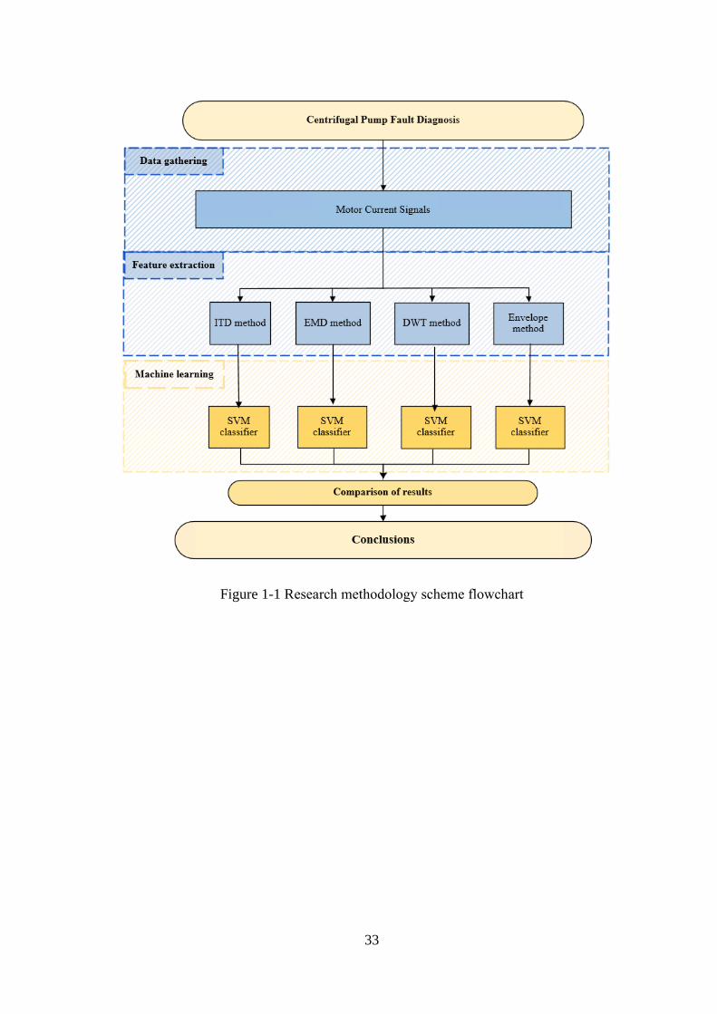
showed in Figure 1-1.

The flowchart explains the main steps for achieving the objectives of this study. The

process starts with the current signals being gathered from the centrifugal pump test rig.

In the second stage, the current signals are analysed to extract statistical features by using

the proposed method ITD and by other signal processing techniques (Envelope, ITD and

DWT), then a machine learning algorithm (SVM) is employed for generating the

classifiers based on these features, and used for diagnosing the particular centrifugal pump

faults.

33

Figure 1-1 Research methodology scheme flowchart

34

Condition Monitoring

This chapter begins by presenting basic Condition Monitoring (CM) techniques. It

explains the main CM methods and essential maintenance strategies. It then describes

various CM techniques used for the detection of common machinery faults, which includes

critical comments on each of the techniques in order to gain sufficient understanding of

them and subsequently identify the potential of applying emerging signal processing

techniques for improving the performance of CM systems.

35

2.1 Introduction

Rotating machines are extensively employed in commercial systems and industrial plant.

They require regular monitoring to assess their condition to take an appropriate decision

for maintenance work. Early stage faults, if undetected may grow to adversely affect the

efficiency of the plant or cause a catastrophic failure. Monitoring of downstream

mechanical systems can provide accurate and prompt fault detection and adequate

information for the task of decision-making. Therefore, fault detection and isolation of

rotating machines such as gearbox boxes, wind turbines, and centrifugal pumps are

essential to provide stability of performance and to minimise operating costs.

2.2 Condition Monitoring Overview

CM is the procedure for determining the condition of the rotating machine by monitoring

associated parameters with the machine working; it is used to decrease the maintenance

cost, ensure machine efficiency and even extend the working life of the machine. It has

been widely used to examine and develop techniques for early detection of initial faults

[17]. CM is an essential tool for fault detection and diagnosis, it provides continuous

assessment of machines, provides an early warning of the expected failures and makes it

possible to reschedule future maintenance. It reduces downtime and ensures the reliability

of scheduled maintenance [18]. There are many goals of using CM in industry, such as

[19]:

• Improve machine reliability and availability.

• Decrease maintenance expenses.

• Enhance safety performance.

• Predict equipment failure.

• Increase the accuracy of fault prognosis.

• Promote the reliability of machine components.

• Enhance equipment performance.

• Eliminate unscheduled downtime.

CM has attracted attention in many branches of research, especially determining the most

appropriate monitoring technique for fault detection and identification in specific

appliances such as pumps.

36

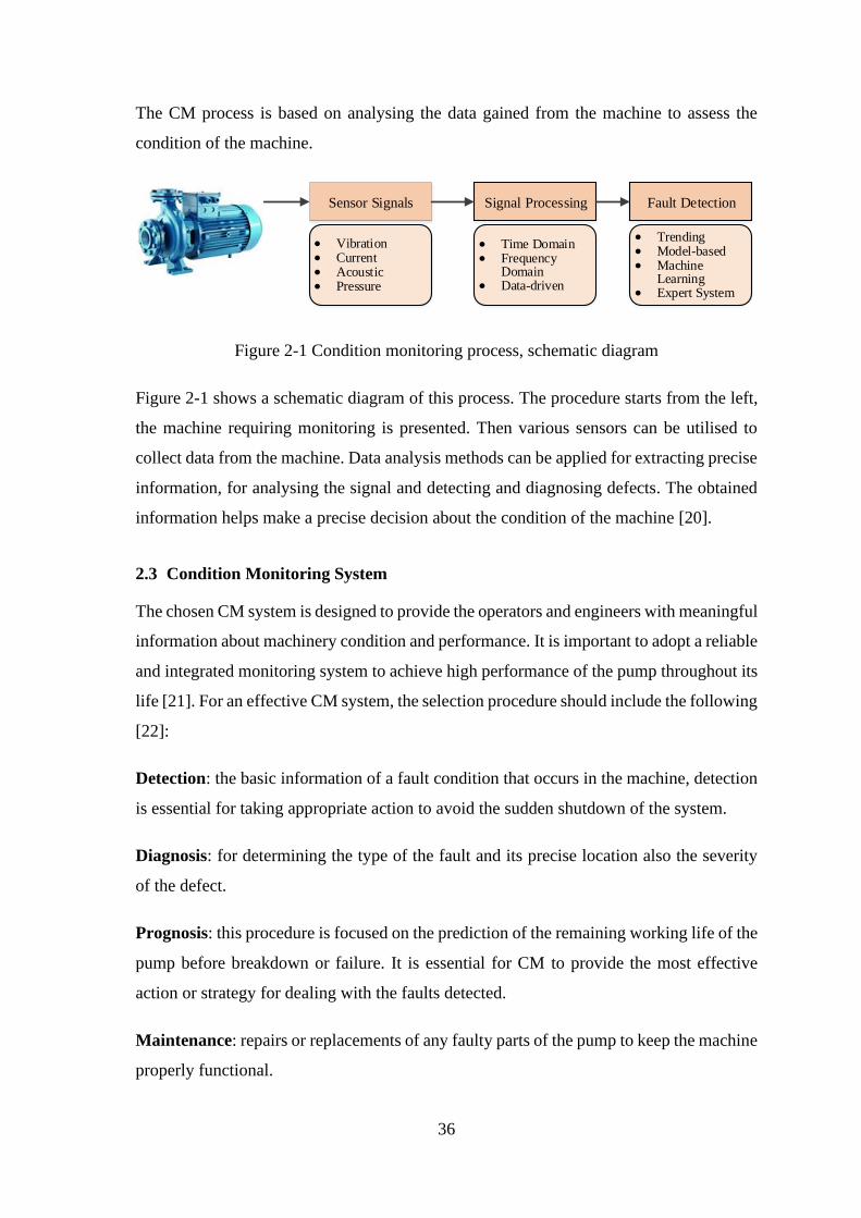
The CM process is based on analysing the data gained from the machine to assess the

condition of the machine.

Sensor Signals Signal Processing Fault Detection

• Vibration• Current• Acoustic• Pressure

• Time Domain • Frequency

Domain • Data-driven

• Trending• Model-based• Machine

Learning• Expert System

Figure 2-1 Condition monitoring process, schematic diagram

Figure 2-1 shows a schematic diagram of this process. The procedure starts from the left,

the machine requiring monitoring is presented. Then various sensors can be utilised to

collect data from the machine. Data analysis methods can be applied for extracting precise

information, for analysing the signal and detecting and diagnosing defects. The obtained

information helps make a precise decision about the condition of the machine [20].

2.3 Condition Monitoring System

The chosen CM system is designed to provide the operators and engineers with meaningful

information about machinery condition and performance. It is important to adopt a reliable

and integrated monitoring system to achieve high performance of the pump throughout its

life [21]. For an effective CM system, the selection procedure should include the following

[22]:

Detection: the basic information of a fault condition that occurs in the machine, detection

is essential for taking appropriate action to avoid the sudden shutdown of the system.

Diagnosis: for determining the type of the fault and its precise location also the severity

of the defect.

Prognosis: this procedure is focused on the prediction of the remaining working life of the

pump before breakdown or failure. It is essential for CM to provide the most effective

action or strategy for dealing with the faults detected.

Maintenance: repairs or replacements of any faulty parts of the pump to keep the machine

properly functional.

37

2.4 Maintenance Strategies

There are three types of maintenance strategies, one is based on breakdown maintenance,

and the other types are based on predicting and preventive maintenance, Selection of the

most appropriate maintenance approach depends on the machine to be assessed and the

experience of the maintenance team. Run-to-breakdown allows the machinery to run-to-

failure while preventive and predictive maintenance represents early remedial actions to

avoid equipment breakdowns, the main purposes of maintenance strategy are [23]:

•To develop and preserve productivity.

•To ensure a high quality of products.

•To increase the lifetime of the machine.

•To decrease the number of repairs and replacement procedures.

2.4.1 Run to Break Maintenance

This type of maintenance is considered as the traditional maintenance method, the machine

is operated until breakdown happens. This method allows the machine to keep operating

until shutdown, but failure can be catastrophic and result in severe damage. In this strategy,

the maintenance is performed only after the machine breaks down. Run to breakdown is

still used in some industries where production is not, or only a little, affected by losing one

machine for a short time. These industries tend to have a high number of small machines

in operation [2].

2.4.2 Preventive Maintenance

This strategy is based on a certain period of time between scheduled maintenance visits; it

is more appropriate where the time to failure can be sensibly predicted. It aims to extend

the working life of the machine and prevent breakdowns. It involves activities such as

monitoring without intervention. In this strategy, a predetermined monitoring routine is

performed on a particular machine to evaluate its operation and system health to decide

which equipment or parts need more investigation or even replacement. During this latter

process, the system may require a shutdown, a good plan allows scheduling of the best

time for system-shutdown for repairing and maintaining the machines [24].

38

2.4.3 Predictive Maintenance

This approach is based on precise measurements in real-time operation. It requires a

reliable CM technique; the maintenance events can be scheduled in advance depending on

the particular criteria used for making any necessary predictions. It gives the management

team a time limit for purchasing necessary parts for repair rather than having a big

inventory of replacement parts. Predictive maintenance can extend the period between

preventive maintenance actions, and as it detects the faults in an early time, predictive

maintenance prevents catastrophic failures [25].

2.5 Condition Based Maintenance

Condition based maintenance (CBM) is a technique that monitors the machine and

recommends maintenance decisions using the meaningful information obtained from the

machine being monitored. Generally, CBM involves three essential stages: data gathering,

data analysis, and maintenance decision making. CBM is capable of providing a robust

technique for reducing maintenance costs and ensuring the efficacy of the machine. It is

employed to avoid unnecessary maintenance tasks by helping to reduce the number of

unessential scheduled preventive activities, hence, reducing the maintenance cost of the

machine [10].

2.6 Condition Monitoring Techniques

There are many techniques used for monitoring rotating machinery CM is processes to

monitor parameters or condition such as vibration, temperature, pressure and current signal

in the system, that involves observing the components of the machine to detect changes in

operation that can be indicative of developing failures [26]. Selecting an appropriate

technique depends on its capabilities and limitations for detecting early changes in the

parameters and trends. CM is used as a part of the condition monitoring system to prevent

unplanned breakdown and reduces the maintenance cost. The following methods are

generally utilised for detecting and diagnosing machine faults:

2.6.1 Thermal Monitoring

It is one of common indicator of the machine condition. Worn machinery parts and

damaged material components can lead to abnormal temperature distribution. The friction

39

is the one cause of temperature overloading. Temperature overloading is recognised as one

of the major cause of machine failure. This monitoring technique is based on measuring

the local temperature of the machine. Thermal monitoring employed to protect the

machines from overheating, also, to ensure the better usage of the machine under different

operating conditions [27]. Different sensors can be used to monitor the machine

temperature. Such as infrared camera [28], the obvious benefits of thermal imaging are

that it is a non-contact procedure, and can offer monitoring of a relatively large area. Its

disadvantages are its cost, it measures surface temperatures and changes in the local

environmental temperature will influence the measurements made. Other temperature

measuring devices such as thermistors [29], and thermocouples [30] are usually used in

CM to detect the presence of a fault through excessive temperatures, but it is difficult to

use them for identifying particular faults.

One of the drawbacks of thermal monitoring is that the observation must be given to the

external heat sources, such as the change of the environmental temperature will influence

the reliability and accuracy of the measurements of this technique [31].

2.6.2 Vibration Monitoring

Vibration monitoring is widely used for fault detection and diagnosis of rotating machines.

In the working environment, vibration generated by machines can be acquired using

special sensors, usually accelerometers. The vibration signals have a direct association

with the mechanical condition of the machine and the movements of the machine’s

components [32]. Vibration can be described in terms of three features: amplitude, velocity

and acceleration, a variety of transducers are used for measuring and recording these

features depending on the vibration to be monitored [33]. Each component of the rotating

machine has a distinct vibration signature, and this signature may change if parts are

failing. It is important to measure the baseline behaviour of the machine components as

these will generate some vibration even with no faults. Thus abnormalities can be detected

by comparison of the two vibration signatures to identify damaged components. [22].

Vibration signals are appropriate for monitoring centrifugal pump faults. Vibration

monitoring fundamentally depends on the data collected by transducers. These sensors

must have an appropriate frequency range and be placed in a suitable position on the

machine in order to monitor and detect the failures [34].

https://www.sciencedirect.com/topics/engineering/thermocouples

40

The main drawback of vibration monitoring is that the vibration transducers are not always

easy to install, such as on inaccessible machines [35].

2.6.3 Acoustic Emission Monitoring

The acoustic emission (AE) technique works in a comparable manner to the vibration

technique. Acoustic emission is a non-directional method, so it can use one sensor for

measuring the signal compared with the vibration technique that may require up to three

axes for gathering the necessary data. AE is a sensitive technique that can give good results

when used for CM of machines and detection of faults. AE detects high-frequency signals,

typically in the range 20 kHz to 1 MHz [36].

AE is defined as high-frequency stress waves generated by the interaction between two

surfaces in relative movement [37] and any change of acoustic signature generated by the

rotating machine may indicate damage of one or more machine parts [38].

AE is a non-intrusive method for the CM of the rotary machine, and can offer useful

information about the machine’s condition [39].

Baydar and Ball [40] have applied the wavelet transform on the acoustic signal for

detection of faults in a gearbox, and claim that results achieved by AE analysis are more

effective than those obtained by vibration analysis. Alfayez and Mba [41] have

investigated the usage of AE for detecting incipient cavitation in a centrifugal pump. Their

analysis showed that there is an increase in the AE level when cavitation first appears in

the operation of the pump. AE has received very little attention compared to vibration

monitoring because the acquired signals are more difficult to process, interpret and classify

[38].

2.6.4 Electrical Signature Analysis (Current Monitoring)

MCSA is a monitoring technique developed at the Oak Ridge National Laboratory [42].

As an appropriate method for CM in a varied range of applications. MCSA is based on the

induction motor driving a mechanical load being regarded as a permanently available

transducer sensing changes in the mechanical load, and converting them into variations in

the induced current generated in the motor windings. These changes in motor current are

carried in the electrical cables connecting the motor and can be extracted at any appropriate

41

location without any interruption of the machine. Only a single transducer is required [43].

It is a non-intrusive method [44], where faults in downstream equipment driven by

induction motors can be indirectly detected by monitoring the motor current signal [45].

MCSA is based on stator current monitoring, which contains frequency components

related to numerous defects that occur in the machine. Any defect in the rotating machine

operated by an induction motor like a gearbox or pump will produce a change in the load

torque on the rotor of the motor. Thus a magnetic force will be induced in the stator coils.

Consequently, the current signal will be modulated and sidebands around the supply

frequency will be generated and can be detected [45]. MCSA is a robust technique for

determining defects in mechanical systems that are otherwise inaccessible for condition

monitoring by vibration analysis such as submersible pumps, where the current data of the

pump are just required to access the supply lines carrying the current [46]. Therefore,

current monitoring can be applied without any extra devices. It is an effective method for

fault detection of the electrical and mechanical equipment.

MCSA can be implemented economically and effectively to analyse and evaluate the

electrical and mechanical condition of a machine, for avoiding catastrophic failures and

saving on maintenance cost [47].

It has been widely used in monitoring various rotating machines, including gearboxes,

centrifugal pumps, and reciprocating compressors. Luo, et al., [48] employed a sensorless

monitoring method based on MCSA using FFT analysis for identifying the occurrence of

cavitation in a centrifugal pump. Results showed that characteristics of the current

spectrum such as the harmonics and vane pass frequency components exhibited

characteristics related to the cavitation stage, these changed as the cavitation progressed.

Singh, et al., [49] have used MCSA for bearing fault detection in a mechanical system,

they explained that the defects in a bearing mounted in a bearing house can be detected

through the change in the magnitude of the motor current harmonics, and sidebands appear

around the shaft frequency. A continuous wavelet transform (CWT) was applied to detect

an outer race fault.

Popaleny, et al., [50] have examined the effect of mechanical and electrical defects in the

current of electrical submersible pumps and their reflection in the dynamic current

42

spectrum. Different defects such as broken rotor bars, mass unbalance and process issues

such as cavitation were investigated using MCSA and power spectral density plots. Results

showed that the MSCA was able to identify the defects that occurred.

Martin, et al., [51] have investigated the influence of broken rotor bar faults in an induction

motor. Traditional MCSA was used for detecting these faults. For more efficient

monitoring of the system, MSCA can be combined with other techniques. For example,

Magdaleno, et al., [52], have proposed method based on MCSA with a neural network

algorithm for detecting broken rotor bar faults.

However, the classical MCSA based method has certain drawbacks. When the pump is

operated under continuous load variations or in the case of ‘pulsating load torque’, its

speed is not constant, which might be misinterpreted in the Fourier spectrum of the currents

and can lead to an incorrect diagnosis of failure [53]. Niu et al. [54] applied the discrete

wavelet transform (DWT) to a transient stator current signal for diagnosing faults in an

induction motor. For the classification task, their study used a decision-level fusion model.

Inaki, et al., [55] used MCSA for assessing the condition of a gearbox operating under

different speeds. The acquired current data were analysed by both DWT and dual-level

time asynchronous techniques. This approach allowed the differentiation of healthy

gearboxes from faulty cases. MSCA with wavelet packet transform (WPT) was applied

for detection of outer bearing fault [56]. Kar and Mohanty studied MCSA for monitoring

transmission gearboxes and investigated two defects; one tooth broken, and two teeth

broken. The study compared the performance of DWT relative to CWT and found that

gearbox defects could be identified more effectively using DWT for analysing the current

signals, than CWT [57].

Kompella, et al., [58] applied the MCSA to detect bearing faults utilising frequency

spectral subtraction based on different wavelet transforms such as DWT and the stationary

wavelet transform (SWT). These techniques were implemented and compared based on a

number of indexing fault parameters. The results showed that the proposed method was

suitable and effective for differentiating the bearing faults.

Nevertheless, analysing signals by wavelet transforms is not easy, as choosing predefined

mother wavelet is itself difficult. Meaning some characteristics of important frequencies

43

may not be captured by the selected wavelet base, which could lead to loss of useful

information for diagnosing faults.

Sun, et al., [59] investigated centrifugal pump operation under different conditions. Both

current and vibration data were collected under normal and cavitation conditions. Then the

signals were interrogated using the Hilbert-Huang Transform (HHT). The results showed

that an unstable flow rate due to cavitation in the pump would produce an energy variation,

and the time-frequency characteristics of the signal, such as RMS, extracted from the

results of the HHT process can be used to detect pump operating conditions. Amirat et al.,

[60] have proposed a diagnostic method based on ensemble EMD of the motor phase

current for bearing faults detection. Three defects were investigated: cage defect, ball

defect, and inner race defect. The closest intrinsic mode function (IMF) based on a Pearson

correlation was removed from the original signal, after that standard deviation as fault

criterion was calculated and used to specify the condition of the induction motor, where

the faulty conditions have higher values than the healthy case. However, this study did not

investigate how to distinguish between different fault cases.

Tian, et al., [7] utilized a modulation signal bispectrum (MSB) technique for extracting

nonlinear characteristics of the current signal acquired from the motor driving a centrifugal

pump system under different impeller faults. Results showed that this method was capable

of effectively detecting impeller faults. MSB was found to be capable of capturing the

sidebands around the vane pass frequency from the current spectrum.

MCSA is a powerful technique for determining faults in mechanical systems where the

machine is inaccessible, or more traditional sensors are difficult to install or access [45].

However, MSCA requires more investigation to assess how to extract more meaningful

information, which is usually hidden by noise, from the acquired signal. An advanced

signal processing technique is necessary for analysing nonstationary and nonlinear signals,

to extract and reveal features from the acquired current signal. Here the study focuses on

using the data-driven techniques with machine learning as these can offer more effective

and accurate for fault detection and diagnosis.

44

2.7 Key Findings

The basic concepts and scope of CM technologies have been presented, which was

explained in association with the main elements of a maintenance strategy. The most

important CM methods such as vibration, acoustics and thermal imaging have been

described in this literature overview. Although these methods are of proven worth, they

generally have one or more deficiencies in their use, e.g., inconvenient setup, expensive

hardware and complex computations.

Moreover, the literature review demonstrated that MCSA can provide a robust diagnostic

tool for CM, which is safe and efficient and needs less hardware investment. These key

merits of MCSA provide the essential bases for developing more cost-effective CM for

pump systems.

However, more investigation is desirable in order to improve the capabilities of MCSA in

terms of signal noise reduction and enhanced monitoring of weak signal components. It is

proposed to do this by utilizing data analysis techniques based on ML approaches, to

capture the most effective features for enhanced CM of rotating machines. The study will

focus on the detection and diagnosis of faults seeded into a centrifugal pump. The principal

components of such pumps, their types and common failures will be described in the next

chapter.

45

Fundamentals of Centrifugal Pump, Types

and Common Failures

This chapter presents an overview of centrifugal pumps. It explains the construction of the

centrifugal pump and the pump’s performances characteristics in detail. Then, an

overview of the most common failure modes in centrifugal pumps is given with a critical

analysis of their causes and effects. Finally, the motor current signals under pump defects

are presented at the end of this chapter with analysis and explanation of the interactions

between torque load and motor torque.

46

3.1 Introduction

The main task of any pump is to transfer fluid or gas from one point to another. It is a

mechanical device that can be used to move fluid from low-pressure to higher pressure

areas using a rotating impeller to accelerate the liquid by converting electrical energy into

kinetic energy of the fluid [61]. In general, pumps are categorized in terms of the

fundamental operation of the pump; positive displacement pumps and kinetic pumps, as

shown in Figure 3-1.

Figure 3-1 Types of pumps [62]

Positive displacement pumps move a fixed amount of fluid during each discharge stroke.

They have a fixed displacement volume, and the flow rates directly correspond to their

speed. They are typically used for highly viscous fluids under high pressure and low flow

operation. Reciprocating pumps such as a piston are common types of the positive

displacement pump, where the fluid is delivered as a pulsing flow [63].

The second category of pumps is kinetic pumps, where pumping the fluid is achieved by

imparting velocity to the fluid passing through the pump, and subsequently, converting the

velocity into pressure. Centrifugal pump is popular and commonly used for the transfer of

fluids. Figure 3-2 presents the types of centrifugal pumps [64].

47

Figure 3-2 Types of centrifugal pumps [62]

In this research, only the centrifugal pump is considered as it widely used in industry,

offers high capability, a wide range of capacity and is simple and safe to operate [65].

3.2 Basic Concept of Centrifugal Pump

A centrifugal pump is a type of a roto-dynamic pump that is extensively used in

manufacturing, agriculture, petroleum, and chemical industries. Typically, it is used for

systems requiring larger volume flow rates. It is used to transport liquid via a rotating

impeller at high speed [66]. The main purpose of centrifugal pumps is to transfer fluids by

lifting a specific volume flow to a specific required level. The transfer operation of the

pump is based on well understood hydrodynamic processes [67].

A centrifugal pump operates as follows: the rotation of the impeller moves the liquid

outwards, generating a low pressure region at its centre which “draws in” fluid at the pump

inlet. The kinetic energy of rotation of the impeller is transformed into pressure by the

relative movement between the impeller and volute. The fluid pressure is further increased

as the fluid passes through the expansion area. Finally, the high-pressure fluid is

discharged via the discharge nozzle. Figure 3-3 depicts a cross-section of a centrifugal

pump and shows the motion of the fluid [68].

48

Figure 3-3 Cross-section and flow path of a centrifugal pump [68]

3.3 Classification of Centrifugal Pump

Centrifugal pumps can be categorized based on the pattern of the fluid movement through

the pump, the fluid discharge direction, and the point to which the liquid needs to be

moved. In general, there are three types of centrifugal pumps, which are introduced below.

3.3.1 Radial Flow Centrifugal Pump

In a radial flow pump, the direction of the flow is radial, at right angles to the axis of

rotation. The impeller in this type has a large outlet diameter compared to the inlet

diameter. The liquid enters at the centre of the casing and then passes through the impeller,

and is subsequently moved outwards, gaining angular velocity from the rotating shaft. The

blades of radial flow pumps are longer than those of mixed flow pumps [69]. Figure 3-4

shows a typical radial flow centrifugal pump. Radial flow pumps have higher power due

to a large amount of fluid flowing inside the impeller. Furthermore, radial flow pumps

provide higher head pressure compared with the other pumps, but the flow capacity is

smaller [70].

Figure 3-4 Radial flow centrifugal pump [71]

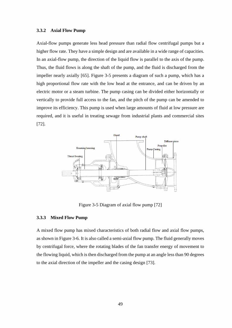
49

3.3.2 Axial Flow Pump

Axial-flow pumps generate less head pressure than radial flow centrifugal pumps but a

higher flow rate. They have a simple design and are available in a wide range of capacities.

In an axial-flow pump, the direction of the liquid flow is parallel to the axis of the pump.

Thus, the fluid flows is along the shaft of the pump, and the fluid is discharged from the

impeller nearly axially [65]. Figure 3-5 presents a diagram of such a pump, which has a

high proportional flow rate with the low head at the entrance, and can be driven by an

electric motor or a steam turbine. The pump casing can be divided either horizontally or

vertically to provide full access to the fan, and the pitch of the pump can be amended to

improve its efficiency. This pump is used when large amounts of fluid at low pressure are

required, and it is useful in treating sewage from industrial plants and commercial sites

[72].

Figure 3-5 Diagram of axial flow pump [72]

3.3.3 Mixed Flow Pump

A mixed flow pump has mixed characteristics of both radial flow and axial flow pumps,

as shown in Figure 3-6. It is also called a semi-axial flow pump. The fluid generally moves

by centrifugal force, where the rotating blades of the fan transfer energy of movement to

the flowing liquid, which is then discharged from the pump at an angle less than 90 degrees

to the axial direction of the impeller and the casing design [73].

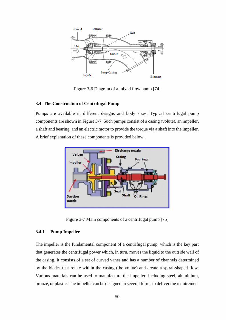
50

Figure 3-6 Diagram of a mixed flow pump [74]

3.4 The Construction of Centrifugal Pump

Pumps are available in different designs and body sizes. Typical centrifugal pump

components are shown in Figure 3-7. Such pumps consist of a casing (volute), an impeller,

a shaft and bearing, and an electric motor to provide the torque via a shaft into the impeller.

A brief explanation of these components is provided below.

Figure 3-7 Main components of a centrifugal pump [75]

3.4.1 Pump Impeller

The impeller is the fundamental component of a centrifugal pump, which is the key part

that generates the centrifugal power which, in turn, moves the liquid to the outside wall of

the casing. It consists of a set of curved vanes and has a number of channels determined

by the blades that rotate within the casing (the volute) and create a spiral-shaped flow.

Various materials can be used to manufacture the impeller, including steel, aluminium,

bronze, or plastic. The impeller can be designed in several forms to deliver the requirement

51

of a specific pump efficiency [76]. In a centrifugal pump, a single impeller is usually

sufficient. However, some applications, such as water pumps in firefighting systems,

require higher pressures. A pump with multiple impellers is required where a massive lift

is needed [77]. The impeller can be categorised based on impeller shape and operating

characteristics into open, semi-open, or enclosed impellers.

An open impeller is the simplest impeller design, where the vanes are visible at least from

one side of the impeller. Such an impeller involves only a set of blades attached to the

shaft, as shown in Figure 3-8 (a). To obtain the best pump efficiency throughout its life, a

close tolerance is required between the rotating blades and the casing wall. In general, this

type of impeller is selected, particularly when the required fluid includes hung solids [78].

It offers less efficiency compared with a closed impeller, while it has the advantage of a

high capacity to discharge the fluid, which can help prevent blockage of the pump by any

impurities [70].

Impellers without a front shroud are referred to as semi-open impellers. In a semi-open

impeller, shown in Figure 3-8 (b) the shroud makes the impeller structurally stronger. The

semi-open impeller offers higher efficiency compared with the open impeller, and are used

in small pumps that deal with fluids that include suspended solids [79].

Figure 3-8 (c) shows a diagram of a closed-impeller, which has circular plates attached to

both sides of the blades. The design of a closed impeller is more effective with less leakage

than either open or semi-open impellers. This is due to the fact that the close clearance

between the casing and the end of impeller blades is easier to manufacture accurately,

while the adjustment of the clearance is more complicated for other impeller types. Closed-

impellers are widely used for centrifugal pumps handling clear liquid [80].

Figure 3-8 Centrifugal pump impeller types: (a) open, (b) semi-open, (c) closed [73]

52

3.4.2 Shaft of Pump

The main function of the pump shaft is to transmit the mechanical force from the prime

motor to drive the pump impeller [81]. The shaft should be strong enough to support all of

the forces acting on the impeller, no matter what their direction, longitudinal, lateral,

rotational, etc. Since the shaft is subjected to tension and torsions throughout the life-cycle

of the pump, it is essential that the pump shaft is used in a manner that does not exceed the

endurance limits of the shaft material under any operation conditions [82].

3.4.3 Volute

The pump impeller is positioned inside the volute, which has a curved funnel-like shape,

see Figure 3-4. The volute is the portion of the pump casing where the liquid is collected

and guided to the discharge nozzle. It helps in transforming the velocity energy of the fluid

into pressure energy before the discharge. The form of the volute can determine the

direction of rotation of the centrifugal pump and the flow route [83].

There are several different volute designs that are commonly used, such as the single volute

and double volute. A double volute involves two single volutes being combined in an

opposed arrangement. The double volute casing is designed to minimise or reduce the

radial forces imparted on the impeller shaft [84].

3.4.4 Seales

Pump seals are required to provide leak-proof isolation. Seals prevent liquid leaking from

the pump or entering into the pump from the side clearance around the pump shaft under

operating condition [85]. Mechanical seals are devices designed to protect the rotary and

stationary parts of the pump from any damage caused by leakage. The seals must prevent

the leakage between the faces of the seals, and between stationary elements and the seal

housing, as well as between the rotating component and the shaft of the pump [83].

Generally, mechanical seals are categorized into two groups, stationary seals and rotating

(or conventional) seals. In stationary seals, the seal, such as the spring face, does not rotate,

while in rotating seals (shaft seals), the seal rotates as a part of the pump shaft [86]. As

shown in Figure 3-9, the components of the typical mechanical seal are [87]:

53

• A mating ring, which consists of the stationary sealing ring and the primary sealing

ring mounted on the shaft.

• Secondary seals for the rotating ring mount, which include O-rings.

• A spring and a retainer to ensure good contact between the seal faces.

• A collar linked to the shaft to support the spring.

Figure 3-9 Construction of mechanical seal [88]

3.4.5 Pump Bearings

Pump bearings are employed to support the pump shaft and absorb all forces that impact

on the shaft. They carry the hydraulic loads and forces on the impeller. In centrifugal

pumps, the essential purpose of the bearing is to keep the shaft correctly aligned and

positioned with respect to the stationary parts. Furthermore, to enhance the pump

capability, the bearings should allow the shaft to spin with little friction [76]. Ball bearings

have the advantages of being capable of operating at high speed with low friction. Thus

they are widely used in small and medium centrifugal pumps where high speed is required

[86]. For some pumps, the bearings are mounted in a housing attached to the pump casing

because such a setup has proved more protective of the bearing. In general, ball bearings

consist of four main parts, which are a set of ball elements, an inner and outer race, and a

cage, as shown in Figure 3-10. The balls are placed between the inner and outer ring and

distributed by a separator cage to reduce friction. The outer race is mounted in the housing,

and the inner race is fixed on the shaft [76].

54

Figure 3-10 Ball bearing components [89]

3.4.6 Other Parts

The pump also has some other important parts such as a cooling fan, which is placed at

the non-drive end of the motor to prevent overheating for both the stator and rotor parts

[90].

3.5 Centrifugal Pump Performance Characteristics

Generally, the parameters used to measure pump performance include; head, efficiency,

flow, and power.

The Head: is the height to which the liquid can be raised by the pump. In other words, it

is the vertical distance between the discharge of the pump and the highest point at which

the fluid can be delivered. The total head consists of three parameters: static head, velocity

head, and friction head.

Velocity Head ( vH ): is the kinetic energy of the fluid at any point in the flow. It is given

by;

2

2v

VH

g= (3-1)

where V is the liquid velocity, and g is the local acceleration due to gravity [91].

55

Static Head ( sH ): is the actual head to which the fluid needs to be raised. It is the vertical

distance between the height of the fluid level in the supply tank and the elevation of the

fluid discharge level [92].

Friction Head (fH ): is the pump head required to overcome the frictional forces opposing

flow that exists in the pipes. fH is affected by the fluid itself, and the material and size of

the pipe [91].

Pump Capacity (𝑸): is the maximum flow rate through the pump, which depends on the

design of the pump. It is the amount of flow that travels through the pump in a specific

time, measured in litres per minute at a particular pressure. The centrifugal pump is

designed to operate around the rated capacity. In the case of operating the pump below its

capacity, cavitation will arise in the pump case and will affect the productivity of the pump

and damage the impeller [93].

Pump Efficiency (fE ): is the ratio of the liquid (output) power generated by the pump to

the shaft (input) power. It can be calculated using the equation;

wf

s

PE

P= (3-2)

where wP is the hydraulic power supplied by the pump which is defined as flow multiplied

by pressure, and sP is the shaft power [87].

Generally, the performance curve of the centrifugal pump is determined by plotting the

head versus the flow rate. Figure 3-11 shows an example of the graphic representation of

the relationship between pump performance characteristics. The figure includes the head

pump curve, the efficiency curve, the system curves, and the net positive suction required

curve. The efficiency of the pump can be identified under different operating conditions

[94].

56

Figure 3-11 Performance characteristics of a centrifugal pump [95].

From this figure, it is clear that when the head decreases, the flow rate increases. The

system curve can be defined as the relationship between the total head versus the liquid

flow rate. A pump has more than one system curve, which can be determined for different

pressures. From the figure above, it is desirable to operate the pump close to where the

head curve intersects with the system curve. In addition, to enhance and preserve the

efficiency of pump operation, the pump should not be run at the shut-off head point or the

run-out point.

Furthermore, running the pump without taking into account the specific range of the

system curves can have a negative effect on the operation of the pump or an insufficient

supply from the pump [95]. The best efficiency point (BEP) is the flow when the pump

operates at the optimum efficiency based on the impeller diameter. The pump performance

characteristics depend on the geometry of the impeller, size of the casing, and the operating

speed of the pump [94].

3.5.1 Net Positive Suction Head (NPSH)

NPSH measures the absolute pressure of the fluid at the inlet section of the impeller. The

NPSH value is an essential parameter in pumping system design, as it provides a useful

sign of when cavitation will occur. NPSH in a centrifugal pump is represented in two ways

[96]:

57

3.5.1.1 Net Positive Suction Head Required (NPSHr)

NPSHr is the minimum head suction pressure required from the pump to function under

normal conditions without cavitation. Several factors affect the NPSHr such as the pump

speed, the form of the suction nozzle, and the frame of the impeller [61].

3.5.1.2 Net Positive Suction Head Available (NPSHa)

NPSHa is the real energy of the liquid in the inlet section of the pump impeller. Generally,

a minimum value of NPSHa is required to reduce the likelihood of cavitation and

associated damage. An adequate NPSHa is essential to operate the pump so as to decrease

the hydraulic forces inside it. NPSHa is influenced by the characteristics of the pump and

the suction line, and is calculated by the equation:

s a vp fNPSHa h h h h= + − − (3-3)

where sh is the static head close to the impeller, ah the head on the surface of the fluid

supply, vph is the vapour pressure of the fluid,

fh is the friction loss in the suction piping.

In general, the head suction available must be greater than the head suction pressure

required to prevent cavitation [97].

3.6 Common Fault Modes in Centrifugal Pumps

Centrifugal pumps can fail during their operation due to failures in one or more

components which will decrease pump efficiency, and may cause catastrophic failure.

Bearing, seal and impeller defects are common failures in centrifugal pumps. These faults

commonly occur at the surface locations and are more likely to happen than other defects

such as wear, fatigue and distortion. In many fault conditions, as shown below, periodic

oscillations in the torque can be caused by the radial vibrations produced by mechanical

defects. This phenomenon leads to the modulation of the current signal at specific

frequencies [98].

58

3.6.1 Impeller Faults

With abnormal pump operation, the impeller will wear, and that reduces flow rate and

hydraulic performance [70]. The size and shape of the impeller are vital elements for

determining the performance of the pump. Moreover, design errors of asymmetric impeller

geometry or an incorrect installation inside the casing can lead to the deformation of the

impeller. Such faults can affect the liquid flow, cause noise, generate vibrations, and

reduce pump efficiency [99]. Pump performance is also influenced by the number and the

design shape of vanes in the impeller, and any change in impeller form caused by, e.g.,

cavitation or blockages will reduce pump efficiency [61].

Blockage problems in centrifugal pumps come from debris, dirt, or other material caught

by the impeller blades that causes a blockage in the impeller [100]. This will cause

mechanical imbalance and produce large vibration loads. Such imbalances can affect other

parts, such as the bearing. Over time, corrosive and abrasive liquid passing through a

centrifugal pump may induce wear of the impeller and casing. To attain the original pump

efficiency, replacements of impeller and/or casing are necessary [101].

3.6.2 Bearing Faults

Two rolling bearings located at both ends of the rotor are used to assist the rotation of the

shaft system. Pump bearing failure occurs as a result of the contamination of the bearing

lubrication by water, or from overloading during pump operation. Lack of proper

maintenance can also lead to bearing failures [33] which account for around 40% of all

machine failures [102]. These faults can occur at any parts of the bearing, and detecting

the damage can help in avoiding machine disruption [103]. Bearing damage can be

categorised into distributed or localised. Distributed defects, such as surface roughness,

are usually caused by manufacturing errors. Localised defects like cracks and pits tend to

be caused by fatigue damage on the rolling surfaces, and can be classified according to the

affected element; outer race, inner race, ball and cage defects [102, 104]. The present

research will focus only on localised inner race and outer race defects in the centrifugal

pump bearings.

When a bearing rotates, each type of bearing defect will produce a specific and

characteristic frequency of vibration. These characteristic frequencies are determined by

59

the bearing geometry, and the shaft frequency of the pump, fr. The fundamental defect

frequencies are given as [105, 106]:

𝑓𝑜 =𝑁𝑏

2𝑓𝑟(1 −

𝐷𝑏

𝐷𝑝cos 𝛽) (3-4)

𝑓𝑖 =𝑁𝑏

2𝑓𝑟(1 +

𝐷𝑏

𝐷𝑏cos 𝛽) (3-5)

where 𝑓𝑜 is the outer race fault frequency, 𝑓𝑖 is the inner race fault frequency, 𝑁𝑏 is the

number of balls, 𝐷𝑏 is the ball diameter, 𝐷𝑝 is the pitch diameter, and 𝛽 is the contact

angle.

The relationship between stator current spectrum and bearing vibration results from the

fact that any air gap eccentricity in the electric motor driving the system produces

corresponding anomalies in the air gap flux [107]. Consequently, the characteristic

bearing-fault frequencies in vibration can be present in the motor current as sidebands

around the fundamental frequency. The current frequencies for bearing faults, fber, are

predicted by [108]:

𝑓𝑏𝑒𝑟 = |𝑓𝑠 ± 𝑚𝑓𝑣| (3-6)

where 𝑓𝑠 is the electrical supply frequency, m=1,2,3…., and 𝑓𝑣 represents either the outer

race or inner race vibration fault frequency defined by Equations (3-4) and (3-5) and 𝑓𝑏𝑒𝑟

is the bearing fault frequency components reflected in the motor current.

However, the modulating components of the bearing fault have a very small amplitude

that is buried in noise which can swamp the bearing fault frequencies when the fault is just

beginning [109, 110]. It is necessary to use advanced signal processing techniques to

extract efficiently the diagnostic features of the bearing fault from the current signals under

these conditions.

3.6.3 Seal Faults

The main function of the seal is to prevent any leakage of the pumped fluid. Therefore, the

seal to be capable of performing as required, must be installed correctly, and proper

lubrication must be used to avoid seal failure [111]. Seal failures commonly result from

lack of lubrication film, abrasive material in the pumped liquid, both of which produce

60

abrasion and high wear of the seal, which will invariably be followed by an excessive

leakage or breakdown of the pump. Wear of the seal faces is also influenced by the velocity

of the shaft, the temperature of the pump, and operating in fluids containing solids [112].

Types of mechanical damages of seal faces can arise include sliding wear, chipping,

fractions, disfigurement, and abrasion. The operating conditions of a centrifugal pump

have a significant effect on seal behaviour and may lead to damage of the seal in cases

where strong vibrations exist in other parts of the pump or from cavitation. Another

condition that can damage the seal is excessive driving torque, which can break or split the

carbon rings forming the primary sealing surfaces at the end-face of the mechanical seal.

This damage is usually due to inadequate lubrication conditions or the liquid being too

viscous. The range of seal defects vary widely, from small wear of the seal’s surface to

extensive damage resulting in a broken seal [113].

3.7 Induction Motor

Induction motors are used as a prime mover for most industrial equipment, such as

reciprocating compressors and pumps. The main function of an induction motor is to

convert electrical energy into mechanical energy [114]. Induction motors are extensively

used in numerous manufacturing and domestic applications because of their simplicity,

reasonable size, low cost, ease of operation, and readily available power supply [115].

However, induction motors are affected by both electrical and mechanical stresses, which

can cause failures in some components. Faults can take the form of either mechanical or

electrical damage, and, for instance, an unbalanced shaft or a stator fault could lead to a

decline in the productivity of the machine and possibly lead to a catastrophic failure [116].

Figure 3-12 presents a dissected view of the three-phase induction motor.

Figure 3-12 Three-phase induction motor construction [117]

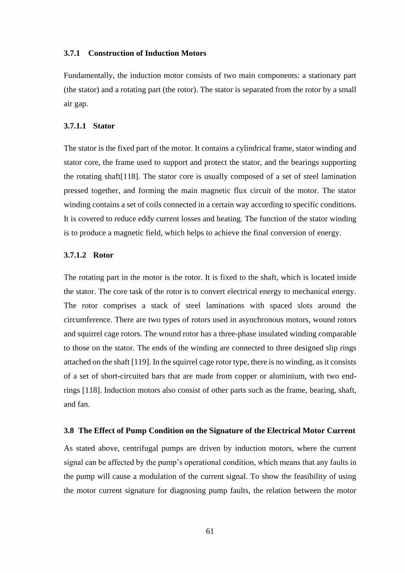
61

3.7.1 Construction of Induction Motors

Fundamentally, the induction motor consists of two main components: a stationary part

(the stator) and a rotating part (the rotor). The stator is separated from the rotor by a small

air gap.

3.7.1.1 Stator

The stator is the fixed part of the motor. It contains a cylindrical frame, stator winding and

stator core, the frame used to support and protect the stator, and the bearings supporting

the rotating shaft[118]. The stator core is usually composed of a set of steel lamination

pressed together, and forming the main magnetic flux circuit of the motor. The stator

winding contains a set of coils connected in a certain way according to specific conditions.

It is covered to reduce eddy current losses and heating. The function of the stator winding

is to produce a magnetic field, which helps to achieve the final conversion of energy.

3.7.1.2 Rotor

The rotating part in the motor is the rotor. It is fixed to the shaft, which is located inside

the stator. The core task of the rotor is to convert electrical energy to mechanical energy.

The rotor comprises a stack of steel laminations with spaced slots around the

circumference. There are two types of rotors used in asynchronous motors, wound rotors

and squirrel cage rotors. The wound rotor has a three-phase insulated winding comparable

to those on the stator. The ends of the winding are connected to three designed slip rings

attached on the shaft [119]. In the squirrel cage rotor type, there is no winding, as it consists

of a set of short-circuited bars that are made from copper or aluminium, with two end-

rings [118]. Induction motors also consist of other parts such as the frame, bearing, shaft,

and fan.

3.8 The Effect of Pump Condition on the Signature of the Electrical Motor Current

As stated above, centrifugal pumps are driven by induction motors, where the current

signal can be affected by the pump’s operational condition, which means that any faults in

the pump will cause a modulation of the current signal. To show the feasibility of using

the motor current signature for diagnosing pump faults, the relation between the motor

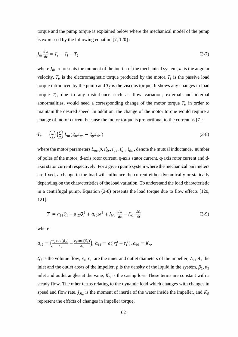
62

torque and the pump torque is explained below where the mechanical model of the pump

is expressed by the following equation [7, 120] :

𝐽𝑚𝑑𝜔

𝑑𝑡= 𝑇𝑒 − 𝑇𝑙 − 𝑇𝜉 (3-7)

where 𝐽𝑚 represents the moment of the inertia of the mechanical system, 𝜔 is the angular

velocity, 𝑇𝑒 is the electromagnetic torque produced by the motor, 𝑇𝑙 is the passive load

torque introduced by the pump and 𝑇𝜉 is the viscous torque. It shows any changes in load

torque 𝑇𝑙, due to any disturbance such as flow variation, external and internal

abnormalities, would need a corresponding change of the motor torque 𝑇𝑒 in order to

maintain the desired speed. In addition, the change of the motor torque would require a

change of motor current because the motor torque is proportional to the current as [7]:

𝑇𝑒 = (3

2) (

𝑃

2) 𝐿𝑚(𝑖𝑑𝑟

′ 𝑖𝑞𝑠 − 𝑖𝑞𝑟′ 𝑖𝑑𝑠 ) (3-8)

where the motor parameters 𝐿𝑚, p, 𝑖𝑑𝑟′ , 𝑖𝑞𝑠, 𝑖𝑞𝑟

′ , 𝑖𝑑𝑠 , denote the mutual inductance, number

of poles of the motor, d-axis rotor current, q-axis stator current, q-axis rotor current and d-

axis stator current respectively. For a given pump system where the mechanical parameters

are fixed, a change in the load will influence the current either dynamically or statically

depending on the characteristics of the load variation. To understand the load characteristic

in a centrifugal pump, Equation (3-8) presents the load torque due to flow effects [120,

121]:

𝑇𝑙 = 𝑎𝑡1𝑄𝑖 − 𝑎𝑡2𝑄𝑖2 + 𝑎𝑡0𝜔2 + 𝐽𝑀𝑣

𝑑𝜔

𝑑𝑡− 𝐾𝑄

𝑑𝑄𝑖

𝑑𝑡 (3-9)

where

𝑎𝑡2 = (𝑟2cot (𝛽2)

𝐴2−

𝑟2cot (𝛽1)

𝐴1), 𝑎𝑡1 = 𝜌( 𝑟2

2 − 𝑟12), 𝑎𝑡0 = 𝐾𝑛.

𝑄𝑖 is the volume flow, 𝑟1, 𝑟2 are the inner and outlet diameters of the impeller, 𝐴1, 𝐴2 the

inlet and the outlet areas of the impeller, ρ is the density of the liquid in the system, 𝛽1, 𝛽2

inlet and outlet angles at the vane, 𝐾𝑛 is the casing loss. These terms are constant with a

steady flow. The other terms relating to the dynamic load which changes with changes in

speed and flow rate. 𝐽𝑀𝑣 is the moment of inertia of the water inside the impeller, and 𝐾𝑄

represent the effects of changes in impeller torque.

63

The equation above shows that abnormalities or defects on the impeller due to cavitation,

erosion or blockage will cause changes in pressure, flow rates and corresponding

oscillations, which in turn lead to changes in both static motor torque and dynamic motor

torque. These will affect both the static and dynamic elements of the motor current data.

This implies that both static and the dynamic current components could be valuable for

fault detection and diagnosis of these faults.

Thus the motor current signature could be valuable for detection and diagnosis of pump

faults. In addition, the flow rate will be adjusted by vanes inside each vane exhibits

impulsive behaviour, and these will be reflected into the current signature through the load

torque. Therefore, investigating these changes in the motor current signals will allow the

monitoring of the pump condition.

3.8.1 Current Responses for Normal operating of the pump

For simplicity and a better understanding, the electromagnetic operation of the electrical

motor (healthy condition) one phase of the three phases of a power supply system is

considered. The current signal in this phase, phase A, for the healthy motor can be

represented as [122, 123].

2 cos(2 )A s Ii I f t = − (3-10)

The magnetic flux in the motor stator is

2 cos(2 )A sf t = − 3-11)

The electrical, magnetic torque produced by the interaction between the current and the

flux, it can be presented as:

3 sin( )IT P I = − (3-12)

where P is the number of pole pairs of the phase, and I is the RMS amplitude of the stator

fundamental current and φ is RMS of the linkage flux, while I is the phase of the current

and is the flux phase, and sf is the fundamental frequency of the motor.

64

3.8.2 Current Responses for Abnormal operating of the pump

As explained above the occurrence of any defects in the rotational components, such as

the impeller and bearings will lead to extra torque component oscillations around the

torque of the motor. Given the additional torque is of amplitude ΔT, and is sinusoidal with

a frequency, kf , it follows that the current amplitude kI and phase k , resulting from the

oscillatory torque can be obtained from Equation (3-13) [124, 125]:

3 sin[2 ( ) ]k k I kT P I f t = − − − (3-13)

The change of the torque will cause a fluctuation in the angular speed given by;

23cos[2 ( ) ]

2

k

k I k

k

P IPTdt f t

J f J

= = − − − −

(3-14)

where J is the inertia of the system.

This change in angular speed results in phase modulation of the linkage flux and Equation

(3-11) becomes;

(3-15)

where 2

2 2

3

4

k

k

P I

f J

= .

This demonstrates that the flux has a nonlinear effect due to the defect in the rotor system.

An electromagnetic force (EMF) will be generated by the nonlinear interaction of flux,

and therefore, a nonlinear current signal will be induced in the stator.

For a very small Δαk we have cos (Δαk) ≈ 1 and sin (Δαk) ≈ Δαk, and the linkage flux can

be expressed as:

65

(3-16)

From equation (3-16), the flux comprises both the fundamental and sidebands aroundsf .

The current can be then be derived from the motor equivalent circuit:

(3-17)

where φ is the angular displacement at supply frequency, Il and Iu are the RMS amplitudes

of the resulting sidebands (lower and upper) around the current produced by the healthy

motor, which are induced by the back-EMF voltages produced by the flux variations at

frequencies of 𝑓𝑠 − 𝑓𝑘 and 𝑓𝑠 + 𝑓𝑘.

This basic expression shows that, in principle, the current signal in the driving motor can

be used to detect the presence of a downstream mechanical fault, and has been widely used

for CM. However, the equations are based on an idealised motor, and certain simplifying

assumptions, and serve as a guide. Equations are an approximation of the real situation

when actual faults are present. The equations show that changes are to be expected, and

the faults can be detected. This can be based on tracking the characteristic fault frequency

or calculating the variation content in the current energy in particular frequency ranges to

determine the presence of mechanical defects.[126]. However, other characteristic features

may also be present in the signal.

Thus, an advanced signal processing technique is required to analyse and demodulate the

motor current signal for detection of mechanical defects. It is hypothesised that data-driven

techniques could form a more robust tool to link fault and signal, to increase the

effectiveness of MCSA for extracting the weak current signatures generated by faults from

the motor current signals in order to yield superior detection and diagnosis of faults. Such

66

an approach could provide the benefit of enabling us to identify links which do not

necessarily correspond to the above analysis, e.g., structural changes in one component

could be related to functional changes in another.

3.9 Key Findings

Due to their simplicity of structure and use, and capability of operating at high speed with

a steady output flow for long periods, centrifugal pumps are widely used in numerous

process industries such as petrochemical, agriculture, and chemical, as well as in water

purification plants, Such pumps are often deployed in critical areas, where any defects that

occur will not only reduce plant efficiency but could lead to a production breakdown. To

preserve pump efficiency and reliability, and to ensure optimum operating conditions, it is

crucial to monitor the pump’s condition and detect faults at the earliest, so that appropriate

actions can be taken in good time to facilitate pump maintenance.

During pump operation, the interaction between the flow and torsional and rotational

oscillations of the drive shaft will generate changes in the air-gap’s magnetic field. This

means that the motor current responds to any mechanical defects during the pump

operation. Thus, the MCSA provides a reasonable and attractive technique for monitoring

the condition of the pump. The literature review revealed that the most common defects in

centrifugal pumps are bearing faults and impeller blockage [100, 102]. Thus these were

the faults chosen for investigation in this study. The next chapter explains the data analysis

methods in more details.

67

Techniques for Extracting Condition

Monitoring Information

This chapter provides a review of the literature on methods used for extracting and

analysing diagnostic information for machine CM. It presents the data analytic methods

that are widely used for detecting faults in machines; it discusses their algorithms,

strengths and limitations. The chapter focuses mainly on relevant MCSA methods in order

to obtain effective features to detect and diagnose different centrifugal pump faults. These

explanations are introduced to help understand the techniques that will be used in the

succeeding chapters of this thesis.

68

4.1 Introduction

To achieve reliable condition monitoring and fault diagnosis results, appropriate methods

for analysing and assessing the abnormal condition of the rotating machine are required.

Several signal processing techniques have been used to analyse and interpret waveform

data to extract useful information for a further diagnostic purpose[127].

The current signal acquired from the machine is often contaminated by noise and affected

by machine operating condition. Thus, they require suitable and more reliable techniques

for extracting features related to the machine condition. Typically, there are three different

ways to look into the signal: time domain analysis, frequency domain and time-frequency

domain. In this research, advanced data analysis techniques have been used to improve

the diagnostic method for various centrifugal pump defects based on the motor current

signature analysis.

4.2 Time Domain Analysis

The most basic analysis of a signal is based on its time domain waveform. It is a series of

discrete values sampled over a period of time, invariably at regular intervals which are at

a frequency at least twice as fast as the highest frequency of interest. In this technique,

characteristic features can be extracted based on the amplitude of the signals; these features

include root mean square, mean, peak values, standard deviation, and so on. These features

provide a means of evaluating a machine’s condition [10].

Figure 4-1 shows the time domain waveform of the current of a motor driving a centrifugal

pump for different pump conditions with a fixed flow rate. The two signals are for the

baseline (healthy) pump condition and the pump with a seeded fault introduced into the

inner ball race of the pump bearing. It is clear that the waveforms show changes in the

peak amplitudes according to the different pump conditions. It can be seen from the figure

that the signals exhibit amplitude modulation.

69

Figure 4-1 Time domain current signal for flow rate 350 l/min

However, it is hard to assess the condition of the centrifugal pump from the signal

waveform alone, especially when the pump works under abnormal operation. Thus, there

is a need for calculating some of statistical parameters based on the time domain

information for assessing the real condition and behaviour of the pump. Statistical

parameters such as root mean square, crest vector, and kurtosis [128] are used for

diagnosing pump faults. It has been shown that there exists a correlation between the

amplitude of these statistical parameters, and the damage occurred in particular

components of the machine [129]. Some common statistical features are described in the

next sub-section:

4.2.1 Root Mean Square

Root mean square (RMS) represents the overall energy content of the signal. RMS is the

most common feature in the time domain of the signal and is also an effective parameter

for detecting faults in machines [130]. It can be calculated by the formula [131]:

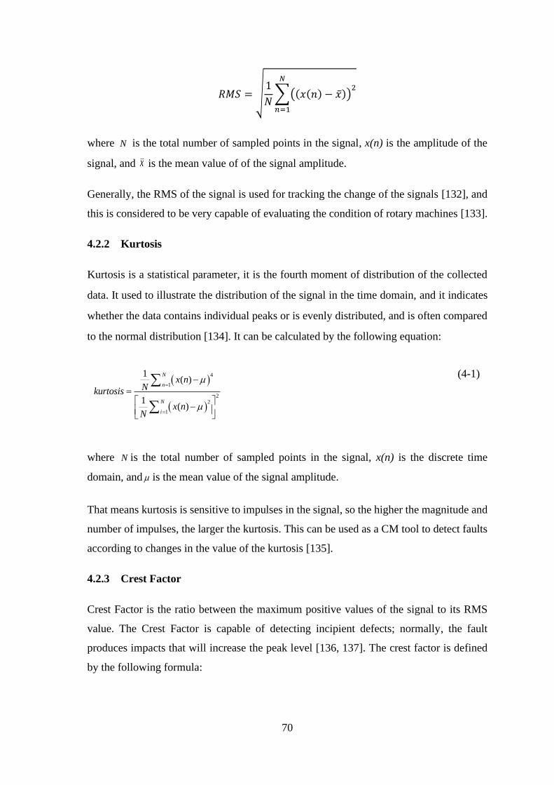
70

𝑅𝑀𝑆 = √1

𝑁∑((𝑥(𝑛) − �̅�))

2𝑁

𝑛=1

where N is the total number of sampled points in the signal, x(n) is the amplitude of the

signal, and x is the mean value of of the signal amplitude.

Generally, the RMS of the signal is used for tracking the change of the signals [132], and

this is considered to be very capable of evaluating the condition of rotary machines [133].

4.2.2 Kurtosis

Kurtosis is a statistical parameter, it is the fourth moment of distribution of the collected

data. It used to illustrate the distribution of the signal in the time domain, and it indicates

whether the data contains individual peaks or is evenly distributed, and is often compared

to the normal distribution [134]. It can be calculated by the following equation:

(4-1)

where N is the total number of sampled points in the signal, x(n) is the discrete time

domain, and is the mean value of the signal amplitude.

That means kurtosis is sensitive to impulses in the signal, so the higher the magnitude and

number of impulses, the larger the kurtosis. This can be used as a CM tool to detect faults

according to changes in the value of the kurtosis [135].

4.2.3 Crest Factor

Crest Factor is the ratio between the maximum positive values of the signal to its RMS

value. The Crest Factor is capable of detecting incipient defects; normally, the fault

produces impacts that will increase the peak level [136, 137]. The crest factor is defined

by the following formula:

( )

( )

4

1

22

1

1( )

1( )

N

n

N

i

x nNkurtosis

x nN

=

=

−

=

−

71

max rms

xCrest factor

x= (4-2)

where maxx the absolute maximum value of the acquired signal, rmsx is the RMS value.

From the above equation, the crest factor has a direct relationship with peak value and an

inverse relationship with the RMS value. When peak value increases the value of the crest

factor also increases. Therefore, the crest factor is an effective indicator primarily when

the signal is “impulsive” [137].

4.3 Frequency Domain Analysis

In this analysis, the time domain signal is transformed to the frequency domain. The

frequency content of the signal (spectrum analysis) is very important for analysing and

assessing the acquired signals. Frequency domain analysis identifies precise frequency

components in the frequency spectrum or in a specific frequency range. The most

commonly used method for transforming time domain samples to the frequency domain is

the Discrete Fast Fourier Transform (DFFT) [10, 138].

Let x(t) be the continuous signal for N samples: x(0), x(1) ..... x(N-1)

The DFFT = ∑ 𝑥(𝑛) 𝑒−2𝑗𝜋𝑓𝑡𝑥=𝑁−1𝑥=0

According to the Nyquist theorem, the sampling frequency must be at least twice the

highest frequency of interest [139].

All components related to the machine’s operation can be seen in the frequency domain.

The characteristic features or patterns present in the frequency domain are very useful for

identifying the characteristics and behaviour of the system [140]. It has been found that

the most defects generate modulation sidebands around the fundamental frequency of a

rotating machine. Also, some faults are associated with particular defect frequencies (and

their harmonics), the magnitude of these specific frequencies and sidebands will often

afford meaningful information on the condition of the machine [122, 141].

However, FFT has limitations as it suffers from frequency leakage, which makes it difficult

to distinguish the signal of a healthy condition from a faulty one. The DFFT is based on

samples of short duration, whereas the original signal is likely to have extended over a

72

considerably longer time. So, for the DFFT to produce representative results, it is assumed

the original signal is stationary. The inevitable consequence is that information is lost when

transforming a time domain signal into a frequency-domain signal. To minimise, but not

eliminate, the error, a windowing function is used which can itself introduce further error.

Nevertheless, the DFFT has proved to be an immensely successful and useful tool in the CM

of rotating machinery.

Another limitation of this method is its frequency resolution, the total time of signal

acquisition has a major effect on the resolution. To overcome this particular limitation,

data of sufficient length should be captured [142]. Thus, it is preferable to utilize advanced

signal processing techniques such as wavelets and other adaptive methods for more in-

depth analysis of the signal [143].

4.4 Time-Frequency Domain

Both time domain and frequency domain analysis are useful for analysing and extracting

meaningful information to evaluate the condition of some rotating machines that generate

stationary signals. However, they are limited when analysing non-stationary signals and

cannot explain the change of the signal over time, particularly when the signal is subject

to frequency modulation [144].

In order to overcome these drawbacks, methods have been developed based on joint time-

frequency analysis whereby nonstationary and non-linear signals can be analysed.

As the current signal from the centrifugal pump with a seeded fault will be nonstationary

in behaviour, it is worth examining this signal using time-frequency analysis. There are

many techniques based on the time-frequency domain, such as:

4.4.1 Short Time Fourier Transform

Short Time Fourier Transform (STFT) is based on the idea of using a moving window

over the time domain data to get the stationary component from the nonstationary signal.

The process involves dividing the entire time domain data into a set of segments, then

applying the Fourier Transform to each short signal segment one by one [145]. The process

of the STFT can be defined by a localised function:

73

𝑆𝑇𝐹𝑇(𝑡, 𝑓) = ∫ 𝑥(𝑡)𝑤(𝑡 − 𝜏)𝑒−𝑗2𝜋𝑓𝑡 𝑑𝑡∞

−∞ (4-3)

where x(t) is the original signal, w(t) is the window function and 𝜏 is the time-shift

parameter.

The main drawback of this transform method is the limit imposed by high redundancy.

Another limitation is that the time-frequency resolution is seriously affected by the size of

the window. In the STFT method, even though the method can analyse nonstationary

signal more effectively than the traditional FFT technique, it still suffers from frequency

resolution issues. Analysing the signal by STFT is limited by the constraint of having to

use a window of fixed duration. The difficulty is to choose the best window length for a

signal that contains both low and high frequencies at the same time since, if a long window

is used, there will be better frequency resolution, but poorer time resolution and vice versa

[146]. For that reason, STFT is more appropriate for analysing quasi-stationary signals

rather than real-life non-stationary signals

4.4.2 Wavelet Transform

The wavelet transform (WT) decomposes the signal utilising a variable length window.

The WT uses a mathematical function, called a wavelet function to replicate the signal

[147]. Unlike the STFT, it is a robust localisation method as it provides a multi-resolution

window that depends mainly on the frequency components of the signal [146].

Mathematically, it can be defined as follows [148]:

*

,

1( , ) ( )s

ta f t dt

aa

−

− =

(4-4)

where a is the scale parameter, φ the shift parameter, and ‘*’ represents the complex

conjugation operation, and ψ(t) is the wavelet function.

Formula (4-4) is also called the continuous WT, as it employs a continuous range for both

parameters of scale and shift. Moreover, it has the ability to analyse nonstationary signals,

whereas the Fourier transform is unable to do so. Unlike Fourier analysis where the

window is of constant length, in the WT, the size of the window depends on the scale and

the shift parameter [149].

74

4.5 Envelope Analysis

Envelope analysis or the method of demodulation is based on the extraction of low-

frequency components from the signal, which is modulated by a high carrier signal. This

method has been employed for detecting faults such as bearing defects and cavitation in

pumps [150]. It is used for demodulating the signals following the process explained in

Figure 4-2. The envelope of an analytic signal is determined by the equation [151]:

2 2 e(t)= ( ) [ ( )]x t H x t+ (4-5)

where 𝐻[𝑥(𝑡)] it is the Hilbert transformation of the given signal 𝑥(𝑡).

Figure 4-2 Envelope Analysis Method [150].

The process starts with filtering the raw data of the current signal by means of a bandpass

filter to specify the frequency range of interest. The next step uses the Hilbert Transform

to rectify the signal. Then the FFT is applied to obtain the envelope spectrum [150]. The

envelope contributes significantly to reduce the noise and helps to maximise the signal to

noise ratio. Also, the amplitude values of the signal become more apparent in the envelope

spectrum, which is not evident in the results for the FFT [152].

4.6 Empirical Mode Decomposition

Empirical Mode Decomposition (EMD) is an adaptive approach used to analyse the signals

based on their local characteristics. EMD is a data-driven and robust decomposition

method for analysing nonstationary and non-linear signals. Huang, et al., introduced it in

1998[153]. The fundamental concept of the EMD is decomposing complicated signal

iteratively into a number of narrowband components of intrinsic mode functions (IMFs)

which remain in the time domain, and are of the same duration as the original signal, which

means information related to the frequency content of the signal is retained [74].

Unlike STFT and WT, data-driven EMD is a robust technique. Compared with the STFT,

the WT is more appropriate for analysing non-stationary signals, by means of dilation and

translation, it utilizes a variable length window that depends on both the scale and the

75

shifting processes. The wavelet has the major disadvantage that the analysis results depend

on the a priori choice of an appropriate wavelet function, known as the ‘mother wavelet’.

The challenge here lies in choosing a suitable function to capture the required

characteristics of the data [154].

The limitations mentioned above regarding analysis of non-stationary signals using a

STFT can be overcome by using EMD, as it is a data-driven technique. EMD is an

appropriate tool for analysing non-linear and non-stationary signals because the foundation

functions are determined from the data itself [74, 155]. In EMD, because there is no need

to select a basis function for the decomposition procedure. This method can obtain the

characteristics of the signals more precisely than the traditional FFT and WT methods.

4.6.1 Empirical Mode Decomposition Algorithm

The main function of the EMD decomposes the given signal x(t) into several modes of

oscillation. There are two essential conditions to be satisfied by an intrinsic mode function

(IMF):

(i) In the complete data series, the total number of extrema points and the zero

crossings must be equal, or at most differ by 1.

(ii) The mean constructed from the envelopes must be symmetric in nature [153].

76

Figure 4-3 Flowchart of the EMD algorithm [156].

Figure 4-3 presents the algorithm of the EMD, which can be explained as follows [155]:

1. Identify both the local extrema (maxima and minima) of the original signal 𝑥(𝑡).

2. Determine the upper 𝑒𝑢𝑝(𝑡) and lower 𝑒𝑙𝑜𝑤(𝑡) envelopes using a cubic spline

interpolation by connecting all recognized maxima and minima points.

3. Calculate the mean, ( )im t of the envelopes.

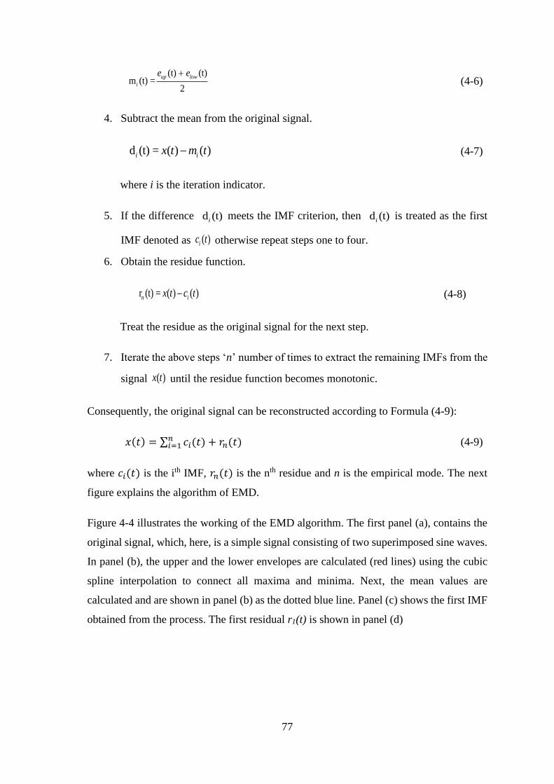
77

(t) (t) m (t) =

2

up low

i

e e+ (4-6)

4. Subtract the mean from the original signal.

d (t) = ( ) ( )i ix t m t− (4-7)

where i is the iteration indicator.

5. If the difference d (t)i meets the IMF criterion, then d (t)i

is treated as the first

IMF denoted as ( )ic t otherwise repeat steps one to four.

6. Obtain the residue function.

r (t) = ( ) ( )n ix t c t− (4-8)

Treat the residue as the original signal for the next step.

7. Iterate the above steps ‘n’ number of times to extract the remaining IMFs from the

signal ( )x t until the residue function becomes monotonic.

Consequently, the original signal can be reconstructed according to Formula (4-9):

𝑥(𝑡) = ∑ 𝑐𝑖(𝑡) + 𝑟𝑛(𝑡)𝑛𝑖=1 (4-9)

where 𝑐𝑖(𝑡) is the ith IMF, 𝑟𝑛(𝑡) is the nth residue and n is the empirical mode. The next

figure explains the algorithm of EMD.

Figure 4-4 illustrates the working of the EMD algorithm. The first panel (a), contains the

original signal, which, here, is a simple signal consisting of two superimposed sine waves.

In panel (b), the upper and the lower envelopes are calculated (red lines) using the cubic

spline interpolation to connect all maxima and minima. Next, the mean values are

calculated and are shown in panel (b) as the dotted blue line. Panel (c) shows the first IMF

obtained from the process. The first residual r1(t) is shown in panel (d)

78

Figure 4-4 Illustration of the EMD method [157].

EMD has been employed to examine the signal behaviour for identifying the defects in

rotating machine parts such as rolling bearings, gears, stators and rotors. Lin, et al., [158]

extracted IMFs from the vibration signal in order to diagnose the condition of a driving

shaft. Miao, et al., [159] utilized independent component analysis combined with EMD to

diagnose bearing defects from acquired vibration data. The set of IMFs was chosen

depending on the energy content of the frequency spectrum, followed by independent

component analysis whereby the fault signatures of both inner and outer races were

identified. Georgoulas, et al., [160] introduced a diagnostic approach by combining EMD

and pattern recognition methods for the detection of broken-bar faults in an electric motor,

where the complex IMF was converted into a discrete time series, then classification was

achieved using hidden Markov models.

Sun et al. [59] investigated pump cavitation using the EMD-based Hilbert-Huang

transform for analysing vibration and current data. The analysis showed that the unsteady

flow responsible for the torque oscillations due to the cavitation process can contribute to

variations in the energy of the vibration and current signals, and the RMS of the IMF was

79

capable of detecting and diagnosing the presence of the pump cavitation. Yunlong and

Peng [161] utilised EMD for decomposing the vibration signals of a centrifugal pump in

different states of health, and later a support vector machine (SVM) was employed to

distinguish the different cases and diagnose the faults.

Ali et al. [162] have applied an automated fault diagnosis technique for bearings based on

an artificial neural network (ANN) and EMD, where statistical parameters from the time

domain were evaluated and successfully employed to train the ANN technique to classify

bearing faults. The analysis results proved its reliability and effectiveness in categorising

the bearing defects. Bin, at el., [163] proposed wavelet packet decomposition using EMD

combined with an ANN; a set of feature frequencies were extracted from the vibration

signal for detection of a crack in rotating machinery. The results show that the proposed

method can effectively extract features for diagnosing the early fault of rotating

machinery. Liu, et al., [164] applied EMD and Hilbert spectrum to analyse the vibration

data for localised gearbox fault diagnosis and found that EMD algorithms have superior

performance compared to the continuous WT for enhancing the transients induced by a

gear tooth crack.

The EMD method is appropriate for diagnosing the condition of a machine where the faults

impose amplitude modulation on the frequency signal from the rotating machine

components[165].

With centrifugal pump operation, the modulation of the current signal becomes more

noticeable as the flow rate increases. Also, the current signal is invariably contaminated

by a variety of noise, and most of which will be generated by non-linear processes. As

EMD has the advantage of being able to handle nonlinear and nonstationary signals, it

allows the modulated signals to be decomposed into different simple intrinsic modes of

oscillation, so that the characteristics of the signal could be revealed clearly and noise

components are filtered. Thus, the EMD method is deemed suitable to be used in this

research for decomposing the modulated current signals into mono-components that

highlight the periodic components of interest-specific frequencies, and extract useful

features for more accurate fault detection.

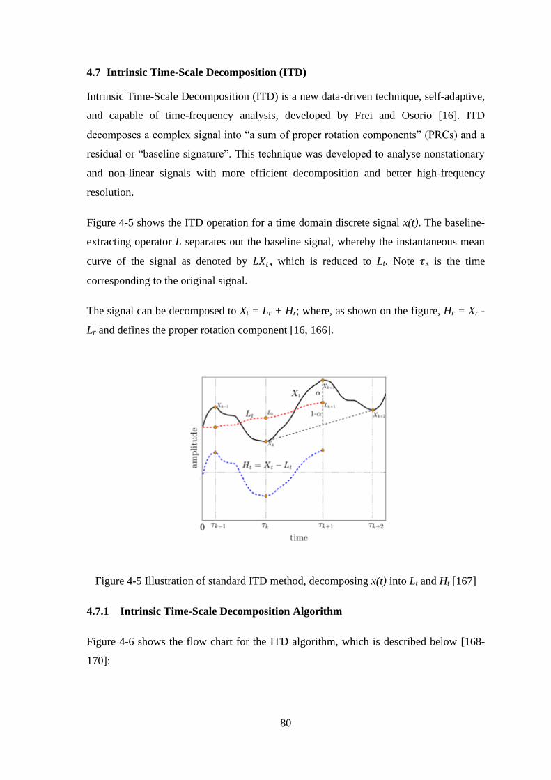
80

4.7 Intrinsic Time-Scale Decomposition (ITD)

Intrinsic Time-Scale Decomposition (ITD) is a new data-driven technique, self-adaptive,

and capable of time-frequency analysis, developed by Frei and Osorio [16]. ITD

decomposes a complex signal into “a sum of proper rotation components” (PRCs) and a

residual or “baseline signature”. This technique was developed to analyse nonstationary

and non-linear signals with more efficient decomposition and better high-frequency

resolution.

Figure 4-5 shows the ITD operation for a time domain discrete signal x(t). The baseline-

extracting operator L separates out the baseline signal, whereby the instantaneous mean

curve of the signal as denoted by 𝐿𝑋𝑡, which is reduced to Lt. Note 𝜏k is the time

corresponding to the original signal.

The signal can be decomposed to Xt = Lr + Hr; where, as shown on the figure, Hr = Xr -

Lr and defines the proper rotation component [16, 166].

Figure 4-5 Illustration of standard ITD method, decomposing x(t) into Lt and Ht [167]

4.7.1 Intrinsic Time-Scale Decomposition Algorithm

Figure 4-6 shows the flow chart for the ITD algorithm, which is described below [168-

170]:

81

Figure 4-6 Flow chart of ITD algorithm

1. The process starts with calculating the extreme points (𝜏k, Xk) for the given signal X(t)

that needs to be decomposed. Xt is the amplitude value of the untreated points, and k =

0, 1, 2….

2. The baseline signal is then obtained based on the extreme points, and the baseline

signal is separated from the original signal with the help of baseline-extracting

operators Lt and Ht determined over the time interval [0, 𝜏k], where the signal Xt exists

82

in the interval [0, 𝜏k+2]. Then for the range of (𝜏k, 𝜏k+1], define the baseline-extracting

operator 𝐿t which is a piecewise linear function, realized from Equation (4-10):

1

1

1

( ), ( , ]k k

t t k t k k k

k k

L LLX L L X X t

X X +

+

+

−= = + −

− (4-10)

where

1

1 2 1

2

( ) (1 )k k

k k k k k

k k

L X X X X

+

+ + +

+

−= + − + −

− (4-11)

and 0 < α < 1. Usually α is around 0.5.

3. Obtain the baseline signal 𝐿𝑡 in order to maintain the monotonicity of 𝑋𝑡 between the

extrema points.

4. For extracting the PRC of the signal, the operator 𝐻𝑡 determined as:

𝐻𝑡 = 𝑋𝑡 − 𝐿𝑡 (4-12)

5. Then repeat the previous steps by adopting 𝐻𝑡 as 𝑋𝑡 until 𝐻𝑡 is accepted as 𝑃𝑅𝐶1 (𝑡).

6. Compute the residual signal, 𝑟(𝑡), by subtracting 𝑃𝑅𝐶1 (𝑡) from 𝑋(𝑡).

𝑟(𝑡) = 𝑋(𝑡) − 𝑃𝑅𝐶1(𝑡) (4-13)

Now treat the residual as the given signal.

7. Considering r(t) as X(t) the previous steps are repeated until the base signal becomes a

monotonic function, or when the signal contains less than three extrema points, the

decomposition end, and the set of PRCs with a residual will enable the original signal

to be reconstructed as:

𝑋𝑡 = ∑ 𝑃𝑅𝐶𝑖𝑝𝑖=1 (𝑡) + 𝑟𝑝 (4-14)

where the p is the number of the obtained PRCs.

83

ITD has the ability to overcome some of the limitations of wavelet transformations, where

aspects of the signal characteristics may be lost. With WTs, it is hard to obtain a detailed

description of the signal because WTs are based on the use of a predefined mother wavelet

which is not self-adapting [171].

The ITD method can utilize more local characteristic information of the signal as the

process of construct the baseline signal depends on the linear interpolation rather than

cubic spline interpolation that used in EMD. Therefore, ITD has evident advantages in the

end effects and envelope, thus, the PRC retain almost all extrema information of the

original signal [172].

ITD has been used for processing non-linear signals for CM. Feng, et al., [168] have used

ITD to decompose the vibration signals from a planetary gearbox into a set of mono-

components for demodulation and further analysis. An, et al.,[173] applied ITD for fault

diagnosis of wind turbine bearings using measured vibration signals. These researchers

applied the ITD to extract the frequency centres of the first PRC as a fault features vector

and applied the nearest neighbour algorithm to classify the operational condition of these

bearings.

Aijun et al. [174] have diagnosed wind turbine gearbox faults by combining ensemble

ITD, with WT to analyse vibration signals, and then adopting correlation to identify the

working conditions and fault types. The vibration data were acquired from accelerometers

placed on the drive shaft of the gear. Liu, et al., [175] applied ITD to analyse the vibration

data from a diesel engine for fault diagnosis. A set of features was extracted from the time

and frequency domains for the first several PRCs, and then a multistage relevant vector

machine (RVM) model was constructed and employed to diagnose diesel engine faults.

Jianbo and Haiqiang [172] applied a combined method based on the ITD and sparse coding

shrinkage to extract a weak fault feature contaminated by background noise from bearing

vibration signals.

Lin, et al., [176] introduced an approach for detecting rolling element bearing faults based

on the ITD method. First, the spectral kurtosis was used to investigate the vibration data.

Then ITD was used to decompose the filtered signal by kurtogram, and then envelope

analysis was carried out to demodulate the decomposed signals and extract the

characteristics of the fault.

84

Although ITD has been shown to be an effective way of processing vibration signals for

machine fault detection and diagnosis, it is noted that very few studies have been carried

out using ITD for monitoring pump condition.

There is no significant evidence has been found in the literature of the use of ITD for

MCSA for such applications. This research will focus on detecting and diagnosing

common centrifugal pump faults using ITD.

4.8 Key Findings

For assessing the machine condition different detection and diagnosis techniques can be

applied to extract useful information, the simplest way from signal processing is time-

domain analysis, that present the raw data as a function of time, also spectrum analysis is

most widely used for analysing and assessing the acquired signals, it is limited when

analysing the non-stationary and non-linear signals for fault diagnosis. As most of the

machine faults typically generate non-stationary components in the signals, which contain

critical information about machinery condition. Data-driven techniques such as EMD and

ITD allow multiple-components of signal to be decomposed into different simple intrinsic

components where the effective features can be extracted and used for detecting and

diagnosing the faults.

85

Machine Learning for Fault Detection and

Diagnosis

This chapter presents a review of Machine Learning in the context of this research. It starts

with an introduction to key machine learning algorithms and provides a comprehensive

approach on how a supervised classification method can be constructed. The SVM

algorithm is examined in more detail as it will be used as a tool in this study for

classification and to differentiate different types of centrifugal pump faults. Finally, the

chapter describes multi-class support vector machines.

86

5.1 Introduction

Machine Learning (ML) can be defined as a group of computational techniques that focus

on learning from past experiences to make a prediction for the future. The main goals of

ML are (i) to construct an accurate model that can be used to make predictions for new

data [177], and (ii) to design robust algorithms to achieve this prediction when dealing

with large data set [178].

Various ML have methods emerged from the efforts of psychologists developing theories

and models for animal and human learning. ML is capable of learning from experience,

and analysis of acquired data, which gives it the ability to improve itself. Therefore, by

using ML, the efficiency and effectiveness of systems can be improved [3]. ML has been

utilized in numerous tasks including, for instance, regression, clustering and classification.

Classification is one of the best-known implementations of ML. It is a method for

determining a class label for new input data, where the class label is designated as one of

a known set of classes using a model based on ML algorithms [179]. In this study, the

classification task is used to distinguish faults based on SVM algorithm.

5.2 Types of Machine Learning

In general, ML can be classified into three types: supervised learning, unsupervised

learning, and semi-supervised learning [180]. A brief description of these types is provided

below:

Supervised learning: The primary goal of supervised machine learning is constructing

and training the model based on a labelled dataset. The labelled dataset comprises of input

and output parameters. The model is used to predict or assign class labels to new data for

which the class label is unknown [181]. The broad purpose of supervised learning is as a

classification task, where acquired data will be classified in accordance with the training

model, as shown in Figure 5-1.

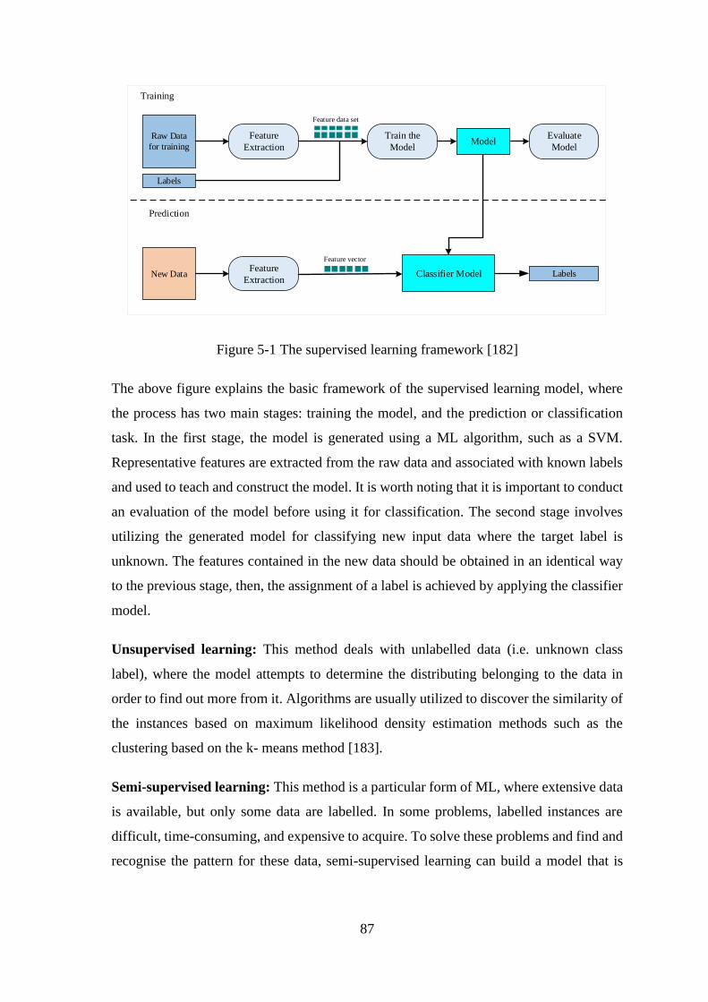
87

Figure 5-1 The supervised learning framework [182]

The above figure explains the basic framework of the supervised learning model, where

the process has two main stages: training the model, and the prediction or classification

task. In the first stage, the model is generated using a ML algorithm, such as a SVM.

Representative features are extracted from the raw data and associated with known labels

and used to teach and construct the model. It is worth noting that it is important to conduct

an evaluation of the model before using it for classification. The second stage involves

utilizing the generated model for classifying new input data where the target label is

unknown. The features contained in the new data should be obtained in an identical way

to the previous stage, then, the assignment of a label is achieved by applying the classifier

model.

Unsupervised learning: This method deals with unlabelled data (i.e. unknown class

label), where the model attempts to determine the distributing belonging to the data in

order to find out more from it. Algorithms are usually utilized to discover the similarity of

the instances based on maximum likelihood density estimation methods such as the

clustering based on the k- means method [183].

Semi-supervised learning: This method is a particular form of ML, where extensive data

is available, but only some data are labelled. In some problems, labelled instances are

difficult, time-consuming, and expensive to acquire. To solve these problems and find and

recognise the pattern for these data, semi-supervised learning can build a model that is

Training

Raw Data

for training

Feature

Extraction

Labels

ModelTrain the

Model

Classifier Model LabelsFeature

ExtractionNew Data

Feature data set

Feature vector

Evaluate

Model

Prediction

88

useful for large sets of combined unlabelled and labelled data. This method sits between

supervised and unsupervised learning in terms of applicability [184].

Recently, several machine-learning algorithms have been utilized in the field of CM, such

as decision trees, neural networks, naive Bayes, and so on. The main goal of intelligent

diagnostic methods is to analyse the gathered data and automatically provide an accurate

diagnosis. Such a process has become a new trend in the field of CM [185]. It used to help

diagnose the condition of rotating machines, providing a more automatic and intelligent

method in which the accuracy of the CM procedure will increase. In this context, many

algorithms have been shown to yield effective results for fault detection and diagnosis.

The utilisation of ML for detecting and diagnosing the defects of pumps has become a

more popular technique in comparison to conventional methods for signal processing, and

a more attractive area for researchers, in particular where it can be merged with advanced

data analysis techniques for enhancing the CM of rotating machines [3, 186].

However, the successful employment of ML methods for detecting and diagnostic machine

faults depend on such factors as the characteristics of the acquired raw data, the quality of

processed datasets, and the extraction of suitable diagnostic features. Specifically, it is

critical to extract and select reliable and appropriate features to be used for training the

classification model, features which can accurately describe the pattern of the current

signal so that the output of the learning model will enhance the overall CM process.

5.3 Support Vector Machine

The Support Vector Machine (SVM) is a machine-learning algorithm used for both

classification and regression tasks. This method is founded on the theory of statistical

learning and was introduced in 1995 by Cortes and Vapnik [187]. SVM defines an optimal

separating hyperplane (decision boundary) that classifies data into separate classes. The

principle of building the SVM model is mapping the data into a higher dimensional space

and constructing an optimal separating hyperplane in this space. It is suitable for analysing

a complex system and is a robust classification method capable of dealing with nonlinear

data [188]. SVM demonstrates good performance for solving nonlinear and high

dimension machine learning problems, and it has the ability to overcome the drawbacks

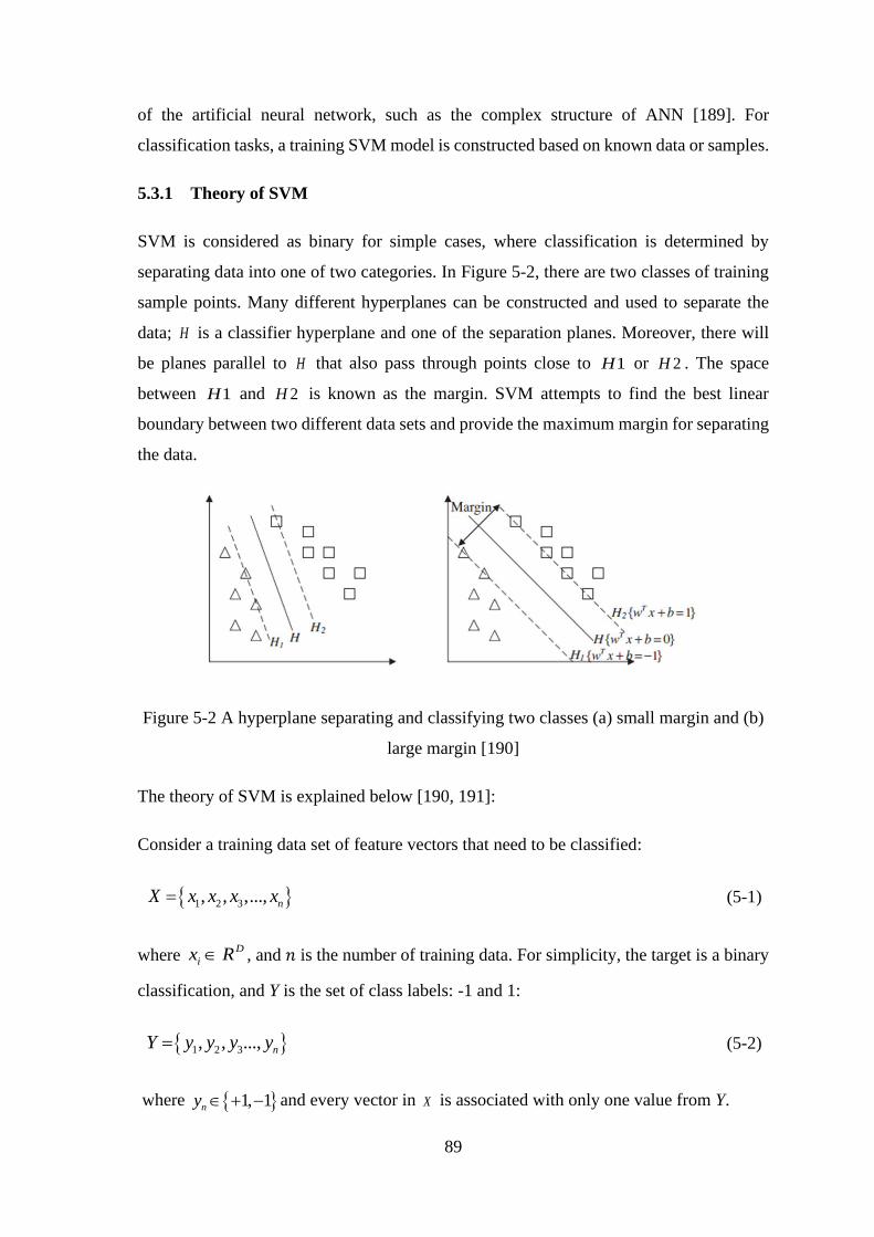
89

of the artificial neural network, such as the complex structure of ANN [189]. For

classification tasks, a training SVM model is constructed based on known data or samples.

5.3.1 Theory of SVM

SVM is considered as binary for simple cases, where classification is determined by

separating data into one of two categories. In Figure 5-2, there are two classes of training

sample points. Many different hyperplanes can be constructed and used to separate the

data; H is a classifier hyperplane and one of the separation planes. Moreover, there will

be planes parallel to H that also pass through points close to 1H or 2H . The space

between 1H and 2H is known as the margin. SVM attempts to find the best linear

boundary between two different data sets and provide the maximum margin for separating

the data.

Figure 5-2 A hyperplane separating and classifying two classes (a) small margin and (b)

large margin [190]

The theory of SVM is explained below [190, 191]:

Consider a training data set of feature vectors that need to be classified:

21 3, , ,..., nX x x x x= (5-1)

where D

ix R , and 𝑛 is the number of training data. For simplicity, the target is a binary

classification, and Y is the set of class labels: -1 and 1:

1 2 3, , ..., nY y y y y= (5-2)

where 1, 1ny + − and every vector in X is associated with only one value from Y.

90

The broad aim of SVM is to find the best hyperplane that will separate the training data,

which can be expressed via the following equation:

( ). 0, , T Dw x b where w R b R+ = (5-3)

where the vector Tw defines the weights, x is the input vector, and b is a constant. From

this, the classifier can be expressed as:

( )( ) . Ty f x sig w x b= = + (5-4)

In a real situation, the two classes can be separated by a margin with two hyperplanes (H1

and H2) as shown in Figure 5-2, The data points that lie closest to these hyperplanes are

called support vectors, and a suitable set of support vectors will uniquely define the

maximum margin between hyperplanes, giving the greatest separation between the planes

to avoid misclassification. In addition, to avoid having data points fall into the margin, the

data should satisfy the following constraints:

( )

( )

. 1 1

. 1 1

T

i

T

i

w x b when y

w x b when y

+ + = +

+ − = − (5-5)

Geometrically, the distance between 𝐻1 and 𝐻2 is 2

Tw , and the target is to maximize

the margin. To achieve this, the vector Tw needs to be minimized. In other words, the

combination of the constraints can be expressed as follows:

2

Tmin

w

( ). 1 0 T

iyi w x b i+ − (5-6)

In order to include a further elastic separating hyperplane for non-linear data, a slack

variable is introduced, and the corresponding constraint optimisation problem must be

minimized:

91

2

, ,

1

1

2

NT

w b z i

i

min w C =

+ (5-7)

From the previous formula, the constraints become:

𝑦𝑖(𝑤𝑇 . 𝑥𝑖) + 𝑏 ≥ 1 −𝑖 𝑖

and 𝑖 𝑖

≥ 0

(5-8)

where the training data ix is mapped into a higher-dimensional space in order to separate

it (which is easier than separating it in the original space), w is the weight vector, b is

bias, and is the slack variable.

To control the flexibility of the resulting SVM, a smoothing parameter c is used [192].

Equation 5-8 is referred to as a classical optimization problem. By using Lagrange

multipliers , 1,..., ,i i N = and using the Kuhn-Tucker formula from optimization theory,

the problem can be reduced to:

( ) ( )2

1 1

1, , .

2

N NT

i i i i

i i

L w b w C y w x b = =

= − + + (5-9)

To resolve Equation (5-9) the derivation of b with respect to w , and the derivation of L

with respect to all can be removed. Subsequently, the gradient of the Lagrangian

equation will consider the following condition:

1 1

, 0 N N

i i i i i

i i

w y x y = =

= = (5-10)

Coupling 5-9 and 5-10, together, a dual quadratic optimisation problem is obtained:

( )

1 1

1 .

2

N N

i i j i j i j

i ij

L y y x x = =

= − (5-11)

Subject to 1

0, 0 N

i i i

i

y =

= (5-12)

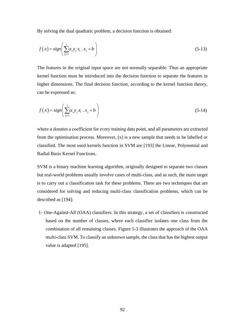
92

By solving the dual quadratic problem, a decision function is obtained:

( )

1

.l

i j i j

ij

f x sign y x x b=

= +

(5-13)

The features in the original input space are not normally separable. Thus an appropriate

kernel function must be introduced into the decision function to separate the features in

higher dimensions. The final decision function, according to the kernel function theory,

can be expressed as:

( )

1

.l

i j i j

ij

f x sign y x x b=

= +

(5-14)

where α donates a coefficient for every training data point, and all parameters are extracted

from the optimisation process. Moreover, (x) is a new sample that needs to be labelled or

classified. The most used kernels function in SVM are [193] the Linear, Polynomial and

Radial Basis Kernel Functions.

SVM is a binary machine learning algorithm, originally designed to separate two classes

but real-world problems usually involve cases of multi-class, and as such, the main target

is to carry out a classification task for these problems. There are two techniques that are

considered for solving and reducing multi-class classification problems, which can be

described as [194]:

1- One-Against-All (OAA) classifiers: In this strategy, a set of classifiers is constructed

based on the number of classes, where each classifier isolates one class from the

combination of all remaining classes. Figure 5-3 illustrates the approach of the OAA

multi-class SVM. To classify an unknown sample, the class that has the highest output

value is adapted [195].

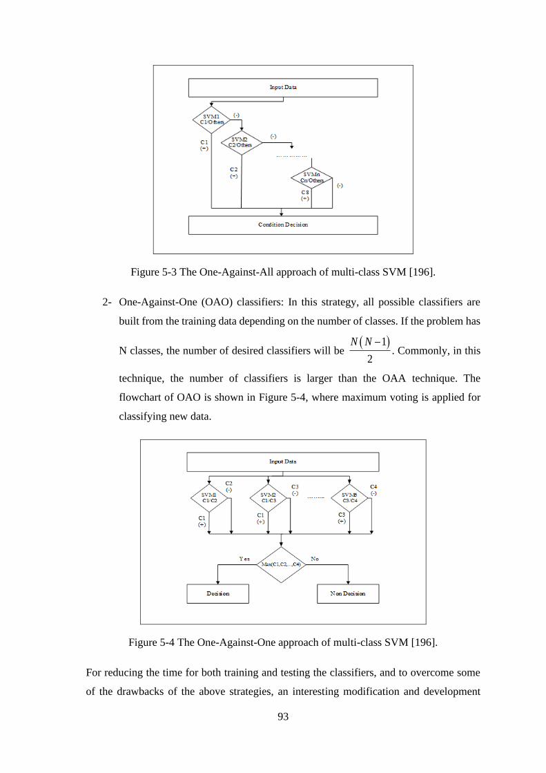
93

Figure 5-3 The One-Against-All approach of multi-class SVM [196].

2- One-Against-One (OAO) classifiers: In this strategy, all possible classifiers are

built from the training data depending on the number of classes. If the problem has

N classes, the number of desired classifiers will be ( )

2

1N N −. Commonly, in this

technique, the number of classifiers is larger than the OAA technique. The

flowchart of OAO is shown in Figure 5-4, where maximum voting is applied for

classifying new data.

Figure 5-4 The One-Against-One approach of multi-class SVM [196].

For reducing the time for both training and testing the classifiers, and to overcome some

of the drawbacks of the above strategies, an interesting modification and development

94

technique was introduced by Platt, et al., [197] which is an OAO-SVM based on the

Directed Acyclic Graph (DAG) method.

Figure 5-5 depicts the structure of the multi-class SVM with a Directed Acyclic Graph

approach and shows how it works with a three-class classification problem. The approach

has one classifier for every node. Testing or classifying new data involves starting at the

root node, where the pairwise decision is evaluated. The next move then depends on the

output value, where either the left or the right classifier will be applied in each succeeding

step until one of the leave nodes is reached, which characterizes the class label of the given

data.

1/3

21 3

1/2 2/3

Figure 5-5 SVM with a Directed Acyclic Graph for a multi-classification problem [198].

SVM used for CM has demonstrated good performance regarding fault diagnosis and is

very useful due to its generalisation ability compared with other methods such as ANNs.

Moreover, SVMs can learn from small data sets, which means that a SVM is an appropriate

method for practical cases where it is difficult to gather large data sets [188].

SVM is generally used for classifying the condition of a machine. In this context, selection

of the kernel function is vital as it strongly affects the accuracy of the results. Furthermore,

it is essential to obtain effective features to be utilised for constructing and training the

SVM model. Therefore, SVM is utilized with advanced signal analysis techniques where

meaningful features can be extracted to facilitate the distinction between different samples

and enhance the overall CM task.

Muralidharan et al. [11] used SVM for fault diagnosis of mono-block centrifugal pumps,

where they analysed the vibration signals for different pump conditions. These signals

95

were decomposed by a CW transform after which a number of transformation coefficient

features were extracted from all wavelets, and the distinguishing conditions were classified

by SVM. Qu [199] proposed a data processing algorithm for fault classification of the

degree of wear of slurry pump impellers, where the acquired vibration data was processed

using time and frequency domain features, selected on the basis of the sequential backward

selection technique, and the classification was then determined based on SVM, The results

indicated that the proposed method was capable of categorised different simulated faults

in an effective way.

5.4 Feature Extraction

Generally, feature extraction takes place before classification, where the main purpose of

extracting features is to map a set of measures that represent the original data set into a

new space where some specific aspects of the data will be more important for classification

decisions than others. Thus, the classification model can be simply constructed based on

certain agreed and important features [3].

Statistical parameters have been widely used in CM as diagnostic features to assess a

machine’s condition, where the extracted features are used to represent the raw signal by

minimizing the dimensions of the gathered datasets. The representative extracted features

hold the most important data components which can be used to easily classify the health

conditions of the machine. It is desirable to employ specific features for training and testing

the classification model [200]. Extracting and selecting relevant and meaningful features

from the acquired data is vital for obtaining an accurate classification model for CM.

In this research, statistical features are obtained from the current signal. These features are

used for building the classification, as well as for detecting and diagnosing the faults of

the pump. These features and their formulas are presented below [200] [201, 202]:

1. Root Mean Square (RMS): is the square root of the mean of the squared values

of samples, see Section 1.2.1.

2. Kurtosis: determines the shape of the data or signal, whether flat or spiky, see

Section 1.2.2.

3. The Crest factor: it is the ratio of the peak value to the RMS value, see Section

1.2.3.

96

4. Variance: is the average of the squares of the distance for each value from the

mean. The formula for variance is given by:

2

1var

( )n

i

i

x x

Xn

=

−

=

(5-15)

5. Entropy: can be used to describe the amount of information afforded by a

signal [203], and can be computed by this equation by:

2

1

( ) log ( )n

ent i i

i

X p x p x=

= (5-16)

where ( )ip x is the probability for the ith point of the signal.

6. Range: is the difference between the maximum and minimum signal point

values.

5.5 Key Findings

Machine learning can find non-linear patterns from the acquired data, and these

patterns can be used to a build model that can be utilised for classifying the health

condition of rotating machines. The classification model can be constructed based on

learning data and a machine learning algorithm, where the accuracy of such a model

depends on both of them. SVM is a robust machine learning technique for settling

nonlinear and high dimension data problems and has a good generalisation capability

compared with ANNs. The application of ML to CM is influenced by the size of the

data, and the feature extraction and selection. Thus, extracting and selecting relevant

and meaningful feature using data-driven techniques will contribute to establishing a

robust classifier, leading to accurate results for determining the condition of the

centrifugal pump.

97

Experimental Test Facility Setup and Fault

Simulation

This chapter presents the test facilities utilized in this research. The test rig components

are presented in details, which include the description and justification of measuring

instrumentation. Then it describes how pump faults were simulated. Finally, the chapter

describes the experimental procedure were used for obtaining the current signals from the

tests of different faulty cases.

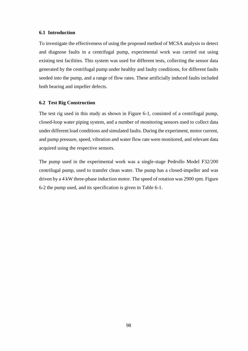
98

6.1 Introduction

To investigate the effectiveness of using the proposed method of MCSA analysis to detect

and diagnose faults in a centrifugal pump, experimental work was carried out using

existing test facilities. This system was used for different tests, collecting the sensor data

generated by the centrifugal pump under healthy and faulty conditions, for different faults

seeded into the pump, and a range of flow rates. These artificially induced faults included

both bearing and impeller defects.

6.2 Test Rig Construction

The test rig used in this study as shown in Figure 6-1, consisted of a centrifugal pump,

closed-loop water piping system, and a number of monitoring sensors used to collect data

under different load conditions and simulated faults. During the experiment, motor current,

and pump pressure, speed, vibration and water flow rate were monitored, and relevant data

acquired using the respective sensors.

The pump used in the experimental work was a single-stage Pedrollo Model F32/200

centrifugal pump, used to transfer clean water. The pump has a closed-impeller and was

driven by a 4 kW three-phase induction motor. The speed of rotation was 2900 rpm. Figure

6-2 the pump used, and its specification is given in Table 6-1.

99

Figure 6-1 The test-rig facility

Water tanks

Suction Discharge

Encoder

Centrifugal pump

100

Figure 6-2 The centrifugal pump used in this work (Pedrollo Model F32/200)

Table 6-1 Specification of the centrifugal pump

6.3 Test Rig Facility

To achieve the main objective of this study, a test facility is required for gathering data

and evaluating various data analysis techniques. There is such test rig available in the

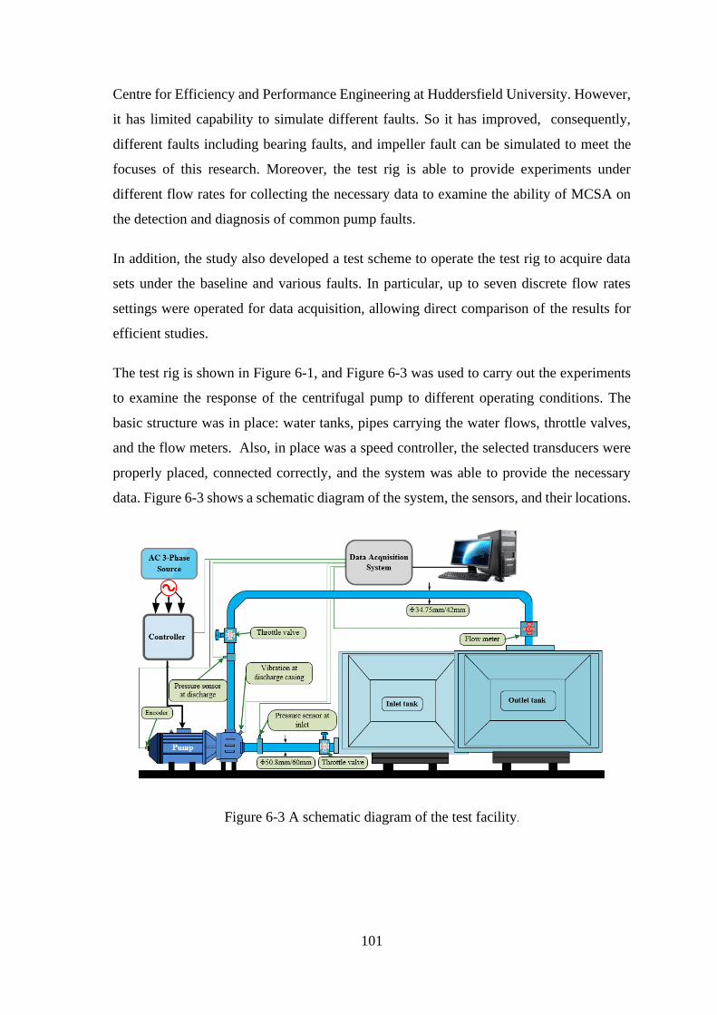
101

Centre for Efficiency and Performance Engineering at Huddersfield University. However,

it has limited capability to simulate different faults. So it has improved, consequently,

different faults including bearing faults, and impeller fault can be simulated to meet the

focuses of this research. Moreover, the test rig is able to provide experiments under

different flow rates for collecting the necessary data to examine the ability of MCSA on

the detection and diagnosis of common pump faults.

In addition, the study also developed a test scheme to operate the test rig to acquire data

sets under the baseline and various faults. In particular, up to seven discrete flow rates

settings were operated for data acquisition, allowing direct comparison of the results for

efficient studies.

The test rig is shown in Figure 6-1, and Figure 6-3 was used to carry out the experiments

to examine the response of the centrifugal pump to different operating conditions. The

basic structure was in place: water tanks, pipes carrying the water flows, throttle valves,

and the flow meters. Also, in place was a speed controller, the selected transducers were

properly placed, connected correctly, and the system was able to provide the necessary

data. Figure 6-3 shows a schematic diagram of the system, the sensors, and their locations.

Figure 6-3 A schematic diagram of the test facility.

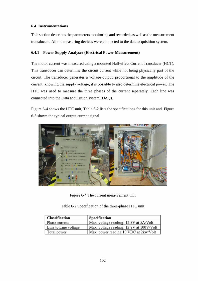
102

6.4 Instrumentations

This section describes the parameters monitoring and recorded, as well as the measurement

transducers. All the measuring devices were connected to the data acquisition system.

6.4.1 Power Supply Analyser (Electrical Power Measurement)

The motor current was measured using a mounted Hall-effect Current Transducer (HCT).

This transducer can determine the circuit current while not being physically part of the

circuit. The transducer generates a voltage output, proportional to the amplitude of the

current; knowing the supply voltage, it is possible to also determine electrical power. The

HTC was used to measure the three phases of the current separately. Each line was

connected into the Data acquisition system (DAQ).

Figure 6-4 shows the HTC unit, Table 6-2 lists the specifications for this unit and. Figure

6-5 shows the typical output current signal.

Figure 6-4 The current measurement unit

Table 6-2 Specification of the three-phase HTC unit

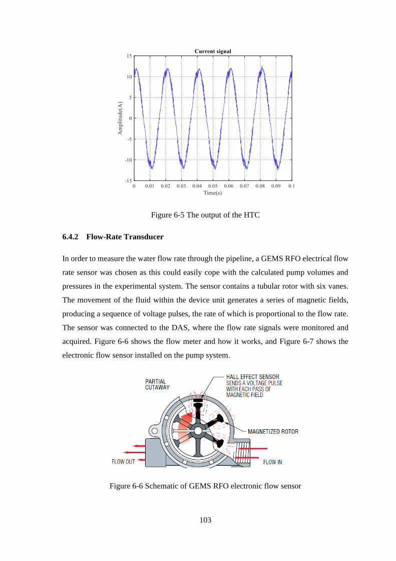
103

Figure 6-5 The output of the HTC

6.4.2 Flow-Rate Transducer

In order to measure the water flow rate through the pipeline, a GEMS RFO electrical flow

rate sensor was chosen as this could easily cope with the calculated pump volumes and

pressures in the experimental system. The sensor contains a tubular rotor with six vanes.

The movement of the fluid within the device unit generates a series of magnetic fields,

producing a sequence of voltage pulses, the rate of which is proportional to the flow rate.

The sensor was connected to the DAS, where the flow rate signals were monitored and

acquired. Figure 6-6 shows the flow meter and how it works, and Figure 6-7 shows the

electronic flow sensor installed on the pump system.

Figure 6-6 Schematic of GEMS RFO electronic flow sensor

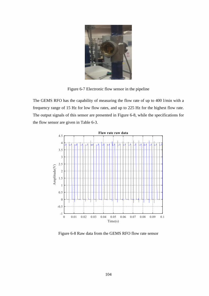
104

Figure 6-7 Electronic flow sensor in the pipeline

The GEMS RFO has the capability of measuring the flow rate of up to 400 l/min with a

frequency range of 15 Hz for low flow rates, and up to 225 Hz for the highest flow rate.

The output signals of this sensor are presented in Figure 6-8, while the specifications for

the flow sensor are given in Table 6-3.

Figure 6-8 Raw data from the GEMS RFO flow rate sensor

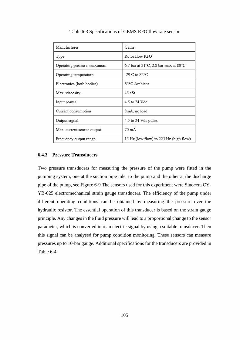
105

Table 6-3 Specifications of GEMS RFO flow rate sensor

6.4.3 Pressure Transducers

Two pressure transducers for measuring the pressure of the pump were fitted in the

pumping system, one at the suction pipe inlet to the pump and the other at the discharge

pipe of the pump, see Figure 6-9 The sensors used for this experiment were Sinocera CY-

YB-025 electromechanical strain gauge transducers. The efficiency of the pump under

different operating conditions can be obtained by measuring the pressure over the

hydraulic resistor. The essential operation of this transducer is based on the strain gauge

principle. Any changes in the fluid pressure will lead to a proportional change to the sensor

parameter, which is converted into an electric signal by using a suitable transducer. Then

this signal can be analysed for pump condition monitoring. These sensors can measure

pressures up to 10-bar gauge. Additional specifications for the transducers are provided in

Table 6-4.

106

Figure 6-9 Pressure transducers installed at the pump inlet and outlet

Table 6-4 Specifications of the pressure transducer

6.4.4 Speed Controller

For this test rig system, an Omron speed controller was used to control the pump speed.

Figure 6-10 shows the speed control unit and Table 6-5 device specifications.

107

Figure 6-10 Omron speed controller, external and internal views

Table 6-5 Speed controller specifications

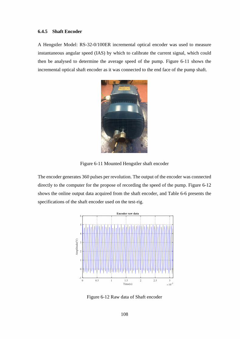
108

6.4.5 Shaft Encoder

A Hengstler Model: RS-32-0/100ER incremental optical encoder was used to measure

instantaneous angular speed (IAS) by which to calibrate the current signal, which could

then be analysed to determine the average speed of the pump. Figure 6-11 shows the

incremental optical shaft encoder as it was connected to the end face of the pump shaft.

Figure 6-11 Mounted Hengstler shaft encoder

The encoder generates 360 pulses per revolution. The output of the encoder was connected

directly to the computer for the propose of recording the speed of the pump. Figure 6-12

shows the online output data acquired from the shaft encoder, and Table 6-6 presents the

specifications of the shaft encoder used on the test-rig.

Figure 6-12 Raw data of Shaft encoder

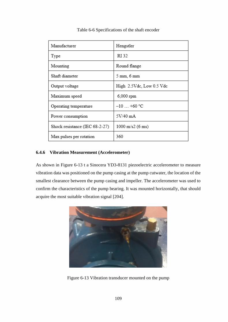
109

Table 6-6 Specifications of the shaft encoder

6.4.6 Vibration Measurement (Accelerometer)

As shown in Figure 6-13 t a Sinocera YD3-8131 piezoelectric accelerometer to measure

vibration data was positioned on the pump casing at the pump cutwater, the location of the

smallest clearance between the pump casing and impeller. The accelerometer was used to

confirm the characteristics of the pump bearing. It was mounted horizontally, that should

acquire the most suitable vibration signal [204].

Figure 6-13 Vibration transducer mounted on the pump

110

Figure 6-14 Output signal of the accelerometer

The accelerometer was used to measure vibration generated in the pump to provide data

to confirm the presence of the mechanical faults seeded into the pump, and to determine

the presence of expected fault frequencies corresponding to known bearing defects. The

given accelerometer has a frequency range of 10 Hz- 10 kHz, and an upper limit to the

acceleration range of 2000 ms-2. The specifications for the accelerometer are given Table

6-7.

Table 6-7 Specifications of the accelerometer

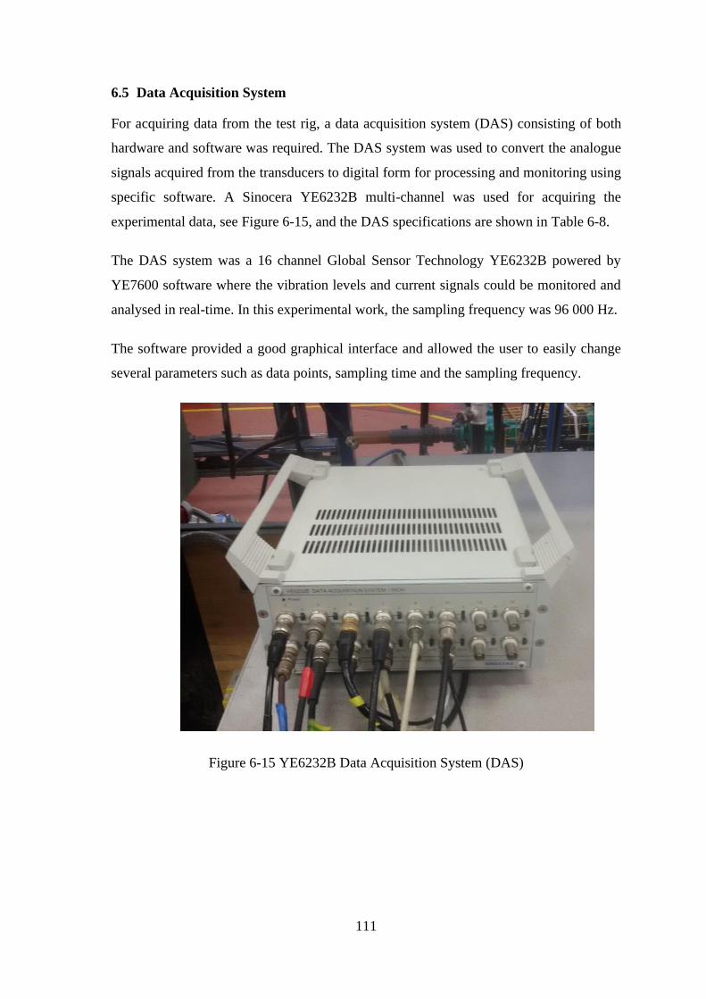
111

6.5 Data Acquisition System

For acquiring data from the test rig, a data acquisition system (DAS) consisting of both

hardware and software was required. The DAS system was used to convert the analogue

signals acquired from the transducers to digital form for processing and monitoring using

specific software. A Sinocera YE6232B multi-channel was used for acquiring the

experimental data, see Figure 6-15, and the DAS specifications are shown in Table 6-8.

The DAS system was a 16 channel Global Sensor Technology YE6232B powered by

YE7600 software where the vibration levels and current signals could be monitored and

analysed in real-time. In this experimental work, the sampling frequency was 96 000 Hz.

The software provided a good graphical interface and allowed the user to easily change

several parameters such as data points, sampling time and the sampling frequency.

Figure 6-15 YE6232B Data Acquisition System (DAS)

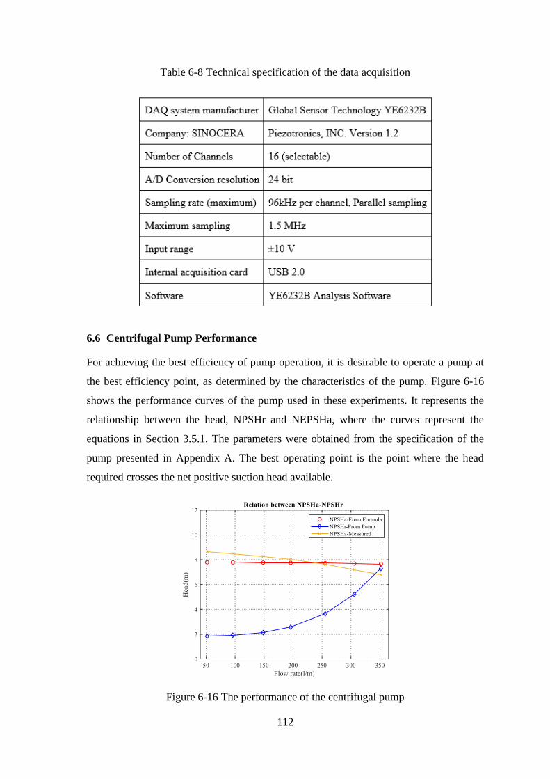
112

Table 6-8 Technical specification of the data acquisition

6.6 Centrifugal Pump Performance

For achieving the best efficiency of pump operation, it is desirable to operate a pump at

the best efficiency point, as determined by the characteristics of the pump. Figure 6-16

shows the performance curves of the pump used in these experiments. It represents the

relationship between the head, NPSHr and NEPSHa, where the curves represent the

equations in Section 3.5.1. The parameters were obtained from the specification of the

pump presented in Appendix A. The best operating point is the point where the head

required crosses the net positive suction head available.

Figure 6-16 The performance of the centrifugal pump

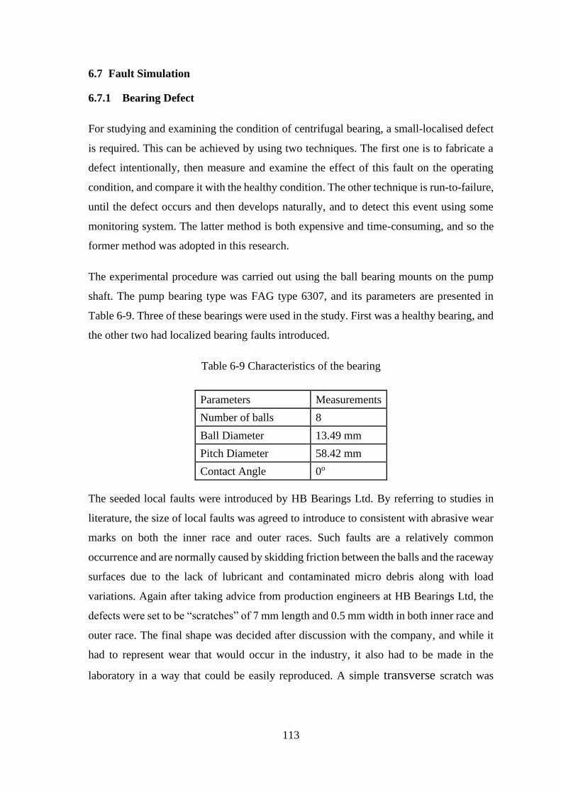
113

6.7 Fault Simulation

6.7.1 Bearing Defect

For studying and examining the condition of centrifugal bearing, a small-localised defect

is required. This can be achieved by using two techniques. The first one is to fabricate a

defect intentionally, then measure and examine the effect of this fault on the operating

condition, and compare it with the healthy condition. The other technique is run-to-failure,

until the defect occurs and then develops naturally, and to detect this event using some

monitoring system. The latter method is both expensive and time-consuming, and so the

former method was adopted in this research.

The experimental procedure was carried out using the ball bearing mounts on the pump

shaft. The pump bearing type was FAG type 6307, and its parameters are presented in

Table 6-9. Three of these bearings were used in the study. First was a healthy bearing, and

the other two had localized bearing faults introduced.

Table 6-9 Characteristics of the bearing

Parameters Measurements

Number of balls 8

Ball Diameter 13.49 mm

Pitch Diameter 58.42 mm

Contact Angle 0o

The seeded local faults were introduced by HB Bearings Ltd. By referring to studies in

literature, the size of local faults was agreed to introduce to consistent with abrasive wear

marks on both the inner race and outer races. Such faults are a relatively common

occurrence and are normally caused by skidding friction between the balls and the raceway

surfaces due to the lack of lubricant and contaminated micro debris along with load

variations. Again after taking advice from production engineers at HB Bearings Ltd, the

defects were set to be “scratches” of 7 mm length and 0.5 mm width in both inner race and

outer race. The final shape was decided after discussion with the company, and while it

had to represent wear that would occur in the industry, it also had to be made in the

laboratory in a way that could be easily reproduced. A simple transverse scratch was

114

finally decided on, as shown in Figure 6-17. The dimensions of the scratch were estimates

made of what could represent a real, in situ, fault.

(a)

(b)

Figure 6-17 (a) Inner race defect (b) Outer race defect

Figure 6-18 shows the relation between the pump head and corresponding flow for the

healthy pump, pump with inner race fault, and outer race fault. There is no significant

change in pump performance with bearing defects compared to the healthy condition.

Figure 6-18 Pump head vs Flow rate for (i) healthy pump (baseline), (ii) pump with inner

race fault and (iii) pump with outer race fault

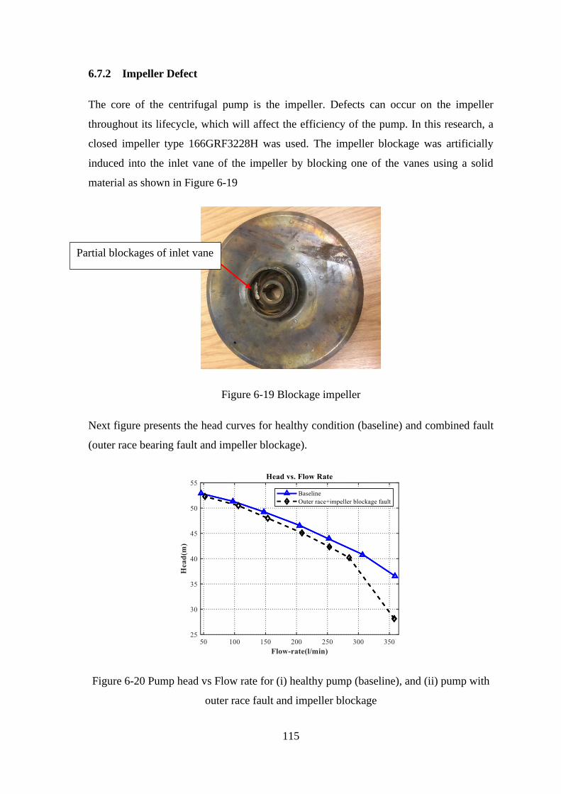
115

6.7.2 Impeller Defect

The core of the centrifugal pump is the impeller. Defects can occur on the impeller

throughout its lifecycle, which will affect the efficiency of the pump. In this research, a

closed impeller type 166GRF3228H was used. The impeller blockage was artificially

induced into the inlet vane of the impeller by blocking one of the vanes using a solid

material as shown in Figure 6-19

Figure 6-19 Blockage impeller

Next figure presents the head curves for healthy condition (baseline) and combined fault

(outer race bearing fault and impeller blockage).

Figure 6-20 Pump head vs Flow rate for (i) healthy pump (baseline), and (ii) pump with

outer race fault and impeller blockage

Partial blockages of inlet vane

116

Figure 6-20 shows that the combined defect produces a significant reduction in pump

performance compared by the healthy condition. This is what would be expected, as the

blockage impacts directly on the flow.

6.8 Experimental Procedure

In this study, various flow rates were investigated to simulate different conditions. The

normal condition (baseline/healthy) of the pump and three types of common faults were

investigated: the inner race bearing fault alone, the outer race bearing fault alone, and the

combined outer race bearing fault with impeller blockage.

For the experiment to be carried out under steady-state conditions, the pump was turned

on for half an hour before starting to collect data. Then the data were recorded for different

flow rates for durations of 40 seconds. The signals recorded were; motor current and

voltage, pump vibration and speed, pressure at inlet to pump and water flow rate. To assess

the influence of the faults on the performance of the pump, the signals were measured

under different flow rates, which were adjusted manually step by step using the throttling

valve in the discharge line. The flow rates were set to be 50, 100, 150 200, 250, 300 and

350 l/min. However, when set the flow rate, the accuracy was less than ± 5 l/ min, after

which the flow was constant.

The experimental procedures for the different tests can be summarised as follows:

• All tests were carried out at a fixed pump speed of 2900 rpm.

• The DAS recorded the current signals from the current transducer, as described in

Section 6.4.1.

• The DAS was linked to the computer for online monitoring of the system.

• The pumping system was operated for half an hour before recording the data in

order to achieve steady-state conditions for pump operation.

• The test procedure was carried out in the following order: (a) healthy pump (b)

bearing with inner race fault (c) bearing with outer race fault (d) a combined fault

(outer race fault + blocked impeller ).

• To ensure the accuracy of the acquired data, each test was repeated three times

under the same conditions.

117

• All data sets were recorded for a period of 40 seconds to provide sufficient data

samples for understanding the characteristics of motor current for enhancing the

diagnostic techniques.

• The obtained current signals were processed and analysed by a MATLAB program

written by the author.

6.9 Key Findings

This chapter presents the developed test rig in detail, all the equipment used for simulating

and monitoring the centrifugal pump healthy and under different faults are described,

including all electrical and mechanical parts. The chapter also presented the specifications

of the instruments and transducers. Finally, the fault simulations and test procedures have

been explained.

118

Detection and Diagnosis of Centrifugal Pump

Faults using Conventional Current Signal Analysis

Technique

This chapter evaluates the performances of conventional MCSA regarding fault detection

under different pump flow rates. The gathered data were analysed in both the time domain

and frequency domain. The healthy condition of the centrifugal pump was adopted as the

baseline condition. Also, a comprehensive comparison with the other defect data sets has

been made. The results showed that the motor current signatures can provide a solid basis

for identifying the given pump faults.

119

7.1 Introduction

The current signals were gathered under four pump conditions: healthy pump, inner race

fault, outer race fault, and combined fault (impeller blockage and outer race bearing fault).

All four conditions were investigated under different flow rates: 50, 100, 150, 200, 250,

300, and 350 l/m. All experiments were conducted at pump speed 2900 rpm, with a

sampling rate of 96 kHz, see Section 6.7 for more details.

7.2 Time Domain Analysis (waveform)

It is the primary method for describing the collection data such as electrical signal and, as

a function of time. Generally, time domain analysis looks at data over a period of time.

Figure 7-1 shows electrical current waveforms recorded for the centrifugal pump for

different flow rates, for the healthy and three faulty conditions described. The current

signal for a baseline, healthy pump is presented as a blue line, and the three induced faults

are shown as: inner race - red line, outer race - pink line, and combined faults of outer race

and impeller blockage - black line. Here the flow rates were 350, 300, and 250 l/min.

120

Figure 7-1 Time-domain waveforms for baseline, inner race, outer race and combined

fault (outer race and impeller blockage) under different flow rates

From Figure 7-1, the amplitude of the current signal increases with the increase in the flow

rate, though this is not easily discernible as the signals have an amplitude modulation,

especially at low flow rates. At this stage of analysis of the current data, it is hard to detect

changes in the current signatures between the different fault cases, as the amplitude of the

current signals is nearly the same for all the cases at a given flow rate. However, a small

change was noticed between the combined fault and baseline condition.

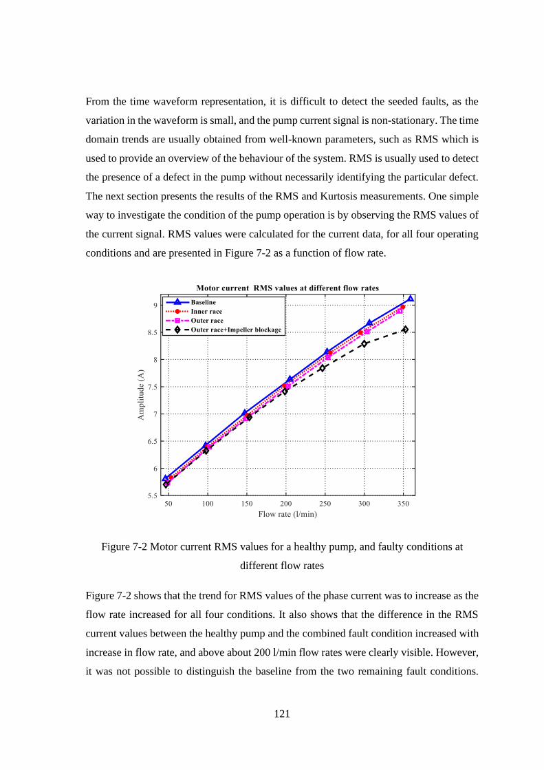
121

From the time waveform representation, it is difficult to detect the seeded faults, as the

variation in the waveform is small, and the pump current signal is non-stationary. The time

domain trends are usually obtained from well-known parameters, such as RMS which is

used to provide an overview of the behaviour of the system. RMS is usually used to detect

the presence of a defect in the pump without necessarily identifying the particular defect.

The next section presents the results of the RMS and Kurtosis measurements. One simple

way to investigate the condition of the pump operation is by observing the RMS values of

the current signal. RMS values were calculated for the current data, for all four operating

conditions and are presented in Figure 7-2 as a function of flow rate.

Figure 7-2 Motor current RMS values for a healthy pump, and faulty conditions at

different flow rates

Figure 7-2 shows that the trend for RMS values of the phase current was to increase as the

flow rate increased for all four conditions. It also shows that the difference in the RMS

current values between the healthy pump and the combined fault condition increased with

increase in flow rate, and above about 200 l/min flow rates were clearly visible. However,

it was not possible to distinguish the baseline from the two remaining fault conditions.

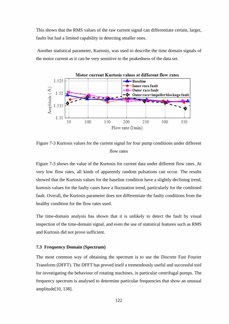
122

This shows that the RMS values of the raw current signal can differentiate certain, larger,

faults but had a limited capability in detecting smaller ones.

Another statistical parameter, Kurtosis, was used to describe the time domain signals of

the motor current as it can be very sensitive to the peakedness of the data set.

Figure 7-3 Kurtosis values for the current signal for four pump conditions under different

flow rates

Figure 7-3 shows the value of the Kurtosis for current data under different flow rates. At

very low flow rates, all kinds of apparently random pulsations can occur. The results

showed that the Kurtosis values for the baseline condition have a slightly declining trend,

kurtosis values for the faulty cases have a fluctuation trend, particularly for the combined

fault. Overall, the Kurtosis parameter does not differentiate the faulty conditions from the

healthy condition for the flow rates used.

The time-domain analysis has shown that it is unlikely to detect the fault by visual

inspection of the time-domain signal, and even the use of statistical features such as RMS

and Kurtosis did not prove sufficient.

7.3 Frequency Domain (Spectrum)

The most common way of obtaining the spectrum is to use the Discrete Fast Fourier

Transform (DFFT). The DFFT has proved itself a tremendously useful and successful tool

for investigating the behaviour of rotating machines, in particular centrifugal pumps. The

frequency spectrum is analysed to determine particular frequencies that show an unusual

amplitude[10, 138].

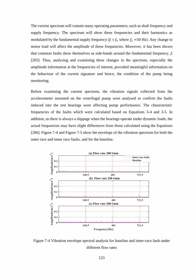
123

The current spectrum will contain many operating parameters, such as shaft frequency and

supply frequency. The spectrum will show these frequencies and their harmonics as

modulated by the fundamental supply frequency (fi ± fs, where 𝑓𝑠 =50 Hz). Any change in

motor load will affect the amplitude of these frequencies. Moreover, it has been shown

that common faults show themselves as side-bands around the fundamental frequency, fi

[205]. Thus, analysing and examining these changes in the spectrum, especially the

amplitude information at the frequencies of interest, provided meaningful information on

the behaviour of the current signature and hence, the condition of the pump being

monitoring.

Before examining the current spectrum, the vibration signals collected from the

accelerometer mounted on the centrifugal pump were analysed to confirm the faults

induced into the test bearings were affecting pump performance. The characteristic

frequencies of the faults which were calculated based on Equations 3-4 and 3-5. In

addition, as there is always a slippage when the bearings operate under dynamic loads, the

actual frequencies may have slight differences from those calculated using the Equations

[206]. Figure 7-4 and Figure 7-5 show the envelope of the vibration spectrum for both the

outer race and inner race faults, and for the baseline.

Figure 7-4 Vibration envelope spectral analysis for baseline and inner-race fault under


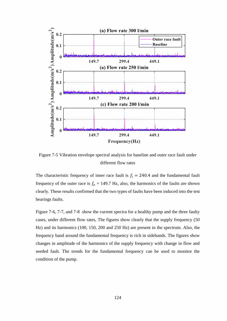
124

Figure 7-5 Vibration envelope spectral analysis for baseline and outer race fault under


The characteristic frequency of inner race fault is 𝑓𝑖 = 240.4 and the fundamental fault

frequency of the outer race is 𝑓𝑜 = 149.7 Hz, also, the harmonics of the faults are shown

clearly. These results confirmed that the two types of faults have been induced into the test

bearings faults.

Figure 7-6, 7-7, and 7-8 show the current spectra for a healthy pump and the three faulty

cases, under different flow rates, The figures show clearly that the supply frequency (50

Hz) and its harmonics (100, 150, 200 and 250 Hz) are present in the spectrum. Also, the

frequency band around the fundamental frequency is rich in sidebands. The figures show

changes in amplitude of the harmonics of the supply frequency with change in flow and

seeded fault. The trends for the fundamental frequency can be used to monitor the

condition of the pump.

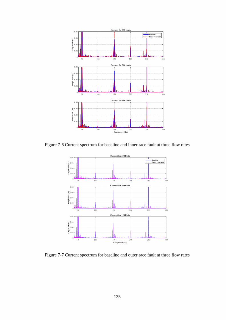
125

Figure 7-6 Current spectrum for baseline and inner race fault at three flow rates

Figure 7-7 Current spectrum for baseline and outer race fault at three flow rates

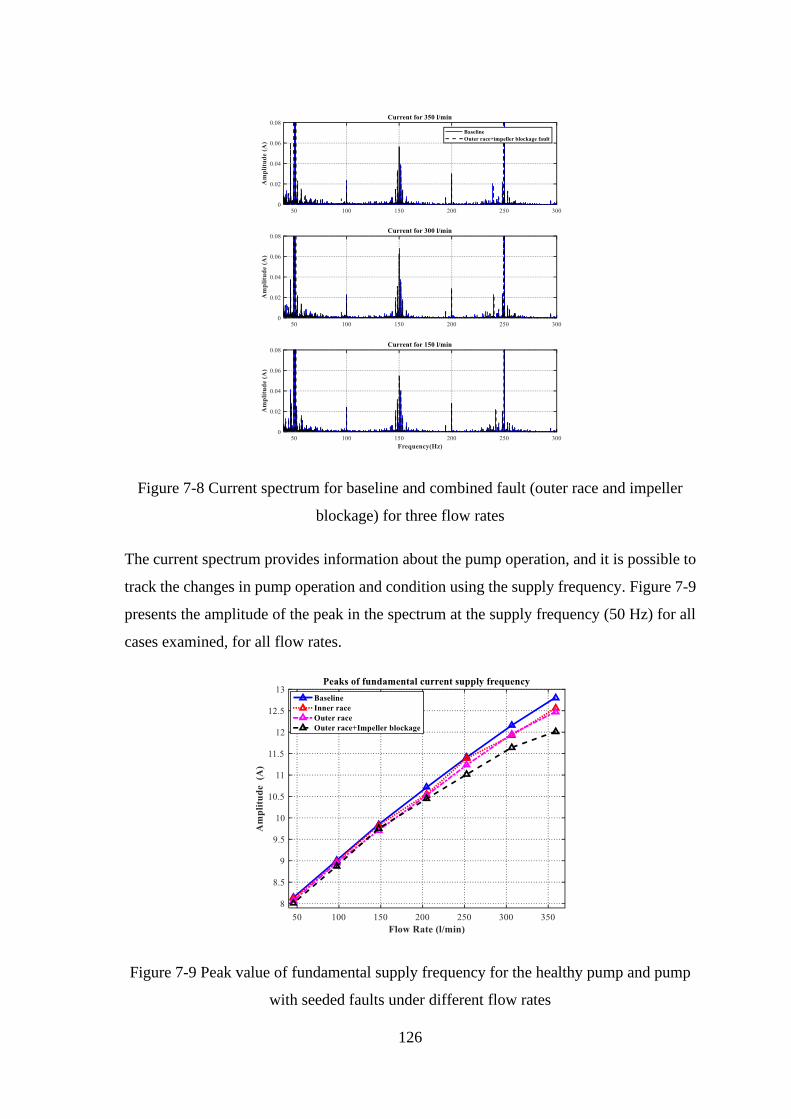
126

Figure 7-8 Current spectrum for baseline and combined fault (outer race and impeller

blockage) for three flow rates

The current spectrum provides information about the pump operation, and it is possible to

track the changes in pump operation and condition using the supply frequency. Figure 7-9

presents the amplitude of the peak in the spectrum at the supply frequency (50 Hz) for all

cases examined, for all flow rates.

Figure 7-9 Peak value of fundamental supply frequency for the healthy pump and pump

with seeded faults under different flow rates

127

It can be seen that the amplitude of current at the supply frequency increased with

increasing flow rate. In the figure, the same trend can be seen for all four conditions, the

amplitude of the motor current increased monotonically with flow rate. The figure also

shows that the healthy case can be distinguished from the faulty cases, certainly at flow

rates higher than 250 l/min, but it is difficult to separate the different conditions for lower

flow rates.

At this stage, the bearing fault frequencies could not be directly determined from the

current spectrum, and further investigation was carried out based on envelope analysis, to

identify these bearing fault frequencies. For envelope analysis, a bandpass filter is required

to eliminate the low-frequency noise, then the signal was rectified, and after that, the

envelope of the spectrum was obtained, from which the fault frequency components could

be detected. The envelope analysis was performed for the current signals for all conditions

for three flow rates. Figure 7-10 shows the results of the envelope analysis of the current

signals.

Figure 7-10 Envelope spectrum of current signal for baseline and inner race fault under


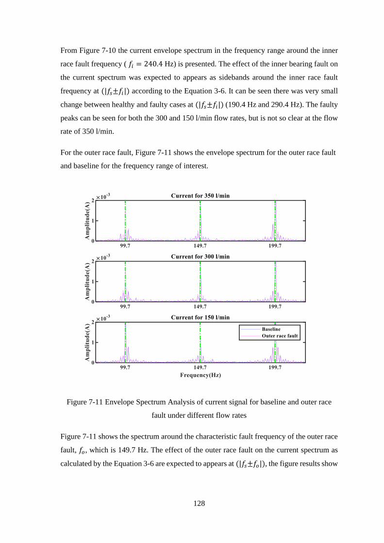
128

From Figure 7-10 the current envelope spectrum in the frequency range around the inner

race fault frequency ( 𝑓𝑖 = 240.4 Hz) is presented. The effect of the inner bearing fault on

the current spectrum was expected to appears as sidebands around the inner race fault

frequency at (|𝑓𝑠±𝑓𝑖|) according to the Equation 3-6. It can be seen there was very small

change between healthy and faulty cases at (|𝑓𝑠±𝑓𝑖|) (190.4 Hz and 290.4 Hz). The faulty

peaks can be seen for both the 300 and 150 l/min flow rates, but is not so clear at the flow

rate of 350 l/min.

For the outer race fault, Figure 7-11 shows the envelope spectrum for the outer race fault

and baseline for the frequency range of interest.

Figure 7-11 Envelope Spectrum Analysis of current signal for baseline and outer race

fault under different flow rates

Figure 7-11 shows the spectrum around the characteristic fault frequency of the outer race

fault, 𝑓𝑜, which is 149.7 Hz. The effect of the outer race fault on the current spectrum as

calculated by the Equation 3-6 are expected to appears at (|𝑓𝑠±𝑓𝑜|), the figure results show

129

a peak at the characteristic fault frequency of the outer race 𝑓𝑜 ± 𝑓𝑠, for all flow rates, while

the peaks at 𝑓𝑜 are small than baseline.

However, the modulating components of the bearing faults had very small amplitudes and

were masked by the background noise. It would be difficult to detect the peaks belonging

to the outer and inner race faults from the current spectrum. Thus, an advanced signal

processing technique such as a data-driven technique is required for analysing the current

signals to determine the presence of mechanical defects.

7.4 Key Findings

This chapter has presented an overview of the use of motor current signals for evaluating

the condition of the centrifugal pump for fault detection and diagnosis.

Time-domain analysis and frequency domain analysis has carried out for tracking the

change of the current signal caused by the induced faults. Although the slight change of

the RMS values which has a monotonic increase in amplitude with flow rate, it is unlikely

to detect the faults in the centrifugal pump.

Moreover, from the results obtained using current spectrum and the envelope analysis

showed that bearing faults have very small amplitudes and were masked by the

background noise, it can be concluded that it is still not adequate to identify the pump

faults. As the current signals are affected by complicated nonlinear processes such as the

fluctuations in the flow rate. Further investigation will be carried out based on the data-

driven techniques such as EMD and ITD for analyses and examine the use of current

signals for monitoring the performance of centrifugal pumps.

130

Empirical Mode Decomposition of Motor

Current Signal for Centrifugal Pump Diagnostics

This chapter offers a data-driven method of extracting characteristics from the motor

current signature to detect and diagnose centrifugal pump faults. Specifically, the

procedure utilizes the unique advantages of Empirical mode decomposition for

decomposing the current signal, and then uses envelope analysis for the demodulation of

the decomposed signal. This allows the extraction of features from the current signal to

assess the condition of the pump. The results show that the combination of EMD and

envelope analysis can be an effective method for detecting the seeded pump faults.

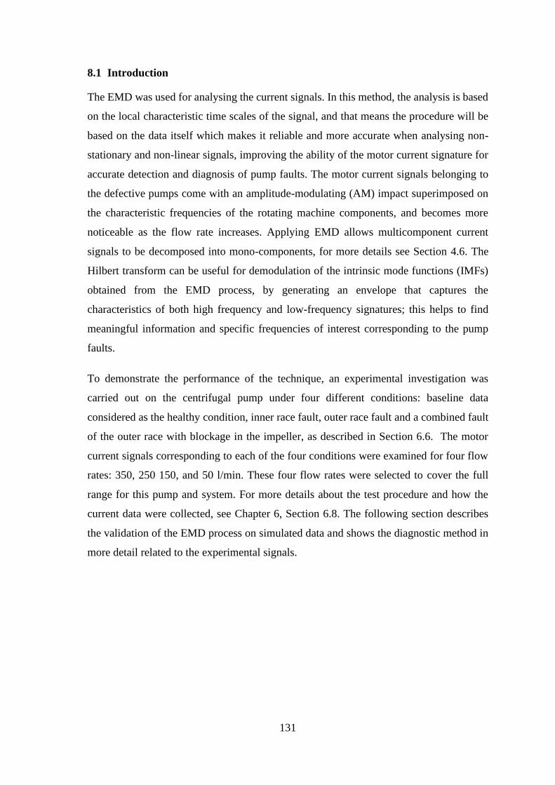
131

8.1 Introduction

The EMD was used for analysing the current signals. In this method, the analysis is based

on the local characteristic time scales of the signal, and that means the procedure will be

based on the data itself which makes it reliable and more accurate when analysing non-

stationary and non-linear signals, improving the ability of the motor current signature for

accurate detection and diagnosis of pump faults. The motor current signals belonging to

the defective pumps come with an amplitude-modulating (AM) impact superimposed on

the characteristic frequencies of the rotating machine components, and becomes more

noticeable as the flow rate increases. Applying EMD allows multicomponent current

signals to be decomposed into mono-components, for more details see Section 4.6. The

Hilbert transform can be useful for demodulation of the intrinsic mode functions (IMFs)

obtained from the EMD process, by generating an envelope that captures the

characteristics of both high frequency and low-frequency signatures; this helps to find

meaningful information and specific frequencies of interest corresponding to the pump

faults.

To demonstrate the performance of the technique, an experimental investigation was

carried out on the centrifugal pump under four different conditions: baseline data

considered as the healthy condition, inner race fault, outer race fault and a combined fault

of the outer race with blockage in the impeller, as described in Section 6.6. The motor

current signals corresponding to each of the four conditions were examined for four flow

rates: 350, 250 150, and 50 l/min. These four flow rates were selected to cover the full

range for this pump and system. For more details about the test procedure and how the

current data were collected, see Chapter 6, Section 6.8. The following section describes

the validation of the EMD process on simulated data and shows the diagnostic method in

more detail related to the experimental signals.

132

8.2 The Performance of EMD on Numerical Simulation Signal

To validate the efficiency and performance of the EMD method for analyzing a non-

stationary signal, a simulated signal with noise-contaminated AM is considered as

follows[125]:

𝑥 = 𝐴𝐿 cos(2πfst − fL − αL) + 𝐴𝑐 cos(2πfst + αc) + 𝐴𝑈 cos(2πfst + fU − αU) + 𝐴𝑛 𝑛(𝑡)

where fs=50.0 Hz, fL = fU=48.5 Hz corresponds to the supply frequency and shaft

rotational frequency. The carrier signal, Ac, has an amplitude of unity, and αc, αL , αx are

random phases from a uniform distribution between 0 and 2𝜋.

The modulating signal has an amplitude 𝐴𝐿 =𝐴𝑈 =0.01, and the noise has a uniform

distribution between 0 and 2𝜋. The signal includes random noise 𝑛(𝑡) which is from a

normal distribution denoted as N~ N(µ=0, 𝜎2=1), where µ is the mean and 𝜎2 is the

variance; the noise amplitude, 𝐴𝑛 = 0.1.

This simulated signal is analogous to recorded current data where the carrier signal comes

with much higher amplitude than other components. The simulated signal, see Figure

8.1(a), was sampled at a frequency of 2048 Hz. Figure 8-1(a) and (b), shows the signal 𝑥

in the time domain, also, it contains the same essential features of the AM of the measured

signal shown in Figure 4-1. The frequency-domain spectrum corresponding to Figure

8.1(a) is shown in Figure 8-1 (b). This simulation will assist in establishing the analytic

characteristics of the measured signals. The simulated signal was decomposed by EMD

technique into IMF components, see Figure 8.2. It is clear that the first IMF contains the

highest frequency components and, subsequently, the other IMFs contain lower

frequencies.

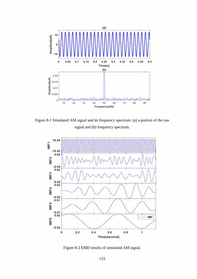
133

Figure 8-1 Simulated AM signal and its frequency spectrum: (a) a portion of the raw

signal and (b) frequency spectrum.

Figure 8-2 EMD results of simulated AM signal.

134

8.3 The Performance of EMD on Experimental Current Signal

The current signals of different cases with a varying range of flow rates were decomposed

using the EMD techniques, as shown in figures Figure 8-3 to Figure 8-6 only the six IMFs

and their envelopes are presented for all cases with flow rate at 250 l/min. It is obvious

that the profiles of the distinct IMF components have some differences, it is clear that the

first IMF component has more fluctuations and modulation characteristics.

Figure 8-3 EMD decomposition results of Baseline at 250 l/min

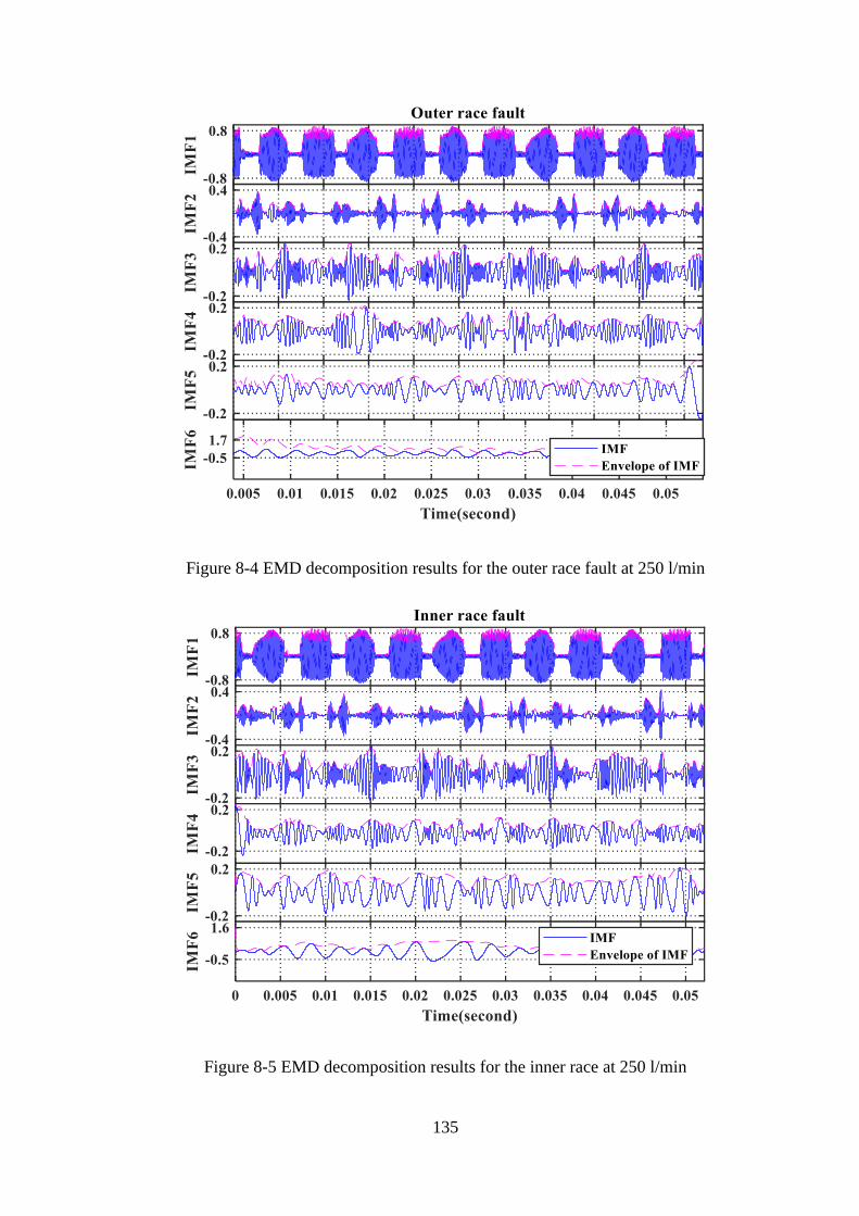
135

Figure 8-4 EMD decomposition results for the outer race fault at 250 l/min

Figure 8-5 EMD decomposition results for the inner race at 250 l/min

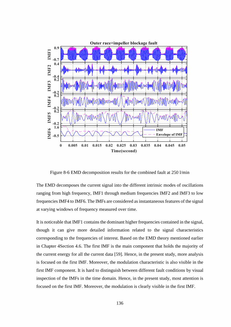
136

Figure 8-6 EMD decomposition results for the combined fault at 250 l/min

The EMD decomposes the current signal into the different intrinsic modes of oscillations

ranging from high frequency, IMF1 through medium frequencies IMF2 and IMF3 to low

frequencies IMF4 to IMF6. The IMFs are considered as instantaneous features of the signal

at varying windows of frequency measured over time.

It is noticeable that IMF1 contains the dominant higher frequencies contained in the signal,

though it can give more detailed information related to the signal characteristics

corresponding to the frequencies of interest. Based on the EMD theory mentioned earlier

in Chapter 4Section 4.6. The first IMF is the main component that holds the majority of

the current energy for all the current data [59]. Hence, in the present study, more analysis

is focused on the first IMF. Moreover, the modulation characteristic is also visible in the

first IMF component. It is hard to distinguish between different fault conditions by visual

inspection of the IMFs in the time domain. Hence, in the present study, most attention is

focused on the first IMF. Moreover, the modulation is clearly visible in the first IMF.

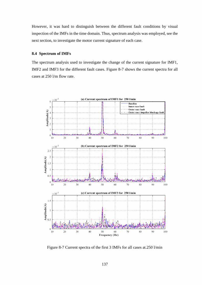
137

However, it was hard to distinguish between the different fault conditions by visual

inspection of the IMFs in the time domain. Thus, spectrum analysis was employed, see the

next section, to investigate the motor current signature of each case.

8.4 Spectrum of IMFs

The spectrum analysis used to investigate the change of the current signature for IMF1,

IMF2 and IMF3 for the different fault cases. Figure 8-7 shows the current spectra for all

cases at 250 l/m flow rate.

Figure 8-7 Current spectra of the first 3 IMFs for all cases at.250 l/min

138

Figure 8-7 in (a), (b) and (c) shows the spectrum analysis of the first, second and the third

IMFs, respectively. In the first IMF, the fundamental frequency can be seen at 50 Hz, with

a higher amplitude compared to the results obtained from IMF2 and IMF3. Figure 8-8

presents comparisons of the peak amplitude values of the supply frequency for the healthy

pump and faulty condition.

Figure 8-8 Peak values at fs from the current spectrums of IMF1 and IMF2

Figure 8-8 presents the peak values of the first and second IMFs, it is obvious that the fs

values of IMF2 show more fluctuations and a greater spread than IMF1. However, there

is no clear trend in either of IMF1 or IMF2. Based on these results, it is not possible to

separate the healthy condition from the seeded faults using the characteristic extracted

from the spectrums of the IMFs. However, the frequency peaks caused by the defect may

be hidden beneath the frequencies from the rotating parts such as the shaft. Thus, envelope

spectral analysis was applied to determine the characteristic frequencies from the IMF

components of the modulated signal.

8.5 Envelope Spectrum of IMFs

The motor current signal has inherent modulation effects generated from the variation of

load on the centrifugal pump. The IMF components have an amplitude modulation (AM)

effect due to the raw current signal for the various operating conditions of the pump. Thus,

envelope analysis of the IMFs was performed in order to obtain envelope spectra from

which the mechanical fault might be diagnosed. The Fourier transform of the envelope

signal of the first three IMFs was computed as these contain the higher frequencies of the

signal that may provide some important diagnostic features.

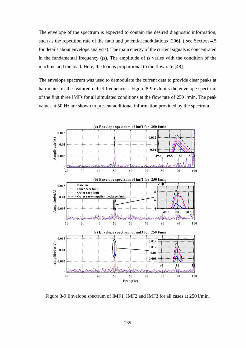
139

The envelope of the spectrum is expected to contain the desired diagnostic information,

such as the repetition rate of the fault and potential modulations [206], ( see Section 4.5

for details about envelope analysis). The main energy of the current signals is concentrated

in the fundamental frequency (fs). The amplitude of fs varies with the condition of the

machine and the load. Here, the load is proportional to the flow rate [48].

The envelope spectrum was used to demodulate the current data to provide clear peaks at

harmonics of the featured defect frequencies. Figure 8-9 exhibits the envelope spectrum

of the first three IMFs for all simulated conditions at the flow rate of 250 l/min. The peak

values at 50 Hz are shown to present additional information provided by the spectrum.

Figure 8-9 Envelope spectrum of IMF1, IMF2 and IMF3 for all cases at 250 l/min.

140

In Figure 8-9 (a) it is noticeable that the spectral peaks at the fundamental frequency fs of

50 Hz for the IMF1 have different amplitudes and show a clear separation between all four

the cases, as seen in the magnified graph. This feature provides a good indication of the

pump’s condition, while the second and third IMFs show the same signal amplitudes for

the inner race fault and the outer race fault, see Figure 8-9 (b-c). It is obvious that using

IMF2 and IMF3 for the separation of these simulated cases would not be possible.

Figure 8-10 shows the peak values of the fundamental frequency in IMF1 and IMF2 for

all cases.

Figure 8-10 Peak value of fs from the envelope spectrum for IMF1 and IMF2

From the Figure 8-10, it is clear that the inner and outer race faults have nearly the same

peak values for IMF2 in most of the operation conditions, while the peak values for IMF1

provide good results that distinguish between the baseline and the simulated conditions,

note the same trend for the magnitudes to decrease as flow increased is observed in all the

cases. Thus, the first IMF was adopted for detecting the pump faults, where more

information related to the current signals is found.

8.6 Key Findings

In this chapter, a centrifugal pump detection method has been applied based on the EMD

and Hilbert transform. The EMD characteristics, which include noise reduction and

nonlinear signature enhancement combined with envelope analysis, provide more accurate

and convincing results. The current signals were decomposed into a number of IMF’s that

include the fault signatures. The results show that the EMD analysis combined with

141

envelope spectra of the current signature is proved to be effective in detecting a seeded

fault condition in a centrifugal pump under several flow rates, and it is extremely effective

than the other conventional analysis method used in this study.

142

Intrinsic Time Scale Decomposition for Fault

Detection and Diagnosis of Centrifugal Pump

This chapter provides a data-driven technique to detect and diagnose defects in the

centrifugal pump. The method comprises decomposing the current signal by applying an

advanced data analysis technique such as intrinsic time scale decomposition (ITD) and

investigates its capability for extracting information hidden in the current data.

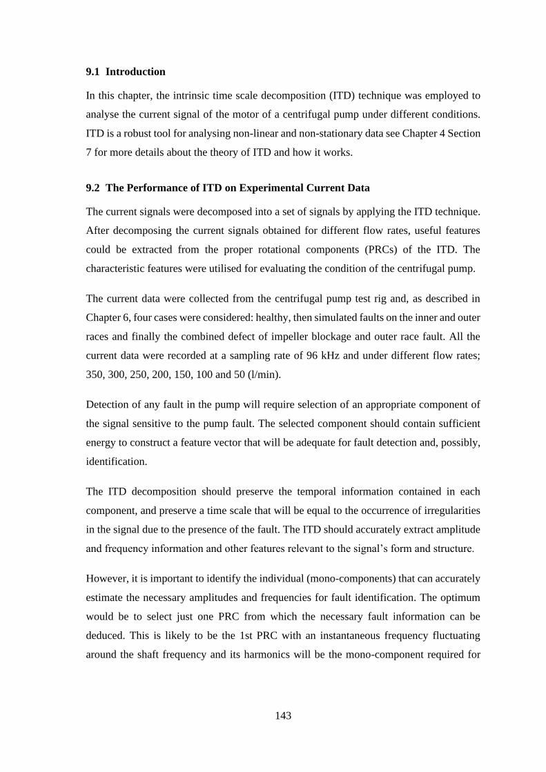
143

9.1 Introduction

In this chapter, the intrinsic time scale decomposition (ITD) technique was employed to

analyse the current signal of the motor of a centrifugal pump under different conditions.

ITD is a robust tool for analysing non-linear and non-stationary data see Chapter 4 Section

7 for more details about the theory of ITD and how it works.

9.2 The Performance of ITD on Experimental Current Data

The current signals were decomposed into a set of signals by applying the ITD technique.

After decomposing the current signals obtained for different flow rates, useful features

could be extracted from the proper rotational components (PRCs) of the ITD. The

characteristic features were utilised for evaluating the condition of the centrifugal pump.

The current data were collected from the centrifugal pump test rig and, as described in

Chapter 6, four cases were considered: healthy, then simulated faults on the inner and outer

races and finally the combined defect of impeller blockage and outer race fault. All the

current data were recorded at a sampling rate of 96 kHz and under different flow rates;

350, 300, 250, 200, 150, 100 and 50 (l/min).

Detection of any fault in the pump will require selection of an appropriate component of

the signal sensitive to the pump fault. The selected component should contain sufficient

energy to construct a feature vector that will be adequate for fault detection and, possibly,

identification.

The ITD decomposition should preserve the temporal information contained in each

component, and preserve a time scale that will be equal to the occurrence of irregularities

in the signal due to the presence of the fault. The ITD should accurately extract amplitude

and frequency information and other features relevant to the signal’s form and structure.

However, it is important to identify the individual (mono-components) that can accurately

estimate the necessary amplitudes and frequencies for fault identification. The optimum

would be to select just one PRC from which the necessary fault information can be

deduced. This is likely to be the 1st PRC with an instantaneous frequency fluctuating

around the shaft frequency and its harmonics will be the mono-component required for

144

additional analysis. Thus, here the author will investigate whether just the 1st PRC will be

sufficient for fault detection and identification.

Figure 9-1 ITD decomposition result for the healthy pump at 350 l/min.

Figure 9-2 ITD decomposition results for inner race bearing fault at 350 l/min.

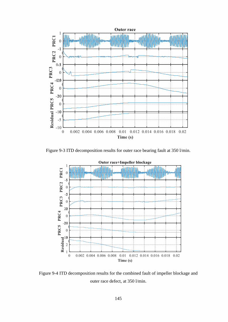
145

Figure 9-3 ITD decomposition results for outer race bearing fault at 350 l/min.

Figure 9-4 ITD decomposition results for the combined fault of impeller blockage and

outer race defect, at 350 l/min.

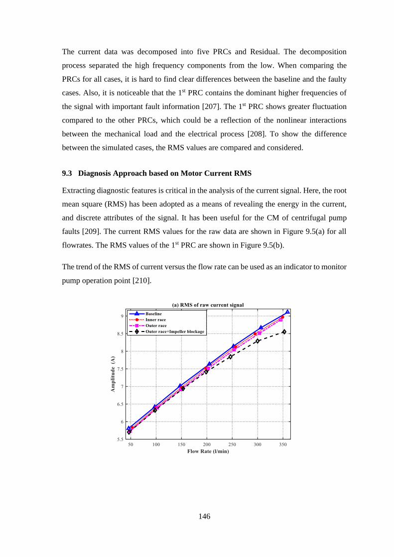
146

The current data was decomposed into five PRCs and Residual. The decomposition

process separated the high frequency components from the low. When comparing the

PRCs for all cases, it is hard to find clear differences between the baseline and the faulty

cases. Also, it is noticeable that the 1st PRC contains the dominant higher frequencies of

the signal with important fault information [207]. The 1st PRC shows greater fluctuation

compared to the other PRCs, which could be a reflection of the nonlinear interactions

between the mechanical load and the electrical process [208]. To show the difference

between the simulated cases, the RMS values are compared and considered.

9.3 Diagnosis Approach based on Motor Current RMS

Extracting diagnostic features is critical in the analysis of the current signal. Here, the root

mean square (RMS) has been adopted as a means of revealing the energy in the current,

and discrete attributes of the signal. It has been useful for the CM of centrifugal pump

faults [209]. The current RMS values for the raw data are shown in Figure 9.5(a) for all

flowrates. The RMS values of the 1st PRC are shown in Figure 9.5(b).

The trend of the RMS of current versus the flow rate can be used as an indicator to monitor

pump operation point [210].

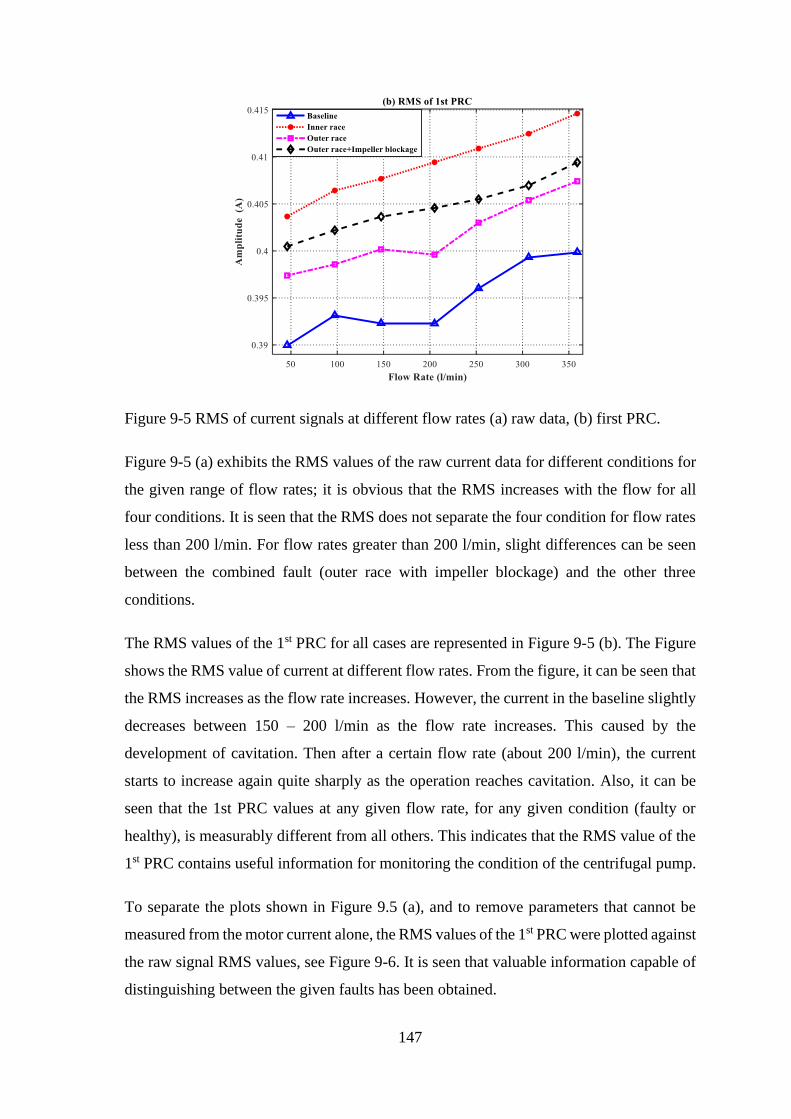
147

Figure 9-5 RMS of current signals at different flow rates (a) raw data, (b) first PRC.

Figure 9-5 (a) exhibits the RMS values of the raw current data for different conditions for

the given range of flow rates; it is obvious that the RMS increases with the flow for all

four conditions. It is seen that the RMS does not separate the four condition for flow rates

less than 200 l/min. For flow rates greater than 200 l/min, slight differences can be seen

between the combined fault (outer race with impeller blockage) and the other three

conditions.

The RMS values of the 1st PRC for all cases are represented in Figure 9-5 (b). The Figure

shows the RMS value of current at different flow rates. From the figure, it can be seen that

the RMS increases as the flow rate increases. However, the current in the baseline slightly

decreases between 150 – 200 l/min as the flow rate increases. This caused by the

development of cavitation. Then after a certain flow rate (about 200 l/min), the current

starts to increase again quite sharply as the operation reaches cavitation. Also, it can be

seen that the 1st PRC values at any given flow rate, for any given condition (faulty or

healthy), is measurably different from all others. This indicates that the RMS value of the

1st PRC contains useful information for monitoring the condition of the centrifugal pump.

To separate the plots shown in Figure 9.5 (a), and to remove parameters that cannot be

measured from the motor current alone, the RMS values of the 1st PRC were plotted against

the raw signal RMS values, see Figure 9-6. It is seen that valuable information capable of

distinguishing between the given faults has been obtained.

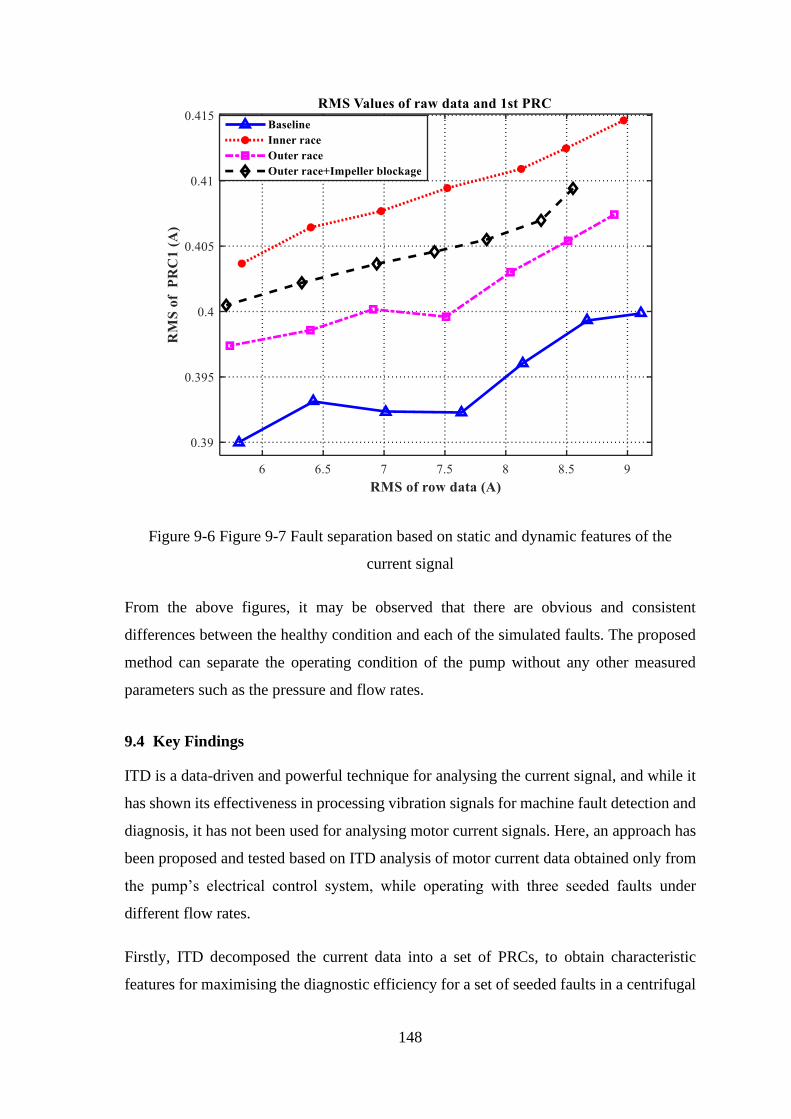
148

Figure 9-6 Figure 9-7 Fault separation based on static and dynamic features of the

current signal

From the above figures, it may be observed that there are obvious and consistent

differences between the healthy condition and each of the simulated faults. The proposed

method can separate the operating condition of the pump without any other measured

parameters such as the pressure and flow rates.

9.4 Key Findings

ITD is a data-driven and powerful technique for analysing the current signal, and while it

has shown its effectiveness in processing vibration signals for machine fault detection and

diagnosis, it has not been used for analysing motor current signals. Here, an approach has

been proposed and tested based on ITD analysis of motor current data obtained only from

the pump’s electrical control system, while operating with three seeded faults under

different flow rates.

Firstly, ITD decomposed the current data into a set of PRCs, to obtain characteristic

features for maximising the diagnostic efficiency for a set of seeded faults in a centrifugal

149

pump. The RMS of the motor current and the 1st PRC was employed as a useful feature

for describing the energy of the current signal. The results have demonstrated that the 1st

PRC extracted by ITD can adequately represent the motor operation. Also, a new feature

parameter is proposed that combined the RMS of the raw signal and RMS of the 1st PRC.

This has two advantages, firstly it shows a clearer separation among the different pump

conditions, at a given flow rate, and secondly, it is in terms of motor current parameters

only, it does not require, for example, pipe flow rate. Consequently, this proposed

approach performs effectively for detecting common pump faults under a wide range of

pressure.

150

Support Vector Machine for Enhance

Detection and Diagnosis of Centrifugal Pump Faults

This chapter discusses a proposed method for classifying the three faults seeded into a

centrifugal pump, based on current signals. A support vector machine (SVM) was

constructed and employed using intrinsic time-scale decomposition (ITD) features, which

were extracted from the current data for different fault cases and a range of flow rates.

This chapter assesses the capability of the method for centrifugal pump fault detection and

diagnosis. Also, the performance of envelope analysis, empirical mode decomposition

(EMD), and discrete wavelet transform (DWT) based features were investigated and

compared to ITD. The results demonstrate that the analysis method based on SVM and

ITD work efficiently for detection and diagnosis of the seeded defects in the centrifugal

pump. This diagnostic approach will enhance the condition monitoring of centrifugal

pumps.

151

10.1 Introduction

In this research, SVM was applied to classify the faults seeded into a centrifugal pump.

SVM was adopted due to the advantages it offers, such as having a generalization

capability and good classification performance [211]. SVM has the advantage that it can

cope with analysing large amounts of data that vary considerably, and data with a high

number of dimensions [212]. The principle of SVM is dependent on statistical learning

concepts and is generally considered to be very effective for finding an optimal solution

for classification problems. It is a robust machine learning technique that is appropriate

for machine fault diagnosis [213]. Hence, a multi-class SVM was applied to features

extracted from different signal processing techniques: ITD, envelope analysis, EMD, and

DWT. The next section explains the diagnostic approach to the centrifugal pump faults.

10.2 Centrifugal Pump Diagnostic Approach based on SVM

In this approach, the current data of a centrifugal pump are investigated for all four cases:

baseline, inner race fault, outer race fault, and the combined fault impeller blockage and

outer race bearing fault. Figure 10-1 presents a flowchart of the proposed diagnostic

approach based on SVM for centrifugal pump faults.

The diagnostic approach has three main processing stages. The process starts with the

current signals being acquired from the centrifugal pump test rig (see Section 6.8). In the

second stage, the current signals are analysed to extract statistical features to be used for

the classification task. These features are: Mean, RMS, Crest factor Kurtosis, Entropy,

Variance, and Range, (for more details about their formulas see Section 5.4), then in the

last stage, the SVM algorithm was employed for generating the classifier, which was used

to detect and diagnose the particular fault determining the condition of the pump.

152

Figure 10-1 An adaptive diagnostic approach for a centrifugal pump based on data

analysis and SVM.

10.3 SVM classifier based on ITD features

The current signals for each fault condition were analysed by ITD then the envelope

analysis method was applied to the signals. After that, the statistical features (Mean, RMS,

Crest factor Kurtosis, Entropy, Variance, and Range) were extracted from the first of the

proper rotation components (PRCs) that contains substantial information concerning the

current signal and used to generate the data sets.

153

For each case, the calculation of the seven features was obtained from 20 segments of the

current signal for each of seven flow rates. Then data sets were combined together, in

which the data corresponding to each of the four cases were distributed as 140 feature

vectors for each case. As shown in Table 10-1. The dataset is split into two data sets; a

training set (50%) and a testing set (50%). Each set contained the same number of cases,

which were randomly selected, the training set was used for classifier construction and the

test set for testing the model.

Table 10-1 Data set of statistical features (experimental data)

Fault

Number Fault condition

batch

size Training set Test set

1 Baseline 140 70 70

2 Inner race fault 140 70 70

3 Outer race fault 140 70 70

4 Outer race fault with

impeller blockage 140 70 70

The multi-SVM classifier was constructed using the MATLAB’s built-in function

‘fitcecoc’, which required the training data set as input arguments, where each row of this

matrix was given a class name that corresponded to the type of fault. Table 10-2 presents

the class designation number and the class name. It should also be noted that the kernel

function RBF was used to train the SVM classifier, that function was used because it is

has been shown to be better than other kernel functions such as the polynomial kernel, as

the hyperparameters are fewer than in other functions [189].

Table 10-2 Multiclass SVM class names

Class number Class label

1 Baseline

2 Inner race fault

3 Outer race fault

4 Outer race fault with blockage impeller

154

The constructed multiclass SVM classifier was then tested on the testing data set, where

the class label was unseen by the classifier. The accuracy of SVM classification was

computed using the standard formula for accuracy rate:

𝐴𝐶 =𝑛𝑢𝑚𝑏𝑒𝑟 𝑜𝑓 𝑐𝑜𝑟𝑟𝑒𝑐𝑡𝑙𝑦 𝑐𝑙𝑎𝑠𝑠𝑖𝑓𝑖𝑒𝑑 𝑠𝑎𝑚𝑝𝑙𝑒𝑠

𝑡𝑜𝑡𝑎𝑙 𝑛𝑢𝑚𝑏𝑒𝑟 𝑜𝑓 𝑠𝑎𝑚𝑝𝑙𝑒𝑠 𝑖𝑛 𝑑𝑎𝑡𝑎𝑠𝑒𝑡× 100 10-1

A confusion matrix that conveniently presents comparable information was used to

evaluate the SVM performance. The accuracy of results obtained from the classification

of testing data is presented in Figure 10-2.

Figure 10-2 Confusion matrix of multi-class SVM based on ITD features

Figure 10-2 shows the percentage of correct and incorrect classifications, that the classifier

produced from the test data according to their corresponding class label (machine

condition). The correct rate of the classification achieved across all cases was 99.6%,

giving a mis-classification of just 0.4%. The classifier was 100% accurate classifying all

155

cases of baseline (healthy pump), inner race fault and outer race fault, while the compound

fault had just one mis-classified.

Figure 10-3 shows the classification results in more detail, cases appear on blue trace are

correctly classified, whilst, only single misclassified case (shifted from the blue trace) is

the combined fault (outer race fault impeller blockage).

Figure 10-3 Multi-class SVM classification results using ITD features

10.4 SVM classifier based on EMD features

The current signals of each of the four conditions were analysed using EMD, the envelope

signals obtained, and statistical features (Mean, RMS, Crest factor Kurtosis, Entropy,

Variance, and Range), were extracted from the first IMF that contains most of the

information in the current signal, and using these features to generate the data sets. For

each fault case, the calculated statistical features were, again, obtained from 20

segmentations of the current signal for each of the seven flow rates. Then the data sets

were combined, in which the data corresponding to the fault cases were distributed as 140

feature vectors for each fault case.

The same procedure was carried out for dividing the dataset into training and testing sets,

and constructing the multi-SVM classifier. The confusion matrix, including the accuracy

rate of using EMD features is presented in Figure 10-4.

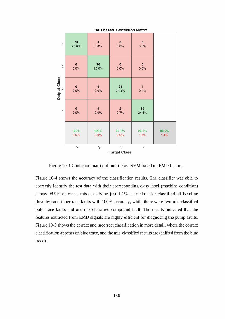
156

Figure 10-4 Confusion matrix of multi-class SVM based on EMD features

Figure 10-4 shows the accuracy of the classification results. The classifier was able to

correctly identify the test data with their corresponding class label (machine condition)

across 98.9% of cases, mis-classifying just 1.1%. The classifier classified all baseline

(healthy) and inner race faults with 100% accuracy, while there were two mis-classified

outer race faults and one mis-classified compound fault. The results indicated that the

features extracted from EMD signals are highly efficient for diagnosing the pump faults.

Figure 10-5 shows the correct and incorrect classification in more detail, where the correct

classification appears on blue trace, and the mis-classified results are (shifted from the blue

trace).

157

Figure 10-5 Multi-class SVM classification results using EMD features

10.5 SVM classifier based on DWT features:

The DWT is an implementation of the wavelet transform using discrete sets of the wavelet

scales. The application of DWT is faster than CWT with fewer parameters, and has a good

time and frequency resolutions [214]. The given signal is decomposed into low-pass

approximation coefficient and high-pass detailed coefficients, and then on the next levels,

only the approximation coefficients are decomposed into low-pass approximations while

the high-pass details are kept. Then the reconstruction signal is obtained through the

inverse wavelet transform of the detail coefficients [215].

The current signals for all the experimental conditions were analysed by DWT. The signal

was decomposed into six levels, then envelope analysis was applied to the reconstructed

signals, after that the same statistical features as listed above were extracted from 20

segmentations of each level of DWT results for each of the seven flow rates. When the

data sets were combined together, there are 140 feature vectors for each fault case.

The same procedure was carried out for dividing the dataset into training and testing sets,

and constructing the SVM classifier. The confusion matrix for showing the accuracy rate

obtained using DWT features is presented in Figure 10-6.

158

Figure 10-6 SVM Confusion matrix of multi-class SVM based on DWT features

The classifier classified all baseline (healthy) conditions correctly. There were two inner

race faults, ten outer race faults and seven compound faults mis-classified. The overall

accuracy rate was 93.2%.

Figure 10-7 shows the correct and incorrect classification based on DWT features in more

detail.

159

Figure 10-7 Multi-class SVM classification results using DWT features

10.6 SVM classifier based on Envelope features:

In this method, envelope analysis was applied to the current signals, after that the same

statistical features stated previously were extracted. Data sets were generated and using

these features from 20 segments of each envelope and for the seven flow rates. Then the

data sets were combined to provide 140 feature vectors for each fault case.

The same procedure as described above, was carried out for dividing the dataset into

training and testing sets, and constructing the multi-SVM classifier. The confusion matrix,

including the accuracy rate using envelope features is presented in Figure 10-8.

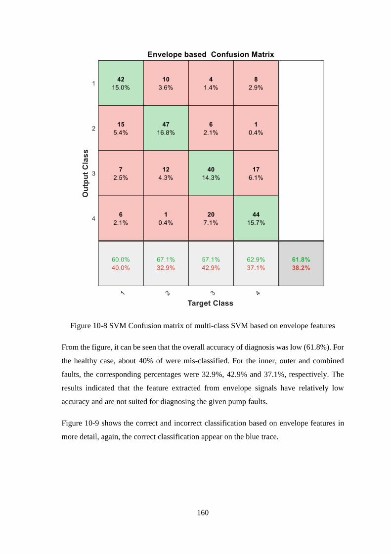
160

Figure 10-8 SVM Confusion matrix of multi-class SVM based on envelope features

From the figure, it can be seen that the overall accuracy of diagnosis was low (61.8%). For

the healthy case, about 40% of were mis-classified. For the inner, outer and combined

faults, the corresponding percentages were 32.9%, 42.9% and 37.1%, respectively. The

results indicated that the feature extracted from envelope signals have relatively low

accuracy and are not suited for diagnosing the given pump faults.

Figure 10-9 shows the correct and incorrect classification based on envelope features in

more detail, again, the correct classification appear on the blue trace.

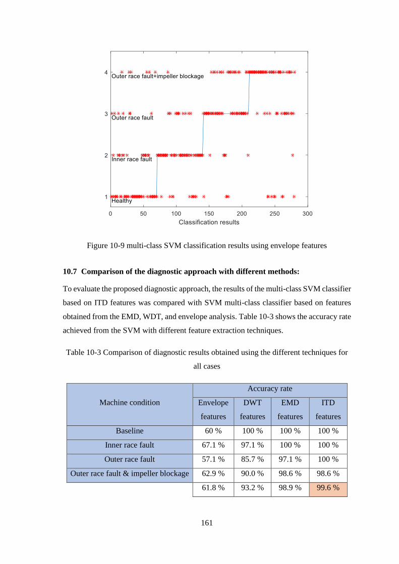
161

Figure 10-9 multi-class SVM classification results using envelope features

10.7 Comparison of the diagnostic approach with different methods:

To evaluate the proposed diagnostic approach, the results of the multi-class SVM classifier

based on ITD features was compared with SVM multi-class classifier based on features

obtained from the EMD, WDT, and envelope analysis. Table 10-3 shows the accuracy rate

achieved from the SVM with different feature extraction techniques.

Table 10-3 Comparison of diagnostic results obtained using the different techniques for

all cases

Machine condition

Accuracy rate

Envelope

features

DWT

features

EMD

features

ITD

features

Baseline 60 % 100 % 100 % 100 %

Inner race fault 67.1 % 97.1 % 100 % 100 %

Outer race fault 57.1 % 85.7 % 97.1 % 100 %

Outer race fault & impeller blockage 62.9 % 90.0 % 98.6 % 98.6 %

61.8 % 93.2 % 98.9 % 99.6 %

162

From Table 10.3, it can be seen that the classifier SVM based on ITD features provides

the best diagnostic information, for classification of the pump faults considered. The ITD

features are marginally better than EMD because of the better diagnosis of the outer race

fault (100% compared to 97.1%). However, a comparison of proportions showed no

significant difference overall between the results obtained from ITD and EMD features.

Also, ITD was significantly better at the 5% confidence level than DWT, mainly because

of the lower score of the DWT on the outer race fault. ITD was very much better at

diagnosis then the Envelope features at the 1% confidence level. Here a simple two-tailed

difference of proportions test was used.

The classification rates for the different methods tested are presented in Figure 10-10. By

examining the results of the table, it can be stated that utilizing ITD features for fault

diagnosis can significantly enhance the prediction accuracy of SVM compared to the

envelope, DWT and EMD. To compare the performance of the SVM classifier based on

ITD features with other studies from literature, a further comparison is presented in Table

10-4.

Figure 10-10 Comparison between different feature extraction techniques

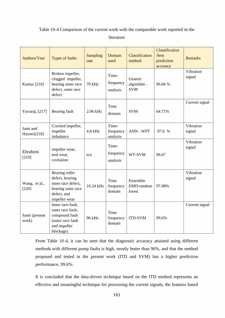
163

Table 10-4 Comparison of the current work with the comparable work reported in the

literature

Authors/Year Types of faults Sampling

rate

Domain

used

Classification

method

Classification

/best

prediction

accuracy

Remarks

Kumar [216]

Broken impeller,

clogged impeller,

bearing inner race

defect, outer race

defect

70 kHz

Time-

frequency

analysis

Genetic

algorithm -

SVM

96.66 %

Vibration

signal

Yuvaraj, [217] Bearing fault 2.06 kHz

Time

domain SVM 64.71%

Current signal

Jami and

Haynes[218]

Cracked impeller,

impeller

imbalance

4.8 kHz

Time-

frequency

analysis

ANN - WPT 97.6 %

Vibration

signal

Ebrahimi

[219]

impeller wear,

seal wear,

cavitation

n/a

Time-

frequency

analysis

WT-SVM 96.67

Vibration

signal

Wang, et al.,

[220]

Bearing roller

defect, bearing

inner race defect,

bearing outer race

defect, and

impeller wear

10.24 kHz

Time

frequency

domain

Ensemble

EMD-random

forest

97.08%

Vibration

signal

Sami (present

work)

Inner race fault,

outer race fault,

compound fault

(outer race fault

and impeller

blockage)

96 kHz

Time

frequency

domain

ITD-SVM 99.6%

Current signal

From Table 10-4, it can be seen that the diagnostic accuracy attained using different

methods with different pump faults is high, mostly better than 96%, and that the method

proposed and tested in the present work (ITD and SVM) has a higher prediction

performance, 99.6%.

It is concluded that the data-driven technique based on the ITD method represents an

effective and meaningful technique for processing the current signals, the features based

164

on ITD provide a good basis for describing the signature of the current signals. The

diagnostic approach based on ITD with SVM is very effective for classifying the simulated

faults of a centrifugal pump.

10.8 Key Findings

In this chapter, an intelligent diagnostic approach was proposed based on a data-driven

and machine learning technique for extracting meaningful features and distinguishing

between seeded faults. Remarkably high classification accuracy was achieved when the

SVM classifier was applied to ITD features, it shows the effectiveness of ITD in the task

of extracting informative features from the motor current signals. ITD based features

outperform envelope and DWT.

The results showed that the diagnostic approach (SVM and ITD) performed effectively,

enhanced the monitoring of the pump operation under different flow rates, thereby

demonstrating that it is capable of detecting and distinguishing between the given faults

based on their motor current signatures. Comparison of these with published results show

that SVM with ITD is effective as all other available techniques known to the author for

diagnosing pump faults.

165

Conclusions and Suggestions for Future

Work

This chapter summarises the main findings of this study, and provides an overview of its

major accomplishments. Additionally, a summary of the contributions of this research to

knowledge is presented. Finally, suggestions for possible future work on the CM of

centrifugal pumps are provided.

166

11.1 Review of the Aims, Objectives and Achievements

The main objective of this study was to produce a platform using advanced ML paradigms

capable of analysing the motor current signals of centrifugal pumps to detect developing

faults and produce an accurate diagnosis, to improve CM performance. A comprehensive

investigation, extracting fault features from current signals was carried out by using a

variety of motor current analysis techniques. For fault detection and identification, a

diagnostic approach based on data-driven methods, such as ITD and EMD, resulted in a

machine learning technique being adopted for this research programme. Advanced MCSA

techniques have been used to improve the diagnostic methods for three specific centrifugal

pump defects under a wide range of flow rates.

In this section, the achievements of this thesis are reviewed corresponding with the

research Objectives listed in Section 5.1. The objectives of this research have been fulfilled

as follows:

Objective 1. To review CM methods and maintenance strategies and explain the most

common techniques used for fault detection of centrifugal pumps.

Achievement: A comprehensive review of CM was presented to evaluate the techniques

most frequently used for monitoring rotating machines. These techniques were discussed

in Chapter 2; maintenance strategies and some essential concepts were considered in

Sections 2.3 and 2.4. It has been demonstrated that motor current analysis is a reliable

technique for detecting and diagnosing machine faults. This provided motivation for

investigating accurate and reliable monitoring techniques to achieve a more sensitive and

more accurate monitoring technique.

Objective 2. To refine the existing test facility and use it for monitoring the condition of

a centrifugal pump with different simulated pump faults under various flow rates.

Achievement: The existing facilities, suitably adapted, were used for investigating the

condition of the centrifugal pump under different operating conditions. A full description

and explanation of this test rig is presented in Chapter 6. The experimental tests were

performed on a healthy centrifugal pump and pump with three common faults seeded into

it. During the tests, several parameters were monitored and recorded, including flow rate,

167

vibration and suction pressure, to assess the pump condition. Motor current data were

gathered for the healthy and simulated fault conditions under various flow rates.

Objective 3. To examine the ability of motor current data obtained from the electrical

control system for detecting various mechanical faults of the pump by examining the

current signature using various signal process techniques.

Achievement 3: A comprehensive review has been presented in Section 2.6.4, to assess

the MCSA as a means of detecting and diagnosing faults in rotating machines. Also, some

theoretical background is presented to aid understanding of the characteristics of the

current data when the pump operates under different conditions and different loads. In

Section 3.8, the behaviour of the motor current is explained when changes in the load

torque resulted from change of working conditions, such as due to a mechanical defect,

will require corresponding modifications of the motor torque to maintain the desired pump

speed. This review demonstrated that the MSCA is reliable and accurate for fault detection

and diagnosis, and it can be employed in an effective means of monitoring the health of a

centrifugal.

Objective 4. To explore the current signal under different operating conditions using

conventional data analysis methods to identify and obtain the most critical fault defining

feature, that will be used for comparison with those obtained from the data-driven

techniques.

Achievement 4: Conventional signal processing techniques according to the time and

frequency domain were applied to detect and diagnose the simulated pump faults. In

Chapter 7, it is shown that the given mechanical faults lead to a rise in the amplitude of

the current signals, also shown are some AM effects. However, though the statistical

parameters presented some differences between the cases, this method was not adequate

for distinguishing between the different seeded faults and defining the condition of the

pump. Hence a more advanced signal processing technique was required.

Objective 5. To explore and apply data-driven techniques for extraction of the weak

nonlinear characteristics of the current signals that are affected by, for example,

fluctuations in pump operating pressures and flow rate, and various electromagnetic noises

interfering with the measured signals.

168

Achievement: Effective adaptive analysis techniques have been explained in Sections 4.6

and 4.7. These were implemented to reduce noise and determine the diagnostic features

from modulating motor current data that corresponded to the pump operation. EMD and

Hilbert transform were used in an attempt to detect the centrifugal pump faults as presented

in Chapter 8, where the envelope was used to obtain the demodulated current signals. The

proposed method based on EMD analysis with envelope spectra of the current signature is

demonstrated to be valuable in detecting the presence of the seeded centrifugal pump faults

under different flow rates. In addition, ITD was used to decompose the motor current

signal to extract the most informative features for increasing the diagnostic efficiency.

Chapter 9 explained this technique and the analysis results show that the 1st PRC can

explain the characteristics of the motor current, and can be used for detecting the presence

of seeded, common pump faults under a wide range of pump operating conditions

Objective 6. To examine supervised machine learning techniques such as SVM, for

enhancement of CM performances based on the electrical data from the motor.

Achievement: A comprehensive review is presented in Chapter 5 to explain the structure

of the supervised classification technique that was used to classify the conditions of the

rotating machine. The SVM algorithm was chosen to be used for the classification task.

Objective 7. To investigate and evaluate the use of ITD combined with SVM

classification algorithm to detect and diagnose the seeded faults. Also, to compare the

results of the proposed method with those adopted using a combination of the SVM

algorithm with EMD, with DWT and with envelope analysis. The results will also be

compared with those of other researchers in this area.

Achievement: The SVM and ITD combination is shown in Chapter 10 to successfully

diagnose a given fault in 99.6% of cases. Utilizing ITD features for fault diagnosis

significantly enhanced the prediction accuracy of SVM compared to DWT and envelope

analysis, and marginally better than EMD, see Table 10-3. The results were compared

with those of other researchers in this topic area, see Table 10-4. It can be seen that the

diagnostic accuracy attained by those researchers, using different methods with different

pump faults is high, mostly better than 96%, and that the method proposed and tested in

the present work (ITD and SVM) has a higher prediction performance, 99.6%.

169

Objective 8. To provide meaningful recommendations for future research in this

particular subject.

Achievement: A number of recommendations for future research in the CM of centrifugal

pumps are presented in Section 11.34.

11.2 Conclusion

The results show that the proposed framework (diagnostic approach ) is robust and

effective for fault detection and diagnosis based on a combined ITD with SVM method.

The ITD gave good results in feature extraction and accurate fault diagnosis based on SVM

classification.

From the research work and the investigation procedures described in the previous

chapters, a number of conclusions and primary findings can be summarized as:

1. It is confirmed that MCSA is a non-intrusive method and can be carried out with low-

cost equipment. The motor current signature of the centrifugal pump is influenced by

the operating conditions and the defects incorporated in it. The motor current signal

has meaningful information for detecting and diagnosing the machine faults.

2. A comprehensive investigation was successful for developing reliable and robust

diagnosis methods based on the motor current signatures. MCSA using conventional

techniques was able to detect the presence of faults but not able to distinguish between

the seeded faults, because faults were similar with very similar characteristics.

Advanced data analysis technique was found to be necessary to extract features

contaminated by the noise that contained the necessary relevant characteristics of the

signals for successful diagnosis.

3. EMD analysis was effective in decomposing the complicated nonlinear component of

the current data and reducing the noise to extract the main frequency components that

provide useful information for detecting centrifugal pump faults.

4. Envelope spectral analysis was utilized to demodulate the current signal and reveal

the weak nonlinear components of the current signals. A combined method based on

EMD and envelope analysis of the current signature was demonstrated to be great for

detecting the presence of centrifugal pump faults under different flow rates.

170

5. ITD data-driven technique was used for MCSA of the centrifugal pump. It allows

accurate extraction of the modulation features, which are due to the nonlinear effects

of the various pump faults. The proposed ITD technique shows an effective method

for extracting useful diagnostic information, leading to an accurate diagnosis. It was

able to differentiate between the seeded faults only with prior knowledge of their

relative magnitudes

6. Supervised machine learning techniques have been employed to distinguish between

the seeded pump faults using features extracted from the current signals of the

centrifugal pump under different flow rates.

7. The results of the diagnostic approach for classifying the pump faults have

demonstrated the capability of using the current signature for monitoring the

centrifugal pump condition. It is concluded that ITD with SVM has a high capability

for characterizing and distinguishing the faults depending on their current signature

8. The diagnostic approach based on ITD features is relatively reliable and accurate for

fault detection and diagnosis compared with the results obtained from other means, as

listed in Table 10-3, envelope, EMD and DWT based features.

11.3 Contributions to the Knowledge

This research offered several contributions to the literature in the field of CM, by applying

a number of techniques based on the MCSA for accurately evaluating the pump’s

condition and diagnosing the faults in the centrifugal pump. The principal contributions in

this thesis are:

Contribution 1: The novel data-driven technique (SVM + ITD) developed in this research

programme has been shown to be very effective for extracting diagnostic features from the

motor current data and distinguishing between seeded faults.

Contribution 2: The results show that the EMD analysis combined with envelope spectra

of the current signature is effective in detecting the presence of the seeded pump faults.

This proposed method becomes more efficient than the other conventional methods used

in this study.

171

Contribution 3: Fault classification of the centrifugal pump using the proposal adaptive

diagnostic approach, constructed based on the data-driven method and ML algorithm has

demonstrated to be a powerful approach for fault diagnosis. The analysis results of the

diagnostic approach using ITD features increased the accuracy of monitoring the condition

of the pump, compared with the other conventional methods techniques. This diagnostic

approach, based on ITD for pre-processing current signal and SVM for classification, has

not been found in previous studies.

The author believes that the application of ITD for analysis the current signals for CM of

a centrifugal pump and SVM for classification the faults is novel as no reports in the

literature used the method applied in this thesis for detection and diagnosis of centrifugal

pump faults.

11.4 Recommendations for Future Work

Based on this thesis, a number of recommendations for future works are made that could

improve CM and fault diagnosis of centrifugal pumps:

Recommendation 1: Investigate condition monitoring of rotating machine using data

fusion of both current and other data such as vibration. The effectiveness of these methods

could be compared with MCSA.

Recommendation 2: More experimental work is required on a suitable test rig for

gathering a wide range of datasets including vibration, acoustic emissions and so on and

develop data fusion methods with AI techniques for reliable and interpretable diagnostics

method.

Recommendation 3: Investigate current analysis using other data-driven methods to

improve the accuracy of the CM by examining characteristics in the frequency domain,

including higher-order harmonics and implementing an optimization algorithm for

selecting the optimal features.

Recommendation 4: Examine fault diagnosis methods to enhance CM by developing

more effective signal processing techniques for detecting common combined pump faults

such as mechanical and electrical faults.

172

Recommendation 5: Develop a fault diagnosis approach using other machine learning

methods such as CNN and other state of the art deep learning algorithms for feature

extraction and classification, and compare systematically the results with the proposed

methods.

Recommendation 6: Extend the proposed diagnostic approach to diagnose other faults

such as incipient leakages and faults with different severity.

173

References

1. Soliman, H., Wang, H., and Blaabjerg, F., "A review of the condition monitoring of

capacitors in power electronic converters." IEEE Transactions on Industry

Applications, 2016. 52(6): p. 4976-4989.

2. Randall, R.B., "Vibration-based condition monitoring: industrial, aerospace and

automotive applications." 2011: John Wiley & Sons.

3. Yang, O.S. and Widodo, A., "Introduction of intelligent machine fault diagnosis and

prognosis." 2009, New York: Nova Science Publishers.

4. Tavner, P., Ran, L., Penman, J., and Sedding, H., "Condition monitoring of rotating

electrical machines." Vol. 56. 2008: IET.

5. Stetco, A., Dinmohammadi, F., Zhao, X., Robu, V., Flynn, D., Barnes, M., Keane, J.,

and Nenadic, G., "Machine learning methods for wind turbine condition monitoring: A

review." Renewable Energy, 2018.

6. Stetco, A., Dinmohammadi, F., Zhao, X., Robu, V., Flynn, D., Barnes, M., Keane, J.,

and Nenadic, G., "Machine learning methods for wind turbine condition monitoring: A

review." Renewable Energy, 2018.

7. Tian, X., Feng, G., Chen, Z., Albraik, A., Gu, F., and Ball, A., "The investigation of

motor current signals from a centrifugal pump for fault diagnosis." in The investigation

of motor current signals from a centrifugal pump for fault diagnosis. 2014,

COMADEM.

8. Hussein, N.A., Mahmood, D.Y., and Abdul-Baki, E.M., "3-phase induction motor

bearing fault detection and isolation using MCSA technique based on neural network

Algorithm." Journal of Engineering and Sustainable Development, 2012. 16(3): p. 175-

189.

9. Verma, A.K., Radhika, S., and Padmanabhan, S. "Wavelet Based Fault Detection and

Diagnosis Using Online MCSA of Stator Winding Faults Due to Insulation Failure in

174

Industrial Induction Machine." in IEEE Recent Advances in Intelligent Computational

Systems (RAICS). 2018. IEEE.

10. Jardine, A.K., Lin, D., and Banjevic, D., "A review on machinery diagnostics and

prognostics implementing condition-based maintenance." Mechanical Systems and

Signal Processing, 2006. 20(7): p. 1483-1510.

11. Muralidharan, V., Sugumaran, V., and Indira, V., "Fault diagnosis of monoblock

centrifugal pump using SVM." Engineering Science and Technology, an International

Journal, 2014. 17(3): p. 152-157.

12. Kostyukov, V. and Tarasov, E., "Centrifugal pumps in downstream: operational safety

increase." Procedia Engineering, 2016. 152: p. 505-510.

13. Selvakumar, J. and Natarajan, K., "Failure analysis of centrifugal pumps based on

survey." ARPN Journal of Engineering and Applied Sciences, 2015. 10(4).

14. Saad, N., Irfan, M., and Ibrahim, R., "Condition Monitoring and Faults Diagnosis of

Induction Motors: Electrical Signature Analysis." 2018.

15. Choudhary, A., Goyal, D., Shimi, S.L., and Akula, A., "Condition monitoring and fault

diagnosis of induction motors: A review." Archives of Computational Methods in

Engineering

2019. 26(4): p. 1221-1238.

16. Frei, M.G. and Osorio, I. "Intrinsic time-scale decomposition: time–frequency–energy

analysis and real-time filtering of non-stationary signals." in Proceedings of the Royal

Society of London A: Mathematical, Physical and Engineering Sciences. 2007. The

Royal Society.

17. Vaimann, T. and Kallaste, A. "Condition Monitoring of Electrical Machines." in 11th

Int. Symp.“Topical problems in the field of el. and power eng. 2012.

18. Awadallah, M.A. and Morcos, M.M., "Application of AI tools in fault diagnosis of

electrical machines and drives-an overview." IEEE Transactions on energy conversion,

2003. 18(2): p. 245-251.

175

19. Isermann, R. and Isermann, R., "Fault-Diagnosis Applications: Model-Based Condition

Monitoring: Actuators, Drives, Machinery, Plants, Sensors, and Fault-tolerant

Systems." 1st ed. 2011, Berlin, Heidelberg: Springer Berlin Heidelberg.

20. Singh, K. and Komal, S., "Condition Monitoring of Induction Motor." International

Journal of Engineering & Technical Research, 2015. 3(4): p. 290-293.

21. Boyce, M.P., "Centrifugal compressors: a basic guide." 2003: PennWell Books.

22. Tavner, P.J., "Wave and tidal generation devices: reliability and availability." Vol. 18.

2017, London: Institution of Engineering and Technology.

23. Scheffer, C. and Girdhar, P., "Practical machinery vibration analysis and predictive

maintenance." 2004: Elsevier.

24. Deighton, M.G., "Facility Integrity Management - Effective Principles and Practices

for the Oil, Gas, and Petrochemical Industries." in Facility Integrity Management -

Effective Principles and Practices for the Oil, Gas, and Petrochemical Industries. 2016,

Elsevier.

25. Mehta, B.R. and Reddy, Y.J., "Industrial process automation systems: design and

implementation." 2014: Butterworth-Heinemann.

26. Vamsi, I., Sabareesh, G., Penumakala, P.J.M.S., and Processing, S., "Comparison of

condition monitoring techniques in assessing fault severity for a wind turbine gearbox

under non-stationary loading." 2019. 124: p. 1-20.

27. Cheng, S., Du, Y., Restrepo, J.A., Zhang, P., and Habetler, T.G., "A nonintrusive

thermal monitoring method for induction motors fed by closed-loop inverter drives."

IEEE Transactions on Power Electronics, 2012. 27(9): p. 4122-4131.

28. Janssens, O., Loccufier, M., Van de Walle, R., Van Hoecke, S.J.I.P., and Technology,

"Data-driven imbalance and hard particle detection in rotating machinery using infrared

thermal imaging." 2017. 82: p. 28-39.

29. Barksdale, H., Smith, Q., and Khan, M. "Condition Monitoring of Electrical Machines

with Internet of Things." in SoutheastCon 2018. 2018. IEEE.

176

30. Albla, A.A., Brkovic, B.M., Jecmenica, M.M., and Lazarevic, Z.M., "Online

temperature monitoring of a grid connected induction motor." International Journal of

Electrical Power & Energy Systems, 2017. 93: p. 276-282.

31. Zhou, Z., Gui, L., Tan, Y., Liu, M., Liu, Y., and Li, R., "Actualities and development

of heavy-duty CNC machine tool thermal error monitoring technology." Chinese

Journal of Mechanical Engineering, 2017. 30(5): p. 1262-1281.

32. Gulati, R. and Smith, R., "Maintenance and reliability best practices." 2009: Industrial

Press Inc.

33. Goyal, D. and Pabla, B., "The vibration monitoring methods and signal processing

techniques for structural health monitoring: a review." Archives of Computational

Methods in Engineering, 2015: p. 1-10.

34. Singh, G. and Ahmed, S., "Vibration signal analysis using wavelet transform for

isolation and identification of electrical faults in induction machine." Electric Power

Systems Research, 2004. 68(2): p. 119-136.

35. Kia, S.H., Henao, H., and Capolino, G., "Gear tooth surface damage fault detection

using induction machine stator current space vector analysis." EEE Transactions on

Industrial Electronics, 2014. 62(3): p. 1866-1878.

36. Loutas, T., Sotiriades, G., Kalaitzoglou, I., and Kostopoulos, V., "Condition monitoring

of a single-stage gearbox with artificially induced gear cracks utilizing on-line vibration

and acoustic emission measurements." Applied Acoustics, 2009. 70(9): p. 1148-1159.

37. Yang, Z., Jin, L., Yan, Y., and Mei, Y., "Filament breakage monitoring in fused

deposition modeling using acoustic emission technique." Sensors, 2018. 18(3): p. 749.

38. Salameh, J.P., Cauet, S., Etien, E., Sakout, A., and Rambault, L., "Gearbox condition

monitoring in wind turbines: A review." Mechanical Systems and Signal Processing,

2018. 111: p. 251-264.

39. Wu, H., Yu, Z., and Wang, Y., "Real-time FDM machine condition monitoring and

diagnosis based on acoustic emission and hidden semi-Markov model." The

177

International Journal of Advanced Manufacturing Technology, 2017. 90(5-8): p. 2027-

2036.

40. Baydar, N. and Ball, A., "Detection of gear failures via vibration and acoustic signals

using wavelet transform." Mechanical Systems and Signal Processing, 2003. 17(4): p.

787-804.

41. Alfayez, L. and Mba, D., "Detection of incipient cavitation and determination of the

best efficiency point for centrifugal pumps using acoustic emission." Proceedings of

the Institution of Mechanical Engineers, Part E: Journal of process mechanical

engineering, 2005. 219(4): p. 327-344.

42. Haynes, H. and Kryter, R., "Condition monitoring of machinery using motor current

signature analysis." 1989, Oak Ridge National Lab., TN (USA).

43. Naid, A., Gu, F., and Ball, A., "Fault detection and diagnosis of reciprocating

compressors using motor current signature analysis." 2009, PhD Thesis. University of

Huddersfield.

44. Karmakar, S., Chattopadhyay, S., Mitra, M., and Sengupta, S., "Induction Motor Fault

Diagnosis : Approach Through Current Signature Analysis." 2016, Singapore:

Springer.

45. Mohanty, A.R., "Machinery condition monitoring: Principles and practices." 2014:

CRC Press.

46. Pradhan, P.K., Roy, S., and Mohanty, A., "Detection of Broken Impeller in Submersible

Pump by Estimation of Rotational Frequency from Motor Current Signal." Journal of

Vibration Engineering and Technologies, 2019: p. 1-8.

47. Miljković, D., "Brief Review of Motor Current Signature Analysis." HDKBR info

magazin, 2015. 5(1): p. 14-26.

48. Luo, Y., Zhixiang, X., Sun, H., Yuan, S., and Yuan, J., "Research on the induction

motor current signature for centrifugal pump at cavitation condition." Advances in

Mechanical Engineering, 2015. 7(11).

178

49. Singh, S., Kumar, A., and Kumar, N., "Motor current signature analysis for bearing

fault detection in mechanical systems." Procedia Materials Science, 2014. 6: p. 171-

177.

50. Popaleny, P., Duyar, A., Ozel, C., and Erdogan, Y. "Electrical Submersible Pumps

Condition Monitoring Using Motor Current Signature Analysis." in Abu Dhabi

International Petroleum Exhibition & Conference. 2018. Society of Petroleum

Engineers.

51. Riera-Guasp, M., Fernández Cabanas, M., Antonino-Daviu, J.a., Pineda-Sanchez, M.,

and Rojas García, C.H. "Influence of non-consecutive bar breakages in motor current

signature analysis for the diagnosis of rotor faults in induction motors." in IEEE

Transactions on energy conversion. 2010. Institute of Electrical and Electronics

Engineers.

52. Rangel-Magdaleno, J., Ramirez-Cortes, J., and Peregrina-Barreto, H. "Broken bars

detection on induction motor using MCSA and mathematical morphology: An

experimental study." in IEEE International Instrumentation and Measurement

Technology Conference (I2MTC). 2013. IEEE.

53. Picazo-Ródenas, M.J., Antonino-Daviu, J., Climente-Alarcon, V., Royo-Pastor, R., and

Mota-Villar, A., "Combination of noninvasive approaches for general assessment of

induction motors." IEEE Transactions on Industry Applications, 2015. 51(3): p. 2172-

2180.

54. Niu, G., Widodo, A., Son, J.-D., Yang, B.-S., Hwang, D.-H., and Kang, D.-S.,

"Decision-level fusion based on wavelet decomposition for induction motor fault

diagnosis using transient current signal." 2008. 35(3): p. 918-928.

55. Bravo-Imaz, I., Ardakani, H.D., Liu, Z., García-Arribas, A., Arnaiz, A., and Lee, J.,

"Motor current signature analysis for gearbox condition monitoring under transient

speeds using wavelet analysis and dual-level time synchronous averaging." Mechanical

Systems and Signal Processing, 2017. 94: p. 73-84.

179

56. Lau, E.C. and Ngan, H., "Detection of motor bearing outer raceway defect by wavelet

packet transformed motor current signature analysis." IEEE Transactions on

Instrumentation and measurement, 2010. 59(10): p. 2683-2690.

57. Kar, C. and Mohanty, A., "Monitoring gear vibrations through motor current signature

analysis and wavelet transform." Mechanical Systems and Signal Processing, 2006.

20(1): p. 158-187.

58. Kompella, K.D., Rao, M.V.G., and Rao, R.S., "Bearing fault detection in a 3 phase

induction motor using stator current frequency spectral subtraction with various

wavelet decomposition techniques." Ain Shams Engineering Journal, 2017.

59. Sun, H., Luo, Y., Yuan, S., and Yin, J., "Hilbert spectrum analysis of unsteady

characteristics in centrifugal pump operation under cavitation status." Annals of

Nuclear Energy, 2018. 114: p. 607-615.

60. Amirat, Y., Benbouzid, M., Wang, T., Bacha, K., and Feld, G., "EEMD-based notch

filter for induction machine bearing faults detection." Applied Acoustics, 2018. 133: p.

202-209.

61. Badr, H.M. and Ahmed, W.H., "Pumping Machinery Theory and Practice." 2014: John

Wiley & Sons, Incorporated.

62. Prosoli, M. "Centrifugal pump Overview ". 2005 [cited 12/06/2007]; Available from:

https://www.mi-wea.org/docs/Prosoli%20-%20Centrifiugal_Pumps_Overview.pdf.

63. Hall, S. and Branan, C.R., "Rules of thumb for chemical engineers, fifth edition." 5th

ed. 2012, Waltham, Mass; Oxford, U.K: Butterworth-Heinemann.

64. Girdhar, P. and Moniz, O., "Practical centrifugal pumps." 2011: Elsevier.

65. Nolan, D.P., "Fire Pump Arrangements at Industrial Facilities." 2017: Gulf Professional

Publishing.

66. Chaurette, J. "Centrifugal pump system tutorial." 2005 [cited 04/06/2018]; Available

from: http://www.pumpfundamentals.com/images/tutorial/tutorial.pdf.

67. Gülich, J.F., "Centrifugal pumps." 2008: Springer.

https://www.mi-wea.org/docs/Prosoli%20-%20Centrifiugal_Pumps_Overview.pdf

http://www.pumpfundamentals.com/images/tutorial/tutorial.pdf

180

68. Choi, J.-H., "Model based diagnostics of motor and pumps." 2006.

69. Ellis, J., "Pressure transients in water engineering: a guide to analysis and interpretation

of behaviour." 2008, London: Thomas Telford.

70. Kamiel, B.P., "Vibration-Based Multi-Fault Diagnosis for Centrifugal Pumps." 2015.

71. Parrondo, J.L., Velarde, S., and Santolaria, C., "Development of a predictive

maintenance system for a centrifugal pump." Journal of Quality in Maintenance

Engineering, 1998. 4(3): p. 198-211.

72. Taylor, D.A., "Introduction to marine engineering." 1996: Elsevier.

73. Smith, R. and Mobley, R.K., "Industrial machinery repair: best maintenance practices

pocket guide." 2003: Butterworth-Heinemann.

74. Bing, H., Cao, S., Tan, L., and Zhu, B., "Effects of meridional flow passage shape on

hydraulic performance of mixed-flow pump impellers." Chinese Journal of Mechanical

Engineering, 2013. 26(3): p. 469-475.

75. Sahdev, M. "Centrifugal Pumps: Basic Concepts of Operation, Maintenance, and

Troubleshooting (Part- I), Presented at the Chemical Engineers." [cited 24/07/2017];

Available from: : http://www.plant-maintenance.com/articles/centrifugalpumps.pdf

76. Mackay, R., "The practical pumping handbook." 2004, New York; Oxford; Elsevier.

77. Nolan, D.P., "Fire fighting pumping systems at industrial facilities." 2011: William

Andrew.

78. Steele, A., "Advanced Plumbing Technology 2." 2015: American Society of Plumbing

Engineers.

79. Gülich, J.F., "Centrifugal Pumps." 2010, Berlin, Heidelberg, GERMANY: Springer

Berlin Heidelberg.

80. Karassik, I. and McGuire, J.T., "Centrifugal pumps." 2012: Springer Science &

Business Media.

http://www.plant-maintenance.com/articles/centrifugalpumps.pdf

181

81. Bachus, L. and Custodio, A., "Know and understand centrifugal pumps." 2003:

Elsevier.

82. Garr M. Jones and Robert L. Sanks, "Pumping Station Design: Revised 3rd Edition."

2011: Elsevier Science.

83. Bachus, L. and Custodio, A., "Know and understand centrifugal pumps." 2003, New

York; Oxford; Elsevier.

84. Lobanoff, V.S. and Ross, R.R., "Centrifugal pumps: design and application." 2013:

Elsevier.

85. Sulzer Pumps, L., "Centrifugal Pump Handbook." 2010, San Diego, CA, USA: Elsevier

Science.

86. Bloch, H.P. and Budris, A.R., in Pump User's Handbook - Life Extension (4th Edition).

2014, Fairmont Press, Inc.

87. Towler, G. and Sinnott, R.K., "Chemical engineering design: principles, practice and

economics of plant and process design." 2012: Elsevier.

88. King, M.L. "Selecting mechanical seals." 2005 [cited 26/07/2018]; Available from:

http://www.peerlessxnet.com/documents/tibs/TIB-29_selecting-mechanical-seals.pdf.

89. Mishra, C., Samantaray, A., and Chakraborty, G., "Rolling element bearing fault

diagnosis under slow speed operation using wavelet de-noising." Measurement, 2017.

103: p. 77-86.

90. Boglietti, A. and Cavagnino, A., "Analysis of the endwinding cooling effects in TEFC

induction motors." IEEE Transactions on Industry Applications, 2007. 43(5): p. 1214-

1222.

91. Coker, A.K. and Ludwig, E.E., "Ludwig's applied process design for chemical and

petrochemical plants." 4th ed. 2007, Boston: Elsevier Gulf Professional Pub.

92. Bentley, S., Walski, T.M., Barnard, T.E., Harold, E., Merritt, L.B., Walker, N., and

Whitman, B.E., "Wastewater Collection System Modeling and Design." 2007, Bentley

Institute Press.

http://www.peerlessxnet.com/documents/tibs/TIB-29_selecting-mechanical-seals.pdf

182

93. Oberg, E., Horton, H.L., Ryffel, H.H., and McCauley, C., "Machinery's Handbook

Guide." 2016: Industrial Press, Incorporated.

94. Savic, D.A., Savic, D., Banyard, J.K., and Savic, D.A., "Water distribution systems."

2011, London: ICE Pub.

95. Smith, K. and Slabaugh, R., "Water Quality in Distribution Systems-M68." 2017,

AWWA.

96. Walski, T.M. and Barnard, T.E., "Wastewater collection system modeling and design."

Vol. 1. 2004: Haestad Press.

97. Oberg, E., Jones, F.D., Horton, H.L., and Ryffel, H.H., "Machinery's Handbook (30th

Edition)." 2016: Industrial Press.

98. Sun, H., Yuan, S., Luo, Y., and Energy, "Characterization of cavitation and seal damage

during pump operation by vibration and motor current signal spectra." Proceedings of

the Institution of Mechanical Engineers, Part A: Journal of Power, 2019. 233(1): p. 132-

147.

99. Weidong, C., Lingjun, Y., Bing, L., and Yining, Z., "The influence of impeller

eccentricity on centrifugal pump." Advances in Mechanical Engineering, 2017. 9(9).

100. Reid, R.N., "Water Quality and Systems - A Guide for Facility Managers (2nd

Edition)." 2004, Fairmont Press, Inc.

101. Urbanowski, R., "IADC Drilling Manual." Vol. Volume 1 and 2 (12th Edition) 2015,

Houston, Texas: International Association of Drilling Contractors (IADC).

102. Zarei, J., "Induction motors bearing fault detection using pattern recognition

techniques." Expert Systems with Applications, 2012. 39(1): p. 68-73.

103. Gu, F., Tian, X., Chen, Z., Wang, T., Rehab, I., and Ball, A., "Fault severity diagnosis

of rolling element bearings based on kurtogram and envelope analysis." 2014.

104. Pise, S.M. and Kulkarni, S.S., "A Review on Investigation of Effect of Surface Defect

on Ball Bearing Vibration Response." 2016.

183

105. Akin, B., Orguner, U., Toliyat, H.A., and Rayner, M., "Low order PWM inverter

harmonics contributions to the inverter-fed induction machine fault diagnosis." IEEE

Transactions on Industrial Electronics, 2008. 55(2): p. 610-619.

106. Stack, J.R., Habetler, T.G., and Harley, R.G., "Fault classification and fault signature

production for rolling element bearings in electric machines." IEEE Transactions on

Industry Applications, 2004. 40(3): p. 735-739.

107. Singh, S. and Kumar, N., "Detection of bearing faults in mechanical systems using

stator current monitoring." IEEE Transactions on Industrial Informatics, 2016. 13(3):

p. 1341-1349.

108. Schoen, R.R., Habetler, T.G., Kamran, F., and Bartfield, R., "Motor bearing damage

detection using stator current monitoring." IEEE Transactions on Industry

Applications, 1995. 31(6): p. 1274-1279.

109. Zhou, W., Habetler, T.G., and Harley, R.G. "Stator current-based bearing fault

detection techniques: A general review." in 2007 IEEE International Symposium on

Diagnostics for Electric Machines, Power Electronics and Drives. 2007. IEEE.

110. Alwodai, A., Wang, T., Chen, Z., Gu, F., Cattley, R., and Ball, A., "A study of motor

bearing fault diagnosis using modulation signal bispectrum analysis of motor current

signals." Journal of Signal and Information Processing, 2013. 4(03): p. 72.

111. Forsthoffer, W.E., "Forsthoffer's best practice handbook for rotating machinery." 2011:

Elsevier.

112. Sagoo, K.S., "Wear and corrosion of mechanical seals." 1988, Aston University Thesis.

113. Affonso, L.O.A., "Machinery failure analysis handbook: sustain your operations and

maximize uptime." 2013: Elsevier.

114. Erjavec, J., "Hybrid, electric, and fuel-cell vehicles." 2012: Cengage Learning.

115. Mehala, N., "Condition monitoring and fault diagnosis of induction motor using motor

current signature analysis." 2010, National Institute Of Technology Kurukshetra, India.

184

116. Alwodai, A., Gu, F., and Ball, A. "Motor current signature analysis of a variable speed

drive for motor fault diagnosis." 2011. COMADEM.

117. Electrotechnical-officer. "Operation of ship's induction motors." [cited 12/03/2019];

Available from: http://electrotechnical-officer.com/operation-of-ships-induction-

motors/.

118. Chattopadhyay, S., Karmakar, S., Sengupta, S., and Mitra, M., "Induction Motor Fault

Diagnosis." 2016, Singapore: Springer Singapore.

119. Faiz, J., Ghorbanian, V., and Joksimović, G., "Fault Diagnosis of Induction Motors."

2017, Stevenage: The Institution of Engineering and Technology.

120. Janevska, G. "Mathematical Modeling of Pump System." in Electronic International

Interdisciplinary Conference. 2013. EDIS - Publishing Institution of the University of

Zilina.

121. Bettaieb, N. and Taïeb, E.H., "Theoretical study and measurement of the characteristic

curves of a centrifugal pump." in Design and Modeling of Mechanical Systems-II.

2015, Springer. p. 745-754.

122. Gu, F., Wang, T., Alwodai, A., Tian, X., Shao, Y., and Ball, A., "A new method of

accurate broken rotor bar diagnosis based on modulation signal bispectrum analysis of

motor current signals." Mechanical Systems and Signal Processing, 2015. 50: p. 400-

413.

123. Tripathi, A. and Narayanan, G., "Evaluation and minimization of low-order harmonic

torque in low-switching-frequency inverter-fed induction motor drives." IEEE

Transactions on Industry Applications, 2016. 52(2): p. 1477-1488.

124. Filippetti, F., Franceschini, G., Tassoni, C., and Vas, P. "AI techniques in induction

machines diagnosis including the speed ripple effect." in IAS'96. Conference Record

of the 1996 IEEE Industry Applications Conference Thirty-First IAS Annual Meeting.

1996. IEEE.

http://electrotechnical-officer.com/operation-of-ships-induction-motors/

http://electrotechnical-officer.com/operation-of-ships-induction-motors/

185

125. Gu, F., Shao, Y., Hu, N., Naid, A., and Ball, A., "Electrical motor current signal analysis

using a modified bispectrum for fault diagnosis of downstream mechanical equipment."

Mechanical Systems and Signal Processing, 2011. 25(1): p. 360-372.

126. Huang, B., Feng, G., Tang, X., Gu, J.X., Xu, G., Cattley, R., Gu, F., and Ball, A.D., "A

Performance Evaluation of Two Bispectrum Analysis Methods Applied to Electrical

Current Signals for Monitoring Induction Motor-Driven Systems." Energies, 2019.

12(8): p. 1438.

127. Khan, M., Hasnain, S.K., and Jamil, M., "Digital Signal Processing: A Breadth-First

Approach." 2016: Stylus Publishing, LLC.

128. Sakthivel, N., Sugumaran, V., and Babudevasenapati, S., "Vibration based fault

diagnosis of monoblock centrifugal pump using decision tree." Expert Systems with

Applications, 2010. 37(6): p. 4040-4049.

129. Peng, Z. and Kessissoglou, N., "An integrated approach to fault diagnosis of machinery

using wear debris and vibration analysis." Wear, 2003. 255(7-12): p. 1221-1232.

130. Liu, C., Wu, X., Mao, J., and Liu, X., "Acoustic emission signal processing for rolling

bearing running state assessment using compressive sensing." Mechanical Systems and

Signal Processing, 2017. 91: p. 395-406.

131. Boyd, D.W., "Systems analysis and modeling: a macro-to-micro approach with

multidisciplinary applications." 2000: Elsevier.

132. Hytti, H. "Efficient signal reconstruction and analysis for integrated SHM system." in

In: Uhl, T., Ostachowicz, W. & Holnicki-Szulc, Proceedings of the Forth European

Workshop, Structural Health Monitoring. 2008. Cracow, Poland.

133. Goyal, D., Pabla, B., and Dhami, S., "Condition monitoring parameters for fault

diagnosis of fixed axis gearbox: a review." Archives of Computational Methods in

Engineering, 2017. 24(3): p. 543-556.

134. Antoni, J., "The spectral kurtosis: a useful tool for characterising non-stationary

signals." Mechanical Systems and Signal Processing, 2006. 20(2): p. 282-307.

186

135. Luo, J., Yu, D., and Liang, M., "A kurtosis-guided adaptive demodulation technique

for bearing fault detection based on tunable-Q wavelet transform." Measurement

Science and Technology, 2013. 24(5): p. 055009.

136. Lacey, S., "Using vibration analysis to detect early failure of bearings." Insight-

Northampton-Including European Issues, 2007. 49(8): p. 444-446.

137. Jayaswal, P. and Aherwar, A., "Fault Detection and Diagnosis of Gear Transmission

System via Vibration Analysis." The IUP Journal of Mechanical Engineering, 2012.

138. Khan, M.N., Hasnain, S., and Jamil, M., "Digital Signal Processing: A Breadth-First

Approach." Vol. 1. 2016: River Publishers.

139. Lu, S., Zhou, P., Wang, X., Liu, Y., Liu, F., and Zhao, J., "Condition monitoring and

fault diagnosis of motor bearings using undersampled vibration signals from a wireless

sensor network." Journal of Sound and Vibration, 2018. 414: p. 81-96.

140. Zhang, H., Krooswyk, S., and Ou, J., "High Speed Digital Design: Design of High

Speed Interconnects and Signaling." 2015: Elsevier.

141. Ball, A., Wang, T.T., Tian, X., and Gu, F., "A robust detector for rolling element

bearing condition monitoring based on the modulation signal bispectrum." 2016.

142. Kay, S.M. and Marple, S.L., "Spectrum analysis—a modern perspective." Proceedings

of the IEEE, 1981. 69(11): p. 1380-1419.

143. Bouhlel, A., Sakly, A., and Ikki, S. "Performance analysis of DWT based OFDM with

index modulation under channel estimation error." in 2017 International Conference on

Engineering & MIS (ICEMIS). 2017. IEEE.

144. Boashash, B. and Barkat, B., "Introduction to time-frequency signal analysis." in

Wavelet Transforms and Time-Frequency Signal Analysis. 2001, Springer. p. 321-380.

145. Qian, S. and Chen, D., "Joint time-frequency analysis." IEEE Signal Processing

Magazine, 1999. 16(2): p. 52-67.

187

146. Peng, Z. and Chu, F., "Application of the wavelet transform in machine condition

monitoring and fault diagnostics: a review with bibliography." Mechanical Systems and

Signal Processing, 2004. 18(2): p. 199-221.

147. Kronland-Martinet, R., Morlet, J., and Grossmann, A., "Analysis of sound patterns

through wavelet transforms." International Journal of Pattern Recognition and Artificial

Intelligence, 1987. 1(02): p. 273-302.

148. Grossmann, A., Kronland-Martinet, R., and Morlet, J., "Reading and understanding

continuous wavelet transforms." in Wavelets. 1990, Springer. p. 2-20.

149. Liu, Y., Ouyang, J., and Yan, Y. "De-Noising of Life Feature Signals Based on Wavelet

Transform." in Industrial Engineering, Machine Design and Automation (IEMDA

2014) & Computer Science and Application (CCSA 2014). 2015. World Scientific.

150. Tan, C.Z. and Leong, M.S., "An experimental study of cavitation detection in a

centrifugal pump using envelope analysis." Journal of System Design and Dynamics,

2008. 2(1): p. 274-285.

151. Bechhoefer, E., Kingsley, M., and Menon, P. "Bearing envelope analysis window

selection using spectral kurtosis techniques." in 2011 IEEE Conference on Prognostics

and Health Management. 2011. IEEE.

152. Randall, R.B., Antoni, J., and Chobsaard, S., "The relationship between spectral

correlation and envelope analysis in the diagnostics of bearing faults and other

cyclostationary machine signals." Mechanical Systems and Signal Processing, 2001.

15(5): p. 945-962.

153. Huang, N.E., Shen, Z., Long, S.R., Wu, M.C., Shih, H.H., Zheng, Q., Yen, N.-C., Tung,

C.C., and Liu, H.H. "The empirical mode decomposition and the Hilbert spectrum for

nonlinear and non-stationary time series analysis." in Proceedings of the Royal Society

of London A: mathematical, physical and engineering sciences. 1998. The Royal

Society.

154. Kıymık, M.K., Güler, İ., Dizibüyük, A., and Akın, M., "Comparison of STFT and

wavelet transform methods in determining epileptic seizure activity in EEG signals for

real-time application." Computers in biology and medicine, 2005. 35(7): p. 603-616.

188

155. Cao, H., Zhou, K., and Chen, X., "Chatter identification in end milling process based

on EEMD and nonlinear dimensionless indicators." International Journal of Machine

Tools and Manufacture, 2015. 92: p. 52-59.

156. Bin Queyam, A., Kumar Pahuja, S., and Singh, D., "Quantification of Feto-Maternal

Heart Rate from Abdominal ECG Signal Using Empirical Mode Decomposition for

Heart Rate Variability Analysis." Technologies, 2017. 5(4): p. 68.

157. Hassan, H.H., "Empirical mode decomposition (EMD) of potential field data: airborne

gravity data as an example." in SEG Technical Program Expanded Abstracts. 2005,

Society of Exploration Geophysicists. p. 704-706.

158. Lin, W., Chuang, L., and Young, H., "Condition-based shaft fault diagnosis with the

empirical mode decomposition method." Proceedings of the Institution of Mechanical

Engineers, Part B: Journal of Engineering Manufacture, 2011. 225(5): p. 723-734.

159. Miao, Q., Wang, D., and Pecht, M. "Rolling element bearing fault feature extraction

using EMD-based independent component analysis." in Prognostics and Health

Management (PHM), 2011 IEEE Conference on. 2011. IEEE.

160. Georgoulas, G., Tsoumas, I.P., Antonino-Daviu, J.A., Climente-Alarcón, V., Stylios,

C.D., Mitronikas, E.D., and Safacas, A.N., "Automatic pattern identification based on

the complex empirical mode decomposition of the startup current for the diagnosis of

rotor asymmetries in asynchronous machines." IEEE Transactions on Industrial

Electronics, 2014. 61(9): p. 4937-4946.

161. Yunlong, Z. and Peng, Z., "Vibration fault diagnosis method of centrifugal pump based

on emd complexity feature and least square support vector machine." Energy Procedia,

2012. 17: p. 939-945.

162. Ali, J.B., Fnaiech, N., Saidi, L., Chebel-Morello, B., and Fnaiech, F., "Application of

empirical mode decomposition and artificial neural network for automatic bearing fault

diagnosis based on vibration signals." Applied Acoustics, 2015. 89: p. 16-27.

163. Bin, G., Gao, J., Li, X., and Dhillon, B., "Early fault diagnosis of rotating machinery

based on wavelet packets—Empirical mode decomposition feature extraction and

neural network." Mechanical Systems and Signal Processing, 2012. 27: p. 696-711.

189

164. Liu, B., Riemenschneider, S., and Xu, Y., "Gearbox fault diagnosis using empirical

mode decomposition and Hilbert spectrum." Mechanical Systems and Signal

Processing, 2006. 20(3): p. 718-734.

165. Haba, U., Feng, G., Shaeboub, A., Peng, X., Gu, F., and Ball, A., "Detection and

Diagnosis of Compound Faults in a Reciprocating Compressor based on Motor Current

Signatures." 2016.

166. Zhang, J.-h. and Liu, Y., "Application of complete ensemble intrinsic time-scale

decomposition and least-square SVM optimized using hybrid DE and PSO to fault

diagnosis of diesel engines." Frontiers of Information Technology & Electronic

Engineering, 2017. 18(2): p. 272-286.

167. Lang, X., Zhang, Z., Xie, L., Horch, A., and Su, H., "Time-frequency analysis of plant-

wide oscillations using multivariate intrinsic time-scale decomposition." Industrial and

Engineering Chemistry Research, 2018. 57(3): p. 954-966.

168. Feng, Z., Lin, X., and Zuo, M.J., "Joint amplitude and frequency demodulation analysis

based on intrinsic time-scale decomposition for planetary gearbox fault diagnosis."

Mechanical Systems and Signal Processing, 2016. 72: p. 223-240.

169. Yang, Y., Pan, H., Ma, L., and Cheng, J., "A roller bearing fault diagnosis method based

on the improved ITD and RRVPMCD." Measurement, 2014. 55: p. 255-264.

170. Yu, L., Junhong, Z., Fengrong, B., Jiewei, L., and Wenpeng, M., "A fault diagnosis

approach for diesel engine valve train based on improved ITD and SDAG-RVM."

Measurement Science and Technology, 2014. 26(2): p. 025003.

171. Li, Y., Xu, M., Wei, Y., and Huang, W., "Rotating machine fault diagnosis based on

intrinsic characteristic-scale decomposition." Mechanism and Machine Theory, 2015.

94: p. 9-27.

172. Yu, J. and Liu, H., "Sparse coding shrinkage in intrinsic time-scale decomposition for

weak fault feature extraction of bearings." IEEE Transactions on Instrumentation and

measurement, 2018. 67(7): p. 1579-1592.

190

173. An, X., Jiang, D., Chen, J., and Liu, C., "Application of the intrinsic time-scale

decomposition method to fault diagnosis of wind turbine bearing." Journal of Vibration

and Control, 2012. 18(2): p. 240-245.

174. Hu, A., Yan, X., and Xiang, L., "A new wind turbine fault diagnosis method based on

ensemble intrinsic time-scale decomposition and WPT-fractal dimension." Renewable

Energy, 2015. 83: p. 767-778.

175. Liu, Y., Zhang, J., Qin, K., and Xu, Y., "Diesel engine fault diagnosis using intrinsic

time-scale decomposition and multistage Adaboost relevance vector machine."

Proceedings of the Institution of Mechanical Engineers, Part C: Journal of Mechanical

Engineering Science, 2018. 232(5): p. 881-894.

176. Bo, L. and Peng, C., "Fault diagnosis of rolling element bearing using more robust

spectral kurtosis and intrinsic time-scale decomposition." Journal of Vibration and

Control, 2016. 22(12): p. 2921-2937.

177. Mohammed, M., Khan, M.B., and Bashier, E.B.M., "Machine learning: algorithms and

applications." 2016: Crc Press.

178. Mohri, M., Talwalkar, A., and Rostamizadeh, A., "Foundations of machine learning

(adaptive computation and machine learning series)." 2012: Mit Press Cambridge, MA.

179. Murty, M.N. and Devi, V.S., "Introduction to pattern recognition and machine

learning." Vol. 5;5.;. 2015, New Jersey: World Scientific.

180. Jap, D. and Breier, J. "Overview of machine learning based side-channel analysis

methods." in Integrated Circuits (ISIC), 2014 14th International Symposium on. 2014.

IEEE.

181. Kotsiantis, S.B., Zaharakis, I., and Pintelas, P., "Supervised machine learning: A review

of classification techniques." 2007.

182. Sharma, R., "Supervised Learning for Text Classification." 2005.

183. Dayan, P., Sahani, M., and Deback, G., "Unsupervised learning." The MIT

encyclopedia of the cognitive sciences, 1999.

191

184. Huang, G., Song, S., Gupta, J.N., and Wu, C., "Semi-supervised and unsupervised

extreme learning machines." IEEE Transactions on Cybernetics, 2014. 44(12): p. 2405-

2417.

185. Shao, H., Jiang, H., Lin, Y., and Li, X.J.M.S.S.P., "A novel method for intelligent fault

diagnosis of rolling bearings using ensemble deep auto-encoders." Mechanical Systems

and Signal Processing, 2018. 102: p. 278-297.

186. Mao, W., He, L., Yan, Y., and Wang, J., "Online sequential prediction of bearings

imbalanced fault diagnosis by extreme learning machine." Mechanical Systems and

Signal Processing, 2017. 83: p. 450-473.

187. Cortes, C. and Vapnik, V., "Support-vector networks." Machine learning, 1995. 20(3):

p. 273-297.

188. Widodo, A. and Yang, B.-S., "Support vector machine in machine condition monitoring

and fault diagnosis." Mechanical Systems and Signal Processing, 2007. 21(6): p. 2560-

2574.

189. Saidi, L., Ali, J.B., and Fnaiech, F., "Application of higher order spectral features and

support vector machines for bearing faults classification." ISA transactions, 2015. 54:

p. 193-206.

190. Kankar, P., Sharma, S.C., and Harsha, S., "Fault diagnosis of ball bearings using

machine learning methods." Expert Systems with Applications, 2011. 38(3): p. 1876-

1886.

191. Bonaccorso, G., "Machine Learning Algorithms." 2017: Packt Publishing Ltd.

192. Huang, J., Hu, X., and Yang, F., "Support vector machine with genetic algorithm for

machinery fault diagnosis of high voltage circuit breaker." Measurement, 2011. 44(6):

p. 1018-1027.

193. Lantz, B., "Machine learning with R." 2013: Packt Publishing Ltd.

192

194. Milgram, J., Cheriet, M., and Sabourin, R. "“One against one” or “one against all”:

Which one is better for handwriting recognition with SVMs?". in Tenth International

Workshop on Frontiers in Handwriting Recognition. 2006. Suvisoft.

195. Awad, M. and Khanna, R., "Efficient learning machines: theories, concepts, and

applications for engineers and system designers." 2015: Apress.

196. Rahbar, M., Amirkhani, S., Chaibakhsh, A., and Rahbar, F. "Unbalance fault

localization in rotating machinery disks using EEMD and optimized multi-class SVM."

in Instrumentation and Measurement Technology Conference (I2MTC). 2017. IEEE.

197. Platt, J.C., Cristianini, N., and Shawe-Taylor, J. "Large margin DAGs for multiclass

classification." in Advances in neural information processing systems. 2000.

198. Campbell, C. and Ying, Y., "Learning with support vector machines." Synthesis

lectures on artificial intelligence and machine learning, 2011. 5(1): p. 1-95.

199. Qu, J. and Zuo, M.J., "Support vector machine based data processing algorithm for wear

degree classification of slurry pump systems." Measurement, 2010. 43(6): p. 781-791.

200. Zhong, J.-H., Liang, J., Yang, Z.-X., Wong, P.K., and Wang, X.-B., "An effective fault

feature extraction method for gas turbine generator system diagnosis." Shock and

Vibration, 2016. 2016.

201. Wang, X., Zheng, Y., Zhao, Z., and Wang, J., "Bearing Fault Diagnosis Based on

Statistical Locally Linear Embedding." Sensors, 2015. 15(7): p. 16225.

202. Hui, K.H., Ooi, C.S., Lim, M.H., Leong, M.S., and Al-Obaidi, S.M., "An improved

wrapper-based feature selection method for machinery fault diagnosis." PloS one, 2017.

12(12): p. e0189143.

203. Romero-Troncoso, R.J., Saucedo-Gallaga, R., Cabal-Yepez, E., Garcia-Perez, A.,

Osornio-Rios, R.A., Alvarez-Salas, R., Miranda-Vidales, H., and Huber, N., "FPGA-

based online detection of multiple combined faults in induction motors through

information entropy and fuzzy inference." IEEE Transactions on Industrial Electronics,

2011. 58(11): p. 5263-5270.

193

204. Al-Hashmi, S.A., "Detection and diagnosis of cavitation in centrifugal pumps." 2005,

University of Manchester.

205. Karel, S., Petr, N., Jan, B., and Jiff, L., "Detection of Mechanical Failures in Induction

Motors by Current Spectrum Analysis." f wi xoi, 1997: p. 547.

206. Randall, R.B. and Antoni, J., "Rolling element bearing diagnostics—A tutorial."

Mechanical systems and signal processing 2011. 25(2): p. 485-520.

207. An, X. and Jiang, D., "Bearing fault diagnosis of wind turbine based on intrinsic time-

scale decomposition frequency spectrum." Proceedings of the Institution of Mechanical

Engineers, Part O: Journal of Risk and Reliability, 2014. 228(6): p. 558-566.

208. Tian, X., Feng, G., Chen, Z., Albraik, A., Gu, F., and Ball, A., "The investigation of

motor current signals from a centrifugal pump for fault diagnosis." 2014.

209. Hidayat, A.Y., Widodo, A., and Haryadi, G.D. "Fault Diagnostic System Bearing

Centrifugal Pump Using K-Means Method For Thermography Image And Signal

Analysis Vibrations." in MATEC Web of Conferences. 2018. EDP Sciences.

210. Luo, Y., Yuan, S., Yuan, J., and Sun, H., "Induction motor current signature for

centrifugal pump load." Proceedings of the Institution of Mechanical Engineers, Part

C: Journal of Mechanical Engineering Science, 2016. 230(11): p. 1890-1901.

211. Ortaç-Kabaoğlu, R., Eksin, İ., Yeşil, E., and Güzelkaya, M., "Fault Detection and

Diagnosis for Nonlinear Systems: A Support Vector Machine Approach." IFAC

Proceedings Volumes, 2009. 42(19): p. 355-360.

212. Wuest, T., Weimer, D., Irgens, C., and Thoben, K.-D., "Machine learning in

manufacturing: advantages, challenges, and applications." Production &

Manufacturing Research, 2016. 4(1): p. 23-45.

213. Yin, Z. and Hou, J., "Recent advances on SVM based fault diagnosis and process

monitoring in complicated industrial processes." Neurocomputing, 2016. 174: p. 643-

650.

194

214. Ameid, T., Menacer, A., Talhaoui, H., and Azzoug, Y., "Discrete wavelet transform

and energy eigen value for rotor bars fault detection in variable speed field-oriented

control of induction motor drive." ISA transactions, 2018. 79: p. 217-231.

215. Chebil, J., Noel, G., Mesbah, M., and Deriche, M., "Wavelet decomposition for the

detection and diagnosis of faults in rolling element bearings." Jordan Journal of

Mechanical and Industrial Engineering, 2009. 3(4): p. 260-267.

216. Kumar, A. and Kumar, R.J.M., "Time-frequency analysis and support vector machine

in automatic detection of defect from vibration signal of centrifugal pump." 2017. 108:

p. 119-133.

217. Yuvaraj, M.M., Elzhiloan, M.P., Thiruvaran, T., Aravinthan, V., and Thanatheepan,

M.B. "Bearing Fault Prediction Using Current Signature Analysis in Electric Water

Pump." in 2018 IEEE International Conference on Information and Automation for

Sustainability (ICIAfS). 2018. IEEE.

218. Jami, A. and Heyns, P.S., "Impeller fault detection under variable flow conditions based

on three feature extraction methods and artificial neural networks." Journal of

Mechanical Science and Technology, 2018. 32(9): p. 4079-4087.

219. Ebrahimi, E. and Javidan, M., "Vibration-based classification of centrifugal pumps

using support vector machine and discrete wavelet transform." Journal of

Vibroengineering, 2017. 19(4): p. 2586-2597.

220. Wang, Y., Lu, C., Liu, H., and Wang, Y. "Fault diagnosis for centrifugal pumps based

on complementary ensemble empirical mode decomposition, sample entropy and

random forest." in 2016 12th world congress on intelligent control and automation

(WCICA). 2016. IEEE.

195

Appendix A

A.1 Centrifugal Pump Dimensions and Specifications

Model

Dimensions mm

DN1 DN2 a f h h1 h2 n n1 n2 w1 w2 s

F 32/200AH 50 32 80 469 340 160 180 270 190 240 35 35 14

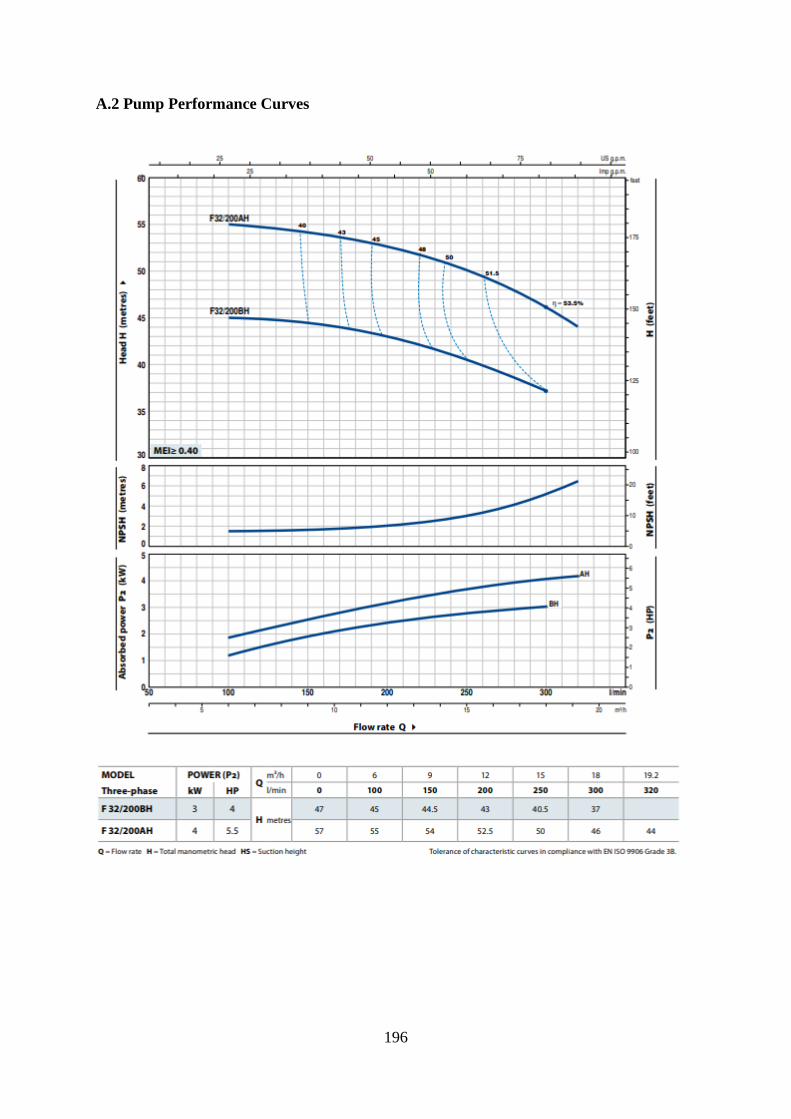
196

A.2 Pump Performance Curves

FINAL THESIS - Alabied.pdf

Documents

Transcript of FINAL THESIS - Alabied.pdf