
Revised Final Thesis Report - UQ eSpace
114
Revised Final Thesis Report “Evaluation of a blast damage model based on stress attenuation criteria” The University of Queensland Faculty of Engineering, Architecture and Information Technology School of Mechanical and Mining Engineering MINE4123 – Mining Research Project II Course Coordinator: Dr Chris Leonardi Project Supervisor: Dr Italo Onederra Prepared by: Jake Lewis Monday, 7 th of November 2016
-
Upload
khangminh22 -
Category
Documents
-
view
1 -
download
0
Transcript of Revised Final Thesis Report - UQ eSpace
Revised Final Thesis Report
“Evaluation of a blast damage model based on stress attenuation criteria”
The University of Queensland Faculty of Engineering, Architecture and Information Technology
School of Mechanical and Mining Engineering
MINE4123 – Mining Research Project II Course Coordinator: Dr Chris Leonardi Project Supervisor: Dr Italo Onederra
Prepared by:
Jake Lewis
Monday, 7th of November 2016

STATEMENT OF ORIGINALITY
To the best of my knowledge, I affirm that the content of the attached document is the original
work of the creator of this report. Any relevant utilised material that has been published
previously has been appropriately and accurately referenced.
_____________________
Jake Lewis
Page i
ABSTRACT
Empirical models still maintain a large presence in blast design practices despite developments
in progressively complex modelling techniques to describe blast damage. This can be attributed
to the heterogeneity of rock masses and the related difficulties associated with obtaining the
accuracy level required of higher order models within the practical constraints of time and cost.
Although empirical blast damage models may have the tendency to misrepresent the
importance of critical defining parameters leading to less than accurate outcomes. Where
inappropriately sensitive to certain properties, empirical blast damage models can result in less
than optimal blast design parameters. This research project aimed to evaluate a new empirical
blast damage model developed by Onederra (2016) that has been designated as the iDamage
model. This model utilises a stress attenuation function and a tensile strength limiting criteria
to yield an estimate for radius of fracturing induced by a single charge.
The evaluation consisted of making comparisons to existing empirical models, in terms of
damage output as well as in the application of these models to determine estimates for
fundamental blast design properties. It was determined that the iDamage model appropriated
the changes in the rock mass and explosive characteristics in a more stable capacity, yielding
a more central estimate of fracture radii relative to other empirical models. The scenario for a
120mm charge radius in fully confined conditions, for an emulsion product (VOD = 5500m/s)
in hard rock is a good representation of this observation. The iDamage model projected a
fracture radius of 2.9m while other empirical model estimates gave a range of values between
1.9m and 4.0mThis was further supported by comparison to the damage limits determined from
a range of practical case studies. Where the average deviation from the practical scenario was
0.35m for the iDamage models but was as high as 1.75m for other empirical methods. This
tendency was also observed when using the damage limits of the iDamage model to determine
estimates for blast design parameters. An initial sensitivity analysis generally demonstrated
high sensitivity of the iDamage model to parameters that described both the rock mass and
explosive (such as σT and VOD). However, for lower yield explosives, explosive characteristics
were relatively more sensitive. Based on the often balanced sensitivity to input parameters and
relative centrality of damage estimates the iDamage model was proposed to be an effective
tool to supplement the initial processes involved in blast design..
Page ii
CONTENTS
STATEMENT OF ORIGINALITY .................................................................................................................... 2
ABSTRACT .......................................................................................................................................................... I
CONTENTS ......................................................................................................................................................... II
LIST OF FIGURES ............................................................................................................................................ IV
LIST OF TABLES .............................................................................................................................................. VI
1. INTRODUCTION ....................................................................................................................................... 1
1.1 PROJECT OVERVIEW ............................................................................................................................... 1
1.2 AIMS AND OBJECTIVES ............................................................................................................................ 1
1.3 SCOPE ....................................................................................................................................................... 2
1.4 SIGNIFICANCE AND RELEVANCE TO INDUSTRY ...................................................................................... 3
2. OVERVIEW OF THE iDAMAGE BLAST DAMAGE MODEL ............................................................ 5
3. LITERATURE REVIEW ........................................................................................................................... 9
3.1 INTRODUCTION ........................................................................................................................................ 9
3.2 ROCK STRENGTH AND AFFILIATED PROPERTIES................................................................................... 9
3.2.1 Static Properties and Empirical Tensile Strength Relationships .................................................... 9
3.2.2 Dynamic Properties and Empirical Relationships ........................................................................ 11
3.3 ROCK BREAKAGE MECHANISM BY BLASTING ..................................................................................... 14
3.3.1 Explosive Detonation .................................................................................................................... 14
3.3.2 Transfer of Explosive Energy to Rock Mass ................................................................................. 16
3.3.2.1 Breakage due to stress waves .............................................................................................................. 17
3.3.2.2 Breakage due to gas expansion ........................................................................................................... 18
3.3.2.3 Breakage mechanism dominance ........................................................................................................ 18
3.3.3 The impact of geotechnical features on rock breakage................................................................. 19
3.4 EXISTING EMPIRICAL BLAST DAMAGE MODELS ................................................................................. 21
3.4.1 Holmberg-Persson Method ........................................................................................................... 23
3.4.2 Lu-Hustrulid Method .................................................................................................................... 24
3.4.3 Russian Method ............................................................................................................................ 25
3.4.4 Senuk Method ................................................................................................................................ 26
3.5 CONCLUSION .......................................................................................................................................... 26
4. PROJECT METHODLOGY ................................................................................................................... 28
4.1 EVALUATION METHODOLOGY .............................................................................................................. 28
4.1.1 Rock mass data and explosive properties determination .............................................................. 28
4.1.2 Comparison of empirical blast damage models ............................................................................ 30
4.1.3 Sensitivity analysis of the iDamage model .................................................................................... 31
4.1.4 Case study evaluation with iDamage model ................................................................................. 33
Page iii
4.1.5 Application of iDamage model to determine blast design parameters ......................................... 34
4.2 RISK MANAGEMENT .............................................................................................................................. 34
4.2.1 Contingency Plans ........................................................................................................................ 38
4.3 EVALUATION OF PROJECT MANAGEMENT ........................................................................................... 39
5. COMPARISON OF EMPIRICAL MODELS AND SENSITIVITY OF THE iDAMAGE MODEL . 40
5.1 INTRODUCTION ...................................................................................................................................... 40
5.2 COMPARISON OF EMPIRICAL MODEL PREDICTIONS ........................................................................... 40
5.2.1 Graphical Analysis of Empirical Comparison .............................................................................. 42
5.3 SENSITIVITY ANALYSIS OF THE iDAMAGE MODEL ............................................................................... 52
5.4 CONCLUSION .......................................................................................................................................... 56
6. CASE STUDY EVALUATION................................................................................................................ 58
6.1 INTRODUCTION ...................................................................................................................................... 58
6.2 CASE STUDY SYNOPSES ......................................................................................................................... 58
6.3 ANALYSIS OF CASE STUDIES ................................................................................................................. 59
6.4 CONCLUSION .......................................................................................................................................... 61
7. EMPIRICAL MODELS TO DETERMINE BLAST DESIGN PARAMETERS (OPEN PIT) .......... 62
7.1 BURDEN ESTIMATES FOR GENERAL SCENARIOS.................................................................................. 63
7.2 BURDEN AND SPACING ESTIMATES FOR CASE STUDY DATA ............................................................... 66
8. CONCLUSIONS AND RECOMMENDATIONS .................................................................................. 70
8.1 CONCLUSIONS ........................................................................................................................................ 70
8.2 RECOMMENDATIONS ............................................................................................................................. 73
9. REFERENCES .......................................................................................................................................... 75
APPENDIX A. TYPICAL ROCK MASS PROPERTIES ............................................................... 81
APPENDIX B. PPV DAMAGE CRITERION ................................................................................. 83
APPENDIX C. PROJECT SCHEDULE .......................................................................................... 85
APPENDIX D. EMPIRICAL COMPARISON SUPPLEMENTARY INFORMATION ............. 86
APPENDIX E. SENSITIVITY ANALYSIS SUPPLEMENTARY INFORMATION .................. 91
APPENDIX F. BURDEN ESTIMATION SUPPLEMENTARY INFORMATION. .................. 102
Page iv
LIST OF FIGURES
Figure 1. iDamage model estimation methodology (Onederra, 2016) .................................................................... 5 Figure 2. Charge length assumption ....................................................................................................................... 8 Figure 3. Relative velocities of p-wave to s-wave propagation (modified from Erickson, 2014) ........................ 12 Figure 4. Impact of homogeneity on tensile strength (Cho, Kaneko and Ogata, 2003) ........................................ 13 Figure 5. CJ Explosive detonation (modified from Erickson, 2014) .................................................................... 15 Figure 6. Phases of blast damage loading (Brady and Brown, 2004) ................................................................... 16 Figure 7. Rock breakage due to stress limits (Erickson, 2014) ............................................................................. 17 Figure 8. Breakage processes for (left) stress wave and (right) gas expansion (Modified from Sharma, 2012) .. 19 Figure 9. Holmberg-Persson model geometry (Sun, 2013) .................................................................................. 24 Figure 12. Stress attenuation constant determination (Esen and Onederra, 2004) ................................................ 30 Figure 10. Sensitivity and uncertainty representation (Dijkman, Stedinger, and Villars, 2005)........................... 31 Figure 11. Deterministic input layout (Dijkman, Stedinger, and Villars, 2005) ................................................... 32 Figure 13. Comparison of Lu-Hustrulid to iDamage model - Emulsion A........................................................... 44 Figure 14. Comparison of Lu-Hustrulid to iDamage model - Emulsion B ........................................................... 44 Figure 15. Comparison of Lu-Hustrulid to iDamage model - ANFO ................................................................... 45 Figure 16. Comparison of Holmberg-Persson to iDamage model - Emulsion A.................................................. 46 Figure 17. Comparison of Holmberg-Persson to iDamage model - Emulsion B .................................................. 46 Figure 18. Comparison of Holmberg-Persson to iDamage model - ANFO .......................................................... 47 Figure 19. Comparison of Russian model to iDamage model - Emulsion A ........................................................ 48 Figure 20. Comparison of Russian model to iDamage model - Emulsion B ........................................................ 48 Figure 21. Comparison of Russian model to iDamage model - ANFO ................................................................ 49 Figure 22. Comparison of Senuk model to iDamage model - Emulsion A .......................................................... 50 Figure 23. . Comparison of Senuk model to iDamage model - Emulsion B ......................................................... 50 Figure 24. . Comparison of Senuk model to iDamage model - ANFO ................................................................. 51 Figure 25. Tornado plot for hard rock - emulsion A ............................................................................................. 53 Figure 26. Tornado plot for medium rock - emulsion A ....................................................................................... 53 Figure 27 . Tornado plot for soft rock - emulsion A ............................................................................................. 54 Figure 28. Spider plot for hard rock - emulsion A ................................................................................................ 54 Figure 29. Spider plot for medium rock - emulsion A .......................................................................................... 55 Figure 30. Spider plot for soft rock - emulsion A ................................................................................................. 55 Figure 31. Comparison of empirical models to practical data .............................................................................. 60 Figure 32. Burden estimates for emulsion A - hard rock ...................................................................................... 64 Figure 33. Burden estimates for emulsion A - medium rock ................................................................................ 65 Figure 34. Burden estimates for emulsion A - soft rock ....................................................................................... 65 Figure 35. Burden estimation comparison for case studies .................................................................................. 68 Figure 36. Spacing estimation comparison for case studies ................................................................................. 68 Figure 37. Shear modulus ranges (Schon, 2011) .................................................................................................. 81 Figure 38. Poisson's ratio ranges (Schon, 2011) ................................................................................................... 81 Figure 39. UCS ranges (Schon, 2011) .................................................................................................................. 82 Figure 40. Full research project schedule ............................................................................................................. 85 Figure 41. Tornado plot for hard rock - emulsion B ............................................................................................. 97 Figure 42. Tornado plot for medium rock - emulsion B ....................................................................................... 97 Figure 43. Tornado plot for soft rock - emulsion B .............................................................................................. 97 Figure 44. Tornado plot for hard rock – ANFO.................................................................................................... 98 Figure 45. Tornado plot for medium rock – ANFO .............................................................................................. 98 Figure 46. Tornado plot for soft rock - ANFO ..................................................................................................... 98 Figure 47. Spider plot for hard rock - emulsion B ................................................................................................ 99 Figure 48. Spider plot for medium rock - emulsion B .......................................................................................... 99 Figure 49. Spider plot for soft rock - emulsion B ............................................................................................... 100 Figure 50. Spider plot for hard rock - ANFO ..................................................................................................... 100 Figure 51. Spider plot for medium rock – ANFO ............................................................................................... 101 Figure 52. Spider plot for soft rock - ANFO ...................................................................................................... 101 Figure 53. Burden estimates for emulsion B - hard rock .................................................................................... 104 Figure 54. Burden estimates for emulsion B - medium rock .............................................................................. 104 Figure 55. Burden estimates for emulsion B - soft rock ..................................................................................... 105 Figure 56. Burden estimates for ANFO - hard rock ........................................................................................... 105

Page v
Figure 57. Burden estimates for ANFO - medium rock ..................................................................................... 106 Figure 58. Burden estimates for ANFO - soft rock ............................................................................................ 106
Page vi
LIST OF TABLES
Table 1. Input parameters required for iDamage model ......................................................................................... 6 Table 2. Existing empirical blast damage models summarised ........................................................................... 22 Table 3. Rock mass compressive strength categorisation .................................................................................... 29 Table 4. Probability Factor (modified BHP, 2009) .............................................................................................. 35 Table 5. Severity Factor (modified BHP, 2009) .................................................................................................. 35 Table 6. Risk categorisation matrix (modified BHP, 2009) ................................................................................ 36 Table 7. Risk management plan used throughout research project ...................................................................... 37 Table 8. Contingencies and reaction plans .......................................................................................................... 38 Table 9. Fundamental Rock Mass Properties ...................................................................................................... 41 Table 10. Explosive configuration parameters .................................................................................................... 41 Table 11. Summary of Comparison Results ........................................................................................................ 43 Table 12. Sensitivity analysis priority order ........................................................................................................ 56 Table 13. Case study model input parameters (Esen and Onederra, 2004) ......................................................... 59 Table 14. Empirical damage estimates for case studies ....................................................................................... 59 Table 15. Burden estimation functions ................................................................................................................ 62 Table 16. Burden data estimates for general comparison - emulsion A .............................................................. 63 Table 17. Burden estimation data for case studies ............................................................................................... 67 Table 18. Spacing estimation data for case studies .............................................................................................. 67 Table 19. Typical comparison between empirical blast damage models at 120mm ............................................ 70 Table 20. Dynamic and static compressive strengths (Sun, 2013) ....................................................................... 81 Table 21. Common compressive, tensile and shear stresses (Attewell and Farmer, 1976) .................................. 82 Table 22. Bauer and Calder PPV limits (Narendrula and Singh, 2004)................................................................ 83 Table 23. Holmberg PPV limits (Narendrula and Singh, 2004) ........................................................................... 83 Table 24. Adhikari PPV limits (Narendrula and Singh, 2004) ............................................................................. 83 Table 25. Jimeno PPV limits (Narendrula and Singh, 2004) ................................................................................ 83 Table 26. Tunstall's open pit PPV limits (Narendrula and Singh, 2004) .............................................................. 83 Table 27. Singh's underground PPV limits (Narendrula and Singh, 2004) ......................................................... 84 Table 28. Critical PPV limits (Narendrula and Singh, 2004) ............................................................................... 84 Table 29. Rock mass data source information ..................................................................................................... 86 Table 30. Explosive properties source information ............................................................................................. 86 Table 31. Rock mass/explosive properties reference guide ................................................................................. 87 Table 32. Empirical blast damage estimates using Emulsion A .......................................................................... 88 Table 33. Empirical blast damage estimates using emulsion B ........................................................................... 89 Table 34. Empirical blast damage estimates using ANFO ................................................................................... 90 Table 35. Sensitivity analysis rock mass data - emulsion A ................................................................................ 91 Table 36. Sensitivity analysis explosive properties data - emulsion A ................................................................ 92 Table 37. Sensitivity analysis rock mass data - emulsion B ................................................................................ 93 Table 38. Sensitivity analysis explosive properties data - emulsion B ................................................................ 94 Table 39. Sensitivity analysis rock mass data – ANFO ....................................................................................... 95 Table 40. Sensitivity analysis explosive properties data – ANFO ....................................................................... 96 Table 41. Burden estimation data for general comparison - emulsion B ........................................................... 102 Table 42. Burden estimation data for general comparison – ANFO .................................................................. 103
Page 1
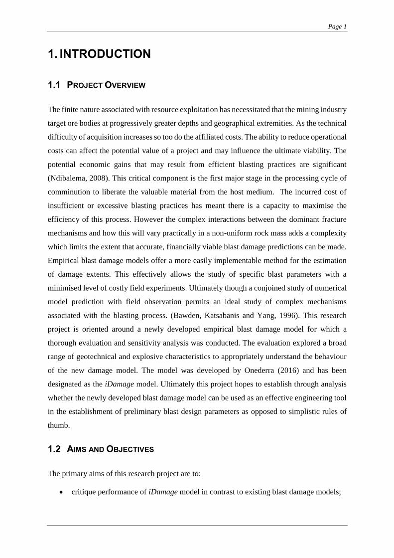
1. INTRODUCTION
1.1 PROJECT OVERVIEW
The finite nature associated with resource exploitation has necessitated that the mining industry
target ore bodies at progressively greater depths and geographical extremities. As the technical
difficulty of acquisition increases so too do the affiliated costs. The ability to reduce operational
costs can affect the potential value of a project and may influence the ultimate viability. The
potential economic gains that may result from efficient blasting practices are significant
(Ndibalema, 2008). This critical component is the first major stage in the processing cycle of
comminution to liberate the valuable material from the host medium. The incurred cost of
insufficient or excessive blasting practices has meant there is a capacity to maximise the
efficiency of this process. However the complex interactions between the dominant fracture
mechanisms and how this will vary practically in a non-uniform rock mass adds a complexity
which limits the extent that accurate, financially viable blast damage predictions can be made.
Empirical blast damage models offer a more easily implementable method for the estimation
of damage extents. This effectively allows the study of specific blast parameters with a
minimised level of costly field experiments. Ultimately though a conjoined study of numerical
model prediction with field observation permits an ideal study of complex mechanisms
associated with the blasting process. (Bawden, Katsabanis and Yang, 1996). This research
project is oriented around a newly developed empirical blast damage model for which a
thorough evaluation and sensitivity analysis was conducted. The evaluation explored a broad
range of geotechnical and explosive characteristics to appropriately understand the behaviour
of the new damage model. The model was developed by Onederra (2016) and has been
designated as the iDamage model. Ultimately this project hopes to establish through analysis
whether the newly developed blast damage model can be used as an effective engineering tool
in the establishment of preliminary blast design parameters as opposed to simplistic rules of
thumb.
1.2 AIMS AND OBJECTIVES
The primary aims of this research project are to:
critique performance of iDamage model in contrast to existing blast damage models;
Page 2
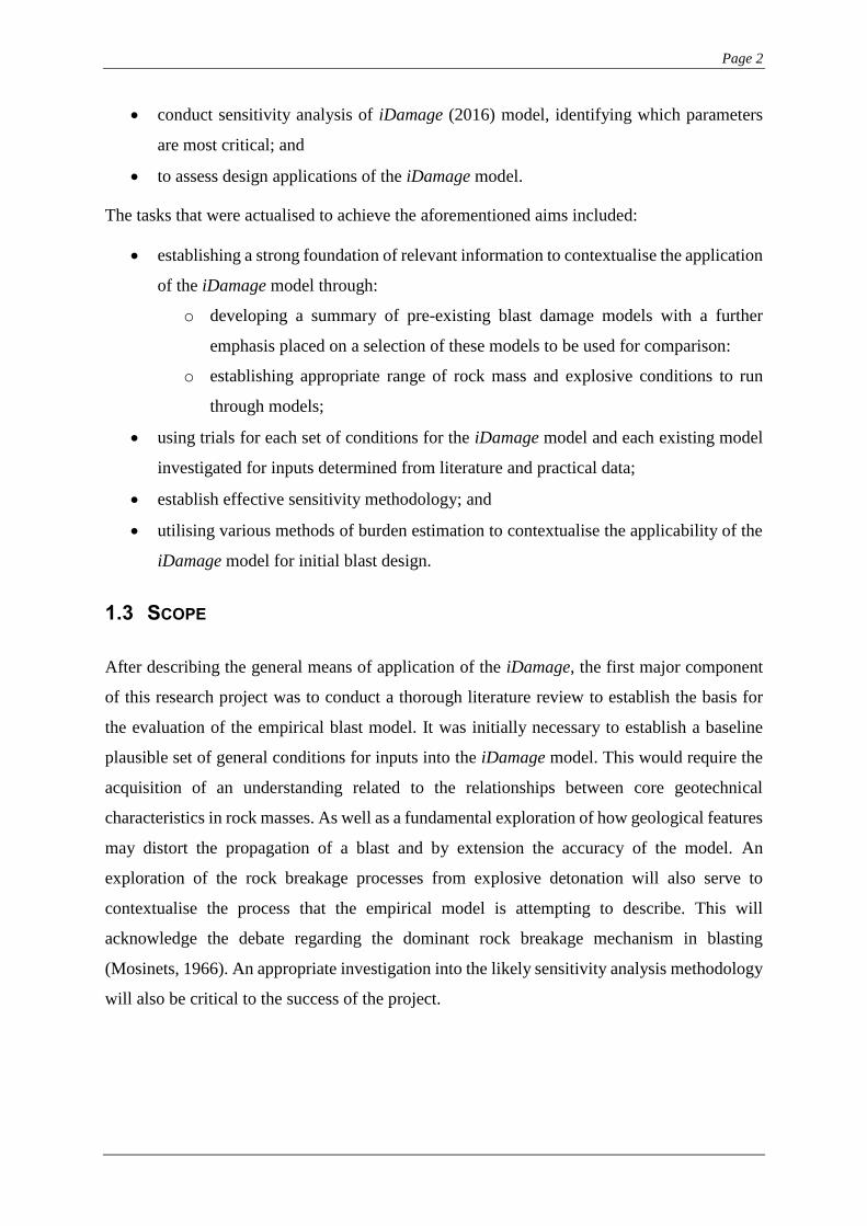
conduct sensitivity analysis of iDamage (2016) model, identifying which parameters
are most critical; and
to assess design applications of the iDamage model.
The tasks that were actualised to achieve the aforementioned aims included:
establishing a strong foundation of relevant information to contextualise the application
of the iDamage model through:
o developing a summary of pre-existing blast damage models with a further
emphasis placed on a selection of these models to be used for comparison:
o establishing appropriate range of rock mass and explosive conditions to run
through models;
using trials for each set of conditions for the iDamage model and each existing model
investigated for inputs determined from literature and practical data;
establish effective sensitivity methodology; and
utilising various methods of burden estimation to contextualise the applicability of the
iDamage model for initial blast design.
1.3 SCOPE
After describing the general means of application of the iDamage, the first major component
of this research project was to conduct a thorough literature review to establish the basis for
the evaluation of the empirical blast model. It was initially necessary to establish a baseline
plausible set of general conditions for inputs into the iDamage model. This would require the
acquisition of an understanding related to the relationships between core geotechnical
characteristics in rock masses. As well as a fundamental exploration of how geological features
may distort the propagation of a blast and by extension the accuracy of the model. An
exploration of the rock breakage processes from explosive detonation will also serve to
contextualise the process that the empirical model is attempting to describe. This will
acknowledge the debate regarding the dominant rock breakage mechanism in blasting
(Mosinets, 1966). An appropriate investigation into the likely sensitivity analysis methodology
will also be critical to the success of the project.
Page 3
The project methodology would also touch on the overarching strategy of project scheduling
and risk management that guided this research project. The various limitations of this scope
pertain to:
the range of parameter inputs considered for each empirical analysis;
the lack of access to numerical modelling facilities to support any conclusions;
the exclusion of high order sensitivity methodologies or the use of artificial neural
networks; and
no scale experimentation was undertaken with the specific purpose of evaluating this
model in mind.
Hence, any conclusions technically can only be said to be representative of within the
constraints of this scope.
1.4 SIGNIFICANCE AND RELEVANCE TO INDUSTRY
The nature of the iDamage model proposes a significant potential benefit to industry as it could
present a more accurate preliminary blast estimate to contribute to blast design and
optimisation. Once this study confirms the parameters on which this model is most reliant, a
case for the ideal conditions for application of this model may be made. As blasting serves as
one of the major primary contributors to the mining cost (Ndibalema, 2008) it is clear that an
empirical blast damage model, which can define a more accurate envelope, may potentially
increase the overall efficiency of the blast design process. By reducing unwanted blast damage
outcomes the potential gains that can be made includes: improved safety, reduction in
secondary blasting, smooth walls facilitating better ventilation and improved roof/wall
stability. (Sun,2013) In recent years, great strides have been made to developments in complex
numerical models, hybrid stress blasting models and mechanistic blasting models (Zhang,
2016). The application of these have the extended advantages of providing a highly detailed
representation of the interactions between the host rock mass, the stress waves resulting from
detonation and potentially the implications of gas expansion. However the quality of output
from said models is contingent on the level of accuracy associated with the required input
parameters (An and Ma, 2008). Otherwise, the specific demonstration of the analysed condition
will be an inappropriate representation of the reality it attempts to convey. The potential
regional variations of rock masses over an area mean that accurate quantification of geological
Page 4
intrusions, anisotropy and any discontinuities can be costly and time intensive to quantify. With
this in mind, the economic constraints of an efficient blasting operation cannot sustain the level
of survey required to constantly use numerical modelling. As a result semi-mechanistic and
empirical models continue to dominate the blast engineering design process. Where experience
based design criteria, to be efficient, have demonstrated dependable results in mining
applications to date (Esen and Onederra, 2014). In the instance of the new empirical blast
damage models demonstration of a more accurate value for the radius of fracture, the
advantages would translate to blast design efficiency in terms of burden and spacing
configurations. An advantage that the iDamage model yields over the dominant Holmberg-
Persson based methods is that it does not rely on site specific attenuation constants. These
constants vary regionally, having a large variation on the output of the model and must be
determined by PPV data from site. The absence of this dependency on constants simplifies the
applicability of the iDamage model. Concurrently, were this project to verify that iDamage
model can provide comparable damage envelopes to existing empirical estimation processes
there is a true capability to benefit the blast design engineering process.
Page 5
2. OVERVIEW OF THE iDAMAGE BLAST DAMAGE
MODEL
The iDamage model was developed by Onederra in 2016 and is comprised of two elements.
Those elements are:
a pressure attenuation function and;
a tensile strength limiting criteria.
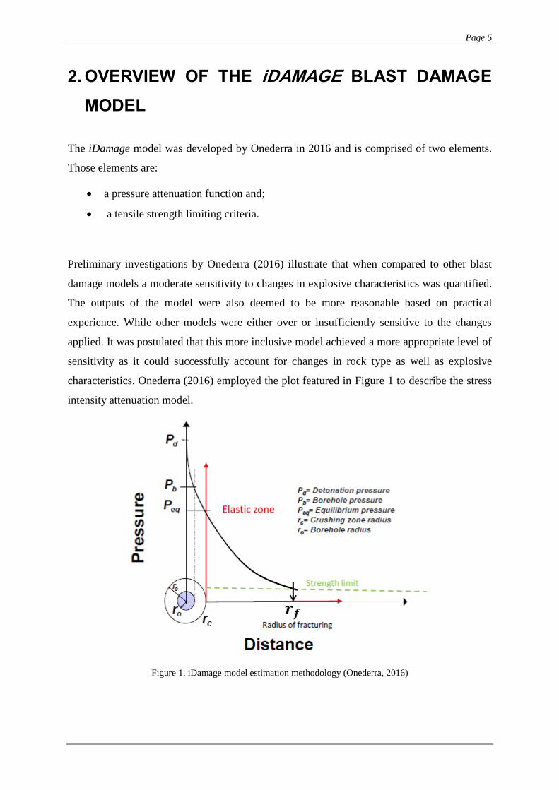
Preliminary investigations by Onederra (2016) illustrate that when compared to other blast
damage models a moderate sensitivity to changes in explosive characteristics was quantified.
The outputs of the model were also deemed to be more reasonable based on practical
experience. While other models were either over or insufficiently sensitive to the changes
applied. It was postulated that this more inclusive model achieved a more appropriate level of
sensitivity as it could successfully account for changes in rock type as well as explosive
characteristics. Onederra (2016) employed the plot featured in Figure 1 to describe the stress
intensity attenuation model.
Figure 1. iDamage model estimation methodology (Onederra, 2016)
Page 6
Fundamentally, the pressure of equilibrium is used to set the bounds of the elastic zone by
acting as the starting point for the attenuation of peak stress. The estimation of this pressure
will be contingent on both the detonation and borehole pressures. The radius of fracture may
then be identified at the intersection of the tensile strength limiting criteria in the elastic zone.
(Onederra, 2016) The inputs of the function are arranged in Table 1.
Table 1.
Input parameters required for iDamage model
Required Inputs
Explosive Based Geotechnically Based
Charge Diameter UCS
VOD UTS
Explosive Density Rock material density Vp-wave
Poisson’s Ratio
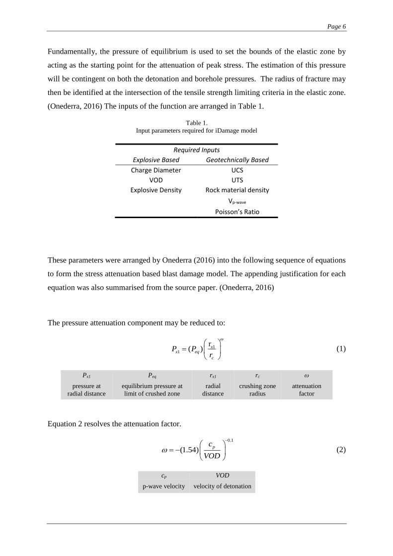
These parameters were arranged by Onederra (2016) into the following sequence of equations
to form the stress attenuation based blast damage model. The appending justification for each
equation was also summarised from the source paper. (Onederra, 2016)
The pressure attenuation component may be reduced to:
11
r( ) x
x eq
c
P Pr
(1)
Px1 Peq rx1 rc ω
pressure at
radial distance
equilibrium pressure at
limit of crushed zone
radial
distance
crushing zone
radius
attenuation
factor
Equation 2 resolves the attenuation factor.
0.1
(1.54)pc
VOD
(2)
cp VOD
p-wave velocity velocity of detonation
Page 7
Equations 3 and 4 allow the estimation of the equilibrium pressure at the limit of the crushed
zone. The pressure decay factor considers the rock mass and the explosive.
r
r
ceq b
o
P P
, where
0.33
(1.54)pc
VOD
(3, 4)
Pb ro ϕ
borehole pressure charge radius pressure decay factor
To arrive at the borehole pressure the detonation pressure must also be defined.
2
CJb
PP , where
2( )( )
4
oCJ
VODP
(5, 6)
PCJ ρo
detonation pressure unreacted explosive density
The method of estimating the crushing radius employed in this pressure attenuation function is
largely defined by the crushing zone index (CZI).
0.219(0.812)( )cr CZI (7)
The index itself, which depicts the crushing potential of the respective material, is established
in Equation 8.
3
2( )( )
b
c
PCZI
K (8)
K σc
rock stiffness UCS
Caution must be applied for instances of low CZI as this may lead to a ratio between the charge
radius and the crush radius that is greater than 1. This is an extraneous solution and physically
impossible. Situations of small CZI that could generate such a scenario may feature high
strength rock and decoupled charges. (Onederra, 2016)
1
dEK
(9)
Ed υ
dynamic Young’s modulus Poisons ratio
Page 8
As well as the rock stiffness, the tensile strength limit is a property of the rock mass that is
necessary to utilise this blast damage model. While there are relationships to estimate the
tensile strength from other parameters (Cai, 2010) practical tests may provide a higher level of
accuracy.
It is critical to note that the charge length has been neglected from the explosive input
parameters. The empirical model does not consider three dimensions and hence cannot take
iniation or boundary conditions into account. Concurrently the charge lengths analysed will
have already achieved the maximum VOD actualised by the explosive. This relationship is
effectively summarised in Figure 2.
Figure 2. Charge length assumption
This peak VOD achievable by the charge length is stable for the majority of charge lengths
past a certain threshold. Hence, this assumption will only be critical for very shallow charge
lengths (Onederra, 2016). This condition should be considered when applying the iDamage
model to establish initial blast design estimates.
Relationships to determine tensile strength from compressive strength are effective as a
baseline. Once the tensile strength is determined and the pressure attenuation function
completed the radius of fracturing can be identified.
Vel
oci
ty o
f D
eto
nat
ion
Charge Length
Charge Length Assumption Justification
VOD-Charge length Maximum VOD
Page 9
3. LITERATURE REVIEW
3.1 INTRODUCTION
In order to develop the understanding of the stress attenuation model it will be necessary to
investigate the core principles influencing the predictive outcome as well as the strategies to
be employed by the sensitivity analysis. The specific research objectives of which this literature
review is comprised are to:
understand the relevant properties that determine the behaviour of the intact rock mass;
explore the mechanisms of how rock fracture occurs as a result of blast hole detonation;
determine how geotechnical/geological features can influence the propagation of blast
damage;
identify and assess blast damage models that have already been devised; and to
investigate sensitivity analysis strategies that could be applied to the geotechnical
properties of the blast damage model.
These objectives have been structured to provide relevant background information to
supplement conclusions and to facilitate the evaluation of the iDamage model
3.2 ROCK STRENGTH AND AFFILIATED PROPERTIES
For the purpose of this analysis, the representative rock mass properties will be assumed to be
for an isotropic case. This will provide a more continuous means of comparison between
findings as empirical models often will not have a tangible means of appropriating the regional
variation of a non-ideal rock mass which in turn will go on to effect blast performance. To
investigate the relationships between the parameters describing the predicted radius of
fracturing it is critical to comprehend the base geotechnical properties that govern rock
strength. Any relationships established between properties will supplement any conclusions to
come from the sensitivity analysis as a case for the dependency between the parameters can be
identified.
3.2.1 Static Properties and Empirical Tensile Strength Relationships
The major static properties of rock strength are chiefly confined to compressive strength,
tensile strength, shear strength, density, Young’s modulus and poison’s ratio. (Duan, Kwok
Page 10
and Tham, 2013) They are quantified as being static properties when the loading condition is
not variable over any significant period.
Previous studies have defined relationships between some static properties of rock which may
serve as effective starting points of estimation. This illustrates a degree of dependency between
these properties. However these trends typically change slightly based on the rock type and
concurrently there is no perfect correlation that can be relied on. The tensile strength limiting
criteria is a core component of the iDamage model. Diedrichs and Perras (2013) conducted a
review into estimation of tensile strength from other properties. Due to the instability of tensile
fracturing under tensile loading, there are difficulties with direct tensile testing. Some of the
correlation formulae evaluated in this study include:
501.5( )t IS , where 50(16 24)( )c IS (10, 11)
Alternatively, the simplification of setting the minimum principle stress to 0 achieves Equation
(12) which is based on the pressure associated with crack initiation. Crack initiation represents
the first onset of new distributed grain scale cracks within the specimen during testing.
(Diedrichs and Perras, 2013)
t
CI
(12)
Note that β is a constant that ranges from 8-12. For strong brittle rocks it is often assumed that
β is 8. This value can be more accurately determined for brittle rocks by:
cG
ci
(13)
Where βG is a constant equal to 8, taken from Griffith’s method. Other estimation methods
include
'
(0.5)t
c
E
L
, where
2'
1
EE
and
2
(14)
Lc γ
crack length Specific surface energy
And
(12)t c (15)
Page 11
Critically though, Griffith’s theory and Murrell’s criterion in equations 14 and 15 respectively
are quite dated and do not effectively account for changes in rock type. (Cai, 2010)
The crack initiation stress in tension is close to its peak strength. The crack initiation strength
in compression is much lower than the peak strength (Cai, 2010). It was posited that estimation
by UCS yielded the most erroneous correlations. While using the crack initiation limits and
damage thresholds to identify tensile strength yielded a closer value. (Diedrichs and Perras,
2013). The data used to reach these conclusions admittedly had a significant range of scatter
However, the advantage of the UCS is the error associated with peak UCS is only a few percent
while σci can be as high as 15% (Cai, 2010). The rock type cannot be used to directly define
strength and data inferred from databases is only appropriate at an initial design stage. Cai
(2010) asserts that the approach using equations (13) and (14) is proximal to derivations of
tensile strength from the Brazilian tests based on tests with most errors being less than 15%.
Based on this finding it is believed that this represents the best empirical means of determining
tensile strength.
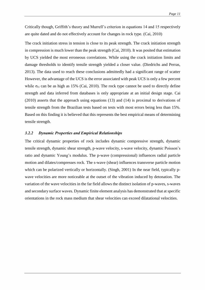
3.2.2 Dynamic Properties and Empirical Relationships
The critical dynamic properties of rock includes dynamic compressive strength, dynamic
tensile strength, dynamic shear strength, p-wave velocity, s-wave velocity, dynamic Poisson’s
ratio and dynamic Young’s modulus. The p-wave (compressional) influences radial particle
motion and dilates/compresses rock. The s-wave (shear) influences transverse particle motion
which can be polarized vertically or horizontally. (Singh, 2001) In the near field, typically p-
wave velocities are more noticeable at the outset of the vibration induced by detonation. The
variation of the wave velocities in the far field allows the distinct isolation of p-waves, s-waves
and secondary surface waves. Dynamic finite element analysis has demonstrated that at specific
orientations in the rock mass medium that shear velocities can exceed dilatational velocities.
Page 12
Figure 3. Relative velocities of p-wave to s-wave propagation (modified from Erickson, 2014)
Despite p-wave velocity dominance in the near field, if an empirical model were neglect the s-
wave component entirely it must be acknowledged that a component of the ground movement
has not been accounted for. In some configurations, this omission may create a disparity
between the practical condition and that identified by the model (Erickson, 2014).
As the loading characteristic has changed, it is anticipated that there will be a variation in the
predicted response. Dhawan and Muralidhar (2015) define the following empirical
relationships to estimate dynamic Poisson’s ratio and dynamic Young’s modulus.
2 2
2 2
( 2 )
2( )
p s
d
p s
c c
c c
(16)
2 (1 )(1 2 )
(1 )
d dd p
d
E c
(17)
cs υd
s-wave velocity dynamic Poisson’s ratio
Empirical formulae have been derived to determine an estimate for static UCS from the p-wave
velocity. Multiple trends have been defined to accommodate various collections of rock types.
Sharma and Singh (2007) have assessed some of the relatively more widely accurate functions
Page 13
based on a wide selection of rock samples. The ideal function was identified as a linear
relationship.
(0.0642) 117.99c pc (18)
The frequency of points in these tests and the significant variation between rock types create a
high potential for outliers. While this trend is still one of the more accurate possible
relationships, its simplicity limits its overall applicability.
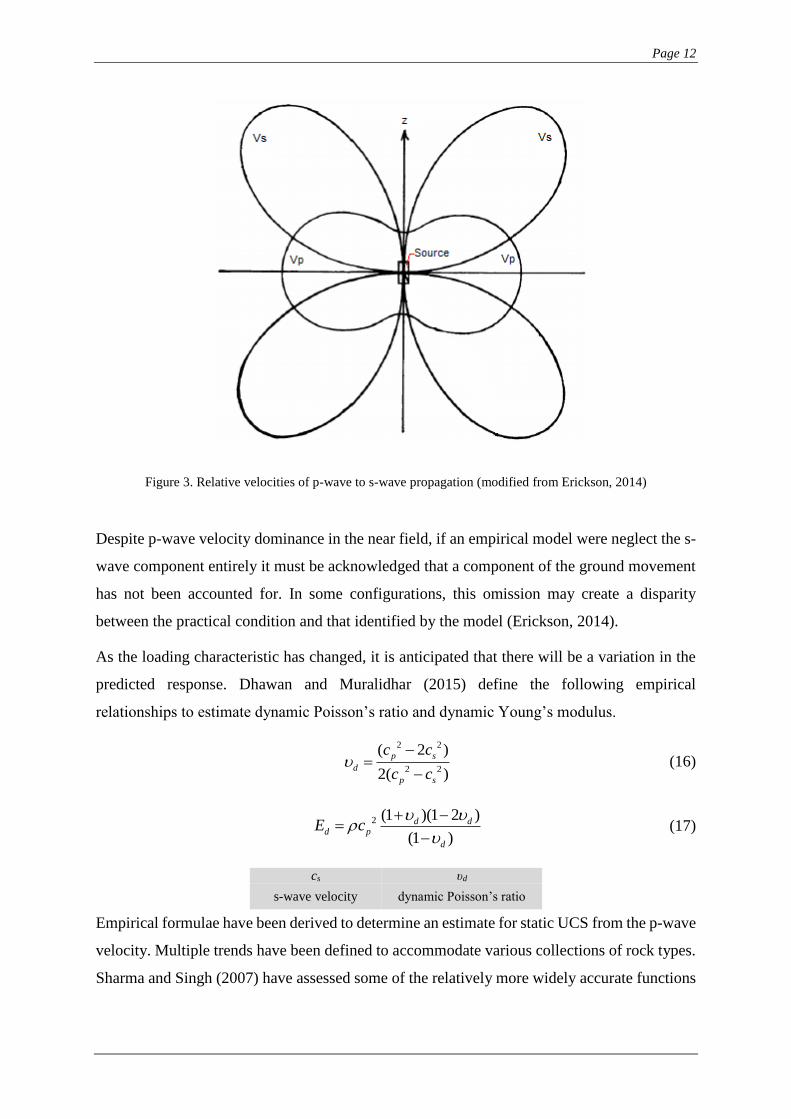
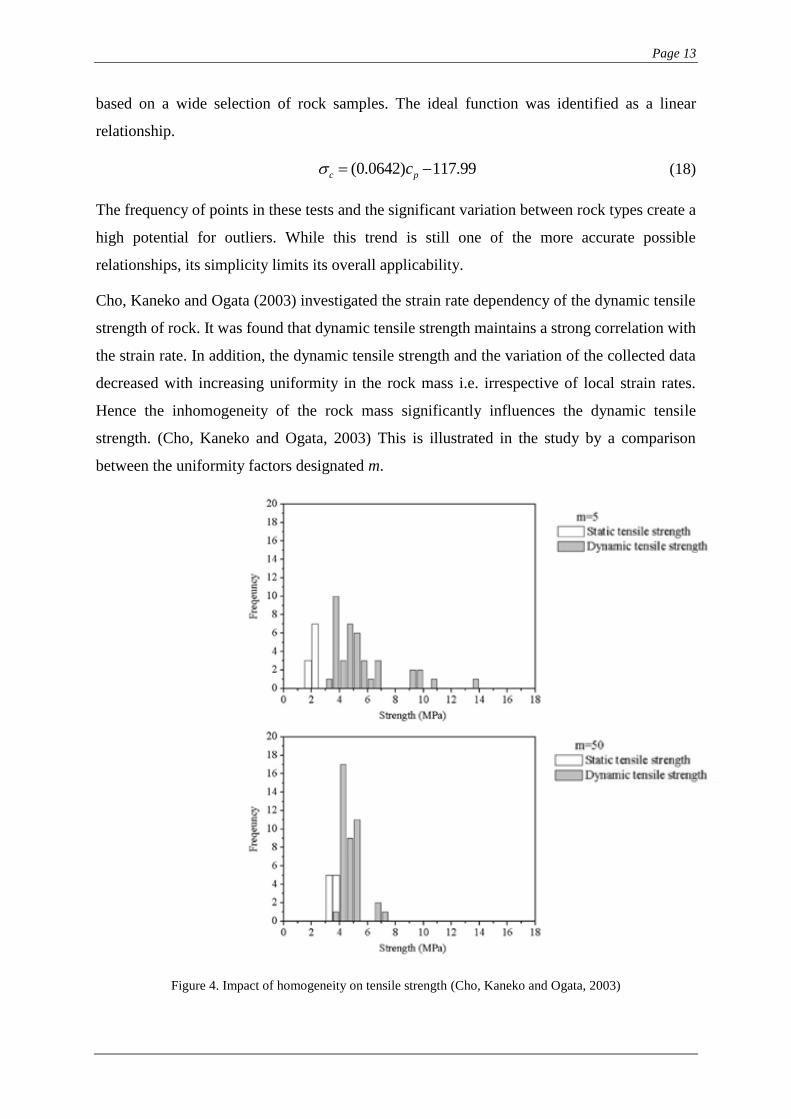
Cho, Kaneko and Ogata (2003) investigated the strain rate dependency of the dynamic tensile
strength of rock. It was found that dynamic tensile strength maintains a strong correlation with
the strain rate. In addition, the dynamic tensile strength and the variation of the collected data
decreased with increasing uniformity in the rock mass i.e. irrespective of local strain rates.
Hence the inhomogeneity of the rock mass significantly influences the dynamic tensile
strength. (Cho, Kaneko and Ogata, 2003) This is illustrated in the study by a comparison
between the uniformity factors designated m.
Figure 4. Impact of homogeneity on tensile strength (Cho, Kaneko and Ogata, 2003)
Page 14
Figure 4 demonstrates a sharp coalescence in the range of tensile strengths as homogeneity
increases. It is also observable that the magnitudes of dynamic tensile strengths are typically
higher than static tensile strengths as represented in these plots.
The dynamic compressive strength usually increases because of the strain rate effect. (Li, Lu
and Ma, 2010) From this point the dynamic compressive strength begins to increase
significantly at rock type dependent rate. The loading strain rates associated with blasting are
at least in advance of an order of 10 (Sun, 2013). A collection of the variations between static
and dynamic compressive strengths has been identified by a study undertaken by Sun (2013)
for various rock archetypes. This has been provided in Appendix A, Table 20. It should be
noted that Appendix A also features other typical rock mass properties for potential use in the
final sensitivity analysis. Irrespective of whether they are used in the final analysis, they
provide insight into the range of variability experienced by typical rock mass properties.
3.3 ROCK BREAKAGE MECHANISM BY BLASTING
To give context to the application of the iDamage model it is critical to understand what
interactions are taking place in the surrounding host rock once the explosive has been
detonated. While it is commonly accepted that the behaviour of explosive-rock interaction at a
base level is well known, research efforts remain to develop a more precise understanding of
this process (Zhang, 2016). This summary of this interaction will consist of a two part
explanation detailing:
the response of the explosive during detonation; and
how explosive energy is transferred to the rock mass to induce breakage.
It should be noted that this description attempts to provide a general overview of this process
to supplement the interpretation of results for estimated damage radii from the empirical
models to be analysed.
3.3.1 Explosive Detonation
Several approaches have been developed to accurately quantify the processes being executed
during explosive detonation. These vary from: one-dimensional analyses, direct numerical
solutions, detonation shock dynamics, equation of state for gas behaviour and streamline
approaches (Zhang, 2016). Given the objectives of this project, the one-dimensional methods
have been deemed sufficient for the purpose of this literature review, though it is important to
Page 15
acknowledge that this explanation will be predicated on some base assumptions. The most
prevalent one-dimensional theory to describe the behaviour of the explosive was defined as the
Chapman-Jouget (CJ) detonation theory. This process assumes that detonation and flow occur
in one dimension, it is ideal and only the chemical reaction itself is considered. The impact of
heat conduction, radiation, viscosity and diffusion in the explosive are not taken into account.
Also it is assumed that the chemical reaction will occur at a wave front and be completed
instantaneously (Zhang, 2016). At the point of detonation, a chemical reaction is instigated by
the detonator to release the chemical potential energy of the explosive. This massively
exothermic reaction converts the solid (or liquid) explosive into energy and gasses (Sharma,
2012). Figure 5 has been provided to assist in the demonstration of the CJ theory of detonation.
Figure 5. CJ Explosive detonation (modified from Erickson, 2014)
The explanation of this action as described by Sharma (2012) involves the conceptual CJ plane,
which is of negligible space, separating the unreacted explosive from the reacted heat and
gasses on the other as seen in Figure 5. This commences at Y as a rapid pressure, which may
generate the reaction by shock to the gas front at X. (Sharma, 2012). While the VOD along
this front ensures that the explosive in a typical blasting application will be consumed rapidly
(i.e. over a range of milliseconds). Explosives yielding higher velocities achieve higher
magnitude stress waves by quicker evolution of gaseous reaction products. This can be
influenced by several factors such as the confinement level in the borehole and charge diameter.
The influence of charge length however will only increase with VOD to a point before reaching
an equilibrium value, propagating across the explosive front. Once detonation commences a
convex, compressive shock wave acts along the borehole walls and through the explosive. This
Page 16
borehole pressure will drop considerably for decoupled conditions. While the CJ model is not
an absolute representation of reality due to the limitations imposed by the simplifying
assumptions, this essentially summarises the processes undertaken during explosive
detonation.
3.3.2 Transfer of Explosive Energy to Rock Mass
Once the energy from the explosive is translated to the rock mass, breakage is achieved through
a complex process of consequential and combinational interactions. These stages can be
broadly attributed to, stress wave propagation and gas expansion (Sharma, 2012).
A simplistic summary of the product of these processes loading mechanism is offered by Brady
and Brown (2004).
Figure 6. Phases of blast damage loading (Brady and Brown, 2004)
The phases of loading described by in Figure 6 from left to right are:
dynamic loading;
o occurs during explosive charge detonation;
o includes formation and propagation of body wave.
quasi-static loading; and
o under residual blasthole pressure applied by the reaction gases
loading release.
o occurs during period of rock displacement;
o transient stress field is relaxed
Once these phases of loading have concluded the blast hole will have expanded outwards into
the crush zone radius. (Brady and Brown, 2004).
Page 17
3.3.2.1 Breakage due to stress waves
The stress waves that result from the explosive detonation are attributed to the rising
temperature and frequency of gaseous products effecting a massive increase in pressure
transmitted into the confining rock mass. As the host rock initially has not had sufficient time
to balance that equilibrium by increasing volume appropriately. In the immediate vicinity of
the rock mass, fragmentation will occur where the stress waves exert a pressure greater than
that of the dynamic compressive strength of the rock mass. This stress will concurrently reach
a peak level and will follow this with a degree of exponential stress decay (Zhang, 2016). The
decay is attributed to the increased volume of the borehole, decreasing the pressure-based
interaction of the gaseous products with the surrounding rock mass. The rock mass can no
longer fail in compression outside the radius of damage established initially by the stress waves.
The initial stress pulse however results in a secondary tangential stress, which results in tensile
failure in the rock (Erickson, 2014). With increasing radial, distance from the borehole the
frequency of radial fractures induced by tensile failure decreases. A representation of the
failure modes actualised by stress waves for a fully confined borehole has been provided in
Figure 7.
Figure 7. Rock breakage due to stress limits (Erickson, 2014)
Within the crushed zone, breakage from dynamic compressive strength failure dominates while
beyond this limit; the dynamic tensile strength criteria takes over in determining the final extent
of damage. For the purposes of this project a fully confined condition will be necessary but it
Page 18
is still noteworthy to consider the role of stress wave reflection in the rock breakage process.
When contact is made with a free surface or a discontinuity, reflection of the stress wave can
contribute to further fracturing, as compressional waves can convert relatively to tensile waves
upon reflection. Dependent on the angle of the free face to the wave will determine the level of
reflection and/or flexural rupture. As for the intersection of stress waves and cracks; the stress
wave may either extend or limit the crack. The level of destructive interaction depends on the
orientation of the wave to the crack. (Erickson, 2014) This means that the presence of cracks
or flaws can have a major impact on the performance of a blast design regarding the interaction
of stress waves. At the radial distance where the resulting tensile waves can no longer exert a
pressure greater than the respective strength of the rock mass, the fracturing ceases. The
resulting vibrations from the stress waves can be observed for great distances well in advance
of the target rock mass. It should be noted that this might influence the design criteria of the
blast depending on the proximity to sensitive facilities or structures.
3.3.2.2 Breakage due to gas expansion
Breakage by gas pressurisation occurs as a result of the expansion of the high pressure, high
temperature gasses that pervade into the newly formed cracks or pre-existing planes of
weakness. This process continues as the gas pressure attempts to establish a state of equilibrium
concentration whereby the gas has moved to a more dispersed lower energy state through the
host medium or vented to the atmosphere. Gas expansion can be attributed with increasing the
length of cracks in some tests by a factor of five (McHugh, 1983). The pressures resulting
from gas expansion can go through positive and negative cycles. When highly confined the
gases will yield positive pressures of a large magnitude. As cracks develop and the gas
propagates through the rock mass and sometimes beyond it negative pressures can occur
(Erickson, 2014). Ultimately, the role of gas expansion will be closely correlated with the
existing voids, gas permeation and processes by which cracks are developed in the rock mass
at the point of explosive detonation.
3.3.2.3 Breakage mechanism dominance
It should be noted that, there remains some debate as to the proportion of rock breakage
attributed to either stress waves or gas expansion. As these mechanisms cannot be easily
isolated, there is much uncertainty in determining which proportionality of breakage should be
attributed to each phenomenon.
Page 19
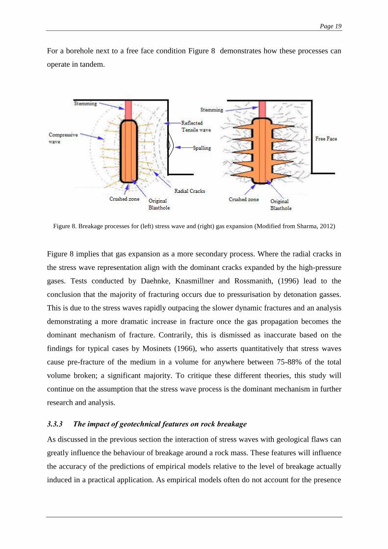
For a borehole next to a free face condition Figure 8 demonstrates how these processes can
operate in tandem.
Figure 8. Breakage processes for (left) stress wave and (right) gas expansion (Modified from Sharma, 2012)
Figure 8 implies that gas expansion as a more secondary process. Where the radial cracks in
the stress wave representation align with the dominant cracks expanded by the high-pressure
gases. Tests conducted by Daehnke, Knasmillner and Rossmanith, (1996) lead to the
conclusion that the majority of fracturing occurs due to pressurisation by detonation gasses.
This is due to the stress waves rapidly outpacing the slower dynamic fractures and an analysis
demonstrating a more dramatic increase in fracture once the gas propagation becomes the
dominant mechanism of fracture. Contrarily, this is dismissed as inaccurate based on the
findings for typical cases by Mosinets (1966), who asserts quantitatively that stress waves
cause pre-fracture of the medium in a volume for anywhere between 75-88% of the total
volume broken; a significant majority. To critique these different theories, this study will
continue on the assumption that the stress wave process is the dominant mechanism in further
research and analysis.
3.3.3 The impact of geotechnical features on rock breakage
As discussed in the previous section the interaction of stress waves with geological flaws can
greatly influence the behaviour of breakage around a rock mass. These features will influence
the accuracy of the predictions of empirical models relative to the level of breakage actually
induced in a practical application. As empirical models often do not account for the presence
Page 20
of geotechnical inconsistencies, it is critical to acknowledge this potential discrepancy. The
following will discuss how these elements affect blast damage envelopes.
The geotechnical heterogeneity of rock caused by joints, faults, dykes, sills bedding planes etc.
is critical to consider in blast design. Singh (2001) goes into further detail to analyse the impact
these geotechnical features have on the success of blasting. Joints can yield impedance
mismatch zones for the influenced rock mass. Shock waves yield higher magnitude attenuation
in jointed media as damping capacity increases with jointing. Any additional fracturing from
gas pressurisation is lost as the joints allow lower resistance pathways for gas to escape which
are then expanded undesirably in the process. If the blasthole itself is intercepted by a major
discontinuity, blasthole cut off can occur.
It is possible for geological intrusions of soft material to impede stress wave propagation as
they transmit lower propagation velocities than the surrounding hard rock mass. The response
in this case will depend on the geometry and composition of the discontinuity. As the
transmission of the stress from and through the joint depends on the incidence angle of the
intercepting stress wave to the joint surface. The attenuation is low if the incidence angle is
approximately parallel or perpendicular but attenuation increases in the range of 15 to 45
degrees. (Singh, 2001) In homogenous layered rock masses, the internal layer thicknesses can
change the way the stress wave is transmitted. Stress waves may also induce vibration initiated
slip along failure planes and can weaken existing cracks through reduction of joint frictional
resistance.
High strength rocks typically contain fewer joints and the cracks will propagate along the path
governed by joints of minimum resistance and maximum shear strength. Essentially, the effect
of major discontinuities can take precedent over the base influence of rock strength. In lower
strength rocks, rock strength will have a relatively greater influence. (Singh, 2001) The
composition of joint fill can influence their strength significantly. Some strong joints may be
filled with calcite while weaker ones may be composed of mud. The joint will have a lesser
negative impact for filling material that has a closer impedance to the main host rock. Clay fill
may contribute to over or under-break. Concurrently small joints with strong fill will influence
overbreak depending more so on joint orientation. The greater the joint aperture the more
Page 21
damaging the impact on blast propagation, while tight joints may have a significantly adverse
impact (Singh, 2001). Also for weaker planes, the more proximal they are to a borehole the
greater the effect on the stress transmission. Intersecting layers of soft material will also inhibit
the consistency of pressure distribution from blasting through the rock mass. The presence of
water can reduce the tensile and compressive strengths of rocks by reducing friction between
particles and asperities of joints. This in turn reduces the cohesion. It may reduce shock wave
attenuation and by extension increase breakage. If a significant volume of water has intruded
into a joint should the rock mass may begin to deform in a tensile capacity, the free water may
form a wedge. (Singh, 2001) The practical tests conducted by Singh (2001) justified that
spacing, width and geometry of discontinuities can significantly influence the transmission of
stress waves in a rock mass. Joints can influence the attenuation of the stress waves. Orientation
and frequency of the joints will also be critical to the propagation of the damage induced by
the blast. In layered rock masses, softer layers more significantly interfere with stress
transference into the rock mass. Damage yielded by blasting is cumulative and previous blasts
may generate new structural planes of weakness beyond what has been designed. (Singh, 2001)
From this collection of observations, it is justifiable to state that the geotechnical structures
will have a significant impact on the outcome of the blast and by extension the accuracy of the
iDamage model. Hence the model is limited in this capacity.
3.4 EXISTING EMPIRICAL BLAST DAMAGE MODELS
Blast damage models are typically predicated on one of two critical parameters being PPV or
pressure. Typically, PPV can be quantified non-invasively and may be used to establish damage
criterion for distant structures. However, the complicated behaviour of vibration in the near
and far field can be a source of difficulty. (Sun, 2013) Several estimates of PPV damage have
been demonstrated in Appendix B. These PPV envelopes establish typical levels of breakage
for rocks of various categorical strengths and may be helpful when interpreting the levels of
breakage associated with PPV dependent empirical models. Using pressure as a basis to
estimate the extent of damage is generally less complicated.
One of the major research objectives was to formulate a review of existing blast damage
models. This will be necessary to permit any comparison of the iDamage model to previously
defined predictive models. This component will quantify the input parameters and critical
functions of the existing models. The existing blast damage models have been identified in
Table 2.
Page 22
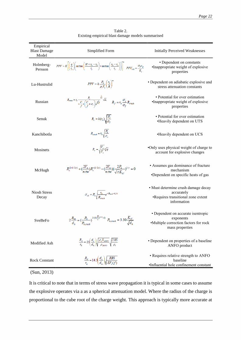
Table 2.
Existing empirical blast damage models summarised
Empirical
Blast Damage
Model
Simplified Form Initially Perceived Weaknesses
Holmberg-
Persson
• Dependent on constants
•Inappropriate weight of explosive
properties
Lu-Hustrulid
• Dependent on adiabatic explosive and
stress attenuation constants
Russian
• Potential for over estimation
•Inappropriate weight of explosive
properties
Senuk
• Potential for over estimation
•Heavily dependent on UTS
Kanchibotla
•Heavily dependent on UCS
Mosinets
•Only uses physical weight of charge to
account for explosive changes
McHugh
• Assumes gas dominance of fracture
mechanism
•Dependent on specific heats of gas
Niosh Stress
Decay
• Must determine crush damage decay
accurately
•Requires transitional zone extent
information
SveBeFo
• Dependent on accurate isentropic
exponents
•Multiple correction factors for rock
mass properties
Modified Ash
• Dependent on properties of a baseline
ANFO product
Rock Constant
• Requires relative strength to ANFO
baseline
•Influential hole confinement constant
(Sun, 2013)
It is critical to note that in terms of stress wave propagation it is typical in some cases to assume
the explosive operates via a as a spherical attenuation model. Where the radius of the charge is
proportional to the cube root of the charge weight. This approach is typically more accurate at
Page 23
ranges more proximal to the charge but yields weaker correlations at greater distances
(Erickson, 2014).
The time constraints of this research project will not permit a comparison to all the indicated
models in Table 2. as well as an effective sensitivity analysis. Concurrently four models have
been isolated for comparison to the iDamage model, they include the:
Holmberg-Persson method;
Lu-Hustrulid method;
Russian method; and the
Senuk method.
(Sun, 2013)
The summaries for these methods will detail how the damage distance is determined and the
component parameters used to arrive at this value.
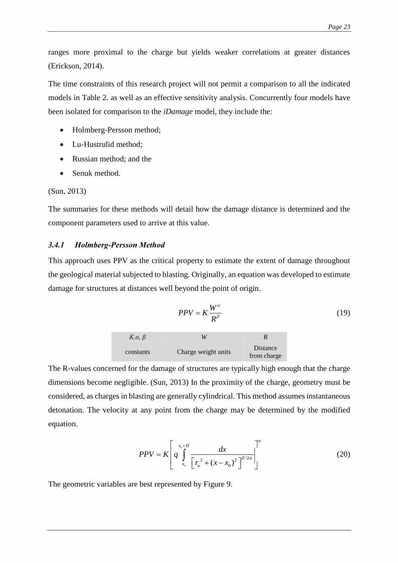
3.4.1 Holmberg-Persson Method
This approach uses PPV as the critical property to estimate the extent of damage throughout
the geological material subjected to blasting. Originally, an equation was developed to estimate
damage for structures at distances well beyond the point of origin.
W
PPV KR
(19)
K,α, β W R
constants Charge weight units Distance
from charge
The R-values concerned for the damage of structures are typically high enough that the charge
dimensions become negligible. (Sun, 2013) In the proximity of the charge, geometry must be
considered, as charges in blasting are generally cylindrical. This method assumes instantaneous
detonation. The velocity at any point from the charge may be determined by the modified
equation.
/2
2 2
0( )
s
s
x H
x o
dxPPV K q
r x x
(20)
The geometric variables are best represented by Figure 9.
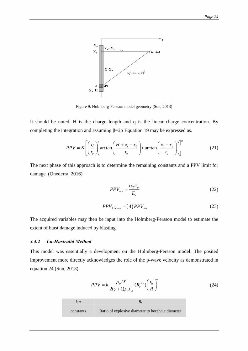
Page 24
Figure 9. Holmberg-Persson model geometry (Sun, 2013)
It should be noted, H is the charge length and q is the linear charge concentration. By
completing the integration and assuming β=2α Equation 19 may be expressed as.
0 0arctan arctans s
o o o
H x x x xqPPV K
r r r
(21)
The next phase of this approach is to determine the remaining constants and a PPV limit for
damage. (Onederra, 2016)
T p
crit
s
cPPV
E
(22)
4fracture critPPV PPV (23)
The acquired variables may then be input into the Holmberg-Persson model to estimate the
extent of blast damage induced by blasting.
3.4.2 Lu-Hustrulid Method
This model was essentially a development on the Holmberg-Persson model. The posited
improvement more directly acknowledges the role of the p-wave velocity as demonstrated in
equation 24 (Sun, 2013)
2
2( )2( 1)
o hr
r p
D rPPV k R
c R
(24)
k,α Rr
constants Ratio of explosive diameter to borehole diameter
Page 25
The formula can be simplified by the inclusion of the borehole pressure. First, the borehole
pressure must be found which is dependent on the detonation pressure.
2
2
CJ eb
h
P dP
d
, where 21
1CJ oP D
(25, 26)
According to Sun, (2013) the Lu-Hustrulid model for PPV can then be expressed as.
b h
r v
P rPPV k
V R
(27)
k,α, γ Ra a R D
constants adiabatic explosive index decoupling
ratio
radius of
charge distance
confined
VOD
It will then be necessary to employ equations 25 and 26 to determine an appropriate value for
the remaining undefined constants.
3.4.3 Russian Method
This approach does not actively require PPV limits to provide a predicted damage radius about
a detonated charge. This method initially dictates it is necessary to identify the crush zone
radius by the following function. The following equations have been summarised by Sun,
(2013).
1
2
1
bcrush b f
f
c
PR r L
C CL
f f
(28)
C L f
cohesion constant Coefficient of friction
Note that f = tan(ϕ), where ϕ is the internal angle of friction and the L is a constant defined by
equation 29.
1 ln
h
cc
T
L r
, where (1 )
sE
(29)
Page 26
The predicted fracture zone is then given by:
cf h crush
T
R r R
(30)
It may be necessary to apply a correction factor in some scenarios. A weakness of this method
is that it reportedly over estimates damage for rocks with a UCS that is less than 100MPa.
(Sun,2013)
3.4.4 Senuk Method
This approach defines a distance of damage for a cylindrical charge using a less extensive
formula. It is not dependent on a PPV of critical fracturing but does require the definition of a
stress concentration factor.
( ) bc h
T
PR k r
(31)
Rc predicts the radius of the crack zone for a cylindrical charge. The stress concentration factor
of k, allows for compensation of stress concentration in cracks and joints. Typically, the value
of this factor is in the range of 1.12 (Sun, 2013). The perceived similarity to the Russian method
may suggest that a correction factor may also be necessary under specific conditions. Critically
though the subjectivity of the application of this factor in different rock materials will have a
significant impact
3.5 CONCLUSION
This literature review has served to identify an effective collection of supporting information
that will be valuable to reinforce the evaluation of the iDamage empirical blast damage model.
Explanation of the behaviour of typical stress waves and the correlation between certain rock
parameters identified many connections between rock parameters. These included σT and UCS,
Poisson’s ratio and s-wave velocity, UCS and p-wave velocity and others. This will supplement
the identified dependencies of the iDamage model as established by the sensitivity analysis
that will be undertaken by this study. The exploration of the explosive detonation practices and
the interaction of stress waves and gaseous expansion to yield rock breakage will also be of
Page 27
merit to consider in this evaluation. As this is the behaviour that the model is attempting to
describe it grounds the empirical predictions in the practical terms and may help identify
limitations of any predictions that may be lower in accuracy. Concurrently, a large component
of this will be the impact of the geotechnical features in a rock mass, which cannot be described
by the input parameters. This affirms the limitations of the model in this capacity. The
exploration of Empirical blast damage models highlighted that there have been numerous
attempts to categorise rock fracture estimates based on rock mass properties and explosive
characteristics. Though the simplicity associated with some of these models results in a
consequent weakness or misrepresentation. By isolating four models to compare the iDamage,
method to an effective scope for comparison could be established. The basis of the Lu-
Hustrulid and Holmberg-Persson models will be representative of models dependent on site-
specific stress attenuation constants, while the Russian and Senuk models are more
fundamentally dependent on rock mass properties. The elaboration on each of these models
was developed to allow any identified inaccuracies under the investigated conditions to be
backtracked and identified. In this case, it would provide support for the use of another model
under the relevant conditions.
Page 28
4. PROJECT METHODLOGY
The importance of adopting an effective strategy at the outset of the project will be closely
correlated to the quality of the associated outcomes and conclusions. The following section
describes the two most critical components involved with management of this research project:
An outline of the strategies used to sufficiently complete the objectives; and
A risk management plan with contingency actions.
This will serve to establish the steps taken to effectively evaluate the iDamage model and
provide the management principles that were pursued to ensure that all necessary tasks were
accomplished as per the initially established aims of the project.
4.1 EVALUATION METHODOLOGY
The methodology adopted will directly reflect the conclusions generated from the analysis of
empirical models and the implications of the approach must be assessed when developing said
conclusions. Once executed any means to develop the methodology further or make
improvements in similar studies in the future will be discussed in the final recommendations
of the project.
4.1.1 Rock mass data and explosive properties determination
In order to develop comparison between the empirical blast damage models identified for the
assessment it was first necessary to establish a range of baseline conditions. These conditions
were defined as the fundamental input parameters for empirical models in terms of both the
rock mass determinants and explosive properties. It was critical that this effectively represented
a broad range of applicable conditions such that any conclusions would be further substantiated
by being representative of a larger sample.
The governing rock properties established included:
UCS;
static tensile strength;
young’s modulus;
rock material density;
p-wave velocities;
Page 29
friction angle; and
cohesion;
To establish a broad range of rock mass values 9 typical rock masses were taken into
consideration. It was necessary to assume that any internal geological inconsistencies not
acknowledged by the input properties were sufficiently negligible. These 9 rock masses were
selected on the basis of generally perceived hardness and were grouped according to UCS. This
categorisation has been demonstrated in Table 3.
Table 3.
Rock mass compressive strength categorisation
Hard Medium Soft
Granite Sandstone Tuff
Basalt Limestone Pegmatite
Gneiss Siltstone Talc Schist
The necessary explosive properties obtained included the:
Velocity of detonation (VOD);
hole diameter;
density;
adiabatic index
Three explosive configurations were selected based on existing characteristics of explosives
used in blasting applications. The explosives to be used in further stages of the evaluation
included:
an ANFO product(VOD = 3600)
a lower yield emulsion (VOD = 4900); and
a higher yield emulsion (VOD = 5500).
These explosive configurations were determined on the basis of having a significant variation
in VOD; and would hence represent a reasonable range of explosive volatility used in practical
scenarios. In summation, the determination of the rock mass properties and explosive
parameters outlined in this methodology will provide a sufficient basis on which to compare
existing empirical blast damage models, develop a sensitivity analysis and ultimately evaluate
the iDamage model.
Page 30
4.1.2 Comparison of empirical blast damage models
The iDamage empirical blast damage model as identified in the literature review will be
compared to a further four blast damage models that are actively utilised. Those models once
more include the:
Holmberg-Persson method;
Lu-Hustrulid method;
Russian method; and the
Senuk method.
(Sun, 2013)
To develop the effective comparison between the methods and the newly developed iDamage
model it will be necessary to develop each combination of variables for the established rock
mass properties and explosive configurations. By contrasting each of the methods against one
another, a context for the outputs of the iDamage model can be established. It is critical to note
however that the Holmberg-Persson and Lu-Hustrulid models were dependent on specific
stress attenuation constants (K, α ). These constants describe the interaction between the
explosive and the rock mass. So a change in either property would result in an uncontrolled
change in the attenuation constants. While this can partially account for the average presence
of regional geological inconsistencies, it can be difficult to obtain them accurately. The
standard method of determination currently involves a log based linear trend from a wide range
of PPV data. An example of such a plot has been provided in Figure 10.
Figure 10. Stress attenuation constant determination (Esen and Onederra, 2004)
The constants are determined from the relationship demonstrated in equation 30.
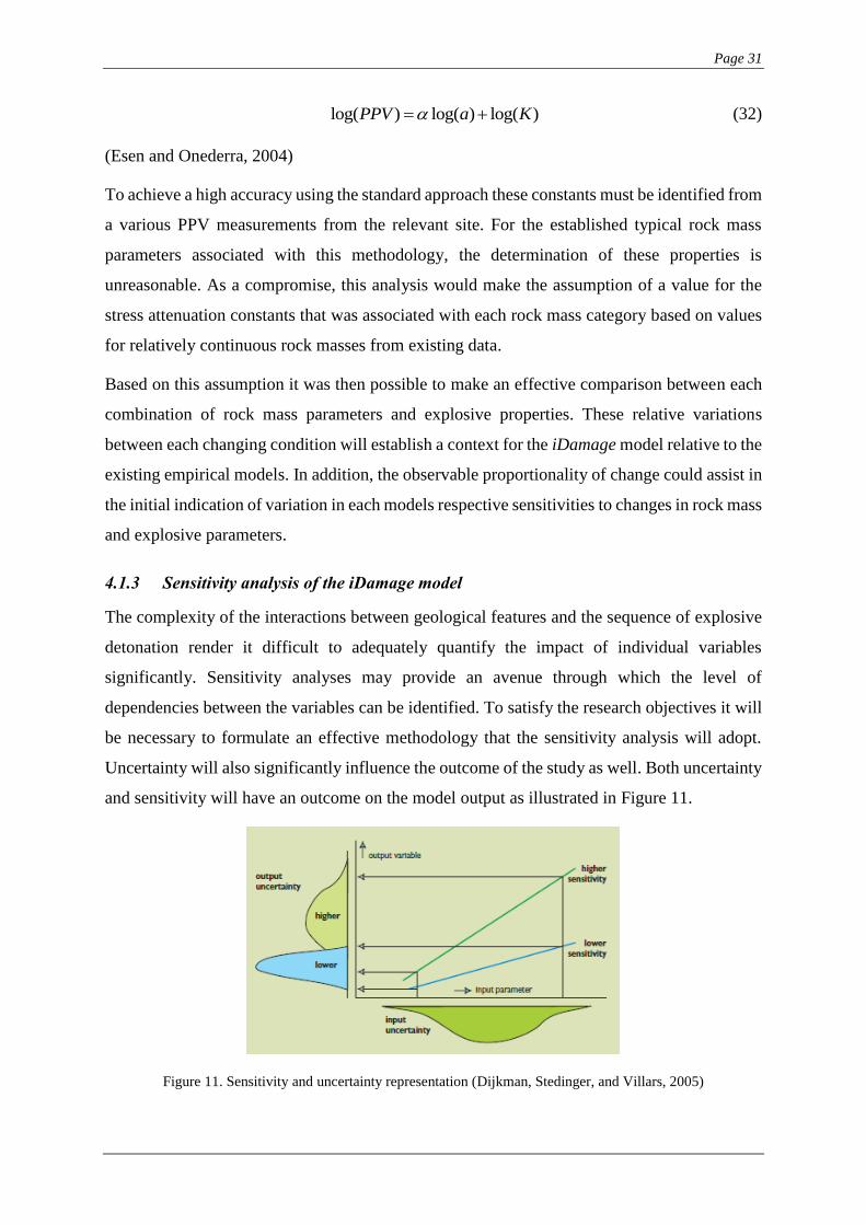
Page 31
log( ) log( ) log( )PPV a K (32)
(Esen and Onederra, 2004)
To achieve a high accuracy using the standard approach these constants must be identified from
a various PPV measurements from the relevant site. For the established typical rock mass
parameters associated with this methodology, the determination of these properties is
unreasonable. As a compromise, this analysis would make the assumption of a value for the
stress attenuation constants that was associated with each rock mass category based on values
for relatively continuous rock masses from existing data.
Based on this assumption it was then possible to make an effective comparison between each
combination of rock mass parameters and explosive properties. These relative variations
between each changing condition will establish a context for the iDamage model relative to the
existing empirical models. In addition, the observable proportionality of change could assist in
the initial indication of variation in each models respective sensitivities to changes in rock mass
and explosive parameters.
4.1.3 Sensitivity analysis of the iDamage model
The complexity of the interactions between geological features and the sequence of explosive
detonation render it difficult to adequately quantify the impact of individual variables
significantly. Sensitivity analyses may provide an avenue through which the level of
dependencies between the variables can be identified. To satisfy the research objectives it will
be necessary to formulate an effective methodology that the sensitivity analysis will adopt.
Uncertainty will also significantly influence the outcome of the study as well. Both uncertainty
and sensitivity will have an outcome on the model output as illustrated in Figure 11.
Figure 11. Sensitivity and uncertainty representation (Dijkman, Stedinger, and Villars, 2005)
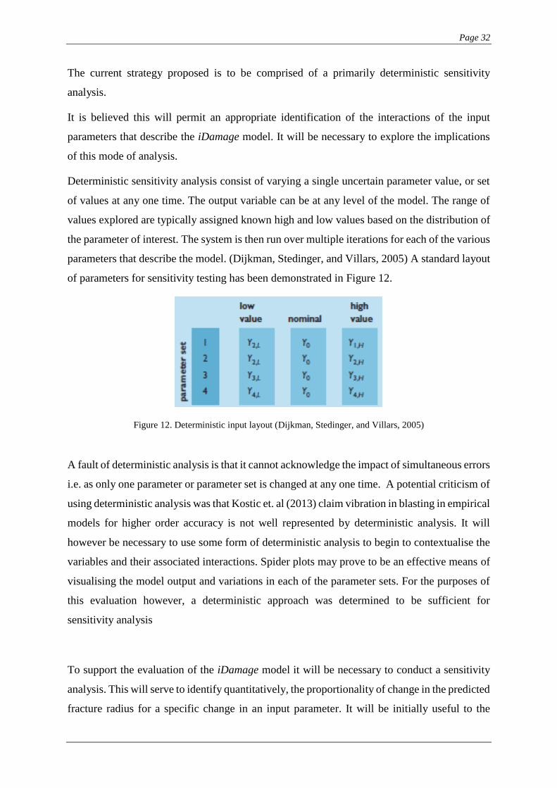
Page 32
The current strategy proposed is to be comprised of a primarily deterministic sensitivity
analysis.
It is believed this will permit an appropriate identification of the interactions of the input
parameters that describe the iDamage model. It will be necessary to explore the implications
of this mode of analysis.
Deterministic sensitivity analysis consist of varying a single uncertain parameter value, or set
of values at any one time. The output variable can be at any level of the model. The range of
values explored are typically assigned known high and low values based on the distribution of
the parameter of interest. The system is then run over multiple iterations for each of the various
parameters that describe the model. (Dijkman, Stedinger, and Villars, 2005) A standard layout
of parameters for sensitivity testing has been demonstrated in Figure 12.
Figure 12. Deterministic input layout (Dijkman, Stedinger, and Villars, 2005)
A fault of deterministic analysis is that it cannot acknowledge the impact of simultaneous errors
i.e. as only one parameter or parameter set is changed at any one time. A potential criticism of
using deterministic analysis was that Kostic et. al (2013) claim vibration in blasting in empirical
models for higher order accuracy is not well represented by deterministic analysis. It will
however be necessary to use some form of deterministic analysis to begin to contextualise the
variables and their associated interactions. Spider plots may prove to be an effective means of
visualising the model output and variations in each of the parameter sets. For the purposes of
this evaluation however, a deterministic approach was determined to be sufficient for
sensitivity analysis
To support the evaluation of the iDamage model it will be necessary to conduct a sensitivity
analysis. This will serve to identify quantitatively, the proportionality of change in the predicted
fracture radius for a specific change in an input parameter. It will be initially useful to the
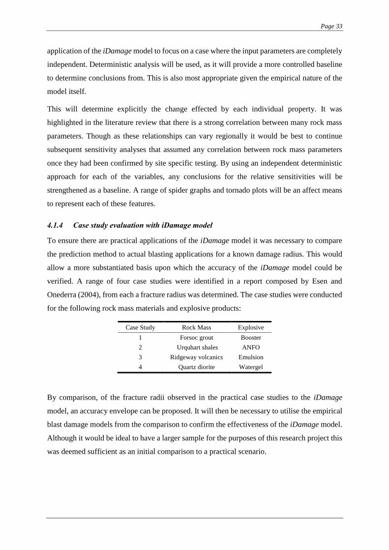
Page 33
application of the iDamage model to focus on a case where the input parameters are completely
independent. Deterministic analysis will be used, as it will provide a more controlled baseline
to determine conclusions from. This is also most appropriate given the empirical nature of the
model itself.
This will determine explicitly the change effected by each individual property. It was
highlighted in the literature review that there is a strong correlation between many rock mass
parameters. Though as these relationships can vary regionally it would be best to continue
subsequent sensitivity analyses that assumed any correlation between rock mass parameters
once they had been confirmed by site specific testing. By using an independent deterministic
approach for each of the variables, any conclusions for the relative sensitivities will be
strengthened as a baseline. A range of spider graphs and tornado plots will be an affect means
to represent each of these features.
4.1.4 Case study evaluation with iDamage model
To ensure there are practical applications of the iDamage model it was necessary to compare
the prediction method to actual blasting applications for a known damage radius. This would
allow a more substantiated basis upon which the accuracy of the iDamage model could be
verified. A range of four case studies were identified in a report composed by Esen and
Onederra (2004), from each a fracture radius was determined. The case studies were conducted
for the following rock mass materials and explosive products:
Case Study Rock Mass Explosive
1 Forsoc grout Booster
2 Urquhart shales ANFO
3 Ridgeway volcanics Emulsion
4 Quartz diorite Watergel
By comparison, of the fracture radii observed in the practical case studies to the iDamage
model, an accuracy envelope can be proposed. It will then be necessary to utilise the empirical
blast damage models from the comparison to confirm the effectiveness of the iDamage model.
Although it would be ideal to have a larger sample for the purposes of this research project this
was deemed sufficient as an initial comparison to a practical scenario.
Page 34
4.1.5 Application of iDamage model to determine blast design parameters
Empirical blast damage models can be used to develop the fundamental input parameters for
the outset of a standard blast design. These parameters include, but are not limited to, burden
and spacing. By having a basis in the behaviour of the rock mass and the associated explosive
agent, it is a better supported foundation upon which to estimate these blast design principles.
Particularly for very early stages in the design process when little is known about the geology
and the response it will yield to an explosive charge. There are some more general methods
that do not factor in the extent of damage into burden estimates. This requires a greater reliance
on general trends or experientially based variations. The burden estimates and spacing will be
determined for the empirical models analysed, these will also be compared against the more
general methods. These general methods include the rules of thumb established by: Dyno
Nobel (2010), Rustan and Kou (1992) as well as the Kostal method assessed by Ahangari and
Shad (2012). These estimates will be provided for both the case study evaluations and the
broad general properties determined from literature. This will offer some context for the blast
design properties obtained from the iDamage model.
4.2 RISK MANAGEMENT
The level of work associated with a research project of this scale will require a more detailed
level of management. To reduce the potentially catastrophic impact of any major setbacks a
risk assessment was conducted in the early phases of this project. The methodology used was
represented by BHP (2009), which involved the use of a severity-probability matrix to rank
threats. Once high threat risks are isolated, the contingency responses can be developed based
on this priority order. The severity and probability criteria established by BHP (2009), have
been modified to more accurately reflect the conditions of this project. Note that the risk
management methodology was reviewed at multiple points throughout the course of the
research project, but as no threats were actualised and no new risks developed the original risk
management strategy was deemed effective for the life of the research project.
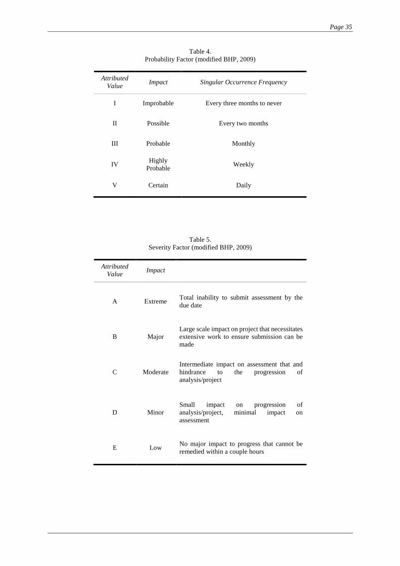
Page 35
Table 4.
Probability Factor (modified BHP, 2009)
Attributed
Value Impact Singular Occurrence Frequency
I Improbable Every three months to never
II Possible Every two months
III Probable Monthly
IV Highly
Probable Weekly
V Certain Daily
Table 5.
Severity Factor (modified BHP, 2009)
Attributed
Value Impact
A Extreme Total inability to submit assessment by the
due date
B Major
Large scale impact on project that necessitates
extensive work to ensure submission can be
made
C Moderate
Intermediate impact on assessment that and
hindrance to the progression of
analysis/project
D Minor
Small impact on progression of
analysis/project, minimal impact on
assessment
E Low No major impact to progress that cannot be
remedied within a couple hours
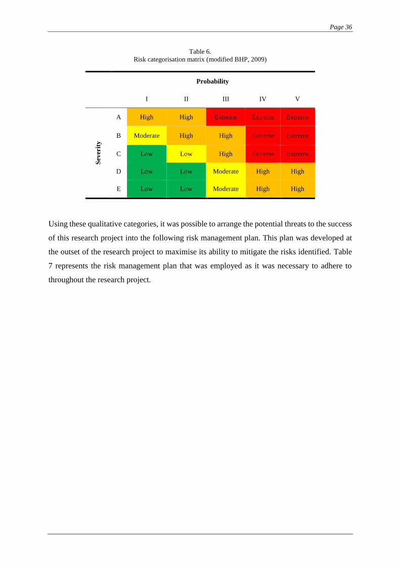
Page 36
Table 6.
Risk categorisation matrix (modified BHP, 2009)
Probability
I II III IV V S
ever
ity
A High High Extreme Extreme Extreme
B Moderate High High Extreme Extreme
C Low Low High Extreme Extreme
D Low Low Moderate High High
E Low Low Moderate High High
Using these qualitative categories, it was possible to arrange the potential threats to the success
of this research project into the following risk management plan. This plan was developed at
the outset of the research project to maximise its ability to mitigate the risks identified. Table
7 represents the risk management plan that was employed as it was necessary to adhere to
throughout the research project.
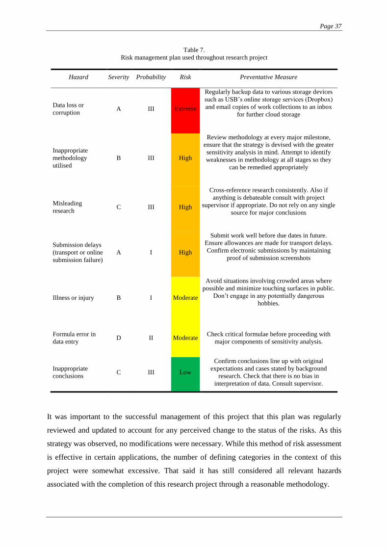
Page 37
Table 7.
Risk management plan used throughout research project
Hazard Severity Probability Risk Preventative Measure
Data loss or
corruption A III Extreme
Regularly backup data to various storage devices
such as USB’s online storage services (Dropbox)
and email copies of work collections to an inbox
for further cloud storage
Inappropriate
methodology
utilised
B III High
Review methodology at every major milestone,
ensure that the strategy is devised with the greater
sensitivity analysis in mind. Attempt to identify
weaknesses in methodology at all stages so they
can be remedied appropriately
Misleading
research C III High
Cross-reference research consistently. Also if
anything is debateable consult with project
supervisor if appropriate. Do not rely on any single
source for major conclusions
Submission delays
(transport or online
submission failure)
A I High
Submit work well before due dates in future.
Ensure allowances are made for transport delays.
Confirm electronic submissions by maintaining
proof of submission screenshots
Illness or injury B I Moderate
Avoid situations involving crowded areas where
possible and minimize touching surfaces in public.
Don’t engage in any potentially dangerous
hobbies.
Formula error in
data entry D II Moderate
Check critical formulae before proceeding with
major components of sensitivity analysis.
Inappropriate
conclusions C III Low
Confirm conclusions line up with original
expectations and cases stated by background
research. Check that there is no bias in
interpretation of data. Consult supervisor.
It was important to the successful management of this project that this plan was regularly
reviewed and updated to account for any perceived change to the status of the risks. As this
strategy was observed, no modifications were necessary. While this method of risk assessment
is effective in certain applications, the number of defining categories in the context of this
project were somewhat excessive. That said it has still considered all relevant hazards
associated with the completion of this research project through a reasonable methodology.
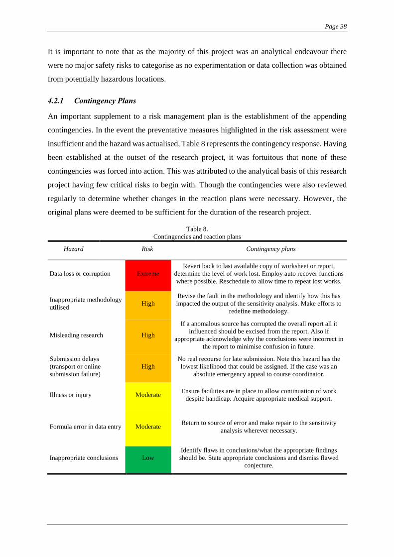
Page 38
It is important to note that as the majority of this project was an analytical endeavour there
were no major safety risks to categorise as no experimentation or data collection was obtained
from potentially hazardous locations.
4.2.1 Contingency Plans
An important supplement to a risk management plan is the establishment of the appending
contingencies. In the event the preventative measures highlighted in the risk assessment were
insufficient and the hazard was actualised, Table 8 represents the contingency response. Having
been established at the outset of the research project, it was fortuitous that none of these
contingencies was forced into action. This was attributed to the analytical basis of this research
project having few critical risks to begin with. Though the contingencies were also reviewed
regularly to determine whether changes in the reaction plans were necessary. However, the
original plans were deemed to be sufficient for the duration of the research project.
Table 8.
Contingencies and reaction plans
Hazard Risk Contingency plans
Data loss or corruption Extreme
Revert back to last available copy of worksheet or report,
determine the level of work lost. Employ auto recover functions
where possible. Reschedule to allow time to repeat lost works.
Inappropriate methodology
utilised High
Revise the fault in the methodology and identify how this has
impacted the output of the sensitivity analysis. Make efforts to
redefine methodology.
Misleading research High
If a anomalous source has corrupted the overall report all it
influenced should be excised from the report. Also if
appropriate acknowledge why the conclusions were incorrect in
the report to minimise confusion in future.
Submission delays
(transport or online
submission failure)
High
No real recourse for late submission. Note this hazard has the
lowest likelihood that could be assigned. If the case was an
absolute emergency appeal to course coordinator.
Illness or injury Moderate Ensure facilities are in place to allow continuation of work
despite handicap. Acquire appropriate medical support.
Formula error in data entry Moderate Return to source of error and make repair to the sensitivity
analysis wherever necessary.
Inappropriate conclusions Low
Identify flaws in conclusions/what the appropriate findings
should be. State appropriate conclusions and dismiss flawed
conjecture.

Page 39
It should be noted that the close conformity to the risk management plan throughout the course
of the research project, effectively mitigated the implications of any risks. Regular review of
these criteria set at the initiation of the project was undertaken to ensure the plans were still up
to date. If this strategy was not adopted the risk management plan may have become outdated
and neglected any new potential threats. Fortunately, though, no new threats were identified
and no major modifications were required of the risk management model. Concurrently this
strategy was also applied to the contingency plans, which also were deemed sufficient
throughout the progression of the project.
4.3 EVALUATION OF PROJECT MANAGEMENT
The lack of actualised risks has permitted this project to be completed in close correlation to
the originally established project plan developed at the outset of the research project. This plan
has been provided in APPENDIX C and has been vital to ensure the execution of all tasks were
completed effectively. To be critical of the plan though, it did not account for other
commitments that would interfere with the completion of certain tasks. Examples of this
included submissions for other course work; this could have been implemented into the project
plan earlier. In addition, a personal commitment that was not integrated into the project plan
disrupted work efforts leading up to the seminar presentation. While this offset the plan by at
most, no more than a few days, the time allocated to each task was sufficient to act as a buffer
to the shock of any unquantified intervention.
The project plan used to ensure the success of the project severed as a set of effective guiding
principles to ensure each component task and sub-critical task was completed. It will be
necessary to continue close adherence to this plan to ensure that the conference paper and
revised thesis submission will be completed effectively.
Page 40
5. COMPARISON OF EMPIRICAL MODELS AND
SENSITIVITY OF THE iDAMAGE MODEL
5.1 INTRODUCTION
The iDamage model has been developed with the intent to provide another means of
developing an initial estimate for the radius of damage on the condition of having access to
basic information. This core information is comprised of the more fundamental characteristics
of the rock mass and parameters describing the composition of the explosive agent to be
employed. To facilitate a detailed evaluation of the iDamage model it will be necessary to
establish:
a comparison to a range of existing empirical models; and
a sensitivity analysis of the input parameters for the iDamage model.
This will be applied over a broad range of rock mass properties and explosive configurations.
The multiple combinations represented by the utilisation of these varied parameters will
generate a wide perspective. By extension, allowing the identification of an extensive
representation of the behaviour of the empirical models and a substantiated sensitivity analysis
specifically for the iDamage model.
5.2 COMPARISON OF EMPIRICAL MODEL PREDICTIONS
The first component in the evaluation of the iDamage model was to determine a selection of
rock mass and explosive properties that was acceptably representative of a broad range of
conditions. This baseline will serve as a strong foundation upon which to understand the
general behaviour of the existing empirical models and contextualise the projections generated
by the iDamage model. With respect to the rock mass properties a total of nine rock masses
were selected for assessment. These were identified categorically by UCS values in being
traditionally defined as either: hard (>130 MPa), medium (70130 MPa) and soft (<70 MPa)
rock masses. Table 9 identifies The properties for each of these rock masses determined from
literature.
Page 41
Table 9.
Fundamental Rock Mass Properties
Sam
ple
Cat
ego
ry
Nam
e
UC
S
(MP
a)
Sta
tic
ten
sile
stre
ng
th
(MP
a)
E
(GP
a)
Den
sity
(t/m
3)
υ
Vp
(m/s
)
α
K
k
Fri
ctio
n A
ng
le
(deg
rees
)
Co
hes
ion
(MP
a)
1 Hard Granite 160 13.33 50 2.75 0.2 6000 0.9 470 1.12 55 45
2 Hard Basalt 165 13.75 48 3.05 0.2 6000 0.9 470 1.12 40 50
3 Hard Andesite 140 11.67 40 3.22 0.2 6150 0.9 470 1.12 40 40
4 Medium Sandstone 105 9.17 35 2.55 0.25 4900 0.95 460 1.12 45 30
5 Medium Gneiss 110 10.83 53 2.9 0.25 5400 0.95 460 1.12 35 25
6 Medium Siltstone 90 7.50 31 2.65 0.25 5200 0.95 460 1.12 25 26
7 Soft Tuff 35 3.00 11.6 1.8 0.3 4650 1.02 456 1.12 15 4.4
8 Soft Pegmatite 65 4.70 20 2.05 0.3 4800 1.02 456 1.12 29 12.9
9 Soft Talc-
Schist 50 4.40 25 2 0.3 5000 1.02 456 1.12 17.5 2.5
(Alvares et al., 2004)
It should be noted that numerous sources were used to verify the baseline input information for
the rock mass data and the specific origins have been detailed in APPENDIX D, Table 29. By
inspection, it can already be identified that there are distinct similarities within each of the
hardness categorisations adopted.
The explosive properties used were isolated to three categories two being emulsions of variable
configurations and the third being a relatively low yield ANFO. This scope of products ought
to give a strong indication as to how variations of explosives are incorporated into blast damage
estimates by empirical models. Table 10 identifies the explicit properties for each of the
explosive configurations considered.
Table 10.
Explosive configuration parameters
Explosive Designation VOD
(m/s)
Density
(t/m3)
adiabatic
index
1 Emulsion A 5500 1.22 3
2 Emulsion B 4900 1.15 3
3 ANFO 3600 1.05 3
(Crowther et al., 1991)
Similar to the rock mass properties, the numerous sources to determine the explosive
parameters have been clarified in
Page 42
Table 30 of APPENDIX D. All trials with the explosive were assumed to take place for a fully
coupled condition for a fully confined blasthole (no nearby faces for wave reflection potential).
The charge length was assumed sufficiently high such that the maximal VOD of the explosive
was achieved in each trial. This is consistent with the model assumptions and limitations. The
K and α constants are stress attenuation constants used by Holmberg-persson and Lu-Hustrulid
methods that describe the interaction between the explosive and the rock mass. To obtain them
accurately PPV data must be determined from vibration recordings. While these in actuality
should change for each combination of explosive and rock mass this would not be feasible
given the demands outlined by the methodology. A simplification was necessary whereby a
baseline set of constants were applied to the rock masses based on their classification as either
hard, medium or soft. It is by this logic that the constants have been associated with the
geotechnical rock parameters in Table 9.
With these varied data sets, each empirical strategy can compose each combination of rock
mass parameters and explosive characteristics to determine an estimate for the projected
fracture radius of each set of conditions. A series of borehole diameters were varied for each
trial to allow for a range of comparisons to be made in a relatively succinct capacity. Table 32
through to Table 34 of APPENDIX D, provide the determined fracture radii for each empirical
model for the controlled set of input parameters. It can be noted there is a general similarity
between each rock mass category by inspection. From this, averaging the predicted damage
into a standard case for hard, medium and soft rock conditions would more effectively facilitate
a comparison between each of the empirical blast damage models. Table 11 represents the
predicted damage radii for the general hard, medium and soft rock categories for each explosive
agent. Despite this combination of data points into average indicative values there still remains
a large set of data to assess. It will be necessary to analyse the data further before relationships
can be identified with any level of certitude
5.2.1 Graphical Analysis of Empirical Comparison
In order to represent this more effectively for each explosive condition the iDamage model will
be compared to each remaining empirical model graphically. Recall that the comparison will
be made on a basis relative to the iDamage model. A a general context for the outputs of the
blast damage model will be established from the use of these plots.
Page 43
Table 11.
Summary of Comparison Results
Emulsion A Emulsion B ANFO
Hard Medium Soft Hard Medium Soft Hard Medium Soft
Em
pri
cal
Mo
del
Bo
reh
ole
Dia
met
er
(mm
)
Dam
age
Ran
ge
(m)
Dam
age
Ran
ge
(m)
Dam
age
Ran
ge
(m)
Dam
age
Ran
ge
(m)
Dam
age
Ran
ge
(m)
Dam
age
Ran
ge
(m)
Dam
age
Ran
ge
(m)
Dam
age
Ran
ge
(m)
Dam
age
Ran
ge
(m)
Lu-Hustrulid 75 2.3 2.7 3.4 1.8 2.1 2.5 0.9 1.2 1.6
Lu-Hustrulid 100 3.0 3.9 4.8 2.2 2.7 3.4 1.2 1.5 1.9
Lu-Hustrulid 120 3.8 4.8 5.6 2.6 3.4 4.4 1.4 1.8 2.1
Lu-Hustrulid 140 4.5 5.4 6.6 3.1 4.1 5.1 1.6 2.0 2.3
Lu-Hustrulid 160 5.1 6.2 7.6 3.7 4.7 5.7 1.8 2.1 2.6
Lu-Hustrulid 180 5.6 7.0 8.8 4.2 5.2 6.4 1.9 2.3 3.0
Lu-Hustrulid 200 6.2 7.9 9.7 4.6 5.7 7.2 2.1 2.5 3.4
Holmberg-Persson 75 0.8 1.2 1.5 0.7 1.1 1.5 0.7 1.0 1.3
Holmberg-Persson 100 1.5 1.9 2.2 1.4 1.8 2.1 1.3 1.7 2.0
Holmberg-Persson 120 1.9 2.4 3.2 1.8 2.3 2.9 1.7 2.1 2.6
Holmberg-Persson 140 2.5 3.4 4.7 2.3 3.1 4.4 2.2 2.8 3.9
Holmberg-Persson 160 3.3 4.6 5.9 3.1 4.3 5.6 2.8 3.9 5.1
Holmberg-Persson 180 4.3 5.6 7.4 4.0 5.3 7.0 3.6 5.0 6.4
Holmberg-Persson 200 5.2 6.9 9.4 4.9 6.5 8.8 4.6 6.0 8.0
iDamage 75 1.8 2.1 3.2 1.6 1.9 3.0 1.0 1.3 2.3
iDamage 100 2.4 2.7 4.5 2.1 2.4 4.1 1.4 1.8 3.1
iDamage 120 2.9 3.3 5.4 2.5 2.9 4.9 1.7 2.1 3.7
iDamage 140 3.4 3.8 6.3 2.9 3.4 5.7 2.0 2.5 4.3
iDamage 160 3.8 4.4 7.1 3.3 3.9 6.5 2.2 2.8 4.9
iDamage 180 4.3 4.9 8.0 3.7 4.4 7.3 2.5 3.1 5.4
iDamage 200 4.7 5.5 8.8 4.1 4.9 8.1 2.8 3.5 6.1
Russian 75 1.8 2.7 4.0 1.7 2.5 3.7 1.2 1.9 3.0
Russian 100 2.4 3.6 5.3 2.3 3.4 4.9 1.5 2.5 4.0
Russian 120 2.9 4.3 6.4 2.7 4.0 5.9 1.9 3.1 4.8
Russian 140 3.4 5.1 7.5 3.2 4.7 6.8 2.2 3.6 5.6
Russian 160 3.9 5.8 8.5 3.6 5.4 7.8 2.5 4.1 6.4
Russian 180 4.4 6.5 9.6 4.1 6.0 8.8 2.8 4.6 7.2
Russian 200 4.9 7.2 10.7 4.5 6.7 9.8 3.1 5.1 8.1
Senuk 75 2.5 3.0 4.9 2.2 2.6 4.2 1.5 1.8 3.0
Senuk 100 3.4 4.0 6.5 2.9 3.5 5.6 2.0 2.4 3.9
Senuk 120 4.0 4.8 7.8 3.5 4.2 6.7 2.4 2.9 4.7
Senuk 140 4.7 5.6 9.1 4.1 4.9 7.9 2.9 3.4 5.5
Senuk 160 5.4 6.4 10.4 4.6 5.5 9.0 3.3 3.9 6.3
Senuk 180 6.0 7.2 11.7 5.2 6.2 10.1 3.7 4.4 7.1
Senuk 200 6.7 8.0 13.0 5.8 6.9 11.2 4.1 4.9 7.9
Page 44
Figure 13. Comparison of Lu-Hustrulid to iDamage model - Emulsion A
Figure 14. Comparison of Lu-Hustrulid to iDamage model - Emulsion B
0
1
2
3
4
5
6
7
8
9
10
11
40 60 80 100 120 140 160 180 200 220
Max
imu
m P
red
icte
d f
ract
ure
rad
ius
(m)
Charge diameter (mm)
Empirical Model Comparison (Emulsion A): Lu-Hustrulid
Lu-Hustrulid: Hard
Lu-Hustrulid:Medium
Lu-Hustrulid: Soft
iDamage: Hard
iDamage: Medium
iDamage: Soft
0
0.5
1
1.5
2
2.5
3
3.5
4
4.5
5
5.5
6
6.5
7
7.5
8
8.5
40 60 80 100 120 140 160 180 200 220
Max
imu
m P
red
icte
d f
ract
ure
rad
ius
(m)
Charge diameter (mm)
Empirical Model Comparison (Emulsion B): Lu-Hustrulid
Lu-Hustrulid: Hard
Lu-Hustrulid:Medium
Lu-Hustrulid: Soft
iDamage: Hard
iDamage: Medium
iDamage: Soft
Page 45
Figure 15. Comparison of Lu-Hustrulid to iDamage model - ANFO
In each case for the combinations between the rock mass parameters and the explosive
characteristics there is a noticeable disparity. The most apparent observations from the
comparison of the iDamage model to the Lu-Hustrulid model for common inputs include:
for emulsion A, the Lu-Hustrulid yields consistently larger estimates than iDamage,
more noticeably for medium and hard rock;
for emulsion B, the Lu-Hustrulid model relative to the iDamage model has decreased
by a greater value. Suggests a greater than proportionate decrease in the predicted
damage as a result of the decrease in capability of the explosive;
for emulsion B Lu-Hustrulid displays slightly more damage (difference of < 1m) for
hard and medium rock masses and reports a lower damage envelope for soft rock
relative to iDamage model;
for ANFO drastic reduction in Lu-Hustrulid output. Much greater than proportional
decrease in damage estimate relative to the decrease in the iDamage model.
The major inferences that can be made from these observations for each of these cases are that
Lu-Hustrulid decreases more significantly with decreasing explosive volatility. Also that the
iDamage model demonstrates a more measured variation in damage estimates for each case.
0
0.5
1
1.5
2
2.5
3
3.5
4
4.5
5
5.5
6
6.5
40 60 80 100 120 140 160 180 200 220
Max
imu
m P
red
icte
d f
ract
ure
rad
ius
(m)
Charge diameter (mm)
Empirical Model Comparison (ANFO): Lu-Hustrulid
Lu-Hustrulid: Hard
Lu-Hustrulid:Medium
Lu-Hustrulid: Soft
Onederra (2016):Hard
Onederra (2016):Medium
Onederra (2016):Soft
Page 46
Figure 16. Comparison of Holmberg-Persson to iDamage model - Emulsion A
Figure 17. Comparison of Holmberg-Persson to iDamage model - Emulsion B
0
1
2
3
4
5
6
7
8
9
10
40 60 80 100 120 140 160 180 200 220
Max
imu
m P
red
icte
d f
ract
ure
rad
ius
(m)
Charge diameter (mm)
Empirical Model Comparison (Emulsion A): Holmberg-Persson
Holmberg-Persson:Hard
Holmberg-Persson:Medium
Holmberg-Persson:Soft
iDamage: Hard
iDamage: Medium
iDamage: Soft
0
1
2
3
4
5
6
7
8
9
10
40 60 80 100 120 140 160 180 200 220
Max
imu
m P
red
icte
d f
ract
ure
rad
ius
(m)
Charge diameter (mm)
Empirical Model Comparison (Emulsion B): Holmberg-Persson
Holmberg-Persson:Hard
Holmberg-Persson:Medium
Holmberg-Persson:Soft
iDamage: Hard
iDamage: Medium
iDamage: Soft
Page 47
Figure 18. Comparison of Holmberg-Persson to iDamage model - ANFO
For the Comparison to the Holmberg-Persson model several observations were established:
for the Holmberg-Persson model with emulsion A, the change in fracture radius is linear
up until a charge diameter of approximately 120mm at which point the proportional
increase in damage increases drastically. Generally offering a much lower estimate than
the iDamage model
for emulsion B, the Holmberg-Persson model demonstrated the same trend. Predicting
a low damage radius to approximately 120mm before increasing significantly. The
order of proportionality between hard medium and soft rock masses were similar to
those of emulsion A;
expectedly for ANFO the trend held once more with very little variation in damage
estimates from those that used far more volatile explosives.
It can be discerned that for each explosive variation the HP model offers little change in damage
estimates for each rock type. While this was more prominent in softer rocks, it is clear that the
iDamage model reflects the change in the explosive to a greater extent. It also would seem that
the HP model could only appropriate changes in the rock mass at high borehole diameters as
well, where low borehole diameters offer relatively lesser variation in estimated fracture radii.
0
1
2
3
4
5
6
7
8
9
40 60 80 100 120 140 160 180 200 220
Max
imu
m P
red
icte
d f
ract
ure
rad
ius
(m)
Charge diameter (mm)
Empirical Model Comparison (ANFO): Holmberg-Persson
Holmberg-Persson:Hard
Holmberg-Persson:Medium
Holmberg-Persson:Soft
iDamage: Hard
iDamage: Medium
iDamage: Soft
Page 48
Figure 19. Comparison of Russian model to iDamage model - Emulsion A
Figure 20. Comparison of Russian model to iDamage model - Emulsion B
0.0
1.0
2.0
3.0
4.0
5.0
6.0
7.0
8.0
9.0
10.0
11.0
12.0
40 60 80 100 120 140 160 180 200 220
Max
imu
m P
red
icte
d f
ract
ure
rad
ius
(m)
Charge diameter (mm)
Empirical Model Comparison (Emulsion A): Russian
iDamage: Hard
iDamage: Medium
iDamage: Soft
Russian: Hard
Russian: Medium
Russian: Soft
0.0
1.0
2.0
3.0
4.0
5.0
6.0
7.0
8.0
9.0
10.0
11.0
40 60 80 100 120 140 160 180 200 220
Max
imu
m P
red
icte
d f
ract
ure
rad
ius
(m)
Charge diameter (mm)
Empirical Model Comparison (Emulsion B): Russian
iDamage: Hard
iDamage: Medium
iDamage: Soft
Russian: Hard
Russian: Medium
Russian: Soft
Page 49
Figure 21. Comparison of Russian model to iDamage model - ANFO
When making comparisons between the iDamage model and the Russian model for each
variation in explosive volatility across the range of rock masses the observations were relatively
more apparent. Whereby:
in the case of emulsion A, there was a strong correlation for the hard rock mass between
the iDamage model and the Russian model. This correlation deteriorated for lower rock
competencies. The Russian estimate for medium strength rock was more proximal to
the iDamage estimate for soft and the Russian soft rock estimate was higher;
the same trend pervaded through the emulsion B scenario. Though the correlation was
not as close for hard rock as it was for emulsion A;
the ANFO trial also resulted in consistent over estimation of the Russian method
relative to the iDamage model.
It would appear that the Russian method is most applicable to materials belonging to the hard
rock category. In relatively softer materials, there is a strong tendency for over estimation
relative to the iDamage model and the estimates of the Lu-Hustrulid and Holmberg-Persson
models. Like the iDamage model a strong linear trend for an increase in explosive diameter is
yielded by the Russian model
0.0
1.0
2.0
3.0
4.0
5.0
6.0
7.0
8.0
9.0
40 60 80 100 120 140 160 180 200 220
Max
imu
m P
red
icte
d f
ract
ure
rad
ius
(m)
Charge diameter (mm)
Empirical Model Comparison (ANFO): Russian
iDamage: Hard
iDamage: Medium
iDamage: Soft
Russian: Hard
Russian: Medium
Russian: Soft
Page 50
Figure 22. Comparison of Senuk model to iDamage model - Emulsion A
Figure 23. . Comparison of Senuk model to iDamage model - Emulsion B
0.0
1.0
2.0
3.0
4.0
5.0
6.0
7.0
8.0
9.0
10.0
11.0
12.0
13.0
14.0
40 60 80 100 120 140 160 180 200 220
Max
imu
m P
red
icte
d f
ract
ure
rad
ius
(m)
Charge diameter (mm)
Empirical Model Comparison (Emulsion A): Senuk
iDamage: Hard
iDamage: Medium
iDamage: Soft
Senuk: Hard
Senuk: Medium
Senuk: Soft
0.0
1.0
2.0
3.0
4.0
5.0
6.0
7.0
8.0
9.0
10.0
11.0
12.0
40 60 80 100 120 140 160 180 200 220
Max
imu
m P
red
icte
d f
ract
ure
rad
ius
(m)
Charge diameter (mm)
Empirical Model Comparison (Emulsion B): Senuk
iDamage: Hard
iDamage: Medium
iDamage: Soft
Senuk: Hard
Senuk: Medium
Senuk: Soft
Page 51
Figure 24. . Comparison of Senuk model to iDamage model - ANFO
For the assessment of the Senuk model in contrast to the iDamage model it was determined to
be quite similar in behaviour to the Russian model. Where it was observed:
there was a tendency to conform to a positive linear relationship between the charge
diameter and damage projected. Also the Senuk model reported a value consistently
larger than the iDamage model. The capacity of this was observed to increase as the
rock mass quality deteriorated from hard to soft;
the changes in explosive condition are appropriated by the Senuk model in some
capacity but particularly for the emulsion cases the soft rock estimates were relatively
much higher than those identified by the iDamage or other models; and
the level of over estimation decreased as the volatility of the explosive decreased as
well.
The Senuk model shared many similarities with the Russian model but as a result of its
simplicity would have a relatively limited application due to the magnitude and persistence of
over estimation. Though this simplicity may have novel applications where there may be a
specific set of conditions for which the model can effectively be utilised.
0.0
1.0
2.0
3.0
4.0
5.0
6.0
7.0
8.0
9.0
40 60 80 100 120 140 160 180 200 220
Max
imu
m P
red
icte
d f
ract
ure
rad
ius
(m)
Charge diameter (mm)
Empirical Model Comparison( ANFO): Senuk
iDamage: Hard
iDamage: Medium
iDamage: Soft
Senuk: Hard
Senuk: Medium
Senuk: Soft
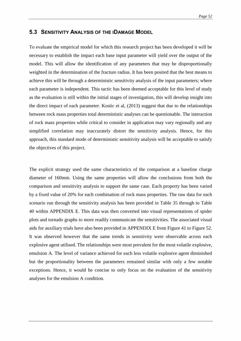
Page 52
5.3 SENSITIVITY ANALYSIS OF THE IDAMAGE MODEL
To evaluate the empirical model for which this research project has been developed it will be
necessary to establish the impact each base input parameter will yield over the output of the
model. This will allow the identification of any parameters that may be disproportionally
weighted in the determination of the fracture radius. It has been posited that the best means to
achieve this will be through a deterministic sensitivity analysis of the input parameters; where
each parameter is independent. This tactic has been deemed acceptable for this level of study
as the evaluation is still within the initial stages of investigation, this will develop insight into
the direct impact of each parameter. Kostic et al, (2013) suggest that due to the relationships
between rock mass properties total deterministic analyses can be questionable. The interaction
of rock mass properties while critical to consider in application may vary regionally and any
simplified correlation may inaccurately distort the sensitivity analysis. Hence, for this
approach, this standard mode of deterministic sensitivity analysis will be acceptable to satisfy
the objectives of this project.
The explicit strategy used the same characteristics of the comparison at a baseline charge
diameter of 160mm. Using the same properties will allow the conclusions from both the
comparison and sensitivity analysis to support the same case. Each property has been varied
by a fixed value of 20% for each combination of rock mass properties. The raw data for each
scenario run through the sensitivity analysis has been provided in Table 35 through to Table
40 within APPENDIX E. This data was then converted into visual representations of spider
plots and tornado graphs to more readily communicate the sensitivities. The associated visual
aids for auxiliary trials have also been provided in APPENDIX E from Figure 41 to Figure 52.
It was observed however that the same trends in sensitivity were observable across each
explosive agent utilised. The relationships were most prevalent for the most volatile explosive,
emulsion A. The level of variance achieved for each less volatile explosive agent diminished
but the proportionality between the parameters remained similar with only a few notable
exceptions. Hence, it would be concise to only focus on the evaluation of the sensitivity
analyses for the emulsion A condition.
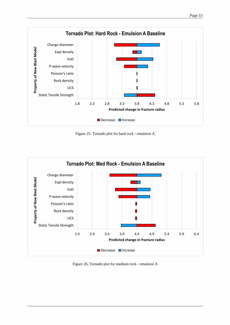
Page 53
Figure 25. Tornado plot for hard rock - emulsion A
Figure 26. Tornado plot for medium rock - emulsion A
1.8 2.3 2.8 3.3 3.8 4.3 4.8 5.3 5.8
Static Tensile Strength
UCS
Rock density
Poisson's ratio
P-wave velocity
VoD
Expl density
Charge diameter
Predicted change in fracture radius
Pro
pe
rty
of
Ne
w B
last
Mo
de
lTornado Plot: Hard Rock - Emulsion A Baseline
Decrease Increase
2.4 2.9 3.4 3.9 4.4 4.9 5.4 5.9 6.4
Static Tensile Strength
UCS
Rock density
Poisson's ratio
P-wave velocity
VoD
Expl density
Charge diameter
Predicted change in fracture radius
Pro
pe
rty
of
Ne
w B
last
Mo
de
l
Tornado Plot: Med Rock - Emulsion A Baseline
Decrease Increase
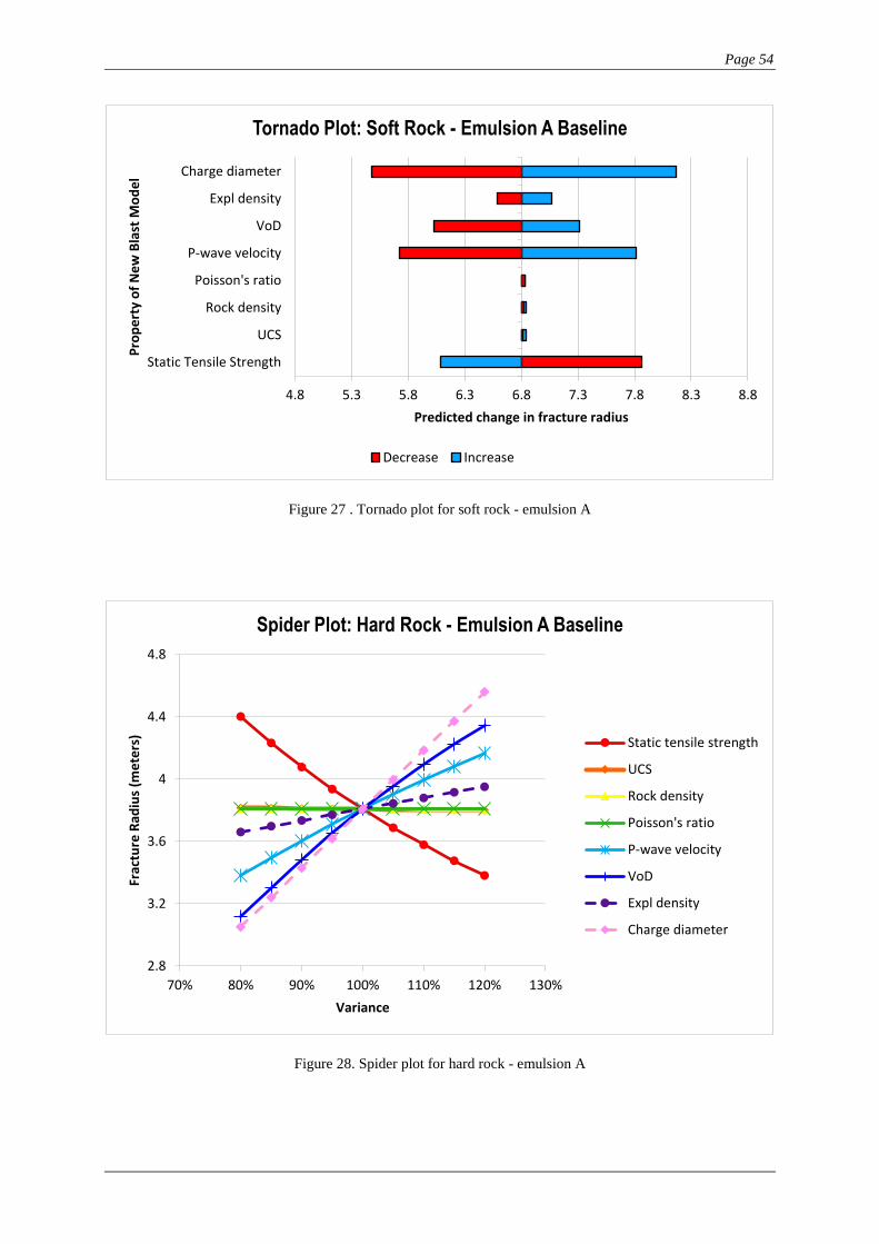
Page 54
Figure 27 . Tornado plot for soft rock - emulsion A
Figure 28. Spider plot for hard rock - emulsion A
4.8 5.3 5.8 6.3 6.8 7.3 7.8 8.3 8.8
Static Tensile Strength
UCS
Rock density
Poisson's ratio
P-wave velocity
VoD
Expl density
Charge diameter
Predicted change in fracture radius
Pro
pe
rty
of
Ne
w B
last
Mo
de
lTornado Plot: Soft Rock - Emulsion A Baseline
Decrease Increase
2.8
3.2
3.6
4
4.4
4.8
70% 80% 90% 100% 110% 120% 130%
Frac
ture
Rad
ius
(me
ters
)
Variance
Spider Plot: Hard Rock - Emulsion A Baseline
Static tensile strength
UCS
Rock density
Poisson's ratio
P-wave velocity
VoD
Expl density
Charge diameter
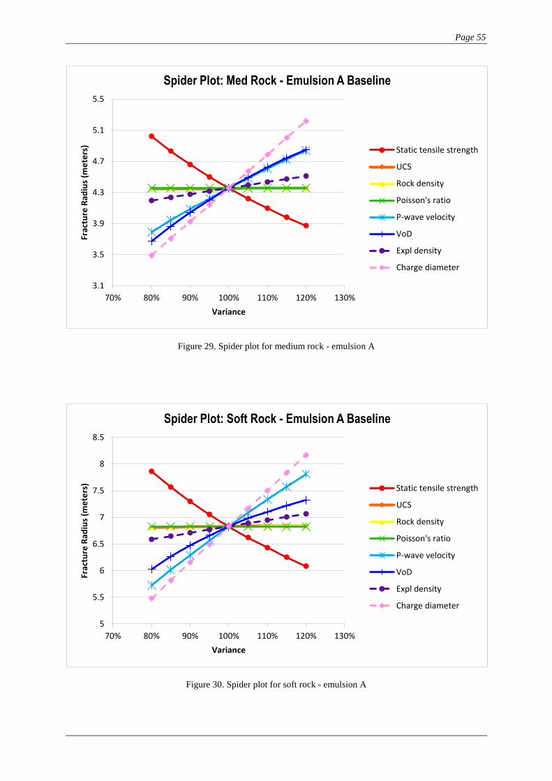
Page 55
Figure 29. Spider plot for medium rock - emulsion A
Figure 30. Spider plot for soft rock - emulsion A
3.1
3.5
3.9
4.3
4.7
5.1
5.5
70% 80% 90% 100% 110% 120% 130%
Frac
ture
Rad
ius
(me
ters
)
Variance
Spider Plot: Med Rock - Emulsion A Baseline
Static tensile strength
UCS
Rock density
Poisson's ratio
P-wave velocity
VoD
Expl density
Charge diameter
5
5.5
6
6.5
7
7.5
8
8.5
70% 80% 90% 100% 110% 120% 130%
Frac
ture
Rad
ius
(me
ters
)
Variance
Spider Plot: Soft Rock - Emulsion A Baseline
Static tensile strength
UCS
Rock density
Poisson's ratio
P-wave velocity
VoD
Expl density
Charge diameter
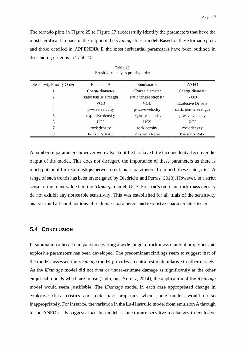
Page 56
The tornado plots in Figure 25 to Figure 27 successfully identify the parameters that have the
most significant impact on the output of the iDamage blast model. Based on these tornado plots
and those detailed in APPENDIX E the most influential parameters have been outlined in
descending order as in Table 12
Table 12.
Sensitivity analysis priority order
Sensitivity Priority Order Emulsion A Emulsion B ANFO
1 Charge diameter Charge diameter Charge diameter
2 static tensile strength static tensile strength VOD
3 VOD VOD Explosive Density
4 p-wave velocity p-wave velocity static tensile strength
5 explosive density explosive density p-wave velocity
6 UCS UCS UCS
7 rock density rock density rock density
8 Poisson’s Ratio Poisson’s Ratio Poisson’s Ratio
A number of parameters however were also identified to have little independent affect over the
output of the model. This does not disregard the importance of these parameters as there is
much potential for relationships between rock mass parameters from both these categories. A
range of such trends has been investigated by Diedrichs and Perras (2013). However, in a strict
sense of the input value into the iDamage model, UCS, Poisson’s ratio and rock mass density
do not exhibit any noticeable sensitivity. This was established for all trials of the sensitivity
analysis and all combinations of rock mass parameters and explosive characteristics tested.
5.4 CONCLUSION
In summation a broad comparison covering a wide range of rock mass material properties and
explosive parameters has been developed. The predominant findings seem to suggest that of
the models assessed the iDamage model provides a central estimate relative to other models.
As the iDamage model did not over or under-estimate damage as significantly as the other
empirical models which are in use (Unlu, and Yilmaz, 2014), the application of the iDamage
model would seem justifiable. The iDamage model in each case appropriated change in
explosive characteristics and rock mass properties where some models would do so
inappropriately. For instance, the variation in the Lu-Hustrulid model from emulsion A through
to the ANFO trials suggests that the model is much more sensitive to changes in explosive
Page 57
parameters. Contrarily the variations in fracture radii from the Holmberg-Persson model did
not vary significantly, as the type of explosive was changed suggesting a lack of sensitivity to
explosive parameters. The Russian and Senuk models consistently overestimated the blast
damage envelope. This may be a result of there being an excessive empirical weight on the
tensile strength of the rock mass. If the iDamage model posited consistently higher or lower
results than all models assessed there would be a basis to question its applicability. However,
it aligned more centrally to predicted damage radii from the remaining empirical methods. This
serves to establish the context of the iDamage model being well within the damage projections
of other empirical blast damage models and supports the use of the model more frequently in
practical applications
The generated spider plots in Figure 28 through to Figure 30 support this priority order of
influence established for the input parameters. As it is clear that the gradients for the most
influential parameters are among the highest on each respective plot. The priority order remains
the same across each variation of rock mass properties with one exception. This exception was
also identified for the alternate explosive configuration baselines plotted in APPENDIX E. The
sensitivity associated with the p-wave velocity increases in magnitude as the quality of the rock
mass deteriorates. Relative to the sensitivity of the less active parameters and the VOD it is
clear that the sensitivity of p-wave velocity has increased. While this is most notable when
contrasting the hard and soft rock conditions, the medium rock state justifies this relationship
by serving as an intermediary value between the two. From the Spider plots identified in
APPENDIX E it is apparent that as the volatility of the explosive baseline decreases the
sensitivity of explosive density relative to other parameters increases. Whereby it is relatively
higher for emulsion B and more so for ANFO. In addition, the influence of VOD on the low
yield ANFO was relatively much more significant than in the emulsion scenarios. It is
noteworthy that the iDamage model is most dependent on a variety of parameters that describe
both the rock mass and explosive characteristics for Emulsion A and B. For the lower yield
ANFO however the explosive properties generally effect the most significant influence over
the output for estimated fracture radius. The general variance in each case supported the claims
for priority order of the input parameters. If there were more time and resources to develop this
sensitivity analysis, it would be ideal to investigate some situations of co-dependence between
input parameters based on some known site data. Also from this a stochastic based analysis
could be established which would advance the deterministic findings at this level.
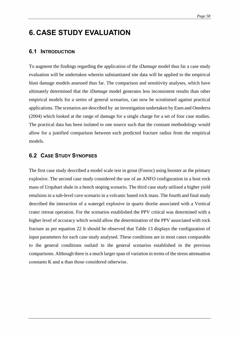
Page 58
6. CASE STUDY EVALUATION
6.1 INTRODUCTION
To augment the findings regarding the application of the iDamage model thus far a case study
evaluation will be undertaken wherein substantiated site data will be applied to the empirical
blast damage models assessed thus far. The comparison and sensitivity analyses, which have
ultimately determined that the iDamage model generates less inconsistent results than other
empirical models for a series of general scenarios, can now be scrutinised against practical
applications. The scenarios are described by an investigation undertaken by Esen and Onederra
(2004) which looked at the range of damage for a single charge for a set of four case studies.
The practical data has been isolated to one source such that the constant methodology would
allow for a justified comparison between each predicted fracture radius from the empirical
models.
6.2 CASE STUDY SYNOPSES
The first case study described a model scale test in grout (Fosroc) using booster as the primary
explosive. The second case study considered the use of an ANFO configuration in a host rock
mass of Urquhart shale in a bench stoping scenario. The third case study utilised a higher yield
emulsion in a sub-level cave scenario in a volcanic based rock mass. The fourth and final study
described the interaction of a watergel explosive in quartz diorite associated with a Vertical
crater retreat operation. For the scenarios established the PPV critical was determined with a
higher level of accuracy which would allow the determination of the PPV associated with rock
fracture as per equation 22 It should be observed that Table 13 displays the configuration of
input parameters for each case study analysed. These conditions are in most cases comparable
to the general conditions outlaid in the general scenarios established in the previous
comparisons. Although there is a much larger span of variation in terms of the stress attenuation
constants K and α than those considered otherwise.
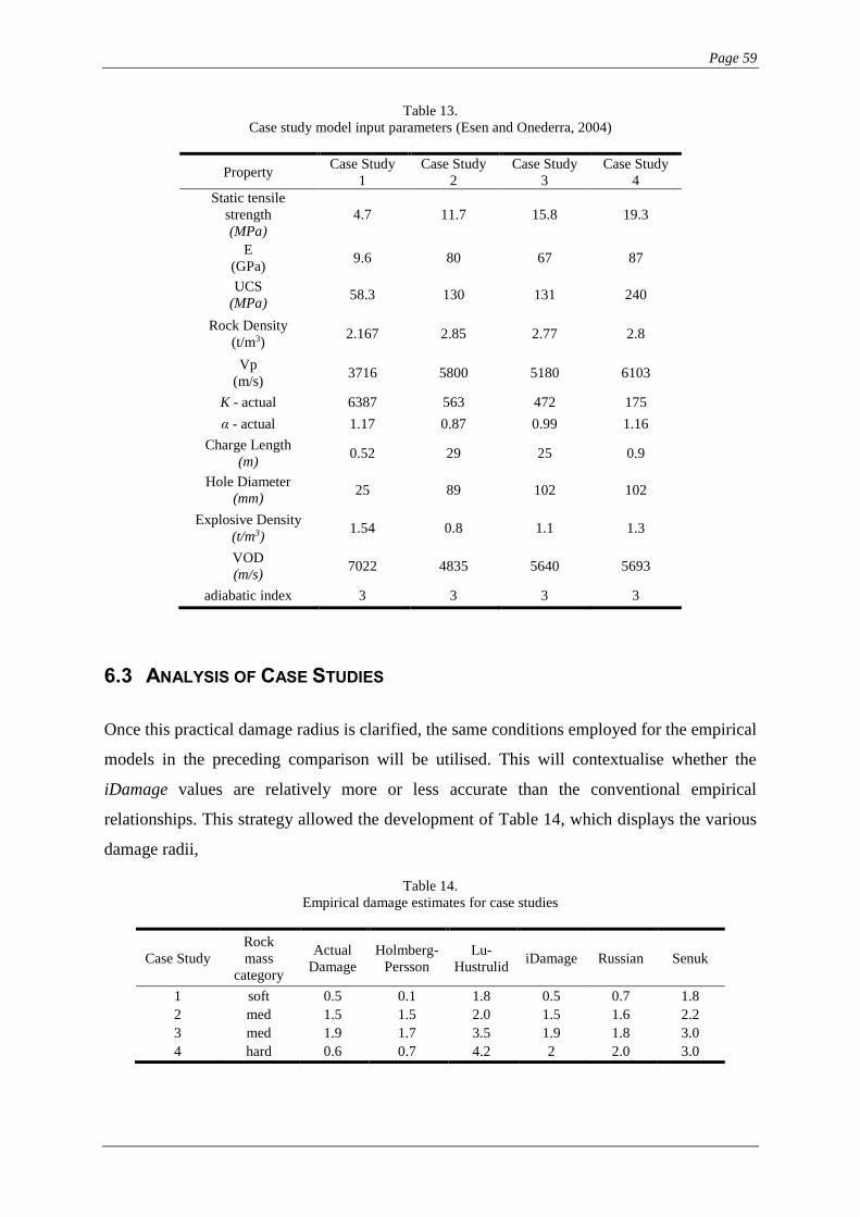
Page 59
Table 13.
Case study model input parameters (Esen and Onederra, 2004)
Property Case Study
1
Case Study
2
Case Study
3
Case Study
4
Static tensile
strength
(MPa)
4.7 11.7 15.8 19.3
E
(GPa) 9.6 80 67 87
UCS
(MPa) 58.3 130 131 240
Rock Density
(t/m3) 2.167 2.85 2.77 2.8
Vp
(m/s) 3716 5800 5180 6103
K - actual 6387 563 472 175
α - actual 1.17 0.87 0.99 1.16
Charge Length
(m) 0.52 29 25 0.9
Hole Diameter
(mm) 25 89 102 102
Explosive Density
(t/m3) 1.54 0.8 1.1 1.3
VOD
(m/s) 7022 4835 5640 5693
adiabatic index 3 3 3 3
6.3 ANALYSIS OF CASE STUDIES
Once this practical damage radius is clarified, the same conditions employed for the empirical
models in the preceding comparison will be utilised. This will contextualise whether the
iDamage values are relatively more or less accurate than the conventional empirical
relationships. This strategy allowed the development of Table 14, which displays the various
damage radii,
Table 14.
Empirical damage estimates for case studies
Case Study
Rock
mass
category
Actual
Damage
Holmberg-
Persson
Lu-
Hustrulid iDamage Russian Senuk
1 soft 0.5 0.1 1.8 0.5 0.7 1.8
2 med 1.5 1.5 2.0 1.5 1.6 2.2
3 med 1.9 1.7 3.5 1.9 1.8 3.0
4 hard 0.6 0.7 4.2 2 2.0 3.0
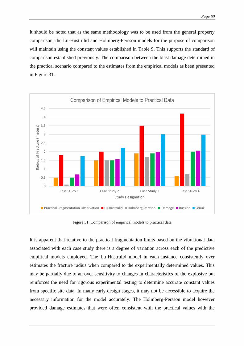
Page 60
It should be noted that as the same methodology was to be used from the general property
comparison, the Lu-Hustrulid and Holmberg-Persson models for the purpose of comparison
will maintain using the constant values established in Table 9. This supports the standard of
comparison established previously. The comparison between the blast damage determined in
the practical scenario compared to the estimates from the empirical models as been presented
in Figure 31.
Figure 31. Comparison of empirical models to practical data
It is apparent that relative to the practical fragmentation limits based on the vibrational data
associated with each case study there is a degree of variation across each of the predictive
empirical models employed. The Lu-Hustrulid model in each instance consistently over
estimates the fracture radius when compared to the experimentally determined values. This
may be partially due to an over sensitivity to changes in characteristics of the explosive but
reinforces the need for rigorous experimental testing to determine accurate constant values
from specific site data. In many early design stages, it may not be accessible to acquire the
necessary information for the model accurately. The Holmberg-Persson model however
provided damage estimates that were often consistent with the practical values with the
0
0.5
1
1.5
2
2.5
3
3.5
4
4.5
Case Study 1 Case Study 2 Case Study 3 Case Study 4
Rad
ius
of
Frac
ture
(m
eter
s)
Study Designation
Comparison of Empirical Models to Practical Data
Practical Fragmentation Observation Lu-Hustrulid Holmberg-Persson iDamage Russian Senuk
Page 61
exception of case study 1. From previous comparison observations, it can be proposed that the
varied explosive characteristics would not yield much impact on the output of the Holmberg-
Persson model. Similarly, the iDamage model conformed closely to the fracture radii
associated with the case studies though one anomaly remained; which in this instance was for
case study 4. The fourth case study featured a much lower true value for the attenuation
constant K. This may suggest that in applications where PPV analysis can determine a low K
value the iDamage model may give less than ideal results.
The Russian method is dependent on the cohesion and friction angle of the rock mass being
known. As this data was not known for the given rock masses in the case study data an
assumption was made to enable the comparison. Based on the UCS category of each rock mass
in the case study, an average cohesion used for the rock mass properties in the previous modular
comparison was applied. In most cases this allowed for a strong correlation with the iDamage
model where the Russian model demonstrated slightly higher (within 0.2m) fracture radii.
Concurrently the Russian model also over estimated the damage associated with the fourth case
study. The Senuk model consistently overestimated the extent of damage in all cases. This may
be a result of the rigidity of the stress concentration constant required for this model and an
over dependence on the tensile strength property of the rock mass. It consistently demonstrated
a poor fit to the practical situation.
6.4 CONCLUSION
The most consistent empirical models with the practical case data were the Holmberg-Persson
method and the iDamage method. Each demonstrating an anomaly in the consistency with the
practically determined damage ranges. The fault of the iDamage model in case study 4 may be
the result of the host rock mass having a low K stress attenuation constant. This describes a
state where the rock mass does not propagate stress waves as far; which may be the result of
uncategorised geological incongruities. The iDamage model has no true means of
incorporating this value but the Holmberg-Persson model does. This suggests that such
configurations of rock mass parameters and explosive conditions will yield a less accurate
predicted damage envelope from the iDamage model. This will need to be verified based on
further practical comparisons should further study be undertaken on this subject.
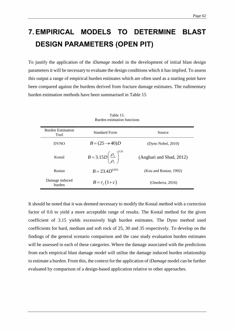
Page 62
7. EMPIRICAL MODELS TO DETERMINE BLAST
DESIGN PARAMETERS (OPEN PIT)
To justify the application of the iDamage model in the development of initial blast design
parameters it will be necessary to evaluate the design conditions which it has implied. To assess
this output a range of empirical burden estimates which are often used as a starting point have
been compared against the burdens derived from fracture damage estimates. The rudimentary
burden estimation methods have been summarised in Table 15
Table 15.
Burden estimation functions
Burden Estimation
Tool Standard Form Source
DYNO (25 40)B D (Dyno Nobel, 2010)
Kostal
0.33
3.15 e
r
B D
(Anghari and Shad, 2012)
Rustan 0.85523.4B D (Kou and Rustan, 1992)
Damage induced
burden 1fB r c (Onederra, 2016)
It should be noted that it was deemed necessary to modify the Kostal method with a correction
factor of 0.6 to yield a more acceptable range of results. The Kostal method for the given
coefficient of 3.15 yields excessively high burden estimates. The Dyno method used
coefficients for hard, medium and soft rock of 25, 30 and 35 respectively. To develop on the
findings of the general scenario comparison and the case study evaluation burden estimates
will be assessed in each of these categories. Where the damage associated with the predictions
from each empirical blast damage model will utilise the damage induced burden relationship
to estimate a burden. From this, the context for the application of iDamage model can be further
evaluated by comparison of a design-based application relative to other approaches.
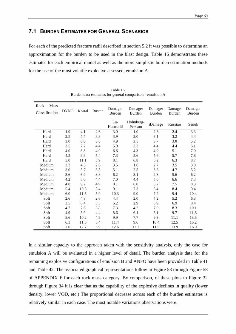
Page 63
7.1 BURDEN ESTIMATES FOR GENERAL SCENARIOS
For each of the predicted fracture radii described in section 5.2 it was possible to determine an
approximation for the burden to be used in the blast design. Table 16 demonstrates these
estimates for each empirical model as well as the more simplistic burden estimation methods
for the use of the most volatile explosive assessed, emulsion A.
Table 16.
Burden data estimates for general comparison - emulsion A
Rock Mass
Classification DYNO Kostal Rustan Damage:
Burden
Damage:
Burden
Damage:
Burden
Damage:
Burden
Damage:
Burden
Lu-
Hustrulid
Holmberg-
Persson iDamage Russian Senuk
Hard 1.9 4.1 2.6 3.0 1.0 2.3 2.4 3.3
Hard 2.5 5.5 3.3 3.9 2.0 3.1 3.2 4.4
Hard 3.0 6.6 3.8 4.9 2.5 3.7 3.8 5.2
Hard 3.5 7.7 4.4 5.9 3.3 4.4 4.4 6.1
Hard 4.0 8.8 4.9 6.6 4.3 4.9 5.1 7.0
Hard 4.5 9.9 5.4 7.3 5.6 5.6 5.7 7.8
Hard 5.0 11.1 5.9 8.1 6.8 6.2 6.3 8.7
Medium 2.3 4.3 2.6 3.5 1.6 2.7 3.5 3.9
Medium 3.0 5.7 3.3 5.1 2.5 3.6 4.7 5.2
Medium 3.6 6.9 3.8 6.2 3.1 4.3 5.6 6.2
Medium 4.2 8.0 4.4 7.0 4.4 5.0 6.6 7.3
Medium 4.8 9.2 4.9 8.1 6.0 5.7 7.5 8.3
Medium 5.4 10.3 5.4 9.1 7.3 6.4 8.4 9.4
Medium 6.0 11.5 5.9 10.3 9.0 7.2 9.4 10.4
Soft 2.6 4.8 2.6 4.4 2.0 4.2 5.2 6.3
Soft 3.5 6.4 3.3 6.2 2.9 5.9 6.9 8.4
Soft 4.2 7.6 3.8 7.3 4.2 7.0 8.3 10.1
Soft 4.9 8.9 4.4 8.6 6.1 8.1 9.7 11.8
Soft 5.6 10.2 4.9 9.9 7.7 9.3 11.1 13.5
Soft 6.3 11.5 5.4 11.4 9.6 10.4 12.5 15.2
Soft 7.0 12.7 5.9 12.6 12.2 11.5 13.9 16.9
In a similar capacity to the approach taken with the sensitivity analysis, only the case for
emulsion A will be evaluated in a higher level of detail. The burden analysis data for the
remaining explosive configurations of emulsion B and ANFO have been provided in Table 41
and Table 42. The associated graphical representations follow in Figure 53 through Figure 58
of APPENDIX F for each rock mass category. By comparison, of these plots to Figure 32
through Figure 34 it is clear that as the capability of the explosive declines in quality (lower
density, lower VOD, etc.) The proportional decrease across each of the burden estimates is
relatively similar in each case. The most notable variations observations were:
Page 64
burden estimates from the Lu-Hustrulid model fell at a disproportionally higher rate
than all other methods. This supports the observation prior that inferred an over
sensitivity to the change in explosive characteristics; and
the Kostal method conveys relatively larger over estimates for burden as the explosive
becomes less volatile.
In the remaining cases, typically the same trends observed in emulsion A have been replicated
in the alternate explosive compositions.
Figure 32. Burden estimates for emulsion A - hard rock
0.0
2.0
4.0
6.0
8.0
10.0
12.0
40 65 90 115 140 165 190 215
Esti
mat
ed B
urd
en (
met
ers)
Borehole Diameter
Burden Empirical Estimation Comparison - Emulsion A: Hard Rock
DYNO
Kostal
Rustan
Damage Burden: Lu-Hustrulid
Damage Burden: Holmberg-Persson
Damage Burden: iDamage
Damage Burden: Russian
Damage Burden: Senuk
Page 65
Figure 33. Burden estimates for emulsion A - medium rock
Figure 34. Burden estimates for emulsion A - soft rock
0.0
2.0
4.0
6.0
8.0
10.0
12.0
14.0
40 65 90 115 140 165 190 215
Esti
mat
ed B
urd
en (
met
ers)
Borehole Diameter
Burden Empirical Estimation Comparison - Emulsion A: Medium Rock
DYNO
Kostal
Rustan
Damage Burden: Lu-Hustrulid
Damage Burden: Holmberg-Persson
Damage Burden: iDamage
Damage Burden: Russian
Damage Burden: Senuk
0.0
2.0
4.0
6.0
8.0
10.0
12.0
14.0
16.0
18.0
40 65 90 115 140 165 190 215
Esti
mat
ed B
urd
en (
met
ers)
Borehole Diameter
Burden Empirical Estimation Comparison - Emulsion A: Soft Rock
DYNO
Kostal
Rustan
Damage Burden: Lu-Hustrulid
Damage Burden: Holmberg-Persson
Damage Burden: iDamage
Damage Burden: Russian
Damage Burden: Senuk
Page 66
As the rock mass quality falls from Figure 32 to Figure 34 both the Dyno and Rustan methods
do not change as they have no means of considering change in the rock mass or explosive
properties. Hence in medium to softer rock these methods could infer the need for an
excessively small blasting pattern which may result in overbreak or air blast issues (Zhang,
2016). The modified Kostal model over estimates the capability of the explosive to induce
damage in hard and medium rock qualities evidenced by the large disparity in these values. In
soft rock however, it aligns closely to the Lu-Hustrulid and Russian models. The behaviour of
the burden estimates from the empirical blast damage models closely aligns with that in the
fracture radii determination. For instance the burden estimates of Lu-Hustrulid, Russian and
Senuk models are relatively higher for emulsion A. The Holmberg-Persson model yields a
much tighter burden than most models until a higher borehole diameter is utilised. From this
analysis, it is apparent that the iDamage model continues to offer a more continuous burden
prediction that is central to most other estimates. The iDamage model is not prone to the over
estimation of the Russian, Senuk or Kostal models but still manages to consider the changes in
the rock mass conditions where the Dyno and Rustan models do not. In terms of burden
estimation, the iDamage model would seem to be the least prone to an inappropriately drastic
change relative to the variation of the input parameters.
7.2 BURDEN AND SPACING ESTIMATES FOR CASE STUDY DATA
Burden estimates can be combined with pre-established rules of thumb, that continue to
dominate blast design guidelines in industry today, to estimate other parameters such as
spacing, height, sub-grade, stemming and more (Dyno Nobel, 2010) To confirm the findings
in the burden analysis for the general scenario the case studies will be similarly investigated.
These calculated burdens will be used to define a spacing, which may generate a rudimentary
blasting pattern. Table 17 andTable 17Table 18 detail the burden and spacing for the case
studies
Page 67
Table 17.
Burden estimation data for case studies
Case
Study DYNO Kostal Rustan
Damage:
Burden
Damage:
Burden
Damage:
Burden
Damage:
Burden
Damage:
Burden Damage: Burden
(m)
(m)
(m)
Lu-
Hustrulid
(m)
Holmberg-
Persson
(m)
iDamage
(m)
Russian
(m)
Senuk
(m)
Practical
Damage Range
(m)
1 0.6 1.7 1.0 2.3 0.1 0.7 0.9 2.3 0.7
2 2.2 4.4 3.0 2.6 2.0 2.0 2.0 2.9 2.0
3 2.6 5.6 3.3 4.6 2.2 2.5 2.6 3.9 2.5
4 2.6 5.9 3.3 5.5 0.9 2.6 2.7 3.9 0.8
Table 18.
Spacing estimation data for case studies
Case
Study DYNO Kostal Rustan
Damage:
Burden
Damage:
Burden
Damage:
Burden
Damage:
Burden
Damage:
Burden
Damage:
Burden
(m)
(m)
(m)
Lu-
Hustrulid
(m)
Holmberg-
Persson
(m)
iDamage
(m)
Russian
(m)
Senuk
(m)
Practical
Damage
Range
(m)
1 0.8 2.1 1.2 2.9 0.2 0.8 1.1 2.8 0.8
2 2.8 5.4 3.7 3.3 2.4 2.4 2.6 3.6 2.4
3 3.2 7.0 4.2 5.7 2.8 3.1 3.2 4.9 3.1
4 3.2 7.4 4.2 6.8 1.1 3.3 3.4 4.8 1.0
The spacing is determined by a standard correlation that states the spacing bust be between
12 times the burden distance. Commonly a nominal value of 1.25 is used (Dyno Nobel, 2010)
and this standard was utilised in the determination of the spacing for the rock mass explosive
configurations outlined in the case study data from Esen and Onederra (2004). .A graphical
representation of the burden and spacing for each method was developed in Figure 35 and
Figure 36 such that it could be compared to the burden and spacing derived for the practically
established damage in the case studies.
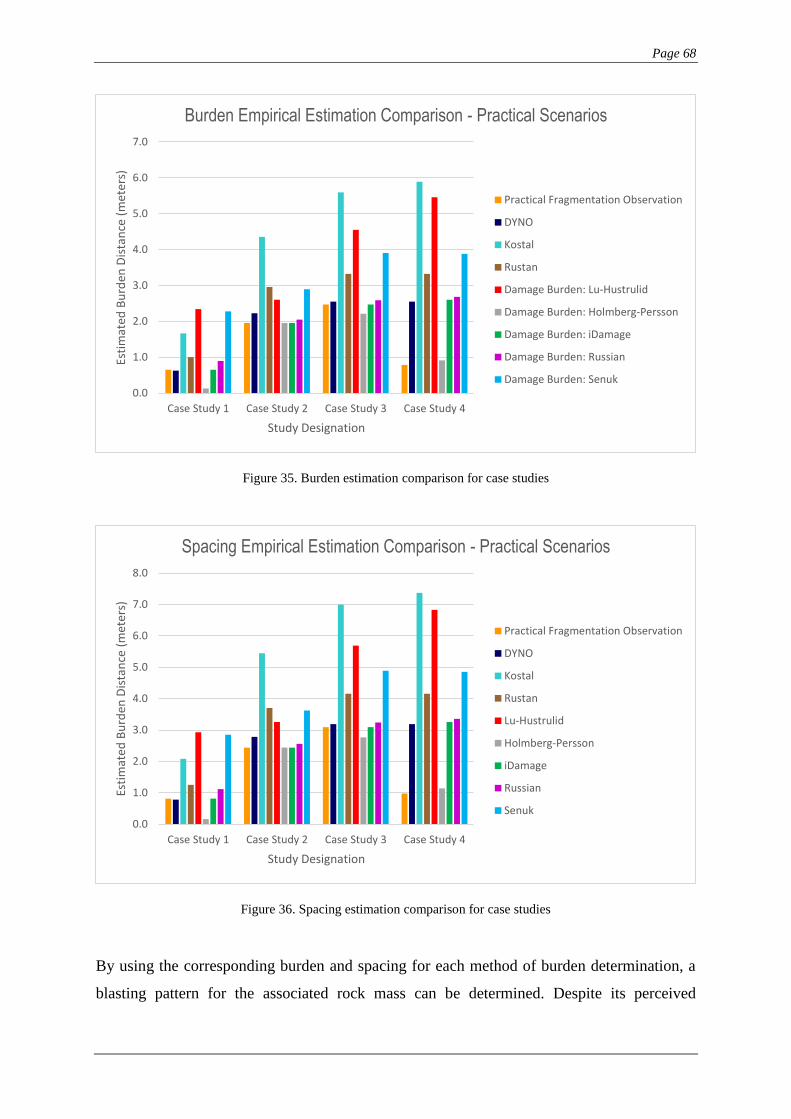
Page 68
Figure 35. Burden estimation comparison for case studies
Figure 36. Spacing estimation comparison for case studies
By using the corresponding burden and spacing for each method of burden determination, a
blasting pattern for the associated rock mass can be determined. Despite its perceived
0.0
1.0
2.0
3.0
4.0
5.0
6.0
7.0
Case Study 1 Case Study 2 Case Study 3 Case Study 4
Esti
mat
ed B
urd
en D
ista
nce
(m
eter
s)
Study Designation
Burden Empirical Estimation Comparison - Practical Scenarios
Practical Fragmentation Observation
DYNO
Kostal
Rustan
Damage Burden: Lu-Hustrulid
Damage Burden: Holmberg-Persson
Damage Burden: iDamage
Damage Burden: Russian
Damage Burden: Senuk
0.0
1.0
2.0
3.0
4.0
5.0
6.0
7.0
8.0
Case Study 1 Case Study 2 Case Study 3 Case Study 4
Esti
mat
ed B
urd
en D
ista
nce
(m
eter
s)
Study Designation
Spacing Empirical Estimation Comparison - Practical Scenarios
Practical Fragmentation Observation
DYNO
Kostal
Rustan
Lu-Hustrulid
Holmberg-Persson
iDamage
Russian
Senuk
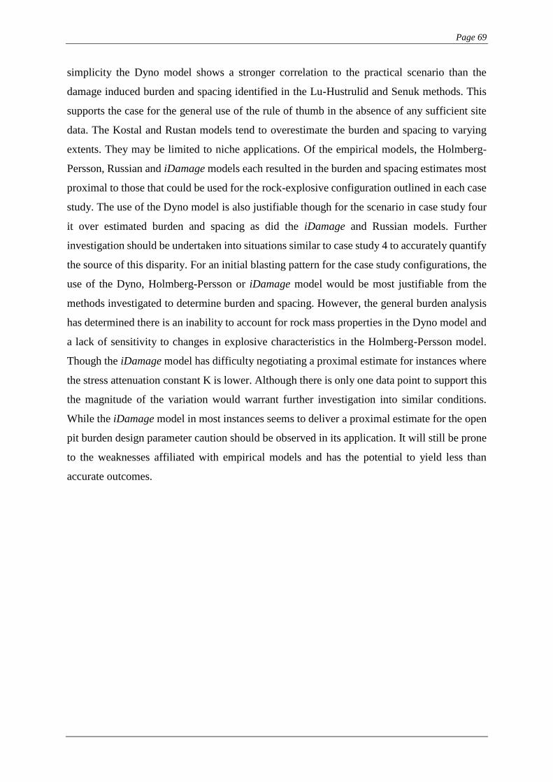
Page 69
simplicity the Dyno model shows a stronger correlation to the practical scenario than the
damage induced burden and spacing identified in the Lu-Hustrulid and Senuk methods. This
supports the case for the general use of the rule of thumb in the absence of any sufficient site
data. The Kostal and Rustan models tend to overestimate the burden and spacing to varying
extents. They may be limited to niche applications. Of the empirical models, the Holmberg-
Persson, Russian and iDamage models each resulted in the burden and spacing estimates most
proximal to those that could be used for the rock-explosive configuration outlined in each case
study. The use of the Dyno model is also justifiable though for the scenario in case study four
it over estimated burden and spacing as did the iDamage and Russian models. Further
investigation should be undertaken into situations similar to case study 4 to accurately quantify
the source of this disparity. For an initial blasting pattern for the case study configurations, the
use of the Dyno, Holmberg-Persson or iDamage model would be most justifiable from the
methods investigated to determine burden and spacing. However, the general burden analysis
has determined there is an inability to account for rock mass properties in the Dyno model and
a lack of sensitivity to changes in explosive characteristics in the Holmberg-Persson model.
Though the iDamage model has difficulty negotiating a proximal estimate for instances where
the stress attenuation constant K is lower. Although there is only one data point to support this
the magnitude of the variation would warrant further investigation into similar conditions.
While the iDamage model in most instances seems to deliver a proximal estimate for the open
pit burden design parameter caution should be observed in its application. It will still be prone
to the weaknesses affiliated with empirical models and has the potential to yield less than
accurate outcomes.
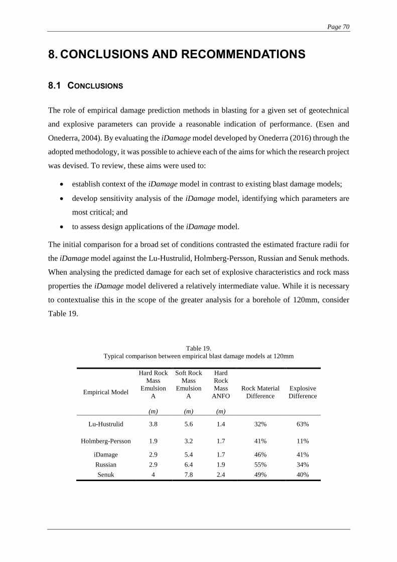
Page 70
8. CONCLUSIONS AND RECOMMENDATIONS
8.1 CONCLUSIONS
The role of empirical damage prediction methods in blasting for a given set of geotechnical
and explosive parameters can provide a reasonable indication of performance. (Esen and
Onederra, 2004). By evaluating the iDamage model developed by Onederra (2016) through the
adopted methodology, it was possible to achieve each of the aims for which the research project
was devised. To review, these aims were used to:
establish context of the iDamage model in contrast to existing blast damage models;
develop sensitivity analysis of the iDamage model, identifying which parameters are
most critical; and
to assess design applications of the iDamage model.
The initial comparison for a broad set of conditions contrasted the estimated fracture radii for
the iDamage model against the Lu-Hustrulid, Holmberg-Persson, Russian and Senuk methods.
When analysing the predicted damage for each set of explosive characteristics and rock mass
properties the iDamage model delivered a relatively intermediate value. While it is necessary
to contextualise this in the scope of the greater analysis for a borehole of 120mm, consider
Table 19.
Table 19.
Typical comparison between empirical blast damage models at 120mm
Empirical Model
Hard Rock
Mass
Emulsion
A
(m)
Soft Rock
Mass
Emulsion
A
(m)
Hard
Rock
Mass
ANFO
(m)
Rock Material
Difference
Explosive
Difference
Lu-Hustrulid 3.8 5.6 1.4 32% 63%
Holmberg-Persson 1.9 3.2 1.7 41% 11%
iDamage 2.9 5.4 1.7 46% 41%
Russian 2.9 6.4 1.9 55% 34%
Senuk 4 7.8 2.4 49% 40%
Page 71
The general tendency established for the data points at the 120mm scenario was generally
reflected across all trials analysed with few notable anomalies identified in the broader analysis.
Essentially the iDamage model reflected the change in rock mass more so than the Lu-
Hustrulid and Holmberg-Persson methods but less so than the Russian and Senuk models. Also
as hypothesised, based on the descriptions of the empirical models, the iDamage model
reflected a larger variation in damage for a controlled change in explosive than the Holmberg-
Persson, Russian and Senuk models, but less so than the Lu-Hustrulid model. This substantiates
the use of the iDamage model as a tool of blast design as it appropriates the changes in the rock
mass and the explosive in a more stable capacity to yield a more central estimate of fracture
radii relative to other blast damage models.
The sensitivity analysis was undertaken in a deterministic capacity to establish which
parameters effected the greatest influence over the iDamage model. While this does not
account for the presence of interaction between rock mass properties, it is beneficial to know
which parameters to prioritise when using the iDamage predictions. A priority order for the
sensitivity of parameters was established. It was determined for emulsion A and B that the
model was most sensitive to a range of parameters that described both the rock mass and the
explosive i.e. charge diameter, static tensile strength, VOD and p-wave velocity. While for the
lower yield explosive (ANFO), the explosive properties dominated i.e. Charge diameter, VOD
and explosive density. Being aware of these sensitivities will help to optimise the application
of the iDamage model, although at higher levels of study the interactions between parameters
and some of the discrepancies of deterministic methodology must be addressed.
The damage prediction empirical methods utilised in the comparison were applied to a range
of practical scenarios in a collection of case studies composed by Esen and Onederra (2004)
from which an accurate value for blast damage was already established. In each case the Senuk
and Lu-Hustrulid models consistently overestimated breakage. The Russian model yielded
slightly higher (within 0.2m) values than the iDamage model. While the iDamage model and
Holmberg-Persson model correlated most proximally to the practical fragmentation radius
determined. Although the iDamage model largely over estimated damage in the only instance
where the stress attenuation constant of K was far lower than the other trials. Once more, this
analysis generally supported the use of the iDamage model.
Page 72
The final component of the evaluation was to apply the determined fracture radii for the
empirical models in the general comparison and in the case studies to obtain estimates for
burden. Coupled with other rules of thumb that are regularly used in early stages of blast design
the burden values determined can provide the means to numerous parameters including, but
not limited to, spacing, stemming and subgrade (Dyno Nobel, 2010). The means to determine
burden analysed included more simple rules of thumb (Dyno formula, Rustan formula and
Kostal formula) as well as the damage induced burden formula. The Dyno and Rustan models
could not account for changes in any other parameter beyond diameter, which may give a
distinct advantage to the remaining burden estimation tools that do. In its present form however
the Kostal formula required a correction factor which still resulted in overestimation; albeit
dampened in magnitude. The burden determined from damage models, as expected, accounted
for changes in the explosive and geotechnical parameters in proportion to the respective model.
Hence the burden identified in the iDamage model gave a centrally based estimate. When
burden as well as spacing projections were determined for the case study data the most
proximal design criteria estimates were based on the: Dyno, iDamage and Holmberg-Persson
models.
The iDamage model has demonstrated relative centrality of damage estimates and a balanced
sensitivity to a range of parameters describing both explosive, as well as geotechnical
properties of the blasting condition. Concurrently, the iDamage model has been evaluated and
found to be an effective tool to supplement the initial phases of blast design; at least within the
scope of this study.
Page 73
8.2 RECOMMENDATIONS
While this research project has provided a reasonable evaluation of the iDamage blast model,
there are still numerous capacities in which this study can be further enhanced. Through the
expansion of the explosive and geotechnical data sets on which the general comparison was
based, any conclusions may be further supported by having a wider sample upon which to base
conclusions. A comparison to more varied empirical models would also help to confirm the
context for the projected damage associated with the iDamage model. Specifically those that
quantify properties not specified explicitly by the iDamage model. For instance, the McHugh
model is predicated on the assumption gas expansion is the dominant rock breakage mechanism
(McHugh, 1983).
The sensitivity analysis may be improved from its current deterministic basis. While this served
the needs of this evaluation at a base level it does not effectively account for uncertainty in the
input parameters, neither does it consider the level of interaction and co-dependence between
rock mass parameters. It should be recognised that this might change the relative sensitivities
of these parameters. Hence, it would be ideal to actively pursue a sensitivity analysis that
utilised at least a first order approach to model the behaviour of the input parameters. Second
order sensitivity may supplement this but it is suffice to state a first order analysis should be
undertaken initially. By upgrading the sensitivity analysis to be supported by stochastic
methodology, the understanding of the internal relationships for the iDamage model would be
improved and by extension, the applications to practical scenarios would be benefited.
This evaluation’s comparison to four case studies was still somewhat limited. It would be ideal
to develop a more substantial range of practical blasting experiments to which the estimates of
the iDamage model could be appropriately compared. This may identify any situations in
which the iDamage model is less or more effective in its use and may establish an envelope for
ideal application. Although, empirical models alone cannot define the extent of blast
performance to a level of accuracy required by some sectors of industry. The characteristics
identified as acceptable in the empirical model are those that will warrant further investigation.
The higher detail modelling techniques include numerical/mechanistic modelling, HSBM and
MBM. (Read and Stacey, 2009) Using such methods for verification would also be a beneficial
supplement to this analysis
Page 74
For further work it would be worthwhile to run a blast design based on the iDamage model that
is being run in tandem with a design developed using industry standards. This would integrate
the iDamage model into the process for a practical blast design. Comparisons could then be
made against the common industry standard that is pursued and the design parameters
developed from the model investigated by this research project. This would contextualise the
downstream impacts associated with using the iDamage model may have on practical
applications to industry.
In summation, if these recommendations were undertaken it is anticipated that the evaluation
of the model would yield more justifiable conclusions. This would substantiate the identified
appropriateness of the induction of the iDamage empirical blast damage model into the blast
design process
Page 75
9. REFERENCES
Alvares, R, A, Gomes, R, C, and Innocentini, M, D, M, 2004. in Landslides: evaluation and
stabilization (ed;W, A, Lacerda, M, Ehrlich, S, A, B, Fontoura and A, S, F, Sayao)
pp527-532 (A.A. Balkema: London)
An, X, M, and Ma, G, W, 2008. Numerical simulation of blasting induced fractures,
International journal of rock mechanics and mining sciences, 45 (8):966-975
Ahangari, K, and Shad, H, 2012. An empirical relation to calculate the proper burden in blast
design, International journal of rock mechanics and mining sciences, 56 (8):121-126
Attewell, P, B, and Farmer, I, W, 1976. Principles of engineering geology, pp182-201
(Dordrecht Springer: Amsterdam)
Bawden, W, F, Katsabanis, P, D, and Yang, R, 1996. A New Constitutive Model for Blast,
International Journal for Rock Mechanics, 33(3):245-254
BHP, 2009. Risk matrix and impacts table [online].Available from <http://www.bhpbilliton.
com/~/media/bhp/documents/> [Accessed: 18 May 2016]
Brady, B, H, G, and Brown, E, T, 2004. Rock mechanics: for underground mining, pp518-
542 (Kluwer Academic Publishers: Boston)
Cai, M, 2010. Practical estimates of tensile strength and Hoek-Brown strength parameter mi
of brittle rocks, Rock Mechanics and Rock Engineering, 43(2):167-184
Page 76
Cho, S, H, Kaneko, K, and Ogata, Y, 2003. Strain-rate dependency of the dynamic tensile
strength of rock, International Journal of Rock Mechanics and Mining Sciences,
40(5):763-777
Comparerocks (CR), 2015. Properties of rocks [online]. Available from < http://www.compa
rerocks.com/en > [Accessed: 13 September 2016]
Crowther, G, Lizotte, Y, Scoble, M, and Singh, A, 1991. Characterization of underground
rock fragmentation, Geotechnical and Geological Engineering, 9(5):93-107.
Daehnke, A., Knasmillner, R.E. and Rossmanith, H.P., 1996. Blast-induced dynamic fracture
propagation in Rock Fragmentation by Blasting (ed: B. Mohanty), pp 13-18 (A.A.
Bakelma: Rotterdam)
Diederichs, M, S, and Perras, M, A, 2013. A review of tensile strength of rock: concepts and
testing, Geotechnical and Geological Engineering, 32(2):525-546
Dijkman, J, P, M, Stedinger, J, R, and Villars, M, T, 2005. Resources Systems and
Management, Model Sensitivity and Uncertainty Analysis pp261-273 (UNESCO: Paris)
Dhawan, K, R, and Muralidhar, B, 2015. Relationship between static and two types of
dynamic moduli for different rocks, Indian Geotechnical Journal, 45(3):341-348
Duan, K, Kwok, F,C,Y, and Tham, L G, 2013. The behaviour of brittle rocks in Rock
characterisation, modelling and engineering design methods. (ed: X, Feng), pp 23-31
(CRC Press: London)
Dyno Nobel, 2010. Blasting and explosives: quick reference guide [online]. Available from
<https://www.leg.state.mn.us/docs/2015...> [Accessed: 29 September 2016]
Page 77
Esen, S, and Onederra, I, 2004. An alternative approach to determine the Holmberg-Persson
constants for modelling near field peak particle velocity attenuation, Fragblast,
2(3):61-84
Erickson, K,B 2014. Investigating the extent of damage from a single blasthole, Masters
Thesis (Published), Chapter 2, pp 6-31 University of Utah, Salt Lake City,
Evangelista, A, and Picarelli, L, 1998. The geotechnics of hard soils - soft rocks,1191p (A.
A. Balkema: Rotterdam)
Hu, S and Yu, F, R, 2014. Calculation of both high velocity detonation and low velocity
detonation processes using a unified model [online]. Available from < http://www.csit.
carleton.ca/ > [Accessed: 13 September 2016]
Keceli, A, 2012. Soil parameters which can be determined using seismic velocities, Jeofiznik,
8(130):17-29
Kostić, S, Perc, M, Trajković, S, and Vasović, N, 2013. Predictions of experimentally
observed stochastic ground vibrations induced by blasting [online], PLoS One, 8.
Available from: < journals.plos.org/plosone… > [Accessed 18 April 2016].
Kou, S,Q, and Rustan, A 1992. Burden related to blasthole diameter in rock blasting,
International Journal of Rock Mechanics and Mining Sciences, 29(6):543-553
Li, Q, M, Lu, Y, B, and Ma, G, W, 2010. Numerical investigation of the dynamic
compressive strength of rocks based on split Hopkinson pressure bar tests,
International Journal of Rock Mechanics and Mining Sciences, 47(5):829-838
Page 78
Look, B, G, 2014. Handbook of geotechnical investigation and design tables, pp113-123
(CRC Press: London)
Mahadevan, E, G, 2013. Ammonium nitrate explosives for civil applications: slurries,
emulsions and ammonium nitrate fuel oils, pp31-53 (Wiley-VCH: Weinheim)
Mavko, G, 2014. Conceptual overview of rock and fluid factors that impact seismic velocity
and impedance [online]. Available from < https://pangea.stanford.edu/courses/gp262/
Notes /8.SeismicVelocity.pdf > [Accessed: 13 September 2016]
McHugh, S. 1983. Crack extension caused by internal gas pressure compared with extension
caused by tensile stress. International journal of fracture, 21(3):163–176.
Mosinets, V. N., 1966. Mechanisms of rock breaking by blasting in relation to its fracturing
and elastic constants, Soviet Mining Science, 2, 492-499
Narendrula, R, and Singh, S, P, 2004. Assessment and prediction of rock mass damage by
blast vibrations in Mine Planning and Equipment Selection 2004 (ed: M. Hardygóra, G.
Paszkowska and M. Sikora.), pp 317-322 (A.A. Bakelma: Rotterdam)
Ndibalema, A, 2008. Capturing economic benefits from blasting. The Southern African
Institute of Mining and Metallurgy [online]. Available from <http://www.saimm.co.za>
[Accessed: 17 May 2016]
Onederra, I, 2016. Empirical Estimates of the fracturing zone around a fully coupled
explosive charge, (unpublished), University of Queensland, Brisbane.
Onederra, I, 2016. Personal communication (Research Project Supervisor): University of
Queensland, 23 September 2016.
Page 79
Palmström, A, 1995. Methods to quantify the parameters applied in the RMi, PhD
Dissertation (Published), Oslo University, Oslo.
Palmström, A, and Singh, R, 2001. The deformation modulus of rock masses - comparisons
between insitu tests and indirect estimates. Tunnelling and Underground Space
Technology, 16(3):115-131
Read, J, and Stacey, P, 2009. Guidelines for open pit slope design, pp294-310 (CSIRO
Publishing: Collingwood)
Rinne, M, Shen, B, and Siren, T, 2014. Modelling fracture propagation in anisotropic rock
mass, Rock mechanics and rock engineering, 48(14):1067-1081
Schön, J, 2011. Physical properties of rocks: a workbook, pp245-271 (Elsevier: Oxford)
Schultz, R, A, 1994. Comparative rock mass strengths of basalt and tuff and some
planetological implications, in Proceedings lunar planetary science conference, Texas
USA 1217p, (Rock fracture group: Reno)
Sharma, P, K, and Singh, T, N, 2008. A correlation between p-wave velocity, impact strength
index, slake durability index and uniaxial compressive strength, Bulletin of Engineering
Geology and the Environment, 67(1):17-22
Sharma, P, D, 2012. Rock breakage and blast design considerations in open pit
[online].Available from <https://miningandblasting.wordpress.com/> [Accessed: 17
May 2016]
Page 80
Singh, S.P., 2001. The influence of geology on blast damage. Ontario CIM Bulletin, Vol.
94(1048):121-127
Sun, C, 2013. Damage zone prediction for rock blasting, PhD dissertation (published)
University of Utah, Salt Lake City. Chapter 2, 14-41 p.
Unlu, T, and Yilmaz, O, 2014. An application of the modified holmberg-persson approach for
tunnel blasting design, Tunnelling and underground space technology, 43(8):113-122
Zhang, Z, 2016. Rock fracture and blasting, theory and applications pp 197-270 (Elsevier:
Oxford)
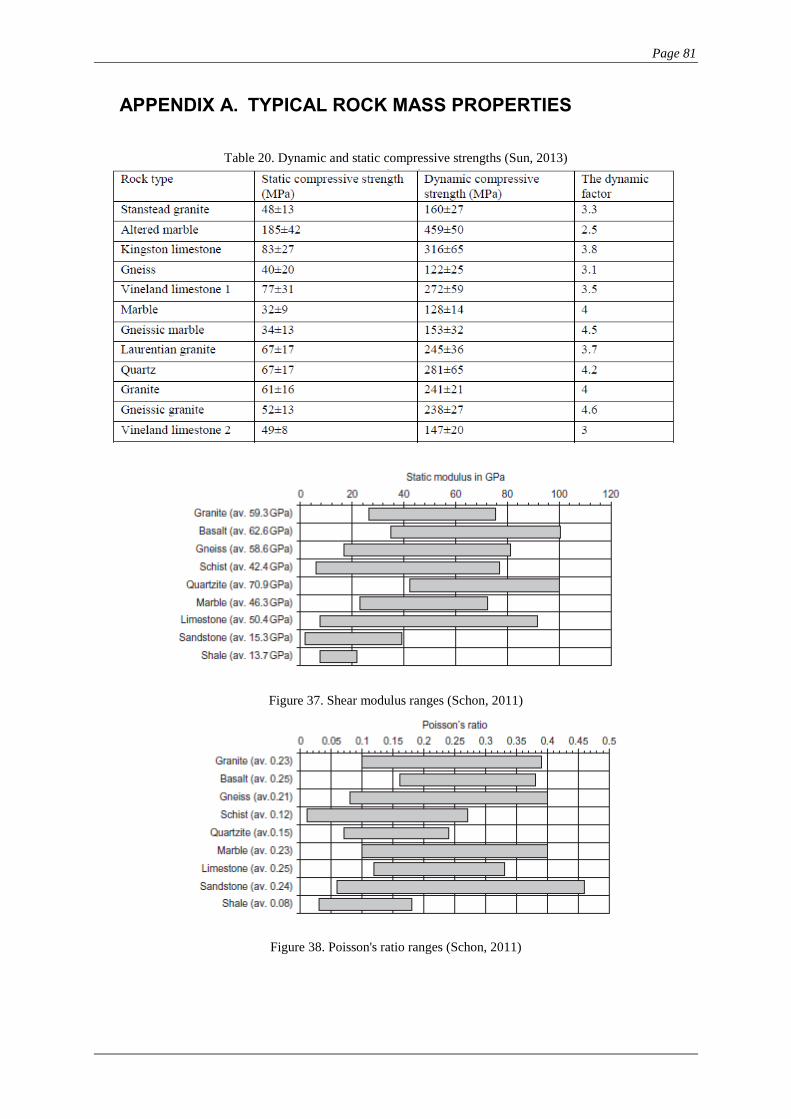
Page 81
APPENDIX A. TYPICAL ROCK MASS PROPERTIES
Table 20. Dynamic and static compressive strengths (Sun, 2013)
Figure 37. Shear modulus ranges (Schon, 2011)
Figure 38. Poisson's ratio ranges (Schon, 2011)
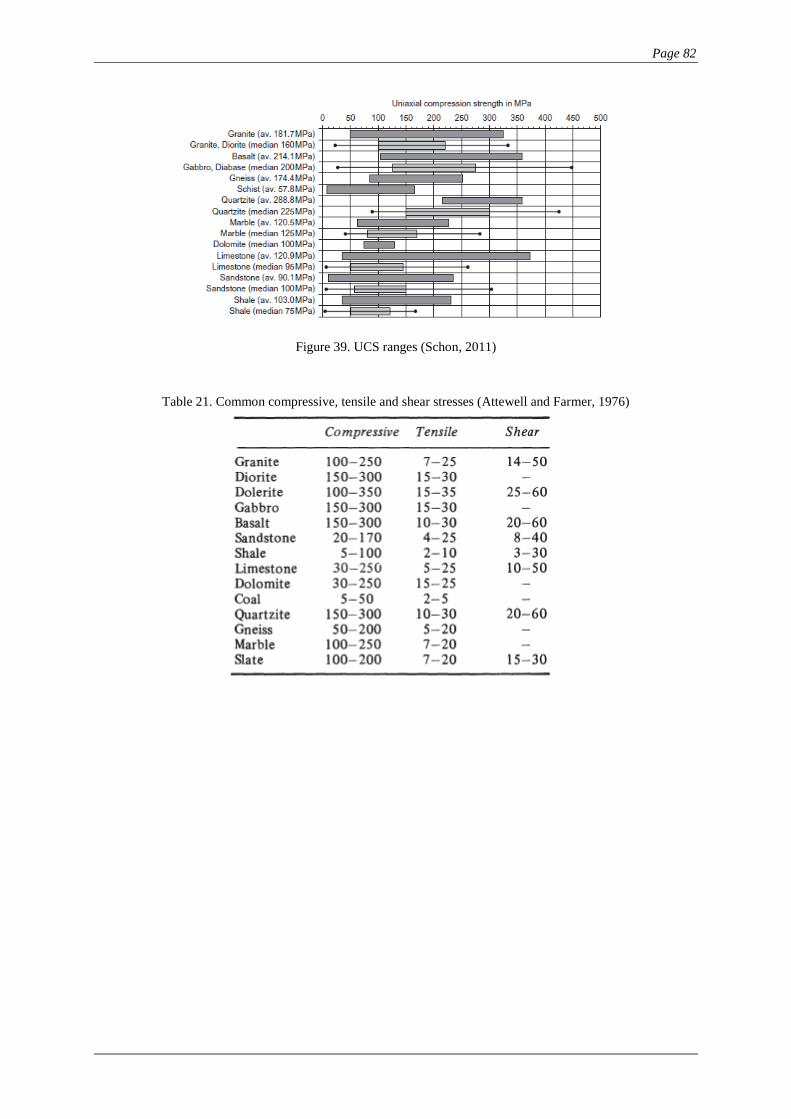
Page 82
Figure 39. UCS ranges (Schon, 2011)
Table 21. Common compressive, tensile and shear stresses (Attewell and Farmer, 1976)
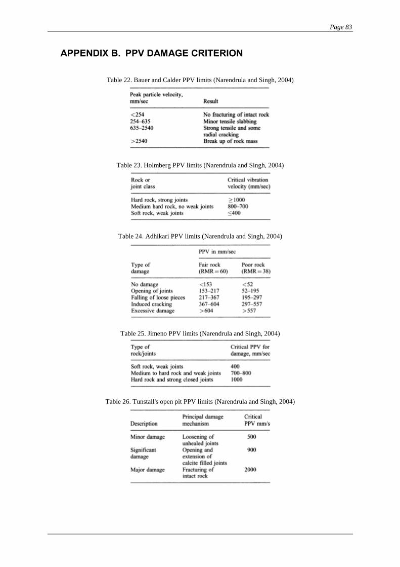
Page 83
APPENDIX B. PPV DAMAGE CRITERION
Table 22. Bauer and Calder PPV limits (Narendrula and Singh, 2004)
Table 23. Holmberg PPV limits (Narendrula and Singh, 2004)
Table 24. Adhikari PPV limits (Narendrula and Singh, 2004)
Table 25. Jimeno PPV limits (Narendrula and Singh, 2004)
Table 26. Tunstall's open pit PPV limits (Narendrula and Singh, 2004)
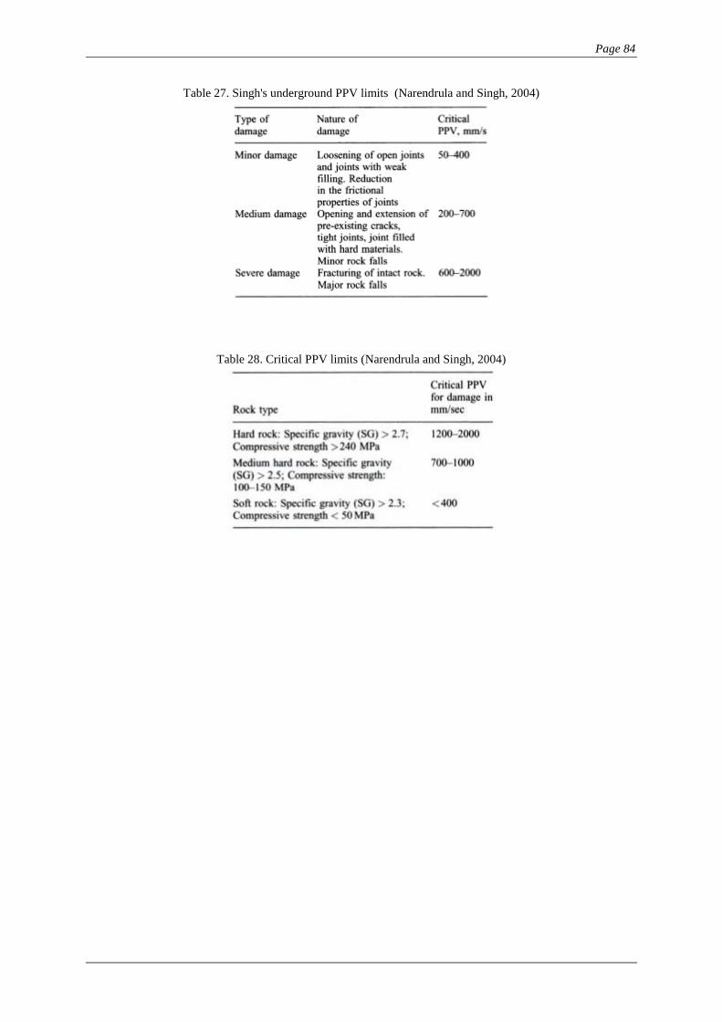
Page 84
Table 27. Singh's underground PPV limits (Narendrula and Singh, 2004)
Table 28. Critical PPV limits (Narendrula and Singh, 2004)
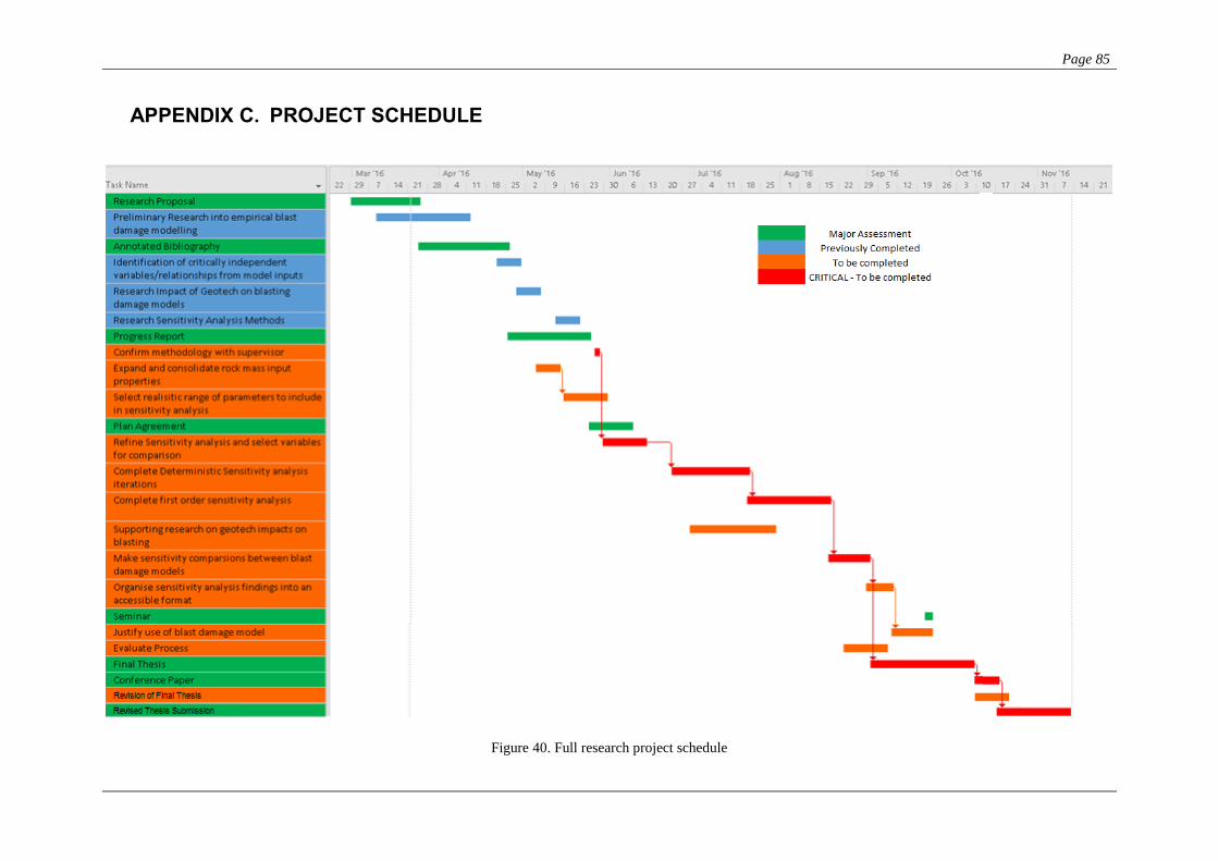
Page 85
APPENDIX C. PROJECT SCHEDULE
Figure 40. Full research project schedule
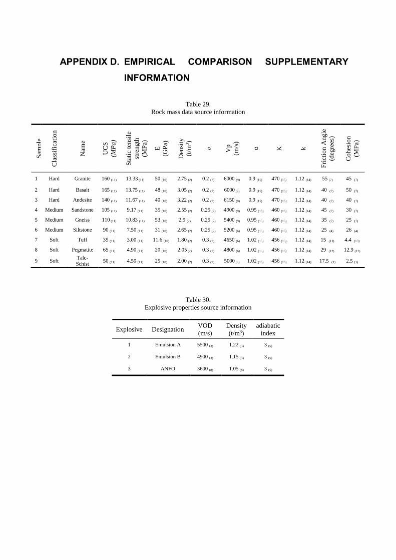
APPENDIX D. EMPIRICAL COMPARISON SUPPLEMENTARY
INFORMATION
Table 29.
Rock mass data source information
Table 30.
Explosive properties source information
Explosive Designation VOD
(m/s)
Density
(t/m3)
adiabatic
index
1 Emulsion A 5500 (3) 1.22 (3) 3 (5)
2 Emulsion B 4900 (3) 1.15 (3) 3 (5)
3 ANFO 3600 (8) 1.05 (8) 3 (5)
Sam
ple
Cla
ssif
icat
ion
Nam
e
UC
S
(MP
a)
Sta
tic
ten
sile
stre
ng
th
(MP
a)
E
(GP
a)
Den
sity
(t/m
3)
υ
Vp
(m/s
)
α
K
k
Fri
ctio
n A
ng
le
(deg
rees
)
Co
hes
ion
(MP
a)
1 Hard Granite 160 (11) 13.33 (11) 50 (10) 2.75 (2) 0.2 (7) 6000 (9) 0.9 (15) 470 (15) 1.12 (14) 55 (7) 45 (7)
2 Hard Basalt 165 (11) 13.75 (11) 48 (10) 3.05 (2) 0.2 (7) 6000 (9) 0.9 (15) 470 (15) 1.12 (14) 40 (7) 50 (7)
3 Hard Andesite 140 (11) 11.67 (11) 40 (10) 3.22 (2) 0.2 (7) 6150 (9) 0.9 (15) 470 (15) 1.12 (14) 40 (7) 40 (7)
4 Medium Sandstone 105 (11) 9.17 (11) 35 (10) 2.55 (2) 0.25 (7) 4900 (9) 0.95 (15) 460 (15) 1.12 (14) 45 (7) 30 (7)
5 Medium Gneiss 110 (11) 10.83 (11) 53 (10) 2.9 (2) 0.25 (7) 5400 (9) 0.95 (15) 460 (15) 1.12 (14) 35 (7) 25 (7)
6 Medium Siltstone 90 (11) 7.50 (11) 31 (10) 2.65 (2) 0.25 (7) 5200 (6) 0.95 (15) 460 (15) 1.12 (14) 25 (4) 26 (4)
7 Soft Tuff 35 (11) 3.00 (11) 11.6 (10) 1.80 (2) 0.3 (7) 4650 (6) 1.02 (15) 456 (15) 1.12 (14) 15 (13) 4.4 (13)
8 Soft Pegmatite 65 (11) 4.90 (11) 20 (10) 2.05 (2) 0.3 (7) 4800 (6) 1.02 (15) 456 (15) 1.12 (14) 29 (12) 12.9 (12)
9 Soft Talc-
Schist 50 (11) 4.50 (11) 25 (10) 2.00 (2) 0.3 (7) 5000 (6) 1.02 (15) 456 (15) 1.12 (14) 17.5 (1) 2.5 (1)
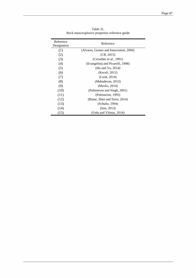
Page 87
Table 31.
Rock mass/explosive properties reference guide
Reference
Designation Reference
(1) (Alvares, Gomes and Innocentini, 2004)
(2) (CR, 2015)
(3) (Crowther et al., 1991)
(4) (Evangelista and Picarelli, 1998)
(5) (Hu and Yu, 2014)
(6) (Keceli, 2012)
(7) (Look, 2014)
(8) (Mahadevan, 2013)
(9) (Mavko, 2014)
(10) (Palmstrom and Singh, 2001)
(11) (Palmstrom, 1995)
(12) (Rinne, Shen and Siren, 2014)
(13) (Schultz, 1994)
(14) (Sun, 2013)
(15) (Unlu and Yilmaz, 2014)
Page 88
Table 32.
Empirical blast damage estimates using Emulsion A
Granite Basalt Andesite Sandstone Gneiss Siltstone Tuff Pegmatite Talc-
Schist
Empirical Model Borehole
Diameter
Damage
Range
(m)
Damage
Range
(m)
Damage
Range
(m)
Damage
Range
(m)
Damage
Range
(m)
Damage
Range
(m)
Damage
Range
(m)
Damage
Range
(m)
Damage
Range
(m)
Lu-Hustrulid 75 2.7 2.3 2 2.5 2.7 2.9 3.4 3.1 3.6
Lu-Hustrulid 100 3.2 3 2.9 3.7 4 3.9 4.8 4.5 5
Lu-Hustrulid 120 4.1 3.8 3.6 4.6 5 4.7 5.7 5.3 5.8
Lu-Hustrulid 140 4.7 4.5 4.4 5.1 5.7 5.4 6.6 6.2 6.9
Lu-Hustrulid 160 5.2 5.1 5 6 6.4 6.2 7.6 7.2 7.9
Lu-Hustrulid 180 5.8 5.6 5.5 6.8 7.3 7 8.9 8.6 9
Lu-Hustrulid 200 6.3 6.2 6 7.6 8.1 8 9.7 9.5 9.9
Holmberg-Persson 75 0.8 0.8 0.7 1.1 1.2 1.4 1.4 1.4 1.6
Holmberg-Persson 100 1.6 1.5 1.4 1.7 1.9 2.1 2.1 2.1 2.4
Holmberg-Persson 120 2 1.9 1.6 2.1 2.4 2.7 3 3.1 3.4
Holmberg-Persson 140 2.6 2.5 2.4 3.1 3.4 3.7 4.6 4.5 5
Holmberg-Persson 160 3.4 3.3 3.2 4.3 4.6 4.8 5.7 5.7 6.3
Holmberg-Persson 180 4.5 4.3 4.2 5.2 5.5 6 7.3 7.2 7.8
Holmberg-Persson 200 5.4 5.2 5 6.6 7 7.2 9.6 9.2 9..8
iDamage 75 1.7 1.7 1.9 2 1.9 2.3 3.8 2.5 3.4
iDamage 100 2.3 2.3 2.6 2.6 2.5 3.1 5.1 3.9 4.5
iDamage 120 2.8 2.7 3.1 3.2 3 3.7 6.1 4.6 5.4
iDamage 140 3.3 3.2 3.6 3.7 3.5 4.3 7.1 5.4 6.3
iDamage 160 3.7 3.6 4.1 4.2 4 5 8.1 6.1 7.2
iDamage 180 4.2 4.1 4.6 4.7 4.5 5.6 9.1 6.9 8
iDamage 200 4.6 4.5 5.1 5.3 5 6.2 10 7.6 8.9
Russian 75 1.8 1.9 1.8 2.5 2.4 3.2 4.2 3.1 4.8
Russian 100 2.4 2.5 2.4 3.3 3.2 4.3 5.6 4.1 6.4
Russian 120 2.9 3.0 2.9 4.0 3.9 5.1 6.7 4.9 7.7
Russian 140 3.4 3.5 3.3 4.6 4.5 6.0 7.8 5.7 8.9
Russian 160 3.8 4.0 3.8 5.3 5.2 6.9 8.9 6.5 10.2
Russian 180 4.3 4.6 4.3 6.0 5.8 7.7 10.0 7.3 11.5
Russian 200 4.8 5.1 4.8 6.6 6.5 8.6 11.1 8.1 12.8
Senuk 75 2.5 2.4 2.6 3.0 2.7 3.3 4.8 4.1 5.7
Senuk 100 3.3 3.2 3.5 4.0 3.7 4.4 6.4 5.4 7.6
Senuk 120 4.0 3.9 4.2 4.8 4.4 5.3 7.7 6.5 9.1
Senuk 140 4.6 4.5 4.9 5.6 5.1 6.1 9.0 7.6 10.6
Senuk 160 5.3 5.2 5.6 6.4 5.8 7.0 10.3 8.7 12.2
Senuk 180 5.9 5.8 6.3 7.2 6.6 7.9 11.6 9.8 13.7
Senuk 200 6.6 6.5 7.0 7.9 7.3 8.8 12.9 10.9 15.2
Page 89
Table 33.
Empirical blast damage estimates using emulsion B
Granite Basalt Andesite Sandstone Gneiss Siltstone Tuff Pegmatite Talc
Schist
Empirical Model Borehole
Diameter
Damage
Range
(m)
Damage
Range
(m)
Damage
Range
(m)
Damage
Range
(m)
Damage
Range
(m)
Damage
Range
(m)
Damage
Range
(m)
Damage
Range
(m)
Damage
Range
(m)
Lu-Hustrulid 75 2 1.8 1.6 2 2.1 2.2 2.5 2.4 2.6
Lu-Hustrulid 100 2.4 2.2 2 2.5 2.7 2.9 3.4 3.2 3.6
Lu-Hustrulid 120 2.9 2.6 2.3 3.1 3.4 3.7 4.4 4.1 4.7
Lu-Hustrulid 140 3.4 3.1 2.8 3.7 4.1 4.5 5.1 4.7 5.5
Lu-Hustrulid 160 4 3.7 3.4 4.3 4.7 5.1 5.7 5.3 6.1
Lu-Hustrulid 180 4.6 4.1 4 4.8 5.2 5.7 6.4 6 6.9
Lu-Hustrulid 200 5 4.6 4.3 5.3 5.7 6.2 7.2 6.8 7.7
Holmberg-Persson 75 0.8 0.7 0.6 1 1.1 1.2 1.5 1.4 1.6
Holmberg-Persson 100 1.5 1.4 1.3 1.6 1.8 2 2.1 1.9 2.3
Holmberg-Persson 120 1.9 1.8 1.7 2 2.3 2.6 2.9 2.6 3.2
Holmberg-Persson 140 2.5 2.3 2.1 2.7 3.1 3.5 4.4 4 4.8
Holmberg-Persson 160 3.3 3.1 2.9 3.9 4.3 4.7 5.6 5.2 6
Holmberg-Persson 180 4.3 4 3.7 4.9 5.3 5.8 7 6.6 7.5
Holmberg-Persson 200 5.2 4.9 4.6 6.1 6.5 7 8.8 8.4 9.3
iDamage 75 1.5 1.5 1.7 1.8 1.7 2.1 3.4 2.6 3.1
iDamage 100 2 2 2.2 2.3 2.2 2.8 4.6 3.5 4.1
iDamage 120 2.4 2.4 2.7 2.8 2.7 3.3 5.6 4.2 4.9
iDamage 140 2.8 2.8 3.1 3.3 3.1 3.9 6.5 4.9 5.7
iDamage 160 3.2 3.2 3.6 3.8 3.5 4.4 7.4 5.5 6.5
iDamage 180 3.6 3.6 4 4.2 4 5 8.3 6.2 7.3
iDamage 200 4 3.9 4.5 4.7 4.4 5.5 9.2 6.9 8.1
Russian 75 1.7 1.8 1.7 2.3 2.3 3.0 3.9 2.8 4.3
Russian 100 2.2 2.4 2.2 3.1 3.0 4.0 5.2 3.8 5.7
Russian 120 2.7 2.8 2.7 3.7 3.6 4.8 6.2 4.5 6.8
Russian 140 3.1 3.3 3.1 4.3 4.2 5.6 7.2 5.3 8.0
Russian 160 3.6 3.8 3.6 4.9 4.8 6.4 8.3 6.1 9.1
Russian 180 4.0 4.2 4.0 5.6 5.4 7.2 9.3 6.8 10.3
Russian 200 4.5 4.7 4.4 6.2 6.0 8.0 10.3 7.6 11.4
Senuk 75 2.1 2.1 2.3 2.6 2.4 2.8 4.2 3.5 4.9
Senuk 100 2.8 2.8 3.0 3.4 3.2 3.8 5.6 4.7 6.6
Senuk 120 3.4 3.4 3.7 4.1 3.8 4.6 6.7 5.6 7.9
Senuk 140 4.0 3.9 4.3 4.8 4.4 5.3 7.8 6.6 9.2
Senuk 160 4.6 4.5 4.9 5.5 5.1 6.1 8.9 7.5 10.5
Senuk 180 5.1 5.1 5.5 6.2 5.7 6.8 10.0 8.5 11.8
Senuk 200 5.7 5.6 6.1 6.9 6.3 7.6 11.1 9.4 13.2
Page 90
Table 34.
Empirical blast damage estimates using ANFO
Granite Basalt Andesite Sandstone Gneiss Siltstone Tuff Pegmatite Talc
Schist
Empirical Model Borehole
Diameter
Damage
Range
(m)
Damage
Range
(m)
Damage
Range
(m)
Damage
Range
(m)
Damage
Range
(m)
Damage
Range
(m)
Damage
Range
(m)
Damage
Range
(m)
Damage
Range
(m)
Lu-Hustrulid 75 0.8 0.7 0.6 1.1 1.2 1.2 1.6 1.5 1.7
Lu-Hustrulid 100 1.5 1.4 1.3 1.4 1.5 1.6 1.9 1.8 2
Lu-Hustrulid 120 2 1.8 1.6 1.7 1.8 1.8 2.1 2 2.2
Lu-Hustrulid 140 2.5 2.3 2.1 1.9 2 2.1 2.3 2.1 2.5
Lu-Hustrulid 160 3.3 3.1 2.9 2 2.1 2.2 2.6 2.4 2.8
Lu-Hustrulid 180 4.2 4 3.8 2.2 2.3 2.3 3 2.8 3.2
Lu-Hustrulid 200 5.1 4.9 4.7 2.4 2.5 2.6 3.4 3.2 3.6
Holmberg-Persson 75 0.8 0.7 0.6 0.9 1 1.1 1.3 1.2 1.4
Holmberg-Persson 100 1.4 1.3 1.2 1.6 1.7 1.8 2 1.9 2.1
Holmberg-Persson 120 1.8 1.7 1.6 2 2.1 2.2 2.6 2.4 2.8
Holmberg-Persson 140 2.3 2.2 2.1 2.6 2.8 3 3.9 3.6 4.2
Holmberg-Persson 160 3 2.8 2.6 3.7 3.9 4.1 5.1 4.8 5.4
Holmberg-Persson 180 3.8 3.6 3.4 4.7 5 5.3 6.4 6 6.9
Holmberg-Persson 200 4.8 4.6 4.4 5.7 6 6.3 8 7.6 8.5
iDamage 75 1 1 1.1 1.3 1.2 1.5 2.7 1.9 2.3
iDamage 100 1.4 1.3 1.5 1.7 1.6 2 3.6 2.6 3
iDamage 120 1.6 1.6 1.8 2 1.9 2.4 4.3 3.1 3.6
iDamage 140 1.9 1.9 2.1 2.4 2.2 2.8 5 3.6 4.3
iDamage 160 2.2 2.1 2.4 2.7 2.5 3.2 5.7 4.1 4.9
iDamage 180 2.5 2.4 2.7 3 2.8 3.6 6.4 5.6 5.5
iDamage 200 2.7 2.7 3 3.4 3.1 4 7.1 5.1 6.1
Russian 75 1.3 1.1 1.0 1.6 2.0 2.1 2.9 2.3 3.8
Russian 100 1.7 1.5 1.4 2.2 2.6 2.9 3.9 3.1 5.1
Russian 120 2.1 1.8 1.6 2.6 3.1 3.4 4.7 3.7 6.1
Russian 140 2.4 2.1 1.9 3.0 3.7 4.0 5.5 4.3 7.1
Russian 160 2.8 2.4 2.2 3.5 4.2 4.6 6.3 4.9 8.1
Russian 180 3.1 2.8 2.5 3.9 4.7 5.1 7.1 5.5 9.1
Russian 200 3.5 3.1 2.7 4.3 5.2 5.7 7.8 6.1 10.2
Senuk 75 1.5 1.5 1.6 1.8 1.7 2.0 2.9 2.5 3.5
Senuk 100 2.0 2.0 2.1 2.4 2.2 2.7 3.9 3.3 4.6
Senuk 120 2.4 2.4 2.6 2.9 2.7 3.2 4.7 4.0 5.5
Senuk 140 2.8 2.8 3.0 3.4 3.1 3.7 5.5 4.6 6.5
Senuk 160 3.2 3.2 3.4 3.9 3.6 4.3 6.2 5.3 7.4
Senuk 180 3.6 3.5 3.8 4.3 4.0 4.8 7.0 5.9 8.3
Senuk 200 4.0 3.9 4.3 4.8 4.4 5.3 7.8 6.6 9.2
Page 91
APPENDIX E. SENSITIVITY ANALYSIS SUPPLEMENTARY
INFORMATION
Table 35.
Sensitivity analysis rock mass data - emulsion A
Var
ian
ce b
y %
Ro
ck M
ass
Ty
pe
Sta
tic
ten
sile
stre
ng
th
(MP
a)
Fra
ctu
re R
ang
e
(m)
UC
S
(MP
a)
Fra
ctu
re R
ang
e
(m
)
Ro
ck D
ensi
ty
(t/m
3)
Fra
ctu
re R
ang
e
(m)
υ
Fra
ctu
re R
ang
e
(m)
Vp
(m/s
)
Fra
ctu
re R
ang
e
(m
)
80% Hard 10.34 4.4 124 3.8 2.408 3.8 0.20 3.8 4840 3.4
85% Hard 10.98 4.2 131.75 3.8 2.559 3.8 0.21 3.8 5143 3.5
90% Hard 11.63 4.1 139.5 3.8 2.709 3.8 0.21 3.8 5445 3.6
95% Hard 12.27 3.9 147.25 3.8 2.860 3.8 0.22 3.8 5748 3.7
100% Hard 12.92 3.8 155 3.8 3.010 3.8 0.23 3.8 6050 3.8
105% Hard 13.57 3.7 162.75 3.8 3.161 3.8 0.23 3.8 6353 3.9
110% Hard 14.21 3.6 170.5 3.8 3.311 3.8 0.24 3.8 6655 4.0
115% Hard 14.86 3.5 178.25 3.8 3.462 3.8 0.24 3.8 6958 4.1
120% Hard 15.50 3.4 186 3.8 3.612 3.8 0.25 3.8 7260 4.2
80% Medium 7.34 5.0 81.336 4.3 2.160 4.4 0.23 4.4 4133 3.8
85% Medium 7.79 4.8 86.4195 4.3 2.295 4.4 0.23 4.4 4392 3.9
90% Medium 8.25 4.7 91.503 4.3 2.430 4.4 0.24 4.4 4650 4.1
95% Medium 8.71 4.5 96.5865 4.4 2.565 4.4 0.24 4.4 4908 4.2
100% Medium 9.17 4.4 101.67 4.4 2.700 4.4 0.25 4.4 5167 4.4
105% Medium 9.63 4.2 106.754 4.4 2.835 4.4 0.26 4.4 5425 4.5
110% Medium 10.09 4.1 111.837 4.4 2.970 4.4 0.26 4.4 5683 4.6
115% Medium 10.55 4.0 116.921 4.4 3.105 4.4 0.27 4.4 5942 4.7
120% Medium 11.00 3.9 122.004 4.4 3.240 4.4 0.28 4.4 6200 4.8
80% Soft 3.30 7.9 40 6.8 1.560 6.8 0.25 6.8 3853 5.7
85% Soft 3.51 7.6 42.5 6.8 1.658 6.8 0.26 6.8 4094 6.0
90% Soft 3.72 7.3 45 6.8 1.755 6.8 0.26 6.8 4335 6.3
95% Soft 3.92 7.1 47.5 6.8 1.853 6.8 0.27 6.8 4576 6.6
100% Soft 4.13 6.8 50 6.8 1.950 6.8 0.28 6.8 4817 6.8
105% Soft 4.34 6.6 52.5 6.8 2.048 6.8 0.28 6.8 5058 7.1
110% Soft 4.54 6.4 55 6.8 2.145 6.8 0.29 6.8 5298 7.3
115% Soft 4.75 6.3 57.5 6.8 2.243 6.8 0.29 6.8 5539 7.6
120% Soft 4.96 6.1 60 6.8 2.340 6.8 0.30 6.8 5780 7.8

Page 92
Table 36.
Sensitivity analysis explosive properties data - emulsion A
Var
ian
ce b
y %
Ro
ck M
ass
Ty
pe
VO
D
(m/s
)
Fra
ctu
re R
ang
e
(m)
Ex
plo
siv
e D
ensi
ty
(kg
/m3)
Fra
ctu
re R
ang
e
(m)
Bo
reh
ole
Dia
met
er
(mm
)
Fra
ctu
re R
ang
e
(m)
80% Hard 4400 3.1 1150 3.7 128 3.1
85% Hard 4675 3.3 1168 3.7 136 3.2
90% Hard 4950 3.5 1185 3.7 144 3.4
95% Hard 5225 3.6 1203 3.8 152 3.6
100% Hard 5500 3.8 1220 3.8 160 3.8
105% Hard 5775 4.0 1238 3.8 168 4.0
110% Hard 6050 4.1 1255 3.9 176 4.2
115% Hard 6325 4.2 1273 3.9 184 4.4
120% Hard 6600 4.3 1290 4.0 192 4.6
80% Medium 4400 3.7 1150 4.2 128 3.5
85% Medium 4675 3.9 1168 4.2 136 3.7
90% Medium 4950 4.0 1185 4.3 144 3.9
95% Medium 5225 4.2 1203 4.3 152 4.1
100% Medium 5500 4.4 1220 4.4 160 4.4
105% Medium 5775 4.5 1238 4.4 168 4.6
110% Medium 6050 4.6 1255 4.4 176 4.8
115% Medium 6325 4.7 1273 4.5 184 5.0
120% Medium 6600 4.8 1290 4.5 192 5.2
80% Soft 4400 6.0 1150 6.6 128 5.5
85% Soft 4675 6.3 1168 6.6 136 5.8
90% Soft 4950 6.5 1185 6.7 144 6.2
95% Soft 5225 6.7 1203 6.8 152 6.5
100% Soft 5500 6.8 1220 6.8 160 6.8
105% Soft 5775 7.0 1238 6.9 168 7.2
110% Soft 6050 7.1 1255 6.9 176 7.5
115% Soft 6325 7.2 1273 7.0 184 7.8
120% Soft 6600 7.3 1290 7.1 192 8.2
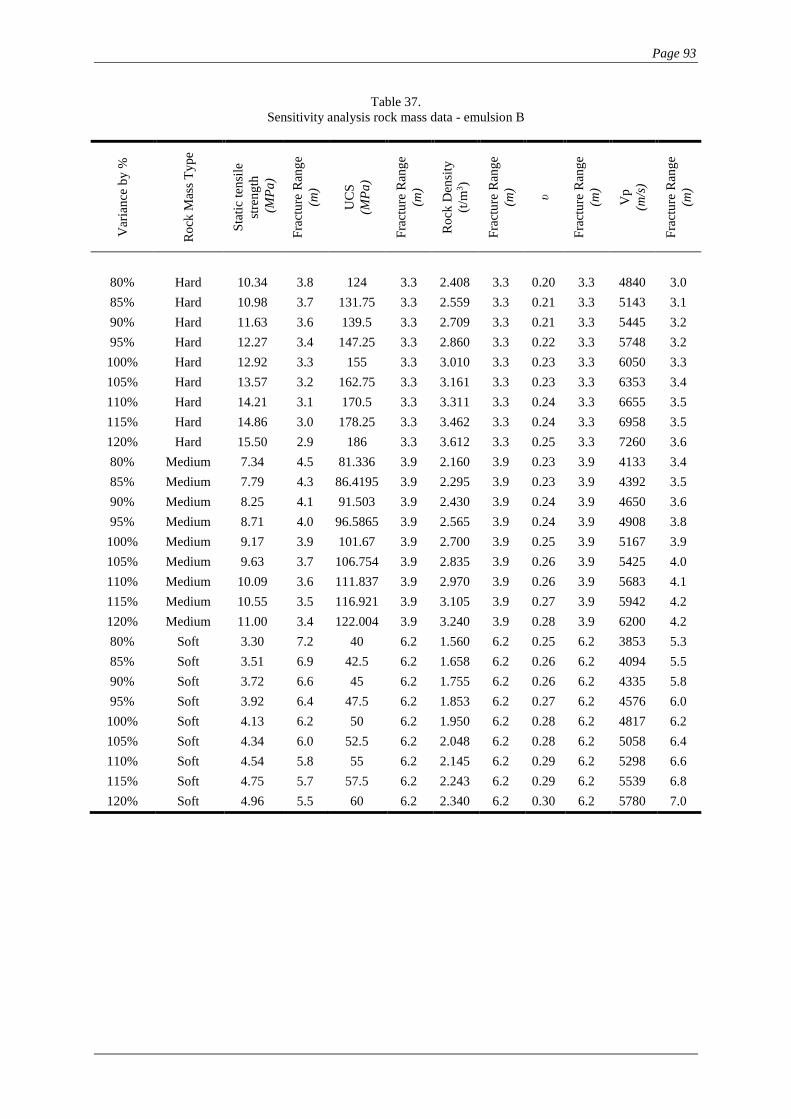
Page 93
Table 37.
Sensitivity analysis rock mass data - emulsion B
V
aria
nce
by
%
Ro
ck M
ass
Ty
pe
Sta
tic
ten
sile
stre
ng
th
(M
Pa
)
Fra
ctu
re R
ang
e
(m)
UC
S
(MP
a)
Fra
ctu
re R
ang
e
(m)
Ro
ck D
ensi
ty
(t/m
3)
Fra
ctu
re R
ang
e
(m)
υ
Fra
ctu
re R
ang
e
(m)
Vp
(m/s
)
Fra
ctu
re R
ang
e
(m)
80% Hard 10.34 3.8 124 3.3 2.408 3.3 0.20 3.3 4840 3.0
85% Hard 10.98 3.7 131.75 3.3 2.559 3.3 0.21 3.3 5143 3.1
90% Hard 11.63 3.6 139.5 3.3 2.709 3.3 0.21 3.3 5445 3.2
95% Hard 12.27 3.4 147.25 3.3 2.860 3.3 0.22 3.3 5748 3.2
100% Hard 12.92 3.3 155 3.3 3.010 3.3 0.23 3.3 6050 3.3
105% Hard 13.57 3.2 162.75 3.3 3.161 3.3 0.23 3.3 6353 3.4
110% Hard 14.21 3.1 170.5 3.3 3.311 3.3 0.24 3.3 6655 3.5
115% Hard 14.86 3.0 178.25 3.3 3.462 3.3 0.24 3.3 6958 3.5
120% Hard 15.50 2.9 186 3.3 3.612 3.3 0.25 3.3 7260 3.6
80% Medium 7.34 4.5 81.336 3.9 2.160 3.9 0.23 3.9 4133 3.4
85% Medium 7.79 4.3 86.4195 3.9 2.295 3.9 0.23 3.9 4392 3.5
90% Medium 8.25 4.1 91.503 3.9 2.430 3.9 0.24 3.9 4650 3.6
95% Medium 8.71 4.0 96.5865 3.9 2.565 3.9 0.24 3.9 4908 3.8
100% Medium 9.17 3.9 101.67 3.9 2.700 3.9 0.25 3.9 5167 3.9
105% Medium 9.63 3.7 106.754 3.9 2.835 3.9 0.26 3.9 5425 4.0
110% Medium 10.09 3.6 111.837 3.9 2.970 3.9 0.26 3.9 5683 4.1
115% Medium 10.55 3.5 116.921 3.9 3.105 3.9 0.27 3.9 5942 4.2
120% Medium 11.00 3.4 122.004 3.9 3.240 3.9 0.28 3.9 6200 4.2
80% Soft 3.30 7.2 40 6.2 1.560 6.2 0.25 6.2 3853 5.3
85% Soft 3.51 6.9 42.5 6.2 1.658 6.2 0.26 6.2 4094 5.5
90% Soft 3.72 6.6 45 6.2 1.755 6.2 0.26 6.2 4335 5.8
95% Soft 3.92 6.4 47.5 6.2 1.853 6.2 0.27 6.2 4576 6.0
100% Soft 4.13 6.2 50 6.2 1.950 6.2 0.28 6.2 4817 6.2
105% Soft 4.34 6.0 52.5 6.2 2.048 6.2 0.28 6.2 5058 6.4
110% Soft 4.54 5.8 55 6.2 2.145 6.2 0.29 6.2 5298 6.6
115% Soft 4.75 5.7 57.5 6.2 2.243 6.2 0.29 6.2 5539 6.8
120% Soft 4.96 5.5 60 6.2 2.340 6.2 0.30 6.2 5780 7.0

Page 94
Table 38.
Sensitivity analysis explosive properties data - emulsion B
Var
ian
ce b
y %
Ro
ck M
ass
Ty
pe
VO
D
(m/s
)
Fra
ctu
re R
ang
e
(m)
Ex
plo
siv
e D
ensi
ty
(kg
/m3)
Fra
ctu
re R
ang
e
(m)
Bo
reh
ole
Dia
met
er
(mm
)
Fra
ctu
re R
ang
e
(m)
80% Hard 3920 2.6 920 2.8 128 2.7
85% Hard 4165 2.8 978 3.0 136 2.8
90% Hard 4410 3.0 1035 3.1 144 3.0
95% Hard 4655 3.2 1093 3.2 152 3.1
100% Hard 4900 3.3 1150 3.3 160 3.3
105% Hard 5145 3.5 1208 3.4 168 3.5
110% Hard 5390 3.6 1265 3.5 176 3.6
115% Hard 5635 3.7 1323 3.6 184 3.8
120% Hard 5880 3.9 1380 3.8 192 4.0
80% Medium 3920 3.2 920 3.3 128 3.1
85% Medium 4165 3.4 978 3.5 136 3.3
90% Medium 4410 3.5 1035 3.6 144 3.5
95% Medium 4655 3.7 1093 3.7 152 3.7
100% Medium 4900 3.9 1150 3.9 160 3.9
105% Medium 5145 4.0 1208 4.0 168 4.1
110% Medium 5390 4.1 1265 4.1 176 4.2
115% Medium 5635 4.3 1323 4.2 184 4.4
120% Medium 5880 4.4 1380 4.4 192 4.6
80% Soft 3920 5.3 920 5.3 128 5.0
85% Soft 4165 5.6 978 5.5 136 5.3
90% Soft 4410 5.8 1035 5.7 144 5.6
95% Soft 4655 6.0 1093 5.9 152 5.9
100% Soft 4900 6.2 1150 6.1 160 6.2
105% Soft 5145 6.4 1208 6.3 168 6.5
110% Soft 5390 6.5 1265 6.5 176 6.8
115% Soft 5635 6.7 1323 6.7 184 7.1
120% Soft 5880 6.8 1380 6.9 192 7.4
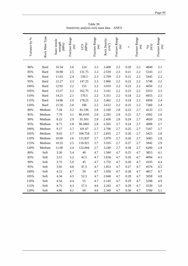
Page 95
Table 39.
Sensitivity analysis rock mass data – ANFO
V
aria
nce
by
%
Ro
ck M
ass
Ty
pe
Sta
tic
ten
sile
stre
ng
th
(MP
a)
Fra
ctu
re R
ang
e
(m)
UC
S
(MP
a)
Fra
ctu
re R
ang
e
(m)
Ro
ck D
ensi
ty
(t/m
3)
Fra
ctu
re R
ang
e
(m)
υ
Fra
ctu
re R
ang
e
(m)
Vp
(m/s
)
Fra
ctu
re R
ang
e
(m)
80% Hard 10.34 2.6 124 2.3 2.408 2.3 0.20 2.2 4840 2.1
85% Hard 10.98 2.5 131.75 2.3 2.559 2.3 0.21 2.2 5143 2.1
90% Hard 11.63 2.4 139.5 2.3 2.709 2.3 0.21 2.2 5445 2.2
95% Hard 12.27 2.3 147.25 2.3 2.860 2.2 0.22 2.2 5748 2.2
100% Hard 12.92 2.2 155 2.2 3.010 2.2 0.23 2.2 6050 2.2
105% Hard 13.57 2.2 162.75 2.2 3.161 2.2 0.23 2.2 6353 2.3
110% Hard 14.21 2.1 170.5 2.2 3.311 2.2 0.24 2.2 6655 2.3
115% Hard 14.86 2.0 178.25 2.2 3.462 2.2 0.24 2.2 6958 2.4
120% Hard 15.50 2.0 186 2.2 3.612 2.2 0.25 2.2 7260 2.4
80% Medium 7.34 3.2 81.336 2.8 2.160 2.8 0.23 2.7 4133 2.5
85% Medium 7.79 3.1 86.4195 2.8 2.295 2.8 0.23 2.7 4392 2.6
90% Medium 8.25 2.9 91.503 2.8 2.430 2.8 0.24 2.7 4650 2.6
95% Medium 8.71 2.8 96.5865 2.8 2.565 2.7 0.24 2.7 4908 2.7
100% Medium 9.17 2.7 101.67 2.7 2.700 2.7 0.25 2.7 5167 2.7
105% Medium 9.63 2.7 106.754 2.7 2.835 2.7 0.26 2.7 5425 2.8
110% Medium 10.09 2.6 111.837 2.7 2.970 2.7 0.26 2.7 5683 2.8
115% Medium 10.55 2.5 116.921 2.7 3.105 2.7 0.27 2.7 5942 2.9
120% Medium 11.00 2.4 122.004 2.7 3.240 2.7 0.28 2.7 6200 2.9
80% Soft 3.30 5.4 40 4.7 1.560 4.7 0.25 4.7 3853 4.1
85% Soft 3.51 5.2 42.5 4.7 1.658 4.7 0.26 4.7 4094 4.3
90% Soft 3.72 5.0 45 4.7 1.755 4.7 0.26 4.7 4335 4.4
95% Soft 3.92 4.8 47.5 4.7 1.853 4.7 0.27 4.7 4576 4.5
100% Soft 4.13 4.7 50 4.7 1.950 4.7 0.28 4.7 4817 4.7
105% Soft 4.34 4.5 52.5 4.7 2.048 4.7 0.28 4.7 5058 4.8
110% Soft 4.54 4.4 55 4.7 2.145 4.7 0.29 4.7 5298 4.9
115% Soft 4.75 4.3 57.5 4.6 2.243 4.7 0.29 4.7 5539 5.0
120% Soft 4.96 4.1 60 4.6 2.340 4.7 0.30 4.7 5780 5.1
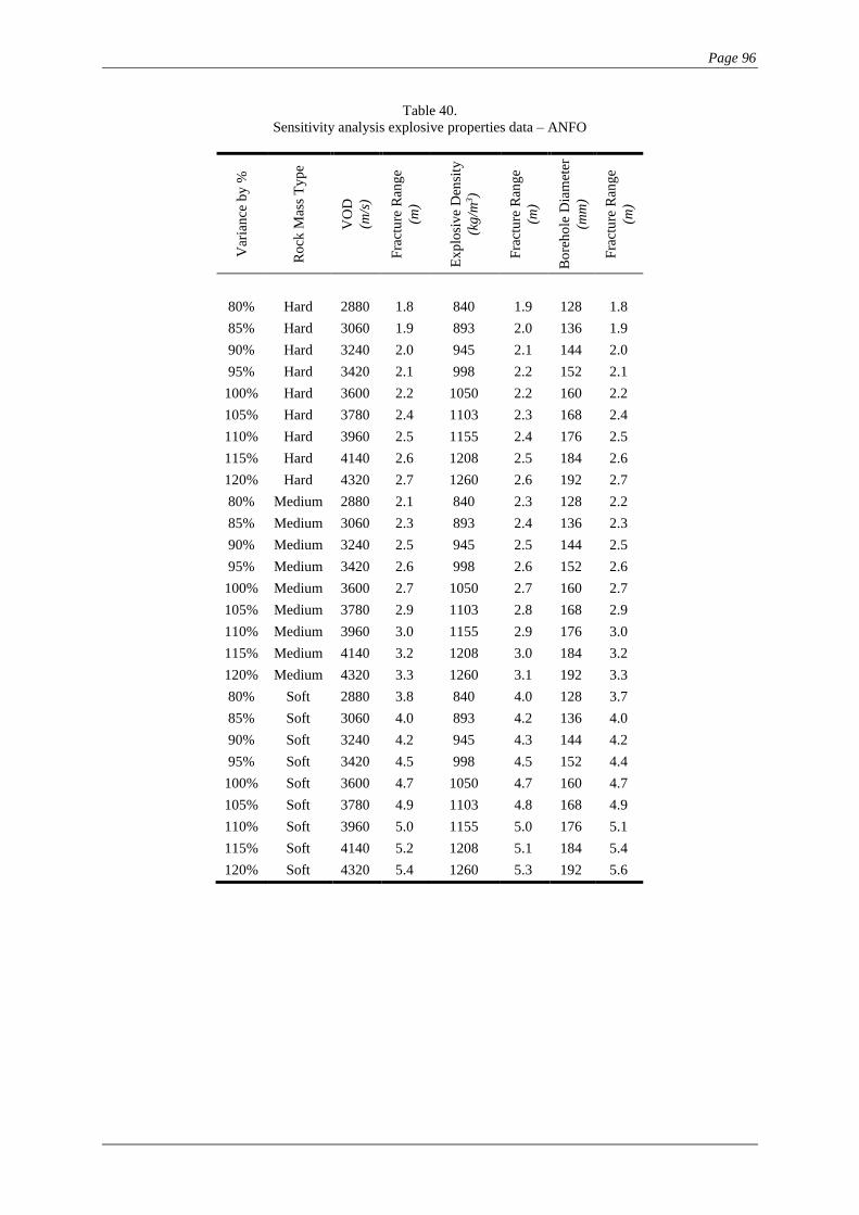
Page 96
Table 40.
Sensitivity analysis explosive properties data – ANFO
Var
ian
ce b
y %
Ro
ck M
ass
Ty
pe
VO
D
(m/s
)
Fra
ctu
re R
ang
e
(m)
Ex
plo
siv
e D
ensi
ty
(kg
/m3)
Fra
ctu
re R
ang
e
(m)
Bo
reh
ole
Dia
met
er
(mm
)
Fra
ctu
re R
ang
e
(m)
80% Hard 2880 1.8 840 1.9 128 1.8
85% Hard 3060 1.9 893 2.0 136 1.9
90% Hard 3240 2.0 945 2.1 144 2.0
95% Hard 3420 2.1 998 2.2 152 2.1
100% Hard 3600 2.2 1050 2.2 160 2.2
105% Hard 3780 2.4 1103 2.3 168 2.4
110% Hard 3960 2.5 1155 2.4 176 2.5
115% Hard 4140 2.6 1208 2.5 184 2.6
120% Hard 4320 2.7 1260 2.6 192 2.7
80% Medium 2880 2.1 840 2.3 128 2.2
85% Medium 3060 2.3 893 2.4 136 2.3
90% Medium 3240 2.5 945 2.5 144 2.5
95% Medium 3420 2.6 998 2.6 152 2.6
100% Medium 3600 2.7 1050 2.7 160 2.7
105% Medium 3780 2.9 1103 2.8 168 2.9
110% Medium 3960 3.0 1155 2.9 176 3.0
115% Medium 4140 3.2 1208 3.0 184 3.2
120% Medium 4320 3.3 1260 3.1 192 3.3
80% Soft 2880 3.8 840 4.0 128 3.7
85% Soft 3060 4.0 893 4.2 136 4.0
90% Soft 3240 4.2 945 4.3 144 4.2
95% Soft 3420 4.5 998 4.5 152 4.4
100% Soft 3600 4.7 1050 4.7 160 4.7
105% Soft 3780 4.9 1103 4.8 168 4.9
110% Soft 3960 5.0 1155 5.0 176 5.1
115% Soft 4140 5.2 1208 5.1 184 5.4
120% Soft 4320 5.4 1260 5.3 192 5.6
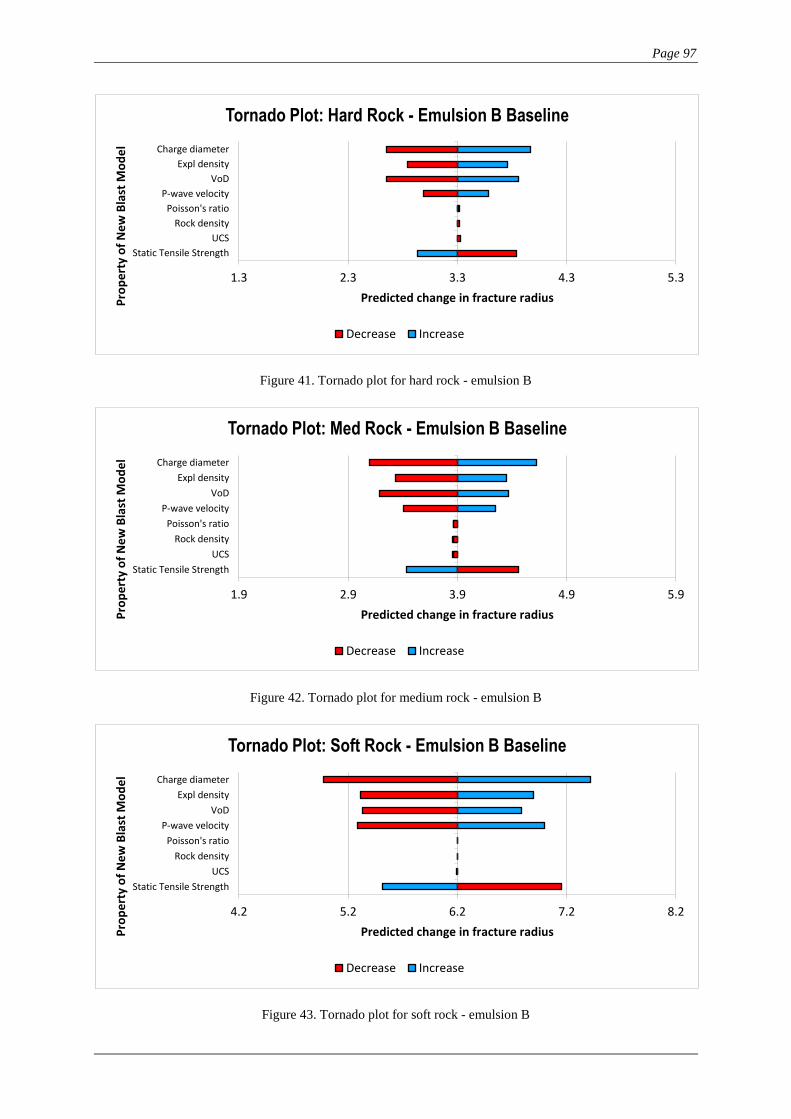
Page 97
Figure 41. Tornado plot for hard rock - emulsion B
Figure 42. Tornado plot for medium rock - emulsion B
Figure 43. Tornado plot for soft rock - emulsion B
1.3 2.3 3.3 4.3 5.3
Static Tensile Strength
UCS
Rock density
Poisson's ratio
P-wave velocity
VoD
Expl density
Charge diameter
Predicted change in fracture radiusPro
pe
rty
of
Ne
w B
last
Mo
de
lTornado Plot: Hard Rock - Emulsion B Baseline
Decrease Increase
1.9 2.9 3.9 4.9 5.9
Static Tensile Strength
UCS
Rock density
Poisson's ratio
P-wave velocity
VoD
Expl density
Charge diameter
Predicted change in fracture radiusPro
pe
rty
of
Ne
w B
last
Mo
de
l
Tornado Plot: Med Rock - Emulsion B Baseline
Decrease Increase
4.2 5.2 6.2 7.2 8.2
Static Tensile Strength
UCS
Rock density
Poisson's ratio
P-wave velocity
VoD
Expl density
Charge diameter
Predicted change in fracture radiusPro
pe
rty
of
Ne
w B
last
Mo
de
l
Tornado Plot: Soft Rock - Emulsion B Baseline
Decrease Increase
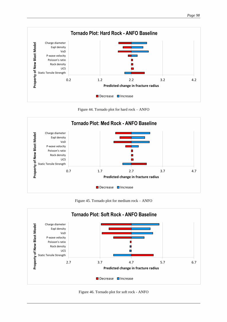
Page 98
Figure 44. Tornado plot for hard rock – ANFO
Figure 45. Tornado plot for medium rock – ANFO
Figure 46. Tornado plot for soft rock - ANFO
0.2 1.2 2.2 3.2 4.2
Static Tensile Strength
UCS
Rock density
Poisson's ratio
P-wave velocity
VoD
Expl density
Charge diameter
Predicted change in fracture radiusPro
pe
rty
of
Ne
w B
last
Mo
de
lTornado Plot: Hard Rock - ANFO Baseline
Decrease Increase
0.7 1.7 2.7 3.7 4.7
Static Tensile Strength
UCS
Rock density
Poisson's ratio
P-wave velocity
VoD
Expl density
Charge diameter
Predicted change in fracture radiusPro
pe
rty
of
Ne
w B
last
Mo
de
l
Tornado Plot: Med Rock - ANFO Baseline
Decrease Increase
2.7 3.7 4.7 5.7 6.7
Static Tensile Strength
UCS
Rock density
Poisson's ratio
P-wave velocity
VoD
Expl density
Charge diameter
Predicted change in fracture radiusPro
pe
rty
of
Ne
w B
last
Mo
de
l
Tornado Plot: Soft Rock - ANFO Baseline
Decrease Increase
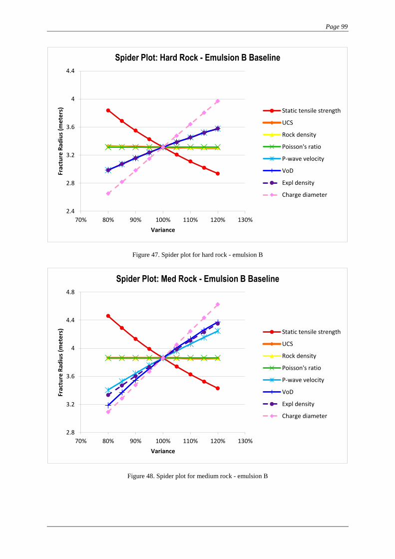
Page 99
Figure 47. Spider plot for hard rock - emulsion B
Figure 48. Spider plot for medium rock - emulsion B
2.4
2.8
3.2
3.6
4
4.4
70% 80% 90% 100% 110% 120% 130%
Frac
ture
Rad
ius
(me
ters
)
Variance
Spider Plot: Hard Rock - Emulsion B Baseline
Static tensile strength
UCS
Rock density
Poisson's ratio
P-wave velocity
VoD
Expl density
Charge diameter
2.8
3.2
3.6
4
4.4
4.8
70% 80% 90% 100% 110% 120% 130%
Frac
ture
Rad
ius
(me
ters
)
Variance
Spider Plot: Med Rock - Emulsion B Baseline
Static tensile strength
UCS
Rock density
Poisson's ratio
P-wave velocity
VoD
Expl density
Charge diameter
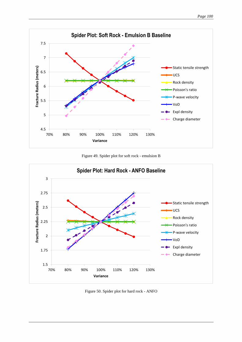
Page 100
Figure 49. Spider plot for soft rock - emulsion B
Figure 50. Spider plot for hard rock - ANFO
4.5
5
5.5
6
6.5
7
7.5
70% 80% 90% 100% 110% 120% 130%
Frac
ture
Rad
ius
(me
ters
)
Variance
Spider Plot: Soft Rock - Emulsion B Baseline
Static tensile strength
UCS
Rock density
Poisson's ratio
P-wave velocity
VoD
Expl density
Charge diameter
1.5
1.75
2
2.25
2.5
2.75
3
70% 80% 90% 100% 110% 120% 130%
Frac
ture
Rad
ius
(me
ters
)
Variance
Spider Plot: Hard Rock - ANFO Baseline
Static tensile strength
UCS
Rock density
Poisson's ratio
P-wave velocity
VoD
Expl density
Charge diameter
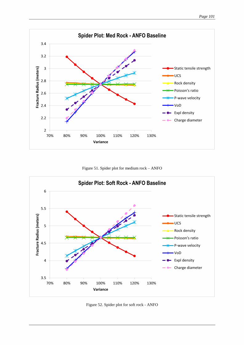
Page 101
Figure 51. Spider plot for medium rock – ANFO
Figure 52. Spider plot for soft rock - ANFO
2
2.2
2.4
2.6
2.8
3
3.2
3.4
70% 80% 90% 100% 110% 120% 130%
Frac
ture
Rad
ius
(me
ters
)
Variance
Spider Plot: Med Rock - ANFO Baseline
Static tensile strength
UCS
Rock density
Poisson's ratio
P-wave velocity
VoD
Expl density
Charge diameter
3.5
4
4.5
5
5.5
6
70% 80% 90% 100% 110% 120% 130%
Frac
ture
Rad
ius
(me
ters
)
Variance
Spider Plot: Soft Rock - ANFO Baseline
Static tensile strength
UCS
Rock density
Poisson's ratio
P-wave velocity
VoD
Expl density
Charge diameter
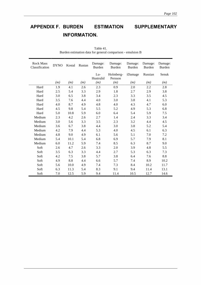
Page 102
APPENDIX F. BURDEN ESTIMATION SUPPLEMENTARY
INFORMATION.
Table 41.
Burden estimation data for general comparison - emulsion B
Rock Mass
Classification DYNO Kostal Rustan
Damage:
Burden
Damage:
Burden
Damage:
Burden
Damage:
Burden
Damage:
Burden
(m)
(m)
(m)
Lu-
Hustrulid
(m)
Holmberg-
Persson
(m)
iDamage
(m)
Russian
(m)
Senuk
(m)
Hard 1.9 4.1 2.6 2.3 0.9 2.0 2.2 2.8
Hard 2.5 5.4 3.3 2.9 1.8 2.7 2.9 3.8
Hard 3.0 6.5 3.8 3.4 2.3 3.3 3.5 4.5
Hard 3.5 7.6 4.4 4.0 3.0 3.8 4.1 5.3
Hard 4.0 8.7 4.9 4.8 4.0 4.3 4.7 6.0
Hard 4.5 9.8 5.4 5.5 5.2 4.9 5.3 6.8
Hard 5.0 10.8 5.9 6.0 6.4 5.4 5.9 7.5
Medium 2.3 4.2 2.6 2.7 1.4 2.4 3.3 3.4
Medium 3.0 5.6 3.3 3.5 2.3 3.2 4.4 4.5
Medium 3.6 6.7 3.8 4.4 3.0 3.8 5.2 5.4
Medium 4.2 7.9 4.4 5.3 4.0 4.5 6.1 6.3
Medium 4.8 9.0 4.9 6.1 5.6 5.1 7.0 7.2
Medium 5.4 10.1 5.4 6.8 6.9 5.7 7.9 8.1
Medium 6.0 11.2 5.9 7.4 8.5 6.3 8.7 9.0
Soft 2.6 4.7 2.6 3.3 2.0 3.9 4.8 5.5
Soft 3.5 6.3 3.3 4.4 2.7 5.3 6.3 7.3
Soft 4.2 7.5 3.8 5.7 3.8 6.4 7.6 8.8
Soft 4.9 8.8 4.4 6.6 5.7 7.4 8.9 10.2
Soft 5.6 10.0 4.9 7.4 7.3 8.4 10.2 11.7
Soft 6.3 11.3 5.4 8.3 9.1 9.4 11.4 13.1
Soft 7.0 12.5 5.9 9.4 11.4 10.5 12.7 14.6
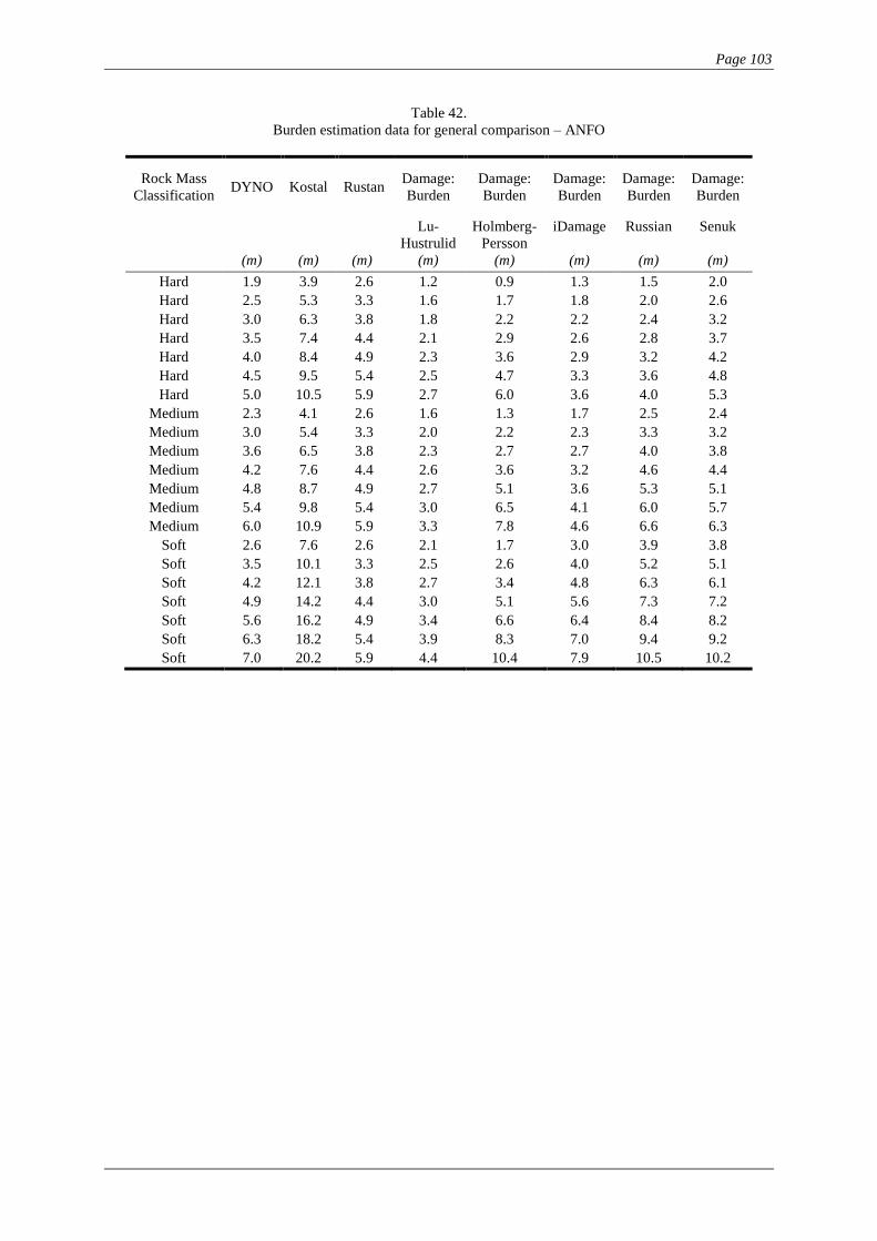
Page 103
Table 42.
Burden estimation data for general comparison – ANFO
Rock Mass
Classification DYNO Kostal Rustan
Damage:
Burden
Damage:
Burden
Damage:
Burden
Damage:
Burden
Damage:
Burden
(m) (m) (m)
Lu-
Hustrulid
(m)
Holmberg-
Persson
(m)
iDamage
(m)
Russian
(m)
Senuk
(m)
Hard 1.9 3.9 2.6 1.2 0.9 1.3 1.5 2.0
Hard 2.5 5.3 3.3 1.6 1.7 1.8 2.0 2.6
Hard 3.0 6.3 3.8 1.8 2.2 2.2 2.4 3.2
Hard 3.5 7.4 4.4 2.1 2.9 2.6 2.8 3.7
Hard 4.0 8.4 4.9 2.3 3.6 2.9 3.2 4.2
Hard 4.5 9.5 5.4 2.5 4.7 3.3 3.6 4.8
Hard 5.0 10.5 5.9 2.7 6.0 3.6 4.0 5.3
Medium 2.3 4.1 2.6 1.6 1.3 1.7 2.5 2.4
Medium 3.0 5.4 3.3 2.0 2.2 2.3 3.3 3.2
Medium 3.6 6.5 3.8 2.3 2.7 2.7 4.0 3.8
Medium 4.2 7.6 4.4 2.6 3.6 3.2 4.6 4.4
Medium 4.8 8.7 4.9 2.7 5.1 3.6 5.3 5.1
Medium 5.4 9.8 5.4 3.0 6.5 4.1 6.0 5.7
Medium 6.0 10.9 5.9 3.3 7.8 4.6 6.6 6.3
Soft 2.6 7.6 2.6 2.1 1.7 3.0 3.9 3.8
Soft 3.5 10.1 3.3 2.5 2.6 4.0 5.2 5.1
Soft 4.2 12.1 3.8 2.7 3.4 4.8 6.3 6.1
Soft 4.9 14.2 4.4 3.0 5.1 5.6 7.3 7.2
Soft 5.6 16.2 4.9 3.4 6.6 6.4 8.4 8.2
Soft 6.3 18.2 5.4 3.9 8.3 7.0 9.4 9.2
Soft 7.0 20.2 5.9 4.4 10.4 7.9 10.5 10.2
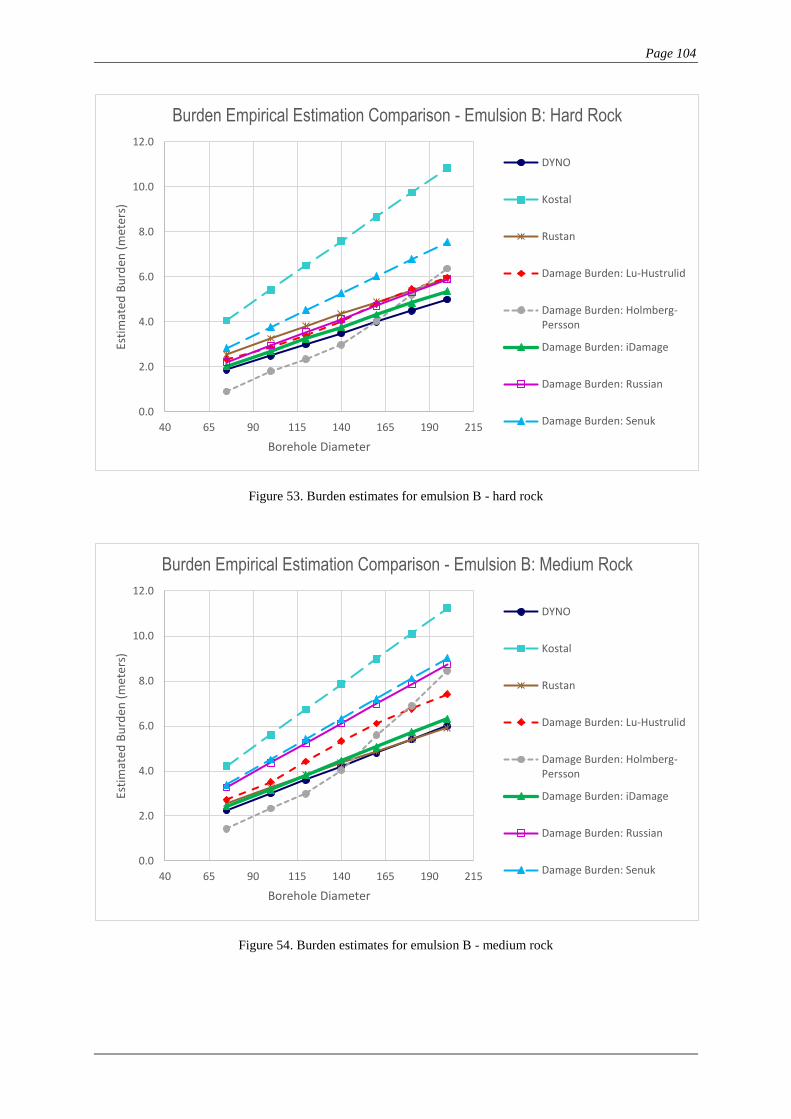
Page 104
Figure 53. Burden estimates for emulsion B - hard rock
Figure 54. Burden estimates for emulsion B - medium rock
0.0
2.0
4.0
6.0
8.0
10.0
12.0
40 65 90 115 140 165 190 215
Esti
mat
ed B
urd
en (
met
ers)
Borehole Diameter
Burden Empirical Estimation Comparison - Emulsion B: Hard Rock
DYNO
Kostal
Rustan
Damage Burden: Lu-Hustrulid
Damage Burden: Holmberg-Persson
Damage Burden: iDamage
Damage Burden: Russian
Damage Burden: Senuk
0.0
2.0
4.0
6.0
8.0
10.0
12.0
40 65 90 115 140 165 190 215
Esti
mat
ed B
urd
en (
met
ers)
Borehole Diameter
Burden Empirical Estimation Comparison - Emulsion B: Medium Rock
DYNO
Kostal
Rustan
Damage Burden: Lu-Hustrulid
Damage Burden: Holmberg-Persson
Damage Burden: iDamage
Damage Burden: Russian
Damage Burden: Senuk
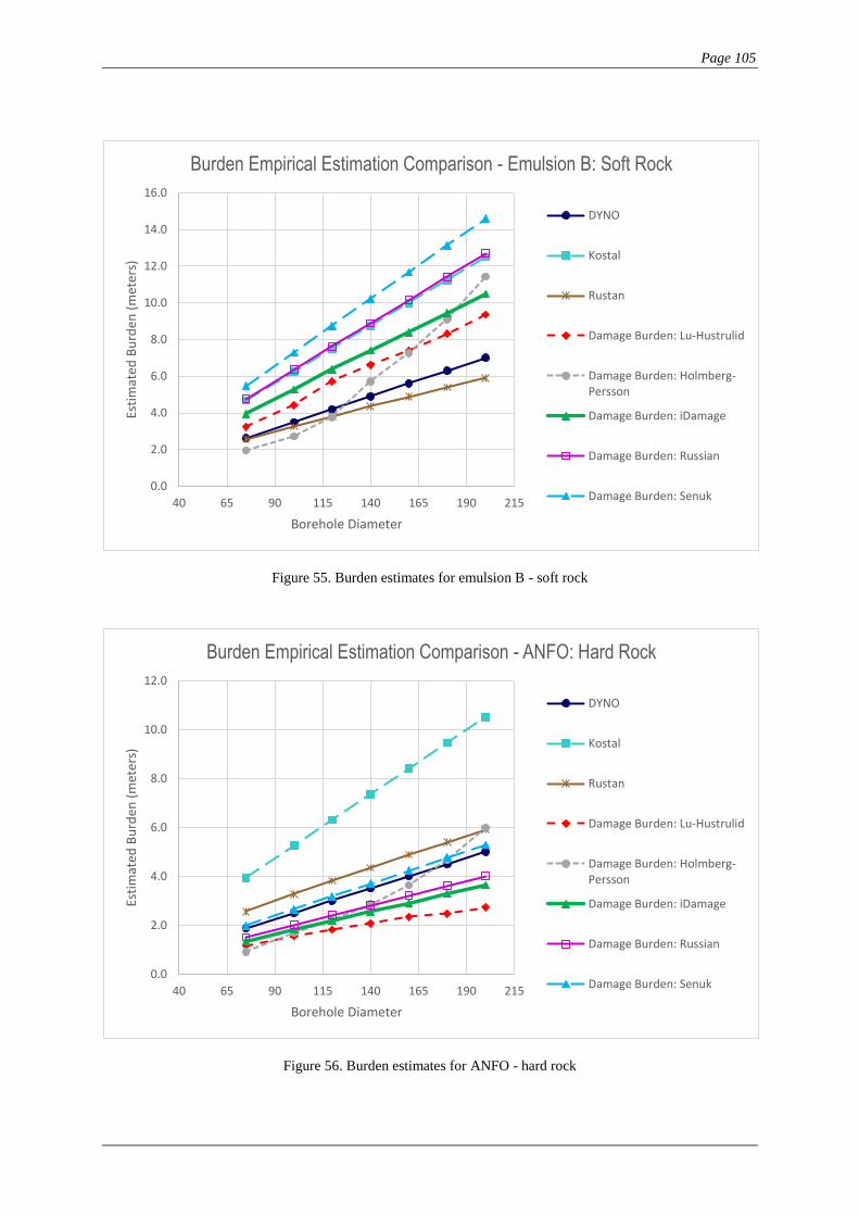
Page 105
Figure 55. Burden estimates for emulsion B - soft rock
Figure 56. Burden estimates for ANFO - hard rock
0.0
2.0
4.0
6.0
8.0
10.0
12.0
14.0
16.0
40 65 90 115 140 165 190 215
Esti
mat
ed B
urd
en (
met
ers)
Borehole Diameter
Burden Empirical Estimation Comparison - Emulsion B: Soft Rock
DYNO
Kostal
Rustan
Damage Burden: Lu-Hustrulid
Damage Burden: Holmberg-Persson
Damage Burden: iDamage
Damage Burden: Russian
Damage Burden: Senuk
0.0
2.0
4.0
6.0
8.0
10.0
12.0
40 65 90 115 140 165 190 215
Esti
mat
ed B
urd
en (
met
ers)
Borehole Diameter
Burden Empirical Estimation Comparison - ANFO: Hard Rock
DYNO
Kostal
Rustan
Damage Burden: Lu-Hustrulid
Damage Burden: Holmberg-Persson
Damage Burden: iDamage
Damage Burden: Russian
Damage Burden: Senuk
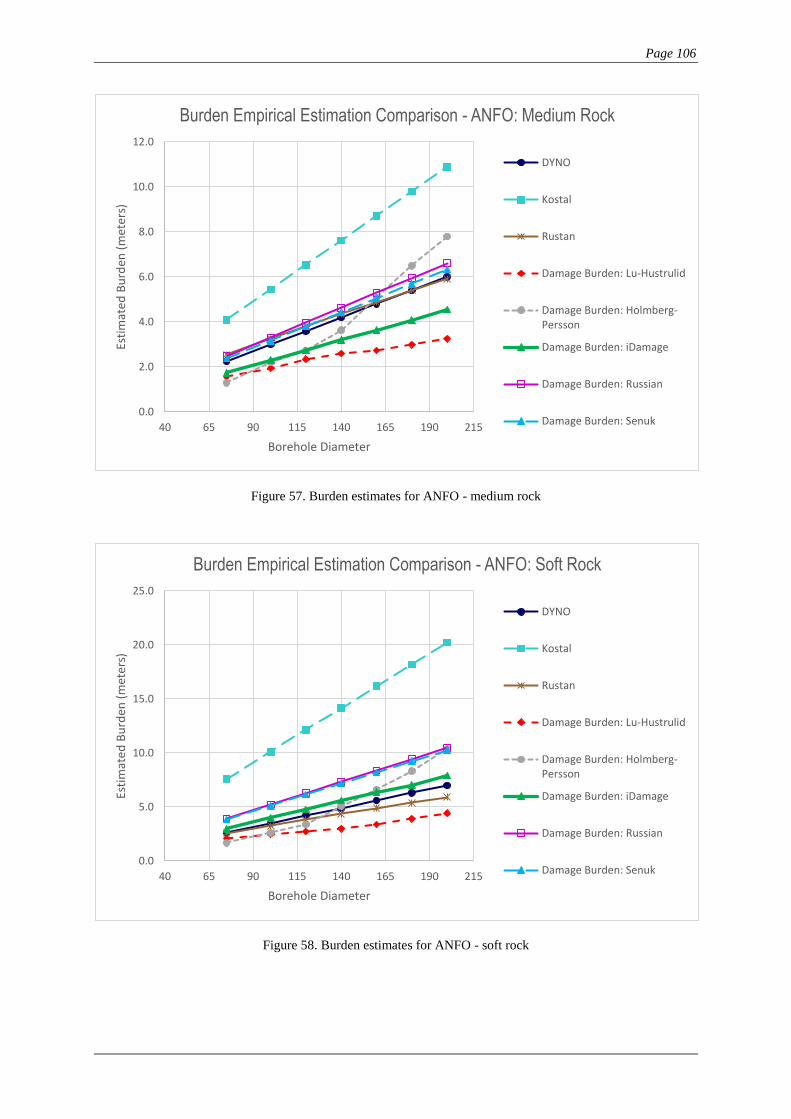
Page 106
Figure 57. Burden estimates for ANFO - medium rock
Figure 58. Burden estimates for ANFO - soft rock
0.0
2.0
4.0
6.0
8.0
10.0
12.0
40 65 90 115 140 165 190 215
Esti
mat
ed B
urd
en (
met
ers)
Borehole Diameter
Burden Empirical Estimation Comparison - ANFO: Medium Rock
DYNO
Kostal
Rustan
Damage Burden: Lu-Hustrulid
Damage Burden: Holmberg-Persson
Damage Burden: iDamage
Damage Burden: Russian
Damage Burden: Senuk
0.0
5.0
10.0
15.0
20.0
25.0
40 65 90 115 140 165 190 215
Esti
mat
ed B
urd
en (
met
ers)
Borehole Diameter
Burden Empirical Estimation Comparison - ANFO: Soft Rock
DYNO
Kostal
Rustan
Damage Burden: Lu-Hustrulid
Damage Burden: Holmberg-Persson
Damage Burden: iDamage
Damage Burden: Russian
Damage Burden: Senuk