ON HISTORICAL HOUSEHOLD BUDGETS

Brian A’Hearn, Nicola Amendola, and

Giovanni Vecchi

U N I V E R S I T Y O F O X F O R D

Discussion Papers in Economic and Social History

Number 144, June 2016

1

On Historical Household Budgets

Brian A’Hearn Pembroke College, University of Oxford

Nicola Amendola

Dept. of Economics and Finance, University of Rome “Tor Vergata”

Giovanni Vecchi1 Dept. of Economics and Finance, University of Rome “Tor Vergata”

May 2016

Abstract

The paper argues that household budgets are the best starting point for investigating a

number of big questions related to the evolution of the living standards during the last

two-three centuries. If one knows where to look, historical family budgets are more

abundant than might be suspected. And statistical techniques have been developed to

handle the associated problems of small, incomplete, and unrepresentative samples. We

introduce the Historical Household Budgets (HHB) Project, aimed at gathering data and

sources, but also at creating an informational infrastructure that provides i) reliable

storage and easy access to historical family budget data, along with ii) tools to configure

the data as it is entered so as to harmonise it with present-day surveys.

Keywords: household budgets; household budget surveys; living standards; inequality;

poverty; survey; globalization; purchasing power parities; grouped data; post-

stratification.

JEL classification: N30, I31, I32, C81, C83, D60, D63, O12, O15.

1 Author for correspondence: Giovanni Vecchi, Department of Economics and Finance, University of Rome “Tor Vergata”. E-mail: giovanni.vecchi@uniroma2.it. The paper is part of a broader research project supported by the Institute for New Economic Thinking (INET), Grant #INO15-00026. Details are available at http://hhbproject.com.

3

1 Introduction

Like a fairy-tale giant lifting the roof of a house to peer inside, economic historians

wish they could see into the lives of families of the past. For important questions can

only be answered with detailed evidence about individual households. This is obvious

when interest centers on the intra-household allocation of resources, that is, questions of

whose consumption was protected when times were tough: the primary breadwinner,

the children, males? It is equally true of other questions naturally posed at the level of

the household. Was poverty a feature of the life cycle, something episodic, or a chronic

condition? How did parents choose between their children’s involvement in education,

home production, and outside employment? Who benefited from rural-urban migration?

On what margins did families react to shocks like a decline in wages: hours worked,

home production, quality of diet or dwelling, wealth accumulation?

Convincing answers even to questions of a more macroeconomic nature require

disaggregated welfare indicators. We are increasingly aware that the great forces of our

era – globalisation and technical change – create losers as well as winners (O’Rourke

and Williamson, 1999). We are increasingly concerned about rising inequality and its

political implications (Bourguignon, 2015; Milanovic, 2016). We worry about future

trends and whether policy is capable of making a difference (Piketty, 2014; Atkinson,

2015). This is true within and between countries, for the rich world and developing

nations (Deaton, 2013).

Modern economists take household-level data for granted, but do they exist for times

past? In this article we show that historical data on families are more than just a fairy

tale. Household budgets, in particular, are available for more countries, for a longer

span of time (back to the mid-nineteenth century and beyond), and in much greater

numbers than is generally supposed. To be sure, they are not always easy to use:

particular collections of budgets are rarely representative, seldom directly comparable

across sources. But the tools of the modern welfare analyst can mitigate these problems

in historical contexts too. There is thus a real opportunity to give a decisive boost to

historical research on both the microeconomics of households and the macro dynamics

of welfare; this is the case we make in this article. In Sections 2 and 3, we describe

modern and historical household budgets, respectively, with a very brief review of their

previous use in economic history. The focus then narrows to our own area of interest,

4

the long-run evolution of living standards, poverty, and inequality. In Section 4 we

review existing historical research on these issues. Section 5 addresses technical

problems arising in work with historical family budgets and in welfare comparisons

over time and across countries. We outline our new Historical Household Budgets

initiative in Section 6, and present some preliminary results for the Italian case in

Section 7. We conclude our manifesto with a call to arms in Section 8.

2 In praise of modern household budgets

In current usage, a household budget is an accounting schedule that sets out the incomes

and expenditures of a household with reference to a given period of time.4 Many people

keep household accounts, often in an informal way, in order to keep an eye on the

family’s incomes and expenditures. Besides being a domestic tool in citizens’ private

lives, household budgets play a fundamental role in modern economics and statistics

(Deaton, 1997). Each year, millions of individuals are interviewed the world over by an

army of interviewers sent by national statistical offices, independent research institutes,

and other organizations. In many countries, participation in household budget surveys is

mandatory by law. What are all these data on household budgets for, and who uses

them?

A convenient starting point is to note that household budgets, in contrast to other

statistics, let us see how families respond to the economic environment. Wage data or

unemployment figures might show us that, say, industrial workers’ living standards are

under pressure. But this tells us little about how their families are affected or how they

react. They might switch consumption from expensive meat to cheap starches, cut

health care expenditures, or produce more at home for their own consumption; they

might keep children out of school and put them to work; a stay-at-home spouse might

take up market employment; the family might move to a smaller house, take in lodgers,

or spend less on fuel; the head of household may work more days per year by taking on

a secondary employment; they might maintain consumption by drawing down family

4 Households and families are the basic units of analysis here; they are not the same thing. A household is composed of one or more people who share the same dwelling, and not all households contain families. In turn, a family is defined as those members of the household who are related, to a specified degree, through blood, adoption or marriage. Currently, no single definition has general use around the world.

5

savings or mobilising community resources. Wage data tell us none of this. Even

income data would fail to tell us how and why annual incomes were maintained despite

falling wages. It is only when we know about consumption patterns, wealth and savings,

housing, labour market participation of family members, and so on that we can fully

understand a) the level and dynamics of family welfare, and b) the strategies families

use to cope with economic adversity.

For the academic community, international organizations, and governments, household

budgets are an essential input for economic analyses.5 Household incomes and/or

expenditures are used to measure economic welfare. A household’s, or an individual’s,

standard of living encompasses health status, education, freedom, access to basic

services; it is more than just money. Still, if we seek one indicator, then consumption

may be the best available approximation to utility, which is the starting point for how

economists think about household behaviour and about welfare (Deaton and Grosh,

1998). Household budgets are therefore essential for analyzing the distribution of

welfare and understanding its determinants.

More prosaically, household budgets are a foundation for estimates of private

consumption, the most important component (55-60%) of an expenditure-based

calculation of GDP (Lequiller and Blades, 2006: ch. 6). In many countries, household

budgets are an important input into construction of the national income and product

accounts. In other cases, they serve as a useful check on the plausibility of the official

figures. Household budgets are the key to official estimates of inflation as well, for it is

the consumption patterns that they reveal which provide the weights needed to compute

a consumer price index, or alternatively a spatial price index measuring geographic

variation in the cost of living (ILO, 2004). Detailed information on the consumption

patterns of poor families is indispensable in identifying the minimum expenditure

required to reach a socially defined acceptable standard of living, in other words an

absolute poverty line.

Household budget data are similarly important in policy evaluation. They are required

to calibrate the models used in microsimulation studies of, for example, how the labour

supply of parents changes in response to changes in the tax-benefit system (Figari, 5 Of course the composition of household expenditure and its development over time interest the private sector too. They reveal the evolution of consumer tastes and preferences, i.e. the market that producers face, and are the key to producing accurate forecasts of demand (Thomas, 1987).

6

Paulus and Sutherland, 2014). The most important international agencies – from the

United Nations to the World Bank – provide technical assistance to countries requesting

it in order to design and implement surveys on household budgets: a key element for

establishing development plans and for gaining access to international financing

(Deaton, 1997).

As hinted earlier, an ideal conception of the standard of living would comprise more

than just current consumption levels. It is disaggregated, family-level data that allow

analysts to go further and adopt a multidimensional approach to welfare. Composite

indices are a popular implementation of this approach (Anand and Sen, 1994), but have

been shown to be deeply problematic (Fleurbaey, 2009; Amendola et. al. 2016), and fail

to take account of the distribution of their constituent indicators. Sufficiently

comprehensive family-level data also allow us to shift the analysis from final

achievements such as consumption to opportunities (Peragine, 2004). Another

broadening of our conception of living standards is to consider vulnerability to poverty,

which introduces the role of risk and the household’s capacity to mitigate it (Dercon,

2004). Again it is household-level data, ideally with a longitudinal dimension, that are

needed to give empirical content to this idea.

What of the collection of household budget data? Modern surveys pay particular

attention to two criteria: i) statistical representativeness, that is the units in the sample

(e.g. households, individuals, etc.) are selected through a probabilistic sampling

mechanism that ensures the data are representative of the target population (Levy and

Lemeshow, 1999); and ii) consistency of interpersonal comparisons, that is variable

definitions that ensure comparability across units (households or individuals) – and that

are theoretically grounded (Deaton and Zaidi, 2002). Virtually all countries in the world

conduct cross-section and longitudinal surveys on a regular basis for the purposes

discussed in this section. On the theoretical side, most economists would not hesitate to

argue that household budget surveys represent a “first best”.6 As with any source, they

must be used with care and an awareness of their limitations, but they are the

benchmark against which other data are compared.

6 This does not imply that they are perfect. Atkinson (2015: 48), among others, discusses their limitations. Meyer, Mok and Sullivan (2015) have argued that household surveys are in crisis, threatened by declining accuracy due to reduced cooperation of respondents. See also Burkhauser et al. (2016).

7

3 Household budgets in history

Household budgets are not a recent invention; Cicero (106 BC – 43 BC) tells us that in

ancient Rome citizens habitually kept two kinds of accounts: a sort of first entry (called

adversaria) in which they hurriedly jotted down their everyday transactions, and a real

book of expenditures (the codex accepti et expensi) in which the adversaria notes were

properly organized on a monthly basis (Smith, 1873: 17). None of these documents has

come down to us except in the form of indirect references in the letters of Cicero and

other Latin writers, but they clearly testify as to how deeply rooted in the past the habit

of family bookkeeping is (Chianese and Vecchi, 2016).

Nor do household budgets seem limited by narrow geographic boundaries. Western

Europe and the North America have a well-known and strong tradition (Stigler, 1954;

Bales, Bulmer and Sklar, 1991; Vecchi, 2016, 2011). North European countries have

“data to die for” (see Jäntti, 2006; Saaritsa, forthcoming; Öberg, forthcoming). In the

United States, studies on the living standards of the population were carried out on a

large scale well before the advent of modern surveys: Eaton and Harrison (1930) listed

2,775 surveys between 1907 and 1908 (Stapleford, 2009), while earlier initiatives have

been discussed in Converse (1987)7. Roberts (forthcoming) documents the many

sources available for other so-called western offshoots (particularly Canada, Australia

and New Zealand).

Moving east, we find in Russia perhaps the most impressive trove of historical

household budgets. These derive from the extraordinary efforts of local government

(zemstvo, pl. -a) statisticians, who collected hundreds of thousands of peasant household

budgets in the late nineteenth and early twentieth centuries (Seneta, 1985; Darrow,

2000). In carrying out tax assessments, zemstvo statisticians were also tasked with

collecting data suitable to the development of informed policies for rural development.

Fedor Andreevich Shcherbina (1849-1936), head of the Statistical Bureau of the

Voronezh Zemstvo, near the northeast border of modern Ukraine, believed that only a

household-by-household examination could do justice to the heterogeneity of Russia’s

rural economy. Shcherbina’s studies, which were emulated by his zemstvo colleagues

across the Empire, were used intensively by Lenin (Kotz and Seneta, 1990), and more

7 Relatively little is known about Latin American countries. For Mexico, López-Alonso (2012: 63-64) maintains that there are insufficient household budget data for the period prior to 1957.

8

recently by Field (1989) and Lindert and Nafziger (2012). Much of the original

microdata is now available – already digitized – to interested scholars.

Proceeding further east, historical family budgets are found in China (Fang, Wailes and

Cramer, 1998), India, as well as in Japan. In the latter country, their appearance dates

back to the Edo period (Ogura, 1982), though most sources refer to the Meji and Taishō

periods. It is worth noting that in Japan, perhaps more than in other countries, household

budgets were rooted in the national culture and formed a part of social habits well

before the modern survey era. Signs of their presence in the cultural life of the populace

are everywhere. In the magazine Fujin no Tomo (The Women’s Friend, est. 1911), Hani

Motoko (1873-1957) published a set of household finance ledgers (kakeibo),

encouraging women to rationalize management of the household (Komori, 2007). The

diffusion and success of the kakeibo on a national scale was astonishing – “Readers

eagerly welcomed those articles as ‘helpful’, ‘convenient’ and ‘interesting’, and the

magazine became one of the most popular magazines among Japanese women” (Hiroko,

2004: 55-56).8 It is no accident that large-scale surveys on household income and

expenditures were promoted by Statistics Bureau of Japan as early as 1926 (Smitka,

1998).

Finally, Africa. In 2010, Shanta Devarajan, chief economist for the African region at the

World Bank, gave a keynote speech deploring “Africa’s statistical tragedy”, that is, a

chronic “weak capacity in countries to collect, manage, and disseminate data”

(Devarajan, 2013: S12). Does Devarajan’s critique apply equally to African history?

From this angle, Africa remains a largely unexplored continent. With reference to the

20th and 21st centuries Jerven (2015) has taken up the challenge by investigating the

history of measurement for selected countries. Serra (2014) has focused on Ghana,

Marivoet and De Herdt (2015) on the Democratic Republic of Congo, Davie (2015) on

South Africa. Much more is available (ILO, 1926, 1949, 1961; Woodbury 1940), even

if currently filed under “research agenda for the future”. We will return to this issue in

Section 7.

8 Kakeibo have survived the test of time and reached global fame. When writing this article, Italian translations of kakeibo could be seen on display among the bestsellers at the main bookshop of the Rome airport. Internet bookshops too are well stocked.

9

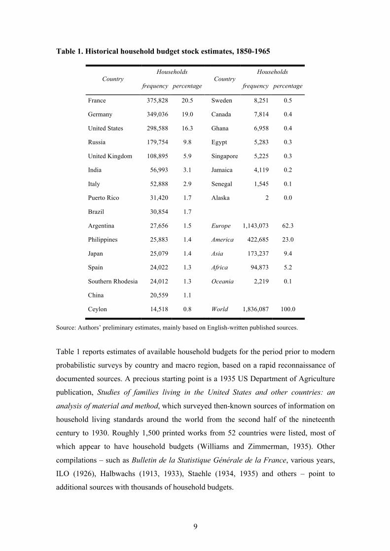
Table 1. Historical household budget stock estimates, 1850-1965

Country Households

Country Households

frequency percentage frequency percentage

France 375,828 20.5 Sweden 8,251 0.5

Germany 349,036 19.0 Canada 7,814 0.4

United States 298,588 16.3 Ghana 6,958 0.4

Russia 179,754 9.8 Egypt 5,283 0.3

United Kingdom 108,895 5.9 Singapore 5,225 0.3

India 56,993 3.1 Jamaica 4,119 0.2

Italy 52,888 2.9 Senegal 1,545 0.1

Puerto Rico 31,420 1.7 Alaska 2 0.0

Brazil 30,854 1.7

Argentina 27,656 1.5 Europe 1,143,073 62.3

Philippines 25,883 1.4 America 422,685 23.0

Japan 25,079 1.4 Asia 173,237 9.4

Spain 24,022 1.3 Africa 94,873 5.2

Southern Rhodesia 24,012 1.3 Oceania 2,219 0.1

China 20,559 1.1

Ceylon 14,518 0.8 World 1,836,087 100.0

Source: Authors’ preliminary estimates, mainly based on English-written published sources.

Table 1 reports estimates of available household budgets for the period prior to modern

probabilistic surveys by country and macro region, based on a rapid reconnaissance of

documented sources. A precious starting point is a 1935 US Department of Agriculture

publication, Studies of families living in the United States and other countries: an

analysis of material and method, which surveyed then-known sources of information on

household living standards around the world from the second half of the nineteenth

century to 1930. Roughly 1,500 printed works from 52 countries were listed, most of

which appear to have household budgets (Williams and Zimmerman, 1935). Other

compilations – such as Bulletin de la Statistique Générale de la France, various years,

ILO (1926), Halbwachs (1913, 1933), Staehle (1934, 1935) and others – point to

additional sources with thousands of household budgets.

10

Two comments on the figures in Table 1 are in order. First, the geographical

distribution is highly unbalanced (three countries account for more than 50% of total

observations; two thirds of all observations are for European countries). This is a

consequence of our preliminary research strategy rather than the likely availability of

actual data. Our research of has focused on countries for which the language barrier is

not an obstacle, which implies that Arabic, Chinese, some Slavic, and many South

Asian sources have not been even approached. This leads to the second remark, which is

that Table 1 is likely to show only the tip of the iceberg: for most countries we expect

that historical sources written in local languages outnumber sources in English and

other languages in which our compilations authors were proficient. In the case of Italy,

a back-of-the-envelope calculation suggests that the multiplier exceeds one hundred: for

each budget known to authors of the compilations, more than 100 where found in Italian

libraries, archives and secondary sources. The upshot of Table 1 is that huge numbers of

historical household budgets are available around the world.

Despite the relative abundance of source material, historical studies of household were

relatively few until relatively recently. But that is changing. Sara Horrell, Jane

Humphries and Deborah Oxley have pushed the approach well back in time, and also

pushed the limits of what we can learn.9 Following in their footsteps, other scholars

have used historical household budgets to study a range of themes. These include diet

and nutrition (Vecchi and Coppola, 2006; Logan, 2006, 2009; Gazeley and Horrell,

2013; Gazeley and Newell, 2015; Lundh, 2013), inequality and poverty (Rossi et al.

2001, Amendola and Vecchi, 2016), intra-household dynamics (Horrell and Oxley,

2013; Saaritsa and Kaihovaara, 2016; Scott, Walker and Miskell, 2015; Guyer, 1980),

labor force participation (Baines and Johnson, 1999), child labor (Moehling, 2001,

2005), consumption behavior (Scott and Walker, 2012; Lilja and Bäcklund, 2013),

agriculture and home-production (Federico, 1986, 1991), economies of scale and child

well-being (Hatton and Martin, 2010; Logan, 2011), and informal transfers of cash and

goods between households (Saaritsa, 2008, 2011).

Overall, the potential of household budgets for economic history has been exploited to

only a limited extent. Why? Because household budgets, as found in historical sources,

are very different from modern household budgets and historical household budgets

9 See, for example, Horrell and Humphries (1992; 1995; 1997), and Horrell and Oxley (1999; 2000).

11

cannot be treated as if they were modern household budgets: a collection of household

budgets, however large it may be, is not a representative sample and cannot

unproblematically be used for statistical inference about living conditions in the

population. Nor are historical data harmonized; the heterogeneity of the sources makes

the budgets too diverse to allow for consistent comparisons (Lanjouw and Lanjouw,

2001). Awareness of these limitations helps explain why economic historians have been

reluctant to use household budgets for the pre-statistical era. They believed, in short,

that household budgets were too scarce and sparse, too problematic and unreliable to

permit generalizations and to address big questions. Skepticism prevailed.

In the remainder of this article we narrow our focus to a specific theme among the many

that household budgets can illuminate – the long run evolution and distribution of living

standards. This is a field where a number of prominent figures have concentrated their

efforts (Steckel and Floud, 1997; Fogel, 2004; Allen et al. 2005, van Zanden et al. 2014;

Gordon, 2016). We illustrate the potential contribution of historical household budgets,

and present arguments that ought to win over the skeptics.

4 Inequality and poverty in the long run: the state of the art

While modern analysts can rely on household budget surveys, the perceived lack of

suitable data has been a major obstacle for economic historians. Several lines of inquiry

have emerged, even if we restrict our attention to monetary indicators and set to one

side approaches such as anthropometric history. We distinguish three schools and dub

them the Eclectics, the Heroics, and the Fiscalists10.

The Eclectics have discovered ingenious sources and methods (e.g., Soltow, 1968;

Williamson and Lindert, 1980; Williamson, 1985; Lindert, 2000). A common

denominator is the use of proxies for living standards, such as occupational pay ratios,

the window tax collected under the Inhabited House Duty in Britain, and probate

records (van Zanden et al. 2014). Reactions have not always been enthusiastic

(Feinstein, 1988). Moreover, the distance from the benchmark, the methods one would

employ with modern household budget surveys, is ample: proxy variables perform 10 While the names Eclectics and Fiscalists are self-describing, Heroics perhaps deserve an explanation. The idea is to evoke antiquity, about which some in the school have written, and the spirit of enterprise in calculating inequality in a remote period from rather sketchy data.

12

poorly in terms of both population coverage and theoretical consistency of the welfare

indicator.

That said, it is difficult to overstate the importance and influence of this first generation

of studies. They can be thought of as the second pillar of a bridge taking us from a lack

of interest in and knowledge about the historical distribution of income to an

empirically-grounded understanding of the long-run dynamics of inequality. The first

pillar is represented by Kuznets’s (1955) classic. As Kuznets tried to squeeze the most

out of his scant data, so did Lindert, Williamson and other scholars with their eclectic

conjectures.11 They succeeded in writing highly innovative pages of economic history,

opening up a new research field that is still flourishing today. Lindert and Williamson’s

(2016) latest book is the best evidence in support of the well-deserved fame of this

school.

The Heroics have explored the use of “social tables” for the pre-industrial era:

tabulations by contemporaries of average family incomes in different social strata

alongside population shares of these groups. The allure of social tables is hard to resist,

because they allow the analyst to roam widely in the past, from the Roman Empire in

the year 14 (Scheidel and Friesen, 2009) or Byzantium in year 1000, to Moghul India in

1750 or the Kingdom of Naples in 1811 (Milanovic, Lindert and Willamson, 2011;

Milanovic, 2011). On the basis of social tables van Zanden (1999) has estimated

inequality in European cities from 1500s onward, Hoffman et al. (2002) in European

countries since 1500, and Lindert and Williamson (2012) in the US over its first century

(1774-1860).

In parallel with the rediscovery of social tables, more refined statistical techniques have

been developed to analyze them. The tables report mean incomes only, offering no

information on within-group variation. Modalsli (2015) has recently suggested a

procedure for taking this into account when calculating inequality. Other efforts have

been directed at identifying the best choice for modeling income distributions, that is, of

interpolating income distributions.12 Interpolation, far from being an old-fashioned

topic, is highly relevant to historical studies (Atkinson, 2007: 39). Already a lengthy

menu of functional forms has been considered, including the lognormal, gamma, Pareto, 11 Lindert (2000: 174) writes that “(f)or Britain before 1914, our best guesses are necessarily eclectic. There is little choice but to weave an archival quilt of indirect clues on income inequality.” 12 ‘Best’ here mainly denotes superior empirical goodness-of-fit.

13

Weibull, Dagum, Singh-Maddala, Beta and Generalized Beta of the second kind

distributions (Jenkins, 2009). New studies continue to expand this list, increasing the

robustness and credibility of social table–based estimates (Hajargasht and Griffiths,

2013; Chotikapanich et al. 2013).

The Fiscalists, the school of Piketty and collaborators, rely on tax records. Adopting the

pioneering methods of Kuznets (1953) and Atkinson and Harrison (1978), the fiscalists

have succeeded in computing the shares of top incomes in the total, often on a yearly

basis, for a number of countries. Common methodological features of the fiscal

approach are the use of i) income tax data, ii) national accounts, and iii) Pareto

interpolation (that is, the assumption that the unobserved incomes below those at the top

follow a Pareto distribution). The relative abundance of ingredients i) and ii) combined

with the relentless activity of the school’s economists is the source of the recognition it

has received.

Results have been rich and have stimulated an intense debate both within academia and

among the public. An impressive two-volume work edited by Atkinson and Piketty

(2007, 2010), as well as a host of other publications – too many to be catalogued here –

have produced a large volume of data (Alvaredo et al., 2013). Since 2011 the World

Top Incomes Database (WTID) has made many findings publicly available for

download. Among the important results generated thus far is the empirical validation of

the Kuznets’s curve.

The work of the three schools is inspiring. But there remains room for improvement.

None of the sources used by the Eclectics meets the standard of modern analysis,

neither conceptually (the proxies for living standards do not have the properties

desirable for a comprehensive welfare indicator – see Deaton and Zaidi, 2002) nor

empirically (the sources employed being extremely heterogeneous). Nor do these

sources allow the analysts to tackle the multidimensional nature of living standards.

True, a number of difficulties have been overcome by the Fiscalists, but many

limitations remain. First, most top income share series start around the time of the First

World War, so time coverage is limited. Second, inequality measures based on tax

records are silent about what happens to the bottom 90% of the population, or even the

bottom 99%. This is a most serious limitation – modern analysts would despair in the

absence of 90-99% of the target population, and would mount a critique without mercy.

14

The nature of the problem is not too different from what occurs in modern surveys,

when investigators are faced with low response rates. There are remedies for dealing

with nonresponse, but they are effective only up to a point: beyond a certain threshold,

the entire survey becomes worthless (Lohr, 2009: ch. 8). Third, by failing to reconstruct

the entire income distribution, the WTID does not allow us to estimate the long-run

trend in poverty. This is worth emphasizing given the intellectual interest in the extent

to which economic growth is inclusive, and more specifically pro-poor. Fourth, WTID

considers only the income dimension of welfare and does not allow for multi-

dimensional poverty or inequality measures (Bourguignon and Chakravarty, 2003,

Alkire and Foster, 2011; Aaberge and Brandolini, 2014).

The limitations above discussed are of major concern to analysts interested in the long-

run evolution of living standards. A fourth school – still in search of a name – has been

founded on the idea of sending a modern welfare analyst back in time. Taking

advantage of i) knowledge and expertise in dealing with modern household budget data

and ii) the abundance of historical household budgets documented in Section 3, the

modern analyst working in the past would not seek new or more ingenious proxies for

living standards, but would construct a family budget based welfare indicator following

the best current practice. In so doing she would have a good chance of approaching the

“first best” solution discussed in Section 2. If anything like this were possible, it would

be a real advance in our understanding. Few economic historians have taken this path so

far, but interest is growing. Can we not send the welfare analyst back in time?

5 Working with historical household budgets – a user guide

Given the potential of historical household budgets, we need to discuss the ways they

differ from their modern counterparts. The key problems for which we need solutions

are those discussed in Section 2, namely i) non-representativeness (a historical

collection is not a statistical sample), and ii) non-standardization (historical sources vary

widely across many dimensions). Both issues pose serious conceptual and technical

problems; in this section we discuss how the time-traveling welfare analyst can handle

them, applying lessons learned by development economists immersed in a daily struggle

with troublesome data.

15

Non-representativeness. The lack of an underlying probabilistic survey design means

that no collection of historical budgets, no matter how large, can be assumed be a

statistical sample representative of the population. Some strata will be under-

represented, others unrepresented altogether in the data. Post-stratification

(stratification after collection of the sample) offers a viable solution to this problem

(Cochran, 1977: Ch. 5A; Holt and Smith, 1979). The idea is simple: we weight the

budgets in our historical collection so as to make its composition resemble the

population. Where to obtain appropriate weights? We can derive them from a

population census in a year close to that of our budgets. The census gives the

frequencies of different types of households: by region, by family composition and

ages, by occupation of the head of household, and so on. These frequencies are the

weights or “expansion factors” to be applied to the corresponding budgets in our

historical collection. The weighted budget collection can then be treated as if it were a

probabilistic sample.

Post-stratification is widely used in statistics, but is not a guarantee of success (Lohr,

2009: 114). A necessary condition is that the initial collection of budgets be sufficiently

numerous and representative of the target population. To clarify, with a collection of

only urban households there is no redemption, no way to magically produce nationally

representative estimates without some coverage of the rural sector.13 Assuming the data

are not affected by major problems of “non-coverage”, the question becomes: how

reliable is post-stratification, when applied to historical household budgets? The

evidence for Italy is that post-stratified statistics based on historical budget collections

agree closely with statistics based on the national accounts such as GDP per capita,

which is a non trivial result (Ravallion, 2001; Deaton, 2005).

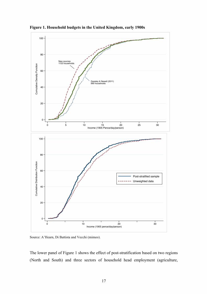
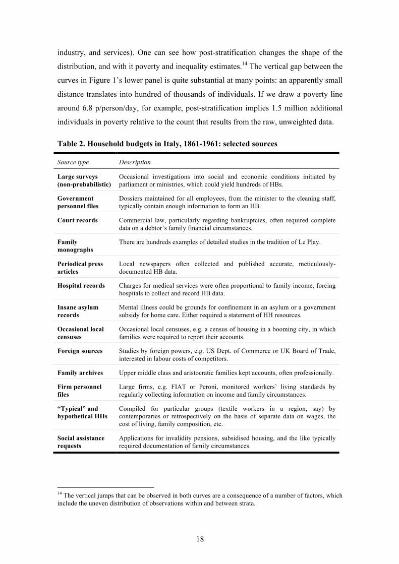
Figure 1 illustrates these issues in the case of the United Kingdom in the early 1900s.

The top panel shows the consequences of non-coverage; it plots the empirical

cumulative distributions of household income per capita in two samples. The Board of

Trade (BoT) sample comprises urban households only; the supplemental sample

includes both urban and rural households. It is immediately apparent that the BoT

13 “Non-coverage” – the complete omission from the sampling mechanism of some segments of the population, for instance rural households in a particular region, forces the researcher to turn to external, non-sample sources of information. Little and Rubin (2002) review a number of statistical techniques available to deal with non-coverage.

16

distribution lies everywhere to the right of (or below) the supplemental sample. If we

take any level of household income, a smaller share of the BoT households are below it,

a larger share above, compared with the supplemental sample. In technical terms, the

BoT sample distribution first-order stochastically dominates the new sample

(Atkinson, 1987). This first order stochastic dominance means that any poverty line

adopted will yield a smaller incidence of poverty – additional evidence beyond what we

know from documentary evidence that the BoT sample was not (intended to be)

representative of the entire population.

The effect of combining different sources, even if these originate entirely independently

and not as part of any coordinated survey process, is to mitigate the bias of any single

sample, and the inclusion of rural households clearly represents an improvement here.

But this is not sufficient to make the collection representative of the population of

Edwardian Britain. A second problem is caused by the unbalanced distribution of the

observations between rural and urban, or, within these categories, between regions or

sectors of activity. This is where post-stratification fits in.

17

Figure 1. Household budgets in the United Kingdom, early 1900s

Source: A’Hearn, Di Battista and Vecchi (mimeo).

The lower panel of Figure 1 shows the effect of post-stratification based on two regions

(North and South) and three sectors of household head employment (agriculture,

Gazeley & Newell (2011)990 households

New sources1153 households

0

20

40

60

80

100C

umul

ativ

e D

ensi

ty F

unct

ion

0 5 10 15 20 25 30Income (1905 Pence/day/person)

0

20

40

60

80

100

Cum

ulat

ive

Dis

tribu

tion

Func

tion

0 10 20 30Income (1905 pence/day/person)

Post-stratified sampleUnweighted data

18

industry, and services). One can see how post-stratification changes the shape of the

distribution, and with it poverty and inequality estimates.14 The vertical gap between the

curves in Figure 1’s lower panel is quite substantial at many points: an apparently small

distance translates into hundred of thousands of individuals. If we draw a poverty line

around 6.8 p/person/day, for example, post-stratification implies 1.5 million additional

individuals in poverty relative to the count that results from the raw, unweighted data.

Table 2. Household budgets in Italy, 1861-1961: selected sources

Source type Description

Large surveys (non-probabilistic)

Occasional investigations into social and economic conditions initiated by parliament or ministries, which could yield hundreds of HBs.

Government personnel files

Dossiers maintained for all employees, from the minister to the cleaning staff, typically contain enough information to form an HB.

Court records Commercial law, particularly regarding bankruptcies, often required complete data on a debtor’s family financial circumstances.

Family monographs

There are hundreds examples of detailed studies in the tradition of Le Play.

Periodical press articles

Local newspapers often collected and published accurate, meticulously-documented HB data.

Hospital records Charges for medical services were often proportional to family income, forcing hospitals to collect and record HB data.

Insane asylum records

Mental illness could be grounds for confinement in an asylum or a government subsidy for home care. Either required a statement of HH resources.

Occasional local censuses

Occasional local censuses, e.g. a census of housing in a booming city, in which families were required to report their accounts.

Foreign sources Studies by foreign powers, e.g. US Dept. of Commerce or UK Board of Trade, interested in labour costs of competitors.

Family archives Upper middle class and aristocratic families kept accounts, often professionally.

Firm personnel files

Large firms, e.g. FIAT or Peroni, monitored workers’ living standards by regularly collecting information on income and family circumstances.

“Typical” and hypothetical HHs

Compiled for particular groups (textile workers in a region, say) by contemporaries or retrospectively on the basis of separate data on wages, the cost of living, family composition, etc.

Social assistance requests

Applications for invalidity pensions, subsidised housing, and the like typically required documentation of family circumstances.

14 The vertical jumps that can be observed in both curves are a consequence of a number of factors, which include the uneven distribution of observations within and between strata.

19

Harmonization. The harvesting of historical household budgets implies recourse to

heterogeneous sources. In the case of Italy, Somogyi (1973) called household budgets a

“kaleidoscopic mosaic,” suggesting intricate detail and changing perspectives. But the

metaphor also reminds us of the fragmented and varied nature of the data. In historical

budget inquiries varying and imperfect coverage was the rule, not the exception. Sample

sizes varied from just one (!) – in the cases of some family monographs or “typical”

family budgets compiled by informed contemporaries – to a thousand and more.15 Table

2 illustrates the range of sources discovered and exploited thus far for Italy.

Constructing a standardized dataset is not a simple undertaking. Practically, it implies

that each record must be processed to conform to a uniform scheme (Browning, et al.,

2003) but historical sources vary widely: they have different reference periods (from a

single day up to an entire year), employ different methods of capturing data (diary vs.

recall), and report information with different levels of detail (at one extreme many

sources provide only total household income; at the other are sources with 50 and more

categories of expenditure). All this variety implies that the data – as reported in the

original sources – are not comparable (Beegle et. al 2014).

Two further issues are worth mentioning here. The first concerns grouped data.

Precious information, typically from mid-twentieth century sources, is frequently

presented in the form of histograms, or grouped data: separate tabulations giving the

number of households in different income categories, in different expenditure

categories, in different regions of residence, occupations or sectors of activity of the

household head, etc. Such empirical distributions allow us to calculate some measures

of interest directly, e.g. mean income, but they do not allow us to calculate, say, the

share of rural farming families that fall below a poverty line. Fortunately, new

techniques are being developed that aim to extract synthetic household-level data from

such tabulations (Shorrocks and Wan, 2008), and ongoing research in the area promises

further improvements in our ability to exploit historical data on household budgets. The

second issue relates to purchasing power parity exchange rates.

15 The most famous example is probably Frédéric Le Play’s (1806-1882) family monographs. See Lorry (2000).

20

5.1 Purchasing power parity (PPP) exchange rates.

Market exchange rates are the obvious candidate for converting local currency measures

to a common basis for comparison. Obvious, perhaps, but not obviously correct, since

market rates do not always reflect the actual purchasing power of currencies.

Economists today rely on PPP exchange rates, but reliable PPP standards, alas, are not

available for the period before 1950 (Deaton, 2010; Deaton and Heston, 2010).

A useful starting point for the discussion is to set out the issues algebraically. We begin

with household expenditure on goods and services. Let us denote by !!! the total

expenditure of household h in country j:

(1) !!! = !!,!!!!

!!!

In Eq. (1) !!,!! is household expenditure on a single good g, and the summation notation

indicates that we add up expenditures on all items in the set G. Typically, different

countries have different consumption habits, hence different, country-specific bundles

of goods and services, !!. These consumption baskets varied enormously across

countries and over time: imagine Ghana in 1850 and Sweden today. The relevance of

this point should not be underestimated; if the consumption bundles of two countries

show little or no overlap, the basis for meaningful cost-of-living comparisons between

countries becomes difficult, if not impossible.

Suppose we wish to compare expenditure across two households, say h and h’, in two

countries, say i and j. Each of !!! and !!!" is expressed in the relevant local currency.

The simplest conversion uses the market exchange rate !"!,! between the two

currencies:

!"!! =!!!!"!,!

; !"!!" =!!!"!"!,!

where !"!! and !"!!" are the expenditures of the two households expressed in a

common currency, the numeraire. In this case, country i’s currency is the numeraire and

!"!,! is the price of currency i in terms of currency j. If the dollar is the numeraire, !"!,! has units like £0.7/$ and !"!,! is $1/$. Thus !"!!" = !!!".

21

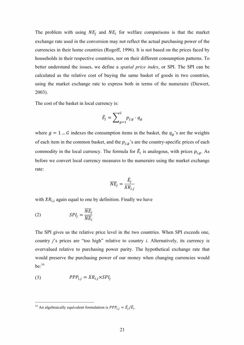
The problem with using !"! and !"! for welfare comparisons is that the market

exchange rate used in the conversion may not reflect the actual purchasing power of the

currencies in their home countries (Rogoff, 1996). It is not based on the prices faced by

households in their respective countries, nor on their different consumption patterns. To

better understand the issues, we define a spatial price index, or SPI. The SPI can be

calculated as the relative cost of buying the same basket of goods in two countries,

using the market exchange rate to express both in terms of the numeraire (Diewert,

2003).

The cost of the basket in local currency is:

!! = !!,! ⋅ !!!

!!!

where ! = 1…! indexes the consumption items in the basket, the !!’s are the weights

of each item in the common basket, and the !!,!’s are the country-specific prices of each

commodity in the local currency. The formula for !! is analogous, with prices !!,!. As

before we convert local currency measures to the numeraire using the market exchange

rate:

!"! =!!!"!,!

with !"!,! again equal to one by definition. Finally we have

(2) !"#! =!"!!"!

The SPI gives us the relative price level in the two countries. When SPI exceeds one,

country j’s prices are “too high” relative to country i. Alternatively, its currency is

overvalued relative to purchasing power parity. The hypothetical exchange rate that

would preserve the purchasing power of our money when changing currencies would

be:16

(3) !!!!,! = !"!,!×!"#!

16 An algebraically equivalent formulation is !!!!,! = !!/!!.

22

We can use this PPP standard to convert the local nominal expenditures of our two

households to real expenditures expressed in terms of the numeraire.

(4) !"!! =!"!!!!!!,!

(5) !"!!" =!"!!"!!!!,!

= !!!"

PPP estimation thus requires two ingredients, namely market exchange rates and spatial

price indices (Deaton and Muellbauer, 1980: Ch. 7; World Bank, 2013). The former

ingredient is not problematic: economic historians have been studying market exchange

rates for a long time. Regarding the SPI, its estimation in a historical context is more

complex.

Construction of an SPI requires i) a set of homogeneous consumption goods and

services (g=1…G) common to country i and country j; ii) market prices !!,! and !!,! of

these goods and services, and iii) the corresponding expenditure budget shares !! used

to weight items in the basket. In historical settings, information about prices is

fragmentary, often restricted to a few tradable goods (Allen, 2001). But for this subset

of goods, precisely because they are tradable, the law of one price is likely to hold, in

other words !!,! = !"!,!!!,! (otherwise there would be arbitrage opportunities,

abstracting from transaction costs). It is non-tradable goods – and services – that

motivate our interest in PPP in the first place. Even more difficult is the reconstruction,

with the required detail, of the average consumption pattern of the households. In

practice, measurement errors in i)-iii) can be large. In the absence of high quality

ingredients, a reasonable and defensible alternative may be to stick to the simpler recipe

of market exchange rates, using directly !"!! as a welfare indicator for international

comparisons. We will return to this in Section 7, when comparing Italy with the United

Kingdom in the early 1900s.

23

6 The Historical Household Budget (HHB) Project

The notion of combining tools from welfare economics and statistics with historical

(and modern) household budgets is more than just an idea. The authors of this paper

have launched an ambitious project – the Historical Household Budgets (HHB) Project

– to promote research into the evolution of living standards, within and between

countries, over the last two to three centuries.17 The project is interdisciplinary, long-

term, and unique in the way it has been envisaged.18 Here we offer a brief description.

HHB is based on a collaborative, open-source vision of research, and aims to provide a

publicly-available set of tools for working with household budgets that brings together

interested scholars from around the world. The Project is currently developing a web-

based infrastructure to host an HHB database. Given the abundance of data documented

earlier, and our ongoing bibliographic search for additional sources, we predict that the

database will eventually include several million household-level records, as well as

several terabytes of digital reproductions of source documents. But the database is about

more than just storage; the HHB web platform will allow researchers to enter, query,

and analyse household budget data in such as way as to permit seamless links between

countries and over time. Harmonisation is what this system aims at.

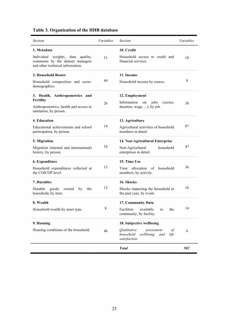
The HHB database (Table 3) comprises ca. 500 variables including monetary measures

of the standard of living (consumption, income, wealth, but also wages and retail

prices), education and health, anthropometric measures, fertility, employment and

migration, housing, agriculture, access to credit, and exposure to shocks.19 The design is

based on the World Bank’s Living Standard Measurement Study (Grosh and Glewwe,

2000) and the Luxembourg Income Study’s efforts to harmonize micro-datasets from

17 In fact, the period covered by the project covers household budgets that extend back to the 15th century – see Section 7. Sources for that era are sporadic and, presumably, rare. 18 Following Berry, Bourguignon and Morrison (1983), and Bourguignon and Morrison (2002), other projects have been developed, such as the University of Texas Inequality Project (http://utip.lbj.utexas.edu), and the “Global Consumption and Income Project” (http://gcip.info), described in Jayadev, Lahoti and Reddy (2015). These projects (as all other projects we are aware of) do not use historical microdata, that is household-level data before 1950, nor do they have a proper historical dimension. Much of their focus is instead on methodological issues. More importantly, none of the existing projects collects, harmonises and shares the microdata with users. None embraces the open-source vision that characterizes the HHB project. 19 Truth in advertising requires a disclaimer. The database has 500 variables to encompass the information reported across the full range of sources, but no individual source has so many items. Some sources in the database really are quite rich, though, e.g. Peruzzi’s monograph on a family of Tuscan sharecroppers in 1857. This study, conducted according to Le Play’s method, yields observations on 277 variables.

24

upper- and middle-income countries (Smeeding, Schmaus and Allegreza, 1985). Such

ex-post data harmonization is a task that ranks high on the agenda of many international

agencies, and HHB’s partnership links with LIS and the World Bank ensure that its

historical budgets will continue to be linkable with modern budgets.20

Given the tremendous variation across countries and over time, we need a scheme

flexible enough to accommodate diversity, a scheme both international and historical; at

the same time, we need this scheme to link to existing classifications. Variables must be

defined on a comparable basis, caloric content of food quantities must be calculated,

sometimes-archaic local units of measure must be automatically converted to a standard

reference, and so on. To cite but one of hundreds of examples, consider the staple

carbohydrate of many family diets, rice. There are many (more than 40,000!) varieties

of rice, which differ in price and nutritional content; we know that “rice” in New York

in 1895 is not the same as “rice” in Bombay in 1923. The HHB database goes beyond

the UN’s “COICOP” classification system, which does not distinguish rice by type, and

prompts the user to chose one of 44 basic types that can be identified from historical

sources.21

20 The construction of harmonized databases for exploring global trends in living standards is flourishing (Burkhauser and Lillard, 2005). In 2015, a special issue of the Journal of Income Inequality reviewed eight large-scale cross-national inequality databases – see Ferreira, Lustig and Teles (2015). 21 COICOP stands for Classification of Individual Consumption according to Purpose. Rice has the code 01.1.1 “rice in all forms”.

25

Table 3. Organization of the HHB database

Section Variables Section Variables

1. Metadata

Individual weights, data quality, comments by the dataset managers and other technical information.

51

10. Credit

Household access to credit and financial services.

18

2. Household Roster

Household composition and socio-demographics.

44 11. Income

Household income by source. 8

3. Health, Anthropometrics and Fertility

Anthropometrics, health and access to sanitation, by person.

26

12. Employment

Information on jobs (sector, duration, wage, ...), by job.

38

4. Education

Educational achievements and school participation, by person.

14 13. Agriculture

Agricultural activities of household members in detail.

87

5. Migration

Migration (internal and international) history, by person.

18 14. Non-Agricultural Enterprise

Non-Agricultural household enterprises in detail.

47

6. Expenditure

Household expenditures collected at the COICOP level.

13 15. Time Use

Time allocation of household members, by activity.

36

7. Durables

Durable goods owned by the household, by item.

12 16. Shocks

Shocks impacting the household in the past year, by event.

16

8. Wealth

Household wealth by asset type. 8 17. Community Data

Facilities available in the community, by facility.

14

9. Housing

Housing conditions of the household. 46

18. Subjective wellbeing

Qualitative assessment of household wellbeing and life satisfaction.

6

Total 502

26

7 On the job with the time-travelling welfare analyst

The approach described in earlier sections has been applied with some success, at least

in the Italian case. Here we give a flavour of the results generated by this research

programme, continuing to focus on the inter-household distribution of welfare. Linking

historic records of the sort set out in Table 2 with more recent survey data collected by

the Bank of Italy and the Italian Statistical Institute (Istat), Amendola and Vecchi

(2016) have produced estimates of the distribution of household income per capita that

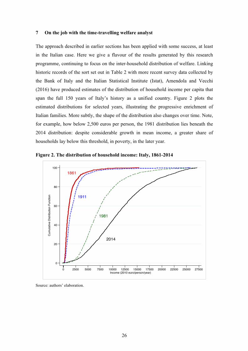
span the full 150 years of Italy’s history as a unified country. Figure 2 plots the

estimated distributions for selected years, illustrating the progressive enrichment of

Italian families. More subtly, the shape of the distribution also changes over time. Note,

for example, how below 2,500 euros per person, the 1981 distribution lies beneath the

2014 distribution: despite considerable growth in mean income, a greater share of

households lay below this threshold, in poverty, in the later year.

Figure 2. The distribution of household income: Italy, 1861-2014

Source: authors’ elaboration.

1861

1911

1981

2014

0

20

40

60

80

100

Cum

ulat

ive

Dis

tribu

tion

Func

tion

0 2500 5000 7500 10000 12500 15000 17500 20000 22500 25000 27500Income (2010 euro/person/year)

27

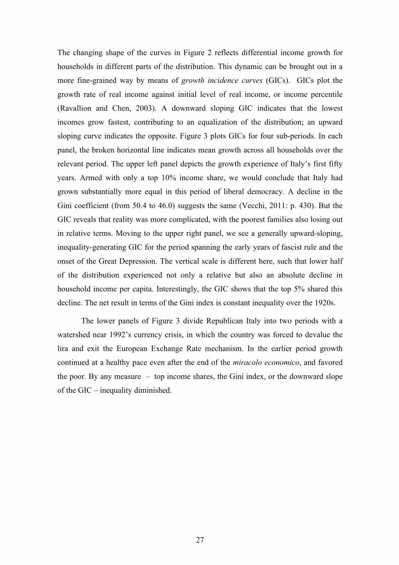
The changing shape of the curves in Figure 2 reflects differential income growth for

households in different parts of the distribution. This dynamic can be brought out in a

more fine-grained way by means of growth incidence curves (GICs). GICs plot the

growth rate of real income against initial level of real income, or income percentile

(Ravallion and Chen, 2003). A downward sloping GIC indicates that the lowest

incomes grow fastest, contributing to an equalization of the distribution; an upward

sloping curve indicates the opposite. Figure 3 plots GICs for four sub-periods. In each

panel, the broken horizontal line indicates mean growth across all households over the

relevant period. The upper left panel depicts the growth experience of Italy’s first fifty

years. Armed with only a top 10% income share, we would conclude that Italy had

grown substantially more equal in this period of liberal democracy. A decline in the

Gini coefficient (from 50.4 to 46.0) suggests the same (Vecchi, 2011: p. 430). But the

GIC reveals that reality was more complicated, with the poorest families also losing out

in relative terms. Moving to the upper right panel, we see a generally upward-sloping,

inequality-generating GIC for the period spanning the early years of fascist rule and the

onset of the Great Depression. The vertical scale is different here, such that lower half

of the distribution experienced not only a relative but also an absolute decline in

household income per capita. Interestingly, the GIC shows that the top 5% shared this

decline. The net result in terms of the Gini index is constant inequality over the 1920s.

The lower panels of Figure 3 divide Republican Italy into two periods with a

watershed near 1992’s currency crisis, in which the country was forced to devalue the

lira and exit the European Exchange Rate mechanism. In the earlier period growth

continued at a healthy pace even after the end of the miracolo economico, and favored

the poor. By any measure – top income shares, the Gini index, or the downward slope

of the GIC – inequality diminished.

28

Figure 3. Who benefited from economic growth?

Liberal Italy (1861-1911) Fascist Italy (1921-1931)

Modern Italy I (1977-1991) Modern Italy II (1991-2012)

Source: Amendola and Vecchi (2016).

In the quarter century since, this trend has been entirely reversed. The real incomes of

the poorest 30% have decreased in absolute terms; those of the next 60% (the middle

class) have stagnated; and only the richest 5-10% have seen significant growth.

The findings in Figures 3 and 4 are consolidated, robust results. We turn now to more

speculative comparative exercises that illustrate both the promise and some perils of our

approach. We first turn the time travelling welfare analyst’s dial all the way back to

1427, the year of a renowned tax survey (catasto) in Florence. The returns for all

households in the city survived, and constitute a precious source of data on family

wealth, size, and occupations. First subjected to computer analysis by Herlihy and

Klapisch-Zuber (1985), the catasto data have been revisited more recently by

0.2

0.4

0.6

0.8

1.0

Aver

age

year

ly g

row

th ra

te(%

)

0 10 20 30 40 50 60 70 80 90 100Percentiles of per capita income

-4.0

-2.0

0.0

2.0

4.0

Aver

age

year

ly g

row

th ra

te(%

)

0 10 20 30 40 50 60 70 80 90 100Percentiles of per capita income

1.0

2.0

3.0

4.0

5.0

Aver

age

year

ly g

row

th ra

te(%

)

0 10 20 30 40 50 60 70 80 90 100Percentiles of per capita income

-4.0

-2.0

0.0

2.0

Aver

age

year

ly g

row

th ra

te(%

)

0 10 20 30 40 50 60 70 80 90 100Percentiles of per capita income

29

Milanovic, Lindert, and Williamson (2011). Property income is directly available from

the catasto; the authors estimate labour income from the head of household’s

occupation and scattered observations on wage rates, combined with assumptions about

working days per year, the contributions of other family members, and the value of

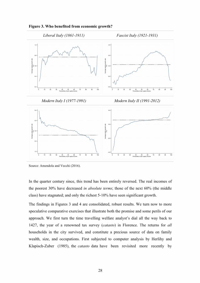
owner-occupied homes. Figure 4 illustrates the resulting distribution of family income

per capita, alongside the 1861 Italian distribution, reprised from Figure 2.

Figure 4. Four centuries and a half of decline

Source: authors’ elaboration on datasets kindly made available by Peter Lindert (Florence 1427)

and Amendola and Vecchi (Italy 1861).

The retrogression between 1427 and 1861 is dramatic; can this possibly be right? It does

correspond to the historiography of Italian economic decline, and to what we know

about real wages, urbanisation, and nutrition. Malanima’s (2011) estimates of North-

Italian GDP per capita in the long run indicate a 22% decline between 1427 and 1861.

But the contrast is exaggerated, for we are comparing the richest city of Renaissance

Italy’s richest region with all of Italy in 1861 including the poorest agricultural laborers

0

20

40

60

80

100

Cum

ulat

ive

Dis

tribu

tion

Func

tions

0 2000 4000 6000 8000 10000Income (2010 euro/person/year)

Florence 1427Italy 1861

30

of its poorest villages.22 The income estimates are also subject to wide margins of error.

Italian incomes of 1861 are directly observed, but for only a sample, while Florentine

incomes are only estimates, though available for every household in the city. The

conversion of 1427 florins to 2010 euros brings with it a further set of challenges.23

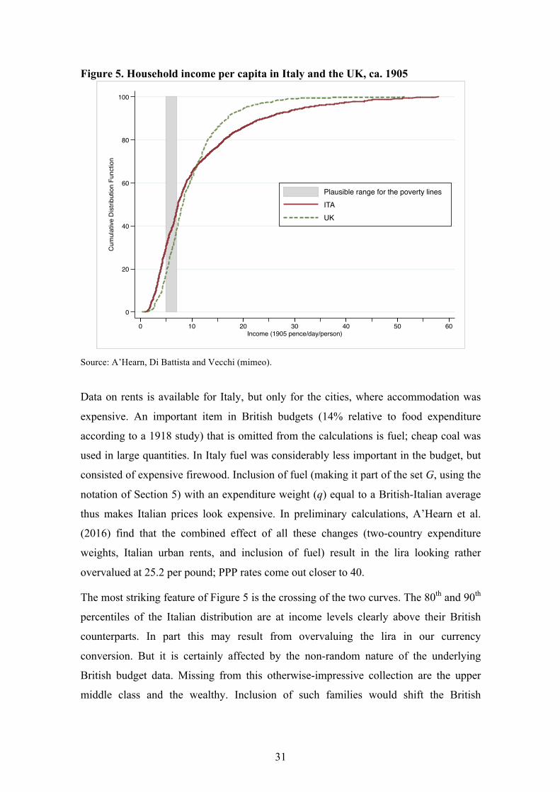
As interesting, and as difficult, as comparisons over time are those across countries.

Figure 5 illustrates a comparison of Italy and the UK in the first decade of the twentieth

century. The British data, already presented in Figure 1, are a large collection including

more than 900 households from the Board of Trade’s 1904 study of urban working

men’s families (Gazeley and Newell, 2011), the families of some 200 railway clerks

representing the lower middle class (Scott and Walker, 2015), and 920 family budgets

gleaned from 19 different studies covering a range of locations, sectors of employment,

and locations (A’Hearn, Di Battista, and Vecchi, 2016). The three-sector, two-region

post-stratification weighting is based on an interpolation of the 1901 and 1911

population censuses.

We express household incomes in 1905 domestic currency terms, using domestic price

indices, but then face the difficult task of picking a PPP exchange rate to convert Italian

lire to British pence. Williamson (1995) estimated this at 25.9 lire/pound, quite close to

the market exchange rate of 25.2 that is used in Figure 5. But Williamson’s calculation

can almost certainly be improved, for it is based almost entirely on 13 food items

common to the seven countries he compares. First, we should consider that dietary

patterns differed widely across these countries. Bread, for example, was 30% of Italian

food expenditure, just 14% of British, and 19% of the seven-country average used to

compute PPP standards. Or take butter: 13% of British, 2% of Italian, and 11% of

average expenditure. The only non-food item in the calculation is rent, which

unfortunately was not available for Italy and had to be imputed.

22 Lindert et al. estimate per capita income in the city at 153 Florentine lire. Malanima’s (2011) estimate for per capita GDP in all of North Italy is 63. This gives a sense of the relative wealth of the city of Florence. 23 For comparability we convert the 1427 figures from florins to euros of 2010 using Malanima’s (2011) North-Italian price index, additionally converting 1427 florins to 1427 Florentine lire at the rate of 4.15:1, Florentine lire to Italian lire at the 1861 rate of 3.8/4.5, and Italian lire to euros at the rate 1/1936.

31

Figure 5. Household income per capita in Italy and the UK, ca. 1905

Source: A’Hearn, Di Battista and Vecchi (mimeo).

Data on rents is available for Italy, but only for the cities, where accommodation was

expensive. An important item in British budgets (14% relative to food expenditure

according to a 1918 study) that is omitted from the calculations is fuel; cheap coal was

used in large quantities. In Italy fuel was considerably less important in the budget, but

consisted of expensive firewood. Inclusion of fuel (making it part of the set G, using the

notation of Section 5) with an expenditure weight (q) equal to a British-Italian average

thus makes Italian prices look expensive. In preliminary calculations, A’Hearn et al.

(2016) find that the combined effect of all these changes (two-country expenditure

weights, Italian urban rents, and inclusion of fuel) result in the lira looking rather

overvalued at 25.2 per pound; PPP rates come out closer to 40.

The most striking feature of Figure 5 is the crossing of the two curves. The 80th and 90th

percentiles of the Italian distribution are at income levels clearly above their British

counterparts. In part this may result from overvaluing the lira in our currency

conversion. But it is certainly affected by the non-random nature of the underlying

British budget data. Missing from this otherwise-impressive collection are the upper

middle class and the wealthy. Inclusion of such families would shift the British

0

20

40

60

80

100

Cum

ulat

ive

Dis

tribu

tion

Func

tion

0 10 20 30 40 50 60Income (1905 pence/day/person)

Plausible range for the poverty linesITAUK

32

distribution to the right. Still, we can make reliable comparisons of the lower tails.

Below about 10p per person per day, and particularly in the range of a plausible poverty

line, which would lie somewhat lower (in the shaded gray region), there are many more

Italian than British families. Observing the vertical distance between the distributions

we see that at least 10% more Italian families have daily per capita incomes of 5p or

less, relative to British. A higher rate of lire per pound or better coverage of well-off

families would shift the British distribution down or to the right, and could only

exacerbate this disparity.

The examples presented illustrate both the power and some of the perils of historical

household budget analysis. It has the potential to generate subtle insights into the

changing distribution of welfare across households, on a comparable basis, over long

periods of time, and across countries. At the same time it requires a clear-eyed

assessment of the limitations of the sources, depends to a considerable extent on non-

sample information such as price indices, and must be checked for corroboration against

alternative estimates.

8 Call to arms

We have argued three points about historical household budgets in these pages. First,

they represent the ideal type of data for addressing both micro questions about families

and macro questions about distribution. Second, they are far more numerous and

widespread than generally supposed. Third, the modern welfare analyst travelling back

in time already has a toolkit well-suited to dealing with the problems thrown up by

historical family data. All this leads us to conclude that historical household budgets, far

from a subject for antiquarians, have a bright future.

The challenges of this research agenda should not be underestimated. The technical

difficulties to which we have devoted most of our attention here – non-

representativeness, non-standardization, and currency conversions over long time

periods or across countries – are capable of solution, but only at the cost of painstaking

work with the sources, engagement with the relevant statistical techniques, and the

search for complementary information on population structure and the prices of

consumption items. But if the challenges are great, so too is the payoff. Should the HHB

33

Project’s aim of making the micro data and the welfare indicators derived from them

comparable over time and across countries be realised, we will be in a vastly better

position to understand the historical development of living standards, the distribution of

welfare, and how they responded to technical, institutional, and policy changes.

So we conclude with a call to arms. There is a need for every sort of contribution, from

the discovery of apparently insignificant budget sources to the perfection of minor

variations on a technique for estimating distributions to the development of new

historical narratives and interpretive frameworks. Lend your talents and energies to the

fight.

34

References

A’Hearn, B., F. Di Battista and G. Vecchi (2016), “Old questions, old data, and a new approach: Poverty in the United Kingdom at the rise of the 20th century”, mimeo.

Aaberge, R., and A. Brandolini (2014), ‘Multidimensional Poverty and Inequality’. In A.B. Atkinson and F. Bourguignon (eds.), Handbook of Income Distribution, vol. 2A, ch. 4. Elsevier.

Alkire, S., and J. Foster (2011), ‘Counting and multidimensional poverty measurement’, Journal of Public Economics, 95(7): 476-487.

Allen, R. (2001), ‘The Great Divergence in European Wages and Prices from the Middle Ages to the First World War’, Explorations in Economic History, 38: 411-47.

Allen, R., J.P. Bassino, D. Ma, C. Moll-Murata, and J.L. van Zanden, (2005), ‘Wages, prices and living standards in China, Japan and Europe’, The Economic History Review, 64(S1) 8-38.

Alvaredo, F., A.B. Atkinson, T. Piketty, and E. Saez (2013), ‘The top 1 percent in international and historical perspective’, NBER Working Paper 19075.

Amendola, N., and G. Vecchi (2016), ‘Inequality’, in G. Vecchi, Measuring Well-being. A history of Italian living standards, Ch. 8. Oxford University Press.

Amendola, N., G. Gabbuti, G., and G. Vecchi (2016), ‘Human Development’, in G. Vecchi, Measuring Well-being. A History of Italian Living Standards, Ch. 12. Oxford University Press.

Anand, S. and A. Sen (1994) ‘Human Development Index: Methodology and Measurement’, United Nation Development Report Office, Occasional Paper.

Atkinson, A. B. (1987), ‘On the measurement of poverty’, Econometrica, 55(4): 749-764.

Atkinson, A. B. (2007), ‘The distribution of top incomes in the United Kingdom 1908–2000.’, in Atkinson, A.B., and T. Piketty (eds.), Top Incomes over the Twentieth Century: A Contrast between Continental European and English-Speaking Countries, 1: 82-140. Oxford University Press.

Atkinson, A.B. (2015), Inequality. What can be done? Harvard University Press.

Atkinson, A.B., and A.J. Harrison (1978), Distribution of personal wealth in Britain. Cambridge University Press.

Atkinson, A. B., and T. Piketty (eds.), (2010), Top incomes: A global perspective. Oxford University Press

Atkinson, A. B., and T. Piketty (eds.), (2007), Top incomes over the twentieth century: a contrast between continental european and english-speaking countries. OUP

35

Oxford.

Baines, D., and P. Johnson (1999), ‘Did they jump or were they pushed? The exit of older men from the London labor market, 1929–1931’, The Journal of Economic History, 59(04): 949-971.

Bales, K., M. Bulmer, and K.K. Sklar, (1991), The Social Survey in Historical Perspective, 1880-1940. Cambridge University Press.

Beegle, K., J. De Weerdt, J. Friedman, and J. Gibson (2012), ‘Methods of household consumption measurement through surveys: Experimental results from Tanzania’, Journal of Development Economics, 98, 3–18.

Berry, A., F. Bourguignon, and C. Morrison (1983), ‘Changes in the world distribution of income between 1950 and 1977’, The Economic Journal, 93(370): 331-350.

Bourguignon, F. (2015), The Globalization of Inequality. Princeton University Press.

Bourguignon, F., and S.R. Chakravarty (2003), ‘The measurement of multidimensional poverty’, The Journal of Economic Inequality, 1(1): 25-49.

Bourguignon, F., and C. Morrisson (2002), ‘Inequality among world citizens: 1820-1992’, American Economic Review, 92(4): 727-744.

Browning, M. , T.F. Crossley, and G. Weber, (2003) ‘Asking consumption questions in general purpose surveys’, The Economic Journal, 113: F540-F567.

Burkhauser, R.V., N. Hérault, S.P. Jenkins, and R. Wilkins (2016), ‘What has been happening to UK income inequality since the mid-1990s? Answers from reconciled and combined household survey and tax return data’, NBER Working paper 21991.

Burkhauser, R.V., and D.R. Lillard (2005), ‘The contribution and potential of data harmonization for cross-national comparative research’, Journal of Comparative Policy Analysis, 7(4): 313-330.

Chianese, S., and G. Vecchi (2016), ‘Household budgets’, in G. Vecchi, Measuring Well-being. A history of Italian living standards. Ch. 13. Oxford University Press.

Chotikapanich, D., W. Griffiths, W. Karunarathne, and D.S. Prasada Rao (2013), ‘Calculating poverty measures from the generalised beta income distribution’, Economic Record, 89(S1): 48-66.

Cochran, W. (1977), Sampling techniques. New York, Wiley and Sons, 98, 259-261.

Converse, J.M. (1987), Survey Research in the United States: Roots and Emergence, 1890-1960. University of California Press.

Darrow, D. W. (2000), ‘The Politics of Numbers: Zemstvo Land Assessment and the Conceptualization of Russia's Rural Economy’. The Russian Review, 59(1), 52-75.

36

Davie, G. (2015), Poverty Knowledge in South Africa: A Social History of Human

Science, 1855-2005. Cambridge University Press.

Deaton, A. (2013), The Great Escape: Health, Wealth, and the Origins of Inequality. Princeton University Press.

Deaton, A. (1997), The Analysis of Household Surveys: A Microeconometric Approach to Development Policy. The World Bank.

Deaton, A. (2005), ‘Measuring poverty in a growing world (or measuring growth in a poor world)’, Review of Economics and statistics, 87(1): 1-19.

Deaton, A. (2010). “Price indexes, inequality, and the measurement of world poverty”, American Economic Review, 100: 1, 5–34.

Deaton, A., and Grosh, M. (1998), “Designing Household Survey Questionnaires for Developing Countries Lessons from Ten Years of LSMS Experience”, Chapter 17: Consumption (No. 218).

Deaton, A., and A. Heston (2010), ‘Understanding PPPs and PPP-based national accounts’. American Economic Journal: Macroeconomics, 2(4), 1–35.

Deaton, A., and J. Muellbauer (1980), Economics and Consumer Bbehavior. Cambridge University Press.

Deaton, A., and S. Zaidi (2002), ‘Guidelines for constructing consumption aggregates for welfare analysis’, World Bank LSMS working paper 135.

Dercon, S. (2004), Insurance Against Poverty. Oxford University Press.

Devarajan, S. (2013), ‘Africa's statistical tragedy’. Review of Income and Wealth, 59(S1), S9-S15.

Diewert, E. (2003), ‘Basic index number theory’, Chapter 15 in The Consumer Price Index Manual: Theory and Practice Geneva: International Labour Organization.

Eaton, A.H., and S.M. Harrison (1930), A bibliography of social surveys: reports of fact-finding studies made as a basis for social action. Russell Sage Foundation.

Fang, C., E. Wailes, and G. Cramer (1998), ‘China's rural and urban household survey data: Collection, availability, and problems’, CARD Working Papers, 247.

Federico, G. (1986), ‘Mercantilizzazione e sviluppo economico in Italia (1860-1940)’, Rivista di Storia Economica, n.s. III: 149-186.

Federico, G., (1991). ‘Household budgets as a source for the study of rural economy (Italy, 1860–1940): Commercialization and peasants behaviour., in Toni, P. (ed.), Zur Öekonomik des privaten Haushalts. Campus Verlag, 182–197.

Feinstein, C. (1988), ‘The rise and fall of the Williamson curve’, The Journal of

37

Economic History, 48(03): 699-729.

Ferreira, F.H., N. Lustig, and D. Teles (2015), ‘Appraising cross-national income inequality databases: An introduction’, The Journal of Economic Inequality, 13(4): 497-526.

Field, D. (1989), ‘The Polarization of Peasant Households in Prerevolutionary Russia: Zemstvo Censuses and Problems of Measurement’, Research in Economic History: 477-505.

Figari, F., A. Paulus, and H. Sutherland (2014), ‘Microsimulation and policy analysis’, ISER Working Paper Series, 2014-23.

Fleurbaey, M. (2009), ‘Beyond GDP: The quest for a measure of social welfare’. Journal of Economic Literature, 47(4): 1029-1075.

Fogel, R.W. (2004), The Escape from Hunger and Premature Death, 1700-2100: Europe, America, and the Third World. Cambridge University Press.

Gazeley, I., and S. Horrell (2013), ‘Nutrition in the English agricultural labourer's household over the course of the long nineteenth century’, The Economic History Review, 66(3), 757-784.

Gazeley, I., and A. Newell (2015), ‘Urban working-class food consumption and nutrition in Britain in 1904’, The Economic History Review, 68(1): 101-122.

Gazeley, I., and A. Newell (2011), ‘Poverty in Edwardian Britain’, The Economic History Review, 64(1): 52-71.

Gordon, R.J. (2016), The Rise and Fall of American Growth: The US Standard of Living since the Civil War. Princeton University Press.

Grosh, M., and P. Glewwe (2000), Designing Household Survey Questionnaires for Developing Countries. Lessons from 15 Years of the Living Standards Measurement Study. The World Bank.

Guyer, J. I. (1980), ‘Household budgets and women's incomes’. African Studies Center, Boston University. Working paper 28.

Hajargasht, G., and W.E. Griffiths, (2013), ‘Pareto–lognormal distributions: Inequality, poverty, and estimation from grouped income data’. Economic Modelling, 33: 593-604.

Halbwachs, M. (1913). La classe ouvrière et les niveaux de vie. Alcan.

Halbwachs, M. (1933). ‘Budgets de famille’. In Annales d'histoire économique et sociale, p. 184-186. Armand Colin.

Hatton, T.J., and R.M. Martin (2010), ‘Fertility decline and the heights of children in Britain, 1886–1938’, Explorations in Economic History, 47(4): 505-519.

38

Herlihy, D., and C. Klapisch-Zuber (1985), Tuscans and their families: a study of the Florentine catasto of 1427. Editions de l'Ecole des Hautes Etudes en Sciences Sociales Ouvrage, (8).

Hiroko, T. (2004), The Political Economy of Reproduction in Japan. Routledge.

Hoffman, P. T., D.S. Jacks, P.A. Levin, and P.H. Lindert (2002), ‘Real inequality in Europe since 1500’, The Journal of Economic History, 62(02): 322-355.

Holt, D., and Smith, T. M. F. (1979), ‘Post stratification’. Journal of the Royal Statistical Society. Series A (General), 33-46.

Horrell, S., and J. Humphries (1997), ‘The origins and expansion of the male breadwinner family: The case of nineteenth-century Britain’, International Review of Social History, 42(S5): 25-64.

Horrell, S., and J. Humphries (1995), ‘The Exploitation of Little Children: Child Labor and the Family Economy in the Industrial Revolution’, Explorations in Economic History, 32(4): 485-516.

Horrell, S., and J. Humphries (1992), ‘Old questions, new data, and alternative perspectives: families' living standards in the industrial revolution’, The Journal of Economic History, 52(04): 849-880.

Horrell, S., and D. Oxley (2013), ‘Bargaining for basics? Inferring decision making in nineteenth-century British households from expenditure, diet, stature, and death’, European Review of Economic History, 17(2): 147-170.

Horrell, S., and D. Oxley (2000), ‘Work and prudence: Household responses to income variation in nineteenth-century Britain’, European Review of Economic History, 4(1): 27-57.

Horrell, S., and D. Oxley (1999), ‘Crust or crumb?: Intrahousehold resource allocation and male breadwinning in late Victorian Britain’, The Economic History Review, 52(3): 494-522.

International Labour Office (1926), ‘Methods of conducting family budgets enquiries’, Studies and reports, Series N, no. 9.

International Labour Office (1949), ‘Methods of Family Living Studies’, Studies and reports, Series N, no. 17.

International Labour Office (1961), ‘Family Living Studies: A symposium’, Studies and reports, Series N, no. 63.

International Labour Office (2004), Consumer price index manual. Theory and practice, ILO.

Jäntti, M. (2006), ‘Income distribution in the 20th century’, in Ojala, J., J. Eloranta and J. Jalava (eds.), Road to Prosperity: An Economic History of Finland.

39

Suomalaisen Kirijallisuuden Seuran Toimituksia.

Jayadev, A., R. Lahoti, and S.G. Reddy (2015), ‘Who Got What, Then and Now? A Fifty Years Overview from the Global Consumption and Income Project’, Courant Research Centre PEG, 174.

Jenkins, S. P. (2009), ‘Distributionally-Sensitive Inequality Indices and The Gb2 Income Distribution’, Review of Income and Wealth, 55(2), 392-398.

Jerven, M. (2015), Measuring African Development: Past and Present. Routledge.

Komori, N. (2007), ‘The “hidden” history of accounting in Japan: a historical examination of the relationship between Japanese women and accounting’. Accounting History, 12(3), 329-358.

Kotz, S., and E. Seneta (1990), ‘Lenin as a statistician: a non-soviet view’. Journal of the Royal Statistical Society. Series A, 153(1): 73-94.

Kuznets, S. (1955), ‘Economic growth and income inequality’, The American Economic Review, 45(1), 1-28.

Kuznets, S. S. (1953), Shares of Upper Income Groups in Income and Savings. Cambridge, Mass.: National Bureau of Economic Research.

Lanjouw, J. O., and P. Lanjouw, P. (2001), ‘How to compare apples and oranges: poverty measurement based on different definitions of consumption’, Review of Income and Wealth, 47(1), 25-42.

Lequiller, F., D.W. Blades, and D. Blades (2006), Understanding National Accounts. OECD Publishing.

Levy, P.S., and S. Lemeshow (1999), Sampling of populations. Methods and applications. Wiley.

Lilja, K., and D. Bäcklund (2013), ‘To navigate the family economy over a lifetime: life-cycle squeezes in pre-industrial Swedish towns’, European Review of Economic History, 17(2): 171-189.

Lindert, P.H. (2000), ‘Three centuries of inequality in Britain and America’, in A.B. Atkinson and F. Bourguignon (eds.), Handbook of income distribution, 1, 167-216. Elsevier.

Lindert, P.H., and S. Nafziger (2012), ‘Russian inequality on the eve of revolution’, NBER Working paper 18383.

Lindert, P.H., and Williamson, J.G. (2016), Unequal Gains: American Growth and Inequality since 1700. Princeton University Press.

Lindert, P.H., and J.G. Williamson (2012), ‘American Incomes 1774-1860’, NBER Working Paper 18396.

40

Little, R.J., and D.B. Rubin (2014), Statistical analysis with missing data. John Wiley & Sons.

Logan, T.D. (2011), ‘Economies of scale in the household: Puzzles and patterns from the American past’. Economic Inquiry, 49(4), 1008-1028.

Logan, T.D. (2009), ‘The transformation of hunger: The demand for calories past and present’. The Journal of Economic History, 69(02): 388-408.

Logan, T.D. (2006), ‘Nutrition and Well-Being in the Late Nineteenth Century’. The Journal of Economic History, 66(02): 313-341.

Lohr, S. (2009), Sampling: design and analysis. Nelson Education.

López-Alonso, M. (2012), Measuring Up: A History of Living Standards in Mexico, 1850–1950. Stanford University Press.

Lorry, A. (2000), ‘Les monographies des Ouvriers européens (1855 et 1877-79) et des Ouvriers des deux mondes (1857-1930): inventaire et classification’, Les Études sociales, (131-132), 1: 93-181.

Lundh, C. (2013), ‘Was there an urban–rural consumption gap? The standard of living of workers in southern Sweden, 1914–1920’, Scandinavian Economic History Review, 61(3): 233-258.

Malanima, P. (2011), ‘The long decline of a leading economy: GDP in central and northern Italy, 1300–1913’, European Review of Economic History, 15(02): 169-219.

Marivoet, W., and T. De Herdt (2015), ‘Poverty lines as context deflators: a method to account for regional diversity with application to the Democratic Republic of Congo’, Review of Income and Wealth, 61(2), 329-352.

Meyer, B.D., W. Mok, and J.X. Sullivan (2015), ‘Household Surveys in Crisis’. NBER Working Paper 21399.

Milanovic, B. (2016), Global Inequality: A New Approach for the Age of Globalization. Harvard University Press.

Milanovic, B. (2011), Worlds Apart. Measuring international and global inequality. Princeton University Press.

Milanovic, B., P.H. Lindert, and J.G. Williamson, (2011), ‘Pre-Industrial Inequality’, The Economic Journal, 121(551): 255-272.

Modalsli, J. (2015), ‘Inequality in the very long run: inferring inequality from data on social groups’, The Journal of Economic Inequality, 13(2): 225-247.

Moehling, C. M. (2005), ‘She Has Suddenly Become Powerful: Youth Employment and Household Decision Making in the Early Twentieth Century’, The Journal of

41

Economic History, 65(02): 414-438.

Moehling, C.M. (2001), ‘Women's work and men's unemployment’, The Journal of Economic History, 61(4): 926-949.

O’Rourke, K. H., and J.G. Williamson, (1999), Globalization and History. The Evolution of a 19th Century Atlantic Economy. MIT Press.

Öberg, S. (forthcoming), ‘Did the poor pay more? Income-related variations in diet and food quality among urban households in Sweden, 1913–1914’, Rivista di Storia Economica, n. 2, 2016.

Ogura, E. (1982), ‘The Nakai family's bookkeeping system’, Accounting and Business Research, 12(46), 148-152.

Peragine, V. (2004), ‘Measuring and implementing equality of opportunity for income’. Social Choice and Welfare, 22(1), 187-210.

Piketty, T. (2014), Capital in the Twenty-First Century. Harvard University Press.

Ravallion, M. (2001), ‘Growth, inequality and poverty: looking beyond averages’, World development, 29(11): 1803-1815.

Ravallion, M., and S. Chen (2003), ‘Measuring pro-poor growth’, Economics Letters, 78(1): 93-99.

Rogoff, K. (1996), ‘The Purchasing Power Parity Puzzle’, Journal of Economic Literature, 34 (2): 647-668.

Roberts, E. (forthcoming), ‘Household budget studies in the British dominions, 1873-1939’, Rivista di Storia Economica, n. 2, 2016.

Rossi, N., G. Toniolo, and G. Vecchi (2001), ‘Is the Kutznets Curve Still Alive? Evidence from Italy’s Household Budgets, 1881-1961’, The Journal of Economic History, 61(4): 904-925.

Saaritsa, S. (forthcoming), ‘Data to Die For? Finnish Historical Household Budgets’, Rivista di Storia Economica, n. 2, 2016.

Saaritsa, S., and Kaihovaara, A. (2016), ‘Good for girls or bad for boys? Schooling, social inequality and intrahousehold allocation in early twentieth century Finland’, Cliometrica, 10(1): 55-98.

Saaritsa, S. (2011), ‘The poverty of solidarity: the size and structure of informal income smoothing among worker households in Helsinki, 1928’. Scandinavian Economic History Review, 59(2): 102-127.

Saaritsa, S. (2008), ‘Informal transfers, men, women and children: Family economy and informal social security in early 20th century Finnish households’, The History of the Family, 13(3): 315-331.

42

Scheidel, W., and Friesen, S. J. (2009), ‘The Size of the Economy and the Distribution of Income in the Roman Empire’, Journal of Roman Studies, 99: 61-91.

Scott, P., and J.T. Walker (2015), 'Demonstrating distinction at ‘the lowest edge of the black-coated class’: The family expenditures of Edwardian railway clerks’, Business History, 57(4) 564-588.

Scott, P.M., and J.T. Walker (2012), ‘Working-Class Household Consumption Smoothing in Interwar Britain’, The Journal of Economic History, 72(3): 797-825.

Scott, P., J.T. Walker, and P. Miskell (2015), ‘British working-class household composition, labour supply, and commercial leisure participation during the 1930s’, The Economic History Review, 68(2): 657-682.

Seneta, E. (1985), ‘A sketch of the history of survey sampling in Russia’, Journal of the Royal Statistical Society (Series A), 148(2): 118-125.

Serra, G. (2014), ‘An uneven statistical topography: the political economy of household budget surveys in late colonial Ghana, 1951–1957’, Canadian Journal of Development Studies, 35 (1): 9-27.

Shorrocks, A., and G. Wan (2008), ‘Ungrouping income distributions: Synthesising samples for inequality and poverty analysis’, UNU-WIDER Research Paper 2008/16.

Smeeding, T., G. Schmaus, and S. Allegreza (1985), ‘An introduction to LIS’. LIS-CEPS Working Paper, 1.

Smith, W. (1873). A Dictionary of Greek and Roman Antiquities. London: John Murray.

Smitka, M. (ed.), (1998), Historical demography and labor markets in prewar Japan, Vol. 3, Taylor & Francis.

Soltow, L. (1968), ‘Long-Run Changes in British Income Inequality’, The Economic History Review, 21(1): 17-29.

Somogyi, S. (1973), ‘L’alimentazione nell’Italia unita’. Storia d'Italia, vol. 5. Einaudi.

Staehle, H. (1934), ‘Annual Survey of Statistical Information: Family Budgets’, Econometrica, 2(4): 349-362.

Staehle, H. (1935). ‘Family Budgets’, Econometrica, 3(1): 106-118.

Stapleford, T.A. (2009), The Cost of Living in America: A Political History of Economic Statistics, 1880-2000. Cambridge University Press.

Steckel, R. H., and R. Floud (eds.) (1997), Health and Welfare during Industrialization. University of Chicago Press.

Stigler, G. J. (1954), ‘The early history of empirical studies of consumer behavior’. The

43

Journal of Political Economy, LXII, 95-113.

Thomas, R.L. (1987), Applied Demand Analysis. London and New York: Longman.

van Zanden, J.L. (1999), ‘Wages and the Standard of Living in Europe, 1500-1800’, European Review of Economic History, 3(2): 175-197.

van Zanden, J.L., J. Baten, M. Mira D’Ercole, A. Rijpma, C. Smith and M. Timmer (eds.) (2014), How Was Life?: Global Well-being since 1820, OECD Publishing, Paris.

van Zanden, J.L., J. Baten, P. Foldvari, and B. Leeuwen (2014), ‘The Changing Shape of Global Inequality 1820–2000; Exploring a New Dataset’. Review of Income and Wealth, 60(2): 279-297.

Vecchi, G. (2016), Measuring Well-being. A History of Italian Living Standards. Oxford University Press.

Vecchi, G. (2011), In ricchezza e in povertà. Il benessere degli italiani dall'Unità a oggi. Il Mulino.

Vecchi, G., and M. Coppola (2006), ‘Nutrition and growth in Italy, 1861–1911: What macroeconomic data hide’, Explorations in Economic History, 43(3); 438-464.

Williams, F.M., and C.C. Zimmerman (1935), Studies of family living in the United States and other countries: an analysis of material and method. United States Department of Agriculture, Miscellaneous Publications no. 323.

Williamson, J.G. (1985). Did British Capitalism Breed Inequality? Winchester: Allen & Unwin.

Williamson, J.G. (1995), ‘The evolution of global labor markets since 1830: background evidence and hypotheses’. Explorations in Economic History, 32(2), 141-196.

Williamson, J.G. and P.H. Lindert (1980). American Inequality: a Macroeconomic History, New York, Academic Press.

Woodbury, R.M. (1940), ‘Methods of family living studies. Income-expenditure-consumption’. International Labour Office Studies and Reports, Series N, no. 23.

World Bank (2013), The Framework, Methodology, and Results of the International Comparison Program—ICP. The World Bank.

UNIVERSITY OF OXFORD DISCUSSION PAPERS IN ECONOMIC AND SOCIAL HISTORY

are edited by

Rui Esteves (Brasenose College, Oxford, OX1 4AJ) Gabriel Geisler Mesevage (Brasenose College, Oxford, OX1 4AJ)

!

Papers!may!be!downloaded!from!!

http://www.economics.ox.ac.uk/index.php/working<papers/oxford<economic<and<social<history<working<papers!

!

!