WIS Geospatial identification of optimal straw-to-energy conversion sites in the Pacific Northwest
23
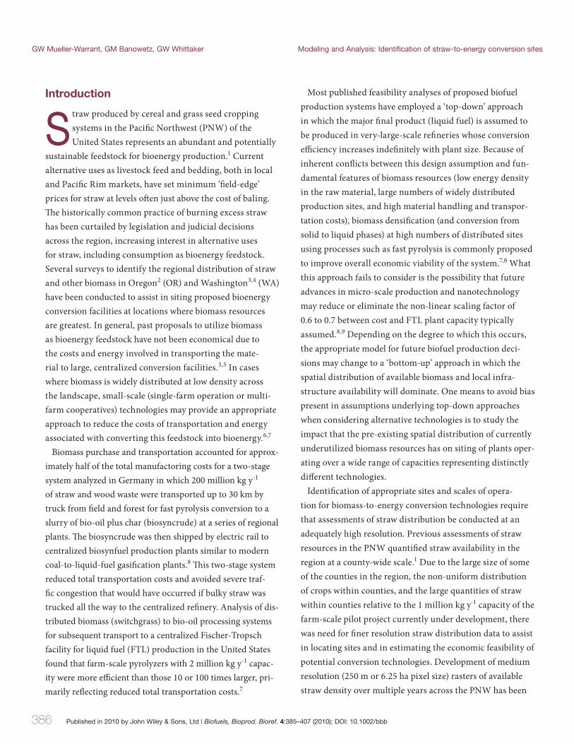
Published in 2010 by John Wiley & Sons, Ltd Correspondence to: George W. Mueller-Warrant, USDA-ARS, National Forage Seed Production Research Centre, 3450 SW Campus Way, Corvallis, OR 97331, USA. E-mail: [email protected]. † This article is a US Government work and is in the public domain in the USA. 385 Modeling and Analysis Geospatial identification of optimal straw-to-energy conversion sites in the Pacific Northwest † George W. Mueller-Warrant, Gary M. Banowetz and Gerald W. Whittaker, USDA-ARS, Corvallis, OR, USA Received November 5, 2009; revised March 19, 2010; accepted April 1, 2010 Published online in Wiley InterScience (www.interscience.wiley.com); DOI: 10.1002/bbb.230; Biofuels, Bioprod. Bioref. 4:385–407 (2010) Abstract: Previous attempts to develop straw-based bioenergy systems have stumbled at costs of transporting this low-density resource to large-scale, centralized facilities. Success in developing small-scale, distributed technolo- gies (e.g. syngas or pyrolysis bio-oil) that reduce these costs will depend on closely matching system requirements to spatial distribution of available straw. We analyzed straw distribution in the Pacific Northwest to identify optimal sites for facilities ranging from a pilot plant currently under development to larger ones of previous studies. Sites for plants with capacities of 1, 10, or 100 million kg straw y -1 were identified using a ‘lowest-hanging-fruit’ iterative siting process in which the location of maximum density of straw over an appropriately sized neighborhood was identified, distance from that point necessary to include desired quantity of straw measured, straw assigned to that plant removed from the raster, and the process repeated until all available straw had been assigned. Compared to K-means, our new method sited the first 44% of plants at superior locations in terms of local straw density (i.e. lower transportation costs) and the next 39% at equivalent locations. K-means produced better locations for the final 17% of plants along with superior average results. For the smallest facilities at locations defined by 3-year average availa- ble straw density, 1.2 km buffers were adequate to provide straw for the first 10% of plants, with twice that distance sufficient for the first 70%. For the largest plants, 12 km buffers satisfied the first 10% of plants, with 24 km buff- ers satisfying the first 60%. Buffer distances exceeded 68 km for the final 20% of the largest plants. Siting patterns for the smallest plants were more evenly distributed than larger ones, suggesting that farm-scale technology may be more politically appealing. Smaller plants, however, suffered from higher year-to-year variability in straw supply within pre-defined distances. Published in 2010 by John Wiley & Sons, Ltd. Keywords: straw; biomass; syngas; pyrolysis bio-oil; facility siting: K-means; spatial clustering; transportation cost; infrastructure components
Transcript of WIS Geospatial identification of optimal straw-to-energy conversion sites in the Pacific Northwest
Published in 2010 by John Wiley & Sons, Ltd
Correspondence to: George W. Mueller-Warrant, USDA-ARS, National Forage Seed Production Research Centre, 3450 SW Campus Way,
Corvallis, OR 97331, USA. E-mail: [email protected].†This article is a US Government work and is in the public domain in the USA.
385
Modeling and Analysis
Geospatial identifi cation of optimal straw-to-energy conversion sites in the Pacifi c Northwest†
George W. Mueller-Warrant, Gary M. Banowetz and Gerald W. Whittaker, USDA-ARS, Corvallis, OR, USA
Received November 5, 2009; revised March 19, 2010; accepted April 1, 2010
Published online in Wiley InterScience (www.interscience.wiley.com); DOI: 10.1002/bbb.230;
Biofuels, Bioprod. Bioref. 4:385–407 (2010)
Abstract: Previous attempts to develop straw-based bioenergy systems have stumbled at costs of transporting this
low-density resource to large-scale, centralized facilities. Success in developing small-scale, distributed technolo-
gies (e.g. syngas or pyrolysis bio-oil) that reduce these costs will depend on closely matching system requirements
to spatial distribution of available straw. We analyzed straw distribution in the Pacifi c Northwest to identify optimal
sites for facilities ranging from a pilot plant currently under development to larger ones of previous studies. Sites
for plants with capacities of 1, 10, or 100 million kg straw y-1 were identifi ed using a ‘lowest-hanging-fruit’ iterative
siting process in which the location of maximum density of straw over an appropriately sized neighborhood was
identifi ed, distance from that point necessary to include desired quantity of straw measured, straw assigned to that
plant removed from the raster, and the process repeated until all available straw had been assigned. Compared to
K-means, our new method sited the fi rst 44% of plants at superior locations in terms of local straw density (i.e. lower
transportation costs) and the next 39% at equivalent locations. K-means produced better locations for the fi nal 17%
of plants along with superior average results. For the smallest facilities at locations defi ned by 3-year average availa-
ble straw density, 1.2 km buffers were adequate to provide straw for the fi rst 10% of plants, with twice that distance
suffi cient for the fi rst 70%. For the largest plants, 12 km buffers satisfi ed the fi rst 10% of plants, with 24 km buff-
ers satisfying the fi rst 60%. Buffer distances exceeded 68 km for the fi nal 20% of the largest plants. Siting patterns
for the smallest plants were more evenly distributed than larger ones, suggesting that farm-scale technology may
be more politically appealing. Smaller plants, however, suffered from higher year-to-year variability in straw supply
within pre-defi ned distances. Published in 2010 by John Wiley & Sons, Ltd.
Keywords: straw; biomass; syngas; pyrolysis bio-oil; facility siting: K-means; spatial clustering; transportation cost;
infrastructure components
386 Published in 2010 by John Wiley & Sons, Ltd | Biofuels, Bioprod. Bioref. 4:385–407 (2010); DOI: 10.1002/bbb
GW Mueller-Warrant, GM Banowetz, GW Whittaker Modeling and Analysis: Identification of straw-to-energy conversion sites
Introduction
Straw produced by cereal and grass seed cropping systems in the Pacifi c Northwest (PNW) of the United States represents an abundant and potentially
sustainable feedstock for bioenergy production.1 Current alternative uses as livestock feed and bedding, both in local and Pacifi c Rim markets, have set minimum ‘fi eld-edge’ prices for straw at levels oft en just above the cost of baling. Th e historically common practice of burning excess straw has been curtailed by legislation and judicial decisions across the region, increasing interest in alternative uses for straw, including consumption as bioenergy feedstock. Several surveys to identify the regional distribution of straw and other biomass in Oregon2 (OR) and Washington3,4 (WA) have been conducted to assist in siting proposed bioenergy conversion facilities at locations where biomass resources are greatest. In general, past proposals to utilize biomass as bioenergy feedstock have not been economical due to the costs and energy involved in transporting the mate-rial to large, centralized conversion facilities.3,5 In cases where biomass is widely distributed at low density across the landscape, small-scale (single-farm operation or multi-farm cooperatives) technologies may provide an appropriate approach to reduce the costs of transportation and energy associated with converting this feedstock into bioenergy.6,7
Biomass purchase and transportation accounted for approx-imately half of the total manufactoring costs for a two-stage system analyzed in Germany in which 200 million kg y-1 of straw and wood waste were transported up to 30 km by truck from fi eld and forest for fast pyrolysis conversion to a slurry of bio-oil plus char (biosyncrude) at a series of regional plants. Th e biosyncrude was then shipped by electric rail to centralized biosynfuel production plants similar to modern coal-to-liquid-fuel gasifi cation plants.8 Th is two-stage system reduced total transportation costs and avoided severe traf-fi c congestion that would have occurred if bulky straw was trucked all the way to the centralized refi nery. Analysis of dis-tributed biomass (switchgrass) to bio-oil processing systems for subsequent transport to a centralized Fischer-Tropsch facility for liquid fuel (FTL) production in the United States found that farm-scale pyrolyzers with 2 million kg y-1 capac-ity were more effi cient than those 10 or 100 times larger, pri-marily refl ecting reduced total transportation costs.7
Most published feasibility analyses of proposed biofuel production systems have employed a ‘top-down’ approach in which the major fi nal product (liquid fuel) is assumed to be produced in very-large-scale refi neries whose conversion effi ciency increases indefi nitely with plant size. Because of inherent confl icts between this design assumption and fun-damental features of biomass resources (low energy density in the raw material, large numbers of widely distributed production sites, and high material handling and transpor-tation costs), biomass densifi cation (and conversion from solid to liquid phases) at high numbers of distributed sites using processes such as fast pyrolysis is commonly proposed to improve overall economic viability of the system.7,8 What this approach fails to consider is the possibility that future advances in micro-scale production and nanotechnology may reduce or eliminate the non-linear scaling factor of 0.6 to 0.7 between cost and FTL plant capacity typically assumed.8,9 Depending on the degree to which this occurs, the appropriate model for future biofuel production deci-sions may change to a ‘bottom-up’ approach in which the spatial distribution of available biomass and local infra-structure availability will dominate. One means to avoid bias present in assumptions underlying top-down approaches when considering alternative technologies is to study the impact that the pre-existing spatial distribution of currently underutilized biomass resources has on siting of plants oper-ating over a wide range of capacities representing distinctly diff erent technologies.
Identifi cation of appropriate sites and scales of opera-tion for biomass-to-energy conversion technologies require that assessments of straw distribution be conducted at an adequately high resolution. Previous assessments of straw resources in the PNW quantifi ed straw availability in the region at a county-wide scale.1 Due to the large size of some of the counties in the region, the non-uniform distribution of crops within counties, and the large quantities of straw within counties relative to the 1 million kg y-1 capacity of the farm-scale pilot project currently under development, there was need for fi ner resolution straw distribution data to assist in locating sites and in estimating the economic feasibility of potential conversion technologies. Development of medium resolution (250 m or 6.25 ha pixel size) rasters of available straw density over multiple years across the PNW has been
Published in 2010 by John Wiley & Sons, Ltd | Biofuels, Bioprod. Bioref. 4:385–407 (2010); DOI: 10.1002/bbb 387
Modeling and Analysis: Identification of straw-to-energy conversion sites GW Mueller-Warrant, GM Banowetz, GW Whittaker
the focus of related research (Mueller-Warrant, GW, unpub-lished) because spatial variability in available straw density has obvious implications for optimal siting of conversion facilities.
A major dichotomy in methods for siting facilities is whether to model optimization as decision-making by a single governmental or monopolistic business entity, whose main concern can be effi ciency of the entire enterprise, or as decision-making by independent, competing actors, whose concerns are the economic viability of each new unit of production added over time to a growing industry gradu-ally approaching market saturation. In the fi rst case, spatial clustering algorithms such as the relatively simple K-means method10,11 and its more elaborate modifi cations12,13 produce facility siting solutions that are locally optimized and oft en close to globally optimized,14 within constraints imposed by practical limitations on computational time. Th e general goal of such optimizations is maximization of the area covered by service facilities within prescribed limits on response time15 or minimization of the total cost of providing service.12 Th e time required to solve for optimal locations can become extremely long for numbers of sites in the thousands and data points in the millions. Many of the elaborations to basic K-means speed up the process by accepting minor approxi-mations to a full, true optimization. Th e most extreme alternative decision-making method is known in the com-mon vernacular as the ‘lowest-hanging-fruit’ approach, and it simply involves siting each additional facility at the best remaining location given the pre-existence of other facilities already utilizing some but not all of the available resource (e.g. customers for service industries, or, in our case, straw for bioenergy conversion). To the best of our knowledge, results from use of the lowest-hanging-fruit approach dur-ing the development of an entire industry have never been systematically compared to those of optimization procedures such as K-means, although a generally unmet need to incor-porate fi xed locations of established sites in optimization procedures for additional ones has been recognized.13
Because the independent, competing actors scenario may more accurately depict the incipient straw-based bioenergy conversion industry in the PNW, we developed a facility-siting algorithm we refer to as the Series of Sequentially Approximated Optimizations (SSAO) method to distribute
hypothetical straw-to-bioenergy processing plants across the PNW. Our paper begins by exploring similarities and diff erences between results from K-means and SSAO from a theoretical perspective and as applied to both synthetic data and the actual distribution of available straw in the PNW. Aft er validation of the SSAO method, we apply it to multiple years of straw distribution data to: (1) identify the approximately optimal locations across the PNW for straw-to-bioenergy conversion plants of 1, 10, and 100 million kg y-1 nominal capacities; (2) determine the eff ects of plant siting order on the distance around the series of bioenergy conversion plants required to obtain quantities of straw matching nominal plant capacities; and (3) evaluate the eff ects of year-to-year diff erences in cereal and grass seed fi eld locations and available straw density on the effi ciency of plant siting.
In recognition that factors other than simply minimizing total straw transportation distance/cost will infl uence the siting of plants, we measured how well the optimized plant locations aligned with other infrastructure components, including the electrical power grid (defi ned by proxy using satellite night-lights data16) and the transportation road and railway networks. We did not attempt to weight these infrastructure components relative to straw distribution or otherwise include them in a combined clustering analy-sis, although such steps would be logical extensions to our methods. We also have not analyzed the carbon-neutrality, long-term sustainability, and global land-use changes associ-ated with technologies for converting excess grass seed and cereal straw in the PNW to bioenergy.17,18,19 We have, how-ever, incorporated the best available data on quantities of straw needed to protect soils from erosion20 when defi ning straw as available for bioenergy conversion.
Materials and methods
Spatial localization of available cereal and grass
seed straw
A complete description of methods used to generate rasters of straw availability across the PNW will be published sepa-rately (Mueller-Warrant GW, unpublished). In brief, USDA-National Agricultural Statistics Service (NASS) Cropland Data Layers21 (CDL) for Idaho (ID) in 2005, WA in 2006,
388 Published in 2010 by John Wiley & Sons, Ltd | Biofuels, Bioprod. Bioref. 4:385–407 (2010); DOI: 10.1002/bbb
GW Mueller-Warrant, GM Banowetz, GW Whittaker Modeling and Analysis: Identification of straw-to-energy conversion sites
and the entire PNW region (ID, OR, and WA) in 2007 were used as ‘ground-truth’ data for classifying MODIS time series NDVI22 rasters into grass seed and various common cereal crops across the PNW. Classifi cation probability levels were adjusted to match county level acreage of these crops, and results were combined with reported yields, harvest indices, and USDA-Natural Resource Conservation Service20 (NRCS) RUSLE2 residue requirements for controlling soil erosion to generate density rasters of available straw. In addition to the NASS CDL, we also relied upon an in-house GIS of western OR crop production practices identifying grass seed and cereal production fi elds representing three-quarters of the total grass seed area in the entire PNW.23
Spatial distribution of available cereal and grass seed straw was defi ned by multiplying cereal and grass seed crop remote sensing classifi cation rasters by county-specifi c values for available cereal and grass seed straw production (on a per-pixel basis) in 2005, 2006, and 2007. Th ese total available straw density rasters were averaged to produce 2- and 3-year mean distributions. To simplify a K-means analysis conducted for comparison with SSAO, we used the defi ned polygons from the 2004 USDA-Farm Service Administration (FSA) Common Land Unit (Sundseth D, personal communication) (CLU) shapefi les for 10 western OR counties to convert the 2007 straw density raster to point shapefi le format, reducing the number of non-zero datapoints from 39 086 in the raster to 14 376 in the shape-fi le, while maintaining a total of 1810 million kg of straw.
In addition to rasters based on real-world data, we also generated four diff erent synthetic straw distributions to
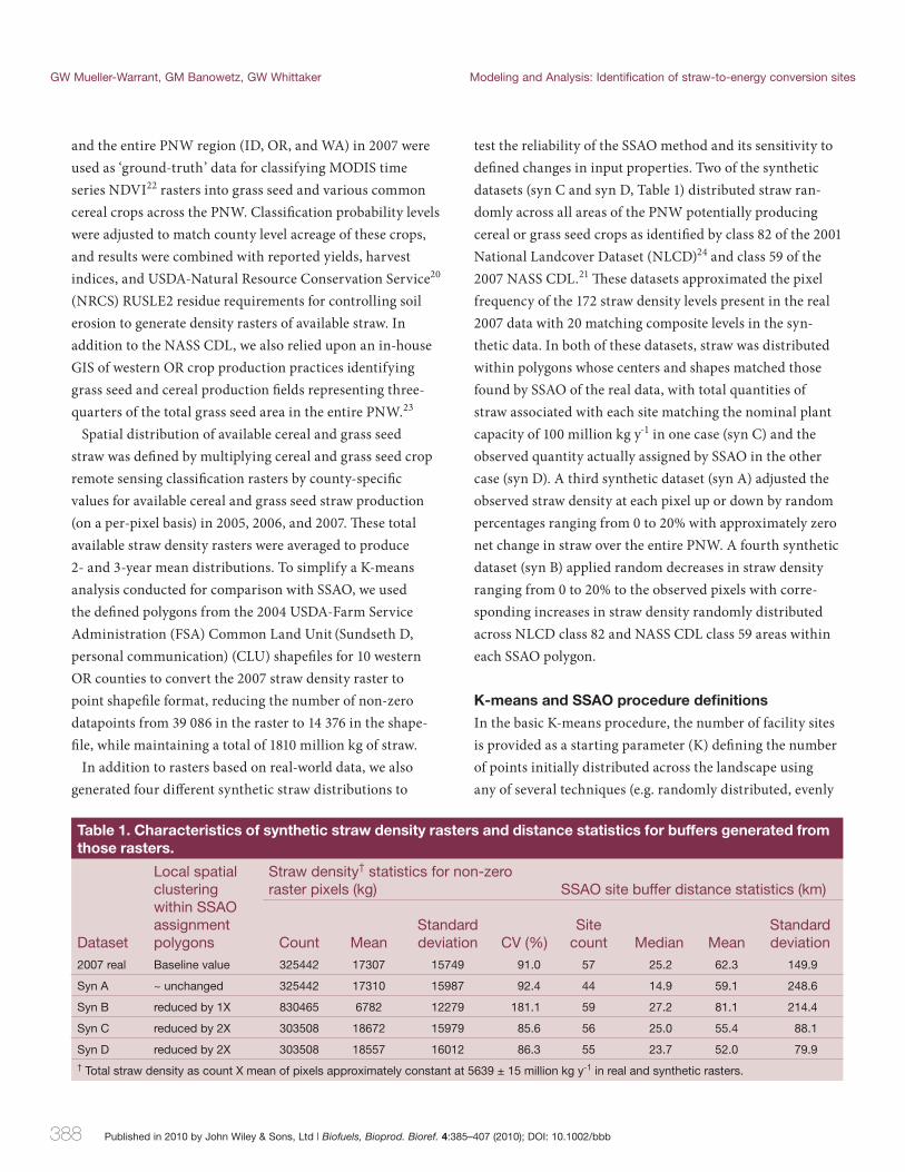
test the reliability of the SSAO method and its sensitivity to defi ned changes in input properties. Two of the synthetic datasets (syn C and syn D, Table 1) distributed straw ran-domly across all areas of the PNW potentially producing cereal or grass seed crops as identifi ed by class 82 of the 2001 National Landcover Dataset (NLCD)24 and class 59 of the 2007 NASS CDL.21 Th ese datasets approximated the pixel frequency of the 172 straw density levels present in the real 2007 data with 20 matching composite levels in the syn-thetic data. In both of these datasets, straw was distributed within polygons whose centers and shapes matched those found by SSAO of the real data, with total quantities of straw associated with each site matching the nominal plant capacity of 100 million kg y-1 in one case (syn C) and the observed quantity actually assigned by SSAO in the other case (syn D). A third synthetic dataset (syn A) adjusted the observed straw density at each pixel up or down by random percentages ranging from 0 to 20% with approximately zero net change in straw over the entire PNW. A fourth synthetic dataset (syn B) applied random decreases in straw density ranging from 0 to 20% to the observed pixels with corre-sponding increases in straw density randomly distributed across NLCD class 82 and NASS CDL class 59 areas within each SSAO polygon.
K-means and SSAO procedure defi nitions
In the basic K-means procedure, the number of facility sites is provided as a starting parameter (K) defi ning the number of points initially distributed across the landscape using any of several techniques (e.g. randomly distributed, evenly
Table 1. Characteristics of synthetic straw density rasters and distance statistics for buffers generated from those rasters.
Dataset
Local spatial clustering within SSAO assignment polygons
Straw density† statistics for non-zero raster pixels (kg) SSAO site buffer distance statistics (km)
Count MeanStandard deviation CV (%)
Site count Median Mean
Standard deviation
2007 real Baseline value 325442 17307 15749 91.0 57 25.2 62.3 149.9
Syn A ~ unchanged 325442 17310 15987 92.4 44 14.9 59.1 248.6
Syn B reduced by 1X 830465 6782 12279 181.1 59 27.2 81.1 214.4
Syn C reduced by 2X 303508 18672 15979 85.6 56 25.0 55.4 88.1
Syn D reduced by 2X 303508 18557 16012 86.3 55 23.7 52.0 79.9† Total straw density as count X mean of pixels approximately constant at 5639 ± 15 million kg y-1 in real and synthetic rasters.
Published in 2010 by John Wiley & Sons, Ltd | Biofuels, Bioprod. Bioref. 4:385–407 (2010); DOI: 10.1002/bbb 389
Modeling and Analysis: Identification of straw-to-energy conversion sites GW Mueller-Warrant, GM Banowetz, GW Whittaker
spaced on a grid, or in a pattern based on some preceding analysis). Data representing the variable of interest, whether customer request points in service facility siting or available straw in bioenergy plant siting, must have a spatial location and may have an optional weight corresponding to factors such as the number of service calls per address or the quan-tity of straw present per pixel or per fi eld. Th ese data points are assigned temporary membership to the nearest facility site, and the mean center of all points assigned to each initial facility site location is calculated, using optional weights as desired. In the next round of the cycle, the mean centers cal-culated in the previous round are used as the new locations of the K facility sites, and the cycle repeats until site loca-tions stabilize (or equivalently, resource points stop chang-ing which facility site they are assigned to). In the original formulation of the K-means method, the factor minimized was the sum of the weights times the squared distances between data points and sites, but persuasive arguments exist that it is better to use simple linear distance rather than squared distance.12 Linear distance simplifi ed our calcula-tions. Several characteristics stand out in K-means analysis. First, while the number of sites is fi xed, the number of points (or quantity of the resource factor in question) assigned to each site can be highly variable. Second, depending on the strength of spatial clustering present in the data, the fi nal site positions may be highly sensitive to the arbitrary or random facility site distribution initially assumed. Consequently, K-means only guarantees global rather than simply local optimization of site positions if it is run multi-ple times from diff erent initial starting seed patterns where the run with the lowest total clustering error is selected.
A major issue in use of K-means is size of the datasets under analysis. Our straw density dataset for 2007 com-prised 5632 million kg straw at 303 508 unique 250-m by 250-m non-zero pixels in synthetic dataset D, and at 325 442 unique non-zero pixels in the raw data. Analyses reported by Zarzani12 used maximums of 5000 data points and 40 clus-ters. As computational complexity of K-means scales with N*K, our analysis of 57 sites and 325 442 non-zero straw-containing pixels is potentially over 90 times as diffi cult as Zarzani’s. One method to reduce the complexity would be to merge data from neighboring pixels into actual fi elds on which grass seed and cereal crops were grown. Since the
average straw density of non-zero pixels was 17 307 kg per 6.25 ha, grouping pixels into fi elds with an average size of 62.5 ha would reduce the computational complexity to only 9 times that encountered by Zarzani. A fi eld size of 62.5 ha is 3.4 times the average fi eld size for grass seed crops, but rea-sonably close to the average size for cereal fi elds across the PNW. Recent removal of the CLU polygons from the public record greatly complicated the steps it would take to convert our pixel-based straw yield data to agricultural fi eld-based data. Hence we were only able to simplify the data in west-ern OR counties for which we had obtained CLU polygons24 prior to their removal from public record.
Our SSAO procedure defi ned the number of facility sites (K) indirectly through a combination of the total avail-able straw in the PNW and the nominal capacity of plants designed on the basis of diff erent models of potential bioenergy conversion processes. Th e farm-sized pilot project was designed as a syngas powered electrical generator with a nominal capacity of 1 million kg y-1, roughly corresponding to the total quantity of straw a typical grass seed producer in that region has to manage. Th e largest capacity plant (100 million kg y-1) corresponds to an industrial park version in western OR currently in fi nal stages of design specifi cation, site selection, funding acquisition, and permitting for fer-mentation-based production of ethanol and other biofuels. It is also similar in size to the distributed network of fast pyrolysis plants proposed for Germany.8 Th e intermediate scale capacity (10 million kg y-1) represents the combined straw production from several farms, and could be viewed as a series of distributed bio-oil production sites with railway access to ship product to large, centralized refi neries, or it could represent a scaling-up of the syngas technology. For all three plant sizes, some fl exibility exists in how close to nominal plant capacity the actual straw supply is, but the envisioned technologies clearly operate on diff erent scales and would benefi t from reasonably stable matches between nominal capacity and annually available straw.
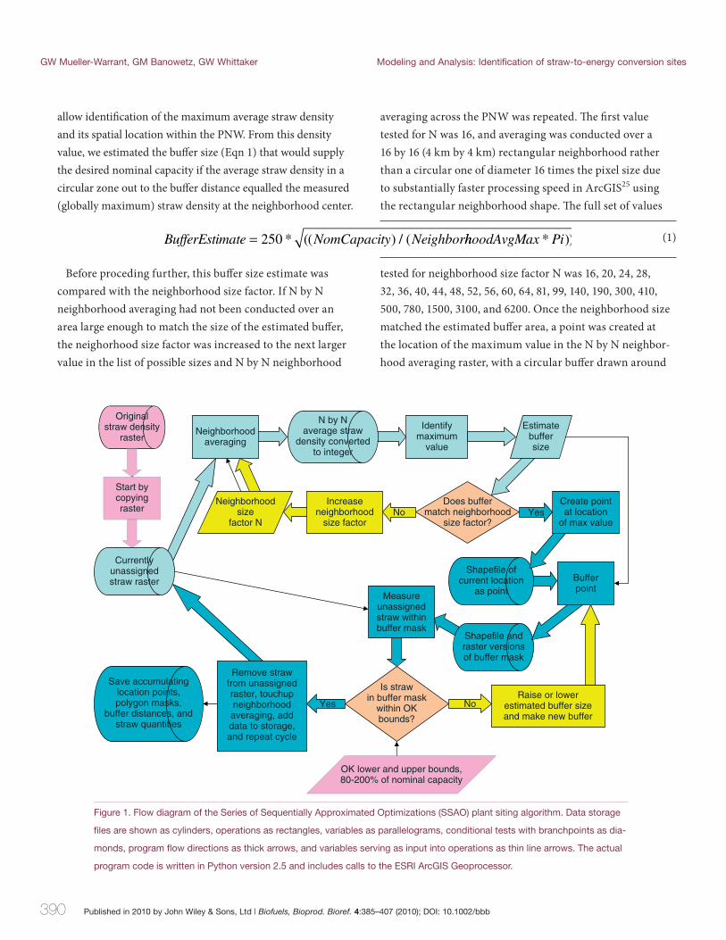
Th e fi rst step in the SSAO process was to set the nominal plant capacity, indirectly defi ning the total number of sites. Th e original straw density raster was copied to a target direc-tory where it served as the starting version of the currently unassigned straw raster (Fig. 1). Th e unassigned straw raster was then subjected to N by N neighborhood averaging to
390 Published in 2010 by John Wiley & Sons, Ltd | Biofuels, Bioprod. Bioref. 4:385–407 (2010); DOI: 10.1002/bbb
GW Mueller-Warrant, GM Banowetz, GW Whittaker Modeling and Analysis: Identification of straw-to-energy conversion sites
allow identifi cation of the maximum average straw density and its spatial location within the PNW. From this density value, we estimated the buff er size (Eqn 1) that would supply the desired nominal capacity if the average straw density in a circular zone out to the buff er distance equalled the measured (globally maximum) straw density at the neighborhood center.
averaging across the PNW was repeated. Th e fi rst value tested for N was 16, and averaging was conducted over a 16 by 16 (4 km by 4 km) rectangular neighborhood rather than a circular one of diameter 16 times the pixel size due to substantially faster processing speed in ArcGIS25 using the rectangular neighborhood shape. Th e full set of values
Figure 1. Flow diagram of the Series of Sequentially Approximated Optimizations (SSAO) plant siting algorithm. Data storage
fi les are shown as cylinders, operations as rectangles, variables as parallelograms, conditional tests with branchpoints as dia-
monds, program fl ow directions as thick arrows, and variables serving as input into operations as thin line arrows. The actual
program code is written in Python version 2.5 and includes calls to the ESRI ArcGIS Geoprocessor.
(1)BufferEstimate NomCapacity Neighbor= 250 * (( ) / ( hhoodAvgMax Pi* ))
Before proceding further, this buff er size estimate was compared with the neighborhood size factor. If N by N neighborhood averaging had not been conducted over an area large enough to match the size of the estimated buff er, the neighorhood size factor was increased to the next larger value in the list of possible sizes and N by N neighborhood
tested for neighborhood size factor N was 16, 20, 24, 28, 32, 36, 40, 44, 48, 52, 56, 60, 64, 81, 99, 140, 190, 300, 410, 500, 780, 1500, 3100, and 6200. Once the neighborhood size matched the estimated buff er area, a point was created at the location of the maximum value in the N by N neighbor-hood averaging raster, with a circular buff er drawn around
Published in 2010 by John Wiley & Sons, Ltd | Biofuels, Bioprod. Bioref. 4:385–407 (2010); DOI: 10.1002/bbb 391
Modeling and Analysis: Identification of straw-to-energy conversion sites GW Mueller-Warrant, GM Banowetz, GW Whittaker
that point using a radius equal to the estimated buff er size. A raster mask version of the polygon buff er was used to measure the quantity of currently unassigned straw within the buff er zone, and this was tested against lower and upper limits of 80 and 200% of the nominal plant capacity. If the quantity of straw fell below or above those accepted limits, the estimated buff er size was adjusted slightly and measure-ment of unassigned straw within the buff er was repeated until values were within acceptable boundaries. When that occurred, straw in the buff er area was removed from the currently unassigned straw raster and the buff er center points, polygons, distances, and straw quantities were saved to permanent fi les. In a fi nal clean-up step, N by N neighbor-hood averaging centered on the most recently defi ned plant site was conducted over twice the current neighborhood averaging distance plus the buff er radius, and results were merged back into a revised version of the full N by N neigh-borhood averaging raster. Th e overall process repeated until all straw had been assigned or the quantity remaining unas-signed became less than 80% of nominal plant capacity. Th e most computationally intensive aspect to SSAO was the N by N neighborhood averaging step, and indeed neighborhood averaging became very slow for N >= 64 and failed to fi nish execution for N > 100 in rasters covering the PNW at 250 m resolution. We handled cases of N >= 64 by adding interme-diate block analyses that gradually coarsened the resolution of the unassigned straw raster in the sequence of 3, 5, 7, 9, 13, 25, 51, and 99 times 250 m. While all locations for 100 million kg straw per year capacity plants could be identi-fi ed within a little over an hour of computer run time, the 10 million kg capacity plants required nearly a day to run, and the 1 million kg capacity plants required approximately one week. Python scripts included tests that allowed semiau-tomatic resumption of runs interrupted by system crashes, power failures, or deliberate user intervention.
Results and Discussion
Validation of SSAO and comparison with K-means
One question to be considered was whether the individual site locations and collection assignment regions produced by SSAO were optimized relative to the straw distribu-tion patterns present at each step in the assignment cycle.
Optimization in the K-means sense as commonly used10,12,13 would require that the weighted mean center of all straw assigned to a specifi c plant site be identical to the SSAO site location (or center of the corresponding collection region circular polygon). By defi nition of K-means, the sum of the weighted distances (or distances squared in the original version) to any other location is greater than the sum to the K-means center. For a simplifi ed version of the comparison of SSAO with K-means, consider a circular polygon around a central point with uniform density of straw within it, and concentric rings of decreasing straw density outside the cen-tral disk. If the total straw present inside the central circle is less than or equal to the amount needed to supply a con-version plant, the least cost (least total transport distance) optimum location for the plant is the center point. But the center point is also the local maximum of the N by N neigh-borhood averaging raster whenever N is large enough that the neighborhood distance equals or exceeds the radius of the inner circle. If the total straw within the central circle is greater than the plant’s capacity, multiple equally optimal locations would exist inside the central circle within some distance from the central point.
Th e assumption of uniformity in straw density within the concentric circles can be relaxed by introducing an error term the size of whose average random fl uctuations is in the order of the diff erence in straw yields between adjacent concentric circles. If the number of pixels within each concentric circle >> 1, positions of both the N by N neigh-borhood averaging maxima and the K-means clustering point will approach the same original center point, and the discrepancies in position can be made arbitrarily small by increasing the number of pixels within each concentric cir-cle. Th is does not prove that N by N neighborhood averaging and K-means clustering identify identical positions when modest levels of error are present, but indicates that both tend to move toward the same central location as number of pixels increases and/or size of error term decreases.
In real world conditions, straw distribution is not uniform within concentric circles, but exists in two or more distinct fi elds separated by regions with less (or no) straw. For the case of two fi elds each possessing 50% of the amount of straw needed to operate the plants, N by N neighborhood averag-ing and K-means clustering (for K = 1) both pick points on
392 Published in 2010 by John Wiley & Sons, Ltd | Biofuels, Bioprod. Bioref. 4:385–407 (2010); DOI: 10.1002/bbb
GW Mueller-Warrant, GM Banowetz, GW Whittaker Modeling and Analysis: Identification of straw-to-energy conversion sites
the line connecting the two fi elds as optimum locations to minimize total transport cost. If one fi eld has more straw than the second, or a third equal sized-fi eld is present shar-ing the total straw needed to meet a single plant’s nominal capacity, the weighted mean centers of the points will match the sites identifi ed by both K-means (for K = 1) and SSAO. Similar arguments can extend the proof to arbitrary num-bers of fi elds within a circular region whose total quantity of straw matches that needed by a single conversion plant.
Before analyzing overlap among spatial clusters as it aff ects SSAO and K-means (for K > 1), eff ects of the approximations made in SSAO to speed up the computational process need to be considered. Th e use of rectangular rather than circular neighborhood shapes and the limiting of N to specifi c dis-crete values in N by N neighborhood averaging introduce potential mismatch between maxima in the neighborhood averaging raster (and derived estimates for buff er distances) and the quantity of straw actually found within the buff er mask area of the unassigned straw raster. Several methods can be used to quantify this mismatch and characterize its impact on site locations. Th e simplest is to examine the SSAO log fi les to see how oft en it was necessary to change the buff er size from its originally estimated value, one based on the assumption of uniform straw density near the location of the neighborhood averaging maxima. For the 100 million kg y-1 capacity plants based on 2007 straw distribution, the fi rst 33 out of 57 plant sites, and a total of 47, required no adjustment to buff er size from the initial value based on the maxima in the neighborhood averaging rasters. For the 10 million kg y-1 capacity plants based on 2007 straw distribu-tion, no adjustment to buff er size was needed for 535 out of 596 sites. For the 1 million kg y-1 capacity plants based on 2007 straw distribution, no adjustment to buff er size was needed for 3377 out of 5081 sites. Most of the larger buff er size adjustments (those > 2X) that were made occurred near the end of the SSAO site selection process. For example, 63% of the buff er adjustments larger than 2X occurred while sit-ing the fi nal 20% of the 1 million kg y-1 plants.
A second method to quantify the mismatch was to compare the siting event order with the ranking of buff er distances. For the 100 million kg y-1 capacity plants, it was possible to determine the exact number of out-of-order siting events by visual inspection. For SSAO of the 2007 straw density, 9 of the
57 sites were out of order, and Pearson’s correlation of ranked orders (equivalent to Spearman’s rho) was 0.994. For SSAO of the 1 and 10 million kg y-1 capacity plants, Pearson’s ranked correlations were 0.942 and 0.978 in 2007, with similar results for the other years. If a slightly more accurate enumeration of plant sites was desired for planning purposes, ranking of buff er sizes could be used in place of SSAO siting event order.
A third method to quantify the mismatch was to conduct weighted mean center calculations of straw assigned to each site and measure distances between those positions and the corresponding original polygon centers. When this was done for sites based on 2007 straw density with plant capacities of 1, 10, and 100 million kg y-1, the off set between the SSAO site locations and the weighted mean centers of the straw assigned to them was less than 20% of the individual buff er distances in 60.0, 86.7, and 84.2% of cases. For the most consistently assigned 25% of sites at each of these three capacities, off sets averaged only 6.2, 3.3, and 3.2% of buff er distances. Average off sets increased to 13.5, 7.0, and 6.9% of buff er distances for the second-best quarter and to 21.5, 12.0, and 13.4% for the third-best quarter of sites. While these measurements showed that our implementation of SSAO was less than perfect in optimizing site locations, discrepancies between weighted mean centers and our site locations were on the order of typical rural road spacings (1.6 km) for all three plant capaci-ties, and are of little practical signifi cance. If circumstances existed in which such relatively small diff erences in position were important, it would be simple to substitute the weighted mean centers for the original neighborhood averaging maxima locations as a fi nal step in the plant siting process, increasing the total computational time by about 50%.
Based on previously discussed theoretical considera-tions and the measured performance of SSAO, it is clear that SSAO and K-means behave similarly if the underlying data are strongly clustered into spatially distinct aggrega-tions that are similarly sized in terms of the total resource of interest present within each cluster. Th is is true as long as the product of K (from K-means) and capacity (from SSAO) equals the total resource present across the entire area. Major questions of interest are how and when SSAO and K-means diff er if signifi cant overlap exists among the underly-ing clusters or the clusters possess widely diff ering resource totals. In general, K-means sites will be well separated from
Published in 2010 by John Wiley & Sons, Ltd | Biofuels, Bioprod. Bioref. 4:385–407 (2010); DOI: 10.1002/bbb 393
Modeling and Analysis: Identification of straw-to-energy conversion sites GW Mueller-Warrant, GM Banowetz, GW Whittaker
each other and total resource assignment may vary consider-ably among them. In contrast, some of the SSAO sites may be very close to each other, diff ering mainly in their order of creation and size of assignment areas. Resources assigned to each SSAO site will, by design, be similar for all sites. Th e later-assigned polygons in SSAO may resemble ‘donuts’ for simple cases with only two nearly coincident plant sites and ‘Swiss cheese’ for complex cases with many overlaps.
To examine the implications of these diff erences between K-means and SSAO, we conducted K-means facility siting analysis for 2007 straw density in 10 western OR counties using K = 18 and the fi rst 18 SSAO plant sites in western OR from the 100 million kg y-1 capacity analysis as starting facil-ity positions. One diff erence between the two approaches was that the variance in straw assignment per site was 55% higher for K-means than for SSAO, with 60% of the total straw for K-means being assigned to the fi rst 50% of sites in their order of creation by SSAO. Weighted mean transport distance as defi ned in Eqn 2 is directly proportional to cost of transporting straw to the associated processing site.
WeightedTransDist = Σ (StrawDensity ∗Dist)/ Σ StrawDensity (2)
Th is value can be converted to mean straw density across the site collection area using Eqn 3 to provide a measurement inversely proportional to transport cost per unit of straw or directly proportional to effi ciency of siting methods in defi ning good plant locations.
MeanStrawDensity = Σ StrawDensity / (4∗Pi∗WeightedTransDis) (3)
A major diff erence between SSAO and K-means plant siting methods was that the mean straw density in areas assigned to the fi rst eight plants (in SSAO site creation order) was 26% higher using SSAO than K-means. For the next seven plants, mean straw densities were similar for both methods. For the fi nal three plants, mean straw densities were much greater for K-means than for SSAO. Totalled over all sites, mean straw densities for K-means were 54% higher than for SSAO. Simply put, K-means did a superior job of optimizing site locations in a global sense, i.e. using up all of the resources, assigning all of the straw to plants. SSAO did a superior job of optimizing site locations in a sequential
(fi rst come, fi rst served) sense for the fi rst 44% of sites while matching the performance of K-means for the next 39%. Th e overall superiority of SSAO for the fi rst 83% of sites came at a cost of failing to effi ciently assign the last 17% of straw. Leaving 17% of customers as ‘orphans’ without service would be an unacceptable design for utilities such as tele-phones or electric power. In the case of agriculture and other natural resource extraction industries, it would be unreal-istic to assume that the playing fi eld is (or ought to be) truly level. Just as some physical fi elds are higher yielding than others due to more fertile soils or better rainfall patterns, so too will some fi elds possess advantages over others in terms of nearness to sites at which conversion plants are sited. Entrepeneurs are unlikely to accept 20 to 30% increases in transportation costs just to insure that their future competi-tors will have good locations left to choose from, unless they have strong reasons to believe that they will gain control of the industry in a de facto monopoly.
Sensitivity of SSAO to simulated differences in
straw distribution patterns
Th e four synthetic datasets we developed all matched the general global distribution of straw across the PNW in 2007. Th ese datasets can most simply be viewed as testing either: (1) the impact of variation in spatial aggregation of straw on a local scale (i.e. within the original SSAO straw assign-ment polygons); (2) the impact of random error in straw density levels; or (3) combination of both factors. Compared to results from the real 2007 straw data for a plant capac-ity of 100 million kg of straw y-1, the total number of sites found by SSAO for the synthetic datasets was within two of the number of sites for the real data in 75% of the synthetic dataset analyses (Table 1). Th e number of sites dropped from 57 to 44 for synthetic dataset A, in which the only change was a random increase or decrease in straw density averag-ing 10% at the original 2007 data points. While the mean buff er distance for this synthetic dataset was similar to that for the real data, the median buff er distance dropped to 59% of the value from the real data while the standard devia-tion increased by 66%. While these changes could certainly have been minimized by tightening the upper and lower boundaries of the straw quantity test within SSAO, they do indicate that our methods were very sensitive to random
394 Published in 2010 by John Wiley & Sons, Ltd | Biofuels, Bioprod. Bioref. 4:385–407 (2010); DOI: 10.1002/bbb
GW Mueller-Warrant, GM Banowetz, GW Whittaker Modeling and Analysis: Identification of straw-to-energy conversion sites
resource level changes in regards to the fi nal quarter of all plant site assignments. In contrast to synthetic dataset A, datasets C and D reduced the local spatial clustering while leaving variability in straw density values relatively unchanged from the real data. Both median and mean buff er distances for datasets C and D were close to results from the real data, while their standard deviations were smaller. Because the hypothetical straw in these two datasets was more uniformly distributed across the original assignment regions than the real straw had been, SSAO was less sensitive to inclusion or exclusion of specifi c high straw density pixels near the periphery of each site’s buff er. Synthetic dataset B can be viewed as possessing a mixture of the properties of synthetic datasets A and D, and dataset B was most similar to dataset A in standard deviation of buff er distances while causing an increase in mean buff er distances beyond that of the real data. Th e only diff erence between datasets C and D was whether the total straw within the original assignment polygons was scaled to match to the exact nominal capacity (case C) or the observed quantity assigned to sites (case D). Th is diff erence had little impact on buff er distance statistics.
When we attempted to manually match assignment areas from SSAO of the synthetic datasets with those from analysis of the real 2007 data based on similarity in plant site posi-tions and buff er distances, the matchup process had fewer ambigities for dataset syn D than for syn A, B, or C. For dataset syn D and the real 2007 data, overlap in total straw assigned to matching polygons exceeded 50% in 47 out of 55 sites. Indeed, the overlap exceeded 60, 70, 80, and 90% of total straw in 42, 34, 25, and 21 of the 55 matchups when measured using the synthetic straw. Overlaps for the fi rst half of all site assignments averaged 86%, ranging from 52 to 100% of total straw. Overlaps for the fi rst 80% of all site assignments aver-aged 81% and ranged from 32 to 100%. Overlap measure-ments were only slightly poorer when the real 2007 data were used rather than synthetic dataset D. Off set distances between matching plant sites from SSAO of synthetic dataset D and of the real 2007 straw density data confi rmed our fi ndings that the SSAO method produced highly stable results for the fi rst 75% of plants sited along with considerable volatility in siting of the fi nal 25%. Mean off sets for the fi rst 25, 50, and 75% of all plants sited averaged 5.0, 7.1, and 9.7 km, or 28, 35, and 40% of the corresponding mean buff er distances. Th e median off set for all 55 matchups was 6.0 km, while the mean value
was 34 km, refl ecting the very large distances needed to align the last few site assignments from the two analyses.
Spatial distribution of available straw relative to
capacity of bioenergy conversion plants
Bioenergy conversion plants with capacities on the order of 1 million kg of straw y-1 have been proposed as a technologi-cally achievable means to increase on-farm income and pro-duce renewable energy utilizing resources that are already being produced.1 Approximately 6200 such plants distrib-uted across the PNW would be required to convert the annually available straw into fuel or electricity. While many obstacles exist to the construction and operation of these plants, common concerns impacting their operation include the low physical density of straw, costs inherent in collecting and compressing straw in the fi eld, and expenses in hauling straw to processing facilities. Weighing against higher trans-portation costs for bringing straw greater distances to larger, more centralized processing plants are possible economies of scale in those larger plants. Regardless of plant scale, it is likely that transportation costs and density of available straw across the landscape will strongly infl uence economic viabil-ity and optimal plant locations. Plants can be expected to be built and brought into operation in a serial manner, begin-ning at ‘prime’ sites chosen by the early adoptors. Th e siting of early plants may impact the amount of straw available in adacent sites and limit subsequent development.
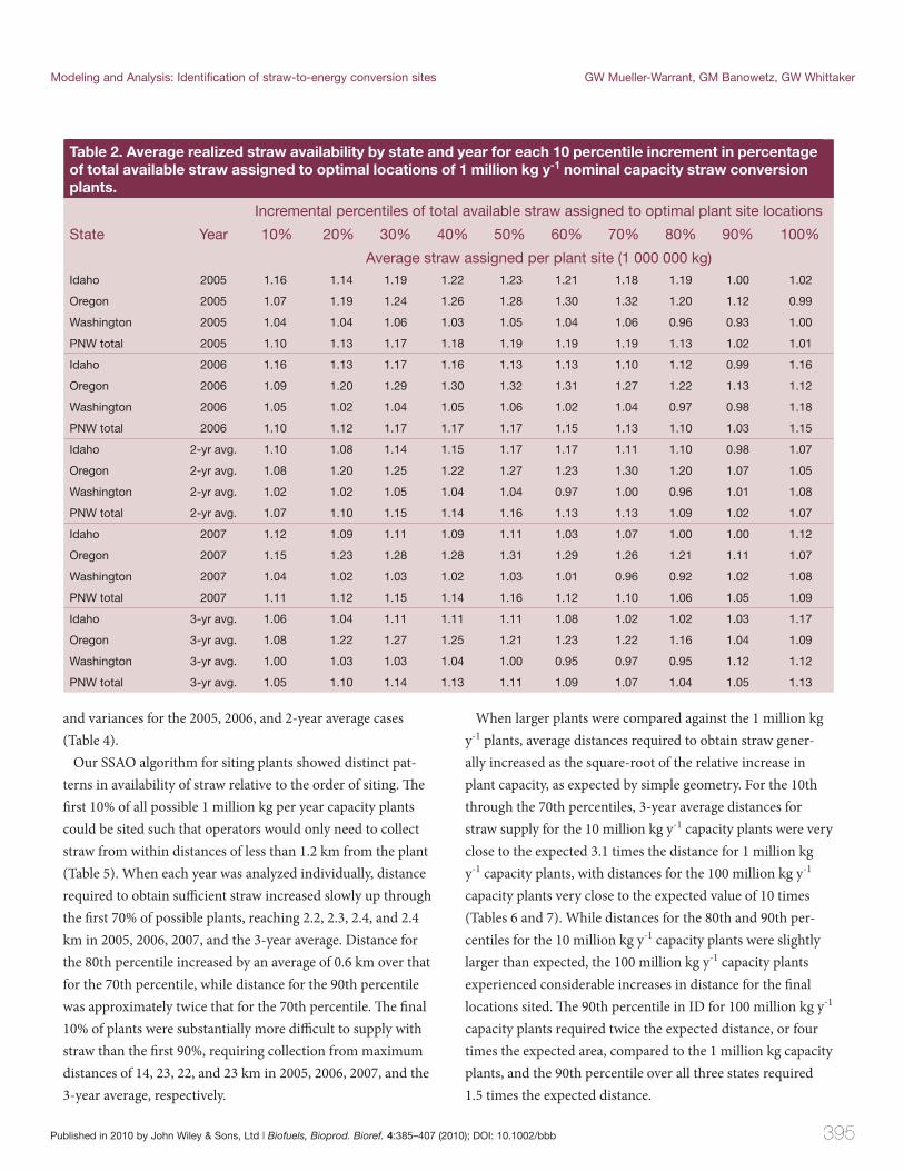
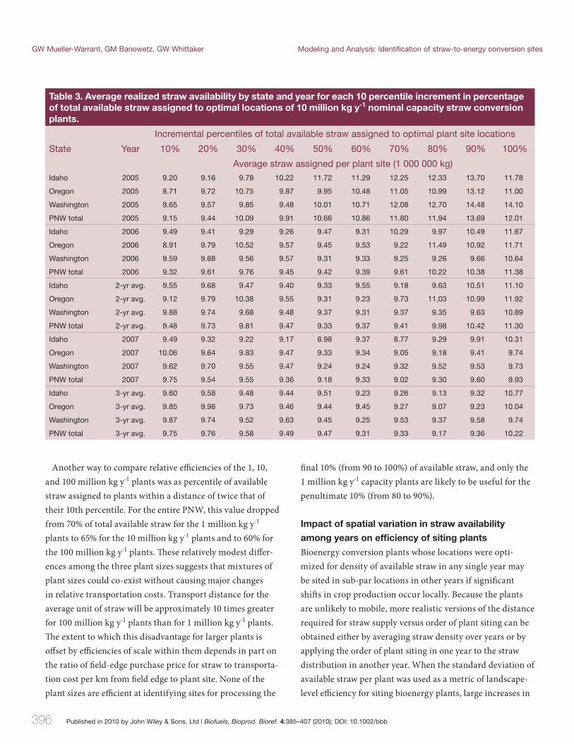
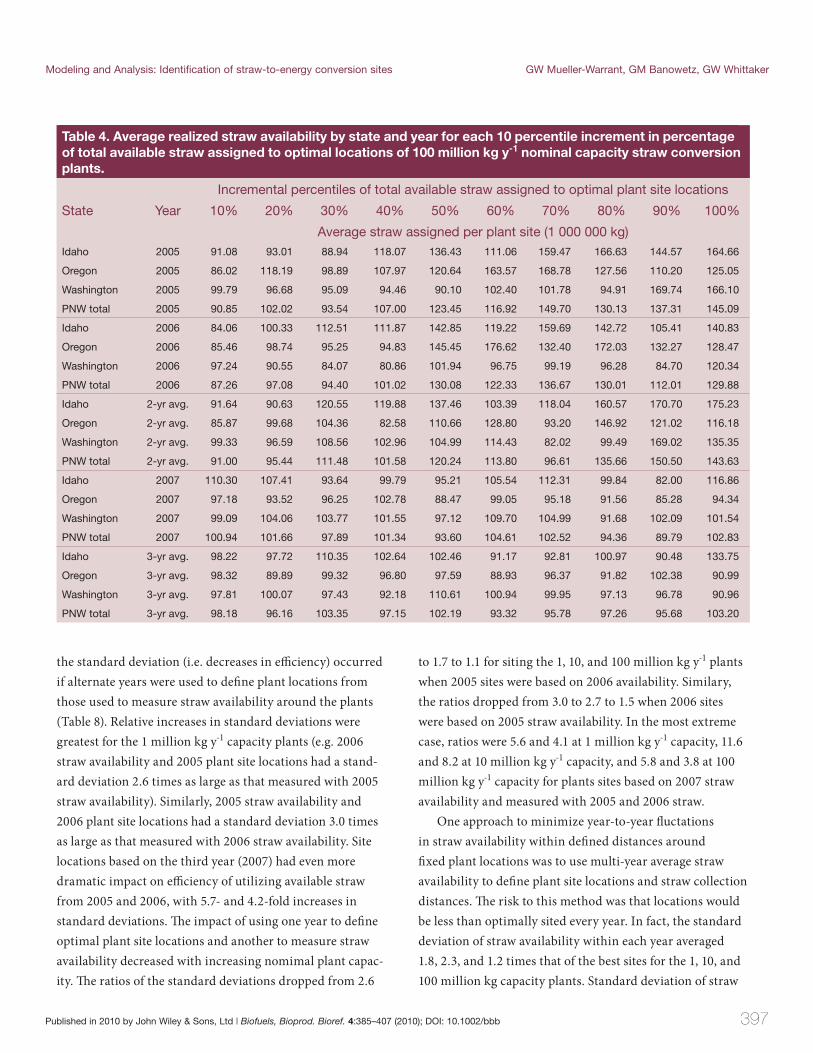
Despite the fact that the SSAO iterative process only required available straw to provide between 80 and 200% of nominal plant capacity, our algorithm for siting individual plants at the center of the highest density of remaining straw identifi ed sites where available straw averaged only slightly above or below nominal capacities. Th e 1 million kg y-1 nomi-nal capacity plants averaged 1.09 million kg y-1 of realized straw for the 3-year average raster over the entire PNW, with generally similar results in other years when subdivided into states (Table 2). When the 10 million kg y-1 nominal capacity plants were considered, the average realized straw was also close to the nominal capacity, averaging 10.96, 9.85, 9.46, and 9.54 million kg y-1 of straw for 2005, 2006, 2007, and the 3-year average for the entire PNW (Table 3). For the the 100 million kg y-1 nominal capacity plants across the PNW, average realized straw for 2007 and the 3-year average was 98.4 and 98.2 million kg y-1, respectively, with larger means
Published in 2010 by John Wiley & Sons, Ltd | Biofuels, Bioprod. Bioref. 4:385–407 (2010); DOI: 10.1002/bbb 395
Modeling and Analysis: Identification of straw-to-energy conversion sites GW Mueller-Warrant, GM Banowetz, GW Whittaker
and variances for the 2005, 2006, and 2-year average cases (Table 4).
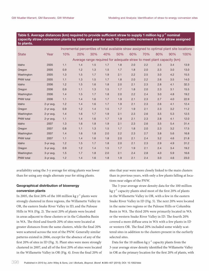
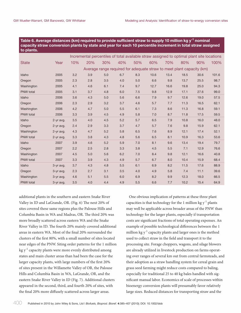
Our SSAO algorithm for siting plants showed distinct pat-terns in availability of straw relative to the order of siting. Th e fi rst 10% of all possible 1 million kg per year capacity plants could be sited such that operators would only need to collect straw from within distances of less than 1.2 km from the plant (Table 5). When each year was analyzed individually, distance required to obtain suffi cient straw increased slowly up through the fi rst 70% of possible plants, reaching 2.2, 2.3, 2.4, and 2.4 km in 2005, 2006, 2007, and the 3-year average. Distance for the 80th percentile increased by an average of 0.6 km over that for the 70th percentile, while distance for the 90th percentile was approximately twice that for the 70th percentile. Th e fi nal 10% of plants were substantially more diffi cult to supply with straw than the fi rst 90%, requiring collection from maximum distances of 14, 23, 22, and 23 km in 2005, 2006, 2007, and the 3-year average, respectively.
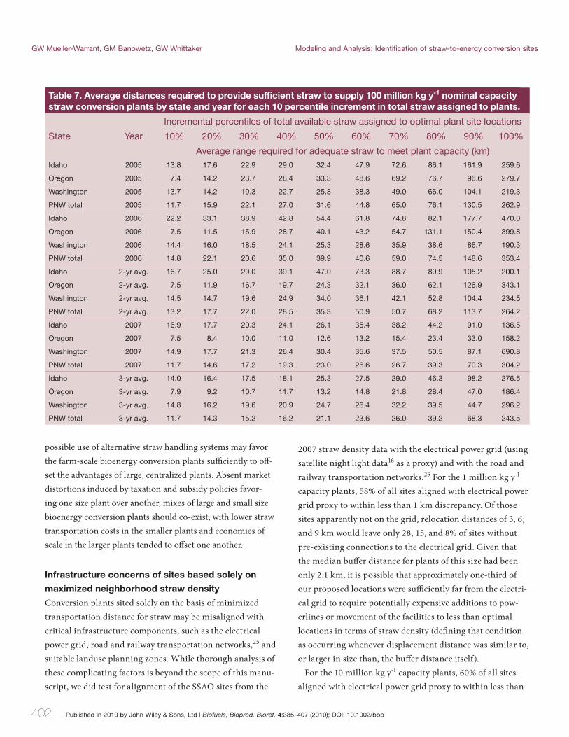
When larger plants were compared against the 1 million kg y-1 plants, average distances required to obtain straw gener-ally increased as the square-root of the relative increase in plant capacity, as expected by simple geometry. For the 10th through the 70th percentiles, 3-year average distances for straw supply for the 10 million kg y-1 capacity plants were very close to the expected 3.1 times the distance for 1 million kg y-1 capacity plants, with distances for the 100 million kg y-1 capacity plants very close to the expected value of 10 times (Tables 6 and 7). While distances for the 80th and 90th per-centiles for the 10 million kg y-1 capacity plants were slightly larger than expected, the 100 million kg y-1 capacity plants experienced considerable increases in distance for the fi nal locations sited. Th e 90th percentile in ID for 100 million kg y-1 capacity plants required twice the expected distance, or four times the expected area, compared to the 1 million kg capacity plants, and the 90th percentile over all three states required 1.5 times the expected distance.
Table 2. Average realized straw availability by state and year for each 10 percentile increment in percentage of total available straw assigned to optimal locations of 1 million kg y-1 nominal capacity straw conversion plants.
Incremental percentiles of total available straw assigned to optimal plant site locations
State Year 10% 20% 30% 40% 50% 60% 70% 80% 90% 100%
Average straw assigned per plant site (1 000 000 kg)Idaho 2005 1.16 1.14 1.19 1.22 1.23 1.21 1.18 1.19 1.00 1.02
Oregon 2005 1.07 1.19 1.24 1.26 1.28 1.30 1.32 1.20 1.12 0.99
Washington 2005 1.04 1.04 1.06 1.03 1.05 1.04 1.06 0.96 0.93 1.00
PNW total 2005 1.10 1.13 1.17 1.18 1.19 1.19 1.19 1.13 1.02 1.01
Idaho 2006 1.16 1.13 1.17 1.16 1.13 1.13 1.10 1.12 0.99 1.16
Oregon 2006 1.09 1.20 1.29 1.30 1.32 1.31 1.27 1.22 1.13 1.12
Washington 2006 1.05 1.02 1.04 1.05 1.06 1.02 1.04 0.97 0.98 1.18
PNW total 2006 1.10 1.12 1.17 1.17 1.17 1.15 1.13 1.10 1.03 1.15
Idaho 2-yr avg. 1.10 1.08 1.14 1.15 1.17 1.17 1.11 1.10 0.98 1.07
Oregon 2-yr avg. 1.08 1.20 1.25 1.22 1.27 1.23 1.30 1.20 1.07 1.05
Washington 2-yr avg. 1.02 1.02 1.05 1.04 1.04 0.97 1.00 0.96 1.01 1.08
PNW total 2-yr avg. 1.07 1.10 1.15 1.14 1.16 1.13 1.13 1.09 1.02 1.07
Idaho 2007 1.12 1.09 1.11 1.09 1.11 1.03 1.07 1.00 1.00 1.12
Oregon 2007 1.15 1.23 1.28 1.28 1.31 1.29 1.26 1.21 1.11 1.07
Washington 2007 1.04 1.02 1.03 1.02 1.03 1.01 0.96 0.92 1.02 1.08
PNW total 2007 1.11 1.12 1.15 1.14 1.16 1.12 1.10 1.06 1.05 1.09
Idaho 3-yr avg. 1.06 1.04 1.11 1.11 1.11 1.08 1.02 1.02 1.03 1.17
Oregon 3-yr avg. 1.08 1.22 1.27 1.25 1.21 1.23 1.22 1.16 1.04 1.09
Washington 3-yr avg. 1.00 1.03 1.03 1.04 1.00 0.95 0.97 0.95 1.12 1.12
PNW total 3-yr avg. 1.05 1.10 1.14 1.13 1.11 1.09 1.07 1.04 1.05 1.13
396 Published in 2010 by John Wiley & Sons, Ltd | Biofuels, Bioprod. Bioref. 4:385–407 (2010); DOI: 10.1002/bbb
GW Mueller-Warrant, GM Banowetz, GW Whittaker Modeling and Analysis: Identification of straw-to-energy conversion sites
Another way to compare relative effi ciencies of the 1, 10, and 100 million kg y-1 plants was as percentile of available straw assigned to plants within a distance of twice that of their 10th percentile. For the entire PNW, this value dropped from 70% of total available straw for the 1 million kg y-1 plants to 65% for the 10 million kg y-1 plants and to 60% for the 100 million kg y-1 plants. Th ese relatively modest diff er-ences among the three plant sizes suggests that mixtures of plant sizes could co-exist without causing major changes in relative transportation costs. Transport distance for the average unit of straw will be approximately 10 times greater for 100 million kg y-1 plants than for 1 million kg y-1 plants. Th e extent to which this disadvantage for larger plants is off set by effi ciencies of scale within them depends in part on the ratio of fi eld-edge purchase price for straw to transporta-tion cost per km from fi eld edge to plant site. None of the plant sizes are effi cient at identifying sites for processing the
fi nal 10% (from 90 to 100%) of available straw, and only the 1 million kg y-1 capacity plants are likely to be useful for the penultimate 10% (from 80 to 90%).
Impact of spatial variation in straw availability
among years on effi ciency of siting plants
Bioenergy conversion plants whose locations were opti-mized for density of available straw in any single year may be sited in sub-par locations in other years if signifi cant shift s in crop production occur locally. Because the plants are unlikely to mobile, more realistic versions of the distance required for straw supply versus order of plant siting can be obtained either by averaging straw density over years or by applying the order of plant siting in one year to the straw distribution in another year. When the standard deviation of available straw per plant was used as a metric of landscape-level effi ciency for siting bioenergy plants, large increases in
Table 3. Average realized straw availability by state and year for each 10 percentile increment in percentage of total available straw assigned to optimal locations of 10 million kg y-1 nominal capacity straw conversion plants.
Incremental percentiles of total available straw assigned to optimal plant site locations
State Year 10% 20% 30% 40% 50% 60% 70% 80% 90% 100%
Average straw assigned per plant site (1 000 000 kg)Idaho 2005 9.20 9.16 9.78 10.22 11.72 11.29 12.25 12.33 13.70 11.78
Oregon 2005 8.71 9.72 10.75 9.87 9.95 10.48 11.05 10.99 13.12 11.00
Washington 2005 9.65 9.57 9.85 9.48 10.01 10.71 12.08 12.70 14.48 14.10
PNW total 2005 9.15 9.44 10.09 9.91 10.66 10.86 11.80 11.94 13.69 12.01
Idaho 2006 9.49 9.41 9.29 9.26 9.47 9.31 10.29 9.97 10.49 11.67
Oregon 2006 8.91 9.79 10.52 9.57 9.45 9.53 9.22 11.49 10.92 11.71
Washington 2006 9.59 9.68 9.56 9.57 9.31 9.33 9.25 9.26 9.66 10.64
PNW total 2006 9.32 9.61 9.76 9.45 9.42 9.39 9.61 10.22 10.38 11.38
Idaho 2-yr avg. 9.55 9.68 9.47 9.40 9.33 9.55 9.18 9.63 10.51 11.10
Oregon 2-yr avg. 9.12 9.79 10.38 9.55 9.31 9.23 9.73 11.03 10.99 11.92
Washington 2-yr avg. 9.88 9.74 9.68 9.48 9.37 9.31 9.37 9.35 9.63 10.89
PNW total 2-yr avg. 9.48 9.73 9.81 9.47 9.33 9.37 9.41 9.98 10.42 11.30
Idaho 2007 9.49 9.32 9.22 9.17 8.98 9.37 8.77 9.29 9.91 10.31
Oregon 2007 10.06 9.64 9.83 9.47 9.33 9.34 9.05 9.18 9.41 9.74
Washington 2007 9.62 9.70 9.55 9.47 9.24 9.24 9.32 9.52 9.53 9.73
PNW total 2007 9.75 9.54 9.55 9.36 9.18 9.33 9.02 9.30 9.60 9.93
Idaho 3-yr avg. 9.60 9.58 9.48 9.44 9.51 9.23 9.26 9.13 9.32 10.77
Oregon 3-yr avg. 9.85 9.98 9.73 9.46 9.44 9.45 9.27 9.07 9.23 10.04
Washington 3-yr avg. 9.87 9.74 9.52 9.63 9.45 9.25 9.53 9.37 9.58 9.74
PNW total 3-yr avg. 9.75 9.76 9.58 9.49 9.47 9.31 9.33 9.17 9.36 10.22
Published in 2010 by John Wiley & Sons, Ltd | Biofuels, Bioprod. Bioref. 4:385–407 (2010); DOI: 10.1002/bbb 397
Modeling and Analysis: Identification of straw-to-energy conversion sites GW Mueller-Warrant, GM Banowetz, GW Whittaker
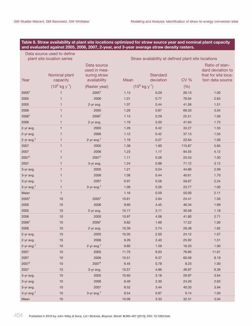
the standard deviation (i.e. decreases in effi ciency) occurred if alternate years were used to defi ne plant locations from those used to measure straw availability around the plants (Table 8). Relative increases in standard deviations were greatest for the 1 million kg y-1 capacity plants (e.g. 2006 straw availability and 2005 plant site locations had a stand-ard deviation 2.6 times as large as that measured with 2005 straw availability). Similarly, 2005 straw availability and 2006 plant site locations had a standard deviation 3.0 times as large as that measured with 2006 straw availability. Site locations based on the third year (2007) had even more dramatic impact on effi ciency of utilizing available straw from 2005 and 2006, with 5.7- and 4.2-fold increases in standard deviations. Th e impact of using one year to defi ne optimal plant site locations and another to measure straw availability decreased with increasing nomimal plant capac-ity. Th e ratios of the standard deviations dropped from 2.6
to 1.7 to 1.1 for siting the 1, 10, and 100 million kg y-1 plants when 2005 sites were based on 2006 availability. Similary, the ratios dropped from 3.0 to 2.7 to 1.5 when 2006 sites were based on 2005 straw availability. In the most extreme case, ratios were 5.6 and 4.1 at 1 million kg y-1 capacity, 11.6 and 8.2 at 10 million kg y-1 capacity, and 5.8 and 3.8 at 100 million kg y-1 capacity for plants sites based on 2007 straw availability and measured with 2005 and 2006 straw.
One approach to minimize year-to-year fl uctations in straw availability within defi ned distances around fi xed plant locations was to use multi-year average straw availability to defi ne plant site locations and straw collection distances. Th e risk to this method was that locations would be less than optimally sited every year. In fact, the standard deviation of straw availability within each year averaged 1.8, 2.3, and 1.2 times that of the best sites for the 1, 10, and 100 million kg capacity plants. Standard deviation of straw
Table 4. Average realized straw availability by state and year for each 10 percentile increment in percentage of total available straw assigned to optimal locations of 100 million kg y-1 nominal capacity straw conversion plants.
Incremental percentiles of total available straw assigned to optimal plant site locations
State Year 10% 20% 30% 40% 50% 60% 70% 80% 90% 100%
Average straw assigned per plant site (1 000 000 kg)Idaho 2005 91.08 93.01 88.94 118.07 136.43 111.06 159.47 166.63 144.57 164.66
Oregon 2005 86.02 118.19 98.89 107.97 120.64 163.57 168.78 127.56 110.20 125.05
Washington 2005 99.79 96.68 95.09 94.46 90.10 102.40 101.78 94.91 169.74 166.10
PNW total 2005 90.85 102.02 93.54 107.00 123.45 116.92 149.70 130.13 137.31 145.09
Idaho 2006 84.06 100.33 112.51 111.87 142.85 119.22 159.69 142.72 105.41 140.83
Oregon 2006 85.46 98.74 95.25 94.83 145.45 176.62 132.40 172.03 132.27 128.47
Washington 2006 97.24 90.55 84.07 80.86 101.94 96.75 99.19 96.28 84.70 120.34
PNW total 2006 87.26 97.08 94.40 101.02 130.08 122.33 136.67 130.01 112.01 129.88
Idaho 2-yr avg. 91.64 90.63 120.55 119.88 137.46 103.39 118.04 160.57 170.70 175.23
Oregon 2-yr avg. 85.87 99.68 104.36 82.58 110.66 128.80 93.20 146.92 121.02 116.18
Washington 2-yr avg. 99.33 96.59 108.56 102.96 104.99 114.43 82.02 99.49 169.02 135.35
PNW total 2-yr avg. 91.00 95.44 111.48 101.58 120.24 113.80 96.61 135.66 150.50 143.63
Idaho 2007 110.30 107.41 93.64 99.79 95.21 105.54 112.31 99.84 82.00 116.86
Oregon 2007 97.18 93.52 96.25 102.78 88.47 99.05 95.18 91.56 85.28 94.34
Washington 2007 99.09 104.06 103.77 101.55 97.12 109.70 104.99 91.68 102.09 101.54
PNW total 2007 100.94 101.66 97.89 101.34 93.60 104.61 102.52 94.36 89.79 102.83
Idaho 3-yr avg. 98.22 97.72 110.35 102.64 102.46 91.17 92.81 100.97 90.48 133.75
Oregon 3-yr avg. 98.32 89.89 99.32 96.80 97.59 88.93 96.37 91.82 102.38 90.99
Washington 3-yr avg. 97.81 100.07 97.43 92.18 110.61 100.94 99.95 97.13 96.78 90.96
PNW total 3-yr avg. 98.18 96.16 103.35 97.15 102.19 93.32 95.78 97.26 95.68 103.20
398 Published in 2010 by John Wiley & Sons, Ltd | Biofuels, Bioprod. Bioref. 4:385–407 (2010); DOI: 10.1002/bbb
GW Mueller-Warrant, GM Banowetz, GW Whittaker Modeling and Analysis: Identification of straw-to-energy conversion sites
availability using the 3-y average for siting plants was lower than for using any single alternate year for siting plants.
Geographical distribution of bioenergy
conversion plants
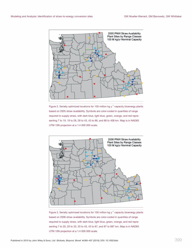
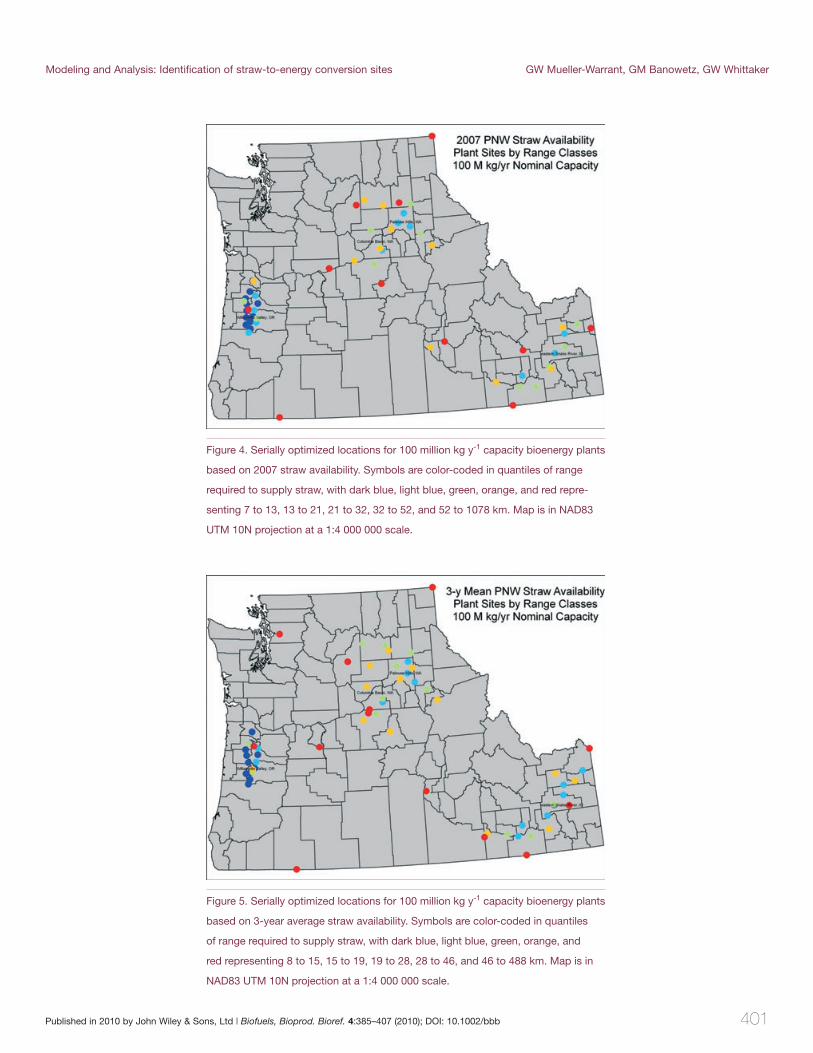
In 2005, the fi rst 20% of the 100 million kg y-1 plants were strongly clustered in three regions, the Willamette Valley in OR, the eastern Snake River Valley in ID, and the Palouse Hills in WA (Fig. 2). Th e next 20% of plants were located in areas adjacent to these clusters or in the Columbia Basin in WA. Th e third and fourth 20% of sites were located at greater distances from the same clusters, while the fi nal 20% were scattered across the rest of the PNW. Generally similar patterns existed in 2006, except for the absence of any of the fi rst 20% of sites in ID (Fig. 3). Plant sites were more strongly clustered in 2007, and all of the fi rst 20% of sites were located in the Willamette Valley in OR (Fig. 4). Even the fi nal 20% of
sites that year were more closely linked to the main clusters than in previous years, with only a few plants falling at loca-tions near edges of the PNW.
Th e 3-year average straw density data for the 100 million kg y-1 capacity plants sited most of the fi rst 20% of plants in the Willamette Valley in OR, with a few in the eastern Snake River Valley in ID (Fig. 5). Th e next 20% were located in the same two regions or the Palouse Hills or Columbia Basin in WA. Th e third 20% were primarily located in WA or the western Snake River Valley in ID. Th e fourth 20% covered a more diff use area in WA with a few plants in ID or western OR. Th e fi nal 20% included some widely scat-tered sites in addition to the clusters present in the earlierly selected sites.
Data for the 10 million kg y-1 capacity plants from the 3-year average straw density identifi ed the Willamette Valley in OR as the primary location for the fi rst 20% of plants, with
Table 5. Average distances (km) required to provide sufficient straw to supply 1 million kg y-1 nominal capacity straw conversion plants by state and year for each 10 percentile increment in total straw assigned to plants.
Incremental percentiles of total available straw assigned to optimal plant site locations
State Year 10% 20% 30% 40% 50% 60% 70% 80% 90% 100%
Average range required for adequate straw to meet plant capacity (km)Idaho 2005 1.1 1.4 1.5 1.7 1.8 2.0 2.2 2.5 3.4 13.9
Oregon 2005 0.9 1.2 1.3 1.5 1.7 1.8 2.0 2.3 3.0 13.0
Washington 2005 1.3 1.5 1.7 1.9 2.1 2.2 2.5 3.0 4.2 15.5
PNW total 2005 1.1 1.3 1.5 1.7 1.8 2.0 2.2 2.6 3.5 14.0
Idaho 2006 1.2 1.5 1.6 1.8 2.0 2.1 2.3 2.8 4.1 32.3
Oregon 2006 0.9 1.1 1.3 1.5 1.7 1.8 2.0 2.3 3.1 15.5
Washington 2006 1.4 1.5 1.7 1.8 2.0 2.2 2.4 3.0 4.8 19.2
PNW total 2006 1.1 1.4 1.6 1.7 1.9 2.1 2.3 2.7 4.0 22.9
Idaho 2-yr avg. 1.2 1.4 1.6 1.7 1.9 2.1 2.3 2.6 4.1 12.4
Oregon 2-yr avg. 0.9 1.2 1.4 1.5 1.7 1.9 2.1 2.3 3.2 11.2
Washington 2-yr avg. 1.4 1.6 1.7 1.9 2.1 2.3 2.6 3.5 5.3 12.5
PNW total 2-yr avg. 1.1 1.4 1.6 1.7 1.9 2.1 2.3 2.8 4.1 12.0
Idaho 2007 1.3 1.6 1.8 1.9 2.1 2.3 2.6 3.5 5.4 31.4
Oregon 2007 0.8 1.1 1.3 1.5 1.7 1.8 2.0 2.3 3.2 17.5
Washington 2007 1.4 1.6 1.8 2.0 2.2 2.3 2.7 3.8 5.6 16.8
PNW total 2007 1.1 1.4 1.6 1.8 2.0 2.1 2.4 3.2 4.6 21.8
Idaho 3-yr avg. 1.2 1.5 1.7 1.8 2.0 2.1 2.3 2.9 4.9 31.2
Oregon 3-yr avg. 0.9 1.2 1.4 1.5 1.7 1.9 2.1 2.4 3.4 19.2
Washington 3-yr avg. 1.5 1.7 1.8 2.0 2.1 2.4 2.8 4.0 5.9 16.6
PNW total 3-yr avg. 1.2 1.4 1.6 1.8 1.9 2.1 2.4 3.0 4.6 23.0
Published in 2010 by John Wiley & Sons, Ltd | Biofuels, Bioprod. Bioref. 4:385–407 (2010); DOI: 10.1002/bbb 399
Modeling and Analysis: Identification of straw-to-energy conversion sites GW Mueller-Warrant, GM Banowetz, GW Whittaker
Figure 2. Serially optimized locations for 100 million kg y-1 capacity bioenergy plants
based on 2005 straw availability. Symbols are color-coded in quantiles of range
required to supply straw, with dark blue, light blue, green, orange, and red repre-
senting 7 to 19, 19 to 28, 28 to 43, 43 to 88, and 88 to 408 km. Map is in NAD83
UTM 10N projection at a 1:4 000 000 scale.
Figure 3. Serially optimized locations for 100 million kg y-1 capacity bioenergy plants
based on 2006 straw availability. Symbols are color-coded in quantiles of range
required to supply straw, with dark blue, light blue, green, orange, and red repre-
senting 7 to 20, 20 to 33, 33 to 43, 43 to 87, and 87 to 687 km. Map is in NAD83
UTM 10N projection at a 1:4 000 000 scale.
400 Published in 2010 by John Wiley & Sons, Ltd | Biofuels, Bioprod. Bioref. 4:385–407 (2010); DOI: 10.1002/bbb
GW Mueller-Warrant, GM Banowetz, GW Whittaker Modeling and Analysis: Identification of straw-to-energy conversion sites
Table 6. Average distances (km) required to provide sufficient straw to supply 10 million kg y-1 nominal capacity straw conversion plants by state and year for each 10 percentile increment in total straw assigned to plants.
Incremental percentiles of total available straw assigned to optimal plant site locations
State Year 10% 20% 30% 40% 50% 60% 70% 80% 90% 100%
Average range required for adequate straw to meet plant capacity (km)Idaho 2005 3.2 3.9 5.0 6.7 8.3 10.6 13.4 18.5 30.6 101.6
Oregon 2005 2.3 2.8 3.5 4.0 5.0 6.6 9.8 13.7 25.5 98.7
Washington 2005 4.1 4.6 6.1 7.4 9.7 12.7 16.6 19.8 25.0 94.3
PNW total 2005 3.1 3.7 4.8 6.0 7.5 9.8 12.9 17.1 27.6 99.0
Idaho 2006 3.6 4.3 5.0 5.6 6.6 7.9 9.7 12.6 19.0 57.5
Oregon 2006 2.3 2.9 3.2 3.7 4.6 5.7 7.7 11.3 16.5 62.1
Washington 2006 4.2 4.7 5.0 5.5 6.1 7.3 8.6 11.3 16.8 59.1
PNW total 2006 3.3 3.9 4.5 4.9 5.8 7.0 8.7 11.8 17.5 59.5
Idaho 2-yr avg. 3.5 4.0 4.5 5.2 5.7 6.5 7.9 10.8 16.0 48.0
Oregon 2-yr avg. 2.4 2.9 3.3 3.7 4.7 5.7 7.6 9.8 15.9 62.1
Washington 2-yr avg. 4.3 4.7 5.2 5.8 6.5 7.6 8.9 12.1 17.4 52.1
PNW total 2-yr avg. 3.3 3.8 4.3 4.8 5.6 6.5 8.1 10.9 16.3 53.6
Idaho 2007 3.9 4.6 5.2 5.9 7.0 8.1 9.6 13.4 19.4 79.7
Oregon 2007 2.2 2.5 2.8 3.3 3.8 4.5 5.5 7.1 12.9 76.6
Washington 2007 4.5 5.0 5.6 6.2 7.0 8.4 9.8 12.1 16.6 40.8
PNW total 2007 3.3 3.9 4.3 4.9 5.7 6.7 8.0 10.4 15.9 68.4
Idaho 3-yr avg. 3.7 4.3 4.8 5.5 6.1 6.9 8.2 11.5 17.6 88.9
Oregon 3-yr avg. 2.3 2.7 3.1 3.5 4.0 4.9 5.8 7.4 11.1 39.6
Washington 3-yr avg. 4.6 5.1 5.5 6.0 6.9 8.2 9.9 12.3 18.0 66.5
PNW total 3-yr avg. 3.5 4.0 4.4 4.9 5.5 6.6 7.7 10.2 15.4 64.9
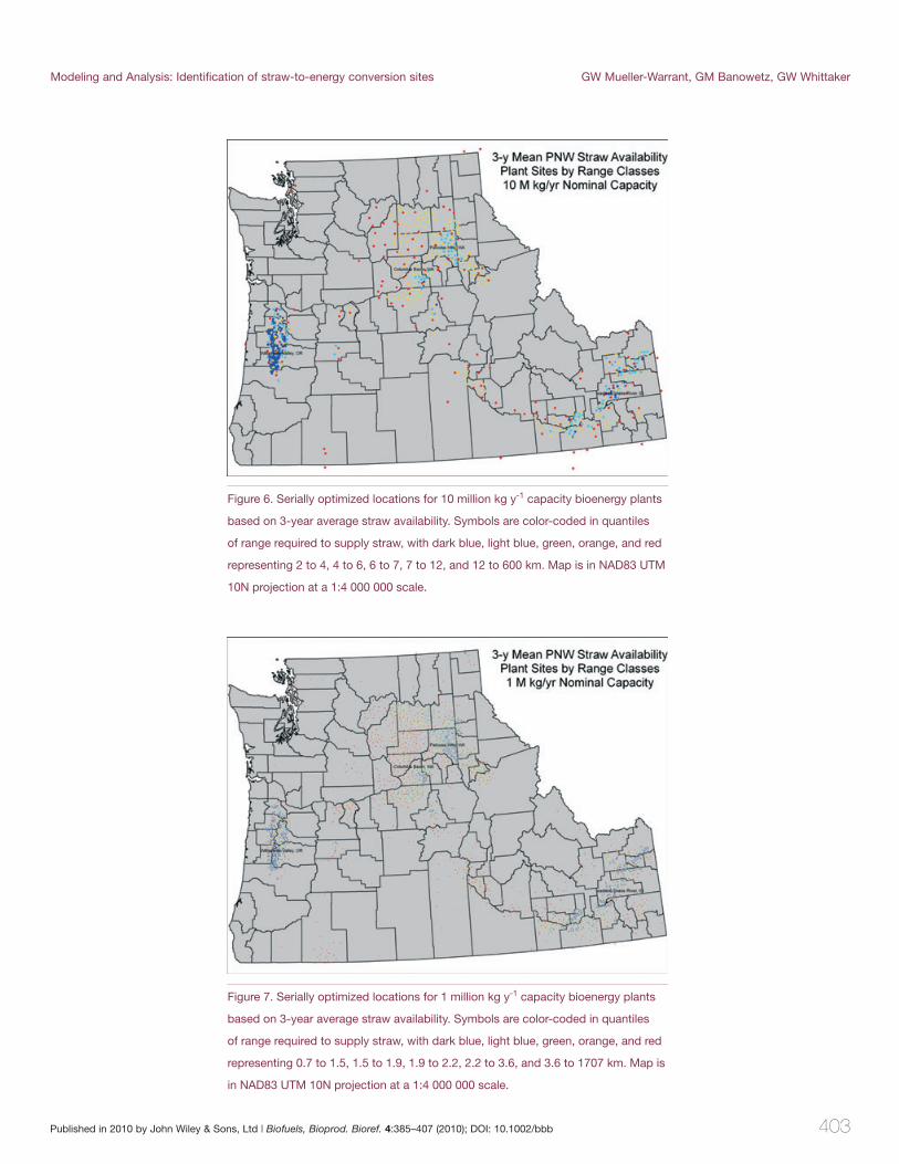
additional plants in the southern and eastern Snake River Valley in ID and LaGrande, OR. (Fig. 6) Th e next 20% of sites covered these same regions plus the Palouse Hills and Columbia Basin in WA and Madras, OR. Th e third 20% was more broadly scattered across eastern WA and the Snake River Valley in ID. Th e fourth 20% mainly covered additional areas in eastern WA. Most of the fi nal 20% surrounded the clusters of the fi rst 80%, with a small number of sites located near edges of the PNW. Siting order patterns for the 1 million kg y-1 capacity plants were more evenly distributed among states and main cluster areas than had been the case for the larger capacity plants, with large numbers of the fi rst 20% of sites present in the Willamette Valley of OR, the Palouse Hills and Columbia Basin in WA, LaGrande, OR, and the eastern Snake River Valley in ID (Fig. 7). Additional clusters appeared in the second, third, and fourth 20% of sites, with the fi nal 20% more diff usely scattered across larger areas.
One obvious implication of patterns at these three plant capacities is that technology for the 1 million kg y-1 plants may well be applicable across broader areas of the PNW than technology for the larger plants, especially if transportation costs are signifi cant fractions of total operating expenses. An example of possible technological diff erences between the 1 million kg y-1 capacity plants and larger ones is the method used to collect straw in the fi eld and transport it to the processing site. Forage choppers, wagons, and silage blowers are already utilized in livestock production on farms operat-ing over ranges of several km out from central farmsteads, and their adoption as a straw handling system for cereal grain and grass seed farming might reduce costs compared to baling, especially for traditional 25 to 40 kg bales handled with sig-nifi cant manual labor. Economics of scale of processes within bioenergy conversion plants will presumably favor relatively large sizes. Reduced distances for transporting straw and the
Published in 2010 by John Wiley & Sons, Ltd | Biofuels, Bioprod. Bioref. 4:385–407 (2010); DOI: 10.1002/bbb 401
Modeling and Analysis: Identification of straw-to-energy conversion sites GW Mueller-Warrant, GM Banowetz, GW Whittaker
Figure 5. Serially optimized locations for 100 million kg y-1 capacity bioenergy plants
based on 3-year average straw availability. Symbols are color-coded in quantiles
of range required to supply straw, with dark blue, light blue, green, orange, and
red representing 8 to 15, 15 to 19, 19 to 28, 28 to 46, and 46 to 488 km. Map is in
NAD83 UTM 10N projection at a 1:4 000 000 scale.
Figure 4. Serially optimized locations for 100 million kg y-1 capacity bioenergy plants
based on 2007 straw availability. Symbols are color-coded in quantiles of range
required to supply straw, with dark blue, light blue, green, orange, and red repre-
senting 7 to 13, 13 to 21, 21 to 32, 32 to 52, and 52 to 1078 km. Map is in NAD83
UTM 10N projection at a 1:4 000 000 scale.
402 Published in 2010 by John Wiley & Sons, Ltd | Biofuels, Bioprod. Bioref. 4:385–407 (2010); DOI: 10.1002/bbb
GW Mueller-Warrant, GM Banowetz, GW Whittaker Modeling and Analysis: Identification of straw-to-energy conversion sites
possible use of alternative straw handling systems may favor the farm-scale bioenergy conversion plants suffi ciently to off -set the advantages of large, centralized plants. Absent market distortions induced by taxation and subsidy policies favor-ing one size plant over another, mixes of large and small size bioenergy conversion plants should co-exist, with lower straw transportation costs in the smaller plants and economies of scale in the larger plants tended to off set one another.
Infrastructure concerns of sites based solely on
maximized neighborhood straw density
Conversion plants sited solely on the basis of minimized transportation distance for straw may be misaligned with critical infrastructure components, such as the electrical power grid, road and railway transportation networks,25 and suitable landuse planning zones. While thorough analysis of these complicating factors is beyond the scope of this manu-script, we did test for alignment of the SSAO sites from the
Table 7. Average distances required to provide sufficient straw to supply 100 million kg y-1 nominal capacity straw conversion plants by state and year for each 10 percentile increment in total straw assigned to plants.
Incremental percentiles of total available straw assigned to optimal plant site locations
State Year 10% 20% 30% 40% 50% 60% 70% 80% 90% 100%
Average range required for adequate straw to meet plant capacity (km)Idaho 2005 13.8 17.6 22.9 29.0 32.4 47.9 72.6 86.1 161.9 259.6
Oregon 2005 7.4 14.2 23.7 28.4 33.3 48.6 69.2 76.7 96.6 279.7
Washington 2005 13.7 14.2 19.3 22.7 25.8 38.3 49.0 66.0 104.1 219.3
PNW total 2005 11.7 15.9 22.1 27.0 31.6 44.8 65.0 76.1 130.5 262.9
Idaho 2006 22.2 33.1 38.9 42.8 54.4 61.8 74.8 82.1 177.7 470.0
Oregon 2006 7.5 11.5 15.9 28.7 40.1 43.2 54.7 131.1 150.4 399.8
Washington 2006 14.4 16.0 18.5 24.1 25.3 28.6 35.9 38.6 86.7 190.3
PNW total 2006 14.8 22.1 20.6 35.0 39.9 40.6 59.0 74.5 148.6 353.4
Idaho 2-yr avg. 16.7 25.0 29.0 39.1 47.0 73.3 88.7 89.9 105.2 200.1
Oregon 2-yr avg. 7.5 11.9 16.7 19.7 24.3 32.1 36.0 62.1 126.9 343.1
Washington 2-yr avg. 14.5 14.7 19.6 24.9 34.0 36.1 42.1 52.8 104.4 234.5
PNW total 2-yr avg. 13.2 17.7 22.0 28.5 35.3 50.9 50.7 68.2 113.7 264.2
Idaho 2007 16.9 17.7 20.3 24.1 26.1 35.4 38.2 44.2 91.0 136.5
Oregon 2007 7.5 8.4 10.0 11.0 12.6 13.2 15.4 23.4 33.0 158.2
Washington 2007 14.9 17.7 21.3 26.4 30.4 35.6 37.5 50.5 87.1 690.8
PNW total 2007 11.7 14.6 17.2 19.3 23.0 26.6 26.7 39.3 70.3 304.2
Idaho 3-yr avg. 14.0 16.4 17.5 18.1 25.3 27.5 29.0 46.3 98.2 276.5
Oregon 3-yr avg. 7.9 9.2 10.7 11.7 13.2 14.8 21.8 28.4 47.0 186.4
Washington 3-yr avg. 14.8 16.2 19.6 20.9 24.7 26.4 32.2 39.5 44.7 296.2
PNW total 3-yr avg. 11.7 14.3 15.2 16.2 21.1 23.6 26.0 39.2 68.3 243.5
2007 straw density data with the electrical power grid (using satellite night light data16 as a proxy) and with the road and railway transportation networks.25 For the 1 million kg y-1 capacity plants, 58% of all sites aligned with electrical power grid proxy to within less than 1 km discrepancy. Of those sites apparently not on the grid, relocation distances of 3, 6, and 9 km would leave only 28, 15, and 8% of sites without pre-existing connections to the electrical grid. Given that the median buff er distance for plants of this size had been only 2.1 km, it is possible that approximately one-third of our proposed locations were suffi ciently far from the electri-cal grid to require potentially expensive additions to pow-erlines or movement of the facilities to less than optimal locations in terms of straw density (defi ning that condition as occurring whenever displacement distance was similar to, or larger in size than, the buff er distance itself).
For the 10 million kg y-1 capacity plants, 60% of all sites aligned with electrical power grid proxy to within less than
Published in 2010 by John Wiley & Sons, Ltd | Biofuels, Bioprod. Bioref. 4:385–407 (2010); DOI: 10.1002/bbb 403
Modeling and Analysis: Identification of straw-to-energy conversion sites GW Mueller-Warrant, GM Banowetz, GW Whittaker
Figure 6. Serially optimized locations for 10 million kg y-1 capacity bioenergy plants
based on 3-year average straw availability. Symbols are color-coded in quantiles
of range required to supply straw, with dark blue, light blue, green, orange, and red
representing 2 to 4, 4 to 6, 6 to 7, 7 to 12, and 12 to 600 km. Map is in NAD83 UTM
10N projection at a 1:4 000 000 scale.
Figure 7. Serially optimized locations for 1 million kg y-1 capacity bioenergy plants
based on 3-year average straw availability. Symbols are color-coded in quantiles
of range required to supply straw, with dark blue, light blue, green, orange, and red
representing 0.7 to 1.5, 1.5 to 1.9, 1.9 to 2.2, 2.2 to 3.6, and 3.6 to 1707 km. Map is
in NAD83 UTM 10N projection at a 1:4 000 000 scale.
404 Published in 2010 by John Wiley & Sons, Ltd | Biofuels, Bioprod. Bioref. 4:385–407 (2010); DOI: 10.1002/bbb
GW Mueller-Warrant, GM Banowetz, GW Whittaker Modeling and Analysis: Identification of straw-to-energy conversion sites
Table 8. Straw availability at plant site locations optimized for straw source year and nominal plant capacity and evaluated against 2005, 2006, 2007, 2-year, and 3-year average straw density rasters.
Data source used to defi ne plant site location series Straw availability at defi ned plant site locations
YearNominal plant
capacity
Data source used in mea-suring straw availability Mean
Standard deviation CV %
Ratio of stan-dard deviation to that for site loca-tion data source
(106 kg y-1) (Raster year) (106 kg y-1) (%)2005† 1 2005† 1.13 0.29 26.13 1.00
2005 1 2006 1.01 0.77 76.94 2.63
2005 1 2-yr avg. 1.07 0.44 41.56 1.51
2006 1 2005 1.26 0.87 69.33 3.04
2006† 1 2006† 1.13 0.29 25.51 1.00
2006 1 2-yr avg. 1.19 0.50 41.64 1.73
2-yr avg. 1 2005 1.26 0.42 33.27 1.55
2-yr avg. 1 2006 1.12 0.42 37.13 1.55
2-yr avg.† 1 2-yr avg.† 1.19 0.27 22.64 1.00
2007 1 2005 1.38 1.60 115.87 5.65
2007 1 2006 1.23 1.17 94.55 4.12
2007† 1 2007† 1.11 0.28 25.53 1.00
2007 1 3-yr avg. 1.24 0.88 71.12 3.12
3-yr avg. 1 2005 1.21 0.54 44.66 2.09
3-yr avg. 1 2006 1.08 0.44 40.61 1.70
3-yr avg. 1 2007 0.97 0.58 59.67 2.24
3-yr avg.† 1 3-yr avg.† 1.09 0.26 23.77 1.00
Mean 1 1.16 0.59 50.00 2.11
2005† 10 2005† 10.81 2.64 24.41 1.00
2005 10 2006 9.60 4.45 46.34 1.69
2005 10 2-yr avg. 10.17 3.11 30.58 1.18
2006 10 2005 10.97 4.58 41.80 2.71
2006† 10 2006† 9.82 1.69 17.22 1.00
2006 10 2-yr avg. 10.39 2.74 26.38 1.62
2-yr avg. 10 2005 10.35 2.50 24.12 1.57
2-yr avg. 10 2006 9.26 2.40 25.92 1.51
2-yr avg.† 10 2-yr avg.† 9.80 1.59 16.20 1.00
2007 10 2005 11.75 9.03 76.85 11.61
2007 10 2006 10.51 6.37 60.56 8.19
2007† 10 2007† 9.45 0.78 8.23 1.00
2007 10 3-yr avg. 10.57 4.96 46.97 6.39
3-yr avg. 10 2005 10.60 3.18 29.97 3.64
3-yr avg. 10 2006 9.49 2.30 24.20 2.63
3-yr avg. 10 2007 8.52 3.44 40.33 3.94
3-yr avg.† 10 3-yr avg.† 9.54 0.87 9.14 1.00
Mean 10 10.09 3.33 32.31 3.04
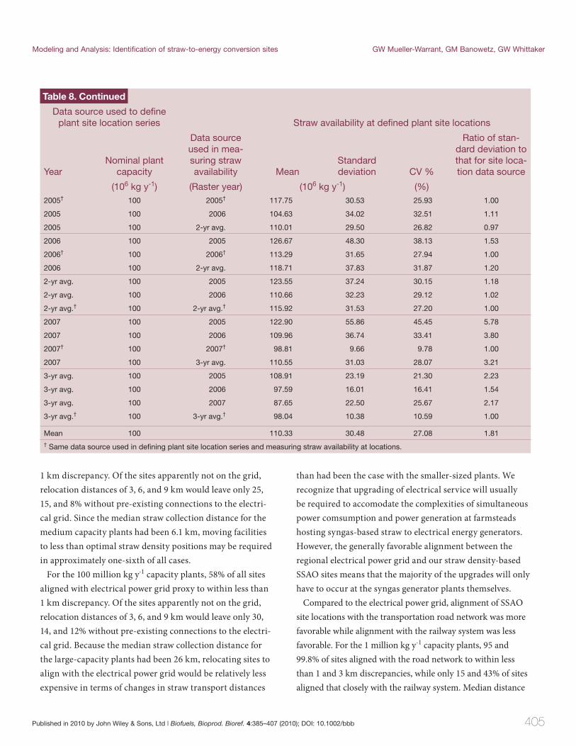
Published in 2010 by John Wiley & Sons, Ltd | Biofuels, Bioprod. Bioref. 4:385–407 (2010); DOI: 10.1002/bbb 405
Modeling and Analysis: Identification of straw-to-energy conversion sites GW Mueller-Warrant, GM Banowetz, GW Whittaker
2005† 100 2005† 117.75 30.53 25.93 1.00
2005 100 2006 104.63 34.02 32.51 1.11
2005 100 2-yr avg. 110.01 29.50 26.82 0.97
2006 100 2005 126.67 48.30 38.13 1.53
2006† 100 2006† 113.29 31.65 27.94 1.00
2006 100 2-yr avg. 118.71 37.83 31.87 1.20
2-yr avg. 100 2005 123.55 37.24 30.15 1.18
2-yr avg. 100 2006 110.66 32.23 29.12 1.02
2-yr avg.† 100 2-yr avg.† 115.92 31.53 27.20 1.00
2007 100 2005 122.90 55.86 45.45 5.78
2007 100 2006 109.96 36.74 33.41 3.80
2007† 100 2007† 98.81 9.66 9.78 1.00
2007 100 3-yr avg. 110.55 31.03 28.07 3.21
3-yr avg. 100 2005 108.91 23.19 21.30 2.23
3-yr avg. 100 2006 97.59 16.01 16.41 1.54
3-yr avg. 100 2007 87.65 22.50 25.67 2.17
3-yr avg.† 100 3-yr avg.† 98.04 10.38 10.59 1.00
Mean 100 110.33 30.48 27.08 1.81† Same data source used in defi ning plant site location series and measuring straw availability at locations.
Table 8. Continued
Data source used to defi ne plant site location series Straw availability at defi ned plant site locations
YearNominal plant
capacity
Data source used in mea-suring straw availability Mean
Standard deviation CV %
Ratio of stan-dard deviation to that for site loca-tion data source
(106 kg y-1) (Raster year) (106 kg y-1) (%)
1 km discrepancy. Of the sites apparently not on the grid, relocation distances of 3, 6, and 9 km would leave only 25, 15, and 8% without pre-existing connections to the electri-cal grid. Since the median straw collection distance for the medium capacity plants had been 6.1 km, moving facilities to less than optimal straw density positions may be required in approximately one-sixth of all cases.
For the 100 million kg y-1 capacity plants, 58% of all sites aligned with electrical power grid proxy to within less than 1 km discrepancy. Of the sites apparently not on the grid, relocation distances of 3, 6, and 9 km would leave only 30, 14, and 12% without pre-existing connections to the electri-cal grid. Because the median straw collection distance for the large-capacity plants had been 26 km, relocating sites to align with the electrical power grid would be relatively less expensive in terms of changes in straw transport distances
than had been the case with the smaller-sized plants. We recognize that upgrading of electrical service will usually be required to accomodate the complexities of simultaneous power comsumption and power generation at farmsteads hosting syngas-based straw to electrical energy generators. However, the generally favorable alignment between the regional electrical power grid and our straw density-based SSAO sites means that the majority of the upgrades will only have to occur at the syngas generator plants themselves.
Compared to the electrical power grid, alignment of SSAO site locations with the transportation road network was more favorable while alignment with the railway system was less favorable. For the 1 million kg y-1 capacity plants, 95 and 99.8% of sites aligned with the road network to within less than 1 and 3 km discrepancies, while only 15 and 43% of sites aligned that closely with the railway system. Median distance
406 Published in 2010 by John Wiley & Sons, Ltd | Biofuels, Bioprod. Bioref. 4:385–407 (2010); DOI: 10.1002/bbb
GW Mueller-Warrant, GM Banowetz, GW Whittaker Modeling and Analysis: Identification of straw-to-energy conversion sites
for misalignment with the railway system was 3.5 km, and dis-tance for 11% of sites exceeded 12 km. For the 10 million kg y-1 capacity plants, 94 and 99.3% of sites aligned with the road network to within less than 1 and 3 km discrepancies, while only 15 and 44% of sites aligned that closely with the railway system. Median distance for misalignment with the rail-way system was 3.5 km, and distance for nearly 10% of sites exceeded 12 km. For the 100 million kg y-1 capacity plants, 82 and 96.5% of sites aligned with the road network to within less than 1 and 3 km discrepancies, while only 26 and 47% of sites aligned that closely with the railway system. Median distance for misalignment with the railway system was 3.2 km, and dis-tance for more than 12% of sites exceeded 12 km.
In general, the transportation road network will impose very few direct restrictions on the ability to locate straw to conversion plants at positions minimizing local straw trans-portation distance/cost. While this conclusion is generally independent of plant capacity, concentrated truck traffi c around the largest capacity plants may impose limits on where they can be built without unacceptable interference with other users of the same roads. Th e possibility of using the existing railway system for energy-effi cient transport of intermediate products such as pyrolysis oil from a distrib-uted system of 10 to 100 million kg y-1 capacity plants to one or more centralized refi neries7 may force some of those distributed plants to be sited at non-optimal positions in terms of local straw density. One option to reduce the mis-alignment with the railway network would be to increase the capacity of some of the plants to handle the available straw in their general vicinity, even though this will lead to greater variation in straw density/transportation costs among the plants. Another option would simply be to truck the con-densed liquid from sites off the railway network to collection points on the railway network.
Siting of plants with a mixture of capacities at optimal loca-tions could be accomplished through a relatively straight-forward extension of SSAO that included mechanisms to defi ne the conditions under which capacity of individual plants was increased by some (possibly integer) multiple of the nominal capacity. A prime candidate for such conditions might be failure of N by N neighborhood maxima to align with one or more critical infrastructure components. Moving the proposed plant site to the nearest location possessing the needed infrastructure would inherently increase the buff er
distance to the sum of the original buff er distance plus the spacing between the two locations. Quantity of straw within this larger buff er distance from the new center would likely be considerably more than the nominal plant capacity, and could serve as the basis for selecting a temporarily larger plant capacity. A complication that would occur in the pro-posed siting process would be whether to create a single new plant with larger capacity at the location or create a series of additional plants with the same capacity at all locations hav-ing higher N by N neighborhood average straw density. As an alternative approach, points from an initial SSAO that failed to align with infrastructure components could be moved to the nearest positions with satisfactory infrastructure, and K-means analysis run limiting the allowed relocation posi-tions for facility sites to those with satisfactory infrastructure. As K-means approached stability, sites with less than desired minimum quantities of straw could be dropped one at a time from consideration. Other elaborate combinations of SSAO and K-means could be tested to reduce the number of fi elds that had been eff ectively orphaned by SSAO while retaining its two main strengths: (1) the close coupling between nomi-mal plant capacity and straw assignment; and (2) the low-est-hanging-fruit approach for ranking of sites by local straw density/minimized transportation costs.
Conclusions
Farm-scale bioenergy conversion plants can be sited within several km of adequate straw supplies, providing them with twin advantages of shorter transport distance and greater fl exibility in transport method than the larger capacity, more centralized plants typically considered in previous analyses. Farm-scale plants may be more readily adopted than larger ones because locations with similar straw avail-ability (i.e. distance needed to obtain required quantities of straw) are more evenly distributed across all major regions of cereal and grass seed production in the PNW. Optimally sited plants should experience no more than 2-fold increases in distances required to obtain adequate quantities of straw from the very fi rst plants built on out to the far greater num-bers necessary to process 60 to 70% of total available straw. Spatial variation in straw distribution will likely limit total saturation of the future straw-to-energy conversion industry to no more than 80 to 90% of the total available straw.
Published in 2010 by John Wiley & Sons, Ltd | Biofuels, Bioprod. Bioref. 4:385–407 (2010); DOI: 10.1002/bbb 407
Modeling and Analysis: Identification of straw-to-energy conversion sites GW Mueller-Warrant, GM Banowetz, GW Whittaker
References 1. Banowetz GM, Boaetng A, Steiner JJ, Griffi th SM, Sethi V and
El-Nashaar HM, Assessment of straw biomass feedstock resources in
the Pacifi c Northwest. Biomass Bioenerg 32:629–634 (2008).
2. Graf A and Koehler T, Oregon cellulose-ethanol study: an evaluation of
the potential for ethanol production in Oregon using cellulose-based
feedstocks. Oregon Offi ce of Energy Special Publication, 36 p, (2005).
Available at: http://www.ecy.wa.gov/pubs/0507047.pdf
3. Kerstetter JD and Lyons JK, Logging and agricultural residue supply
curves for the Pacifi c Northwest. Washington State University Energy
Publication (2001).
4. Frear C, Zhao B, Fu G, Richardson M, Chen S and Fuchs MR, An
evaluation of organic material resources for bioenergy production in
Washington State. Publication No. 05-07-047, 124 p. Available, at
http://pacifi cbiomass.org/documents/WA_BioenergyInventoryAnd
Assessment_200512.pdf [October 16, 2009].”
5. Mackey JE, Opportunities in grass straw utilization. Prepared for the
Oregon Economic Development Department and Oregon Department of
Agriculture by CH2M Hill (1991).
6. Boateng AA, Banowetz GM, Steiner JJ, Barton TF, Taylor DG, Hicks KB
et al., Gasifi cation of Kentucky bluegrass (Poa pratensis L.) straw in a
farm scale reactor. Biomass Bioenerg 31:153–161 (2007).
7. Wright MM, Brown RC and Boateng AA, Distributed processing of bio-
mass to bio-oil for subsequent production of Fischer-Tropsch liquids.
Biofuels Bioprod Bioref 2:229–238 (2008).
8. Henrich E, Dahmen N and Dinjus E, Cost estimate for biosynfuel pro duction
via biosyncrude gasifi cation. Biofuels Bioprod Bioref 3:28–41 (2009).
9 Wright M and Brown RC, Establishing the optimal sizes of different kinds
of biorefi neries. Biofuels Bioprod Bioref 1:191–200 (2007).
10, Estivill-Castro V and Houle ME, Robust distance-based clustering with
applications to spatial data mining. Algorithmica 30:216–242 (2001).
11. Jain AK, Murty MN and Flynn PJ, Data clustering: A review. ACM
Computing Surveys 31:264–323 (1999).
12. Zarzani A, Rahgozar M, Lucas C and Taghiyareh F, Spatial data mining
for optimized selection of facility locations in fi eld-based services.
Compu tational Intelligence and Data Mining IEEE Symposium 734–741
(2007).
13. Zarnani A, Rahgozar M, Lucas C and Taghiyareh F, Effective spatial clus-
tering methods for optimal facility establishment. Intelligent Data Analysis
13:61–84 (2009).
14. Likas A, Vlassis V and Verbeek J, The global K-means clustering algo-
rithm. Pattern Recognition 36:451–461 (2003).
15. Matisziw TC and Murray AT, Area coverage maximization in service facil-
ity siting. J. Geogr Syst 11:175–189 (2009).
16. National Geophysical Data Center NOAA Satellite and Information
Service, Version 4 DMSP-OLS Nighttime Lights Time Series. Available
at: http://www.ngdc.noaa.gov/dmsp/downloadV4composites.html
[February 19, 2010].
17. Ragauskas AJ, Williams CK, Davison BH, Britovsek G, Cairney J et al.
The path forward for biofuels and biomaterials. Science 311:484–489
(2006).
18. Kim H, Kim S and Dale BE, Biofuels, land use change, and greenhouse
gas emissions: Some unexplored variables. Environ Sci Technol
43:961–967 (2009).
19. Melillo JM, Reilly JM, Kicklighter DW, Gurgel AC, Cronin TW et al., Indi-
rect emissions from biofuels: How important. Science 326:1397–1399
(2009).
20. USDA-Natural Resources Conservation Service, RUSLE2 Soil Erosion
Prediction Tool, version 1.26.6.4. Available at: http://fargo.nserl.purdue.
edu/rusle2_dataweb/ [August 26, 2008].
21. Geospatial Data Gateway, NASS Cropland Data Layers. Available at:
http://datagateway.nrcs.usda.gov/ [August 27, 2008].
22. NASA Land Processes Distributed Active Archive Center (LP-DAAC),
Available at: https://lpdaac.usgs.gov/ [June 5, 2009].
23. Mueller-Warrant G, Whittaker G, Griffi th S, Banowetz G, Dugger B, Garcia
T et al., Remote sensing classifi cation of grass seed cropping practices
in western Oregon. International J Remote Sensing (2010). In press.
24. Homer C, Yuang C, Limin Y, Wylie B and Coan M, Development of a 2001
national land cover database for the United States. Photogrammetric
Engineering and Remote Sensing 70:829–840 (2004).
25. ArcGIS Desktop version 9.3, Environmental Systems Research Institute
(ESRI), 380 New York Street, Redlands, California 92373–8100. Available
at: http://www.esri.com (January 12, 2009).
George Mueller-Warrant
George Mueller-Warrant has been a Research
Agronomist with the USDA-Agriculture
Research Service (ARS) National Forage
Seed Production Research Center in Corval-
lis, Oregon, since 1985. His research interests
include grass seed production, weed control,
and GIS. He received his MS and PhD
degrees from the University of New Hampshire.
Gary Banowetz
Gary Banowetz is Research Leader of the
USDA-ARS in Corvallis, Oregon. Dr Banowetz
and collaborators are evaluating the feasibility
of using distributed networks of small-scale
technologies to convert straw and other agri-
cultural residues into bioenergy products.
Gerald Whittaker
Gerald Whittaker has been a Research
Hydrologist with the USDA-ARS in Corval-
lis, Oregon, since 1999. Before that, he was
an Economist with the USDA-Economic
Research Service. He received a JD from
Lewis and Clark Law School and an MS from
Oregon State University.