Assessing OpenGL for 2D rendering of geospatial data

- i -

Assessing OpenGL for 2D rendering of geospatial

data

by

Jared Neil Jacobson

12383806

Submitted in partial fulfilment of the requirements for the degree

MSC GEOINFORMATICS

in the

FACULTY OF NATURAL AND AGRICULTURAL SCIENCES

at the

University of Pretoria

SUPERVISOR: S. Coetzee - Department of Geography, Geoinformatics and Meteorology

CO-SUPERVISOR: D.G. Kourie - Department of Computer Science

31 October 2014

- ii -

DECLARATION

I Jared Neil Jacobson declare that the dissertation, which I hereby submit for the degree MSc

Geoinformatics at the University of Pretoria, is my own work and has not previously been submitted by me

for a degree at this or any other tertiary institution.

SIGNATURE_______________________

DATE_____________________________

- iii -

ACKNOWLEDGEMENTS

I wish to extend my sincere gratitude to the following people and institutions for their contributions to this dissertation:

• My supervisor, Professor Serena Coetzee and co-supervisor, Professor Derrick Kourie for their assistance, guidance and encouragement throughout the study;

• My family and friends for their faith in my abilities, continuous support and encouragement throughout the study;

• The University of Pretoria for affording me the opportunity to study at their institution.

- iv -

TABLE OF CONTENTS

DECLARATION .......................................................................................................................................... II

ACKNOWLEDGEMENTS ....................................................................................................................... III

1 INTRODUCTION ................................................................................................................................. 2

1.1 GRAPHIC APIS ............................................................................................................................ 3

1.2 RENDERING ................................................................................................................................ 5

1.3 STATUS QUO: 2D VS. 3D RENDERING OF GEOGRAPHIC DATA ....................................... 7

1.4 RESEARCH MOTIVATION ......................................................................................................... 8

1.5 DISSERTATION OUTLINE ....................................................................................................... 10

2 CPU VS GPU ....................................................................................................................................... 11

2.1 THE CPU AND GPU DATA PROCESSING MODEL ................................................................ 11

2.2 SOFTWARE BASED RENDERING .......................................................................................... 13

2.3 HARDWARE BASED RENDERING ........................................................................................ 15

3 GEOGRAPHIC INFORMATION SYSTEMS .................................................................................... 17

3.1 COMPONENTS OF A GIS ......................................................................................................... 18

3.1.1 Hardware ............................................................................................................................. 18

3.1.2 Software ............................................................................................................................... 24

3.1.3 Data ...................................................................................................................................... 25

3.1.4 People .................................................................................................................................. 28

3.1.5 Methods ............................................................................................................................... 28

3.2 FUNCTIONS OF A GIS .............................................................................................................. 29

3.2.1 Data Collection .................................................................................................................... 29

3.2.2 Data Storage ........................................................................................................................ 30

3.2.3 Manipulation ........................................................................................................................ 31

- v -

3.2.4 Analysis ............................................................................................................................... 32

3.2.5 Data Presentation ................................................................................................................. 33

4 COORDINATE REFERENCE SYSTEMS ......................................................................................... 34

4.1 COORDINATE REFERENCE SYSTEM TYPES ...................................................................... 35

4.2 GEOGRAPHIC COORDINATE SYSTEMS .............................................................................. 36

4.2.1 Spheroids and Spheres ......................................................................................................... 36

4.2.2 The Shape of the Earth ........................................................................................................ 36

4.2.3 Datums ................................................................................................................................. 37

4.3 PROJECTED COORDINATE SYSTEMS.................................................................................. 38

4.4 WHAT IS A MAP PROJECTION? ............................................................................................. 39

4.5 PROJECTION TYPES ................................................................................................................ 40

4.5.1 Conic Projections ................................................................................................................. 41

4.5.2 Cylindrical Projections ........................................................................................................ 42

4.5.3 Planar Projections ................................................................................................................ 42

4.6 PROJECTION PARAMETERS .................................................................................................. 43

4.7 GEOGRAPHIC TRANSFORMATION ...................................................................................... 44

5 OPENGL ............................................................................................................................................. 45

5.1 HARDWARE STACK FOR OPENGL ....................................................................................... 47

5.1.1 System Memory ................................................................................................................... 47

5.2 GRAPHICS TERMINOLOGY ................................................................................................... 48

5.3 GL STATE ................................................................................................................................... 50

5.4 CONTEXT CREATION .............................................................................................................. 52

5.5 DRAWING TO A WINDOW OR VIEW .................................................................................... 52

5.6 DRAWING WITH OPENTK ...................................................................................................... 53

5.7 VIEWING IN OPENGL .............................................................................................................. 66

6 BENCHMARKING ............................................................................................................................ 69

6.1 INTRODUCTION ....................................................................................................................... 69

6.2 DISK BENCHMARKING .......................................................................................................... 70

6.2.1 Results ................................................................................................................................. 72

- vi -

6.3 A SHORT SURVEY INTO EXISTING WINDOWS BASED GRAPHIC APIS ........................ 74

6.3.1 GDI ...................................................................................................................................... 74

6.3.2 GDI+ .................................................................................................................................... 76

6.3.3 Direct2D .............................................................................................................................. 76

6.3.4 DirectX ................................................................................................................................ 76

6.3.5 OpenGL ............................................................................................................................... 77

6.4 IMPLEMENTING A BENCHMARKING APPLICATION ....................................................... 77

6.5 BENCHMARK APPLICATION DESIGN.................................................................................. 80

6.5.1 ILayer Interface ................................................................................................................... 81

6.5.2 Using the API benchmark application ................................................................................. 84

6.6 RESULTS .................................................................................................................................... 85

6.6.1 GDI API ............................................................................................................................... 86

6.6.2 GDI+ API ............................................................................................................................. 87

6.6.3 DirectX API ......................................................................................................................... 88

6.6.4 OpenGL API ........................................................................................................................ 89

6.6.5 Direct 2D API ...................................................................................................................... 90

6.7 CONCLUSION ........................................................................................................................... 91

7 RESEARCH EXPERIMENT .............................................................................................................. 93

7.1 INTRODUCTION ....................................................................................................................... 93

7.2 METHOD .................................................................................................................................... 94

7.3 IMPLEMENTING A BASIC GIS VIEWER IN OPENGL ......................................................... 94

7.4 DATA STORAGE ........................................................................................................................ 94

7.5 CODE IN MORE DETAIL ......................................................................................................... 97

7.5.1 Getting data from SpatiaLite ............................................................................................... 97

7.5.2 Building a VBO and drawing an image ............................................................................... 99

7.5.3 High level architecture ....................................................................................................... 102

7.6 SUMMARY ............................................................................................................................... 103

8 GENERAL-PURPOSE COMPUTING ON THE GPU - USING OPENGL/OPENCL INTEROPT FOR

RENDERING TOPOJSON ........................................................................................................................... 105

8.1 INTRODUCTION ..................................................................................................................... 105

- vii -

8.2 THE EVOLUTION OF JSON IN GIS ...................................................................................... 106

8.2.1 JSON .................................................................................................................................. 106

8.2.2 The GeoJSON format ........................................................................................................ 107

8.2.3 TopoJSON ......................................................................................................................... 109

8.2.4 GeoJSON vs TopoJSON ..................................................................................................... 110

8.2.5 Interpreting the TopoJSON Format .................................................................................... 111

8.3 METHOD ................................................................................................................................... 112

8.3.1 Step 1: Creating a TopoJSON file....................................................................................... 112

8.3.2 Step 2: Creating a TopoJSON file reader ............................................................................ 112

8.3.3 Step 3: Drawing a TopoJSON file via OpenGL ................................................................. 114

8.3.4 Step 4: Sending data to an OpenCL kernel ......................................................................... 115

8.4 RESULTS .................................................................................................................................. 120

9 CONCLUSION AND CLOSING REMARKS ................................................................................. 121

10 REFERENCES AND BIBLIOGRAPHY ...................................................................................... 122

11 APPENDIX A - SOURCE CODE AND PROJECT INFORMATION ......................................... 127

11.1 API BENCHMARKING APPLICATION ............................................................................. 127

11.1.1 GUI.BenchmarkingApp ..................................................................................................... 128

11.1.2 Console Application Benchmarks - ADO.NET SQLite Benchmark ................................. 129

11.1.3 Console Application Benchmarks - ADO.NET SQLite Benchmark using custom ADO.NET

wrapper 130

11.1.4 Console Application Benchmarks - ADO.NET SQLite Benchmark using ADO.NET and a

.NET list 130

11.1.5 Console Application Benchmarks - ADO.NET SQLite Benchmark using ADO.NET and a

.NET list 130

11.1.6 Summary ............................................................................................................................ 131

11.2 NETGIS - POINTS OF INTEREST RENDERING APPLICATION WITH ZOOM AND PAN

131

11.3 TOPOJSON - RENDERING USING OPENGL/OPENCL .................................................. 132

- viii -

LIST OF FIGURES

Figure 1 - Differences in GPU and CPU hardware architectures (Das, 2011) ................................................ 12

Figure 2 - General Graphics software pipeline (Mileff & Dudra, 2012) ......................................................... 14

Figure 3 - Components of a GIS ...................................................................................................................... 18

Figure 4 - Intel Q67 Chipset (Intel, 2010) ....................................................................................................... 19

Figure 5 - Diagrammatic representation of a HDD (Cady, Zhuang, & Harchol-Balter, 2011) ........................ 20

Figure 6 - Most popular RAID configurations (Leurs, 2014) ......................................................................... 21

Figure 7 - Dell Precision M4600 memory values ............................................................................................ 23

Figure 8 - GIS layers overlaid to produce a final map image (United States Geological Survey, 2014) ........ 25

Figure 9 - GIS Data Models (Neteler & Mitasova, 2008) ............................................................................... 26

Figure 10 - Data dimensions in a GIS (Neteler & Mitasova, 2008) ................................................................ 27

Figure 11 - Differences in data dimensionality ............................................................................................... 28

Figure 12 - The data collection process ........................................................................................................... 29

Figure 13 - Geometric transformation (Schmandt, 2014) ............................................................................... 32

Figure 14 - Area by industry class ................................................................................................................... 33

Figure 15 - Surface of the earth (OGP, 2008) .................................................................................................. 34

Figure 16 - Difference between a sphere and spheroid (ESRI, 2004) ............................................................. 36

Figure 17 - Major and minor axes of an ellipse (ESRI, 2004) ........................................................................ 37

Figure 18 - Error caused by using the wrong datum (Egbert & Dunbar, 2007) .............................................. 38

Figure 19 - The four quadrants showing positive and negative x and y values (ESRI, 2004)......................... 38

Figure 20 - The graticule of a geographic coordinate system is projected onto a cylindrical projection surface

(ESRI, 2004) ............................................................................................................................... 39

Figure 21 - Why distortion happens when coordinates are transformed (ESRI, 2004) ................................... 40

Figure 22 - Conic Projections (ESRI, 2004) .................................................................................................... 41

Figure 23 - Cylindrical Projections defined by alignment of the central axis orientation to the globe (ESRI,

2004) ........................................................................................................................................... 42

Figure 24 - Planar Projections (ESRI, 2004) ................................................................................................... 42

Figure 25 - Planar Projections from different points of view (ESRI, 2004) .................................................... 43

Figure 26 - Data flow through OpenGL (Apple, 2013). .................................................................................. 49

- ix -

Figure 27 - A virtual screen (Apple, 2013) ...................................................................................................... 50

Figure 28 - High level OpenGL breakdown (Apple, 2013) ............................................................................. 51

Figure 29 - Graphics platform model (Apple, 2013) ....................................................................................... 52

Figure 30 - OpenGL primitives (OpenTK, 2014) ............................................................................................ 56

Figure 31 - OpenGL with OpenTK a first example ......................................................................................... 62

Figure 32 - Execution timing result of Figure 31 ............................................................................................ 62

Figure 33 - Identity Matrix .............................................................................................................................. 63

Figure 34 Perspective and orthographic projection ......................................................................................... 64

Figure 35 - Steps in configuring and positioning the viewing frustum (Shreiner, Sellers, Kessenich, & Licea-

Kane, 2013, p207) ....................................................................................................................... 66

Figure 36 - ModelView Matrix (Ahn, 2013) ................................................................................................... 68

Figure 37 - ATTO Benchmark Settings ........................................................................................................... 70

Figure 38 - Read/Write Speeds for PC I/O benchmark ................................................................................... 72

Figure 39 - Read/Write Speeds for Laptop I/O benchmark ............................................................................. 72

Figure 40 - Graphic Outlay of WindowsXP (Walbourn, 2009) ....................................................................... 75

Figure 41 - Graphic Outlay of Windows Vista and Windows 7 (Walbourn, 2009) ......................................... 75

Figure 42 - Rendering distortion ..................................................................................................................... 78

Figure 43 - ILayer interface ............................................................................................................................. 81

Figure 44 - IMap interface ............................................................................................................................... 82

Figure 45 - IRenderer interface ....................................................................................................................... 83

Figure 46 - Benchmark Tool UI ....................................................................................................................... 84

Figure 47 - Benchmark results template .......................................................................................................... 85

Figure 48 - Points Rendering Comparison ...................................................................................................... 86

Figure 49 - Text Rendering Comparison ......................................................................................................... 86

Figure 50 - Lines Rendering Comparison ....................................................................................................... 86

Figure 51 - Polygons Rendering Comparison ................................................................................................. 86

Figure 52 - spatialite_gui application .............................................................................................................. 95

Figure 53 - SpatiaLite import options .............................................................................................................. 96

Figure 54 - Select statement result .................................................................................................................. 96

Figure 55 - GetData() Function Code ............................................................................................................. 98

- x -

Figure 56 - Setup a VBO and draw ................................................................................................................. 99

Figure 57 - Resulting image of the point VBO .............................................................................................. 101

Figure 58 - High level system architecture .................................................................................................... 102

Figure 59 - An example JSON schema definition (Internet Engineering Task Force, 2012) ........................ 106

Figure 60 - A GeoJSON feature collection example ..................................................................................... 108

Figure 61 - Example of specifying a GeoJSON coordinate system .............................................................. 109

Figure 62 - Another GeoJSON example ......................................................................................................... 110

Figure 63 - Another TopoJSON example ....................................................................................................... 110

Figure 64 - TopoJSON Transform .................................................................................................................. 111

Figure 65 - TopoJSON file reader diagram .................................................................................................... 113

Figure 66 - Uploading data to OpenCL .......................................................................................................... 118

Figure 67 - Disable LoaderLock Exception .................................................................................................. 128

Figure 68 - Gui.BenchmarkingApp Main Form ............................................................................................ 129

Figure 69 - NetGIS Application..................................................................................................................... 131

Figure 70 - TopoJSON Application ............................................................................................................... 133

- xi -

LIST OF TABLES

Table 1 - Specifications of test computers ....................................................................................................... 71

Table 2 - Test Data Composition ..................................................................................................................... 77

Table 3 - Hardware specification of graphic benchmark PC's ......................................................................... 79

Table 4 - GDI benchmark results ..................................................................................................................... 87

Table 5 - GDI+ benchmark results .................................................................................................................. 88

Table 6 - DirectX benchmark results ............................................................................................................... 89

Table 7 - OpenGL benchmark results .............................................................................................................. 90

Table 8 - Direct2D benchmark results ............................................................................................................. 91

- 1 -

ABSTRACT

The purpose of this study was to investigate the suitability of using the OpenGL and OpenCL graphics

application programming interfaces (APIs), to increase the speed at which 2D vector geographic information

could be rendered. The research focused on rendering APIs available to the Windows operating system.

In order to determine the suitability of OpenGL for efficiently rendering geographic data, this dissertation

looked at how software and hardware based rendering performed. The results were then compared to that of

the different rendering APIs. In order to collect the data necessary to achieve this; an in-depth study of

geographic information systems (GIS), geographic coordinate systems, OpenGL and OpenCL was conducted.

A simplistic 2D geographic rendering engine was then constructed using a number of graphic APIs which

included GDI, GDI+, DirectX, OpenGL and the Direct2D API. The purpose of the developed rendering engine

was to provide a tool on which to perform a number of rendering experiments. A large dataset was then

rendered via each of the implementations. The processing times as well as image quality were recorded and

analysed. This research investigated the potential issues such as acquiring data to be rendered for the API as

fast as possible. This was needed to ensure saturation at the API level. Other aspects such as difficulty of

implementation as well as implementation differences were examined.

Additionally, leveraging the OpenCL API in conjunction with the TopoJSON storage format as a means of data

compression was investigated. Compression is beneficial in that to get optimal rendering performance from

OpenGL, the graphic data to be rendered needs to reside in the graphics processing unit (GPU) memory bank.

More data in GPU memory in turn theoretically provides faster rendering times. The aim was to utilise the

extra processing power of the GPU to decode the data and then pass it to the OpenGL API for rendering and

display. This was achievable via OpenGL/OpenCL context sharing.

The results of the research showed that on average, the OpenGL API provided a significant speedup of between

nine and fifteen times that of GDI and GDI+. This means a faster and more performant rendering engine could

be built with OpenGL at its core. Additional experiments show that the OpenGL API performed faster than

GDI and GDI+ even when a dedicated graphics device is not present. A challenge early in the experiments was

related to the supply of data to the graphic API. Disk access is orders of magnitude slower than the rest of the

computer system. As such, in order to saturate the different graphics APIs, data had to be loaded into main

memory.

Using the TopoJSON storage format yielded decent data compression allowing a larger amount of data to be

stored on the GPU. However, in an initial experiment, it took longer to process the TopoJSON file into a flat

structure that could be utilised by OpenGL than to simply use the actual created objects, process them on the

central processing unit (CPU) and then upload them directly to OpenGL. It is left as future work to develop a

more efficient algorithm for converting from TopoJSON format to a format that OpenCL can utilise.

- 2 -

1 INTRODUCTION

Computer graphics have come a long way since their inception in the 1960s. A graphics card has become a

standard hardware device in the modern day computer. In order to make use of the hardware acceleration

provided by such cards, it is necessary to utilise supporting graphics libraries that expose the necessary

functionality. When looking at many of the 2D GIS packages available on the Windows platform, an interesting

observation can be made. Most, if not all, use software-based rendering via the CPU for graphics computations.

This means that the graphics hardware, implicitly designed for the purpose of rendering graphics is not being

utilised.

Hardware acceleration could potentially benefit a GIS by providing faster 2D rendering of maps. Traditionally,

graphics cards are utilised for the acceleration of 3D images. They can however provide significant speed up

for 2D graphics as well. By using the graphic processor to perform the map rendering, a faster more efficient

map rendering engine could emerge. Due to the substantial size of many geographic datasets this could lead to

significant time savings and improve the overall user experience when working with these datasets. An

example of a large dataset is a shapefile representing over a million erven across South Africa. This dataset is

over 350MB in size and does not include any attribute data except a numerical key value. This might not sound

like a lot at first, but it requires substantial processing power to turn that data into a rendered image. Raster

datasets can be several times larger, often exceeding sizes of several terabytes.

In this dissertation we will focus on three main graphic APIs which are predominately used in GIS applications

running on the Windows platform: GDI, GDI+ and OpenGL. This conclusion was drawn after reviewing a

number of the open source GIS software available as well as some of the proprietry software like ArcMap.

Walbourn (2009), notes that the primary 2D graphic API since early days has been that of GDI with the newer

version being GDI+. This further strengthens the observation made. This holds true even for many of the latest

applications today. GDI and GDI+ can be considered older APIs as Microsoft does provide higher performant

APIs that do support graphics cards. Even so, the new APIs are still absent in the GIS software investigated.

Conversely in terms of 2D there are virtually no implementations to be found that focus on the rendering of

2D geographic data via the use of graphics hardware at the time of writing.

Building a rendering engine based on an API such as OpenGL that can make use of a GPU would greatly

improve the rendering speed of a 2D GIS system.

Furthermore, moving GIS rendering over to OpenGL will provide larger performance gains, allowing for a

more fluid and interactive GIS experience. Other advantages of GPUs are their superior power consumption

efficiency which is beneficial especially for mobile platforms, where limited energy storage is available.

- 3 -

To really push hardware rendering to the forefront will require the redesign and re-implementation of all the

existing GIS applications that are currently relying on GDI/GDI+ for their rendering requirements. Some

software developers may not deem such a re-write as worth the added effort for the achieved performance gain.

One may argue that this is partly why some GIS applications are still relying on the older APIs.

The purpose of this chapter is to introduce the main research problem and to provide background into APIs,

rendering and to explain the current status quo of APIs in use in a GIS. For APIs the focus is on graphic APIs,

what it is and why use it. Also discussed is a short introduction to the OpenGL API.

In the rendering section GDI/GDI+ APIs are discussed and the term rendering is explained. A distinction is

made between rendering on the CPU vs rendering on the GPU and what this means for GDI/GDI+ and

OpenGL. The advantages and disadvantages of each are discussed.

The status quo looks at the APIs currently in use for the rendering of spatial data. Also expanded on is the

theme of 2D vs 3D data in general with regards to spatial cognition and current usage trends.

The research problem sets the main theme of this dissertation and explains why it is important to render maps

as fast as possible.

The chapter concludes with the dissertation outline which summarises the rest of the chapters providing a brief

introduction and highlight of the main theme of each section.

1.1 Graphic APIs

An API consists of a set of routines, protocols and possible tools that act as the building blocks for application

development. An API also contains a well-defined specification on how software components should interact

and be constructed. A good API simplifies the development task by providing the basic building blocks that

can be incorporated into a new piece of software. This speeds up the development process.

In the realm of graphics the concept of an API is by no means new and there exists a large pool of libraries to

choose from. The reasoning behind the use of a graphic API is a practical one. Simply, it allows the reuse of

tried and tested code, hence curbing the need to reinvent the wheel. Developers get a flexible software library

enabling them to focus on the actual rendering of scenes and less on the how. Depending on the underlying

supporting hardware, low-level implementations from first principles could be a really complex undertaking.

Rendering a geographic scene from first principles requires in depth knowledge of linear algebra and physics.

In the past, before APIs were commonplace, developers had to write custom code for each and every type of

specialised hardware supported by their underlying system. This put the burden of ensuring cross platform

portability on the software developer. This required custom implementations for each type of platform the

software needed to support. In the context of graphically intense application such as a GIS, the implementation

would not have been reusable or transferrable across different graphic architectures without substantial work.

That old model was far from ideal. Developers today typically prefer to write more generalised code which

- 4 -

can execute on a larger complement of hardware configurations. Furthermore, catering for a diverse range of

graphics chips, each requiring a custom implementation would be a massive waste of time and resources.

Instead graphic APIs have been created which do the heavy lifting by interfacing with the low-level hardware

drivers. The onus of implementing the graphics driver lies with the specific hardware vendor. The vendor has

detailed knowledge regarding the specifics of the hardware. This makes them the natural choice for

implementing the underlying low-level code that provides the “glue” between the higher level API and the

low-level hardware. A programmer can then use the abstracted higher level library which can automatically

use the correct vendor’s driver layer. This removes the burden of implementing the hardware specific code

from the software developer.

Due to the fact that each vendor has different hardware, the worst case scenario manifests itself as slightly

different performance characteristics for the same API call. This can be mitigated by providing specialised

code for the specific method that may requires a different optimisation technique. Cases such as these are more

of an edge case as vendors try to keep to a standard specification. This helps ensure that the rendering results

are pretty close across the different hardware. The two main players in the graphic hardware space are NVIDIA

and ATI Technologies.

Now that the idea of an API has been discussed we can look at the OpenGL API. It is a platform independent

primarily 3D API that can execute on a variety of platforms and devices. OpenGL is capable of handling 2D

graphics rather efficiently. OpenGL is traditionally viewed as a 3D rendering library and is most often

employed as such. With a little work it can easily form a core component of a 2D rendering engine. When it

comes to cross platform portability one may further argue that OpenGL is the only viable alternative. The

library runs on Windows, Linux, and Apple based operating systems as well as a diverse collection of

embedded platforms and devices. It is then no surprise that OpenGL is considered to be one of the most widely

adopted 2D/3D graphics libraries in the industry today, with literally thousands of applications running on this

technology (KHRONOS GROUP, 2013; AMD, 2011). As further stated by the KHRONOS GROUP (2013),

OpenGL enables developers to implement software that can be executed on specialised supercomputing

hardware allowing for the design and implementation of high performance, visually compelling graphic

applications. OpenGL is a fully comprehensive library that supports a wide range of methods and techniques

and as such, it can become quite a complex library to utilise to its fullest potential. It is however very powerful

and will allow a competent developer to create high fidelity images at very high frame rates.

OpenGL provides a number of supported function calls for querying the underlying hardware. Based on the

returned capabilities, it is possible to build branched execution paths which make use of each hardware

vendor’s optimised rendering path. This does however add additional complexity to the application. This

should be less of an issue when looking at 2D graphics as only a small subset of the library is required for

performing the rendering.

- 5 -

Graphic APIs can execute on primarily two types of hardware: the CPU or the GPU. OpenGL supports both

and furthermore, provides fall-back mechanisms. Software based rendering can be used in the event that a

hardware rendering path for the particular graphic implementation does not exist. This allows for

standardisation and improves overall productivity. It also ensures that software does not throw exceptions

should it try to execute a graphic method that has not been implemented in the underlying hardware. Vendors

can focus on the most important rendering paths utilised but still remain compliant by providing software-

based algorithms for the methods unsupported by their custom hardware.

1.2 Rendering

Rendering can be defined as the conversion of digitally coded data into a visual representation that can be used

for displaying purposes viewable on a computer monitor, projector, TV, or printer. Another way to describe the

process of rendering an image, is to explain it in terms of what happens to a set of data points. The data points

form the constituent parts of a representative collection of 2D or 3D images that are then modified by user

input or other sets of parmeters to create a 3D image on a 2D display, (AMD, 2011). In other words, rendering

can be defined by the mathematical linear or affine transformations applied to points, coordinates or pixels

from a 2D/3D coordinate space to a 2D coordinate space which after computation can be displayed on a

computer monitor.

The word pixel is derived from the term “picture element” which denotes the smallest region of illumentaion

possible on a display device used for representing images. In order to tell the display device which pixels to

illuminate, a way to reference the screen area is required. This is facilitated via the use of a coordinate system.

As previously stated, rendering can be performed on a CPU or GPU. Rendering performed on the CPU is

commonly referred to as software based rendering. Contrariwise, rendering via the GPU is generally referred

to as hardware based rendering. There are many different libraries available in today’s software landscape that

can be used to ease the development of a graphics rendering application. The traditional rendering libraries

(GDI/GDI+) used for doing graphics on the Windows platform, uses a single threaded process, utilising only

a single core which executes on the CPU. This means that on an average quad-core machine, running the

Microsoft Windows operating system, only a quarter of the processing power is in effect being utilised for

graphic processing.

Hardware based methods require specialised, dedicated graphic hardware and utilise a different computational

model to that of software based methods, (Mileff & Dudra, 2012). The different models can become complex.

By doing the visual processing on a dedicated piece of hardware, a number of benefits can be realised which

arguably make the complexity worth it. Firstly, it allows the CPU to do other tasks in parallel while the graphics

card is busy rendering a scene. The CPU cannot be completely decoupled from the rendering process.

Interaction from the CPU is still required to orchestrate and manage data from and to the graphics card. The

CPU is free to continue other processing tasks once the data has been handed over to the graphics card or has

- 6 -

been retrieved and image processing has completed. This frees up CPU computing cycles which would

otherwise have been used to do the graphic rendering, providing an overall speed improvement which leads to

the more effective use of the available computing resources. Secondly, due to the higher parallel processing

power built into graphic cards and the parallel nature attributed to the graphics processing pipeline, a much

higher rate of rendering is possible. Even when looking at the latest quad-core CPU available, there is an order

of magnitude difference in parallel computing power. GPU-based rendering is inherently faster at performing

graphic calculations. It is however possible to optimise CPU-based software rendering libraries to better utilise

the multi-core architecture of the latest CPUs. Even so, the sheer number of processing units on a graphic

processor dwarfs that of the CPU.

The speed improvement gained from the use of a graphics card is due to specialised graphics hardware, with

the logic hardwired into the physical chip. This specialisation comes at a cost. The more specialised the

hardware becomes, the more inflexible it becomes. This makes it difficult to cater for a flexible software

development environment. One is forced to work within the constraints imposed by the hardware.

Building a rendering engine for a GIS with OpenGL at its core is a major undertaking. Renhart (2009) states

that designing and implementing a quality mapping application starts with the selection of the graphics

rendering API. Using the right graphics library, which essentially forms the core of the rendering engine is

very important. OpenGL supports a number of graphic primitives that potentially map very well to the GIS

primitive types like points, lines and polygons. This makes it easier to render the different vector formats that

a basic GIS rendering engine will have to support.

There are alternative APIs that make use of GPU hardware acceleration that could be utilised, but most existing

GIS software still uses the older CPU based libraries. Using a graphics library with support for different

graphics cards would benefit a GIS application greatly. This will effectively yield higher rendering

performance not just because of the parallel utilisation of the processing cores, but because of the higher

number of processing cores available in graphics hardware.

This section introduced the process of rendering images and expands on the differences between GDI/GDI+

and OpenGL as well as an introductory look at differences between hardware and software based rendering.

There is a fundamental difference in how rendering works between CPU and GPU APIs. It is important to take

note of this.

This next section discusses the current status quo of rendering in a GIS by comparing the difference between

2D and 3D views of data. Furthermore, the relevance of 2D views of data is highlighted, even with the advent

of 3D visualisation techniques.

- 7 -

1.3 Status quo: 2D vs. 3D rendering of geographic data

Geographic data is unique as each corresponding vertex used in the definition correlates to a real world

location. This makes it possible to build representative models of real world features. In turn this allows for a

number of interesting spatial queries to be executed during the investigation of different spatial phenomena.

Spatial data can be abstracted into either a 2D or a 3D view of data. 2D systems are still very much in use and

an important technology (Zhu & Luo, 2011; Renhart, 2009). 2D views are comprised of flat digital images

consisting of two axes; x representing the horizontal axis and y representing the vertical. This system is

equivalent to the Cartesian coordinate system. Conventional 2D maps use this coordinate system to depict the

earth from a theoretical vantage point of directly overhead using an orthogonal projection, (Schobesberger &

Patterson, 2008).

3D graphics on the other hand, represents data in three dimensions via three axes; x representing the horizontal

axis, y representing the vertical axis and z which is used for elevation. Research conducted in support of this

dissertation makes two facts apparent: firstly, 2D GIS are still very much in active use today with the general

trend moving towards even greater use and integration. The second is that CPU based rendering libraries are

still the dominant technology in use for the rendering of 2D data. It can be argued that this dominance is

attributed to the fact that software based rendering has been around since the beginning when computers were

just starting to make their appearance. Also the CPU’s flexibility makes it easier to code graphics software that

can perform very complex operations. This is much harder to accomplish utilising the graphics card. The main

reason for these difficulties are the many constraints and considerations that need to be taken into account due

to the design of the underlying hardware.

Mileff & Dudra (2012) have found that up until 2003, research into software based methods was commonplace.

After 2003, research into computer graphics has been overwhelmingly focussed on the improvement of graphic

rendering performance via specialised graphic hardware. Building on my own observations made by looking

into the underlying source code of the previously mentioned open source APIs, it would seem that the main

rendering API used is GDI/GDI+. Kilgard & Bols (2012), support the premise that 2D rendering is traditionally

a CPU based task which is what the GDI/GDI+ APIs use. One may therefore surmise that GIS in use today are

using older libraries which are not making use of the latest research findings. This means that there is room for

improvement. This is achievable by changing the rendering library over to one such as OpenGL which is able

to utilise the GPU hardware now commonplace in most modern computers.

As our focus is on 2D rendering, it should be stressed that 2D still provides a good abstraction for representing

real world entities. Cockburn (2004) conducted research on the effects of 2D vs 3D data on spatial cognition.

The findings were that spatial cognition was largely unaffected by the presence or absence of 3D visual data.

This finding was further supported in cases where people had some background using GIS. Further

investigations show that there is a general preference for 3D displays of data due to its “coolness factor”. This

- 8 -

in itself is not an effective measure for a GIS. That notwithstanding, 2D is a highly effective method for

modeling real world entities on the surface of the earth.

With the general trend aimed at 3D rendering, one may be tempted to ask if 2D rending is still relevant.

Schobesberger & Patterson (2008) ascertain that the many map types available ranging from topograhical

sheets to atlases, from roads and a vast majority of other map types in use today, are all that of the the 2D

variety. 2D rendering is still the dominant form of rendering in use for GIS today (Zhu & Luo, 2011; Renhart,

2009). This is especially prevalent in the mobile devices space where computing resources are far more

constrained. These systems rely on 2D views of data for viewing and editing purposes. Furthermore, GIS

applications have the most comprehensive support available in the 2D data space (Neteler & Mitasova, 2008).

GIS applications such as ArcGIS, MapInfo, Geomedia, SuperMap and MapGIS all process 2D geographic

data. The standard ArcMap which forms part of the Esri application stack uses the Microsoft GDI libraries to

do its rendering (ESRI, 2013). Many open source GIS have based their rendering engine on the GDI+ library.

GDI+ is the successor to GDI. It is a separate standalone library and is not a derivative of the GDI library as

is seemingly implied by the naming convention. The two libraries do work very well together and they are

often employed in conjunction with each other.

1.4 Research motivation

What does faster rendering mean for a GIS? Simplistically, it is far more effective to utilise a responsive

application. Users today expect faster response times from applications. Nielsen (2010) explains that speed is

important due to two main factors:

• Users have limitations in the area of memory and attention span. Users do not perform optimally when

having to wait. This leads to the decay of information stored in short-term cognitive memory.

• Users like to feel in control rather than being subjugated to what is perceived as being at the computer’s

mercy.

Nielsen (2010) further expounds by explaining three main response-time ranges:

• A wait period of less than 0.1 seconds gives the user the feeling of instantaneous response. When a user

invokes an action that completes within this limit, it gives the user the feeling of direct manipulation.

This is a key graphical user interface (GUI) technique to increase user engagement.

• A one second delay keeps the user’s thought process seamless, but the user is aware of the slight delay.

There is a sense that the computer is generating the outcome but they still feel in control of the overall

process. At this time range a user is still able to move freely through all the application’s navigational

paths.

- 9 -

• At ten seconds the time span is short enough to keep the user’s attention but there is a feeling of being

at the mercy of the computer. This speed is still acceptable for certain actions. Above the ten seconds

threshold a user’s thoughts start drifting making it harder to get back on track once the computer finally

responds.

The timeframes explained above are different for websites and desktop applications. A wait time of ten seconds

on a website will likely result in the user closing the site down. Besides, for user engagement, it is an unpleasant

experience having to wait for the computer to respond. In order to improve the user experience, the aim should

be for the one second response time mark. For rendering large datasets, keeping the rendering times to within

one second will be a challenge. By increasing the responsiveness of an application you can increase the

productivity and effectiveness of the user.

In order to gauge the rendering effectiveness of each of the graphics APIs it will be necessary to benchmark

them. This will highlight performance characteristics which can be used for comparisons. Using the benchmark

results will allow some insights into what a hardware accelerated 2D engine based on OpenGL could achieve.

In light of the dicussion so far one may argue that due to the high prevalence of 2D maps the effort required to

build a comprehensive 2D hardware accelerated GIS engine would be a worthwhile undertaking. This would

allow GIS applications to make use of exisiting hardware to its fullest potential. Additonally, one may argue

that even with an increase in the availability of 3D datasets today, there will always be a need for 2D maps.

Practically 2D and 3D images each have their own strengths and weaknesses and each should be used in the

area in which they excel best. This would be the area in which the most benefits can be gained supporting the

interpretation of spatial data.

To conclude, CPU-based software rendering methods are the prevalent form of rendering employed for use in

2D GIS to date. In addtion one could surmise that 2D perspectives are still important for visualising geographic

data, manipulation and discovery. It is not too far-fetched to reason that 3D APIs are viable for accelerating

2D graphics. Simplistically explained, 2D data is simply 3D data without the z (elevation) value. From the

graphics hardware perspective very little has to change.

Increasing the rate at which rendering can be performed is likely to improve the physical drawing rate of the

map. The efficient use of an actual system and the value gained from its use is strongly dependent on users

individual capabilities with regards to spatial cognition.

- 10 -

1.5 Dissertation Outline

This disseration will follow the following format:

• Chapter 2 consists of a comparison of the CPU and the GPU. Rendering on the CPU is known as

software based rendering. Rendering on the GPU is called hardware rending. The main focus in this

chapter is to show the differences between the two methods of rendering as well as to take a look at

differences in hardware architecture.

• Chapter 3 discusses GIS. Its definition, constituent parts as well as its use. When discussing the different

components, keep in mind that the focus is on determining the viabillity of using OpenGL for building

a geographic rendering engine.

• Chapter 4 draws attention to coordinate reference systems. This chapter attempts to discuss a very

complex subject at a low enough level to still provide value to the reader but not so high as to require

a mathematics degree. In order to build a rendering engine for geographic data, a very good

understanding of coordinate reference sytems is required.

• Chapter 5 breaks down the OpenGL application programming interface. The process of rendering is

discussed. An example starting at data stored on a hard drive right up to it being displayed on a screen

is discussed. In this section, attention is drawn to the data transfer speeds between the various hardware

components required for rendering an image.

• Chapter 6 discusses benchmarking. Benchmarking is an important theme in this study as it provides the

mechanism by which all data is collected. Based on the collected measurements, various assertions are

made. This chapter provides the justification for using OpenGL.

• Chapter 7 focusses on building a geographic rendering engine with basic zooming and panning

functionality. The rendering engine acts as a research tool which helps in the execution of a number of

experiments.

• Chapter 8 looks into the possibility of reducing the size of a datasets by using a file format called

TopoJSON. The idea is to use this structure to apply compression to the datasets so that larger datasets

can be uploaded to video memory where OpenCL can then be used to decompress and pass the

processed data to OpenGL for display purposes.

• Chapter 9 summarises the research findings.

• Chapter 10 contains the list of reference material and bibliography that was consulted to compile this

dissertation.

At a higher level; chapters one through five are aimed at giving the reader enough background to understand

the concepts and challenges that had to be overcome in order to build the rendering engine used for

experimentation. Chapters six through eight are focussed on implementing the rendering engine, tabulating

and collecting data and then dicussing the process. The final section provides an appendix which explains

where all the source code can be obtained, as well as a number of instructions on how to use it

- 11 -

2 CPU VS GPU

The core of this study requires a good understanding of rendering on the CPU and the GPU. It is important for

the reader to note the different processing models employed by the different hardware types. This chapter aims

at explaining to the reader how CPUs and GPUs differ, how they have evolved to cater for their specific use

cases.

When using an API to do graphics rendering, it helps to understand how the hardware functions at a lower

level. It enables a developer to make better decisions when implementing certain algorithms. It also helps with

the process of writing more performant code.

2.1 The CPU and GPU data processing model

Lee et al. (2010) conducted an in-depth comparative study aimed at doing computing on CPUs vs GPUs, and

this section draws on work conducted by them. As briefly hinted to in the preceding section, CPUs and GPUs

have evolved for different purposes and therefore their architectures are fundamentally different.

CPUs are a general purpose processing unit capable of running many types of applications. There is no doubt

that for single threaded executions, CPUs have the speed advantage. They are designed in such a way as to

provide fast response times to single tasks. Architectural advances such as branch prediction and out-of-order

execution have allowed for performance improvements. These advances complicate the architecture of the

processor and increase the power requirements which lead to heat problems. This has meant that CPUs have

been constrained to a fixed, limited number of cores that can coexist on the same die. CPUs have evolved

larger caches than that of GPUs. This allows for the lag associated of fetching data to be minimised through

processes that pre-fetch data. CPUs are able to access the system’s main memory bank directly and with 64bit

computing, the amount of memory that can be addressed is large. This gives the CPU additional benefits with

regards to datasets of scale.

GPUs on the other hand, have been designed specifically for graphic processing and contain large numbers of

processing units. They are in essence massively parallel super computers. The nature of graphic processing is

such that the final colour of each pixel displayed on the screen can be calculated in parallel. The long pipeline

in the graphics architecture allows for high throughput but with large latencies. The latencies are handled via

hardware controlled context switching. Dedicated hardware control means it is very cheap, computationally

speaking, to switch from a waiting pixel thread to a pixel thread that is ready for processing and then back

again. A thread could be waiting for data synchronisation to complete in order to make sure the required data

has been transferred to the local cache before execution can start. The GPU will then just swap to a thread that

is already cached. By the time this thread has completed its task, the other waiting thread will probably be

ready and the GPU will switch back and complete it. In comparison, such a context switching operation on a

CPU is expensive in terms of computing cycles which in the end translates into time.

- 12 -

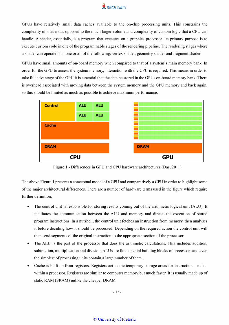
GPUs have relatively small data caches available to the on-chip processing units. This constrains the

complexity of shaders as opposed to the much larger volume and complexity of custom logic that a CPU can

handle. A shader, essentially, is a program that executes on a graphics processor. Its primary purpose is to

execute custom code in one of the programmable stages of the rendering pipeline. The rendering stages where

a shader can operate is in one or all of the following: vertex shader, geometry shader and fragment shader.

GPUs have small amounts of on-board memory when compared to that of a system’s main memory bank. In

order for the GPU to access the system memory, interaction with the CPU is required. This means in order to

take full advantage of the GPU it is essential that the data be stored in the GPUs on-board memory bank. There

is overhead associated with moving data between the system memory and the GPU memory and back again,

so this should be limited as much as possible to achieve maximum performance.

Figure 1 - Differences in GPU and CPU hardware architectures (Das, 2011)

The above Figure 1 presents a conceptual model of a GPU and comparatively a CPU in order to highlight some

of the major architectural differences. There are a number of hardware terms used in the figure which require

further definition:

• The control unit is responsible for storing results coming out of the arithmetic logical unit (ALU). It

facilitates the communication between the ALU and memory and directs the execution of stored

program instructions. In a nutshell, the control unit fetches an instruction from memory, then analyses

it before deciding how it should be processed. Depending on the required action the control unit will

then send segments of the original instruction to the appropriate section of the processor.

• The ALU is the part of the processor that does the arithmetic calculations. This includes addition,

subtraction, multiplication and division. ALUs are fundamental building blocks of processors and even

the simplest of processing units contain a large number of them.

• Cache is built up from registers. Registers act as the temporary storage areas for instructions or data

within a processor. Registers are similar to computer memory but much faster. It is usually made up of

static RAM (SRAM) unlike the cheaper DRAM

- 13 -

• DRAM or dynamic random access memory is the most common type of random access memory used

in computers today. Memory consists of an interconnected network of electrically charged points in

which a computer stores fast accessible data encoded in the form of binary values. DRAM is dynamic

in that unlike SRAM it needs to have its storage cells refreshed by giving it a new electrical charge

every few seconds. DRAM consists of a capacitor and a transistor. Capacitors tend to lose their charge

rather quickly hence the need for the constant refreshing. For a more in depth look at DRAM consult

Wang (2005).

As explained by Das (2011), GPUs contains many more ALUs than a CPU and far fewer components that

manage the cache and flow control of data. This means GPUs have a very high arithmetic intensity of operation,

meaning large amounts of computations versus memory operations. GPUs excel at high, parallel arithmetic

operations, which is exactly the type required by graphical applications in which clusters of pixels are allocated

simultaneous threads and rendered in parallel. GPUs are inefficient at handling many logical branches and if

used excessively in a shader, a noticeable degradation in performance will be the result.

In summary, a CPU is very good at executing a large number of different calculations on a small amount of

data whereas the GPU excels at executing a small number of calculation on a large set of data.

2.2 Software based rendering

Mileff & Dudra (2012) do a good job explaining in greater detail how software renderers work and this section

draws on work completed by them.

The rendering process is referred to as software based rendering when the entire rasterisation process is carried

out by the CPU instead of another dedicated graphics processor. Mileff & Dudra (2012) describe the rendering

process as follows: The geometric primitives are loaded into main memory in the form of arrays, structures

and other relavent data types. To produce an image on screen the CPU performs all the required processing

tasks such as colouring, texture mapping, colour channel contention, rotation, stretching, translation and any

other graphics processing requirements defined programatically by a developer. All of this processing is

performed directly on the data stored in the main memory bank situated on the main board. The results of the

processing are stored in a partitioned section of the main memory bank refered to as the framebuffer. The

framebuffer contains pixel data and transfers that data to the video controller. The video controller then

refreshes the screen ultimately displaying the image.

- 14 -

Figure 2 - General Graphics software pipeline (Mileff & Dudra, 2012)

Looking at Figure 2 recreated from the article by Mileff & Dudra (2012), we can see each function in the

pipeline that needs to execute in order to produce a final image. The process can be subdivided into two main

groups. The first section performs mainly vertex transformation operations which is everything outside of the

framebuffer area.

The second section is within the framebuffer and performs per pixel operations like triangle tesselation and

pixel shading. Optimisation in either group can lead to significant speed improvements. It is the framebuffer,

working on pixel based data, that is the most calculation intensive part and is often the source of the bottlenecks

in the graphic pipeline. It is possible to optimise the high calculation load via a CPU. This can be achieved by

using specific CPU based instruction sets like Intel’s streaming single instruction multiple data (SSE)

extension. This extension was developed for the Intel x86 architecture of CPUs.

CPU based optimisation techniques can add significant speed improvements to the rendering methods, but

they are still not currently as fast as GPU accelerated methods. That being said, CPU rendering does have

some advantages over the GPU based methods. A single component (the CPU) is used to control and compute

the whole pipeline. This means that there is less of a need to worry about compatibility issues as there is no

need to adapt to specific hardware achitectures. NVIDIA and AMD have their own proprietary hardware that

is used to make up the graphics hardware. As such some of the hard wired methods to peform the graphic

processing have evolved differently. This means that a software package developed for excution on the one

might not perform as well as on the other. Besides, for the compatibility considerations, a further advantage of

CPU based methods is that the entire pipeline methology can be programmed in one language. GPUs require

a shader language which is generally a low-level based language usually built up from a subset of C99 (a past

version of the C programming language standard). Furthermore the actual display of the image data is less

error prone as it goes through the operating system controller. This means that there is no need for a special

video card driver.

The main benefit of software based rendering is the greater flexibility available for the actual image synthesis.

There are drawbacks to using the CPU for rendering. The biggest issue is the use of main memory as the

storage medium. Any changes to an image or its constituent data requires the CPU to access the main memory

bank. The access time to this memory is usually high, requiring a large number of CPU clock cycles to complete

- 15 -

the action. Frequent changes to segmented data in memory causes significant performance issues. The second

problem is that in order to display the data on screen, the image has to be moved from main memory to the

video memory. The transfer speeds are limited by the communication bus. A 1027x768 image with a 32bit

color depth requires 3MB of storage. An image of this nature, for fluid graphics transition would need a

minimum refresh rate of 30 frames per second. This leads to an overall required transfer rate of 90MB of data

per second. The consistent refreshing of the screen is only required in immersive environments like the kind

found in 3D visualisations and gaming platforms. For a GIS application, rendering speed is important but the

method of display is different. Applications seldom require a continuous refresh of the entire scene as is the

case in games. Games use a loop to render at a framerate as fast as possible where applications tend to follow

an event driven approach. Only when something triggers an update does a section of the scene update.

2.3 Hardware based rendering

Hardware can either be designed to be flexible or highly efficient. There is a trade-off between the two. This

means designing for flexibility will most likely make it difficult to provide for optimised rendering pathways

which will impact on performance. GPUs are specialised, highly parallel microprocessors designed to offload

and accelerate 2D or 3D rendering to be used in conjunction with the CPU (Mcclanahan, 2010).

CPUs on the other hand have evolved to be general purpose processors. This means that the low-level circuitry

that makes up its core as well as the low-level code that maps to it have been designed for flexibility. This

flexibility comes at a cost of speed and efficiency. It is possible to build circuitry that is more optimised for

doing specific types of functions. The fact that there is a dedicated piece of hardware available for performing

the graphics processing means that the CPU changes its role from doing the processing to managing it and is

responsible then for facilitating data transfers from and to the GPU. GPUs are highly optimised for performing

graphic related calculations which have several appealing characteristics:

• The calculations are repetitive. A typical laptop screen with a resolution of 1200x800 has just under a

million pixels. Computer graphics require the running of the exact same program on each pixel (Blythe,

2008, p766). This maps really well to parallel architectures.

• Graphic data is highly segregated. Each graphic primitive needs to know little to nothing about its

neighbouring primitive.

The above-mentioned graphic attributes allow the GPU to implement two major optimisations:

• Force the logic concerned with what to do to be separate and external of the working logic and batch it

to all the workers. In other words telling 500 workers to do “x + z” for example.

• Use local data memory access (GPU memory) easing the connection of high volumes of GPU worker

threads, enabling them to access the required data to process. Threads access memory in a stepwise

multi block fashion.

- 16 -

The batching of processing and associated memory access model, which is optimised to work on smaller parts

of the larger whole, result in GPUs being bad at doing branch logic predictions. This is because all the

information is not available ahead of time for pre-processing, making it impossible to do effective predictions.

GPUs will and can handle branches but they do so very inefficiently. This inefficiency is caused due to the fact

that GPUs batch threads into what are known as warps and sends them down the pipeline as groups. This saves

on the instruction fetch/decode power. The term warp is applied to groups of threads executing in conjunction

on NVIDIA specific hardware. Other hardware often refers to the thread groups as single instruction multiple

data (SIMD) lanes. Data is processed in groups of warps and these warps usually consist of 16 to 32 threads.

The execution of calculations in these groups is the reason why branching should be avoided. If a thread

encounters a branch it may cause divergence. Branching logic pathways are split into different possibilities in

the same warp. In a 32 thread process, two threads may do the processing for a specific branch while the other

30 are left unused. In the next cycle the other branch may use 30 threads leaving 2 threads unused. Having

several nested branches will compound the problem causing a very inefficient pipeline where most of the

processing power is left unused. This needs to be kept in mind if using the newer OpenGL specification which

allows for the use of shader programs.

Also applicable is doing General-Purpose processing on Graphical Processing Units (GPGPU) via a library

like the Open Computing Language (OpenCL) platform which allows for the writing of programs that can

execute across heterogeneous computer hardware. This includes but is not limited to graphic hardware. This

concept is later explored when using GPGPU as a means of decompressing TopoJSON.

- 17 -

3 GEOGRAPHIC INFORMATION SYSTEMS

“The art, science and technology dealing with the acquisition, storage, processing, production, presentation

and dissemination of geoinformation is called geoinformatics” (Mankarie et al. 2010).

Geoinformatics provides a powerful sets of tools for collection, storing, retrieving, transforming and displaying

spatial data. The field consists of GIS, Remote Sensing (RS) and the Global Positioning System (GPS).

Mankarie et al. (2010) furthmore state that geoinformatics is an advancing science and technology, which can

be used for the research and development of other diciplines. For a geographer it can be a powerful tool for

the generation of data and attributes in support of the decision making process.

In this section we look at GIS in more detail while keeping in mind the end goal is to build a rendering engine

using OpenGL in order to assess its effectiveness. Firstly a GIS is discussed in terms of its constituent

components. Thereafter, various functions of a GIS are explored.

“A GIS is a computer system for processing, storing, checking, integrating, manipulating, analysing and

displaying data related to positions on the surface of the earth. It is then presented cartographically, graphically

or as a report” (Jebara, 2007).

With the vast amount of data available today, the potential for scientific study is large. Perkins (2010) is of the

opinion that as much as 95% of all newly acquired information can be linked in one way or another to a

geospatial location. All this data needs to be processed and stored in a format that allows for its fast retrieval

and rendering. Visualisation of very large amounts of spatial data becomes challenging. Quick high-quality

rendering is becoming more and more difficult to achieve as the amount of data increases. Such rendering is

essential for a fluid and dynamic computer application. When dealing with large datasets, complex memory

management and partitioning schemes are required.

A lot of the power inherent in GIS is derived from the human mind and its ability to interpret vast amounts of

visual data that can be captured within a single glance. This interpretation of visual data is termed visualisation

and applicable when the human mind is coupled with a generated “picture” of reality. Tory & Moller (2004)

define Visualisation as “a graphical representation of data or concepts which is either an internal construct of

the mind or an external artefact supporting decision making”. Alternatively conveyed, visualisations assist

humans with data analysis by representing data visually. GIS also has the power to relate a number of different

data types using the basis of common geography to reveal hidden patterns, relationships and trends that are not

readily apparent in spreadsheets or statistical packages, often creating new information from existing data

sources (Jebara, 2007). As an example, consider a large spreadsheet containing census data. The the number

of residents living at a specific address are listed. By using geocoding (the process of converting data such as

street addresses, or postal codes to corresponding lattitude and longitude values) it would be possible to build

a map showing population densities spread across an area. In a single glance it would be easy to find the area

- 18 -

of highest density. Due to the visual nature of the data being displayed, other conclusions may be drawn that

explain why there is a specific density associated with a particular area. Performing the same exercise by

reading over the raw data would take considerably longer.

It is interesting to note that current estimates state that 40% of the human brain is allocated for spatial

congnition and understanding (Lantzy, 2007, p. 6). This alone should highlight the importance of a GIS to

enable the visual analysis of otherwise massive amounts of highly abstracted data. It also shows why GIS

systems are so widely used in a diverse range of scientific fields.

A GIS is relient on the visual congnition of spatial data. This has led to the development of a number of

visualisation techniques. These techniques are useful considering the enourmous size that some datasets can

expand to. The upward trend in dataset size is driven by technological advancements in the field of remote

sensing which allows for higher resolution data capture. Higher resolution data allows for more accurate data

abstractions which in turn leads to improved geographic analysis. Larger datasets, of course, mean higher

rendering processing requirements. This once again shows that a faster, more efficient rendering engine would

be beneficial.

3.1 Components of a GIS

A GIS is complex and consists of more than just a computer system.

Figure 3 - Components of a GIS

A GIS comprises a number of components that form a complete system. As depicted by Figure 3 above, the

components include hardware, software, data, people and methods (Longley, Goodchild, & Rhind, 2003;

Buckey, 2014). Of importance in this study is hardware, software and data. Rendering a map requires

interaction from the computer hardware, specialised data structures to manage and manipulate the data, and a

software application to facilitate the functionality.

3.1.1 Hardware

The type of hardware that a GIS is running on determines, to a large extent, the operational speed of the system.

Additionally, it may influence the type of software that can be used due to specialised requirements. It also

determines the amount of detail that a GIS can house in terms of its data due to the higher computational

requirements of larger datasets. Visualisation speed is dependent on whether rendering is being performed on

a GPU or a CPU. Visualisation speed is also dependent on the processing power inherent in each of these

- 19 -

devices. Other important considerations are the access and data transfer speeds of the disk, system memory

and system communication bus which link all the hardware components together. Finally, the number of

hardware accelerators and CPUs contained in the system as well as the methods employed for processing, will

influence the total performance. GIS today runs on a diverse ecosystem of hardware configurations from

centralised servers to desktop computers used in standalone or networked configurations (Buckey, 2014).

Figure 4 - Intel Q67 Chipset (Intel, 2010)

In an attempt to determine the maximum theoretical throughput of data moving from the disk to the graphics

card, we refer to Figure 4. The main computer system used for conducting this study on, as well as all software

implementations, was a Dell Precision M4600 laptop containing an Intel Q67 Chipset. Most modern chipsets

have a similar layout; for this discussion the above block diagram will serve as a sufficient model to highlight

the path of data through the hardware.

It is important to understand the flow of data so that optimisations can be made at the correct places to ensure

the efficient rendering of data. Using the Intel Q67 Chipset, this discussion will focus on the hardware blocks

and how they influence the total data throughput of the computer system, all the way from storage to image

display.

To kick the discussion off and to trace the flow of data through the computer, let’s assume we have a

representation of an image encoded and stored on a data storage device. For the modern day computer there

- 20 -

are two practical options for persistent storage. The options are the mechanical hard disk drive (HDD) and the

solid state disk (SSD). Irrespective of the persistent storage medium used, the device has to be connected to

the SATA 3 connector on the main board (SATA 3 is the current standard at the time of writing). SATA 3 has a

max theoretical throughput of 6Gb/s which relates to 600MB/s, more or less (Serial ATA Revision 3.0

Specification, 2009).

As stated in the white paper by Dell (2011), HDDs are spinning mechanical disks. As such the mechanical

characteristics of the disk are instrumental in defining the resulting performance characteristics.

Figure 5 - Diagrammatic representation of a HDD (Cady, Zhuang, & Harchol-Balter, 2011)

Figure 5 shows the main constituents of a HDD in a very simplified manner. Cady, Zhuang, & Harchol-Balter

(2011) state that HDDs are the primary storage device in use for computers today. This is probably due to the

fact that they are relatively cheap to purchase. A HDD consists of a number of circular magnetic platters with

sectors arranged along tracks at different radii from the centre. A disk head hovers just above the platter and

performs read/write operations. Most HDDs have multiple platters with multiple heads. The heads are stacked

vertically and move in a synchronised fashion with respect to each other. To simplify the explanation a single

platter containing a single read/write head can be considered. Cady, Zhuang, & Harchol-Balter (2011) denote

that the main metric for disk performance is the average access time. The access time of a request is the time

between its arrival in the system and its completion. The disk access time can be subdivided into three parts:

• Wait time which is the time it takes for the head to move to the correct track.

• Rotational latency which is the time the head spends waiting for the platter to spin so that the correct

sector is under the read/write head.

• Transfer time is the time the actual read/write operation takes to complete.

- 21 -

A popular term used; is seek time which refers to the time needed to reposition the head between servicing two

individual requests. In other words, seek time consist of the wait time from the last request plus rotational

latency. Mechanically speaking the rotation speed of the disk, the size of the platters and the memory

scheduling algorithm controlling the head movement, play the biggest role in data transfer rates.

One possible method of increasing disk transfer rates is via the use of multiple disks in a redundant array of

independent disks (RAID). Cady, Zhuang, & Harchol-Balter (2011) state that this technique increases both

disk performance as well as fault tolerance. There are various RAID configurations available the most popular

being RAID0, RAID1 and RAID5.

Figure 6 - Most popular RAID configurations (Leurs, 2014)

These configurations are visually depicted in Figure 6 above.

RAID0 - Striping

Offers good performance in both read and writes with no parity control overheads. The full disk capacity of

all disks are utilised. There is no parity, so loss of a disk results in loss of all data. RAID0 is a good fit for non-

critical storage of data that has a high input/output (I/O) load requirement. This configuration works especially

well for rendering large amounts of data.

RAID1 - Mirroring

RAID1 offers very good read speeds. Write speeds are equivalent to that of a single disk. In the event of a disk

failure the array does not have to be rebuilt. The data just has to be copied to a new disk. The main downside

is that only 50% of the total disk capacity is available. The other disk is an exact duplicate essentially wasting

half of all possible storage space.

RAID5 - Parity across disks

Read operations are very fast in this configuration but write transactions are slower than a single disk. This is

due to the additional overhead of managing data parity. RAID5 is a good all-round system configuration that

- 22 -

combines efficient storage with excellent fault tolerance, yielding decent performance. It is commonly used

for file and application servers.

RAID arrays can also be used with SSDs. This usually results in excellent performance exceeding that of

HDDs. The associated cost is much higher though.

Some servers use a two tiered approach for configuring their storage area networks (SAN). The bottom tier

consists of a large number of HDD in a RAID configuration which uses the cheaper HDD storage space. The

top tier is a smaller array of SSDs which act as a data cache, reading and writing data to and from the bottom

layer of HDDs. This setup is cheaper than using only SSDs, but gives an overall better performance than

exclusively using HDDs. It is essentially the best of both worlds.

Dell (2011) allege that although the storage capacity of HDDs have increased 40% annually, their random I/O

performance has only increased at a rate of 2%. SSDs deliver superior performance but have higher cost

implications and smaller storage capacities. Another downside is an inferior lifespan compared to that of

HDDs.

SSDs are built from silicon memory chips. There are no moving mechanical parts and as such there is no

rotational delay and almost zero seek time which results in higher response times. SSDs provide big wins to

applications that need high performance as measured by access latency and I/O operations per second (IOPS).

Dell (2011) suggest that for applications that perform a lot of sequential workloads, HDDs are the better option

when considering price vs. performance. SSDs still offer superior sequential read/write rates though. For

random workloads SSDs are far superior to that of HDDs. In cases where applications require high IOPS, it is

worth investing in a SSD.

Databases are an example of a class of application that benefit from higher IOPS. Specifically, database indexes

which are responsible for speeding up searches and log files which contain the history of updates made to data,

will benefit largely. Log files are important to ensure atomicity, consistency, isolation and durability. These

attributes of a database ensure reliable transactions have been executed, keeping data in a consistent state.

Continuing the data flow discussion, the SATA connectors are attached to the chipset at the maximum

theoretical data rate of 600MB/s. Bourgie (2014) compares various HDDs and SSDs to determine the best

value for money based on price, performance, and reliability. He states that if considering only performance

the best HDD at the time of writing is the Western Digital Caviar Black and the best SSD is the Samsung 840

Pro. The Western Digital Caviar Black 4TB 64MB cache HDD has a max sustained read/write rate of 171MB/s,

(Western Digital, 2014). This is obviously nowhere near the upper limit of the SATA transfer bus. The Samsung

840 Pro SSD with 512GB storage on the other hand has a max read/write rate of up to 520MB/s, (Samsung,

2013). This is much closer to the max throughput of the SATA bus. Even so, the SSD is still the bottleneck and

there is room for a small amount of improvement of 80MB/s. In the best case scenario, using the more

- 23 -

expensive SSD option, data can be read from the storage system at 520MB/s. This means, if nothing is cached,

far better rendering performance will be achieved using a SSD then would be true of a HDD.

Continueing with the flow of data from the SATA bus, the chipset is connected to the main memory bank with

a 20Gb/s interface. The testing laptop contains two 8GB dual inline memory modules (DIMM) running in a

dual channel configuration. DDR3-1333 has peak transfer rates of 10667 MB/s. This, coupled with the ability

to run in dual channel, means effective data transfer rates of 21334 MB/s. To perform the actual memory

bandwidth calculations, you need the following information regarding the memory DIMM:

• Base DRAM clock frequency. This is usually measured in Megahertz (MHz). A hertz is the unit of

frequency defined as the number of cycles per second of a periodic phenomenon. It is the equavalent

to cycles per second where one Hz is equavalent to one cycle. one MHz is equavalent to 106 Hz.

• Number of lines per clock. The DDR3 memory range has two lines per clock.

• Memory bus (interface) width. DDR3 memory is 64 bits wide and is referred to as a line.

• Number of interfaces. Modern PCs typically use two memory interfaces to support dual-channel mode

so the effective bus width is 128 bits.

All the above mentioned information can be obtained by using an application like CPU-Z which exposes the

data.

Figure 7 - Dell Precision M4600 memory values

Figure 7 shows the information for the memory configuration on the Dell M4600.

- 24 -

In order to calculate the theoretical maximum bandwidth the following calculation can be performed:

Max Bandwidth = (665.1 x 106 ) clock cycles per second x 2 lines per clock x 64 bits per line x 2 interfaces =

170265600000 bits per second (19.8GB/s).

Looking back at Figure 4, the memory is connected to the CPU via a direct media interface (DMI) bus of

20GB/s which is just above the theoretical max transfer rate of the memory. So there is a small bottleneck at

this point caused by marginally slower memory.

The graphics card plugs into the PCI express port which is connected via a 16 lane 16GB/s data connection.

In short, the stored encoded image data will move from the disk via the SATA connection, through the chipset

into the CPU which will facilitate the storage of data into main memory. The data will have to be transferred

back to the CPU which will decode the data and put it into a data structure that can be used by the graphics

processor. Thereafter, it will be stored back in main memory. The data will then be streamed from main memory

to the graphics memory which usually has the highest bandwidth of all the components.

The card in the Dell M4600 is a NVIDIA Quadro 1000M which contains 2GB of GDDR 3 memory with a

bandwidth of 28.8GB/s. Therefore the main bottleneck in the complete system is moving data from the storage

device through the SATA connector to main memory. The max speed of the SATA bus is still sufficient for the

fastest HDD and SSD available at the time of writing. To get higher performance it will be necessary to keep

as much of the data as possible in main memory.

For optimal results, the data to be rendered should be kept on the graphics memory which will result in the

fastest possible rendering performance. Due to the size of some datasets, it may not be possible to store the

entire dataset directly in GPU memory. In such cases it is important to manage the caching and transfer of data

in an efficient manner. In a later chapter there is an experiment to try and use a form of data compression to

optimise the available space on the GPU. If the dataset is too large to fit in GPU memory, a partition scheme

of some sort will have to be devised to allow the image to be rendered as separate pieces.

3.1.2 Software

Software forms a broad ecosystem in a GIS application. It encompasses not only the main GIS package but all

the software used. This includes databases, drawings, statistics and imaging. The overall supported

functionality of the software stack will have an influence on the types of problems that a GIS can solve and

must match the needs and skills of the end user. Software can span multiple systems and does not necessarily

have to be housed and run on a single computer system. This can make it easier to purchase specialised

hardware systems that can be better utilised by the specific software. Also spreading software across multiple

nodes allows for higher computational throughput as each system only needs to provide a single service

allowing the full use of all the available computation resources towards that end.

- 25 -

Due to the fact that GIS application options can span multiple architectures and systems only strengthens the

arguments for OpenGL as a rendering engine. OpenGL is cross platform, meaning using a supported

programming language would allow for a rendering engine that could potentially run in any environment.

3.1.3 Data

Figure 8 - GIS layers overlaid to produce a final map image (United States Geological Survey, 2014)

As articulated by Guney et al. (2004), the world is infinitely complex and beyond our direct understanding and

modeling capabilities. The closer one looks, the more detail will become apparent to an almost infinite scale.

To store and process infinitely complex data is not possible. The solution to this problem is to create a data

abstraction that can be used to model a number of real world entities in a greatly simplified and generalised

manner. Not every detail about a feature provides useful information. As such it is only required to capture

data that will provide value for the specific study at hand.

Data can come from many different sources. Its quality and accuracy influences the final quality of the GIS.

Data impacts the type of questions that may be asked, as well as the scope of problems that can be solved. Data

in GIS is broken up into different layers as is depicted in Figure 8. Each layer can consist of a raster or vector

layer overlay. Each layer represents a specific theme (ESRI, 2012). The theme could, for example, be all the

lakes within a geographical region. Stacking layers on top of each other allows new information to be

discovered and helps to discern certain trends related to the specific goal of the study area. Think of the layers

in terms of transparencies used on a projector. Overlaying a number of them on top of each other creates a new

image composed of the underlying layers. Moreover each layer can be turned on and off giving the perception

of peeling layers on and off of the stack. The overlaying of data creates new images that highlight certain trends

that would otherwise go unnoticed. The GIS operator has final control over the map layer ordering and data

layers that comprise the final picture. Changing the ordering and playing with the layer featurisation promotes

data discovery. Featurisation is the grouping and styling of data layers by assigning certain visual cues like

- 26 -

colour, based on certain data attribute values. For example making all areas that contain a certain value blue.

This makes the specific data attribute stand out visibly on the map.

Geographic information is represented on a computer in either a raster data model or a vector data model.

Additionally this data can be augmented by tying in attribute data that represents additional data about the

spatial object that is not necessary spatial in nature, see Figure 9 below.

Figure 9 - GIS Data Models (Neteler & Mitasova, 2008)

The raster model represents features on the earth, for example land cover, as a two dimensional array of square

cells. The area represented by a square grid cell is computed from the length of its side and is called the raster’s

resolution. Resolution determines the amount of detail that has been captured. Raster images store data as a

2D matrix of pixels. 3D data can be stored as a 3D raster within a unit called a voxel, which is a volume pixel.

Raster models excel at representing continuous surface features like elevation, temperature and chemical

concentrations. These are sometimes referred to as a lattice (Neteler & Mitasova, 2008).

Although the raster model is mostly used to represent physical and biological subsystems of the geosphere

such as elevation, temperature, water flow or vegetation, it can also be used to represent lines and polygons

such as roads or soil properties. These attributes which traditionally are represented via the vector data model

can be representing using the raster model. Each cell has a single numerical value associated with it. This

numerical value may be used to represent colour, height or distance information. Raster images can be data

intensive. It is not uncommon for satellite images, which itself could span from a few meters to several

kilometres, to exceed several gigabytes. These datasets are not good at representing single feature objects as it

makes the application of certain algorithms, for example routing very difficult.

In the vector data model, features on the earth are represented as points, lines and polygons. Points are simple

feature types used as the building blocks for more complex features. The vector data model is defined by

Neteler & Mitasova (2008) as “being based on an arc-node representation”. Arcs are stored as a series of points

given by (x,y) or (x,y,z) coordinate pairs, or triplets (which contain height). The endpoints of an arc are refered

to as nodes. Arcs are coordinate pairs joined via lines. The points along a line are called vertices. Two

consecutive (x,y) or (x,y,z) pairs define an arc segment. The arcs form higher level features such as lines

(representing roads and streams) or areas (representing farms or forest lands). The arcs that outline areas

- 27 -

(polygons) are referred to as area edges or boundaries. Polygons are good at representing features like landuse,

lakes, dams, municipal boundaries and various other features with a minimal size overhead. Although polygons

can become quite complex they still serve as a generalisation of the objects they are meant to represent.

Attribute data is attached to features and represents the non-spatial aspect of data, for example, the name and

category of an object in the vector model and the cell value in the raster model. The process of relating attribute

information to a location is another useful feature offered by a GIS. The combination of the various attribute

values gives GIS different querying capabilities and allows for the study of interactions between various data

layer overviews.

It is possible to transform between the raster and vector data models. An example would be to take vector point

data which represent elevation in terms of coordinate pairs and then interpolate that into a raster map which

can be used to derive contour lines stored as numerical values in cells. Transformation between different data

models usually causes distortion and/or loss of spatial information.

Figure 10 - Data dimensions in a GIS (Neteler & Mitasova, 2008)

Figure 10 illustrates the dimensionality of data. The Earth and its features are located in 3D space and time. It

is sufficient in most applications to just use the 2D representations of geographical features. A geographical

feature is nothing more than the representation of a component of the earth. There are two different types of

geographic features. The first is a natural geographical feature which includes landforms and ecosystems. The

second type is of the artificial kind such as human settlements.

Elevation as a third dimension is sometimes stored as a separate raster map representing a surface within 3D

space. This is often incorrectly referred to as 2.5D.

- 28 -

Figure 11 - Differences in data dimensionality

We have throughout this text already made reference to 2D, 2.5D and 3D. To ensure the reader is comfortable

with the differences, refer to Figure 11 above. The figure depicts three different images. Image a represents a

2D map. In 2D there is no z values for each (x, y) coordinate pair. The end result is a flat image. Image b

presents a 2.5D map. In this perspective each (x, y) coordinate pair has a single z value. This gives the image

some depth but it is still not truly 3D. Image c depicts a full 3D model. It differs from 2.5D in that each (x, y)

coordinate pair can have one to an infinite number of z values.

3.1.4 People

People are the most important part of a GIS. They define and develop the procedures used in a GIS system.

Shortcomings in regards to the other four components can be mitigated by people, but the inverse is not true.

The multi-disciplinary nature of GIS means that a number of people with different skills are needed to work

together for the improvement and benefit of a GIS system. ESRI (2012) states that people are the ones that use

GIS to visualise, question, analyse, and understand data about the world. Without the visualisation processes

taking place, a GIS would not provide any useful information. Visualisation of speadsheet and database

attributes on a map adds several advantages, enabling people to perform spatial analysis of otherwise abstracted

data. This process allows for patterns and relationships to be discovered.

3.1.5 Methods

The methods in GIS are defined as the procedures used to input, analyse and query the data. The data is

important as it will influence the quality and validity of the final application. The methods are the steps that

need to be taken in a well-defined and consistent manner to produce correct and reproducible results.

- 29 -

3.2 Functions of a GIS

The basic functionality of a GIS follows a logical order in the form of data collection, storage, manipulation,

analysis, and presentation. Once all the required data has been collated and rendered to a map, the data can be

evaluated and then acted upon. The geographic approach helps with problem solving but the picture generated

that decisions are based off of are highly dependent on the quality of data. This section concentrates on the

process of data collection with the end goal leading to the generation of a map.

3.2.1 Data Collection

Figure 12 - The data collection process

Figure 12 show the basic data collection workflow used in GIS. Data collection can be performed by means of

a GPS, via classical measurement methodologies like surveying, aerial photography, and satellite imagery. The

manual digitising of maps can also be used to create digital content, but it is a time-consuming, manual process

that can be prone to error.

The collection process is also often referred to as data capture, data automation, data conversion, data transfer

and digitising. The process forms the basis by which informed decision making can take place. Good decision

making requires accurate and up-to-date information. Cay et al. (2004) attribute 60% of the total cost of a GIS

project to the collection of data.

The data capture workflow consists of:

• Planning which includes the establishment of user requirements, resources (people, finances, etc.) and

the development of a project plan.

• Preparation involves obtaining data, fixing poor quality sources, editing scanned images, setting up

appropriate GIS hardware and software systems to facility data loading. The key decision that needs

to be made in this phase is deciding whether data collection is to be done incrementally or once off and

to determine if the collection should be done in-house or via external resources.

• Digitising and transformation are the stages where the most time and effort will be expended.

• Editing and improvement covers techniques designed to validate data as well as fix errors and

improve quality.

• Evaluation is used to identify the quality of the work and determine if the project was a success or

failure.

- 30 -

There are two methods available for data capture: primary methods use direct measurement of the environment

such as a LIDAR survey; secondary methods use transfer methods which change existing datasets into a format

that can be utilised such as digitising.

Primary methods include raster and vector data capture. Raster data capturing is accomplished via remote

sensing techniques which are used to derive information about the physical world. The disadvantage of this

method is that data is often at resolutions that are too coarse. Vector data capture is done via surveying and

LIDAR systems.

Secondary data capture methods are available for both vector and raster data. Raster methods are usually

scanner based. Vector methods involve the digitising of objects from maps and other data sources.

The capture of attribute data which gets linked to the geospatial data can be entered by direct data logging or

manual keyboard entry. There are other methods of capture such as voice recognition and text recognition but

their accuracies are not high enough to make them practical.

3.2.2 Data Storage

The storage of data is fundamental in a GIS. File based storage methods have limitations with sharing

information across a multiuser base. For this and other reasons it is advantageous to use a database for storing

information. A Database Management System (DBMS) is a computer software program that is designed as a

means of managing all databases that are currently installed on a system. A database is a collection of

information that is organised so that it can be easily accessed, managed and updated. DBMSs have been highly

optimised for the storage of data, providing multiuser access to information, managing security and allowing

for the general management of data. Their centralised nature allows for specialised hardware to be purchased

on which to host the databases, which usually provides much better performance than would be possible on a

standard desktop computer.

Information is stored centrally, meaning there is always a single version of the data. Relational databases can

handle a variety of data types. Spatial databases contain all the benefits and use cases associated with a regular

database with the added benefit of being able to store, manage and manipulate location based data. Generally

the spatial information is stored in a specialised geometry type column which enables spatial queries to be

performed between objects in a layer and between different objects across different layers. The binary data

type used in the spatial data columns is often based on the Open Geospatial Consortium Inc. (OGC) well

known binary (WKB) representation for geometries. The internal storage of the geometry data is different

between the different DBMSs. At the very least, spatial databases support methods to convert from and to the

OGC’s WKB and well known text (WKT) representations.

Spatial databases allow for fast retrieval of data via data indexing schemes like the r-tree index. They provide

functionality for managing the spatial referencing systems of the data and allow for the projection of data into

- 31 -

different coordinate systems as required. They have useful spatial analytical functions that allow the execution

of queries based on spatial relationships. Spatial databases may also support raster images, network data

models, geocoding and routing. A non-exhaustive list of spatially enabled database systems are:

Oracle Spatial - An extension to Oracle allowing the storage and retrieval of multi-dimensional data.

PostgreSQL - This DBMS is a powerful open source object-relational database system. Spatial support is

provided through an extension called PostGIS.

MySQL - Another open source object-relational DBMS with spatial support.

SQLite - This little database is somewhat analogous to a Microsoft Access database. It consists of a few library

files developed in the C programming language. It provides spatial functionality very similar to PostgreSQL

via an extension called SpatiaLite. It is a popular database for mobile devices and yields exceptional

performance for smaller applications where multiuser access is of no concern.

Although file based methods are not always ideal for the storage and retrieval of spatial data, their use does

make sense in certain situations e.g. for a once-off spatial analysis. There are several popular formats available.

One of the most commonly used vector binary formats is the ESRI shapefile.

Shapefiles support the full vector data model comprising points, lines and polygons. Only a single feature type

is supported per feature class. A feature class is nothing more than a collection of geographic features of the

same geometry type. ESRI (2014) define a feature class as a dataset contained within a geodatabase. Feature

classes store geographic features which can be represented using points, lines, polygons, annotations,

dimensions and multipatches. A feature class stores simple features that can be organised inside or outside a

feature dataset. Simple feature classes stored outside of a feature dataset is a called standalone feature class.

Feature classes that store topological features must be contained within a feature dataset to ensure a common

coordinate system. The shapefile file format at its most basic level consists of three files. The main file (*.shp)

stores the geometries in a binary format. The index file (*.shx) contains an offset to the location of the geometry

contained in the main binary file. The dBase file (*.dbf) contains feature attributes with one row linking to one

feature.

The simplicity and ease of use of this format has made it one of the most popular formats for storing and

exchanging vector based geographical data.

3.2.3 Manipulation

A GIS contains a number of tools that allow the editing and conversion of data from one form to another. The

manipulation of data is not only applicable to spatial data. Attribute data can also be manipulated. An example

of this would be to combine area and population numbers to create a new value called population density.

Location data can be manipulated in many other ways. Some examples are coordinate thinning, geometric

- 32 -

transformations, map projection transformations, conflation, edge matching and interactive graphic editing. Of

interest for this study are transformations and projections.

Figure 13 - Geometric transformation (Schmandt, 2014)

Geometric transformation involves the warping of data stored in one layer to match that of data stored in

another layer. Transforms always involve the warping of data as visible in Figure 13.

Map projection transformations are concerned with the conversion of data from geographic coordinates to

other coordinate systems. If data is required to be in a different coordinate system, it will have to be

transformed. The representation of the round earth on a flat 2D monitor requires the conversion of geographic

coordinates to Cartesian coordinates. Various distortions occur as a result of the transformation process. The

affected properties are area, shape, direction, bearing, distance and scale. Projection of data will influence one

or more of these properties.

If a raster layer and vector layer are overlayed and the raster dataset is in a different projection system the

vector data is projected to match the raster data, as it is generally more complicated and resource intensive to

project raster based imagery. Projection systems form a pivotal part of a rendering system and it is one of the

more complex problems that has to be overcome when creating a rendering engine.

3.2.4 Analysis

GIS systems contain powerful mechanisms for use in data analysis. Xie et al. (2008) are of the opinion that it

is the analysis functions that fundamentally distinguish a GIS from other information systems. There are

numerous techniques available to aid in the analysis process. Some examples are measurements, layer

statistics, queries, buffering, filtering, map overlay, transformations and reclassifications. These techniques are

in support of network analysis, spatial interpolation, grid analysis, surface analysis and analytical modelling.

The vector overlay operations can be regarded as the most significant operations (Xie et al. 2008). Generally,

overlay functions require the vector data to be in a topological data model. If the original dataset is not in a

- 33 -

topological data structure, it will have to be processed and converted. This is a very time consuming operation

that is prone to error. Parallel architectures can greatly speed up this process. Speeding up topology creation

via GPU would be beneficial as it may result in some time savings. Further research would have to be carried

out in order to determine if it would be possible to offload processing to the GPU. Topology is defined later in

this dissertation.

3.2.5 Data Presentation

Figure 14 - Area by industry class

The visual presentation of data in a GIS, transforms raw data into 2D and 3D images which allow scientists to

reveal important trends and features inherent in the data. A GIS also has to be able to present non spatial data

that is linked to its spatial counterpart. This is usually done in the form of a grid or as labels on a map.

A valuable data presentation technique worth mentioning is that of map thematics depicted in Figure 14

(previously referred to as featurisation). Data is grouped together into similar or comparable values and then

styled according to the different groups. This immediately highlights spatial patterns and relationships between

groups and allows for easy interpretation of vast quantities of data within a single glance. Other display

possibilities are the use of graphs and statistics about the relevant geographic object which, depending on the

context, might make more sense.

- 34 -

4 COORDINATE REFERENCE SYSTEMS

A basic understanding of coordinate systems is important in this dissertation. Building a geographic rendering

engine will require working with geographic data in one or more map projections. Coordinate systems are

complex and all projection requirement are handled by the Proj4Net library. This library contains a full

implementation of geographic coordinate systems and coordinate transformation methods which makes

working with coordinate systems manageable.

Coordinate reference systems allow datasets to use a common set of values for integration. Although often

used interchangeably a distinction can be made between a coordinate system and a coordinate reference

system. A coordinate reference system is a system that is related to an object by a datum. A datum describes

the relationship of a coordinate system to a local reference which can be a point or a surface.

In GIS, the datum happens to be the geographic object, namely the earth. Without a datum a coordinate system

cannot uniquely identify a location via coordinate tuples and is merely an abstract mathematical concept that

can be applied to the practical problem of describing positions of features on or near an object. Coordinate

reference systems, coordinate systems and datums can each be classified into several types. In the realm of a

GIS it is a reference system used to represent the locations of geographic features, imagery, or GPS locations

within a common geographic framework. Coordinates belong to a coordinate system which consists of a

number of mathematical rules describing space (OGP, 2008).

Figure 15 - Surface of the earth (OGP, 2008)

- 35 -

The Earth is not a perfect sphere in shape (Figure 15). This requires surveyors to use simplified models to

represent the Earth as the real object is too complex to model perfectly. There are numerous models in existence

and each variation leads to a different coordinate system. This has the side effect that coordinates only represent

points on the earth unambiguously once the coordinate system has been fully specified (OGP, 2008).

The surface of the Earth is largely shaped by the gravitational forces applied to it. Surveyors use the

gravitational field to approximate mean sea level and the resulting model is called a geoid. It is an approximate

sphere but due to the rotation of the earth there is a slight bulging at the equator and a flattening at the poles.

Also due to variations in rock densities there are many local irregularities making the geoid a complex surface

model.

This study is focused on rendering geographic data which is most likely in one of the many different types of

coordinate systems available. In order to display this data in OpenGL, further coordinate transformation is

required. At the very least, a basic understanding of coordinate systems will benefit the reader. From the

perspective of designing a geographic rendering engine, a more in depth understanding of geographic

coordinate systems is required. The following section was compiled with extensive reference to ESRI (2004).

Each coordinate system is defined by:

• Its measurement framework which is either geographic (spherical coordinates that are measured from

the earth’s centre) or planimetric (coordinates that are projected onto a two-dimensional planar surface).

• Unit of measurement (feet or meters for projected coordinate systems or decimal degrees for latitude

and longitude.

• The definition of a map projection for a projected coordinate systems.

• There are other measurement properties such as a spheroid of reference, a datum and projection

parameters like one or more standard parallels, a central meridian, and possible shifts in the x and y

directions.

4.1 Coordinate reference system types

The OGP (2009) breaks down coordinate reference systems into six types:

Geographic 3D - A georeferenced 3D system that defines its axes in terms of latitude, longitude and ellipsoidal

height. GPS recievers typically operate using this type of coordinate reference system.

Geographic 2D - A georeferenced 2D coordinate system that is the same as the above 3D system, less the

ellipsoidal height values. It contains only the horizontal subset of the geographic 3D system.

Projected - A georeferenced 2D system with axes of eastings and northings where the axes may be referred to

as E and N or alternatively as X and Y. Projected coordinates are the result of applying a map projection to a

2D geographic system.

- 36 -

Vertical - A georeferenced 1D system with the axis representing height, elevation or depth. Height and depth

values are measured along the direction of the local gravity field.

Compound - A geographic 2D or projected coordinte reference system combined with a vertical coordinate

system. The horizontal and vertical components are independent, unlike a geographic 3D reference system.

Engineering - A non-georeferenced coordinate system in one, two, or three dimensions. 2D engineering

coordinate systems have horizontal axes identified by the values I and J. An engineering 1D coordinate system

has a vertical axis k. Engineering 2D coordinate systems include engineering site grids and 3D seismic binning

grids.

4.2 Geographic Coordinate Systems

Geographic coordinate systems consist of a spheroid, a sphere, the shape of the earth and a datum.

4.2.1 Spheroids and Spheres

In order to simplify the math used in projection systems the earth is often represented as a perfect sphere. This

is only sufficiently accurate for very small local areas. A more accurate approximation is modelling the earth

as an ellipsoid. For a visual reference see Figure 16 below.

Figure 16 - Difference between a sphere and spheroid (ESRI, 2004)

4.2.2 The Shape of the Earth

ESRI (2004) states that the shape and size of a geographic coordinate system defines the surface of the

projection. A geoid is a very accurate representation of the earth. Its complexity however necessitates the

simplification of its representation to the nearest mathematically definable figure. The earth is most accurately

represented as a spheroid (also called an ellipsoid) but to simplify the math it is often easier to assume that the

earth is a perfect sphere. Due to accuracy loss when representing the earth as a sphere, it is only viable for

maps that span small geographical areas (smaller than the scale 1:5000000). The scale of the map is the ratio

of distance on the map corresponding to the distance on the ground. For larger areas a spheroid should be used

if accuracy is of any concern.

- 37 -

Figure 17 - Major and minor axes of an ellipse (ESRI, 2004)

Figure 17 above denotes a spheroid or an ellipse. One way to create a spheroid is by rotating the semiminor

axis of the ellipse. This creates a rugby ball shape. ESRI (2004) notes that spheroids are alternatively named

oblate ellipsoids of revolution.

A spheroid can be defined by using the semimajor axis and the semiminor axis or alternatively by definition

of its flattening. “The flattening is the difference in length between the two axes expressed as a fraction or a

decimal” (ESRI, 2004). The flatting ranges from zero to one. A flattening of zero means the two axis are equal.

In other words the shape is a perfect sphere. The flattening of the earth is approximately 0.003353.

Over the centuries the earth has been surveyed a number of times. A spheroid that best fits one regions does

not necessarily fit another region. It is therefore important to determine the applicable ellipsoid before starting

a survey of an area to ensure accurate mapping. In summary, an ellipsoid determines the shape used in a

projection system and provides a best fit for the geoid (OGP, 2008).

4.2.3 Datums

A datum determines the position of a spheroid relative to the centre of the earth. It provides a frame of reference

for measuring locations on the surface of the earth. Changes to the datum will change the coordinate values of

the data as you are in essence changing the geographic coordinate system. The OGP (2008) notes that the size

and shape of the chosen ellipsoid is based on the best fit scenario for the geoid in the area of study.

Egbert & Dunbar (2007) highlight the importance of using the correct datum and state that the use of the

incorrect datum can result in an error of more than 300 meters. Depending on the precise details this error can

be larger.

- 38 -

Figure 18 - Error caused by using the wrong datum (Egbert & Dunbar, 2007)

Figure 18 above shows an example of a minefield that was surveyed. The area at the bottom was surveyed by

a team using an incorrect datum resulting in a shift of a few hundred meters. Depending on the scenario this

can have serious ramifications. Think of what would happen to a team tasked to remove the mines and being

completely unaware that they are in fact in the wrong area.

4.3 Projected coordinate systems

Projected coordinate systems are designed for flat surfaces such as printed maps or computer screens. Unlike

geographic coordinate systems, projected coordinate systems always have constant lengths, angles, and areas

across two dimensions (ESRI, 2004). Projected coordinate systems are derived from geographic coordinate

reference systems by applying a map projection. Locations are identified by x and y coordinates on a grid with

the origin at the centre. Each position has two values that reference it relative to that central location. The

coordinate values at the origin are at x=0 and y=0.

Figure 19 - The four quadrants showing positive and negative x and y values (ESRI, 2004)

Figure 19 above shows how the position affects the sign of the x and y coordinate pairs. The quadrant the

coordinate falls in will determine whether its values are negative or positive.

- 39 -

4.4 What is a map projection?

Figure 20 - The graticule of a geographic coordinate system is projected onto a cylindrical projection surface

(ESRI, 2004)

To represent a 3D Earth on a flat surface it is necessary to project it (Figure 20). The transformation of the 3D

coordinates to a 2D grid is called a map projection. ESRI (2004) explains performing a projection as follows:

visualise a light shining through the earth onto a surface called the projection surface. Imagine the Earth’s

surface is a clear transparent surface with a graticule drawn on it. Wrap a piece of paper around the Earth

forming a cylinder (as shown above) and turn a light on at the centre of the globe. Imagine that the shadows

cast by the graticule are burnt onto the paper. Unwrap the paper and lay it flat. The shape of the graticule on

the flat paper is very different from that which is shown on the round Earth. The map projection has distorted

the graticule.

It is not possible to flatten a round object without distorting the shape, area, distance or direction of the data.

Different projections cause different kinds of distortions. Most projections are designed to preserve one or two

of the data’s characteristics. Depending on the type of study being undertaken, the correct projection needs to

be chosen to ensure that the dimension that is of most importance is not the one being distorted. For example

if area calculations are of importance, an equal area projection should then be chosen, which may distort

distance for example but will maintain the area.

- 40 -

Figure 21 - Why distortion happens when coordinates are transformed (ESRI, 2004)

Figure 21 above shows why distortion occurs. Its cause is due to the projection plane being smaller than the

actual rounded surface of the Earth. It is not possible to place the larger amount of curved surface onto a smaller

flat plane. This directly causes the distortional effect.

Map projections are designed for specific purposes and a projection that might be suitable for large scale data

will not suffice for a small scale map. Projections designed for small scale data is usually based on spherical

rather than spheroidal geographic coordinate systems. Spherical coordinate systems use a simplified circle

representing the Earth where a spheroidal coordinate system uses a spheroid. Projections can be named by way

of the dimensions they preserve.

Conformal projections preserve local shape and this can only be done at local scale. It is not possible to

preserve the area of the Earth at global scale without causing distortions.

Equal area projections preserve the area of the displayed feature. In order to accomplish this the other

properties such as shape, angle and scale are distorted. In equal area projections the meridians and parallels

may not intersect at right angles.

Equidistant projections preserve the distances between certain points. Scale is not maintained correctly by

any projection throughout an entire map. There are in most cases one or more lines on a map along which scale

is maintained. Most equidistant projections have one or more lines for which the length of the line on a map is

the same as it is on the planet surface.

True direction projection or azimuthal projections maintain some of the great circle arcs giving the

directions or azimuth of all points on the map correctly with respect to the centre. Some true direction

projections are also conformal, equal area, or equidistant.

4.5 Projection Types

Maps are flat. In an attempt to simplify the projection process it is simpler to use projective surfaces that can

be flattened without stretching their surfaces. These surfaces are called developable surfaces and we have

- 41 -

already looked at one type of these surfaces, namely cylindrical. Other types include cones and planes. “The

purpose of a projection is to systematically displace locations from the surface of a spheroid to a representative

position on a flat surface using mathematical algorithms” (ESRI, 2004).

In order to project from one surface to another, the first step required is the creation of one or more points of

contact. Each point of contact is called a point or line of tangency. Planar projections are tangential to the globe

at a single point, where cones and cylinders touch the globe along a line (ESRI, 2004). Intersection of a

projection surface with the globe results in a secant contact surface. Irrespective of secant or tangential, the

points of contact are significant as there is no distortion on that point or line. These areas are true

representatives of the Earth’s surface and are often referred to as standard lines. In general, distortion increases

as the distance from the point(s) of contact increase. Projection types are classified by the projection surface

used: conic, cylindrical, or planar.

4.5.1 Conic Projections

Figure 22 - Conic Projections (ESRI, 2004)

The simplest conic projection is tangent to the globe along the lines of latitude. As visible by Figure 22,

meridians are projected onto the conic surface converging towards the apex of the cone. The parallel lines of

latitude are projected onto the cone as rings. The cone is then cut along any meridian to produce the final conic

projection (Figure 22, the right-most image). In this projection, lines of latitude form concentric circular arcs

and straight converging lines for lines of longitude (meridians). The plane at the large end of the cone,

perpendicular to the cut line, is called the central meridian. Remember that a standard parallel is a line of

contact. The further away you move from this line, either up or down, will result in an overall larger distortion.

Removing the top of the cone removes the area of the projection where lines are converging, leading to a more

accurate projection. Conic projections are used most often for mid-latitude zones that have an east-west

orientation.

It is possible to create more complex conic projections that have two points of contact. These projections are

called secant as previously mentioned and have two standard parallels. The distortion formed by this type of

projection differs between the two standard parallels as well as the areas above and below them. Generally

speaking, secant projections have less overall distortion when compared to tangential projections. An even

- 42 -

more complex conic projection is called an oblique projection. It does not line up with the polar axis of the

globe.

The representation of geographic features depend on the spacing of the parallels (ESRI, 2004). Equally spaced

parallels result in equidistant north-south areas that are neither conformal (preserve angles locally) nor equal

area.

4.5.2 Cylindrical Projections

Figure 23 - Cylindrical Projections defined by alignment of the central axis orientation to the globe

(ESRI, 2004)

Cylindrical projections can also be secant or tangent (Figure 23). The Mercator projection is one of the most

commonly used cylindrical projections with the equator used as the standard parallel. Meridians are

geometrically projected onto the cylindrical surface where the parallels are mathematically projected. This

produces a graticule where angles are 90°. The cylinder is cut along any meridian to produce the final

projection. Meridians are equally spaced where parallels have an increase in spacing towards the poles. This

is a conformal projection, preserving direction along straight lines. Cylindrical projections show no distortion

along lines of tangency and secancy, and are thus lines of equidistance. The other properties may vary

depending on the specific projection parameters.

4.5.3 Planar Projections

Figure 24 - Planar Projections (ESRI, 2004)

- 43 -

Planar projections project a section of the globe onto a flat surface. Planar projections are also called azimuthal

or zenithal projections. Planar projections are usually tangent to the globe at a single point but secant

projections also exist. Planar projections are region specific and the point of contact can be local to a specific

study area. Just like the other projection types there are three different aspects that define the projection namely:

polar, equatorial and oblique (Figure 24).

Polar is the simplest type. Here parallels are concentric circles centred at the poles. Meridians are straight lines

that intersect with their true angles of orientation at the poles. In the other aspects planar projections will have

graticule angles of 90° at the focus. The directions at the source are accurate. Great circles intersecting through

the focus are represented by straight lines. This means that the shortest distance from the focus to any other

point is a straight line. Area and shape are distorted in a circular shape around the focus. Azimuthal projections

accommodate circular regions better than rectangular regions. Planar projections are used mostly to map Polar

regions.

Planar projections can be further subdivided based on the view of data from a specific point in space (see

Figure 25).

Figure 25 - Planar Projections from different points of view (ESRI, 2004)

The point of view determines how the spherical data gets projected onto the flat surface. The perspective point

may be the centre of the Earth (gnomonic), a surface point directly opposite from the focus (stereographic -

viewed from pole to pole), or a point external to the globe as seen from a satellite (orthographic).

4.6 Projection parameters

Just defining the projection surface is not sufficient information for a complete coordinate system, (ESRI,

2004). Each map projection has a number of parameters that are required. The parameters specify the origin,

and customise a projection for the study area of interest. There are two types of parameter. Angular parameters

specify the geographic coordinate system units, while linear parameters specify the projected coordinate

system units. Look back at Figure 15 and note the values latitude (Φ) and longitude (λ). These two values

- 44 -

describe the positions of points relative to a geographical coordinate reference system (CRS) as described on

a coordinate system and represent an angular position (OGP, 2008). It is important to grasp that latitude and

longitude values are not unique unless the CRS has been defined. Without this definition an error of up to

1500m is possible.

A distinction can be made between linear and angular parameters. As the Proj4Net library is used for handling

projections it is not necessary to go into detail regarding the parameter themselves. Consult ESRI (2004) for a

more in depth explaination. For this study a proj4 string is passed to the projection library which sets up all the

required parameters. An example of this string looks like this: +proj=aea +lat_1=-24 +lat_2=-32 +lat_0=0

+lon_0=27 +x_0=0 +y_0=0 +datum=WGS84 +units=m +no_defs. This reasults in the Albers Equal Area

projection used in eastern South Africa using WGS84 as the defined datum.

4.7 Geographic Transformation

ESRI (2004) declare that at times it will be necessary to move data between different geographic coordinate

systems. The changes in coordinate systems are often associated with geographic transformations. Geographic

coordinate systems contain datums based on spheroids. Geographic transformations change the definition of

what that spheroid should be. There are a number of different methods available to perform the transformation.

Each method has its own set of trade-offs with a specific accuracy. Accuracy can range from centimeters to

meters depending on the method. The number and quality of the available control points used plays a major

role in the resulting accuracy.

ESRI (2004) articulate further that geographic transformations always convert geographic (longitude/latitude)

coordinates. Methods exist that can convert geographic coordinates to geocentric (x, y, z) coordinates and then

back again. The International Association of Oil & Gas Producers (2012) define a geocentric coordinate system

(GCS) “as a reference system based on a geodetic datum that deals with the Earth’s curvature by taking a 3D

spatial view”. This removes the need to model curvature. The origin of a GCS is at the centre of the Earth’s

mass. ESRI (2004) further declare that geographic transformation is always defined with a direction and the

transformation parameters describe how to convert from the input geographic coordinates to the output

geographic coordinate system. All transformation methods are invertible. This means that given a geographic

transformation, it can be applied in the opposite direction to end up with the same projection originally started

with.

- 45 -

5 OPENGL

In order to render any graphics, a graphics rendering API is required to act as an interface between the

programmer and the hardware. In developing a rendering engine for a GIS, the rendering API would form part

of the core functionality. This chapter helps give an overview of OpenGL which is used in designing the

rendering engine required for building the experimental rendering framework.

There are a number of ways in which OpenGL can be described. Segal & Akeley (2004) describe OpenGL as

the software interface to the graphic hardware consisting of hundereds of procedures and functions that allow

a programmer to specify the objects and operations involved in producing high quality graphical colour 3D

objects in the form of images.

OpenGL is an open, cross platform graphics standard with broad industry support. Its primary goal is to ease

the task of developing real-time 2D or 3D graphic applications. It does so by providing a mature, well

documented graphic processing pipeline that supports an abstraction of hardware accelerators (Apple, 2013).

Shreiner, Sellers, Kessenich, & Licea-Kane (2013) impart that the primary function of OpenGL is the rendering

of graphics into a framebuffer and it does so by breaking up complex objects into primitives (points, lines and

triangles), that when drawn at high enough densities gives the appearance of 2D and 3D objects. OpenGL is a

rasterization-based system. Other rendering system types exist that utilise alternative methods such as ray

tracing.

Rasterization techniques involve low-level sampling techniques which draw primitives by performing regular

sampling on the pixels that they cover. These systems draw their primitives in sequence, into a raster image

and handle occlusion by using an associated depth map. Later defined primitive may overwrite earlier

primitives if they are determined to be closer. Apple (2013) acknowledge OpenGL as an excellent choice for

doing graphic development due to it enabling an application to take advantage of massive concurrency, freeing

up processing power. Furthermore, OpenGL allows for the creation of higher resolution textures, detailed

models with complex lighting and shading alogorithms. Futher justification and benefits of using OpenGL

include:

• The OpenGL client-server model provides a reliable implementation that abstracts hardware details and

guarantees consistent presentation on any compliant hardware and software configuration. OpenGL has

a very well defined specification. All implementations have to adhere to this specification and go

through a vigorous conformance testing process before being marked as compliant.

• Applications can make use of the full computation power that the graphics hardware provides to

improve rendering speed and quality.

• The specification is controlled by a consortium called the Khronos Group whose members are made up

and form part of many major companies in the active computer industry space.

- 46 -

OpenGL at its core is a C-based API meaning it is extremely portable and widely supported. C integrates

seamlessly with Objective-C and many other development languages. OpenGL does not provide a windowing

layer of its own. It instead relies on functions defined by the operating system to integrate the drawing into the

windowing system. An application creates a rendering context and attaches to a rendering target. The context

manages the state changes and objects created by calls to the OpenGL API. A rendered object is the final result

of OpenGL drawing commands and is typically associated with a window or view.

OpenGL is implemented on the premise that the graphics hardware supports the use of framebuffers. A

framebuffer is a block of memory that is used to store image data. There can be multiple framebuffers. Double

buffering requires the use of two framebuffers. The back buffer is used to construct the next frame. Once

complete it is swapped to the front, displaying its content as a whole in a single instant. The previously front

buffer now becomes the back buffer and image construction starts anew. Utilising this technique allows for

smooth frame transitions and prevents certain graphic artifacts like partly completed objects or flickering

graphics from displaying on a screen. As long as there is enough memory available there can be any number

of framebuffers active. It is possible to prerender a frame ahead of time so that it will be avialable when

required. This can smooth the framerate for complex scenes but adds overhead and incurs larger memory use.

OpenGL cannot function without a framebuffer. In the event the computer system lacks a dedicated graphics

processor, OpenGL can make use of the CPU to perform all the rendering calls. If some or all drawing functions

are supported by dedicated hardware then hardware acceleration can be utilised to arguably add huge

performance gains far above what can be realised via the CPU. There are some arguments against whether this

is indeed the case. Lee et al. (2010) showed that it is possible to get really good performance compared to the

GPU, using highly tuned CPU code. In this case GPU implementations only have a 2X speedup over the

optimised software code. It is important to note that although it might be theoretically possible to optimise

algorithms on the CPU to achieve this performance, the time investment required may make this unfeasible.

From a programmer’s perspective, OpenGL is a set of commands used for the specification of geometric

objects in two or three dimensions including the commands that control how these objects are rendered into

the framebuffer (Segal & Akeley, 2004). It can be thought of as a very large state machine that can manage the

way objects are drawn to the framebuffer. OpenGL draws primitives using a number of selected modes where

each primitive consists of points, line segments, polygons or pixel rectangles (Segal & Akeley, 2003). Each

mode affecting the drawing may be changed independently, although the different modes interact as a

combined whole to determine what eventually ends up in the framebuffer. The setting of modes, primitive

specification and other OpenGL operations are described via commands sent in the form of functions or

procedures. The data defining an object which can be made up of positional coordinates, colours, normals, and

texture coordinates are associated with vertices. Each vertex is processed independently in order and in a

consistent manner. The same set of operations are performed for each pixel. This is the main reason why

- 47 -

graphics lends itself so well to single instruction multiple data (SIMD) processing. Segal & Akeley (2003) note

that there is an exception to this rule. The exception is relevant in instances where clipping is required to ensure

that the indicated primitives are contained within a predefined region. In this instance vertex data may be

modified and new vertices created. Another imporatant fact about OpenGL is that the order of vertex data

processing, executes in the same order orignially specified. This means that a single primitive must be drawn

completely before any futher objects can affect the framebuffer. Any query or pixel read operation must return

a state that is consistent with the complete execution of all previously invoked graphic library (GL) command

states.

The modern version of OpenGL has undergone major changes. There are a number of specifications that add

additional functionality for each version increment. For this dissertation we have focused on the OpenGL 2.1

specification and all code has been implemented using this version. OpenGL 2.1 was chosen as it has a large

suppport base. It generally ships as a standard part of all the big graphics card vendors support drivers. In the

rare occasion that a PC does not have it installed by default it can be downloaded and installed.

OpenGL 2.1 can execute drawing routines as part of a fixed function pipeline or it can swap out parts of the

rendering pipeline for custom shader based processing routines. For 2D rendering, only a small subset of

OpenGL is required. The fixed function pipeline is sufficient for the rendering tasks and there is no need for

the use of shader programs. The OpenGL discussion is specific to the OpenGL 2.1 specification defined in

(Segal & Akeley, OpenGL, 2006).

5.1 Hardware stack for OpenGL

Marsh et al. (2011) consider five pieces of hardware as important, when looking to process large amounts of

visual data. They are the graphics card, system memory, storage, networking and CPU.

The GPU is the primary factor for influencing overall graphics performance and has been discussed already.

Storage, CPU and HDD have also been covered in the preceding sections. Networking is of no concern for this

study as all experiments were performed in isolation on a single pc.

5.1.1 System Memory

System memory is the second biggest factor. The architecture of the CPU has an influence on the operating

system that can be installed. In a 32-bit operating system the maximum amount of addressable memory is 4

GB. On a 64-bit operating system the limit for theoretical purposes is unlimited1. To enable the execution of a

program or the manipulation of an image it must first be moved into the computer’s main memory. CPUs and

1 On a 32-bit CPU the max addressable linear memory is 2�� bytes or 4GB. A 64bit processor can address 2�� bytes

of memory. This is the theoretical upper limit as there would not be enough space for all the dual in-line memory modules

(DIMMS) (Intel Corporation, 2009).

- 48 -

GPUs have their own on-board dedicated memory. The GPU memory is often called Video Random Access

Memory (VRAM). VRAM cannot be upgraded so an upfront investment in a more pricey graphics card may

be cheaper in the long run.

5.2 Graphics terminology

The terminology discussed in this section draws heavily from the article by Apple (2013). There are a number

of terms that are used when working with OpenGL: render, renderer, buffer attributes, pixel format objects,

rendering contexts, drawable object and virtual screens.

The combination of hardware with the OpenGL specific software used to execute commands is termed a

renderer. The final image’s characteristics are dependent on the graphics hardware associated with the renderer

and the display device. Support for multiple renderers each containing their own set of capabilities or features

is made available via the OpenGL context. A large benefit of the programming model employed by OpenGL

is the extensibility afforded by the framework for hardware designers. It affords vendors the flexibility they

require to create better rendering hardware. Hardware vendors are free to implement their own extension

methods. This could mean that the same functionality may exist multiple times with different implementations

at the backend. If platform portability is important, it is better to stick with the OpenGL core platform and to

use an OpenGL Architecture Review Board (ARB) approved extension if available, rather than a vendor

specific implementation which might lock a developer into using a specific graphics hardware type. This might

not be a problem depending on the use case and could allow a programmer to make use of a highly optimised

feature that is only provided by that specific vendor. When new functionality becomes available it can be

incorporated into the core API if so decided by the ARB. OpenGL provides a query mechanism to get the

current OpenGL version as well as list all supported extensions and graphic hardware properties. This allows

for the runtime probing of functionality offered and allows the developer to define various implementations

based on the hardware capabilities of the specific graphics hardware.

Renderer and buffer attributes communicate their requirements to the OpenGL context which effects the final

renderer employed to perform a specific task. This is done by supplying specific attributes to an OpenGL

function call. The attributes describe things such as colour, depth buffer sizes and whether the image data is

stereoscopic or monoscopic. Renderer and buffer attributes are represented by constants which are defined

during design time.

Pixel format objects are opaque data structures that hold a pixel format along with a list of renderers and

display devices, describing the format for pixel data storage in memory. The definition itself contains the

number and order of components as well as their names which are typically red, blue, green and alpha.

OpenGL profiles are themselves renderer attributes used to request specific versions from the OpenGL

specification. Requesting a specific OpenGL version creates a renderer context that contains the complete

- 49 -

feature set specified for that version. Different versions can be used with the same code base only if the subset

of functionality is implemented in that profile.

Rendering contexts are usually just referred to as contexts. They are the primary object used when interacting

with OpenGL and contain all the state and object information. State variables are things such as drawing colour,

viewing and projection transformations, lighting characteristics and material properties. State variables are set

per context. Although multiple contexts are supported only a single context can be current on a thread at any

given time and the current context receives all OpenGL commands issued by the application.

Drawable objects refer to objects allocated by the windowing system that can serve as an OpenGL framebuffer.

It serves as the destination for the drawing operations and the behaviour is not OpenGL specific but defined

by the specific platform implementing the OpenGL specification. Drawable objects can be a full screen device,

off-screen memory (back buffer) or a pixel buffer. Pixel buffers are an OpenGL buffer designed for hardware

accelerated off screen drawing and as a source for texturing. Pixel buffers can be rendered into and changed

by OpenGL and then used as texture objects by the rest of the pipeline (Apple, 2013, p26). In order for OpenGL

to draw to an object, the object must be attached to a rendering context. The flow of data through OpenGL is

depicted in Figure 26.

Figure 26 - Data flow through OpenGL (Apple, 2013).

The combination of renderers and physical displays are called virtual screens. In a simple system containing a

single graphics card with a single physical display, there typically exist, two virtual screens. The one screen

consist of a hardware based renderer and the physical display. The other consists of a software-based renderer

and the physical display. OpenGL provides a software based fall back mechanism as previously mentioned. In

the event that the rendering hardware doesn’t support the requested feature it can be executed on the CPU via

a software based implementation. Care must be taken as this may cause performance degradation.

- 50 -

Figure 27 - A virtual screen (Apple, 2013)

Figure 27 portrays a virtual screen as the green rectangle around the image. It is important to note that a virtual

screen is not the physical display. The combination of the renderer provided by the graphics card and the

characteristics of the display create the virtual screen. The benefit of having virtual screens means that multiple

virtual screens can be displayed at the same time. This can be used for example in a CAD application to show

three different perspectives simultaneously. A virtual screen can be associated with multiple displays so that a

single image is displayed across all of them giving the illusion of one big screen.

An offline render is one that is not currently associated with a display and is not visible on any screens. The

application can enable them at any time by adding the appropriate rendering attribute. Taking advantage of

offline renders allows for a seamless experience when for example, a display is added or removed.

5.3 GL State

As discussed by Segal & Akeley (2003), OpenGL maintains many state variables. The variables can be

categorised by their function. Althought the operations themselves affect the framebuffer, the framebuffer is

not part of the state. The two main states are the GL server state and the GL client state.

- 51 -

Figure 28 - High level OpenGL breakdown (Apple, 2013)

Figure 28 clearly depicts the separation of layers in the GL architecture. OpenGL has been implemented as a

client-server model. A software application calling OpenGL functions speaks directly to the client. The client

then forwards the drawing commands to the GL server. The client, server and communication path between

the two are implementation specific. As an example the server and clients could be on different computers or

they could be on different processes on the same computer (Apple, 2013). The benefit of seperation allows for

graphical workload distribution between the client and server. The CPU can be loading data and munipulating

it into a specific format for processing by the GPU. Once the CPU has completed, data is passed to the GPU.

The CPU is now free to do any other processing task or get data ready for the next frame. So the architecture

allows for parallel asynchronous processing. Figure 29 below shows the hardware configuration which consists

of a client side that executes on the CPU and a server side which will execute on the GPU.

- 52 -

Figure 29 - Graphics platform model (Apple, 2013)

If OpenGL did not make provision for asynchronous execution between CPU and GPU, reduced performance

would result (Apple, 2013). There are certain commands that require synchronous execution and block until

complete. These functions need to be used carefully or they will adversely affect performance.

5.4 Context Creation

The OpenGL specification provides a rich set of cross-platform drawing commands but it does not explicitly

define the functions that interact with the specific operating systems graphics subsystem. A rendering context

is responsible for managing and keeping all the data stored in the OpenGL state machine. Multiple contexts

allow the state in one context to be changed by an application without affecting the other contexts (Apple,

2013; Segal & Akeley, 2003). If a computer contains multiple graphics processors, a different context can be

created for each one which can then execute independently. OpenGL is implemented by hardware vendors

using the following layers:

• An application layer which is responsible for using the graphics library by issuing drawing commands

to render a scene.

• A window system layer which is platform specific and responsible for managing the context creation

and state management of OpenGL.

• An OpenGL framework layer which contains the vendor specific implementation of the OpenGL

specification. NVIDIA, ATI and Intel for example will each have their own implementation in this

layer.

• The driver layer which is directly above the hardware contains the graphic layer driver plug-in interface

which allows the addition of third-party plug-in drivers. This enables third-party hardware vendors to

provide custom drivers optimised to best utilise their specific hardware.

5.5 Drawing to a window or view

The OpenGL specification provides hundreds of drawing commands that drive the underlying graphics

hardware. There is no windowing interface in OpenGL and without that the images are trapped inside the GPU.

- 53 -

The general approach for drawing a view or layer is as follows:

• Firstly, create an OpenGL context. Once available the renderer and buffer attributes that support the

OpenGL commands can be configured. The request from the operating system, a pixel format that

encapsulates pixel storage information and the renderer attributes are all context parameter

requirements. The returned pixel format object contains all possible combinations for renders and

displays available on the system that meets the requested requirements. This combination is referred to

as a virtual screen.

• Bind the pixel format object to the rendering context. The rendering context now keeps track of all the

state information that controls drawing attributes for each pixel. A pixel format object is required for

the creation of a context.

• After binding to a context, the pixel format object can be disposed of as its resources are no longer

required. Bind a drawable object to the rendering context. On the Windows platform that might be a

Windows form object. Make the rendering context the current context. All drawing commands are now

sent to this context.

• Execute the drawing commands to render your image on screen.

This section describes the high level methodology used for rendering data with OpenGL in general. Specific

libraries have their own set of specialised functions that need to be called. The overall idea remains the same

though. This next sections discusses rendering with OpenGL through the OpenTK API.

5.6 Drawing with OpenTK

OpenTK is an advanced, low-level C# library that wraps OpenGL. OpenTK is a free project that allows the

use of OpenGL, OpenGL/ES, OpenCL and OpenAL from the managed .NET languages (McClure et al. 2010).

The project started its life as an experimental fork of the Tao framework. Its original intention was to provide

a cleaner wrapper than that of the Tao framework. Where the Tao framework aims to wrap the OpenGL library

as closely as possible, OpenTK instead tries to leverage all of the syntactic benefits associated with the .NET

runtime. Examples are generics, strongly-typed enumerations and the separation of functions per extension

category. The OpenTK manual states that this library is suitable for games, scientific visualisations and all

kinds of software where the use of advanced graphics, audio or compute capabilities are required. Due to the

sheer amount of functions available, an OpenTK application can get very large and potentially complicated.

That being said, all OpenGL APIs follow a similar structure:

• Initialise the state associated with how objects should be rendered.

• Specify the objects to be rendered.

• Clean up the initialised objects.

- 54 -

To write an OpenGL application that exhibits maximum performance and low cost overhead the C/C++

language bindings approach will yield the best performance. Working in these languages is very tricky and

error prone. That being said, a programming language is only as good as a developer’s ability to express the

required functionality programmatically. A detailed comparison of programming languages is outside the scope

of this dissertation but here is a short list of some advantages offered by .NET and therefore indirectly by

OpenTK. Keep in mind not all the advantages are unique to .NET and C#:

• Garbage Collection - The .NET framework uses a garbage collector to manage the allocation and

release of memory for an application. There are two main types of memory an application needs to be

aware of. The stack and the heap. The stack stores simple types (value types) and pointers to reference

types. Any type that is defined as a class is a reference type. Each time a new object is created the

language runtime allocates memory for the object from the managed heap. As long as address space is

available in the heap the runtime will continue to allocate space to new objects. At some stage the

garbage collector must perform a collection in order to free up some memory. The garbage collector is

highly optimised to only perform collections during times when the effect on system performance will

be minimal. The collection process requires finding all the unused items, or items that have been

disposed of, and performs all the necessary clean-up operations. A programmer familiar with C/C++

will immediately understand the benefits from not having to manage all memory resources locally. A

large part of C/C++ applications consist of code to deal with memory allocation and deallocation. In

.NET this is taken care of for free by the library runtime.

• Array bounds checking - Ensures that a variable is within some bounds before it is used. It is used to

ensure a number fits within a given type (range checking) or that the variable being for example an

array index is within the bounds of the array. In .NET an exception is thrown by the runtime if access

to an index location outside the size of the array is referenced. Using pointer referencing to navigate an

array in C/C++ makes it is possible to exceed the bounds and even modify the memory outside of the

allocated array. This can result in a number of undefined problems and is very difficult to debug.

• A large collection of tools and libraries - The .NET library has an extensive application library which

makes developing applications easy and flexible. There are a number of libraries available to do just

about anything a software developer would require. This makes developing and prototyping

applications a pleasant and speedy experience.

• Exceptions have access to the execution stack - The execution stack keeps track of all methods that are

in execution at a given instance and is called the stack trace (Microsoft, 2014). The stack trace is

important as it provides a way to follow the call stack down to the specific line number in source code

where the exception occurred. This makes fixing errors in programming logic fast and easy.

• Advanced runtime type information and reflection - Reflection enables the runtime to obtain

information about loaded assemblies and the types defined within them such as classes, interfaces, and

- 55 -

value types. Reflection can be used to create type instances at run time and to invoke and access them

(Microsoft, 2014).

• Built-in support for threads - To provide a good user experience, applications need to do a lot of things

and some of these things can happen simultaneously. That coupled with the fact that most modern

computers have multiple processors available means threading is an essential function that a

development framework needs to expose in order to make use of the full computational potential.

Threading is a complex and difficult activity. The .NET Framework makes managing the creation and

synchronisation of threads easier, resulting in more stable software.

• No need for header files and #includes - .NET attempts to be more programmer friendly by being smart

enough to automatically resolve classes contained within the application domain. It does so by making

use of namespaces. A namespace is a name separated by the period character used to organise methods

and classes together. It also prevents clashes between functions and classes of the same name. There

can exist multiple functions and classes with the same name as long as they are specified in different

namespaces.

• Arithmetic operations can be checked for overflow if required - Overflow checking can be enabled via

compiler options, environmental configuration or the use of the checked keyword. Enabling the check

will cause the runtime to throw an exception that can be handled via program specific code.

• Objects must have a defined value before being used - In order to use a variable it needs to be explicitly

defined and have a valid value. If this is not the case a null reference exception will occur. This provides

another mechanism to check that the application logic is correct.

There are some downsides to the .NET Framework. It is only fully supported on the Windows operating system.

There are ways to use C# on Apple and Linux systems but the feature support is only a subset of the complete

framework. C/C++ can arguably provide better performance than .NET. The speed debate can be argued to ad

infinitum, but this is the generalised view. The main point is that .NET is fast enough and most importantly a

user friendly object oriented language.

- 56 -

Figure 30 - OpenGL primitives (OpenTK, 2014)

All the OpenGL commands used in this dissertation were executed through the OpenTK library.

When it comes to drawing in OpenGL, there are basically two options for specifying the rendering of objects

(OpenTK supports both). The first is called immediate mode drawing and works by manually specifying each

vertex to be drawn by using a set of drawing commands which are contained within a GL.Begin(<Primitive

Type>) and a GL.End() statement (OpenTK, 2014). Immediate mode drawing does not maintain any of the

defined vertices that serve as the building blocks for other primitive types. As such, every frame needs to

upload the full data model in order to render it again. Figure 30 shows the list of primitives available in OpenGL

which will be dicussed shortly. Each frame drawn using GL.Begin() and GL.End() require the objects to be

fully specified for each frame. This is true even if nothing in the image has changed. The CPU has to constantly

transfer the data across the communication bus causing massive overhead.

Immediate mode drawing is the only drawing mode supported by GDI/GDI+ and it is later shown that even

using this suboptimal drawing method in OpenGL, results in a higher rendering performance exceeding the

previously mentioned software rendered APIs.

The other drawing method requires specifying arrays of vertices to be drawn. The arrays, which can be

interleaved with other drawing attributes are then passed off to the graphics processor using Vertex Buffer

Objects (VBOs) or display lists via a single command. The data is then stored in GPU memory for later reuse.

This method of drawing is optimal. The features need only be fully specified for the first frame. Thereafter it

is only necessary to update changed vertices. There is much less communication required across the PCI

express bus as the bulk of the data is maintained in GPU memory which is usally much faster than main

memory, resulting in additional performance gains.

- 57 -

GDI does not support the use of VBOs or display lists. It is possible to specify the primitives by passing an

array of drawing attributes so that only a single call is made. This does increase drawing performance but not

to the extent of what OpenGL provides.

OpenGL supports a number of primitives which serve as the building blocks for more complex object

geometries. All objects can be specified using three main groups: points, lines or triangles.

Shreiner, Sellers, Kessenich, & Licea-Kane (2013, p84), explain the primitive types in detail: points are

represented via a single vertex which consists of a point in four dimensional homgeneous coordinates. Points

don’t contain an area but they are mapped to the smallest part on a monitor. They end up as a single square

area represented by a pixel on a monitor or a memory address in a framebuffer. In rendering a point OpenGL

determines which pixels are covered by the point using a set of rules called rasterization rules. The rules for

rasterizing a point in OpenGL considers a sample covered by a point; if it falls within a square centered on the

point’s location in window coordinates. The side length of the square is equal to the point’s size, which is a

fixed state controller by the glPointSize() command or the value determined by a geometry shader program.

By default, OpenGL renders a point as size 1.0 which translates to a single pixel on the screen. This is assuming

it is not clipped and falls within the viewing area. A value larger than one would lead to multiple pixels lighting

up. If a point’s vertex lies exactly midway between two horizontally or vertically adjacent pixel centers, then

both of those pixels will be lit. If the point’s vertex lies at the exact midpoint between four adjacenet pixels,

then all four pixels will be lit for a total of four pixels per point (Shreiner, Sellers, Kessenich, & Licea-Kane,

2013, p87).

In order to render points in the correct location, a coordinate system is required. There are a number of different

coordinate systems in use by OpenGL. Homogeneous coordinates are one such type. Kesteloot (2006) explains

homogeneous coordinates as a coordinate consisting of four dimensions (x, y, z, 1). Homogenous coordinates

are important as they enable translations, rotations and scaling to be done via matrix multiplication. A 2D

matrix is incapable of performing a translation, which is nothing more than the moving of all points along the

same direction and distance. It is not possible to write a 2D matrix that can move all points up by two units

and right by three units for example. The matrix is multiplied by each point and multplication can’t act like an

addition. If the graphics pipeline was made up entirely of 2D matrices it would require the numerous

translations to be accomplished via another method.

Kesteloot (2006) shows that if your desired result is to take a set of points, rotate it, translate it, then rotate it

again you’d be forced to write it as P' = R2 × (T + (R1 × P)). Each point (P) goes through a multiplication

(R1), then addition, and finally another multiplication (R2). If not for the translation the simple multiplication

of the two rotation matrices together (matrix multiplication is associative meaning that for any three numbers

a,b, and c: (a * b) * c = a * (b * c) would suffice. In short the multplication of the first two values followed by

the multiplication of the third value would still yield the same result. Each point would just be multiplied by a

- 58 -

single matrix saving a lot of processing time for each vertex on a potentially large data model. This is where

homogeneous coordinates come in as they allow the expression of a translation as a multiplication so that all

matrices can be collapsed up front. This results in an optimised mathematical transform.

Triangles are made up from a collection of three vertices. When separate triangles are rendered, each triangle

is independent of all the others. A triangle is rendered by projecting each of the three vertices into screen space

and forming three edges running between the points. When defining multiple triangles it is inefficient to define

duplicate vertices. In such cases it may be better to use triangle strips or triangle fans. In a triangle strip the

first triangle requires the specification of three vertices. Thereafter each vertex creates a new triangle. A triangle

fan works similarly but the different triangles share the same first vertex creating a fan like object. Refer to

Figure 30.

Polygons have two different sides, the front and the back and it might be rendered differently depending on

which side is facing the viewer (Shreiner, Sellers, Kessenich, & Licea-Kane, 2013, p90). This enables cutaway

views of solid objects in which there is an obvious distinction between the parts that are inside and those that

are outside. By default both the front and back faces are drawn the same. To draw only outlines or vertices

requires the use of the glPolygonMode() function. OpenGL convention dictates that polygons where vertices

appear in counterclockwise order on the screen are called front facing polygons. The orientation is also called

its winding. In a completely enclosed suface constructed from opaque polygons with a consistent orientation

none of the back facing polygons are ever visible. Enabling culling will discard these polygons and give a

performance increase. This can be enabled by using the glCullFace() function.

To render a simple triangle using OpenTK, there are two main controls that could potentially act as the canvas

for rendering the scene on. The first is a GameWindow class. This class provides numerous methods that can

be overidden. Some functions of note are the OnLoad() function which executes once, directly after the

OpenGL context has been initialised. The other functions are the OnRenderFrame() method which provides a

place holder for adding the frame rendering code and the OnResize() functions which modifies the viewport in

the event that the window is resized. The GameWindow class works by providing a game loop which is a

control loop that executes infinitely as fast as the computer’s hardware will allow. It is really designed for use

in games where the highest framerate possible is beneficial. Although it is possible to build a GIS viewer using

this class it is probably not the optimal control for it. Game design requires a sligtly different workflow and a

way to keep track of the static state of the game world. The game loop acts as the entry point for three main

stages to take place:

1. Stage 1 gets the state of all inputs to and from the system.

2. Stage 2 takes all the current information at hand and does a number of calculations to update the game

world.

- 59 -

3. Stage 3 is responsible for updating all the pixels on the screen to reflect the current state of the game

engine.

The other more relevant control provided is the GLControl. Instead of an event loop this control uses window

events which only updates the scene when explicitly triggered to do so. This can happen programatically or

via some window drawing call that forces a window paint event to fire. The GLControl provides a lot more

control and access to low-level OpenGL functions. This low-level access is more abstracted in the

GameWindow class. OpenTK (2008) states that this route should be followed if any of the following conditions

hold true:

• You require a rich user graphical interface application such as CAD, GIS and game level editors.

• You want to have an embedded OpenGL rendering panel inside an already existing Windows Forms

application.

• You want to be able to do drag and drop operations into the rendering panel.

To build a basic OpenGL application using the OpenTK library requires the initialisation of a new .NET

Windows application and include the required library files. Once complete, simply drag a GLControl to a form

in the Visual Studio designer. It is important to note that no change or access to any of the OpenGL state

functions or variables are allowed until the OpenGL context has been initialised. When working with .NET

forms the events happen in the following order:

1. The main forms constructor runs.

2. The Load event of the form is triggered.

3. The Load event of the GLControl is triggered.

Only after the 3rd step above has completed will the OpenGL context be intialised and be available to the

application. Attempting to access the context before this time will result in exceptions.

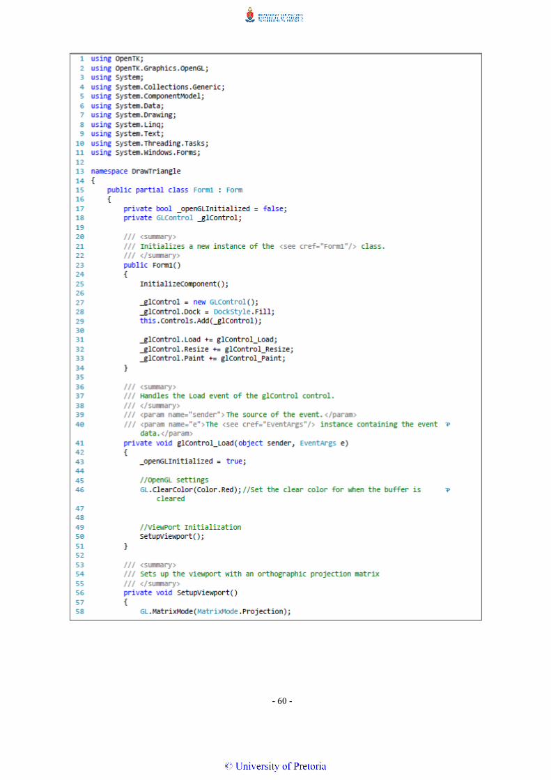
- 60 -

- 61 -

- 62 -

Figure 31 - OpenGL with OpenTK a first example

Figure 32 - Execution timing result of Figure 31

Figure 31 shows the very basics of drawing a single triangle using OpenTK with the resulting image shown in

Figure 32.

Line 1 through 11 are using the directives which add the required types into the current namespace so that it is

not necessary to fully qualify the types used in the program. For example if using OpenTK.Graphics.OpenGL;

was not in the file the fully qualified function name would have to be written out, for example,

OpenTK.Graphics.OpenGL.GL.ClearColor(Color.Red) instead of the current GL.ClearColor(Color.Red).

Line 23 is the forms default constructor and is the first function to execute in the class. Line 25 sets up the

form and any controls that were added via Visual Studio’s design time designer. Line 27 to 29 is creating the

OpenTK GLControl object that will be used to display the OpenGL rendering and adds it to the current form.

Line 31 to 33 sets up the GLControl’s events and maps them to their corresponding functions. After the form

constructor has completed, Line 74 (the form load event) is executed which in this example does nothing.

Thereafter the GLControl’s event handler is triggered (Line 41). There are some other window form events

that fire before the GLControl’s load event, for example the form resize event (Line 84). As you cannot call

OpenGL functions before the GL context has been initialised, a check has to be built in that can maintain if the

OpenGL context has been initialised. The boolean variable defined as _openGLInitialised starts with the initial

- 63 -

value of false and after the GLControl load event fires, explicitly sets its state to true. This variable can then

be used as a guard to ensure that the context has been initialised before executing a GL call (Line 87

demonstrates this). The GLControl load event is a good place to set GL state variables. In this case Line 46 is

setting the clear colour that OpenGL should change the background to when the buffer is reset. This example

specifies that the entire buffer is to be set to red. Another very important method that should be set during the

OpenGL control load event is the viewport. The viewport specifies the affine transformation of x and y from

normalised device coordinates to window coordinates. Normalised coordinates are coordinates that fall with

the range of -1 and 1. This allows for scaling and mapping from the drawing buffer to the display window. The

SetupViewPort() function on line 56 is responsible for setting up the world coordinate system and does so by

firstly telling OpenGL that we wish to modify the projection matrix.

A computer monitor is a 2D surface and as such to render a 3D scene, the scene must first be projected onto

the screen as a 2D image which is accomplished via the projection matrix (Ogoerg, 2012). As futher explained

by Ogoerg (2012) the projection matrix is a mathematical matrix that specifies the transformation that

transforms all vertex data from the eye coordinates to clip coordinates. The clip coordinates are also

transformed to the normalised device coordinates by dividing with the w component of the clip coordinates. It

is useful to keep in mind that both the conversion to normalised device coordinates and clipping take place via

the projection matrix. Clipping is performed in clip coordinates before the conversion to normalised

coordinates happens by dividing by the w component.

At this point the OpenGL API is aware that it is the projection matrix that is to be modified. The next function

on line 59 sets the projection matrix to an identity matrix (Figure 33). The identity matrix is a special matrix.

When multiplying a vector with an identity matrix the result is a vector that is unchanged. Matrix multiplication

is cummulative, so the identity matrix is a way to reset it to a default state.

Figure 33 - Identity Matrix

Line 62 sets up an orthographic projection. There are two options when it comes to the world coordinate

system. You can use an orthographic projection as shown in this example or a perspective projection which

more accurately models how humans perceive the world.

- 64 -

Figure 34 Perspective and orthographic projection

The left image in Figure 34 denotes a perspective projection and the right hand figure shows an orthographic

projection. Humans are used to perspective viewing which makes further away objects seem smaller.

Orthographic projection usually looks strange as objects have a constant size irrelevant of the viewing distance.

Orthographic projections are useful in applications like CAD and object modelling as it is easier to draw and

judge proportions. Perspective projections are most often employed in gaming engines where a more realistic

scene is required.

Line 62 sets up the orthographic projection with the point (0,0) starting in the left bottom corner and extending

up on the y axis and right on the x axis to an amount equal to the size of the viewport. Line 66 maps the

viewport. The result of the two lines of code is a viewport with a 1:1 mapping to the world coordinate system.

It is important to note that screen coordinates usually start at the top left where OpenGL by default starts at the

bottom left. After the GLControl’s load event has fired, the viewing projection is defined and setup. Line 104

now executes which is the paint event of the GLControl. As with the resize event there is a check to ensure

that the OpenGL context has been initialised. Line 110 clears the colour buffer as well as the depth buffer. This

resets the background to the colour defined by GL.ClearColor() on line 46. Next on line 114 the modelview

matrix is changed. This matrix defines the coordinate system relative to the object being rendered. The default

matrix value is set to the identity matrix so that any other changes to the matrix are reset to the origin of the

world coordinate system. The drawing colour which will be used to render the triangle in is set to green on line

116. OpenGL is a state machine and as such any objects rendered after this command will be green until it is

changed again. Next is the part that actually sends the draw commands to OpenGL. Immediate mode drawing

is being used which requires all drawing to happen in between a GL.Begin() and a GL.End() function. The

GL.Begin() function takes a single argument in which it sets the primitive types that is to be drawn. Line 118

sets the drawing mode to triangles. This means for every three vertices specified a triangle will result. To render

two triangles, requires the specification of six coordinates. GL.End() tells OpenGL that the rendering group is

complete.

- 65 -

By default, OpenGL uses double buffered rendering. So all the drawing calls executed thus far have only

affected the back buffer which is not currently visible. In order to show the changes, OpenGL is required to

swap the buffers. Line 127 moves the back buffer to the front which is then shown on screen. The previously

front buffer now becomes the back buffer on which the next frame can be prepared. Any changes required to

be made to the image can be made on the now current back buffer and then quickly swapped back again.

By swapping between the front and back buffer at a rate of at least 30 frames per second we get a fluid movie

like effect. This is not required for a GIS viewer. We only require a refresh if the view changes.

This example illustrates a simple exercise using OpenGL, with the end result visible in Figure 32.

There are a number of problems with the way the rendering has been done. Firstly, immediate mode drawing

has be utilised, which is not the most effective way to do rendering in OpenGL. The problem with immediate

mode drawing is that the graphic card is directly linked with the program flow. The driver cannot tell the GPU

to start rendering before the GL.End() function. So while adding vertices between GL.Begin() and GL.End()

the graphic card is waiting. The vertices are added to local memory and only after GL.End() can OpenGL

transfer the data to the GPU and perform the rendering. The GL.DrawArrays() function is also an immediate

mode drawing function except it supports passing an array of vertices to be drawn.

The second problem is attributed to OpenTK. The manual states that there is a 20ns execution call cost due to

the marshalling that needs to happen between the .NET managed code and the compiled OpenGL driver code.

The recommendation is to not exceed more than about 500 OpenGL calls per frame. Using immediate mode

drawing with a large model will easily exceed this recommended limit. The better option would be to use

VBOs which we will discuss later.

The third problem is not really a problem per se, but can be attributed to the method by which drawing takes

place in OpenGL. Games require fast consecutive frames to give the perception of motion. When designing a

GIS application a better option would be to render the current view and save it to an image which can then be

displayed. If the view changes due to for example panning the map, it would only be required to redraw the

section on the side that has changed, essentially preserving some of the previously processed image data. This

will result in better utilisation of computing resources. There is some overhead of copying the data from the

framebuffer to a bitmap object but drawing on data from performed experiments, the overall result is still faster

than what can be expected from purely using the GDI/GDI+ APIs. This method of preserving the already

processed data does seem to be the preferred way of rendering GIS views if considering existing packages like

SharpMap, MapWindow and QGIS.

- 66 -

5.7 Viewing in OpenGL

After stepping through the basic example shown above the following section on viewing may be clearer. In

this section we aim to provide a lower level explanation of how a scene is constructed mathematically in

OpenGL and how we can manage the different coordinate systems. This section draws on the work by Shreiner,

Sellers, Kessenich, & Licea-Kane (2013, p205-258).

In a typical OpenGL scene there are multiple objects, each with their own independent coordinate system.

These object need to be transformed (translation, scale and oriented) into the current scene. After translating

and setting up the different objects within the scene, the scene itself needs to be viewed from a particular

location, direction, scaling and orientation. The mapping of a typical geometric object directly to device

coordinates would not depict much. This is due to the fact that the model’s coordinate system range will in all

likelyhood exceed that of the device’s. For this reason OpenGL uses a model of homogenous coordinates

where the model gets mapped to the range (-1, -1) and (1, 1). The key to mapping a 3D object to a 2D display

is the use of a viewing model which uses homogeneous coordinates, the use of linear transformations via

matrix manipulation and viewport mapping.

For the time being it is easier to keep thinking of objects as being 3D. We will later discuss the transformation

to a flat 2D image.

Figure 35 - Steps in configuring and positioning the viewing frustum (Shreiner, Sellers, Kessenich, &

Licea-Kane, 2013, p207)

- 67 -

Shreiner, Sellers, Kessenich, & Licea-Kane (2013, p205-258) explain the steps in viewing by way of Figure

35.

• Step 1, move the camera to the location to shoot from and point the camera in the desired direction

(viewing transformation).

• Step 2, move the subject to be photographed into the desired location in the scene (modeling

transformation).

• Step 3, choose a camera lens and adjust the zoom (projection transformation).

• Step 4, take a picture (apply the transformation).

• Step 5, stretch or shrink the resulting image to the desired picture size (viewing transformation). In a

3D scene this stretching and shrinking is applicable to the depth as well.

Step 5 is not to be confused with step 3 which determines how much of the scene to capture, not how much to

stretch the result. Also note that step 1 and step 2 can be thought of doing the same thing but in opposite

directions. Moving the camera away from the subject has the same result as moving the subject away from the

camera. Moving the camera to the left is the same as moving the subject to the right. Rotating the camera

clockwise is the same as rotating the subject anticlockwise. It is up to the developer to decide what movements

to perform as part of step 1 with the remainder belonging to step 2. It is due to this reason that step 1 and step

2 are usually combined into a single model-view transform. It still consists of a number of translations,

rotations and scalings. The defining characteristic of this combination is to create a unified space for all the

objects assembled into the scene called eye space. OpenGL requires that the defininition of the transformations

for step 1 to step 3 are specified.

To make processing more efficient any object that falls ouside of the viewing frustum is clipped. The left-most

image in Figure 34 shows a perspective projection. It looks like a pyramid with the top cut off. The smaller,

top side is called the near plane and the larger base is called the far plane. Any item that is specified outside of

these two planes and the volume created by them is culled from the image. This makes processing more

efficient as vertices that are not going to be used are discarded early in the rendering process. In cases where

objects exist partly outside of the viewing frustum the objects are cut along the plane of intersection. In

OpenTK the orthographic view is defined using this command:

GL.Ortho(double left, double right, double bottom, double top, double zNear, double zFar);

A perspective projection is defined like this:

GL.Frustum(double left, double right, double bottom, double top, double zNear, double zFar);

All viewing in OpenGL is accomplished via a series of matrix manipulation.

- 68 -

Figure 36 - ModelView Matrix (Ahn, 2013)

Ahn (2013) has an informative article explaining the different transformations that take place during OpenGL

viewing. The above figure (Figure 36) give a good overview of how the modelview matrix works. The

rightmost column (m12, m13, m14) are used in the translation of the objects. m15 is the homogeneous

coordinate specificially used for projective transformation. The other three element sets (m0, m1, m2) (m4, m5,

m6) and (m8, m9, m10) are used for Euclidian and affine transformations such as rotations and scaling.

Viewing in OpenGL can become really complex. The OpenTK API does attempt to simplify the process by

providing functions and abstractions. It is required to understand what is happening in the background if a

view is to be rendered with an expected outcome.

This is all the detail this section will discuss in terms of the lower level OpenGL implementations. The research

section will focus on discussing the speed improvements gained from basic OpenGL with surprisingly little

effort once the basic data model is understood.

- 69 -

6 BENCHMARKING

6.1 Introduction

This dissertation aims to show that OpenGL provides faster rendering performance than what can be achieved

via the GDI/GDI+ APIs, as well as the aforementioned few. As such it is important to discuss the software

benchmarking process. Patterson (2012) states that “for better or worse, benchmarks shape a field”. So when

a field has good benchmarks, debates get settled and a field ends up making rapid progress. Sadly, the inverse

is also true. A field with bad benchmarks can hinder progress. If an effective method to measure any number

of metrics is not applied, then it becomes difficult to gauge progress. Benchmarks are an important information

gathering tool that can be used to compare a number of metrics to determine whether or not one method or

technology is superior to another based on various measures that can be compared and collated.

Zhang (2001) defines a benchmark as a set of programs that are run on different systems to give a measure of

their performance. A benchmark is useful for measuring the relative performance of a system or aspects thereof

which can then be compared to other existing systems. Care must be taken when designing a benchmark to

ensure that one is measuring what is actually of value. If extraneous factors influence the results then an

inaccurate benchmark will result. An example of this is trying to measure the speed at which a calculation can

be performed and then also include the time it takes for the I/O to complete. The measured value now contains

metrics from two distinct dimensions.

It should be noted however that focusing on a single dimension like computational performance may not yield

an accurate depiction of how the system will perform in a real world environment. A bottleneck for example

may and probably does exist in the loading of data from the disk which needs to be sent for rendering. In this

case the full graphic computational potential may not be adequately utilised, causing the system to

underperform, even though the bottleneck may not be the rendering of the data itself. During the

implementation phase of a graphics benchmark, special care needs to be taken in order to ensure that the

graphics API being benchmarked receives adequate volumes of data. The bottleneck is almost always getting

the data from disk as most computers are I/O bound.

Benchmarks can be broadly subdivided into two categories. Zhang (2001) categorises these as micro and macro

benchmarks.

A micro benchmark tests the performance of a function on the lowest level. An example of this is the time it

takes to draw a simple primitive on the screen. The advantage of this type of benchmark is the understanding

gained of the fundamental cost of a function. On the downside, it may be difficult to translate the actual

measurements into values that will be equivalent to the cumulative result of the system in its entirety.

A macro benchmark consists of a larger inclusive set of functionality and more accurately measures the

performance of a system as a whole. It is a much more accurate and practical representation of the actual

- 70 -

performance that will be reached by an application. The downside to this approach is the cost and time

associated with the implementation of such a comprehensive test suite.

Benchmarks may measure various values like memory utilisation and processing speed. Depending on where

the focus is, some criteria may be given a higher importance. The focus here is that of the rendering speed.

Getting a baseline value for the underlying hardware is important as it sets the theoretical ceiling of the max

number of geometry objects that can be rendered given a specific time. This can then be compared to the actual

values which help determine if the implementation is efficient enough to adequately make use of the available

processing power. There are several communication channels that data travels through before it reaches its

final destination. Any of these steps could be a potential bottleneck.

6.2 Disk benchmarking

This section will focus on measuring the I/O performance of an SSD compared to that of a HDD and determine

if the respective performance is close to what is advertised on the specification sheets. As previously discussed,

SATA 3 has a maximum theoretical throughput of about 600MB/s. Using a storage device that can maintain

SATA 3 speeds will allow for maximum performance.

The ATTO Disk Benchmark application was to perform the disk benchmarks. ATTO claims this software to be

a widely accepted disk benchmarking application which is actively used in the industry to measure disk

performance, (ATTO, 2014).

The following default configuration was used to perform all I/O benchmarks (Figure 37):

Figure 37 - ATTO Benchmark Settings

There are a number of parameters that can be configured. The meaning of each is as follows:

• Drive - Specifies the test drive.

• Transfer size - Specifies the range of the transfer sizes.

• Total Length - Specifies the test file size in gigabytes.

• Force Write Access - Bypass drive write cache. The drive cache is to speed up HDD performance by

providing a temporary storage area. Data is streamed from the cache to the disk.

• Direct I/O - Use system buffering.

- 71 -

• I/O Comparison - Compare I/O data to detect errors.

• Overlapped I/O - Perform queued I/O testing.

• Neither - Don’t perform overlapped I/O or I/O comparisons.

• Queue Depth - Specifies the number of queue entries for overlapped I/O.

Hardware PC Laptop

CPU Inter® Core™ i7-2600 CPU @ 3.4 GHz 3.4

GHz

Intel® Core™ i7-2860Qm

CPU @ 2.5 GHz 2.5Ghz

RAM 8.00 GB 16 GB

GPU NVIDIA GeForce GTX 560 Ti NVIDIA Quadro 1000M

OS Windows 7 64-bit Windows 7 64-bit

Chipset Intel® Z68 Express Chipset Mobile Intel® HM76

Express Chipset

Disk

Configuration 1

1 X Seagate Barracuda ST31000524AS 1TB

7200 RPM 32MB Cache SATA 6.0Gb/s 3.5"

Internal Hard Drive

1 X Seagate Momentus Thin

2.5", SATA,3Gb/s,7200

Disk

Configuration 2

1 X INTEL SSD 520 SERIES 120GB 2.5''

SATA

1 X INTEL SSD 520

SERIES 120GB 2.5'' SATA

Disk

Configuration 3

2 X INTEL SSD 520 SERIES 120GB 2.5''

SATA In RAID 0

None

Table 1 - Specifications of test computers

The I/O benchmarks were run on two computers using different disk configurations highlighted in Table 1

above.

The results of the I/O benchmark were tabulated and graphed. The results are show below (Figure 38 and

Figure 39):

- 72 -

Figure 38 - Read/Write Speeds for PC I/O benchmark

Figure 39 - Read/Write Speeds for Laptop I/O benchmark

6.2.1 Results

The results of the benchmark as shown in Figure 38 and Figure 39 are an indication of what real world transfer

speeds are like. The Y axis of the graphs indicate the data transfer rate in MB/s and the X axis indicates the

- 73 -

block size of the file being transferred. Before discussing block size, an understanding of what a file system

is, needs to be covered.

The New Technology File System (NTFS) is the file system of choice used in all modern versions of Windows

(Kinsella, 2005). Kinsella (2005) further explains that NTFS works by dividing a hard drive into a series of

logical clusters where the size is determined at the time of disk formatting. Cluster size in analogous to block

size. The block size in the above table has to do with how the file is separated and the cluster size has to do

with the storage “buckets” used for storing the file content. The default cluster size is 4KB. Cluster size is

important because it determines the smallest unit of storage used by the file system. This means a 1KB file

stored in the file system will actually take up 4KB of space.

The file system is divided up into two parts: the Master File Table (MFT) and a general storage area. The MFT

acts as the table of contents for a hard disk and contains a series of fixed-sized records that correspond to a file

or directory stored in the general storage area. The information captured in a MFT record is called an attribute

and includes the name of the file, its security descriptors, and its data. There are two types of attributes in an

MFT record: resident and non-resident attributes.

Resident attributes reside within the MFT. Non-resident attributes reside in the general storage area. If the

amount of space required for all the attributes of a file are smaller than the size of the MFT record, the data

attribute will be stored resident. Due to the fact that the record size is typically the same as the cluster size,

only very small files will be entirely resident within the MFT. Most files consist of non-resident attributes

contained in the general storage area. When formatting a disk, the first 12% of space is assigned to the MFT,

and the remaining 88% is allocated to the general storage area. As more files and directories are added to the

file system, NTFS may need to add more records to the MFT. In doing so, NTFS will allocate space from the

general storage area to the MFT.

What can be derived from the above is that the read and write of large continuous files like raster datasets can

achieve a slight speed improvement by increasing the file’s system cluster size. Storing many tiny files with a

cluster size that is too large will cause a lot of wasted space as the cluster size determines the smallest amount

of space a single file can accommodate.

Further investigation into the benchmark results show that files smaller than 4KB yield very little difference

in performance characteristics for hard drives and even solid state disks. At a block size exceeding 128KB

there is a performance increase in read and write speeds applicable to both hard drives and solid state disks.

The most obvious trend is that hard drives are a lot slower than solid state disks. In fact, the solid state disk

falls just short of the theoretical SATA 3 maximum speed limit. The SSD tops out at just under 500MB/s for

read and writes with the HDD reaching speeds of just above 100MB/s. On the laptop, performance of the HDD

is even worse. The SSD speed is comparable in both system configurations.

- 74 -

Of note is the effect of using a RAID 0 array with multiple SSDs. Each SSD just under doubles the data transfer

rate. It would theoretically be possible to add enough disks into the array to make the bottleneck migrate to the

DMI which tops out at just under 2.5GB/s. This would require about five disks to achieve. Due to the cost and

lack of available hardware, verification of this is outside the scope of this document.

The SATA 3 max speed of 600MB/s is still below the max transfer rate of RAM. To determine the max I/O

achievable via RAM, a RAM disk was created. A RAM disk is a piece of memory that gets formatted and

utilised by the computer as a virtual HDD. From the system’s perspective it appears as just another storage

disk. As this experiment uses RAM in the format of a disk, which from the systems perspective is just a disk,

we include the results in this section. The peak transfer speeds here were up to 4.2GB/s. This means storing

more of the data to be rendered in RAM will allow for faster access times.

In the next section a survey into a number of APIs is performed followed by the benchmarking of several

graphics APIs. The API benchmarking section is concerned with determining if given a 2.5GB/s data feed rate

can the current graphic APIs handle this amount of sustained data throughput?

6.3 A short survey into existing windows based graphic APIs

Before looking at the performance of a number of APIs, it may be beneficial to briefly list and discuss them.

The Windows operating system has a number of options available when it comes to graphics APIs. In this

section we will briefly discuss the following five:

1. GDI

2. GDI+

3. Direct2D

4. DirectX

5. OpenGL

There are a number of other options available, like the XNA game framework and even the Windows

Presentation Foundation (WPF) classes provided in the new development environment. The discussion in this

section will be limited to the above fived defined APIs.

6.3.1 GDI

Walbourn (2009), notes that the primary graphics API since early days has been that of GDI. This holds true

even for many of the latest applications today. It is still employed as the primary API for doing graphics in

Windows. GDI was developed to keep the application programmer agnostic of the underlying details

associated with a particular display device (Richard, 2002). It acts as an interface between the programmer and

hardware that facilitates the final rendering. This model gives the programmer an advantage. A developer can

be given a general set of drawing methods that will persist independently of the actual device performing the

rendering function. In the early days of Disk Operating System (DOS), the programmers had more or less

- 75 -

direct access to the rendering hardware. This meant that if any graphic functionality was utilised, a driver

would have to be developed for each and every type of system that had to support the software. GDI allows

for the low-level driver implementation to be moved to the hardware vendor. This makes it easier for

developers to utilise the graphics functions as they no longer work directly with the underlying hardware.

Four types of primitives are supported by GDI: lines, curves, filled areas, and text.

Figure 40 - Graphic Outlay of WindowsXP (Walbourn, 2009)

The above figure serves to illustrate the graphics API layout for the Windows XP operating system. The

Windows XP Display Driver Model (XPDM) is divided into two sections. One that runs the GDI

implementation which is not hardware accelerated, in other words, GDI performs all rendering via the CPU.

The other section is the Direct3D section which utilises hardware rendering. On GDI, the lack of hardware

rendering under Windows XP is a big disadvantage.

Figure 41 - Graphic Outlay of Windows Vista and Windows 7 (Walbourn, 2009)

Figure 41 shows how the API stack was reshuffled in Windows Vista and newer. A new driver model, the

Windows Vista Display Driver Model (WDDM), brings GPU and Direct3D to the forefront. This allows for

some of the previous GDI/GDI+ calls that used software rendering to be hardware accelerated should a

graphics card be available.

- 76 -

6.3.2 GDI+

GDI+ is the revised version and successor to GDI. It expands on and provides new capabilities to GDI, adding

additional flexibility to the programming model. It is not built on top of GDI but exists side by side on the

same level. (See differences in Figure 40 and Figure 41 above). This library provides functionality for imaging,

two-dimensional vector graphics and typography. GDI+ can be used in conjunction with GDI if so desired.

6.3.3 Direct2D

Microsoft (2012), has introduced Direct2D as a new API for Windows 7. It is a hardware accelerated,

immediate mode 2D graphics API that provides high performance and high quality rendering. Immediate mode

means that the API does not cache any of the objects sent to it for rendering. For each frame that needs to be

rendered the API has to be provided all the date. This API has been primarily designed for developers as a

viable replacement to the GDI/GDI+ APIs. It allows the developer to take full advantage of graphic hardware

and to design 2D graphic applications that will scale directly with the performance of the available graphics

card. Besides being faster than GDI/GDI+, it renders images with a higher visual quality than GDI/GDI+ is

able to produce. It is built on top of the windows Direct3D libraries. Direct2D is interoperable with GDI/GDI+

so that if desired, it can be quite easily mixed with existing applications. The interoperability can be

accomplished either by rendering GDI/GDI+ content to a Direct2D compatible render target or by rendering

Direct2D content to a GDI/GDI+ device context.

6.3.4 DirectX

DirectX is Microsoft’s premier game programming API (Jones, 2004). It consists of two layers. The first is the

API layer and the second the Hardware Abstraction Layer (HAL). The HAL links the API functions with the

underlying hardware and is usually implemented by the graphic hardware manufacturer. The DirectX API

sends commands to the graphic card via the HAL. The API itself is based on the Component Object Model

(COM). Jones (2004), states that the DirectX COM objects consist of a collection of interfaces that expose

methods which are usable by developers to access the graphics API. The COM objects themselves usually

consist of dynamic-link library (DLL) files that have been registered with the system. Wang and Chung (1998),

define COM as “an architecture, a binary standard, and a supporting infrastructure for building, using, and

evolving component-based applications. It extends the benefits of object-oriented programming such as

encapsulation, polymorphism, and software reuse to a dynamic and cross-process setting”. DirectX and

OpenGL share many similarities in terms of functionality. One of the main differences is that DirectX only

runs fully featured on the Windows platforms where OpenGL is cross platform compatible.

- 77 -

6.3.5 OpenGL

The Khronos Group (2012), claim OpenGL to be the premier environment for developing portable, interactive

2D and 3D graphic applications. The OpenGL platform is designed to allow vendors to easily implement their

own extensions and in so doing, allow for their own spin on the implementation of high end graphic functions.

OpenGL incorporates a broad set of rendering, texture mapping, special effects, and other powerful

visualisation functions. One big advantage to using OpenGL is that it is supported on a wide range of operating

systems and software systems making it very portable. The industry tends to prefer OpenGL for doing

application type graphics such as CAD applications whereas DirectX is preferred for creating games (Luten,

2007). DirectX and OpenGL are two directly competing APIs. One useful advantage of OpenGL is that the

full implementation specification is freely available on its website (www.opengl.org), should it be required.

This is beneficial in that it allows anyone to implement their own driver layer for supporting OpenGL.

6.4 Implementing a benchmarking application

In order to determine the fastest API, a simple rendering system was implemented in C# using each of the

listed APIs. A real world point, line and polygon layer was rendered and the performance times of rendering

was logged.

The point layer consists of a collection of points of interest, covering most of South Africa. The line layer

contains spatial features for a large part of the South African road network. The polygon layer contains a

number of polygons, each denoting a property stand across South Africa. Table 2 gives a short overview of the

composition of the test data utilised.

Point Layer Line Layer Polygon Layer

Feature count 249313 900000 900000

Total Points 249313 10158849 9679727

Size of Database 1.04 GB

Table 2 - Test Data Composition

Each API was required to render points, lines, polygons and text, from the supplied data. The spatial reference

system of the test data is WGS84. The data was not re-projected for display on screen. Due to this fact a bit of

distortion occurs when rendering the data.

- 78 -

Figure 42 - Rendering distortion

The reason for the distortion (visible in Figure 42 above) should be apparent if the chapter on coordinate

reference systems is well understood. WGS84 is geographic coordinate system that denotes the earth in

spherical coordinates. When rendering these points directly to a flat monitor the curved area of the earth has

to fit on a smaller flat surface resulting in distortions. In this section, the focal point is pure rendering speed

and as such the re-projection of data was ignored.

To fully utilise the rendering potential it is important to be able to serve up data faster than the graphics engine

can process it. While working with the datasets it became apparent that the first bottleneck would be disk I/O.

In an attempt to reduce these latencies, a number of experiments were conducted in order to determine the

fastest way to serve up the data from the storage medium.

The first experiment; read directly from a shapefile, which is ESRI’s geospatial vector format for storing data.

The binary reader used to parse the file proved to be the bottleneck and the performance was not adequate to

saturate even the software based rendering pipelines of GDI and GDI+. The bottleneck was not due to the I/O

performance of the storage subsystem but as a result of the high amount of CPU cycles required to convert the

binary streams into their constituent features. In this experiment the benchmark proved to be CPU bound.

The second experiment involved the loading of the data into a SpatiaLite database which is the spatial extension

that forms part of the SQLite database. .NET’s ActiveX Data Objects (ADO) data provider was used to load

the data into the application. There are a number of ways to connect and retrieve data from a database in the

.NET environment. ADO.NET was used as it provides a bare metal interface with very little overhead. The

performance achieved directly out of the database was faster than compared to the ESRI shapefile format, but

it was still insufficient to saturate the drawing libraries. In this experiment I/O from the disk was the problem.

A third experiment involved removing disk I/O from the equation in order to determine if more could be gained

from the SQLite storage system by performing the first and second experiments again but with a single

difference: a RAM disk was created and used as the storage medium. A RAM disk allows a partition of memory

to be mounted and then accessed and utilised like a normal hard disk partition. The speed increase is significant.

- 79 -

The bottleneck was found to be the shape file and database driver (CPU bound) in the RAM disk configuration.

From these experiments it was determined that the use of these data formats would be insufficient to saturate

the graphics pipeline.

In the end, the best method turned out to be the caching of data directly in main memory in the form of a

prepopulated dictionary object. This provides the fastest overall access time to the data. The total time averaged

across three test machines to loop through the data and convert it to floats which could be saved in the

dictionary object was:

• Point Layer : 20.3ms

• Line Layer :1690.7ms

• Polygon Layer :881.8ms

The above measured values represent the fastest theoretical rendering time if the graphics API could render

instantaneously. It is simply a measurement of the time it takes to loop through each of the features contained

in the test datasets. This includes connecting to the table, executing a query, loading the features in binary

format and then eventually converting the binary features into a valid geometry object.

The preceding experiments consist of the benchmarking of each API by feeding it the point, line and polygon

data directly from the dictionary object and drawing the appropriate primitive on screen. Additionally the point

layer is used as a location to repetitively draw the same text string so that text rendering performance could be

timed. Each test was run ten times in an attempt to limit the influence of system running processes. The average

time was calculated and then graphed. The test application was run on three machines. The specifications of

each of the machines is noted in Table 3 below. The design of the benchmarking application is explained in

the next section.

PC1 Laptop1 Laptop2

CPU Inter® Core™ i7-

2600 CPU @ 3.4

GHz 3.4 GHz

Intel Core 2 Duo T7250

2.00 GHz

Intel® Core™ i7-2860Qm

CPU @ 2.5 GHz 2.5Ghz

RAM 8.00 GB 4.00 GB 16 GB

GPU NVIDIA GeForce

GTX 560 Ti

Intel Display with Mobile

Intel 965 Express Chipset

NVIDIA Quadro 1000M

OS Windows 7 64-bit Windows 7 64-bit Windows 7 64-bit

Table 3 - Hardware specification of graphic benchmark PC's

- 80 -

6.5 Benchmark Application Design

This section aims to show that OpenGL is a viable graphic API for use in 2D rendering. The purpose of this

section is to gather data from the different APIs to allow a comparison to be made.

As a number of graphics libraries need to be benchmarked using essentially the same methodology, a modular

application library design was followed to make it easier to add drawing routines for each of the test APIs. The

benchmarking application consists of four main components:

The first is a rendering control which is modelled after a map object. It contains a layer grouping to which a

number of data layers can be added to. For each graphic API only a single layer is added and then rendered.

The map control takes in a rendering object and then passes a handle from itself to the draw method in the

renderer to which renderings and other functionality can be attached to.

The second component is a style object used for styling the point, lines and polygons. Styling can affect

attributes such as colour, line thickness and overall drawing style.

The third object is a renderer. This object takes as input a style object and performs the actual rendering.

The fourth object is the in-memory data source. Spatial data is loaded from disk into a memory collection of

objects which is managed by the in-memory data source.

Below briefly discusses the main interfaces used in the design:

- 81 -

6.5.1 ILayer Interface

The ILayer (Figure 43) interface

defines a layer which gets added to

a layer group contained in the map

control. Its function is to allow the

rendering of a number of stacked

layers. Its purpose is to encapsulate

the data required for drawing as

well as some other attributes:

• An IDataSource of type

IGeometry. This object contains all

the data as well as methods for

adding, removing and iterating

through the data. In this

implementation it exposes the data

contained by the in-memory data

collection. The layer contains all

the information required to draw

itself. The IGeometry interface was

used from the GeoAPI library

which is an open source library

defining a number of spatial

interfaces which is in use by a

number of spatial applications.

• IBoundingBox is a custom

object for defining the square

extents for all the contained data. It enables the zooming to a minimum sized frame so that all data can

be viewed in one window.

• The GeometryType is used for exposing the IGeometry.Type value which is a string value used for

denoting the type of geometry. These type can be line, point and polygon as well as a number of

derivatives thereof.

• The Name property is just an identifier to uniquely identify the specific layer which could be one of

several possible layers.

Figure 43 - ILayer interface

- 82 -

The IMap interface (Figure 44)

gets implemented in the

MapControl class. It serves as the

drawing surface for the

benchmarking application. It also

contains the collection of ILayers

that need to be rendered. The

attributes can be broken down into

the following:

• LayerGroup - Contains a

collection of ILayers that need to

be rendered

• IRenderer - The Renderer is

responsible for performing the

actual drawing routine to generate

an image that is displayed on the

map control.

• Zoom - The zoom is used as

part of the viewing transformation

to help position the viewing

transform at a specified height

above the scene.

• ZoomToFullExtent - This

function zooms out to the full

extent of all the layers contained in

the LayerGroup so that everything

is drawn and is visible on the

screen. Figure 44 - IMap interface

- 83 -

The IRenderer interface (Figure

45) is one of the most important

interfaces in the application. Its

main functions is to implement the

drawing routine. Every API that is

benchmarked, implements a

custom version of the IRenderer

Interface. It contains the following

attributes:

• AfterRendered - This event

executes after the Draw method

has completed rendering the

scene.

• DrawMode - This

enumeration is to swap between

different draw modes. The idea is

to provide a mechanism for

swapping between different types

of drawing routines. The only item

in the enumeration is

‘ImmediateMode’.

• Style - The style interface

contains the properties that are

used in the draw method for

changing the draw style of the layers and features in the layers.

• Draw - The draw method is implemented in an abstract class which contains a method to iterate the

collection of layers and in turn call each layer’s draw method. In the draw method the actual rendering

code for each API is implemented which is responsible for the actual scene rendering.

The above mentioned interfaces make up the core of the API benchmarking application. The source code will

be made available which can be browsed in more detail.

Figure 45 - IRenderer interface

- 84 -

6.5.2 Using the API benchmark application

Figure 46 - Benchmark Tool UI

The frontend of the benchmark application (Figure 46) is rather crude but it is good enough to accomplish its

primary goal which is to compare the drawing performance of different APIs.

The left radio buttons show the graphics APIs that have been implemented. The greyed out draw buttons to the

right of the radio buttons execute a draw command that results in a rendered image. To enable the draw buttons,

first load the data via the “Load Points”, “Load Lines” and “Load Polygons” buttons. Clicking the

corresponding button loads the data into memory and then enables the draw button for that data type.

To the right of the load buttons are the settings and actions for the automated benchmarks. The number of

iterations that should be completed can be set for each API. The “Enable Autobenchmark” checkbox makes

the application run through all the APIs. The results are written to a log file. Clicking the “Start Benchmark

Suite” button without the enable auto benchmark checkbox checked, will result in the point, line and polygon

benchmarks to be performed separately for each selected API which is determined by the radio button selected.

Checking enable auto benchmark will result in the full suite of benchmarks to be run using every API with the

point, line and polygon data layers. The resulting timing data is stored in a text file and is shown below in

Figure 47 (results for GDI+).

- 85 -

Figure 47 - Benchmark results template

The data is then extracted from the text file and transferred to an excel sheet which is then graphed.

The next part of the discussion will focus on the results and findings of the API benchmarks.

6.6 Results

Each of the above mentioned graphics APIs were tested. We will take a look at the method used to implement

the drawing of each of the primitives on a per API basis. We will also mention where the bulk of the processing

time was spent.

In terms of the test computers, in order of diminishing performance, we have PC1, Laptop2 and lastly Laptop1.

The benchmarks focused on immediate mode rendering only. This was to try and eliminate differences between

APIs by using the lowest common denominator supported. Not all of the libraries allow for more advanced

drawing methods.

A vertex buffer object benchmark was performed on OpenGL to get a comparative that serves as a metric to

show the large difference in rendering performance between OpenGL and the other libraries when using a

hardware rendering function.

Below follows the results of the API benchmarks. Take note however that the OpenGL vertex buffer benchmark

does not include the spin times. This can be added to the first run time if a comparable value is required. It was

omitted due to the fact that the vertex buffer is only setup once during initialisation and then remains in VRAM.

This initialisation was done on application start up, so there was no perceived performance penalty.

- 86 -

Figure 48 to Figure 51 shows the average rendering time across ten runs (in order to decrease the effects of

running system task) for each API. Also visible in each graph are the results grouped by the computer. This

was done to discern if having a more powerful GPU would yield faster rendering times when compared to the

non-hardware accelerated libraries.

6.6.1 GDI API

GDI is the old drawing API utilised by Windows. It has been replaced by GDI+ but as it is still in active use

on the Windows operating system, it is still applicable. It is not directly available for use in C#. Platform Invoke

(P/Invoke) calls were utilised in order to make use of the GDI32.dll library drawing functions. P/Invoke is a

feature of the Microsoft Common Language infrastructure implementation allowing managed code to call

native code. It is not an intuitive way to utilise an API as the method signatures are not always that well

documented. It does however work very well. Using GDI itself is not difficult and works very similarly to

Figure 50 - Points Rendering Comparison Figure 48 - Text Rendering Comparison Figure 49 - Text Rendering Comparison

Figure 50 - Lines Rendering Comparison Figure 51 - Polygons Rendering Comparison

- 87 -

GDI+. The only caveat is that correctly disposing of variables is paramount to prevent memory leaks. The

drawing of point, line, polygon and text data was accomplished using the following methods:

Data

Type

Drawing

Method

Note

Points FillRect() 89% of all rendering time.

Lines

PolyDraw() 10% of all rendering time. The rest of the time was spent on coordinate

transformations.

Polygon PolyDraw() 10% of all drawing time. The rest of the time was spent on coordinate

transformations

Text TextOut() 40% of all rendering time. The rest of the time was spent on coordinate

transformations.

Table 4 - GDI benchmark results

Coordinate transformations were manually handled as the library does not provide built in matrix functions to

facilitate the process. GDI expects all coordinates to be specified in terms of screen coordinates. Most of the

rendering time was spent translating the points to the correct locations on the screen. GDI rendering scored the

lowest out of all the benchmarks performed. The only exception to this was text rendering which performed in

the mid ranges compared to the other APIs. The time taken to translate the coordinate system to screen

coordinates has been included in all the benchmarks as it is a vital and necessary function that will have to be

performed by all the graphic rendering systems.

To clarify, translation should not be confused with re-projection. Translation here means the conversion of the

arbitrarily defined world coordinate system to the screen coordinate system.

6.6.2 GDI+ API

GDI+ is contained in the System.Drawing library which is one of the libraries available to .NET. The GDI+

API proved easy to use. The library uses a graphics object which encapsulates a drawing surface. It contains

methods for drawing lines, rectangles, paths and other primitives. The library does not have a point primitive.

The recommended way to draw a point is via the fill rectangle function. Drawing of the point, line, polygon

and text data was accomplished using the following methods:

- 88 -

Data Type Drawing Method Note

Points Graphics.FillRectangle() 75% of all rendering time.

Lines Graphics.DrawLines() 98% of all rendering time.

Polygon Graphics.DrawPolygon() 92% of all drawing time.

Text Graphics.DrawString() 91% of all rendering time.

Table 5 - GDI+ benchmark results

Coordinate transformations were accomplished via a single matrix. The graphics class has a property to allow

the setting of a translation matrix which is then applied to all points sent to the API. Overall the performance

was not bad. On the two laptops GDI+ had the fastest text rendering times of all the APIs. The PC, having a

good graphics card, managed to outperform GDI+ slightly using OpenGL. GDI+ outperformed Direct2D and

GDI in terms of point rendering speed. In terms of rendering lines and polygon GDI+ ended up second last in

the list.

6.6.3 DirectX API

DirectX was utilised through the Microsoft.DirectX and Microsoft.DirectX.Direct3D libraries. In order to

reference these libraries it is necessary to install the DirectX software development kit. The June 2010 version

of this library was used. This library was rather difficult to use and implementing the benchmark routines took

significantly longer than was true of the other APIs. The device context is similar in nature to the graphics

object used in GDI/GDI+. It also serves as the entry point and allows control to the drawing surface and

drawing functions. The library has methods to draw points, lines and triangles. Other primitives need to be

constructed using these basic primitives. Drawing of the point, line, polygon and text data was accomplished

using the following methods:

- 89 -

Data

Type

Drawing Method Note

Points Device.DrawUserPrimitives(PrimitiveType.PointList) 4% of all rendering time. The rest of the

time was spent building the arrays of

structs.

Lines

Device.DrawUserPrimitives(PrimitiveType.LineList) 51% of all rendering time. The rest of

the time was spent building the arrays

of structs which contain the required

data points to be passed to DirectX for

rendering.

Polygon Device.DrawUserPrimitives(PrimitiveType.LineStrip) 49% of all rendering time. The rest of

the time was spent building the arrays

of structs which contain the required

data points to be passed to DirectX for

rendering.

Text Direct3d.Font.DrawText() 98% of all rendering time.

Table 6 - DirectX benchmark results

Coordinate transformation was yet again accomplished via a translation matrix which can be passed to the

device context.

Performance results were mixed. The actual rendering times are really good if the time it takes to morph the

data into a format that DirectX can utilise is ignored. On the rendering of points the DirectX API was only

bested by OpenGL. The rendering performance in terms of lines and polygons was midway between the other

libraries. DirectX text rendering was the slowest of all the APIs.

6.6.4 OpenGL API

OpenGL was utilised via a 3rd party wrapper called OpenTK. It is a lightweight wrapper that more or less

directly wraps the native OpenGL function calls. The library does make use of the advantages provided by the

managed C# language like generics and strongly typed enumerations. OpenGL is comparatively very easy to

use and there is a lot of help available. It is a very powerful API which can accomplish the rendering of very

high quality graphics at high speeds. OpenGL supports the required primitives for rendering points, lines and

polygons. OpenGL does not have support for drawing text and an OpenTK extension was utilised in order to

facilitate this functionality. The extension library used is called QuickFont. In order for OpenGL to render text,

it is converted to a bitmap which is then sent to the graphics card in the form of a texture. The texture is then

displayed showing the text.

- 90 -

Drawing of the point, line, polygon and text data was accomplished using the following methods:

Data

Type

Drawing Method Note

Points GL.Begin(BeginMode.Points) and

Vertex2

6% of all rendering time. The rest of the time was spent

setting up the OpenGL context.

Lines

GL.Begin(BeginMode.Lines) and

Vertex2

58% of all rendering time. The rest of the time was

spent setting up the OpenGL context and looping

through the data.

Polygon GL.Begin(BeginMode.Polygon) and

Vertex2

53% of all rendering time. The rest of the time was

spent setting up the OpenGL context and looping

through the data.

Text QFont.Print() 91% of all rendering time.

Table 7 - OpenGL benchmark results

Coordinate transformation was accomplished yet again via a translation matrix. An orthographic projection

was utilised during the setup of the OpenGL context. OpenGL has really good performance. The only rendering

function that had slightly slower performance was that of text rendering. On the two laptops where the graphics

card was not as good as the PC’s the text rendering was faster in GDI+.

6.6.5 Direct 2D API

In order to use Direct2D a 3rd party lightweight wrapper called SharpDX was used. SharpDX is a fully featured

managed DirectX API that wraps the COM libraries. Direct2D is also quite easy to use and is similar to

GDI/GDI+. The library also does not have a point feature so a fill rectangle structure was used to render points.

It supports line and path geometries which can be utilised to build up more complex objects. Drawing the

point, line, polygon and text was accomplished using the following methods:

- 91 -

Data

Type

Drawing Method Note

Points Direct2DRenderer.FillRect() 85% of all rendering time.

Lines

Direct2DRenderer.FillGeometry() 20% of all rendering time. The rest of the time was spent

getting the data into the geometry path structure.

Polygon Direct2DRenderer.FillGeometry() 21% of all rendering time. The rest of the time was spent

getting the data into the geometry path structure.

Text Direct2DRenderer.DrawText() 94% of all rendering time.

Table 8 - Direct2D benchmark results

Coordinate transformation was done using a matrix which can be passed to the Direct2D context much like

GDI+.

6.7 Conclusion

Looking at the disk benchmarks that were performed, an SSD is the best choice for providing performance

when having to move data from storage. The problem here is the max theoretical transfer speed of 600MB/s

which is not enough to saturate any of the drawing APIs. This means all data to be rendered has to be kept in

main memory. In cases where main memory is not sufficiently large enough for all the data, a background data

loading routine will have to be developed to allow for the paging of data in and out.

The API benchmarks yielded some surprising results. OpenGL and DirectX were assumed to have the best

performance in terms of rendering speed and quality. Although this fact is true for OpenGL, DirectX did not

perform as well as expected. As previously mentioned most of the time was spent creating structs which could

be consumed by DirectX. There are optimisations available for DirectX to increase its performance but further

research in this regard will have to be conducted in order to determine the magnitude of the benefit. That is

however beyond the scope of this document.

The experiments conducted were to determine the fastest API to use in order to implement a GIS rendering

system, keeping in mind ease of use. In terms of utilising an API for software development, documentation is

of utmost importance. In this regard there is a lot available for OpenGL. There was also no shortage available

for Direct2D and GDI+. DirectX managed examples were scarce for C#. There exist a number of usage

examples as part of the software development kit (SDK). The examples are for C++ and although they are

somewhat helpful, it was tricky to get the library to render the graphics using C#. This was due to the fact that

not all the functions map directly to their managed counterparts.

Of all the libraries GDI+ and OpenGL were found to be easiest and most intuitive to use. OpenGL yielded the

best results with the overall best ease of use to performance ratio. Direct2D was also easy to get working,

although it is only slightly faster than GDI+ which was a surprising. The performance of GDI was poor, due

- 92 -

to the fact that the coordinate transformations had to be performed manually. The API itself expects all

coordinates to be in device coordinates which translate directly to the screen. In the case of all the other APIs,

dedicated functions were available for coordinate translation which speeds up and simplifies the process.

DirectX and OpenGL perform the vertex translations via the graphics hardware if it is available. This makes

the process quick and efficient. The newer versions of OpenGL and DirectX allow for the use of shader

programs. This gives a lot of flexibility and control over how a scene is rendered. A major speed increase could

be achievable by preforming re-projection in a shader program. This is something that a future study could

look into. This makes OpenGL and DirectX a very good candidate for the implementation of a rendering engine

as there are potential future gains to be had.

If more time is spent on optimising the current benchmark implementation of GDI, the rendering speed will

be comparable to GDI+. Likewise if there is a different way to pass data to DirectX other than using the structs

as done in this test, then it will be comparable in speed to OpenGL. One other benchmark that was performed

and which deserves mention was the use of a vertex buffer for rendering the points, lines and polygons in

OpenGL. The results here, truly show what the benefits of using hardware acceleration can yield. In terms of

the first run the performance is comparable to OpenGL immediate mode drawing. Every frame after the initial

data load is magnitudes faster. In terms of the graphics card available to the PC the re-rendering of the frames

was instantaneous (less than 1 millisecond). A text rendering vertex buffer benchmark was not conducted but

the expected performance increase should also be orders of magnitude faster, as was true for the vector data

rendering. The down side here is that video memory on the graphics card is limited and storing very large GIS

datasets in video memory is going to be challenging. The challenge in building a high performance GIS

renderer will be to efficiently make use of this limited on-board video memory. Streaming data to and from the

graphics card is also comparably slower than the speed at which the GPU can process the data so to get good

performance this will have to be carefully managed and optimised.

Although using OpenGL is slightly more complex than utilising a pure 2D API like GDI+, these results show

that the overhead is worth it. Hardware acceleration can greatly benefit 2D drawing for use in a GIS renderer

especially where advanced drawing methods are concerned. An additional added benefit to utilising this library

is the support for 3D data structures which will allow the expansion of the renderer to accommodate 3D scenes.

After implementing the point, line, polygon and text rendering via the different APIs, the best conclusion that

can be drawn is that OpenGL is a viable solution to the GIS rendering problem. Correctly utilising this library

will allow for fast high quality rendering to be performed which will benefit a GIS greatly.

- 93 -

7 RESEARCH EXPERIMENT

7.1 Introduction

Graphic hardware has seen a major growth over the last decade. Yet GDI/GDI+ remains valid to the point that

it serves as the main rendering engine even in the era of Windows 7 (Wallossek, 2010). The relevance may be

attributed to the following:

• GDI continues to support older graphics cards while newer graphic technology requires support for

DirectX 10 or better.

• GDI is supported on every known version of Windows whereas the newer technologies are only

supported from Windows 7 onwards.

• Every application running under WindowsXP and older uses the GDI rendering library for its graphic

requirements.

GDI/GDI+ on Windows 7 supports a total of six hardware accelerated functions: BITBLT, ColorFill,

StretchBlt, AlphaBlend, Cleartype fonts and TransparentBlt that are natively supported. All other 2D drawing

functions are software accelerated.

Current GIS software on the Windows platform is highly reliant on GDI/GDI+. Quantum GIS and MapWindow

4 are C++ based application that use GDI/GDI+ for its primary rendering engine. SharpMap and DotSpatial

which are .NET based, use GDI+. Even some proprietary software like ArcMap as mentioned in previous

sections, is reliant upon GDI for performing the bulk of its rendering.

Until the demise of WindowsXP GDI/GDI+ will probably remain significant and in active use. However

according to an article by Microsoft, support for WindowsXP is ending after April 8, 2014, (Microsoft, 2014).

This means it is time to look to the feature and to start migrating existing technology to the newer standards.

Microsoft will continue to support the future use of GDI/GDI+ for the immediate future but it might be good

to start thinking about supporting newer technologies. As noted by Wallossek (2010) software developers are

often hesitant to move over to newer technologies as it involves major rework of existing software packages

which have often reached maturity, for what is a perceived small return on investment.

The previous chapter concentrated on rendering performance between different APIs. This sections aims to

show that OpenGL can be used as a viable 2D rendering engine on the Windows platform. It further aims to

show that there is a large rendering performance gain achievable through a relatively little effort. A very basic

rendering routine was used for the previous experiment. This experiment involves the building of a GIS

rendering engine with a lot more functionality with OpenGL at its core.

- 94 -

7.2 Method

In order to determine if OpenGL would indeed benefit a GIS by performing the rendering it is first required to

have some benchmark results to measure against. Besides, for a performance profile other aspects of the

rendering process need to be considered. Graphic pipelines contain many steps and each step could be a

potential bottleneck. The most obvious performance bottleneck tends to be disk I/O. It takes a comparatively

long time for data to move from the storage disk to the CPU and finally to the graphics accelerator. There are

a number of steps that can be taken to speed up and remove this bottleneck.

The methodology consists of the following steps:

• Step 1: Do a disk I/O benchmark to determine the max theoretical data transfer rates comparing HDDs

and SSDs. Tabulate the results and discuss. This was achieved in section 6.2

• Step 2: Do a survey of the existing graphic libraries and use .NET compatible libraries to implement

some basic graphic rendering routines to measure performance between OpenGL and some other

graphic libraries. Completed in 6.3.

• Step 3: Implement the benchmark application.

• Step 4: Summary and discussion of results.

7.3 Implementing a basic GIS Viewer in OpenGL

The previous chapter’s benchmarks prove that OpenGL is indeed a viable library that can be used for rendering

GIS data. The next step is an implementation of a basic GIS viewer. Creating a GIS viewer with even the

simplest functions like zooming and panning is a complex undertaking. Spatial data stored in one or more

formats has to be fetched and decoded into usable geometries. The geometries then need to be projected to the

correct spatial reference system which can be done either before the time (pre-processed) or on the fly in

OpenGL via a shader program. Once the data is in OpenGL it has to undergo further projection and coordinate

manipulation in order to display the final result on a 2D screen.

In this section we will implement a very basic GIS viewer that will enable real-time panning and zooming of

spatial data. Research into two primary storage mechanisms will be conducted. The first is a SQLite database

utilising the SpatiaLite extension which yielded good results in previous experiments. The other is via

TopoJSON which is a topology supporting file format which we will discuss in more detail.

7.4 Data Storage

The test data was stored in two different types of files. The first was a SQLite database with SpatiaLite

extensions enabled. In short, it is a database engine with spatial functions added. It is simple to use, robust and

very light weight. Each database consists of a single file. It can be copied, compressed and used on Windows,

- 95 -

Linux and Apple based operating systems. To get started we need a database file populated with spatial data.

The first step is to download the spaitalite_gui application from here: http://www.gaia-gis.it/gaia-sins/.

Depending on your operating system go to the corresponding precompiled applications at the bottom of the

page. For this example we are using http://www.gaia-gis.it/gaia-sins/windows-bin-x86/spatialite_gui-1.7.1-

win-x86.zip. Download and extract the zip file. It contains a single executable spatialite_gui.exe. Double click

on the executable and the application opens up (Figure 52).

Figure 52 - spatialite_gui application

This application allows the creation of a new SpatiaLite database as well as facilitates the import and export

of spatial data. In order to import data, a spatial dataset in one or more formats is required. The test datasets

utilised in this dissertation are all derived from ESRI shapefiles. The data is in a spherical projection with code

EPSG:4326. In this projection latitude and longitude are treated as X/Y values (OpenLayers, 2008). To perform

useful GIS analysis will require the conversion of the data to a projected coordinate system. It is easy enough

to perform a projection using the tools provided in SpatiaLite. Firstly, import the data. The original erf shapefile

is 59.7MB in size. Use the spaitalite_gui to import the data with the options selected in Figure 53.

- 96 -

Figure 53 - SpatiaLite import options

Clicking on “OK” creates the spatial table and imports the data from the shapefile. Running a SQL select

statement on the newly created table returns the following data:

Figure 54 - Select statement result

- 97 -

Figure 54 shows the result of a select statement executed on the erf table. Notice that there is a column at the

end called “Geometry”. This column stores the spatial data in a binary format that is similar to the Geospatial

Consortiums WKB format. It has been slightly augmented. The first few bytes contain the bounding box

definition. This is to help speed up queries as it is much cheaper to operate on a square feature consisting of 5

points vs. a polygon that can potentially consist of thousands of vertices. By having this data in the beginning

of the byte stream means only the first few bytes need to be read, making the process more efficient.

There are a large number of spatial functions available that can be used to manipulate the data. Of note is the

AsBinary(<Geometry Column Name >) function that converts from the SpatiaLite binary format to the OCGs

WKB format. Another function of use is the Transform(<Geometry Column Name>, <New SRID number>)

function which allows the conversion between different coordinate systems using the EPSG database.

To try and explain how the map rendering works, small snippets of code will be discussed and explained in

greater detail in the following sections.

7.5 Code in more detail

A basic GIS viewer based on OpenGL was built with panning and zooming functionality. The best way to

understand the application’s inner workings is to look at the actual implementation of the core components. At

the end of this section we will look at an architecture graph diagram showing how the application fits in

together as a whole. For now we will step through each of the main processes starting at reading the data from

SQLite and ending with a rendered image.

7.5.1 Getting data from SpatiaLite

In order to connect to a SpatiaLite database via .NET the System.Data.SQLite library is required. Furthermore

to convert the WKB geometry data into a GeoAPI.IGeometry the Nettopologysuite library was utilised.

- 98 -

Figure 55 - GetData() Function Code

Figure 55 shows the code that gets the data from the database and converts it to a vector object that can be

consumed by OpenGL. The geometry in this example is of type point. Later we will look at a polygon example.

Line 63 is using the Nettopologysuite WKB reader. The purpose of this class is to convert from a WKB format

to a GeoAPI.IGeometry which happens on line 90. The rest is pretty standard. Line 75 loads the spatial

- 99 -

extensions library into SQLite. This gives the database a number of spatial functions that can be used. Line 85

is converting from the SQLite binary representation to the WKB format which can be consumed by the WKB

reader. SQLite does not support true spatial indexing and storing the minimum bounding rectangle (MBR) in

the first part of the binary stream makes reading it more efficient. It is used to remove geometries that fall

outside of the query area. Line 78 is querying the layer statistics table. This table stores some meta-data about

the spatial layer such as its extent, number of records and the name of the spatial column. The loop on line 88

iterates through each of the returned records from the SQL statement specified on line 85 and builds up a

collection of IGeometry objects which are then returned by the function.

7.5.2 Building a VBO and drawing an image

Figure 56 - Setup a VBO and draw

Once the data has been loaded into geometry objects, the next step is to build the VBO (Figure 56) so that the

geometry data can be stored in the video memory. Shreiner et al. (2013) explains that VBOs hold vertex data

relating to objects. The data is stored in a buffer which is managed by the currently bound vertex-array object.

The buffer itself is memory that the OpenGL server allocates, owns, and stores.

To start off, the creation of one or more VBO objects is required. Line 133 is generating a single buffer which

is given a number. The number serves as the VBO identifier stored in the variable _vbo. Once the name of the

buffer has been allocated the GL.BindBuffer() function on line 138 initialises the VBO.

- 100 -

There are a number of different kinds of buffers in OpenGL. When binding to the buffer, it is required to

specify the type binding to. In this case the buffer is an ArrayBuffer. There are a total of eight different buffers

available for various uses in OpenGL. Shreiner et al. (2013) discusses GL.BindBuffer() and notes that three

actions are performed by this function:

1. When using a buffer of unsigned integer other than zero (zero is reserved in OpenGL), a new buffer is

created and assigned a name.

2. Binding to a previously created buffer object causes it to become the active buffer object.

3. Binding to a buffer value of zero will result in OpenGL terminating the use of that buffer object for the

active target.

Once initialising of the VBO has completed, data can be transferred from the object array to the buffer object.

This is done on line 139 via the GL.BufferData() function. This function performs two actions: it allocates

storage for holding the vertex data and it copies the data from the array to the memory managed by the OpenGL

server. OpenGL usually decides whether the data will be stored in system memory or video memory. The

BufferUsageHint specified on line 139 helps OpenGL decide where the data should be stored.

There are nine different hints available to OpenGL to help with specific optimisations (OpenTK, 2014). The

three most commonly used are: static, dynamic and stream with postfixes: read, copy and draw.

Static drawing is assumed to be a one to many, update to draw relationship. Data is specified once during

initialisation and then reused multiple times. This is the approach that has been followed in this example.

Dynamic drawing is assumed to be a many to many, update to draw relationship. Data is used multiple times

before it is changed which requires it to be uploaded again for each change.

Stream drawing is a one to one, update to draw relationship. Data is assumed to be highly volatile; changing

between every frame. This requires a lot of data to be streamed back and forth and is the least efficient of the

data transfer methods. Data in this case is most likely stored in system memory, changed or updated and then

streamed to the video card for every frame.

The postfixes read, copy and draw also influence how data is managed.

Read means data should be easy to access and will most likely be stored on video memory.

Copy means optimise for read and draw operations. Draw means the buffer will be used to send data to video

memory in the case of (Static, StreamDraw) or video memory in the case of (DynamicDraw).

After line 140 a VBO has been created, intialised and data has been copied to it. Now it needs to be rendered.

On line 146 we call GL.EnableVertexAttribArray(). This function enables the generic vertex attribute array

specified by index (3Dlabs Inc., 2005). By default the client side capabilities are disabled. This includes the

generic vertex attribute arrays. GL.DrawArrays and glDrawElements can only access the generic vertex

attribute arrays if the vertex attribute array flag has been set to true. Line 148 binds to the already created VBO

- 101 -

which causes it to become the active VBO. Line 150 specifies the vertex attribute pointer. The GL.

VertexAttribPointer() tells OpenGL in what format to expect the data. It is possible in more complex scenarios

to pass a number of additional data attributes aside from the basic vertex attributes. Examples are vertex

normals, colours, textures and a couple of others. It is possible to interleave this data into a single array. In this

case it is necessary to tell OpenGL what the access pattern to the underlying data is. In the example we have a

single array where every three items in the array specifies a vertex.

Line 152 calls GL.DrawArrays(). This is the method that does the actual rendering. As rendering in this

example is a simple list of points the most basic function is being used for drawing. To draw something more

complex like a polygon it is necessary to call DrawArrays() within a nested loop to enable the drawing of each

ring contained in each polygon.

After drawing has completed, the vertex attribute array flag can be disabled, as shown on line 154. Once a

VBO is no longer required it is important to call GL.DeleteBuffers() which disposes the VBO and makes the

VRAM available to other objects.

Once the DrawVBO() method has completed; an image is the result. The image below (Figure 57) was rendered

using this technique and consist of a total of 249,313 points.

Figure 57 - Resulting image of the point VBO

- 102 -

7.5.3 High level architecture

Figure 57 - High level system architecture

- 103 -

The high level system architecture is denoted by the above Figure 58. The application can be broadly divided

into three sections: NetGroup.Map, NetGIS.exe and the external libraries. NetGroup.Map contains the

drawing control, event managing system and all the OpenGL drawing routines. NetGIS.exe references the

NetGroup.Map library and consists of a single Windows form with the custom drawing control stretched

over the entire form.

7.6 Summary

In short the simplistic drawing routines implemented in OpenGL perform very well. Even without using the

more complex and sophisticated optimisations available, there is a marked difference in performance between

the rendering engine developed in this dissertation and some of the open source alternatives mentioned

previously.

There are a number of other techniques that can be employed to further improve the rendering performance:

• OpenGL can load data using a background thread. This thread can setup all the required data for the

next frame while the current frame is rendering. After the frame is complete the OpenGL context can

be swapped to the background thread and the data that was loaded can then be utilised. This minimizes

latency and leads to a perceived performance gain.

• In the implementation used in the above example, the data for the scene is completely transferred for

each frame. Even so the performance is better than existing API drawing routines. An optimisation

that could be added is to copy the rendered image to a bitmap and display that. Using GDI+ and

OpenGL together can then yield better performance. If for arguments sake, a pan operation is triggered

by dragging the map to the right GDI+ can be utilised to move the existing bitmap using a blitting

operation. If panning to the right, this will cause a sliver on the left that is blank. OpenGL can then

only render that rectangular region that is now visible and append it to the existing bitmap. This will

greatly reduce the amount of data that OpenGL needs to render. Moving data from an OpenGL

rendering to a bitmap requires the use of GL.ReadPixels(). GL.ReadPixels() is quite resource intensive

and can take about 100ms to complete on the test laptop for a 720P frame read back. There are

alternatives to this function. OpenGL provides a feature called Pixel Buffer Objects (PBO) that can

also be used with higher performance. 100ms is negligible for a 2D mapping application and will still

provide an overall more responsive rendering pipeline.

• Sub pixel occlusion techniques are another possibility. This method calculates the relevant pixels to

display based on the current zoom level. When zoomed out fully, many objects will be sub pixel in

size. This data can be culled from the rendering pipeline resulting in less data that needs to be processed

which in turn will improve performance. This rendering technique is available to the MapWindow

application and can be turned on and off in the application settings dialog.

- 104 -

• Grid quantisation to simplify the dataset can also lead to large performance gains at the cost of some

data accuracy. This method is applied to a TopoJSON dataset and is discussed further in Chapter 8.

There are some downsides to using OpenGL as a rendering engine for 2D map visualisation:

• OpenGL only supports the rendering of convex polygons. A convex polygon is a simple polygon where

all the internal angles are less than or equal to 180 degrees. Every line segment between two vertices

remains inside or on the boundary of the polygon. In the event that polygons are not simple a

conversion needs to be run to convert to simple polygons. This requires the use of a tessellator.

Tessellation can be defined as the tilling of regular polygons in two dimensions or as the breaking up

of self-intersecting polygons into simple polygons, (Wolfram MathWorld, 2014).

• It can be difficult to render object using OpenGL. The fixed function pipeline is more simplistic to use

than the more modern shader based pipeline at the cost of some flexibility. The fixed pipeline does

provide enough functionality to implement a fully functional OpenGL 2D GIS rendering engine that

will provide very good performance. The most difficult part about using the fixed function pipeline is

the configuration of the viewing and model coordinate systems, that allow for the movement of the

viewpoint within the scene.

- 105 -

8 GENERAL-PURPOSE COMPUTING ON THE GPU - USING

OPENGL/OPENCL INTEROPT FOR RENDERING TOPOJSON

Further investigation into speeding up coordinate transformation was performed via a brief study into using

GPGPU with OpenGL. OpenTK supports the use of the Open Computing Language (OpenCL) which enables

developers to directly access the GPU for use as a general processing processor. In short this means the ability

to write computational intensive algorithms and have them execute on the GPU.

OpenCL is not limited to GPUs only, but supports a broad spectrum of processor types. It is a wrapper that

allows access to all computing resources available on the PC. This includes graphics cards, CPUs and

streaming processors. OpenCL is an open source programming interface for developing parallel processing

applications provided by the Khronos Group, widely used for writing scientific, financial and game

applications. OpenGL and OpenCL can work together on the same data via context sharing (Bucur, 2013).

OpenCL can be used to modify and process the data while OpenGL can be used for displaying the results. The

interopt definition in both these standards allows data to be shared by the graphics driver. This means that

processing can take place in the same memory space rather than on separate allocations. This results in less

copying of data resulting in higher performance. While the CPU is concerned with the main application thread,

event handeling and the rendering thread, the visual processing of the data can be offloaded to the GPU.

The premise is that using OpenGL/OpenCL interopt for processing TopoJSON data should result in higher

performance by allowing more data to reside on GPU memory. Compressed TopoJSON data can be uploaded

to the GPU which can then use the extra compute resources for decoding and rendering the data. OpenCL

kernel programs can be programmed to modify this data in specific ways paving the way for some interesting

visualisation techniques. Also due to the compressed nature of TopoJSON more data can reside in VRAM.

8.1 Introduction

TopoJSON is a text based format designed for representing geographic data. It is the brainchild of Mike

Bostock. TopoJSON offers a number of benefits due to its topological nature. It was created as an extension of

GeoJSON.

One difficult problem in modern real-time graphics is the prevalence of massive amounts of data that must be

managed on the limited graphic memory. With every GPU generation that is released the total memory

available increases. Even though video memory is generally trending towards increasing, it is still nowhere

near the max memory limit available for system memory.

In this section we will evaluate the effectiveness of using TopoJSON to render graphics using

OpenCL/OpenGL interopt. The idea is to use OpenCL to rebuild the polygons from the topology definition

- 106 -

and have OpenGL render it. Converting data to TopoJSON results in massive data compression ratios. The

idea is that the polygons can be reassembled via the GPU and then displayed.

8.2 The evolution of JSON in GIS

We have previously done a breakdown of GIS data into raster, vector and attribute data. The main discussion

has been set on vector data formats like the ESRI shapefile format and the SpatiaLite data format. In this

section we take a look at another vector data format called TopoJSON. TopoJSON is built up at its core from

the JavaScript Object Notation (JSON) standard. This section will focus on the data format to give the reader

an overview of how the format is constructed. In order to build an algorithm to decode the format, a good

understanding of the data format is required.

8.2.1 JSON

On the json.org website JSON is defined as a text-based lightweight open standard format designed for human-

readable data interchange. It is derived from the JavaScript scripting language and is used for representing

simple data structures and associative arrays called objects. The format specification was originally written by

Douglas Crockford. It is commonly used in web applications as a data exchange format for client side scripting.

Figure 59 - An example JSON schema definition (Internet Engineering Task Force, 2012)

Figure 59 above gives an example of what a possible definition could look like (Internet Engineering Task

Force, 2012).

A JSON Schema object may have any of the following properties and are referred to as schema attributes. All

the named attributes are optional:

- 107 -

• type

string, number, integer, boolean, object, array, null, any.

An example of a schema that defines a case that can be a string or a number would be:

{"type":["string","number"]}

• properties

Contains the metadata about what fields in the current JSON file are and their bounds. Looking at Figure 59

the properties section defines two fields: “name” and “age”. “name” has been constrained to be of type string

where “age” has been constrained to only allow integer values where the maximum value is 125.

The above serves as a basic example of just two possible attributes. There are a number more, for the full

specification see the Internet Engineering Task Force (2012).

8.2.2 The GeoJSON format

GeoJSON is a geospatial data interchange format based on JSON (Butler et al. 2008). This format is easy to

export from a GIS. There is a lot of web rendering support available. Libraries such as Leaflet, D3,

OpenLayers, Polymaps and others are able to render GeoJSON. Although it is a good data sharing format its

one downside is that it is not very space efficient due to its text based nature. This next paragraph has been

summarised from the GeoJSON format specification document:

The GeoJSON format allows geographic objects with their non-spatial attributes to be encoded in a text based

format. The specification makes provision for representing geometries, features or collection of features.

Supported geometry types are: Point, LineString, Polygon, Multipoint, MultiLineString, MultiPolygon and

GeometryCollection. A GeoJSON object consists of a collection of name/value pair. The name of the value

pair is always a string with the values being either: strings, numbers, objects, arrays, booleans, and the value

null. Each element in the array can consist of an element where the value is one of the previously named types.

- 108 -

Figure 60 - A GeoJSON feature collection example

Figure 60 above, taken from the GeoJSON specification website, shows an example of what a feature

collection looks like. A feature collection can be built up from a number of features. Each can have a different

geometry type or can be a mix of different types.

Of note is the way GeoJSON handles coordinate reference systems. A GeoJSON object is determined by its

CRS object. If an object does not have a CRS member then its parent’s CRS is applicable. If no CRS is

specified then the default geographic coordinate reference system is assumed to be WGS84 where the longitude

and latitude units are in decimal degrees.

- 109 -

Figure 61 - Example of specifying a GeoJSON coordinate system

Figure 61 above shows the way to specify the geographic coordinate system as WGS84. This form of

specifying the coordinate system is preferred over the legacy identifier of EPSG codes such as “EPSG: 4326”

which is used to denote WGS84. The format in Figure 61 for practical reasons is less prevalent. As such the

more prevalent form is shown as “urn:ogc:def:crs:EPSG:4326”. Breaking this format up into its constituent’s

results in the following values: “urn” is the identifier, “ogc” is the organisation, “def” is another static value,

“crs” is the coordinate reference system, “OGC” is the authority, the value 1.3 is the version and CRS84 is the

code for the geographic coordinate system WGS84.

8.2.3 TopoJSON

Bostock (2013) defines TopoJSON as an extension of GeoJSON that has the added functionality of encoding

topology. Geometries in TopoJSON are stitched together from shared line segments called arcs. Arcs in turn

consist of a sequence of points. Bostock (2013) compares the technique used in this format to being similar to

the Arc/Info Export format (.e00).

This format eliminates redundancy due to its topological nature. This means adjacent features sharing common

boundaries have only to define the boundary once rather than being duplicated for each feature. A TopoJSON

file can contain multiple geometries without having any of the arcs duplicated. Due to the elimination of

redundancy TopoJSON is in fact a lot more compact than GeoJSON. Bostock (2013) states that a reduction of

up to 80% is possible when encoding polygons.

An additional efficiency is introduced into the format via the use of fixed precision delta-encoded integer

coordinates. This is accomplished mathematically by converting all the float and double values via scale and

transformation values to an integer representation. The scale and transformation values are stored in the data

file making it possible to convert back to the original float/double values. This is akin to rounding coordinate

values while keeping the data accurate. Topology itself is very useful for maps and visualisations. It allows

geometry simplification that preserves the connectedness of adjacent features.

- 110 -

8.2.4 GeoJSON vs TopoJSON

Figure 62 - Another GeoJSON example

Figure 63 - Another TopoJSON example

Figure 62 and Figure 63 taken from a talk by Nelson Minar give a clear comparison of the differences in the

encoding of the geographic objects. The geographic objects consist of two squares of equal size that share a

single boundary (Minar, 2013). In TopoJSON rather than specifying the geometry points separately for each

feature like in GeoJSON, the coordinates for the geometries are stored in the topology’s arc array. An arc as

mentioned is a sequence of points with a likeness to a line string. The different arcs are stitched together to

form the separate geometries (Bostock, 2013).

- 111 -

Figure 63 shows a transform in the example. The transform specifies how to convert the delta-encoded integer

coordinates to their native float and double values which represent the longitude and latitude. More information

can be obtained by reading the specification on Mike Bostock’s GitHub page. Some other characteristics of

note is that the arcs used to stich up geometries are indexed starting at zero and are specified as an array so

that multiple arcs can be stitched together. When stitching, the last coordinate of the arc must be the same as

the first coordinate of the subsequent arc. Bostock (2013) explains that if arc 42 represents the point sequence

A -> B -> C, and arc 43 represents the sequence C -> D -> E, then the line string [42,43] represents the point

sequence A -> B -> C ->D -> E.

There are also cases where shared arcs may need to be reversed. This might be done on shared borders to

define direction. A negative index indicates that the sequence of the coordinates in the arc should be reversed

before stitching. To avoid ambiguity with zero, the ones complement is used. Points and multipoint geometries

are represented directly with coordinates just as it is done in the GeoJSON format. The coordinates however

are represented as fixed integers and still need to be converted in the same fashion as arcs.

TopoJSON is effective at compressing the represented data due to the fact that information is only specified

once for shared boundaries. There is also a space saving due to the delta-encoded integer coordinates.

Compression will be higher in polygon based datasets as there is a higher degree of duplication. LineStrings

will have a small saving due to the removal of duplicated coordinate value pairs. Point datasets will have no

savings above that provided by the integer delta encoding.

8.2.5 Interpreting the TopoJSON Format

Figure 64 - TopoJSON Transform

The arc array is a representation of a MultiLine string. Each point has two dimensions: x and y but unlike

GeoJSON, each coordinate is represented as an integer value relative to the previous point (delta-encoded).

The first point is relative to the origin (0, 0). To convert to latitude and longitude, the use of the specified

transform is required. Figure 64 above illustrates how the transform is defined. It consists of a scale and a

translate value. To covert back to latitude and longitude a running sum needs to be kept, while iterating over

the arc. So the process involves multiplying the x integer coordinate with x scale value and the y integer

coordinate with the y scale value. The translated x is then added to the resulting x value from the previous step

- 112 -

and the y translation is added to the resulting y value. This process is continued for every additional integer

value.

Bostock (2013) notes that arc coordinates may have additional dimensions specified beyond the x and y but

the interpretation of these additional values are not explicitly defined as part of the TopoJSON specification.

In terms of winding, the specification recommends all sub-hemisphere polygons to be in a clockwise winding

order with counter clockwise indicative of a polygon covering an area greater than a single hemisphere.

TopoJSON does not support features. Objects are converted to their respective geometries and geometry

collections. Additionally there is an allowance for optional identifiers and properties to be stored directly on

geometry objects. Null objects are expressed as a geometry with undefined type rather than explicitly defining

it as null. This makes it possible for the feature to still retain its identifier and properties even though its spatial

component is not available.

8.3 Method

In order to determine if using the GPGPU with OpenGL provides a speedup, a baseline needs to be created. In

order to accomplish this the following methodology will be applied:

1. A TopoJSON file needs to be created.

2. A TopoJSON C# data provider is developed that can read the topological structure back into

geometries.

3. Drawing a TopoJSON file using OpenGL.

4. Sending data to an OpenCL kernel.

8.3.1 Step 1: Creating a TopoJSON file

The TopoJSON conversion tool has been implemented using the NodeJS framework as its base. It can be

downloaded from http://nodejs.org/. The website defines the framework as a platform built on top of Google

Chrome’s JavaScript runtime for easily building fast, scalable network applications. The framework uses an

event-driven, non-blocking I/O model that makes it lightweight and efficient. It works well with data intensive

real-time applications that run across a number of distributed services.

After installing the NodeJS framework, the built in package manager called NPM can be used to install the

TopoJSON application. The application is a command line tool with the full reference available from

https://github.com/mbostock/topojson/wiki/Command-Line-Reference. The command line tool supports

converting from *.json, *.shp, *.csv, and *.tsv to the TopoJSON format. In this case a *.shp file was converted

to a TopoJSON file.

8.3.2 Step 2: Creating a TopoJSON file reader

After the conversion of a shapefile to the TopoJSON format, a data provider for C# needs to be created so that

the file can be read into geometries. A C# class was developed to read the TopoJSON file.

- 113 -

Figure 65 - TopoJSON file reader diagram

The above diagram shows a high level design of the reader that was implemented.

The TopoJSONTopology object consists of a number of objects:

• Transform - the transform keeps the scale and translate values which are used to convert the delta-

encoded (x, y) coordinate pairs to their corresponding latitude and longitude values.

• CoordinatePoint - represents the lat/lon double value.

• FlattenedStructure - this representation consists of a number of arrays that make up the TopoJSON

file. OpenCL is only capable of using arrays of values and simple types. The TopoJSON file needs to

be converted into a flat structure of arrays for it to be useful. This object is representative of that

structure.

- 114 -

• FileType - there are two main types of object which are represented by this class (GeometryCollection

and Topology).

• TopoObject - a TopoObject acts as a container for a JsonLayer. The JsonLayer in turn contains a list

of TopoGeometries, the FileType and a name to uniquely identify the layer. A TopoGeometry contains

a list of a collection of integer encoded arcs, an integer based id to uniquely identify the geometry and

a GeometryType.

• Helpers - there are two helper methods which convert the JSON string into a string object which is a

required input for the TopoJSONTopology class. The TopoJSONTopology class parses this string and

breaks it up into the defined structure denoted by Figure 65.

8.3.3 Step 3: Drawing a TopoJSON file via OpenGL

The drawing method is almost identical to the implementation in section 6.5. The only difference is that the

data is read in from the TopoJSON format which means it needs to be converted from the topology format to

a polygon based format. Although the conversion is a once-off process a lot of time is spent doing the

conversion. Once completed the data is stored in a VBO which means the consecutive drawing of frames

happens at a fast, responsive rate.

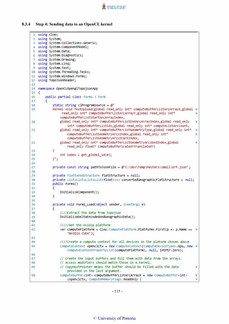
- 115 -

8.3.4 Step 4: Sending data to an OpenCL kernel

- 116 -

- 117 -

- 118 -

Figure 66 - Uploading data to OpenCL

OpenCL is a very complex library and a full discussion of all its intricacies is outside of this scope. This section

is aimed at getting data from a TopoJSON format into the GPU so that a kernel program can be used to assemble

the topology via the GPU. For a brief introduction to OpenCL we will discuss the code in Figure 66. The

application can be subdivided into three main sections:

• The OpenCL kernel.

• Initialising the OpenCL environment.

• Uploading, building and compiling in OpenCL.

8.3.4.1 The OpenCL Kernel

Line 18 to 25 defines the OpenCL kernel as a string and assigns it to the string variable clProgramSource. A

kernel is a function declared in a program and executed on an OpenCL device (Munshi, 2011, p. 16). A kernel

can be identified by the __kernel or kernel qualifier applied to any function defined in a program.

A kernel can take one or more arguments, “global” means that the buffers will be allocated on the largest but

slowest chunk of memory available to the compute device. Data stored in this memory region is visible to all

work items (Banger & Bhattacharyya, 2013, p. 53).

Global memory is best used as streaming memory and as such it should be used in continous blocks. The next

modifier is specified as “read_only” which means that data can only be read from and not modified. Should

write access be required for the data from within the OpenCL kernel, to a buffer that can be accessed by the

host program, then a buffer needs to be created and flagged as “write_only”.

The host program is a C# application that initialises the OpenCL context and manages the setup, data transfer

and synchronisation of OpenCL functions. Looking at the rest of the kernel program nothing is happening

except arguments being created for uploading data to the OpenCL function. There is a single function

“get_global_id()” that is used. This function is a built-in function that returns the current index of the work

- 119 -

item. OpenCL executes in parallel so there is no guarantee that the arrays will be accessed in order. The

“get_global_id()” function provides a way of telling the current function instance which array position to

access.

The main purpose of this kernel is to test how long it takes to upload all the required data from the

FlattenedStructure object. This object contains all the TopoJSON data in a number of flat array structures. The

indexes in the arrays plus the XY data provides a way to reconstruct the polygons back from their basic arc

building blocks.

8.3.4.2 Initialising OpenCL

Line 42 gets the ComputePlatform instance. The test laptop contains two graphic cards. The first is a NVIDIA

Quadro 1000M and the second an Intel HD Graphics 4000 compatible card. This means that the laptop

effectively contains three distinct compute devices. Once for each of the two graphic cards and one for the

Intel CPU. Line 42 selects only the NVIDIA profile. It is possible to create an instance of each of the three

devices and have them run concurrently. This is the power of OpenCL. Writing a single kernel in low-level C

means that they are transferable to any device. The code is written into a string because the OpenCL framework

needs to compile the code into a program using the host device. Once a profile has been obtained it can be

used to initialise an OpenCL context. For sharing data with OpenGL the use of P/Invoke is required on the

opengl32.dll library. Low-level access is obtained by calling the wglGetCurrentDC() method. We have not

done this so far in the example. The reason will be explained further on in the discussion.

Line 45 initialises the OpenCL context whereafter a valid context is available for executing additional

functions.

8.3.4.3 Uploading, building and compiling in OpenCL

OpenCL only supports simple types. As such complex structs and classes cannot be sent to the compute buffers.

This means that data has to be flattened into simple arrays. The TopoJSON reader that was created in the

previous section has a method that performs this function.

Line 60 to line 64 creates the compute buffers that will be used to upload the data from the flat array structures.

The data is not yet being transferred here. The way the function on these lines is being called, causes OpenCL

to create a pointer to the memory location where the buffers will be stored and allocates the memory of the

specified size.

Line 67 creates a ComputeProgram which takes the OpenCL context that was previously created and the kernel

source code as arguments. Line 68 compiles and links a program executable from the supplied source code. If

there is a problem with the kernel, this step will fail. There are methods available for returning the compilation

errors to help with debugging.

- 120 -

At this stage we have a compile program with a single function contained in it. To access the method we need

to create an instance of a ComputeKernel that returns a pointer to the OpenCL function (line 70). Line 71 to

line 82 is mapping the ComputeBuffer objects to the function arguments of the created kernel. We still have

not uploaded the data. OpenCL provides different methods to block execution and to perform synchronisation.

This can be accomplished by using a ComputeEventList which provides for finer grained control or by the use

of the ComputeCommandQueue which provides the finish method. Both methods are illustrated but the

ComputeEventList is commented out on line 99. In this example the active blocking mechanism is using the

ComputeCommandQueue.Finish() method. Line 94 is performing the actual data upload of only one of the

nine required data functions. Line 96 starts the OpenCL execution which blocks on line 102 until the whole

buffer has been uploaded and each of the items have been iterated.

The foreach loop on line 107 to line 122 returns timing information from the executed kernel.

8.4 Results

To upload the data and iterate through each of the items using only one of the nine buffers that would be

required in order to construct the polygons takes less than a 1/1000 of a second. This is really fast even

considering no computations are being executed by the kernel.

The reason a full polygon reconstruction kernel was not implemented was due to a single problem. The time

it takes to convert the TopoJSON file into a flattened structure that can be consumed by OpenCL. It takes

longer to process the TopoJSON file into a flat structure that can be sent to OpenCL than to simply use the

actual created objects, processing them on the CPU and then uploading them directly to OpenGL. It is thus

more efficient to use the CPU to create polygon objects and upload them directly to OpenGL. Looking at the

results and after further study on OpenCL, the polygon construction will be faster on the GPU. The problem

for another research paper is how to efficiently convert the TopoJSON structure into a simple structure that

can be utilised by OpenCL.

So in conclusion this specific implementation and experiment did not provide a speedup with the end goal to

draw a topology in a faster more efficient manner which would enable larger datasets to reside in GPU memory.

- 121 -

9 CONCLUSION AND CLOSING REMARKS

In this dissertation we have looked at a number of different drawing libraries. The main goal of determining if

2D rendering on OpenGL would be a viable solution has been answered to the best of the author’s ability. The

number of experiments completed using different APIs and compared to OpenGL prove that OpenGL provides

a faster more fluid rendering of geographic data.

The technical overhead of learning to use OpenGL properly is worth the result. Building a fully functional GIS

rendering engine with all the required functionality is a monumental task. A task that would require many

programming hours, utilising a large development team. For companies that specialise in building GIS

rendering software, OpenGL should be strongly considered. If the desire is to create a new rendering engine

from scratch, which will be able to make use of future improvements continually being applied to the new

GPUs being developed, OpenGL should be the first choice.

As part of the study into graphics which utilise dedicated graphic hardware the next logical step was to

investigate OpenCL. To get the maximum speed benefit from OpenGL, all geometry data should reside in GPU

memory. An attempt was made to use OpenCL to decode a data format that provides compression. The findings

here were slightly disappointing. Although OpenCL could potentially be very useful for a GIS environment, it

is very difficult to map the problem space to one that is computable via an OpenCL kernel.

The TopoJSON format was investigated due to the massive compression it lends to a dataset. Smaller datasets

means faster data transfers to GPU memory as well as allowing the storage of larger datasets. The GPU could

then decompress the data into the required polygon data. Unfortunately converting the data into a format that

OpenCL could use required a very high upfront CPU investment, making it unfeasible to get the data to

OpenCL where further processing could happen.

Areas of future study could be focused on implementing GIS graphics via OpenGL/OpenCL interopt as well

as computation geometry using the GPU.

In conclusion OpenGL is a viable and effective rendering engine for the creation of 2D GIS graphics. The large

community available and the massive amounts of literature at hand make it possible for anyone interested in

learning how to use OpenGL to become familiar and effective at using it. A large amount of time went into

learning different rendering APIs as well as implementing a number of experimental renderers. All of the

source code is available (see appendix A). The created rendering engine was compared to existing GIS

applications such as MapWindow and QGIS. The OpenGL renderer outperformed the applications by a fairly

large margin. In addition to the available source code there are also some video recordings taken that show the

difference in the rendering performance.

- 122 -

10 REFERENCES AND BIBLIOGRAPHY

3Dlabs Inc. (2005). glEnableVertexAttribArray. Retrieved from Khronos:

http://www.khronos.org/opengles/sdk/docs/man/xhtml/glEnableVertexAttribArray.xml

AAG. (2014, January 1). GIS For Beginners. Retrieved from Association of American Geographers:

http://www.aag.org/galleries/mycoe-files/OT3_GIS_for_beginners.pdf

Adobe Hardware Performance White Paper. (2012). Optimizing Hardware Systems for Adobe® Premiere®

Pro CS6, After Effects® CS6, SpeedGrade™ CS6, and Photoshop® Extended CS6. San Jose.

Ahn, S. (2013). songho. Retrieved from OpenGL Transformation:

http://www.songho.ca/opengl/gl_transform.html

AMD. (2011). http://www.amd.com/. Retrieved November 18, 2013, from

http://www.amd.com/us/documents/49521_graphics101_book.pdf

Apple. (2013, 07 23). OpenGL Programming Guide For Mac. Retrieved from Apple Inc:

https://developer.apple.com/library/mac/documentation/graphicsimaging/conceptual/opengl-

macprogguide/OpenGLProg_MacOSX.pdf

ATTO. (2014). Disk Benchmark. Retrieved from ATTO: http://www.attotech.com/disk-benchmark/

Banger, R., & Bhattacharyya, K. (2013). OpenCL Programming by Example. Birmingham: Packt Publishing.

Blythe, D. (2008). Rise of the Graphics Processor. IEEE, 761-778.

Bostock, M. (2013). GitHub - topojson. Retrieved 08 27, 2013, from

https://github.com/mbostock/topojson/wiki/Specification

Bourgie, M. (2014, January 24). http://www.hardware-revolution.com/best-ssd-best-hard-drive-january-

2014/. Retrieved from Hardware Revolution: http://www.hardware-revolution.com/best-ssd-best-

hard-drive-january-2014/

Buckey, D. J. (2014, January 1). NISL - Eclological Informatics. Retrieved from GIS Introduction:

http://planet.botany.uwc.ac.za/NISL/GIS/GIS_primer/page_12.htm

Bucur, A. (2013). OpenCL - OpenGL ES interop: processing live video streams on mobile devices - case

study. ACM Digital Library.

Butler, H., Daly, M., Doyle, A., Gillies, S., Schaub, T., & Schmidt, C. (2008). The GeoJSON Format

Specification. Retrieved 8 24, 2013, from http://www.geojson.org/geojson-spec.html

Cady, F., Zhuang, Y., & Harchol-Balter, M. (2011). A Stochastic Analysis of Hard Disk Drives. International

Journal of Stochastic Analysis, 1-21.

Cay, T., F., I., & S., D. S. (2004). The Cost Analysis of Satellite Images for Using in Gis by The Pert.

INTERNATIONAL ARCHIVES OF PHOTOGRAMMETRY, 358-363.

Cockburn, A. (2004). Revisiting 2D vs 3D Implications on Spatial Memory. Australian Computer Society,

28, 25-31.

- 123 -

Coetzee, S., & Eksteen, S. (2012). Tertiary education institutions in Africa: Cloudy with a chance of GISc

education in some countries. South African Journal of Geomatics, 1(2), 119-132.

Das, A. (2011). Process Time Comparison between GPU and CPU. Hamburg: Universität Hamburg.

Dell. (2011, May). Solid State Drive vs. Hard Disk Drdive Price and Performance Study. Retrieved from

Dell:

http://www.dell.com/downloads/global/products/pvaul/en/ssd_vs_hdd_price_and_performance_stud

y.pdf

Egbert, S., & Dunbar, M. (2007). Datums - Why One Should Care. Geneva: University of Kansas.

ESRI. (2004). ArcGIS® 9 - Understanding Map Projections. New York.

ESRI. (2012, July). What is GIS? Retrieved from esri.com:

http://www.esri.com/~/media/c371f47805c345fa84d32ac8a675046e.pdf

ESRI. (2013). ArcGIS Resource Center. Retrieved November 21, 2013, from

http://help.arcgis.com/en/arcgisdesktop/10.0/help/index.html#//00sq0000000w000000.htm

Esri. (2014, January 13). Creating a feature class. Retrieved from USDA NRCS National Cartography and

Geospatial Center: ftp://ftp-fc.sc.egov.usda.gov/GIS/applications/CreateFeatureClass.pdf

Guney, C., Yuksel, B., & Celik, R. N. (2004). GIS DATA MODELING OF 17TH CENTURY FORTRESSES

ON DARDANELLES. 12th Int. Conf. on Geoinformatics (pp. 233-240). Gävle: University of Gavle.

Harris, J. W., & Stocker, H. (1998). Handbook of Mathematics and Computational Science. New York:

Springer-Verlag.

Intel. (2010). Intel. Retrieved from Intel® Q67 Express Chipset:

http://www.intel.com/content/www/us/en/chipsets/mainstream-chipsets/q67-express-chipset.html

Internet Engineering Task Force. (2012). A JSON Media Type for Describing the Structure and Meaning of

JSON. Retrieved 8 24, 2013, from http://tools.ietf.org/html/draft-zyp-json-schema-03

Jebara, B. K. (2007). The role of geographic information system (GIS) in the control and prevention of

animal diseases. World Organisation for animal health (OIE), 175-183.

Jones, W. (2004). Beginning DirectX 9. Boston.

Kesteloot, L. (2006, 6 August). Homogeneous Coordinates. Retrieved from Teamten:

http://www.teamten.com/lawrence/graphics/homogeneous/

KHRONOS™ GROUP. (2013). OpenGL. Retrieved November 18, 2013, from

http://www.khronos.org/opengl/

Kilgard, M. J., & Bolz, J. (2012). GPU-accelerated path rendering. ACM Transactions on Graphics (TOG) -

Proceedings of ACM SIGGRAPH Asia 2012, 31(6), Article No. 172 .

Kinsella, J. (2005). The Impact of Disk Fragmentation. Retrieved from Diskeeper:

http://files.diskeeper.com/pdf/impactofdiskfragmentation.pdf

Lantzy, C. R. (2007). Cortical Visual Impairment: An Approach to Assessment and Intervention. New York:

AFB Press.

- 124 -

Lee, V. W., Kim, C., Chhugani, J., Deisher, M., Kim, D., Nguyen, A. D., . . . Dubey, P. (2010). Debunking the

100X GPU vs. CPU Myth: An Evaluation of Throughput Computing on CPU and GPU. Saint-Malo:

ISCA.

Leurs, L. (2014, January 28). RAID. Retrieved from Prepressure.com:

http://www.prepressure.com/library/technology/raid

Lippman, S. B., Lajoie, J., & Moo, B. E. (2013). C++ Primer, Fith Edition. Massachusetts: Objectwrite Inc.

Longley, P. A., Goodchild, M. F., & Rhind, D. W. (2003). Geographic Infromation Systems and Science.

West Sussex: John WIley & Sons.

Luten, E. (2007). What is OpenGL? Retrieved from OpenGLBook: http://openglbook.com/the-book/preface-

what-is-opengl/

Lyons, C. (2010). Video Games: Evolving from a Simple Pastime to One of the Most Influential Industries in

the World. Undergraduate Research Journal at UCCS, 3(1), 10-17.

Mankari, M. P., Kodge, B. G., Kulkarni, M. J., & Nagargoje, A. U. (2010). Fundamentals of geoinformatics

and its applications in geography. Geoscience Research, 1(1), 1-6.

Marsh, M., Hummel, J., Barthelemy, P., Heck, M., & Lichau, D. (2011). Visualisation Sciences Group.

Retrieved from

http://www.vsg3d.com/sites/default/files/related/vsg_hardware_recommendation_for_avizo.pdf

Mcclanahan, C. (2010). History and Evolution of GPU Architecture. Retrieved from

http://mcclanahoochie.com/blog/2011/03/the-history-and-evolution-of-gpu-hardware/

McClure, W. B., Bowling, M., Dunn, C., Hardy, C., & Blyth, R. (2010). Professional iPhone® Programming

with MonoTouch and .NET/C# (1st ed.). Wrox.

Micron Technology. (2014, January 29). Crucial. Retrieved from Memory Speeds and compatibility:

http://www.crucial.com/support/memory_speeds.aspx

Microsoft. (2012, March 7). About Direct2D. Retrieved from Windows Desktop Development:

http://msdn.microsoft.com/en-us/library/windows/desktop/dd370987%28v=vs.85%29.aspx

Microsoft. (2014, February 08). Microsoft Developer Network. Retrieved from Eception.StackTrace

Property: http://msdn.microsoft.com/en-us/library/system.exception.stacktrace(v=vs.110).aspx

Microsoft. (2014, February 8). Microsoft Developer Network. Retrieved from Reflection in the .NET

Framework: http://msdn.microsoft.com/en-us/library/f7ykdhsy(v=vs.110).aspx

Microsoft. (2014). Support is ending soon. Retrieved from Windows: http://windows.microsoft.com/en-

ZA/windows/end-support-help

Mileff, P., & Dudra, J. (2012). Modern Software Rendering. Production Systems and Information

Engineering, 55-66.

Minar, N. (2013). TopoJSON - A smaller GeoJSON with some neat tricks. San Francisco. Retrieved 08 26,

2013, from http://www.somebits.com/~nelson/SotM-2013-TopoJSON.pdf

- 125 -

Munshi, A. (2011, 12 14). The OpenCL Specification V1.2. Retrieved from Khronos Group:

https://www.khronos.org/registry/cl/specs/opencl-1.2.pdf

Neteler, M., & Mitasova, H. (2008). Open Source GIS. New York: Springer Science+Business Media, LLC.

Ogoerg, J. (2012). Songho. Retrieved from MathML Conversion:

http://www.songho.ca/opengl/gl_projectionmatrix_mathml.html

OGP. (2008, August 22). International Association of Oil & Gas Producers. Retrieved from Surveying &

Positioning Guidance Note I: http://www.ogp.org.uk/pubs/373-01.pdf

OGP. (2009, January). International Association of Oil & Gas Producers. Retrieved from Surveying &

Positioning Guidance note 5: http://www.ogp.org.uk/pubs/373-05.pdf

OGP. (2012, August). International Association of Oil & Gas Producers. Retrieved from Using the EPSG

Geodetic Parameter Dataset: http://www.epsg.org/guides/docs/G7-1.pdf

OpenLayers. (2008). Spherical Mercator. Retrieved from OpenLayers:

http://docs.openlayers.org/library/spherical_mercator.html

OpenTK. (2008, August). Retrieved from Building a Windows.Forms + GLControl based application:

http://www.opentk.com/doc/chapter/2/glcontrol

OpenTK. (2014, February 10). Retrieved from The Open Toolkit Manual: http://www.opentk.com/doc

Patterson, D. (2012). Technical Perspective - For Better or worse, benchmarks shape a field. ACM, 104.

Perkins, B. (2012, August 25). Computerworld. Retrieved from 2010:

http://www.computerworld.com/s/article/350588/Have_You_Mapped_Your_Data_Today_

Redden, E. S., Harris, W., Miller, D., & Turner, D. D. (2012, September). Cognitive Load Study Using

Increasingly Immersive Levels of Map-based Information Portrayal on the End User Device. Army

Research Laboratory.

Renhart, Y. (2009). Fast Map Rendering for Mobile Devices. Gothenburg: GUPEA.

Richard, N. G. (2002, November 15). Microsoft Windows' Graphics Device Interface (GDI). Retrieved from

Oregon State University (OSU):

http://classes.engr.oregonstate.edu/eecs/spring2003/ece44x/groups/g1/WhitePaperRichard.pdf

Samsung. (2013, May 13). Samsung SSD 840 PRO Series. Retrieved from Samsung:

http://www.samsung.com/us/pdf/memory-storage/840PRO_25_SATA_III_Spec.pdf

Schildt, H. (2003). Chapter 5 - Pointers. In H. Schildt, The Complete Reference: C++. Fourth Edition (pp.

113 - 154). The McGraw-Hill Companies.

Schildt, H. (2003). The Complete Reference: C++, Fourth Edition. The McGraw-Hill Companies.

Schmandt, M. (2014, January 13). Map Processing. Retrieved from GIS Commons:

http://giscommons.org/earth-and-map-preprocessing/

Schobesberger, D., & Patterson, T. (2008). Evaluating the Effectiveness of 2D vs. 3D Trailhead Maps. Lenk,

Switzerland: In Proceedings of the 6th ICA Mountain Cartography Workshop.

- 126 -

Segal, M., & Akeley, K. (2003). The OpenGL Graphics System: A specification (Version 1.5). Silicon

Graphics, Inc.

Segal, M., & Akeley, K. (2004). The OpenGL Graphics System: A specification (Version 2.0). Silicon

Graphics, Inc.

Segal, M., & Akeley, K. (2006, July 30). OpenGL. Retrieved from The OpenGL Graphics System: A

specification: http://www.opengl.org/documentation/specs/version2.1/glspec21.pdf

Serial ATA Revision 3.0 Specification. (2009, June 2). Serial ATA International Organization: Serial ATA

Revision 3.0. Retrieved from

http://www.lttconn.com/res/lttconn/pdres/201005/20100521170123066.pdf

Shreiner, D., Sellers, G., Kessenich, J. M., & Licea-Kane, B. M. (2013). OpenGL Programming Guide, 8th

Edition. Addison-Wesley.

The Gaia-SINS federated projects. (n.d.). A quick introduction to SpatiaLite Topology. Retrieved 03 06,

2013, from http://www.gaia-gis.it/gaia-sins/topology-preview.pdf

The Khronos Group. (2013). OpenGL Overview. Retrieved from OpenGL: http://www.opengl.org/about/

Tory, M., & Moller, T. (2004). Human factors in Visualisation research. Visualisation and Computer

Graphics, IEEE Transactions, 10(1), 72-84.

United States Geological Survey. (2014, 01 12). United States Geological Survey. Retrieved from USGS:

http://woodshole.er.usgs.gov/project-pages/longislandsound/data/GIS.htm

van Sickle, J. (2010). Basic GIS Coordinates. CRC Press.

Walbourn, C. (2009, August 2012). Graphics APIs in Windows. Retrieved from

https://groups.google.com/forum/#!msg/gpu_newbies/BP5GCXLo8hI/-aIYwBgjkPYJ

Wallossek, I. (2010, February 2010). 2D, Acceleration, And Windows: Aren't All Graphics Cards Equal?

Retrieved from Tomshardware: http://www.tomshardware.com/reviews/2d-windows-gdi,2547.html

Wang, D. T. (2005). MODERN DRAM MEMORY SYSTEMS: PERFORMANCE ANALYSIS AND

SCHEDULING ALGORITHM. Maryland: University of Maryland.

Western Digital. (2014). WD Black. Retrieved from Western Digital:

http://wd.com/en/products/products.aspx?id=760

Wolfram MathWorld. (2014). Tessellation. Retrieved from Wolfram MathWorld:

http://mathworld.wolfram.com/Tessellation.html

Xie, Z., Ye, Z., & Wu, L. (2008). A Design for Polygon Overlay Algorithm in the Simple Feature Model.

Grid and Cooperative Computing, 2008. GCC '08. Seventh International Conference, 680-685.

Zhang, X. (2001). Application-Specific Benchmarking. Cambridge: Harvard University.

Zhu, Q., & Luo, C. (2011). Primary investigation of the 3d GIS based on OpenGL_ES. Multimedia

Technology (ICMT), 2011 International Conference, 5453 -5456.

Zins, C. (2007). Conceptual approaches for defining data, information, and knowledge. Journal of the

American Society for Information Science and Technology, 58(4), 479-493.

- 127 -

11 APPENDIX A - SOURCE CODE AND PROJECT INFORMATION

All the source code that has been used for experimentation and testing is available from

https://41.185.23.90/masters/index.html. A CD containing the source code is also provided with the

dissertation.

In order to make it easier for non-technical people, precompiled libraries and screencasts are available. There

are three main Visual Studio solutions that contain all the experiments and code. Each solution consists of a

number of different libraries and executables. This section will discuss each solution as well as how to execute

each of the programs. For each program the following will be made available:

• An explanation of the function of the program.

• The source code.

• A pre-compiled executable.

• A screencast showing its execution.

11.1 API benchmarking application

The main solution file is called “Benchmarking.sln” and consists of five main applications. If Visual Studio

2012 is available you can download the source code (https://41.185.23.90/masters/sourcecode.zip) and open

the Benchmarking.sln file. Visual Studio should open and load the solution. The solution requires OpenGL

drivers to be installed as well as DirectX. Without the required libraries the solution will not compile.

Depending on the version of Windows a “Loader Lock Exception” might occur while executing the

application. As such it might be a good idea to disable this check in Visual Studio. To do this, while in Visual

Studio press Ctrl + Alt + e. The exceptions dialog should open. On the right hand side of the dialog click on

find and search for ‘LoaderLock’. It will highlight the found item. Uncheck the thrown checkbox and click

OK. See Figure 67.

- 128 -

Figure 67 - Disable LoaderLock Exception

Once this has been disabled, right-click on the solution and click “Build Solution”. The solution should build

without any exceptions. It may be necessary to rebuild once or twice to get all the projects to compile correctly.

In Visual Studio set the desired project as the start-up project and run the application.

A short discussion is to follow on each of the applications by executing them from the precompiled libraries.

11.1.1 GUI.BenchmarkingApp

Navigate into the binaries/benchmarking folder. Double click on the “GUI.BenchmarkingApp.exe”. The main

application windows should open without any exceptions and look like Figure 68

- 129 -

Figure 68 - Gui.BenchmarkingApp Main Form

The radio button on the left denotes the rendering API that is currently enabled. The buttons to the left load the

selected dataset into memory. Once that has completed, the corresponding draw command can be used to

render the data using the selected API. To the right of that is an “Autobenchmark” checkbox. Checking this

box and setting the number of repetitions will make the application run each rendering API with each type of

data for the set number of times. All the executions are logged to a text file contained in the executable directory

called “Benchmark.txt”. Clicking the “Clear Log File” button will clear the log. The “Open Log File” button

will display the log file in the default *.txt editor. A video of the application is viewable by downloading the

screencasts (https://41.185.23.90/masters/Videos.zip). To create the graphs used in this dissertation, the text

file was copied to excel and then graphed.

11.1.2 Console Application Benchmarks - ADO.NET SQLite Benchmark

This application can be found in the “Benchmarking.sln” project under “consoleADOSQLiteBench” or

executed via the command line from the source/binaries folder. This application loads data from SQLite using

the SpatiaLite extension which enables the storage of spatial data. The main purpose of this application is to

measure the time it takes to query a table, return the data and convert the geometry data to a SpatiaLite binary

array.

Command line arguments of the application are as follows:

- 130 -

consoleADOSQLiteBench.exe <path to SQLite database> <number of times to execute the benchmark> <the

name of the table to query>

The result of the benchmark is written to the console. The times indicate how long it takes to iterate 100,000

records.

11.1.3 Console Application Benchmarks - ADO.NET SQLite Benchmark using custom ADO.NET

wrapper

This application is similar to the one above. The main difference is that the ADO.NET provider has been

wrapped in a custom API to allow easier use of ADO.NET.


consoleCustomADOSQLiteBench.exe <path to SQLite database> <number of times to execute the

benchmark> <the name of the table to query>


records. One can view a screencast of the application in the videos folder. As there is another layer of

abstraction, slightly longer execution times are expected.

11.1.4 Console Application Benchmarks - ADO.NET SQLite Benchmark using ADO.NET and a .NET

list

This application loads data from a SQLite database and then stores the data in a list. The data is converted into

a GeoAPI.IGeometry object which is a more useful format. Two metrics are measured. The first is the time to

convert the SQLite binary to GeoAPI.IGeometry objects and store it to a list in memory. The second is the

time it takes to iterate the list of IGeometry objects.


consoleCustomADOWithList.exe <path to SQLite database> <number of times to execute the benchmark>

<the name of the table to query>


records. A screencast of the application can be found in the video folderE:\Library\Mail

Downloads\Source\Videos\consoleCustomADOWithList.mp4.

11.1.5 Console Application Benchmarks - ADO.NET SQLite Benchmark using ADO.NET and a .NET

list

This application uses an ESRI shapefile as its input. It reads the data in the form of a shape object and iterates

through each of the records. The same dataset that was used above was exported to a shapefile and used to run

the tests.

- 131 -


consoleShapefileReaderBench.exe <path to shapefile database> <number of times to execute the benchmark>


records. A screencast of the application can be found in the videos folder

11.1.6 Summary

The purpose of this solution was to benchmark different graphic APIs. The point of the console applications

were to determine what format the data should be served up as in attempting to saturate the graphic rendering

pipeline.

The findings in the end led to all data being cached in main memory and served to the APIs directly from this

location. This ensured that bottlenecks would not be the result of different file formats or storage media which

turned out to be the case. Using this method it was possible to saturate the other graphic APIs with data.

11.2 NetGIS - Points of interest rendering application with zoom and pan

The main solution file for this application is called “NetGIS.sln”. If Visual Studio 2012 is available you can

open the solution file from the src\NetGroupCL folderE:\Library\Mail

Downloads\Source\src\NetGroupCL\NetGIS.sln. Visual Studio should open and load the solution. The

solution requires OpenGL drivers to be installed. This application demonstrates real time rendering of 100,000

points of interest using a custom built OpenGL rendering engine. You can run the application from the

precompiled binary found in the src folder. Double click on the “NetGIS.exe” to start the application. An

application window will open like the one below in Figure 69.

Figure 69 - NetGIS Application

- 132 -

This is a very basic application that allows the viewing of a number of points of interest which are being

rendered in real-time via OpenGL. Real-time rendering means that the entire image is redrawn on every

refresh. The methods used by MapWindow and QGIS are slightly different. They render to a bitmap and only

redraw the new part that has changed or become visible. This should really highlight the speed OpenGL

provides.

To see a screencast of the running application look in the videos folder. For a comparison running against

MapWindow see the NetGIS vs Mapwindow mp4E:\Library\Mail Downloads\Source\Videos\NetGIS vs

MapWindow.mp4. QGIS vs NetGIS is also avilable. QGIS is capable of higher rendering rates than

MapWindow is able to produce but it is still slower than NetGIS which uses OpenGL. QGIS uses the bitmap

rendering trick to speed up drawing as can be seen when panning to the left and then to the right again. A

redraw is only triggered when releasing the mouse button.

11.3 TopoJSON - Rendering using OpenGL/OpenCL

The main solution file for this application is called “TopoJSON.sln”. The solution requires OpenGL/OpenCL

drivers to be installed. There are a number of applications in this solution all based around JSON, OpenCL and

OpenGL. The main projects are the “TopoJsonDrawing”, “TopoJasonReader” and the

“OpenCLOpenglTopojsonApp”. “TopoJsonDrawing” is concerned with drawing a polygon layer using

OpenGL with a vertex buffer object reading from a TopoJSON file. “OpenCLOpenglTopojsonApp” is

concerned with converting the TopoJSON file to a flat structure and benchmarking the time it takes to upload

it to the GPU using OpenCL. “TopoJasonReader” is the main library that was developed to read TopoJSON

files. The application can be executed from the precompiled library under the TopoJSON folder. Double click

on the “TopoJsonDrawing.exe” to start the application. This application simply converts the TopoJSON file

into polygons via the CPU and sends them to OpenGL for rendering. This turned out to be more efficient than

trying to convert the data into a format usable by OpenCL.

For the other projects feel free to peruse the source code. When executing “TopoJsonDrawing.exe” just have

a bit of patience. It will take a little while to recompile the polygon geometries and in the end the screen

depicted in Figure 70 will be displayed.

- 133 -

Figure 70 - TopoJSON Application

For a screencast demonstrating the running application see videos E:\Library\Mail

Downloads\Source\Videos\TopoJSON.mp4. This is a very basic application which was aimed at experimenting

with OpenCL. From this solution it became apparent that the overhead of converting the data into a format that

OpenCL could utilise was higher than simply using the data natively with OpenGL. As such no further

investigation was performed.

Assessing OpenGL for 2D rendering of geospatial data

Documents

Transcript of Assessing OpenGL for 2D rendering of geospatial data