ANL-WIS-PA-000001, Rev. 02, "EBS Radionuclide Transport ...
290
EBS Radionuclide Transport Abstraction 7. VALIDATION Model validation for the EBS Radionueclide TransportAbstraction was performed in accordance with LP-2.29Q-BSC, Planning for Science Activities, and LP-SIII. I OQ-BSC, Models, and follows the validation guidelines in the Technical Work Plan for: Near-Field Environment and Transport: Engineered Barrier System: Radionuclide Transport Abstraction Model Report Integration (BSC 2005 [DIRS 173617]). LP-SIII.IOQ-BSC, Models, requires that TSPA-LA model components be validated for their intended purpose and stated limitations, and to the level of confidence required by the relative importance of the component to the potential performance of the repository system. Three levels of model validation are defined in LP-2.29Q-BSC, Planning for Science Activities, Attachment 3, with the level of validation increasing with an increasing level of model importance ranging from low to moderate to high. Models whose variation could lead to a potentially large effect on the estimate of mean annual dose (e.g., a change greater than 1 mrem yr-) should receive a high or Level III model validation. Models whose variation could lead to moderate effect on the estimate of mean annual dose (less than I mrem yr-, but greater than 0.1 mrem yF') should receive Level II model validation. Level I validation is sufficient for models of less importance to the estimate of mean annual dose. The levels of confidence required for the models of the EBS RT Abstraction, as stated in Section 2.2.2 of the TWP, are given as follows. The required level of confidence for the EBS flow model is Level I. The required level of confidence for the EBS transport model is Level II. The required level of confidence for radionuclide transport from the waste package to the drift wall through the invert is Level I (also specified in Table I of LP-2.29Q-BSC, Planning for Science Activities). The EBS-UZ interface model of the EBS RT Abstraction provides input to the unsaturated zone radionuclide transport model as described in Particle Tracking Model and Abstraction of Transport Processes (BSC 2004 [DIRS 170041]). The appropriate level of confidence identified for unsaturated zone radionuclide transport is Level II. Therefore, Level II also represents appropriate level of confidence for the EBS-UZ interface model of the EBSRTAbstraction. Confidence Building During Model Development to Establish Scientific Basis and Accuracy for Intended Use For Level I validation, Section 2.2.3 of the TWP (BSC 2005 [DIRS 173617]) cites Attachment 3 of LP-2.29Q-BSC as guidance for documenting a discussion of decisions and activities for confidence building during model development. Additionally, the development of the model will be documented in accordance with the requirements of Section 5.3.2(b) of LP-S1II.IOQ-BSC. The development of the EBS RT Abstraction model has been conducted according to these requirements and the requisite criteria have been met as discussed below: 1. Selection of input parameters and/or input data, and a discussion of how the selection process builds confidence in the model [LP-SIII.IOQ-BSC 5.3.2(b) (1) and LP-2.29Q-BSCAttachmnent 3 Level l (a)]. ANL-WIS-PA-000001 REV 02 7-1 August 2005
-
Upload
khangminh22 -
Category
Documents
-
view
0 -
download
0
Transcript of ANL-WIS-PA-000001, Rev. 02, "EBS Radionuclide Transport ...
EBS Radionuclide Transport Abstraction
7. VALIDATION
Model validation for the EBS Radionueclide Transport Abstraction was performed in accordancewith LP-2.29Q-BSC, Planning for Science Activities, and LP-SIII. I OQ-BSC, Models, andfollows the validation guidelines in the Technical Work Plan for: Near-Field Environment andTransport: Engineered Barrier System: Radionuclide Transport Abstraction Model ReportIntegration (BSC 2005 [DIRS 173617]).
LP-SIII.IOQ-BSC, Models, requires that TSPA-LA model components be validated for theirintended purpose and stated limitations, and to the level of confidence required by the relativeimportance of the component to the potential performance of the repository system. Three levelsof model validation are defined in LP-2.29Q-BSC, Planning for Science Activities,Attachment 3, with the level of validation increasing with an increasing level of modelimportance ranging from low to moderate to high. Models whose variation could lead to apotentially large effect on the estimate of mean annual dose (e.g., a change greaterthan 1 mrem yr-) should receive a high or Level III model validation. Models whose variationcould lead to moderate effect on the estimate of mean annual dose (less than I mrem yr-, butgreater than 0.1 mrem yF') should receive Level II model validation. Level I validation issufficient for models of less importance to the estimate of mean annual dose.
The levels of confidence required for the models of the EBS RT Abstraction, as stated inSection 2.2.2 of the TWP, are given as follows.
The required level of confidence for the EBS flow model is Level I. The required level ofconfidence for the EBS transport model is Level II. The required level of confidence forradionuclide transport from the waste package to the drift wall through the invert is Level I (alsospecified in Table I of LP-2.29Q-BSC, Planning for Science Activities). The EBS-UZ interfacemodel of the EBS RT Abstraction provides input to the unsaturated zone radionuclide transportmodel as described in Particle Tracking Model and Abstraction of Transport Processes(BSC 2004 [DIRS 170041]). The appropriate level of confidence identified for unsaturated zoneradionuclide transport is Level II. Therefore, Level II also represents appropriate level ofconfidence for the EBS-UZ interface model of the EBSRTAbstraction.
Confidence Building During Model Development to Establish Scientific Basis andAccuracy for Intended Use
For Level I validation, Section 2.2.3 of the TWP (BSC 2005 [DIRS 173617]) cites Attachment 3of LP-2.29Q-BSC as guidance for documenting a discussion of decisions and activities forconfidence building during model development. Additionally, the development of the modelwill be documented in accordance with the requirements of Section 5.3.2(b) ofLP-S1II.IOQ-BSC. The development of the EBS RT Abstraction model has been conductedaccording to these requirements and the requisite criteria have been met as discussed below:
1. Selection of input parameters and/or input data, and a discussion of how the selectionprocess builds confidence in the model [LP-SIII.IOQ-BSC 5.3.2(b) (1) andLP-2.29Q-BSCAttachmnent 3 Level l (a)].
ANL-WIS-PA-000001 REV 02 7-1 August 2005

EBS Radionuclide Transport Abstraction
The inputs to the EBS RT Abstraction have been obtained from appropriate sources asdescribed in Section 4.1. All the data are qualified project data developed by or for theYucca Mountain Project. Tables 4.1-1 through 4.1-20 describe the input parameters, thevalues of the parameters and the source of the information. Inputs were selected becausethey are expected to represent conditions at the repository and therefore build confidencein the model. Thus, this requirement can be considered satisfied.
2. Description of calibration activities, initial boundary condition runs, run convergences,simulation conditions set up to span the range of intended use and avoid inconsistentoutputs, and a discussion of how the activity or activities build confidence in the model.Inchlsion of a discussion of impacts of any non-convergence runs [(LP-SIII.IOQ-BSC5.3.2(b0)(2) and LP-2.29Q-BSC Attachment 3 Level I (e)].
A detailed discussion of the computational implementation of the EBS RT Abstraction isdescribed in Section 6.5.3. The discretization and development of the computational cellnetwork of the sub-model domains is described in Section 6.5.3.5. Section 6.5.3.6provides special emphasis and discussion of the EBS-UZ boundary condition.Simulation conditions account for both seepage or no seepage boundary conditions andthe flux splitting algorithm accounts for the eight key flow pathways in the engineeredbarrier system. Discussion about non-convergence runs is not relevant for this modelreport. Thus, this requirement can also be considered satisfied.
3. Discussion of the impacts of uncertainties to the model results inchlding how the modelresults represent the range of possible outcomes consistent with important uncertainties[(LP-SIII.JOQ-BSC 5.3.2(b)(3) and LP-2.29Q-BSC Attachment 3 Level I (d) and (/)].
Data uncertainty is addressed in Section 6 and parameter uncertainties are summarizedin Table 6.5-6. In particular, corrosion rates of carbon and stainless steels are listed asmodel input with ranges and distributions determined from the data in Table 4.1-1.Sorption coefficient distribution ranges are summarized in Table 4.1-15 and samplingcorrelations are given in Table 4.1-16. Table 4.1-8 provides uncertainty for unsaturatedzone parameters. The breached drip shield experimental test data in Tables 4.1-2through 4.1-6 and Figure 4.1-1 are evaluated in Section 6.5.1, resulting in uncertainmodel input parameters listed in Table 6.5-6 (FluxSplitDSUncert andFluxSplitWPUncert).
Model uncertainty is addressed through the evaluation of alternative conceptual models.In considering alternative conceptual models for radionuclide release rates and solubilitylimits (Sections 6.4. and 6.6), the EBS radionuclide transport abstraction uses modelsand analyses that are sensitive to the processes modeled for both natural andengineering systems.
Conceptual model uncertainties are defined and documented, and effects onconclusions regarding performance are assessed. The fundamental relationships,e.g., mass balance and flow equations, upon which the EBS RTAbstraction is based, arewell-established with a long history of use in the scientific community and as such arenot subject to significant uncertainty. In addition, the alternative conceptual models havebeen screened out (Section 6.4), thereby increasing confidence in the selected conceptual
ANL-WIS-PA-000001 REV 02 7-2 August 2005

EBS Radionuclide Transport Abstraction
model. Other sources of uncertainty involve modeling choices (e.g., assumptions,geometry) that, because of their conservative nature, effectively bound uncertainty.Therefore this requirement can be considered satisfied.
4. Formulation of defensible assumptions and simplifications [LP-2.29Q-BSC Attachment 3Level I (b)].
A discussion of assumptions is provided in Section 5. The conceptual model for EBS RTAbstraction are documented in Section 6.3.1 and the simplifications necessary forimplementation based on EBS design details and failure mechanisms are presented inSections 6.3.3 and 6.3.4. Thus, this requirement can also be considered satisfied.
5. Consistency with physical principles, such as conservation of mass, energy, andmomentutm [LP-2.29Q-BSC Attachment 3 Level I (c)].
Consistency with physical principles is demonstrated by the development of the massbalance mathematical formulations in Section 6.5.1. Thus, this requirement can also beconsidered satisfied.
Confidence Building After Model Development to Support the Scientific Basis of the Model
Level II validation includes the above Level I criteria and a single post development modelvalidation method described in Paragraph 5.3.2c of LP-SIII.10Q-BSC, Models, consistent with amodel of moderate importance to mean annual dose.
To build further confidence in the EBS RT Abstraction, an independent model validationtechnical review was conducted as specified by the TWP (BSC 2005 [DIRS 173617],Sections 2.2.3 and 2.2.4) for the EBS flow model, the EBS transport model, and the EBS-UZinterface model. This approach is based on requirements of LP-SIII.1OQ-BSC, Section 5.3.2 c),where independent technical review is listed as an appropriate method for model validation.Validation is achieved if the review determines that the questions/criteria for this model, listed inSection 2.2.4 of the TWP, are met. Qualifications of and review tasks to be completed by theindependent technical reviewer are described in Section 2.2.4 of the TWP. The model validationcriteria are described as follows (BSC 2005 [DIRS 173617], Section 2.2.4).
EBS Flow Model Validation Criteria
Criteria that the validation of the EBS flow model is met are as follows. Each shall be confirmedby the independent model validation technical reviewer.
a) The approach and algorithms described in the document and provided to the TSPAcapture all known flow pathways into and from EBS components.
b) Modeling assumptions are clearly defined, discussed, and justified as appropriate for theintended use of the model.
c) Uncertainties in parameters, processes, and assumptions are sufficiently described, andimpacts of these uncertainties discussed.
ANL-WIS-PA-000001 REV 02 7-3 August 2005

EBS Radionuclide Transport Abstraction
d) The overall technical credibility of the approach, including assumptions, parameters,equations, and the TSPA implementation, are sufficient for the model's intended use.
EBS Transport Model Validation Criteria
Criteria that the validation of the EBS transport model is met are as follows. Each shall beconfirmed by the independent model validation technical reviewer.
a) The approach and algorithms described in the document and provided to TSPA addressall known modes of radionuclide transport within and from the EBS components.
b) Modeling assumptions are clearly defined, discussed, and justified as appropriate for theintended use of the model.
c) Uncertainties in parameters, processes, and assumptions are sufficiently described, andimpacts of these uncertainties discussed.
d) The overall technical credibility of the approach, including assumptions, parameters,
equations, and the TSPA implementation, are sufficient for the model's intended use.
EBS-UZ Interface Model Validation Criteria
The criterion that the validation of the EBS-UZ interface model is met shall consist ofconcurrence by an independent technical reviewer that the invert fracture-matrix partitioningresults obtained using this model compare favorably with the fracture-matrix partitioningcumulative distribution function obtained using a discrete fracture model described in theDrift-Scale Radionuclide Transport model (BSC 2004 [DIRS 170040]). Results of thecomparison shall show qualitative agreement between the two methods. The report shalldocument equivalent trends and correlations between input parameter variation and predictedresults, identification of differences between the model results, and a discussion of the reasonsand potential significance of these differences, and shall also demonstrate that the EBS-UZinterface model provided to TSPA does not underestimate radionuclide transport from the EBSto the UZ.
The results of the independent model validation technical review for the flow and transportmodels demonstrate that the appropriate criteria from above have been met, and are presented inSection 7.2.3. The results of the EBS-UZ interface model review demonstrate that theappropriate criteria listed above have been met, and are presented in Section 7.3.2.
The validation guidelines in the TWP (BSC 2005 [DIRS 173617]) also state that the SubjectMatter Expert (author) may elect, as deemed appropriate, to provide additional validation in theform of:
* Corroboration of model results with data previously acquired from laboratoryexperiments or other relevant observations
* Corroboration of model results with results of alternative models
ANL-WIS-PA-000001 REV 02 7-4 August 2005

EBS Radionuclide Transport Abstraction
* Corroboration with information published in refereed journals or literature.
In addition to the independent model validation technical review, the post development modelvalidation for the EBS-UZ interface model, as delineated in the TWP, includes corroboration bycomparison to an alternative mathematical model developed for a closely comparable descriptionof the relevant EBS-UZ features. This validation approach is consistent withParagraph 5.3.2(c)(2) of LP-SIII.l0Q-BSC, Models, which lists corroboration of results withalternative mathematical models as one of the validation methods for Level II validation. Thiscomparison is documented in Section 7.3.1.
Additional validation of the flux splitting portion of the flow model was performed throughcorroboration of model results of experimental data. The results of that validation exercise arepresented in Section 7.1.1.
Additional validation of the in-package diffusion portion of the transport model was performedthrough corroboration with alternative models. The results of that validation exercise arepresented below in Section 7.2.
7.1 EBS FLOW MODEL
The EBS flow is modeled as a one-dimensional, steady advective flow through the componentsof the EBS. The sources of flow to the model include a seepage flux from the roof of the drift,condensation on the walls of the drift above the drift shield, and an imbibition flux from theunsaturated zone into the crushed tuff invert. The output of the flow model includes anadvective flux from the invert into the unsaturated zone.
The conceptual model divides the EBS components into three domains: waste form, wastepackage corrosion products, and the invert. Flow and transport in these domains are treatedseparately. The output of the waste form domain feeds into the corrosion products domain. Theoutput of the corrosion products domain in turn feeds the invert.
The flow through the EBS may occur along eight pathways: (1) total dripping flux (seepageinflow from the crown of the drift plus any condensation that may occur on the walls of the driftabove the drift shield), (2) flux through the drip shield, (3) diversion around the drip shield,(4) flux through the waste package, (5) diversion around the waste package, (6) total flux into theinvert, (7) imbibition flux from the unsaturated zone matrix to the invert, and (8) flux from theinvert to the unsaturated zone fractures.
The magnitude of seepage fluid passing through the drip shield and the waste package isaccounted for using the flux splitting submodel. This submodel determines how much waterflows through the drip shield or waste package and how much is diverted around thesecomponents. Below is the validation of the submodel and validation criteria for both the dripshield and waste package applications. Further discussions relevant to the validation of the flowmodel can be found in Sections 5, 6.3.2, 6.3.3, 6.5.1.1.1, 6.5.1.1.2, and 6.5.1.1.3.
ANL-WIS-PA-000001 REV 02 7-5 August 2005
EBS Radionuclide Transport Abstraction
7.1.1 Flux Splitting Submodel
The EBS flux splitting submodel, which is part of the EBS RT Abstraction flow model,determines the fraction of total dripping flux that will flow through the drip shield and/or wastepackage. This submodel is directly related to the waste isolation attribute (i.e., the limitedrelease of radionuclides from engineered barriers). The amount of water flowing throughengineered barriers, when combined with radionuclide solubility limits and diffusive transport,defines the mass flux of radionuclides that is mobilized for transport through the EBS to theunsaturated zone.
Level I validation is appropriate for the flux splitting submodel, because it is part of the processfor radionuclide transport from waste package to the drift wall through the invert (see Section 7above). In addition, the flux splitting submodel has the following features:
" The submodel is not extrapolated over large distances, spaces or time.
* The submodel has large uncertainties because of the chaotic nature of the flow ofdroplets or rivulets on corroded, roughened surfaces.
" Sensitivity analyses in the prioritization report Risk Information to SupportPrioritization of Performance Assessment Models (BSC 2003 [DIRS 168796],Sections 3.3.6 through 3.3.11) show that the flux splitting abstraction will not have alarge impact on dose in the first 10,000 years.
* The flux splitting submodel plays a minor role in TSPA-LA. In the nominal scenarioclass, neither the drip shield nor the waste package fails due to general corrosion withinthe 10,000-year regulatory period (BSC 2004 [DIRS 169996], Section 7.2); if theTSPA-LA model is run to compute the peak dose, which occurs beyond the 10,000-yearregulatory period, then the flux splitting model will be used in the nominal scenarioclass. When the drip shield does fail (beyond the 10,000-year regulatory period in thenominal scenario class), it is modeled as failing completely in a single time step(BSC 2004 [DIRS 169996], Section 6.3). The early waste package failure modelingcase is part of the nominal scenario class, where the drip shield does not fail withinthe 10,000-year regulatory period; thus, the flux splitting submodel is not used. In theigneous scenario class, neither the drip shield nor the waste package survives an igneousintrusion, so the flux splitting submodel is not used. Stress corrosion cracking of thedrip shield occurs in the seismic scenario class, but since no advective flux is allowedthrough the cracks, the flux splitting submodel is not used. Thus, the flux splittingsubmodel is actually applied only in the seismic scenario class when seismic damageoccurs to the waste package from fault displacement leading to fractional failure of thewaste package.
This flux splitting submodel is validated through comparison to experimental data. A work planentitled Test Plan for: Atlas Breached Waste Package Test and Drip Shield Experiments(BSC 2002 [DIRS 158193]) defines the experiments used for validation of this fluxsplitting submodel.
ANL-WIS-PA-000001 REV 02 7-6 August 2005

EBS Radionuclide Transport Abstraction
The flux splitting submodel is applied to two components of the EBS-the drip shield and thewaste package-and is validated for each. Validation is achieved through comparison of themodels developed in this document (based in part on the qualified experimental data) to otherqualified data collected during associated testing. This comparison is limited because thevalidation experiments are based on flow measurements from a single fixed source for dripping,whereas the abstraction is based on randomly located drips relative to multiple patches on thedrip shield. In this situation, the appropriate criterion for model validation is that the ranges ofpredictions of the abstraction, based on smooth drip shield mock-up surface data, overlap theranges of experimental measurements made on the rough drip shield mock-up surface. Thiscriterion is appropriate because of the large spread of the experimental data.
The rough drip shield surface experiments replicate the smooth drip shield surface experimentsand constitute a consistent set of data that can be compared with and serve as validation for thesmooth drip shield surface data. The rough surface would be expected to yield results(specifically, the flux splitting uncertainty factors) that differ from those obtained for the smoothsurface. However, because the only difference in the experiments is the surface texture, thetrends in the data and the values obtained for the uncertainty factors should be similar, whichvalidates the flux splitting submodel.
Experimental data used to develop the flux splitting submodel include the splashradius, the rivulet spread distance or angle, and the fraction of dripping flux thatflowed into breaches. For the drip shield and waste package flux splitting submodels, data fromsmooth drip shield experiments were used (DTNs: MO0207EBSATBWP.022 [DIRS 163400];MO0207EBSATBWP.023 [DIRS 163402]; MO0207EBSATBWP.024 [DIRS 163401];MO0207EBSATBWP.025 [DIRS 163403]). For validation of the models, data from therough drip shield experiments are used (DTNs: MO0207EBSATBWP.021 [DIRS 163399];MO0208EBSATBWP.027 [DIRS 163404]; MO0208EBSATBWP.028 [DIRS 163405]). Each ofthe types of data used is discussed below, first for the drip shield submodel validation and thenfor the waste package flux splitting submodel validation.
7.1.1.1 Drip Shield Flux Splitting Submodel
Splash radius data for dripping onto the crown of the rough drip shield surface are listed inTable 7.1-1. The data are analyzed in the Microsoft Excel spreadsheet: Flux SplittingValidation, Worksheet: Splash Rad vs Number, which is documented in Appendix E. As shownin Figure 7.1-1, the splash radius tends to increase as the number of drips increases. The innercluster radius is of interest because it is used to define the effective length of the drip shield indeveloping the flux splitting submodel (see Section 6.5.1.1.2). While the data do not indicatethat a maximum splash radius was achieved, it stands to reason that a maximum must exist,simply because the distance a splashed droplet can travel is finite, limited by the kinetic energyof a falling drop. The uncertain parameter in the drip shield flux splitting submodel, fD's, was
based on the maximum splash distance observed for the inner cluster of droplets on a smoothdrip shield, 48 cm (see Section 6.5.1.1.2.4 for a discussion of the development of fs based on
the 48-cm maximum inner cluster splash radius). For the rough drip shield tests, the maximuminner cluster splash radius for dripping onto the crown was again 48 cm. Another approach is touse the splash radius at which rivulets begin to flow from coalesced droplets. In Splash Radius
ANL-WIS-PA-000001 REV 02 7-7 August 2005
EBS Radionuclide Transport Abstraction
Test #1, rivulet flow began after 143 drips; in Test #2, after 145 drips; and in Test #3,after 133 drips (DTN: MO0207EBSATBWP.021 [DIRS 163399]), for an average of 140 drips.Using the Microsoft Excel Trendline application (least squares fitting routine) for the innercluster data in Figure 7.1-1, the splash radius when rivulets began to flow was 31 cm. Theminimum splash radius was about 3.5 cm for more than 20 drips (see Table 7.1-1). The range ofuncertainty is bounded using the extreme values of splash radius (3.5 - 48 cm). Since the valueof splash radius at which rivulets begin to flow (31 cm) is between those extremes, an estimate ofuncertainty based on that value will not affect the estimated bounds on uncertainty.
The flux splitting submodel also depends on the rivulet spread angle. These data are analyzed inthe Microsoft Excel spreadsheet: Flux Splitting Validation, Worksheet: Rough DS, which isdocumented in Appendix E. For the smooth drip shield, the spread angle from crown driplocations ranged from 8.90 to 17.3' (± one standard deviation from the mean of 13.20; seeSection 6.5.1.1.2.4). For drip locations on the crown, the rough drip shield surface had a meanrivulet spread angle of 7.3', with a range of 0' to 14.40 (± one standard deviation from themean). Rivulet spread data for the rough surface are shown in Table 7.1-2. In Table 7.1-4, thespread angle calculation results are shown.
The amount of water dripped onto the crown and water flow into breaches on the rough dripshield surface are listed in Table 7.1-3. The fraction of the dripping flux that flowed into thepertinent breach, f~,,,, is shown along with the rivulet spread angle for each particular test
in Table 7.1-4.
ANL-WIS-PA-000001 REV 02 7-8 August 2005

EBS Radionuclide Transport Abstraction
Table 7.1-1. Atlas Breached Drip Shield Experiments on Rough Drip Shield Surface - Dripping onCrown - Splash Radius Tests
Splash Radius (cm)No. Drips Left I Right Comments
Splash Radius Test #110 2.0 2.0 Measured inner cluster (bulk)10 15.0 25.5 Measured outer fringe21 5.0 4.0 Measured inner cluster (bulk)21 15.0 42.5 Measured outer fringe60 18.0 22.0 Measured inner cluster (bulk)60 72.5 75.5 Measured outer fringe143 35.0 48.0 Measured inner cluster (bulk)143 54.0 82.5 Measured outer fringe203 35.0 48.0 Measured inner cluster (bulk)203 79.5 106.5 Measured outer fringe
Splash Radius Test #2
21 3.5 4.0 Measured inner cluster (bulk)21 37.5 7.0 Measured outer fringe82 10.5 19.0 Measured inner cluster (bulk)82 63.0 32.0 Measured outer fringe149 31.5 30.0 Measured inner cluster (bulk)207 45.0 40.0 Measured inner cluster (bulk)
Splash Radius Test #330 7.5 9.0 Measured inner cluster (bulk)82 19.0 17.5 Measured inner cluster (bulk)137 28.0 27.5 Measured inner cluster (bulk)205 29.0 28.0 Measured inner cluster (bulk)
DTN: MO0207EBSATBWP.021 [DIRS 163399].
ANL-WIS-PA-000001 REV 02 7-9 August 2005

BBS Radionuclide Transport Abstraction
120
100
EU)
0)
a~n* Inner Cluster
q Outer Fringe6O0
0-- Poly. (Outer
Fringe)40 , Poly. (Inner
Cluster)
20
00 50 100 150 200 250
Number of Drips
Figure 7.1-1. Splash Radius Dependence on Number of Drips for Rough Drip Shield Tests
Table 7.1-2. Atlas Breached Drip Shield Experiments on Rough Drip Shield SurfaceCrown - Rivulet Spread Data - 330 from Crown
- Dripping on
RelevantDrip Location Left (cm) Right (cm) Patch
Multiple Patch Tests (DTN: MO0208EBSATBWP.027 [DIRS 163404])
81 cm left of drip shield center 32.5 17.5 4
27 cm left of drip shield center 21.5 18.0 4
27 cm right of drip shield center 10.0 10.0 5
27 cm right of drip shield center 1.0 0 5
81 cm right of drip shield center 17.0 34.0 5
Bounding Flow Rate Tests (DTN: MO0208EBSATBWP.028 [DIRS 163405])
54 cm left of drip shield center (High Flow Rate) 2 0 4
27 cm left of drip shield center (High Flow Rate) 15 15 4
27 cm right of drip shield center (High Flow Rate) 6 6 5
27 cm right of drip shield center (Low Flow Rate) 50.0 16.0 5
27 cm right of drip shield center (Low Flow Rate) - 1.0 5
27 cm left of drip shield center (Low Flow Rate) 25.5 12.0 4
54 cm left of drip shield center (Low Flow Rate) 0 0 4
ANL-WIS-PA-000001 REV 02 7-10 August 2005

EBS Radionuclide Transport Abstraction
Table 7.1-3. Atlas Breached Drip Shield Experiments on Rough Drip Shield Surface - Dripping onCrown - Flow into Breaches
Drip Location Relative to: Water Collected in:Breach B4 Breach B5 Water Breach B4 Breach B5
Drip Location (cm) I (cm) Input (g) (g) (g)Multiple Patch Tests (DTN: MO0208EBSATBWP.027 [DIRS 163404])
81 cm left of drip shield center -27 -135 292.35 0.27 0.0027 cm left of drip shield center 27 -81 288.45 5.27 0.00
27 cm right of drip shield center 81 -27 291.62 0.00 0.0827 cm right of drip shield center 81 -27 294.13 0.00 0.27
81 cm right of drip shield center 135 27 290.10 0.00 1.01Bounding Flow Rate Tests (DTN: MO0208EBSATBWP.028 DIRS 163405])
54 cm left of drip shield center 0 -108 330.74 193.87 0.00(High Flow Rate)
27 cm left of drip shield center 27 -81 328.65 0.63 0.00(High Flow Rate)
27 cm right of drip shield center 81 -27 306.65 0.00 0.35(High Flow Rate)
27 cm right of drip shield center 81 -27 545.14 0.00 11.11(Low Flow Rate)
27 cm right of drip shield center 81 -27 70.80 0.00 0.00(Low Flow Rate)
27 cm left of drip shield center 27 -81 113.32 1.36 0.00(Low Flow Rate) I I I I_1__
54 cm left of drip shield center 0 108 118.10 0.00 0.00(Low Flow Rate) I I I I I _I
Table 7.1-4. Atlas Breached Drip Shield Experiments on Rough Drip Shield Surface - Dripping onCrown - Fraction of Dripping That Flowed into Breaches and Rivulet Spread Angle
Breach Spread An le (degree)
Drip Location Collecting Flow fopt Left Right
81 cm left of drip shield center 4 0.0018 13.4 7.327 cm left of drip shield center 4 0.0365 9.0 7.527 cm right of drip shield center 5 0.0005 6.6 6.6
27 cm right of drip shield center 5 0.0018 0 0.781 cm right of drip shield center 5 0.0070 11.2 21.6
54 cm left of drip shield center 4 1.1723 0.8 0(High Flow Rate)
27 cm left of drip shield center 4 0.0038 6.3 6.3(High Flow Rate)27 cm right of drip shield center (High Flow Rate) 5 0.0023 4.0 4.0
27 cm right of drip shield center 5 0.0408 30.2 10.5(Low Flow Rate)27 cm right of drip shield center 5 0.0110 - 0.7(Low Flow Rate)
ANL-WIS-PA-000001 REV 02 7-11 August 2005

EBS Radionuclide Transport Abstraction
Table 7.1-4. Atlas Breached Drip Shield Experiments on Rough Drip Shield Surface - Dripping onCrown - Fraction of Dripping That Flowed into Breaches and Rivulet Spread Angle(Continued)
Breach Collecting Spread Anole (degree)Drip Location Flow fxpt Left Ri ht
27 cm left of drip shield center (Low Flow Rate) 4 0.0240 10.6 5.054 cm left of drip shield center (Low Flow Rate) 4 0.0 0 0Mean - 0.108 7.25Standard Deviation - 0.335 7.18Median - 0.005 6.29Source: Microsoft Excel spreadsheet: Flux Splitting Validation, Worksheet: Rough DS, documented in
Appendix E.
NOTES: - = no measurement.Mean, standard deviation, and median for spread angle are for all (left and right) measurements.
Following the approach used in Section 6.5.1.1.2.4, the "inner cluster" splash diameter is usedfor the effective length of the drip shield in the validation of the flux splitting algorithm, which isgiven by Equations 6.3.2.4-4 and 6.3.2.4-6 (or 6.5.1.1.2-35). The form of the equation is:
F= Los I + t jana (Eq. 7.1.1.1-1)
where F is the fraction of dripping flux that flows through breaches, t is one-half the width of abreach or patch, LDs is the effective length of the drip shield (i.e., the length over which dripping
or splattering occurs), a is the rivulet spread angle, and f'D is the uncertainty factor for the drip
shield developed for validation, corresponding to the drip shield uncertainty factor, fDs. For thevalidation tests, the number of breaches, Nb, is one.
The splash diameter is used for the effective length, LDs. As shown in Table 7.1-1, the "innercluster" splash radius on the rough drip shield surface ranged from 3.5 cm to 48 cm (for morethan 20 drops), giving a range for LDS of 7 cm to 96 cm. The spread angle ranged (one standard
deviation from the mean) from zero to 14.40. For a drip shield patch width of 27 cm, f =
13.5 cm. Then, as shown in Table 7.1-5, F/f .D= Ný " I + tan -- ranges from 0.141 to 2.17.
LDS of 2ETable 7.1-5. Range of Estimates for FlfvD
Drip ShieldF/fvD
LDs (cm) a = 0° a= 14.4*
7 1.93 2.17
96 0.141 0.158
ANL-WIS-PA-000001 REV 02 7-12 August 2005

EBS Radionuclide Transport Abstraction
The fraction of dripping flux, fLIp,, that entered breaches in 12 rough drip shield experiments
ranged from zero to 1.17, with a mean of 0.108 and a median of 0.0054. The wide range ofuncertainty and randomness in the experiments is demonstrated in two of the tests having thesame drip location (54 cm to the left of the drip shield center). The high drip rate test yielded thehighest flow into a breach with a negligible spread, which is the expected result. What appearsto be an unphysical result for this test, f-,p, = 1.17, is obtained from the assumption that half of
the dripping flux onto the crown flows down each side of the drip shield. This was evidently notthe case in this particular test, since more than half of the dripping flux flowed into the breach.However, since there are no data available to determine what fraction of the dripping flux floweddown the side with the breach, the procedure for calculating fep, is followed without limiting the
values that are obtained (e.g., by limiting fexp, to a maximum of 1.0). The low drip rate test at
the same drip location, which had zero rivulet spread, unexpectedly resulted in no flow into thebreach. Statistics for fLp, are compared in Table 7.1-6 between the smooth drip shield surface
experimental results (Table 6.5-2) and the rough surface results discussed in this section.
Table 7.1-6. Comparison of fexpt Statistics for Smooth and Rough Drip Shield Surfaces
Experiments Mean fexpt Minimum fe.,,t Maximum fept Median fexpt
Drip Shield (Smooth Surface) 0.111 0.013 0.275 0.049
Drip Shield Validation (Rough Surface 0.108 0.0 1.17 0.0054
The rough surface experimental results are now used to calibrate the drip shield flux splittingsubmodel that is developed for validation purposes, yielding the uncertainty factor fvD :
fV= fe xP, (Eq. 7.1.1.1-2)I (,tan o)LDS 2)
f,, is at a minimum using the minimum value for LDs (7 cm) and the maximum value for a
(14.40), resulting in fD = 0.46f,',,. The maximum for fvD is obtained using the maximum
value forLDs (96 cm) and the minimum value fora (00), resulting in f'D =7.If.p,. Using the
mean value for f~p, (0.108) results in a range for fvD of 0.050 to 0.77. The drip shield flux
splitting algorithm developed in Section 6.5.1.1.2.4 produced the corresponding factor fDs
ranging from about 0.36 to 0.73. These factors (f'D and fDs) actually represent the estimates of
the upper bound on the uncertainty, since a lower bound is necessarily zero (i.e., no flow througha breach). Using the actual measured range of fex,, (0.0 to 1.17) instead of the mean increases
the range estimated for fvD to 0.0 to (7.1)(1.17) = 8.3. The corresponding range for fDs, using
the measured range of f,,, (0.013 to 0.275) (Table 6.5-2) for the smooth surface tests instead of
the mean (0.111), is 0.013/0.31 = 0.041 (for LDs =50cm, a = 17.30) to 0.275/0.152 = 1.8 (for
LDs = 96 cm, a = 8.9°). Thus, using the extreme values of fv,, for estimating fDs and fvD, the
ANL-WIS-PA-000001 REV 02 7-13 August 2005

EBS Radionuclide Transport Abstraction
upper bound on fvD actually spans the uncertainty in the upper bound estimate of fDs, assummarized in Table 7.1-7.
Table 7.1-7. Summary of fos and fvo Values
Based on Mean fenpt Based on Minimum fexpt Based on Maximum fe&p
Minimum Maximum Minimum Maximum
fos 0.36 0.73 0.041 1.8
fvo 0.050 0.77 0 8.3
Based on mean values for the experimentally measured fraction of the dripping flux that flowsthrough a breach, the rough drip shield surface factor shows that less of the dripping flux willflow through a breach, compared with the smooth surface results used to develop the drip shieldflux splitting submodel. The rough surface data validate the drip shield submodel by confirmingan estimate of the upper bound on the uncertainty of 0.77, based on mean values for f"p,. The
range on the estimate for f'D is also about 0.7, which is comparable (about a factor of 2) to the
uncertainty in fDs. While the upper bound on the uncertainty factor is about the same for boththe smooth and rough surfaces (0.73 vs. 0.77), the lower bound is much higher for the smoothsurface (0.36 vs. 0.05). A random sampling from these ranges will give a mean value ofabout 0.54 for the smooth surface versus about 0.42 for the rough surface. So the smooth surfacerange will, on average, overestimate the flux through the drip shield compared to the roughsurface range. Both the smooth surface and the rough surface results include a wide range ofvariability that is incorporated in the sampled uncertainty parameter fDs for the drip shield flux
splitting submodel. The rough drip shield surface data provide confirmation that the drip shieldsubmodel will generally overestimate the flux through that barrier.
A final comparison is made between fDs, which lumps the uncertainty in the rivulet spread
angle into fDs, and a corresponding parameter for the rough drip shield surface, fvo, isderived, where
f,=( tan a' )f-3
f;v 2 I+)L vD" (Eq. 7.1.1.1-3)
Since a ranges from 0' to 14.40, applying the maximum value for a will result in the range forfv, of 0 to 0.87, based on the mean value of f,,p, (0.108) that gives a range of 0.050 to 0.77 for
fvD. For comparison, fs was estimated to range from 0 to 0.85. The nearly-identical ranges
for fs and fvo validate the drip shield flux splitting submodel.
7.1.1.2 Waste Package Flux Splitting Submodel
Whereas the drip shield flux splitting submodel is based on data from dripping on the crown ofthe smooth drip shield mock-up surface, the waste package flux splitting submodel is based ondata from off-crown drip locations on the smooth drip shield mock-up surface. Off-crown drip
ANL-WIS-PA-000001 REV 02 7-14 August 2005

EBS Radionuclide Transport Abstraction
locations are used because the steeper slope on the mock-up surface at those locations simulatesmore closely the higher radius of curvature of the waste package compared with the drip shield(Section 6.5.1.1.3). Additionally, the drop distance to drip locations that are off the crown wasgreater than for drips on the crown (2.17 m to the crown, 2.22 m to the 16.5' line, and 2.31 m tothe 330 line; BSC 2003 [DIRS 163406], p. 6), which more closely mimics the greater dropdistance from the drift to the waste package compared with the drip shield surface. Consistentwith the validation of the drip shield flux splitting submodel, the validation of the waste packageflux splitting submodel is based on data from the rough drip shield mock-up surface, but foroff-crown drip locations, to be consistent with the waste package flux splitting submodel. Usingoff-crown drip location data for the rough waste package surface (Table 7.1-8), the rivulet spreadangle was found to depend strongly on the drip rate. These data are analyzed in the MicrosoftExcel spreadsheet: Flux Splitting Validation, Worksheet: Rough off crown WP model, which isdocumented in Appendix E. The high drip rate resulted in an average spread angle of 27.10; thenominal drip rate had a mean spread angle of 20.60; and the low drip rate had a mean spreadangle of 3.10. However, to be consistent with the development of the spread angle for the wastepackage submodel, and to incorporate the real possibility of widely varying drip rates, all 50 datapoints are combined. The mean spread angle for the rough waste package surface withoff-crown drip locations is therefore 9.4', with a range (± one standard deviation of 9.60) of 00to 19.00.
In the off-crown splash radius tests #4 and #5 (Table 7.1-9) (Microsoft Excel spreadsheet: FluxSplitting Validation, Worksheet: Splash Radius, which is documented in Appendix E), the driplocation was 33' and 16.50 off the crown. The mean splash radius was 8.9 cm, with a measuredrange of 3.0 cm to 15.0 cm. This gives an effective waste package length of about 6 cm to 30 cmfor the tests.
Table 7.1-8. Atlas Breached Waste Package Experiments on Rough Mock-Up Surface - Dripping offCrown - Rivulet Spread Data
Spread at 330 Spread at Transition RelevantDrip Location on Mock-Up Left (cm) I Right (cm) Left (cm) I Right (cm) Patch
Multiple Patch Tests (DTN: MO0208EBSATBWP.027 [DIRS 163404])
81 cm right of center, 16.50 -2* - - - 5
27 cm right of center, 16.50 8 12 6 8 527 cm left of center, 16.50 21 19 12 13 481 cm left of center, 16.50 16 22 14 12 481 cm right of center, 33* - - 2 2 5
27 cm right of center, 330 - - 3 1 5
27 cm left of center, 330 - - 2 1 481 cm left of center, 33* - - 3 4 4
Bounding Flow Rate Tests (DTN: MO0208EBSATBWP.028 [DIRS 163405])54 cm left of center, 330 (Low Flow Rate) -- - 4
54 cm left of center, 330 (High Flow Rate) - - - - 4
27 cm left of center, 33* (High Flow Rate) 6 b 9 b 8 14 427 cm right of center, 330 (High Flow Rate) 5 b 3 b 12 11 527 cm right of center, 33* (Low Flow Rate) - - 2.5 2.5 5
27 cm right of center, 16.50 (High Flow Rate) 16 15 17 10 5
ANL-WIS-PA-000001 REV 02 7-15 August 2005

EBS Radionuclide Transport Abstraction
Table 7.1-8. Atlas Breached Waste Package Experiments on Rough Mock-Up Surface - Dripping offCrown - Rivulet Spread Data (Continued)
RelevantDrip Location on Mock-Up Spread at 330 Spread at Transition Patch
27 cm left of center, 16.5" (High Flow Rate) 26 32 13 34 454 cm left of center, 16.5" (High Flow Rate) 25 20 26 19 454 cm left of center, 16.50 (Low Flow Rate) 3 6 - - 427 cm left of center, 16.5" (Low Flow Rate) 3 2 1 0 427 cm right of center, 16.5" (Low Flow Rate) 0 0 0 0 527 cm left of center, 330 (Low Flow Rate) - - 6 4.5 4a = rivulet spread not measured.b These data are ignored due to inconsistent behavior - rivulet spread should not occur at the drip location.
Table 7.1-9. Atlas Breached Waste Package Experiments on Rough Mock-Up Surface - Dripping offCrown - Splash Radius Tests
Splash Radius (cm)No. Drips Left I Right Comments
Splash Radius Test #4 (330) (DTN: MO0207EBSATBWP.021 [DIRS 163399])31 3.0 3.5 Measured inner cluster (bulk)82 5.5 6.0 Measured inner cluster (bulk)158 6.5 6.5 Measured inner cluster (bulk)
Splash Radius Test #5 (16.50) (DTN: MO0207EBSATBWP.021 IDIRS 163399])22 9.0 10.0 Measured inner cluster (bulk)82 13.0 14.5 Measured inner cluster (bulk)156 14.0 15.0 Measured inner cluster (bulk)
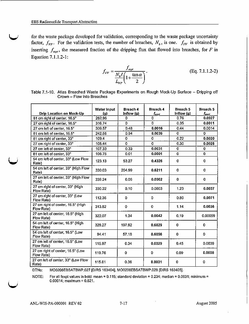
The experimentally measured fraction of the drip flux that flowed into all breaches (fp,) from
off-crown drip locations is given in Table 7.1-10. The breaches that were the focus of aparticular test or into which flow was expected have LIP, values shown in bold. For LIP, values
in bold, fexp, had a mean of 0.12, with a standard deviation of 0.23. The measured minimum
fraction was 0.0 and the maximum was 0.621.
Following the approach used in Section 6.5.1.1.3, the "inner cluster" splash diameter is used forthe effective length of the waste package in the validation of the flux splitting algorithm, whichis given by Equations 6.3.3.2-1 (or 6.5.1.1.3-2) and 6.3.3.2-3 (or 6.5.1.1.3-1). The form of theequation is:
F Nbe (ltan a'+= L2 t- "t fV, (Eq. 7.1.1.2-1)
where F is the fraction of dripping flux that flows through breaches, f is one-half the width of abreach or patch, L,,p is the effective length of the waste package (i.e., the length over which
dripping or splattering occurs), a is the rivulet spread angle, and fv,, is the uncertainty factor
ANL-WIS-PA-000001 REV 02 7-16 August 2005
EBS Radionuclide Transport Abstraction
for the waste package developed for validation, corresponding to the waste package uncertaintyfactor, f~jp. For the validation tests, the number of breaches, Nb, is one. fo, is obtained by
inserting fp,,, the measured fraction of the dripping flux that flowed into breaches, for F in
Equation 7.1.1.2-1:
Nbe1 tan1 a_L, 2
(Eq. 7.1.1.2-2)
Table 7.1-10. Atlas Breached Waste PackageCrown - Flow into Breaches
Experiments on Rough Mock-Up Surface - Dripping off
Water Input Breach 4 Breach 4 Breach 5 Breach 5Drip Location on Mock-Up (g) Inflow (g) feipt Inflow (g) fe, t
81 cm right of center, 16.50 282.96 0 0 0.76 0.0027
27 cm right of center, 16.50 316.74 0 0 0.35 0.0011
27 cm left of center, 16.50 309.57 0.48 0.0016 0.44 0.0014
81 cm left of center, 16.50 242.56 0.94 0.0039 0 0
81 cm right of center, 330 109.4 0 0 0.22 0.002027 cm right of center, 330 108.44 0 0 0.30 0.0028
27 cm left of center, 330 107.33 0.33 0.0031 0 081 cm left of center, 330 106.75 0.01 0.0001 0 0
54 cm left of center, 33* (Low Flow 123.13 53.27 0.4326 0 0Rate)54 cm left of center, 330 (High Flow 330.03 204.99 0.6211 0 0Rate)
27 cm left of center, 330 (High Flow 339.24 0.06 0.0002 0 0Rate)27 cm right of center, 33* (High 330.22 0.10 0.0003 1.23 0.0037Flow Rate)
27 cm right of center, 330 (Low 112.36 0 0 0.80 0.0071Flow Rate)27 cm right of center, 16.50 (High 313.82 0 0 1.14 0.0036Flow Rate)27 cm left of center, 16.50 (High 322.07 1.34 0.0042 0.19 0.00059Flow Rate)
54 cm left of center, 16.50 (High 328.27 197.92 0.6029 0 0Flow Rate)
54 cm left of center, 16.50 (Low 94.41 57.18 0.6056 0 0Flow Rate)
27 cm left of center, 16.50 (Low 115.97 0.34 0.0029 0.45 0.0039Flow Rate)27 cm right of center, 16.50 (Low 119.76 0 0 0.09 0.0008Flow Rate)
27 cm left of center, 330 (Low Flow 115.81 0.36 0.0031 0Rate) I I I _ 1 _ _ _
DTNs:
NOTE:
MO0208EBSATBWP.027 [DIRS 163404], MO0208EBSATBWP.028 [DIRS 163405].
For all fexpt values in bold: mean = 0.115; standard deviation = 0.234; median = 0.0031; minimum =0.00014; maximum = 0.621.
ANL-WIS-PA-000001 REV 02 7-17 August 2005

EBS Radionuclide Transport Abstraction
Statistics for f, are compared in Table 7.1-11 between the smooth surface experimental results
used for the waste package flux splitting submodel (Appendix D) and the rough surface resultsdiscussed in this section (Table 7.1-10).
Table 7.1-11. Comparison of fexpt Statistics for Smooth and Rough Surfaces
ExperimentsWaste Package (Smooth Surface)WP Validation (Rough Surface)WP = waste package
Mean fexpt
0.2950.115
Minimum fe&t Maximum f.,,t0.0 1.0660.0001 0.621
Median fe,,t
0.01420.0031
With the values for the breach flow fraction (fp,), the effective waste package length (L,,p),
and the spread angle (a) as determined above using off-crown rough surface test data, the rangefor fr,' is be determined. The half-width of the patch used in the experiments (t= 13.5 cm) is
used to evaluate fV,,. The minimum for fv,, is obtained using the minimum effective waste
package length (L,,p =6.0 cm) and the maximum spread angle (a = 19.00), resulting in
fv = 0. 3 7 9f, P,. The maximum for fi. is obtained using the maximum effective waste
package length (L,=30cm) and the minimum spread angle (a =00), resulting in
fn, = 2.22f4pg. Using the mean value of fv,, (0.115), fr, for the waste package ranges
from 0.044 to 0.26. Over the measured range of f.,p, (0 to 0.62 1), fv, ranges from 0.0
to (2.22)(0.621) = 1.38. The range obtained for f,,p (0.909 to 2.00), based on the mean smooth
surface value of f•,,, (0.295), is higher. When the measured range of smooth surface LIP,
values (0.0 to 1.066; see Figure D-10) for the waste package flux splitting analysis is usedinstead of the mean, f,,p ranges from 0.0 to 3.28. The waste package flux splitting submodel
(based on smooth surface data) overestimates flow through breaches compared to the modelvalidation estimates (based on rough surface data), which in turn overestimates the advectivereleases of radionuclides compared to the model validation estimates. The estimated values forfLP and fn, are summarized in Table 7.1-12.
Table 7.1-12. Summary of fwp and fvw Values
Based on Mean &ept Based on Minimum fept Based on Maximum fexpt
Minimum Maximum Minimum Maximumfwp 0.909 2.001 0.0 3.28fvw 0.044 0.26 0.0 1.38
ANL-WIS-PA-000001 REV 02 7-18 August 2005

EBS Radionuclide Transport Abstraction
As with the drip shield flux splitting submodel, a final comparison is between f,.,p, which lumps
the uncertainty in the rivulet spread angle into f;,p, and a corresponding parameter for the rough
waste package surface, f•,, where
f, = 1 + tana)fv,. (Eq. 7.1.1.2-3)
For the rough surface, a ranges from 00 to 19.0'. Applying the maximum value for a results inthe range for f~v of 0 to 0.30, based on the mean value of fexp,. For comparison, f1 was
estimated to range from 0 to 2.41. The wider range for f,' means that the waste package flux
splitting submodel tends to overestimate the flow through breaches in the waste packagecompared to the rough surface validation tests. The overlapping ranges for f".p and f~vvalidate the waste package flux splitting submodel.
Sections 7.1.1.1 and 7.1.1.2 have demonstrated that the drip shield and waste package fluxsplitting submodels based on experiments using smooth drip shield mock-up surfacesoverestimate fluxes when compared to the experimental data using rough drip shield mock-upsurfaces. The validations discussed uncertainties in relevant parameters. Based on thesevalidation results, the EBS flow model is adequate for its intended use.
7.1.2 Results of Independent Model Validation Technical Review of the EBS Flow Model
The results of the independent model validation technical review of the EBS flow model aregiven in a memo presented in Section 7.2.3 that combines the technical reviews of the EBS flowand transport models.
7.2 EBS TRANSPORT MODEL
The transport of radionuclides through the EBS is modeled, using assumptions in Section 5, as acombination of advective and diffusive transport including retardation between a series ofthree domains:
" Waste form domain* Corrosion products domain" Invert domain.
Advective transport is considered when water enters the waste form domain and is able to flowthrough the EBS and enter the UZ. The EBS flow model (Section 7.1) calculates the water fluxbetween each domain and a separate model provides radionuclide concentrations.
Diffusive transport between each of the domains occurs regardless of whether water is flowingthough the EBS, since, by Assumption 5.5, a continuous film of water is always present on allsurfaces of internal waste package components and corrosion products in a breached wastepackage when the temperature is below 100°C. Diffusive transport between each domain is
ANL-WIS-PA-000001 REV 02 7-19 August 2005

EBS Radionuclide Transport Abstraction
modeled in one dimension and therefore is dependent upon the following parameters that canvary as a function of time and according to the specific transport pathway:
* Effective diffusion coefficient* Diffusive area* Diffusion length.
The effective diffusion coefficient is calculated from Archie's law and is dependent upon the freewater diffusion coefficient, porosity, and saturation in each domain. Additionally a temperaturecorrection is made for diffusion in the invert domain. Porosity is either assumed to be constantor is provided by a separate model (e.g., BSC 2005 [DIRS 172895]). Saturation varies withrelative humidity. The diffusive area is calculated differently for each domain, but is either afunction of the number of breaches in the waste package (corrosion patches or stress corrosioncracks) or it is calculated from the geometry of the different components of the EBS. Thediffusive area of breaches also depends on the scenario class being modeled. The diffusionlength is either calculated from EBS geometry or is sampled, depending upon the domain.
As stated in Section 7, the level of confidence required for the EBS transport model is Level II.Level II validation is described in Section 7. In Sections 6.3 and 6.5, a detailed explanation andjustification is presented on the formulation of the transport model. These sections include agreat amount of information that is relevant to Level II validation. In addition, the followingsections include auxiliary information aimed to validate further certain components of thetransport model.
Section 7.2.1 describes a comparison between the in-package diffusion submodel and twosimilar, independently developed models of transport from a waste package to the invert. Thecomparison shows that although each model uses a different set of assumptions, the assumptionsused and the final diffusion coefficients calculated by each model generally agree and thus thetransport model is valid for its intended purpose.
Section 7.2.2 compares the invert diffusion coefficient of free water diffusivity for radionuclidesat different temperatures and with other cations and anions and shows that the self-diffusioncoefficient of water at 25°C is an upper bound.
7.2.1 In-Package Diffusion Submodel
Diffusive transport within the waste package will limit the release of radionuclides for thosewaste packages in a no-seep environment. The in-package diffusion submodel is directly relatedto the waste isolation attribute, limited release of radionuclides from the engineered barriers,because the model predicts delays in the release of mass from the waste package in comparisonto the TSPA-SR model, which immediately mobilized radionuclides at the external surface of thewaste package.
Level II validation is appropriate for the in-package diffusion submodel, as it is part of the EBSradionuclide transport model (see Section 7 above). In addition, the in-package diffusionsubmodel has the following features:
ANL-WIS-PA-000001 REV 02 7-20 August 2005

EBS Radionuclide Transport Abstraction
" The in-package diffusion submodel is not extrapolated over large distances or spaces.There is an inherent time extrapolation in the model.
" The in-package diffusion submodel bounds the uncertainties by consideringtwo bounding states. In the first state, the waste package internal components areconsidered to be in their intact, as-emplaced condition. For the second state, theiron-based waste package internal components are considered to be completely degradedto a porous material. Although these are two bounding end states, uncertainties exist inthe time- and spatially-dependent intermediate conditions.
" The in-package diffusion submodel has a minor impact on dose time history in the first10,000 years, based on sensitivity calculations performed for the prioritization reportRisk Information to Support Prioritization of Performance Assessment Models(BSC 2003 [DIRS 168796], Sections 3.3.6 through 3.3.11). Those studies indicate thatthe estimate of mean annual dose in the first 10,000 years has only a minor dependenceon in-package conditions that impact diffusion.
The in-package diffusion submodel is validated by comparison to two other models:
* Electric Power Research Institute (EPRI) Phase 5 report (EPRI 2000 [DIRS 154149])
* A model by Lee et al. (1996 [DIRS 100913]) for diffusive releases from waste packagecontainers with multiple perforations.
The in-package diffusion submodel is based on the one-dimensional diffusion equation, Fick'sfirst law of diffusion (Bird et al. 1960 [DIRS 103524], p. 503):
1L = -D ý-C . (Eq. 7.2.1-1)A ax
That is, the fundamental process being modeled is diffusion through a porous medium, a processthat is well understood and fully accepted throughout the scientific and engineering community.
Certain underlying assumptions need to be addressed. It is assumed that the bulk of thecorrosion products inside a waste package is hematite, Fe20 3, based simply on the predominanceof iron in the composition of internal non-waste form components. This assumption is also usedin the EPRI report (EPRI 2000 [DIRS 154149], p. 6-22), based on cited studies (EPRI 2000[DIRS 154149], p. 6-31) of corrosion products of carbon steel in humid, oxidizing environmentsthat indicate that in the presence of an abundant supply of oxygen, iron would be expected toexist as Fe 20 3, or FeOOH or Fe(OH) 3.
The specific surface area of hematite has been measured by numerous investigators. The rangeof values obtained varies widely, depending on the morphology of the sample. As can be seen inthe expressions for effective saturation and diffusion coefficient, Equations 6.3.4.3.5-5and 6.3.4.3.5-6, the diffusion coefficient is proportional to the square of the specific surface area,which from Table 6.3-7 varies by about a factor of about 12. This uncertainty is accounted for inthe uncertain parameter, SurfaceAreaCP (Table 6.5-6), which ranges from 1.0 to 22 m2 g-'
ANL-WIS-PA-000001 REV 02 7-21 August 2005

EBS Radionuclide Transport Abstraction
The water adsorption isotherm used for the in-package diffusion submodel is compared withanother measured isotherm (McCafferty and Zettlemoyer 1971 [DIRS 154378], Figure 3) inFigure 7.2-1, which shows the close agreement between independent investigators. In addition,Figure 6.3-6 shows that hematite over-predicts the amount of water adsorbed compared to nickeloxide, which is one of the other major components of stainless steel(DTN: M00003RIB00076.000 [DIRS 153044]) that would comprise the products of corrosionof the waste package internal components.
Adsorption IsothermWater on a-Fe 203
10
9
8
'-7
•_ 6r -- e--Jurinak
"5•_ - - -•-McCafferty &40 Zettlemoyer
E
Z 3
2
1E
0 0.2 0.4 0.6 0.8RH
154 0402,ai
Source: Jurinak curve: Jurinak 1964 [DIRS 154381]; McCafferty and Zettlemoyer curve: McCafferty andZettlemoyer 1971 [DI RS 154378].
Figure 7.2-1. Adsorption Isotherms for Water Vapor on a- Fe203
7.2.1.1 Comparison with Electric Power Research Institute 2000
Validation of the in-package diffusion submodel is provided in part by qualitative comparisonwith a similar model developed independently by a reputable performance assessment program(EPRI 2000 [D1RS 154149]).
The EPRI source-term model, COMPASS2000, implements five compartments-Waste,Corrosion Products, Canister, Invert, Near-Field Rock-of which two (Corrosion Products andCanister) are analogous to portions of the in-package diffusion submodel. The Corrosion
ANL-WIS-PA-000001 REV 02 7-22 August 2005
EBS Radionuclide Transport Abstraction
Products compartment represents the porous material that is formed after the basket materials arecorroded. The Canister compartment represents the failed metal canisters. As with the GoldSimTSPA-LA model, each compartment is treated as a mixing cell in which radionuclideconcentrations are assumed to be uniform. Mass balances in each compartment account for thevarious processes that comprise the model, including transport by diffusion and advection,radioactive decay and ingrowth, sorption, dissolution, and precipitation.
In the EPRI model, EBS transport parameters are assigned fixed values. Both the CorrosionProducts and corroded Canister compartments have a porosity of 0.42 (EPRI 2000[DIRS 154149], p. 6-21), less than the initial porosity of a CSNF waste package, 0.58, asestimated in Section 6.3.4.3.4. The EPRI value accounts for the volume occupied by the oxide.A lower value for porosity overestimates releases of radionuclides. However, in the in-packagediffusion submodel (Equation 6.3.4.3.5-6), the higher value of porosity increases the estimateddiffusion coefficient by only a factor of 1.5, which is small compared to other uncertainties inthe model.
The EPRI model assumes a fixed water saturation of 0.35 in both the Corrosion Products andcorroded Canister compartments (EPRI 2000 [DIRS 154149], p. 6-21). This value is appropriatefor modeling cases involving advective transport, but overestimates releases of radionuclides forthe expected large fraction of the repository that has no seepage flux, where the only waterpresent is adsorbed water. The in-package diffusion submodel specifically applies to thoseregions and provides a more realistic estimate of saturation as a function of relative humidity.
The EPRI model uses a fixed value for effective diffusion coefficient of 4.645x10⁻⁴ m2 yr- inboth the Corrosion Products and corroded Canister compartments (EPRI 2000 [DIRS 154149],p. 6-22). This converts to 1.472 x 10⁻⁷ cm2 S-1 or to 1.472 x 10⁻¹¹ m2 s-1. For diffusion througha fully degraded waste package (Equation 6.3.4.3.5-5), this corresponds to a relative humidityof 97.9 percent. Thus, when the humidity is high, the EPRI model and the in-package diffusionsubmodel agree well. In contrast, the in-package diffusion submodel provideshumidity-dependent diffusion coefficient values.
The EPRI model also specifies fixed diffusive lengths, which are defined as the distance from thecenter of the compartment to the interface of the two contacting compartments. For theCorrosion Products compartment, the diffusion length is 0.046 m; for the Canister compartment,the diffusion length is 0.025 m (EPRI 2000 [DIRS 154149], p. 6-22). In a well-degraded wastepackage, these are reasonable values, comparable to those used in the in-package diffusionsubmodel. However, the in-package diffusion submodel accounts for the uncertainty in diffusionlengths at all times, and provides special treatment at early times when large masses of corrosionproducts are not yet formed.
For the conditions assumed in the EPRI model, namely, at later times when the waste package isextensively corroded, the in-package diffusion submodel agrees quite well with the EPRI model.The primary differences are that the in-package diffusion submodel accounts for a wider range ofconditions, including times just after breaches first appear in the waste package. In addition, thein-package diffusion submodel accounts explicitly for the relative humidity, which realistically isthe only source of water when seepage does not occur. And finally, in contrast to the EPRImodel, the in-package diffusion submodel accounts for uncertainty in diffusive path lengths.
ANL-WIS-PA-000001 REV 02 7-23 August 2005

EBS Radionuclide Transport Abstraction
Thus, there is agreement between the models, and where differences occur, it is primarily toincrease the realism of the diffusive release calculation and to account for uncertainty.
7.2.1.2 Comparison with Lee et al. 1996
Validation of the in-package diffusion submodel is provided in part by comparison with a similarmodel developed independently and published in technical literature (Lee et al. 1996[DIRS 100913]).
Lee et al. (1996 [DIRS 100913]) developed a model for steady-state and "quasi-transient"diffusive releases from waste packages into the invert. In this model, perforations in the packageare assumed to be cylindrical in shape. The diffusion path consists of the approach to theopening of the perforation from the waste form side; the path through the cylindrical portion ofthe perforation, which is filled with corrosion products; and the path through the exit diskseparating the perforation from the invert. The waste is assumed to be distributed uniformlyinside the waste container. The package is approximated by an equivalent sphericalconfiguration, and the underlying invert is represented by a spherical shell surroundingthe package.
The model of Lee et al. (1996 [DIRS 100913]) is suitable for the late stages of packagedegradation, when the waste form has become a mass of porous corrosion products. AlthoughLee et al. (1996 [DIRS 100913]) assumed the packages failed by localized corrosion, this modelshould be equally applicable to failure by general corrosion.
The assumption of Lee et al. (1996 [DIRS 100913]) that the waste (i.e., the radionuclide source)is uniformly distributed inside the waste package restricts the applicability of the model andcomparison to the in-package diffusion submodel to the times when the waste package hasextensively corroded. The object of the in-package diffusion submodel is to provide morerealism at earlier and intermediate times, when the waste cannot yet be considered a uniformporous medium. (In the in-package diffusion submodel, the dependence of the diffusiveproperties of the waste package on the extent of degradation is computed explicitly as a functionof time; see Sections 6.3.4.3.5 and 6.5.3.2.) On the other hand, the fundamental assumption thatdiffusive releases are controlled by diffusion through breaches that are filled with porouscorrosion products may be valid over much of the waste package lifetime, including early times,when stress corrosion cracks are the first breaches to appear. Lee et al. (1996 [DIRS 100913],p. 5-67) assume that the porosity of the perforations is tcp = 0.4, and the volumetric watercontent is 0 =10 percent (so the water saturation in the perforations is a constantS., ='F/(I00qcp)= 0.25). Based on data by Conca and Wright (1990 [DIRS 101582]; 1992
[DIRS 100436]), Lee et al. compute a diffusion coefficient, D (cm. s-1), for the porous corrosionproducts filling the perforations (Lee et al. 1996 [DIRS 100913], p. 5-67):
log1 0 D = -8.255(±0.0499) +1.898(±0.0464) log1 0 1, (Eq. 7.2.1.2-1)
where the numbers in parentheses are one standard deviation. From the discussion inSection 6.3.4.1.1, it is likely that this equation, being based on data by Conca and Wright (1990[DIRS 101582]; 1992 [DIRS 100436]), should be written using loglo(qcpSD) rather than
ANL-WIS-PA-000001 REV 02 7-24 August 2005

EBS Radionuclide Transport Abstraction
logl0 D; however, this model validation comparison will use the equation as given by Lee et al.,since not enough information is available to repeat their analysis.
For (1 0 percent (the assumed volumetric water content of the perforations),Equation 7.2.1.2-1 gives D = 4.4 x 10⁻⁷ cm 2 s-1. Lee et al. assume that the diffusion coefficientinside the waste package (as opposed to the perforations) is 10-5 cm 2 s-1 (Lee et al. 1996[DIRS 100913], p. 5-67). As a comparison, the self-diffusion coefficient for wateris 2.299 x 10- 5 cm 2 s-' (Mills 1973 [DIRS 133392], Table III), and for many actinides thediffusion coefficient in water is roughly 5 x 10⁻⁶ cm 2 s-1 (Table 7.2-11). The value for Dobtained from Equation 7.2.1.2-1 (4.4 x 10- cm2 s-1) accounts for porosity, saturation, andtortuosity, and thus is comparable to the values forD, obtained from Equation 6.3.4.3.5-6.
Table 6.3-10 tabulates values of •zS,,D, using Equation 6.3.4.3.5-6. At appropriate ranges of
conditions in Table 6.3-10 for a water content of 10percent, D. ranges from
about 1.4 x 10⁻⁶ cm 2 s-1 to about 4.1 X 10⁻⁶ cm 2 S-1 (in Table 6.3-10, where, for the lower boundon specific surface area of 'cp = 1,000 m2 kg', the closest entry for 10 percent water content,
OS, is OSS,,D, = 1.4 x 10⁻⁷ cm 2 s-1, at RH = 0.9999, and S,,.e =0.14; for the upper bound on
specific surface area of 7cp = 22,000 m2 kg-1, at a water content of approximately 10 percent,
OS.,D, =4.1 x 10⁻⁷ cm 2 s-1, at RH = 0.95 and S,, =0.24). This comparison indicates that the
model developed by Lee et al. (1996 [DIRS 100913]) for D represents high relative humidity andreasonable specific surface area (i.e., within the sampled range specified for the EBS RTAbstraction) if adsorption is the sole mechanism for water appearing in the corrosion products.
A more detailed calculation can be performed to estimate the surface area of corrosion patches,the amount of water adsorbed at various relative humidity values, the resulting water saturationof the patches, and obtain a diffusion coefficient using Equation 6.3.4.3.5-6. Alternatively, thediffusion coefficient can be obtained using a modification of Equation 7.2.1.2-1, in which thewater content, 0 (percent), is:
= lOOS,,.,cpqcp = 1.194(- In RH)-)° 40°. (Eq. 7.2.1.2-2)
This equation uses a porosity of Ocp = 0.4, but obtains the effective water saturation fromEquation 6.3.4.3.5-5, which is based on the assumption that all water comes from adsorption ofwater vapor onto hematite having a specific surface area of 9.1 m2 g-1. Then, substitutingEquation 7.2.1.2-2 into Equation 7.2.1.2-1:
logl0 D = -8.255 + 1.898log1 0 (D
= -8.255 + 1.898[0.07707 - 0.408 log10 (- In RH)] (Eq. 7.2.1.2-3)
= -8.109- 0.7751ogl 0(- InRH).
For example, at RH = 0.95, the effective diffusion coefficient for the patch usingArchie's law (Equation 6.3.4.3.5-6) is OS,,D, = 7.03 x 10⁻¹² m2 s-1 (for 0b = 0.4 and,
ANL-WIS-PA-000001 REV 02 7-25 August 2005

EBS Radionuclide Transport Abstraction
from Equation 6.3.4.3.5-5, S.,=0.100), or D,=1.75x 010- m2 s-, whereas using
Equation 7.2.1.2-3, the diffusion coefficient for the corrosion patch is D = 7.77 x 10⁻¹ M2 s-1 .
Thus, for those cases where the release rate is controlled by diffusion through porous corrosionproducts, the in-package diffusion submodel results in more rapid diffusive releases than themodel of Lee et al. (1996 [DIRS 100913]).
If the value obtained by Lee et al. is actually log10 (OcpSD) rather than logl0 D, then the two
models agree well. For example, at a water content S,,Sw = D of 10 percent, Equation 7.2.1.2-1
would give ,AS,'D =4.4 x 10⁻⁷ cm 2 s-1 or D =4.4 x 104 cm 2 s- 1, which compares well with the
range of D, from Table 6.3-10 of 1.4 x 10⁻⁶ cm2 s-1 to 4.1 X 10⁻⁶ cm 2 s") at a water content of
approximately 10 percent, as discussed earlier in this section.
The in-package diffusion submodel provides a means for quantifying the uncertainty in diffusioncoefficients for diffusion of radionuclides from within the waste form to the invert. Whereasother models consider only the times when the waste package is largely degraded, the in-packagediffusion submodel presented here also considers earlier times, starting from the time of theinitial waste package breach. The time period between initial breach and complete degradationof the internal components may span many thousands of years. Thus, the in-package diffusionsubmodel fills a major time gap in modeling diffusive releases from a waste package. In effect,it provides a rationale for interpolating between essentially a zero diffusion coefficient (due tothe absence of water) when a waste package is first breached to a value at a time when porouscorrosion products can be expected to fill the waste package with a degree of water saturationcapable of transporting radionuclides. The in-package diffusion submodel is consideredvalidated based on corroborating data for input parameters such as water adsorption isothermsand specific surface areas, and based on the agreement with two other waste package diffusionmodels in areas where these models apply.
7.2.2 Invert Diffusion Submodel
Level I validation is appropriate for the invert diffusion submodel, as it is part of the mechanismsfor radionuclide transport from waste package to the drift wall through the invert (see Section 7).In addition, the invert diffusion submodel has the following features:
Diffusive release from the engineered barrier system does not result in significantreleases from the repository system. Under expected conditions, there is a smallprobability of waste package breaching, and only limited release at all is likely.Therefore, the diffusion properties of the invert that might affect this release are expectedto play a small role in the estimate of performance of the system under these conditions.The invert diffusion coefficient is also expected to play a small role for disruptiveconditions under which more significant breaching of the waste package might occur. Inthis case, transport through the invert would be dominated by advection, and diffusionwould therefore provide only a minor contribution. Therefore, the diffusion submodel isnot expected to play a major role in the assessment of system performance.
ANL-WIS-PA-000001 REV 02 7-26 August 2005

EBS Radionuclide Transport Abstraction
In addition to the above, the invert diffusion properties submodel is not extrapolatedbeyond the conditions and distances considered in the development of the model. Themodel applies only on the scale of the EBS and is not applied to larger scales, forexample to the unsaturated zone rock.
The invert diffusion coefficient abstraction considers the free water diffusivity for radionuclidesas an upper bound. The validation of each of these factors is considered in thefollowing sections.
Section 6.3.4.1.2 describes modification of the self-diffusion coefficient due to temperature. Themodification is based on established principles of diffusion in fluids and thus no validation isnecessary. The temperature modification is based on the relationship between diffusion andviscosity and temperature (Cussler 1997 [DIRS 111468], p. 114). The relationship betweentemperature and viscosity of water is available in text books. Thus, it is straightforward toestablish a direct relationship between diffusion coefficient and temperature.
7.2.2.1 Self-Diffusion Coefficient of Water
The self-diffusion coefficient of water at 25°C, 2.299 x 10⁻⁵ cm 2 s-1 (Mills 1973 [DIRS 133392],Table III), provides an upper bound for the diffusion of ionic and neutral inorganic, andorgano-metal species that may be released from a waste package. This assertion is based on thefollowing points, which are discussed in the text following this list:
1. A survey of compiled diffusion coefficients at 25'C shows that simple cation andanion species (excluding the proton and hydroxyl species, which are not appropriateanalogs to diffusing radionuclide species) have diffusion coefficients that are smallerthan that of water.
2. The self-diffusion coefficient for water at 90'C is larger than compiled diffusioncoefficients for simple inorganic species at 100IC.
3. Diffusion coefficients for simple lanthanide and actinide cations are much smaller thanthe self-diffusion coefficient of water and are expected to be even smaller for theirhydroxyl and carbonate complexes.
In a compilation of diffusion coefficients for 97 ionic species , only 3 species, H÷, OH-, and 0D-have diffusion coefficients at 25'C that are larger than the self-diffusion of water at 25'C (Millsand Lobo 1989 [DIRS 138725], Appendix A, Tables 1.1 to 1.6, pages 314 to 319). Ofthe 33 ionic species for which Mills and Lobo list diffusion coefficients at 100°C in Tables 1.1through Table 1.7, only 2 species, H÷ and OH-, have diffusion coefficients larger than theself-diffusion of water (H2
180) at 90 0C (Mills and Lobo 1989 [DIRS 138725]; Table 1, page 17).The fact that the self-diffusion of H2
180 is less than that of H20, and that the self-diffusion ofH20 at 90'C would be greater than that of various ionic species at 100'C, further supports thecontention that the self-diffusion of water at 25'C is bounding.
ANL-WIS-PA-000001 REV 02 7-27 August 2005

EBS Radionuclide Transport Abstraction
Using the self-diffusion coefficient for water as a bounding value for all radionuclides partiallycompensates for not accounting for the effect of temperature on the diffusion coefficient in thecorrosion product domain. See the discussion at the end of Section 6.3.4.3.5.
The compilation below (Table 7.2-1) lists a selection of diffusion coefficients for some trivalentlanthanides and actinides. Table 7.2-1 also includes some anions not listed in most compilationsbut relevant and/or analogous to those expected for radionuclides released from the wastepackage. The listing shows that the diffusion coefficients for these species are all smaller thanthe self-diffusion of water, by factors ranging from 1.6 to 14.7. In the case of uranium, thecarbonate complexes of the metal species have even smaller diffusion coefficients. Based on theStokes-Einstein equation (Bird et al. 1960 [DIRS 103524], p. 514, Equation 16.5-4), thediffusivity of a solute in a liquid is inversely proportional to the radius of the diffusing particles.It is therefore expected that other carbonate and hydroxyl complexes, on the basis of the greatersize of the complexes relative to the metal species, will also have smaller diffusion coefficientsthan the metal species listed in Table 7.2-1.
As an alternative, four diffusion coefficients could be used. One coefficient could be used foreach charge (mono-, di-, and tri-valent species) and one for the hydroxyl and carbonatecomplexes of the actinides and lanthanides. At 25'C, the mono-, di-, and trivalent species havebounding values of 2.2 x 10⁻⁵ cm 2 s-1, 1.2 x 10⁻⁵ cm 2 s-1 , 0.7 x 10⁻⁵ cm 2 s-1, respectively, asshown in Figure 7.2-2. Although this alternative model is not used for TSPA-LA, it providesfurther evidence that the use of the self-diffusion coefficient of water bounds the diffusioncoefficients of diffusing radionuclide species in the EBS.
ANL-WIS-PA-000001 REV 02 7-28 August 2005
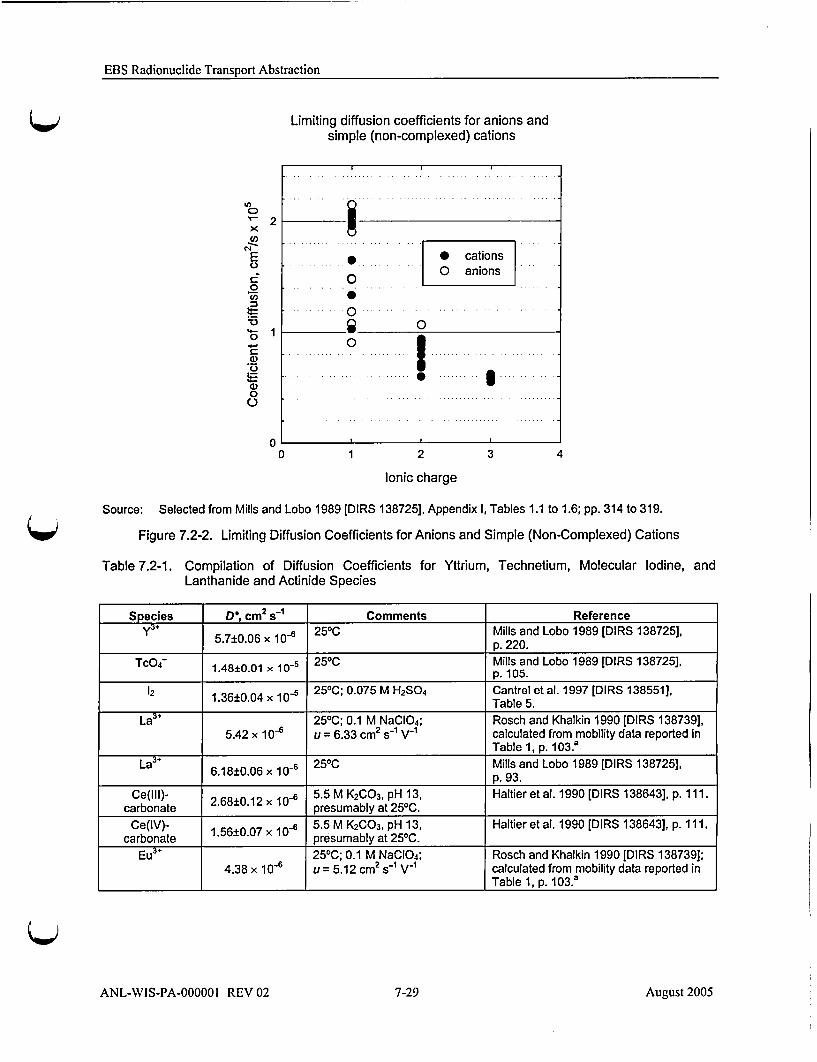
EBS Radionuclide Transport Abstraction
In
E
t.2
C-)C0
0
0
2
1
0
Limiting diffusion coefficients for anions andsimple (non-complexed) cations
0 cations0 anions
0
0.. .. .O ... . . . ... . . . . . . . . . . . .
.. 0
I ~I
0 1 2 3 4
Ionic charge
Source: Selected from Mills and Lobo 1989 [DIRS 138725], Appendix I, Tables 1.1 to 1.6; pp. 314 to 319.
Figure 7.2-2. Limiting Diffusion Coefficients for Anions and Simple (Non-Complexed) Cations
Table 7.2-1. Compilation of Diffusion Coefficients for Yttrium, Technetium, Molecular Iodine, andLanthanide and Actinide Species
Species D*, cm2 s-1 Comments Referencey3. 5.7±0.06 x 10⁻⁶ 25 0C Mills and Lobo 1989 [DIRS 138725],
p. 220.Tc04- 1.48±0.01 x 10-s 250C Mills and Lobo 1989 [DIRS 138725],
p. 105.12 1.36±0.04 x 10⁻⁵ 250 C; 0.075 M H2SO 4 Cantrel et al. 1997 [DIRS 138551],
Table 5.La3
+ 25°C; 0.1 M NaCIO 4; Rosch and Khalkin 1990 [DIRS 138739],5.42 x 10-' u = 6.33 cm2 s-1 V-1 calculated from mobility data reported in
Table 1, p. 103.aLa3' 6.18±0.06 x 10⁻⁶ 25°C Mills and Lobo 1989 [DIRS 138725],
p. 93.Ce(lll)- 2.68±0.12 x 10⁻⁶ 5.5 M K2CO 3, pH 13, Haltier et al. 1990 [DIRS 138643], p. 111.
carbonate presumably at 250C.Ce(IV)- 1.560.07 x 10-6 5.5 M K2C0 3, pH 13, Haltier et al. 1990 [DIRS 138643], p. 1 1 1.
carbonate presumably at 250C.Eu 3 25 0C; 0.1 M NaCIO 4; Rosch and Khalkin 1990 [DIRS 138739];
4.38 x 10' u = 5.12 cm2 s-1 V-1 calculated from mobility data reported inI Table 1, p. 103.a
ANL-WIS-PA-000001 REV 02 7-29 August 2005

EBS Radionuclide Transport Abstraction
Table 7.2-1. Compilation of Diffusion Coefficients for Yttrium, Technetium, Molecular Iodine, andLanthanide and Actinide Species (Continued)
Species D* cm2 s-1 Comments ReferenceGd'÷ 250C; 0.1 M NaCIO 4; Rosch and Khalkin 1990 [DIRS 138739];
5.24 x 10⁻⁶ u = 6.12 cm2 s-1 V- 1 calculated from mobility data reported inTable 1, p. 103.'
Tb3÷ 250C; 0.1 M NaCIO 4; Rosch and Khalkin 1990 [DIRS 138739];5.01 x 10⁴ u = 5.85 cm2 s-1 V-1 calculated from mobility data reported in
Table 1, p. 103.8Tm3÷ 250C; 0.1 M NaClO 4; Rosch and Khalkin 1990 [DIRS 138739],
5.10 x 10⁻⁶ u = 5.96 cm2 s- 1 V-1 calculated from mobility data reported inTable 1; p. 103.'
Yb 3÷ 250C; 0.1 M NaCIO 4; Rosch and Khalkin 1990 [DIRS 138739],5.23 x 10-6 u = 6.11 cm 2 s-1 V-1 calculated from mobility data reported in
Table 1; p. 103.'Lu3÷ 250C; 0.1 M NaCIO 4; Rosch and Khalkin 1990 [DIRS 138739],
5.01 x 10⁻⁶ u = 5.85 cm 2 s-1 V-1 calculated from mobility data reported inTable 1; p. 103.'
UO 2(CO 3)34- 3.6 x 10- 1 M total carbonate, 220C Perry et al. 1988 [DIRS 138732], p. 302.U0 2(CO 3)3'L 3.0±0.7 x 10⁻⁶ 0.2 M total carbonate, pH 9.8, Perry et al. 1988 [DIRS 138732], p. 302.
250CUO 2(CO 3)3 - 3.81±0.26 x 10⁻⁶ 0.75 M Na2CO 3, 0.6 M NaClO 4, Haltier et al. 1990 [DIRS 138643], p. 110.
pH 11.5, presumably at 25 0CU02+* 6.8 x 10⁻⁶ 250C Millard and Hedges 1996 [DIRS 138677],
p. 2141.U02-carbonate Calculated using Stokes- Millard and Hedges 1996 [DIRS 138677],
1.9 x 10⁻⁶ Einstein with a radius of p. 2141.8 A at 100C
Np(V)-carbonate Calculated using Stokes- Tsukamoto et al. 1994 [DIRS 138747]; p.7 x 10-6 Einstein with a radius of 469.
3.4 A at 250CAm3÷ 250C; 0.1 M NaCIO4; Rosch and Khalkin 1990 [DIRS 138739];
5.78 x 10⁻⁶ u = 6.75 cm2 s-1 V"1 calculated from mobility data reported inTable 1; p. 103.a
Am3÷ 5.95±0.06 x 10⁻⁶ 250C, in 0.0002 M Nd(CI0 4)3 Mills and Lobo 1989 [DIRS 138725];p. 131.
CO+ 250C; 0.1 M NaClO 4; Rosch and Khalkin 1990 [DIRS 138739];4.39 x 10⁻⁶ u = 5.13 cm 2 s-1 V-1 calculated from mobility data reported in
Table 1; p. 103.aCf3O 5.50±0.06 x 10⁻⁶ 250C, in 0.0002 M Nd(CI0 4)3 Mills and Lobo 1989 [DIRS 138725];
p. 132.
Es 3÷ 5.50±0.06 x 10⁻⁶ 250C, in 0.0002 M Nd(CI0 4)3 Mills and Lobo 1989 [DIRS 138725];p. 132.
a Calculation of diffusion coefficients from reported ionic mobilities (Rosch and Khalkin 1990 [DIRS 138739];Table 1). The mobilities (u) were measured in 0.1 M NaCIO4 at various pHs (below the pH of hydrolysis) andwere slightly larger at pHs greater than 5, and these are the data that were used for the calculation. The equationused to calculate the diffusion coefficient is: D* = (kT/(Izje)) u, where k is Boltzmann constant (J K-1), Tis thetemperature (K), z is the valence of the ion, e is the elementary charge (C), and u is the mobility (cm2 s- V- )(Atkins 1990 [DIRS 111464], Box 25.1, Einstein relation, p. 765).
ANL-WIS-PA-000001 REV 02 7-30 August 2005

EBS Radionuclide Transport Abstraction
7.2.2.2 Modification for Porosity and Saturation
Validation of the dependence of invert diffusion coefficient on porosity and saturation isprovided by comparison with measured data obtained independently of the data used for modeldevelopment. Data used for validation are obtained from diffusivity measurements for crushedtuff using electrical conductivity measurements (CRWMS M&O 2000 [DIRS 156680]) and fromdirect measurements of diffusivity between machined cubes of tuff (Hu et al. 2001[DIRS 161623]).
Conca and Wright (1992 [DIRS 100436]) and Conca et al. (1993 [DIRS 170709]) obtaineddiffusion coefficients from electrical conductivity measurements for various granular materials,including tuff, with volumetric moisture content ranging from 0.5 percent to 66.3 percent. Astatistical fit of the data (Conca and Wright 1992 [DIRS 100436], Figure 2; Conca et al. 1993[DIRS 170709], Figure 2; listed in Table 4.1-17) ranging from 1.5 percent to 66.3 percentvolumetric moisture content, based on Archie's law, results in the model used in TSPA-LA(Section 6.3.4.1.1 and Appendix G):
OD, = D0qi.' 8 63 s I ': 8 63 10 ND(p=0.033,aT=0.218)
= Do _9 1.863 1 0 ND(i=o.o33.=o.218) (Eq. 7.2.2.2-1)
where 0 = OS,. is the volumetric moisture content (fraction: m3 water m-3 rock), and ND
represents a normal distribution with a mean, u, of 0.033 and a standard deviation, ar, of 0.218.The object of this validation is to show that the diffusion coefficient given by Equation 7.2.2.2-1obtained from the electrical conductivity measurements of Conca and Wright (1992 [DIRS100436]) and Conca et al. (1993 [DIRS 170709]) tends to overestimate the diffusivity ofinvert materials.
The diffusion coefficient has also been determined specifically for tuff, also using electricalconductivity measurements (CRWMS M&O 2000 [DIRS 156680], Tables A-1 and A-2). Thesedata are listed in Table 7.2-2 and are plotted in Figure 7.2-3, along with the mean value and plusand minus three standard deviations from Equation 7.2.2.2-1. This plot shows that the fit to themeasured diffusion coefficient data (Equation 7.2.2.2-1) overestimates the diffusion coefficientrelative to The Determination of Difiision Coefficient of Invert Materials (CRWMS M&O 2000[DIRS 156680], Tables A-1 and A-2). This plot was created using Microsoft Excel; seeAppendix G, Worksheet: Validation, p. VII-10.
The electrical conductivity measurements by Conca and Wright (1992 [DIRS 100436]) andConca et al. (1993 [DIRS 170709]) use conductivity as an analog for diffusivity. While theanalog is known to be valid in fully saturated media, its application to unsaturated media,particularly at low moisture contents, is questionable due to the difficulty in preparing samplesand in making reliable electrical contact between the electrical leads and the samples. To avoidthese problems, Hu et al. (2001 [DIRS 161623]) measured diffusive tracer concentrations in tuffcubes directly using laser ablation coupled with inductively coupled plasma-mass spectrometry(LA-ICP-MS), rather than relying on electrical analogs.
ANL-WIS-PA-000001 REV 02 7-31 August 2005
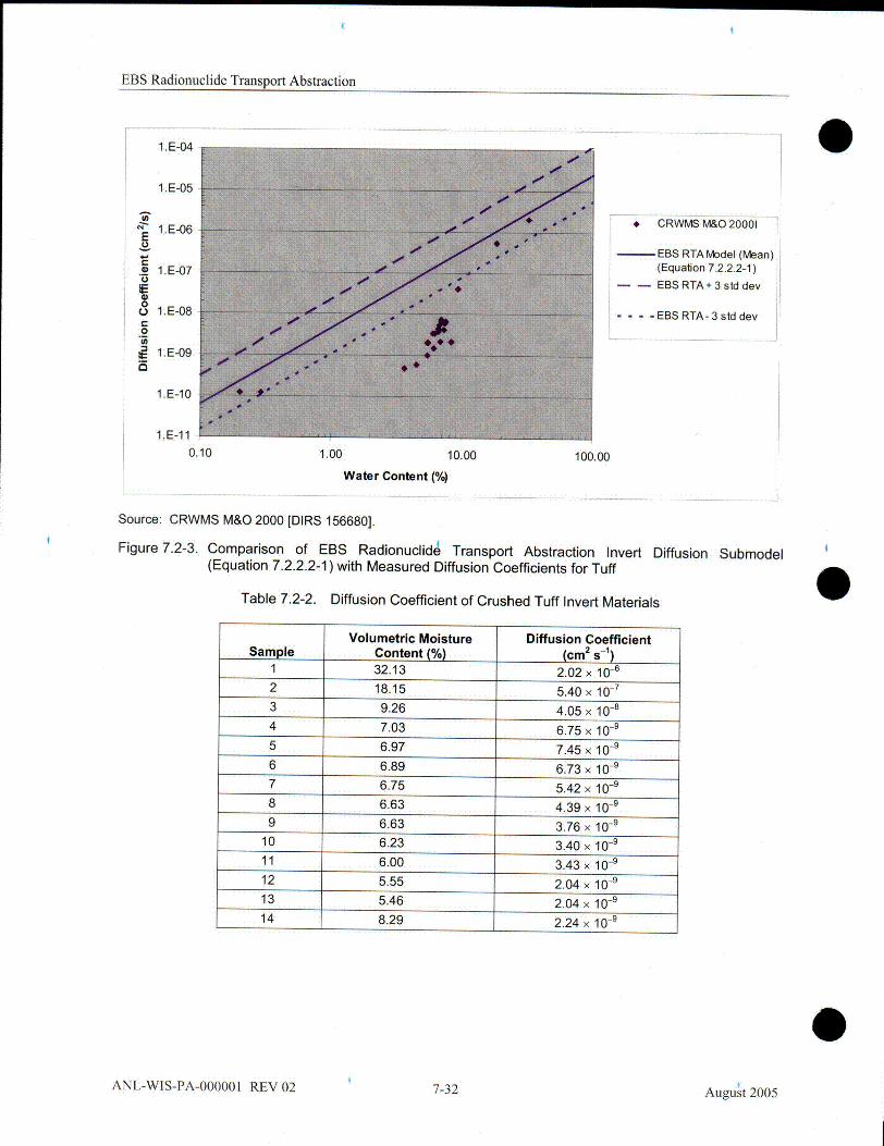
EBS Radionuclide Transport Abstraction
01.E-04
1.E-05
S1 .E-06E
S1.E-07
.2
* 1.E-090 1 .E-08
S1.E-09
1.E-10
1.E-110.10
* CRWMS M&O 20001
EEBS RTA Model (Mean)(Equation 7.2.2.2-1)
S-EBS RTA + 3 std dev
--- -EBS RTA- 3 stddev
1.00 10.00
Water Content (%)
100.00
Source: CRWMS M&O 2000 [DIRS 156680].
Figure 7.2-3. Comparison of EBS Radionuclide Transport Abstraction Invert Diffusion Submodel(Equation 7.2.2.2-1) with Measured Diffusion Coefficients for Tuff
Table 7.2-2. Diffusion Coefficient of Crushed Tuff Invert Materials
Volumetric Moisture Diffusion CoefficientSample Content (%) (cm2 s-1)
1 32.13 2.02 × 10-62 18.15 5.40 x 10⁻⁷
3 9.26 4.05 x 10⁻⁸
4 7.03 6.75 x 10'5 6.97 7.45 x 10⁻⁹
6 6.89 6.73 x 10-'7 6.75 5.42 x 10-'8 6.63 4.39 x 10-'9 6.63 3.76 x 10⁻⁹
10 6.23 3.40 x 10⁻⁹
11 6.00 3.43 x 10'12 5.55 2.04 x 10-'13 5.46 2.04 x 10-'14 8.29 2.24 x 10-
ANL-WIS-PA-000001 REV 02 7-32 August 2005

EBS Radionuclide Transport Abstraction
Table 7.2-2. Diffusion Coefficient of Crushed Tuff Invert Materials (Continued)
Volumetric Moisture Diffusion CoefficientSample Content (%) (cm2 s-1)
15 7.54 6.81 x 10⁻⁹
16 7.36 6.21 x 10⁻⁹
17 7.22 4.38 x 10-918 6.84 2.19 x 10-919 6.11 1.55 x 10⁻⁹
20 5.41 9.97 x 10-l
21 4.45 6.19 x 10-1022 3.64 5.00 x 10-1023 0.29 1.24 x 10⁻¹°
24 0.20 1.25 x 10⁻¹⁰
Source: CRWMS M&O 2000 [DIRS 156680], Tables A-1 and A-2.
LA-ICP-MS has recently evolved as a powerful analytical tool for solid samples (Russoet al. 2000 [DIRS 155697]). It can simultaneously determine a large number of chemicalelements with low detection limits. Laser ablation uses an intense burst of energy delivered by ashort laser pulse to vaporize a minute sample (in the range of nanograms) from a small area.Several spot sizes can be selected (from 25 /am to 200 /m in diameter), allowing a choice ofappropriate spot size for different applications. A smaller spot size will sample less solidmaterial, leading to lower analytical precision, but allowing more heterogeneity to be observed.A single laser pulse reveals surface compositions, while multiple pulses allows compositions tomeasured at various depths below the surface, with the crater depth proportional to the number oflaser pulses applied. For example, two pulses reach about 4 pm into the tuff matrix(Hu et al. 2001 [DIRS 161623], p. 22), and 50 pulses ablates to a depth of about 35 jm(Hu et al. 2001 [DIRS 161623], Figure 6).
In the approach of Hu et al. (2001 [DIRS 161623]), a machined 1.5-cm tuff cube containing atracer was placed in contact with a cube not containing the tracer, both under the samethermodynamic conditions. The tracer is allowed to diffuse from the tracer-containing cube tothe other. Tracers were chosen based on their chemical similarity to radionuclides of interest.The source cube was vacuum-saturated with a tracer solution mixture of NaBr, NaReO 4, CsBr,and RbBr; both BF and perrhenate (ReO4-) act as nonsorbing tracers. The sink cube was alsovacuum-saturated, but had no tracers. Source and sink cubes were separately placed inside ahumidity chamber within an incubator maintained at 22'C until the cubes equilibrated to aconstant weight (13 days). The cubes were then clamped together in the relative humidity (RH)chamber to start the diffusion test. After 87 days, the diffusion test was stopped by separatingthe source and sink cubes. The surface and depth distribution of the tracer was then mappedusing LA-ICP-MS. The mapping was done on the interface, the far side face (opposite side fromthe interface), and along the side perpendicular to the interface.
Measurements along the outside surface of the sink cube indicated that a nonsorbing tracer(ReO4") diffused along the surface at a rate similar to its aqueous diffusion rate in bulk water(Hu et al. 2001 [DIRS 161623], pp. 21 and 22). This result was reasonable because the tuffcubes were located in the high-RH chamber, with the likely presence on the outside of the cube
ANL-WIS-PA-000001 REV 02 7-33 August 2005

EBS Radionuclide Transport Abstraction
of a thick water film that behaves like bulk water. These measurements provided a boundingvalue for the diffusivity of the tracer, comparable to the diffusion coefficientof 1.48x10⁻⁵ cm 2 S-1 (Table 7.2-1) for its analog, Tc04-. In other words, in regions on the tuffsamples that were saturated or at least had high water saturation, the direct diffusivitymeasurements agreed with theoretical predictions.
Hu et al. also measured tracer concentrations at greater depths into the cube by using the laserablation technique to probe into the surface. They found that internal diffusion coefficients, atdepths of 60-410 ptm, were on the order of 10-12 cm 2 s- 1 (Hu et al. 2001 [DIRS 161623], p. 22).The measured volumetric water content of the tuff matrix was 8.9 percent (Hu et al. 2001[DIRS 161623], p. 25). The mean diffusion coefficient predicted by the invert diffusionproperties submodel (Equation 7.2.2.2-1) would then be 2.6 x 10⁻⁷ cm 2 s- 1. This is a factorof 105 larger than the measurement. Thus, the diffusion coefficient throughout most of a grain ofcrushed tuff is lower than that predicted by the invert diffusion properties submodel. Thisprovides corroborating evidence that the invert diffusion properties submodel overestimatesreleases of radionuclides from the EBS. These data also show that the overestimation ofdiffusivities in the invert diffusion properties submodel may be excessive. However, insufficientdata exist to reduce the uncertainty in this model, and, if this additional uncertainty wereincluded in the invert diffusion submodel, estimated releases of radionuclides from the EBSwould be reduced and no longer be bounding. Because the model has a low impact on repositoryperformance, the degree of uncertainty in this model is acceptable for TSPA-LA.
The study by Hu et al. (2001 [DIRS 161623]) was primarily a development of the technique forusing LA-ICP-MS of microscale profiling of the distribution of diffusing tracers. However, inthe process, some preliminary data were obtained that can be used to corroborate the electricalconductivity measurements of Conca and Wright (1992 [DIRS 100436]) and Conca et al. (1993[DIRS 170709]).
Sections 7.2.1 and 7.2.2 have demonstrated that the component models of the EBS transportmodel meet Level II validation. Based on the validation results, the EBS transport model isadequate for its intended use.
7.2.3 Results of Independent Model Validation Technical Review of the EBS Flow andTransport Models
An independent model validation technical review of the EBS flow and transport models wasconducted, as specified in the TWP (BSC 2005 [DIRS 173617], Section 2.2.3). This modelvalidation approach is justified based on requirements of LP-SIII.10Q-BSC, Section 5.3.2c),where independent technical review is listed as an appropriate method for model validation. Theresults of the independent model validation technical review of the EBS flow and transportmodels are presented in a memo, a facsimile of which follows.
ANL-WIS-PA-000001 REV 02 7-34 August 2005

EBS Radionuclide Transport Abstraction
SAii-BECHTEL\•E•-E•.' ;:SAICCOMPANW, LLCP" SAJCCO~
Interoffice Memorandum
QA: QA
To: James D. Schreiber, Ernest Hardin No.: 0801056250
From: James A. Blin( 1(s. Date: /4 o !
Re: Independent Model Validation Review CC: W. J. Duffy, E. F. Loros, Robertaof ANL-WIS-PA-000001 Rev 2 Stambaugh
This IOM was included in draft form in the 2.14 review of the subject AMR. It was finalized prior tofinal checking.
I have completed the independent modelf validation review of the "Engineered Barrier SystemRadionuclide Transport Abstraction" AMR, ANL-WIS-PA-00000 I Rev 2.
This review was conducted in accordance with "Technical Work Plan for: Near-FieldEnvironment and Transport: Engineered Barrier System: Radionuclide Transport AbstractionModel Report Integration", TWP-MGR-PA-000020 Rev 1.
REVIEWER QUALIFICATIONS:
I have met the qualification requirements to do this review, as established by Section 2.2.4 of thecited TWP, as follows:
" "Reviewer shall not have contributed to the development of model assumptions,parameters, or implementing algorithms." I was not on the author team and have not had amanagement relationship with that team for the past three years.
" "Reviewer shall have an appropriate technical background (i.e., advanced degree in anappropriate technical field) and demonstrated expertise in fluid flow and transport ofradionuclides in porous media." I have a B.S. in Engineering Science from the Universityof Nevada, Reno; an M.S. in Nuclear Engineering from the Georgia Institute ofTechnology, and a Ph.D. in Engineering from the University of California - Davis. Inaddition to a variety of courses in physics and engineering that are pertinent to this subject,my nuclear engineering coursework included formal training in neutron transport, whichuses the same mathematical methods as this AMR. Further, I have over 33 years ofengineering experience in the U.S. Army and at Lawrence Livermore National Laboratory.That experience includes over 15 years of experience on the Yucca Mountain Project in avariety of technical areas, including the Engineered Barrier System and Design Basis
ANL-WIS-PA-000001 REV 02 7-35 Lgust 2005

EBS Radionuclide Transport Abstraction
0801056250Page 2
Models. My education and experience are included in records submitted to the Record
Information System by Lawrence Livermore National Laboratory.
REVIEW REQUIREMENTS:
The TWP requires me, as the independent model validation technical reviewer, to do thefollowing:
* "Review the validation criteria in this TWP." I have reviewed those criteria, which arelisted below.
" "Review relevant sections of the RTA report and meet with the document author andrepresentatives from TSPA organization in order to obtain a full understanding of themodel(s) and TSPA implementation." I have read the entire report in detail, with theexception of the spreadsheet details listed in Appendices A, C, D, E, F, and G. I have had anumber of discussions with the author (J. Schreiber) and the TSPA Analyst (S. Mehta).The author was also an appropriate TSPA-implementation point of contact for this AMRbecause the implementation was controlled using one or more Parameter Entry Formsaccepted by the author, the TSPA implementing analyst and the TSPA Inputs Manager.
" "Assess whether or not the model(s) as documented in the RTA report meet the validationcriteria." My assessment is documented below in this memorandum.
• "Assess whether or not the model(s) are adequate for their intended use, meet with theauthor to resolve comments, and recommend actions, as appropriate, to resolve anyinadequacies found as part of the review." My assessment is documented below in thismemorandum.
" "Document this review process as a memo to be included in the records package for theRTA report." My review is documented in this memorandum.
REVIEW CRITERIA:
The TWVP specifies the following validation criteria for the EBS Flow Model and the EBS TransportModel: "Criteria ... are as follows. Each shall be confirmed by the independent model validationtechnical reviewer."
" "The approach and algorithms described in the document and provided to TSPA capture allknown flow pathways into and from the EBS components." [Flow Model]
* "The approach and algorithms described in the document and provided to TSPA address allknown modes of radionuclide transport within and from the EBS components." [TransportModel]
* "Modeling assumptions are clearly defined, discussed, and justified as appropriate for theintended use of the model." [Both models]
ANL-WIS-PA-000001 REV 02 A
7-36 Xugust 2005

EBS Radionuclide Transport Abstraction
0801056250Page 3
* "Uncertainties in parameters, processes, and assumptions are sufficiently described, andimpacts of these uncertainties discussed." [Both models]
" "The overall technical credibility of the approach, including assumptions, parameters,equations, and the TSPA implementation, are sufficient for the model's intended use."[Both models]
The TWP also includes a separate criterion for the EBS-UZ Interface Model, which was reviewedby another reviewer in Revision 01 of the AMR. I have read the memorandum of that reviewwhich was included in the draft of Revision 02, and concur with it. In addition, my review of theFlow Model includes its lower boundary condition, which is described as the EBS-UZ InterfaceModel in the AMR and TWP.
CONCEPTUAL MODEL:
Based on the discussion below, I conclude that the conceptual models for EBS Flow, EBSTransport, and the EBS-UZ Interface are technically credible, are appropriate for their intendedTSPA use, and that they capture the known flow pathways and transport modes.
Sections 6.1.2 and 6.7.1 state that this AMR applies only to the nominal scenario class, and it citesigneous and seismic AMRs to be used for the igneous and seismic scenario classes. It thendiscusses how those AMRs calculate EBS Flow and Transport, as follows: The igneous eruptionmodeling case results in waste being moved by the event to the mountain surface, making the EBSflow and transport models non-relevant. The igneous intrusion modeling case destroys the dripshield and waste packages in the affected repository area and makes the radionuclides available fortransport into the UZ as calculated by the cited Dike/Drift Interactions AMR. The (low-probability) seismic scenario class also has two modeling cases: mechanical damage failure ofwaste packages and later failure of waste packages due to corrosion (primarily stress corrosioncracking due to seismically-induced stresses). Section 6.1.2 cites the Seismic ConsequenceAbstraction AMR and the Characterize Framework for Seismicity and Structural Deformation atYucca Mountain, Nevada AMRs for these modeling cases. Section 6.5.3.1.1.2 discusses the WPbreach area and its influence on the flow model for each scenario class and modeling case:
" Nominal scenario class with no early failures modeling case: The breach area comes fromthe cited WAPDEG Analysis of Waste Package and Drip Shield Degradation AMR.However, Section 7.1.1 notes that no waste packages fail due to general corrosion within10,000 years. Beyond 10,000 yr, if the TSPA-LA model were to be extended, the dripshield general corrosion is modeled as a single patch, and the EBS Flow model would thenbecome dripping from the drift crown onto the waste package crown
" Nominal scenario class early failure modeling case: The entire waste package surface areais breached (WAPDEG Analysis of Waste Package and Drip Shield Degradation AMR),
ANL-WIS-PA-000001 REV 02 7-37 IAugust 2005

EBS Radionuclide Transport Abstraction
0801056250Page 4
and conservatively unfolds onto the invert for diffusive transport calculation purposes.However, Section 7.1.1 notes that no drip shields fail within 10,000 years and hence thewaste package breach area receives no seepage flux that can drive advection.
* Igneous intrusion modeling case: The entire waste package area is breached and there isno cladding protection. Transport begins at the top of the invert.
* Seismic ground motion modeling case: The cited Seismic Consequence Abstraction AMRcalculates the breach area, and transport is sequentially through the waste package planarea (diameter times length) and then the breached area of the outer shell.
" Seismic localized corrosion modeling case: The breach area is calculated by the citedAMR (General Corrosion and Localized Corrosion of Waste Package Outer Barrier). Thedrip shield also is breached by stress corrosion cracking. However, the drip shield cracksare too small to support advective flux and no seepage is received by the waste packagebreaches.
The conceptual models for EBS Flow, EBS Transport, and the EBS/UZ Interface are discussed inSections 1, 6.3, 6.5, and 7, and Appendix B. Section 8.1 (in the Conclusions chapter) provides asuccinct summary of the conceptual models. These models are briefly summarized below,including notation of conservatism used to simplify the models.
The Flow Model is based on conservation of mass for the TSPA nominal scenario class. Threepotential sources of moisture to the EBS (which is defined by the perimeter of the excavatedemplacement drifts) were identified (seepage, condensation, and flow from the rock to the invert).One significant sink for water leaving the emplacement drifts was identified (flow into the UZ).The minor sink by evaporation and movement of vapor from the EBS into the rock orlongitudinally into the mains was conservatively neglected.
Within the EBS, the movement of water is calculated along potential pathways. The analysisincluded diversion by the drip shield and flow through breaches in the drip shield. Condensationunder the drip shield was excluded as a FEP in the EBS FEP AMR. Water moving through thebreaches in the drip shield could be diverted by the waste package or enter the waste packagethrough breaches. The invert receives water from these three sources (drip shield diversion, wastepackage diversion, and flow through waste package), as well as receiving water from the UZ.
Conservatism is used in the EBS Flow model as follows:* All seepage (and in-drift condensation) is assumed to be from the crown (with the largest
probability of reaching breaches). Dripping outboard of the drip shield and film flow downthe drift wall are conservatively ignored (their flux is part of the conservativelyconsolidated crown seepage).
* All flow through the drip shield breaches is assumed to drip on the waste package crown.Dripping outboard of the waste package and film flow down the underside of the drip
ANL-WIS-PA-000001 REV 02 7-38 August2005

EBS Radionuclide Transport Abstraction
0801056250Page 5
shield are conservatively ignored (their flux is part of the conservatively consolidateddripping on the waste package crown).
* All flow into the waste package is assumed to contact the waste form and then movethrough the corrosion products to an exit breach from the waste package
* No seepage liquid evaporates after it enters the drift* The exit breach from the waste package is assumed to be in direct contact with the invert* Flow through the invert is assumed to be through the tuff ballast, with the oxidized steel
components not being contacted; this reduces the sorption in the invert
The neglect of condensation on the underside of the drip shield is non-conservative, but the AMRstates in Sections 6.3.3.2, 6.3.3.3 and 6.7.1 that a cited FEP AMR justifies its neglect based on lowconsequence.
The EBS Transport conceptual model includes all the significant processes that contribute eitherpositively or negatively to radionuclide transport. These are advective transport in solution,diffusive transport in solution, reversible and irreversible sorption on immobile solids, reversibleand irreversible sorption on colloids, aqd both advective and diffusive movement of colloids. Theimplemented numerical model conservatively neglects reversible sorption on immobile solids.
Conservatism is used in the EBS Transport model as follows:* Lateral and longitudinal dispersion are neglected (Section 6.3.1.2) which results in
somewhat more focu~sed transport than the real situation. However, the effect is justified asbeing small because the EBS is such a small part of the overall transport path.
" Advective flux into the UZ just below the invert is the greater of the steady state UZ fluxand F8. At locations with flow focusing, the (higher) focused flow will be used fortransport calculation, and at locations with flow defocusing, the steady state (no flowdefocusing) value will be used. The overall result is more flow from the EBS into the UZthan enters the EBS from the UZ, which will conservatively increase radionuclide releasefrom the EBS.
* Reversible sorption of radionuclides onto stationary corrosion products is neglected(Sections 1, 6.3.4.2.3, 6.5.1.2, and Appendix B).
" Physical filtering and gravitational settling of colloids during transport is neglected(Section 6.5.1.2).
• For waste packages with early failures, the diffusion cross sectional area between thecorrosion products domain and the invert domain is the entire waste package surface area.
* No sorption on oxidized iron components of the invert is calculated.* A continuous path of water film is assumed within the waste package and invert when the
temperature is below 100°C, allowing diffusion from shortly after the waste packagebreaches.
* Reduction in diffusion effectiveness due to discontinuous intergranular films at lowhumidity in the invert is not included in the model.
ANL-WIS-PA-000001 REV 02 7-39 August 2005

EBS Radionuclide Transport Abstraction
0801056250Page 6
The EBS/UZ Interface model has two key features. The first is that the location of zero-concentration sink is significantly (about three drift diameters) below the bottom of the invert andextends laterally one drift diameter on each side (the domain of the interface model is three driftdiameters wide and about three high). Second, the invert is a single (equivalent) continuum thatcouples to the dual fracture-matrix continuum of the UZ. Diffusion from the invert independentlyenters both UZ continua below the drift and can also diffuse, in the UZ, both between continua andlaterally. Advective flux in the invert has two distinct sources, seepage from above (including theflux which transits a breached waste package) and percolation from the drift wall. The percolationflux into the invert exits the invert into the UZ matrix, and the seepage flux into the invert exits theinvert into the UZ fractures.
The EBS/UZ Interface model uses the same properties as the UZ transport model and results in aradionuclide flux into the UZ at the bottom of the invert. That flux is the time-dependent boundarycondition for the UZ transport model.
The EBS/UZ Interface model conservatively ignores the drift shadow effect, in which advectivefluxes below the drift are expected to be 1less than those in the pillars between the drifts.
NUMERICAL MODEL:
Based on the discussion below, I conclude that the numerical implementation of the conceptualmodels for EBS Flow, EBS Transport, and the EBS-UZ Interface are technically credible, areappropriate for their intended TSPA use, and that they capture the known flow pathways andtransport modes.
The conceptual models for EBS Flow, EBS Transport, and the EBSIUZ Interface are implementedin numerical models. Because these models will be run as part of the TSPA-LA runs (using TSPAsoftware), the EBS Radionuclide Transport Abstraction AMRs develops the equations and theinput parameters for those equations, and provides them to TSPA. The numerical implementationto be used by TSPA is discussed in Sections 6.5.1 and 6.5.3.
The development of the equations of flow through breaches in the waste package and drip shield inSection 6.5.1.1 is rigorous and clear. The development of the transport equations in Section6.5.1.2 is extremely thorough and easy to follow. The derivation is supplemented by additionalequation development in Appendix B, to produce models that were used to verify the accuracy ofthe base case derivation; readers seeking additional explanation of the development in Section6.5.1.2 can find that information in Appendix B. Section 6.5.3 is a step-by-step prescription forimplanting the numerical model in TSPA. Equation B-72 is also directly used by TSPA, usinginput parameters from controlled sources or calculated within the TSPA model.
ANL-WIS-PA-000001 REV 02 7-40 %August 2005

EBS Radionuclide Transport Abstraction
0801056250Page 7
Dimensional units are provided throughout the AMR for each symbol in each equation, andSection 6.5.1.3 is a comprehensive listing of the symbols used throughout the report. The authorsdid an excellent job of remaining consistent in their choice of symbols, and they avoided readerconfusion by not reusing symbols to represent different quantities in different sections of theAMR.
Section 8.2 (in the Conclusions chapter) includes a succinct summary of the equations to beimplemented in TSPA.
PARAMI.TERS USED IN NUMERICAL MODEL:
Based on the discussion below, I conclude that the numerical parameters developed for thenumerical models for EBS Flow, EBS Transport, and the EBS-UZ Interface are technicallycredible and are appropriate for their intended TSPA use.
Section 6.5.2 provides an overview of the parameters to be used in the models, and the parametersare listed in Section 8.2 (in the Conclusions chapter).
The EBS Flow model parameters are based on experimental data that are analyzed in the AMR(Sections 6.5.1.1.2 and 7.1.1, and Appendices C, D, and E). The diffusion coefficient data aredeveloped in Sections 6.3.4.1, 6.3.4.3, 6.5.2.1, and 6.5.2.4, and in Appendices G and H. Thesorption parameters for the EBS Transport model are discussed in Sections 6.3.4.2, 6.5.2.3, and6.5.3.2, through 6.5.3.4, and Appendix J.
The carbon steel corrosion rates used in developing the characteristics of the corrosion productsdomain are taken from 1 yr data, and are applied as if the corrosion of the stainless steel innervessel or the waste package internal components is from one side only. Carbon steel corrosionrates are known to decrease until an equilibrium oxide thickness is reached (signifying a nominalequilibrium between periodic flaking of oxide and additional oxide layer formation at the interfacewith the base metal. The equilibrium oxide thickness depends on a number of difficult-to-quantifyparameters, including the stress state of the component and the frequency and intensity of seismicevents. It is possible that the overall average corrosion rate for the time to completely corrode thecarbon steel components is lower than that used in this AMR. The influence of a lower corrosionrate is the following:
0 For failed cladding, the early release of iodine and technetium will be prior to significantcarbon steel corrosion for both the AMR's corrosion rate or a lower corrosion rate. Therewill be a low amount of corroded surface area and hence a low volume of adsorbed water(which may or may not be sufficient to form a thin continuous film and thus may or maynot lead to diffusion). There will then be a high concentration of the radionuclide sourceand rapid diffusion of these radionuclides (assuming the concentration gradient factor is
4 4A .. ....... ...... RE. 02.7-1.Augut.200
ANL-WIS-PA-000001 REV 02 7-41 August 2005

4
EBS Radionuclide Transport Abstraction
0801056250Page 8
more important than other diffusion factors, and that there is a continuous water filmpathway for diffusion).
* For intact cladding, the failure time of the cladding will likely be much later than thecorrosion time of the carbon steel, and there will be little effect on diffusion of fast-releaseof iodine and technetium.
* For failed cladding, the release of plutonium and americium will be slow because of theslow dissolution rate of the SNF matrix. The carbon steel corrosion rate will almostcertainly be faster than the SNF matrix dissolution rate. Prior to full corrosion of thecarbon steel, there are competing effects of different corrosion rates. Slower corrosion ofthe carbon steel leads to less surface area, less water volume, higher source concentrations,and faster diffusion (assuming the concentration factor is more important than otherdiffusion factors), just as for iodine and technetium. Slower corrosion of the carbon steelalso leads to less irreversible sorption of the plutonium and americium, which results inless colloidal transport but also less removal onto the fixed corrosion products. Eventually,the carbon steel corrosion will be complete, and the remainder of the plutonium andamericium releases will be unaffected by the prior corrosion rates.
" For TSPA, the effect will not be noticeable with respect to meeting the regulatory doselimits because of the small fraction of failed cladding and the small number of wastepackages that fail during the 10,000-year TSPA calculation.
Transport requires a number of parameters in the following areas:" The saturation in all three domains is 100%, except for the CSNTF Corrosion Product (CP)
domain in regions of no seepage. The saturation is calculated from relative humidity forthat situation, and the humidity is an input from another AMR.
" Release of radionuclides from the waste form into the aqueous phase is calculated based oninput from other AMRs, including solubility and WF degradation rate. The concentrationof the radionuclides in the Waste Form (WF) domain is based on the amount of water inthat domain, which is calculated from on the CSNF rind volume and porosity, HLW rindvolume and porosity, and 1 m3 of DSNrF volume with porosity of 20% (all from otherAMRs).
* WF colloids are generated in the WF domain, based on another AMR, and includeembedded radionuclides.
* The water content of the CP domain is calculated as a function of time based on thecorrosion of the iron-based materials (see above) and the resulting surface area (uniformdistribution of 1.0 - 22 m2/g to account for uncertainty).
" FeOx colloids are generated in the CP domain based on another AMR. Groundwatercolloids enter the transport model at the CP domain.
* Dissolved radionuclides advect from the WF domain to the CP domain based on aqueousconcentration and on flow rate. For CDSP waste packages, the advection is sequentiallyfrom the HLW WF subdomain to the DSNF WF subdomain, and then to the CP domain.For CSNF waste packages, the advection is from the WF domain to the CP domain
AANL-WIS-PA-000001 REV 02 7-42!August 2005

EBS Radionuclide Transport Abstraction
S001056250Page 9
Dissolved radionuclides diffuse through the same pathways, based on concentrations,diffusion coefficients, path lengths, and diffusion areas. These parameters are provided inSection 8 of the AMR, with some being single valued and others being distributions.
" In the CP domain, radionuclides can irreversibly sorb onto stationary FeOx, canirreversibly and reversibly sorb onto FcOX and waste form colloids, and can reversiblysorb onto groundwater colloids. The reversible Kd values are taken from another AMR'sDTN and are listed in Table 6.3-11, with smectite being representative of both waste formand groundwater colloids. Table 6.3-11 includes 100x reductions in the Kds for Pu andAm on FeOx to bc compatible with the mechanistic sorption model in another AMR. Theirreversible reaction rates are a range taken from another AMR's DTN for locationswithout seepage. In seepage locations, the flux-out ratio is sampled from 90 to 99% basedon another AMR, and the irreversible reaction rate is calculated from an expression derivedin this AMR, using parameters available in TSPA from this AMR or other AMRs. Eq. B-72 in this AMR defines the parameters; those from this AMR are listed in Section 8.
" FeOx, WF, and groundwater colloids advect and diffuse from the CP domain to the Invertdomain, with the colloid diffusion coefficient being 100x smaller than the aqueousdiffusion coefficient. I
* Dissolved radionuclides and WF and FeOx colloids advect and diffuse from the CP domainto the invert domain, with no credit taken for path length between the edge of the wastepackage breach and the top of the invert. Diffusion out of the corrosion products uses asampled path length between the outer barrier thickness and the waste package radius, withthe diffusion area depending on the scenario class and modeling case, as described under"conceptual model" above. The aqueous diffusion coefficient in the Invert domain iscalculated (based on experimental data) from the water content and temperature (bothobtained from another AMR), and includes a normal distribution for uncertainty that istruncated at +3 standard deviations.
" The Invert domain is modeled as a rectangular cross section that is I WP long. The crosssection width is the same as the actual invert top surface, and the depth is that whichpreserves the overall volume of the invert. The small (10 cm) axial gap between wastepackages does not contribute radionuclide transport in the invert, for this model.
" The invert is modeled as a single continuum with a thin interface zone at its lower surface.The interface zone is the starting point for diffusion and advection into the two continua ofthe UZ, which is assumed to be at zero concentration about three drift diameters below theinvert.
" The near field of the UZ is modeled as three columns of cells, with each column being onedrift diameter wide. (The middle column is as wide as the drift diameter, rather than therectangular width of the invert domain, to facilitate linkage to the domain for the seepageflux.) Advective transport of the seepage plus condensation flux (F6) in the invert movesinto the fracture continuum of the middle column. Advective transport of the water thatdirectly enters the invert from the UZ (F7) moves into the matrix continuum of the middlecolumn. Diffusive transport from the invert interface zone moves radionuclides and
AANL-WIS-PA-000001 REV 02 7-43 August 2005

EBS Radionuclide Transport Abstraction
0 01056250Page 10
colloids into both continua of the middle column. Within the three columns of four zonesin the EBS/UZ boundary model domain, advection is calculated vertically in both continua,and diffusion is calculated between adjacent vertical and horizontal matrix zones andbetween matrix and fracture continua in each zone. All three columns of zones (in bothcontinua) end in a single zero-concentration collector cell.The TSPA model calculates the transport through the coupled WF, CP, Invert, and UZboundary domains to the collector cell in a self-consistent manner, using the parametersfrom this AMR and other AMRs. The resulting time-dependent radionuclide fluxes intothe UZ from the invert interface zone are the starting point for the UZ transport model.
ALTERNATIVE CONCEPTUAL AND NUMERICAL MODELS:
The AMR includes a number of alternative conceptual models, for the purpose of evaluatingwhether the base model is adequate for TSPA. These models are well described and justify use ofthe base model in the TSPA.
The alternative models include the following:" Treatment of the water flow through the waste package as a bathtub conceptual model
rather than a steady state flow model. Variations of this alternative model includechanging the inflow rate, changing the inflow chemistry, and changing the corrosion patchgeometry (formation of a draining patch after the waste package "bathtub" fills).
" Limiting water vapor and oxygen diffusion rates into the waste package. These scopingcalculations uses an atmospheric pressure at sea level; however, this inaccuracy does notaffect the conclusion of the alternative model.
• Treating the invert as a dual continuum with intragranular and intergranular porosities." Single and dual continuum invert diffusion coefficients. The single continuum alternative
diffusion coefficient was modeled as decreasing more rapidly than the base case assaturation decreases, at the dry end of the saturation spectrum.
* Reversible sorption onto corrosion products within the waste package." Slow desorption of irreversibly sorbed radionuclides.
MODEl VALIDATION AND MODEL TESTING RESULTS IN THE AMR:
Based on the discussion below, I conclude that the model validation activities and model testing ofthe numerical models for EBS Flow, EBS Transport, and the EBS-UZ Interface are technicallycredible and support the use of these models in TSPA. All of the comparisons with alternativedata sources and models described below had reasonable results.
1 4ANL-WIS-PA-000001 REV 02 7-44 August 2005

EBS Radionuclide Transport Abstraction
0801056250Page 11
Flow Through Breaches in the WP and DS:
For the EBS Flow model, four series of tests were performed on a full-scale mock-up of one sideof a drip shield. Two of the series of tests were configured to represent dripping from the driftcrown onto the drip shield crown, and the other two tests were configured to represent drippingfrom the drip shield [or drift wall] onto the waste package crown. For each pair of test series, theinitial tests were done with smooth mock-up surfaces, and the data were used to predict thesplitting of flow between the outside of the drip shield and through the breaches. Then, the testswere repeated with a rough mock-up surface, and the results were compared to the smooth surfaceresults as a means of model validation. The fraction of water through the breaches is expressed asa fraction of half the dripping water, since there is equal probability of dripping down either side ofthe crown of a full drip shield or waste package. Therefore, the results can conceivably rangebetween 0 and 200%. The test results (rounded to integers for values >1%) were the following:
* Smooth drip shield test: Range 1% to 28%, Mean 11%, Median 5%* Rough drip shield test: Range 0% to 117%, Mean 11%, Median 0.5%* Smooth WP test: Range 0% to 107%, Mean 30%, Median 1%* Rough WP test: Range 0.0 1% to 62%, Mean 12%, Median 0.3%
The values in these results were compared to a geometric prediction and to develop a multiplierrange on that prediction (including the incorporation of uncertainty into the multiplier range). Theactual values of the test results shown above are dependent on the selected combinations of dripand breach locations; however, the similarity and differences of the smooth and rough surfaceresults are a combination of validation (repeatability), adequate statistics, and physical differencesdue to the surface texture itself. The experimental results are difficult to use to directly predict thesplitting of flow because the initial drip splashing results in a distributed source of rivulets,because the flow is in rivulets with a variety of angles from the most downward, and because theexperiment ends with a portion of the drip still on the surface as small mini-droplets which haveneither run-off nor gone through breaches.
The model for the fraction entering breaches is a uniform distribution from zero to the computedmaximum (but limited to no more than 100% of the total, both sides, source). The computedmaximum is based on three multiplicative factors. The first factor is the geometric area fraction ofthe breach(es) length divided by the actual component length. The second factor, whichnormalizes the measured data, is based on three measured ranges for the smooth surface data forthe component (drip shield or waste package). These three measured ranges are reduced to singlevalues that result in a maximum multiplicative factor. The mean of the experimental breachfraction results (the first measured range) is used since it is larger than the median (it has atheoretical maximum of 200% of the single side source). The mininimtmt of the measured rivuletspread angle (the second measured range) is used as it appears in the denominator of themultiplicative factor. The diameter of the inner cluster of splash mini-droplets is the third
ANL-WIS-PA-000001 REV 02 7-45 August 2005

EBS Radionuclide Transport Abstraction
0801056250Page 12
measured range; the maximum was used and was the source of the "effective component (DS orWP) length". The final factor in the calculation depends on the rivulet-spread angle, and it isindependently maximized by using the maximum of the measured angle, even though the minimumof that angle was used in the second factor. The inconsistency in selection of the measured angleadds conservatism to the results as the maximizing end of the range is different in the second andthird factors.
The net result passed to TSPA is the following:• For the drip shield, breach flow is sampled between 0 and 85% of the source multiplied by
one-half of the geometric fraction of the breach length divided by the drip shield segmentlength (the one-half factor accounts for only half the source flow going toward the breachside of the drip shield).
* For the waste package, breach flow is sampled between 0 and 241% of the sourcemultiplied by the one-half of the geometric fraction of the breach length.
* In both cases, any sampled breach flow larger than the source is reduced to 100% of thesource.
The drip shield multiplier maximum is somewhat less than the nominal expected maximum of100%, reflecting the combination of the experimental issues (such as remaining liquid on thesurface) and the choice of maximizing measured factors in the development of the multiplier. Thewaste package multiplier maximum is greater than 100%, reflecting the dominance of theconservatisms in the data reduction and the lesser effect of the remaining liquid issue when someof the drips are onto the sloping side surfaces.
The analysis of the rough surface (validation) experimental data resulted in maximum multipliersof 77% for the drip shield and 30% for the waste package. The drip shield breach flow modelresults are similar for the two surface textures, but the waste package breach flow results are muchlower for the rough surface used in the validation tests. Since the TSPA model will use the largervalues in both the DS and WP cases, the data selection for the TSPA is conservative (larger breachflow leads to more radionuclide transport).
Transport Model:
The EBS/UZ boundary condition involves bifurcation from a single continuum into a dualcontinuum. Two approaches were developed for this situation. The first is rigorous but difficult toimplement efficiently. The second uses a thin interface layer at the base of the single continuumand is computationally efficient. Section 6.6.4.4 presents a test of the two methods for a simplifiedsituation. Figures 6.6-4 and 6.6-5 present the results, which show that the two methods are inclose agreement and that the GoldSim software implementation of the interface-layer method inTSPA matches a spreadsheet implementation of the same method. In addition, an alternative
ANL-WIS-PA-000001 REV 02 -7-46 August 2005

!
EBS Radionuclide Transport Abstraction
0801056250Page 13
model from the Drift-Scale Radionuclide Transport AMR (the fracture-matrix partitioning model)was compared to the results from this AMR.
For in-package diffusion, Section 7.2.1 compares the results with two published alternativemodels, including one developed by the Electric Power Research Institute. Section 7.2.2 comparesthe electrical analog tuff diffusion experimental results to results from direct measurements ofdiffusivity between machined cubes of tuff.
Finally, in Appendices B and F, the differential equations from the base case model wereconverted into a finite difference model and implemented in a spreadsheet program (with somesimplifications compared to the base case model). The resulting model was exercised usingreasonable input parameter values, and the results were analyzed in terms of the fraction of therelease carried by irreversible sorption on colloids, and also of the temporal behavior of themodeled system.
CONCLUSION:
Based on the information above, I conclude that* The approach and algorithms described in the document and provided to TSPA capture all
known flow pathways into and from the EBS components." The approach and algorithms described in the document and provided to TSPA address all
known modes of radionuclide transport within and from the EBS components.* Modeling assumptions are clearly defined, discussed, and justified as appropriate for the
intended use of the three models. Major assumptions are documented in Section 5 of theAMR, and the text discusses other assumptions as they occur.
" Uncertainties in parameters, processes, and assumptions are sufficiently described, andimpacts of these uncertainties discussed. The organization of Section 8 of the AMR intosingle-value parameters and sampled parameters makes the treatment of uncertainty easy tofollow.
* The overall technical credibility of the approach, including assumptions, parameters,equations, and the TSPA implementation, are sufficient for the model's intended use.
ANL-WIS-PA-000001 REV 02 7-47 Lgust 2005
EBS Radionuclide Transport Abstraction
7.3 EBS-UZ INTERFACE MODEL
The output of the invert domain feeds into the unsaturated zone through the EBS-UZ interfacemodel. In the EBSRTAbstraction, the invert is modeled as a single-continuum porous mediumwhereas the adjacent UZ is modeled as a dual continuum fracture-matrix medium. The model isdescribed in detail in Section 6.5.3.6.
The mass flux from the invert flows into the top layer of the middle zone in the UZ. The portionof the advective flux from the invert that is attributable to the seepage flux (F1) flows into the UZfractures. The imbibition flux into the invert (F7) flows out of the invert into the UZ matrix. Thediffusive flux from the invert can go into both UZ continua based on the concentration gradientand effective diffusion coefficient. The diffusive area remains the same because they areoverlapping continua. The advective flux flowing through the UZ fracture cells in the middlezone is given by the greater of the advective flux out of the invert and the steady state UZfracture flux. The advective flux in the two outer zones is given by the steady state UZ flow ineach continuum at the repository horizon; the drift shadow effects are ignored.
For TSPA-LA, a semi-infinite zero concentration boundary condition is used for the EBS-UZinterface. This is approximated by applying an effective zero-concentration boundary atapproximately three drift diameters below the invert-UZ boundary into the UZ. By moving thezero concentration boundary some distance below the invert, a more realistic diffusive gradientthrough the invert is achieved.
The EBS-UZ interface model of the EBS RT Abstraction provides input to the unsaturated zoneradionuclide transport model in Particle Tracking Model and Abstraction of Transport Processes(BSC 2004 [DIRS 170041]). The appropriate level of confidence identified for unsaturated zoneradionuclide transport is Level II. Therefore, Level II also represents appropriate level ofconfidence for the EBS-UZ interface model of the EBSRTAbstraction.
Section 7.3.1.1 describes the semi-analytical fracture-matrix partitioning model that is used tovalidate the EBS-UZ interface model of the EBS RTAbstraction. Section 7.3.1.2 compares thetwo interface models, and Section 7.3.1.3 provides an evaluation of differences between the twomodels and discussion of the applicability and suitability of the EBS-UZ interface model forTSPA-LA transport modeling.
7.3.1 Validation of EBS-UZ Boundary Condition Implementation in TSPA-LA
In this section, the predictions of the analytical fracture-matrix partitioning model developed inDrift-Scale Radionuclide Transport (BSC 2004 [DIRS 170040]) are compared with thefracture-matrix partitioning at the EBS-UZ boundary predicted by the EBS RT Abstraction(Section 6.5.3.6). Because the two models are conceptually different, exact agreement in theirresults is not expected. The objective of the validation is to demonstrate qualitative agreement,i.e., that the trends and general qualitative behavior of the EBS-UZ boundary conditionimplementation in the EBS RTAbstraction are also seen in a model that has been independentlydeveloped and uses a completely different solution approach.
ANL-WIS-PA-000001 REV 02 7-48 August 2005

EBS Radionuclide Transport Abstraction
7.3.1.1 Description of Fracture-Matrix Partitioning Model
The fracture-matrix partitioning model, described in Drift-Scale Radionuclide Transport(BSC 2004 [DIRS 170040]), is developed for the case where there is no seepage inside the drift.It may be used to compute the relative fraction of the radionuclide mass entering the UZ matrixand UZ fracture from the invert by the process of diffusion. The fracture-matrix partitioningmodel is extended to the case where there is seepage through the drift by specifying that all massleaving the invert by advection enters the UZ fractures, i.e., there is no partitioning in this case.
The fracture-matrix partitioning model considers only that part of the invert that is directlyunderneath the waste package, and effectively treats the invert as a single continuum byassuming zero saturation in the intergranular pores of the invert and a fully saturatedintragranular invert continuum, in order to compute a single continuum (or bulk) water content.A rectangular geometry is used for the invert, with a vertical length sampled from a uniformdistribution whose maximum is the maximum thickness of the invert directly under the packageand whose minimum is the thickness of the invert under the projected edges of the package. Theinvert width is defined to be equal to the half-fracture spacing in the UZ, which is the reciprocalof the sampled value of the fracture frequency. The model assumes two-dimensional steady statediffusion in a homogeneous invert material. The governing mass transport equation is theLaplace equation:
V2Ci(x,y) = 0. (Eq. 7.3.1.1-1)
Both lateral boundaries are considered lines of symmetry and treated as no-flow boundaries(BSC 2004 [DIRS 170040], Section 6.4.1 and Figure 6-10). Along the top of the invert, aconstant concentration boundary condition is imposed. At the bottom of the invert, two fluxboundary conditions are imposed - one across the interface between the invert and the saturatedwidth of the single UZ fracture (i.e., the water film thickness), and one for the interface of theinvert with UZ matrix. The model only considers a single fracture in the UZ, located directlyunder the left boundary of the invert. The remaining width (the half fracture spacing minus thefracture water film thickness) interfaces with the UZ matrix. Within the single UZ fracture, onlydiffusive transport is allowed for a vertical distance below the invert that is sampled uniformlybetween zero and the fracture spacing. Beneath that point, only advective transport in thefracture is allowed. The imposed boundary condition is such that the diffusive flux in thefracture is equal to the downward advective flux in the fracture at this sampled transition pointbetween diffusion and advection. For the UZ matrix, only advective transport is allowed, and theboundary condition is such that the diffusive flux from the invert to the UZ matrix is equal to theUZ matrix advective mass flux.
The fracture-matrix partitioning first formulates the above partial differential equation forconcentration with boundary conditions in dimensionless form, which is then solved analyticallyby infinite series expansion in cosines and hyperbolic tangent functions. The flux to the fractureis then determined by integration at the invert-UZ boundary of the gradient of the concentration.The integral over the UZ fracture portion of the UZ represents the flux to the UZ fracture, whileintegration of the concentration gradient over the UZ matrix portion of the boundary provides theflux to the UZ matrix.
ANL-WIS-PA-000001 REV 02 7-49 August 2005
EBS Radionuclide Transport Abstraction
7.3.1.2 Comparison of Results from Fracture-Matrix Partitioning Model with Resultsfrom the Modified EBSRTAbstraction
The two models are compared for the predictions of the fraction of mass of radionuclidesreleased to fractures of the unsaturated zone. The comparison is based on the results of theFracture-Matrix Partitioning Model reported in Section 6.4.6 of the Drift-Scale RadionuclideTransport (BSC 2004 [DIRS 170040]). In that report, calculations are done for the threeinfiltration rates (lower, mean and upper) of the glacial transition climate. The calculationsinclude parameter uncertainty. The EBS-UZ interface model is modified, as discussed below, toallow comparison of the two models without changing the conceptual design or solutionalgorithm. GoldSim V8.01 (Golder Associates 2003 [DIRS 166572]) is used for the EBS RTAbstraction calculations. The GoldSim run files and the analysis of the results in an Excelspreadsheet are found in DTN: MO0508SPAFRAPM.000. The results of the comparison areshown in Figure 7.3-1.
In order to compare the EBS RT Abstraction with the fracture-matrix partitioning model, allsampled and time-varying parameters in the EBS and UZ in the TSPA-LA system model aremade consistent with the parameters used in the fracture-matrix partitioning model. Additionalmodifications made to the EBS RTAbstraction are listed below:
1. Delete the upstream waste form and corrosion products domains.
2. Apply uniform concentration at the top of the invert domain (1000 mg/L). For thispurpose, the radionuclide chosen is 99Tc, because it has no sorption in the invert andUZ. The inventory for all other radionuclides is set to zero.
3. Set the seepage flux entering the invert domain to zero, so that the only transportmechanism is diffusion.
4. Set the water saturation of invert intragranular continuum to 1.0 (fully saturated) andthe water saturation of the intergranular continuum to zero. For the single continuumrepresentation of the invert, the bulk water content is computed.
5. Turn off the imbibition flux entering the invert domain.
6. Change the diffusive property of the invert domain to match Equation E-I ofDrift-Scale Radionuclide Transport (BSC 2004 [DIRS 170040]).
7. Change the free water diffusion coefficient (D0 ) to a lognormal distribution with the
mean of logD 0 of 4.69 and standard deviation of logDo of 0.150, where Do is in
units of mm2 yfr1 (thus, the value of Do corresponding to the mean of logDo is 104.69
= 4.90 x 104 mm 2 yfr1, or 1.55 x 10⁻⁵ cm2 s'-), consistent with the approach adopted inDrift-Scale Radionuclide Transport (BSC 2004 [DIRS 170040], p. E-2 ofAppendix E).
ANL-WIS-PA-000001 REV 02 7-50 August 2005

EBS Radionuclide Transport Abstraction
8. Change the diffusive thickness in the invert to a uniform distribution between 0.675 mand 0.806 m, as shown in Drift-Scale Radionuclide Transport (BSC 2004[DIRS 170040], Appendix G, p. G-8).
9. Set the diffusive outflow area of the UZ matrix cells to zero, consistent with theboundary conditions imposed by the fracture-matrix partitioning model Drift-ScaleRadionuclide Transport (BSC 2004 [DIRS 170040], Section 6.4.1). As a result, onlydiffusive transport occurs from invert domain to the UZ matrix continuum, and onlyadvective transport occurs in the UZ matrix continuum.
10. The distance where the flow occurs in the UZ fracture is uniformly sampled between0 m and the fracture spacing (inverse of fracture frequency). For the UZ matrix, theflow occurs immediately under the invert. Residual saturation is applied to the UZfracture for the part where there is no flow. For the UZ matrix, the flow occursimmediately under the invert and thus the diffusive thickness of the first layer of theUZ matrix is set to a small value equal to 1 x 10⁻⁵ m.
11. Set the diffusive mass transfer term between the UZ matrix and fracture continuumto zero.
12. Ignore the transverse diffusion to the side UZ matrix and fracture cells from the UZcells in the middle zone (These zones and cells in the EBS-UZ interface model aredescribed in Section 6.5.3.6 and Figure 6.5-4).
13. Instead of setting the thickness of the second UZ layer as twice that of the first layer,the thickness of the second layer is changed to 1 m.
Figure 7.3-1 (shown below) compares the fraction of the radionuclide mass released to thefractures as predicted by the fracture-matrix partitioning model (labeled as "F-M PartitioningModel" in Figure 7.3-1) with the fraction predicted by the EBS-UZ boundary conditionimplementation for TSPA-LA in the modified EBS RTAbstraction (labeled as "EBS RT Model"in Figure 7.3-1). The cumulative distribution function from the EBS RTAbstraction (thick redand green curves) is based on 100 realizations, while that for fracture-matrix partitioning modelis based on 24 random samples selected for each infiltration case, as discussed in Section 6.4.6 ofDrift-Scale Radionuclide Transport (BSC 2004 [DIRS 170040]). The 24 samples are theminimum required to ensure sampling of hydrologic parameters from each of the four host rockunits (TSw33, TSw34, TSw35, and TSw36). Based on this sample size, it is estimated thatfor 95 percent confidence limit, the sample mean is within ±0.41oas of the population mean,
where os is the sample standard deviation. Increasing the sample size narrows the estimated
spread around the true mean and improves the accuracy of estimation. For the 100 realizationsperformed by the modified EBS RTAbstraction, the estimate of the sample mean for 95 percentconfidence limit is within ±0.2o-, of the population mean. The uncertain parameters forthe 100 realizations are sampled using the Latin Hypercube Sampling methodology employedby GoldSim.
ANL-WIS-PA-000001 REV 02 7-51 August 2005

EBS Radionuclide Transport Abstraction
The results for the fracture-matrix partitioning model for the three infiltration cases have beencombined (weighted by the probability of each infiltration case) into a single curve (thick bluecurve - "Combined Infiltration") for comparison with the EBS-UZ boundary conditionimplementation for TSPA-LA EBS RTAbstraction. The thick red curve shows the results for themodified EBS RTAbstraction using the single continuum representation of the invert, which isthe base case model used in TSPA-LA. (Though not pertinent to model validation, the modifiedEBS RT Abstraction was also run using the dual continuum representation of the invert, analternative conceptual model; results are shown as the thick green curve. These thick red andgreen curves virtually overlap showing little effect on the mass fraction released to fractures.)
In general, the modified EBS RT Abstraction predicts approximately the same mass fractionreleased to fractures compared to the fracture-matrix partitioning model. The difference is due tothe fact that the two models are conceptually different with regard to the placement of fractureand matrix medium underneath the invert and in computing the flux out of the invert. Thefracture-matrix partitioning model solves the transport equation semi-analytically, whereas themodified EBS RT Abstraction model uses a finite difference approach. Because of thesedifferences, a perfect match between the two models is not expected. Nevertheless, thecomparison shows a similar qualitative and quantitative behavior between the two models.
The modified EBS RT Abstraction and the fracture-matrix partitioning model (combinedinfiltration curve) agree within a factor about of three. The uncertainty in the three infiltrationcurves, shown as error bars in Figures 6-26b and 6-28 of Drift-Scale Radionuclide Transport(BSC 2004 [DIRS 170040]), is bounded by the "Upper Error Margin" and "Lower ErrorMargin" curves in Figure 7.3-1. The thick red (or green) curve falls within the "error margins"of the individual infiltration case curves, indicating a close match between the modified EBS RTAbstraction and the fracture-matrix partitioning model.
Although conceptual differences exist between the fracture-matrix partitioning model and theEBS-UZ interface model in the EBS RT Abstraction, with appropriate modifications to bringthem into closer conceptual alignment, the two models display similar qualitative andquantitative behavior. The similarity in the results gives confidence that the EBS-UZ interfacemodel is valid for use in TSPA-LA.
7.3.1.3 Applicability of EBS-UZ Interface Model in TSPA-LA in Comparison withFracture-Matrix Partitioning Model
The EBS-UZ interface model of the EBS RT Abstraction is more suitable for TSPA-LAcompared to the fracture-matrix partitioning model for the following reasons:
* The fracture-matrix partitioning model assumes steady state mass transport and is solvedwith a semi-analytic solution to the Laplace equation, assuming a constant concentrationboundary at the top of the invert and a variable flux boundary at the bottom. Thisapproach is restrictive compared to the EBS RT Abstraction, wherein the radionuclideconcentrations will be varying with time. Thus, important transient effects related tofuel degradation, thermal-hydrology, in-drift chemistry, and seepage are captured in theEBS RT Abstraction, but may not be captured adequately in the fracture-matrixpartitioning model.
ANL-WIS-PA-000001 REV 02 7-52 August 2005

EBS Radionuclide Transport Abstraction
1.E+00
* 1.E-01-Ol
U-
co 1.E-02
050rY' f J• •Low Infiltration: F-M Partitioning Model
(-- 7 • Mean Infiltration: F-M Partitioning Model
.0 1 .E-03 - High Infiltration: F-M Partitioning Model/ O B=Combined Infiltration: F-M Partitioning Model
EBS RT Model (Single Continuum Invert)LL EBS RT Model (Dual Continuum Invert) i
-- -- Lower Error Margin: F-M Partitioning Model- -- Upper Error Margin: F-M Partitioning Model1 .E-04-I '
0.0 0.1 0.2 0.3 0.4 0.5 0.6 0.7 0.8 0.9 1.0
Cumulative Probability
Fracture-Matrix Partitioning Model Error Margins: BSC 2004 [DIRS 170040], Figures 6-26b and 6-28b.
Output DTN: MO0508SPAFRAPM.000.
Figure 7.3-1. Fracture-Matrix Partitioning for No Seepage Case
" The EBS RT Abstraction is a finite difference type model that treats the EBS processesand the near-field UZ processes as a coupled system. The upstream boundary conditionis provided by a specified mass flux based on the degradation rate of the waste form andthe radionuclide solubility limits, while the downstream boundary is provided byassuming a zero concentration boundary at some distance (-3 drift diameters) from theinvert in the UZ. Consequently, the mass flux of radionuclides from the waste packageto the invert and from the invert to the UZ is based on solving the coupled system ofdifferential equations with realistic boundary conditions. Since the mass flux from theinvert to the UZ is based on the EBS-UZ boundary condition implementation forTSPA-LA in the EBS RT Abstraction, to be consistent, the mass flux partitioning intothe far-field UZ transport model (FEHM) should also be based on the EBS RTAbstraction, rather than on the fracture-matrix partitioning model.
" The fracture-matrix partitioning model assumes a discrete fracture network with nocoupling between the fracture and matrix domains. In contrast, the EBS-UZ boundarycondition implementation for TSPA-LA in the EBS RT Abstraction treats the UZ as adual continuum (overlapping UZ fracture and matrix continua), with diffusive masstransfer capability between the two continua. This dual continuum modeling approach isconsistent with the various process-level UZ flow and transport models created forthe YMP.
" The imbibition flux from the surrounding host rock into the intragranular continuum ismodeled in the EBS RT Abstraction, whereas its contribution in the fracture-matrix
ANL-WIS-PA-000001 REV 02 7-53 August 2005

EBS Radionuclide Transport Abstraction
partitioning model is ignored. This flux could potentially carry some radionuclide massinto the UZ matrix that could lower the partitioning to the fracture continuum, which isrealistic. The fracture-matrix partitioning model may overestimate the fraction releasedto the fractures where imbibition flux is significant.
In the regions of the repository where water seeps through the drift, the fracture-matrixpartitioning model arbitrarily proposes putting all the mass from the invert into the UZfracture. This is a bounding approach and ignores the matrix pathway, which occupiesmost of the area under the invert. The EBS-UZ boundary condition implementation forTSPA-LA in the EBS RT Abstraction, however, applies a more realistic approach,computing the fracture-matrix partitioning based on the appropriate set of boundaryconditions in drifts with seepage and including transport in the UZ matrix, as discussedin the second bullet above. Sections 6.5.3.5 and 6.5.3.6 discuss how the advective fluxfrom the invert is apportioned between fractures and matrix in the UZ.
The above comparisons of the results of the two models and their comparative suitability forTSPA-LA have demonstrated that the EBS-UZ interface model meets Level II validation criteria.Based on the validation results, the EBS-UZ interface model is suitable for its intended use.
7.3.2 Results of Independent Model Validation Technical Review of the EBS-UZ InterfaceModel
An independent model validation technical review of the EBS-UZ interface model wasconducted, as specified in the TWP (BSC 2005 [DIRS 173617], Section 2.2.3). This modelvalidation approach is justified based on requirements of LP-SIII.IOQ-BSC, Section 5.3.2 c),where independent technical review is listed as an appropriate method for model validation. Theresults of the independent model validation technical review of the EBS-UZ interface model arepresented in a memo (Baker and Grisak 2004 [DIRS 170953]), a verbatim copy ofwhich follows.
MEMO
Date: July 27, 2004
To: James Schreiber and CliffHoward, Yucca Mountain Project
Cc:
From: Noreen A. Baker, Gerald E. Grisak, INTERA Inc., Austin, Texas
RE: Independent Model Validation Technical Review of the EBS-UZ Interface Sub-Model of the Radionuclide Transport Abstraction Model for the Yucca MountainProject
ANL-WIS-PA-000001 REV 02 7-54 August 2005

EBS Radionuclide Transport Abstraction
MEMO (Continued)
Pursuant to your request to perform an independent model validation technical review of threesub-models of the Engineered Barrier System (EBS) Radionuclide Transport Abstraction (RTA)model as documented in ANL-WIS-PA-000001 Rev 01K, we have performed and documented thereview consistent with the requirements of the Technical Work Plan TWP-MGR-PA-000020 Rev00. We reviewed the EBS-UZ interface sub-model of the EBS RTA report, and the results of thereview are provided in this memo.
Review Qualifications
Section 2.2.4 of the Technical Work Plan TWP-MGR-PA-000020 Rev 00 describes thequalifications and responsibilities the independent model validation technical reviewer. We arequalified to perform the work described for the following reasons. (1). we have not contributed tothe development of the model assumptions, parameters, or implementing algorithms documentedin ANL-WIS-PA-000001 Rev 01K, (2). Noreen A. Baker has a BS and MS degree in Geologywith specialties in Engineering Geology and Hydrogeology, respectively, with more than ten yearsof professional experience modeling fluid flow and transport in geologic media (3) G. E. Grisakhas BS (Geology) and MS (Hydrogeology) degrees, and over 30 years experience evaluating andmodeling fluid flow and transport in geologic media, including several publications onfracture/matrix flow and transport, (3) Both N. A. Baker and G. E. Grisak are licensedProfessional Geoscientists in the State of Texas. More detailed information regarding credentialscan be found in the resumes attached.
Appropriateness and Adequacy of the EBS-UZ Interface Sub-Model Conceptual Model
Discussion of the EBS-UZ interface sub-model is provided in Section 6.5.3.6. Discussion of theEBS-UZ interface sub-model is provided in Section 6.5.3.6. In the EBS-UZ interface sub-model,the near-field UZ is modeled as a dual continuum of overlapping UZ-matrix and UZ-fracturemedia. This approach is consistent with current technical approaches to modeling flow andtransport in fractured geologic media (Liu et al., 1998; Nitao, 1991). The matrix and fracturecontinua are represented by a two dimensional vertical array of cells oriented parallel to a crosssection of a drift and located immediately beneath a drift. The array consists of three verticalzones, with each zone containing both a fracture cell and a matrix cell. The vertical zones are fourlayers deep in the vertical direction. The invert is in direct communication with the center zone ofUZ matrix/fracture cells. A semi-infinite zero concentration boundary condition at the EBS-UZinterface is approximated by setting a zero concentration boundary at a distance of 3 driftdiameters below the invert-UZ boundary.
The mass flux from the invert flows into the top layer of the middle zone in the UZ. The massflux from the invert is routed to both the fracture cell and the matrix cell in the center zone beneaththe invert, with the advective flux routed to the fracture and matrix cells in a manner that isconsistent with physical reality. That is, the advective flux coming out of the invert, which isattributable to the dripping flux is routed to the fracture cell in the middle zone, while theimbibition flux is routed to the matrix. The diffusive flux is allowed to enter both the matrix andthe fracture cells. The advective flux in the fractures is taken as the larger of the steady-stateadvective flux in the fractures and the advective flux out of the invert.
The mass flux that enters the center zone cells in the UZ below the invert is then transported byadvection and diffusion throughout the modeled area. The advective flux in the two outer zones isgiven by the steady state UZ flow in the fractures and the matrix at the repository horizon.Advection occurs downward only, from the fracture cell of one layer to the fracture cell of theunderlying layer in the same zone, and from the matrix cell of one layer to the matrix cell of theunderlying layer in the same zone. Advection does not occur across zones. The fracture and
ANL-WIS-PA-000001 REV 02 7-55 August 2005

EBS Radionuclide Transport Abstraction
MEMO (Continued)
matrix cells of each zone interact via diffusion. The entire modeled area interacts through thematrix cells via diffusion, with the matrix cells of one zone interacting via diffusion with thematrix cells of adjacent zones, and the matrix cells of one layer in a zone interacting with adjacentoverlying and underlying matrix cells in the same zone.
The conceptual model of how the EBS and UZ interface is well captured by the EBS-UZ interfacemodel. The conceptual model recognizes the physical reality by considering both an advectiveand diffusive flux and by treating the UZ as a dual-permeability medium with both fracture andmatrix continua. This modeling approach is consistent with the manner in which dual-permeability continua are modeled (Pruess, 2003). The conceptual model is appropriate fordescribing the interconnection between the EBS and the UZ because it considers the importantcomponents of mass flux out of the EBS and it conserves all the mass flux from the EBS andtransfers it to the UZ. The mass transfer to the UZ also captures temporal variations, which maybe due to variable radionuclide concentrations in the waste, production of corrosion products, orvarying water flux through the EBS. The mass is distributed to the fractures and the matrix in theEBS-UZ interface sub-model in a manner that is conceptually logical. The mass is finallygathered from the EBS-UZ interface sub-model into a collector cell for delivery to the UZtransport model. The delivery from the collector cell to the UZ transport model retains the relativefractions of mass in the fractures and the matrix that is determined within the EBS-UZ interfacesub-model.
Appropriateness of the Mathematical Representation of the EBS-UZ Interface Sub-Model
The EBS-UZ interface sub-model represents the UZ immediately below the invert as a dualcontinuum of UZ matrix and UZ fracture media. The dual permeability modeling approach is anappropriate way to model transport in fractured media. Mass is tracked and accounted for in themodel in both fracture and matrix cells and the fracture and matrix cells have physical dimensionswhich adequately approximate the physical hydrogeologic system. The mathematical formulationof the dual permeability modeling approach is described in Particle Tracking Model andAbstraction of Transport Processes (BSC 2003w).
EBS-UZ Interface Sub-Model Assumptions and Boundary Conditions
The EBS-UZ sub-model assumptions and comments are provided below.
AssumptionslBoundary Condition Comments1. A semi-infinite zero concentration boundary We agree with the boundary condition and withcondition is used for the EBS-UZ interface, the manner in which it is implemented. PlacingThe boundary condition is set at a distance of the boundary condition at the interface would3 drift diameters below the invert-UZ boundary. result in an unrealistically high diffusive flux
from the invert to the UZ.
2. With respect to the advective flux in the We agree with the assumption. Drift shadowouter two zones of cells, drift shadow effects effects would increase the advective flux in theare ignored. two outer zones and result in dilution of
radionuclide concentrations entering the UZimmediately below the invert.
Evaluation of Model Validation
Documentation of the model validation is presented in Section 7.3.1. The EBS-UZ sub-model isvalidated by comparison with an alternative mathematical model developed for a closely
ANL-WIS-PA-000001 REV 02 7-56 August 2005

EBS Radionuclide Transport Abstraction
MEMO (Continued)
comparable description of the EBS-UZ interface. The alternative model used for the comparisonis the fracture-matrix partitioning model described in Drift-Scale Radionuclide Transport (BSC2004m). The primary validation criterion is corroboration of the model results with an alternativemathematical model, as described in TWP-MGR-PA-000020 Rev 00. This is a common approachto model validation where site specific or generic field or laboratory data or experiments do notadequately capture the processes involved. The EBS-UZ interface sub-model involves couplingthe porous medium invert to the dual-permeability UZ with a numerical solution of a discretizedmodel. In the fracture-matrix partitioning model, the coupling is accomplished by formulating theproblem as a partial differential equation for concentration and deriving an analytical solution tothe problem. In order to compare the two models, all sampled and time-varying parameters in theEBS-UZ interface sub-model are made consistent with the parameters used in the fracture-matrixpartitioning model. Additionally, other changes to the EBS-UZ interface sub-model were made tomore closely approximate conditions in the fracture-matrix partitioning model. The EBS-UZinterface sub-model was also run using an alternative conceptualization for the invert as a dualcontinuum. The results of the CDFs of the fraction released to fractures are then compared. Thisis a technically reasonable and appropriate approach to model validation.
Evaluation of Model Validation Criteria
In Section 2.2.4 of Technical Work Plan TWP-MGR-PA-000020 Rev 00, provides validationcriteria for the EBS-UZ interface sub-model. The table below provides our assessment of thesecriteria.
CriteriaCriteria met? Response
1. The results of the UBS-UZ interface The two models display similarsub-model shall show qualitative qualitative results, and in addition areagreement with the results of the reasonably similar quantitatively, infracture-matrix partitioning model. that the results of the EBS-UZ
interface sub-model fall within theshadow of the error bars of the low,mean and high infiltration cases of the
Yes fracture-matrix partitioning model.
2. The report shall document equivalent Equivalent trends and correlationstrends and correlations between input between input parameter variationsparameter variation and predicted results and predicted results are visually
obvious on the graphical comparisonbetween the two methods. Either thesingle or dual continuumrepresentation of the invert by theEBS-UZ interface sub-model is
Yes adequate.
3. Identification of differences between Differences between model resultsmodel results. and the reasons for the differences
Yes are provided in section 7.3.1.2
4. Demonstrate that the EBS-UZ The suitability and applicability of theinterface sub-model does not EBS-UZ interface sub-model isunderestimate radionuclide transport discussed and justified infrom the EBS to the UZ. Section 7.3.1.3. The sub-model is
Yes suitable for its intended use.
ANL-WIS-PA-000001 REV 02 7-57 August 2005
EBS Radionuclide Transport Abstraction
MEMO (Continued)
Conclusions
The EBS-UZ interface sub-model documented in report ANL-WIS-PA-000001 Rev 01Kincorporates all the significant aspects contributing to mass flux from the invert to the UZ. Thesub-model is validated against an alternative model developed for similar purposes and the resultsare comparable. The advective flux is the primary uncertainty in the mass flux to the fractures,and this uncertainty has been adequately and realistically bounded by the low, mean and highinfiltration cases used in the fracture-matrix partitioning model in the validation comparison. It isour professional judgment that the EBS flow sub-model is appropriate for use in the RadionuclideTransport Abstraction.
References
Liu, H.H., C. Doughty and G.S. Bodvarsson, 1998, "An active fracture model for unsaturated flowand transport in fractured rock," Water Resources Research, vol. 34, no. 10, pages 2633-2646.
Nitao, J.J., 1991, "Theory of matrix and fracture flow regimes in unsaturated, fractured media,"Proc., Second International High Level Radioactive Waste Management Conference, Las Vegas,NV, April 29-May 3, 1991.
Pruess, K. (editor), 2003, Proceedings, TOUGH Symposium 2003, Lawrence Berkeley NationalLaboratory, CA, May 12-14.
7.4 VALIDATION SUMMARY
The EBS RT Abstraction has been validated by applying acceptance criteria based on anevaluation of the model's relative importance to the potential performance of the repositorysystem. All validation requirements defined in the Technical Work Plan for: Near-FieldEnvironment and Transport: Engineered Barrier System: Radionuclide Transport AbstractionModel Report Integration (BSC 2005 [DIRS 173617]), Sections 2.2.1, 2.2.2, and 2.2.3 have beenfulfilled. Requirements for confidence building during model development have also beensatisfied. The model development activities and post-development validation activities describedestablish the scientific bases for the EBS RTAbstraction. Based on this, the EBS RTAbstractionis considered to be sufficiently accurate and adequate for the intended purpose and to the level ofconfidence required by the model's relative importance to the performance of the proposedrepository system.
ANL-WIS-PA-000001 REV 02 7-58 August 2005

EBS Radionuclide Transport Abstraction
8. CONCLUSIONS
This abstraction defines the conceptual model used to determine the rate of release ofradionuclides from the EBS to the unsaturated zone in the TSPA-LA given the assumptionslisted in Section 5. The EBS RT Abstraction includes algorithms used in the TSPA-LA forcomputing the flow of water and the transport of radionuclides through the EBS and specifieshow parameters used in the model are calculated or from what other models they are obtained.This model is reasonably bounding because it overestimates flow through the drip shield andinto the waste package and transport out of the EBS. At the same time, wherever possible,it is realistic, not just bounding, within the appropriate range of uncertainty forTSPA-LA calculations.
8.1 CONCEPTUAL MODEL SUMMARY
This section summarizes the conceptual model for transport of radionuclides from the EBS asmodeled in TSPA-LA. Radionuclide transport out of the waste form and waste package, throughthe invert, and into the unsaturated zone is dependent on a complex series of events in therepository. After the waste packages are emplaced, radioactive decay of the waste will heat thedrifts and locally perturb the normal percolation of water through the mountain. As the driftscool, some of the water percolating through the mountain may drip into the drifts andsubsequently contact some of the drip shields. Over time, the drip shield, waste package, andother components of the EBS are expected to degrade, leading to contact between the water andthe waste form, resulting in the mobilization and transport of radionuclides through the EBS tothe unsaturated zone. The primary transport medium through the EBS is anticipated to be water.Either a thin film of water or moving water is necessary for radionuclides to be transported out ofthe waste package and through the invert to the unsaturated zone.
A number of key factors will affect the mobilization and transport of radionuclides through theEBS, including barrier effectiveness and transport behavior:
" Performance of the drip shields" Performance of the waste packages• Protection provided by cladding" Waste form degradation rates" Entry and movement of water through waste packages" Solubilities of radionuclides" Transport of radionuclides through and out of the waste packages" Transport of radionuclides through the invert below the waste packages" Colloidal transport of radionuclides.
Once the drip shield is breached, water may contact the waste packages. Once a waste packageis breached, water may enter the package as water vapor or as drips. If the cladding around spentfuel rods or the canister around a vitrified waste form is also breached, radionuclides may start todissolve in the water. The concentration of each radionuclide mobilized from the waste formcannot exceed the radionuclide solubility limit, unless suspended colloids are included. Colloidsare important for two reasons: they may potentially increase the release of radionuclides fromthe waste package, and they may potentially increase the transport velocity of radionuclides.
ANL-WIS-PA-000001 REV 02 8-1 August 2005

EBS Radionuclide Transport Abstraction
Radionuclides mobilized in water as dissolved species or in association with colloidal speciesmay then be transported by advection and/or diffusion from the waste form, through the wastepackage, and out of breaches in the waste packages. Once outside the package, the radionuclidesmay be transported through the invert predominantly by diffusion, if water is not flowingthrough the invert, or by advection, if water is flowing through the invert.
The conceptual model for flow of water through the EBS identifies eight key flow pathways.These pathways and their relationships are summarized in the following list and in Table 8.1-1.Sections 6.3.1.1, 6.3.2, 6.3.3, and 6.5.1.1 contain detailed technical discussions of the EBS flowabstraction portion of the EBS RTAbstraction.
" Total Dripping Flux-This is the input flux or boundary condition; it is a time- andlocation-dependent input to this model provided by Abstraction of Drift Seepage(BSC 2004 [DIRS 169131]). Any condensation that may occur on the walls of the driftabove the drip shield is added to the seepage flux (BSC 2004 [DIRS 164327],Section 8.3.1).
" Through the Drip Shield to the Waste Package-Flux through the drip shield isproportional to the ratio of the axial lengths of breaches in the drip shield to the totalaxial length of the drip shield, multiplied by a sampled factor that accounts foruncertainty in the fraction of the flux that is diverted by the drip shield. This fluxsplitting submodel for the drip shield should only be applied when there is atime-varying failure of the drip shield.
" Drip Shield to Invert (Diversion around the Drip Shield)-Any seepage and wallcondensation flux that does not go through the drip shield flows directly into the invert.
" Through the Waste Package to the Waste Form-Flux into the waste package isproportional to the product of the flux through the drip shield and the ratio of the lengthsof breaches in the waste package to the total axial length of the waste package,multiplied by a sampled factor that accounts for uncertainty in the fraction of the fluxthat is diverted by the waste package. The number of corrosion patches in the wastepackage is calculated in WAPDEG Analysis of Waste Package and Drip ShieldDegradation (BSC 2004 [DIRS 169996]).
" Waste Package to Invert (Diversion around the Waste Package)-Flow that does notgo through the waste package is diverted directly to the invert.
" Waste Package to Invert-All of the flux from the waste package flows directly to theinvert, independent of breach location on the waste package. The presence of theemplacement pallet, which maintains an air gap between the waste package and theinvert and could potentially interfere with flow to the invert, is ignored in order to boundthe water flow through this pathway.
" Imbibition to Invert-Water can be imbibed from the host rock matrix into the invert.
" Invert to Unsaturated Zone-All of the flux into the invert is released into theunsaturated zone.
ANL-WIS-PA-000001 REV 02 8-2 August 2005

EBS Radionuclide Transport Abstraction
In the conceptual model of radionuclide transport through the EBS, the waste form is the sourceof all radionuclides in the repository system. Radionuclides can be transported downward,through corrosion products in the waste package, through the invert, and into the unsaturatedzone. Transport can occur through advection when there is a liquid flux through the wastepackage, and by diffusion through any water present in the waste package. Diffusion can occurin a seep environment, when advective transport also takes place, as well as in a no-seepenvironment where no advective transport occurs; thin films of water are assumed to be presenton all surfaces. If the only breaches in a waste package are stress corrosion cracks, advectivetransport does not occur, but diffusion of radionuclides out of the waste package can still takeplace. The concentration of each radionuclide during transport is limited by the sum of itssolubility limit and the presence of any colloidal particles that may act as reversible orirreversible carriers for the radionuclide. The transport pathways and transport processes(advection or diffusion) are summarized in Table 8.1-2. Sections 6.3.4, 6.5.1.2, and 6.5.3contain a detailed technical discussion of the EBS transport abstraction.
Table 8.1-1. Summary of EBS Flow Abstraction
Flow Pathway, Pathway Flux Flow Parameters Data Sources and Notes1. Total dripping flux (seepage + Total dripping flux is a function of Abstraction of Drift Seepage (BSC
wall condensation), F, fracture properties, rock properties, 2004 [DIRS 169131]) and In-Driftair and water properties, and the Natural Convection and Condensationpercolation flux. Model (BSC 2004 [DIRS 1643271)
provide time- and location-dependentvalues of total dripping flux.
2. Flux through the drip shield, LoS Patch is axial half-length of each This flux splitting submodel for the dripF2 patch due to general corrosion of Ti. shield should only be applied when
Los is axial length of the drip shield. there is a time-varying failure of thedrip shield. For the seismic scenario
NbDS is number of corrosion patches class, the opening area is computedof length LosPatch in the drip shield, based on the drip shield damagef'os is sampled uncertain parameter, fraction multiplied by the area of the
FluxSplitDSUncert. drip shield.F2 = min[FlNbosLos_Patchfbs/LDS, Fi]
3. Diversion around drip F3 = F, - F2 . Continuity of liquid flux.shield, F 3
4. Flux into the WP, F 4 Lvw Patchis axial half-length of each WAPDEG (BSC 2004 [DIRS 169996])patch due to general corrosion of provides the number of patches andAlloy 22. stress corrosion cracks on the WP.Lwp is axial length of the WP. No significant flow through stressNbwP is number of corrosion patches corrosion cracks due to plugging (BSCin the waste package. 2005 [DIRS 173781], Section 6.2.63).
f'wP is sampled uncertain parameter, Steady state flow through WP (outflowFluxSplitWPUncert. = inflow in steady state; this is
F4 = min[F2 NbwpLwp Patchf'wp/Lwp, F2] bounding for release).
5. Diversion around the WP, Fs Fs = F2 - F4 Continuity of liquid flux.6. Flux to the invert, F6 F6 = Fs + F 4 + F3 All advective flux enters the invert.
= F, Only F4 can transport radionuclidesinto the invert.
7. Imbibition flux from the host F7 is an input to the EBS flow model. Imbibition flux is provided byrock matrix into the invert, F7 Multiscale Thermohydrologic Model
calculations (BSC 2005 [DIRS173944]).
ANL-WIS-PA-000001 REV 02 8-3 August 2005

EBS Radionuclide Transport Abstraction
Table 8.1-1. Summary of EBS Flow Abstraction (Continued)
Flow Pathway, Pathway Flux Flow Parameters Data Sources and Notes
8. Flux from the invert into to the F8 = F6 + F7 Total dripping flux portion (F,) ofunsaturated zone, F8 = F1 + F7 advective flux from the invert flows into
the UZ fractures, imbibition flux (F7)flows into the UZ matrix.
Output DTN: SN0410T0507703.018.
WP = waste package.
In the transport abstraction, the EBS is modeled as consisting of three domains. The first domainis the source (i.e., SNF or HLW). The second domain consists of corrosion products from thedegradation of steel waste package internal components. The third domain is the invert. Thephysical and chemical properties and conditions are uniform throughout each domain, as thoughthe contents of the domain were thoroughly and continuously stirred.
Parameters that define the size of the two waste package domains, specifically the volumes anddiffusive path lengths, are summarized in Table 8.2-1. Parameter values that are provided byother models are identified there. The path length for diffusion through the invert is set to theaverage thickness of the invert, 0.597 m.
The mass of corrosion products is a function of time and depends on the corrosion rates ofcarbon steel and stainless steel, which are uncertain parameters with values that are sampled inTSPA-LA. In a seep environment, the corrosion products are fully saturated with water. In ano-seep environment for CSNF, the water saturation is based on the amount of water adsorbedonto iron oxide surfaces, which is a function of the relative humidity. The RH is an input to thetransport model that depends on time and location in the repository. Calculation of corrosionproducts mass and saturation is discussed in Section 6.5.3.2.
The diffusion coefficient in the corrosion products is based on the self-diffusion coefficient ofwater at 25'C as a bounding value for all radionuclides, modified for the porosity andtime-dependent water saturation.
The diffusion coefficient in the invert is also based on the self-diffusion coefficient of water at25'C as a bounding value for all radionuclides. The effects of porosity and time-dependentsaturation in the invert are incorporated, based on experimental data. The effect of temperatureis also incorporated into the abstraction for the diffusion coefficient. The diffusion coefficientfor colloids is assumed to be 1/ 10 0th of the diffusion coefficient for a dissolved species(Section 6.3.4.4).
Sorption of radionuclides may occur on corrosion products in the waste package and on crushedtuff in the invert. Values for sorption distribution coefficients on corrosion products and oncrushed tuff for all radionuclides of interest are determined in Section 6.3.4.2. Kd values forsorption on corrosion products are set to zero for all radionuclides as a bounding approach; i.e.,no credit is taken for retardation due to reversibly sorbed radionuclides on stationarycorrosion products.
ANL-WIS-PA-000001 REV 02 8-4 August 2005

EBS Radionuclide Transport Abstraction
Table 8.1-2. Summary of EBS Transport Abstraction
Transport Pathway Transport Modes Transport Parameters and Data Sources
1. Waste form and Waste form domain: No lateral or forward dispersion.corrosion products Diffusion and advection Colloidal particles will transport radionuclides.domains (when possible) through Diffusive area for each stress corrosion crack is
the waste form rind. 7.7 x 10⁻⁶ m2 (see Section 6.3.3.1.2.1).
Corrosion product domain: Diffusion coefficient (all radionuclides):
Diffusion through stress 0 Free water diffusion coefficient: 2.299 x 10'5corrosion cracks (no cm 2 s-1 at 250C (Mills 1973 [DIRS 133392],advective transport through Table Ill)stress corrosion cracks). 0 Modified for porosity and saturation (seeDiffusion and advection Section 6.3.4.3.5); not modified for temperaturethrough corrosion products . Reduced by a factor of 100 if radionuclide isand corrosion patches. bound to a colloid (see Section 6.3.4.4).
The cross-sectional area for radionuclide transport isdependent on the scenario class (seeSections 6.5.3.1.1 and 6.5.3.1.2).Irreversible sorption of Pu and Am onto corrosionproducts; time-dependent mass of corrosion productsavailable for sorption is calculated based on corrosionrates of carbon and stainless steels.See Section 6.5.3 for further details.
2. Invert Diffusion and advection Liquid flux for advection = F6 = F5 (diverted by WP) +(F6) from corrosion F4 (flux through WP) + F3 (diverted by drip shield).products domain into the Diffusion coefficient (all radionuclides):invert. 0 Free water diffusion coefficient: 2.299 x 10⁻⁵
cm2 s-1 at 250C (Mills 1973 [DIRS 133392], TableIll)
" Modified for porosity and saturation (see Section6.3.4.1)
" Temperature modification defined in Section6.3.4.1.2; invert temperature is provided byMultiscale Thermohydrologic Model calculations(BSC 2005 [DIRS 173944]
" Reduced by a factor of 100 if radionuclide isbound to a colloid (see Section 6.3.4.4).
The cross-sectional area for radionuclide transport isthe width of the invert times the waste package length.Transport of radionuclides is retarded by sorption ontocrushed tuff in invert.
See Section 6.5.3 for further details.
3. Invert-UZ interface Advection from the invert The invert diffusion calculation uses radionuclideto UZ fractures (F6) and UZ concentrations in the WP corrosion products domainmatrix (FT); total flux is F8 . as the boundary condition at the top of the invert and aDiffusion from the invert to series of unsaturated zone computational cells belowUZ fractures and matrix, the invert that provide a gradient to a zero radionuclide
concentration at some distance from the bottom of theinvert. See Section 6.5.3.6.
Output DTN: SN0410T0507703.018.
WP = waste package.
ANL-WIS-PA-00000I REV 02 8-5 August 2005
EBS Radionuclide Transport Abstraction
8.2 MODEL OUTPUTS
Table 8.2-1 summarizes parameters that define the three-domain EBS transport abstraction,which is described in more detail in Section 6.5.3. These domains are comprised of:
* The waste form. In the case of CSNF waste packages, this consists of fuel rods. Incodisposal waste packages, the waste form is a composite of HLW glass and DSNF andthus there are two waste form subdomains one each for HLW glass and for DSNF.Transport processes that occur in the waste form domain(s) are the dissolution ofradionuclides and advection and diffusion to the corrosion products domain. Wasteform colloids are generated from the alteration of HLW glass and carry radionuclidesthat are both reversibly and irreversibly bound to the colloid.
" Corrosion products inside the waste package. These are the result of corrosion of steelinternal waste package components such as baskets, canisters, and the inner stainlesssteel vessel. The stationary iron-oxide-based corrosion products are strong sorbers, soirreversible sorption of Pu and Am is modeled on the corrosion products. In addition,iron oxyhydroxide colloids (released from corrosion products) and groundwater colloids(from seepage water) are available in this domain. Both reversible and irreversiblesorption is modeled on iron oxyhydroxide colloids but only reversible sorption ismodeled on groundwater colloids. Precipitation and dissolution can also take place inthis domain. Diffusion transports radionuclides into this domain from the waste formdomain and from this domain to the invert domain. In a codisposal waste package, thedegraded DSNF is conceptualized to be in a powdered form mixed in with steelcorrosion products and provides the minimum water volume in the domain. Once thewater volume associated with corrosion products exceeds the water volume associatedwith DSNF, the corrosion products water volume is used.
" Invert. Advection and diffusion transport radionuclides into this domain from thecorrosion products domain and from this domain to the unsaturated zone. Groundwatercolloids are also available in this domain if there is any water flow. Reversible sorptionof radionuclides is modeled on these colloids. Because the chemical environment of theinvert may be different from the corrosion products domain, colloid stability may beaffected and dissolution or precipitation of radionuclides may take place. The submodelfor transport through the invert is summarized in transport pathway 3 of the transportabstraction summary, Table 8.1-2.
Transport is affected by the parameters that define the physicochemical environment, includingthe porosity and pore volume, water saturation, interfacial diffusive areas, diffusive path lengths,and diffusion coefficients. These diffusive transport parameters are discussed in Section 6.5.3.
Output from the EBS RT 4bstraction, including algorithms and parameters, issummarized in three output DTNs: SN0410T0507703.018, SN0508T0503305.003, andMO0506SPAINPAR.000. DTN: SN0410T0507703.018 contains the tables in Sections 8.1 and8.2 of this report (except for some of the entries in Table 8.2-3); in addition, this DTN includesthe Kd values from Table 6.6-7 for the alternative conceptual model for reversible sorption ontocorrosion products. DTN: MO0506SPAINPAR.000 contains the parameters in Table 8.2-3 that
ANL-WIS-PA-000001 REV 02 8-6 August 2005

EBS Radionuclide Transport Abstraction
are not included in DTN: SN0410T0507703.018, as well as the zero Kd values specified forcorrosion products. DTN: SN0508T0503305.003 contains sorption data for goethite and HFOthat are summarized in Table 6.3-6.
In addition, three preliminary output DTNs were created prior to final approval of thisreport: DTNs: SN0403T0507703.015, SN0409T0507703.017, and SN0503T0503305.001.DTNs: SN0410T0507703.018 and MO0506SPAINPAR.000 consist of the tables found inSections 8.1 and 8.2 of the EBS RT Abstraction. Differences between the preliminaryand final DTNs are described in Appendices I and J. Both of the preliminaryDTNs: SN0403T0507703.015 and SN0409T0507703.017 have been superseded by the finaloutput DTN: SN0410T0507703.018. These two preliminary output DTNs are discussed inAppendix I solely to provide transparency and traceability for TSPA-LA applications that wereinitially developed based on the preliminary DTNs. These two DTNs are not intended for anyother application. Preliminary DTN: SN0503T0503305.001 is used in TSPA-LA and is notintended for any other application.
Table 8.2-1. Parameters for EBS Transport Abstraction
TransportWaste Type I Properties Seep Case No-Seep Case
Waste Form Domain (Fuel Rods, HLW, DSNF)
CSNF Rind volume Waste form domain consists of fuel rods. * Same as Seep Caseand water * Rind volume provided by Cladding Degradationvolume Summary for LA (BSC 2005 [DIRS 172895])
e Sw = water saturation in rind = 1.0
Advection Advective flux = volumetric flow rate through the WP * No advective fluxand Diffusion Diffusive area of Waste Form Domain: e Diffusive properties
" Total exposed surface area of all failed (axially same as Seep Casesplit) fuel rods, limited to the total surface area ofthe waste package.
" Provided by Cladding Degradation Summary forLA (BSC 2005 [DIRS 172895])
Diffusion path length:
" Thickness of rind; function of time." Provided by Cladding Degradation Summary for
LA (BSC 2005 [DIRS 172895])Diffusion coefficient in Waste Form Domain, DwF:
* #SwDwF = ý.3S2Do
" O= porosity of rind (BSC 2005 [DIRS 172895])
* Sw = water saturation in rind = 1.0
" Do = free water diffusion coefficient
(DwF is an effective value defined in the samemanner as D, in Equation 6.3.4.3.5-2.)
ANL-WIS-PA-000001 REV 02 8-7 August 2005

EBS Radionuclide Transport Abstraction
Table 8.2-1. Parameters for EBS Transport Abstraction (Continued)
Transport
Waste Type Properties Seep Case No-Seep Case
Waste Form Domain (Fuel Rods, HLW, DSNF)
Codisposal Rind volume Waste form domain is divided into two subdomains: * No advective fluxand water HLW and DSNF subdomains. 9 Diffusive propertiesvolume HLW Subdomain: same as Seep Case
" Volume of HLW rind provided as function of timeby Defense HLW Glass Degradation Model (BSC2004 [DIRS 169988], Section 8.1, Eq. 54)
" Porosity of HLW rind provided by Defense HLWGlass Degradation Model (BSC 2004 [DIRS169988], Table 8-1)
" Sw = water saturation = 1.0
DSNF Subdomain:
" Volume of degraded DSNF (rind), VOSNF = 1 m3
provided by DSNF and Other Waste FormDegradation Abstraction (BSC 2004 [DIRS172453], Table 8-1)
" Porosity of DSNF rind, ADSNF = 0.2
" Sw = water saturation in DSNF = 1
Advection Advective flux = volumetric flow rate through the WP. * No advective fluxand Diffusion * Diffusive properties
same as Seep CaseDiffusive area:
" Total initial surface area of 5 glass logs
" Provided by Defense HLW Glass DegradationModel (BSC 2004 [DIRS 169988], Section 8.1)
Diffusion path length:
" Thickness of degraded glass layer; function oftime.
" Provided by Defense HLW Glass DegradationModel (BSC 2004 [DIRS 169988], Section 8.1,Eq. 56)
Diffusion coefficient in Waste Form Domain, DwF:
* OSSDWF = e.3S,2Do
* = rind porosity
SSw = water saturation = 1.0
* Do = free water diffusion coefficient
(DwF is an effective value defined in the samemanner as Ds in Equation 6.3.4.3.5-2.)
ANL-WIS-PA-000001 REV 02 8-8 August 2005

EBS Radionuclide Transport Abstraction
Table 8.2-1. Parameters for EBS Transport Abstraction (Continued)
TransportWaste Type Properties Seep Case No-Seep Case
Advection DSNF Subdomain:and Diffusion Diffusive area:
• Same as the diffusive area in the corrosionproduct domain (= WP breach area).
Diffusion path length:
* VDSNF (= 1 Mi3 ) / Diffusive areaDiffusion coefficient in Waste Form Domain, DwF:
o tzSwDwF = OSSwDo
* = rind porosity
* S, = water saturation = 1.0
Do = free water diffusion coefficient
(DwF is an effective value defined in the samemanner as Ds in Equation 6.3.4.3.5-2.)
Corrosion Product Domain
CSNF Bulk volume Pore volume of corrosion products, Vcp: * Same as Seep Caseand water * Mass of corrosion products, mcp, is function ofvolume time, Table 8.2-4, Equation 8-7
" Porosity 5cp = 0.4
* Vcp from Table 8.2-4, Equation 8-6
Volume of water: Volume of water:
" SW = water saturation in CP = 1.0 * Swecp = effective" Water volume = S.Vcp water saturation in
CP from adsorbedwater (in-packagediffusion submodel);Table 8.2-4, Equation8-5
* SwecP function of RHand sampled specificsurface area of CPCP.SpecSurf_Area
* Water volume =
Se, cpVcpAdvection Advective flux = volumetric flow rate through the WP * No advective fluxand Diffusion Diffusive area: e Same as Seep Case
* Total area of all waste package breaches
Diffusion path length: * Same as Seep Case
* Sampled parameter Diff Path Length CP CSNF
ANL-WIS-PA-000001 REV 02 8-9 August 2005

EBS Radionuclide Transport Abstraction
Table 8.2-1. Parameters for EBS Transport Abstraction (Continued)
TransportWaste Type Properties Seep Case No-Seep Case
Advection Diffusion coefficient in corrosion products, Dcp: Diffusion coefficient inand Diffusion * OcPSwDcp = Scpl"3Sw2Do corrosion products, Dcp:
" kcp = porosity of CP = 0.4 * O.cpSwe,cpDcp =
" S, = water saturation in CP = 1.0 0cP . Swe,cp 2Do
* Do = free water diffusion coefficient * Swe.CP = effectivewater saturation in
(Dcp is an effective value defined in the same manner CP from adsorbed
as D. in Equation 6.3.4.3.5-2.) water (in-package
diffusion submodel);Table 8.2-4, Equation8-5
* Swe, cP function of RHand sampled specificsurface area of CPCPSpecSurf_Area
e Scp = porosity of CP0.4
@ Do = free waterdiffusion coefficient
Codisposal Bulk volume Pore volume of corrosion products, Vcp: e Same as Seep Caseand water e Same as for CSNF Seep Casevolume
* 5cp = porosity of CP = 0.4
" S, = water saturation in CP = 1.0
Volume of water: * Same as Seep Casee Water volume = max[S.Vcp, SW.DSNFVDSNF]
Advection Advective flux = volumetric flow rate through the WP * No advective fluxand Diffusion Diffusive area:
* Same as for CSNF Seep Case * Diffusive propertiessame as Seep Case
Diffusion path length:
* Sampled parameter Diff._Path -LengthCP_CDSPDiffusion coefficient in corrosion products, Dcp:" ,cpSwDcp = 93cpU3S 2Do
" Ocp = porosity of CP = 0.4
" Sw = water saturation = 1.0
* Do = free water diffusion coefficient
(Dcp is an effective value defined in the same manneras D, in Equation 6.3.4.3.5-2.)
Output DTN: SN0410T0507703.018.
CP = corrosion products; DSNF = defense spent nuclear fuel.
ANL-WIS-PA-000001 REV 02 8-10 August 2005

EBS Radionuclide Transport Abstraction
As a bounding approach, no credit is taken for retardation due to reversibly sorbedradionuclides on waste package corrosion products. Thus, sorption distribution coefficientsare set to zero for all radionuclides (Table 8.2-3; output DTN: MO0506SPAINPAR.000).Nonzero Kd values, an alternative conceptual model described in Section 6.6.6, are givenin DTN: SN0410T0507703.018.
The ranges and distributions of radionuclide sorption distribution coefficients for sorptionon devitrified unsaturated zone tuff given in Table 4.1-15 (DTN: LA0408AM831341.001[DIRS 171584]) are assigned to Kd values on crushed tuff in the invert. Correlations forsampling sorption distribution coefficient probability distributions for devitrified UZ tuffgiven in Table 4.1-16 (DTN: LA031 1AM831341.001 [DIRS 167015]) are assigned to invertcrushed tuff.
Sorption distribution coefficient (Kd) values and interval probabilities used forreversible radionuclide sorption on colloids in TSPA-LA calculations are provided byDTN: SN0306T0504103.006 [DIRS 164131], Table 1.
Parameter ranges and distributions for irreversible sorption of plutonium and americium ontostationary waste package corrosion products are given in Table 6.3-6 and summarized in outputDTN: SN0508T0503305.003.
Table 8.2-2 summarizes various sampled parameters to be used in the EBS radionuclide transportabstraction, with the range and distribution of each parameter provided. This table is itself asummary of Table 6.5-6, which, along with the rest of Section 6.5.2, gives further details abouteach parameter and the location in this document where the parameter is developed. A summaryof fixed, single-value parameters to be used in the EBS radionuclide transport abstraction isgiven in Table 8.2-3 (output DTNs: SN0410T0507703.018 and MO0506SPAINPAR.000).Equations used to compute various parameters in the EBS radionuclide transport abstraction areshown in Table 8.2-4.
ANL-WIS-PA-000001 REV 02 8-11 August 2005

EBS Radionuclide Transport Abstraction
Table 8.2-2. Sampled Model Inputs Used in the EBS Radionuclide Transport Abstraction
Input Name Input Description Range Distribution
InvertDiffCoeffUncert Invert diffusion coefficient uncertainty; Range: 1 0 13, 1 0 ND
Table 8.2-4. Equation 8-1 (dimensionless)Mean: p = 0.033;Std. Dev. o= 0.218
SSCorrosionRate Stainless steel corrosion rate (DTN: Rate (pm yr') CDFMO0409SPAACRWP.000 [DIRS 0.03699 0.000172059]; Spreadsheet 0.037 0.063"ECDFmetals2.xls"; Worksheet 0.1016 0.125"316 ss", Columns L & M, Rows 5-15); 0.109 0.188cumulative distribution function 0.1524 0.250
0.154 0.3130.1778 0.3750.2032 0.4380.2286 0.5630.254 0.7500.2794 0.8130.51 1.000
CSCorrosionRate Carbon steel corrosion rate (DTN: Rate (pm yr1) CDFMO0409SPAACRWP.000 [DIRS 65.76 0.000172059]; Spreadsheet 65.77 0.042'ECDFmetals2.xls"; Worksheet 66.75 0.083"A516-Carbon Steel", Columns B & C, 69.84 0.125Rows 5-30);cumulative distribution 70.00 0.167function 71.25 0.208
72.21 0.25072.64 0.29272.87 0.33372.89 0.37573.47 0.41774.29 0.45874.51 0.50074.60 0.54275.41 0.58377.31 0.62579.29 0.66780.00 0.70880.87 0.75083.26 0.79283.66 0.83383.74 0.87585.68 0.91790.97 0.958
106.93 1.000
DiffPath_LengthCPCSNF Diffusive path length through corrosion 0.02 - 0.859 m Uniformproducts domain for CSNF packages
DiffPathLengthCPCDSP Diffusive path length through corrosion 0.025 - 1.063 m Uniformproducts domain for codisposalpackages
CPSpecSurfArea Specific surface area of Fe 20 3 1.0 - 22 m2 g-1 Uniformcorrosion products
DSFluxUncertainty Drip shield flux splitting uncertainty 0-0.85 Uniformfactor (dimensionless)
ANL-WIS-PA-000001 REV 02 8-12 August 2005

EBS Radionuclide Transport Abstraction
Table 8.2-2. Sampled Model Inputs Used in the EBS Radionuclide Transport Abstraction (Continued)
Input Name Input Description Range DistributionWPFluxUncertainty Waste package flux splitting 0 - 2.41 Uniform
uncertainty factor (dimensionless)
Fracture-Frequency Unsaturated zone fracture frequency Log-normal(BSC 2004 [DIRS 170040], Mean=3.16 m-1Appendix A, Table A-1) Std. Dev.=2.63 m-1
UZFractureFraction Unsaturated zone fracture porosity 0 - 1 Beta(BSC 2004 [DIRS 170040], (fraction);Appendix D, Table D-1) E(x)=9.6 x 10⁻³;
o(x)=2.82 x 10⁻³
UZMatrix_Porosity Unsaturated zone matrix porosity 0 - 1 Beta(BSC 2004 [DIRS 170040], (fraction);Appendix D, Table D-1) E(x)=0.131;
o(x)=0.031
FractureSaturation Unsaturated zone fracture saturation Uniform sampling Provided in(DTN: LB0307FMRADTRN.001 from 433 locations for source DTN[DIRS 165451]) each infiltration case
FractureResidualSat Unsaturated zone fracture residual Uniform sampling Provided insaturation from 433 locations source DTN(DTN: LB0307FMRADTRN.001[DIRS 1654511)
FracturePercolationFlux Unsaturated zone fracture percolation Uniform sampling Provided influx (DTN: LB0307FMRADTRN.001 from 433 locations for source DTN[DIRS 165451]) each infiltration case
FlowFocusFactor Unsaturated zone fracture percolation Uniform sampling Provided inflow-focusing factor (DTN: from 433 locations for source DTNLB0307FMRADTRN.001 each infiltration case[DIRS 165451])
UZMatrixSaturation Unsaturated zone matrix saturation Uniform sampling Provided in(DTN: LB0307FMRADTRN.001 from 433 locations for source DTN[DIRS 165451]) each infiltration case
MatrixPercolationFlux Unsaturated zone matrix percolation Uniform sampling Provided influx (DTN: LB0307FMRADTRN.001 from 433 locations for source DTN[DIRS 165451]) each infiltration case
Matrix RelPermLow, Unsaturated zone matrix relative Uniform sampling Provided inMatrix RelPermMean, permeability for all three infiltration from 433 locations for source DTNMatrixRelPermHigh cases (DTN: LB0307FMRADTRN.001 each infiltration case
[DIRS 165451])
Output DTN: SN0410T0507703.018.NOTES: ND = Truncated normal distribution
E(x) = Expected valueo(x) = Standard deviationCDF = cumulative distribution function.
ANL-WIS-PA-000001 REV 02 8-13 August 2005

EBS Radionuclide Transport Abstraction
Table 8.2-3. Fixed Model Inputs Used in the EBS Radionuclide Transport Abstraction
Source, or Developed InInput Name Input Description EBS RTAbstraction Value
MaxMassCPCSNF Mass of corrosion products in Developed: Table 6.3-4 19,440 kgCSNF waste package
Max_MassCPHLW Mass of corrosion products in Developed: Table 6.3-4 14,230 kgCDSP waste package
MaxThickCS Maximum thickness of carbon lED BSC 2004 10 mmsteel waste package internal [DIRS 169472]components
MaxThickSS Maximum thickness of stainless lED BSC 2004 50.8 mmsteel waste package internal [DIRS 167394]components
DSTotalLength Length of drip shield lED BSC 2005 5,805 mm[DIRS 173303], Table 1
DensityCP Density of corrosion products Weast 1985 5,240 kg m-3[DIRS 111561]
PorosityCP Porosity of corrosion products Developed: 0.4Section 6.3.4.3.4 (fraction)
WidthInvert Width of invert Developed: 4.00 mEquation 6.5.3.3-1
ThickInvert Average thickness of invert Developed: 0.597 m(flow and diffusive path length) Equation 6.5.3.3-5
VertCrossSectAreaInvert Vertical cross sectional area of Developed: 2.39 m2
invert Equation 6.5.3.3-2DensityWater Water density at 250C Weast 1985 997.0449 kg m-3
[DIRS 111561]ViscosityWater Water viscosity at 250C Lide 2000 [DIRS 162229] 0.890 x 10⁻³ Pa s
(0.000890 kg m- 1 s-1)
IntergranularPorosity_lnvert Porosity of crushed tuff invert BSC 2005 [DIRS 173944], 0.45ballast Appendix X (fraction)
InvertViscosityRefTemp Reference temperature for Reference temperature for 298.15 Kviscosity giving temperature free water diffusiondependence of invert diffusion coefficient (250C)coefficient
InterfaceScaleFactor Scale factor used in numerical Developed: 1 x 10⁻⁶approximation for computing Section 6.5.3.5 (dimensionless)mass flux distribution fromsingle-continuum to dual-continuum medium
IntragranularPorosity_lnvert Porosity of TSw35 tuff rock DTN: 0.131matrix (used in dual-continuum LB0207REVUZPRP.002 (fraction)invert alternative conceptual [DIRS 159672],model) Spreadsheet
"MatrixProps.xls", Row20, Column C
Fracture-Aperture Unsaturated zone fracture DTN: 1.5 x 10.r maperture LB0205REVUZPRP.001
[DIRS 159525],Spreadsheet"FRACTUREPROPERTY.xls," Row 20, Column L
ANL-WIS-PA-000001 REV 02 8-14 August 2005

EBS Radionuclide Transport Abstraction
Table 8.2-3. Fixed Model Inputs Used in the EBS Radionuclide Transport Abstraction (Continued)
Source, or Developed inInput Name Input Description EBS RTAbstraction Value
FractureInterfaceArea Unsaturated zone fracture DTN: 9.68 m2 m-3interface area LB0205REVUZPRP.001
[DIRS 159525],Spreadsheet"FRACTUREPROPERTY.xls," Row 20, Column R
ActiveFractureParameter Unsaturated zone active DTN: Low=0.476fracture parameter for TSw35 LB03013DSSCP31.001 Mean=0.569for all three infiltration cases [DIRS 162379] High=0.570
(dimensionless)MatrixPermTSW33 Unsaturated zone matrix DTNs:
permeability for TSw33 for all LB0208UZDSCPLI.002 Low=1.60 x 10¹⁸ mzthree infiltration cases [DIRS 161788]
LB0208UZDSCPMI.002 Mean=6.57 x 10⁻¹⁸ m2
[DIRS 161243]
LB0302UZDSCPUI.002 High=2.39 x 10⁻¹⁷ m2[DIRS 161787]
MatrixPermTSW34 Unsaturated zone matrix DTNs:permeability for TSw34 for all LB0208UZDSCPLI.002 Low=1.38 x 10¹⁹ m2
three infiltration cases [DIRS 161788];
LB0208UZDSCPMI.002 Mean=1.77 x 10⁻¹⁹ m2
[DIRS 161243]
LB0302UZDSCPUI.002 High=2.96 x 10⁻¹⁹ m2
[DIRS 161787]
MatrixPerm_TSW35 Unsaturated zone matrix DTNs:permeability for TSw35 for all LB0208UZDSCPLI.002 Low=2.33 x 10¹⁸ m2
three infiltration cases [DIRS 161788]
LB0208UZDSCPMI.002 Mean=4.48 x 10⁻¹⁸ m2
[DIRS 161243]
LB0302UZDSCPUI.002 High=8.55 x 10⁻¹⁸ m2
[DIRS 161787]
MatrixPermTSW36 Unsaturated zone matrix DTNs:permeability for TSw36 for all LB0208UZDSCPLI.002 Low=5.58 x 10-' 9 m2
three infiltration cases [DIRS 161788]
LB0208UZDSCPMI.002 Mean=2.00 x 10⁻¹⁹ m 2
[DIRS 161243]
LB0302UZDSCPUI.002 High=7.41 x 10⁻¹⁹ m 2
[DIRS 161787]
UZMatrixDensity Unsaturated zone dry matrix DTN:density for TSw35 SN0404T0503102.011 1,980 kg m-
[DIRS 169129]
DiffThickOBCDSP Outer barrier thickness for Section 6.5.2.4 0.025 mCDSP waste package Section_6.5.2.4_0.025_DuffThickOBCSNF Outer barrier thickness for Section 6.5.2.4 0.02 m
CSNF waste package Section_6.5.2.4_0.02_mArea of a drip shield patch for
DSPatchArea analysis of the flux splitting Section 6.5.1.1.1 7.214 x 104 mm 2
experiments
DS Total Width Width of unfolded drip shield Figure 4.1-1 4880 mm
ANL-WIS-PA-000001 REV 02 8-15 August 2005

EBS Radionuclide Transport Abstraction
Table 8.2-3. Fixed Model Inputs Used in the EBS Radionuclide Transport Abstraction (Continued)
Source, or Developed inInput Name Input Description EBS RTAbstraction Value
PorosityDSNF DSNF porosity Table 8.2-1 0.2(dimensionless)
RindSaturationCDSP Saturation of the CDSP waste Table 8.2-1 1____nd__SutC___SP___ form rind (dimensionless)
Rind Saturation CSNF Saturation of the CSNF waste Table 8.2-1 1- -form rind (dimensionless)
WPCrackArea Area of a single crack on the Section 6.3.3.1.2.1 7.7 X 10- M2WPCackreawaste package
Xý_length 1 Width of cells to the left and Section 6.5.3.6 5.5 m__egl______________________right of the middle cells Section_6.5.3.6_5.5_m
Zlength 1 Depth of first layer of matrix- Section 6.5.3.6 0.6567 m-_- fracture cells
Z_length 2 Depth of second layer of Section 6.5.3.6 1.3134 mmatrix-fracture cells
Z_length 3 Depth of third layer of matrix- Section 6.5.3.6 5 mfracture cells
Z~length 4 Depth of fourth layer of matrix- Section 6.5.3.6 10 me fracture cells
Kd value for reversible sorptionKdAcFeOxCPa of Ac onto stationary corrosion Section 6.3.4.2.3 0 ml g-1
products
Kd value for reversible sorptionKdAmFeOxCP a of Am onto stationary corrosion Section 6.3.4.2.3 0 ml g-1
productsKd value for reversible sorption
Kd_C_FeOxCP a of C onto stationary corrosion Section 6.3.4.2.3 0 ml g-1products
Kd value for reversible sorptionKdCsFeOxCP a of Cs onto stationary corrosion Section 6.3.4.2.3 0 ml g-1
products
Kd value for reversible sorptionKd lFeOxCP a of I onto stationary corrosion Section 6.3.4.2.3 0 ml g-1
products
Kd value for reversible sorptionKdNp_FeOx CP a of Np onto stationary corrosion Section 6.3.4.2.3 0 ml g-1
products
Kd value for reversible sorptionKdPuFeOxCP a of Pu onto stationary corrosion Section 6.3.4.2.3 0 ml g-1
products
Kd value for reversible sorptionKdTcFeOxCP a of Tc onto stationary corrosion Section 6.3.4.2.3 0 ml g-1
productsKd value for reversible sorption
KdThFeOxCP a of Th onto stationary corrosion Section 6.3.4.2.3 0 ml g-1productsKd value for reversible sorption
KdUFeOxCP a of U onto stationary corrosion Section 6.3.4.2.3 0 ml g-1products
ANL-WIS-PA-000001 REV 02 8-16 August 2005

EBS Radionuclide Transport Abstraction
Table 8.2-3. Fixed Model Inputs Used in the EBS Radionuclide Transport Abstraction (Continued)
Source, or Developed inInput Name Input Description EBS RTAbstraction
Kd value for reversible sorptionKdPaFeOxCP a of Pa onto stationary corrosion Section 6.3.4.2.3
products
Kd value for reversible sorptionKdRaFeOxCP a of Ra onto stationary corrosion Section 6.3.4.2.3
products
Kd value for reversible sorptionKdSrFeOxCP a of Sr onto stationary corrosion Section 6.3.4.2.3
products
Output DTNs: SN0410T0507703.018 and MO0506SPAINPAR.000.
lED = information exchange drawing
Table 8.2-4. Calculated Model Inputs Used in the EBS Radionuclide Transport Abstraction
Input Equation andParameter DescriptionInDut Descriotion
Equation 8-1
Invert diffusioncoefficient
(Equation 6.3.4.1.1-22)
, D0q3' 863 s I86 3 i oND(P=0.033,to=0.218)
D, = effective invert diffusion coefficient (cm2 s-1)
Do = free water diffusion coefficient (cm 2 S-1)
0 = invert bulk porosity (fraction)
S = invert water saturation (fraction)
ND = truncated normal distribution (±3 standard deviations from the mean)/P = mean
C = standard deviation
(DI is an effective value that includes the effects of tortuosity.)
Equation 8-2 [l.3272(293.15-T.)-0.001053(To-293.15)2
][ 1.3272(293.15-T)-0.001053(T-293.15)2 1
Temperature DT =D To 10 T 568.15 Jmodification for invert TOdiffusion coefficient 0
(Equation 6.3.4.1.2-4) DT = invert diffusion coefficient at temperature T (cm2 s-1)
T0 O = invert diffusion coefficient at temperature To (cm2 s-1)
T = temperature (K); valid range: 293.15 K•5 T_5 373.15 K
TO = reference temperature (K) (Invert.ViscosityRefTemp)
Equation 8-3 log1 o Ds = -3.49 + 0.01380,, + 0.1651oglo k.eDiffusion coefficient of 21unsaturated zone matrix Ds = diffusion coefficient of unsaturated zone matrix (cm s)and fractures 0 = unsaturated zone matrix water content (percent)(Equation 6.5.3.6-2)
kne = effective permeability of unsaturated zone matrix (M2)
(Dns is an effective value that includes the effects of tortuosity in the rock matrix.)
ANL-WIS-PA-000001 REV 02 8-17 August 2005

EBS Radionuclide Transport Abstraction
Table 8.2-4. Calculated Model Inputs Used in the EBS Radionuclide Transport Abstraction (Continued)
Input Equation andInput Description Parameter Description
Equation 8-4 kne = k. kmEffective permeability ofunsaturated zone matrix kme = effective permeability of unsaturated zone tuff matrix (i 2)(Equation 6.5.3.6-3) krm = relative permeability of unsaturated zone tuff matrix (dimensionless)
km = intrinsic permeability of unsaturated zone tuff matrix (mi2 )
(MatrixPermTSWxx, xx = 33, 34, 35, 36)
Equation 8-5 S.' -cp 3.28 x 10⁻⁶ Scp (- In RH)-n2 45
Effective watersaturation of corrosion Sw.e~cp = effective water saturation of corrosion productsproducts
(Equation 6.3.4.3.5-5) "Scp = specific surface area of corrosion products (m2 kg- 1)(CPSpecSurf_Area)
RH = relative humidity
Equation 8-6 = m cpPore volume of Vcp -corrosion products PFeOx 1 cP(Equation 6.5.3.1.1-1) gcp = pore volume of corrosion products (M
3)
nicp = mass of corrosion products (kg)
PFeOX = density of corrosion products (kg m-3) (DensityCP)
OcP = porosity of corrosion products (M3 void m" bulk volume) (PorosityCP)
ANL-WIS-PA-000001 REV 02 8-18 August 2005

EBS Radionuclide Transport Abstraction
Table 8.2-4. Calculated Model Inputs Used in the EBS Radionuclide Transport Abstraction (Continued)
Input Equation andInput Description Parameter Description
Equation 8-7 ncP (t) = mcp1 + mcp2
Mass of corrosionproducts mcp = mass of corrosion products (kg)
(Equations 6.5.3.2-1 to t = time since waste package emplacement (yr)6.5.3.2-5) to = time when waste package breach occurs (yr)
t J-- Jo niCpf, t-- to < t 1I111C pI = t fl 3
3"•n1cpf , l--to > tfl
tactf = mass of corrosion products when internal components are fully
degraded (kg) (MaxMassCPCSNF or MaxMassCPHLW)ifl = lifetime of carbon steel (yr)
1000 (MaxThickCS)
r = corrosion rate of carbon steel (pm yr 1) (CSCorrosionRate)
P = f2 ) 3m to<f2
3 cpf_ t--to > tf2
tf2 = lifetime of stainless steel (yr)
1000 (MaxThickSS)
r2
r2 = corrosion rate of stainless steel (pm yr-1) (SSCorrosionRate)
Output DTN: SN0410T0507703.018.
ANL-WIS-PA-000001 REV 02 8-19 August 2005

EBS Radionuclide Transport Abstraction
Input parameters for the dual-continuum invert alternative conceptual model are listed inTable 8.2-5. Equations for calculating the intergranular and intragranular diffusion coefficientsare listed in Table 8.2-6.
Table 8.2-5. Invert Diffusion Coefficient Alternative Conceptual Model Parameters
Where Developed inInput Name Input Description EBS RTAbstraction Value
InvertGeometryCoef Dimensionless geometry- Section 6.6.4.1 8 - 21dependent coefficient for (dimensionless)intergranular-intragranular mass Uniformtransfer coefficient
DiffLengthjinv_InterIntra Characteristic length of the Section 6.6.4.1 5 mmmatrix structure
CritMoistureContentIntra Critical moisture content of invert Section 6.6.5.1 0.089intragranular continuum (fraction)
CritMoistureContentInter Critical moisture content of invert Section 6.6.5.1 0.00932 - 0.0612intergranular continuum Uniform
DiffThresholdInvert Threshold value of diffusion Section 6.6.5.2 1 x 10-12 cm2 S-1
coefficient in intragranular invertcontinuum
SatDiff CoeffMatrix Diffusion coefficient in saturated Section 6.6.5.2 9.24 x 10⁻⁷ cm2 s-1
UZ matrixOutput DTN: SN0410T0507703.018.
Table 8.2-6. Calculated Model Inputs Used in the EBS Radionuclide Transport Abstraction InvertDiffusion Coefficient Alternative Conceptual Model
Input Equation andInput Description Parameter Description
Equation 8-8 ( 0 _l0_--Invert intergranular Di,,,er =0.45D0 100, 0 -Oc ,Ccontinuum diffusion (TO00wer ( 100 - 0 c )coefficient Djnter= Dimit, 0 <(Equation 6.6.5.2-3) Dite=Dim' <c
Do = free water diffusion coefficient (cm 2 S-1)
Dinter = invert intergranular continuum diffusion coefficient (cm2 S-1)
0, = 0i,,ter + (I - n,,,eer ),,.ra = bulk porosity of invert (fraction)
0inter = invert intergranular continuum porosity (fraction)
(Intergranular Porosity_lnvert)
A"itra = invert intragranular continuum porosity (fraction)(Intragranular Porosity_lnvert)
0 = invert bulk moisture content (percent)0c = invert intergranular continuum critical moisture content (percent)
(CritMoistureContentInter)
K.)
ANL-WIS-PA-000001 REV 02 8-20 August 2005

EBS Radionuclide Transport Abstraction
Table 8.2-6. Calculated Model Inputs Used in the EBS Radionuclide Transport Abstraction Invert DiffusionCoefficient Alternative Conceptual Model (Continued)
Input Equation andInput Description Parameter Description
Equation 8-9 r p
Invert intragranular Di,,, = D.,, ia.1 0, ' ;> 0"i"continuum diffusion I ra 0 Icoefficient(Equations 6.6.5.2-5 Di,,tra =- D/iit, 0intra <O minand 6.6.5.2-6) Dintra = invert intragranular continuum diffusion coefficient (cm 2 s-1)
D,,. = tuff matrix saturated diffusion coefficient (cm 2 s-1)
(Sat Diff CoeffMatrix)
Dizmit = threshold value of diffusion coefficient in intragranular invert continuum(cm 2 S1) (DiffThreshold Invert)
9 inlra = invert intragranular continuum moisture content (percent)
Ointra = invert intragranular continuum porosity (fraction)(IntragranularPorosity_lnvert)= loglo Din,i, - log 0o D...
log10 - - 1910~il,.tr
,= critical moisture content of invert intragranular continuum (percent)
(CritMoistureContentintra)
Output DTN: SN0410T0507703.018.
8.3 EVALUATION OF YUCCA MOUNTAIN REVIEW PLAN CRITERIA
This model report documents the abstraction model for flow of liquid and transport ofradionuclides through the EBS. This section provides responses to the Yucca Mountain ReviewPlan, Final Report acceptance criteria applicable to this model report. Being conceptual innature, it is not possible to evaluate quantitatively many of the Yucca Mountain Review Plan,Final Report (NRC 2003 [DIRS 163274]) acceptance criteria in Section 4.2.1.
The relevance of this model report to Yucca Mountain Review Plan, Final Report (NRC 2003[DIRS 163274], Section 2.2.1.3.3) criteria for "Quantity and Chemistry of Water ContactingEngineered Barriers and Waste Forms," which are based on meeting the requirementsof 10 CFR 63.114(a)-(c) and (e)-(g) [DIRS 173273], is as follows:
Acceptance Criterion 1-System Description and Model Integration are Adequate.
(1) Total system performance assessment adequately incorporates important designfeatures, physical phenomena, and couplings, and uses consistent and appropriateassumptions throughout the quantity and chemistry of water contacting engineeredbarriers and waste forms abstraction process.
ANL-WIS-PA-000001 REV 02 8-21 August 2005

EBS Radionuclide Transport Abstraction
Response: The EBS radionuclide transport abstraction incorporates important design features,physical phenomena, and couplings, and uses consistent assumptions throughout the evaluationof the quantity of water contacting engineered barriers and waste forms. Sections 6.3.2 and 6.3.3describe the conceptual model for water flux through the EBS. Section 6.5.1 describes themathematical description of the EBS flow model. These sections provide information onseepage, effectiveness of the EBS components and mechanisms for breach or failure of the dripshield and waste package. Important general technical information related to water flow throughthe EBS can also be found throughout Section 6.
(2) The abstraction of the quantity and chemistry of water contacting engineered barriersand waste forms uses assumptions, technical bases, data, and models, that areappropriate and consistent with other related U.S. Department of Energy abstractions.For example, the assumptions used for the quantity and chemistry of water contactingengineered barriers and waste forms are consistent with the abstractions of"Degradation of Engineered Barriers" (NRC 2003 [DIRS 163274], Section 2.2.1.3.1);"Mechanical Disruption of Engineered Barriers" (NRC 2003 [DIRS 163274],Section 2.2.1.3.2); "Radionuclide Release Rates and Solubility Limits"(Section 2.2.1.3.4); "Climate and Infiltration" (NRC 2003 [DIRS 163274],Section 2.2.1.3.5); and "Flow Paths in the Unsaturated Zone" (NRC 2003[DIRS 163274], Section 2.2.1.3.6). The descriptions and technical bases providetransparent and traceable support for the abstraction of quantity and chemistry of watercontacting engineered barriers and waste forms.
Response: The EBS radionuclide transport abstraction uses assumptions, technical bases, data,and models that are consistent with other related U.S. Department of Energy abstractions.Sections 6.3.2, 6.3.3 and 6.5.1 of this model report provide descriptions and technical bases tosupport the quantity-related portion of the abstraction of quantity and chemistry of watercontacting engineered barriers and waste forms. Section 5 provides assumptions that are relevantto the EBS flow model.
(3) Important design features, such as waste package design and material selection, dripshield, ground support, thermal loading strategy, and degradation processes, areconsidered during the determination of initial and boundary conditions for calculationsof the quantity of water contacting engineered barriers and waste forms.
Response: Sections 6.3 and 6.5 provide the technical bases and details of model features for theEBS flow model. Section 6.3.2 describes drip shield design, effectiveness and breaching.Section 6.3.3 describes waste package design, breaching and impact of heat generation.Sections 6.3.3 and 6.5.3 provide invert model features.
(4) The U.S. Department of Energy reasonably accounts for the range of environmentalconditions expected inside breached waste packages and in the engineered barrierenvironment surrounding the waste package. For example, the U.S. Department ofEnergy should provide a description and sufficient technical bases for its abstraction ofchanges in hydrologic properties in the near field, caused by coupledthermal-hydrologic-mechanical-chemical processes.
ANL-WIS-PA-000001 REV 02 8-22 August 2005

EBS Radionuclide Transport Abstraction
Response: Spatial and temporal abstractions address physical couplings (thermal-hydrologic-mechanical-chemical). Sections 6.3 and 6.5 provide descriptions of coupled effects for the flowmodel. These effects include heat generation inside the waste package and condensation on thedrip shield surface. The seepage and imbibition fluxes are also the product of coupledthermal-hydrologic-mechanical-chemical processes.
(5) Sufficient technical bases and justification are provided for total system performanceassessment assumptions and approximations for modeling coupled thermal-hydrologicmechanical-chemical effects on seepage and flow, the waste package chemicalenvironment, and the chemical environment for radionuclide release. The effects ofdistribution of flow on the amount of water contacting the engineered barriers andwaste forms are consistently addressed, in all relevant abstractions.
Response: The technical bases and justification are provided for total system performanceassessment assumptions and approximations for modeling coupled thermal-hydrologic-mechanical-chemical effects on flow and radionuclide release throughout Sections 5 and 6. Theeffects of distribution of flow on the amount of water contacting the engineered barriers andwaste forms are consistently addressed in Sections 6.3 and 6.5.
(6) The expected ranges of environmental conditions within the waste packageemplacement drifts, inside of breached waste packages, and contacting the wasteforms and their evolution with time are identified.
Response: These are provided in Sections 6.3, 6.5 and 6.7. Examples include the effects of thedrip shield on the quantity of water (Sections 6.3.2 and 6.5.1); conditions that promote corrosionof engineered barriers and degradation of waste forms (Sections 6.3 and 6.5); wet and dry cycles;and size and distribution of penetrations of engineered barriers.
(7) The model abstraction for quantity and chemistry of water contacting engineeredbarriers and waste forms is consistent with the detailed information on engineeredbarrier design and other engineered features. For example, consistency isdemonstrated for: (i) dimensionality of the abstractions; (ii) various design featuresand site characteristics; and (iii) alternative conceptual approaches. Analyses areadequate to demonstrate that no deleterious effects are caused by design or sitefeatures that the U.S. Department of Energy does not take into account inthis abstraction.
Response: The EBS radionuclide transport abstraction is consistent with detailed information onengineered barrier design and other engineered features. Analysis discussions in Section 6demonstrate that no deleterious effects are caused by design or site features that are not takeninto account in this abstraction. Section 6.7 provides a summary discussion on the capability ofthe engineered barriers.
(8) Adequate technical bases are provided, including activities such as independentmodeling, laboratory or field data, or sensitivity studies, for inclusionof any thermal-hydrologic-mechanical-chemical couplings and features, events,and processes.
ANL-WIS-PA-000001 REV 02 8-23 August 2005

EBS Radionuclide Transport Abstraction
Response: Technical bases are provided, including activities such as independent modeling,laboratory or field data, or sensitivity studies, for inclusion of any thermal-hydrologic-mechanical-chemical couplings and features, events, and processes. These are providedthroughout Sections 6 and 7.
(9) Performance-affecting processes that have been observed in thermal-hydrologic testsand experiments are included into the performance assessment. For example, theU.S. Department of Energy either demonstrates that liquid water will not reflux intothe underground facility or incorporates refluxing water into the performanceassessment calculation, and bounds the potential adverse effects of alteration of thehydraulic pathway that result from refluxing water.
Response: Performance-affecting processes that have been observed in thermal-hydrologic testsand experiments are included primarily through the inputs (e.g., seepage values from Abstractionof Drift Seepage (BSC 2004 [DIRS 169131]), described in Section 6.3.2 of this model report,required to implement the EBS radionuclide transport abstraction.
Acceptance Criterion 2-Data are Sufficient for Model Justification.
(1) Geological, hydrological, and geochemical values used in the license application areadequately justified. Adequate description of how the data were used, interpreted, andappropriately synthesized into the parameters is provided.
Response: The EBS radionuclide transport abstraction provides the technical justification forgeological, hydrological, and geochemical values used. There is also a description of how thedata were used, interpreted, and synthesized into associated parameter values. Section 6.5.2provides a summary discussion on the use and interpretation of data used in the EBS flow andtransport models. The discussion includes the range, distribution and uncertainty of model data.Detailed description of data and technical justification of values used are provided throughoutSections 6.3 and 6.5.
(2) Sufficient data were collected on the characteristics of the natural system andengineered materials to establish initial and boundary conditions for conceptualmodels of thermal-hydrologic-mechanical-chemical coupled processes, that affectseepage and flow and the engineered barrier chemical environment.
Response: Data and sources of data are provided in Section 4.1 on the characteristics of thenatural system and engineered materials needed to establish initial and boundary conditions forconceptual models of thermal-hydrologic-mechanical-chemical coupled processes that affectflow. Collection of input data used in this model report was done using acceptable techniquesunder the YMP quality assurance plan; specific techniques are provided in Sections 4.1.1to 4.1.3.
(4) Sufficient information to formulate the conceptual approach(es) for analyzing watercontact with the drip shield, engineered barriers, and waste forms is provided.
ANL-WIS-PA-000001 REV 02 8-24 August 2005

EBS Radionuclide Transport Abstraction
Response: Information required to formulate the conceptual approaches for analyzing watercontact with the drip shield, engineered barriers, and waste forms is provided in Sections 6.3and 6.5. Sections 6.3.2, 6.3.3 and 6.5.1 present the conceptual models used for water fluxthrough the Engineered Barrier System, together with information on drip shield effectiveness,drip shield and waste package breaching, seepage and imbibition flux from the unsaturatedzone matrix.
Acceptance Criterion 3-Data Uncertainty Is Characterized and Propagated Through theModel Abstraction.
(1) Models use parameter values, assumed ranges, probability distributions, and boundingassumptions that are technically defensible, reasonably account for uncertainties andvariabilities, and do not result in an under representation of the risk estimate.
Response: The EBS radionuclide transport abstraction uses parameter values, assumed ranges,probability distributions, and bounding assumptions that account for uncertainties andvariabilities, and that do not result in an under-representation of the risk estimate. Section 4.1lists the data and parameters used, together with their sources. Section 6.5.2 provides a summaryof the base case model inputs together with associated uncertainties.
(2) Parameter values, assumed ranges, probability distributions, and boundingassumptions used in the total system performance assessment calculations of quantityand chemistry of water contacting engineered barriers and waste forms are technicallydefensible and reasonable, based on data from the Yucca Mountain region (e.g., resultsfrom large block and drift-scale heater and niche tests), and a combination oftechniques that may include laboratory experiments, field measurements, naturalanalog research, and process-level modeling studies.
Response: Parameter values, assumed ranges, probability distributions, and boundingassumptions used in the total system performance assessment calculations of quantityof water contacting engineered barriers and waste forms are based on data from the YuccaMountain region, laboratory experiments, field measurements, natural analog research, andprocess-level modeling studies. Section 4.1 lists the data and parameters used, together withtheir sources. Section 6.5.2 provides a summary of the base case model inputs together withassociated uncertainties.
(3) Input values used in the total system performance assessment calculations of quantityand chemistry of water contacting engineered barriers (e.g., drip shield and wastepackage) are consistent with the initial and boundary conditions and the assumptionsof the conceptual models and design concepts for the Yucca Mountain site.Correlations between input values are appropriately established in theU.S. Department of Energy total system performance assessment. Parameters used todefine initial conditions, boundary conditions, and computational domain in sensitivityanalyses involving coupled thermal-hydrologic-mechanical-chemical effects onseepage and flow, the waste package chemical environment, and the chemicalenvironment for radionuclide release, are consistent with available data. Reasonableor conservative ranges of parameters or functional relations are established.
ANL-WIS-PA-000001 REV 02 8-25 August 2005

EBS Radionuclide Transport Abstraction
Response: Input values used in the total system performance assessment calculations of quantityof water contacting engineered barriers (e.g., drip shield and waste package) are consistent withthe initial and boundary conditions and the assumptions of the conceptual models and designconcepts for the Yucca Mountain site. Reasonable or conservative ranges of parameters orfunctional relations have been established. Section 4.1 lists the data and parameters used,together with their sources. Section 6.5.2 provides a summary of the base case model inputstogether with associated uncertainties.
(4) Uncertainty is adequately represented in parameter development for conceptualmodels, process models, and alternative conceptual models considered in developingthe abstraction of radionuclide release rates and solubility limits, either throughsensitivity analyses or use of bounding analyses.
Response: Adequate representation of uncertainties in the characteristics of the natural systemand engineered materials is provided in parameter development for conceptual models,process-level models, and alternative conceptual models. In some instances, uncertainty isconstrained using conservative limits. Parameter development for the models described in thismodel report is provided throughout Sections 6.3, 6.4, 6.5 and 6.6.
Acceptance Criterion 4-Model Uncertainty Is Characterized and Propagated Through theModel Abstraction.
(1) Alternative modeling approaches of features, events, and processes are considered andare consistent with available data and current scientific understanding, and the results Q9and limitations are appropriately considered in the abstraction.
Response: Alternative modeling approaches of features, events, and processes are considered inSections 6.4 and 6.6 and are consistent with available data and current scientific understanding,and the results and limitations are considered.
(2) Alternative modeling approaches are considered and the selected modeling approach isconsistent with available data and current scientific understanding. A description thatincludes a discussion of alternative modeling approaches not considered in the finalanalysis and the limitations and uncertainties of the chosen model is provided.
Response: Alternative modeling approaches are considered in Sections 6.4 and 6.6. Theselected modeling approach is consistent with available data and current scientific understanding.A description that includes a discussion of alternative modeling approaches not considered in thefinal analysis and the limitations and uncertainties of the chosen model is provided.
(3) Consideration of conceptual model uncertainty is consistent with available sitecharacterization data, laboratory experiments, field measurements, natural analoginformation and process-level modeling studies; and the treatment of conceptualmodel uncertainty does not result in an under-representation of the risk estimate.
ANL-WIS-PA-000001 REV 02 8-26 August 2005

EBS Radionuclide Transport Abstraction
Response: Consideration of conceptual model uncertainty is consistent with available sitecharacterization data, laboratory experiments, field measurements, natural analog informationand process-level modeling studies. The fundamental relationships, e.g., mass balance and flowequations, upon which the EBS radionuclide transport abstraction is based, are well-establishedwith a long history of use in the scientific community and as such are not subject to significantuncertainty. In addition, the alternative conceptual models have been screened out (Section 6.4),thereby increasing confidence in the selected conceptual model. Other sources of uncertaintyinvolve modeling choices (e.g., assumptions, geometry) that, because of their conservativenature, effectively bound uncertainty. This treatment of conceptual model uncertainty does notresult in an under-representation of the risk estimate.
(4) Adequate consideration is given to effects of thermal-hydrologic-mechanical-chemicalcoupled processes in the assessment of alternative conceptual models. These effectsmay include: (i) thermal-hydrologic effects on gas, water, and mineral chemistry;(ii) effects of microbial processes on the engineered barrier chemical environment andthe chemical environment for radionuclide release; (iii) changes in water chemistrythat may result from the release of corrosion products from the engineered barriers andinteractions between engineered materials and groundwater; and (iv) changes inboundary conditions (e.g., drift shape and size) and hydrologic properties, relating tothe response of the geomechanical system to thermal loading.
Response: Consideration is given in Sections 6.4 and 6.6 to effects of thermal-hydrologic-mechanical-chemical coupled processes in the assessment of alternative conceptual models.
Acceptance Criterion 5-Model Abstraction Output Is Supported by ObjectiveComparisons.
(1) The models implemented in this total system performance assessment abstractionprovide results consistent with output from detailed process-level models and/orempirical observations (laboratory and field testings and/or natural analogs).
Response: The models implemented in this total system performance assessment abstractionprovide results consistent with output from detailed process-level models and/or empiricalobservations (laboratory testings). For example, Sections 6.5.1 and 7.1 provide comparison ofthe drip shield and waste package flux splitting models with breached drip shield and wastepackage experiments.
(2) Abstracted models for coupled thermal-hydrologic-mechanical-chemical effects onseepage and flow and the engineered barrier chemical environment, as well as on thechemical environment for radionuclide release, are based on the same assumptions andapproximations demonstrated to be appropriate for process-level models or closelyanalogous natural or experimental systems. For example, abstractions of processes,such as thermally induced changes in hydrological properties, or estimated diversionof percolation away from the drifts, are adequately justified by comparison to resultsof process-level modeling, that are consistent with direct observations andfield studies.
ANL-WIS-PA-000001 REV 02 8-27 August 2005

EBS Radionuclide Transport Abstraction
Response: Abstracted models for coupled thermal-hydrologic-mechanical-chemical effects onflow and radionuclide release are based on the same assumptions and approximationsdemonstrated to be appropriate for process-level models or closely analogous natural orexperimental systems, as demonstrated throughout Sections 5 and 6.
(3) Accepted and well-documented procedures are used to construct and test the numericalmodels that simulate coupled thermal-hydrologic-mechanical-chemical effects onseepage and flow, engineered barrier chemical environment, and the chemicalenvironment for radionuclide release. Analytical and numerical models areappropriately supported. Abstracted model results are compared with differentmathematical models, to judge robustness of results.
Response: The EBS radionuclide transport abstraction uses accepted and well-documentedprocedures to construct and test the numerical models that simulate coupled thermal-hydrologic-mechanical-chemical effects on flow and radionuclide release, as provided throughout Sections 6and 7. Technical support is presented for analytical and numerical models.
The relevance of this model report to the Yucca Mountain Review Plan criteria for "RadionuclideRelease Rates and Solubility Limits" (NRC 2003 [DIRS 163274], Section 2.2.1.3.4), which arebased on meeting the requirements of 10 CFR 63.114(a)-(c) and (e)-(g) [DIRS 173273], isas follows:
Acceptance Criterion 1-System Description and Model Integration Are Adequate.
(1) Total system performance assessment adequately incorporates important designfeatures, physical phenomena, and couplings, and uses consistent and appropriateassumptions throughout the radionuclide release rates and solubility limitsabstraction process.
Response: Total system performance assessment adequately incorporates important designfeatures, physical phenomena, and couplings, and uses consistent and appropriate assumptionsthroughout the radionuclide release rates and solubility limits abstraction process. Section 6.3.4describes the conceptual model for EBS transport model. Sections 6.5.1 and 6.5.3 describe themathematical description of the EBS transport model components. These sections provideinformation on diffusion, retardation, transport through stress corrosion cracks and EBS-UZboundary condition implementation. Important general technical information related toradionuclide transport through the EBS can also be found throughout Section 6.
(2) The abstraction of radionuclide release rates uses assumptions, technical bases, data,and models that are appropriate and consistent with other related U.S. Department ofEnergy abstractions. For example, the assumptions used for this model abstraction areconsistent with the abstractions of "Degradation of Engineered Barriers" (NRC 2003[DIRS 163274], Section 2.2.1.3.1); "Mechanical Disruption of Engineered Barriers"(NRC 2003 [DIRS 163274], Section 2.2.1.3.2); "Quantity and Chemistry of WaterContacting Engineered Barriers and Waste Forms" (NRC 2003 [DIRS 163274],Section 2.2.1.3.3); "Climate and Infiltration" (NRC 2003 [DIRS 163274],Section 2.2.1.3.5); and "Flow Paths in the Unsaturated Zone" (NRC 2003
ANL-WIS-PA-000001 REV 02 8-28 August 2005

EBS Radionuclide Transport Abstraction
[DIRS 163274], Section 2.2.1.3.6). The descriptions and technical bases providetransparent and traceable support for the abstraction of radionuclide release rates.
Response: The EBS radionuclide transport abstraction uses assumptions, technical bases, data,and models consistent with other related U.S. Department of Energy abstractions. Thedescriptions and technical bases described in Sections 6.3.4, 6.5.1, and 6.5.3 provide support forthe abstraction of radionuclide release rates. Section 5 provides assumptions that are relevant tothe EBS transport model.
(3) The abstraction of radionuclide release rates provides sufficient, consistent designinformation on waste packages and engineered barrier systems. For example,inventory calculations and selected radionuclides are based on the detailed informationprovided on the distribution (both spatially and by compositional phase) of theradionuclide inventory, within the various types of high-level radioactive waste.
Response: The EBS radionuclide transport abstraction provides consistent design informationon waste packages and engineered barrier systems (Section 4.1 and throughout Section 6).Selected radionuclides are based on the detailed information provided on the distribution (bothspatially and by compositional phase) of the radionuclide inventory, within the various types ofhigh-level radioactive waste. Input data on radionuclides are provided in Section 4.1 and 6.5.2.
(4) The U.S. Department of Energy reasonably accounts for the range of environmentalconditions expected inside breached waste packages and in the engineered barrierenvironment surrounding the waste package. For example, the U.S. Department ofEnergy should provide a description and sufficient technical bases for its abstraction ofchanges in hydrologic properties in the near field, caused by coupledthermal-hydrologic-mechanical-chemical processes.
Response: The EBS radionuclide transport abstraction accounts for the range of environmentalconditions expected inside breached waste packages and in the engineered barrier environmentsurrounding the waste package. Sections 6.3 and 6.5 describe provisions for thermal, chemical,and hydrologic conditions inside and surrounding the waste package.
(5) The description of process-level conceptual and mathematical models is sufficientlycomplete, with respect to thermal-hydrologic processes affecting radionuclide releasefrom the emplacement drifis. For example, if the U.S. Department of Energyuncouples coupled processes, the demonstration that uncoupled model results boundpredictions of fully coupled results is adequate.
Response: The description of process-level conceptual and mathematical models, with respectto thermal-hydrologic processes affecting radionuclide release from the emplacement drifts isprovided in Section 6.5.
(6) Technical bases for inclusion of any thermal-hydrologic-mechanical-chemicalcouplings and features, events, and processes in the radionuclide release rates andsolubility Review Plan for Safety Analysis Report limits model abstraction areadequate. For example, technical bases may include activities, such as independentmodeling, laboratory or field data, or sensitivity studies.
ANL-WIS-PA-000001 REV 02 8-29 Auigust 2005

EBS Radionuclide Transport Abstraction
Response: Technical bases for inclusion of thermal-hydrologic-mechanical-chemical couplingsand the disposition of features, events, and processes in the EBS radionuclide transportabstraction are summarized in Section 6.2.
Acceptance Criterion 2-Data Are Sufficient for Model Justification.
(1) Geological, hydrological, and geochemical values used in the license application areadequately justified. Adequate description of how the data were used, interpreted, andappropriately synthesized into the parameters is provided.
Response: Technical justification for the geological, hydrological, and geochemical values usedin the EBS radionuclide transport abstraction is provided. There is also a discussion of how thedata are used, interpreted, and synthesized into associated parameters values. Section 6.5.2provides a summary discussion on the use and interpretation of data used in the EBS flow andtransport models. The discussion includes the range, distribution and uncertainty of model data.Detailed descriptions of data and technical justification of values used are provided throughoutSections 6.3 and 6.5.
(2) Sufficient data have been collected on the characteristics of the natural system andengineered materials to establish initial and boundary conditions for conceptualmodels and simulations of thermal-hydrologic-chemical coupled processes. Forexample, sufficient data should be provided on design features, such as the type,quantity, and reactivity of materials, that may affect radionuclide release forthis abstraction.
Response: Section 4.1 provides data on characteristics of the natural system andengineered materials needed to establish initial and boundary conditions for the EBSradionuclide transport abstraction conceptual models and simulations of thermal-hydrologic-chemical coupled processes.
(4) The corrosion and radionuclide release testing program for high-level radioactivewaste forms intended for disposal provides consistent, sufficient, and suitable data forthe in-package and in-drift chemistry used in the abstraction of radionuclide releaserates and solubility limits. For expected environmental conditions, theU.S. Department of Energy provides sufficient justification for the use of test results,not specifically collected from the Yucca Mountain site, for engineered barriercomponents, such as high-level radioactive waste forms, drip shield, and backfill.
Response: The corrosion and radionuclide release testing program for HLW forms intended fordisposal provides data for the in-package and in-drift chemistry used in the EBS radionuclidetransport abstraction (Section 4.1). For expected environmental conditions, the EBSradionuclide transport abstraction provides justification for the use of test results, not specificallycollected from the Yucca Mountain site, for engineered barrier components, such as HLW formsand drip shield (Sections 6.3 and 6.5).
ANL-WIS-PA-000001 REV 02 8-30 August 2005

EBS Radionuclide Transport Abstraction
Acceptance Criterion 3-Data Uncertainty Is Characterized and Propagated Through theModel Abstraction.
(1) Models use parameter values, assumed ranges, probability distributions, and boundingassumptions that are technically defensible, reasonably account for uncertainties andvariabilities, and do not result in an under representation of the risk estimate.
Response: The EBS radionuclide transport abstraction uses parameter values, assumed ranges,probability distributions, and/or bounding assumptions that account for uncertainties andvariabilities, and that do not cause an under-representation of the risk estimate. Section 4.1 liststhe data and parameters used, together with their sources. Section 6.5.2 provides a summary ofthe base case model inputs together with associated uncertainties.
(2) Parameter values, assumed ranges, probability distributions, and boundingassumptions used in the abstractions of radionuclide release rates and solubility limitsin the total system performance assessment are technically defensible and reasonablebased on data from the Yucca Mountain region, laboratory tests, and natural analogs.For example, parameter values, assumed ranges, probability distributions, andbounding assumptions adequately reflect the range of environmental conditionsexpected inside breached waste packages.
Response: Parameter values, assumed ranges, probability distributions, and boundingassumptions used in the abstractions of radionuclide release rates and solubility limits in the totalsystem performance assessment are based on data from the Yucca Mountain region, laboratorytests, and natural analogs. Parameter values, assumed ranges, probability distributions, andbounding assumptions reflect the range of environmental conditions expected inside breachedwaste packages. Section 4.1 lists the data and parameters used, together with their sources.Section 6.5.2 provides a summary of the base case model inputs together withassociated uncertainties.
(3) DOE uses reasonable or conservative ranges of parameters or functional relations todetermine effects of coupled thermal-hydrologic-chemical processes on radionucliderelease. These values are consistent with the initial and boundary conditions and theassumptions for the conceptual models and design concepts for natural and engineeredbarriers at the Yucca Mountain site. If any correlations between the input values exist,they are adequately established in the total system performance assessment. Forexample, estimations are based on a thermal loading and ventilation strategy;engineered barrier system design (including drift liner, backfill, and drip-shield); andnatural system masses and fluxes that are consistent with those used inother abstractions.
ANL-WIS-PA-000001 REV 02 8-31 August 2005

EBS Radionuclide Transport Abstraction
Response: The EBS radionuclide transport abstraction uses reasonable or conservative ranges ofparameters or functional relations to determine effects of coupled thermal-hydrologic-chemicalprocesses on radionuclide release. These values are consistent with the initial and boundaryconditions and the assumptions for the conceptual models and design concepts for natural andengineered barriers at the Yucca Mountain site. Section 4.1 lists the data and parameters used,together with their sources. Section 6.5.2 provides a summary of the base case model inputstogether with associated uncertainties.
(4) Uncertainty is adequately represented in parameter development for conceptualmodels, process models, and alternative conceptual models considered in developingthe abstraction of radionuclide release rates and solubility limits, either throughsensitivity analyses or use of bounding analyses.
Response: Uncertainty is represented in parameter development for conceptual models, processmodels, and alternative conceptual models considered in developing the abstraction ofradionuclide release rates and solubility limits. Parameter development for the models describedin this model report is provided throughout Sections 6.3, 6.4, 6.5, and 6.6.
(5) Parameters used to describe flow through and out of the engineered barrier,sufficiently bound the effects of backfill, excavation-induced changes, and thermallyinduced mechanical changes that affect flow.
Response: The EBS radionuclide transport abstraction considers the uncertainties, in thecharacteristics of the natural system and engineered materials, such as the type, quantity, andreactivity of material, in establishing initial and boundary conditions for conceptual models andsimulations of thermal-hydrologic-chemical coupled processes that affect radionuclide release.Parameter development for the models described in this model report is provided throughoutSections 6.3, 6.4, 6.5, and 6.6.
(8) DOE adequately considers the uncertainties, in the characteristics of the natural systemand engineered materials, such as the type, quantity, and reactivity of material, inestablishing initial and boundary conditions for conceptual models and simulations ofthermal-hydrologic-chemical coupled processes that affect radionuclide release.
Response: Parameters used to describe flow through and out of the engineered barrier bound theeffects of excavation-induced changes and thermally induced mechanical changes thataffect flow.
Acceptance Criterion 4-Model Uncertainty Is Characterized and Propagated Through theModel Abstraction.
(1) Alternative modeling approaches of features, events, and processes are considered andare consistent with available data and current scientific understanding, and the resultsand limitations are appropriately considered in the abstraction.
ANL-WIS-PA-000001 REV 02 8-32 August 2005

EBS Radionuclide Transport Abstraction
Response: Alternative modeling approaches of features, events, and processes are considered inSection 6.4 and are consistent with available data and current scientific understanding, and theresults and limitations are considered.
(2) In considering alternative conceptual models for radionuclide release rates andsolubility limits, DOE uses appropriate models, tests, and analyses that are sensitive tothe processes modeled for both natural and engineering systems. Conceptual modeluncertainties are adequately defined and documented, and effects on conclusionsregarding performance are properly assessed. For example, in modeling flow andradionuclide release from the drifts, DOE represents significant discrete features, suchas fault zones, separately, or demonstrates that their inclusion in the equivalentcontinuum model produces a conservative effect on calculated performance.
Response: In considering alternative conceptual models for radionuclide release rates andsolubility limits (Sections 6.4. and 6.6), the EBS radionuclide transport abstraction uses modelsand analyses that are sensitive to the processes modeled for both natural and engineeringsystems. Conceptual model uncertainties are defined and documented, and effects onconclusions regarding performance are assessed. The fundamental relationships, e.g., massbalance and flow equations, upon which the EBS radionuclide transport abstraction is based, arewell-established with a long history of use in the scientific community and as such are notsubject to significant uncertainty. In addition, the alternative conceptual models have beenscreened out (Section 6.4), thereby increasing confidence in the selected conceptual model.Other sources of uncertainty involve modeling choices (e.g., assumptions, geometry) that,because of their conservative nature, effectively bound uncertainty.
(3) Consideration of conceptual model uncertainty is consistent with available sitecharacterization data, laboratory experiments, field measurements, natural analoginformation and process-level modeling studies; and the treatment of conceptualmodel uncertainty does not result in an under-representation of the risk estimate.
Response: Consideration of conceptual model uncertainty is consistent with available sitecharacterization data, laboratory experiments, field measurements, natural analog information
and process-level modeling studies; and the treatment of conceptual model uncertainty does notresult in an under-representation of the risk estimate, as discussed throughout Section 6.Section 6.5.2 provides discussions on parameter uncertainty.
(4) The effects of thermal-hydrologic-chemical coupled processes that may occur in thenatural setting, or from interactions with engineered materials, or their alterationproducts, on radionuclide release, are appropriately considered.
Response: The effects of thermal-hydrologic-chemical coupled processes that may occur in thenatural setting or from interactions with engineered materials or their alteration products, onradionuclide release, are considered in Section 6. For example, the effect of corrosion productson the transport of radionuclides is provided in Sections 6.3.4, 6.5.1, and 6.5.3.
ANL-WIS-PA-000001 REV 02 8-33 August 2005

EBS Radionuclide Transport Abstraction
Acceptance Criterion 5-Model Abstraction Output Is Supported by ObjectiveComparisons.
(1) The models implemented in this total system performance assessment abstractionprovide results consistent with output from detailed process-level models and/orempirical observations (laboratory and field testings and/or natural analogs).
Response: The models implemented in this total system performance assessment abstractionprovide results consistent with output from detailed process-level models and/or empiricalobservations (laboratory testings), as described in Sections 6.3, 6.5, and 7. Section 7provides comparisons of models developed in this model report with other models andexperimental results.
(3) DOE adopts well-documented procedures that have been accepted by the scientificcommunity to construct and test the numerical models, used to simulate coupledthermal-hydrologic-chemical effects on radionuclide release. For example, DOEdemonstrates that the numerical models used for high-level radioactive wastedegradation and dissolution, and radionuclide release from the engineered barriersystem, are adequate representations; include consideration of uncertainties; and arenot likely to underestimate radiological exposures to the reasonably maximallyexposed individual and releases of radionuclides into the accessible environment.
Response: The EBS radionuclide transport abstraction uses well-documented procedures inSection 6.5 that have been accepted by the scientific community to construct and test thenumerical models used to simulate radionuclide release. The abstraction demonstrates that thenumerical models used for radionuclide release from the EBS include consideration ofuncertainties and are not likely to underestimate radiological exposures to the reasonablymaximally exposed individual and releases of radionuclides into the accessible environment.
8.4 RESTRICTIONS FOR SUBSEQUENT USE
This abstraction was developed specifically for application in TSPA-LA. Assumptions andapproximations are made in order to integrate with and be consistent with other models andabstractions incorporated in TSPA-LA. Therefore, individual submodels should not be usedindependently outside of the TSPA-LA framework. This abstraction must be reevaluated if anymodels that feed into it are modified.
Use of the three preliminary output DTNs: SN0403T0507703.015, SN0409T0507703.017, andSN0503T0503305.001 is restricted to providing traceability in TSPA-LA. For any otherapplication, the final output DTNs: SN0410T0507703.018, MO0506SPAINPAR.000, andSN0508T0503305.003 are to be used. Differences between the preliminary and final DTNs aredescribed in Appendix I.
ANL-WIS-PA-000001 REV 02 8-34 August 2005

EBS Radionuclide Transport Abstraction
9. INPUTS AND REFERENCES
The following is a list of references cited in this document. Column 1 represents the uniquesix-digit identifier numerical identifier (the Document Input Reference System number), which isplaced in the text following the reference callout (e.g., BSC 2005 [DIRS 173617]). The purposeof these numbers is to assist in locating a specific reference. Within the reference list, multiplesources by the same author (e.g., BSC 2002) are sorted alphabetically by title.
9.1 DOCUMENTS CITED
173033 Ainsworth, C.C.; Pilon, J.L.; Gassman, P.L.; and Van Der Sluys, W.G. 1994."Cobalt, Cadmium, and Lead Sorption to Hydrous Iron Oxide: Residence TimeEffect." Soil Science Society America Journal, 58, 1615-1623. Madison,Wisconsin: Soil Science Society of America. TIC: 257037.
171637 Anderson, M.J. 2004. "Mass for Nickel Gadolinium Neutron Absorber forCommercial Spent Nuclear Fuel (CSNF) Waste Packages--Initial Calculations (NotYet Approved)." Interoffice memorandum from M.J. Anderson (BSC) to C.Howard, September 14, 2004, 0914043170, with enclosure.ACC: MOL.20040928.0325.
123665 Anderson, M.P. and Woessner, W.W. 1992. Applied Groundwater Modeling,Simulation of Flow and Advective Transport. San Diego, California: AcademicPress. TIC: 103227.
154430 Archie, G.E. 1942. "The Electrical Resistivity Log as an Aid in Determining SomeReservoir Characteristics." Petroleum Development and Technology, TransactionsofAmerican Institute of Mining and Metallurgical Engineers, 146, 54-62. NewYork, New York: American Institute of Mining and Metallurgical Engineers.TIC: 249687.
111464 Atkins, P.W. 1990. Physical Chemistry. 4th Edition. New York, New York: W.H.Freeman and Company. TIC: 245483.
174739 Bachmann, J. and van der Ploeg, R.R. 2002. "A Review on Recent Developmentsin Soil Water Retention Theory: Interfacial Tension and Temperature Effects."Journal of Plant Nutrition and Soil Science, 165, 468-478. Weinheim, Germany:Wiley-VCH Verlag. TIC: 257579.
173887 Bachmann, J.; Horton, R.; Grant, S.A.; and van der Ploeg, R.R. 2002."Temperature Dependence of Water Retention Curves for Wettable andWater-Repellent Soils." Soil Science Society America Journal, 66, 44-52.Madison, Wisconsin: Soil Science Society of America. TIC: 257501.
ANL-WIS-PA-000001 REV 02 9-1 August 2005

EBS Radionuclide Transport Abstraction
170953 Baker, N.A. and Grisak, G.E. 2004. "Independent Model Validation TechnicalReview of the EBS-UZ Interface Sub-Model of the Radionuclide TransportAbstraction Model for the Yucca Mountain Project." Memo from N.A. Baker(INTERA) and G.E. Grisak (INTERA) to J. Schreiber and C. Howard, July 27,2004. ACC: MOL.20040730.0182.
154439 Balsley, S.D.; Brady, P.V.; Krumhansl, J.L.; and Anderson, H.L. 1998. "AnionScavengers for Low-Level Radioactive Waste Repository Backfills." Journal ofSoil Contamination, 7, (2), 125-141. Boca Raton, Florida: Lewis Publishers.TIC: 249779.
174702 Barney, G.S. 1984. "Radionuclide Sorption and Desorption Reactions with InterbedMaterials from the Columbia River Basalt Formation." In ACS Symposium Series246, Chapter 1 of Geochemical Behavior of Disposed Radioactive Waste. Barney,G.S.; Navartil, J.D.; and Schulz, W.W., eds. Washington, D.C.: AmericanChemical Society. TIC: 206845.
101379 Bear, J. 1988. Dynamics of Fluids in Porous Media. New York, New York: DoverPublications. TIC: 217568.
154437 Bethke, C.M. and Brady, P.V. 2000. "How the Kd Approach Undermines GroundWater Cleanup." Ground Water, 38, (3), 435-443. Westerville, Ohio: NationalGround Water Association. TIC: 249781.
103524 Bird, R.B.; Stewart, W.E.; and Lightfoot, E.N. 1960. Transport Phenomena. NewYork, New York: John Wiley & Sons. TIC: 208957.
173707 Boily, J.F.; Ltitzenkirchen, J.; Balm~s, 0.; Beattie, J.; and Sj6berg, S. 2001."Modeling Proton Binding at the Goethite (a-FeOOH)-Water Interface." Colloidsand Sumrfaces A: Physicochemical and Engineering Aspects, 179, 11-27. New York,New York: Elsevier. TIC: 257303.
154421 Brady, P.V.; Spalding, B.P.; Krupka, K.M.; Waters, R.D.; Zhang, P.; Borns, D.J.;and Brady, W.D. 1999. Site Screening and Technical Guidance for MonitoredNatural Attenuation at DOE Sites. SAND99-0464. Albuquerque, New Mexico:Sandia National Laboratories. TIC: 249720.
161617 Briand, L.E.; Hirt, A.M.; and Wachs, I.E. 2001. "Quantitative Determination of theNumber of Surface Active Sites and the Turnover Frequencies for MethanolOxidation over Metal Oxide Catalysts: Application to Bulk Metal Molybdates andPure Metal Oxide Catalysts." Journal of Catalysis, 202, ([2), 268-278. New York,New York: Academic Press. TIC: 253845.
131479 Brown, R.L. and Richards, J.C. 1970. Principles of Powder Mechanics, Essays onthe Packing and Flow of Powders and Bulk Solids. Pages 17-20. New York, NewYork: Pergamon Press. TIC: 245119.
ANL-WIS-PA-000001 REV 02 9-2 August 2005
EBS Radionuclide Transport Abstraction
154441 BSC (Bechtel SAIC Company) 2001. Committed Materials in Repository Drifts.CAL-GCS-GE-000002 REV 00. Las Vegas, Nevada: Bechtel SAIC Company.ACC: MOL.20010412.0157.
160828 BSC 2001. Unsaturated Zone and Saturated Zone Transport Properties (UO100).ANL-NBS-HS-000019 REV 00 ICN 02. Las Vegas, Nevada: Bechtel SAICCompany. ACC: MOL.20020311.0017.
158193 BSC 2002. Test Plan for: Atlas Breached Waste Package Test and Drip ShieldExperiments. SITP-02-EBS-005 REV 00. Las Vegas, Nevada: Bechtel SAICCompany. ACC: MOL.20020314.0181.
158966 BSC 2002. The Enhanced Plan for Features, Events, and Processes (FEPs) atYucca Mountain. TDR-WIS-PA-000005 REV 00. Las Vegas, Nevada: BechtelSAIC Company. ACC: MOL.20020417.0385.
163406 BSC 2003. Atlas Breached Waste Package and Drip Shield Experiments: BreachedDrip Shield Tests. TDR-EBS-MD-000025 REV 00. Las Vegas, Nevada: BechtelSAIC Company. ACC: DOC.20030619.0001.
165159 BSC 2003. Design and Engineering, Naval Long Waste Package Configuration.000-MWO-DNFO-00103-000-OOA. Las Vegas, Nevada: Bechtel SAIC Company.ACC: ENG.20030929.0004.
168796 BSC 2003. Risk hIformation to Support Prioritization of Performance AssessmentModels. TDR-WIS-PA-000009 REV 01 ICN 01, with errata. Las Vegas, Nevada:Bechtel SAIC Company. ACC: MOL.20021017.0045; DOC.20031014.0003.
170710 BSC 2004. 21-PWR Waste Package Configuration. 000-MWO-DSUO-00403-000-00D. Las Vegas, Nevada: Bechtel SAIC Company. ACC: ENG.20040708.0005.
170838 BSC 2004. 44-BTWR Waste Package Configuration. 000-MWO-DSUO-00503-000-OOC. Las Vegas, Nevada: Bechtel SAIC Company. ACC: ENG.20040708.0007.
169131 BSC 2004. Abstraction of Drifit Seepage. MDL-NBS-HS-000019 REV 01. LasVegas, Nevada: Bechtel SAIC Company. ACC: DOC.20041103.0003.
170026 BSC 2004. Atmospheric Dispersal and Deposition of Tephra from a PotentialVolcanic Eruption at Yucca Mountain, Nevada. MDL-MGR-GS-000002 REV 01.Las Vegas, Nevada: Bechtel SAIC Company. ACC: DOC.20041025.0003;DOC.20050606.0004.
168030 BSC 2004. Characterize Framework for Seismicity and Structural Deformation atYucca Mountain, Nevada. ANL-CRW-GS-000003 REV 00, with errata. LasVegas, Nevada: Bechtel SAIC Company. ACC: MOL.20000510.0175;DOC.20040223.0007.
ANL-WIS-PA-000001 REV 02 9-3 August 2005

EBS Radionuclide Transport Abstraction
169987 BSC 2004. CSNF Waste Form Degradation: Summaiy Abstraction.ANL-EBS-MD-000015 REV 02. Las Vegas, Nevada: Bechtel SAIC Company.ACC: DOC.20040908.0001.
170559 BSC 2004. D&E /PA/C JED Emplacement Drift Configuration and Environment.800-IED-MGR0-00202-000-00B. Las Vegas, Nevada: Bechtel SAIC Company.ACC: ENG.20040503.0001.
167207 BSC 2004. D&E/PA/C lED Typical Waste Package Components Assembly[Sheet 2]. 800-IED-WISO-00202-000-OOB. Las Vegas, Nevada: Bechtel SAICCompany. ACC: ENG.20040202.0010.
169472 BSC 2004. D&E/PA/C lED Typical Waste Package Components Assembly[Sheet 2]. 800-IED-WISO-00202-000-OOC. Las Vegas, Nevada: Bechtel SAICCompany. ACC: ENG.20040517.0008.
169988 BSC 2004. Defense HLW Glass Degradation Model. ANL-EBS-MD-000016 REV02. Las Vegas, Nevada: Bechtel SAIC Company. ACC: DOC.20041020.0015.
166946 BSC 2004. Design & Engineering, 5 DHL W/DOE SNF - Short Waste PackageConfiguration. 000-MWO-DSOO-00102-000-OOA. Las Vegas, Nevada: BechtelSAIC Company. ACC: ENG.20040121.0002.
166947 BSC 2004. Design & Engineering, 5 DHL W/DOE SNF- Short Waste PackageConfiguration. 000-MWO-DSOO-00103-000-OOA. Las Vegas, Nevada: BechtelSAIC Company. ACC: ENG.20040121.0003.
166953 BSC 2004. Design and Engineering, 21-PWR Waste Package Configuration.000-MWO-DSUO-00402-000-OOB. Las Vegas, Nevada: Bechtel SAIC Company.ACC: ENG.20040119.0004.
167394 BSC 2004. Design and Engineering, 21-PWR Waste Package Configuration.000-MWO-DSUO-00403-000-OOC. Las Vegas, Nevada: Bechtel SAIC Company.ACC: ENG.20040202.0024.
167555 BSC 2004. Design and Engineering, 44-BWR Waste Package Configuration.000-MWO-DSUO-00503-000-OOB. Las Vegas, Nevada: Bechtel SAIC Company.ACC: ENG.20040213.0006.
168326 BSC 2004. Design and Engineering, Drip Shield Connector Guide.000-MOO-SSEO-02001-000-OOA. Las Vegas, Nevada: Bechtel SAIC Company.ACC: ENG.20040309.001 1.
168275 BSC 2004. Design and Engineering, Interlocking Drip Shield Configuration.000-MOO-SSEO-00101-000-OOB. Las Vegas, Nevada: Bechtel SAIC Company.ACC: ENG.20040305.0020.
ANL-WIS-PA-000001 REV 02 9-4 August 2005

EBS Radionuclide Transport Abstraction
168067 BSC 2004. Design and Engineering, Interlocking Drip Shield Configuration.000-MOO-SSEO-00 1 02-000-OOB. Las Vegas, Nevada: Bechtel SAIC Company.ACC: ENG.20040305.0021.
170028 BSC 2004. Dike/DriftlInteractions. MDL-MGR-GS-000005 REV 01. Las Vegas,Nevada: Bechtel SAIC Company. ACC: DOC.20041124.0002.
170040 BSC 2004. Drift-Scale Radionuclide Transport. MDL-NBS-HS-000016 REV 01.Las Vegas, Nevada: Bechtel SAIC Company. ACC: DOC.20040927.0031.
172453 BSC 2004. DSNF and Other Waste Form Degradation Abstraction.ANL-WIS-MD-000004 REV 04. Las Vegas, Nevada: Bechtel SAIC Company.ACC: DOC.20041201.0007.
168138 BSC 2004. Estimation of Mechanical Properties of Crushed Tuffifor Use as BallastMaterial in Emplacement Drifts. 800-CYC-SSEO-00100-000-OOA. Las Vegas,Nevada: Bechtel SAIC Company. ACC: ENG.20040309.0023.
169984 BSC 2004. General Corrosion and Localized Corrosion of Waste Package OuterBarrier. ANL-EBS-MD-000003 REV 02. Las Vegas, Nevada: Bechtel SAICCompany. ACC: DOC.20041004.0001.
168960 BSC 2004. Igneous Intrutsion Impacts on Waste Packages and Waste Forms.MDL-EBS-GS-000002 REV 01. Las Vegas, Nevada: Bechtel SAIC Company.ACC: DOC.20040421.0002.
164327 BSC 2004. hi-Drift Natural Convection and Condensation.MDL-EBS-MD-000001 REV 00. Las Vegas, Nevada: Bechtel SAIC Company.ACC: DOC.20041025.0006; DOC.20050330.0001.
169863 BSC 2004. In-Drift Precipitates/Salts Model. ANL-EBS-MD-000045 REV 02.Las Vegas, Nevada: Bechtel SAIC Company. ACC: DOC.20041111.0002.
170022 BSC 2004. InitialRadiomnclide Inventories. ANL-WIS-MD-000020 REV 01. LasVegas, Nevada: Bechtel SAIC Company. ACC: DOC.20040921.0003.
170001 BSC 2004. Nmnber of Waste Packages Hit by Igneous Intrusion.ANL-MGR-GS-000003 REV 01. Las Vegas, Nevada: Bechtel SAIC Company.ACC: DOC.20041015.0001; DOC.20050602.0001.
170041 BSC 2004. Particle Tracking Model and Abstraction of Transport Processes.MDL-NBS-HS-000020 REV 01. Las Vegas, Nevada: Bechtel SAIC Company.ACC: DOC.20041020.0016.
164500 BSC 2004. Radionuclide Transport Models Under Ambient Conditions.MDL-NBS-HS-000008 REV 02. Las Vegas, Nevada: Bechtel SAIC Company.ACC: DOC.20041101.0002.
ANL-WIS-PA-000001 REV 02 9-5 August 2005

EBS Radionuclide Transport Abstraction
169503 BSC 2004. Repository Subsurface Emplacement Drifts Steel Invert Structure Plan& Elevation. 800-SSO-SSEO-00101-000-00B. Las Vegas, Nevada: Bechtel SAICCompany. ACC: ENG.20040520.0004.
169776 BSC 2004. Repository Subsurface Emplacement Drifts Steel Invert Structure Sect.& Committed Materials. 800-SSO-SSEO-00102-000-OOB. Las Vegas, Nevada:Bechtel SAIC Company. ACC: ENG.20040520.0005.
167652 BSC 2004. Seepage Model for PA Inchlding Drift Collapse.MDL-NBS-HS-000002 REV 03. Las Vegas, Nevada: Bechtel SAIC Company.ACC: DOC.20040922.0008.
172203 BSC 2004. Stress Corrosion Cracking of the Drip Shield, the Waste Package OuterBarrier, and the Stainless Steel Structural Material. ANL-EBS-MD-000005 REV02. Las Vegas, Nevada: Bechtel SAIC Company. ACC: DOC.20041028.0008;DOC.20050621.0003.
167083 BSC 2004. Structural Calculations of Waste Package Exposed to VibratoryGround Motion. 000-OOC-WISO-01400-000-OOA. Las Vegas, Nevada: BechtelSAIC Company. ACC: ENG.20040217.0008.
172219 BSC 2004. Technical Management Review Board (TMRB) Decision Proposal.TMRB-2004-088. Las Vegas, Nevada: Bechtel SAIC Company.ACC: MOL.20041027.0228.
169861 BSC 2004. UZFlow Models and Submodels. MDL-NBS-HS-000006 REV 02.Las Vegas, Nevada: Bechtel SAIC Company. ACC: DOC.20041101.0004;DOC.20050629.0003.
169996 BSC 2004. WAPDEG Analysis of Waste Package and Drip Shield Degradation.ANL-EBS-PA-000001 REV 02. Las Vegas, Nevada: Bechtel SAIC Company.ACC: DOC.20041004.0005.
170025 BSC 2004. Waste Form and In-Drift Colloids-Associated RadionuclideConcentrations: Abstraction and Summary. MDL-EBS-PA-000004 REV 01. LasVegas, Nevada: Bechtel SAIC Company. ACC: DOC.20041028.0007;DOC.20050425.0003.
172895 BSC 2005. Cladding Degradation Suzninairyfor LA. ANL-WIS-MD-000021 REV03. Las Vegas, Nevada: Bechtel SAIC Company. ACC: DOC.20050222.0008.
174566 BSC 2005. Dissolved Concentration Limits of Radioactive Elements.ANL-WIS-MD-000010 REV 05. Las Vegas, Nevada: Bechtel SAIC Company.ACC: DOC.20050713.0006.
ANL-WIS-PA-000001 REV 02 9-6 August 2005

EBS Radionuclide Transport Abstraction
173781 BSC 2005. Engineered Barrier System Features, Events, and Processes.ANL-WIS-PA-000002 REV 04. Las Vegas, Nevada: Bechtel SAIC Company.ACC: DOC.20050725.0003.
173727 BSC 2005. Engineered Barrier System: Physical and Chemical Environment.ANL-EBS-MD-000033 REV 04. Las Vegas, Nevada: Bechtel SAIC Company.ACC: DOC.20050718.0003.
173303 BSC 2005. 1ED Interlocking Drip Shield and Emplacement Pallet [Sheet I of 1].800-IED-WISO-00401-000-OOE. Las Vegas, Nevada: Bechtel SAIC Company.ACC: ENG.20050301.0007.
173501 BSC 2005. lED Waste Package Configuration [Sheet I of 1].800-IED-WIS0-00601-000-OOA. Las Vegas, Nevada: Bechtel SAIC Company.ACC: ENG.20050406.0005.
174583 BSC 2005. In-Package Chemistry Abstraction. ANL-EBS-MD-000037 REV 04.Las Vegas, Nevada: Bechtel SAIC Company. ACC: DOC.20050714.0003.
173944 BSC 2005. Multiscale Thermohydrologic Model. ANL-EBS-MD-000049 REV 03.Las Vegas, Nevada: Bechtel SAIC Company. ACC: DOC.2005071 1.0001.
174269 BSC 2005. Q-List. 000-30R-MGRO-00500-000-002. Las Vegas, Nevada: BechtelSAIC Company. ACC: ENG.20050805.0006.
173978 BSC 2005. Screening of Features, Events, and Processes in Drip Shield and WastePackage Degradation. ANL-EBS-PA-000002 REV 04. Las Vegas, Nevada:Bechtel SAIC Company. ACC: DOC.20050620.0005.
173247 BSC 2005. Seismic Consequence Abstraction. MDL-WIS-PA-000003 REV 02E.Las Vegas, Nevada: Bechtel SAIC Company. ACC: MOL.20050718.001 1.
174695 BSC 2005. Technical Management Review Board (TMRB) Decision Proposal.TMRB-2005-028. Las Vegas, Nevada: Bechtel SAIC Company.ACC: MOL.20050330.0218.
173617 BSC 2005. Technical Work Plan for: Near-Field Environment and Transport:Engineered Barrier System: Radionuclide Transport Abstraction Model ReportIntegration. TWP-MGR-PA-000020 REV 01. Las Vegas, Nevada: Bechtel SAICCompany. ACC: DOC.20050427.0003.
173752 Buerge-Weirich, D.; Hari, R.; Xue, H.; Behra, P.; and Sigg, L. 2002. "Adsorptionof Cu, Cd, and Ni on Goethite in the Presence of Natural Groundwater Ligands."Environmental Science & Technology, 36, (3), 328-336. New York, New York:American Chemical Society. TIC: 257348.
ANL-WIS-PA-000001 REV 02 9-7 August 2005

EBS Radionuclide Transport Abstraction
163817 Campbell, A.N. and Smith, N.O. 1951. The Phase Rule and its Applications.9th Edition. New York, New York: Dover Publications. TIC: 254360.
100565 Campbell, G.S. 1985. Soil Physics with BASIC Transport Models for Soil-PlantSystems. Developments in Soil Science 14. Amsterdam, The Netherlands: Elsevier.TIC: 214477.
166275 Canori, G.F. and Leitner, M.M. 2003. Project Requirements Document.TER-MGR-MD-000001 REV 02. Las Vegas, Nevada: Bechtel SAIC Company.ACC: DOC.20031222.0006.
138551 Cantrel, L.; Chaouche, R.; and Chopin-Dumas, J. 1997. "Diffusion Coefficients ofMolecular Iodine in Aqueous Solutions." Journal Chemical Engineering Data, 42,216-220. Washington, D.C.: American Chemical Society. TIC: 246757.
174705 Chien S.H. and Clayton W.R. 1980. "Application of Elovich Equation to theKinetics of Phosphate Release and Sorption in Soils." Soil Science Society ofAmerica Journal, 44, 265-268. Madison, Wisconsin: Soil Science Society ofAmerica. TIC: 257577.
161621 Choi, H. and Corapcioglu, M.Y. 1997. "Transport of a Non-volatile Contaminant inUnsaturated Porous Media in the Presence of Colloids." Journal of ContaminantHydrology, 25, (3-4), 299-324. New York, New York: Elsevier. TIC: 253843.
173811 Christl, I. and Kretzschmar R. 1999. "Competitive Sorption of Copper and Lead atthe Oxide-Water Interface: Implications for Surface Site Density." Geochimica etCosmochimica Acta, 63, (19/20), 2929-2938. New York, New York: Pergamon.TIC: 257338.
173020 Christophi, C. and Axe, L. 2000. "Competition of Cd, Cu, and Pb Adsorption onGoethite." Journal of Environmental Engineering, 126, (1), 66-74. Reston,Virginia: American Society of Civil Engineers. TIC: 257038.
101582 Conca, J.L. and Wright, J. 1990. "Diffusion Coefficients in Gravel UnderUnsaturated Conditions." Water Resources Research, 26, (5), 1055-1066.Washington, D.C.: American Geophysical Union. TIC: 237421.
100436 Conca, J.L. and Wright, J. 1992. "Diffusion and Flow in Gravel, Soil, and WholeRock." Applied Hydrogeology, 1, 5-24. Hanover, Germany: Verlag Heinz HeiseGmbH. TIC: 224081.
170709 Conca, J.L.; Apted, M.; and Arthur, R. 1993. "Aqueous Diffusion in Repositoryand Backfill Environments." Scientific Basis for Nuclear Waste Management XVI,Symposium held November 30-December 4, 1992, Boston, Massachusetts.Interrante, C.G. and Pabalan, R.T., eds. 294, 395-402. Pittsburgh, Pennsylvania:Materials Research Society. TIC: 208880.
ANL-WIS-PA-000001 REV 02 9-8 August 2005

EBS Radionuclide Transport Abstraction
174120 Constantz, J. 1991. "Comparison of Isothermal and Isobaric Water RetentionPaths in Nonswelling Porous Materials." Water Resources Research, 27, (12),3165-3170. Washington, D.C.: American Geophysical Union. TIC: 257437.
105761 Corapcioglu, M.Y. and Jiang, S. 1993. "Colloid-Facilitated GroundwaterContaminant Transport." Water Resources Research, 29, (7), 2215-2226.Washington, D.C.: American Geophysical Union. TIC: 222362.
167464 Corapcioglu, M.Y. and Wang, S. 1999. "Dual-Porosity Groundwater ContaminantTransport in the Presence of Colloids." Water Resources Research, 35, (11),3261-3273. Washington, D.C.: American Geophysical Union. TIC: 255571.
173864 Cornell, R.M. and Giovanoli R. 1988. "The Influence of Copper on theTransformation of Ferrihydrite (5Fe2O3 • 9H 20) into Crystalline Products in AlkalineMedia." Polyhedron, 7, (5), 385-391. New York, New York: Pergamon Press.TIC: 257362.
173037 Cornell, R.M. and Schwertmann, U. 2003. The Iron Oxides, Structure, Properties,Reactions, Occurrences and Uses. 2nd Edition. Weinheim, Germany: Wiley-VCHVerlagsgesellschaft. TIC: 257034.
173865 Cornell, R.M.; Schneider, W.; and Giovanoli R. 1989. "Phase Transformations inthe Ferrihydrite/Cysteine System." Polyhedron, 8, (23), 2829-2836. New York,New York: Pergamon Press. TIC: 257364.
173030 Coughlin, B.R. and Stone, A.T. 1995. "Nonreversible Adsorption of Divalent MetalIons (Mn", Co", Ni", Cu", and Pb"I) onto Goethite: Effects of Acidification, Fel"Addition, and Picolinic Acid Addition." Environmental Science Technology, 29,(9), 2445-2455. Washington, D.C.: American Chemical Society. TIC: 257061.
132164 Coughtrey, P.J.; Jackson, D.; and Thorne, M.C. 1983. Radionuclide Distributionand Transport in Terrestrial andAquatic Ecosystems, A Critical Review of Data.Six volumes. Rotterdam, The Netherlands: A.A. Balkema. TIC: 240299.
102824 CRWMS M&O 1997. Criticality Evahlation of Degraded Internal Configurationsfor the PWR A UCF WP Designs. BBAOOOOOO-01717-0200-00056 REV 00. LasVegas, Nevada: CRWMS M&O. ACC: MOL.19971231.0251.
135968 CRWMS M&O 2000. Abstraction of Models for Stainless Steel Structural MaterialDegradation. ANL-EBS-PA-000005 REV 00. Las Vegas, Nevada: CRWMSM&O. ACC: MOL.20000526.0337.
156680 CRWMS M&O 2000. The Determination of Diffitsion Coefficient of InvertMaterials. TDR-EBS-MD-000002 REV 00. Las Vegas, Nevada: CRWMS M&O.ACC: MOL.20000124.0320.
ANL-WIS-PA-000001 REV 02 9-9 August 2005

EBS Radionuclide Transport Abstraction
153246 CRWMS M&O 2000. Total System Performance Assessment for the SiteRecommendation. TDR-WIS-PA-00000 1 REV 00 ICN 01. Las Vegas, Nevada:CRWMS M&O. ACC: MOL.20001220.0045.
151566 CRWMS M&O 2000. WAPDEG Analysis of Waste Package and Drip ShieldDegradation. ANL-EBS-PA-000001 REV 00 ICN 01. Las Vegas, Nevada:CRWMS M&O. ACC: MOL.20001208.0063.
111468 Cussler, E.L. 1997. Diffision: Mass Transfer in Fluid Systems. 2nd Edition.Cambridge, United Kingdom: Cambridge University Press. TIC: 241150.
173743 Davis, A.P. and Upadhyaya, M. 1996. "Desorption of Cadmium from Goethite(a-FeOOH)." Water Research, 30, (8), 1894-1904. New York, New York:Pergamon. TIC: 257327.
143280 Davis, J.A. and Kent, D.B. 1990. "Surface Complexation Modeling in AqueousGeochemistry." Mineral-Water Interface Geochemistry. Hochella, M.F., Jr. andWhite, A.F., eds. Reviews in Mineralogy Volume 23. Pages 177-260.Washington, D.C.: Mineralogical Society of America. TIC: 224085.
125591 Davis, J.A. and Leckie, J.O. 1978. "Surface Ionization and Complexation at theOxide/Water Interface: II. Surface Properties of Amorphous Iron Oxyhydroxideand Adsorption of Metal Ions." Journal of Colloid andInterface Science, 67, (1),90-107. Orlando, Florida: Academic Press. TIC: 223905.
154436 Davis, J.A.; Coston, J.A.; Kent, D.B.; and Fuller, C.C. 1998. "Application of theSurface Complexation Concept to Complex Mineral Assemblages." EnvironmentalScience & Technology, 32, (19), 2820-2828. Washington, D.C.: AmericanChemical Society. TIC: 249656.
171480 Dillmann, Ph.; Mazaudier, F.; and Hmerld, S. 2004. "Advances in UnderstandingAtmospheric Corrosion of Iron. I. Rust Characterisation of Ancient FerrousArtefacts Exposed to Indoor Atmospheric Corrosion." Corrosion Science, 46, 1401- 1429. New York, New York: Elsevier. TIC: 256483.
102588 DOE (U.S. Department of Energy) 1992. Characteristics of Potential RepositoryWastes. DOE/RW-0184-Ri. Four volumes. Washington, D.C.: U.S. Departmentof Energy, Office of Civilian Radioactive Waste Management.ACC: HQO.19920827.0001; HQO. 19920827.0002; HQO. 19920827.0003;HQO.19920827.0004.
123628 DOE 1998. Deficiency Report VAMO-98-D-132. Washington, D.C.: U.S.Department of Energy, Office of Civilian Radioactive Waste Management.ACC: MOL. 19991029.0063.
ANL-WIS-PA-000001 REV 02 9-10 August 2005

EBS Radionuclide Transport Abstraction
153849 DOE 2001. Yucca Mountain Science and Engineering Report. DOE/RW-0539.Washington, D.C.: U.S. Department of Energy, Office of Civilian RadioactiveWaste Management. ACC: MOL.20010524.0272.
169875 DOE 2004. Requirements Document for: GoldSim V8.02, Rev. No. 00. DocumentID: 10344-RD-8.02-00. Las Vegas, Nevada: U.S. Department of Energy, Office ofRepository Development. ACC: MOL.20040623.0257.
173019 Duc, M.; Lefevre, G.; Fedoroff, M.; Jeanjean, J.; Rouchaud, J.C.; Monteil-Rivera,F.; Dumonceau, J.; and Milonjic, S. 2003. "Sorption of Selenium Anionic Specieson Apatites and Iron Oxides from Aqueous Solutions." Journal of EnvironmentalRadioactivity, 70, 61-72. New York, New York: Elsevier. TIC: 257072.
174716 Duro, L.; Missana, T.; Ripoll, S.; Griv6, M.; and Bruno, J. 2004. "Modelling of PuSorption onto the Surface of Goethite and Magnetite as Steel Corrosion Products."Scientific Basis for Nuclear Waste Management XXVII, Symposium held Jume15-19, 2003, Kalmar, Sweden. Oversby, V.M. and Weme, L.O., eds. 807, 659-664.Warrendale, Pennsylvania: Materials Research Society. TIC: 256723.
105483 Dzombak, D.A. and Morel, F.M.M. 1990. Surface Complexation Modeling,Hydrous Ferric Oxide. New York, New York: John Wiley & Sons. TIC: 224089.
173878 Eggleton, R.A. and Fitzpatrick, R.W. 1988. "New Data and a Revised StructuralModel for Ferrihydrite." Clays and Clay Minerals, 36, (2), 111-124. Aurora,Colorado: Clay Minerals Society. TIC: 257392.
174704 Eick, M.J.; Peak, J.D.; Brady, P.V. and Pesek, J.D. 1999. "Kinetics of LeadAdsorption/Desorption on Goethite: Residence Time Effect." Soil Science, 164, (1),28-39. Baltimore, MD: Lippincott Williams & Wilkins. TIC: 257580.
170376 EPA (U.S. Environmental Protection Agency) 1999. Review of Geochemistry andAvailable Kd Vahles for Cadmitum, Cesiumn, Chromiium, Lead, Plutonium, Radon,Strontium, Thoritum, Tritium (H), and Uranium. Volume II of UnderstandingVariation in Partition Coefficient, Kd, Valtes. EPA 402-R-99-004B. Washington,D.C.: U.S. Environmental Protection Agency, Office of Radiation and Indoor Air.ACC: MOL.20040628.0034.
172215 EPA 2004. "Review of Geochemistry and Available Kd Values forAmericium, Arsenic, Curium, Iodine, Neptunium, Radium, and Technetium."Volume III of Understanding the Variation in Partition Coefficient, Kd, Vahles.EPA 402-R-04-002C. Washington, D.C.: U.S. Environmental Protection Agency.ACC: MOL.20041102.0060.
154149 EPRI (Electric Power Research Institute) 2000. Evaltation of the Candidate High-Level Radioactive Waste Repository at Yucca Mountain Using Total SystemPerformance Assessment, Phase 5. 1000802. Palo Alto, California: Electric PowerResearch Institute. TIC: 249555.
ANL-WIS-PA-000001 REV 02 9-11 August 2005

EBS Radionuclide Transport Abstraction
170706 Faruque, M. 1993. L WR Fuel Assemblies PC Database(VA-M04-20004.015. C032 602465). Canyon Lake, Texas: Knowledge Dynamics.ACC: MOL.19990816.0229.
173708 Felmy, A.R. and Rustad J.R. 1998. "Molecular Statics Calculations of ProtonBinding to Goethite Surfaces: Thermodynamic Modeling of the Surface Chargingand Protonation of Goethite in Aqueous Solution." Geochimica et CosmochimicaActa, 62, (1), 25-3 1. New York, New York: Pergamon. TIC: 257304.
173031 Fendorf, S.; Eick, M.J.; Grossl, P.; and Sparks, D.L. 1997. "Arsenate and ChromateRetention Mechanisms on Goethite. 1. Surface Structure." Environmental Science& Technology, 31, (2), 315-320. Washington, D.C.: American Chemical Society.TIC: 257062.
173034 Fendorf, S.E.; Li, G.; and Gunter, M.E. 1996. "Micromorphologies and Stabilitiesof Chromium (III) Surface Precipitates Elucidated by Scanning Force Microscopy."Soil Science Society America Journal, 60, 99-106. Madison, Wisconsin: SoilScience Society America. TIC: 257036.
174727 Ford, R.G.; Bertsch, P.M.; and Farley, K.J. 1997. "Changes in Transition andHeavy Metal Partitioning during Hydrous Iron Oxide Aging." EnvironmentalScience & Technology, 31, (7), 2028-2033. Washington, D.C.: American ChemicalSociety. TIC: 257574.
154365 Freeze, G.A.; Brodsky, N.S.; and Swift, P.N. 2001. The Developmentof Information Catalogued in REVOO of the YMP FEP Database.TDR-WIS-MD-000003 REV 00 ICN 01. Las Vegas, Nevada: Bechtel SAICCompany. ACC: MOL.20010301.0237.
101173 Freeze, R.A. and Cherry, J.A. 1979. Groundwater. Englewood Cliffs, New Jersey:Prentice-Hall. TIC: 217571.
130407 Gabriel, U.; Gaudet, J.-P.; Spadini, L.; and Charlet, L. 1998. "Reactive Transport ofUranyl in a Goethite Column: An Experimental and Modelling Study." ChemicalGeology, 151, p. 107-128. New York, New York: Elsevier. TIC: 246884.
173750 Gao, Y. and Mucci, A. 2001. "Acid Base Reactions, Phosphate and ArsenateComplexation, and Their Competitive Adsorption at the Surface of Goethite in 0.7M NaCl Solution." Geochimica et Cosmochimica Acta, 65, (14), 2361-2378. NewYork, New York: Pergamon. TIC: 257331.
167466 Gerke, H.H. and van Genuchten, M.Th. 1996. "Macroscopic Representation ofStructural Geometry for Simulating Water and Solute Movement in Dual-PorosityMedia." Advances in Water Resources, 19, (6), 343-357. New York, New York:Elsevier. TIC: 255572.
ANL-WIS-PA-000001 REV 02 9-12 August 2005

EBS Radionuclide Transport Abstraction
107880 Gertsch, R.E.; Fjeld, A.; Asbury, B.; and Ozdemir, L. 1993. ConstructionApplications for TSw2 TBM Cuttings at Yucca Mountain. Golden, Colorado:Colorado School of Mines. ACC: NNA. 19940317.0013.
160579 GoldSim Technology Group. 2002. GoldSim Contaminant Transport Module,User's Guide. Version 1.30. Redmond, Washington: Golder Associates.TIC: 253562.
166226 GoldSim Technology Group. 2003. User's Guide, GoldSin ProbabilisticSimulation Environment. Version 8.01. Redmond, Washington: GolderAssociates. TIC: 255170.
154419 Graf, W.L. 1994. Plutonium and the Rio Grande, Environmental Change andContamination in the Nuclear Age. New York, New York: Oxford UniversityPress. TIC: 249730.
173751 Graife, M.; Nachtegaal, M.; and Sparks, D.L. 2004. "Formation of Metal-ArsenatePrecipitates at the Goethite-Water Interface." Environmental Science &Technology, 38, (24), 6561-6570. Washington, D.C.: American Chemical Society.TIC: 257349.
174738 Grant, S.A. and Salehzadeh, A. 1996. "Calculation of Temperature Effects onWetting Coefficients of Porous Solids and Their Capillary Pressure Functions."Water Resources Research, 32, (2), 261-270. Washington, D.C.: AmericanGeophysical Union. TIC: 252291.
138541 Gray, D.E., ed. 1972. American Institute of Physics Handbook. 3rd Edition. NewYork, New York: McGraw-Hill Book Company. TIC: 247425.
153010 Gregg, S.J. and Sing, K.S.W. 1982. Adsorption, Surface Area and Porosity. 2ndEdition. 4th Printing 1997. San Diego, California: Academic Press. TIC: 249076.
173032 Grossl, P.R.; Eick, M.; Sparks, D.L.; Goldberg, S.; and Ainsworth, C.C. 1997."Arsenate and Chromate Retention Mechanisms on Goethite. 2. Kinetic EvaluationUsing a Pressure-Jump Relaxation Technique." Environmental Science &Technology, 31, (2), 321-326. Washington, D.C.: American Chemical Society.TIC: 257083.
138643 Haltier, E.; Fourest, B.; and David, F. 1990. "Spectroelectrochemical Study ofUranium and Cerium in Carbonate Media." RadiochimicaActa, 51, 107-112.Minchen, Germany: R. Oldenbourg Verlag. TIC: 246868.
173866 Hamzaoui, A.; Mgaidi, A.; Megriche, A.; and El Maaoui, M. 2002. "Kinetic Studyof Goethite Formation from Ferrihydrite in Alkaline Medium." Industrial &Engineering Chemistiy Research, 41, (21), 5226-5231. Washington, D.C.:American Chemical Society. TIC: 257379.
ANL-WIS-PA-000001 REV 02 9-13 August 2005

EBS Radionuclide Transport Abstraction
173742 Hansmann, D.D. and Anderson M.A. 1985. "Using Electrophoresis in ModelingSulfate, Selenite, and Phosphate Absorption onto Goethite." Environmental Science& Technology, 19, (6), 544-551. Washington, D.C.: American Chemical Society.TIC: 257350.
174125 Haridasan, M. and Jensen, R.D. 1972. "Effect of Temperature on Pressure Head-Water Content Relationship and Conductivity of Two Soils." Soil Science SocietyofAmerica Proceedings, 36, 703-708. Madison, Wisconsin: Soil Science Society ofAmerica. TIC: 257435.
174706 Havlin, J.L.; Westfall D.G.; and Olsen, S.R. 1985. "Mathematical Models forPotassium Release Kinetics in Calcareous Soils." Soil Science Society ofAmericaJournal, 49, 371-376. Madison, Wisconsin: Soil Science Society of America.TIC: 257578.
173817 Hayes, K.F. and Leckie, J.O. 1987. "Modeling Ionic Strength Effects on CationAdsorption at Hydrous Oxide/Solution Interfaces." Journal of Colloid andInterface Science, 115, (2), 564-572. New York, New York: Academic Press.TIC: 226460.
117358 Hiemenz, P.C. 1986. Principles of Colloid and Surface Chemistry. 2nd Edition,Revised and Expanded. Undergraduate Chemistry Volume 9. Lagowski, J.J., ed.New York, New York: Marcel Dekker. TIC: 246392.
173023 Hiemstra, T. and Van Riemsdijk, W.H. 1996. "A Surface Structural Approach toIon Adsorption: The Charge Distribution (CD) Model." Journal of Colloid andInterface Science, 179, 488-508. New York, New York: Academic Press.TIC: 257052.
173783 Hofmann, A.; Pelletier, M.; Michot, L.; Stradner, A.; Schurtenberger, P.; andKretzschmar, R. 2004. "Characterization of the Pores in Hydrous Ferric OxideAggregates Formed by Freezing and Thawing." Journal of Colloid and InterfaceScience, 271, 163-173. New York, New York: Elsevier. TIC: 257504.
173711 Hofmann, A.; van Beinum, W.; Meeussen, J.C.L.; and Kretzschmar, R. 2005."Sorption Kinetics of Strontium in Porous Hydrous Ferric Oxide Aggregates II.Comparison of Experimental Results and Model Predictions." Journal of ColloidandInterface Science, 283, 29-40. New York, New York: Elsevier. TIC: 257308.
154379 Holmes, H.F.; Fuller, E.L., Jr.; and Beh, R.A. 1974. "Adsorption of Argon,Nitrogen, and Water Vapor on Zirconium Oxide." Journal of Colloid and InterfaceScience, 47, (2), 365-371. New York, New York: Academic Press. TIC: 249666.
173754 Hongshao, Z. and Stanforth, R. 2001. "Competitive Adsorption of Phosphate andArsenate on Goethite." Environmental Science & Technology, 35, (24), 4753-4757.Washington, D.C.: American Chemical Society. TIC: 257347.
ANL-WIS-PA-000001 REV 02 9-14 August 2005
EBS Radionuclide Transport Abstraction
174122 Hopmans, J.W. and Dane, J.H. 1986. "Temperature Dependence of Soil HydraulicProperties." Soil Science Society of America Journal, 50, 4-9. Madison, Wisconsin:Soil Science Society of America. TIC: 257434.
161516 Howard, C.L. 2002. Breached Waste Package Test and Drip Shield Experiments.Scientific Notebook SN-M&O-SCI-043-VI. ACC: MOL.20021219.0022.
161522 Howard, C.L. 2002. Breached Waste Package Test and Drip Shield Experiments.Scientific Notebook SN-M&O-SCI-043-V2. ACC: MOL.20021219.0023.
161623 Hu, Q.; Kneafsey, T.; Wang, J.S.Y.; Roberts, J.; and Carlson, S. 2001. SummaryReport on Phase I Feasibility Study of In-Drifit Diffuision. LBNL-49063. Berkeley,California: Lawrence Berkeley National Laboratory. ACC: MOL.20030225.0125.
170882 Ibrahim, S.A. and Salazar, W.R. 2000. "Physicochemical Speciation of Americiumin Soils from Rocky Flats, Colorado, USA." Journal of Radioanalytical andNuclear Chemistry, 243, (2), 347-351. Dordrecht, The Netherlands: KluwerAcademic Publishers. TIC: 256466.
154381 Jurinak, J.J. 1964. "Interaction of Water with Iron and Titanium Oxide Surfaces:Goethite, Hematite, and Anatase." Journal of Colloid Science, 19, 477-487. NewYork, New York: Academic Press. TIC: 249667.
106313 Keeney-Kennicutt, W.L. and Morse, J.W. 1985. "The Redox Chemistry ofPu(V)O+2 Interaction with Common Mineral Surfaces in Dilute Solutions andSeawater." Geochimica et Cosmochimica Acta, 49, (12), 2577-2588. New York,New York: Pergamon. TIC: 237000.
111470 Keller, G.V. and Frischknecht, F.C. 1966. Electrical Methods in GeophysicalProspecting. Volume 10 of hIternational Series in Electromagnetic Waves. Cullen,A.L.; Fock, V.A.; and Wait, J.R., eds. New York, New York: Pergamon Press.TIC: 230941.
103282 Kersting, A.B.; Efurd, D.W.; Finnegan, D.L.; Rokop, D.J.; Smith, D.K.; andThompson, J.L. 1999. "Migration of Plutonium in Ground Water at the NevadaTest Site." Nature, 397, (6714), 56-59. London, England: Macmillan Journals.TIC: 243597.
106733 Knight, B. 1982. "Why Do Some Iron Objects Break Up In Store?" ConservationofIron. Clarke, R.W. and Blackshaw, S.M., eds. Maritime Monographs andReports 53-1982. Pages 50-51. London, England: National Maritime Museum.TIC: 241006.
173784 Koch, C.J.W. and Moller, P.J. 1987. "Adsorption of Nitrogen and Water Vapouronto Goethite Surfaces." Thermochimnica Acta, 114, 139-144. Amsterdam, TheNetherlands: Elsevier. TIC: 257505.
ANL-WIS-PA-000001 REV 02 9-15 August 2005

EBS Radionuclide Transport Abstraction
173819 Kooner, Z.S. 1993. "Comparative Study of Adsorption Behavior of Copper, Lead,and Zinc onto Goethite in Aqueous Systems." Environmental Geology, 21, (4),242-250. New York, New York: Springer-Verlag. TIC: 257356.
155761 Kiigler, A. 1991. Special Sheet and Plate - Do the Job All Over the World.Mtirzzuschlag, Austria: Bohler Bleche GmbH. TIC: 250553.
107760 Ktigler, A. 1996. B6hler Neutronit A976 Sheet and Plate for Nuclear Engineering.Mtirzzuschlag, Austria: Bbhler Bleche GmbH. TIC: 240558.
100051 Langmuir, D. 1997. Aqueous Environmental Geochemistry. Upper Saddle River,New Jersey: Prentice Hall. TIC: 237107.
100913 Lee, J.H.; Chambrd, P.L.; and Andrews, R.W. 1996. "Mathematical Models forDiffusive Mass Transfer from Waste Package Container with MultiplePerforations." Proceedings of the 1996 International Conference on DeepGeological Disposal of Radioactive Waste, September 16-19, 1996, Winnipeg,Manitoba, Canada. Pages 5-61-5-72. Toronto, Ontario, Canada: Canadian NuclearSociety. TIC: 233923.
154380 Lee, S. and Staehle, R.W. 1994. Report to TR W on Contract No. DX 1456KP2L,Adsorption Studies of Water on Gold, Copper, Nickel and Iron Using theQuartz-Crystal Microbalance Technique. Minneapolis, Minnesota: University ofMinnesota. ACC: NNA.19940428.0129.
104943 Lee, S. and Staehle, R.W. 1997. "Adsorption of Water on Copper, Nickel, andIron." Corrosion, 53, (1), 33-42. Houston, Texas: National Association ofCorrosion Engineers. TIC: 244501.
162229 Lide, D.R., ed. 2000. CRC Handbook of Chemistry and Physics. 81st Edition.Boca Raton, Florida: CRC Press. TIC: 253056.
160832 Lide, D.R., ed. 2002. CRC Handbook of Chemistry and Physics. 83rd Edition.Boca Raton, Florida: CRC Press. TIC: 253582.
161667 Litaor, M.I. and Ibrahim, S.A. 1996. "Plutonium Association with Selected SolidPhases in Soils of Rocky Flats, Colorado, Using Sequential Extraction Technique."Journal of Environmental Quality, 25, (5), 1144-1151. Madison, Wisconsin:American Society of Agronomy. TIC: 252783.
105729 Liu, H.H.; Doughty, C.; and Bodvarsson, G.S. 1998. "An Active Fracture Modelfor Unsaturated Flow and Transport in Fractured Rocks." Water ResourcesResearch, 34, (10), 2633-2646. Washington, D.C.: American Geophysical Union.TIC: 243012.
ANL-WIS-PA-000001 REV 02 9-16 August 2005

EBS Radionuclide Transport Abstraction
173771 L6vgren, L.; Sjbberg, S.; and Schindler, P.W. 1990. "Acid/Base Reactions andAI(III) Complexation at the Surface of Goethite." Geochimica et CosmochimicaActa, 54, 1301-1306. New York, New York: Pergamon Press. TIC: 257334.
174812 Low, M.J.D. 1960. "Kinetics of Chemisorption of Gases on Solids." ChemicalReviews, 60, (3), 267-312. Washington, D.C.: American Chemical Society.
166315 Lu, N.; Conca, J.; Parker, G.R.; Leonard, P.A.; Moore, B.; Strietelmeier, B.; andTriay, I.R. 2000. Adsorption ofActinides onto Colloids as a Function of Time,Temperature, Ionic Strength, and Colloid Concentration, Waste Form ColloidsReport for Yucca Mountain Program (Colloid Data Summaryfrom 1999 to 2000Research). LA-UR-00-5121. Los Alamos, New Mexico: Los Alamos NationalLaboratory. ACC: MOL.20031204.0108.
174714 Lu, N.; Cotter, C.R.; Kitten, H.D.; Bentley, J.; and Triay, I.R. 1998. "Reversibilityof Sorption of Plutonium-239 onto Hematite and Goethite Colloids." RadiochimicaActa, 83, 167-173. Miinchen, Germany: R. Oldenbourg Verlag. TIC: 257572.
100946 Lu, N.; Triay, I.R.; Cotter, C.R.; Kitten, H.D.; and Bentley, J. 1998. Reversibility ofSorption of Phttonium-239 onto Colloids of Hematite, Goethite, Smectite, andSilica. LA-UR-98-3057. Los Alamos, New Mexico: Los Alamos NationalLaboratory. ACC: MOL. 19981030.0202.
173757 Ltitzenkirchen, J.; Boily, J-F.; L6vgren, L.; and Sj6berg, S. 2002. "Limitations ofthe Potentiometric Titration Technique in Determining the Proton Active SiteDensity of Goethite Surfaces." Geochinica et Cosmnochimnica Acta, 66, (19),3389-3396. New York, New York: Pergamon. TIC: 257328.
173758 Machesky, M.L.; Andrade, W.O.; and Rose, A.W. 1991. "Adsorption of Gold(III)and Gold(I)-Thiosulfate Anions by Goethite." Geochimica et Cosmochimica Acta,55, 769-776. Elmsford, New York: Pergamon. TIC: 257329.
174725 Manning, B.A. and Burau, R.G. 1995. "Selenium Immobilization in EvaporationPond Sediments by In Situ Precipitation of Ferric Oxyhydroxide." EnvironmentalScience & Technology, 29, (10), 2639-2646. Washington, D.C.: AmericanChemical Society. TIC: 257575.
154383 Matsuda, T.; Taguchi, H.; and Nagao, M. 1992. "Energetic Properties of NiOSurface Examined by Heat-of-Adsorption Measurement." Journal of ThermalAnalysis, 38, 1835-1845. Chichester, England: John Wiley & Sons. TIC: 249669.
154382 McCafferty, E. and Zettlemoyer, A.C. 1970. "Entropy of Adsorption and theMobility of Water Vapor on Alpha-Fe 20 3." Journal of Colloid andlnterfaceScience, 34, (3), 452-460. New York, New York: Academic Press. TIC: 249668.
ANL-WIS-PA-000001 REV 02 9-17 August 2005

EBS Radionuclide Transport Abstraction
154378 McCafferty, E. and Zettlemoyer, A.C. 1971. "Adsorption of Water Vapour onAlpha-Fe2O3." Discussions of the Faraday Society, 52, 239-263. London, England:Gurney and Jackson. TIC: 249665.
100780 Meijer, A. 1990. Yucca Mountain Project Far-Field Sorption Studies and DataNeeds. LA-11671-MS. Los Alamos, New Mexico: Los Alamos NationalLaboratory. ACC: MOL.19980508.1113.
173785 Micale, F.J.; Kiernan, D.; and Zettlemoyer, A.C. 1985. "Characterization of theSurface Properties of Iron Oxides." Journal of Colloid and hIterface Science, 105,(2), 570-576. New York, New York: Academic Press. TIC: 257514.
138677 Millard, A.R. and Hedges, R.E.M. 1996. "A Diffusion-Adsorption Model ofUranium Uptake by Archaeological Bone." Geochimica et Cosmochimica Acta, 60,(12), 2139-2152. New York, New York: Pergamon Press. TIC: 246791.
133392 Mills, R. 1973. "Self-Diffusion in Normal and Heavy Water in the Range 1-45'."Journal of Physical Chemistry, 77, (5), 685-688. Washington, D.C.: AmericanChemical Society. TIC: 246404.
138725 Mills, R. and Lobo, V.M.M. 1989. Self-Diffitsion in Electrolyte Solutions, ACritical Examination of Data Compiledfrom the Literature. Physical Sciences Data36. Pages 314-319. New York, New York: Elsevier. TIC: 248026.
159327 Misawa, T.; Hashimoto, K.; and Shimodaira, S. 1974. "The Mechanism ofFormation of Iron Oxide and Oxyhydroxides in Aqueous Solutions at RoomTemperature." Corrosion Science, 14, 131-149. New York, New York: PergamonPress. TIC: 212539.
173759 Missana, T.; Garcia-Guti6rrez, M.; and Maffiotte, C. 2003. "Experimental andModeling Study of the Uranium (VI) Sorption on Goethite." Journal of Colloid andInterface Science, 260, 291-301. New York, New York: Academic Press.TIC: 257330.
130419 Mohanty, S.; Cragnolino, G.; Ahn, T.; Dunn, D.S.; Lichtner, P.C.; Manteufel, R.D.;and Sridhar, N. 1996. Engineered Barrier System Performance Assessment Code:Ebspac Version 1. OB Technical Description and User's Manual. CNWRA 96-011.San Antonio, Texas: Center for Nuclear Waste Regulatory Analyses. TIC: 233382.
162877 Morimoto, T.; Nagao, M.; and Tokuda, F. 1969. "The Relation Between theAmounts of Chemisorbed and Physisorbed Water on Metal Oxides." The Journal ofPhysical Chemistry, 73, (1), 243 -248. Washington, D.C.: American ChemicalSociety. TIC: 254165.
174703 Morse, J.W. and Choppin, G.R. 1986. "Laboratory Studies of Plutonium in MarineSystems." Marine Chemistry, 20, 73-89. Amsterdam, The Netherlands: Elsevier.TIC: 257581.
ANL-WIS-PA-000001 REV 02 9-18 August 2005

EBS Radionuclide Transport Abstraction
173760 Miuller, B. and Sigg, L. 1992. "Adsorption of Lead(II) on the Goethite Surface:Voltammetric Evaluation of Surface Complexation Parameters." Journal of Colloidand Interface Science, 148, (2), 517-532. New York, New York: Academic Press.TIC: 257336.
162878 Nagao, M.; Kumashiro, R.; Matsuda, T.; and Kuroda, Y. 1995. "Calorimetric Studyof Water Two-Dimensionally Condensed on the Homogeneous Surface of a Solid."ThernochimicaActa, 253, (1-2), 221-233. New York, New York: Elsevier.TIC: 254099.
174394 National Research Council 2000. Natural Attenuationfor GroundwaterRemediation. Washington, D.C.: National Academy Press. TIC: 257470.
173018 Naveau, A.; Monteil-Rivera, F.; Dumonceau, J.; and Boudesocque, S. 2005."Sorption of Europium on a Goethite Surface: Influence of BackgroundElectrolyte." Journal of Contaminant Hydrology, 77, 1-16. New York, New York:Elsevier. TIC: 257071.
174124 Nimmo, J.R. and Miller, E.E. 1986. "The Temperature Dependence of IsothermalMoisture vs. Potential Characteristics of Soils." Soil Science Society ofAmericaJournal, 50, 1105-1113. Madison, Wisconsin: Soil Science Society of America.TIC: 257436.
163274 NRC (U.S. Nuclear Regulatory Commission) 2003. Yucca Mountain Review Plan,FinalReport. NUREG-1804, Rev. 2. Washington, D.C.: U.S. Nuclear RegulatoryCommission, Office of Nuclear Material Safety and Safeguards. TIC: 254568.
167377 Nye, P.H. 1979. "Diffusion of Ions and Uncharged Solutes in Soils and Soil Clays."Advances in Agronomy, 31, 225-272. New York, New York: Academic Press.TIC: 255345.
154588 Olesen, T.; Moldrup, P.; and Gamst, J. 1999. "Solute Diffusion and Adsorption inSix Soils along a Soil Texture Gradient." Soil Science Society ofAnierica Journal,63, (3), 519-524. Madison, Wisconsin: Soil Science Society of America.TIC: 249743.
155700 Olesen, T.; Moldrup, P.; Henriksen, K.; and Petersen, L.W. 1996. "ModelingDiffusion and Reaction in Soils: IV. New Models for Predicting Ion Diffusivity."Soil Science, 161, (10), 633-645. Baltimore, Maryland: Williams & Wilkins.TIC: 250477.
173799 Or, D. and Tuller, M. 1999. "Liquid Retention and Interfacial Area in VariabilitySaturated Porous Media: Upscaling from Single-Pore To Sample-Scale Model."Water Resources Research, 35, (12), 3591-3605. Washington, D.C.: AmericanGeophysical Union. TIC: 257326.
ANL-WIS-PA-000001 REV 02 9-19 August 2005

EBS Radionuclide Transport Abstraction
174071 Painter, S.; Cvetkovic, V.; Pickett, D.; and Turner, D.R. 2002. "Significance ofKinetics for Sorption of Inorganic Colloids: Modeling and ExperimentInterpretation Issues." Environmental Science & Technology, 36, (24), 5369-5375.Washington, D.C.: American Chemical Society. TIC: 257438.
174707 Payne, T.E.; Davis, J.A.; and Waite, T.D. 1994. "Uranium Retention by WeatheredSchists - The Role of Iron Minerals." Radiochimica Acta, 66/67, 297-303.Mainchen, Germany: R. Oldenbourg Verlag. TIC: 257571.
138732 Perry, D.L.; Phillips, S.L.; and Chung, J.D. 1988. "Potentiostatic Measurement ofthe Diffusion Coefficient of UO2
2÷ in Carbonate Media." lnorganica Chimica Acta,149, 301-304. Lausanne, Switzerland: Elsevier. TIC: 246806.
104946 Perry, R.H. and Chilton, C.H., eds. 1973. Chemical Engineers' Handbook.5th Edition. New York, New York: McGraw-Hill. TIC: 242591.
119529 Perry, R.H.; Chilton, C.H.; and Kirkpatrick, S.D., eds. 1963. Chemical Engineers'Handbook. 4th Edition. New York, New York: McGraw-Hill. TIC: 237828.
173762 Persson, P.; Nordin, J.; Rosenqvist, J.; L6vgren, L.; Ohman, L-O.; and Sj6berg, S.1998. "Comparison of the Adsorption of o-Phthalate on Boehmite (y-AIOOH),Aged (y -A120 3, and Goethite (a-Fe-OOH)." Journal of Colloid andInterfaceScience, 206, 252-266. New York, New York: Academic Press. TIC: 257283.
105743 Philip, J.R.; Knight, J.H.; and Watcher, R.T. 1989. "Unsaturated Seepage andSubterranean Holes: Conspectus, and Exclusion Problem for Circular CylindricalCavities." Water Resources Research, 25, (1), 16-28. Washington, D.C.: AmericanGeophysical Union. TIC: 239117.
111477 Pirson, S.J. 1963. Handbook of W~ell Log Analysis for Oil and Gas FormationEvahlation. Englewood Cliffs, New Jersey: Prentice-Hall. TIC: 245393.
173714 Pivovarov, S. 1997. "Surface Structure and Site Density of the Oxide-SolutionInterface." Journal of Colloid and Interface Science, 196, 321-323. New York,New York: Academic Press. TIC: 257309.
123115 Porter, L.K.; Kemper, W.D.; Jackson, R.D.; and Stewart, B.A. 1960. "ChlorideDiffusion in Soils as Influenced by Moisture Content." Soil Science Society ofAmerica Proceedings, 24, (5), 460-463. Danville, Illinois: Soil Science Society ofAmerica. TIC: 246854.
174726 Powell, B.A.; Fjeld, R.A.; Kaplan, D.I.; Coates, J.T.; and Serkiz, S.M. 2005."Pu(V)O 2÷ Adsorption and Reduction by Synthetic Hematite and Goethite."Environmental Science & Technology, 39, (7), 2107-2114. Washington, D.C.:American Chemical Society. TIC: 257576.
ANL-WIS-PA-000001 REV 02 9-20 August 2005

EBS Radionuclide Transport Abstraction
173709 Randall, S.R.; Sherman, D.M.; Ragnardottir, K.V.; and Collins, C.R. 1999. "TheMechanism of Cadmium Surface Complexation on Iron Oxyhydroxide Minerals."Geochinica et Cosmochimica Acta, 63, (19/20), 2971-2987. New York, New York:Pergamon. TIC: 257307.
154434 Reardon, E.J. 1981. "Kd's - Can They be Used to Describe Reversible IonSorption Reactions in Contaminant Migration?" Ground Water, 19, (3), 279-286.Worthington, Ohio: Water Well Journal Publishing Company. TIC: 249726.
163008 Reimus, P.W.; Ware, S.D.; Benedict, F.C.; Warren, R.G.; Humphrey, A.; Adams,A.; Wilson, B.; and Gonzales, D. 2002. Diffuisive andAdvective Transport of 3H,14C, and 99Tc in Saturated, Fractured Volcanic Rocks from Pahute Mesa, Nevada.LA- 1389 1-MS. Los Alamos, New Mexico: Los Alamos National Laboratory.TIC: 253905.
173846 Rhoades, J.D. and Oster, J.D. 1986. "Solute Content." Chapter 42 of Methods ofSoil Analysis, Part 1 Physical and Mineralogical Methods. Klute, A., ed. 2ndEdition. Madison, Wisconsin: Soil Science Society of America. TIC: 217566.
173835 Rhoades, J.D.; Raats, P.A.C.; and Prather, R.J. 1976. "Effects of Liquid-PhaseElectrical Conductivity, Water Content, and Surface Conductivity on Bulk SoilElectrical Conductivity." Soil Science Society America Journal, 40, (5), 651-655.Madison, Wisconsin: Soil Science Society of America. TIC: 257324.
101710 Roberts, J.J. and Lin, W. 1997. "Electrical Properties of Partially SaturatedTopopah Spring Tuff: Water Distribution as a Function of Saturation." WaterResources Research, 33, (4), 577-587. Washington, D.C.: American GeophysicalUnion. TIC: 239736.
173763 Robertson, A.P. and Leckie, J.O. 1997. "Cation Binding Predictions of SurfaceComplexation Models: Effects of pH, Ionic Strength, Cation Loading, SurfaceComplex, and Model Fit." Journal of Colloid and Interface Science, 188, 444-472.New York, New York: Academic Press. TIC: 257300.
173710 Rodda, D.P.; Johnson, B.B.; and Wells, J.D. 1996. "Modeling the Effect ofTemperature on Adsorption of Lead(II) and Zinc(II) onto Goethite at Constant pH."Journal of Colloid and Interface Science, 184, 365-377. New York, New York:Academic Press. TIC: 257312.
174022 Romero E.; Gens, A.; and Lloret, A. 2001. "Temperature Effects on the HydraulicBehaviour of an Unsaturated Clay." Geotechnical and Geological Engineering, 19,311-332. Amsterdam, The Netherlands: Kluwer Academic Publishers.TIC: 257400.
138739 Rosch, F. and Khalkin, V.A. 1990. "Ion Mobilities of Trivalent f-Elements inAqueous Electrolytes." Radiochimica Acta, 51, 101-106. Munich, Germany: R.Oldenbourg Verlag. TIC: 246710.
ANL-WIS-PA-000001 REV 02 9-21 August 2005

EBS Radionuclide Transport Abstraction
168432 Runde, W.; Conradson, S.D.; Efurd, D.W.; Lu, N.P.; VanPelt, C.E.; and Tait, C.D.2002. "Solubility and Sorption of Redox-Sensitive Radionuclides (Np, Pu) in J-13Water from the Yucca Mountain Site: Comparison between Experiment andTheory." Applied Geochemistry, 17, (6), 837-853. New York, New York:Pergamon. TIC: 254046.
155697 Russo, R.E.; Mao, X.; Borisov, O.V.; and Liu, H. 2000. "Laser Ablation in AtomicSpectroscopy." Encyclopedia ofAnalytical Chemistry. Meyers, R.A., ed. Pages9485-9506. Chichester, England: John Wiley & Sons. TIC: 250479.
173766 Rustad, J.R.; Felmy, A.R.; and Hay, B.P. 1996. "Molecular Statics Calculations ofProton Binding to Goethite Surfaces: A New Approach to Estimation of StabilityConstants for Multisite Surface Complexation Models." Geochimica etCosmochimica Acta, 60, (9), 1563-1576. New York, New York: Pergamon.TIC: 257333.
173812 Sahai, N. and Sverjensky D.A. 1997. "Evaluation of Internally ConsistentParameters for the Triple-Layer Model by the Systematic Analysis of Oxide SurfaceTitration Data." Geochimica et CosmochimicaActa, 61, (14), 2801-2826. NewYork, New York: Pergamon. TIC: 257337.
107213 Sanchez, A.L.; Murray, J.W.; and Sibley, T.H. 1985. "The Adsorption ofPlutonium IV and V on Goethite." Geochhnica et CosmochinicaActa, 49, (11),2297-2307. New York, New York: Pergamon Press. TIC: 224091.
170923 Santschi, P.H.; Roberts, K.A.; and Guo, L. 2002. "Organic Nature of ColloidalActinides Transported in Surface Water Environments." Environmental Science &Technology, 36, (17), 3711-3719. Washington, D.C.: American Chemical Society.TIC: 256463.
173028 Schultz, M.F.; Benjamin, M.M.; and Ferguson, J.F. 1987. "Adsorption andDesorption of Metals on Ferrihydrite: Reversibility of the Reaction and SorptionProperties of the Regenerated Solid." Environmental Science Technology, 21, (9),863-869. Washington, D.C.: American Chemical Society. TIC: 257057.
144629 Schwertmann, U. and Cornell, R.M. 1991. Iron Oxides in the Laboratory:Preparation and Characterization. New York, New York: VCH Publishers.TIC: 237942.
173863 Schwertmann, U.; Friedl, J.; Stanjek, H.; and Schulze, D.G. 2000. "The Effect ofAl on Fe Oxides. XIX. Formation of Al-Substituted Hematite from Ferrihydrite at250C and pH 4 to 7." Clays and Clay Minerals, 48, (2), 159-172. Aurora,Colorado: Clay Minerals Society. TIC: 257393.
ANL-WIS-PA-000001 REV 02 9-22 August 2005

EBS Radionuclide Transport Abstraction
173836 Shainberg, I.; Rhoades, J.D.; and Prather, R.J 1980. "Effect of ExchangeableSodium Percentage, Cation Exchange Capacity, and Soil Solution Concentration onSoil Electrical Conductivity." Soil Science Society America Journal, 44, (3),469-473. Madison, Wisconsin: Soil Science Society of America. TIC: 257317.
167469 Simunek, J.; Jarvis, N.J.; van Genuchten, M.Th.; and Gardenas, A. 2003. "Reviewand Comparison of Models for Describing Non-Equilibrium and Preferential Flowand Transport in the Vadose Zone." Journal of Hydrology, 272, (1-4), 14-35. NewYork, New York: Elsevier. TIC: 255570.
161624 Singh, A.K.; Singh, H.; Singh, S.P.; and Sawhney, R.L. 2002. "NumericalCalculation of Psychrometric Properties on a Calculator." Building andEnvironment, 37, (4), 415-419. New York, New York: Elsevier. TIC: 253846.
170588 So, H.B. and Nye, P.H. 1989. "The Effect of Bulk Density, Water Content and SoilType on the Diffusion of Chloride in Soil." Journal of Soil Science, 40, (4),743-749. Oxford, England: Blackwell Scientific. TIC: 255392.
127253 Sposito, G. 1984. The Surface Chemistry of Soils. New York, New York: OxfordUniversity Press. TIC: 217687.
141778 Stumm, W. 1992. Chemistry of the Solid- Water Interface, Processes at theMineral- Water and Particle- Water Interface in Natural Systems. New York, NewYork: John Wiley & Sons. TIC: 237213.
118706 Tada, H.; Paris, P.C.; and Irwin, G.R. 1973. The Stress Analysis of CracksHandbook. St. Louis, Missouri: Del Research Corporation. TIC: 247050.
161625 Tamura, H.; Tanaka, A.; Mita, K.; and Furuichi, R. 1999. "Surface Hydroxyl SiteDensities on Metal Oxides as a Measure for the Ion-Exchange Capacity." Journalof Colloid and Interface Science, 209, (1), 225-231. New York, New York:Academic Press. TIC: 253844.
155334 Towe, K.M. and Bradley, W.F. 1967. "Mineralogical Constitution of Colloidal'Hydrous Ferric Oxides'." Journal of Colloid and hItelface Science, 24, 384-392.New York, New York: Academic Press. TIC: 250230.
173021 Trivedi, P.; Axe, L.; and Dyer, J. 2001. "Adsorption of Metal Ions onto Goethite:Single-Adsorbate and Competitive Systems." Colloids and Surfaces, 191, 107-121.New York, New York: Elsevier. TIC: 257088.
138747 Tsukamoto, M.; Ohe, T.; Fujita, T.; Hesbol, R.; and Hermansson, H-P. 1994."Diffusion of Neptunium(V) in Loosely Compacted Sodium Bentonite."Radiochimica Acta, 66/67, 397-403. Miinchen, Germany: R. Oldenbourg Verlag.TIC: 246893.
ANL-WIS-PA-000001 REV 02 9-23 August 2005

EBS Radionuclide Transport Abstraction
144702 Van Geen, A.; Robertson, A.P.; and Leckie, J.O. 1994. "Complexation ofCarbonate Species at the Goethite Surface: Implications for Adsorption of MetalIons in Natural Waters." Geochhnica et Cosmochimica Acta, 58, (9), 2073-2086.New York, New York: Elsevier. TIC: 212000.
100610 van Genuchten, M.T. 1980. "A Closed-Form Equation for Predicting the HydraulicConductivity of Unsaturated Soils." Soil Science Society of America Journal, 44,(5), 892-898. Madison, Wisconsin: Soil Science Society of America.TIC: 217327.
173017 Villalobos, M.; Trotz, M.A.; and Leckie, J.O. 2003. "Variability in GoethiteSurface Site Density: Evidence from Proton and Carbonate Sorption." Journal ofColloid and Interface Science, 268, 273-287. New York, New York: Elsevier.TIC: 257076.
124994 Wan, J. and Wilson, J.L. 1994. "Visualization of the Role of the Gas-WaterInterface on the Fate and Transport of Colloids in Porous Media." Water ResourcesResearch, 30, (1), 11-23. Washington, D.C.: American Geophysical Union.TIC: 246300.
173035 Watson, E.B. 1996. "Surface Enrichment and Trace-Element Uptake during CrystalGrowth." Geochimica et Cosmochinmica Acta, 60, (24), 5013-5020. Tarrytown,New York: Elsevier. TIC: 257077.
100833 Weast, R.C. and Astle, M.J., eds. 1981. CRC Handbook of Chemistry and Physics.62nd Edition. Boca Raton, Florida: CRC Press. TIC: 240722.
111561 Weast, R.C.,ed. 1985. CRC Handbook of Chemistry and Physics. 66thEdition.Boca Raton, Florida: CRC Press. TIC: 216054.
173713 Xue, Y. and Traina, S.J. 1996. "Cosolvent Effect on Goethite Surface Protonation."Environmental Science & Technology, 30, (11), 3161 - 3166. Washington, D.C.:American Chemical Society. TIC: 257272.
104441 YMP (Yucca Mountain Site Characterization Project) 1998. Disposal CriticalityAnalysis Methodology Topical Report. YMP/TR-004Q, Rev. 00. Las Vegas,Nevada: Yucca Mountain Site Characterization Office.ACC: MOL.19990210.0236.
9.2 CODES, STANDARDS, REGULATIONS, AND PROCEDURES
173273 10 CFR 63. 2005 Energy: Disposal of High-Level Radioactive Wastes in aGeologic Repository at Yucca Mountain, Nevada. ACC: MOL.20050405.0118.
AP-2.22Q, Rev. 1, ICN I. Classification Analyses and Maintenance of the Q-List.Washington, D.C.: U.S. Department of Energy, Office of Civilian RadioactiveWaste Management. ACC: DOC.20040714.0002. K.
ANL-WIS-PA-000001 REV 02 9-24 August 2005

EBS Radionuclide Transport Abstraction
154085 ASM 1979. Properties andSelection: Nonferrous Alloys and Pure Metals. Volume2 of Metals Handbook. 9th Edition. Metals Park, Ohio: American Society forMetals. TIC: 209800.
147578 ASTM A 20/A20M-99a. 1999. Standard Specification for General Requirementsfor Steel Plates for Pressure Vessels. West Conshohocken, Pennsylvania: AmericanSociety for Testing and Materials. TIC: 247403.
162724 ASTM A 588/A 588M-01. 2001. Standard Specification for High-Strength Low-Alloy Structural Steel with 50 ksi [345 MPaJ Minimum Yield Point to 4-in. [100-mm] Thick. West Conshohocken, Pennsylvania: American Society for Testing andMaterials. TIC: 253998.
159971 ASTM A 759-00. 2001. Standard Specification for Carbon Steel Crane Rails.West Conshohocken, Pennsylvania: American Society for Testing and Materials.TIC: 253176.
168403 ASTM B 932-04. 2004. Standard Specification for Low-Carbon Nickel-Chromium-Molybdenum-Gadolinium Alloy Plate, Sheet, and Strip. West Conshohocken,Pennsylvania: American Society for Testing and Materials. TIC: 255846.
103515 ASTM G 1-90 (Reapproved 1999). 1999. Standard Practice for Preparing,Cleaning, and Evaltating Corrosion Test Specimens. West Conshohocken,Pennsylvania: American Society for Testing and Materials. TIC: 238771.
LP-2.29Q-BSC, Rev. 0, ICN 1. Planningfor Science Activities. Washington, D.C.:U.S. Department of Energy, Office of Civilian Radioactive Waste Management.ACC: DOC.20050718.0002.
LP-SI.1 1Q-BSC, Rev. 0, ICN 01. Software Management. Washington, D.C.: U.S.Department of Energy, Office of Civilian Radioactive Waste Management.ACC: DOC.20041005.0008
LP-SIII.2Q-BSC, Rev. 0, ICN 0. Qualification of Unqualified Data. Washington,D.C.: U.S. Department of Energy, Office of Civilian Radioactive WasteManagement. ACC: DOC.20050119.0002.
LP-SIII.IOQ-BSC, Rev. 0, ICN 1. Models. Washington, D.C.: U.S. Department ofEnergy, Office of Civilian Radioactive Waste Management.ACC: DOC.20050623.0001.
ANL-WIS-PA-000001 REV 02 9-25 August 2005

EBS Radionuclide Transport Abstraction
9.3 SOURCE DATA, LISTED BY DATA TRACKING NUMBER
148751 LA0003AM831341.001. Probability Distributions for Sorption Coefficients (Kd's).Submittal date: 03/29/2000.
150272 LA0004NL831352.001. Pu(IV) and Pu(V) Sorption on Hematite and GoethiteColloids with Natural and Synthetic J-13 Water (1997-98 Data). Submittal date:04/04/2000.
167015 LA0311 AM831341.001. Correlation Matrix for Sampling of Sorption CoefficientProbability Distributions. Submittal date: 11/06/2003.
171584 LA0408AM831341.001. Unsaturated Zone Distribution Coefficients (Kds) for U,Np, Pu, Am, Pa, Cs, Sr, Ra, and Th. Submittal date: 08/24/2004.
159525 LB0205REVUZPRP.00 1. Fracture Properties for UZ Model Layers Developedfrom Field Data. Submittal date: 05/14/2002.
159672 LB0207REVUZPRP.002. Matrix Properties for UZ Model Layers Developed fromField and Laboratory Data. Submittal date: 07/15/2002.
161788 LB0208UZDSCPLI.002. Drift-Scale Calibrated Property Sets: Lower InfiltrationData Summary. Submittal date: 08/26/2002.
161243 LB0208UZDSCPMI.002. Drift-Scale Calibrated Property Sets: Mean InfiltrationData Summary. Submittal date: 08/26/2002.
162379 LB03013DSSCP3I.001. 3-D Site Scale Calibrated Properties: Data Summaries.Submittal date: 01/27/2003.
161787 LB0302UZDSCPUI.002. Drift-Scale Calibrated Property Sets: Upper InfiltrationData Summary. Submittal date: 02/05/2003.
165451 LB0307FMRADTRN.00 1. Fracture-Matrix Partitioning Model: SpreadsheetCalculations. Submittal date: 07/31/2003.
153044 M00003RIB00076.000. Physical and Chemical Characteristics of Type 316NGrade. Submittal date: 03/14/2000.
169973 MO0107TC239753.000. ASME Boiler and Pressure Vessel Code, Sec II B SB-575Specification for Low-Carbon Nickel-Molybdenum-Chromium, Low-Carbon.Submittal date: 07/23/2004.
169970 M00107TC240032.000. Standard Specification for Pressure Vessel Plates, CarbonSteel, for Moderate- and-Lower-Temperature Service. Submittal date: 07/19/2001.
ANL-WIS-PA-000001 REV 02 9-26 August 2005

EBS Radionuclide Transport Abstraction
163399 MO0207EBSATBWP.021. Atlas Breached Waste Package and Drip ShieldExperiments: Initial Tests for Rough Drip Shield Surface. Submittal date:07/31/2002.
163400 MO0207EBSATBWP.022. Atlas Breached Waste Package and Drip ShieldExperiments: Initial Tests for Smooth Drip Shield Surface. Submittal date:07/31/2002.
163402 MO0207EBSATBWP.023. Atlas Breached Waste Package and Drip ShieldExperiments: Single Patch Q(Splash) and Q(Film) Tests on the Smooth Drip ShieldSurface. Submittal date: 07/31/2002.
163401 MO0207EBSATBWP.024. Atlas Breached Waste Package and Drip ShieldExperiments: Multiple Patch Tests for Smooth Drip Shield Surface. Submittal date:07/31/2002.
163403 MO0207EBSATBWP.025. Atlas Breached Waste Package and Drip ShieldExperiments: Bounding Flow Rate Tests on the Smooth Drip Shield Surface.Submittal date: 07/31/2002.
163404 MO0208EBSATBWP.027. Atlas Breached Waste Package and Drip ShieldExperiments: Multiple Patch Tests on the Rough Drip Shield Surface. Submittaldate: 08/13/2002.
163405 MO0208EBSATBWP.028. Atlas Breached Waste Package and Drip ShieldExperiments: Bounding Flow Rate Tests on the Rough Drip Shield Surface.Submittal date: 08/13/2002.
162871 MO0302UCCO34JC.003. Graphical X-Ray Diffractometer Data and MineralAnalysis of Filtered Solids from Effluent Solution During Miniature Waste PackageCorrosion. Submittal date: 02/10/2003.
170760 MO0407SEPFEPLA.000. LA FEP List. Submittal date: 07/20/2004.
172097 MO0407SPAPCEML.005. EBS P&CE Model Longevity of Materials Evaluation.Submittal date: 07/02/2004.
172059 MO0409SPAACRWP.000. Aqueous Corrosion Rates For Non-Waste Form WastePackage Materials. Submittal date: 09/16/2004.
164131 SN0306T0504103.006. Revised Sorption Partition Coefficients (Kd Values) forSelected Radionuclides Modeled in the TSPA (Total System PerformanceAssessment). Submittal date: 06/30/2003.
ANL-WIS-PA-000001 REV 02 9-27 August 2005

EBS Radionuclide Transport Abstraction
165540 SN0309T0504103.010. Updated Iron Oxyhydroxide Colloid ConcentrationParameters, Specific Surface Area (SA) of Iron Oxyhydroxide Colloids, Target FluxOut Ratio (FRN) and Forward Rate Constant (K) for Pu & Am Sorption to IronOxyhydroxide Colloids & Stationary Corrosion. Submittal date: 09/18/2003.
168761 SN0310T0505503.004. Initial Radionuclide Inventories for TSPA-LA. Submittaldate: 10/27/2003.
169129 SN0404T0503102.01 1. Thermal Conductivity of the Potential Repository HorizonRev 3. Submittal date: 04/27/2004.
9.4 OUTPUT DATA, LISTED BY DATA TRACKING NUMBER
MO0506SPAINPAR.000. Input Parameters for TSPA-LA from ANL-WIS-PA-000001, "Engineered Barrier System: Radionuclide Transport Abstraction."Submittal date: 06/06/2005.
SN0403T0507703.015. Model Inputs Used in Engineered Barrier System (EBS)Radionuclide Transport Abstraction, Version 1. Submittal date: 03/12/2004.(Preliminary developed data).
SN0409T0507703.017. Model Inputs Used in Engineered Barrier System (EBS)Radionuclide Transport Abstraction. Submittal date: 09/27/2004. (Preliminarydeveloped data).
SN0410T0507703.018. Engineered Barrier System (EBS) Radionuclide TransportAbstraction Model Inputs. Submittal date: 11/03/2004.
SN0503T0503305.001. Summary of and Sorption Site Density and SiteCharacteristics Obtained from Scientific Literature for Goethite and Hydrous FerricOxide (HFO). Submittal date: 03/22/2005. (Preliminary developed data).
SN0508T0503305.003. Summary of Sorption Site Density and Site CharacteristicsObtained from Scientific Literature for Goethite and Hydrous Ferric Oxide (HFO).Submittal date: 08/18/2005.
9.5 SOFTWARE CODES
166572 Golder Associates. 2003. Software Code: GoldSim. V8.01 Service Pack 1. PC,Windows 2000. 10344-8.01 SPI-00.
ANL-WIS-PA-000001 REV 02 9-28 August 2005

EBS Radionuclide Transport Abstraction
9.6 UNQUALIFIED OUTPUT DATA, LISTED BY DATA TRACKING NUMBER
MO0508SPAFRAPM.000. Comparison of Results from Fracture-Matrix Partitioning Modelwith Results from Modified Engineered Barrier System (EBS) Radionuclide TransportAbstraction EBS-UZ Interface Model. Submittal Date: 08/01/2005.
MO0508SPAUZDIF.000. Verification of Dual Invert/Dual UZ Diffusive Flux Bifurcation.Submittal Date: 08/18/2005.
SN0508T0507703.020. Calculations Supporting an Alternative Conceptual Model for Sorptionof Pu onto In-Package Corrosion Products, for ANL-WIS-PA-000001 REV 02, EBSRadionuclide Transport Abstraction. Submittal Date: 08/11/2005.
ANL-WIS-PA-000001 REV 02 9-29 August 2005

EBS Radionuclide Transport Abstraction
INTENTIONALLY LEFT BLANK
ANL-WIS-PA-000001 REV 02 9-30 August 2005

EBS Radionuclide Transport Abstraction
APPENDIX A
MICROSOFT EXCEL SPREADSHEET "MASSES OF MATERIALS"
ANL-WIS-PA-000001 REV 02 August 2005

EBS Radionuclide Transport Abstraction
ANL-WIS-PA-00000I REV 02 August 2005

EBS Radionuclide Transport Abstraction
MICROSOFT EXCEL SPREADSHEET "MASSES OF MATERIALS"
In this spreadsheet, the mass of iron and the equivalent mass of Fe20 3 is calculated for four wastepackages. The results are reported in Table 6.3-4. The calculation is done: 21-PWR (absorberplate), 44-BWR (absorber plate), 5-DHLW/DOE Short, and Naval Long.
The procedure for determining the equivalent mass of Fe 20 3 is to calculate the total mass of eachtype of iron-containing alloy, calculate the mass of iron in all components of each alloy based onthe iron content of the alloy, sum the mass of iron in the waste package, and convert the ironmass to Fe 20 3 mass using the stoichiometry and molecular weights. Only the components withinthe outer corrosion barrier are included in the calculation; the outer corrosion barrier isconsidered to be inert.
For a 21-PWR waste package, the mass and number of each component are listed in Figures A-Iand A-2 as shown in Table 4.1-20 (BSC 2004 [DIRS 169472], Table 2). This calculation usesthe previous waste package design in which the absorber plates are composed of Neutronit,rather than the current design with Ni-Gd absorber plates (BSC 2004 [DIRS 170710]). Theimpact of using the previous design is discussed in Section 6.3.4.2.3.1, where it is shown that thedifferences in absorber plate design should have negligible net effect on radionuclide transportfrom the EBS. In Column E (Figure A-I), the total mass of the components is computed(e.g., E2=C2*D2). The total mass of all components is summed in Cell E23. The calculation isrepeated for a 44-BWR waste package (BSC 2004 [DIRS 169472], Table 3) in Column K(Figure A-i), for a 5-DHLW/DOE Short waste package (BSC 2004 [DIRS 167207], Table 5) inColumn Q (Figure A-2), and for a Naval Long waste package (BSC 2004 [DIRS 169472],Table 4) in Column W (Figure A-2). Consistent with the treatment for the 21-PWR wastepackage, the previous design with Neutronit absorber plates is considered for a 44-BWR wastepackage rather than the current design (BSC 2004 [DIRS 170838]). For the 5 DHLW/DOEShort waste package, a mass of 1 kg is erroneously used for the Interface Ring (Column 0,Row 5 in Figure A-2); the correct mass is 44.6 kg (BSC 2004 [DIRS 167207], Table 5). Also,the 5 DHLW/DOE Short waste package, the mass of the spread ring (Column 0, Row 20 inFigure A-2) was increased from 31.9 kg in the earlier design version (BSC 2004 [DIRS 167207],Table 5) to 33.8 kg in the current design (BSC 2005 [DIRS 173501], Table 7). The impact of thedesign changes and corrections on the mass of corrosion products in the waste packages issummarized in Table A-1.
Table A-1. Summary of Corrosion Product Mass Changes in Waste Packages Resulting from DesignUpdates and Corrections
21-PWR 44-BWR 5-DHLW/DOEDesign CP Mass, Change from CP Mass, Change from
Previous Previous kg Previouskg n Design, % kg Design, % kg Design,_%
Previous 19,443 22,236 14,233Current,corrected 17,474 -10.1 19,463 -12.5 14,324 0.6
NOTE: CP = corrosion products (Fe 20 3).
ANL-WIS-PA-000001 REV 02 A-1 August 2005

!
EBS Radionuclide Transport Abstraction
2
A
A51GCSA581CSiA581
6681046.488.32
5IS CSA8ISCS
ASI CS
104
14272"-z-.a
a-
-iFS263
14
Z16CS_
ASIS CS
A~Nff"AAS78Nftft" A 978
-_
643' AO6CS-6624 Nj.Mor4AA973M3 _ pJ.WAo4A 978MA4 NJ.,Aoo4A9786944 N.68,eMA978?3ZS4N. AT(WA A78
Al 6661Wl6061381AU 352816856-
2192
892739
4-.is'7-
3816N88558168350
381IASS
25.3815
87/8
38118SSj~3M63SS I-L~!t
381668S T..1 Sl6V,
AS" 22 OCo22 r%48.W W
Aio2_____T6A~
475224217284
64.8487.6
2132
835M8
2278
[237
Ak, 322A" 22 I~i±L
Ao22 _~
_. yt 5t.
426445
111.46753
Figure A-1. Spreadsheet "Masses of Materials;" Calculation of Mass of 21-PWR and 44-BWR WastePackage Components
L_1 M5-DO&V
N Pmaffkj OýM"
2
~6~S
8
II
4A51GCS
MAr~•GSS
=:2.' .___ 381840$5
3TNG SS- -A"kZZ_
oAl" 22_Mo., 22A",22-
1870 3816JSS l!w !. i.I . _ n_ 1--3-s R".....
6548 _____ JA22 -- MýdUd.U1
Uu V
U3300 1
- 6240.5
$22.
---- $%0 *- 290
573
88624305.21
o.. Lu. Wtu,?$35693642 ___T6 T 1 ý 22V,
M22_
3816W3SS
1VP TOlal
-1!3] VPTOSM j -. --- 28 .I
- 4_---24-
81
27
A816CS-A581CS_
I I315 1 3720
38013031601633810106
"8126
ST,*tJ
=--,
T.9 316
ToWA_
3720
1170 .3810ASS TW
310836 ....d
13300
•2
405291$
8922,
14Z3 -61I
3*W 10S3%W SS8
368 Ai,3 IOCB-6~812 A"o,22 fr
1 AS" 226402 AS" i ,8 22 TOW
35069•3
208760290573
~- 4_ .4 _24
29Mo22
I - ,Is
6427647.2
I I__ __ I I___
Figure A-2. Spreadsheet "Masses of Materials;" Calculation of Mass of 5-DHLW and Naval Long WastePackage Components and Materials
In Rows 25-32, the calculation (Figure A-3) is repeated for a 21-PWR waste package for A 516carbon steel components only. The total mass of carbon steel components is shown in Cell E32.Similarly, the calculation is repeated in Rows 34-37 (Figure A-3) for Neutronit, with the totalNeutronit mass shown in Cell E37; in Rows 43-48 for 316 SS, with the total 316 SS mass shownin Cell E48. The masses of Al 6061 and Alloy 22 are also calculated, but this information is notused because the aluminum alloy contains a negligible amount of iron, and the Alloy 22 isconsidered to be inert. The calculation is repeated for a 44-BWR waste package in Column K(Figure A-3), for a 5-DHLW Short waste package in Column Q (Figure A-2), and for a NavalLong waste package in Column W (Figure A-2).
ANL-WIS-PA-000001 REV 02 A-2 August 2005

I
EBS Radionuclide Transport Abstraction
EBS Radionuclide Transport
Abstractiona I I K I L I
504 - i25 A16CS
z-:- -27
-ig-293031
ASIG sC
A516 S
A51sSSMSims-IL
336.4196 "S
1046.4
6M24I 3M
AS16 CS-
A516 CS-
Aitscs___A519 CSkAsI CS__
4752 1T0t.1 r•t3 MO4 I
32 5S99.41 i omA 3 7
tiji;ýoAonA 070
363T28
N.,AlonkAS j97eNft0o0k4A 978ý66,*o0A k70 TO.d
644T32s
6J.A0M A 979NeArOMKA•8 At
2428
748$2164.0n4 $
7
Z•LSt__ .•,or* A •re I IAJ 6061
41
434,
iiiJSOK r_-0_016061 r04.,
2192' _ __ 06 Egg436.4 , f • A1.o0 10o1.
_132,1632
4546 3601301 -
310M8305 T04.I
39.6 361M032
2S.3___ .3113
81 30w I I 67
~7n63_X4
TO.W
50 A"o22_1
54A"0 22 .4
AS"2 4 ~~
-226___i22 [
518 _ "o22 _ O-6452.0 Ii~2
I A"o22 1 6.1-n-- I
5030
237467-
"647
,ft.)
] 3l6NG0 SS O " 104-0" - 6610 - i36N6 6SS 11121 6S$*iA516 CS VAG93 so ABU4 6603 056237 -6003 6002 ___
N.0.6A Mi 1 60.06 . 2127 1402 fte180461 A17t 60.06 2586 1"73
.i 11522 t3559 73.4 20911 95553 74.4
Eq.;vaW .0. ..O lass Ikg) I I .4 Eq..8o.t F..O. .ass (kg) 22 --
63
'Figure A-3. Spreadsheet "Masses of Materials;" Calculation' of Mass of 21-PWR and 44-BWR WastePackage Materials and Equivalent Mass of Fe 203
In Row 78, Columns C-E (Figure A-4), the iron content is calculated for the three alloys ofinterest (316 stainless steel, A 516 carbon steel, and Neutronit A 978, respectively). The ironcontent of these alloys is specified as "Balance" (see Table 4.1-14). It is calculated by summingthe content of all nonferrous components of the alloys (Row 77, Columns C-E) and subtractingfrom 100%.
ANL-WIS-PA-000001 REV 02 A-3 August 2005

EBS Radionuclide Transport Abstraction
_ A L B C j D E F
316N316NG A 516 Carbon Neutronit
Element Stainless Steelb A 97866 Steel'
67 Mo 3 0 2.268 Cr 18 0 18.569 Ni 14 0 1370 Co 0 0 0.271 Mn 2 1.3 072 C 0.08 0.26 0.0473 P 0.045 0.035 074 S 0.03 0.035 075 Si 0.75 0 076 N 0.16 0 077 Total Non-Fe 38.065 1.63 33.94
78 Fe 61.935 98.37 66.0679I80 3DTN: M00003RI100076.000. I
81 b DTN: M00107TC240032.000. _
82 _____ _0Keg1er1991,p.15. T
83 3DTN: M00003RIB00076.000 [DIRS 153044]; DTN: M00107TC240032.000 [DIRS 169970].
Source: KOgler 1991 [DIRS 155761], p.15.
Figure A-4. Spreadsheet "Masses of Materials;" Elemental Weight Percent Compositions used inCalculation of Iron Content in Three Steel Alloys
In Figure A-3, the total masses of 316 SS (from E48), of A 516 CS (from E32), and of NeutronitA 978 (from E37) in all 21-PWR components are listed in Column D, Rows 58-60, respectively.The iron content of all components for each alloy is calculated in Column E(e.g., E58=C58*D58/100). The total iron content in the three alloys is summed in Cell E61.The average iron content of all components constructed of these three alloys is calculated inCell F61 (F61=E61*100/D61); this information is not used.
The equivalent mass of Fe20 3 is computed in Cell E62 (Figure A-3) using the formula shown inFootnote f of Table 6.3-4: E62=E61 *0.15969/0.055847/2. The results of these calculations(Rows 58-62, Columns C-F) are presented in Table 6.3-4 for a 21-PWR. These calculations arerepeated for a 44-BWR waste package (Rows 58-62, Columns I-L; see Figure A-3), a 5-DHLWwaste package (Rows 58-62, Columns O-R; Figure A-5), and for a Naval Long waste package(Rows 58-62, Columns U-X; Figure A-5).
I
ANL-WIS-PA-000001 REV 02 Ak- ixugust zuuZ)

4
EBS Radionuclide Transport Abstraction
I M IN1 0 1 P I 2 I R S T I U I V I V i xiC
57 - F. omw. N TOW M.,stk~ F. Mus~a ______ 7oIt~o F.M.~ssIkg I
0 N-..tok A 97 68.06 A S i .. 7o.t 87 66,06 I 061 ________ __ 13885 $355 70. Ei____ W2~5 4 ")33 St.262 EqIiI. F;..O. ... (kg) 1 143 41;7, Eq.v.Fe.O. M.5s (kg) I ~J .
Figure A-5. Spreadsheet "Masses of Materials;" Calculation of Equivalent Mass of Fe 20 3 in 5-DHLW andNaval Long Waste Packages
ANL-WIS-PA-00000I REV 02 A-5 August 2005

EBS Radionuclide Transport Abstraction
INTENTIONALLY LEFT BLANK
ANL-WIS-PA-000001 REV 02 A-6 August 2005

EBS Radionuclide Transport Abstraction
APPENDIX B
IMPLEMENTATION OF RADIONUCLIDE SORPTION ONTO COLLOIDAL ANDSTATIONARY PHASES WITH FINITE DIFFERENCE SOLUTION
ANL-WIS-PA-00000I REV 02 August 2005

EBS Radionuclide Transport Abstraction
K)
ANL-WIS-PA-00000I REV 02 August 2005

EBS Radionuclide Transport Abstraction
IMPLEMENTATION OF RADIONUCLIDE SORPTION ONTO COLLOIDAL ANDSTATIONARY PHASES WITH FINITE DIFFERENCE SOLUTION
CONCEPTUAL MODEL
The general colloid model accounts for both reversible and irreversible sorption onto the ironoxyhydroxide (designated FeO) mobile colloids and the immobile FeO corrosion productstogether with reversible sorption onto both waste form and groundwater (GW) colloids withinthe engineered barrier system (EBS). Figure B-i shows the conceptual model of radionuclidesorption onto the iron oxy-hydroxide colloidal and stationary phases. The upstream domain isconsidered to be degraded fuel rods, including secondary mineral phases, in equilibrium with theaqueous phase at the radionuclide solubility limit predicted by the solubility limits model(BSC 2005 [DIRS 174566]). The radionuclides of concern are the Pu and Am isotopes. Sincethe material balance equations are written as a mass balance, the equations are valid for anysolute species. Certain system parameters, such as solubility, decay rate, and partitioncoefficients, will be dependent on the species. In this appendix, the species used for subsequentanalysis and discussion is Pu.
The colloid model considers the general case where both reversible sorption is modeled withnon-zero Kd values, and irreversible sorption is modeled as having "unrestricted access" to sites.As such, the irreversible sorption calculation does not account for limitations on the number ofsites available for sorption; it does not account for competition for sorption sites among theradionuclides that can sorb; and it does not account for competition for sorption sites withradionuclides such as Pu and Am that sorb irreversibly, which would reduce the number of sitesavailable for reversible sorption. This more general case is included as an alternative conceptualmodel (Section 6.6.7).
There is no sorption considered in the upstream domain. Pu at its solubility limit is considered totransport by both advection and diffusion downstream into the corrosion product domain, whereit can be involved in six separate reactions:
" Reversible Pu sorption onto FeO colloidal particles" Reversible Pu sorption onto the stationary phase FeO corrosion products* Irreversible Pu sorption onto FeO colloidal particles" Irreversible Pu sorption onto the stationary phase FeO corrosion products* Reversible Pu sorption onto waste form colloids* Reversible Pu sorption onto GW colloids.
Denote the concentrations (kg Pu m-3 water) for the Pu in the seven possible states as
CPuaq = concentration of Pu in aqueous solution
Cp,_Feo-c = concentration of Pu in the FeO colloid state from reversible sorption
CPuFe0_CP = concentration of Pu in the stationary FeO corrosion product state from
reversible sorption
ANL-WIS-PA-000001 REV 02 B-1 August 2005

EBS Radionuclide Transport Abstraction
Cl," Pu Feo c = concentration of Pu in the FeO colloid state from irreversible sorption
Cirv Pu Feo CP = concentration of Pu in the stationary FeO corrosion products state from
irreversible sorption
Cpu 1T c = concentration of Pu in the waste form colloid state from reversible
sorption
CPu, lf = concentration of Pu in the GW colloid state from reversible sorption
and let
Cs = Pu solubility (concentration at the solubility limit) (kg Pu m- 3 water).
The concentrations (kg colloid m-3 water) of all colloids and stationary corrosion products are:
C Feo = concentration of FeO in the colloid state
CFeoCP = concentration of FeO in the corrosion product state
CUT c = concentration of waste form in the colloid state
cGI,_c = concentration of GW in the colloid state.
As indicated in Figure B-I, the mass in the fluid exiting the corrosion-product domain (reactionmixing cell) is expected to be proportioned such that the mass of Pu sorbed onto FeO colloids issome fraction of the total mass of Pu exiting the system in all forms-aqueous, reversiblysorbed, and irreversibly sorbed. Observations in nature, such as the transport of Pu from theBenham test site (Kersting et al. 1999 [DIRS 103282]), suggest that this fraction is about 95%.This is expressed as:
colloid mass flux out -0.95.total mass flux out
(Eq. B-i)
This value of 95% is uncertain with an uncertainty range of 0.90 to 0.99 associated with it(BSC 2004 [DIRS 170025], Table 6-12, p. 6-72). It also may be a function of time, since theobservation time for the Benham test is only about 50 years.
Figure B-1. Conceptual Model Schematic
ANL-WIS-PA-00000I REV 02 B-2 August 2005
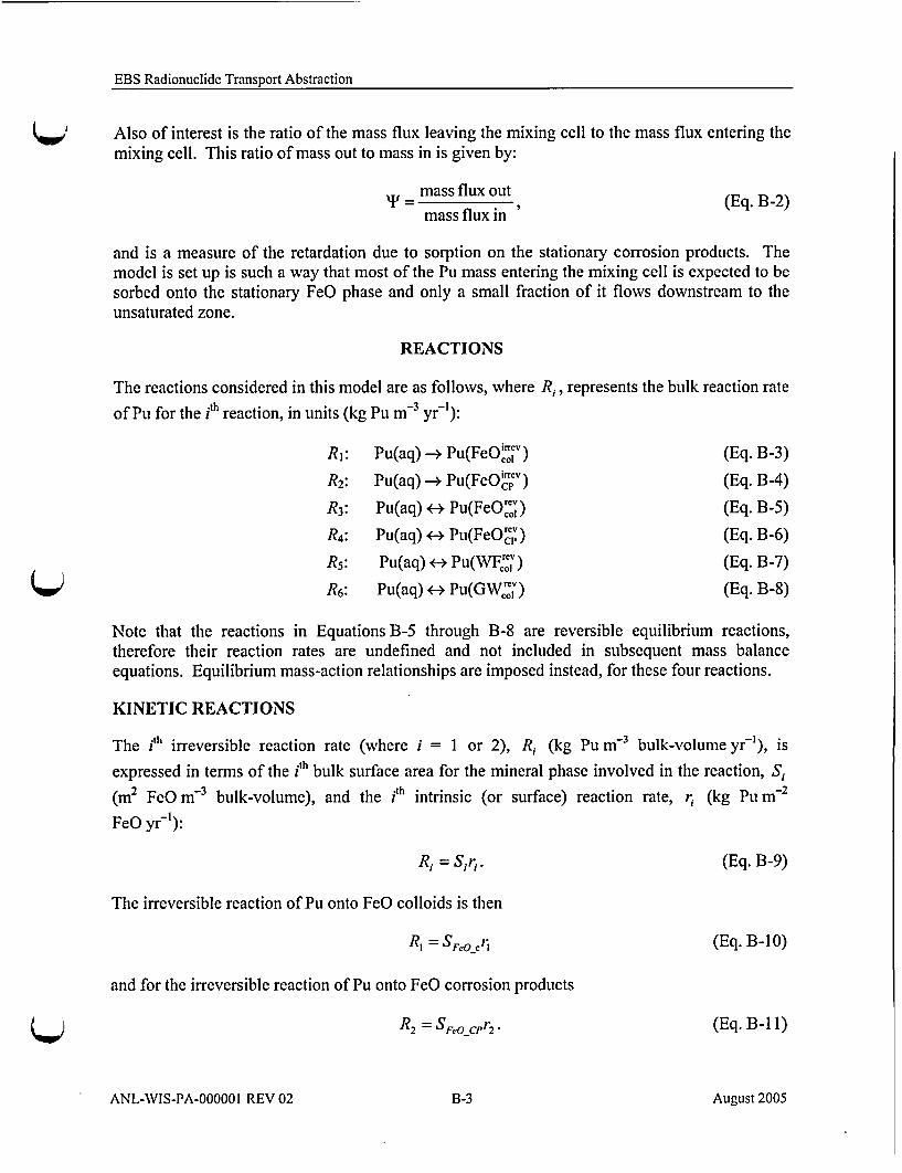
EBS Radionuclide Transport Abstraction
Also of interest is the ratio of the mass flux leaving the mixing cell to the mass flux entering themixing cell. This ratio of mass out to mass in is given by:
= mass flux out (Eq. B-2)mass flux in
and is a measure of the retardation due to sorption on the stationary corrosion products. Themodel is set up is such a way that most of the Pu mass entering the mixing cell is expected to besorbed onto the stationary FeO phase and only a small fraction of it flows downstream to theunsaturated zone.
REACTIONS
The reactions considered in this model are as follows, where R, represents the bulk reaction rate
of Pu for the iph reaction, in units (kg Pu m-3 yr-'):Rl: u~aq -+irrev
RI: Pu(aq) Pu(FeO"ot) (Eq. B-3)
R2: Pu(aq) - Pu(FeOp"') (Eq. B-4)
R3: Pu(aq) <-> Pu(FeO"') (Eq. B-5)
R 4 : Pu(aq) <- Pu(FeOc') (Eq. B-6)
Rs: Pu(aq) <-> Pu(WFfc'ý) (Eq. B-7)
R 6 : Pu(aq) <-> Pu(GWc,') (Eq. B-8)
Note that the reactions in Equations B-5 through B-8 are reversible equilibrium reactions,therefore their reaction rates are undefined and not included in subsequent mass balanceequations. Equilibrium mass-action relationships are imposed instead, for these four reactions.
KINETIC REACTIONS
The p1h irreversible reaction rate (where i = I or 2), R, (kg Pu m-3 bulk-volume yr-'), is
expressed in terms of the ith bulk surface area for the mineral phase involved in the reaction, S,
(in 2 FeO m-3 bulk-volume), and the ith intrinsic (or surface) reaction rate, r, (kg Pum-2
FeO yr-l):
R, = Sr. (Eq. B-9)
The irreversible reaction of Pu onto FeO colloids is then
Rg = Sreocr1j (Eq. B-10)
and for the irreversible reaction of Pu onto FeO corrosion products
R2 = SFeoCPr2 (Eq. B-11)
ANL-WIS-PA-000001 REV 02 B-3 August 2005

EBS Radionuclide Transport Abstraction
The bulk surface area (mi2 FeO m-3 bulk-volume) for FeO colloids and corrosion products are,respectively,
S Fec -2 S FeC cC FeC_c3
SFeOCP =" SFeOCPCFeOCP~Av
(Eq. B-12)
(Eq. B-13)
where 5 is the porosity of the FeO matrix, Sw, is the water saturation and
SFeo_C = specific surface area of FeO colloids (M2 FeO-colloid kg-' FeO-colloid)
SFeo-cp = specific surface area of FeO corrosion products
(m2 FeO-CP kg- FeO-CP).
The intrinsic or surface reaction rate (i.e., rate per unit mineral surface area) is considered to bethe same for the colloidal and stationary phases, i.e., r, =r2 -r, and it only has a forwardcomponent, since the reaction is irreversible. Further, suppose that the reactions are first order inthe solution concentration Cpu aq:
r = kCpu.q, (Eq. B-14)
where
k = forward rate constant, (m.3 water-volume m-2 FeO yr-).
The two irreversible reaction rates on a water volume basis are then
Ri ^-L. = SFeO cCFeO ckcpu_aq = Ricpuaq
R 2 = SFeO CPCFeO_CpkCpuaq = R2Cpuaq2OJS"
where R-1 = Seo_ CCFeO _k and R2 = SFeO _cpCreocpk are reaction
colloids and corrosion products, respectively.
(Eq. B-15)
(Eq. B-16)
rate constants (yf-1) for
EQUILIBRIUM REACTIONS
The four chemical species, Pu(FeO'v), Pu(FeOcv), pureWv',,,v) and Pu(GWrev)v, involved inreversible equilibrium sorption reactions, Equations B-5, B-6, B-7, and B-8, follow the law ofmass action according to
K>
ANL-WIS-PA-000001 REV 02 B-4 August 2005

EBS Radionuclide Transport Abstraction
,q [Pu(FeO[r')][Pu(aq)]
K =q [Pu(FeOc'p)][Pu(aq)]
Kq - [Pu(WloA)]K [Pu(aq)]
K = _ [Pu(GWVo•')]6 [Pu(aq)]
(Eq. B-17)
(Eq. B-18)
(Eq. B-19)
(Eq. B-20)
where [PuUj)] represents the thermodynamic activity of Pu in theyh phase (aqueous, colloidal, orcorrosion product). Normally, these relationships are expressed for dilute solutions as a simplelinear (Kd) (water volume/mass FeO) type of isotherm in terms of concentrations:
CpuFeOc = KdFeOCcCpuaq
CPuFeO CP = KdFeOCPCP._uaq
CPu WF c = Kd_ITcCpuaq
CPuGWI' c = Kd -G'cCPu aq
(Eq. B-21)
(Eq. B-22)
(Eq. B-23)
(Eq. B-24)
where
Cu-Feo-c = mass ratio of Pu sorbed onto FeO colloids (kg Pu kg-1 FeO-colloid)
Pu FeOCP = mass ratio of Pu sorbed onto FeO corrosion products (kg Pu kg-' FeO-CP)
C•-, PJc = mass ratio of Pu sorbed onto waste form colloids (kg Pu kg-1 WF-colloid)
Cp, GI1'r = mass ratio of Pu sorbed onto GW colloids (kg Pu kg-' GW-colloid).
The mass ratio for these reversible sorption reactions can be converted to water volumeconcentrations by the following:
CpuFeOc = CFeOcCCPuFeOCc
Cpu FeO CP =CFeOCPCpuFeO CP
CPu lit c = CGTcCCPuGIIFc
Cpu _GWl_ = CGWi~cCPu_Gil_c
(Eq. B-25)
(Eq. B-26)
(Eq. B-27)
(Eq. B-28)
The reversible Pu equilibrium is expressed by the partition coefficients relating the aqueous stateand the two reversible states given by Equations B-25 to B-28 as
CpuFeOc = CFeocKdFeOcCpu_aq = KdFeoc C Puaq (Eq. B-29)
ANL-WIS-PA-000001 REV 02 B-5 August 2005

EBS Radionuclide Transport Abstraction
Cp u_FeO_CP = CcFeO_CpKdFeOCpCpuaq = Kd_FeOCpCpu_aq (Eq. B-30)
Cpu Fc =CWVF cKdWF cCpuaq -Kd WIF cCpu_aq (Eq. B-31)
CPU GWc C=COWcKd G1VcCpuaq = KdGVcCPuaq (Eq. B-32)
where Kd_Feo c, KdFeOCp, Kd_WF,,_, and KdGIV_ are dimensionless partition coefficients.
QUANTIFICATION OF CORROSION PRODUCTS
The corrosion products are generated from the degradation of the waste packages. It is thecorrosion product mass that provides the porous matrix for the transport of radionuclides in thereaction mixing cell. The amount of corrosion products is time dependent. As modeled, thecorrosion product density (kg m-3 solid) and mass (kg) are known. Let
PFCO ~c = corrosion product density
mFeo-cp = mass of corrosion product.
The volume of corrosion products (m- 3 solid) is then
VFeOCPmFe cp- P PFeO_ CP
If the porosity of the corrosion product mass is specified as
V
Vbulk
then
VFeO _ CP
Vbulk
The bulk volume is computed from
bulk - VFeO CP
1-0
The pore volume is
Vpore = AVbulk _ nPFeO_CP
1- 0 P&~o-cp
ANL-WIS-PA-00000I REV 02 B-6 August 2005

EBS Radionuclide Transport Abstraction
and the water volume is:
V1.ater = SVpore = Sw Vbulk
The stationary corrosion products concentration is defined as
mFeo CPC FeO CP = te
TRANSPORT EQUATIONS
The mass balance equation for the Pu contained in the aqueous state, the reversible colloid stateand the reversible corrosion product state with radionuclide decay (neglecting ingrowth) is (seedevelopment in Section 6.5.1.2 culminating in Equation 6.5.1.2-46):
a.Sw (Cpu aq + Cpu _FeO c +•CPu FeO CP +-CPuuWFc + "u-GiWc
ata(Cpu-_q + Cpu FeO c + Cpu_1Fc + CPu G il c) _'a (_ .D aq aCpu-aqc
ax ax ax
(OS'c. (P e + CA, 11T c + Chg GI c
axe- c ax ) (Eq. B-33)
=-R 1 - R 2 - VS,(CPu aq + CPu_FeOc + CpuFeO_CP + CpJIrFc + CIV"c)
where 0 is the porosity of the FeO matrix, S,. is the water saturation, u is the Darcy velocity of
the water (m yr-), Daq is the diffusivity (mi2 yrl) of the Pu in solution, Dolloid is the colloid
diffusivity (M2 yr-), and 2 is the radionuclide decay rate (yf-'). Now impose the reversibleequilibrium of the Pu mass between the aqueous, colloid and corrosion products (Equations B-29through B-32) together with representing the irreversible reactions as functions of the aqueousphase Pu concentration (Equations B-15 and B-16). The mass balance (Equation B-33) on a bulkvolume basis can be expressed in terms of the concentration in the aqueous state:
ANL-WIS-PA-000001 REV 02 B-7 August 2005

EBS Radionuclide Transport Abstraction
(1+gd FeO c +Kd_FeOCP + KdW1F c +Kd GV- ) a)SwCP.u-aq_ at
+ 1+ KaFeO c + KdWF_c
ax ( wD a C pu aq "
ax- ax)
aCpu aq+Kdo, ac)x
(Eq. B-34)
ax-WFc - acpuaq+ +ax
-Os wS(R 1 + -2)Cpu _aq
-2A•S(1 + gdFeO-c + KdFeOCP + KdI,_I'F• + Kd-G1i c)Cpuaq.
Based on Equations 6.5.1.2-47 and 6.5.1.2-48, the mass balance equations for the irreversible Puin the colloid and corrosion product states are, respectively,
O•Swclr Pu FeC CO c ac k pP. &e c a( D ac P c+ _ _ _ OSwhDcotloid PuFex
at ax ax o axOSASRCp-a - 10wC lrrv Pu FeC c
aOSwc,Cr, Pu Feo CP
at - = SSwR 2Cpu aq -2 0SwCirrvPuFeOCP"
and
(Eq. B-35)
(Eq. B-36)
from left to
(Eq. B-37)
The boundary conditions require the upstream (left boundary cell, if flow isright) conditions
Cpuaq - Cs
CPu lt -c =Kd AIT CCs
CpuFeOc = CpuFeOCP =- Cirrv PuFeOc = Clrrv Pu FeOCCP = CPuGW 'c- O, (Eq. B-38)
where c, is the Pu solubility as defined earlier. In this model, no FeO or groundwater colloidsexist in the upstream waste form cell. The solubility at the upstream location is dependent on theCO2 fugacity and pH at the upstream location (BSC 2005 [DIRS 174566], Section 8.1) and ingeneral is time dependent: c, = c, (t). The right boundary cell is a free flow boundary withconcentrations fixed at zero for the purpose of this appendix. For diffusion calculations it isrequired to specify down stream diffusion parameters (porosity, diffusivity, diffusive length anddiffusive area). The initial conditions within the mixing cell are zero for all Pu concentrations.
Both the colloid and corrosion product concentrations are chosen to be time dependent:
ANL-WIS-PA-000001 REV 02 B-8 August 2005

EBS Radionuclide Transport Abstraction
CFeOc = CFeOc (t)
CFeO-Cr = CFeO-_L') (Eq. B-39)
CH-c_ = CIFTc (t)
cGI-c = CGaIV(t)
but are independent of the Pu concentrations. This implies that the reaction rates R, and R 2 arealso time dependent.
The mass balance equations are solved numerically by a finite difference method. Thecalculation sequence for a time step is to solve Equation B-34 for cp, aq. Reversible equilibrium
Equations B-29 through B-32 then give cp,_ Feo c, cPU_ FeoCP, CP', w-c and cP,,, wG I. With
cpa_.q known the mass balance Equations B-35 and B-36 for the irreversible components
are solved.
DIMENSIONLESS FORM OF TRANSPORT EQUATIONS
In order to express the governing equations in dimensionless form, dimensionless length, timeand concentration, respectively, are defined:
Z =x/L
itt ttt
OZSSWL LcawL
"C = C]Cs ,
where L is the characteristic length (in) and F = - is the average linear advective velocityOS.(m y-l). The characteristic length would be the interval length or, for a finite differencesolution, the grid block cell length. Then the variables are changed to dimensionless space andtime in the mass balance equations. If the colloid/corrosion product concentrations are taken tobe constant (Equations B-39), then the Pu mass balance equation in the aqueous state is:
(I+Kd_ Feo +'+Kd F CP +KdIcKdV) ar+(l+K---oc +K-'h'F c +K--- _ )aPuaq
+" (a(Eq. B-40)
[Aaq- Acolloid(Kd_FeO_c-Kd + Fd ¢"Kd GIIrc )]j" _ ua
S--(+O E) 2) Cpu _oq -(I + X--FeO-c + Td X-FO-- CP + d--_,ITc + KdF._ a )A'p_
ANL-WIS-PA-000001 REV 02 B-9 August 2005

EBS Radionuclide Transport Abstraction
where
Daq
A aq -
L
D colloid
Acolid -- L?
L
diffusive rate in wateradvective rate
diffusive rate of colloidsadvective rate
(Eq. B-41)
(Eq. B-42)
ii
L
k2102 =-
L
reaction rate to colloidsadvective rate
reaction rate to corrosion products
advective rate
(Eq. B-43)
(Eq. B-44)
2A
L
decay rateadvective rate
(Eq. B-45)
The dimensionless form of(Equations B-35 and B-36) are:
the mass balance for the irreversible Pu concentrations
O~hv P FO caEIrrv Pu FeO cJ rr p0 Fe + a - - A colloid
02F~rP Foc
(Eq. B-46)
=01cp._a,- A'F1• .rrvPuo
auCPrr_ Pa FeOCP
J'= 0
2 "Pu-aq- A-irrv"puFeo_CP" (Eq. B-47)
DIFFERENCE SOLUTION OF TRANSPORT EQUATIONS
Consider a finite difference approximation of the governing mass balance equations. Thediscretization uses three spatial cells. The left or first cell represents the upstream boundaryconditions. The second cell represents the mixing cell with reactions. The third or right cellrepresents the down stream boundary conditions. Since cells one and three represent boundaryconditions, this discretization is a 0-dimensional or single cell representation of the processes.Let the time step length be At. Let superscript n denote the nth time step, for example, c",,_.q
denotes the concentration at the nth time step. The discretization uses a first order backwarddifference approximation for the time derivative and the advective transport term. The diffusive
ANL-WIS-PA-000001 REV 02 B-10 August 2005

EBS Radionuclide Transport Abstraction
flux uses a second order approximation. This discretization is consistent with GoldSim(GoldSim Technology Group 2002 [DIRS 160579]). In this model, diffusion of dissolved massand waste form colloids occurs at the left boundary. At the right boundary, diffusion of bothdissolved mass and all colloids occurs. In addition, the porosity and water saturation are time-independent but may vary spatially. If the discretization is fully implicit in concentrations andtime dependent velocity, irreversible reactions and solubility, then the discrete form ofEquation B-34 for cell 2, in units of mass per unit water volume per unit time, is:
n+l n- Cpuaq Cpuaq +. ' ."n+17" n+l u ( n+1 7f q - C n a
I At 2Cpu_aq- (+Kd_WFjc•s -- left_aq Cs - Pu-a j
f ]- ( n+I _ .n+I . -ig co id Iright_aqCPu_aq -D _ IIOWdKd A'F Cs Cpu aq,)+ Tright-.ol6idE3Cpu aq
I + I P+1uaq
This equation is solved for c"_q , resulting in:
n+I
Cpuaq -
KICPu_aq "[- '(+ Kd_W1_¢ )AT + 1aq + -lefi colKd F c ]ýSAt
K.(U"n+l.k2 DlDefaq +Dleft c olKd_ Fc +_Dright aq + Dright_colK 3 + 2 T1n+.+RgI+.. t
(Eq. B-48)
where
uAt UAt = UAt•)S .L V,..ate
is the Courant number (dimensionless), L is the characteristic length (m), V.',Ir is the volume of
water in the cell (mi3 ), U is the volumetric water flux (M 3 yrl), and U is the advective rateconstant (yr-). Further,
Ko ,,+K F +Kd- c+K
K2 =l+dFeO-c +KdII'Fc +KdGJc
K3 = Kd FeO-c+Kd II'FcKdGJ-
and
V.,ater
ANL-WIS-PA-000001 REV 02 B-1II August 2005

EBS Radionuclide Transport Abstraction
is the diffusive rate constant (yFr) with respect to either the solution or colloid mass at either theright or left cell interface. Here, A., is the cross sectional area for diffusion (mi2). Fordetermining the diffusive rate constant for a finite difference approximation to the transportequations, the condition imposed is that the flux across the interface of two adjacent cells becontinuous at the interface. The resulting analysis gives the diffusive rate constant between two
cells as the harmonic average of or H( WDJ, which guarantees the continuity of theL L
diffusive flux at the cell interface. In general, the harmonic average of two numbers is:
2H(x, IX2)= 2
XI X2
For a finite difference approximation in which the cell lengths are Ax, and Ax2 , the harmonic
average of OS'D across the Cell I/Cell 2 interface is:Ax
Ax)I X 2 & +Ax A2
015 .IDI 0 2S.,2D21
Ll L2
01S., D, 02S.,2D2
where LZ and L2 are the half-lengths (m) of Cells I and 2, respectively. The diffusive rateconstant subscript left or right refers to the left or right diffusive boundary conditions, while thesubscript _aq or _c refers to diffusion of the dissolved mass or colloid mass, respectively.
The reversible concentrations are determined from Equations B-29 through B-32
-17+1CPU FeOc = drFeOc Pu1aq (Eq. B-49)
cn+l n+l
n+1 d,_OCPC~oO Pu_oq (Eq. B-50)
cn+l cn+I
CPUJ'Fc = Ed _ lIT (Eq. B-51)
cn+1 n+1CP1 UGil'c = Kd_G-_GIcPu_aq• (Eq. B-52)
ANL-WIS-PA-000001 REV 02 13-12 August 2005

EBS Radionuclide Transport Abstraction
The discretization of the balance Equation B-35 for irreversible Pu mass on the colloids yields
Cn "kn+l•t n+l
cn+ Clrrv_ Pu FeO c -I+ i tCpuaq1rv_P,_FeO_c =1 + (+ + D+ g1,it Co + 2)At (Eq. B-53)
and for irreversible Pu mass on the corrosion products, Equation B-36 yields
en n n+l
cn+l CIrrv Pu FeO CP + - 2ln+1puaq
Crv,_Pu_FeoCP - 1 + 2At (Eq. B-54)
SAMPLE CALCULATION WITH REPRESENTATIVE PARAMETERS
A sample calculation is performed to demonstrate the solution technique and illustrate the typesof behavior that might be expected in this model. Parameter values used in this samplecalculation are given in Table B-1. Let the solubility, flow velocity, and irreversible reactionparameters, which are actually time-dependent, be constant over time.
For this set of parameters, the irreversible reactive rates, advective rate, diffusive rates, decayrate and the dimensionless colloids and corrosion product partition coefficients are:
J? = 0.02000 yr"
R2 = 786 yr-'
U = 0.04367 yr-'
Dlef•_aq = 0.09127 yr"
Drightaq = 2.229 x10 3 yr
Drigh,_cot = 2.229 x 10⁻⁵ yr-1
2 = 2.875 x 10⁻⁵ yrl1
KdFeo-c = 0.20
Kd Feo cP = 1.965 x 10⁴
Kd_11Tv = 0.60
Kd -GI' = 0.020.
The simulation for the mixing cell (Cell 2) concentrations over a 1000-year time interval isshown in Figure B-2. The dominant rate constant, by several orders of magnitude, is the
irreversible rate constant of the corrosion products, R2 = 786 yr'. This is a result of the largemass of corrosion products and results in a relative large concentration of irreversibly sorbed Puon the corrosion products, Cr,,_Pu_FeOCP. For this simulation, the amount of corrosion product
mass is representative of the total mass of corrosion products in a waste package, and all thecorrosion products are available at initial time. In the TSPA-LA abstraction model, the corrosion
ANL-WIS-PA-000001 REV 02 B-13 August 2005

EBS Radionuclide Transport Abstraction
product mass is time dependent and a function of the corrosion rates for the carbon and stainlesssteel (see Section 6.5.3.2).
Another large mass of Pu is reversibly sorbed onto the corrosion products. This is a result of thelarge reversible partition coefficient for the corrosion products, Kd FeO CP = 19650, which again
is a result of the large corrosion product mass. For this simulation, almost all of the Pu mass issorbed onto the corrosion products either reversibly or irreversibly. Only a small amount ofmass remains in solution or is sorbed onto the colloids. The qualitative behavior of theconcentrations in Figure B-2 shows the concentrations approach a limiting value, with theexception of the irreversibly sorbed mass on the corrosion products. This behavior is discussedin the next section, where the concentrations are expressed analytically as solutions of differenceequations, and their asymptotic-in-time values are determined.
Table B-1. Representative Parameter Values for Sample Calculation
Parameter Value Units Description
C, 1.0 mg 1-1 Solubility
Sw 1.0 dimensionless Water saturation
A6 1.0 dimensionless Porosity of Cell 1
02 0.4 dimensionless Porosity of Cell 2
03 0.3 dimensionless Porosity of Cell 3
U 0.1 m3 yr-1 Volumetric water flux
Kd FeoGc 1 x 10⁴ ml g-1 Colloid partition coefficient
Kd Feo CP 2.5 x 10' ml g-I Corrosion product partition coefficient
Kd _IT-c 2 x 10' ml g-1 Waste form colloids partition coefficient
1ml Groundwater colloids partitionKd c 2 x 1mg- 1 coefficient
S Feoc 100 m2 g- Specific surface area of FeO colloids
SFeO CP 10 m2 g-1 Specific surface area of FeO corrosion________10___9_ productsCFeO-c 20 mg 1-1 Concentration of FeO colloids
CFeO CP 7.86 x I0o mg 1-1 Concentration of FeO corrosion- 7products
CVF-c 3.0 mg 1-1 Concentration of waste form colloids
CGwIc 0.1 mg 1-1 Concentration of groundwater colloids
k 0.001 cm yr-1 Forward sorption rate constant
V.,ater 2.290 m3 Water volume (= pore volume sinceS=1)
A'12 36.0 m2 Diffusive area between Cell I and Cell2
-,23 1.068 m2 Diffusive area between Cell 2 and Cell3
ANL-WIS-PA-000001 REV 02 B-14 August 2005

EBS Radionuclide Transport Abstraction
Table B-1. Representative Parameter Values for Sample Calculation (Continued)
Parameter Value Units Description
Li 0.001 m Half-length of Cell 1 diffusive path
L2 5.0 m Half-length of Cell 2 diffusive path
L3 0.806 m Half-length of Cell 3 diffusive path
Daq 2.3 x 10⁻⁹ m2 s-1 Aqueous diffusivity
Deoltoid 2.3 x 10⁻¹¹ m2 s-1 Colloid diffusivity
A 2.875 x 10⁻⁵ yr- 1 Radionuclide decay rate
E
0
0
0
1.OE+00
1.0E-01
1.OE-02
1.OE-03
1.OE-04
1.0E-05
1.OE-06
1.OE-07
1.OE-08
1.OE-09
0 100 200 300 400 500
Time [yrs]
600 700 800 900 1000
Figure B-2. Concentrations with Respect to Water Volume
CLOSED FORM SOLUTIONS OF THE DIFFERENCE EQUATIONS
If the solubility, advective flux, saturation, and irreversible rates are chosen to be constant overtime, then the mass balance equation for the aqueous Pu, Equation B-48, is a first order linearconstant coefficient nonhomogeneous difference equation. This equation is of the form
Cn<aq = alc, .q n +a 2 (Eq. B-55)
ANL-WIS-PA-000001 REV 02 B-15 August 2005

EBS Radionuclide Transport Abstraction
where
K k+(UK=+ Dlep_, + gleACOIK, 11,,'F c +Drightaq + DrighcoAK3 + k. + kR + 'i Pt
(U (I + Kd III' c) + DI1,_ aq + eft_ colkd_AF_c ý) C$K, _ + q + Dleftcol- Td _ + rightaq +rDigh, coKA + kR +A,)At
The difference equation (Equation B-55) with initial condition of zero concentration hasthe solution:
Cn - a 2 (1- a')pu_aq - -a- (Eq. B-56)
where a," is a, raised to the n'h power (i.e., not a, at time step n). Since the condition 0 < a, < 1is guaranteed (because all terms in the definition are positive, and the denominator is the sum ofthe numerator plus positive terms), the solution c"_aq for large time is asymptotic to:
lim C" a 2•l~m•Cp -aq la
(U(l+ 4-K====d 0 E c)+ 51ief, aq +D51,gftcolK==d WF c s (Eq. B-57)
U K 2 + DTh_+ o aq + DTfi COIKdJITc + Drigh,_aq + Dig,=_oII K +Rj +R2 +coKt
The terms in this expression represent the effects of advection, diffusion, decay, and reversibleand irreversible sorption reactions.
The difference equation for the irreversible colloid concentration (Equation B-53) is first orderlinear and is written as:
CJTVp_PFeOc_ = b3C 1rPu FeC c +b 2 ;:aq (Eq. B-58)
where
I + ( D--+ ri,_coI + 2 )At
b2 = 1hA t1 + (U+D5rig,;,co, + AA
(Eq. B-59)
(Eq. B-60)
andccp`".q is given by Equation B-56. The difference Equation B-58 with initial condition zero
has solution
ANL-WIS-PA-000001 REV 02 B-16 August 2005

EBS Radionuclide Transport Abstraction
a2b2 [1-b b+l' a' a+ - b,?+1- I- I
Irr c _ YFO_ -a, [- b1 a, -b,
Since 0 < a, < 1 and 0 < bi < 1, this solution has asymptotic behavior
a 2 b 2lim C"n_00- rvPuFe• (1-a,)(1-bl)
(Eq. B-61)
(Eq. B-62)
Thus
limc" Pu C I limc (Eq. B-63)Imcrr• o -b1 lcpuq U + Dright-cot +, 2 Puaq (
The difference equation for the concentration of the irreversible mass on the corrosion products
is first order linear and is written ascn+1 n Cn+l
Crr_Pu_FeOCP = elClrrV_PuFeO_CP + e2C Pu_aq (Eq. B-64)
where
1e, = + (Eq. B-65)
S=R2At (Eq. B-66)
If 2 > 0, Equation B-64 with initial concentration of zero has solution
a2e2 --e 1 (Eq. B-67)CIrrvPuFeo CP I-al [-e, a I-e, j
If 2 = 0, Equation B-64 with initial concentration of zero has solution
,, a2 e..__2 [1 a +PrvP,,_ = aCP = - [+ n+l1 . (Eq. B-68)__ 1-al Ia 1
The solution Equation B-67 has asymptotic value
P1 e2 .. ,, R2 MC(qB-9Pmc u_, P. FOCP = U lmc ,aq = Pu aq, (Eq. B-69)
n-im 1 I- e, n-+o A n -m "
whereas the solution Equation B-68 does not have a limiting value, but is unbounded as afunction of the time index n.
ANL-WIS-PA-000001 REV 02 B-17 August 2005

EBS Radionuclide Transport Abstraction
BOUNDARY FLUXES
Now consider the two boundary flux conditions given in Equations B-1 and B-2. The left orupstream boundary flux accounts for advection/diffusion of Pu mass in solution (Pu__aq) and Pumass sorbed to waste form colloids. In this section of the analysis, upstream diffusion of colloidsis ignored, although the TSPA-LA implementation does account for upstream colloid diffusion.The mass flux rates (kg yr-) at the upstream (left) boundary for the nth time step are:
AdvectivePu aq (kg yrl)
DiffusivePu aq (kg yFr)
AdvectivePuWF-c (kg yf-')
DiffusivePuWF c (kg yr-)
= V., c-water cs= -Dieft aqVwtater(Cs -Cpu~aq)
= U V..,,,.g ,,T IF:,
= Deft aVwt,,,,rKd., ,,T C (c- CPU-oq)
The right or downstream boundary flux has contributions from advection/diffusion of Pu insolution and colloid together with advection/diffusion of IrrvPu on colloids. There is noadvective or diffusive flux associated with the immobile corrosion products. The mass flux rates(kg yrl) at the right boundary assuming zero downstream concentrations are:
AdvectivePu aq (kg yr-')
DiffusivePu aq (kg yr'-)
AdvectivePuFeO-c (kg yr-)
Diffusive Pu FeO-c (kg yFr)
AdvectiveIrrvPuFeO_c (kg yr-)
DiffusiveIrrvPuFeOc (kg yf')
AdvectivePuWF-c (kg yr'l)
DiffusivePuWF-c (kg yr-)
AdvectivePuGW-c (kg yr1)
Diffusive Pu GW.c (kg yr-)
= right aq waterCpu aq
watr dFeC~CPu aq= ni',.Y K~ p• Cn
= Dright colVtwaterS_ Feo_c Pu_aq
UVwater Jrrv Pu FeOCc
Dright-col ViierCyPu_ FeO-c
= UV waterk , _CPu_oq
= UV..~.aerKdG,. "CCnaq
"DrightcolVuwaterkd _ _ ucCuaq
The total flux at the left boundary (upstream) at the nth time step, Flefibddy total' 1i
Flef total '=- U VwaterCs + Alefteaq P _btr(tot aq)
+UVJ,.aterKd*5 WFcCs + Dieft co.V..aerKd_,,'_ -cuaq)
ANL-WIS-PA-000001 REV 02 B-18 August 2005

EBS Radionuclide Transport Abstraction
The condition discussed in Equation B-i considers the ratio of the colloid mass to total mass fluxout the right boundary. The right boundary colloidal flux, Frngh, bdCOlloid, due to both reversibly
and irreversibly sorbed Pu is:
Fright_bdadycolaoid "': d FeO T cCpu-aq + U aterClrrvPuFeO-c
+UVu-aterKd_ J'Fc ',, c q +UV,,.aerKdq I aPe,_aq
+K
CX+
u
right col Vwaterkd FeO cCunaq + DrigitcoVwaterClrrv_ O
C n Vl'jr d C
Dright coltVwaterKd_ UEcCpuaq + Drightcotl waterd_aGilCpuaq
The total Pu flux at the right boundary, Fr ght bddtotal,
Fr'igh,_bddoa F;, bd,.,od+•',~r•o -+right aqVwsaterCpnu aq"_F.h bd' to fat =F.ght bddy _colloid + UJVwaterCP~u aq + D i/t qVV1CCua
The right boundary ratio of colloid flux out to total flux out at time level n is
F nQ right _bdMy _ colloid
F nright _bddy total
Then
n
K 3 +.C lrv-<u-FeC cnPu-aq
U K2 + Drigh, aq + Aright colgK3 Clrrv PuFeO-c+ -• n
U + DBrightcol Cpuaq
Now from Equation B-63
liCI~rn Pu FeC c Rlim Cr•WrO° - -
Cpu_aq U + Dright col +2
The limiting value for the right boundary ratio of colloid flux to total flux is
K32U + Dright _col +K2 = lim g2 ,, = - ---n- U K 2 + Dright aq + Dright col K 3 -RI
Drightcol U + DrihgcoI + A
or
ANL-WIS-PA-000001 REV 02 B-19 August 2005

EBS Radionuclide Transport Abstraction
Uih C0 +2)+igh oC U K= + rgta Dih U +Dright col + 2. "1 (Eq. B-70)(UK2 +ADig,,,_oq +5DL.,h,_COX3 -: - ,_o_. + A.U + Dright CoI )
This can be written as
0 = .P + k' (Eq. B-71)P 2 +Rk
where
p, = K3 P + rioh, -col +2)
P2 =(UK 2 +rightaq + rigt c + rc +U + Dight-co
Note the limiting flux out ratio 92 satisfies
K0U (U +5 righ, coi)0 <__ - - _ <n<1,U K2 + Dright _ aq + Drigit, - colK 3
where the lower bound on 92 is obtained when R1 = 0. Qualitatively, if the advective, diffusive,
and decay rates dominate the reactive rate constant RI, then K2 is close to the minimum value.However, if the reactive rate constant dominates, then 02 is close to one. The latter is theexpected qualitative behavior of the system as alluded to in the introduction of this appendix.For the parameter values given in Table B-1, the minimum value f = 0.4384 is obtainedwith Ri = 0.
The limiting flux out ratio for Table B-I parameter values (Rk = 0.02 yr"') is L2 = 0.5487; inother words, about 55% of the total Pu mass exiting the cell is sorbed onto colloids. Figure B-3shows the dependence of the flux out ratio E2 on the irreversible linear reaction rate constant k,
where k, = S Fo cCreo ck. The 92 value point obtained with the Table B-1 parameter values is
also shown in Figure B-3. An increase of the irreversible linear reaction rate, k, ofapproximately one and a half orders of magnitude would increase the flux out ratio toapproximately 95%.
ANL-WIS-PA-000001 REV 02 B-20 August 2005

0EBS Radionuclide Transport Abstraction
In the expression for irreversible sorption to colloids, R, = SFeo_ CFeo ck, consider theirreversible linear reaction rate k a fitting parameter to match a specified flux out ratio 0. Thenthe solution of Equation B-71 for k is:
k P2( - Pl(I - n•)SFeo c CFeO c (Eq. B-72)
The result in Equation B-72 provides the fitting parameter, k, given a target flux ratio Q. Fromthe parameter values in Table B-I and with Q = 0.95, the irreversible linear reaction rate isdetermined from Equation B-72 as k = 0.04184cm yr-1 . The fitting parameter curve togetherwith this point is shown in Figure B-4.
1.0
0
cc
0
.9d-
0.8
0.6
0.4
0.2
0.0 11.E-05 1.E-04 1.E-03 1.E-02 1.E-01 1.E+00
Irreversible Linear Reaction Rate [cm yr-]
Source: Worksheet: K-surface in Appendix F.
Figure B-3. Limiting Flux Out Ratio, K2, as a Function of Irreversible Reaction Rate
ANL-WIS-PA-000001 REV 02 B-21 August 2005

EBS Radionuclide Transport Abstraction
- 1.E+00
E- Irreversible Rate• 1.E-01 . Fitting Curve
o = 0.950
1.E-02
1.E-03
• 1.E-04
0.4 0.5 0.6 0.7 0.8 0.9 1.0
0, Colloid Flux to Total Flux Ratio
Source: Worksheet: adv diff decay in Appendix F.
Figure B-4. Linear Reaction Rate from Colloid to Total Flux Out Ratio, 0
The ratio of the total flux out (right boundary) to total flux in (left boundary) at time step n is
T (UK2 + Dightaq + Drght_,clK 3 ýPnu aq + (U + Dight _co )Co rvPuFeO-c
(U0(+ Kd WF c)+ Okftaq + Oleft cogkd _ WF c ýs -(-Deft_ aq + 5,lef, colkd WF c Fu_caq
The numerator and denominator in this expression are divided by c' aq' and the limit is taken as
n goes to infinity. Equation B-63 implies:
lim rr Pu FeO c__
Pu_ aq U+ Dright_ col +
Denote
U + ±Brig2co + 2
U+ Dright _ col
and multiply the numerator and denominator of the equation for Tn by Z. The numerator
reduces to P 2 + R1. Now consider the denominator term multiplied by Z. It follows from
Equation B-57 that
ANL-WIS-PA-000001 REV 02 B-22 August 2005

EBS Radionuclide Transport Abstraction
(U0 + Kd-1_.-)+ A-,T,1 +le co, -TdIF) jrnlim eP"u_aq
=UK2 + Diefiaq + DOeft cot Kd_1F_c +Drig, t_aq +DrighIcoIK3 + Rj +R 2 +2K-?K
Therefore, the denominator is calculated as
[UK2 + flf._q + Dief, cot• _JIT_c + Drigu,_aq + righ,.co1K 3 + -+ k + (1-,ef - q+Dle,coKdI•c)j
= [UK-2 + Dightaq + DrightogK3 + R,-+ k 2 + -I-
=P2r( U + D ,co, + N +(4=P+ U+D +2 '•-+u+Dright coI
The limiting flux ratio then has the limiting value:
T = P2 +(Eq. B-73)r•+ U + ••- • Argh _+ -co-tP2 +[Uiý h~~ ](-+k2
The mass flux ratio TP is calculated from Equation B-73 for the Table B- 1 parameter values, butwith irreversible linear reaction rate k = 0.04184 cm yr- obtained from the fit to f = 0.95.Equation B-73 gives:
T= 1.293 x 10⁻⁴,
which demonstrates that most of the Pu mass is reacted both reversibly and irreversibly to thecorrosion products.
CONVERGENCE ESTIMATES FOR CLOSED FORM SOLUTIONS
Consider the convergence of the concentration in the aqueous state given by Equation B-56:
C pu-aq -- 1-a
with limit value (Equation B-57)
limc Puaq " a2n-m Ptt~1 I-a,
ANL-WIS-PA-00000I REV 02 B-23 August 2005

EBS Radionuclide Transport Abstraction
The relative error estimate with tolerance c is given by
h~mCpu aq • Cpu aq
limcn aqI --m. CPu _aq
Then the error estimate is
= a, <-.a2
I-a,
The bounds 0 < al < 1 implies log1 0 a, < 0 and the error estimate holds for
logio C
log1 o al
or
time =nAt > log°10 At.
log10 a,(Eq. B-74)
The time to converge to a given relative error tolerance for all reversible sorbed Puconcentrations is the same as the estimate for the aqueous concentration, inequalityEquation B-74, since the reversibly sorbed concentration is a constant multiple of theaqueous concentration.
Now consider the convergence of the irreversible Pu concentration on colloids, c, pu c. An
estimate of the relative error is given by
C.r, Pu .- . .i.MC .l Irrv -' u c
a2b2 Il- bln~ a?"~' -bn'l__1 1 a2b2
1-a,[1I-b1 a,-b 1 I (1-a.)(l-b1 )a2b2
(I (l~b) IbI an+i -bln+Il
I-, a ,-b ,
a-b 1 1
ANL-WIS-PA-00000I REV 02 B -24 August 2005

EBS Radionuclide Transport Abstraction
This estimate holds if
b n+,< aI -bI 6 and a+l< a,-b, C
1-a, 2 ' I-b, 2
These two estimates are satisfied if
n + 1_ Integer[maxl( loglb ' log'° a2 )] + I[ ,logo'b, I logio al
or
time = nAt >Ž ntege max/( -g10 b At. (Eq. B-75)S .logl0 b, 'lOglo a, )]
For a relative error tolerance of 1% (e = 0.01 ) and the parameter values in Table B-I, Figure B-5shows the time to converge for time step size 0.1 to 1000 years for both the aqueous Puconcentration and irreversible colloid Pu concentration. For example, if the time step is small,say 10 years, the number of years to converge within the given tolerance for the aqueous phaseconcentration is 137 years, whereas the time to converge for the irreversible colloidconcentration is 240 years. If the time step is increased to 100 years, then the time to convergeto the aqueous phase concentration is 286 years (three time steps), whereas the time to convergeto the irreversible colloid concentration is 500 years (5 time steps).
ANL-WIS-PA-000001 REV 02 B-25 August 2005

EBS Radionuclide Transport Abstraction
1.E+04
1.E+03 i__
0•
1.E+02 E "0U0
E -- 3 C Pu-aq
1.E+01<>c irrv Pu c,
I.E+001.E-01 1.E+00 1.E+01 1.E+02 1.E+03
Time Step Size [yrs]
Source: Spreadsheet: timetoconv.xls, Worksheet: plot time to conv in Appendix F.
Figure B-5. Time for Concentration to Converge with 1% Relative Error Tolerance
Appendix F presents the calculational spreadsheets that implement the equations inthis appendix.
ANL-WIS-PA-000001 REV 02 B-26 August 2005

EBS Radionuclide Transport Abstraction
APPENDIX C
MICROSOFT EXCEL SPREADSHEET "FLUX SPLIT DRIP SHIELD MODEL"
ANL-WIS-PA-00000I REV 02 August 2005

EBS Radionuclide Transport Abstraction
ANL-WIS-PA-00000I REV 02 August 2005

EBS Radionuclide Transport Abstraction
MICROSOFT EXCEL SPREADSHEET "FLUX SPLIT DRIP SHIELD MODEL"
SPREADSHEET "FLUX SPLIT DRIP SHIELD MODEL" WORKSHEET"F CALCULATIONS"
A-
'-91
25
127
29
•'A __ Be Eh F FratHoI S e Lbeach Flow Fraction Calculaflo usinig Sinosh Drip Shield Data, On-Crown Tests
Somqe. Oatascigmad.WAIsigma. ealoated or, hu"SredAngs"shee I
Itk col test. comopmg Itso i.Yb.Yc.Ydwid~to.
r-,* OTN: MOO207EBSATBVP.623
a.Vertical
r. Drip OistacneLocation hoIsFletatly. Crown
to (drip to L Patch FlowBerach Top oF ba- Drip into
[rip Location Breach Ceomm. Breach wid Flea Broach(T-•t Oerrespo)a o (_.j (cm. (il.) (N) (9)V .1rl-r Tý011 4 _136.5 13.5 17682 22.02
5 0 86 t3.5 W6742A112
.5 4 I s 11305 133.79 9l 1
I . _ 4 0 13& _5 13.166•.63 22. 25
-.F_ Ptch 5 -27 6 t3.5 27&14 4.4927c Ra Scne 4 27 1365 135 276.63 2.63
-27 13. 13.5 22.22 3.45
5 27 es 13.5 221.12 3.54
4 0 136.5 13.5 337.72 46.41
fIo Flw RteToo) 4 0 1365 135 66669 76$827 cm W44 of DS9 corte,
4 27 M..5 135 33269 335
( 27 Rate Ts) 2"7 6$ 6.635
eu~~f~lFoRhte 5 -27 96 135 376.73 245center (LotFow FRate
"I Test] 5 -27 as 13.5 137472 445H- OTN: MMOO2S7SATSVP 025
DTN: MO0207EBSATBWP.023 [DIRS 163402]; DTN: MO0207EBSATBWP.024 [DIRS 163401];DTN: MO0207EBSATBWP.025 [DIRS 163403].
Figure C-1. Spreadsheet "Flux Split Drip Shield Model," Worksheet "f calculations;" Calculation ofExperimental Breach Flow Fractions and Model Flow Fractions for Mean Minus OneStandard Deviation Rivulet Spread Angle
The purpose of this spreadsheet is to develop the drip shield flux splitting submodel usingexperimental data from the breached drip shield experiments. The data are analyzed to estimatean average and range of the rivulet spread angle, a. The disparity between measured fraction ofdripping flux that enters a breach and the fraction calculated using the model (with the measuredrange of the rivulet spread angle) is then used to establish a range of uncertainty in the model.
All descriptions for this worksheet (Figures C-1 to C-4) pertain to Rows 9-22. Equations inspreadsheet format are illustrated using Row 9.
ANL-WIS-PA-000001 REV 02 C-1 August 2005

EBS Radionuclide Transport Abstraction
Column B:
Column C:
Column D:
Column E:
Column F:
Column G:
Drip location as indicated for each test in the designated DTN (Figure C-I).
Breach or patch number most pertinent to this particular test, for which flow isanalyzed in this row of the spreadsheet.
Drip location, y, relative to the center of the breach listed in Column C.
Distance along the drip shield curved surface, x, from the drip shield crown to thetop of the breach.
Half-width, t, of the breach (13.5 cm), same for all breaches.
Measured mass of water, F,, dripped onto the drip shield during the test. It is
assumed that half of the water that dripped onto the drip shield, F, /2, floweddown the side that contained the breach.
Measured mass of water, F2 , that flowed into the breach during the test.Column H:
Column 1: Fraction of water dripped onto the drip shield that flowed into the breach:
F2 2F2
, F/2- F,
19=H9*2/G9
Column J: x tan a, where x is from Column E, and a is the spread angle. For Columns J-X,the value used for a is 8.8708' (Cell $M$7), which is one standard deviation lessthan the mean measured spread angle for these tests (see Worksheet "Spreadangles").
J9=$E9*TAN(RADIANS($M$7))
€-
Column K: Case number as described in Sections 6.5.1.1.2.1 and 6.5.1.1.2.2. For Case 1,t > xtana; for Case 2, t < xtana ; x is from Column E, and the half-width of thebreach, f, is from Column F.
K9=IF($F9>J9,1,2)
Column L: Value of YA (Point A) as described in Sections 6.5.1.1.2.1 and 6.5.1.1.2.2,corresponding to the leftmost point from which the edge of the fan from therivulet can enter the left side of the breach:
YA4 =-t-(x+2t)tana
L9=-$ F9-($ E9+2*$ F9)*TAN (RADIAN S($M$7))
ANL-WIS-PA-000001 REV 02 C-2 August 2005

EBS Radionuclide Transport Abstraction
Column M: Value of YB (Point B) as described in Sections 6.5.1.1.2.1 and 6.5.1.1.2.2,corresponding to the leftmost point from which rivulets will enter the top edge ofthe breach. The value of yB depends on the Model Case number (Column K):
YB -f+xtana
YB =e-xtana
Case 1.
Case 2.
M9=IF(K9=1 ,(-$F9+$E9*TAN(RADIANS($M$7))),($F9-$E9*TAN(RADIANS($M$7))))
Column N: Value of Yc (Point C) as described in Sections 6.5.1.1.2.1 and 6.5.1.1.2.2,corresponding to the rightmost point from which rivulets will enter the top edgeof the breach. The value of Yc depends on the Model Case number (Column K):
Yc =e-xtana
Yc =-e+xtana
Case 1.
Case 2.
N9=IF(K9=1 ,($F9-$E9*TAN(RADIANS($M$7))),(-$F9+$E9*TAN(RADIANS($M$7))))
Column 0: Value of Y, (Point D) as described in Sections 6.5.1.1.2.1 and 6.5.1.1.2.2,corresponding to the rightmost point from which the edge of the fan from therivulet can enter the right side of the breach:
YD =f+(x+2eQtana
09=$F9÷($E9+2*$F9)*TAN(RADIANS($M$7))
Column P: Determines which region (designated as Fraction Case #) along the crown wherethe drip is located:
1. Y•YA
2. YA <Y<-
3. -t<Y<yB4. YB <Y<Yc
5. Yc <Y<f
6. f<Y<YD7. Y>YD
P9=IF(D9<=L9,1,IF(D9<=-F9,2,IF(D9<M9,3,IF(D9<=N9,4,IF(D9<F9,5,IF(D9<09,6,IF(D9>=09,7)))))))
ANL-WIS-PA-000001 REV 02 C-3 August 2005

EBS Radionuclide Transport Abstraction
411~~~~ , Ký L ýO R SL 'I Crown Tests This ,celperfmsi a
The Ispread angl es are the rmean. I- cofldkit4io test. comopafnng This ccl IS the Iv alue3 sigma. and I.sigma. c•lated on the . ..YYb. Yo. Yd. and Ito detetmined by the
"Spread A.nges" she determine which case applies appropriate case oi the7
-4
13
120
. J2'
Figure C-2. Spreadsheet "Flux Split Drip Shield Model," Worksheet "I calculations;" Calculation of ModelFlow Fractions for Mean Minus One Standard Deviation Rivulet Spread Angle
Columns R though X (Figure C-2) compute the fraction of dripping flux f,1~ that is predicted toflow into a breach, assuming the drip location is within each of seven regions along the crown.Although fac,, is computed for all seven regions, it is valid in only one of the regions. Thecorrect valid region is determined in Column P (Fraction Case #), and the appropriate value fromColumns R through X is entered in Column Q.
Column Q: fcaic is the fraction of dripping flux onto the drip shield that is predicted by thedrip shield flux splitting submodel, Equations 6.5.1.1.2-2 through 6.5.1.1.2-6or 6.5.1.1.2-19 through 6.5.1.1.2-23, for Cases 1 and 2, respectively. f~1• isintended to be compared with f,,p, (Column I). The value of f,,,ai is selected from
Columns R through X, depending on the appropriate Fraction Case # (Column P).
Q9=IF(P9=1,R9,IF(P9=2,S9,IF(P9=3,T9,IF(P9=4,U9,I F(P9=5,V9,IF(P9=6,W9,1F(P9=7,X9)))))))
ANL-WIS-PA-000001 REV 02 C-4 August 2005

EBS Radionuclide Transport Abstraction
Column R: Value of fcaic in region 1 (y < YA), where fcaic = 0.
R9=0
Column S: Value of fcaic in region 2 (YA <y_< -0):
fcaic = y+f+(x+2t)tana2(x+2e)tana
S9=(D9+F9+(E9+2*F9)*TAN(RADIANS($M$7)))/
(2*(E9+2*F9)*TAN(RADIANS($M$7)))
Column T: Value of fcic in region 3 (-f<Y<YB):
2y++xtanafcalc = 2x tan a
T9=(D9+F9+E9*TAN(RADIANS($M$7)))/(2*E9*TAN(RADIANS($M$7)))
Column U: Value of fcic in region 4 (YB < y < Yc):
20L alc =-2
2xtan a
U9=IF(K9=1, 1,(2*$F9/(2*$E9*TAN(RADIANS($M$7)))))
Column V: Value of fcaIc in region 5 (yc < y < f):
f - y ++ x tan af.Ic = 2x tan a
V9=(-D9+F9+E9*TAN(RADIANS($M$7)))/(2*E9*TAN (RADIANS($M$7)))
Column W: Value of fc1• in region 6 (0• <Y < YD):
fl-- y+ 0+(x + 2)tan a2(x + 2e tan a
W9=(-D9+F9+(E9+2*F9)*TAN(RADIANS($M$7)))/(2*(E9+2*F9)*TAN(RADIANS($M$7)))
Column X: Value of f.,Ic in region 7 (y > YD) where fc,,ic = 0:
X9=0
ANL-WIS-PA-000001 REV 02 C-5 August 2005

EBS Radionuclide Transport Abstraction
45
-.
; an AsAP_ AE AF L 8 A; A:AJ AK-- AýL- WAM
S
$
10
ii
12
13
14
15
16
17
18
19
21
22
Figure C-3. Spreadsheet "Flux Split Drip Shield Model," Worksheet "f calculations;" Calculation of ModelFlow Fractions for Mean Rivulet Spread Angle
Columns Y though AM (Figure C-3) repeat the calculations done in Columns J though X usingthe mean rivulet spread angle of a = 13.1527 0 (Cell $AB$7). For Row 9, the spreadsheetequations are as follows:
Y9=$E9*TAN(RADIANS($AB$7))
Z9=IF($F9>Y9,1 ,2)
AA9=-$F9-($E9+2*$F9)*TAN(RADIANS($AB$7))
AB9=I F(Z9= 1 ,(-$F9+$E9*TAN(RAD IANS($AB$7))),($F9-$E9*TAN(RADIANS($AB$7))))
AC9=I F(Z9= 1 ,($F9-$E9*TAN(RADIANS($AC$7))),(-$F9+$E9*TAN(RADIANS($AB$7))))
AD9=$F9+($E9+2*$F9)*TAN(RADIANS($AB$7))
AE9=IF(D9<=AA9,1,lF(D9<=-U9,2,IF(D9<AB9,3,IF(D9<=AC9,4,IF(D9<U9,5,iF(D9<AD9,6,iF(D9>=AD9,7)))))))
AF9=IF(AE9=1 ,AG9,IF(AE9=2,AH9,IF(AE9=3,AI9,IF(AE9=4,AJ9,1F(AE9=5,AK9,IF(AE9=6,AL9, I F(AE9=7,AM9))))))) 0
ANL-WIS-PA-000001 REV 02 C-6 August 2005

4
EBS Radionuclide Transport Abstraction
AG9=0
AH9=(D9+F9+(E9+2*F9)*TAN(RADIANS($AB$7)))/(2*(E9+2*F9)*TAN(RADIANS($AB$7)))
A19=(D9+F9+E9*TAN(RADIANS($AB$7)))/(2*E9*TAN(RADIANS($AB$7)))
AJ9=IF(Z9=1, 1,(2*$F9/(2*$E9*TAN(RADIANS($AB$7)))))
AK9=(-D9+F9+E9*TAN(RADIANS($AB$7)))/(2*E9*TAN(RADIANS($AB$7)))
AL9=(-D9+F9+(E9+2*F9)*TAN(RADIANS($AB$7)))/
(2*(E9+2*F9)*TAN(RADIANS($AB$7)))
AM9=0
Columns AN though BB (Figure C-i) repeat the calculations done in Columns J though X usinga rivulet spread angle of a = 17.2903 0 (Cell $AQ$7), which is one standard deviation greaterthan the mean rivulet spread angle. For Row 9, the spreadsheet equations are as follows:
AN9=$E9*TAN(RADIANS($AQ$7))
A09=IF($F9>AN9,1,2)
AP9=-$F9-($E9+2*$F9)*TAN(RADIANS($AQ$7))
AQ9=IF(AO9=1 ,(-$F9+$E9*TAN(RADIANS($AQ$7))),($F9-$E9*TAN(RADIANS($AQ$7))))
AR9=IF(AO9=I ,($F9-$E9*TAN(RADIANS($AQ$7))),(-$F9+$E9*TAN(RADIANS($AQ$7))))
AS9=$F9+($E9+2*$F9)*TAN(RADIANS($AQ$7))
AT9=IF(AH9<=AP9,1,IF(AH9<=-AJ9,2,IF(AH9<AQ9,3,IF(AH9<=AR9,4,IF(AH9<AJ9,5,IF(AH9<AS9,6,IF(AH9>=AS9,7)))))))
AU9=IF(AT9=1,AV9,IF(AT9=2,AW9,1F(AT9=3,AX9,IF(AT9=4,AY9,IF(AT9=5,AZ9,IF(AT9=6,BA9,IF(AT9=7,BB9)))))))
AV9=0
AW9=(D9+F9+(E9+2*F9)*TAN(RADIANS($AQ$7)))/(2*(E9+2*F9)*TAN(RADIANS($AQ$7)))
AX9=(D9+F9+E9*TAN(RADIANS($AQ$7)))/(2*E9*TAN(RADIANS($AQ$7)))
AY9=I F(AO9=1,1 ,(2*$F9/(2*$E9*TAN(RADIANS($AQ$7)))))
AZ9=(-D9+F9+E9*TAN(RADIANS($AQ$7)))/(2*E9*TAN(RADIANS($AQ$7)))
BA9=(-D9+F9+(E9+2*F9)*TAN(RADIANS($AQ$7)))/(2*(E9+2*F9)*TAN(RADIANS($AQ$7)))
BB9=0
ANL-WIS-PA-000001 REV 02 C-7 August 2005

EBS Radionuclide Transport Abstraction
Figure C-4. Spreadsheet "Flux Split Drip Shield Model," Worksheet "I calculations;" Calculation of ModelFlow Fractions for Mean Plus One Standard Deviation Rivulet Spread Angle
Rivulet spread measurements are listed in Column D, Rows 6-31 (Figure C-5), for 26 testsdescribed in the indicated DTNs. The sketch to the right shows the relationships betweenmeasured rivulet spread ("1/2 spread") and the "1/2 spread angle," a. The average, pr, ofthe 26 spread measurements (Cell D33) is 20.096 cm, with a standard deviation, ca, of 6.674 cm.The uncertainty in the spread angle is incorporated into the drip shield flux splitting submodel byassigning a range for the rivulet spread of/fir ± lo-. The mean rivulet spread and pr ± Ilo areshown in Cells K6-K8. The rivulet spread is converted to spread angle in Cells L6-L8 using therelation shown in the sketch that defines a :
a = tan.1 j
ANL-WIS-PA-000001 REV 02 C-8 August 2005

EBS Radionuclide Transport Abstraction
where wr is the rivulet "1/2 spread" (cm), and x is the distance from the crown to the spreadmeasurement location (cm). The Microsoft Excel equation for the mean spread angle is:
L6=DEGREES(ATAN(K6/($N$4)))
where $N$4 = x = 86 cm for these tests. The Microsoft Excel function ATAN returns a value inradians, which must be converted to degrees using the DEGREES function.
Also included in this worksheet is a sketch (Figure C-6) showing the dimensions and locations ofbreaches in the drip shield mockup used in the experiments. The sketch appears in the scientificnotebook from the experiments (Howard 2002 [DIRS 161516], p. 14), and is also shown inFigure 4.1-1, Section 4.1.1.
SPREADSHEET "FLUX SPLIT DRIP SHIELD MODEL" WORKSHEET"SPREAD ANGLES"
_.1.. .2
-A l B ------ C-- q -- E_ 1 F I 3 H j I J, ! 0 L ME#..I,.M.ta Rivd.O sp..d kFer* Ihnp Iep Point S~ooh Sowld.. - 0.~i-Co..0.IPj
Be~e.0*MON =L00gt km~ o-on-o tetale optod ff---m~t
W2mw-w~.d V02 Spe.dW12 SPe.d Sp-ed AsyleF I-1 ec e..
j N, 0 P 1 J,
6 4 M left 0 P*a 5oo-Wk.t - fiold M.10_718=O2 nPawh 4 oew0o -0dWA. 28.6S 8 M NtO f PM~h 4oo00ntt. WA Wd. 5.93 Pýtoh 5 -oflw.doWtjlS 284
O P*oF5eiwe.eted 48 36Al ILktsd Ito
12~ 91 M 2940 LL AM~fQ led old. 13.0
27=t8 D-WdMsd 21.0
813mWto J ~DS dMo - 2385Ae~ A~~or d. 17.0
30023 54o=leftot~eee Fto*.O Slfid. Z20022 4 =700lfotDBS mle [wFrooRto - Old. 24002305 2m. FeA of OS.~ tte Floopat. - left SW4 IDS
Z25otoleFt.FD9oo.nW oFoneR*..fttid We0
20 27 M lfigt oF DS ameottr on~dR~e~tld 16.5i
2'270. ot'oti Foo~ d .312?Mrk0otDSoooton otFloowlo-lefo. 20
(no aesoorwm. oo eFet side.)
\ ," (noM StOoetel0 gide)
Or*I M0020?lE8SATBVP.023
BTU: MO8OII7EBSATVP-024
0116. M0020TEBSATBVP-025
M.v,
It- ~o
Length fromcrown to rivulet Nmeasurement 2 Spread angle
(measured in Total Spread = 20x0tanexperiments)
31420I
3800.P ~oo(oto
DTN: MO0207EBSATBWP.023 [DIRS 163402]; DTN: MO0207EBSATBWP.024 [DIRS 163401];DTN: MO0207EBSATBWP.025 [DIRS 163403].
Figure C-5. Spreadsheet "Flux Split Drip Shield Model," Worksheet "Spread angles;" Calculation ofRivulet Spread Angle
0ANL-WIS-PA-00000I REV 02 C-9 August 2005

EBS Radionuclide Transport Abstraction
A I I c I D I E I F IG .G I37 1 1-38 Dimension data taken from Scientific Notebook:
4041 HoazL C.L. 2002a._Breached Waste Fac iPpTesat ndp ,,Eh _
42 -ScienrificýotebookSNq•M&O-SCI-043-.V , CC:_MOL.20021219.0022,_Pagel--
4 --- -- , --M -U -
50 __ ________
-- _ _ ___', - -
, "_______"________
5i4 _______
_ _--_ _ _ _ _ I:
57 158 I 2 -
$2 I _ _ I! ._ _ _ _ _ _ _ _ _ _ _ __ -
6 31 F- - _ _ _ _ _ _ _ _ 1 '_-- ----- -
64
6567
6869
61 i _ n -ar _0_ _ __ea _a __s__ f _a __ain /So 1 I 1 p.____F u2 S d tF p DripShied_ Model,_ Workee _Sp__ _ nle; im s n a
73 tno BiipBp E
74 _ _ _ _ _ _ _ _ _ _ _ _ _ _ _ _ _ _ _ _ _ _ _
8875_ _ _ _ _ _ _ _ _ _
74 4 ki 1\ Summ_ g__t___angles f calculation
7ouce Howar 202___1156]_. 4
Figure 4 C-6 Spreadsheetn"Flu Spli rpSil oe, okhe Sread Anglles Diesin fandiator
Locations of Breaches in Drip Shield Mockup Used in Breached Drip Shield Experiments
ANL-WIS-PA-00000I REV 02 C-(O August 2005

EBS Radionuclide Transport Abstraction
SPREADSHEET "FLUX SPLIT DRIP SHIELD MODEL" WORKSHEET "SUMMARY"
A I B I C I D I E I F I G I H I I I J I K_ ' _____ ! I I I2 . Drip Shield.Model: Comparison of Measured and Modeled Fraction of Drip Seepage Fiowing Into a Breach -A-..__ ............. 1 - __ ___!
,This spreadsheet compares results from the "Allas Breached Waste Package and Drip Shield Experiments: Breached Drip Shield Tests" (documentedin TDR-EBS-MD-Z00025-00 REV 00) with the model developed in the "EBS Radionuclide Transport Abstraction' (ANL-W\S-PAO000001 REV 02). Test
6 _ data are taken directly from the TDMS for this comparison.7 1 .. . . . .. . . . . . . . . .
9• ] --------- :'1. Spreading angles are calculated from the test data in the sheet titled _2. Given spread angle and test geometry, seepage fractions are calculated for both the test data and the model in the worksheet Iceculations:
a. Geometric data for each measurement (x,y,) and the spread angle are used to determine which of7 cases the11_ measurement corresponds to
1_2 1b. For each test result the appropriate case model is applied to calculate the seepage flow fraction f
3. The seepage fractions calculated from both the test and model are listed and compared in the two tables listed below in this Summner worksheet
15 J -..y t s.. . ... . ... . . .16 Source data DTNs are noted where source data is used17 Model equations are provided on the calculational sheets1- Data in tables below is linked directly to the calculational worksheets
...9 ... i I I cac a _I
Source: BSC 2003 [DIRS 163406].
Figur6 C-7. Spreadsheet "Flux Split Drip Shield Model," Worksheet "Summary;" Summary of Drip ShieldFlux Splitting Submodel
This worksheet, beginning with Figure C-7, summarizes the calculations in worksheets "Spreadangles" and "f calculations."
The first table (Figure C-8), "Measured Breach Flow Fractions and Calculated Breach FlowFractions," Rows 25-43, Columns B-I, is identical to Table 6.5-2. Columns B-E are identical tothe same respective columns described earlier for worksheet "f calculations." Column F isidentical to Column I in worksheet "f calculations." Columns G-I summarize the calculatedfraction of the dripping flux that the flux splitting submodel predicts should flow into the breach,for the minimum, mean, and maximum spread angles. The minimum spread angle is specified tobe one standard deviation less than the mean of the measured spread angles. The maximumspread angle is specified to be one standard deviation greater than the mean of the measuredspread angles. Column G is identical to Column Q of worksheet "f calculations." Column H isidentical to Column AF of worksheet "f calculations." Column I is identical to Column AU ofworksheet "f calculations."
Rows 39-43, Columns F-I, show the results of Microsoft Excel functions "AVERAGE,""STDEVA," "MEDIAN," "MIN", and "MAX," respectively, as applied to Rows 25-38.
ANL-WIS-PA-000001 REV 02IC-11I August 2005

EBS Radionuclide Transport Abstraction
A j B I C 0 D E I F I G I H I Iis _ _ I i I I I I I
20 af a jcJ FloFw actiew j Ca/•Cs/Jffajt ac.A F/ca FiactWFk I I21• I I - I
22 9. Drip 2. Vertical /Location Distance -
23 Relative from Crown % (deg) a (deg) & (delto Breach (drip) to Top
Drip Location (Test Breach Center of Breach
24 Description) No. (cm) (cm) / 2 3.97 13.15 17.298 cm right of Patch 4 0.3177
25 centerline rofilml Test1 4 8 16.5 0.2471 0.6291 0.4232 0.317?
Patch 5 centerirne [Q(film) 5 0 86.0 02580 1.0000 0.6718 0.504326 Test) _
4 cm left of Patch 52 en ltof Patc 55 -4 86.0 0.1360 0.8539 0.6799 0.504327 centedline I lFilml Test1
Patch 4 centethne [Q(Filn) 4 0 136.5 0.2359 0.6337 0.4232 0.31772 ___ Testl
27 cm right of DS center 5 -27 86.0 0.0325 0.1173 0.2444 0.504329 Il~dut~Iple Patch Test)
27cm ieft of DS center 4 27 136.5 0.0180 0.2355 0.3233 0.3177_ _ (Multiple patch test)
81cm left of DS center 4 -27 136.5 0.0305 0.2355 0.3233 0.31773) _____ Multiple Patch Test _
81cm right of DS center 5 27 86.0 0.0320 0.1173 0.2444 0.50433IMultiple Patch Test)
54cm left of DS center 4 0 136.5 0.2748 0.6337 0.4232 0.317733 __ _ -tiah Flow Rate Test_
54cm left of DS center 4 0 136.5 0.1773 0.6337 0.4232 0.3)77.(34 Low Flow Rate Testl
27cm left of OS center 4 27 136.5 0.0201 0.2355 0.3233 0.317735 _ ..l-tia Flow Rate Testl
27cm left of OS center 4 27 136.5 0.0129 02355 0.3233 0.317736 (Low Flow Rate Test)
27 cm right of DS center 5 -27 86.0 0.0129 0.1173 0.2444 0.504337 (liah Flow Rate Test)
27 cm right of DS center 5 -27 86.0 4.0646 0.1173 0.2444 0.504338 (Low Flow Rate Test)
39Mean _ I 0.1110 0.4139 0.3797 0.397740 Std. De,. t t 1 0.1055 0.3048 0.1438 0.0958
41 Median _ _ I I 0.0486 0.2355 0.3233 0.3177
42 Mini ____ I I 0.0129 0.1173 0.2444 0.3177
43 Maximurn I I i0.2748 1.0000 0.6799 0.504344 , I _ 1 I I I
I
Figure C-8. Spreadsheet "Flux Split Drip Shield Model," Worksheet "Summary;" Summary of Drip ShieldFlux Splitting Submodel
The second table (Figure C-9), "Comparison of Measured and Calculated Breach Flows," isidentical to Table 6.5-3. Column K is again the drip location. Column L is the fraction ofdripping flux that flowed into a breach as measured experimentally; this is identical to Column Fof the preceding table, or Column I in worksheet "f calculations." The next three columns (M-O)show the difference between the predicted breach flow fraction, f and the measured fraction,
fe xp,, for the minimum, mean, and maximum rivulet spread angle. Columns P-R show the ratio
f,,,,/ ffp, for the minimum, mean, and maximum rivulet spread angle.
Rows 39-43, Columns L-R, show the results of Microsoft Excel functions "AVERAGE,""STDEVA," "MEDIAN," "MIN," and "MAX," respectively, as applied to Rows 25-38.
K)
ANL-WIS-PA-00000I REV 02 C-i 2 August 2005

EBS Radionuclide Transport Abstraction
0 _ I K L I M __N 0 _ P _ R
21 cveeawoa• wa,,ad Caja,daifed !acJh Aý5B d C.
22 /__ _ _I-/.., -I-, I-A_1__-
23 "_ (deg) a (deg) a (deg) ,r (deg) a. (deg) a. (deg)
Drip Location (Test24 Description) / 1 8.87 13.15 17.29 8.87 13.15 17.29
8 cm right of Patch 4 0.2471 0.3019 0.1761 0.0706 2.5455 t7126 1.285625 centerline rOffim) Testl 0
Patch 5 centerline [((film) 0.2580 0.7420 0.4138 0.2463 3.8764 2.6041 1954926 Testl
4 cm left of Patch 524 cmlenten of Patc 5 0.1360 0.7179 0.5439 0.3683 6.2770 4.9979 3.707127 centerline [Qffilml Test]
Patch 4 centerline [Q(film) 0.2359 0.3978 0.1873 0.0818 2.6861 1.7941 1.346828 Test] 1 1
27 cm tight of DS center 0.0325 0.0847 0.2119 0.4718 3.6060 7.5145 15.507429 W'Multiple Patch Test)
27cm left of DS center 0.0190 0.2165 0.3043 0.2987 12.3932 17.0164 16.721630 fMultiple patch test_
81 cm left of OS center3 1 cm_ fuleft PDchenter 0.0305 0.2050 0.2928 0.2872 7.7203 10.6004 10.416831 fMultiple Patch Test)
81 cm right of DS center 0.0320 0.0852 0.2124 0.4723 3.6624 7.6321 15.750032 (Multiple Patch Test_
54cm left of OS center 0.2748 0.3588 0.1484 0.0429 2.3056 t5399 1.156033 ff(Hiqh Flow Rate Test)
54 cm left of OS center54 ern__ left of DSenter 0.1773 0.4564 0.2459 0.1404 3.5741 2.3872 1792034 (Low Flow Rate Test)
27 cm left of DS center 0.0201 0.2153 0.3032 0.2976 11.6928 16.0548 15.77673 _____ frHigh Flow Rate Test) 0.21 025 0. 1105 5
27cm elet of DS center 0.0129 0.2226 0.3104 0.3048 18.2860 25.1075 24.67253G _ (Low Flow Rate Test)
27 cm tight of DS center 0.0129 0.1043 0.2314 0.4914 9.0637 18.8879 38.977937 f fHigh Flow Rate Test)
27 cm right of DS center 0.0646 0.0526 0.1797 0.4397 1.8146 3.7814 7.803538 fLow Flow Rate Test)39 Mean 0.1110 0.3029 0.2687 0.2867 6.3931 8.6879 11.204940 Std. Dev. 0.1055 0.2210 0.1065 0.1550 4.8845 7.6717 11.032641 Median 0.0486 0.2195 0.2387 0.2982 3.7694 6.2562 9.110242 Minimum 0.0129 0.0526 0.1484 0.0429 1.8146 1.5399 1.156043 Maximum 0.2748 0.7420 0.5439 0.4914 18.2860 25.1075 38.9779
Figure C-9. Spreadsheet "Flux Split Drip Shield Model," Worksheet "Summary;" Summary of Drip ShieldFlux Splitting Submodel Comparing Measured and Calculated Breach Flows
Finally, a plot in worksheet "Summary" (Figure C-10) compares the calculated f,01, with the
measured fexp, (Column F) for the minimum, mean, and maximum spread angles (Columns G,
H, and I, respectively); the LIP, and fcak, values that are plotted in Figure C-10 are shown in
Figure C-8. The diagonal line in the plot represents f4.1c = fep,. All values of fcaic lie above the
line fcaic = fwP,, indicating that the drip shield flux splitting submodel overestimates the flow
into breaches.
IANL-WIS-PA-00000I REV 02 C-13 August 2005

EBS Radionuclide Transport Abstraction
40_41_424344
-4-54847484950515253i4
5i
59so61
62
64
661
67
7172-7374175
774
78
791
83
144
EB a B - - -- 0 _g _ ___F _ G I- H - - IE0.1110 0.4139 0_3797 037
Std. Dev. 01055 0.3048 0.1438 0.0958Median 0.0486 0.2355 0.3233 0.3177Minimum 0.0129 0.1173 0.2444 0.3177Maximum 0.2748 1.0000 0.6799 0.5043
i ii NIW aySedOMjj-~qý,k-aqi
Figure C-10. Spreadsheet "Flux Split Drip Shield Model," Worksheet "Summary;" Comparison ofCalculated and Measured Breach Flow Fractions for Drip Shield Flux Splitting Submodelfor Minimum (8.870), Mean (13.150), and Maximum (17.290) Rivulet Spread Angles
ANL-WIS-PA-00000I REV 02 C'-14 August 2005

EBS Radionuclide Transport Abstraction
APPENDIX D
MICROSOFT EXCEL SPREADSHEET "FLUX SPLIT WASTE PACKAGE MODEL"
ANL-WIS-PA-000001 REV 02 August 2005

EBS Radionuclide Transport Abstraction
ANL-WIS-PA-000001 REV 02 August 2005

EBS Radionuclide Transport Abstraction
MICROSOFT EXCEL SPREADSHEET "FLUX SPLIT WASTE PACKAGE MODEL"
SPREADSHEET "FLUX SPLIT WASTE PACKAGE MODEL"-WORKSHEET"F CALCULATIONS"
!- 4
A ___ _A ... 0 . ..... .. 1 1 1 - A -- . - 111 'l J, _ ý ---- .. .. .--- I -- a -Breach Flow Fraction Calculation using Smooth Drip Shield Data, Off-Crown Tests
Ibreach Is widet (cate q or mmoero. (noweIZ)thnhet sl~epeod~t4,etwecSothe
-A
Sbglte Patch Tests tOTP& MOZONTESATSVP.0231,Some*e Data
A10
Asi
21
1L4
21
30
A7-10
LocattonLocation oW
Reatv Relativeto [IS to us0
Test Breach CeoterE CeetolTest TV* Dote Dr* Locata. (Test Desecotime) No. ( am) (m
a[l. 5 P4121.2002 P4 cone, 3 4l 24120f-51202M 1 , Of a"". V 4
52 ! 2002 P4. 17.5cm 0t of 10. &• 45212002 P4. $¢ome jo6 4
l[pth MU 4*~ ••••
0[1211200 PS lcmlsofo etmr sr 5
51211g200 20 m 1*~ o f cO ot•,•, 35' 4 2•
aoln5l 51 PXm •;;;Zt o ' ,aofl, 5122. P4 0 n , f onrbwonrs n 05 4Want 5132002P4c % *,~_ 101 4III, 512112002 of..10'
CAW 101100 P5. cmr I&OFca".r 50
DOW 2MIIP4, cm rW of cO•rer, 16- 4Bow4y 27002 54=MR of DS oe•t1r, 4 .54 -54
Sair1ig 2GPM 54 = ft offlS orr r M 4 .54 -54Sowdna 2MA227om1lc~~~11 5 .27 54
01M104 "lma0c1 DSmoc M"..5 5 -21 540152022704ma ~ coer1. 5 27 54
04202 2lomlrol~ccbr3 4 27 -54642012402rM27 M ofDS Center.33r 4 .27 -54
Swm 61201244 orn 60l of DSocat., 33, 4 -54 .54
M1120 54n,,h*tl3ott 33 4 -54 -54
0o.4 12412002 27 cm left of 0ooec~ 33, 4 .27 504of 241200 27cM * of DScorc* 33, 4 27 -5
L Vertoica
From Dripto Top ofBreach
(am)50.550.550-5831593.54393.543T11$3-593.5434393.593.593.543434343
54S54.550.550.550.5WS.
L Patch
(0m)
13.55
1315
13.5
13.513.5
t3,5
13.513.513.5
13-513-513.51as
13.513a513a5
Drip BeecofFlag(9) (g)
00.77 001321 1005413142 036W0.70 178139.9 54.35
14228 0Z2t24.74 54.5
172.20 Ma324249 1010$17722 5.20173.17 104.5413.44 10720353.43 10
.07.1 94,12170 01378,41 133914 4.95.41 a
317.0 OL320.0 I0610113 0
8.1 1I--=rp-aw~ Flow Rate Tests 1DTS&502ESAUp05
0 o\S adori5-Rp s )N~qt cokojation 141
DTN: MO0207EBSATBWP.023 [DIRS 163402]; DTN: MO0207EBSATBWP.025 [DIRS 163403].
Figure D-1. Spreadsheet "Flux Split Waste Package Model," Worksheet "f calculations;" Calculation ofExperimental Breach Flow Fractions and Model Flow Fractions for Mean Minus OneStandard Deviation Rivulet Spread Angle
The purpose of this spreadsheet is to develop the waste package flux splitting submodel usingexperimental data from the breached drip shield experiments. The data are analyzed to estimatean average and range of the rivulet spread angle, a. The disparity between measured fraction ofdripping flux that enters a breach and the fraction calculated using the model (with the measuredrange of the rivulet spread angle) is then used to establish a range of uncertainty in the model.Whereas the drip shield submodel is based on data from on-crown drip locations, the wastepackage submodel uses off-crown drip data, for which the drip location is some distance awayfrom the crown of the drip shield mockup.
All descriptions for this worksheet pertain to Rows 9-34. Equations in spreadsheet format areillustrated using Row 9.
Column B: Test type. The first three columns (B-D) help identify uniquely each test asdescribed in the designated DTN.
ANL-WIS-PA-000001 REV 02 D-1 August 2005

EBS Radionuclide Transport Abstraction
Column C: Test date.
Column D: Drip location as indicated for each test in the designated DTN.
Column E:
Column F:
Column G:
Breach or patch number most pertinent to this particular test, for which flow isanalyzed in this row of the spreadsheet.
Drip location relative to drip shield center. Applies only to Bounding tests, furtherdefining the drip location as specified in the DTN.
Breach location relative to drip shield center. Applies only to Bounding tests,further defining the breach location as specified in the DTN.
Column H: Drip location, y, relative to the center of the breach listed in Column E.
Column I: Vertical distance, x, from the drip location to the top of the breach.
Column J: Half-width, f, of the breach-13.5 cm, same for all breaches.
Column K: Measured mass of water, F,, dripped onto the drip shield during the test. For theon-crown drips, it is assumed that half of the water that dripped onto the drip shield,F, /2, flowed down the side that contained the breach. For these off-crown tests,the full dripping flux is assumed to flow down the side where the drip is located.
Column L: Measured mass of water, F2 , that flowed into the breach during the test.
Column M: Fraction of water dripped onto the drip shield that flowed into the breach:
f F2
M9=L9/K9
Columns N through AB perform calculations that result in , the fraction of dripping flux thatis predicted by the model to flow into a breach.
Column N: xtana, where x is from Column I, and a is the spread angle. For Columns N-AB,the value used for a is 5.5037' (Cell $Q$7), which is one standard deviation lessthan the mean measured spread angle for these tests (see Worksheet "Spreadangles").
N9=$19*TAN(RADIANS($Q$7))
Column 0: Case number as described in Sections 6.5.1.1.2.1 and 6.5.1.1.2.2. For Case 1,t > xtana; for Case 2, f < xtana ; x is from Column I, and the half-width of thebreach, f, is from Column J.
ANL-WIS-PA-00000I REV 02 D-2 August 2005

EBS Radionuclide Transport Abstraction
09=IF($J9>N9,1,2)
Column P: Value of YA (Point A) as described in Sections 6.5.1.1.2.1 and 6.5.1.1.2.2,corresponding to the leftmost point from which the edge of the fan from the rivuletcan enter the left side of the breach:
YA =-f-(x+2e)tana
P9=-$J9-($19+2*$J9)*TAN(RADIANS($Q$7))
Column 0: Value of YB (Point B) as described in Sections 6.5.1.1.2.1 and 6.5.1.1.2.2,corresponding to the leftmost point from which rivulets will enter the top edge ofthe breach. The value of YB depends on the Model Case number (Column 0):
YB =-e+xtana
YB =e-xtana
Case 1.Case 2.
Q9=I F(09=1 ,(-$J9+$19*TAN (RADIANS ($Q$7))),($J9-$19*TAN(RADIANS($Q$7))))
Column R: Value of Yc (Point C) as described in Sections 6.5.1.1.2.1 and 6.5.1.1.2.2,
corresponding to the rightmost point from which rivulets will enter the top edge ofthe breach. The value of Yc depends on the Model Case number (Column 0):
Yc =t.-xtanatYc =-f+xtana
Case 1.
Case 2.
R9=IF(09=1 ,($J9-$19*TAN(RADIANS($Q$7))),(-$J9+$19*TAN(RADIANS($Q$7)))),
Column S: Value of YD (Point D) as described in Sections 6.5.1.1.2.1 and 6.5.1.1.2.2,corresponding to the rightmost point from which the edge of the fan from the rivuletcan enter the right side of the breach:
YD = + (x + 2f tan a
S9=$J9+($19+2*$J9)*TAN(RADIANS($Q$7))
ANL-WIS-PA-000001 REV 02 D-3 August 2005

EBS Radionuclide Transport Abstraction
Column T: Determines which region (designated as Fraction Case #) along the drip shieldrelative to the center of the breach where the drip is located:
1. Y•--YA
2. YA <Y<-•
3. -f<Y<YB4. YB < Y< YC5. YC <Y<e
6. £<Y<YD
7. Y>YD
T9=IF($H9<=P9,1, IF($H9<=-$J9,2,IF($H9<Q9,3,IF($H9<=R9,4,I F($H9<$J9,5, I F($H9<S9,6, IF($H9>=S9,7)))))))
0
234
'5e
The spsead wes are the ehs l perms a • onditionalmean. I-+sim& and i.sqlgna,. CoparigIto YaIyd 4 Yn.calculated on the Spead Yd, and Ito detem** which caseA nges she$ appblis
-_ +W I . v L x I
i i el s theIh idee .nd b, the apro~priate
case *1 the ? posetle.
Z AA 1 ,-A-B
Figure D-2. Spreadsheet "Flux Split Waste Package Model," Worksheet "f calculations;" Calculation ofModel Flow Fractions for Mean Minus One Standard Deviation Rivulet Spread Angle
Columns V though AB compute the fraction of dripping flux f,,,, that is predicted to flow into a
breach, assuming the drip location is within each of seven regions listed above under Column T.Although fa,, is computed for all seven regions, it is valid in only one of the regions. The
ANL-WIS-PA-000001 REV 02 D-4 August 2005

EBS Radionuclide Transport Abstraction
correct valid region is determined in Column T (Fraction Case #), and the appropriate value fromColumns V-AB is entered in Column U.
Column U: fca,, is the fraction of dripping flux onto the drip shield that is predicted by the dripshield flux splitting submodel, Equations 6.5.1.1.2-2 through 6.5.1.1.2-6 or6.5.1.1.2-19 through 6.5.1.1.2-23, for Cases I and 2, respectively. f,,,, is intended
to be compared with fexp, (Column M). The value of fcaicis selected from
Columns V through AB, depending on the appropriate Fraction Case # (Column T).
U9 =IF(T9=1 ,V9,IF(T9=2,W9,IF(T9=3,X9,IF(T9=4,Y9,IF(T9=5,Z9,IF(T9=6,AA9,IF(T9=7,AB9)))))))
Column V: Value of fcac in region 1 (y < YA), where fcac = 0.
V9=0
Column W: Value of faic in region 2 (YA < Y < -e):
fcai = y+f+(x+2e2tana2(x + 2f) tan a
W9 =(H9+J9+(19+2*J9)*TAN(RADIANS($Q$7)))/
(2*(19+2*J9)*TAN(RADIANS($Q$7)))
Column X: Value of fct• in region 3 (-f < y < YB):
f4.1 = y+f+xtana
2xtana
X9=(H9+J9+19*TAN(RADIANS($Q$7)))/(2*19*TAN(RADIANS($Q$7)))
Column Y: Value of fcaic in region 4 (YB < Y < Yc):
2Cfcaic = 2xtana
Y9=I F(09=1,1 ,(2*$J9/(2*$19*TAN(RADIANS($Q$7)))))
Column Z: Value of fcic in region 5 (yc < Y < e):
f c -c y+t+xtana
2xtana
Z9=(-H9+J9+I9*TAN(RADIANS($Q$7)))/(2*I9*TAN(RADIANS($Q$7)))
ANL-WIS-PA-000001 REV 02 D-5 August 2005

EBS Radionuclide Transport Abstraction
Column AA: Value of f in region 6 (e _< y < y,):
fca. =-y+e+(x+2f)tana
2(x + 2e) tanaAA9=(-H9+J9+I9*TAN(RADIANS($Q$7)))/
(2*19*TAN(RADIANS(AA9$Q$7)))
Column AB: Value of fcac in region 7 (y > YD) where fcac = 0:
AB9=0
4
JD~A L-1 Mj IAHLA AJ~J j L j AAM N.Jt O jA Q
Figure D-3. Spreadsheet "Flux Split Waste Package Model," Worksheet "f calculations;" Calculation ofModel Flow Fractions for Mean Rivulet Spread Angle
Columns AC though AQ repeat the calculations done in Columns N though AB using the meanrivulet spread angle of a = 13.7326 0 (Cell $AF$7). For Row 9, the spreadsheet equations are asfollows:
AC9=$19*TAN (RADIANS($AF$7)) SANL-WIS-PA-000001 REV 02 D-6 August 2005

EBS Radionuclide Transport Abstraction
AD9=IF($J9>AC9,1,2)
AE9=-$J9-($19+2*$J9)*TAN(RADIANS($AF$7))
AF9=I F(AD9=1 ,(-$J9+$19*TAN(RADIANS($AF$7))),($J9-$19*TAN(RADIANS($AF$7))))
AG9=I F(AD9=I ,($J9-$19*TAN(RADIANS($AF$7))),(-$J9+$19*TAN (RADIANS($AF$7))))
AH9=$J9+($19+2*$J9)*TAN(RAD IANS($AF$7))
A19=IF($H9<=AE9,1,IF($H9<=-$J9,2,IF($H9<AF9,3,IF($H9<=AG9,4,IF($H9<$J9,5,IF($H9<AH9,6,1F($H9>=AH9,7)))))))
AJ9=IF(AI9=1 ,AK9,IF(AI9=2,AL9,IF(AI9=3,AM9,IF(AI9=4,AN9,IF(AI9=5,AO9,IF(AI9=6,AP9,1F(AI9=7,AQ9)))))))
AK9=0
AL9=(H9+J9+(19+2*J9)*TAN(RADIANS($AF$7)))/(2*(19+2*J9)*TAN(RADIANS($AF$7)))
AM9=(H9+J9+19*TAN(RADIANS($AF$7)))/(2*19*TAN(RADIANS($AF$7)))
AN9=IF(AD9=1,1,(2*$J9/(2*$19*TAN(RADIANS($AF$7)))))
AO9=(-H9+J9+I9*TAN(RADIANS($AF$7)))/(2*I9*TAN(RADIANS($AF$7)))
AP9=(-H9+J9+(19+2*J9)*TAN(RADIANS($AF$7)))/(2*(19+2*J9)*TAN(RADIANS($AF$7)))
AQ9=0
Columns AR though BF (next page) repeat the calculations done in Columns N though AB usinga rivulet spread angle of a = 21.9614 0 (Cell $AU$7), which is one standard deviation greaterthan the mean rivulet spread angle. For Row 9, the spreadsheet equations are as follows:
AR9=$19*TAN(RADIANS($AU$7))
AS9=IF($J9>AR9,1,2)
AT9=-$J9-($19+2*$J9)*TAN(RADIANS($AU$7))
AU9=I F(AS9=1 ,(-$J9+$19*TAN(RADIANS($AU$7))),($J9-$19*TAN(RADIANS($AU$7))))
AV9=IF(AS9=I ,(-$J9+$19*TAN(AV9RADIANS($AU$7))),($J9-$19*TAN(RADIANS($AU$7))))
AW9=$J9+($19+2*$J9)*TAN(RADIANS($AU$7))
AX9=IF($H9<=AT9,1,IF($H9<=-$J9,2,IF($H9<AU9,3,IF($H9<=AV9,4,IF($H9<$J9,5,IF($H9<AW9,6,IF($H9>=AW9,7)))))))
AY9=IF(AX9=1 ,AZ9,IF(AX9=2,BA9,1F(AX9=3,BB9,IF(AX9=4,BC9,IF(AX9=5,BD9,IF(AX9=6,BE9,IF(AX9=7,BF9)))))))
AZ9=0
ANL-WIS-PA-000001 REV 02 D-7 August 2005

EBS Radionuclide Transport Abstraction
BA9=(H9+J9+(19+2*J9)*TAN(RADIANS($AU$7)))/(2"(19+2"J9)*TAN(RADIAN S($AU$7)))
BB9=(H9+J9+19*TAN(RADIANS($AU$7)))/(2*I9*TAN(RADIANS($AU$7)))
BC9=IF(AS9=1, 1,(2*$J9/(2*$19*TAN(RADIANS($AU$7)))))
BD9=(-H9+J9+I9*TAN(RADIANS($AU$7)))/(2*I9*TAN(RAD IANS($AU$7)))
BE9=(-H9+J9+(19+2*J9)*TAN(RADIANS($AU$7)))/(2*(19+2*J9)*TAN(RADIANS($AU$7)))
BF9=0
1-1-,---I,-,AR A -S .-- A!-7 N ,,-,,-ý .7 ,- .U A... 7 -- w A 7 - -7 -A-- A 1 --- .8 .B O S..S
3_4
0
Figure D-4. Spreadsheet "Flux Split Waste Package Model," Worksheet "f calculations;" Calculation ofModel Flow Fractions for Mean Plus One Standard Deviation Rivulet Spread Angle
ANL-WIS-PA-00000I REV 02 D-8 August 2005

EBS Radionuclide Transport Abstraction
SPREADSHEET "FLUX SPLIT WASTE PACKAGE MODEL"-WORKSHEET"SPREAD ANGLES"
A, . ... . ...... H !. J_ J -K I _KRjiulet spread measurements for VW model: Drips at 16.50 and 330, measurements at 330 and transition Smooth Drip Shield)
23 Saoree Oat&
4
.7
8
10
IIfl-
1•
13
24
At 33- At Transitia
(dictMnc,
I (dstmc from dim,QIWHmi fDTN: M020YEBSATBVP.A231 DropLocation romdrop.cml FPj nm] L'etk cm) cm) Ftio[m] Left [cml
531M2002 P4, 0 can r of oerer 1S.S 5 43 5.5 3.5 107.0 13.55V32002 P2 cwn .X.5 65 43 7.5 4.5 107.0 19.5 22.
32002 PZ 15 cm dt of coet, 16.5" t.5" 43 110 9. 107.0 1A 15.0513112002 PF.,cm 4 ilt of ctoe, hG.5 16.5 43 &5 8.__ 107.0
Scua [DTI* MOO287EBSATVP5.025611812002 54 am kf o S0•,ctm 16.5 Z1.51 43 310 49 107.0 35.0 46.0611912002 54em1. fof OSceMter, X.5 16.5 43 85.5 1" 107.0 19.0 27.06S161,002 27 on•Oe of DScM t 16.51 15" 43 &0 8& 107.0 17.0 1686120200 27cmrnliftDScUm 16.0 16.5* 43 WO0 24-C 107.0 22.0 t.1912012002 27 cm * ol DS ,wr, 16.5, 165 43 13.0 27. 107.0 14.0 23.
6S2012002 27 cm #W of1S oc~t, S.5 16.5" 43 12.0 17. 107.0 X.0 19.6V2012002 27 cm MR F OSc 33- 33" U V 640 Ito 17.6120o2002f27 or • oS comer 33 33" 04.0 15.0 Ml.6120,12002 54cmft koflSccnt 33, 33* 33" 64.0 17.0 17.61242:002 27 amlft of OS comter. 33' 33" 64.0 9.0 9.6I2412002 7crnm o OS certcA# 33- 331 64.0 8.5 10.
DTN: MO0207EBSATBWP.023 [DIRS 163402]; DTN: MO0207EBSATBWP.025 [DIRS 163403].
Figure D-5. Spreadsheet "Flux Split Waste Package Model," Worksheet "Spread angles;" Calculation ofRivulet Spread Angle
In this worksheet, the mean and range of the rivulet spread angle a is determined from spreadmeasurements. The drip locations are off-crown, at the 16.50 and 330 positions on the drip shieldmockup. These angles are the angular distances from the crown about the center of curvature ofthe drip shield; thus, the crown is at 00, and the transition from the curved top surface to thevertical side of the drip shield is located about 600 from vertical. The actual distance (arc length)from the crown to the 16.50 line is 43 cm; from the crown to the 330 line the distance is 86 cm;and from the crown to the transition line the distance is 150 cm. The distance x from the driplocation to the spread measurement location (the 33' line or the transition line) is shown inColumns E and H, respectively.
Columns B and C identify the pertinent tests as described in the designated DTNs. In each test,the spread of rivulets to the right and to the left of the drip location was measured. The spreaddistance measured at the 330 line is listed in Columns F and G. The spread distance measured atthe transition line is listed in Columns I and J. For drips at the 330 location, no rivulet spreadwas measured, although splattering upslope may have resulted in some rivulets appearing at thedrip location.
The sketch below from the scientific notebook for the experiments (Howard 2002[DIRS 161516], p. 14) indicates the dimensions and locations of breaches on the drip shieldmockup used in the tests. This sketch is also shown in Figure 4.1-1, Section 4.1.1.
ANL-WIS-PA-000001 REV 02 D-9 August 2005

EBS Radionuclide Transport Abstraction
Aj B I C D E F I G I H I 1
31 _ _
36 ____ Length f rom crown to rivule37f___ measurement I
39 112 Spread angle
44 V spread (measured in
45experiments) 'Total Spread:2 xtan %
47 ___
48 ____ ________________________491 __ __
531~ ~ ~~ + Dimension dlata taken from Scientific Notebook: ______
- 5- 1-Sitrdic HotebooltSN-A& O-SCI*O43ýVI.ACC:)LOL..200212' 19 O22..Patg'14.. .Jso ___H wx,120a.-__ ____ _ _
61
62___ _ _ _ - C_ _ _ _ _ _ __ _ __ _
63 1 _ _ _ _ _ _ _ _ _ _ _ _ _ _ _ _ _
67: ______ .
2 _ _ _ - - _ _ _ _ _
70 _______ '.'___ __ ~ ~ _____
_771 __ __ 1___ _1_1
_______-v I_ i~z _ _-- 1 _
79 1-_ _ _ _ _ _ _ _ _ _ _ _ _ _ _ _ _ _ _ _ _ _ _ _ _ _ __ _ _ _ _ _ _ _ _
80 1____________I_______ _____4_____. ____ ____
K)
14 4 P P1Sumr-n-a~rA§prEgd angles I f calculati-orInsJI1 I_ _ _ _
Source: Howard 2002 [DIRS 161516], p. 14.
Figure D-6. Spreadsheet "Flux Split Waste Package Model," Worksheet "Spread angles;" Dimensionsand Locations of Breaches in Drip Shield Mockup Used in Breached Drip ShieldExperiments
ANL-WIS-PA-000001 REV 02 D-10 August 2005

BBS Radionuclide Transport Abstraction
3
L _L
6
9
~1011121314
1718
i0
21 122232425
26
MN -- - -0 , ---- R ------ S ,
(distancefrom
drop to Spreadrurement measure angleam meat. d es5.5 437.5 4311.5 438.5 433.5 434.5 439.0 438.5 43 Drip at 16.5".3t0 43 Spread8.5 43 No. If6.0 43 Mean18.0 43 Std. Dev.
T U
All MeasurementsSpread AngleNo. of meas
Mean
Std. Dev,
Mean - VMean .4
Figure D-7. Spreadsheet "Flux Split Waste Package Model," Worksheet "Spread angles;" Calculation ofRivulet Spread Angles and Statistical Measures
In Column M, Rows 9-28 (Figure D-7), all of the spread measurements (right and left) atthe 330 line are listed for the 16.5' drip location from the Q(film) and Bounding tests. InRows 31-47 (Figure D-7), the spread from 16.50 drips measured at the transition are listed for theQ(film) and Bounding tests. In Rows 50-59, the spread from 33' drips measured at thetransition are listed for the Bounding tests. In Column N, the distance, x, from the drip locationto the measurement location is listed. In Column 0, the spread angle, a, is computed from therivulet spread, w, (cm):
a =tan-1
The spreadsheet equation for Row 9 is:
09=DEGREES(ATAN(M9/N9))
ANL-WIS-PA-000001 REV 02 D-11I August 2005

EBS Radionuclide Transport Abstraction
In Column R (Figures D-7 and D-8), the mean spread angle and standard deviation are shown forcomparison for three groups of data-drip location at 16.5' measured at 330, drip location at 16.5'measured at the transition line, and drip location at 33' measured at the transition line. Thestatistics for all measurements are computed in Column U. The mean rivulet spread angle(Cell U 19) and the bounds on the range for spread angle as defined by the mean minus onestandard deviation (Cell U21) and the mean minus one standard deviation (Cell U22) are used inWorksheet "f calculations" as the basis of the waste package flux splitting submodel to computethe predicted fraction of dripping flux that flows into a breach, f
Drip at 16.5%.Spread
A"%~
MeanStd. De v
Drip at 33%
Figure D-8. Spreadsheet "Flux Split Waste Package Model," Worksheet "Spread angles;" Calculation ofRivulet Spread Angles
ANL-WIS-PA-000001 REV 02 D-12 August 2005

EBS Radionuclide Transport Abstraction
SPREADSHEET "FLUX SPLIT WASTE PACKAGE MODEL"-WORKSHEET"SUMMARY"
I B I c I D E F IS H I J K
34 Waste Package Model: Comparison of Measured and Modeled Fraction of Drip Seepage Flowing Into a Breach_ , I I I T h -
.This spreadsheet compares results from the "Atlas Breached Waste Package and Drip Shield Experiments: Breached Drip Shield Tests" (documentedin TDR-EBS-MD0025-00 REV 00) with the model developed in the "EBS Radionuclide Transport Abstraction" (ANL-W1S-PA-O000001 REV 02). Test
6 - .data are taken directly from the TDMS for this comparison.7
9 1. Spreading angles are calculated from the test data in the sheet titled 5_redan __es2. Given spread angle and test geometry, seepage fractions are calculated for both the test data and the model in the worksheet faLakulations:
10
a. Geometric data for each measurement (x,y,) and the spread angle are used to determine which of 7 cases the11 measurement corresponds to
b. For each test result the appropriate case model is applied to calculate the seepage flow fraction f12
3. The seepage fractions calculated from both the test and model are listed and compared in the two tables listed below in this Summary worksheet
14 Noe -I I I I : 1 i15 _ -Source data DThs are noted where source data is used16 _ Model equationsre provided on the calculational sheets17 Data in tables below is linked directly to the calculational worksheetsis
Source: BSC 2003 [DIRS 163406].
Figure D-9. Spreadsheet "Flux Split Waste Package Model," Worksheet "Summary;" Summary ofWaste Package Flux Splitting Submodel
This worksheet, beginning with Figure D-9, summarizes the calculations in Worksheets "Spreadangles" and "f calculations."
In the first table (Figure D-10), "Measured Breach Flow Fractions and Calculated Breach FlowFractions," Columns B, C, D, and E are identical to Columns D, E, H, and I described earlier forWorksheet "f calculations." Column F (fexp,) is identical to Column M in Worksheet
"f calculations." Columns G-I summarize the calculated fraction of the dripping flux that theflux splitting submodel predicts should flow into the breach, for the minimum, mean, andmaximum spread angles. The minimum spread angle is specified to be one standard deviationless than the mean of the measured spread angles. The maximum spread angle is specified to beone standard deviation greater than the mean of the measured spread angles. Column G isidentical to Column U of Worksheet "f calculations." Column H is identical to Column AJ ofWorksheet "f calculations." Column I is identical to Column AY of Worksheet "f calculations."
Rows 50-54, Columns F-I, show the results of Microsoft Excel functions "AVERAGE,""STDEVA," "MEDIAN," "MIN," and "MAX," respectively, as applied to Rows 25-49.
ANL-WIS-PA-000001 REV 02 D-13 August 2005

EBS Radionuclide Transport Abstraction
A IC 0 D I Ti I
P11.--JdA-,ArLfA--F ..r orA. -•d C.T1-14•rdIIA ... D A or FA21 - I ________ _____I___________
23 _____ . i..=L Dr, • (41..? ~I • (4.1 U..'
*I...L t. T.pfD.4l L...06.. 3r.. C..%.. D...L
ii24 L IT., D.¢.;pt?..) WH.. (C-) C-) 1-0 5.50 13.13 2i.s14 -11.5 50.5 0.0000 0.2322 03944 0.431025__ ___ ' _____"_
,1r, 4 0 50.5 0.0005 1.0000 tO000 0.1120
4 11.5 50.5 0.0612 0.2322 4.3944 0.43)0
P4,1?.S .m raIk 4 17.$ 93.5 0.0119 0.32?? 4.4321 *.)S$$
P4..Mtl.. S".5 4 0 03.5 0.402$ 10000 $.390S 0.35l1
PS. Its If W% S *1?.5 43.0 0.0142 0.2035 0.3*31 0.4201
P3.0)S. gm 141f d.04.M. 4 10.S $3.5 0.001S 0.2047 0.4151 0.3501
32 P$.,..,r, ... " 5 0 43.0 0.7260 t.0000 i0000 0.7701
P6. 26.5 €4 I.6 .0 ... 17.5 115.0 0.051) 0.353 0.4424 0.201123t ... **.*....U.. 1U.5,
4 9 )3.5 0.531* 0.$052 0.59000 0.35134 _ 14.5.
P2.154. .i.lt... %.,. 5 .3) 43.0 0.002t 0.0000 0.0000 C.0403
IS K____0.S. ______
PS,4 1.f% s 4 43.0 1.065? 1.0000 0.9520 0.1730____ 14.5. ______
F4. c 4 8 03.5 0.?#1) 0.4052 0.5900 0.350137 U1-5
54-c.l~fos .. t." 4 0 9).5 0.400) 1.0000 0.$901 0.3501
S4.-.•WIIDS .. t,. 4 0 03.5 0.?01 1.0000 0.590$ 0.3011
2c fI5fDS .. 0t... $ -$1 43.0 0.0040 0.0000 0.0000 0.000040 01.5
5 -1 43.0 0.0031 0.0000 0.0000 0.0000
42 01,.5 rhl FDS c+t.r' 5 -27 43.0 0.01S 0.0000 4.1054 0.2105
S "27 43.0 0.0082 0.0000 0.1054 0.2109
4 2? $0.5 0.0021 0.0000 0.1431 0.204044 3-4s -i, 4 $1 50.5 0.0020 0.0000 0.0000 0.0000
4I l). 4 0 50.5 0.St02 1.0000 t.0000 0.61204______33."___ ___
54o..l.0t st.05 .. ,, 4 0 SO.5 0.021? 1.0000 1.0000 0.11204? 1 33"
4 2? S0.$ 0.0123 0.0000 0.1436 0.204040 33"
4 f 4 01 $0.5 0.0000 1.0000 0.0000 0.0000
50 M0. 0.2"4? 0.4400 0.4341 0.351151 S*4 0... 0.3153 0.442 0.3530 01)1165;2 M.4I.*. .0.0142 0204? 0.4101 0350053L tHi;i..m.. 0.0000 0.0000 0.0000 0.000054 M..;... 1.045? 1.0000 1.0000 0.?731
.31--.14 4 I I N§tjSmmary I.Spread. r es , f calculationsJ
Figure D-1O. Spreadsheet "Flux Split Waste Package Model," Worksheet "Summary;"Waste Package Flux Splitting Submodel
Summary of
In the second table (Figure D-1 1), "Comparison of Measured and Calculated Breach Flows,"Column K is again the drip location. Column L is the fraction of dripping flux (f.p,) that
flowed into a breach as measured experimentally; this is identical to Column F of the precedingtable, or Column M in Worksheet "f calculations." The next three columns (M-O) show thedifference between the predicted breach flow fraction, fc,,c' and the measured fraction, fLP,,. for
the minimum, mean, and maximum rivulet spread angle. Columns P-R show the ratio f,,, Ife-,p
for the minimum, mean, and maximum rivulet spread angle.
ANL-WIS-PA-000001 REV 02 D- 14 August 2005 1

4 4
EBS Radionuclide Transport Abstraction
) Rows 50-54, Columns L-R, show the results of Microsoft Excel functions "AVERAGE,""STDEVA," "MEDIAN," "MIN," and "MAX," respectively, as applied to Rows 25-49.
J__ KC L H I
j~.T I I I
a(J.0* a (,,.1 IL (4.41 a (J-1 ac tj*.1 a ,0
D22p L_ .. *0. (T-%
D-4 F -ptIi) S os.50 13.73 1.960 $.so 13.73 21.96P5.17. 6 $ t 1f 4..w*. 0.0000 0.2322 0.1344 0.4310I)*
P4.4-,u*..3 " 0.$005 0.1195 0.1095 *0.1371 1.2492 1.2492 0.0201
P4,17.5 - ;,M *f 0.0102 0.1440 0.3212 0.317$ 3.4054 S.1040 4.3950
2 Pd, 1l;.~4mr0h .0 0.0119 0.3159 0.4202 0.3442 U7.4031 31.3014 30.15?0
P4.4wAt.,I+...14.5 0.1020 0.3971 -0.0121 *0.2449 U.1516 0.9799 0.5939
P5,I7?.*00l0/ c*hr, 0.014Z 0.1t93 0.34$9 0.4150 14.3420 27.0031 30.244930 16.1.
0.0015 0.2:31 0.4134 0.)S35 14.t115 210.4501 231.5471
PS,.*.lI.,.16.S" 0.7620 0.2T40 0.2740 0.021 0.71174 1.3774 OT24
P4,36.5.1,I.0*..*., 00513 0.3025 0.3911 0.239s 1.09#t t.1251 5.017T33 r*tU•**A4roUh**4l. ___.__
P4.* 4. iqlt .f 4.t.e. 0.5314 0.2105 0.0541 -0.170 t5001 1.1007 0.161134 _ 16.5"
PZ. 15 s.,,,iIh ltf .0 *.r. 0.0022 -0.002 -.0.0022 0.0441 0.0000 0.0000 21.9501
Ps.4 C. Wt of e*mtr. 1015? -0.0157 40.1130 *0.217 0.0304 0.0034 0.7213
P4. # .. rillt .f €tw,. 0.7013 0.0240 *0.1905 *0.42$2 1030? 0.7512 0.4503)7? ___ 11.5*
54-1,I.0%.10S ... w. 0.4003 0.5107 0.1105 -0.1223 Z.0$11 t.2300 0J.454
+44.1 D .. t. W 0.7901 0.26099 *0.0903 -0.4321 1.2151 0.7470 0.4532
z? l.It.lfDs*... t.,. 0.0040 -0.0040 -0.0040 -0.0040 0.0000 0.0000 0.0000
27.. Wt WS•.0*.EOS .,. 0.0031 -0.031 -0.0031 -0.0031 0.0000 0.0000 0.0000
ZT4.6qkt.#DS 4-1.,. 0.0125 -0.0125 0.0929 0.2404 0.0000 0.4441 20.90216
ZT ¢..,iijt.(fDS .... ,. 0.0002 "4.0002 0.0972 0.252? 0.0000 12,319A 31.9094_13L___ 14.5-
27T..l.t .tS...t.•, 0.0024 -0.002t 0.1410 0.2M14 0.0000 54.911% 100.106144 33
21-4MODS¢t-w, 0.0020 -0.0020 -0.0020 -0.0020 0.0000 0.0000 0.000045 ____33.
54 .. .I.t W DS .0.,. 0.5412 0.4314 0.431s 0.014s 1.7U00 t.7600 1.161041 ____33"
54..,. .0 .f O$ .. M..., 0.4217 0.17#3 0.1703 -0.15$4 1.Z170 1.2170 0.100147 ____33"
0? •Wtefof .. t.., 0.013) -0.0123 0.1*313 0.2717 0.0000 11.7070 23.114____33.
2?-.r:,%FDS ..OS . w. 0.0000 0.0000 0.0000 0.000r-40 31* 1 331
I
52
0.204? 1 0.1551 1 0.1311 1 0.05144 10. 0007 10.3710 1 22.5Z54
r54 - I 11 ?51 0.5197 1 0.4310 1 0.4160 1 104.111• 120.45011 231.5m71
f4 4 I Summary•J •read angles _•f calculations 7
Figure D-11. Spreadsheet "Flux Split Waste Package Model," Worksheet "Summary;" Summary ofWaste Package Flux Splitting Submodel Comparing Measured and CalculatedBreach Flows
ANL-WIS-PA-000001 REV 02 D-15 August 2005
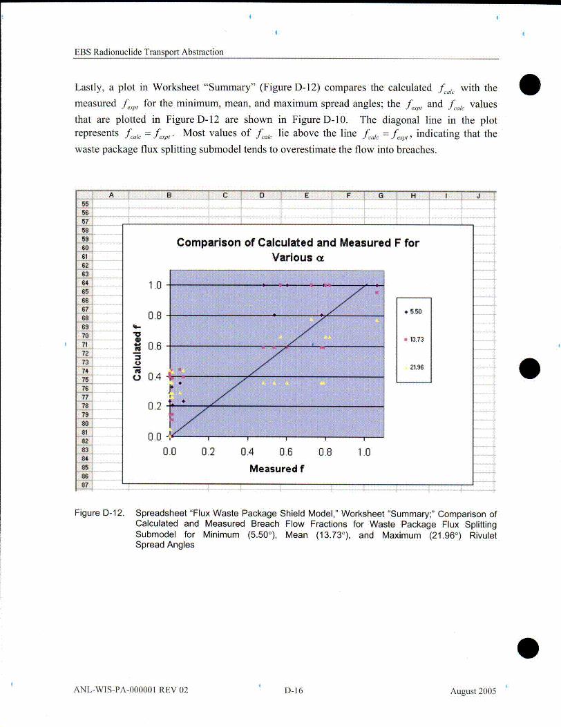
EBS Radionuclide Transport Abstraction
Lastly, a plot in Worksheet "Summary" (Figure D- 12) compares the calculated fea,, with themeasured fexp, for the minimum, mean, and maximum spread angles; the fxp, and fcaic values
that are plotted in Figure D-12 are shown in Figure D-10. The diagonal line in the plotrepresents fc1,i = fe.pt" Most values of fc.ac lie above the line f,,,,, = fexp,, indicating that the
waste package flux splitting submodel tends to overestimate the flow into breaches.
0
57585960
61
•2
83
646566676868707127273747i51
.77!
828=3
85-J86~8=7
I -- - -- -- L
Comparison of Calculated and Measured F forVarious z
1.0
0.8 .5.50
7 • 13.73~0.6
21.96
0.4
0.2
0.0
0.0 0.2 0.4 0.6 0.8 1.0
Measured f
Figure D-12. Spreadsheet "Flux Waste Package Shield Model," Worksheet "Summary;" Comparison ofCalculated and Measured Breach Flow Fractions for Waste Package Flux SplittingSubmodel for Minimum (5.500), Mean (13.73°), and Maximum (21.960) RivuletSpread Angles
SANL-WIS-PA-000001 REV 02 D-16 August 2005

EBS Radionuclide Transport Abstraction
APPENDIX E
MICROSOFT EXCEL SPREADSHEET "FLUX SPLITTING VALIDATION"
ANL-WIS-PA-000001 REV 02 August 2005

EBS Radionuclide Transport Abstraction
ANL-WIS-PA-000001 REV 02 August 2005

EBS Radionuclide Transport Abstraction
MICROSOFT EXCEL SPREADSHEET "FLUX SPLITTING VALIDATION"
SPREADSHEET "FLUX SPLITTING VALIDATION"-WORKSHEET "SPLASHRAD VS NUMBER"
A.O _ _ F B H 19 -_.! .... I 1- -7 5 7 7 = _Q- Correlation of Splash Radius and Number of Drips2
Fringe ormker (0)
5 Lekl Riqil Mo.0 011 Orke, Marrae.2 2 1o I 115 25.5 11 05 4 21 115 4265 21 0
10 185 Z2 s I725. 75.5 so 0
tZ 1 35 48 143 i _13 54 2.5 143 014 r 35 40 203 1
35 4 21 9,1? 371 5 7 21 0
Al 105 IS 82IS 03 32 82 0"0 315 30 us-2 45 40 20722 7.5 9 3D
2 I 2 F 27.5 37 I
Std Do...ln
MO0 to W -P0 20 250
NMiiber at' 0(01)
F25 23 20 1 55 I t.a For this plot organted in bottor table (,sae dta w table to the Wet, Wo ognird f• pottfing bl Inner C~ote (Q or 0 ut01 Frin. (0)
27 5 33525 3.9. . . .
Figure E-1. Spreadsheet "Flux Splitting Validation"-Worksheet "Splash Rad vs Number;" Effect ofNumber of Drips on Splash Radius
In this worksheet (Figures E- 1 to E-3), the effect of the number of drips on the splash radius isanalyzed using data from dripping on the crown in the rough drip shield tests. This analysis isused for validation of the drip shield flux splitting submodel. The splash distance or radius (cm)to the left and to the right of the drip location are listed in Columns A and B, respectively. Thenumber of drips in each test is given in Column C. The type of measurement-inner cluster (I) orouter fringe (0)-is indicated in Column D. These data and the DTN from which they wereobtained (MO0207EBSATBWP.021 [DIRS 163399]) are also presented in Table 7.1-1. InRow 26, the sum of the splash radii is shown. Rows 27, 28, and 29 give the mean, standarddeviation, and median for each column. The mean, standard deviation, and median for all 40splash radius measurements are listed in Column G, Rows 11, 12, and 13, respectively.
The plot to the right in Figure E- 1, which is reproduced as Figure 7.1-1, shows the dependence ofsplash radius on the number of drips. As indicated beneath the figure, the data are the same as inthe table, but organized by type of measurement further down in this worksheet. The Trendlinetool in Microsoft Excel is used to fit a quadratic curve to the inner cluster and outer fringe data.The correlation coefficient is shown for each curve, and the correlation equation is shown for theinner cluster curve. A second degree polynomial was chosen for the Trendline in order todisplay the expected behavior-the splash radius should increase with the number of drips, buteventually reach a maximum. A functional form such as y = Ymax(- may be moreappropriate, but because this is nonlinear in the fitting parameter a, a simple linear least squaresfit using Trendline is not possible. Since the object is simply to demonstrate a correlation, amore accurate fit to the data is not necessary.
ANL-WIS-PA-000001 REV 02 E-1 August 2005
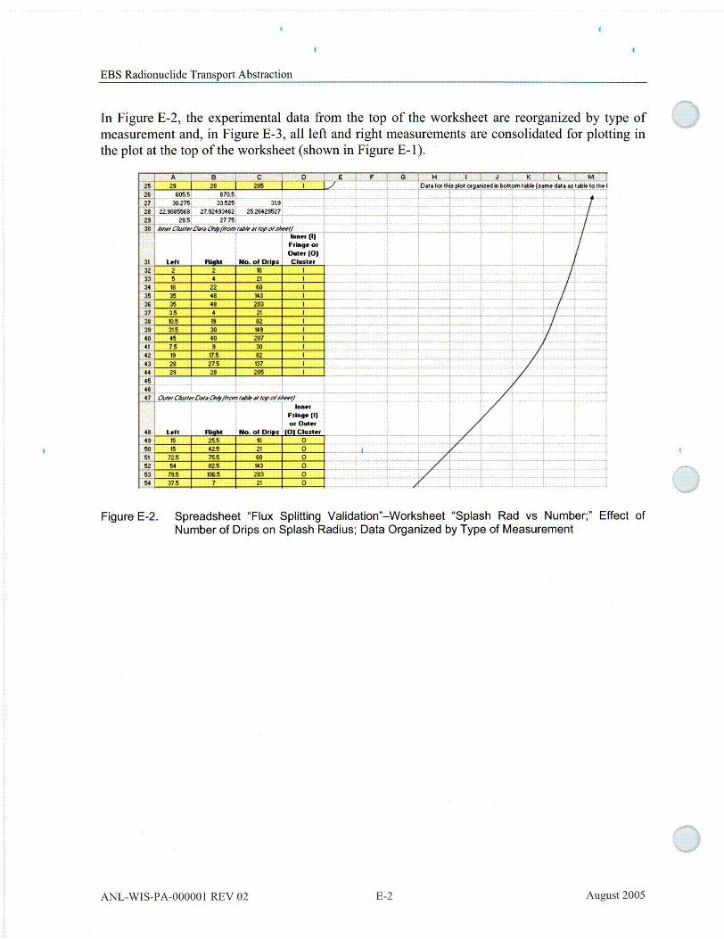
EBS Radionuclide Transport Abstraction
In Figure E-2, the experimental data from the top of the worksheet are reorganized by type ofmeasurement and, in Figure E-3, all left and right measurements are consolidated for plotting inthe plot at the top of the worksheet (shown in Figure E-1).
F IS H I I ~I K L M
_;7t
2828 28 1 Cl EA B ~ I ~ L' Ft. H9i I .P l orI , tI _ I tt t t a as_ tL o tData for Whs plo organizod in bottom table (same data as table* to the I
605.5 678.530.275 33.52 31..9
22.9085568 27.52493462 25.2642952728.5 27.75,
bler (I)FrInge orOwter (0O
tut Uo_ oat be Clbster2132 2 2 10 1___
5 4 21 14 22 so I
35 48 143 135 48 203 1
37 3.5 4 21 I
38 10.5 19 82 _____
38 3t5 30 19, 140 45 40 207 I41 7.5 9 30 142 19 ITS 82 I4A3 28 27.5 137 ____
4!4 29 28 205 _______
4548
Ji4 4FrhWg (1)ot outer
48 LMf t Mo. of Drips l0iCluster
15 25.5 t0 015 42-5 21 0
72.5 I755 so 054 V2.5 143 0
5 7&5, 106.5 203 037.5 7 21 0
Figure E-2. Spreadsheet "Flux Splitting Validation"-Worksheet "Splash Rad vs Number;" Effect ofNumber of Drips on Splash Radius; Data Organized by Type of Measurement
ANL-WIS-PA-000001 REV 02 E-2 August 2005

EBS Radionuclide Transport Abstraction
A B 1 LI54A?5.5560SI62 R#~vd#f~d/JdAv#4b ?(dM.'bC.71(d.4. M&'~%WI
F I- Q H 1 1 J K L M
64 h14r CkteI Outet Fn'e658 of O'lr Radiu cm 8 of Icips Radius cm
10 2 10 1521 5 21 15
68 6o 18 60 72,6 143 35 143 5470 203 35 203 78.5
21 3-5 21 37.572 82 10.5 82 6373 148 31.5 t0 25.574 207 45 21 42.575 30 7.5 6O 75.576 82 19 143 82.577 137 20 203 M08.578 205 28 21 771 -10 2 82 3280 2181 60
82 143203
84 2185 82
6 14920730
8 8291 20
92
42248484
30409
171527.529
Figure E-3. Spreadsheet "Flux Splitting Validation"-Worksheet "Splash Rad vs Number;" Effect ofNumber of Drips on Splash Radius; All Left and Right Measurements Are Consolidated
SPREADSHEET "FLUX SPLITTING VALIDATION"-WORKSHEET "SPLASHRADIUS"
For validation of the drip shield and waste package flux splitting submodels, splash radius dataare analyzed for measurements on the rough drip shield surface, with dripping on the crown andat off-crown locations. Data for crown drip locations are used for the drip shield submodelvalidation, and off-crown drip locations are used for the waste package submodel validation.The statistics (mean, standard deviation, median, mean plus one standard deviation, and meanminus one standard deviation) are shown in Column I, Rows 19-23 for crown drip locations, andin Rows 37-41 for off-crown locations. The data actually used in the model validation are theminimum and maximum values for more than 20 drips, Cells H 11 and 19, respectively, for crownlocations, and Cells H31 and 136, respectively, for off-crown locations.
ANL-WIS-PA-000001 REV 02 E-3 August 2005

EBS Radionuclide Transport Abstraction
2 Splash Radius Determination, Rough Drip Shield Surface, Dripping on Crown23 Sour@* Dma
5 S Srae.s Left ) Rght cm)_ Splash Radius Test 61- Rough DS Surface- Ctown
so 1&.0 22.0143 35.0 48.0
10 1203 35.0 48.01I Splash Radius Test 62- Rough DS Surface- Crown 21 3. 4.0
82 10.5 18.01 149 31.5 30.0
14 207 45.0 40.0SSplash Radius Test 63io- Rough DS SurfaceS- Crown 30 7.5 9.0
1682 1t.0 17517 137 28.0 27.5
16205 29.0. 28.019 Meana
2=01 Std. 0v.21 Meda22 Mean-SO23 Mean.SO2425
28 Splash Radius Determination, Rough Drip Shield Surface, Dripping off Crown27
Somse* Data
30 #Onip Left (cm) Rih en31 Splash Radius Test #4- Rough DS Surface -33 degrees Ij 1 3i5 .5
_33 M5. OTN: MIO207EBSATBVI
N
P.021
-34 Splash Radius Test #5 -Rough DS Surface -16.5 degrees 22 9 035 82 13 14J3s- 15N 141 L537 Mean
39 Median40Mean-SD4_1 Mean.SD
14 WN43 dvF~x*e lash Rais~N~~j~1fS9fWýPrpadB '-41
DTN: MO0207EBSATBWP.021 [DIRS 163399].
Figure E-4. Spreadsheet "Flux Splitting Validation"-Worksheet "Splash Radius;"Determination
Splash Radius
ANL-WIS-PA-000001 REV 02 E-4 August 2005

EBS Radionuclide Transport Abstraction
SPREADSHEET "FLUX SPLITTING VALIDATION"-WORKSHEET "ROUGH DS"
This worksheet provides calculations for validation of the drip shield flux splitting submodelbased on data from rough drip shield surface tests. An overall view of the worksheet is shown inFigure E-5 to show the layout of the worksheet, and individual tables are then presented morelegibly and described in detail on following pages.
s.. . 1 1t; ;.. 1...I 81. "41.41;. *r...5 If .00..
.53ks
I.I'14
14I,
II * .1a
* ,.Ie 3 I;a C 1. * IhU~ SS
- I ElE 01
St --
4t U..ka&*I2 Q IQI
LII
54.0....11.4;.. -
4~a,
41
-wii
aII'V-Ii
I'II
11
Ii'I41aft
a
-w'I
4 4
OEMIV2mc~
tllll
Cilf\T S! E.2;WE
P HNq3tadh AMs Nurmber _ýRqugh ~~9fconw o ]1A
DTN: MO0208EBSATBWP.027 [DIRS 163404]; DTN: MO0208EBSATBWP.028 [DIRS 163405].
Figure E-5. Spreadsheet "Flux Splitting Validation"-Worksheet "Rough DS;" Worksheet Overview
ANL-WIS-PA-000001 REV 02 E-5 August 2005

EBS Radionuclide Transport Abstraction
A B C 1 .... E F.1 Drip Shield Model Valication Using Rough Surface Data, On-Crown Results
G H
23-j Source Data4]
6 InputTare Input Final Input (g)7 M,#•to P~h-h Tp.qIq oTh~,nh fl5 •u~rpfl114DT: MOO208BEASATBWPJ127
B4 Initial 84 Final B4 Inflow f4p (84)
8 81 cm left of DS center 2947 26288 292.351 106.461 106.731 09 i24 cm left of DS center 1 68.451 -220.001 288.451 106.41 1.19 106.6
10 27 cm right of DS center 1 6819 -223.43 29.61 0.001 0,001 0.11 27 cm right of DS center 1 41.521 -252.61 294.1316.601 0.001 0012 81 cm right of DS center 1 78711 -211.391 290.10 00 00 0.013 Sounding Flow Rate Tests, Rough DS Surface DTN: MOO208EBSATBWP.02814 54 cm left of DS center tHigh) 813.08 482.34 330.74 107.43 301.30 193.815 27 cm left of DS center (High) 788,15 459.50 328.65 99.75 100.38 0.611§ 27 cm right of DS center (High) J 74425 43760 306.65 0.00 0.00 00ý17 27 cm right of DS center (Low) 874.55 329.41 54514 0.0 0.00 00.18 27lcmright ofDS center (Low) J 74.80 674.00 70.80 0.00j 0.019 27 cm left of DS center (Low) 815.25 701.93 11332 107.50 106.86 1.320 54 cm left of DS center (Low) 695.48 577,38 118,10 0.00, 0.00 0.0
23
Breaches that sho
DTN: MO0208EBSATBWP.027 [DIRS 163404]; DTN: MO0208EBSATBWP.028 [DIRS 163405].
Figure E-6. Spreadsheet "Flux Splitting Validation"-Worksheet "Rough DS;" Calculation of ExperimentalBreach Flow Fractions
", ' ' _ , ., . , ' '.' = • . . • .. I U t .' '-
23
H ~ I. ~' 4 K I -It N 0- I.. ~
456 / . (B4) B5 Initial B5 Final B5 Inflow
14 0.00 0.00 0.00
__ 0.00 0.00 0.00
10 109.60 109.73 0.3919 0.00 0.00 0.0020 0.00 0.00 0.00
21Breaches that should have flow are highlighted in bold.23
i(B5)
leantd. 0ev.ledian
Figure E-7. Spreadsheet "Flux Splitting Validation"-Worksheet "Rough DS;" Summary of ExperimentalBreach Flow Fractions
ANL-WIS-PA-000001 REV 02 E-6 August 2005

EBS Radionuclide Transport Abstraction
Tests are identified in Figure E-6 in Column A. Columns B and C are raw data-the initial andfinal water mass in the input water container. Column D is the difference between Columns Band C (e.g., D8=B8-C8), giving the mass of water dripped onto the drip shield. Columns E andF are the initial and final masses of water in the Breach B4 collection vessel. The difference, inColumn G (e.g., G8=F8-E8), is the mass of water that flowed into B4. In Column H(Figure E-7), the fraction of the dripping flux that flowed into B4, fexp, (B4), is calculated fortests in which the flow into B4 was greater than zero (e.g., H8=2*G8/D8). Because the drippingwas onto the crown, it is assumed that only half of the total input (i.e., D8/2) flowed down theside of the drip shield where B4 was located.
Columns I and J are the initial and final masses of water in the Breach B5 collection vessel. Thedifference, in Column G (e.g., K8=J8-18), is the mass of water that flowed into B5. InColumn N, the fraction of the dripping flux that flowed into B5, fewp, (B5), is calculated for testsin which the flow into B5 was greater than zero (e.g., NI0=2*K]0/D]0). Because the driplocation was the crown, it is assumed that only half of the total input (i.e., D] 0/2) flowed downthe side of the drip shield where B5 was located.
The input water mass and flows into Breaches B4 and B5 are summarized in Table 7.1-3.
In Column P, all values of LIP, are consolidated. The mean, standard deviation, and median forthe 12 data values are given in Rows 21, 22, and 23, respectively. The values of fexp, are listedin Table 7.1-4.
25 RhvuWe Spiead Distan"26 _______________cd Me Ewemrtmnl(c
27 BTU: MMMO8ESATOVP027 - OM LO - R*
__ __ __ __ __ __ _4_ 136-00 32 9.520 N7IVIR.nM. 4 13.00 M15 ___
3127*md*A1SO**.i 5 86.00 0 ____
32 8Iof kMdOS emanl- 6 86.0 1 34&4vnSWFkoWRM, rPSt ROVOLK.$Wg"
33QTH M 640020SESATBVP.02 ___
34 f 54m.of DS MtmlI4ffi, 4. MOOhhi~EIII 2 035 '27 OM " f S0~0ScctecI4 4 136.0 15 1
3627 emrigM oEDS c~P4~1% 5 96.00 6..... 637 27 wn 6*4of S ooi Low1 5 KOO.A 50 ____
30 27 OMNM f Slet(ow) 5 KOO 1M9:27 mornkto S emor ILowl 4 MOO 2&5
40 54 cm" f S cu~ (Low) 4 Moo0 0 0
I spcead "SitIe
I .... I .. I IAv.;ag.25,0019.n•
10.0c0.50
2550i
0.00 KO6
Mean=Std Den..
Medan .104D
Madmum.Mewiffn.-
41742
450
I AN rpe:ad Din I pfad ar :e
DTN: MO0208EBSATBWP.027 [DIRS 163404]; DTN: MO0208EBSATBWP.028 [DIRS 163405].
Figure E-8. Spreadsheet "Flux Splitting Validation"-Worksheet "Rough DS;" Rivulet Spread Distances
Rivulet spread distances for each test are listed in Figure E-8, Columns D and E, Rows 28-40, fordrips originating on the crown of the rough drip shield surface. The spread data are reorganizedin Column B, starting in Row 52 (see Figure E-9). All spread data measured 86 cm from the drip
ANL-WIS-PA-000001 REV 02 E-7 August 2005

EBS Radionuclide Transport Abstraction
location are listed first, followed by all data measured 136 cm from the drip location. Thecorresponding x-distance is listed in Column C, starting in Row 52. In Column E, the spreaddistances, wr, are converted to spread angles using the formula:
a = tan-l(1-j.
In Cell E52, for example, the Microsoft Excel equation is: E52=ATAN(B52/C52). The resultis the spread angle in radians, which is converted to degrees in Column F(e.g., F52=DEGREES(E52)). The mean spread angle for 86-cm drips is given in Cell 155(155=AVERAGE(F52:F63)) and for 136-cm drips in Cell 169 (169=AVERAGE(F65:F75)).Statistics are computed for all individual spread angle data in Column F, Rows 77-82:
F77=AVERAGE(F52:F75)
F78=STDEVA(F52:F75)
F79=F77-F78
F80=F77+F78
F81=MIN(F52:F75)
F82=MAX(F52:F75)
As shown in F79 and F80, the range for the spread angle is zero (rounding down) to 14.40.
&9.ý05
AN aD.1.
17.0 OW.0
A00 NM.0too0 0".0
XOD0 0"0&00 00
3250 00600I 1W
a - 15.0 t
2&50.0 900.00AW-
7 7.50 MOO
72 9100 MW0
74 V5.00 moo76750.001 1060
70
7906
829364
4 4 ~ ~ /S~ash~, _S Rough DSZ Rt-fawn~mt /
Figure E-9. Spreadsheet "Flux Splitting Validation"-Worksheet "Rough DS;" Rivulet SpreadData Reorganized
ANL-WIS-PA-000001 REV 02 E-8 August 2005

EBS Radionuclide Transport Abstraction
pirip Shield ModelSpread anal& F=113.5 1.tamadill Drop Shield Model
EBS Radionuclide Transport AbstractionI
A- I
I I I I IAverag 2 (am]
25.00 138O19.75 1MA.10.0 8600.50 NOC
2M. -d
1.00 IS015.00 .016.00 - W
33.00 88.011.00 88.01
18.7 3600.001 138.0
Mean.Std. Dev.:MedianMean -1 IStd. Dey.Mean -1 Std. 0ev.MaXimum:minimum:
I I I
tLength from cronto rivulet Xmeasurement 1/ 2 Spread angle
112 spread(measured in Total Spread= 2xtan6experiments)
wNSls ad ývsNWY6&ber Sp RoL41D4-Lf-off Co~pwn -WP model-
Figure E-1 0. Spreadsheet "Flux Splitting Validation"-Worksheet "Rough DS;" Calculation of RivuletSpread Angles
In Column H, Rows 28-40 (see Figure E-10), the average rivulet spread is computed for eachexperiment (e.g., H28=(D28+E28)/2). Column I is the distance from the crown to the pointwhere the rivulet spread was measured (identical to Column C). The spread angle is computedin Column J, Rows 28-40, (e.g., J28=ATAN(H28/128)). In Column K, Rows 28-40, the
ANL-WIS-PA-000001 REV 02 E-9 August 2005

EBS Radionuclide Transport Abstraction
average spread angle in radians is converted to degrees (e.g., K28=DEGREES(J28)). InWorksheet "Splash Rad vs Number," the minimum splash radius for tests using 20 or more dripswas 3.5 cm, for a total splash distance of 7 cm. This is used as the effective drip shield length inColumn L, where fcac is obtained using the formula
f ti =({1 tana~
-13.5( tan a)
L28=1 3.5*(1 +TAN(J28)/2)/7
The maximum splash radius tests using 20 or more drips was 48 cm in Worksheet "Splash Radvs. Number," giving a total splash distance of 96 cm. This is used as the effective drip shieldlength in Column M:
=13.5 (C tana'\
M28=13.5*(1 +TAN(J28)/2)/96
The values of fcaic in Columns L and M are similar to F/fIvD in Table 7.1-5, the only differencebeing the values used for spread angle. Table 7.1-5 uses the rounded values for spread angleobtained from Figure E-9, zero to 14.4', whereas in Columns L and M in Figure E-10, faic is
calculated from a different average spread angle.. As shown in the statistics (Rows 46-47), fc•1 c
or F/fvA ranges from 0.141 to 2.30, based on minimum and maximum average spread angles.
Using the mean plus or minus one standard deviation for the spread angle, fc,1c rangesfrom 0.141 to 2.16 (Rows 44-45, Columns L and M), close to the values reported in Table 7.1-5(0.141 to 2.17).
In Column N, Rows 28-40, the values of f.p, are transferred from Column P, Rows 9-20. In
Column 0, the ratio f,ýpt, /fco is computed (e.g., 028=N28/L28) for the minimum effective
drip shield length of 7 cm. In Column P, the ratio f,,,, lfc/fc is computed (e.g., P28=N28/M28)
for the maximum effective drip shield length of 96 cm. This ratio is identical to the uncertaintyfactor fvD in Equation 7.1.1.1-2. As shown in the statistics (Rows 46-47), F/lfv for theexperimental data ranges from 0.0 to 8.306
ANL-WIS-PA-00000I REV 02 E-10 August 2005

EBS Radionuclide Transport Abstraction
SPREADSHEET "FLUX SPLITTING VALIDATION"-WORKSHEET "ROUGH OFFCROWN WP MODEL"
This worksheet provides calculations for validation of the waste package flux splitting submodelbased on data from the rough drip shield surface tests. An overall view of the worksheet isshown in Figure E-11, and individual tables are then described in detail.
MEOW=. .
a. ,lf ...a.MWb-9 fS .. ,..V,: ......
14 41 mN,-VaO s ~JterL haus~~D )~ougff crown WPjM4 f4e! I J --
Figure E-1 1. Spreadsheet "Flux Splitting Validation"-Worksheet "Rough off crown WP model;"Worksheet Overview
0ANL-WIS-PA-000001 REV 02 E-11I August 2005
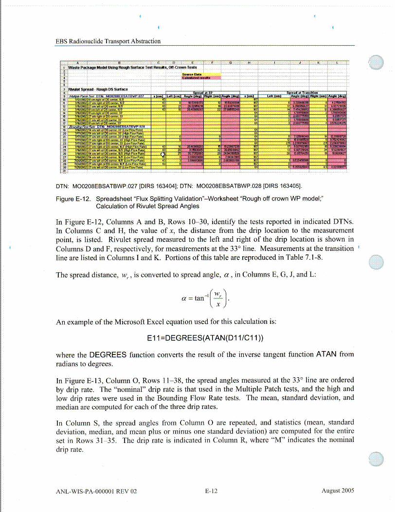
BBS Radionuclide Transport Abstraction
I -t K I.__B _ ff __5 _ i .. .g_ K ].. [ Ii. N j
Waste Packag Model Using Rough Surfac Test Resulte, Off-Crown Tests
3 Soawe Data-.A-
5
7 ORMetSpread -RoughlOS Surface _________________Ifi s.a4t 33 r
*&tPeAeq0N P40208SS TSW27 2L
h
127 WAofS ww, 33*
16 766400 2 o f E~DSoor.O 33'
2l8 0 o.I:to rouvatEUSAO - __
711 6 0 0f4.d' i
__ wM17 WO 432? 71020 Mwo.~d~~B 165 P oFo. *e U__ I
01 w 6¶.5HOFdOý Ml 4.'__
64764,
--- 164
64
Left Io~
DTN: MO0208EBSATBWP.027 [DIRS 163404]; DTN: MO0208EBSATBWP.028 [DIRS 163405].
Figure E-12. Spreadsheet "Flux Splitting Validation"-Worksheet "Rough off crown WP model;"Calculation of Rivulet Spread Angles
In Figure E-12, Columns A and B, Rows 10-30, identify the tests reported in indicated DTNs.In Columns C and H, the value of x, the distance from the drip location to the measurementpoint, is listed. Rivulet spread measured to the left and right of the drip location is shown inColumns D and F, respectively, for meastrements at the 330 line. Measurements at the transitionline are listed in Columns I and K. Portions of this table are reproduced in Table 7.1-8.
The spread distance, wr, is converted to spread angle, a, in Columns E, G, J, and L:
a = tan-i-).
An example of the Microsoft Excel equation used for this calculation is:
El1 =DEGREES(ATAN(D1 1/C011))
where the DEGREES function converts the result of the inverse tangent function ATAN fromradians to degrees.
In Figure E-13, Column 0, Rows 11-38, the spread angles measured at the 33' line are orderedby drip rate. The "nominal" drip rate is that used in the Multiple Patch tests, and the high andlow drip rates were used in the Bounding Flow Rate tests. The mean, standard deviation, andmedian are computed for each of the three drip rates.
In Column S, the spread angles from Column 0 are repeated, and statistics (mean, standarddeviation, median, and mean plus or minus one standard deviation) are computed for the entireset in Rows 31-35. The drip rate is indicated in Column R, where "M" indicates the nominaldrip rate.
ANL-WIS-PA-000001 REV 02 E-12 August 2005

0EBS Radionuclide Transport Abstraction
In Column U, the spread angles from Columns J and L are consolidated for measurements at thetransition line. The drip rate used in each test is indicated in Column T. (The values in thiscolumn are currently incorrect, since they are just copies of the incorrect results in Column L andincorrectly recalculated values from Column J, where the actual Column J values are correct.)
All 50 spread angle measurements are compiled in Column W, with statistics (mean, standarddeviation, median, and mean plus or minus one standard deviation) computed for the entire set inRows 63-67 (Figure E-14). The mean plus or minus one standard deviation are used as thespread angle range in Section 7.1.1.2 for determination of the uncertainty in the waste packageflux splitting submodel validation.
I P ! , "-,N R I S TU j V
23-
41
14
14
18t1-
N2227
28
32:
38
41
42
48 1,, (B5
Slpad AnglesOrderd bg Dripl Rate
Rtsge
Mean
M•eda~n
Mean
St.0ev -
mean
Std 0evMedan
A!l
Spash Ra sNubrR~alu
Sp,.ad AngletsDidered bg istance
haom Drip
J Rusqgh off crown WP model/ 1I4J
Figure E-13. Spreadsheet "Flux Splitting Validation"-Worksheet "Rough off crown WP model;" AdditionalCalculations of Rivulet Spread Angles
ANL-WIS-PA-000001 REV 02 E-13 August 2005

EBS Radionuclide Transport Abstraction
Me-Std Dey.Meian~O~
MeanStd. Dev.
mean I Std. Dev.'Mean *I Std. bey.
Figure E-14. Spreadsheet "Flux Splitting Validation"-Worksheet "Rough off crown WP model;" Statisticsof Rivulet Spread Angles
48ho_____ ut Tan F" Imt [s 14 ImkitaI B4 FinalI B4kifow I IB4141 71 DTWi. W09I0SE13SAYWRP027
51 __7l152 127 cm to ~~t,15824.2 507.4800
56 2002127 cmeWt of DScenw, 3x
-67 __ of E15 cactw. JT 68i223 551182 059 ~ ~ ~ 1Yd 4WUBAR#.Z
- W0 54 an7 Wto S om 3 k7 ~)W-3 AI2021 94
|-- L
637i r 7i fD " fLOW"7
5bW .
BrEachesthatshod h.ae lwaehhltedibl.
71
DTN: MO0208EBSATBWP.027 [DIRS 163404]; DTN: MO0208EBSATBWP.028 [DIRS 163405].
Figure E-15. Spreadsheet "Flux Splitting Validation"-Worksheet "Rough off crown WP model;"Calculation of Experimental Breach Flow Fractions
For the tests identified in Columns A and B, Rows 50-70 (Figure E-15), the initial and finalwater mass in the input water container are listed in Columns C and D, and the amount of waterdripped onto the drip shield is calculated in Column E (e.g., E50=C50-D50). The initial andfinal mass of water in the Breach B4 collection vessel is listed in Columns F and G, respectively,and the amount of water collected from flow into Breach B4 is calculated in Column H(e.g., H52=G52-F52). The fraction of water dripped onto the drip shield that flowed intoBreach B4, f,ýrp, (B4), is computed in Column I for the tests in which the inflow was greater than
zero (e.g., 152=H52/E52).
ANL-WIS-PA-000001 REV 02 E- 14 August 2005

EBS Radionuclide Transport Abstraction
Figure E-16. Spreadsheet "Flux Splitting Validation"-Worksheet "Rough Off Crown WP Model;"Summary of Experimental Breach Flow Fractions
The initial and final mass of water in the Breach B5 collection vessel is listed in Figure E-16,Columns I and J, respectively, and the amount of water collected from flow into Breach B5 iscalculated in Column L (e.g., L50=K50-J50). The fraction of water dripped onto the drip shieldthat flowed into Breach B5, fe,, (B5), is computed in Column M for the tests in which theinflow was greater than zero (e.g., M50=L50/E50).
The 20 values of LIP, are compiled in Column P, with statistics (mean, standard deviation,median, and mean plus or minus one standard deviation) presented in Rows 73-76.
The input water, breach inflows, and f,,p, for each breach are reproduced in Table 7.1-10.
ANL-WIS-PA-000001 REV 02 E-15 August 2005

EBS Radionuclide Transport Abstraction
INTENTIONALLY LEFT BLANK
ANL-WIS-PA-000001 REV 02 E-16 August 2005

EBS Radionuclide Transport Abstraction
APPENDIX F
MICROSOFT EXCEL SPREADSHEETS "TRANSPORTCALCALLCOLLOIDS,""FLUXOUTRATIO.XLS," AND "TIMETOCONV.XLS"
ANL-WIS-PA-000001 REV 02 August 2005

EBS Radionuclide Transport Abstractioh
ANL-WIS-PA-000001 REV 02 August 2005

EBS Radionuclide Transport Abstraction
MICROSOFT EXCEL SPREADSHEETS "TRANSPORTCALCALLCOLLOIDS,""FLUXOUTRATIO.XLS," AND "TIMETOCONV.XLS"
SPREADSHEET "TRANSPORT CALC ALL COLLOIDS.XLS"
The purpose of this spreadsheet is to implement the colloid model that represents the sorption ofradionuclides onto the oxy-hydroxide (designated FeO) corrosion material within the engineeredbarrier system (EBS). The model accounts for both reversible and irreversible sorption onto theFeO mobile colloids and the immobile corrosion products together with reversible sorption ontoboth waste form and groundwater (GW) colloids. This description refers to equations inAppendix B, "Implementation of Radionuclide Sorption onto Colloidal and Stationary Phaseswith Finite Difference Solution."
Description of Input Values
The first 29 rows of the worksheet (see Figure F-I for an image of the worksheet) containparameter input values. Column D contains the typical values input from the GoldSimmodel. Column B contains values from Column D that are scaled appropriately for thecurrent calculations.
Row 2: cs [kg/mA3],
c, = Pu solubility
$B$2=$D$2/1000
Row 3: phi_1
_ celll , 0 - pOre , porosity of the upstream boundaryVbulk
$B$3=$D$3
Row 4: phi_2
V_cell2, = pore, porosity of the corrosion product mass
Vbutt
$B$4=$D$4
Row 5: phi_3
V0 ce113, 0 = pore, porosity of the downstream boundary
Vbulk
$B$5=$D$5
Row 6: U [mA3/yr]
volumetric water flux, U Table B- 1
ANL-WIS-PA-000001 REV 02 F-1 August 2005

EBS Radionuclide Transport Abstraction
$B$6=$D$6
Row 7: KdFeO_c [mA3/kg]
partition coefficient in the FeO colloid state
$B$7=$D$7/1 000
Row.8: KdFeO_CP [mA3/kg]
partition coefficient in the stationary FeO corrosion product state
$B$8=$D$811 000
Row 9: Kd_WFc [mA3/kg]
partition coefficient in the waste form colloid state
$B$9=$D$9/1000
A I B C I D1 Input for Excel sreadsheet Input from GoldSim2 cs[kg/mA3] 0.001 cqs[mg/LJ 13 phi-1 1 phi 1 14 phi 2. 0.4 phi.2 0.45 phi_3 0.3 phi3 0.3Su[rn3/yr] 0.1 u[m^3/ yr 0.1
7 Kd FeO c [mA3/kg]_ 1.000OOE+01 KdFeOqc[mI/g] 1.OOOOOE+048 Kd FeOCP_[mn3/kg] 2.50000E+00 Kd FeO CP [ml/g1 2.50000E+039 Kd WF c [mA3/kg] 2.00000E+02 KdWF c [ml/_g 2.OOOOOE-i0510 Kd GW c[mA3/kg] 2.00000E+02 Kd GW c [mI/g] 2.00000E+0511 mass FeO CP Ik g]I 1.80000E+04 mass FeO CP[g] I 1.80000E-0712 Y_.re [m3]_ 2.29008E+l0 V pore [U____ 2.29008E+0313 c FeO q [kg/mA3] I 2.OOOOOE-021c FeO qc[mg/1_] j 2.OOOOOE+01!14 c FeOCP [kg/mA3_ I 7.86000E-403 c FeO CP lmng/L] 7.86000E406-15 c WF c [kgfmA3. 3.OOOOOE-03 c WF cmg/L] 3.00000E+0016 c GW c [kg/mA3] 1.00000E-04 c GW c [mgq 1.000OOE-0117 rate [myd 1.OOOOOE-05 rate [cm/ynr- 1.00000E-03
U;
18 S FeO JmA2/kg]_ 1.00000E*051S FeO [m!2/ 1.00.OOOOOE+0219 S FeO CP_[nA2/kg] 1.00000E+041S FeO CP [mA2/g] 1.OOOOOE+0120 d FeO lkq/mA3l 5.24000E+03 den FeO [kq/mA3| 5.24000E+0321 diffus aqJmA2/yr] 7.25834E.02 diffus !!q lmA2/s] 2.30000E-0922 diffus colloid [mnA2/yrj 7.25834E-04'diffus colloid [mA2/ 2.30000E-1123 diff length_ [19] 1.OOOOOE-03 diff length. 1[m] 1.00000E-0324 diff length 2[rn] 5.00000E-00 n difflegnLh_.2_[m__ 5.OOOOOE+00251diff length 3_[n] 8.06000E-01 diff length_ _[m] 8.06000E-0126 duiff area 1 2 [mA2] 3.60000E+01 diff area 1_2[m^21 3.60000E+0127 1diff area 2 3 [mA2J 1.06800E-00 diff area 2 3 [mA2] 1.06800E+00281 decay [l/yr] 2.87494E-05 decay [l/yr] 2.87494E-0529 delt [yd 10 deltly[A 10
Figure F-1. Spreadsheet "TransportCalc all colloids.xls;" Summary of Inputs K);
ANL-WIS-PA-000001 REV 02 F-2 August 2005

EBS Radionuclide Transport Abstraction
Row 10: KdGW-c [m^3/kg]
partition coefficient in the GW colloid state
$B$1 0=$D$1 0/1000
Row 11: massFeOCP [kg]
m1 FeO-CP = mass of corrosion product
$B$1 1=$D$1 1/11000
Row 12: Vpore [mA3]
Vpore = OVh.l,- =-O-cP , pore volume0 - b PFeO_CP
$B$12=$D$12/1000
Row 13: cFeO.c [kg/mA3]
CPUFeO_c, concentration of Pu in the FeO colloid state from reversible sorption
$B$13=$D$13/1000
Row 14: cFeOCP [kg/mA3]
cpur FeO cp , concentration of Pu in the stationary FeO corrosion product state from
reversible sorption
$B$14=$D$14/1000
Row 15: cWF-c [kg/mA3]
cPu-C'F , concentration of Pu in the waste form colloid state from reversible sorption
$B$15=$D$15/1000
Row 16: cGW-c [kg/mA3]
Cp.- Gil' , concentration of Pu in the GW colloid state from reversible sorption
$B$16=$D$16/1000
Row 17: rate [m/yr]
k, forward rate constant (M 3 water m-2 FeO yr-')
$B$17=$D$17/100
ANL-WIS-PA-000001 REV 02 F-3 August 2005

EBS Radionuclide Transport Abstraction
Row 18: SFeO_c [mA2/kg]
SFeO = specific surface area of FeO (in 2 kg-') in the colloid state
$B$18=$D$18*1000
Row 19: SFeOCP [mA2/kg]
SFeO = specific surface area of FeO (m2 kg-') in the corrosion product state
$B$19=$D$19*1000
Row 20: dFeO [kg/mA3]
PFýocp = corrosion product (FeO) density (kg m73)
$B$20=$D$20
Row 21: diffus-aq [mA2/yr]
Daq = aqueous diffusivity (M 2 yr-)
$B$21 =$D$21 *31558000
Row 22: diffuscolloid [mA2/yr]
DcIoid = colloid diffusivity (mi2 yr-')
$B$22=$D$22*31558000
Row 23: diff length1 [m]
L, = diffusive length for cell_1
$B$23=$D$23
Row 24: diff length_2 [m]
L2 = diffusive length for cell_2
$B$24=$D$24
Row 25: diffjlength_3 [m]
L3 = diffusive length for cell_3
$B$25=$D$25
Row 26: diffarea_1_2 [mA2]
A.,2 = diffusive area at cell_] and cell_2 interface
$B$26=$D$26
ANL-WIS-PA-000001 REV 02 F-4 August 2005

I
EBS Radionuclide Transport Abstraction
Row 27: diffarea_2_3 [mA2]
A' 23 = diffusive area at cell_2 and cell_3 interface
$B$27=$D$27
Row 28: decay [l/yr]
2, decay rate (yr-)
$B$28=$D$28
Row 29: delt [yr]
At, time step length
$B$29=$D$29
Rows 30 through 53 contain additional derived parameters for the mixing cell colloid model.
A I B 6C D E F G30 R bar 1 [_/yrl_ 2.000OOE-02 _
31 Rbar 2 [1/yr) 7.86000E+t0232 U bar [1/yr] 4.36667E-02 _
33 Kd bar FeO c 2.OO000E-0134 Kd bar FeO CP 1.96500E-t04 A__35 Kd bar WF c 6.00(X0E-01 _ _
36 Kd-bar GW c I 2.00000E-021 _ _
37 K bar 1 I 1.96518E4 _ I __ _ _
38 K bar 2 1.82000E4+O) _ I39 K bar 3 8.20000E-01 _ I40 Diff leftaq 9.12736E-02 1 !41 Diff left c 9.12736E-04 ___42 Duiff_nght aq 2.22893E-03 limiting values _
43 Diff right colloid 2.22893E-05 p1 3.58485E-02 _
44 denom a 1 2 2.75194E+04 p2 8 8.17743E-02 tolerence = L 1.OOJX0E-02i45 a 1 7.14108E-01 lim c Pu aq 2.05511E-07 Pu eq time [yI]i 137
46 a 2 5.87541E-08 lim c irr c 9.40175E-08 delta 1 3.2004E-04471 b 1 6.95808E-01 lim c rev c : 4.11023E-08 delta 2 3.0078E-0448 lb 2 1.39162E-01 lim c irr CP I 5.61862E4,0 t 1 2249 e 1 9.99713E-01 lim c rev CP 1 4.03830E-03 t 2 2450 e 2 7.85774E403 flux out ratio 5.48749E-01 irry Pu c time [yrJ 24051 Omega 9.5000E-01 flux out/flux in 1.29289E-04 _
52 k.fitOmega_[cn'yr]_ 4.1837E-02 irrv coVrev col 5.57903E-01 _
53 p1/p2 4.3838E-01 F54,55
Figure F-2. Spreadsheet "TransporL.Calc all colloids.xls;" Additional Derived Parameters
Row 30: Rbarnl [l/yr]
Rl = SFeOcCFeO ck, reaction rate for colloids
$B$30=$B$18*$B$13*$B$17
ANL-WIS-PA-000001 REV 02 F-5 August 2005

EBS Radionuclide Transport Abstraction
Row 31: R-bar_2 [l/yr]
R2 = SFeOCPCFeOCPkk, reaction rate constants for corrosion products
$B$31 =$B$19*$B$14*$B$17
Row 32: Ubar [l/yr]
U is the advective rate constant
$B$32=$B$6/$B$12
Row 33: Kd barFeO c
advective dimensionless partition coefficient in the FeO colloid state
$B$33=$B$13*$B$7
Row 34: KdbarFeOCP
advective dimensionless partition coefficient in the FeO corrosion product state
$B$34=$B$14*$B$8
Row 35: Kd barWF c
advective dimensionless partition coefficient in the waste form colloid state
$B$35=$B$15*$B$9
Row 36: KdbarGWc
advective dimensionless partition coefficient in the GW colloid state
$B$36=$B$16*$B$1 0
Row 37: K bar 1
K, =I+K'--d o c + K'-_eO_CP +d + K'd cc,' ,, combination of dimensionless
partition coefficients
$B$37=1+$B$33+$B$34+$B$35+$B$36
Row 38: K bar_2
K 2 =I+Kd FeOc + KdIT c + Kd-G;wc, combination of dimensionless partition
coefficients
$B$38=1+$B$33+$B$35+$B$36
ANL-WIS-PA-000001 REV 02 F-6 August 2005

EBS Radionuclide Transport Abstraction
Row 39: K bar_3
K 3 = Kd-FeOc + Kd- Tc + Kd--G' ,, combination of dimensionless partition
coefficients
$B$39=$B$33+$B$35+$B$36
Row 40: Diff.leftaq
aqueous diffusive rate constant for left diffusive boundary condition
$B$40=($B$26/($B$23/($B$3*$B$21)+$B$24/($B$4*$B$21 )))/$B$12
Row41: Diff left c
colloid diffusive rate constant for left diffusive boundary condition
$B$41 =($B$26/($B$23/($B$3*$B$22)+$B$24/($B$4*$B$22)))/$B$12
Row 42: Diff.rightaq
aqueous diffusive rate constant for right diffusive boundary condition
$B$42=($B$27/($B$24/($B$4*$B$21 )+$B$25/($B$5*$B$21 )))/$B$12
Row 43: Diff right-colloid
colloid diffusive rate constant for right diffusive boundary condition
$B$43=($B$27/($B$24/($B$4*$B$22)+$B$25/($B$5*$B$22)))/$B$12
Row 44: denomra_1_2
denominator of a, in Equation B-55 (see Row 45)
$B$44=$B$37+($B$32*$B$38+$B$40+$B$41 *$B$35+$B$42+$B$43*$B$39+$B$30+$B$31+$B$28*$B$37)*$B$29
Row45: a_1
first order linear constant coefficient for Equation B-55,
K• +(UK 2 +D-ejq +ef_ olK---J rightaq right _cotg 3 +J- + R2 + 2K2 )AI
B$45=$B$37/$B$44
Row 46: a_2
first order linear constant coefficient for Equation B-55,(U(1+ Kd_.F c ) + Oleftq ,+- Oleft_col"Kd_ IIFc )Atcs
a2 = KI + (UK2 + DI aq + Df_~ole IkdUT c +Dright aq +Drigi,,_do1K3 + R, + R2 +2K1 At
$B$46=(($B$32*(1+$B$35)+$B$40+$B$41 *$B$35)*$B$29*$B$2)/$B$44
ANL-WIS-PA-000001 REV 02 F-7 August 2005

EBS Radionuclide Transport Abstraction
Row 47: b_1
irreversible colloid coefficient (Equation B-59) for Equation B-58,
bi =II + (U +Dih, + ,)At
$B$47=1 1(1 +($B$32+$B$43+$B$28)*$B$29)
Row48: b 2
irreversible colloid coefficient (Equation B-60) for Equation B-58,b2 = -R, At
1 + U+ D ,,co +)At
$B$48=($B$30*$B$29)*$B$47
Row 49: e 1
irreversible corrosion products coefficient (Equation B-65) for Equation B-64,1
e 1 + ,At
$B$49=1/( +$B$28*$B$29)
Row50: e_2
irreversible corrosion products coefficient (Equation B-66) for Equation B-64,
R2Ate2 = AAt
$B$50=($B$31 *$B$29)*$B$49
Row 51: Omega
colloid mass flux out
total mass flux out
$B$51=0.95
Row 52: k fit Omega [cm/yr]
k = P2f2 - fitting parameter, k, given a target flux ratio f2,(01 2)SFO cC o•c
Equation B-72
$B$52=1 00*($E$44*$B$51-$E$43)/((1-$B$51)*$B$18*$B$13)
ANL-WIS-PA-000001 REV 02 F-8 August 2005

EBS Radionuclide Transport Abstraction
Row 53: pl/p2
= P' +R 1 (Equation B-71)
P 2 +R1
$B$53=$E$43/$E$44
The values of parameters in Column E & G Rows 43 through 52 under the heading "limitingvalues" pertain to the equations and discussion in Section "Boundary Fluxes" in Appendix B.
Row 43, Column E: p_1
pi =K 3 (U + Drjght +
$E$43=$B$39*($B$32+$B$43+$B$28)
Row 44, Column E: p_2
(UK-- +(U+ right _mli+A2P2 K2 Dright aq +r Dright ¢lK3 •U + D right _cot
$E$44=($B$32*$B$38+$B$42+$B$43*$B$39)*($B$32+$B$43+$B$28)I($B$32+$B$43)
Row 45, Column E: lim cPu aq
limc•,_,,q = a2
n•=c l -- a.
$E$45=$B$46/(1-$B$45)
Row 46, Column E: lim c irr c
lc . o= a 2b2-- PuFec ( -a,)(-b)
$E$46=($B$30*$E$45)/($B$32+$B$43+$B$28)
Row 47, Column E: lim c rev climcP"_Feo c = KdFeOc limcnu aq
n-i'ý _
$E$47=$B$33*$E$45
Row 48, Column E: lim c irr CP
imc eP u.imc R2 1imc,
h rrv'u -FeO CP 1 e, Pmcu aq 2 +or Pu_aq
$E$48=$E$45*$B$31/$B$28
ANL-WIS-PA-000001 REV 02 F-9 August 2005

EBS Radionuclide Transport Abstraction
Row 49. Column E: lim crevCP
hmcP. FO CP =Kg FeO CP limcpuaq
$E$49=$B$34*$E$45
Row 50, Column E: flux out ratio
•=PI +RI_
P 2 +RI
$E$50=($E$43+$B$30)/($E$44+$B$30)
Row 51. Column E: flux out/flux in
T= P 2 +k,+(U + ~rig,,t_ col •c
right _cl J
$E$51 =($E$44+$B$30)/($E$44+($B$32+$B$43+$B$28)*($B$30+$B$31+$B$28*$B$37)/($B$32+$B$43))
Row 52, Column E: irrvcol/revcol
K 3 (U+ Dright cot)0O< -=- - _ <92<1UK2 + aright _aq +right _colK3
$E$52=($B$32+$B$43)*$E$46/(($B$32+$B$43)*$B$39*$E$45)
Row 44, Column G: tolerance
relative error estimate with tolerance e
$G$44 =G44
Row 45, Column G: Pu-aq time [yr]
log1o gtime = nAt > -- At (Equation B-74)
log1 o al
$G$45 =$B$29*LOGI0($G$44)/LOG10($B$45)
Row 46, Column G: deltaI
b+<a, -b, 6
$ -a 4 2
$G$46 =0.5*$G$44*ABS(($B$47-$B$45)/(I -$B$45))
ANL-WIS-PA-000001 REV 02 F-10 August 2005

EBS Radionuclide Transport Abstraction
Row 47, Column G: delta_2
n+l al-b, -6
a, -b, 2
$G$47 =0.5*$G$44*ABS(($B$47-$B$45)/(1-$B$47))
tURow 48, Column G:
logo Jllog,( b,
Row 49, Column G:
$G$48 =LOG10($G$46)/LOG10($B$47)
t2
log10 o 5
log,0 a,
$G$49 =LOG10($G$47)/LOG10($B$45)
irrvPu c time [yr]Row 50, Column G:
time to converge to a given relative error tolerance,
time = nAt > log 10 C Atloglo al
$G$50 =1NT(MAX($G$48,$G$49))*$B$29
Rows 58 thru 158 and Columns A through AC contain calculated solutions and equation terms,iterated in time, for the mixing cell colloid model. Images of this section of the spreadsheet areincluded at the end of this appendix (Figures F-3 through F-14).
A58 through A158 are the model times, time(n+1) = time(n)+delt, $A$59=$A58+$B$29
Column B: cPu aq
B$59=$B$45*$B58+$B$46
Column C: c Pu FeO c
C$59 =$B$33*$B59
Column D: c Pu FeOCP
D$59 =$B$34*$B59
Column E: c Pu WF c
E$59 =$B$35*$B59
ANL-WIS-PA-000001 REV 02 F-1II August 2005

EBS Radionuclide Transport Abstraction
Column F: c PuGWc
F$59 =$B$36*$B59
Column G: cirrvPu FeO_c
G$59 =$B$47*$G58+$B$48*$B59
Column H: cirrvPu FeOCP
H$59 =$B$49*$H58+$B$50*$B59
Column I: C PuFluid1 [mg/L]
1$59 =1000*($B59+$C59+$E59+$F59)
Column J: c PuFeO-c [g/kg]
J$59 =1000*$C59/$B$13
Column K: c PuFeOCP [g/kg]
K$59 =1000*$D59/$B$14
Column L: CPUWF-c [g/kg]
L$59 =1000*$E59/$B$15
Column M: cPuGW-c [g/kg]
M$59 =1000*$F59/$B$16
Column N: cIrrvPu c [g/kg]
N$59 =1000*$G59/$B$13
Column 0: cIrrvPu CP [g/kg]
O$59 = 1000*$H59/$B$14
Column P: time
P$59 =$A59
ANL-WIS-PA-000001 REV 02 F-12 August 2005

EBS Radionuclide Transport Abstraction
Column Q:
Column R:
Column S:
Column T:
Column U:
Column V:
Column W:
leftbddy.flux [kg]
Ffi _bdd, _total = pore s " lef aq V pore (C, - C p ou_,q)
+UVporKdJFcCs + DleftcolVporeKd.JWF c(Cs -Cpu_aq)
Q$59=($B$32*(1 +$B$35)*$B$2+($B$40+$B$41 *$B$35)*($B$2-$B59))*$B
$12*$B$29
right bddy colloid flux [kg]
nhb~,~l~ =UprK C' + UV, C'right od U reKdFeO c Pu aq - pore rrv Pu FeO c
UVKd iCC a +~U Vp K CVpore doJr-c puaq dU;poreg d rcpu_aq
+ Drig/ht colVporeK dFeOc Cp u aq +Dright_colVporeC lrrv Pu FeO c
Dright-colVporeKd-IJF c PU aq + Oright_ col Vpore d GW c CPuaq
R$59 =($B$32+$B$43)*($B$39*$B59+$G59)*$B$12*$B$29
right bddy total flux [kg]
right- bddytotal right _ bddy _ colloid +UVpore C _aq +D right _ aq VporeC Pu aq
S$59 =$R59+($B$32+$B$42)*$B59*$B$12*$B$29
col out/total out
F"n= right_bady _colloid
rigit _ bddy_ total
T$59 =$R59/$S59
flux out/flux in
U$59 =$S59/$Q59
change mass [kg]
V$59 =(($B59-$B58)+($C59-$C58)+($D59-$D58)+($E59-$E58)+($F59-$F58))*$B$12
in - out [kg]
W$59=$Q59-(($B$32+$B$43)*$B$39+$B$32+$B$42)*$B59*$B$12*$B$29
ANL-WIS-PA-000001 REV 02 F-13 August 2005

I
EBS Radionuclide Transport Abstraction
Column X: react/decay [kg]
X$59 =-($B$30+$B$31+$B$28*$B$37)*$B$12*$B$29*$B59
Column Y: PU mass balance
Y$59 =$V59-$W59-$X59
Column Z: change mass [kg]
Z$59 =(($G59-$G58)+($H59-$H58))*$B$12
Column AA: in-out [kg]
AA$59 =-($B$32+$B$43)*$G59*$B$12*$B$29
Column AB: react/decay [kg]
AB$59 =(($B$30+$B$31 )*$B59-$B$28*($G59+$H59))*$B$12*$B$29
Column AC: IrrvPu mass balance
AC$59 =$Z59-$AA59-$AB59
A I B I C 0 D [ E i F I G I H I
66 ..... . ....... concentration are Pu mass per pore volume [kG/ma3l . . . . . . . . ..
c ir_ v _Pu c irv _Pu c Pu Flui~dl67 time c,.Puaq cPFeO c Pu FeOCP c Pu WF c c Pu GW c FeO-c FeO CP [m.L]_
0.00 0 . . . 0 0 0 0 0
69 10ow .. 7541 E-08 1.1750E-08 1.15452E-03• 3.5255E-08 1.175E-09 8.17633E-09 4.61675E.-A4I 1.0693E794,1 _ 20.0) _1.O11 E-07 - 20422E-0 X_1.97897E-03 6.04266E-0 .201422E-09 1.97043E-CX__1252aE0E3__.8329E-04
61 _____ 30.00. 1.30673E-071 ____2.61345E.t__2.f6772E-03- 7.64036E-W 2.61345E-9 __3.18950E.aE 2.27933E-03 2.3782E-0462 40.08. 1.52068E-07 .3.04137E -O 2.9a)14E-03'T 9.12411E-. 3.04137E:09_,4.33549E-08-3.47359E-03'-2.7676E-04'63 50(08_1._67347E.7. 3.34695E-08__3.288jBE-03 1.0840E-07. 3.34695E-09 5.34551E-08 4.78757E-03 3.0457E-04
6 60.0 __1.78258E-07j 3.56516E-00 3.50277E-.03 11.095E-07, 3.56516E-09 6:20012E-0 _6.69DE-03_ 3.2443E-0466 7000_1.8 1 506E-07 3.72089E_- 3658" 6580E-03: 1.11630E.07. 3.72099E0-9 6.90328E-0 7.64705E-03 3.3861E-04_6 0.00. 191614E-071 3.83227E-08_3.76521E-O3 1.14968E-0 3.8322"E-Q _7.46983E-08 9.160610-03_3.4874E-0467 90, 1.95587E-07L 3.91"74E-08 3.84328E-03 i.17352E-07,- 3.91174E-09- 7.91939E6 -_.06847E-02_ _3.5597E-0468 __1 00.08.. W .424E-07 . 3.96849E-8 3.__3-899G4E-03 .1.19•%6E-07__ 3.9649E-09 _8.27169E-1.__1.22408E-02 _.36113E-04
6 110.00 2.00450E-07, 4.0801E-08_3.9"30E-03 1.20270E-07 4.09081E-09_8.54S1E-08 1.38124E-02_3.6482E-04
7 120.00 2.01897E-07 4.03796E __. 3.96728E-03 1.21138E-07 4.03795E-09 8.75&33E-08 1.53949E-02 3.6745E-0471 130.0W_2.fl31E-07, 4.05861E-O8 3.987S9E-03 1.21758E-07 4.05616E-09 8.91605E-0_1.6985OE-02. 3.6933E-04
72 140.._ 2.03 E-07, 4.07337E-CE 4.08208E-03 1.22201E-07 4.07337E-09 9.03815E _ 1.85805E-02 3.7068E-04
73 150.00 2.04195E-07 _ 408391E-OB 4.01244E-03 1.22517E-07 _4.08391E-08 __9.13344E4-C _2.01797E-2.-'3.7164E-04-74 160.0 2.04572E-07 4.09143E4_8 _1.01983E6-3 1.22743E-07 4.09143E-09 9.19989E-6 _2.17814E-02 "3.7232E-04
76 170.00 2.04840E-07 4.09681E-08 4.02511E-03 1.22904E-07 4.I681E-09 9.25195E-08 2.33847E-02 3.7281E-0476 180.W_2.06032E-07 4.104E-0_ 4.0288E-03 1.230196-07 4.10864EE-09 9.29085E5-0 2.49891E.02 3.7316E-04
77 190.080)2.05169E-07 4.10338E_8 4.031576-03 1.23102E-07 4.10338E-09 9.31982E-CE 265941E-02 3.7341E-0478- ... 2 ,05_26267E-07,___.. 4.10534E-08 4.03350E-03__ _1.23180E-07" 4.10534E-09 _9.34134E-08__281994E-02 37359E-04,
79 210.0 2.05337E-07 4.10874E _ 4.03487E-03 1.23202E-07 4.10674E-09 9.35729E-08 2.98047E-02 3.7371E-04
Pi 220.00 2 063876.07 4.10774E6-C 4. 3585E-03 1.23232E-07 4.1077_4E-0_ 369EE-0 CE3.14108E-02 3.730-04-
81 230_.00 25422E-07 4.10845E- 4.03655E-03 1.23253E-07 4.1045E-09 9.37778E-08 3.30152E-02 3.7387E-04
82 240.00 2.05448E-07 4.108966E-C 4.133705E-03 1.232696-07 4.1089E-09 9.38419E-C8 3.4"208E-02 3.7392E-04
83 250)00 2.05466E-07 4.10932E-08 4.03741E-03 1.23280E.07 4.10932- 9.38 E-08- 3.62246E-02_3.7395E-044 260.0 2.05479E-07 4.10958E-C 4.03766E-03__123287E-07 4.10958E-09 9.39236E-E _3.78288E-02 3.7397E-04
8. ........ 270.W0__2.05488-E07 4.10977E-0___4.03785E-03 ... 1.23293E-07 4.10977E-09 -9.39489E-08 __3.94326E-02 __3.7399E-04
_61 2_. .00 2.05495E-07 4.10990E.-C 4.03798E-03 1.23297E-07 4.10990E-09_9.:39675E-0B 4.1030E-.02 3.7400E-04
87 2908..__2.00558E-07 4 10999E-C 4.0307E-03 I.2338E6-07 4.108999-9 9.39810E-08 4.26389E-02 3.7401E-04,,.,--__ _• • "•_- •' " m. a ..... en...... . . ;_........-rn )j.,i 7 2 3 T ....... l -........
Figure F-3. Spreadsheet "TransportCalcall_colloids.xls;" Calculated Solutions and Equation Terms,Iterated in Time, for Mixing Cell Colloid Model, Time 0 - 290 Years (
ANL-WIS-PA-000001 REV 02 F- 14 August 2005

EBS Radionuclide Transport Abstraction
J K L I M I N 0 P I a R S T
_ ,ightibddy
cPu FeOc c Pu FeO CCc PU WF c cPuGVý c cjrw.Pu c cjrne Pu CP leflt bddy.flux colloidflux right bddy colout.xttl
67 g'/]~['g i.. [4g ......... [kgl_ ______ lJg- tr______[g] [kg] tota flx kg] out .68 a 0~ __ 0 01 1_____59 _ 5 -0 .69-4 Ti5EO .i _4 2E-06677E0 ___~l 10 00_370265E-03,5662035E.W 1.18137E-07i 4.77273E-01,
60- -1l0071E-03 2.517BE-04!-2.0142E-02 -2.0142E-02--9.8521E-04----15940E-04i -- 200 "3702•6E-033 -1.3 E-07,, 2.08191E-071 -4.91565E-0161 --167E-03.32668E-04! 2.6135E-02 2.6135E-02 I.5948E-03 2.99ME-04 .. 0,-370250E-03_.39-18E-07._2,7646OE-07_.03210E-01'62 15207E-03'3.8017E-04 3.0414E-021 3.0414E-02 2.1677E-03 4.4193E-041 40100_3.70246E-03_1.68137E-07_3.27967E-Ojj_.12663E.0i63 _1.6735E-03 -41837E-04 -. 33469E-02 3.3469E-02 _2.6728E.03 60911E-041 ___0.0_3.70242E-03._1.g777E-073.66667E-07L5.20301E-01"64_ .7826E-03-44565E.04-3.5652E-02 _3.5652E-02 _3.101E-03 7.8714E-04 ' 60.60 3.70240E-03 208279E-07 395636E-07, 5.26441E-016 1.8605E-03 A6512E-04 3.7210E-02 _3.7210E-02 __3.4516E-03 9.7291E-04 70.0063.70238E-03 2.21706E-07 4 17225E-07, 5.31347E-0166 -1.9161E.03"-. 7 903 E-0 4 -- 3.8 3 2 3 E-0 2 -3.8323E-02 -3.7349E-03 1.1642E-03 68.00_3.70237E-03-2.3i940E-07-4.33334E-07-5.35245E-01_67 "•1-9559E-03-4.6897E-04'3.9117E.2--3.9117E.2--3.9-97E-0'3 13594E-03 - 90.0 -3.7023E-03-2.39697E-07 ,.45260E---5.38322E-01-66- -1.9842E-03 -49606E-04 -3.9685E-02 3.965E-02' _4.1358E-03 -1.574E-03 1600.00 3.70233E-03-2.455,0E-07 -4 54103E-07 5.40737E-0169 2.0045E.03 5.0113E-04' 4.0090E-02 " 4.00900E-02 4.2725E-03 -- 7573E-03 110.00 3.70235E-03 _2.49947E-07.4 60629E-07 5.42621E-0170 2.0190E-0356.0474E5-04_40379E-02 4.0379E-02 4.3777E-03_.1.958E-O3_ 120.O0 3.70235E-03_2.53230E-07_46S441E-07 6.44082E-01_71 2.0293E-03 50733E-04 4.0586E-02 __4.0586E-02 4.458CE-03 _2.16E-03 _____ 130.00 3.70235E-03 2.55694E-07 _4 6983E-0._5.45210E-01-72 _20367E-03650917E-04 4.0734E-02 _4.0734E-02 __4.5191E-03._2.3639E-03 . . 140.6083.70235E-03_257521E-07_4 71568E-07_6.46075E-0173b 2.0420E-03_5.1049E-04__4.0839E-02 4.0839E-02 4.%652E-03 2.5674E-03 150.00 3.70235E-03 2.56877E-07 4.73495E-07 5.46736E-0174 -2.0457E-03 -61 143E-0_4.0914E-02 4.0914E-02 4.5999E-03 -2.7712E-03 - 160.00-3.70235E-03-2.680E-07-4.74894E-07_-6.47232E-01-75 "2.048iE-03 -5.1210E-04,9M E-02 __4.ME-02-_4.6260E3---2.9752E-03 - i70.O_-3.70235E-03-2.60"22E-07-4 75918E-O--5.47619E-01-76- 20503E-03 .51258E-04 4.1006E-02 __4.116E-02 4.6454E-03 3.1793E-03 180.608_3.70234E-03 261168E-07 4 7666GE-07T_5.47906E-01_
7 2.1017E-03 5.1292E-04 4.1034E-02 4.1034E-02 4.6599E-03 3.385E-03 10.006 3.70234E-03 2.61570E-07 4.77212E-07 _5.48122E-0178- -2.0627E-03-_-317E-4_- 4.1_E3-02 4.1053E-02 .6707E-03-3.5877E-03 - 200.00-3.70234E-03 _-2.616W6E-07_-4.761iE-7-5.-48283E-01-79 _2.0534E-03 _ 51334E-04 4.1067E-02 410-7E-02 46786E.03 3.7920E-03 __ 210.00 3.70234E-03 262063E-07 _4.77981E-075_6A8404E-01_680 2039E-03 6.1347E-04 4.1077E-02 .4.107E-02 4.6.45E-03 3:992E-03 220.00_3.70234E-03_262242E-7._4.78112E-07 5.48494E-0181- 20542E-03 5.1356E-04_4.10C4E-02 4184E-02 4.6889E-03. 24204-03 230.6._3.70234E-03 _2.62358E-07 _4.78266E-07 _5.48561E-010i .2.0545E-03 _5.1362E-O4_4.1090E-02 -4.1090E-02 4.6921E-03__4.4046E-03 . 240.00_3.70234E-03 _2.62443E.07 4.78378E-07 5.49610E-0103 - 20547E-03 _5.1367E-04 4.1093E-02 4.1093E-02 ._4.6944E-03 ._4.6087E-03 .... 250.006 3.70234E-03 262505E-07 4 7B459E-07: 6.40547E-01"84 20548E-03 5.1370E-04 4.1096E-02 4.1096E-02 4,6962E-03 4.8128E-03 260.00 3.70234E-03 262550E-07 478518E-07 5.4%574E-0165 -2 05495-03 65.13725Z-04 4.1098E-02 -4.10%E-024.6974E-03 6.01-69E-03 270.68_3.70234E-03 2.62583E-07 4,78561E-0765.43694E-0186 2.0549E-03 5.1374E-04 4.1099E-02 4.1099E-02 4.69684E-03 5.2209E-03 260.00 3.70234E-03 _2.62607E-07 4.78592E-07 5.48709E-0167 ;2(0550E-03 _5.1375E-04__4.1100E-02 41108E-02 4.6991E-03 _5.4248E-03-" - 296.008 -3.70234E-03 -262625E-07"478614E-07 65.48719E-01
Figure F-4. Spreadsheet "Transport .Calc all colloids.xls;" Additional Calculated Solutions and EquationITerms, Iterated in Time, for Mixing Cell Colloid Model, Time 0 - 290 Years
U V w X I Z AB I AC 166 Pu mass balance Irreversible Pu mass balance
change mass react/deca PU mass change react/decay Irrv Pu mass67 flux out/flux in [kg] in -out[kg] [Ikg] balance mass [kg] in-out [kg] __[kg] balance66859 3.19060E-05 2.644185-03 3.70254E-03 -1.05836-00 000E4O0 1.05729E-03. -8.1805E-099 1.05730E-03 0.00030EO60 -5622899E.0561 .88823E-03 3.70238E.03'-1.01415E-03'0.(E0E40" _1.81200E-03J1.97143E-6 1.01202E-030. 0 0 0-61 7.4665E-055-1.34840E.03 3.70r26E-03-2.3386E-03 0.104()E+00_2.35063E-03-3.19113E-0 2.35067E-03 0.00000E+00
-2 8-858 1OE-6019.62903E-04 -3 70217E-03 .2.73927E-03 0, E-0400 -2.73497E-03 -4 .• 33771E-0 2.73501E-03 0.000E+00 4
63 9.90342E-056 6.87616E-04 3,70211E-03 .3.01449E-03 0.00000E-00 3.00912E-03 -5.34824E-60 3.0091SE-03_. O.O( 3E000-*_-64 g04-4-9 032 E-04--370207E03 --3.•2114-3 0000 MEE 0 3.204-59E.03_-56.29 ý5-o6 3.2•E466E-03_D 011 E-.09
65 1.126•6E-04_350650EV-- 3.70204E-03 -3.35139E-3-030.OOO5OE-O 3.34388E-03 -6.9(672E- 3.34394E-03 0.(0000E-iO00 1.-17042E-04 -2.50402E-43-370201E-03 -3.45161E-03 -0.0000E40- 3.44303E-03.7.47324E-0--33.443i5E-03-ODO.OOE-i;09--67 1.20266E-04 1.78814E-04 3.7020E.-03 -3.52318E-03 "0.00000E..O0 3.51354E-03_ -7.92343E-08-3.51362E-03 - 4.33681E-18_
66 1.22652150431.27692E.i--3.70199E-03 .3.57430E-03- 081000. 9 --3.6359E-03 -. 27591E-.8-3.66367 E-03.3-O1M1E05 --69 1.24415E-04 911861E,105 -3.70198E-03 -3.61079E-03-. E0• 0-3.592E-03-8.54937E-•_3.5991iE.03_-4.77049E-18-
70- .25715E-04 -6.51167E-05 3.70197E-03 -3.63WGE-03_OI0000--E-X W -3.62402E-.03-8.75968E-08_3.62411E-03_0.(0000).4 O71 1.26672E:-04 4.65003E-05-3.-70197E-O3_-3+65547E-03_O.i E.0-iE)_3.64157E-03_-8.9206-E_-3+64166E-03_ 0.( E-Oi -K72 1.27375E:04-3.320625-0 .- 3_3F197E403 -3 .61687EM-03-010 E E.03E 904276E-3-r6:895E03 1E. 43 5-1773 -1.27890E-04 2.37128E-05 3.70196E-03 -3.67825E-03 O.fO00gE-00E0 3.66223E3-_ 9.1351-08 E-3.66232E-03 6.07153E-18-74 1.28• E--1.69335E-05 3.70196 -03 -3.68503E-03 -0.(000E-iO _3.66795E-03-9.20458E-_3. O.X E-7- 1.28545E04- 1.20924E-05 -3 701968E-03 -3.6987E3-03.O -50 -3.67173E-03 --9.256E-08 -3.67182E-03- 1.8420E-17-7 1.28747E-048.63525E-C6-3.•7OI96E-3--3,9333E-03 O.OOOO)OEO0 36"413E-03 --9.2g595E-[8 3.67422E-o3--7.E6265-18-77 1.28895E-04-6.16650E-06 3.70196E-03 -3.69579E-03 0.O0000E-.0 3.67554E-03 -9.32458E-08 3.67563E-03 0.000-E-.78 1.29D2E-04_-4.40345E-C6 3.701965E-03._3.69756E-03 _O.0X00)E-I--3.676245E-03-9.34611E-0683 67 E-03--3.90313E-1879 1.290E1-0,4_3.14460E-68_3.70196E-03-3.6M02E-03 0.O E000 3.67644E-03 -9.:362075-08 3.67654E-03 1.21431E-17
-- 1.29138E-0_-2.24559E.06 -370196E-03 -3.69971E-03 -0 0M400E, -3367628E-03 -9.3738EM _3.6763BE-03 -8.673E62-181 -1.29179E-4_-1.60359-Et6 3.70196E-03 --3.70036E-03"O. OE-;0-3.6i7587E-03 --9.38257E-08 3.67596E-03 -. 20417E-18
82 1.29209E-04_1.14514E-50 3.70196E-03 -3.700IE4-03.=E-oo0 3.r67527E4-3 -9.38898E.58 3.67536E-03 0.O0000E+0C83 1.29231E-04 -8.-17751E-07 3.70196E-03 -.3.70114E-03 O.C E4C0E 3.67454E-03 -9.39369E-08 3.67463E-03 -3.46945E.188 1.29247E-.45.-83962E.07 3170196E-03 :3.7013SE.03 0.310040 3.67372E-03 --9.39715E-8 -3.67381 E:03 -9.54098E-18"85 1.29259E-04 4.17012E-07 370196E-03 -3.70154E-03 OfO0000E.4(1 367283E-03 -9.39969E-8 -3.67292E-03 1.34441E-17E6 1.29267-04 -2.97791E-07 3.70196E-0t -3.70166E-03 O.O00(1 E4t,0- 3.67189E-03 -9.40154E-08 3.67199E-03 O.=E400E-O0
I87 -1.29273E-04-2.12655E-07_"370196E-03 -3.70175E-03 -O.O0E;0 -3.67092E-03 -9.40290E-8 -3.67102E-03 0.O0000E.,CE
Figure F-5. Spreadsheet "Transport Calc all colloids.xls;" Final Calculated Solutions and EquationTerms, Iterated in Time, for Mixing Cell Colloid Model, Time 0 - 290 Years
ANL-WIS-PA-000001 REV 02 F-15 August 2005

EBS Radionuclide Transport Abstraction
A I a I C I D I E I F G G I H i IB300:0 2.05503E-07 4.11006E4-• 4.0=813E-03 1.23302E-07 4.110D6E-09 9.39910E-04 4.42415E.02,3.7402E-04-89 310 0'-2.055E-07 4.11011E-08__4.03818E-03 1.23E03E-07 - 4.1011E-093 9.39982E-0M__468436E-.2,-3.7402E-04!-
90 320 00-2.05507E-07 4.11014E-08 4.03822E-03 1.23304E-07 4.11014E-03__9.40035E-08 4.74452E-02'_3.7402E-04'
9f _ _ 33_0_00"-2.055ME-07 4.110170E-04_402240E-03--1.2320E-07 -4.11017E-03 9.40073E-4 -4.90464E-02 3.7403E-04'
92 ___ 340 0 2.055040-07 4.11019g-0- 4.03826E-03 1.23306E-07 411019E-099.401010- -- 6.06472E-02,-3.7403E-0493 35000'-2.05510E-07..... 4.11020E-'4.403827E-03 1.20E-07 --. 4.11020E-09"-9.40121 E-M 5.22474E-02 -3.7403E.04.94 36004-2.055CiE-07 4.11021E-0M 4.03828E.03 1.2330BE-07 4.11021E-03-_9.40136E-0S 5.36473E-02 -3.7403E-0i'
91 3700 _2.0551110-07 4.11021E-0EM-4.03828E-03 1.2330BE-07 4.11021E-03 _9.40147E-04 5.54466E-02-3.7403E0-0
9b1 _ 380_00 2.0%51E-07 4.11022E-04 4,03829E-03 1.23307E-0"7 4.11022E-09_9.40155E-08 5.70T56E-02_-3a7403E-04-
97 39000 2.05511E-07 -4,11022E-08 4,03829E.03 _-1.23307E-07 - 4.110M2E-09 9.40168E-." 5.86440E-02 3.7403E-041934 40.00 -2.05511E-07 4.11022E-0 4__.03829E-03 12330E07 E 41220.• 09•9.40164E-00_6.02420E-0023.7403E0499•__ 41000 S2.0511E-07 4.11022E-04 4.03830E-03 1.23307E-07 4.11022E-09 9.40167E-04 6.1839ME-02 3.7403E-04100 _ 42004 2.05511E-07 4.11023E-0440383)0-03 1.2330-07 4.11023E-69 9.40169E-0846.34356E-02-3.7403E-0411010 430 2.05511E-0.07 4,.03330 1 -4.11023E409__9.4016719E-4650333E-823.7403E-04'102 443000W 2.0551EI-07 4.11023E-08--_403820E-03 1.23307M-07 4.110230-09_9.40172E-0 '6.662948-02 3.7403E-04'1l03 450.W 2.05611E-7 4.110E230- -4 4.38200-03 1.23207E-07 4.11023E-09'-9.40173E-0 --68225 E-02 3.74 -04••
104 460W002.05511E-07 4.11023E-0._ 4.03830E-03 1.23307E-071 4.11023E-09 9.401732E- 6.629L4 -02 3.7403E-04
105 47004_2.05511E-07 4.11023E-08 403830E-03 1.23307E-074.4.11023E-.09_9.40174E-0 8 7.1412E-023.7403E.041_4S 48000. 2.05511E-07 4.11023E-04 4.03830E-03 1.
2 3 3 0 7E-071 4.11023E.09 9.40174E-00--.95E-02-3.7403E-04'
107 49000_2.05511E-07 4.11023E-04_-4.00320E-03* 1.23307E-07 .4.11023E-09 9.40174E-04 7.46034E.02, 3.7403E-04
104 5000__2.05511E-07 4.11023E-08 4.03830E-03 1.23307E-07 -- 4.11023E-09 9.40176E-0-7.-109E-02_ 3.7403E-04-
1i9 . 51000 2.05511E-07 - 4.11023E-41--4.030E-03 1.233071-07 - 4-11023E-09"-9.40174E-08 7.77897E-02, 3.7403E-04_110- 5200 W2.05511E-07 4.1 123E-0 4.03632E-03• 1.
233
07E-071_ 4.11023E-09--9.40175EEM-7.93622E-02-3.7403E-04'
111 51000-W2.05511E-07 4.11023E-0.4_4.03830E-03 1.23307E-07i 4.11O23 E-09 -9.40175E-08 .7709743E-02 -3.7403E-04•
112 2540W002.05511E-07 4.11023E-04 403830E-03 1.23307E-071 4.11023E-09_9.40175E-08 6.25659-E023.7403E-I0113 550 00--2.{5511E-07 .- 4.11023E-0-4.03630E-03 1.23307E-071 4.11023E-09 9.40175E-08--8.41570E-02'_3.7403E-04'
1124 M60 2.05511E-07 4.11023 E-04I 4.03820E-03 1.23307E-07J 4.11023E-09._9.40175E-08_8.57476E.02 _-3.7403E-04
116 570W0 2.05511E-07 4.11023E-04_4.03930E-03 -- 1.23307E-071 4.11023E-09 9.40175E- 845.733790-02-3.7403E-04!114 6560.00 2.05511E-07 . 4.11023E-08_ 4._3830E-03 1.23307E-071 .4. 1I023E-09_9.40175E-08_ _-8.9276E-02ý 3.7403E-04!117 . 57000 2.05511E-07 4.11023E0.0 4.03833E-03 1.23307E-07j 4.11023E-09 9.40175E0t8 9.05169E.02 3.7403E-04
116 60 _W 2.05511E.07 4.11023E-04_4.03820E-03 1.23307E-071 4.11023E-09 9.40175E0. _S9.21057E.02 3.7403E04"
119_61000 2.05511E-07 4.11023E-08 4.038M0E-03 1.23307E-0-L 4.11023-09 9.40175E-M _9.36941E-02_-3.7403E-04_
120 6200 2.0551107 . 4.11023E-08 .. 4 03820E-03 1.23307E-07j4.1023 -09 9.40175E-0M 9.52821E-02 '-_3.7403E-04121 63000 2.05511E-07 4.11023E-0. 40380E-03 1.
233G7E-07i 4.11023E-09 9.40175E-0 968956E-02 3.7403E-04
Figure F-6. Spreadsheet "Transport Calc all colloids.xls;" Calculated Solutions and Equation Terms,Iterated in Time, for Mixing Cell Colloid Model, Time 300 - 630 Years
J K L M ' N 0 P 0 R I88 2.0550E-03 5.1376E-04 4.11I1E-02, 4.1101E-02 4.6995E-03 5.6297E-03 300.00.3.70234E-03 262637E-07?4.7830E.07v5.48727E-01
9 -2.0551E-035.1376E.4- _4.1101E-02ý 4,1101E-02 _4.6999E-03 5 25E-03 . 310.00 .3.70234E-03 2.62647E-07i_4.78942E-.07 5.48733E-01
90 2.0551E-031 5.1377E.04 14.11010E02_4.1101E-02 4.7002E.03' 6.03)3-. 3 - 3200 3.70234E-03 2.62653E.07T4.7955E.07_5.48737E-011 2.0551 E-03•5.I377E- 4.110E-02 4.1102E-02 4.7004E-03 62400E-03 33000'3.70234E-03-
262 6SOE-0
7[
7W•'7-O
7 5.487400.01
9 2.0551-E-03-_5.1377E-04 4.1102E-02 4.1102E-02 4,7005E-03.6.4437E-03 -34000-3.7234E-03 2.62662E-07 4.78661E-07-5.48743E-01
93 2.0551E-031 51377E-04 4.1102E-02 41-4102E-02 4.706E.03. _6.6473E-03 350.00 3.70234.03' 2.62655E-07 4.79564E.07 5.48744E-01
94 2.051E-03 -5.1378E-04 41102E-02 -4.1102E-02--4.7097E-03 665040.03' )0W ,3.70234E-03-2.62666E-07-4 78W67E-07 5.48745E-01_2 .0551E-O3 rSI3 7 8E0AM -_4.1102E-02_ 4.1102E-02__4.7070E-03. 7.0543E-03. 370.003.70234E-03.2.62 E. _4.786MgE-07i.4746E-01
96 2.0551E-035.1378E-04 4.1102E-02, 4,1102E-02 4.7038E-03* 7.26771E-03 - 39O03.70234E-03 2.6266B9E07j 4.7860E-07i 5.48747E-01
97 2.0551E-03i-5.1376E-04 4.1102E-02, 4.1102E-02 4.7008E-03 7.4611E-03 . 3004' 370234E-03 2.62570.O4._ 7867
._5.48747E-01
98 _20551E-03'~5.13760-0 4.1102E-02,4102_ __.711-037.6644E-03 40(3.03003 2.626700-07, 771.E-07 6.84009 -2.05iE-03•-5.378E-04__4.1102E-02, 4_1102E-02 4.70100E-3 7.8676E-03 410.00-3.70234E-03_2.62670E-07_4.78671E-07 5.48748E-01-
_2.0551E-03t _5.137SE-041 4.1102E-02; 4,1102E-02 4.7100BE-03 - 8.070BE-03" 420.00- 3.70234E-03.-2.62670E-07! 4.7872E-07-5.48748E-01-
iO 02.051E-03 5.1378E-04 4.1102E-02 4-.1102E-02 4i.701E-3-832740E-03 4230.00'-3.70234E-03-2.62670E-07,-478672E-07 5.48748E-01
102 2.0551E-03,-51378E-04 4.1102E-02 4.1102E-02 4.7018E-03 8.4770E-03 440.00_3.70234E-03_2.62671E-07, 4.78672E-07-5.48748E-01
103_ 2.0551003 _5.1378E-04 -4.1102E-02. __4,1102E-02 4.7009E-0368.6901E-03 450. 3702340. 2.626710-07,_A.795720-07 5.48748E-01.
104 1 4.1102E 709E03 88306033 2.05610.03' 6.1378E-04 411 -02 .02 -4.7 3-3 460.00 370234E-03 2.026261E-07_4.76672E-07 5.48749E-01.
1051-2.0551E-03rS.1378E.04 4.1102E-02, 4.1102E-02 4.7009E-03 9083590E-03 47000W 3.70234-E-03_2.62671E-07i 4,78672E-07 5.48749E-01
W0-2.055i1E-0C51378E-04 41102E02, 4,.1102E-02 4..70E-03--9.-2887E .03 .- 4 3.702340.03-2.626710-07. 4.785"2E-07 _5.48749E-01_1074 2.05510E-03'613760_04 4.1102E-02241 4.70096-03'9.4915E-03 490.003.70234E-032.626710-07._4.78672E-07 5.48749E-01
1-W -2.0551-E1 5.037800 .12-2E4 1122-02 -4.709E-03 -9-69420.3 50040 370234E-03 2.62671E-07_478672E-07 6.487A9E-01
1i_9• 2.05510E03•5 37-0.4 4.1102E-02, 4.1102E-02 4.7009E-03 9.8969E-03 510.04_3.70234E.03-2.62671E07_-4-7865720E0-7-.48749E-01-
110; 2.0551E-03' 6 _1378 .04 1102E12; 4.1102E-02 4.70{E403 1.0100E-02 520.00 3.70234E-03 2.62671E-07 4.78672E-07_5.48749E-01.111 E2.0551_-03' 45.137804 1102E02E 4.1102E-02 4.700E-Q --31.0302.E-02 ....... 53 3.702343 2.626710-07_4E795720-0 5.48749E-01112 2,051_- 3MO 3.4.1102E-O2,." -O202 4,7810-03 0118.02 -- 400OTh70234E-03--2.62671E-07._4795730 -076487490-01
1132 2.0•51E003'.1378E-j 4.1102E-02-'4.1102E-02_4.700-03 1.0707.2-'- -600W-3.7234003-2.626710E-7.-4.79730-07-5.48 9E9- ..
1f4112.0551E-03 5. 37BE-04 4.1102E-02,-4.1100-02 4.7009E-03'-1.090E-.02 550.00 3.70234E-03 2.62671E-07_ 4.78673E-07 5.48749E-01
j 2.055s 1 E-03 -5 37 E.0 14 4.1102E-02i 102E-02 4.70E-03 1.1312E-02 670._3.70234E-03_2.62671E-07. 4.78673E-07 5.48749E-01
1151-2.055iE-03 ,5_37BE04 4.1102E-02, 4.1102E-02 4.7I39E-03 1.1511E-02 570.00 3.70234E-03_2.62671E -.0 4.78673E0-7 5.48749E-01
/118:2.0551-03 5.1376004 4.1102E-02, 4.1102E-02 4701SE-03 1.1716E-02 . L0W 3.70234E-03 2.62671E-07_4786730-07 5.48749E-01fib '2.0551E-03 5.1378E-04 4.1102E-02, 4.1102E-02 4.7009E-03 1.1920E-02 6100 3.70234E-a3_2.62671E-07 4.78673E-07 5.48749E-01
12' _20551E-03 5 4.1102E-021 4,11026-02. 4.7009E-03. _1.2122E-02 62000 3.70234E-03l_2.62671E-07.4.78673E-07 5.48749E-01
1212 2.0551E-031_5.1378E-04 4.1102E-02 4.1102-02 4.7009E-03 1.2324E-02 . 630.00 3.70234E-03 2.62671E-07 4.78673E-07 5.48749E-01
Figure F-7. Spreadsheet "TransportCalc_allcolloids.xls;" Additional Calculated Solutions and EquationTerms, Iterated in Time, for Mixing Cell Colloid Model, Time 300 - 630 Years K )
ANL-WIS-PA-000001 REV 02 F-16 August 2005

EBS Radionuclide Transport Abstraction
U_ V W I X I Y z I AA I AS C8 1.29278E-04! 1.5 18 59E-07 L3.70 196E-03
-3.70181E-03 0.0E+00 3.80993E-03_-9.40389E-04 3.67002E-03 0.E0000DE49 1.29281 E-04
1 -8443E-07T3.701968E-0333.70i85E-030.00 E4;0 3.66892E03 -90462tE-8:3 80981 E-03 8.23994E.8
90 1.29283E-0A4--774403E-•8 3.70196E-03--370i18E-03 0.E000E 3.-66789E-03_-9.40515E4O_, 3.66799E-03 1.60462E-179 -29285E-0' -8'404 a0E 71965336 0 '.3•O8E3-3:9-553E8:-8 3.06695E-03 9.97466E8-189 1.292868-04_3.97E- 3.70196E -3.70192E-03 O.D1EE4003.66582E-03 -9.40581Ea;8_3.66592E-03 1.47451E--17
93 1.29287E-04 2.82006E:98 3.70196E-03.-3.70i93Eb3 E;00 3E*-664_8E-4738-0-9.40 1E8-8 3.66487E-039.97466E-1894 1.29287E-04 -2.01383E-08 •3.7096E-033-3.70194E-03'0.0XE;4-3.643.3E-03_-9.40616E.8-8366383E-03 2.383E-17-95 1.292888-04V1.4-!3989Ea-9 3.70196E-03_-3.70194E-03 OflffUE*OJ3.662698-03_-9.40627E8-9 3.80278E-03 6.07163E-18E96 1.29288E-04 -1.02695E43e 370196E03.-3.701955-03 0.t~O000fE-4 3.66164E-03 -9.40634E-98
T3,66173E-03 1.43115E-17_
97 1.29286E-04T 7.33353E-09' 3.70196E-03•-3.70195E-03'0.00DE.-3.{_3a59E-03_-9.4064 08-983. 8 E-03' 1.64799E--1798 1.29289E-04 .23693E-0943.70196 Ea3-3.70i95E-330.(OE;0 -3.659548E-3_-9.4944EE-365963E-03 1.73472E-179 .292898-04_-3.73973-09_3.70196E-03 -3.70196E-03 0.90•00E+003.658498-03_-9.40478- 3.658MEf 6.93889E-18-
1(1- I.29289E-04 2.67057E-09 3 70196E-03 -3.70196E-03 O00000E+00 3.65744E803 -9.496498E-9_3.65753E-03 30.000J0E430.... 1.29289E-04 1.90708E-09 3.70196E-03"-3.70196E-03.00188E-43 0 D 3.65639E-03 -9.40651E-08, 3.65648E-03' 7.37257E-18-102-.29289E-04 1.36186E-09 3.70196E-03 -3.70196E-03 0(.O1O 4E+00 3.65534E-03 -9.4652E8-9 -3.65543E-03 -8.23994E-18_
10 1.29289E-04_972513E-10-3.70196E-03 -3.70196E-03 0.03 X;O.13)8- 3.65429E-03 .-940653•8-• 3.643•E-03 2.90E66-17104j1.29289E-04 -6.94479E-103.70196E-03 -3.70196E-03 --0. E4M-43.65324E8-3_-9.49653E-8_3• E•3338-03 6.63785E-18
-0 1.29289E-04 4.9•693--l 3.701968E-3 •3.70196E-03 0.000Eiffl 3.65219E-03 .9.40654E- 3:65228E-03 '. OXIEEC.-6J1-.29269E-04--3.54150E-10 -370196E-03_-3.70196E-03"OOODOOE( O- 3.65114E-03 -9.40654E- 3.66123E.03.--4.77049E-18
-. 292898E42.529018E-1 370-96 -03 -3.70196E-03 0.3- OOOE4-O 3.65009E903 -9.4054E 3--36018E-03 5.20417E-18196 1.29289E-04•1.80599E-10 3.70196E-03 -3.7096E-03 010000E-40-_3.64904E-03 -9.40654E8--364913E-03 2.16840E-17109 1.29289E-04•1.28967E-10 370196E-03 -3.70196E-03 _-01.0 000 3.64799E-03 -9.40655E•83.64808E-03- 1.25767E-17
0 - .29289E-04-9.202E-1 370196E•03 3.701968E-033 •-O E-400 3r64694E-G0.-9.4055E-C8 364704E03_ 1.6125E-17f11 1.29289E-04 6.57666E-11 3.70196E-03 .3.70196E-03 O._0100E+o _3.64589E.03 -9.40655E-8 3.64599E-03 3.26924E-17112 1.29289E-04_4.696448E--1_3.70196E-03 -3.70196E-03_0.0003E-400 -3.64485E-03 ..94655E-08-3.64494E-03 _3.90313E-18_11 -1.29289E-04 3.353778E---370196E-03 -3.701•96E-03 0.0384(00-3.6438 E-031-9.40655EM-8 364389E-03- 3.07913E-17_114 1.29289E-04-2.39495E-11_3.70196E-03_-3.70196E-03 -0.DME4E0-_3.64275E-03.-9.40655E-•8 3-42e5E-o3_4.77o49E-l8-
-11 1.29289E-04 --1.710265E-11--3.70196E-03 -3.70196E-03 O.OlOOOE;X00 3.64170E-9M -94065E8-9364188E-03 -1.30104E-17_116 1.29289E-04 1.22130E48-I 3.70196E8-3 -3.70196E-03 0. E300E+O)3.64066E-03 -9-40655E-8 -3.6407E.-.3 3.20924E-17_
T17 1.292898-04_8.7243E-12- 370196E-03 -3.70196E-03-0.D0 E003 0-3.63961E-03 -94.0655E-8 3.63971E.03 4.42354E.17-18-129289EE-0 -6.22•4E--12 -3701-96M 03 -3.70196E-03O. 8E- -3.63870E 9.4956-E -3.63068E-3 E-.301048-17
11.29289E-04 4.44749E-12 3,70196E-03 -3.70196E-03_0.800E4W 3 -3.63752E-03_-9.440655E-08-3+63761E-03 7.37257E.18120-.29289E -f04 -3.17 99E2- 3701968-03--:370196E-03 0(13 38(•1) -638478-03 -9.40M6SE-• -3.63657E.-03 0. E40-
1-1 1.29289E-04 2.26880E-12 37196E-03 -3.70196E-03 0.0000E1400 3.63543E-03 -9.40655E-98 3.63552E-03 1.82145E-174...a.rri..c. ..rsnn ..... inrr *.fdr.r~~~ttl...rtld .flSl... . ...Att--f *--- ar - .nne; -
T 4 1 H7ccrrJýOtJ co~kwiIt
Figure F-8. Spreadsheet "Transport Calc all colloids.xls;" Final Calculated Solutions and EquationTerms, Iterated in Time, for Mixing Cell Colloid Model, Time 300 - 630 Years
i A B C I D E F I G I H I122' 640-00, 2.05511E-071 _.4.11023E-08 4.03830E-03 1.23307E-07i. 4.11023E-09 9.40175E8-8 9.84%65E-02 3.7403E-04123' 650M_ 2.
055_
1E-
0 7L 4.11023E.08' 4..0383E-03 1.233 E-07L k. .11023E.: -9.40175E-8' -1.00043E-01 3.7403E-04_
i6=00..__2.066-11 E-071 4.1. 1023E-08 4.03. 3 ..-03 .1.23307E-07 1 4.1023E-099.40175E-98 1.01629E-01'3.7403E-0421 - 87009_2.05511E-071 4.11023E-O8 4.03830E-03 1.233 E07E -4.J1023E-09 9.4017E-98'-1.032168-01 -3.7403E-04!
.26 . 60.00 2.05511E-07 - 4.11023E-8 4.03830E-03 .1.23307E-07, 4.11023E- --9.4017SE-08 1.048M8E-01 3.7403E-04T7 6900' 6 2.05511E-7 -4.11023E-8" -_40333E-03 1.23337E-07 4.11023-098 -9.4017E.0'---I.06385E-01' -3.7403E-04
128i --.-.--- 700.00 _2.05511E-07 .--.-. 4.11023E-98._4.03830E-03 ... 1.2 3 33 7
-0 7
L- 411023E-098 9.40175E-98 t1.07969E-01,-3.7403E-04-71008 2.05511E-07,_j.11023E-04__403333E-03 1.23307E-07 4.11023E4 --9.40175E-8-1.09r-53E-01 -3.7403E-04
133 720.002.0551_.E-07± 4.110238E.8 4.03833E-03 1.23307E-07. 4.11023E-094-9.40i75E-08 '"1.11136E-01 3.7403E-04-131 - 730.00. 2.05511E-07, .4.11023E-08. 4.03380E-03 1.23397E-07 ....4.11023&.09 - 9.40175E-W.8 1.1U719E.01 3.7403E-04
.3 .. 740.009 2.05511E1-07 4.11023E-O- 4.03930E-03 1.23397E-07, 11023E-09-9.40178E-08 1.14302E-01 3.7403E-0403 . .75098 205511E-071 4.11023E43}8"-4 0303E-403 _.__1.21337E437, -__4 11023E0,_-99401758-04- .i504E-O1-3.i403E-04•1341 760.00 2.05511E-07 4.11023E-98 -4.03830E-03
1.233 -07_L 4.11023E049 9.40175E8.98 1.17468E-01! 3.7403E-04- 77000 2011E-07i . ._4.11023E-0, 4.03833E-03 ._1.2337E-07. 411023E-049 9.40176E-98 1.19046E-01 3.7403E-04
-36 -....... 780.00 2.05511E-07. 4.110238E-04 4.03833E-03 1.233078.07±- 41023E-54 9.40175E-8 1.20627E-01 3.7403E-04'137; _ 790900 2.0511E-07 4.11023E8--M40383E-03 1.23337E-07, 4.11023E-a9_9.40175E-8"1.222078E0--3.7403E-04,138 ..... 206-11E-07 - 4.1123E-8'4.038303---1.23317E-07L 411023E-049-9.40175E8-9 1.23787E-01 3.7403E-04i.9.81098.0--2.0551-iE07 - 4.-123E-8-4.0333E8-03.1.2330707E- __ 4.11023E-80 9.401-75E-0981.23E-0I -3. 7 403 E-04r140. 82098 2.0511E-07 . -4.11023E-98 A 03 8-03 1.233017E-07. -•411023E-09"9 -40175E-08'-1.26945E-01 3.7403E-04'4- ...... 3."-2.0r-118E.07 4.11023804: 4.033338-03 1.233378007 4.11023E-09 9.40175E8-8 1.2823E.01 3.7403E-.i'42i 84098 -'2.0551E-07 .. ..-411i0238E-}---4.03830E-03 -- i.23307E-0'7 4.11023E8-9"-9.40175E-08 1.30101E-01 _3.7403E-04'
143 85.009 2.055118-07 4.11023E-98 4.03B30E-03 l23.2WE-07. 4.11023E849--9.40175E-98"1.31679E-01 3.7403E-04i4'. __ _ •2._ 2 -055IIE-07 4.-110238-4E 4.03338E-03 1.233075-07 4.11023E-09 9.40175E,-'1.332•6E-01--3.7403E-04!145; 87000 2.05511E-07 4.11023E-89 4.03833E-03 1.23337E-07 4.11023E-09--9.40175E-8--1.34832E-013•.7403E-04f4-61 -4l 800) 2.05511E.07 4.11023E-04 •03333E-03 .I .23307E-07 4.11023E-09 -- 9.40175E..8-0 1.3988E-01 -- 3.74 , 038-04f47j 898.9 2.05511 E-07 4.11023E-98 4.03333E-03 1.23317E8-07 4.- 1023E-094- 9.40175E-98__1.37964E-01 _3.7403E-04148 9W 00 2.05511E-07 4.11023E-80 4 E-03 1.23397E-07 411023E-09 9.40175E-W9 1.395-9E-01 3.7403E-04
. 91098 -2.511-E07. 4.11023E-04 4.03830E-03 1.23337-07 4.11023E-9_9.40176E-98__1.41134E-01 3.7403E-04F160 928 00 2.05511E-07 4.111023E-08 4.03833E-03 1.23307E-07 4,11023E-04 -9.40175E-98 1.427018E-01 --- 3.7438E-04
lsy 930.00 2.05511E-07 4.11023E-09 4.03333-03 1.233378-071 4.110238-89 9.-401758-98 1.44282E-01_3.7403E-04.152J 940.00 2.05511E.-07. 4.11023E-00 4.03033E-03 _-1.233378-07 4.11023E-0M --9.4017E-098 _-1.45D55E-01 3.7403E-04153l 950.00 2.05511E-07 4.11023E-08- t. -E38-E-03 1.23307E-07 411023E-09_9.40175E-08 1.47428E-01 3.7403E-04i54-... .960.00 2.05511E-07 4.11023EM8--4.03830E-03 1.23307E8.7 4.11023E-09 9.40175E-9 1.49001E-01 _3.7403E-04,[155,1_ _ 97000- 2.05511E-07.... 4.11023E-0 --4.03830E-03 ... 1.23307E-07 -4.11023E89 -9.40175E-98 I.50573E-01 -- 3.7403E-04
Figure F-9. Spreadsheet "Transport Calc all colloids.xls;" Calculated Solutions and Equation Terms,Iterated in Time, for Mixing Cell Colloid Model, Time 640 - 970 Years
ANL-WIS-PA-000001 REV 02 F-17 August 2005

!
EBS Radionuclide Transport Abstraction
J_ I, K 1 L -_ M I N --- 0 I _. _R I S T I
122 20551E-03 5.1378E-04 4.1102E-02 41102E-02 4.70WE-03 1.2526E-02 64086_3.70234E-03_2.62671E-07_4-7 86 7 3
E-O0LS.4 8 7 4 9
E-OlI-12 2.0551E-G3•-5.-=1378 E-D4-4.112E-02.: 4,.1102E-02 47009 E-O3'-__.2728 E-02,___650 O00 -3.7023-4E03 -2.62671 E-07 478ME-a25.4849E••oi
124j_2.0551E-03'5.1378E-04 4.1102E-02 4.1102E-02 4.709E-03: 1.2939E-02 65oo0 _3.70234E-03_262671E-07 4.786736-OL 5.48749E-0111251 _2.051EM35.1378E-04 4:1102-2-.024,02E-O2.4.7009E-03'T ___31E-02. 60.863.70234E-03_2.62671E-07 4.78673E-07jS,,48749E-01
126 -21T51F-03 6.137eE-044,-1102E-02 -4,10[2E-02-4.7009E-03i1.3333E-02, 6,086 3.70234E-03 2.62671E-07 478673E-07 5.48749E-01[1276 20551E-03 -51378E-04__4.1102E-O2 4 1102E-02 4.7009E-03, -1.35E-02 - 69000"3.70234E-03 - 262671E-07.4 7873E-07j 5.48749E-01-I
,1274 0551_E-03__5.1378E-04 -4.11026-02__41102E-0 _500-3 13360' 668 .724-322760487E0 .437 9E-0111 -2%20551E-03 5.1378E-04_-4.1102E-M2_ 41102E-02 4.7009E-03' 1.3737E-02 1..700.008 3.70234E-03_2,62671E-07-4786T3E-07, 5.48749E-011
129.•2,0551E-03_5.1376E-04'4.1102E-02 4"1102E-C2 470E-03'i 399E-02-710.00'-3.70234E-03 262671E-07-4.78673E-0715.48749E-OiT130 -20551E-3_--5:1378E-O 4.1102E-02 4-1102E-02- 4.7009E-03' 1-4139E021 72000-3.70234E-03_2.62671E-07 4.78673E-07 5.48749E-01-~j1••-2.0r51 E-0:3 ',5.13786E-04 4.•1_02 E-02 -4• 1026E-02 4.--478096E-03, t 1- 4341E-T2 7.3)863.7023E- •2.6271.-074.786736-07 5487.496E.O011321 2.0551E-03 5.1378E-04 4.1102E-02 4.1102E-02 _4.769E-03 1.4542E-02, 74000 3.70234E-03 2.62671E-07 4.873E-07h5.48749E-01T
133' 20551E-03 _5.1378E.04. 4:1102E-02 -41102E.02. 4.7109E.-03- 14743E-02, .. -75000"3.70234E-03" 262671E-7T"478673E-07 5.48749E.011
134, _2 20551603, -5.1378E-04, -4.1102E-•0 4 1102E-02. _4.7009E-03 1.4945E-602 . 760 00. 3.70234E-03 162671 E.07"_4 7873E-071 5.48749E.01I
135. 2-0551E-03 '5.1378E-04 -41102E-02 -4 1102E-02 4.700E-03 - 1.5146E-02' OO 770 _3.70234E-03 2.62671E-07 4_78673E-07L5.48749E-01:
i36-2.551E-03_ 5.1378E-04 4.1102E-02_4.1102E6-2 4.700E-03' 1.5347E-021 780.003.70234E-03_2.62671E-.074.78673E-07 5.48749.O10137t2.055iE5-3"5.1378E604 4.1102E-02_4.11026-02-4.7009E.03' -l1.5648E-02 790.00 3.70234E-3_2.626•71E-07_4.78B673E-075.48749E-01
13 2.0551E-03._5.I37E.-04 4.1102E-02 4.1102E-02_ 4.7(E-03* 1.5749E-02 ' eO0.O03.70234E-03_ 2.62671E-07_4.786"3E-0775.48749E-01.
139 _2,0551E-03 _ 5.1378E-04._4.11G2E-02_ 41102-02-O-'4.T7tE-03i 1 i.5950E-02• 81000_3.70234E-03_ 2.6261E-07 4.78673E-07 5.48749E-01"
140 _20551E-03_ 5.1378E-04 4:.1102E-02 .41102E-02 __47(1E-03 __1.6151E-02, 82000 3.70234E-03 2.62671E-07 4.78673E-07i5.48749E-01,
141 205516E-03._5.1378E-04 4.1102E6-02 4 1102E-02 44.70ME-03 - 1.6352E-02M 83086_3.70234E-03_2.62671E-07 478673E-07T5.48749E-01142 _20551E-03__5.1378E-04 4.1102E.02 4.1102E-02 __4.709E-03 1.6552E-02 840.00"-3.70234E-63_2.62671_E-07 4.78673E-07,5.48749E-01_
143 _20551E-03 5.1378E-04 4.1102EM2 4.1102E-02 4.7009E03 1.6753E-02 850.00,3.70234E-03_262671E607_4.786736 ;5.48749E-01
144 2.05516E-03. 5.1378E-04__4.1102E-02 4.1102E-02 4.7009E-03 16546.-02 860 003.70234E-03_2.62671E-07 4.78673E-7_5._48749E-01
145 210551E-03 5.1378E-04 4.1102E-0r2 41102E-02 4.7009E-03 1.7154E-02. 8 7000 3.70234E-03 2.62671-E07 4.78673E-07; 5.48749E-01:
f46 -20551E-03 -5.13786.04 --4.1102E602-4 1102E-02 -- 4.7(0E-03 -1.73E5-02, 8)00' 3.70234E-03-262671E-07-4.786T3E-07;5.48749E-01
147 -20551E-03 _5.137E-04-_-4.1102E-02 41102E602 4.709E03 1.7555E-02 89000 3.70234E-03 262671E607-4786736-07.5.48749E-01148 20551E-03__5.1378E604 4.1102-02 4.1102E-02.4.7009E-03 1.7756E-02 _ 90003.70234E-03_2.626716E-074.78073E.7, 5.48749E-01149 _2.0551E-03 5.13786E-4 4.1102E-2 4.1102E-2 4.7009E6-03 1.7956E-02 91000 3.70234E-03 2.62671E-07 4.78673ME-07 5.48749E-01
150 2.0551E-03_5.1378E-04_4.1102E-0 4.1102E6-02 4.70E6-03 1.815BEl6 2 92)0083.70234E-03_2.6267iE-074.78736E-07_5.48749E-01151 2.05516-03 5.13786-04 4.1102E-02 4.1102E-02 .4.70 -03. 1.83- E-02....93003.7234E-03 2.62671E-07 4.78673E-07 5.48749E-01
i5i-20551E-03--5.1378E-04-4.-1102E'06-- 4 1102E-2--_4709E-03 -1 8557E-02 ..... 940'00-3.70234E-03 -262671E-07_4-7873E-07L5. 487496E'-0
i13"-20551E-03 -5.1378E-04 a 4.11026-02 --41102E-02 47009E-03 1-8757E-02 950 W 3.70234E-03 -262671E-07 4.7%-73E-07 "-5.48749E-01
154 2.0551E-03 5.1378E-044 4.1102E-03 4.1102E-02 4.7009E-03 1.85"76E-02 960.00 3.70234E-03 _2.62671E-07_478673E-07. 5.46"749E-01
155_2.0551E-03 _5.1378E-04_ 4.1102E-02 4.1102E-02_4.7(18E-03 ._1.9157E-02 970.00 3.70234E-03_2.62716E-074.78673E-07 5.4S749E-01Ire, b n-b- rnf . tb••;•_'%- .•rfl 4 _4n,r I S r **fl br.....sbfr........ ..-- ..t- ____-b- i ~Wt- bb~-v r In ... ... .-..-. .r tbvb br.......
Figure F-10. Spreadsheet "Transport Calq_allcolloids.xls;" Additional Calculated Solutions andEquation Terms, Iterated in Time, for Mixing Cell Colloid Model, Time 640 - 970 Years
I U I v - w1 xv z _L. ,A __L AS I AC i __1122•1.29289E-04 1.61959E-12 3.70196E-03'-3.70196E-03 0.0000(E400 36343BE-03 -9.40555E.-3 _3.63448E-.3 1. 127E-171123" -1.29289E-04-. 1156576E-12'_3.70i96E-03 .3.7019%E-03'0 EOO0 00(.6C)3.63334E-03 9 4 E5556 8 33 6 3 3 4 3 E-0 3T--7..3 7 2 57 E-18124 1.29289E-04 8.25913E-13 3 .370196E-0 3 - 3 .7 0196E-03 0 00OE400.. 3.632306.03 -9-40555 E 3.63239E-03 --5.20417E-8l
125 1.292896E-0-5.897_90E-13-3.701-96E-033.701966E-03:00 4O)E 3.63125E.03 '9.40655 E-•-_3f63! 3-E-03•-086lEl7126 1.29289E-04 4.21174E-13 3.70196E-03 -3.70196E.03O0004800'3.63021E-3 -9.40655E6M- 3.63030E-03255872E-1711-27f 1.29289E6-4.-3.0087C6E-13•3.70i96E-0313 70196E&.030 0 0E.;)'C 3.62916E-03 9.40655E-03, 3.62926E-03 1.99493E.17
128. 1.29289E-04. 2.14777E-13 3.70196E-03 .3.701l96*E.D)6400 3628 -031-9.40556E-0' 3.62822E-03 3.ggE-17,
129_ 1.29289E-04 1.53374E-13 3.70196E-03.-3.70196E-03.001D)6-OO :) 3.62708E-03 -9.40655E5-0 3.62717E-03'_O.'O E40E.0130_-1.292896E-4-1.09526E-13-3.70i96E-03-'3.70196E603 0.05O,6OOE 362504E-03- 940655E6C-3.6261i3E6-0-4.77049E-18"-
.131 1.292896E-047.82128E-14 -3.70i96E-033.70196E-03 -OI---400E 3.624996E-3 -940556-0 3.62509E-038.67362E-18.132 129289E-04_5.58527E-14_3.70196E-03-3.70196E-030 (100E00E.6 3.62395E-03 -9.40655E-0 3.62405E-03'6.93J8E6-18
133' 1"292896-04 3.. 951E.1-43.70ýi96E.33.70196E-03 "O0 0 6 400E 12t 3 62291 E.03 .9.40656-•E0B3.6OE-032.38524E-17
3-4- -29289E-0.42.84826E.14-3.J70i96E-0a3:3.701_-96E-03'lO.O000E-6 ._3621876E039-94o656Eb-3.6219E6-03 1.7789E-17135 _1 29289E-04 2.03379E-14._3.70196E-03.370i96E-03'0.MOE000E_" 366203E-.03-9.4055E-.03 3.62092E-03.2.21177_-17,136. 1.29289E-04 _1.45254E-14. 3.70196E-03'-3.70196E3.03 0.O000E 361979E.-03..940655E-0S.3.61988E-03_4.20570E-17,
137. 1.29289E-04 1.03735E-14 3.70196E-03'-3.70196E-030.000E+40 3.61875E.03-9.40655E.-0 3.61884E-03 5.63785E.18
138 _1.29289E-04_7.405706E-153701i96E-03:•3 .70196E-030.000E.16 '-)361771Ed-03.--40565S -33 678•E-033.96313E-17i139 129289E-04_6.2 9E-15 3.70196-03.796E-03 00100E0, 3.61667E-03 -9.40655E-6033.61676E603_2.73219E-17,140 -129289E6-04_3.77834E-15_-37.0i96E.033703956-03 6 0 000EO0) 361563E-O3 9405-56E-.3.61572E-03 2._4719•E-17.141 1.29289E-04_-2.69569E-15-3.7Oi9 6 EO3t 3 .7 Oi 9 6E:03 'O•O OE;O)3.61459E6•0-9405566E-08-336i48•E-03--3.64292E-17
142 1.29289E-04 1.92691E-15 3.701956-E3'3 .70196-E03 '0. 0 E4 -3.613556-03 9409556E0 3.61364E-03 2.56672E-17-143 1.29289E-04 1.37665E-15 3.70196E..03-3.70196E-.03 O. 0. 0E4C00 3.61251E-.03 .9.40r55E56- 3.61261E-03 6.46184E-17.144 --1.29289E-04" 9.81335E-16 3.70196E-03:-3.70196E..03'0.08E.)O01 361147E-63:9.4055-E083 3.61157E-03 '3.33934E-17'
15ý 1.29396E-04' 7.01230E-16 3.70196E-03'-3.70196E-03 0.0E+40C 361043E-03 9.40655E50-3361053E-03 -3.90313E-18
146- .1.292896E--04 .6E-16_-3.•01965E-3-3 701-9E-03'0.-0X600 - 3.E940E:3 -03 40655E.-0:-3360949E_-'-_7. 3725E7-18147. 1292E-04 3.57572E-16 3.70196E-O3'3.T7196E-03 -000)0060) 36083)6.03 -9.406556E6033.68645E-03 3.94650E-17
-'-.29289E-4--2.5b•O2E6-6 "-370196- E03, 9E70196- 0 3607326.03'09-403555E6ý.03607426-0-- 4•77049E-17.1429 I 2 E9 -- 1.82759E-16 '-3.701•96E-03-37.0196E-030 0 C E-_.00C 3 36629E.03 -9_406556E6•03_606-3 3.-339Ej6-
1501.292896E-04129123E-163.70196E-03-37019566E-030.0000E4 3605256-3 -940655E6-0 3.60534E-03 3.72966E-17151 -1.29289E-04" 9.33659E-17. -3.70196E-03 •-3.70196E-03 '0.O0000)E-.0 3.604216E-03 9.406555E03 3.60431E-03 _7.97973E.-171f52 1.2929E-04" _6.55549E-17'..3.70196E-03,-3.70196E-03'.O0.OOE'40) 3.603186.03 -9.40656-E.03 3.60327E-03 2.99240E-17153 1.29289E-04 4.76762E-17 _3.70196E-03 -3.70196E-030O.OXO0E)0)' 360214E-03 940-5.0E-3 3.60224E-03 -1.4311SE-17_
154 1.29289E-04 3.37706E-_173.70196E-03:3.70196E-03.O.O0)0) _.3.601116E-.039.40655E5-03 3.60120E-03 2.60209E-17155 1.29289E-042.3081E-17 3.70196E-03 -370196E-03 O0010)E640) 3,60097E.03 -9.406556E.0 3.60017E-03 1.38778E-17
Figure F-11. Spreadsheet "TransporCalc all colloids.xls;" Final Calculated Solutions and EquationTerms, Iterated in Time, for Mixing Cell Colloid Model, Time 640 - 970 Years
ANL-WIS-PA-00000I REV 02 F-18 August 2005

I I
4 4
EBS Radionuclide Transport Abstraction
_4 A I B I C E I F I G I H I 1 11156 980.00) 2.M511E-07i 4.11023E-0 4.03830E-03 1.23307E-07[ 4.11023E-09_9.40175E-08 1.52144E-01: 3.7403E-041157 M.00 2.05512-?E 4.102ME---.03830E-03- 23••7E.07 4.11023E-09 9.4017SE-0M_1.53BEýl-03.P7403E--0418 1000.00 2.05511E-07; 4.11023E-0_ 4.03830E-03 1.23307E-07 411023E.09 9.40175E-C 21.SM28E-Oi t 3.7403E,04/
Figure F-12. Spreadsheet "Transport._Calc all colloids.xls;" Calculated Solutions and Equation Terms,Iterated in Time, for Mixing Cell Colloid Model, Time 980 - 1000 Years
I J I K 1 L I M I N I 0 0 I R I S I T 1156 2.0551E-03 5.1378E-04 4.1102E-02, 4.1102E-02, 4.7009E-03 1.9357E-02, 98.001_ 3.70234E-03 2.62671E2.7j_478673E-07 5
.48749
E-0
1E1571 2:05512EA 05.37- 6E-0 4.1102EM2 4.1102Eb-2 41(9E-03 1.955iE-02 99) _ 37023_e-U3 262671E-078873E-07 6
5 43
749E-
01L
158 2.105J1E-03 5.1378E-04 4.1102E-02 4.1102E-02 4.7009E)-03 1.9757E-02. 10XJ.(1__3.7024E-032-2671E-07 4.786732-07 6.48749E-C1158. 05 E 0 S. -00 3... 3- - -! __i
Figure F-13. Spreadsheet "TransportCalc all colloids.xls;" Additional Calculated Solutions andEquation Terms, Iterated in Time, for Mixing Cell Colloid Model, Time 980 - 1000 Years
I u V I W I X I Y I z I AA I AB I AC I56 1.29289E.04 1.78786E-17 3.70196E-03 .3.70196E-03'O.00000E-OE0 3.59904E-03 -9.40655E-08 3.59913E-03 3.94658E-17
1571 1.29289E-04 1-g917E-17 3.70196E-03 3.70196E-Mm03 3.00.E+0 3.5E-03 -9.406555-E-8 3.59810E-03 4.25007E-1715945 1.29289E-04 9.93245E-181 .70196E-03 -3.70196E-03 0.00000E+0 3.59697E-03 -9.40655E-08' 3.59706E-03 3.90313E-18
Figure F-14. Spreadsheet "TransportCabcallcolloids.xls;" Final Calculated Solutions and Equation
Terms, Iterated in Time, for Mixing Cell Colloid Model, Time 980 - 1000 Years
SPREADSHEET "FLUXOUTRATIO.XLS"
The purpose of this spreadsheet is to demonstrate the use of the irreversible linear reaction rateconstant to fit a specified flux out ratio. The spreadsheet calculates and plots the figures"Limiting Flux Out Ratio as a function of Irreversible Reaction Rate" and "Linear reaction ratefrom colloid to total flux out ratio."
The calculations for flux out ratio as a function of k, linear irreversible reaction rate, are done inWorksheet "adv_diffdecay." The calculations for k as a function of flux out ratio are done inWorksheet "K-surface." This description refers to equations from Appendix B, "Implementationof Radionuclide Sorption onto Colloidal and Stationary Phases with Finite Difference Solution."
Description of Input Values
The first 29 rows of the worksheet contain the input data values with the exception of Row 12,where pore volume is computed. Column D contains typical input values. Column B containsvalues from Column D that are scaled for unit conversion of mass (kg), length (m), and time (yr).An image of the first 31 rows of the Microsoft Excel spreadsheet is shown in Figure F-15.
Row 2: cs [kg/mA3]
c, (mg L-) = Pu solubility
$B$2=$D$2/1000
ANL-WIS-PA-000001 REV 02 F-19 August 2005

EBS Radionuclide Transport Abstraction
Row 3: phi_I
0_ 1, porosity of the waste form cell_1
$B$3=$D$3
Row 4: phi_2
0 _2, porosity of the corrosion product mass in waste form cell_2
$B$4=$D$4
Row 5: phi_3
0_3, porosity of the invert
$B$5=$D$5
Row 6: U [mA3/yr]
it, volumetric water flux
$B$6=$D$6A 1 8 C7 j D IE IF IG IH III J K L
3phil1::ý hijb 11 1.E+00
5phi3ý_ 0.3 mhL3 fli0.3urate6 _u____yr _ O_________________ 0.1,1E0 o Omega =0.95
7ý Týg Idecm/g :fEý40l KAýellsolllI/g l.MMXE404 -
_L!!jeO.CP jm3/kg1: 2.5OOE4cXJ Kd-eS..IPI.I~u1 2.5 E4O3 -TKWcmgC 2.0 y4219ýtlWsmI/sl -2. (XE4O5 1.E502
L4KI!W...ctrn9/91 2.00OE402 KU SW sting/u- 2.00OE4O5'massý FeO P i.gj reoCPJE404Thase00e~c
_12 )ý r~m31_ 2 29Eq~tVpr [L 22E40313 _ e lkg/m*3] _2.E E-02 q FeO c ing/LI 2&XX00EE4iV .
1L4 q_ýeOCPfk/m3] .86000E4l3c7FeO7CP [mg/LI 7.8600EE406
1L5 qcWIcJkq/m-31 3.1M*E-03 t.WLt~kgIx-31 3 t1XEflE01L6 cGckl~j1~~E0'..W.skilm^31 T~I.TME 0.OA 0.5 0.6 0.7 0.8 0.9 1.017 rate [m/yrj __ __ _ -4.1837E-04'ratelem- m l___ 4.18370_E-02, Omveg:colloid fkxto total W raio
1L8 §..jeOcqmT2/kgl 1.000E4MSjdelm-21h1 1.r ....E402 -- ___ __________ ______
2deOIkgfm*31_ 5.2400E+01 iemfellikot^31 5.240MfE.0 ______ ___ ______ _____
21I qiffusaq I[A2yrL 7.2583E-0.2 dittos aqt.^2/sl 2.0MUE-09___ ___ ____I__________
22 difhscollo0id [m*2/yrl 7.2583E-04'Uifostus~jglsIi~u^2I1 2.30XXDE-1 1I ___ ___ ___ __
23 4ifjenýg~thj4 1.OOOE-03 dill leila 11.1 1.00DE-03_______24 diffjenglh_2jrnj_ 5.00OE4M tifJemgt2inil 5. E403J26 dilff aeagh(I_ jrýC IfiE0 i IVMut.3n 8(.6ME-O1
26 dffyal~j~jI 1.06WE401 difLareaj?[m2_1 3 .DXKE401___
28 ecay (1/yrI I 2.8749E-05 dessyll/yul 2.87494E-05 ___
29 df yJ] 1_____ 10 itWHO 10 _______
3JRharilyr i 8.36740E-01 ___ __ __ __ __ __ __ _
3ý1 R_ýaý_Zltlyrj 1 3 2BBME+04
Njýý aceA7.tý4ffýiL7_ + t
141 II t ! I
Figure F-15. Spreadsheet "flux out ratio.xls," Worksheet "K-surface;" Summary of Inputs
Row 7: KdFeO_c [mA3/kg]
KdFeo_c, partition coefficient in the FeO colloid state
$B$7=$D$7/1000 K~
ANL-WIS-PA-000001 REV 02 F-20 August 2005

EBS Radionuclide Transport Abstraction
Row 8: KdFeOCP [mA3/kg]
Kd FeO cp. partition coefficient in the stationary FeO corrosion product state
$B$8=$D$8/1000
Row 9: KdWF..c [mA3/kg]
KdITc, partition coefficient in the waste form colloid state
$B$9=$D$9/1 000
Row 10: KdGW-c [mA3/kg]
KdaG;Ic, partition coefficient in the GW colloid state
$B$1 0=$D$1 0/1000
Row 11: massFeOCP [kg]
mFeo cp, mass of corrosion products
$B$1 1=$D$1 1/1000
Row 12: Vpore [mA3]
Vpore = - -• , pore volume1 - 0 PFeOCP
$B$12=$D$12/1000
$D$12=$D$4*$D$11/($D$20*(1 -$D$4))
Row 13: cFeO-c [kg/mA3]
CPu._FeOc, concentration of FeO colloids
$B$13=$D$13/1000
Row 14: cFeOCP [kg/mA3]
CPuFe oCP , concentration of FeO corrosion product
$B$14=$D$1411000
Row 15: cWF-c [kg/mA3]
cpu.Tc.9 concentration of waste form colloids
$B$15=$D$15/1000
Row 16: cGW-c [kg/mA3]
Cpu -GIl , concentration of GW colloid state
$B$16=$D$16/1000
ANL-WIS-PA-000001 REV 02 F-21 Auigust 2005

EBS Radionuclide Transport Abstraction
Row 17: k [m/yr]
k, intrinsic or surface reaction rate (mi3 m-2 yr-)
$B$17=$D$17/1 00
Row 18: SFeO_c [mA2/kg]
SFeO-c = specific surface area of FeO colloids (m2 kg-)
$B$18=$D$18*1000
Row 19: SFeOCP [mA2/kg]
SFeOCP = specific surface area of FeO corrosion products (mi2 kg-)
$B$19=$D$19*1000
Row 20: dFeO [kg/mA3]
PFeOCP = density of FeO
$B$20=$D$20
Row 21: diffus aq [mA2/yr]
Daq = aqueous diffusivity
$B$21 =$D$21*31558000
Row 22: diffuscolloid [mA2/yr]
DcoIloid = colloid diffusivity
$B$22=$D$22*31558000
Row 23: diff.lengthl [m]
L, = diffusive length for cellI
$B$23=$D$23
Row 24: diff.length.2 [m]
L2 = diffusive length for cell_2
$B$24=$D$24
Row 25: diff length_3 [m]
L 3 = diffusive length for cell_3
$B$25=$D$25
Row 26: diffarea_1 2 [mA2]
Ai 2 = diffusive area at cell_1 and cell_2 interface
$B$26=$D$26
ANL-WIS-PA-000001 REV 02 F-22 August 2005

EBS Radionuclidc Transport Abstraction
Row 27: diffarea_2_3 [mA2]
A, 23 = diffusive area at cell_2 and cell_3 interface
$B$27=$D$27
Row 28: decay [1/yr]
2, decay rate
$B$28=$D$28
Row 29: delt [yr]
At, time step length
$B$29=$D$29
Rows 30 through 51 contain additional derived parameters for the colloid model. Images ofRows 32 through 100 are shown at the end of the description of this spreadsheet.
Row 30: Rbarnl [l/yr]
R1 = SFeOcCFeOcck , reaction rate constant for colloids
$B$30=$B$18*$B$13*$B$17
Row 31: Rbar_2 [1/yr]
R2 = SFeO CPCFeO cPk, reaction rate constant for corrosion products
$B$31 =$B$19*$B$14*$B$17
Row32: U_bar [1/yr]
U = advective rate constant
$B$32=$B$6/$B$12
Row 33: KdbarFeOc
dimensionless partition coefficient in the FeO colloid state
$B$33=$B$13*$B$7
Row 34: Kd barFeOCP
dimensionless partition coefficient in the FeO corrosion product state
$B$34=$B$14*$B$8
Row 35: Kd barWFc
dimensionless partition coefficient in the waste form colloid state
$B$35=$B$15*$B$9
ANL-WIS-PA-00000I REV 02 F-23 August 2005

EBS Radionuclide Transport Abstraction
Row 36: KdbarGW c
dimensionless partition coefficient in the GW colloid state
$B$36=$B$16*$B$10
Row 37: KbarI
KI =I+Kd FeO c +KdFeo cp +Kd- IT -c +Kd Gl'_ , combination of dimensionless
partition coefficients
$B$37=1+$B$33+$B$34+$B$35+$B$36
Row 38: Kbar_2
K 2 = + Kd -- Fe- o+ KdITc + KdGIl'-c, combination of dimensionless partition
coefficients
$B$38=1+$B$33+$B$35+$B$36
Row 39: Kbar_3
K 3 =Kd Feoc +Kd -IT- , +Kdd GI' , combination of dimensionless partition
coefficients
$B$39=$B$33+$B$35+$B$36
Row 40: Diffleftaq [l/yr]
diffusive rate constant, left interface in water
$B$40=($B$26/($B$23/($B$3*$B$21)+÷$B$24/($B$4*$B$21) )))I$B$12
Row 41: Diff right-aq
diffusive rate constant, right interface in water
$B$41 =($B$27/($B$24/($B$4*$B$21 )+$B$25/($B$5*$B$21 )))/$B$12
Row 42: Diff rightcolloid
diffusive rate constant, right interface colloids
$B$42=($B$27/($B$24/($B$4*$B$22)+$B$25/($B$5*$B$22)))/$B$12
Row 43: Omega
colloid mass flux out
total mass flux out
$B$43=($B$44+$B$30)/($B$45+$B$30)
Row 44: p_1
p, = E3g(U+AK&+_ )
$B$44=$B$39*($B$32+$B$42+$B$28)A
ANL-WIS-PA-000001 REV 02 F-24 August 2005

EBS Radionuclide Transport Abstraction
Row 45: p_2_~~ ~ ~ + 5_j,+-D,,, + A_°+IP2 =UK + AH +: AH 1E
P2 IUK+Driii~aq+Drihf ~0 K3 { rightcoIl
$B$45=($B$32*$B$38+$B$41+$B$42*$B$39)*($B$32+$B$42+$B$28)/($B$32+$B$42)
Row 46: delta
scale value for k = 2.0
Row 47: comments
Rows 48 through 81 are values for the flux out ratio calculated as a function of the irreversibleforward reaction rate, Equation B-7 1. Column A contains the values of k, and Column Bcontains the corresponding values of flux out ratio.
$A$48=0$A$49=1 .E-5$A50 = $B$46*$A49
Row 50 is dragged down through Row 8 1.
Then in Column B the flux out ratio, K = colloid mass flux out , is calculated as a function of thetotal mass flux out
irreversible reaction rate value:
$B48 = ($B$44+$B$18*$B$13*$A48*0.01 )/($B$45+$B$18*$B$13*$A48*0.01)
The factor 0.01 converts the irreversible reaction rate constant from units of cm yr- to m yr-•.The above expression is then dragged down through Row 81.
Figure B-3 in Appendix B, "Limiting Flux Out Ratio as a Function of Irreversible ReactionRate," is plotted, where:
x-axis: $A$49:$A$73y-axis: $B$49:$B$73
The point k = 0.001 cm yr- is
x-axis: $D$17:$D$17y-axis: $B$43:$B$43
ANL-WIS-PA-000001 REV 02 F-25 August 2005

EBS Radionuclide Transport Abstraction
In Worksheet "K-surface," Rows I through 46 are the same as for Worksheet "advdiffdecay."In Worksheet "K-surface," Rows 48 through 100 (Figure F-16), values for the irreversibleforward reaction rate, k, are calculated as a function of the flux out ratio, fl, Equation B-72.Column A contains the values of flux out ratio, and Column B contains the correspondingvalues of k.
$A$48: minimum flux out ratio when k = 0, 92 = PLP2
$A$48 = $B$44/$B$45
$A49 to $A1 00:
$B48 to$B101:
uniform spacing of omega values between the minimum and 1.$A49 = $A48+(1-$A$48)/53.
$A49 is dragged down to row 100.
irreversible reaction rate. k = P2K - p,( I -l )S FeO -CCFeO c
$B48 = 1 00*($B$35*$A48-$B$44)/((1 $A48)*$B$18*$B$13)
(The factor of 100 is a conversion from meters to cm.)
$B$48 is dragged down through $B$100
Figure B-4 in Appendix B, "Linear Reaction Rate from Colloid to Total Fluxplot in Worksheet "K-surface," where
Out Ratio," is the
x-axis:y-axis:
$A$49:$A$1 00$B$49:$B$100
The point labeled "Omega = 0.95" is
x-axis:y-axis:
$B$43:$B$43$D$17:$D$17
ANL-WIS-PA-000001 REV 02 F-26 August 2005
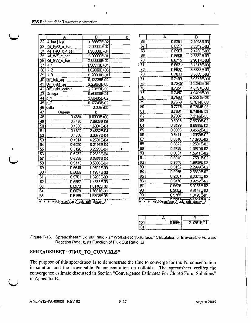
EBS Radionuclide Transport Abstraction
A B 1 c32 U bar[1/yr] 4.36667E-0233 Kd FeO c bar 2.00000E-0134 Kd FeO CP bar 1.96500E+0435 Kd WF c bar 6.00000E-0136 Kd GW c bar I 2.00000E-0237K 1 1.96518E404138 K 2 1.82000E200139 K 3 8.20000E-01140 Diff left aq 9.12736E-02'4__1 Diffrightt.a_q 2.22893E.03[42 Diff fight colloid 2.22893E-0543 Omega 9.50000E-0144 p 1 3.58485E-0245 p. 2 8.17743E-0246 delta 2.00E20047 Om__ea k48 0.4384 0.00002E0049 0.4490 7.8629E-0550 0.4596 1.6034E-0451 0.4702 2.4532E-0452 0.4808 3.3377E-0453 0.4914 4.2591E-0454 0.5020 5.2196E-0455 0.5126 6.2220E-0456 0.5232 7.2688E-0457 0.5338 8.3633E-0458 0.5443 9.5086E-0459 0.5549 1.0709E-0360 0.5655 1.1967 E-0361 0.5761 1.3288E-0362 0.5867 1.4677E-0363 0.5973 1.6140E-0364 0.6079 1.7681 E-0365 0.6185 1.9308E-03
14~c ? -4 Aff
A B66 0.6291 2.1028E-0367 0.6397 2.2849E-0368 0.6503 2.4780E-0369 0.6609 2.6832E-0370 0.6715 2.9017E-0371 0.6821 3.1347E-0372 0.6927 3.3838E-0373 0.7033 3.6506E-03740.7139 3.9373-0375 0.7245! 4.2460E-0376 0.7351! 4.5794E-0377 0.7457: 4.9405E-0378 0.7563 5.3331 E-0379 0.7669 5.7614E-0380 0.7775 6.2304E-0381 0.7881 6.7464E-0382 0.7987 7.3166E-0383 0.8093 7.9503E-03184 0.8199 8.6585E-03185 0.6305 9.4552E-03186' 0.8411 1.0358E-02;87' 0.8516 1.1390E-02r88 0.8622 1.2581E-02;89 0.8728 1.3970E-02 i90 0.8834 1.5611E-02.91: 0.8940 1.7581 -021921 0.9046 1.9989E-02 i931 0.9152 2.2999E-021-E4] 0.9258 2.6869E-02:95 I 0.9364 3.20282-02.96 10.9470 3.9252E-02971 0.9576 5.0087E-02981 0.9682 6.8145E-0299 I 0.9788 1.04262-01-14 4 mj\K-s~urfaceý;aCevdffd~ecEa'L
A I Bi00 0.9894 2.1261 E-01101I
Figure F-16. Spreadsheet "fluxout ratio.xls," Worksheet "K-surface;" Calculation of Irreversible ForwardReaction Rate, k, as Function of Flux Out Ratio, .n
SPREADSHEET "TIMETOCONV.XLS"
The purpose of this spreadsheet is to demonstrate the time to converge for the Pu concentrationin solution and the irreversible Pu concentration on colloids. The spreadsheet verifies theconvergence estimate discussed in Section "Convergence Estimates For Closed Form Solutions"in Appendix B.
ANL-WIS-PA-00000I REV 02 F-27 August 2005

EBS Radionuclide Transport Abstraction
The calculations are done in Worksheet "time to conv," while the plot is in Worksheet"plottime to conv." This description will refer to equations from Appendix B,"Implementation of Radionuclide Sorption onto Colloidal and Stationary Phases with FiniteDifference Solution."
Description of Input Values
The first 29 rows of each worksheet contain the input data values, with the exception of Row 12,where pore volume is computed. Column D contains input values. Column B contains valuesfrom column D that are scaled for unit conversion of mass (kg), length (m), time (yr). An imageof Rows I through 33 is shown on the next page.
Row_2: c-s [kg/mA3]
c, (mg L-U) = Pu solubility
$B$2=$D$2/1000
Row 3: phiI
0_1, porosity of the waste form celll
$B$3=$D$3
Row 4: phi_2
S_ 2, porosity of the corrosion product mass in waste form cell_2
$B$4=$D$4
Row 5: phi_3
S_3, porosity of the invert
$B$5=$D$5
Row 6: u [mA3/yr]
it = volumetric water flux (mi3 yrI)
$B$6=$D$6
Row 7: KdFeOc [mA3/kg]
Kdaeoc, partition coefficient in the FeO colloid state
$B$7=$D$7/1 000
ANL-WIS-PA-000001 REV 02 F-28 August 2005

I I
EBS Radionuclide Transport Abstraction
A I B C 1 D1 Input for Excel sreadsheet Input from GoldSim2 cs ikg/mA31 0.001 o sslgLU 1
3 phi l 1 phL1 14 phi.2 0.4 nhi_2 0.45 phi.3 0.3 uhi_3 0.36 u [m43 /yr] 0.1 ulmA31Vrl 0.1
7 Kd FeO c [mA3/kg] T 1.00000E+01 Kd FeO c_[ml___] 1.0OOOE+048 Kd0FeCP [mA3/kg]' 2.50000E+00 Kd FeO CP lmVglJ 2.50000E+039 Kd WF c_[mA3/kg]jl 2.00000E402'Kd WF c[ml/g]_:: 2.00000E+0510 Kd GW c [mA3_.g] 2.OOOOOE+02 Kd GW c [ml_/g] 2.00000E+05!11 mass Fe0 CP [kg] 1.80000E+04 mass FeO CP [g] 1.80000E+07:12 _Vpore [mA3] 2.29008E+00 V pore [t. 2.29008E+0313 c FeO c [kg/mA3]_ 2.OOOOOE-02 c FeO c Irag/L] 2.OOOOOE+011-4 c FeO CP[kg/mA3] 7.86000E03 c FeO CP rmg/L] 7.86000E+0615 c WF c [kg/mA3] 3.OOOOOE-03 c WF C.[mg/L] 3.OOOOOE+00166 c- GW c [kg/mý_T3 1.OOOOOE-04 c GWc[rag/Lj 1.OOOOOE-0117 rate [_yr] 1.OOOOOE-05 rate [cm_/y! 1.00000E-0318 S FeO c [mA2/kg]_ 1.00000E+05 SFeO C mA2/1 1.00000E+02i1"9 S FeOCP [mA2/kg] 1.OOOOOE-04 S FeO CP[m^2_/gJ 1.OOOOOE+01!20 d FeO [kg/mA3] 5.24000E+03 den FeO [k9gm^A3] 5.24000E+0321 diffusq[mA2yIr] 7.25834E-02 diffus - 2.30000E-09
22 diffus c6lloid [mA_2.yr] 7.258345-04 diffus coloid [•A•2/ 2.30000E-1123 diff.lengthi_[m_] 1.OOOOOE-03 diff length _I_[m] 1.OOOOOE-0324 dEif .L-ength._ _rnm] 5.00000E+00 diff length.2 _[m]j 5.OOOOOE+0025 difflength_3 [I] 8.06000E-01 diff length_3_[m]_ 8.06000E-0126 diff area 1 2 [mA2] 3.60000E-+O1 diff area 1 2 [mA2] 3.60000E+012..7 duff area 23 m.[m2] 1.06800E+00 diff area 2 3 [fm2J 1.06800E+0028 decay_[_yrj 2.87494E-05 decay _1/yr] 2.87494E-0529 delt [yr] 1.OOOOOE+01 delt [y!] 1030 R_bar_ 1 [l/yr] 2.OOOOOE-0231 Rbar_2 [l/yr] 7.86000E+023.2 Ubar [l/yr] 4.36667E-0233 Kd bar FeO c 2.OOOOOE-01
.2An eni~ f "c nA.n14 4 1 N plot timeto cony Xtime to-cony/
Figure F-17. Spreadsheet "time to conv.xls," Worksheet"time to conv;" Summary of Inputs
Row 8: KdFeOCP [m^3/kg]
Kd_FeOCp, partition coefficient in the stationary FeO corrosion product state
$B$8=$D$8/1000
Row 9: KdWF-c [mA3/kg]
Kd_,,,Fc partition coefficient in the waste form colloid state
$B$9=$D$9/1000
ANL-WIS-PA-000001 REV 02 F-29 August 2005

EBS Radionuclide Transport Abstraction
Row 10: KdGW_c [mA3/kg]
Kd G, c partition coefficient in the GW colloid state
$B$10=$D$10/1000
Row 11: massFeOCP [kg]
mFeOCP mass of corrosion products
$B$1 1 =$D$1 1/1000
Row 12: Vpore [mA3]
Vpore = qVbulk m-c , pore volume1-0b PFeOCP
$B$12=$D$12/1000
$D$12=$D$4*$D$11/($D$20*(1 -$D$4))
Row 13: cFeO c [kg/mA3]
CPa._co, concentration of FeO colloids
$B$13=$D$13/1000
Row 14: cFeOCP [kg/mA3]
CPuFeOCP . concentration of FeO corrosion product
$B$14=$D$14/1000
Row 15: cWF c [kg/mA3]
CPU, _;_-c, concentration of waste form colloids
$B$15=$D$15/1000
Row 16: cGW c [kg/mA3]
CPuGIw' c, concentration of GW colloid state
$B$16=$D$16/1000
Row 17: k [mlyr]
k, intrinsic or surface reaction rate (pore-vol/area-FeO/time)
$B$17=$D$17/100
Row 18: S FeO c [mA2/kg]
SFeO-c = specific surface area of FeO colloids (m2 kg-)
$B$18=$D$18*1000
ANL-WIS-PA-000001 REV 02 F-30 August 2005

EBS Radionuclidc Transport Abstraction
Row 19: SFeOCP [mA2/kg]
SFeO cp = specific surface area of FeO corrosion products (mi2 kg-')
$B$19=$D$19*1000
Row 20: d_FeO [kg/mA3]
PFeO CP = density of FeO
$B$20=$D$20
Row 21: diffus-aq [mA2/yr]
Daq = aqueous diffusivity
$B$21 =$D$21 *31558000
Row 22: diffuscolloid [mA2/yr]
Dcotloid = colloid diffusivity
$B$22=$D$22*31558000
Row 23: diff lengthl [m]
L, = diffusive length for cell_1
$B$23=$D$23
Row 24: diff.length.2 [m]
L2 = diffusive length for cell_2
$B$24=$D$24
Row 25: diff.length_3 [m]
L3 = diffusive length for cell_3
$B$25=$D$25
Row 26: diffarea_1_2 [mA2]
=.,12 = diffusive area at cell_1 and cell_2 interface
$B$26=$D$26
Row 27: diffarea_2_3 [mA2]
A, 23 = diffusive area at cell_2 and cell_3 interface
$B$27=$D$27
Row 28: decay [l/yr]
2, decay rate
$B$28=$D$28
ANL-WIS-PA-000001 REV 02 F-31 August 2005

EBS Radionuclide Transport Abstraction
Row 29: delt [yr]
At, time step length
$B$29=$D$29
Rows 30 through 51 contains additional derived parameters for the colloid model. An image ofRows 34 through 61 is shown in Figure F-18.
A I 8 I C [ D I E F G H 7 I____ I____
34 Kd ba-r FeOCP 1.965MEE04OL __ _I____I_ _ _ _ 1_ _ __£ _ _ _
35 Kd-bar WFc -- ý000-01_ _ _ _ _ _ _ _ I_ _ _ O_ _ _ _ _ _ __ _ _ _ _ _ _ _ _ _
36 KdbarCW-c 2.OOOE-02_____ ______ ___
37 K bar I ¶ 9651BE404_________ _____ ____________ ____ __________
38 'K barý 2 1 62C6E4CE______Lt____ _____ ___ ___ ___
39 Kbar 3 8.200E-01 _ _ _ _ _ _ __ _ _ _L_ _ _ _ __ _ _ _ __ _ _ _ _ _ _ _ _ _ _
40 Ddflifta 9_ 912736'0 __[
41 Duf etý __ 9.,ý12736E43J4 -- --- -~i~J42Diffj9th aq 2.22893E-03t_____ I1
243 Dif~fight~colloid 2.22893E-05 _____ ___________1 ______________
44;d~___ __ __ _______2.ii1__E__
I5: 7.1410SE-01_______ _____ ____ _____4____ ____ ____
46s2 5.87541 E-tW _______I_____ ____ ______ ____ ____ ________
47bj69 E.1___________- __________________________
4 b 2 1.39162E-01 __ _ _ __ _ _ _ _ _ _ __ _ _I_ _ _ _ _ _ _ _ _ _
49e 1 e 9.99713Ez-01_ _ _ _ _ _ _ _ __ _ _ _ _ __ _ _ _
50 ýe 2 7.BW74E.03i____ _______I
'1tolerance 1. E-02__________________________________________521 ___________________________ _________________________________
63 deh.time denom a 1 2 a I --- time Pu.aqiyrs)- bj. I delta_1 _ delta2 L ... t_ 2 _ ._Lineyrsj_541 1.0E-03 1.9653E.04 9.9996E.01 115 9.9996E-01 4.5,993E-04 44.2119E-04 1.7578E+05 1.9415E405 19455 _ _1.0E-02 1.9660EE04 9.9960E-01 115 9.9956E-01 4.5975E-04_.4.2104E-.04 1:7682E+04 1.9419E404 194567 1.0E-01 1.9738+04 9______9.9601E.01 115 9.9565E-01 4.5795E-04 4.1952E-04 1.7626E,03 1.9463E403 19557_ 1.0E+W_02.0439E.04 9.6151E-01 I17L±9.5811E-01 4.4068E-4_--4.(499E-04 1.8959E+02_1.9M0EJ402 19958 1.0E84,E01 2.7519E404 7.1411E-01 137A 6.9581E-01 3.2004E-04 3.0078E-04 2.2188E801_2.4083E401 240W9 1.0E.02 9.8328E+04 1.9986E-01 286 1.6616E-01 8.5624E-05 .. 4182E-05 ..5.5709•4O 5.6272E- .. . 50060- 1.. 1.0E+03 _-80641E40.i - 243708.02 1240. 2.2363E-02 _1.0286E-05 1.0265E-05 3.0220E..0 30925E4-0 300061 .OE-04 7.8872E4W6 2.4916E-03 7682 2.2822E-03 1. 0497E-06 1.0495E4-6 2.26133E1-0 222965E-0) - 00
Figure F-18. Spreadsheet "time to_conv.xls," Worksheet time to-conv;" Additional Derived Parametersand Results for Colloid Model
Row 30: R bar.l [l/yr]
R, = SFeO_cCFeO ck, reaction rate constant for colloids
$B$30=$B$18*$B$13*$B$17
Row 31: R bar_2 [l/yr]
R 2 = SFeo CPCFeOcpk , reaction rate constant for corrosion products
$B$31 =$B$19*$B$14*$B$17
Row 32: U bar [1/yr]
U advective rate constant
$B$32=$B$6/$B$12
Row 33: Kd bar FeOc
dimensionless partition coefficient in the FeO colloid state
$B$33=$B$13*$B$7
ANL-WIS-PA-000001 REV 02 F-32 August 2005

EBS Radionuclide Transport Abstraction
Row 34: KdObarFeOCP
dimensionless partition coefficient in the FeO corrosion product state
$B$34=$B$14*$B$8
Row 35: Kd barWFc
dimensionless partition coefficient in the waste form colloid state
$B$35=$B$15*$B$9
Row 36: Kd barGW c
dimensionless partition coefficient in the GW colloid state
$B$36=$B$16*$B$1 0
Row 37: K bar_1
K, =1+ Kd Feo c + -- Feo cp + K-d IT F c + Kd oG,' , combination of dimensionless
partition coefficients
$B$37=1+$B$33+$B$34+$B$35+$B$36
Row 38: K bar_2
K2 =1+KdFeOc +K'--d - combination of dimensionless partition
coefficients
$B$38=1+$B$33+$B$35+$B$36
Row 39: Kbar_3
K 3 =K-FeOc +KdWF_, + KdGJ Vc, combination of dimensionless partition
coefficients
$B$39=$B$33+$B$35+$B$36
Row 40: Diff.leftaq [l/yr]
diffusive rate constant, left interface in water
$B$40=($B$26/($B$23/($B$3*$B$21 )+$B$24/($B$4*$B$21 )))/$B$12
Row 41: Diffleftcolloid [1/yr]
diffusive rate constant, left interface colloids
$B$41 =($B$26/($B$23/($B$3*$B$22)+$B$24/($B$4*$B$22)))/$B$12
Row 42: Diff.right-aq [l/yr]
diffusive rate constant, right interface in water
$B$41 =($B$27/($B$24/($B$4"$B$21 )+$B$25/($B$5*$B$21 )))/$B$12
ANL-WIS-PA-000001 REV 02 F-33 August 2005

EBS Radionuclide Transport Abstraction
Row 43: Diff.right.colloid [1l/yr]
diffusive rate constant, right interface colloids
$B$42=($B$27/($B$241($B$4*$B$22)+$B$25/($B$5*$B$22)))/$B$12
Row 44: denom a_1_2
denominator of Equation B-48
$B$44=$B$37+($B$32*$B$38+$B$40+$B$41 *$B$35+$B$42+$B$43*$B$39+$B$30+$B$31+$B$28*$B$37)*$B$29
Row45: a 1
first coefficient for Equation B-55,a, = __KI
K. + (U-K2+ _ + _oK , _ .c ig taq r Dcight K + 3 I + R+ + AJi2k )At
$B$45=$B$37/$B$44
Row46: a 2
second coefficient for Equation B-55,
a, =(Uj-0 + Kd•_ITc)+Dlef,_-aq +D•ef- colKd- ,fT)AtCsK -+-(U-K -Defiaq left_COIKdWI'Fc- +Dright aq K+ Dight _coK3+R RI +2-It
$B$46=(($B$32*(1 +$B$35)+$B$40+$B$41 *$B$35)*$B$29*$B$2)/$B$44
Row 47: bl
first coefficient for Equation B-58, b,= 1 +- + Dit col + t
$B$47=1/(1 +($B$32+$B$43+$B$28)*$B$29)
Row48: b_2
second coefficient for Equation B-58, b2 = +At
I+ (Uf +Drightcol + ,)t
$B$48=($B$30*$B$29)*$B$47
Row 49: e_1first coefficient for Equation B-64, el -
l+2At
$B$49=1/(1 +$B$28*$B$29)
Row 50: e_2
second coefficient for Equation B-64, e R2At
1 +/2At$B$550=($B$531 *$B$29)*$B$49
ANL-WIS-PA-000001 REV 02 F-34 August 2005

EBS Radionuclide Transport Abstraction
Row 51: convergence relative error tolerance 1% = 0.01.
Rows 54 through 61 calculates the times to converge to limit value for Pu aq concentration andIrrvPu-c concentration as a function of time step size. The time step size (yr) varies by order ofmagnitude increments from I x 10-3 to lx 104.
Column A:delt time
Row 54: assign time step value lxl0-3
Rows 55: $A55 = 10*$A54
This value is dragged down through Row 61
Column B:denom a_1_2
denominator in the calculation for a I and a 2 coefficients.
$B54=$B$37+($B$32*$B$38+$B$40+$B$41 *$B$35+$B$42+$B$43*$B$39+$B$30+$B$31+$B$28*$B$37)*$A54
This value is dragged down through Row 61
Column C:a 1
coefficient in Pu aq concentration Equation B-56.
Row 54: $C54 = $B$37/$B54
This result is dragged down through Row 61
Column D:time Pu aq [yrs]
time for Puaq concentration to converge, estimate Equation B-74.
Row 54: $D54 = $A54*LOG10($B$51)/LOG10($C54)
This result is dragged down through Row 61
Column E: b 1
coefficient in IrrvPu-c concentration, Equation B-59.
Row 54: $E54 = 1/(l+($B$32+$B$43+$B$28)*$A54)
This result is dragged down through Row 61
Column F: delta 1
intermediate tolerance 51 in estimate for IrrvPu-c concentration convergence.
Row 54: $F54 = 0.5*$B$51*ABS(($E54-$C54)/(l-$C54))
This result is dragged down through Row 61
ANL-WIS-PA-00000I REV 02 F-35 August 2005

EBS Radionuclide Transport Abstraction
Column G:delta 2
intermediate tolerance 82 in estimate for IrrvPu-c concentration convergence.
Row 54: $G54=O.5*$B$51*ABS(($E54-$C54)/(1-$E54))
This result is dragged down through Row 61
Column H:t 1intermediate result log'1 (3V) Equation B-75.
log1 0 (b,)
Row54: $H54 = LOG10($F54)/LOG10($E54)
This result is dragged down through row 61
Column I: t 2intermediate result log' 0(82) Equation B-75.
log1 0 (a,)
Row54: $G54 = LOG10($G54)/LOG10($C54)
This result is dragged down through Row 61
Column J: time [yrs]
time for IrrvPu c concentration to converge to given tolerance, Equation B-75.
Row 54: $J54=$A54*INT(MAX(LOG 1 0($F54)/LOG I0($E54),LOG I0($G54)/LOG 1 0($C54)))
This result is dragged down through Row 61.
The plot of the time to converge (shown in Figure F-19) is in Worksheet "plot time to conv"
and is Figure B-5 of Appendix B.
Time to converge for Pu-aq concentration is
x-axis: $A$54:$A$61y-axis: $D$54:$D$61
Time to converge for IrrvPu colloids is
x-axis: $A$54:$A$61y-axis: $J$54:$J$61
Note that the x-axis scale is from 1 x 10⁻³ to I x 10' years, so only Rows 54 through 60 are shownin the figure.
ANL-WIS-PA-000001 REV 02 F-36 August 2005

EBS Radionuclide Transport Abstraction
1 .E+04
1.E+03
1.E+020
,• --E- c_Pu_aq
1.E+01o c irrv Pu c
ý1 .E+O0
1.E-01 1.E+O0 1.E+01 1.E+02 1.E+03
time step size [yrs]
14 • -01%0itt"e .to cmv o tw/ -to.. . . .
Figure F-19. Spreadsheet "time to conv.xls,"Worksheet "plot-time to conv" Plot of Colloid ModelResults
ANL-WIS-PA-000001 REV 02 F-37 August 2005

EBS Radionuclide Transport Abstraction
INTENTIONALLY LEFT BLANK
ANL-WIS-PA-000001 REV 02 F-38 August 2005

EBS Radionuclide Transport Abstraction
APPENDIX G
MICROSOFT EXCEL SPREADSHEET "INVERT DIFFUSION COEFFICIENT"
ANL-WIS-PA-000001 REV 02 August 2005

EBS Radionuclide Transport Abstraction
ANL-WIS-PA-000001 REV 02 August 2005

EBS Radionuclide Transport Abstraction
MICROSOFT EXCEL SPREADSHEET "INVERT DIFFUSION COEFFICIENT"
SPREADSHEET "INVERT DIFFUSION COEFFICIENT" WORKSHEET "MODEL"
The purpose of this spreadsheet is to perform a statistical analysis of the dependence of effectiveinvert diffusion coefficients, D, (cm 2 S-I), on volumetric moisture content, 0 (percent, 100 m3
waterm- 3 bulk volume), as described in Section 6.3.4.1.1. The diffusion data are fit to anequation of the form
eAS.D, = DO ( , (Eq. G-1)
where 0 is the porosity (mi3 void volume m-3 bulk volume), S,, is the water saturation (M3 waterm-3 void volume) (I00 6'S, =0), Do is the self-diffusion coefficient of water (2.299 x 10⁻⁵
cm2 s_') (Mills 1973 [DIRS 133392], Table I11), and the fitting parameter is the exponent, n. Toperform a least squares fit of the data, this equation is linearized in terms of n:
log 10 'I,,Dlog,010 0. (Eq. G-2)( Do 4100)_
Column A, Rows I through 125, of the spreadsheet, shown in Figures G-1 through G-4, containsthe moisture content values, 0 (percent) (Conca and Wright 1992 [DIRS 100436]; Conca et al.1993 [DIRS 170709]), that are listed in Table 4.1-17. The corresponding diffusion coefficientvalues (0S,,D 1 ) listed in Table 4.1-17 are in Column B, Rows 1 through 125 (where they are
labeled D, which represents the effective diffusion coefficient, O,,DI, used in Section 6.3.4.1.1).
In Column C, the quantity 0/100 is computed (e.g., C3=A3/100], and ES,.,D 1 IDO is computedin Column D (e.g., D3=B310.00002299). The log term on the right hand side of Equation G-2,containing the moisture content, is computed Column E (e.g., E3=LOG10(A3)-2). InColumn F, the left-hand side of Equation G-2 is calculated (e.g., D3=LOG1O(D3)).
The least squares fit of the data is done using the Microsoft Excel Trendline tool. In Figure G-5,the results in Column F are plotted on the y-axis against the corresponding values in Column Eon the x-axis in the plot located between Rows 132 and 154 of the worksheet. The type ofregression is linear. The Trendline features, "Set intercept = 0," "Display equation on chart,"and "Display R-squared value on chart" are clicked on. In particular, the "Set intercept = 0"feature results in a fit to Equation G-2, in which the intercept is constrained to be zero.
As shown on the charts, the fitting parameter, n, has a value of 1.863. The correlationcoefficient, R2, is 0.915, indicating a strong correlation between the diffusion coefficient and thevolumetric moisture content. The regression equation is:
S,,Di = DoC 0 (Eq. G-3)(100)
ANL-WIS-PA-00000I REV 02 G-1 August 2005

EBS Radionuclide Transport Abstraction
In Column G, the error, or deviation of each data point from the fitted equation, is calculated(e.g., G3=F3-1.862899*E3)); i.e., for data point i, the calculation in Column G is thedeviation ci
ei = logl04•-( %D1 -1.8631logl 1o 0 (Eq. G-4)
In Cell G128, the average of the 125 values of e, is computed: G128=AVERAGE(G3:G127).
The standard deviation of the gi,, Cell G129 is computed: G129=STDEV(G3:G127).
F - A r, n C I C" -
t91100 DIOtlogi 01(1
j -1.0 1 9E-W0.0150 6.046E-04 3.14 1,70 .60E-090.0170 i2.871 E-04 -,75 1.90-, UOE-09 0.0190 1 3.741 E-04 -. 2 a26 2.17 217EM ~0.0217 1,205E-03 -,6 1197 2.20 3.63E438 0.0220 1.579E-03 -. 9 .0
4 -2.29 -TO-9-E-W0.0229 4 .741 E04 W 22.60 2,GE-138 0.0250 1.087E-03 1.6m -,6
10 3.103.30E-M 0.0310 1.435E-03 -1" -2411 3.14 3.06E-M0.0314 1.331 E-03 1.0 Z-i 2 3 2 1 -3 E - B0 .0 3 2 0 5 . 7 2 E 6 4-1 9 63 , 113, 3.272.79E-M0.0327 1.214E-03 -145-.1'f4 3,3 6.5EM0.0333 2.762E-03 1.4715 3.34 2.60E-080.0334 1. 1131 E.03 -14.--416 3.57 .37E-090.0357 1.466E-03 -147 -- 317 3.70 3.70E-08 0.0370 1.609E-03 4 42 ZM18 3.70 .60E-060370 2.871 E-03 -. 43 Z19 4.0 ra.2E.W0.0400 2.271 E.03 -1,*620 4.0 519E-OB0.0420 2.584E4:03 -13.'s21 4.0 6ý2 E-080.0460 2.701 E-03 -.22 4 90 ý20E -W ý , O Mo 9 3.132E -03 - 1 3 0- . Ný3 5.10 ý1-32E-07 0.0510 5.742E-03 -. 292 .Z424 5,30 ,4OE438 0.0530 1.044E-03 -126.Z8
-6.40 T6OE4)B 0.0540 3.306E-03 -. 2E 241261 5.51T68E-W 1 0.0551 3.341 E-03 -120iV27: 5.831.23E-07 0.0583 5.350E-03 -1214 47
5.90~~ ~ 0.0590 4.045E-03 -129 Z9
29' &00 .92E-08 0.0600 3.880E-03 122 16.30 1.06E-07.0630 4.611 E-03 - .0,i.3
31 &90 6.UDE-08 0.03690 2.610E-03 11 -. 1332 6931.0E 070.0693 6 65_'_'_''_'_11_'_'_5E433
Figure G-1. Spreadsheet "Invert Diffusion Coefficient," Worksheet "Model;" Invert Diffusion CoefficientInput Data (Water Content 1.50 to 6.93%)
ANL-WIS-PA-000001 REV 02 G-2 August 2005

0EBS Radionuclide Transport Abstraction
A B C D --- E F G0.073 T309160E-3
7.40 250E-G7 0.0740 1.087E-02 -,117.60 2-60E-070760 1. 131 E-02 -,4'761) -1.10E-07 0.0760 4.785E-03 -. 1* - 2
37 7.0 2.6E-07 0.0760 1.170E-02 . j9 -1338 7.70 1- 1 OE-07 0.0770 4.785E-03 114 -2T
8.00 0.1B80 8.612E-03 -ýP'6ý0- 1 B-1 1.70E-07 0.0810 7.395E-03 -102 Z1341 32 IOE07 0.0832 1.783E-02_ -. 0 -. 4-42 8,5 2.1E-07 0.0835 9.352E-03 -. 7
B.60 3.20E-07 0.0%60 .1.392E-02 -. 6 1668.80 2.30E-07 0.0880 1.000E-02 1A2.09.24 ~~0.0924 1.ý109E-02 -134 1.6
461 9.24 2.55E-07 0.0924 .1.109E-02 -. 04 1.9547- 1 9ý5 3.90E-0 0.0956 1.305E-02 -. 4- 8
48 9.64, 3NE-07 0.0964 1.335E-0 106 18449' 9.751F20E-07 0.0975 1.392E-02 -. 1 18
60 1.1G; Bl -0 0.1010 I.SV-.9_ýýi 1 1,16, 7362E-57 0.1616 1.575E-62 79* 8
-521 10,20 3.54E-0 0.1020 .1.540E-02 _ -- 9, -,1531 10.2 33OE-07 0.1020 1.435E-02 -~ý -. 4647 10-30 3.-34E-07 0.1030 ""1.453E-02 -"97 IM
2._O 0.1030 9,244356 40140_0 0.1040 1.479E.-02 -- 8 1857 1O.W,3;62E-07 0.1090 1.575E0 -093 .058 11.10.:3.T2E-070.1110 - 1.618E-02 -096."959 11.1GI,4.2E-0 0.1110 1.836E-02 096-.3so 1110ý k7E-07 0.1110 1.85E-02 . 0ý .. 361_1 111Z, 0.1120 1.823E-02 -- 91173621 11,20 ýýE.48&67 0.1120 .2.384E-02 -. 91 1.3
11 114404.27E-0 0.1140 1.B57E-MO2 .U 1.364' jjý 40 4,12E-0 0.1140 .'1.792E-02 -- 4 177
ýý-'ýtt'50'411__ _0.160 _2.349E -02 _ 096 1.2
Figure G-2. Spreadsheet "Invert Diffusion Coefficient," Worksheet "Model;" Invert Diffusion CoefficientInput Data (Water Content 7.30 to 1 1.60%)
ANL-WIS-PA-000001 REV 02 G-3 August 2005

EBS Radionuclide Transport Abstraction
A B C D E F G6 '1 0,1160..._. 1... 2 .349E-021.2
o1_011 1.131E-020.1180 2.083E-02
681 12,W 2 40E-07 0,1200 1.044E-02 -09t 1.1W 12.00- 0.1200 1.944E-02 4.2 .1
0.12120 T.7E-02
0.1230 2.197E-0272 7,30 0,1230 1.914E-02 -. 1 17T3 12.300,1230 1.566E-0 ai
0.1230 1.95-E.0270.1250 1.261E-02
Inpu D (Wte C:4Eontent 0.1270 t 1.901E-02-i7 '2.7 ý,,,A90-07, 0.1270 i 2.131 E-02 M-
78 ý532E-OV",- 0.1270 2.314E-0 0M4.77 0.1310 2.a75E-0 083 -,8
80 13.906.39E-G7 0.1390 2.'344E-0 a ,6W
62 1400 ~0,1410 2.22E-0 G86 IU83, 14.0&52E-07 O. 1420 2,401 E-0 W-'84 14,40-4,50E-07, 0.1440 1.957E-0 OO .0
14.40 5,2DE-ýO0.1440 2.26:2E-02 -. 4 .14,0 450E07 0.144 1,ý957E-0 82 4714.60 6,82E 7 0.1466 2,9b7E -. % -,2
88 14.70 ,OOE-071470 3.915E-02 QM.0891, 1480,: 654E-07 0.1480 2.845E-3 • .U -1sgo 16.00 1,47E-06 0.1600 6.394,E-0 0% -. 991 -16,1u&82E-07: 0.1610 2.967E43 o73 -. 292 1-06.4E-0 0165.._0__ 2,371 E-0293 16.70&WE-07. 0.1670 2.871 E-02 -. 494 17. ~~JT00 1500. 20E Q2 -070 1m95 171 2E-7,,: 0.1710 1%67-96 1,39 ,76E06,:'9; 0.1730 7.6 E-2 -. b
Figure G-3. Spreadsheet "Invert Diffusion Coefficient," Worksheet "Model;" Invert Diffusion CoefficientInput Data (Water Content 11.60 to 17.50%)
ANL-WIS-PA-000001 REV 02 G-4 August 2005

EBS Radionuclide Transport Abstraction
A 8 flDE F H IEBS
Radionuclide
Transport Abstraction
99
101010
10
ý12
1t2
17.50 1.1GE4)5 OA6 4.iý4ýdf -GJý -1 ý=m8d 1.60E-06 0.188D 6.960E-02 -0.726 -1.167IR90 B. 19EX 0.1890 3.562E-02 Z124 .11
0 1940 9.89E-07 0.1m 4.302E-02 -0.712 'IJ661 20,40 4.19E-06, 0.2040 1.823E-01 -O.m2 20,80 3.58E436 0.208D 1.557E-01 -0182 -OAM3 21-00 2.34E-06 0,2100 1.018E-01 .0.6M -W9924 21 ý50 1ý23&06 0.2150 5.350E-02 -1,2726 21,60 1.29E-06 0,2160 5.611E-02 OM -1,251
2.4OEa 0.2310 1.0"E-01 -UH36 -al7: 23,10 1.90E-06 0.2310 8,264E-028 24.GO 2.9OE4)6 0.2400 1.261E-01 _U20 m9 2-530 5.62E-06 0.2530 2.532E-01 -0.597 1 OW0 2540 2 50E-06 0.2540 1.087E-01 46% -019641 2570 9.26E-06' 0.2570 4MBE-01 r;ýU- -03952 28,20 3,SOE-06 0.2820 1.522E-01 46W 48173 20,50 1,0DE-06 0.20W 4.350E-02 41546 -tý 3624 30,90 t4 51 E-06 0.3090 6.5WE-02 -1.1835' 31.70 1.23E-05 0.3170 5.350E-M -0.499 -0.2726 32.30 4.60E-06 0.3230 2.001E-01 44917! 33,80 1.34&06 0.3380 &829E-01 -OA -0,2348ý 35-80 1,57E-05 635M &WE-01 44469 33E-06 0.38M IME-01 -0.7250 .30 1.36E-G5 0.39m 5.916E-01 -0,406 -0.1 39,rQ 1A3E4)5 0,39M I 4.916E-01 -0.403 43082 4000 6.90E-06 0.4000 1 3.001 EV -01396 -0.5n3 42,010 5. 8GE-06 OA200 ZS23E-01 407 45904 4-2.50 3.22E-06 0.4250 1.401E-01 -O.-M -G.8545 0.4340 4.437E-01 -0.36346 _,!Oo 0.49M ZBO&OT -6 310 a57-717 66 30 1ý83E-OFY 0.663D 7.960E-01 -_04178 -U99
Figure G-4. Spreadsheet "Invert Diffusion Coefficient," Worksheet "Model;" Invert Diffusion CoefficientInput Data (Water Content 17.50 to 66.30%)
ANL-WIS-PA-000001 REV 02 G-5 August 2005

EBS Radionuclide Transport Abstraction
1ý7
132133
136
133
134
1435
147
149140
143144
A 1 B 1 C I D I
•ute. Conoa and V 1992k Con•a et al 193
-1
0.0 ,
-0.5
-1.0 * Conca and Vright (1992)Conoa et al. (1993)
-1.5 • Linear (Conca and Wright(1392t- Conca et al. (193))
•l .2.0
.- 25
-3.0
-3.5
-4.0-2.0 -1.5 -1.0 -0.5 0.0
Ioglef - 2
Source: Conca and Wright 1992 [DIRS 100436]; Conca et al. 19b3 [DIRS 170709].
Figure G-5. Spreadsheet "Invert Diffusion Coefficient," Worksheet "Model;" Plot of Fitted Invert DiffusionCoefficient Data
In the plot in Figure G-6 between Rows 169 and 191, the lines for the mean and for the meanplus or minus three standard deviations are added to the plot shown earlier. The lines are drawnover the range of the data, i.e., for 0/100 from 0.015 to 0.663 (Column C, Rows 159 to 166).
The y-values for the Trendline fit are computed as VSwDI / Do = (0 / 100)1.863
(e.g., D159=(C159A^ .863)), and the values plotted are log10(OSwD 1 I DO)
(e.g., G1 59=LOG1 0(D159)). For the mean curve, the y-values are computed as
,SwD, / D, = (0 / 100)1863 100033 (e.g., D163=(C163^1 .863)*1OA(0.033)), and the values plotted
are again logo(SwD, IDo) (e.g., G163=LOG10(D163)). For the mean plus three standard
deviations curve, the y-values are computed as qASwD1 / Do = (0/100).863100033+3(0218)
(e.g., G161=(C161A1.863)*1OA(0.033+3*0.218)), and the values plotted are again
log1O(•wD•Do1 D0 ) (e.g., G161=LOG10(D161)). The mean minus three standard deviations
curve is done similarly. This plot is shown as Figure 6.3-4 in Section 6.3.4. 1. 1.
ANL-WIS-PA-000001 REV 02 G-6 August 2005

EBS Radionuclide Transport Abstraction
157-ý
158i
160161
163164
1676
169:1701711172~173174;
176i
177
179
.1811182183 1
185
1871688189190191
194:
A C D E F 0 -H, ]_ I
Lines for plot at ± 3 standard deviationsloglO(q/1 00) 6'1lO0 DjD1D0 =(t1OO)1
loga( D IO)-1.8239 0.015 4.000E-04 Trendline -3.3979-0.1785 0.663 4.650E-01 Trendline -0.3325-1.8239 0.015 1.946E-03 mean + 3 std dcv -2.7109-0.1785 0.663 2.262E+00 mean + 3 std dav 0.3545-1.8239 0.015 4.316E-04 mean -3.3649-0.1785 0.663 5.017E-01 mean -0.2995-1.8239 0.015 9.573E-05 .mean - 3 std dev -4.0189-0.1785 0.663 1.113E-01 mean-3stddev -0.9535
1.0
0.5. 0 Conca and Vkight (1992);
0.0 .Conca et al. (1993)
Mean-0.5
-1.0 - - - Mean+3s
9 -1 .5- - - Mean - 3s
-2.0
-2.5 - Linear (Conca and tight(1992); Conca at al. (1993
-3.0
-3.5
-4.000
I001g& - 2
Source: Conca and Wright 1992 [DIRS 100436]; Conca et al. 1993 [DIRS 170709].
JA41i
Figure G-6. Spreadsheet "Invert Diffusion Coefficient," Worksheet "Model;" Plotted Results of InvertDiffusion Coefficient Data, Showing Uncertainty Range as Mean ±3 Standard Deviations
The data are further analyzed in Figure G-7 to demonstrate that the deviations approximatelyfollow a normal distribution. Under the Microsoft Excel menu item Tools, Data Analysis... isclicked, and Histogram is selected under Analysis Tools. In the Histogram window, the errordata (Column G, Rows 3 to 127) are entered for the Input Range. For the Bin Range, Column I,Rows 3 to 22, is entered. The frequency distribution is output in Column J, Rows 3 to 22. Forcomparison, a theoretical normal distribution is computed over the same range in Column M:
1 -(x-l,)2 / 202f (x;l,,cr) 2 e (Eq. G-5)
where x is the bin value, the mean p di 0.033, and the standard deviation a u 0.218.
ANL-WIS-PA-000001 REV 02 G-7 August 2005

EBS Radionuclide Transport Abstraction
The Microsoft Excel formula is (for Cell M3, for example):
M3=EXP(-((13-0.0329438386573088)A2)/(2*0.218121819319092 A2))/
(0.218121819319092"(2"P1())AO.5)
20 h%3 0 344 0.1 25 0.2~ 1s6 -0.1 147 -0.2 10
80.3 t09 0.6 3
11 -0.41 212 0.4! 213 6.5. 214 -0.6 115 -0.3 1160.6! 1Is117 -ti 018 -0.9 0
1-071 020-0.7 0
21 -0.5 022 0.9 023 I 024 More 0 More 0252627 40 2.0
289351.8
_ 1.630 !.4
31 01.432
325 1.2
20 1.0 [ om Dtru35 -a- Norma D
37 0.638 10 04
5 0.43940 0 2
0.041 0 -0.043
Bin
Figure G-7. Spreadsheet "Invert Diffusion Coefficient," Worksheet "Model;" Further Analysis of InvertDiffusion Coefficient Data
ANL-WIS-PA-000001 REV 02 G-8 August 2005

EBS Radionuclide Transport Abstraction
SPREADSHEET "INVERT DIFFUSION COEFFICIENT"WORKSHEET "VALIDATION"
In this worksheet (Figure G-8), diffusion coefficient data (Column B) from Tables A-I and A-2of The Determination of Diffusion Coefficient of Invert Materials (CRWMS M&O 2000[DIRS 156680]) are plotted against water content (Column A), along with the results of theanalysis in Worksheet "Model." The purpose of this worksheet is partially to validate thediffusion coefficient submodel by showing that the model overestimates the value of the invertdiffusion coefficient, thereby overestimating diffusive releases of radionuclides through theinvert. The model curve fit (Equation 6.3.4.1.1-22), also shown on p. G-7 and in Figure 6.3-4 inSection 6.3.4.1.1, is reproduced in Columns D-G, Rows 3 and 4, and plotted in the figure below.
C H K
1.E-04
1 .E-05
. CRYS M&O 2O000
l.E-06
- ESS RTA Model (Mewn)(Eq~ation 7.2.2.2-1)
-1 EBS RTA - 3 std dev
1 .E-08 - -EBS RTA- 3 std dev
0.1.E-09
0.10 1.00 10.00 100.002930 Source: CRWMS M&O 2000, Tables A-1 &A-2131
3436
3i42..
Water ConteI ([%)
1±1.. ,.l k]
Source: CRWMS M&O 2000 [DIRS 156680], Tables A-1 and A-2.
Figure G-8. Spreadsheet "Invert Diffusion Coefficient," Worksheet "Validation;" Validation of InvertDiffusion Coefficient Data
0ANL-WIS-PA-000001 REV 02 G-9 August 2005

EBS Radionuclide Transport Abstraction
INTENTIONALLY LEFT BLANK
ANL-WIS-PA-000001 REV 02 G-10 August 2005

EBS Radionuclide Transport Abstraction
APPENDIX H
QUALIFICATION OF DIFFUSION COEFFICIENT DATA
ANL-WIS-PA-000001 REV 02 August 2005

EBS Radionuclide Transport Abstraction
0
ANL-WIS-PA-000001 REV 02 August 2005

EBS Radionuclide Transport Abstraction
QUALIFICATION OF DIFFUSION COEFFICIENT DATA
DESCRIPTION OF DATA TO BE QUALIFIED
The data reported in Conca and Wright (1992 [DIRS 100436]) and Conca et al. (1993[DIRS 170709]) consist of measured diffusion coefficients of unsaturated soil, gravel, bentonite,rock, and crushed tuff from Yucca Mountain, over a broad range of water contents. These datahave been collected and analyzed using standard scientific practices. The diffusivity data forvarious granular media at volumetric moisture contents ranging between 1.5% and 66.3% aregiven in Section 4.1.2, Table 4.1-17. These measured data have been used to analyze thedependence of the diffusion coefficient on volumetric moisture content for a variety of granularmaterials (Section 6.3.4.1.1). These data are qualified in accordance with the data qualificationplan included in this appendix.
CORROBORATING DATA
The diffusion coefficient data for crushed tuff materials from The Determination of DiffusionCoefficient of Invert Materials (CRWMS M&O 2000 [DIRS 156680]) are used to qualify thedata reported by Conca and Wright (1992 [DIRS 100436]) and Conca et al. (1993[DIRS 170709]). The diffusion coefficient data found in The Determination of DiffusionCoefficient of Invert Materials (CRWMS M&O 2000 [DIRS 156680]) were collected in theDOE Atlas Facility. The tests were performed by the EBS Testing Department underYMP-approved procedures using the Unsaturated Flow Apparatus. The Unsaturated FlowApparatus method is reported to be an accurate and fast indirect method of determining diffusioncoefficients in porous media (Conca and Wright 1992 [DIRS 100436], p. 7). The method usesmeasurements of electrical conductivity, at specified volumetric moisture content, which isconverted to diffusion coefficient. The Determination of Diff/ision Coefficient of InvertMaterials (CRWMS M&O 2000 [DIRS 156680]) reports that the error on the reported data iswithin ±7%. The reported data are shown in Table H-1.
DATA EVALUATION CRITERIA
The diffusion coefficient data from Conca and Wright (1992 [DIRS 100436]) and Conca et al.(1993 [DIRS 170709]) will be considered qualified if they are within one order of magnitude ofthe values reported in The Determination of Diffusion Coefficient of Invert Materials(CRWMS M&O 2000 [DIRS 156680]); or if greater differences are observed, they result inmore conservative results with regard to radionuclide releases.
COMPARISON OF THE DIFFUSION COEFFICIENT DATA IN CONCA ANDWRIGHT (1992 IDIRS 1004361) AND CONCA ET AL. (1993 IDIRS 1707091) TO CRWMSM&O (2000 IDIRS 1566801)
The data reported by Conca and Wright (1992 [DIRS 100436]) and Conca et al. (1993[DIRS 170709]) (shown in Section 4.1.2, Table 4.1-17) consist of diffusion coefficient data forthe range of 1.5% to 66.3% volumetric moisture content. The data from The Determination ofDiffusion Coefficient of Invert Materials (CRWMS M&O 2000 [DIRS 156680]) rangesbetween 0.2% and 32.13%. Figure H-I shows a plot of moisture content versus diffusioncoefficient for data from both sources. The figure shows that overall the Conca and Wright
ANL-WIS-PA-000001 REV 02 H-1 August 2005

EBS Radionuclide Transport Abstraction
(1992 [DIRS 100436]) and Conca et al. (1993 [DIRS 170709]) data have higher diffusioncoefficient values over the measured range of water content. The differences are highest at lowwater content. At water content values below 10%, the Conca and Wright(1992 [DIRS 100436]) and Conca et al. (1993 [DIRS 170709]) diffusion coefficient values arehigher by as much as two orders of magnitude. For water content values above 10%, the Concaand Wright (1992 [DIRS 100436]) and Conca et al. (1993 [DIRS 170709]) diffusion coefficientdata show higher but comparable values.
The differences in diffusion coefficient at low water content values can be partly attributed to themeasurement technique. As discussed in Section 6 of The Determination of Diffitsion Coefficientof Invert Materials (CRWMS M&O 2000 [DIRS 156680]), errors in measurement are higher atlow diffusion coefficient values. Conca and Wright (1992 [DIRS 100436], p. 10) also reportedthat, at low water content, reductions in water content result in sharp declines in the measureddiffusion coefficient as surface films become thin and discontinuous, and pendular waterelements become small. Measurement differences could also be attributed to the different porousmedium samples used. The Conca and Wright (1992 [DIRS 100436]) and Conca et al.(1993 [DIRS 170709]) data include various material samples whereas the determination report(CRWMS M&O 2000 [DIRS 156680]) data are for crushed tuff only. The data from bothsources show some scatter. The diffusion coefficient data of Conca and Wright(1992 [DIRS 100436]) and Conca et al. (1993 [DIRS 170709]) are thus comparable to those ofthe determination report (CRWMS M&O 2000 [DIRS 156680]) for volumetric water contentvalues above 10%. For low volumetric water content values, the differences are greater.However, the higher diffusion coefficient values of Conca and Wright (1992 [DIRS 100436])and Conca et al. (1993 [DIRS 170709]) will result in predicted radionuclide releasesbeing higher.
The Conca and Wright (1992 [DIRS 100436]) data have been published in a peer-reviewedjournal (Applied Hydrology), and thus have undergone strict review. The data are shown plottedin Figure 2 of Conca and Wright (1992 [DIRS 100436]).
The Conca et al. (1993 [DIRS 170709]) data have been published in the proceedings of theScientific Basis for Nuclear Waste Management XVI Symposium held November 30 toDecember 4, 1992. This symposium was organized by the Materials Research Society, whichwas formed in 1973. The most recent Scientific Basis for Nuclear Waste Management XVISymposium is XXVII, the proceedings of which were published in 2004. Papers published in theproceedings undergo peer review prior to publication and must be presented at the meeting inorder to be published.
SUMMARY OF QUALIFICATION
The diffusion coefficient data of Conca and Wright (1992 [DIRS 100436]) and Conca et al.(1993 [DIRS 170709]) have been evaluated in the context of their use in radionuclide transportmodeling, and are considered qualified for use within this report per LP-SIII.2Q-BSC,Qualification of UnqualifiedData, Attachment 3, on the basis of:
Availability of corroborating data-The corroborating data are YMP-generated data usingthe same measurement technique.
ANL-WIS-PA-000001 REV 02 H-2 August 2005

EBS Radionuclide Transport Abstraction
" Reliability of data sources-The data are published in a peer-reviewed journal and in apeer-reviewed symposium proceedings.
" Data demonstrate properties of interest-The published data, diffusion coefficients incrushed rock, are the data required for the model of transport in the invert.
The above comparison of the diffusion coefficient data of Conca and Wright(1992 [DIRS 100436]) and Conca et al. (1993 [DIRS 170709]) with the corroborating data fromCRWMS M&O 2000 [DIRS 156680] shows that the data evaluation criteria have been met. Thedata to be qualified are within one order of magnitude of the values in the corroborating sourcefor volumetric water content values above 10% (Figure H-I). The differences between the twodata sets are greater than one order of magnitude below 10%; however, the higher diffusioncoefficient values of Conca and Wright (1992 [DIRS 100436]) and Conca et al.(1993 [DIRS 170709]) will result in predicted radionuclide releases being higher. Therefore, theConca and Wright (1992 [DIRS 100436]) and Conca et al. (1993 [DIRS 170709]) diffusioncoefficient data shown on Table 4.1-17 are judged to be qualified for use in this report. Use ofthese data in other applications would require a comparable evaluation for that specific use.
Table H-1. Diffusion Coefficient of Crushed Tuff Invert Materials
Volumetric Moisture Diffusion CoefficientSample Content (%) (cm 2 s-1)
1 32.13 2.02 x 10-62 18.15 5.40 x 10-73 9.26 4.05 x 10-84 7.03 6.75 x 10-95 6.97 7.45 x 10-96 6.89 6.73 x 10.97 6.75 5.42 x 10-98 6.63 4.39 x 10-99 6.63 3.76 x 10-910 6.23 3.40 x 10-911 6.00 3.43 x 10-912 5.55 2.04 x 10-913 5.46 2.04 x 10⁻¹⁴ 8.29 2.24 x 10-915 7.54 6.81 x 10416 7.36 6.21 x 10417 7.22 4.38 x 10-918 6.84 2.19 x 10-919 6.11 1.55 x 10-920 5.41 9.97 x 10-'021 4.45 6.19 x 10⁻¹⁰
22 3.64 5.00 x 10-1023 0.29 1.24 x 10⁻¹°24 0.20 1.25 x 10-'0
Source: CRWMS M&O 2000 [DIRS 156680].
ANL-WIS-PA-000001 REV 02 H-3 August 2005

EBS Radionuclide Transport Abstraction
1.E-04
l.E-05 ÷ 4 •
A-4
E 1.E-06
4a1.E-07.--l; * Conca and Wright (1992);
. W. Conca et al. (1993)
2 1.E-08 - CRWMS M&O (2000)o
1 .E-09
1.E-10
0 10 20 30 40 50 60 70
Volumetric Moisture Content (9/4
I I
Source: Conca and Wright 1992 [DIRS 100436]; Conca et al. 1993 [DIRS 170709]; CRWMS M&O 2000[DIRS 1566801.
Figure H-1. Comparison of Diffusion Coefficients
DATA QUALIFICATION PLAN
A facsimile of the data qualification plan developed for the above qualification effort is providedin Figure H-2. The original is included in the records package for this model report.
ANL-WIS-PA-00000I REV 02 H-4 August 2005

4
EBS Radionuclide Transport Abstraction
Data Qualification Plan QA: QABSC Page i ofi
Complete only appLkabe Items.
Section I. Organizational InformationOuardication Title
QUALIFICATION OF DIFFUSION COEFFICIENT DATARequesting OrganizationNear-Field Environment and Transport
Section II. Process Planning Requirements1. List of Unquaklfed Data to be Evaluated ,,Diffusion coefficient data reported in Conca and Wright (1992 [DIRS 100436]) and Conca et al. (1993 [DIRS 170709]). These dataare shown on Table 4.1-17 of this report.
2. Type of Data Quarntcatlon Mettod(a) [Induding rationale for selection of method(s) (Attadcinent 3) and quafifcation attributes (Attachment 4))Qualification method, from Attachment 3 ofLP-SIII.2Q-BSC, REV 0 ICN 0: Corroborating Data. The diffusion coefficient data forcrushed tuff materials from the Determination of Diffusion Coefficient of Invert Materials (CRWMS M&O 2000 [DIRS 156680]) areused to qualify the data reported by Conca and Wright (1992 [DIRS 100436]) and Conca et al. (1993 [DIRS 170709]).
Attributes used from Attachment 4: (3) The extent to which the data demonstrate the properties of interest, (8) Prior peer or otherprofessional review of the data and their results; and (10) Extent and quality of corroborating data.
3. Data Qualificatlon Team and Additional Support Staff RequiredChairperson: James Schreiber, Sandia National LaboratoriesTechnically competent individual: Teklu Hadgu, Sandia National Laboratories
4. Data Evaluation CriteriaThe diffusion coefficient data from Conca and Wright (1992 [DIRS 100436]) and Conca et al. (1993 [DIRS 170709]) will beconsidered qualified if they are within one order of magnitude of the values reported in CRWMS M&O 2000 [DIRS 156680]; or ifgreater differences are observed, they result in more conservative results with regard to radionuclide releases.
5. Identification of Procedures UsedLP-SIII.2Q-BSC, Qualification of Unqualified DataLP-SI1I.! 0Q-BSC, Models
Section Ill. Approval
Oualification Chakperson Printed Name Ouatfication C son, ur . Date •
James Schreiber 8/24/05Responsible Manager Printed Name es lo/4anager,•gna•ure Dale
Ernest Hardin 8 8/24/05
LP-S11120-8SC FORM NO. LS1112.1 (Rev. 01119r2005)
Figure H-2. Data Qualification Plan
ANL-WIS-PA-000001 REV 02 H1-5 August 2005

EBS Radionuclide Transport Abstraction
INTENTIONALLY LEFT BLANK
ANL-WIS-PA-000001 REV 02 11-6 August 2005

EBS Radionuclide Transport Abstraction
APPENDIX I
COMPARISON OF OUTPUT DTNS
ANL-WIS-PA-00000I REV 02 August 2005

EBS Radionuclide Transport Abstraction
ANL-WIS-PA-000001 REV 02 August 2005

EBS Radionuclide Transport Abstraction
COMPARISON OF OUTPUT DTNs
The output from this report consists of three preliminary output DTNs: SN0403T0507703.015,SN0409T0507703.017 and SN0503T0503305.001, and three final outputDTNs: SN0410T0507703.018, SN0508T0503305.003, and MO0506SPAINPAR.000. In thisappendix, the differences between two preliminary output DTNs (SN0403T0507703.015 andSN0409T0507703.017) are discussed. In addition, the final output DTN: SN0410T0507703.018is compared with the second preliminary DTN: SN0409T0507703.017. These comparisonsprovide traceability for TSPA-LA applications that were initially developed based on thepreliminary output DTNs.
The output in the three DTNs discussed in this appendix consists of tables from Section 8(Conclusions) of the EBS RT Abstraction. Each of these tables is compared in this appendix.Numerous editorial revisions were made in converting the first preliminary version of the DTNto the second preliminary version; because these editorial revisions have no impact on TSPA-LAresults, they are not discussed in this appendix.
TABLE 57 (DTN: SN0403T0507703.015) VS. TABLE 8.1-1 (DTN: SN0409T0507703.017)
Table 57 (Summary of EBS Flow Abstraction) in DTN: SN0403T0507703.015 corresponds toTable 8.1-1 in DTN: SN0409T0507703.017. The key differences in this table between the twoDTN versions are the expressions for the flux through the drip shield, F2, and the flux into thewaste package, F 4. In preliminary DTN: SN0403T0507703.015, F2 is expressed as:
F2 = FILDSPatchfDS /(2LDs). (Eq. I-1)
The parameters are defined in the Table 57 in DTN: SN0403T0507703.015. This equation istechnically correct, but it is expressed more completely in DTN: SN0409T0507703.017 as:
F2 = min[FiNbDsLDspachfDs/(2LDs), F1]. (Eq. 1-2)
The parameters are defined in the Table 8.1-1 in DTN: SN0409T0507703.017. Equation 1-2replicates Equation 6.5.1.1.2-37 in the EBS RTAbstraction. Equations I-I and 1-2 give the sameresult when the number of corrosion patches in the drip shield, NbDs, is one, which is the case inthe WAPDEG model of drip shield failure (BSC 2004 [DIRS 169996], Section 6.3). The minfunction in Equation 1-2 provides a numerical check to prevent an unrealistic result of F 2 > F,from being obtained if the parameter values used in the equation were to give that result.
The same discussion applies to the flux into the waste package. InDTN: SN0403T0507703.015, F 4, is expressed as:
F4 = F2L,,,p p ,,fjp/(2L1,,,). (Eq. 1-3)
The parameters are defined in the Table 57 in DTN: SN0403T0507703.015.
ANL-WIS-PA-000001 REV 02 1-1 August 2005

EBS Radionuclide Transport Abstraction
This equation is technically correct, but it is expressed more completely inDTN: SN0409T0507703.017 as:
F 4 = min[F2Nb,,,pLa,,L WI,,ahf' 1(2L;rp), F2 ]. (Eq. 1-4)
The parameters are defined in the Table 8-1 in DTN: SN0409T0507703.017. Equation 1-4replicates Equation 6.5.1.1.3-1 in the EBSRTAbstraction. The difference between Equations 1-3and 1-4 is the definition of Lp _Patch. In Equation 1-3, Ljvp_Patch, is the length of all corrosionpatches in the waste package, whereas in Equation 1-4, L Pa,,tch is the length of each corrosionpatch; thus, the product NbwpLwvpPatch in Equation 1-4 is equal to L?_p,,Path in Equation 1-3. Themin function in Equation 1-4 provides a numerical check to prevent an unrealistic result ofF4 > F2 from being obtained if the parameter values used in the equation were to give that result.
In the Flow Parameter column for Flow Pathway 8 in Table 57 in DTN: SN0403T0507703.015,a flux F9 is erroneously included in the equation and is deleted in the final DTN. Since this fluxdoes not exist, its inclusion in the preliminary DTN has no impact on the TSPA-LA calculation.
The references and comments in the Data Sources & Notes column in Table8.1-1 inDTN: SN0409T0507703.017 are updated from Table 57 in DTN: SN0403T0507703.015; theseupdates have no impact on TSPA-LA calculations.
TABLE 58 (DTN: SN0403T0507703.015) VS. TABLE 8.1-2 (DTN: SN0409T0507703.017)
In DTN: SN0409T0507703.017, the cross-sectional area for radionuclide transport is clarified inTable 8.1-2, with references to sections in the report. In DTN: SN0403T0507703.015, the sameparameter is referred to as the flow cross-sectional area in Table 58 and described in vague termsthat prompted a revised description in the final DTN. References are updated inDTN: SN0409T0507703.017, Table 8.1-2. None of these changes has any impact onTSPA-LA calculations.
TABLE 59 (DTN: SN0403T0507703.015) VS. TABLE 8.2-1 (DTN: SN0409T0507703.017)
In Table 57 in DTN: SN0403T0507703.015, the lower end of the range on sampled parameterDiffPathLength CPCDSP is erroneously shown as 0.02 m; this error is also found inTable 63 in DTN: SN0403T0507703.015. Because the correct value, 0.025 m, is included in thedatabase used for TSPA-LA, this error has no impact on TSPA-LA. In the corresponding tablein DTN: SN0409T0507703.017, Table 8.2-1, the range for this parameter is not shown, since itis given correctly in Table 8.2-3.
References to parameter sources and sections in the EBS RT Abstraction are updated in
DTN: SN0409T0507703.017. These changes have no impact on TSPA-LA calculations.
TABLE 60 (DTN: SN0403T0507703.015) VS. TABLE 8.2-2 (DTN: SN0409T0507703.017)
Table 8.2-2 in DTN: SN0409T0507703.017 (Kd values for corrosion products) is identical toTable 60 in DTN: SN0403T0507703.015. Therefore, there is no impact onTSPA-LA calculations.
ANL-WIS-PA-000001 REV 02 1-2 August 2005

EBS Radionuclidc Transport Abstraction
TABLES 61 & 62 (DTN: SN0403T0507703.015) VS. TEXT (DTN: SN0409T0507703.017)
Tables 61 and 62 in DTN: SN0403T0507703.015 (Kd values and correlations for the invert) arereplaced in DTN: SN0409T0507703.017 with text clarifying that TSPA-LA is to use UZ Kdvalues for the invert. This change has no impact on TSPA-LA calculations.
TABLE 63 (DTN: SN0403T0507703.015) VS. TABLE 8.2-3 (DTN: SN0409T0507703.017)
In Table 63 in DTN: SN0403T0507703.015, sampled parameter DiffPathLengthCPCDSPis erroneously shown as having a lower end of the range of 0.02 m. Because the correctvalue, 0.025 m, is included in the database used for TSPA-LA, this error has no impact onTSPA-LA. The correct range is shown in Table 8.2-3 in DTN: SN0409T0507703.017.References are updated in Table 8.2-3 in DTN: SN0409T0507703.017. These changes have noimpact on TSPA-LA calculations.
TABLE 64 (DTN: SN0403T0507703.015) VS. TABLE 8.2-4 (DTN: SN0409T0507703.017)
References are updated in Table 8.2-4 in DTN: SN0409T0507703.017. Three parameters wereadded to this table to provide a source for the values used in TSPA-LA: DSTotalLength(5805 mm), InvertViscosityRef Temp (298.15 K), and InterfaceScaleFactor (1 x 10⁻⁶).These changes have no impact on TSPA-LA calculations. No other changes were made inconverting Table 64 to Table 8.2-4.
TABLE 65 (DTN: SN0403T0507703.015) VS. TABLE 8.2-5 (DTN: SN0409T0507703.017)
The following changes were made to convert Table 65 to Table 8.2-5. References to theequations in the EBS RT Abstraction were added to the Input Description column. In theParameter Description for Equation 8-1, clarification of the definition of ND, the truncatednormal distribution, was added. In Equation 8-2, the range of validity was added to thedefinition of temperature. In Equation 8-3, the definition of 0,, was changed from fraction to
percent, and the equation was modified accordingly by changing the term 0.1380,, to0.001380,,. Equation 8-7 was completely revised in order to clarify the calculation of corrosionproduct mass as computed in TSPA-LA over each time interval, from to, when breach occurs, to
tfl and tf 2 , the lifetimes of each type of steel. These changes have no impact on
TSPA-LA calculations.
TABLE 66 (DTN: SN0403T0507703.015) VS. TABLE 8.2-6 (DTN: SN0409T0507703.017)
Table 8.2-6 DTN: SN0409T0507703.017 (Invert Diffusion Coefficient Alternative conceptualModel Parameters) is identical to Table 66 in DTN: SN0403T0507703.015. Therefore, there isno impact on TSPA-LA calculations.
ANL-WIS-PA-000001 REV 02 1-3 August 2005

EBS Radionuclide Transport Abstraction
TABLE 67 (DTN: SN0403T0507703.015) VS. TABLE 8.2-7 (DTN: SN0409T0507703.017)
Equation 8-8 was reformulated in the EBS RT Abstraction and revised accordingly inTable 8.2-7. Because this is an alternative conceptual model, this change has no impact onTSPA-LA calculations. Equation 8-9, the definitions of Oira and 0mi,, were changed fromfractions to percent. This change has no impact on the results.
TABLE 8.1-1 (DTN: SN0410T0507703.018)VS. TABLE 8.1-1 (DTN: SN0409T0507703.017)
The differences in this table (Summary of EBS Flow Abstraction) between the two DTNversions are the expressions for the flux through the drip shield, F2 , and the flux into the wastepackage, F4 . In DTN: SN0409T0507703.017, F2 is expressed as:
F 2 = min[FNbDSLDSPachfLs/(2LDs),FIJ. (Eq. 1-5)
The parameters are defined in Table 8.1-1 in both DTNs. BecauseLDs P,,,ch is defined as the
axial half-length of each corrosion patch, the factor of 2 should not appear in the denominator.This equation is presented correctly in DTN: SN0410T0507703.018 as:
F2 = min[F, NbDsLDs Palch fs / LDs,Fl]. (Eq. 1-6)
Similarly, in DTN: SN0409T0507703.017, F 4 is expressed in Table 8.1-1 as:
F4= min[FNLT Patchf' 1/(2Lvp), F2] . (Eq. 1-7)
This equation is presented correctly in Table 8.1-1 in DTN: SN0410T0507703.018 as:
F4= min[F2Nb,,.PLjpi•,Phf, /L•,pF2 (Eq. 1-8)
These differences have no impact because the correct equations (Equations 1-6 and 1-8) havebeen implemented in the TSPA.
TABLE 8.2-4 (DTN: SN0410T0507703.018)VS. TABLE 8.2-5 (DTN: SN0409T0507703.017)
The differences in this table (Calculated Model Inputs Used in the EBS Radionuclide TransportAbstraction) between the two DTN versions include Equation 8-5 for the effective watersaturation of corrosion products. In DTN: SN0409T0507703.017, this equation is:
Swe'cp = 1.312 x 10⁻⁶ycp(- In RH)-'2 45 . (Eq. 1-9)
This equation, developed in an earlier draft of Section 6.5.1.2.1.4.2 as Equation 6.5.1.2.1-27, isincorrect. The correct equation (as shown in Section 6.3.4.3.5, Equation 6.3.4.3.5-5 of thisreport), is given in DTN: SN0410T0507703.018 as:
Siv., = 3.28 xl 0-6ycP(_ In RH')-2 45 . (Eq. 1-10) K)
ANL-WIS-PA-00000I REV 02 1-4 August 2005

EBS Radionuclide Transport Abstraction
In addition, in DTN: SN0409T0507703.017, parameter 'cp is defined in Table 8.2-5 as having
units of (M2 g-l). The correct units for use in this parameter are given inDTN: SN0410T0507703.018 as (m 2 kg-').
The impact of this correction has been assessed in a Technical Management Review Board(TMRB) Decision Proposal (BSC 2004 [DIRS 172219]). Because the water saturation in thewaste package corrosion products is used to calculate the diffusion coefficient, this correctionhas a direct impact on dose estimates. In the preliminary assessment, using Equation 1-10instead of Equation 1-9 increases the total peak mean annual dose from all scenario classes by10% (BSC 2004 [DIRS 172219]).
ANL-WIS-PA-00000I REV 02 1-5 August 2005

EBS Radionuclide Transport Abstraction
INTENTIONALLY LEFT BLANK
ANL-WIS-PA-000001 REV 02 1-6 August 2005

EBS Radionuclide Transport Abstraction
APPENDIX J
SORPTION DATA USED IN TSPA-LA
ANL-WIS-PA-000001 REV 02 August 2005

EBS Radionuclide Transport Abstraction
U
ANL-WIS-PA-000001 REV 02 August 2005

EBS Radionuclide Transport Abstraction
SORPTION DATA USED IN TSPA-LA
The data used in TSPA-LA for the irreversible sorption submodel is contained in a preliminaryoutput DTN: SN0503T0503305.001. Four of the data points in the preliminary DTN have beenfound to be incorrect. The correct data values are listed in Table 4.1-10, and included in thediscrete distributions presented in Table 6.3-6. The data values and discrete distributions are alsoincluded in final output DTN: SN0508T0503305.003. This appendix describes the erroneousdata and the sorption parameter distributions that are used in TSPA-LA.
The first erroneous data value in preliminary DTN: SN0503T0503305.001 is a sorption sitedensity for goethite of 1.00 sites nm"2 attributed to Kooner (1993 [DIRS 173819]). This value isnot given in Kooner (1993 [DIRS 173819]) and has been deleted from the discrete distributionfor goethite site density shown in Table 6.3-6. This deletion has two effects. First, the lower endof the distribution increases from 1.00 sites nn- 2 to 1.02 sites nn- 2. Since the upper end of thedistribution is 8.38 sites nm-2, this change results in a reduction of the range of less than 0.3percent and is expected to have negligible impact on dose calculations in TSPA-LA. The secondeffect is to increase the probability of each entry in the distribution, since there are now 56 pointsinstead of 57. Therefore, each data point now has a probability of 1/56 = 0.01786 insteadof 1/57 = 0.01754. This change in the probability of each entry in the distribution should alsohave a negligible effect on TSPA-LA dose calculations.
The second data error in preliminary DTN: SN0503T0503305.001 is a total sorption site densityfor goethite of 5.92 sites nm-2. The correct value, as given by Hiemstra and Van Riemsdijk(1996 [DIRS 173023], p. 498), is 6.15 sites nm-2 (DTN: SN0508T0503305.003).
The third data error in preliminary DTN: SN0503T0503305.001 is a sorption site density forgoethite of 8.83 sites nm-2. The correct value, as given by Robertson and Leckie (1997[DIRS 173763], Table 4), is 8.38 sites nm-2 (DTN: SN0508T0503305.003).
These second and third data values have a minor impact on the discrete distribution for goethitesite density in preliminary DTN: SN0503T0503305.001, shown in Table J-1, that is sampled inTSPA-LA. Comparing this with the correct distribution in Table 6.3-6 shows a negligibledifference (see Figure J-1, where the cumulative distribution for goethite site density used inTSPA-LA, computed in Table J-2, is compared in with the distribution developed in the EBS RTAbstraction). The maximum value in the range of site densities is larger in Table J-1 due to theerroneous data point 8.83 sites nm-2. This point expands the range by about 3%, from a rangeof 1.02 to 8.59 sites/nm 2 to a range of 1.02 to 8.83 sites nm- 2. The value being used in TSPA-LA(8.83) is about 5% greater than the correct value. Since it represents one of 57 data points in thedistribution, the probability that it will be sampled is low (1/57 = 0.01754). Therefore, this erroris expected to have negligible impact on dose calculations in TSPA-LA. The second error,where the value used in TSPA-LA is 5.92 sites nnm2 and the correct value is 6.15 sites nm-2, willalso have a negligible effect. The value used in TSPA-LA is smaller than the correct value byabout 4%, and thus partially offsets the error in the maximum site density. The correct value andthe erroneous value occupy the same position in the distribution, so this error does not alter theshape or range of the distribution. The net effect of these two small errors on dose calculationsin TSPA-LA should be negligible.
ANL-WIS-PA-000001 REV 02 J-I August 2005

EBS Radionuclide Transport Abstraction
The fourth data error in preliminary DTN: SN0503T0503305.001 is in a value for thepercentage of high-affinity sorption sites for goethite. Instead of the correct valueof 2.7 sites nm 2 (Hiemstra and Van Riemsdijk 1996 [DIRS 173023], p. 498), an incorrect valueof 2.47 sites nm"2 was used. This value is used to obtain a value for the percentage of high-affinity sorption sites for goethite in Table 6.3-4b. The incorrect site density value resulted in avalue for the percentage of high-affinity sorption sites for goethite of 41.67 percent, whereas thecorrect value is 43.90 percent (see Table 6.3-4b). The effect of this error on dose calculations inTSPA-LA should be negligible, as indicated by Figure J-2, where the cumulative distribution forthe percentage of high-affinity sorption sites for goethite used in TSPA-LA, computed inTable J-2, is compared in with the distribution developed in the EBS RTAbstraction.
Table J-1 shows discrete probabilities for various values of several parameters. The sum of theseparameters is 1.0, and the cumulative sum at any parameter value is the cumulative (probability)distribution function, CDF.
One additional deviation from the discrete distributions shown in Table 6.3-6 as shown inpreliminary DTN: SN0503T0503305.001 involves the number of digits of precision used for theparameters. As discussed in Section 6.3.4.2.3.2, specific surface areas and site density data areaccurate to at most three significant digits due to the difficulty in measuring these parameters andvariability in samples. The high-affinity site percentages are even less precise. The parameterscomprising the discrete distributions in Table 6.3-6 are presented to three significant digits.However, in the Excel file contained in preliminary DTN: SN0503T0503305.001, the data areavailable to 15 digits of precision. These are shown rounded to 9 digits in Table J-1 (goethitehigh-affinity site percentages are shown to 11 digits). The differences in precision between thedata in Table 6.3-6 and the parameters used in preliminary DTN: SN0503T0503305.001 willhave a negligible effect on dose calculations and is discussed here solely to provide fulltraceability of the data.
Table J-1. Sample Ranges and Distributions Used for Irreversible Sorption on Stationary CorrosionProducts in TSPA-LA
Input Name Input Description Range DistributionRelativeAbundanceGoethitea Fraction of total iron oxide that is 0.45 - 0.8 Uniform
goethiteGoethiteSA a Goethite surface area; discrete Specific Surface Area Probability Level
distribution (m2 g-1)14.7 0.01886792520.0 0.05660377421.0 0.03773584921.4 0.01886792527.7 0.01886792528.5 0.03773584930.8 0.01886792532.0 0.03773584933.0 0.05660377435.0 0.01886792537.0 0.01886792538.0 0.01886792539.9 0.01886792543.0 0.018867925
K)
ANL-WIS-PA-00000I REV 02 J-2 August 2005

EBS Radionuclide Transport Abstraction
Table J-1. Sample Ranges and Distributions Used for Irreversible Sorption on Stationary CorrosionProducts in TSPA-LA (Continued)
Input Name Input Description Range Distribution
Goethite SA a 45.0 0.037735849
(continued) 47.5 0.01886792549.0 0.07547169850.0 0.01886792552.0 0.03773584954.0 0.01886792555.0 0.05660377455.4 0.01886792564.3 0.01886792566.0 0.03773584970.0 0.03773584980.0 0.03773584980.5 0.01886792581.0 0.07547169885.0 0.01886792586.0 0.018867925105.0 0.037735849110.0 0.018867925
HFOSA-a HFO (hydrous ferric oxide) Specific Surface Area Probability Levelsurface area; discrete distribution (m2 9-1)
600.0 1.000
GoethiteSiteDensitypa Goethite site density; discrete Density (sites nm-2) Probability Leveldistribution 1.00000000 0.01754386
1.01513714 0.017543861.21013524 0.017543861.32484000 0.035087721.46000000 0.017543861,50000000 0.017543861.65500000 0.017543861.68000000 0.035087721.70000000 0.017543861.80000000 0.017543861.87000000 0.017543861.92704000 0.017543861.94573646 0.017543861,97220500 0.017543862.20000000 0.017543862.30000000 0.070175442.31000000 0.017543862.31903106 0.017543862.55000000 0.017543862.60000000 0.035087722.70000000 0.017543862.88600000 0.017543862.90000000 0.035087723.00000000 0.017543863.12251852 0.017543863.13144000 0.017543863.30000000 0.035087723.40000000 0.017543864.00000000 0.017543864.20000000 0.01754386
ANL-WIS-PA-000001 REV 02 J-3 August 2005

EBS Radionuclide Transport Abstraction
Table J-1. Sample Ranges and Distributions Used for Irreversible Sorption on Stationary CorrosionProducts in TSPA-LA (Continued)
Input Name Input Description Range DistributionGoethite SiteDensity.a 4.60000000 0.01754386(continued) 4.84195023 0.01754386
4.90000000 0.017543865.00000000 0.017543865.52819600 0.017543865.92000000 0.017543866.30000000 0.017543866.31000000 0.035087726.60000000 0.017543867.00000000 0.052631587.20000000 0.017543867.40000000 0.017543868.00000000 0.017543868.16000000 0.017543868.58737200 0.017543868.83000000 0.01754386
HFOSiteDensitya HFO (hydrous ferric oxide) Density (sites nm-2) Probability Levelsite density; discrete distribution 0.56480960 0.05263158
1.12961921 0.105263161.46850497 0.052631581.58146689 0.052631581.69442881 0.105263161.80739073 0.052631582.03331458 0.105263162.25923842 0.26315789
2.59812418 0.052631582.71108610 0.052631584.00000000 0.052631585.64809604 0.05263158
HFOStrongSitesa Percentage of high affinity HFO Percentage Probability Level(hydrous ferric oxide) 0.20000000 0.01262626sites; discrete distribution 0.40000000 0.01010101
0.41666667 0.012626260.43478261 0.012626260.50000000 0.063131310.55555556 0.025252530.60000000 0.007575760.62500000 0.012626260.66666667 0.025252530.71428571 0.012626260.76923077 0.01262626
0.83333333 0.010101010.86956522 0.010101011.00000000 0.093434341.11111111 0.020202021.25000000 0.017676771.30434783 0.007575761.33333333 0.02020202
ANL-WIS-PA-000001 REV 02 J-4 August 2005

EBS Radionuclide Transport Abstraction
Table J-1. Sample Ranges and Distributions Used for Irreversible Sorption on Stationary CorrosionProducts in TSPA-LA (Continued)
Input Name Input Description Range DistributionHFO StrongSites_a(continued)
1.40000000 0.00252525
1.42857143 0.01010101
1.50000000 0.03787879
1.53846154 0.01010101
1.66666667 0.01515152
1.87500000 0.00757576
2.00000000 0.05303030
2.08333333 0.01767677
2.14285714 0.00757576
2.17391304 0.01767677
2.30769231 0.00757576
2.50000000 0.08838384
2.77777778 0.03535354
2.91666667 0.00252525
3.00000000 0.01515152
3.04347826 0.00252525
3.12500000 0.01767677
3.33333333 0.03535354
3.50000000 0.01262626
3.57142857 0.01767677
3.84615385 0.01767677
3.88888889 0.00505051
4.00000000 0.01010101
4.16666667 0.00505051
4.34782609 0.00505051
4.37500000 0.00252525
4.66666667 0.00505051
5.00000000 0.06313131
5.38461538 0.002525255.55555556 0.01010101
6.00000000 0.00757576
6.25000000 0.00505051
6.66666667 0.01010101
7.00000000 0.00505051
7.14285714 0.00505051
7.69230769 0.00505051
10.00000000 0.02777778
14.00000000 0.00252525
20.00000000 0.00505051GoethiteStrongSitesa Percentage of high affinity goethite Percentage Probability Level
sites; discrete distribution 8.835904628 0.1
11.450381679 0.112.357581069 0.1
22.709163347 0.1
23.059866962 0.1
ANL-WIS-PA-000001 REV 02 J-5 August 2005

EBS Radionuclide Transport Abstraction
Table J-1. Sample Ranges and Distributions Used for Irreversible Sorption on Stationary CorrosionProducts in TSPA-LA (Continued)
Input Name Input Description Range DistributionGoethite Strong_Sitesa 24.657534247 0.1(continued) 26.829268293 0.1
41.666666667 0.149.664429530 0.173.913043478 0.1
Source: Preliminary DTN: SN0503T0503305.001.
1.0
0.9
0.8
, 0.7
• 0.60I.-0. 0.5
0.4
E 0.3
0) 0.2
0.1
0.0
1 2 3 4 5 6 7 8 9 10
Goethite Sorption Site Density, Sites nm-2
Sources: TSPA-LA: Table J-2.EBS RT Abstraction: Output DTN: SN0508T0503305.003.
Figure J-1. Comparison of Cumulative Probabilities in Goethite Sorption Site Density DiscreteDistributions Used in TSPA-LA and Developed in EBS RTAbstraction
0ANL-WIS-PA-000001 REV 02 J-6 August 2005

EBS Radionuclide Transport Abstraction
Table J-2. Cumulative Probability Distributions for Goethite Site Density and Percentage of High-Affinity
Goethite Sites Used in TSPA-LA
Input Description I Values Probability Level ICumulativePrbilt
Goethite site density (sites nm~2) 1.00000000 0.01754386 0.017543861.01513714 0.01754386 0.035087721.21013524 0.01754386 0.05263158
1.32484000 0.03508772 0.087719301.46000000 0.01754386 0.105263161.50000000 0.01754386 0.122807021.65500000 0.01754386 0.140350881.68000000 0.03508772 0.175438601.70000000 0.01754386 0.192982461.80000000 0.01754386 0.210526321.87000000 0.01754386 0.228070181.92704000 0.01754386 0.24561404
1.94573646 0.01754386 0.263157901.97220500 0.01754386 0.280701762.20000000 0.01754386 0.298245622.30000000 0.07017544 0.368421062.31000000 0.01754386 0.385964922.31903106 0.01 754386 0.403508782.55000000 0.01754386 0.42105264
2.60000000 0.03508772 0.45614036
2.70000000 0.01 754386 0.473684222.88600000 0.01754386 0.49122808
2.90000000 0.03508772 0.526315803.00000000 0.01754386 0.543859663.12251852 0.01754386 0.561403523.13144000 0.01754386 0.57894738
3.30000000 0.03508772 0.61403510
3.40000000 0.01754386 0.63157896
4.00000000 0.01 754386 0.6491 22824.20000000 0.01 754386 0.666666684.60000000 0.01754386 0.68421 054
4.84195023 0.01754386 0.70175440
4.90000000 0.01 754386 0.719298265.00000000 0.01754386 0.736842125.52819600 0.01 754386 0.754385985.92000000 0.01754386 0.771929846.30000000 0.01 754386 0.789473706.31000000 0.03508772 0.82456142
6.60000000 1 0.01 754386 1 0.842105287.00000000 0.05263158 0.89473686
ANL-WIS-PA-000001 REV 02 -Aust20J-7 August 2005

EBS Radionuclide Transport Abstraction
Table J-2. Cumulative Probability Distributions for Goethite Site Density and Percentage of High-AffinityGoethite Sites Used in TSPA-LA (Continued)
Input Description Values Probability Level Cumulative Probability
Goethite site density (sites nm 2) 7.20000000 0.01754386 0.91228072(continued) 7.40000000 0.01754386 0.92982458
8.00000000 0.01754386 0.94736844
8.16000000 0.01754386 0.96491230
8.58737200 0.01754386 0.98245616
8.83000000 0.01754386 1.00000002
Percentage of high-affinity goethite sites 8.835904628 0.1 0.1
11.450381679 0.1 0.212.357581069 0.1 0.3
22.709163347 0.1 0.4
23.059866962 0.1 0.5
24.657534247 0.1 0.6
26.829268293 0.1 0.7
41.666666667 0.1 0.8
49.664429530 0.1 0.9
73.913043478 0.1 1
Source (Values and Probability Levels): Preliminary DTN: SN0503T0503305.001.
K)
ANL-WIS-PA-000001 REV 02 J-8 August 2005

EBS Radionuclide Transport Abstraction
Sources: TSPA-LA: Table J-2.EBS RT Abstraction: Output DTN: SN0508T0503305.003.
Figure J-2. Comparison of Cumulative Probabilities in Goethite Percentage of High-Affinity SitesDiscrete Distributions Used in TSPA-LA and Developed in EBS RTAbstraction
ANL-WIS-PA-000001 REV 02 J-9 August 2005

EBS Radionuclide Transport Abstraction
INTENTIONALLY LEFT BLANK
ANL-WIS-PA-000001 REV 02 J-10 August 2005