• Jilm penyediaan wis/projeJc melibatkan kBrjasama.

BAHAGIAN A - PcogesahaB KerJaama*

Adalah disabbn bebawa ~c:k peu)'e1idi1am tIsis ini tI9h diJa1caanakan mcla1ui� kerjasama antara dcngan _�

Disahkm oIeb:�

Tandatangan Tarikh:�

Nama�

lawatan� ... .. .- _ . (Cop rasmi)

• Jilm penyediaan wis/projeJc melibatkan kBrjasama.

BAHAGIAN B - u.tuk KepDaan Pejabat Sekolab PengaJIan Siswuab

Tads ini te1Ih diDcriksa dilldiakui oleh:

Nama dan Alamat Pemeriksa Luar :

Nama dan Alamat Pcmeriksa Dalam :

Nama Penyelia Lain (jib ada)

Disahkan oleh Penoiong Penda.fiar di SPS:�

Tandatangan Tarikh:�

NBIm�

FAILURE ANALYSIS OF A SUBMERSIBLE PUMP SHAFT

J.KULASEGARAN S/0 JAYABALAN

A project report submitted in partial fulfilment of the

requirements for the award of the degree of

Master of Engineering (Mechanical)

Faculty of Mechanical Engineering

Universiti Teknologi Malaysia

MAY 2007

iii

To my beloved family and friends

iv

ACKNOWLEDGEMENT

In preparing this thesis, I was in contact with many people, researchers and

academicians. They have contributed positively towards my understanding and

thoughts. In particular, I wish to express my sincere appreciation and gratitude to my

thesis supervisor, Professor Dr. Mohd Nasir Tamin, for encouragement, guidance,

critics and friendship throughout the duration of this thesis. I am also very thankful to

my supervisor’s researchers especially Ms. Fethma, Mr. Hassan and Mr. Adil Khattak

for their guidance, advices and motivation. Without their continued support and interest,

this thesis would not have been the same as presented here.

My fellow postgraduate students should also be recognized for their support and

motivation. My sincere appreciation also extends to all my colleagues and others who

have provided assistance at various occasions. Their views and tips are useful indeed. I

am also grateful to all my family members and especially my wife who has been always

there giving her full support.

v

ABSTRACT

Submersible pump are widely used in a wastewater pumping station and

treatment plants, to transfer sewage from a sump or wet well to other parts of the

processes. Usually when a centrifugal pump is operating at its best efficiency point

(BEP), the bending forces are evenly distributed around the impeller. If the pump

discharge is throttled from this best efficiency point, then the fluid velocity is changed

and causes the hydraulic radial imbalances load to increase at the impeller of the pump.

Therefore, the shaft of the submersible pump is subjected to cyclic stresses due to this

hydraulic radial imbalance loading and torsional load. This thesis mainly focuses on the

distribution of stresses on the critical area of the shaft due to the imbalance loads and to

determine the causes of failure to the shaft. Methodology used to carry out th e study are

mainly through analytical calculation (static & fatigue) and 3D analysis (Finite element

analysis & fatigue life cycle analysis). Results from both the analytical and 3D analysis

shows that the pump shaft has been designed for infinite life as the fatigue life cycle is

in the region of 1010 to 1012 cycles at the critical area of the shaft. Since the shaft has

been designed for infinite life, the other factors such as stress corrosion cracking,

pitting, cavitations and imperfection during manufacturing are suspected to be the

possibilities of main contributors to the failure of the shaft, mainly due to fatigue under

cyclic loading when it is in operation.

vi

ABSTRAK

Kini, pam empar digunakan secara berleluasa di loji kumbahan najis dan di stesyen pam

yang berfungsi untuk mengepam air najis dari tangki najis ke proses yang seterusnya.

Apabila pam empar beroperasi pada tahap kecekapan terbaiknya, daya empar yang

wujud disekitar impelernya adalah seimbang ataupun sekata. Manakala, apabila prestasi

pam berganjak atau berubah daripada tahap kecekapan terbaiknya, halaju cecair yang

dipam akan berubah dan menjadikan daya empar menjadi tidak sekata disekitar impeler

pam empar. Jadi, ini menyebabkan shaf pam empar tersebut mengalami tegasan secara

mampatan dan tegangan yang berterusan semasa beroperasi. Tesis ini merangkumi

perubahan tegasan pada bahagian-bahagian kritikal shaf serta mengenalpasti punca

kegagalan shaf tersebut. Oleh itu, metadologi yang digunakan untuk tesis ini adalah

secara pengiraan analitikal serta analisis 3D. Walaubagaimanapun, keputusan yang

diperolehi daripada kedua-dua metadologi tersebut menunjukkan bahawa shaf tersebut

telah direkabentuk untuk beroperasi sehingga infiniti kitaran hidup. Secara

kesimpulannya, faktor-faktor lain seperti tegasan melalui pengaratan serta kecacatan

semasa pembuatan shaf tersebut adalah merupakan punca kegagalan shaf secara lesu

semasa beroperasi.

vii

TABLE OF CONTENTS

CHAPTER TITLE PAGE

DECLARATION ii

DEDICATION iii

ACKNOWLEDGEMENTS iv

ABSTRACT v

ABSTRAK vi

TABLE OF CONTENTS vii

LIST OF TABLES xi

LIST OF FIGURES xii

LIST OF SYMBOLS xv

LIST OF APPENDICES xvi

1 INTRODUCTION 1

1.1 Background Study 1

1.2 Problem Definition 4

1.3 Objectives of Thesis 6

2 LITERATURE REVIEW 7

2.1 Shafts 7

2.2 Properties Of Material 9

2.3 Fatigue 11

viii

2.3.1 Cyclic Stresses 11

2.3.2 S-N Curve 12

2.3.3 Crack Initiation & Propagation 13

2.3.4 Factor That Effect Fatigue life and Solutions 14

2.3.5 Causes & Recognition of Fatigue Failures 15

2.3.6 Design Consideration 17

2.3.7 Influence of Process & Metallurgy on Fatigue 17

3 ABAQUS 19

3.1 Introduction 19

3.2 Creating Models 20

3.3 Elements 21

3.3.1 Shell Element 21

3.3.2 Solid Element 22

3.3.3 Beam Element 23

3.3.4 Rigid Element 24

4 FE SAFE 25

4.1 Introduction 25

4.2 An Overview of Fe Safe 26

4.2.1 FEA Stresses 27

4.2.2 Component Loading 27

4.2.3 Material Data 27

4.2.4 Additional Factor 28

4.2.5 Analysis 28

4.2.6 Output 28

4.2.7 Re-Analysis 29

4.2.8 Utilities 29

4.3 Fatigue Analysis Algorithm 29

4.4 A Single Load History on Component 30

4.5 Multiple Load Direction on Component 31

ix

4.6 Data Set Sequence 32

4.7 Block Loading Analysis 32

5 PRELIMINARY ANALYSIS OF SHAFT 34

5.1 Sectional View of Pump Shaft 34

5.2 Loadings on the Pump Shaft 35

5.3 Pump Shaft Loading Calculation 36

5.3.1 Impeller Loading 36

5.3.2 Rotor Loading 39

5.4 Static Analysis of Pump Shaft 41

5.5 Fatigue Analysis of Pump Shaft 42

5.6 Summary of Preliminary Analysis Results 44

6 3-D SHAFT ANALYSIS 46

6.1 Finite Element Analysis 46

6.1.1 Modeling of Shaft 46

6.1.2 Loadings on Shaft 47

6.1.3 Finite Element Meshing of Shaft Model 53

6.2 Fatigue Life Analysis 54

6.2.1 Modeling of Shaft 54

6.2.2 Loadings on Shaft 54

7 RESULTS AND DISCUSSION 56

7.1 Finite Element Analysis 56

7.1.1 Lateral Load 56

7.1.2 Tangential Load 58

7.1.3 Combined Load 59

7.2 Fatigue Life Analysis 61

7.3 Visual Inspection 62

8 CONCLUSION 65

x

REFERENCES 67

APPENDIX A 69

xi

LIST OF TABLES

TABLE NO. TITLE PAGE

2.1 Chemical composition of material 10

5.1 Fatigue Limit calculated data for different location on shaft 44

5.2 Fatigue Life cycle for critical area on shaft 44

5.3 Distribution of stresses at critical area on shaft 45

xii

LIST OF FIGURES

FIGURE NO. TITLE PAGE

1.1 Dry well installed pump 2

1.2 Wet well installed pump 3

1.3 Actual assembly of a submersible pump 5

1.4 Failure of shaft 5

1.5 Location of failure at shaft 6

2.1 Shaft with simple bending 8

2.2 Typical S-N curve for a material 12

2.3 Diagram showing location of the three steps in a fatigue

Fracture under axial stress 13

2.4 Fracture appearance of fatigue failure in bending 16

2.5 Typical fatigue zones with identifying marks 16

xiii

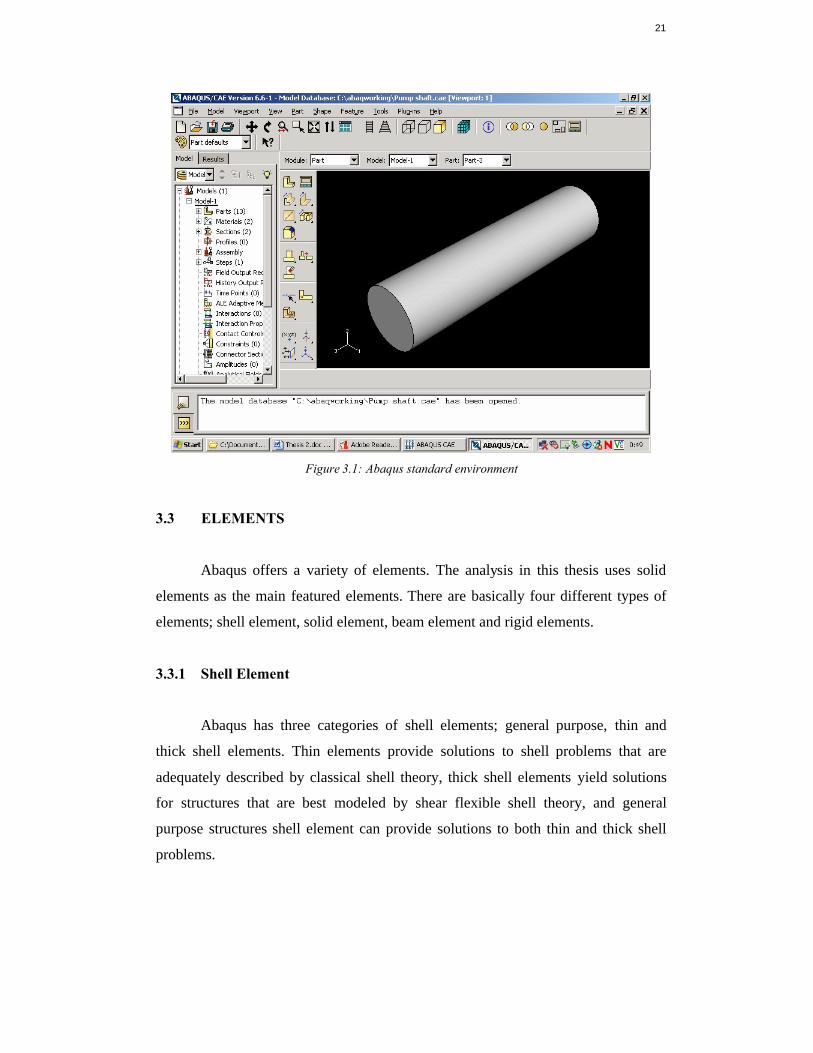
3.1 Abaqus standard environment 21

3.2 Meshing with solid elements 23

4.1 Interface of Fe-safe 26

5.1 Sectional view of pump shaft 34

5.2 Loadings on the pump shaft 35

5.3 Static analysis of pump shaft 41

6.1 3D model & boundary condition on a shaft 47

6.2 Types of loading on a shaft 48

6.3 Lateral loads applied on a shaft 49

6.4 Tangential load applied on a shaft 51

6.5 Combined loading applied on a shaft 52

6.6 Finite Element Meshing of shaft 53

6.7 Input loadings on shaft for FE-Safe 54

7.1 Distribution of Von Mises stress due to lateral load 56

7.2 High stress concentration area due to lateral load 57

7.3 Distribution of Von Mises stress due to tangential load 58

xiv

7.4 High stress concentration area due to tangential load 58

7.5 Distribution of Von Mises stress due to combined load 59

7.6 High stress concentration area due to combined load 59

7.7 Localized high stress concentration at edge of keyway 60

7.8 Distribution of fatigue life cycles of the shaft 61

7.9 Distribution of fatigue life cycle at critical area of shaft 61

7.10 Typical contour on shaft due to bending fatigue failure 62

7.11 Actual contour on the failed shaft 62

7.12 Actual failure on the pump shaft 63

7.13 Shaft broken at high stress concentration area, edge of key 63

7.14 Operational position of the shaft is horizontal 64

xv

LIST OF SYMBOLS

D, d - diameter

F - Force

G - Gravity = 9.81 m/s

I - Moment of Inertia

l - Length

m - Mass

N - Rotational velocity

P - Pressure

Q - Volumetric flow-rate

r - Radius

T - Torque

ρ - Density

xvi

LIST OF APPENDICES

APPENDIX NO. TITLE PAGE

A Preliminary Fatigue Life Analysis 69

CHAPTER 1

INTRODUCTION

1.1 BACKGROUND STUDY

Wastewater lift stations are facilities designed to move wastewater from

lower to higher elevation through pipes. Key elements of lift stations include a

wastewater receiving well (wet-well), often equipped with a screen or grinding to

remove coarse materials, pumps and piping with associated valves , motors, a power

supply system, an equipment control & alarm system, an odor control system and

ventilation system.

Lift station Equipment and systems are often installed in an enclosed

structure. They can be constructed on-site (custom-designed) or prefabricated. Lift

station capacities range from 76 liters per minute (20 gallons per minute) to more

than 378,500 liters per minute (100,000 gallons per minute). Pre-fabricated lift

stations generally have capacities of up to 38,000 liters per minute (10,000 gallons

per minute).

Centrifugal pumps are commonly used in lift stations. A trapped air column,

or bubbler system, that senses pressure and level is commonly used for pump station

control. Other control alternatives include electrodes placed at cut-off levels, floats,

2

mechanical clutches, and floating mercury switches. A more sophisticated control

operation involves the use of variable speed drives.

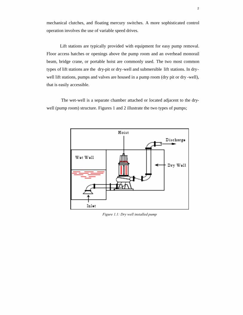
Lift stations are typically provided with equipment for easy pump removal.

Floor access hatches or openings above the pump room and an overhead monorail

beam, bridge crane, or portable hoist are commonly used. The two most common

types of lift stations are the dry-pit or dry-well and submersible lift stations. In dry-

well lift stations, pumps and valves are housed in a pump room (dry pit or dry -well),

that is easily accessible.

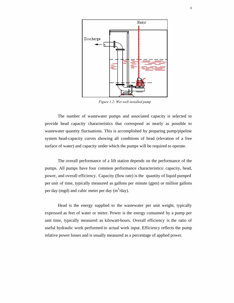
The wet-well is a separate chamber attached or located adjacent to the dry-

well (pump room) structure. Figures 1 and 2 illustrate the two types of pumps;

Figure 1.1: Dry well installed pump

3

Figure 1.2: Wet well installed pump

The number of wastewater pumps and associated capacity is selected to

provide head capacity characteristics that correspond as nearly as possible to

wastewater quantity fluctuations. This is accomplished by preparing pump/pipeline

system head-capacity curves showing all conditions of head (elevation of a free

surface of water) and capacity under which the pumps will be required to operate.

The overall performance of a lift station depends on the performance of the

pumps. All pumps have four common performance characteristics: capacity, head,

power, and overall efficiency. Capacity (flow rate) is the quantity of liquid pumped

per unit of time, typically measured as gallons per minute (gpm) or million gallons

per day (mgd) and cubic meter per day (m3/day).

Head is the energy supplied to the wastewater per unit weight, typically

expressed as feet of water or meter. Power is the energy consumed by a pump per

unit time, typically measured as kilowatt-hours. Overall efficiency is the ratio of

useful hydraulic work performed to actual work input. Efficiency reflects the pump

relative power losses and is usually measured as a percentage of applied power.

4

1.2 PROBLEM DEFINITION

Submersible pump are widely used in a wastewater pumping station and

treatment plants, to transfer sewage from a sump or wet well to other parts of the

processes. Usually when a centrifugal pump is operating at its best efficiency point

(BEP), the bending forces are evently distributed around the impeller. If the pump

discharge is throttled from this best efficiency point, then the fluid velocity is

changed and causes the hydraulic radial imbalances load to increase at the impeller

of the pump.

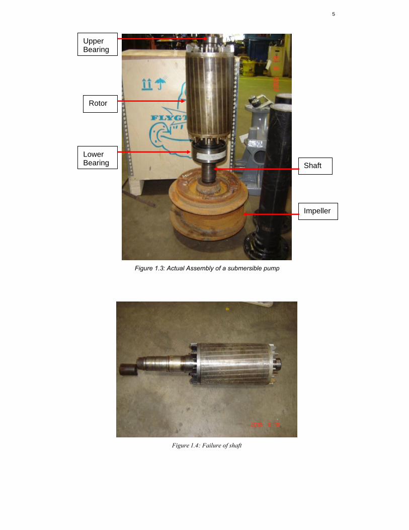
Therefore, the shaft of the submersible pump is subjected to cyclic stresses

due to this hydraulic radial imbalance loading and torsion load. It has been found

that there has been frequent failures to the shaft of the submersible pump and is

suspected due to fatigue failure caused by this cyclic stresses.

This thesis focuses mainly on the study of the distribution of stresses due to

the hydraulic radial imbalance loading, torsion load and fatigue life prediction of the

shaft parts. The analysis will be only focusing on a particular model, which has an

output of 30 KW.

5

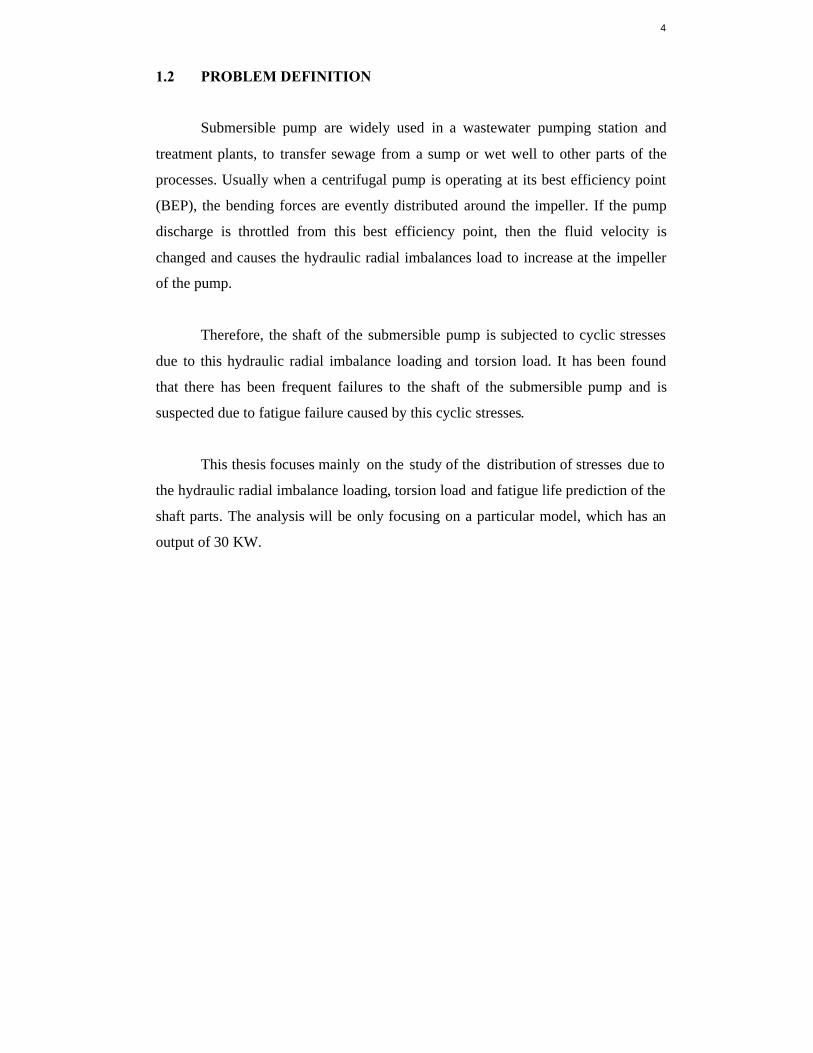
Figure 1.3: Actual Assembly of a submersible pump

Figure 1.4: Failure of shaft

Rotor

Lower Bearing

Impeller

Upper Bearing

Shaft

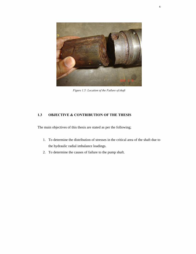
6

Figure 1.5: Location of the Failure of shaft

1.3 OBJECTIVE & CONTRIBUTION OF THE THESIS

The main objectives of this thesis are stated as per the following;

1. To determine the distribution of stresses in the critical area of the shaft due to

the hydraulic radial imbalance loadings.

2. To determine the causes of failure to the pump shaft.

7

CHAPTER 2

LITERATURE REVIEW

2.1 SHAFTS

The term "shaft" applies to rotating machine members used for transmitting

power or torque. The shaft is subject to torsion, bending, and occasionally axial

loading. Stationary and rotating members, called axles, carry rotating elements, and

are subjected primarily to bending. Transmission or line shafts are relatively long

shafts that transmit torque from motor to machine. Countershafts are short shafts

between the driver motor and the driven machine. Head shafts or stub shafts are

shafts directly connected to the motor. Motion or power can be transmitted through

an angle without gear trains, chains, or belts by using flexible shafting.

Such shafting is fabricated by building up on a single central wire one or

more superimposed layers of coiled wire. Regardless of design requirements, care

must be taken to reduce the stress concentration in notches, keyways, etc. Proper

consideration of notch sensitivity can improve the strength more significantly than

material consideration.

Equally important to the design is the proper consideration of factors known

to influence the fatigue strength of the shaft, such as surface condition, size,

temperature, residual stress, and corrosive environment. High-speed shafts require

8

not only higher shaft stiffness but also stiff bearing supports, machine housings, etc.

High-speed shafts must be carefully checked for static and dynamic unbalance and

for first-and second order critical speeds.

The design of shafts in some cases, such as those for turbo pump, is dictated

by shaft dynamics rather than by fatigue strength considerations (ref. 2). The lengths

of journals, clutches, pulleys, and hubs should be viewed critically because they very

strongly influence the overall assembly length. Pulleys, gear couplings, etc., should

be placed as close as possible to the bearing supports in order to reduce the bending

stresses.

The dimensions of shafts designed for fatigue or static strength are selected

relative to the working stress of the shaft material, the torque, the bending loads to

be sustained, and any stress concentrations or other factors influencing fatigue

strength. Shafts designed for rigidity have one or more dimensions exceeding those

determined by strength criteria in order to meet deflection requirements on axial

twist, lateral deflection, or some combination thereof. An increase in shaft diameter

may also be required to avoid unwanted critical speeds.

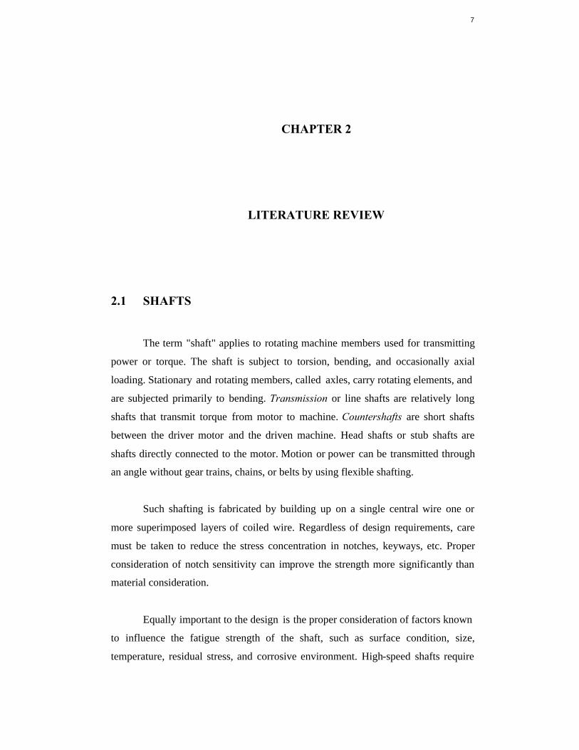
Figure 2.1: Shaft with simple bending

M M

9

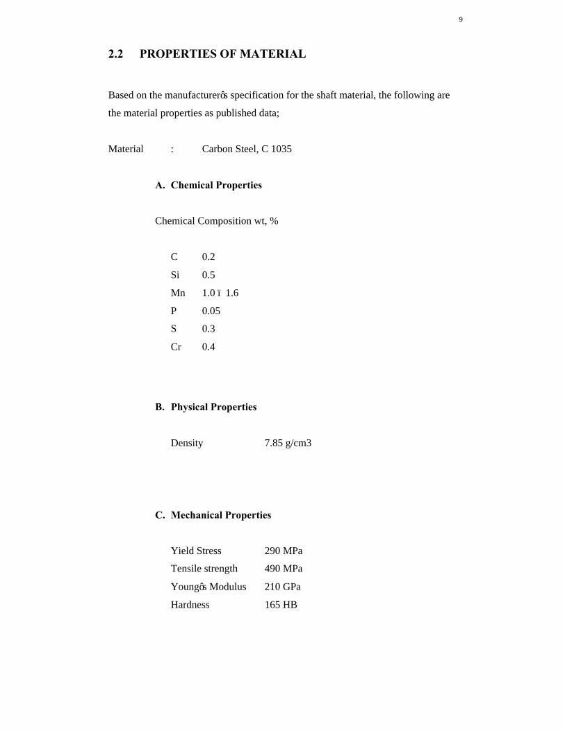
2.2 PROPERTIES OF MATERIAL

Based on the manufacturer’s specification for the shaft material, the following are

the material properties as published data;

Material : Carbon Steel, C 1035

A. Chemical Properties

Chemical Composition wt, %

C 0.2

Si 0.5

Mn 1.0 – 1.6

P 0.05

S 0.3

Cr 0.4

B. Physical Properties

Density 7.85 g/cm3

C. Mechanical Properties

Yield Stress 290 MPa

Tensile strength 490 MPa

Young’s Modulus 210 GPa

Hardness 165 HB

10

The actual shaft material has been taken and sent for chemical composition

and hardness test at Faculty of Mechanical Engineering, University Teknologi

Malaysia, to determine the actual properties of the material used, and to compare

with the properties stated as published data.

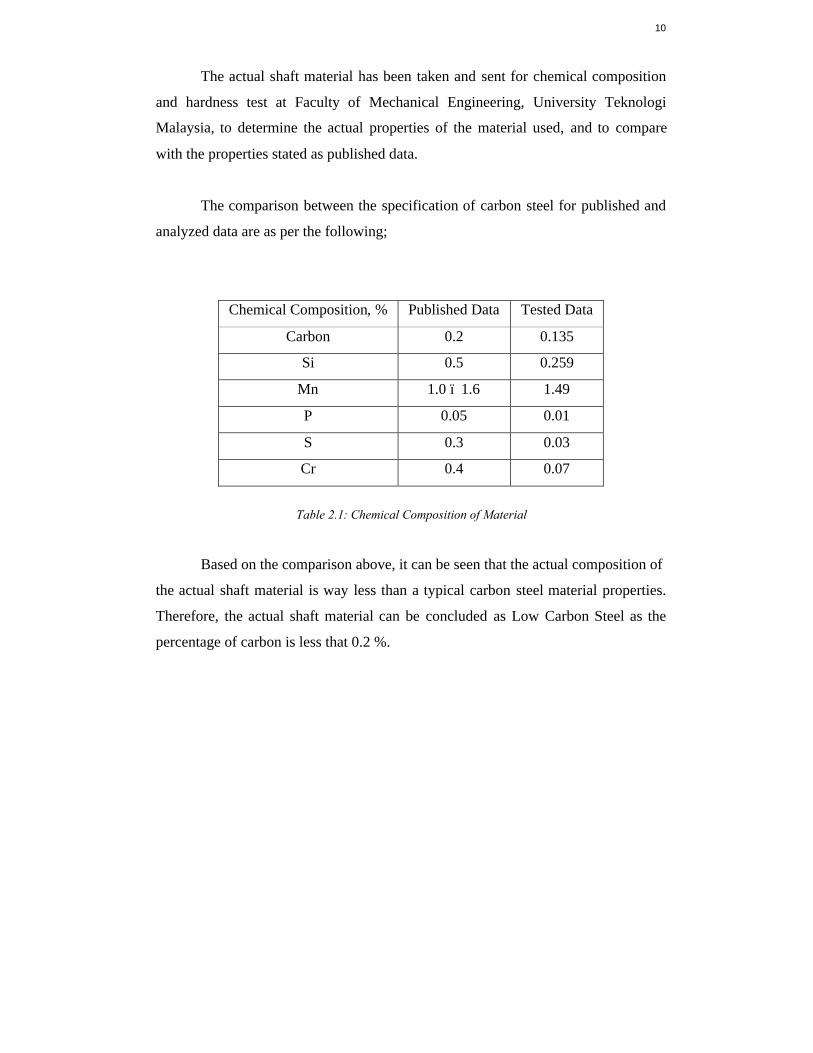
The comparison between the specification of carbon steel for published and

analyzed data are as per the following;

Chemical Composition, % Published Data Tested Data

Carbon 0.2 0.135

Si 0.5 0.259

Mn 1.0 – 1.6 1.49

P 0.05 0.01

S 0.3 0.03

Cr 0.4 0.07

Table 2.1: Chemical Composition of Material

Based on the comparison above, it can be seen that the actual composition of

the actual shaft material is way less than a typical carbon steel material properties.

Therefore, the actual shaft material can be concluded as Low Carbon Steel as the

percentage of carbon is less that 0.2 %.

11

2.3 FATIGUE

The concept of fatigue is very simple, when a motion is repeated, the object

that is doing the work becomes weak. For example, when you run, your leg and

other muscles of your body become weak, not always to the point where you can't

move them anymore, but there is a noticeable decrease in quality output.

This same principle is seen in materials. Fatigue occurs when a material is

subject to alternating stresses, over a long period of time. Examples of where

Fatigue may occur are: springs, turbine blades, airplane wings, bridges and bones.

2.3.1 Cyclic Stresses

There are three common ways in which stresses may be applied: axial,

torsional, and flexural. There are also three stress cycles with which loads may be

applied to the sample. The simplest being the reversed stress cycle . This is merely a

sine wave where the maximum stress and minimum stress differ by a negative sign.

An example of this type of stress cycle would be in an axle, where every half turn or

half period as in the case of the sine wave, the stress on a point would be reversed.

The most common type of cycle found in engineering applications is where

the maximum stress (σmax)and minimum stress ( σmin) are asymmetric (the curve is a

sine wave) not equal and opposite. This type of stress cycle is called repeated stress

cycle. A final type of cycle mode is where stress and frequency vary randomly.

12

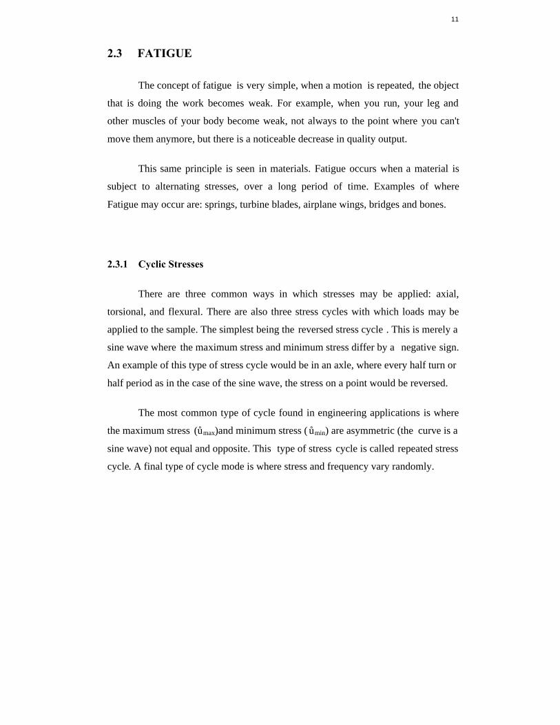
2.3.2 S-N Curve

Figure 2.2: Typical S-N Curve for a material

The significance of the fatigue limit is that if the material is loaded below

this stress, then it will not fail, regardless of the number of times it is loaded.

Material such as aluminum, copper and magnesium do not show a fatigue limit,

therefore they will fail at any stress and number of cycles.

Other important terms are fatigue strength and fatigue life. The stress at

which failure occurs for a given number of cycles is the fatigue strength. The

number of cycles required for a material to fail at a certain stress in fatigue life.

13

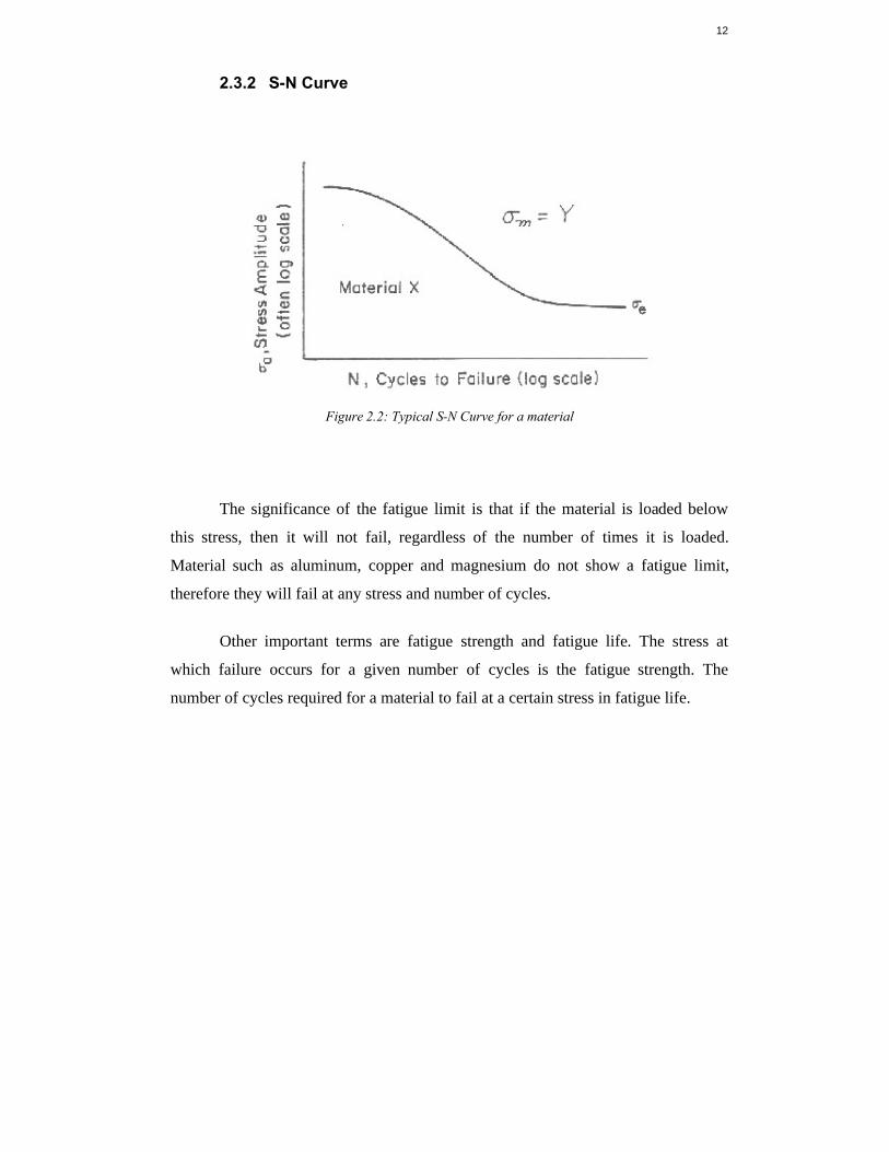
2.3.3 Crack Initiation and Propagation

Failure of a material due to fatigue may be viewed on a microscopic level in three

steps:

1. Crack Initiation: The initial crack occurs in this stage. The crack may be

caused by surface scratches caused by handling, or tooling of the material;

threads ( as in a screw or bolt); slip bands or dislocations intersecting the

surface as a result of previous cyclic loading or work hardening.

2. Crack Propagation: The crack continues to grow during this stage as a result

of continuously applied stresses

3. Failure: Failure occurs when the material that has not been affected by the

crack cannot withstand the applied stress. This stage happens very quickly.

Figure 2.3: Diagram showing location of the three steps in a fatigue fracture

under axial stress

14

2.3.4 Factors That Affect Fatigue Life and Solutions

The Mean stress has the affect that as the mean stress is increased, fatigue

life decreases. This occurs because the stress applies is greater. It is mentioned

previously that scratches and other imperfections on the surface will cause a

decrease in the life of a material. Therefore making an effort to reduce these

imperfections by reducing sharp corners, eliminating unnecessary drilling and

stamping, shot peening, and most of all careful fabrication and handling of the

material.

Another Surface treatment is called case hardening, which increases surface

hardness and fatigue life. This is achieved by exposing the component to a carbon-

rich atmosphere at high temperatures. Carbon diffuses into the material filling

interstisties and other vacancies in the material, up to 1 mm in depth.

Exposing a material to high temperatures is another cause of fatigue in

materials. Thermal expansion, and contraction will weaken bonds in a material as

well as bonds between two different materials. For example, in space shuttle heat

shield tiles, the outer covering of silicon tetraboride (SiB4) has a different coefficient

of thermal expansion than the Carbon-Carbon Composite. Upon re-entry into the

earth's atmosphere, this thermal mismatch will cause the protective covering to

weaken, and eventually fail with repeated cycles.

Another environmental affect on a material is chemical attack, or corrosion.

Small pits may form on the surface of the material, sim ilar to the effect etching has

when trying to find dislocations. This chemical attack on a material can be seen in

unprotected surface of an automobile, whether it be by road salt in the winter time or

exhaust fumes. This problem can be solved by adding protective coatings to the

material to resist chemical attack.

15

2.3.5 Causes and Recognition of Fatigue Failures

General Causes of Material Failures:

· Design deficiencies

· Manufacturing deficiencies

· Improper and insufficient maintenance

· Operational overstressing

· Environmental factors (i.e. heat, corrosion, etc.)

· Secondary stresses not considered in the normal operating conditions

· Fatigue failures

Improper and insufficient maintenance seems to be one of the most

contributing factors influenced by some improper designs such as areas that are hard

to inspect and maintain and the need for better maintenance procedures. In many

circumstances the true load is difficult to predict resulting in a structure being

stressed beyond its normal capabilities and structural limitations.

When a structure is subject to cyclic loads, areas subject to fatigue failure

must be accurately identified. This is often very hard to analyze, especially in a

highly composite structure for which analysis has a high degree of uncertainty.

Thus, in general, experimental structural fatigue testing is frequently resorted to.

Two fatigue zones are evident when investigating a fracture surface due to

fatigue, the fatigue zone and the rupture zone. The fatigue zone is the area of the

crack propagation. The area of final failure is called the rupture or instantaneous

zone. In investigation of a failed specimen, the rupture zone yields the ductility of

the material, the type of loading, and the direction of loading. The relative size of the

rupture zone compared with the fatigue zone relates the degree of overstress applied

to the structure.

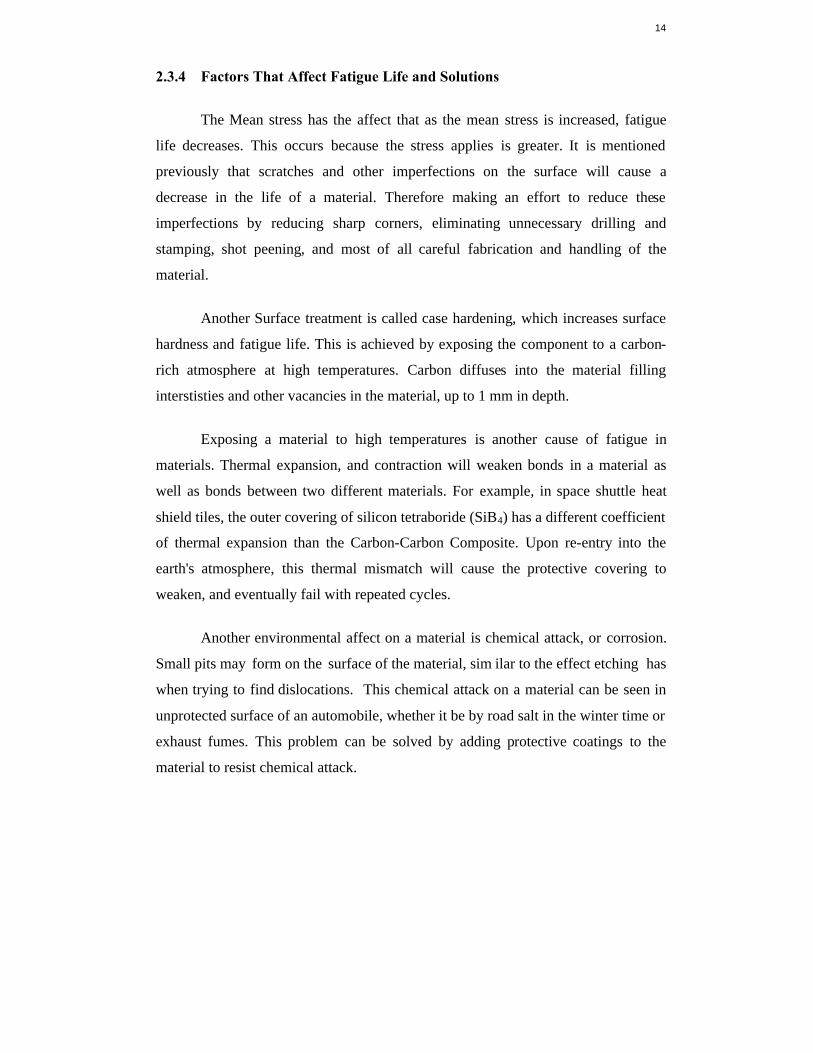
The amount of overstressing can be determined from the fatigue zone as

follows: highly overstressed if the area of the fatigue zone is very small compared

with the area of the rupture zone; medium overstress if the size or area of both zones

16

are nearly equal; low overstress if the area of rupture zone is very small. Figure 8

describe these relations between the fatigues and rupture zones.

Figure 2.4 : Fracture appearances of fatigue failures in Bending

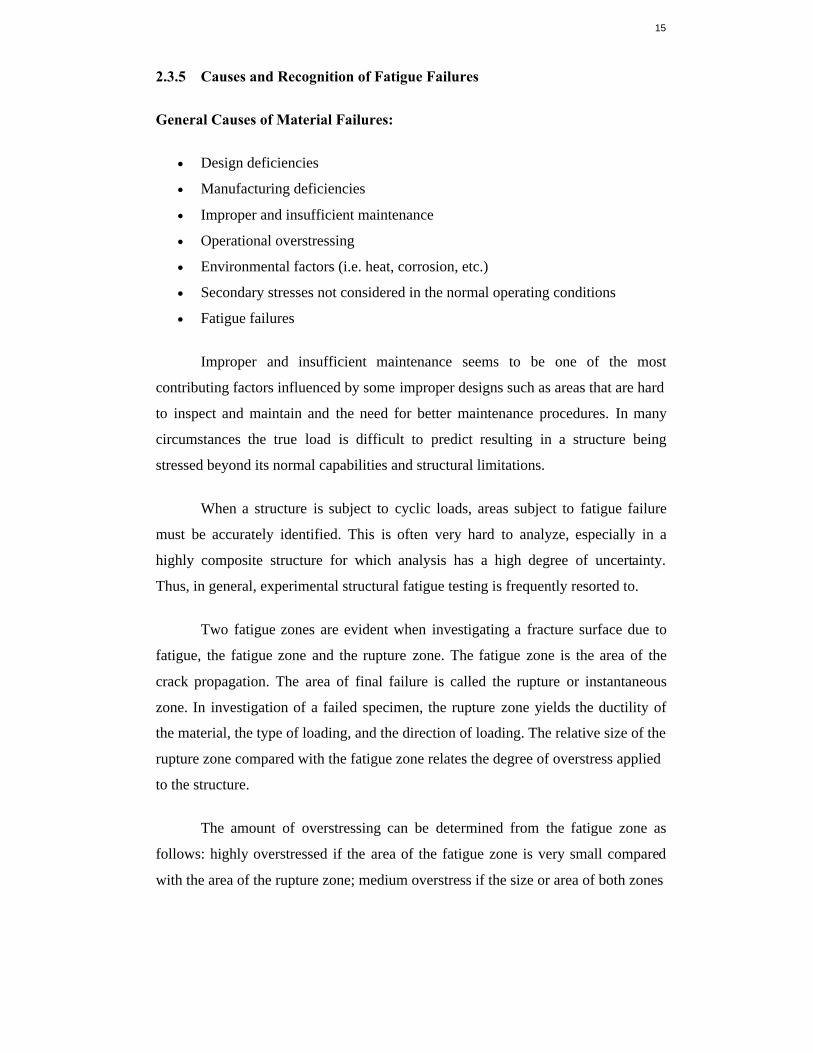
The fatigue zone can be described as follows: a smooth rubbed, and velvety

appearance, the presence of waves known as "clam-shells" or "oyster-shells", "stop

marks" and "beach marks," and the herringbone pattern or granular trace which

shows the origin of the crack. In general, stop marks indicate the variations in the

rate of crack propagation due to variations in stress amplitude in a cyclic application

varying with time.

Figure 2.5: Typical fatigue zone with identifying marks

17

2.3.6 Design Considerations

Even if careful attention to good design practices is constantly the goal of

design engineers, fatigue problems are sometimes introduced into the structure.

Fatigue failures are often the result of geometrical or strain discontinuities, poor

workmanship or improper manufacture techniques, material defects, and the

introduction of residual stresses that may add to existing service stresses.

Typical factors affecting fatigue include the following: Stres s raisers, usually

in the form of a notch or inclusion; most fatigue fractures may be attributed to notch

effects, inclusion fatigue specimens are rare. High strength materials are much more

notch-sensitive than softer alloys. Corrosion is another factor that affects fatigue.

Corroded parts form pits that act like notches. Corrosion also reduces the amount of

material which effectively reduces the strength and increases the actual stress.

Decarburization, the loss of carbon from the surface of the material, is the

next factor. Due to bending and torsion, stresses are highest at the surface;

decarburization weakens the surface by making it softer. Finally, residual stresses

which add to the design stress; the combined effect may easily exceed the limit

stress as imposed in the initial design.

2.3.7 Influence of Processing and Metallurgical Factors on Fatigue

A myriad of factors affect the behavior of a material under fatigue loading.

Obvious factors include the sign, magnitude, and frequency of loading, the geometry

and material strength level of the structure and the ambient service temperature.

However, processing and metallurgical factors are not often considered, but these

factors determine the homogeneity of materials, the sign and distribution of resi dual

stresses, and the surface finish. Thus, processing and metallurgical factors have an

overriding influence on the performance of a structure.

18

A. Processing Factors

Stresses are normally highest at the surface of a structure, so it follows that

fatigue usually initiates at the surface. Stress raisers are more likely to be present as

a result of surface irregularities introduced by the design of the structure or produced

in service or resulting from processing. Processing factors can introduce a

detrimental or beneficial effect into a structure, usually in the form of effect on

strength level or residual stress condition of the surface material. Therefore, the

effect of processing on the mechanical properties of a material, especially the

surface of the material, directly affects fatigue properties.

Processing factors that influence the fatigue life of a structure include the

following: the process by which a part is formed, such as die casting; the heat

treatment of a material, such as quenching, which builds up residual stresses and

annealing, which relieves internal stress (see Figure 3); case hardening, such as

carburization or nitriding, which increases surface hardness and strength (see Figure

4); surface finish, such as polished smooth by electro polishing; cold working, which

increases strength; also, cladding, plating, chemical conversion coatings.

B. Metallurgical Factors

Metallurgical factors refers to areas within the material, either on the surface

or in the core, which adversely affect fatig ue properties. These areas may arise from

melting practices or primary or secondary working of the material or may be

characteristic of a particular alloy system. In virtually all instances the detriment to

fatigue properties results from a local stress-raising effect.

Therefore, metallurgical factors affecting fatigue include the following:

surface defects, sub-surface and core defects, inhomogenity, anisotropy, improper

heat treatment, localized overheating, corrosion fatigue, and fretting corrosion.

19

CHAPTER 3

ABAQUS

3.1 INTRODUCTION

The Abaqus suite of software for finite element analysis consists of three

main products;

· Abaqus / Standard

· Abaqus / Explicit

· Abaqus / CAE

The standard package solves static, dynamic and thermal problems. The

explicit package focus on transient dynamics and quasi-static analysis. The CAE

package is CAD like tool to create models for analysis and for visualization of

results.

In this thesis, the models has been created in Abaqus / CAE and analysis

package used in Abaqus / Standard, hence all analysis are static.

20

3.2 CREATING MODELS

The CAE package is using different modules. These modules are used in order they

are presented so the models are created with the same procedure.

· Part Module : The parts are created using Graphical User Interface (GUI)

· Property Module: All the material properties are given such as elastic and

plastic behaviour. The orientation of the beam, etc, is given.

· Assembly Module: The parts are imported to create the geometry of the

model, i.e to build the complete structure.

· Step Module: This module decides which type of analysis that is going to be

used. The analysis is divided into one or more steps. These steps capture the

changes in the model. Here are the output requests defined. There are two

different procedures for the step;

o General – These steps define sequential events. The state of the

model at the end of one general steps.

o Linear Perturbation – These steps provide the linear response of the

model about the state reached at the end of the last general non linear

steps.

· Interaction Module: Here all the relationships between the parts defined.

· Load Module: In this module, all the loads and boundary conditions are

defined. The loads are step-dependent.

· Mesh Module: This module generates meshes on the assemblies. One part

can be divided into three different meshes and different element too.

· Job Module: The jobs are created and submitted for analysis. It is possible to

submit and write only input files for latest usage.

· Visualization Module: The results of the analysis can be visualized in this

module. It is possible to make different plots at selected.

21

Figure 3.1: Abaqus standard environment

3.3 ELEMENTS

Abaqus offers a variety of elements. The analysis in this thesis uses solid

elements as the main featured elements. There are basically four different types of

elements; shell element, solid element, beam element and rigid elements.

3.3.1 Shell Element

Abaqus has three categories of shell elements; general purpose, thin and

thick shell elements. Thin elements provide solutions to shell problems that are

adequately described by classical shell theory, thick shell elements yield solutions

for structures that are best modeled by shear flexible shell theory, and general

purpose structures shell element can provide solutions to both thin and thick shell

problems.

22

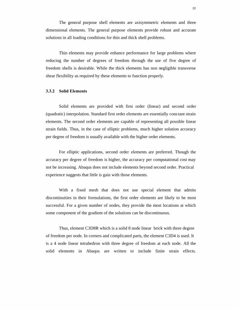
The general purpose shell elements are axisymmetric elements and three

dimensional elements. The general purpose elements provide robust and accurate

solutions in all loading conditions for thin and thick shell problems.

Thin elements may provide enhance performance for large problems where

reducing the number of degrees of freedom through the use of five degree of

freedom shells is desirable. While the thick elements has non negligible transverse

shear flexibility as required by these elements to function properly.

3.3.2 Solid Elements

Solid elements are provided with first order (linear) and second order

(quadratic) interpolation. Standard first order elements are essentially cons tant strain

elements. The second order elements are capable of representing all possible linear

strain fields. Thus, in the case of elliptic problems, much higher solution accuracy

per degree of freedom is usually available with the higher order elements.

For elliptic applications, second order elements are preferred. Though the

accuracy per degree of freedom is higher, the accuracy per computational cost may

not be increasing. Abaqus does not include elements beyond second order. Practical

experience suggests that little is gain with those elements.

With a fixed mesh that does not use special element that admits

discontinuities in their formulations, the first order elements are likely to be most

successful. For a given number of nodes, they provide the most locations at which

some component of the gradient of the solutions can be discontinuous.

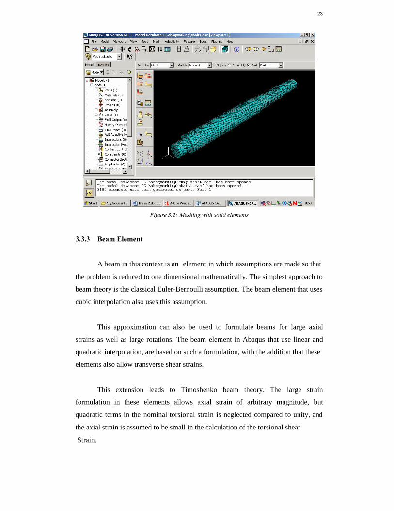
Thus, element C3D8R which is a solid 8 node linear brick with three degree

of freedom per node. In corners and complicated parts, the element C3D4 is used. It

is a 4 node linear tetrahedron with three degree of freedom at each node. All the

solid elements in Abaqus are written to include finite strain effects.

23

Figure 3.2: Meshing with solid elements

3.3.3 Beam Element

A beam in this context is an element in which assumptions are made so that

the problem is reduced to one dimensional mathematically. The simplest approach to

beam theory is the classical Euler-Bernoulli assumption. The beam element that uses

cubic interpolation also uses this assumption.

This approximation can also be used to formulate beams for large axial

strains as well as large rotations. The beam element in Abaqus that use linear and

quadratic interpolation, are based on such a formulation, with the addition that these

elements also allow transverse shear strains.

This extension leads to Timoshenko beam theory. The large strain

formulation in these elements allows axial strain of arbitrary magnitude, but

quadratic terms in the nominal torsional strain is neglected compared to unity, and

the axial strain is assumed to be small in the calculation of the torsional shear

Strain.

24

3.3.4 Rigid Elements

Rigid elements are associated with a given rigid body and share a common

node known as the rigid body reference node. A rigid element can be used t o define

the surfaces of rigid bodies for contact or to define rigid bodies for multi body

dynamic simulations. They also be attached to deformable elements or be used to

constraint parts of a model. The rigid element used is usually four node elements in

three dimensional.

25

CHAPTER 4

FE- SAFE

4.1 INTRODUCTION

FE-SAFE is an advanced easy-to-use suite of durability analysis software

which interfaces to finite element models. FE-SAFE combines component loading,

FEA stresses, and materials data, and performs advanced multiaxial fatigue analysis.

Fatigue hot-spots are automatically identified. 3-D contour plots can be displayed

for fatigue life and for allowable stress factors for a specified design life.

FE-SAFE can be used for re-design and ‘what-if’ analysis, for the whole

model or for selected areas, to investigate the effect of removing metal from non-

critical regions and to increase the life at hot-spot locations of temperature, surface

finish, notch sensitivity, geometry changes, and changes in material properties and

service duty can be investigated quickly. Designs can be optimized rapidly, material

costs are reduced, and the final design can be verified on the computer, giving more

confidence that the design will pass test schedules as right-first-time.

FE-SAFE was developed under a $1million project in collaboration with

Rover Group. Extensive tests on real components were used to develop the software.

FE-SAFE interfaces to many FEA suites and post -processors, including ABAQUS,

ANSYS, FEMSYS, IDEAS, Pro/Engineer, Pro/Mechanica, Hypermesh and FAM.

26

The ABAQUS interface reads and writes to the .fil file and the new ABAQUS/CAE

database available with ABAQUS 6.4.1.

A CATIA and a NASTRAN interface will be released later this year. FE-

SAFE is supported on Silicon Graphics, Hewlett Packard and Sun UNIX

workstations, and will be available on PC’s running Windows NT. Continuing

research projects and customer-specified developments are being used to ensure that

FE-SAFE remains at the forefront of engineering durability by design.

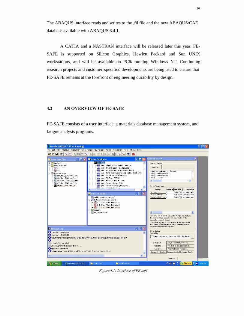
4.2 AN OVERVIEW OF FE-SAFE

FE-SAFE consists of a user interface, a materials database management system, and

fatigue analysis programs.

Figure 4.1: Interface of FE-safe

27

4.2.1 FEA stresses

· Are usually elastic stresses, so that the results can be scaled and

superimposed to

produce service stress time histories.

· Elastic-plastic stresses can be analyzed for certain types of loading.

4.2.2 Component loading

· A time history of component load can be applied to a set of FEA stresses.

· Time histories of multi-axis loading can be superimposed to produce a time

history of the stress tensor at each location on the model.

· A sequence of FEA stresses – for example, the results of a transient analysis,

or the analysis of several rotations of an engine crankshaft, or models of

several discrete loading conditions, can be analyzed.

· A combination of the above 2 items.

· Block loading programs, consisting of blocks of constant amplitude cycles,

can be produced and analyzed.

4.2.3 Materials data

· A comprehensive data base of materials properties is provided.

· The database can be extended and modified by the customer.

· Test reports and background data can be accessed using in-built Netscape

links.

· The database is accessed by FE -SAFE during the fatigue analysis set-up and

materials data is transferred into the analysis programs. The database may

also be accessed directly through the FE-SAFE user interface, to enter new

data for example.

28

4.2.4 Additional factors

· Nodal temperatures can be used to modify materials fatigue properties.

· Effects of surface finish can be included for all or part of the component

allowing machined and as-forged surfaces to be differentiated.

· Notch sensitivity effects can be included – important for cast irons, and some

aluminium alloys and lower strength steels (in Release 3.1).

· A design life may be specified.

· The fatigue analysis can be for the complete model, or for an element group.

· Different materials data or stress concentration factors can be used for each

element group (to allow for machined and as-forged surfaces on the same

component, for example)

4.2.5 Analysis

· Uniaxial analysis using stress-life curves - Goodman, Gerber or no mean

stress correction.

· Uniaxial analysis using strain-life curves – Morrow, Smith-Watson-Topper

or no mean stress correction.

· Biaxial fatigue analysis using local stress-strain analysis (maximum shear

strain, maximum direct strain, Brown-Miller combined shear and normal

strain) implemented as critical plane procedures.

· Von Mises stress.

· Analysis of welded structures using the stress-life data from BS7608.

4.2.6 Output

· FE-SAFE writes output files of nodal fatigue lives. If a design life has been

specified, FE-SAFE calculates the stress factor which could be applied at

each node to achieve this life. Both of these files can be displayed as 3-D

contour plots.

· A list of the most damaged elements is saved, and re-analysis can be

concentrated on these elements if required.

29

· A text file of user inputs, analysis type, program version numbers and a

results summary, is produced.

4.2.7 Re-analysis

· The user may change any of the inputs and re-run the analysis.

· FE-SAFE reloads all the previous input parameters when the program is re-

run.

4.2.8 Utilities

· Plots of materials data and load histories.

· Importing ASCII and other standard format data files.

· Preparation of single and multi-channel load histories – scaling, peak/valley

with cycle omission.

4.3 FATIGUE ANALYSIS ALGORITHM

The following fatigue damage algorithms are included.

Uniaxial stress – life

Δσ / 2 = σ’f (2 Nf )b

Strain life for Uniaxial stress

Δε/ 2 = (σ’f / E )(2 N1 )b + ε’f (2 Nf )c

Direct strain

Δε1/ 2 = (σ’f / E )(2 Nf )b + ε’f (2 Nf )c

30

Von Mises Strain

Δεeff/ 2 = (σ’f / E )(2 Nf )b + ε’f (2 Nf )c

4.4 A SINGLE LOAD HISTORY ON A COMPONENT

The FEA file would be an elastic analysis for a unit load. FE -SAFE allows a

scale factor to be applied to the loading if the FEA stresses are for a non-unit load.

For each node, FE-SAFE calculates a time history of the 6-stress tensor by

multiplying the unit load stress tensor by the time history of the load.

If the load case for the FE data set is a load PFE , and for this load the elastic

stress at the node is SFE . If the loading to be analysed is a load time-history P(t),

and one data point in P(t) is a value PK then the elastic stress at the node SK = SFE

A time history of the principal stresses in the plane of the element is

calculated. The multiaxial Neuber’s rule is used to calculate the elastic-plastic

stresses and strains which result from any cyclic yielding, using a material memory

algorithm. The cyclic stress-strain curve is calculated for the biaxial stress condition

at the node. If the user has specified an additional stress concentration factor, its

effect is included at this stage.

For a single load history the principal stresses at the node do not change

direction, so a single fatigue analysis is performed. In this, the shear or direct strains

are rainflow cycle counted and the fatigue damage for each cycle is calculated.

Miner’s rule is used to calculate the fatigue life at the node.

If a design life has been specified, the program uses an iteration procedure to

calculate the factor which could be applied to the stresses in order to achieve the

design life.

31

4.5 MULTIPLE LOAD DIRECTIONS ON A COMPONENT

For each loading direction, the FEA file would contain the results of an

elastic analysis for a unit load. FE-SAFE takes the 6 -stress tensor for one unit load,

and multiplies it by the time history of this load. FE-SAFE then takes the 6-stress

tensor for the second unit load, multiplies it by the time history of this load to form a

time history of the stress tensor, and adds the time history obtained from the first

load.

This is repeated for each load, to create a ti me history of the stress tensor for

all the loads or a stress data set, each of the elastic stresses at the node will be given

by an equation of the form

S = (SFE)P(P/PFE) + (SFE)Q(Q/QFE)

Where, S - Instantaneous value of one six stresses

PFE - Load used for FE Data set

SFE - Elastic stress at the node for load PFE

P - Instantaneous value of rod P(t) in load time history

QFE - Load used for 2nd FE Data set

Q - Instantaneous value of load Q(t) in load time history

The multiaxial Neuber’s rule is used to calculate the elastic-plastic stresses

and strains which result from any cyclic yielding. The cyclic stress-strain curve is re-

calculated for the biaxial stress condition for each event in the stress history, using a

material memory If the user has specified an additional stress concentration factor,

its effect is included at this stage.

For multiple load directions, the principal stresses at the node may change

direction during the load history, so a critical plane fatigue analysis is performed. On

each plane, the shear or direct strains are rainflow cycle counted and the fatigue

damage for each cycle is calculated. Miner’s rule is used to calculate the fatigue life

at the node.

32

The shortest fatigue life on any plane is taken as the fatigue life at the node.

If a design life has been specified, the program uses an iteration procedure to

calculate the factor which could be applied to the stresses in order to achieve the

design life.

4.6 DATA SET SEQUENCE

A data set sequence may be the result of a transient analysis. It may also be

created by modeling a series of discrete events, for example the stresses in an engine

crankshaft calculated at each 50 of rotation of the crankshaft through (say) four

crankshaft revolutions. The calculated stresses at each angle are termed a ‘data set’.

The data set sequence is specified in a data set sequence file, which allows the

sequence of the data sets to be specified, and allows a scale factor to be applied to

any data set.

A different scale factor may be applied to each data set (positive or

negative), and data sets may appear more than once in the sequence. At each node

FE-SAFE creates a time-history of the stress tensor from the sequence of data sets.

This is converted into elastic-plastic stress/strain and a critical plane fatigue analysis

is used to calculate the fatigue life. Again, a design life may be specified.

4.7 BLOCK LOADING ANALYSIS

Block loading fatigue tests are commonly used. FE-SAFE can simulate

block-loading sequences. The user creates a uni t load FEA data set for each load

condition. For each data set the user may specify two scale factors and a number

of cycles. For example, the stresses in data set 1 may be scaled by +1 and +0.1 to

create a stress cycle, and the user may specify 1000 cycles of this loading.

33

This forms one block in the block loading sequence. At present up to 64

blocks may be specified. Data sets may appear more than once in the sequence.

FE-SAFE calculates the fatigue damage for each block, and the fatigue damage

caused by the transition from block to block. Critical plane analysis is used.

Again, a design life may be specified.

34

CHAPTER 5

PRELIMINARY ANALYSIS OF SHAFT

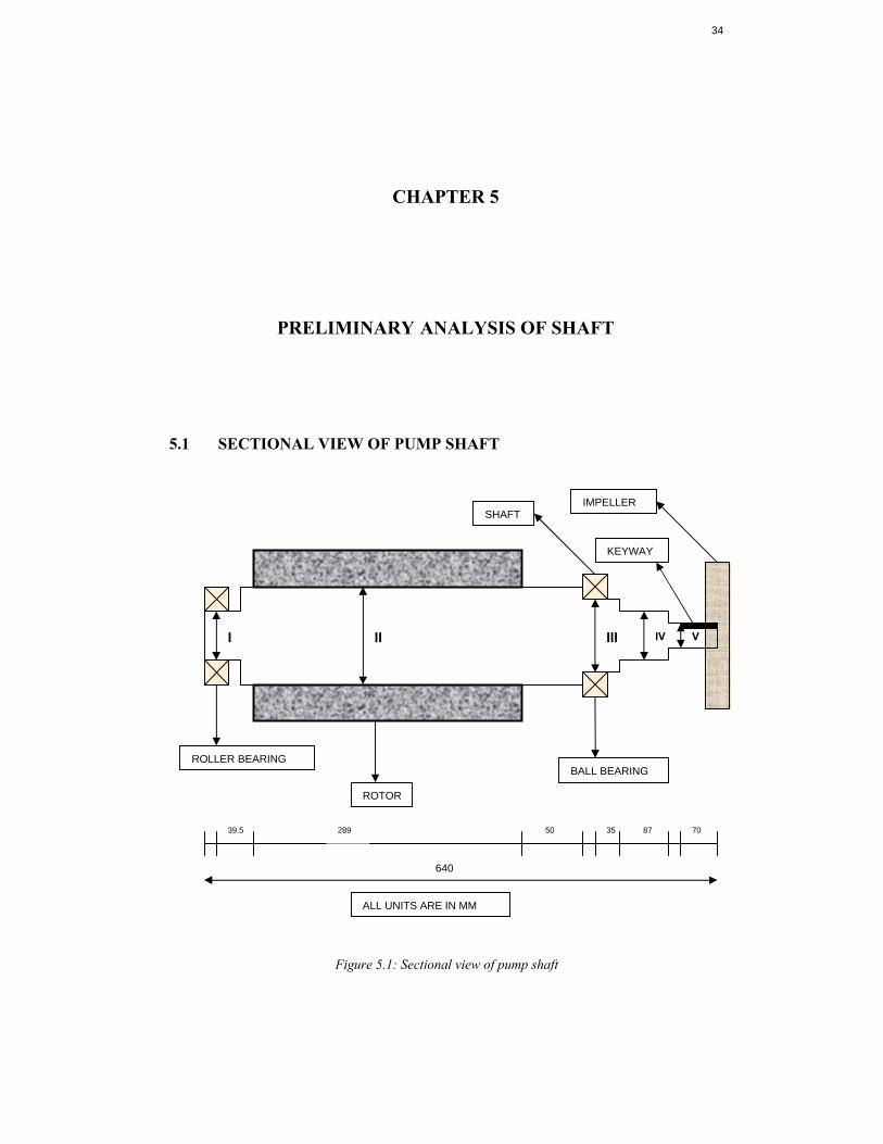
5.1 SECTIONAL VIEW OF PUMP SHAFT

Figure 5.1: Sectional view of pump shaft

III IV V II I

640

70 87 35 50 39.5

ROLLER BEARING

ROTOR

BALL BEARING

SHAFT IMPELLER

KEYWAY

289

ALL UNITS ARE IN MM

35

Diameter of shaft at various sections is as per the following;

I - 54.00 mm

II - 72.10 mm

III - 63.45 mm

IV - 57.68 mm

V - 49.03 mm

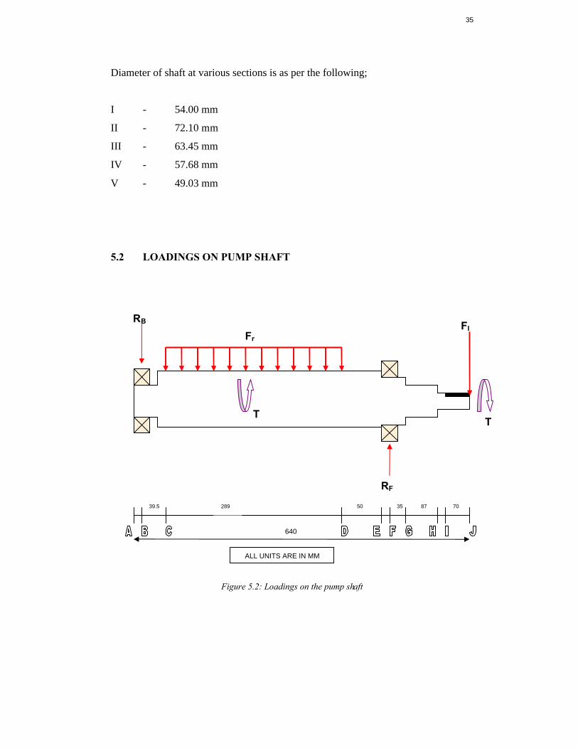
5.2 LOADINGS ON PUMP SHAFT

Figure 5.2: Loadings on the pump shaft

640

70 87 35 50 39.5 289

ALL UNITS ARE IN MM

RB Fr

FI

RF

T T

36

Where, the forces are defined as per the following;

FR = Rotor Loading

FI = Impeller Loading

RB = Reaction Load at roller bearing

RF = Reaction Load at ball bearing

T = Shaft Torque

5.3 PUMP SHAFT LOADING CALCULATIONS

5.3.1 Impeller Loading, FI

Basically, the loading at the impeller comprises of the following ;

1. Hydraulic Radial Imbalance force

2. Force due the weight of Impeller

The hydraulic radial force is Imbalance forces due to the operation of the pump

away from the best efficiency point. The amount of imbalance forces generated at

the impeller is calculated using the following formula;

P = Kq x K x H x S.G x D x B2 x 9.81

10.2

where,

K = Radial Thrust factor

S.G = Specific gravity of the pumped liquid

H = Total head at BEP (m)

B2 = Width of impeller including shrouds (cm)

D = O.D of impeller (cm)

37

while Kq is defined as,

Kq = 1 – (Q2/Qn2)2

where,

Q = Actual pumping capacity (m3/hr)

Qn = BEP pumping capacity (m3/hr)

Therefore,

K = 0.25 ( given for closed impeller )

S.G = 0.72 ( for sewage application )

H = 27.6 m ( taken from the pump performance curve )

B2 = 7.84 cm (taken from the manufacturers specifications)

D = 30 cm (taken from the manufacturers specifications)

Assumption :

Q / Qn = 0.9

Kq = 1 – (Q / Qn )4

= 1 – 0.94

= 0.344

38

Hydraulic Imbalance force becomes,

Fimb= P = Kq x K x H x S.G x D x B2 x 9.81

10.2

= 0.344 x 0.25 x 27.6 x 0.72 x 30 x 7.84 x 9.81

10.2

= 386.59 N

Load due to the weight of the impeller is given by;

Moment Inertia of Impeller = 0.38 kgm2

Diameter of impeller = 300 mm

Area, A = πd2 /4

= (3.142 x 0.32)/4

= 0.070695 m2

Therefore, weight of impeller = I / A

= 0.38 / 0.070695

= 5.38 kg

Load due to weight of impeller = mg

= 5.38 x 9.81

= 52.78 N

Impeller Loading, FI = Fimb + Fweight

= 386.59 + 52.78

= 439.37 N

39

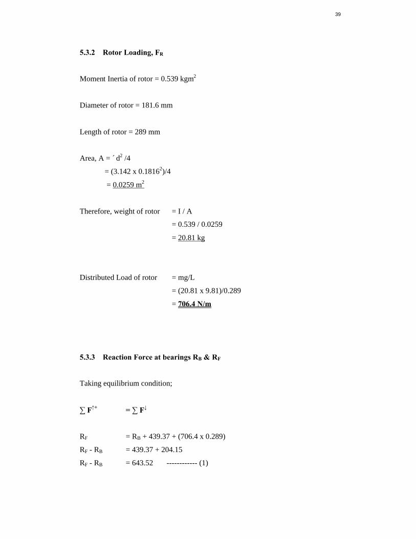
5.3.2 Rotor Loading, FR

Moment Inertia of rotor = 0.539 kgm2

Diameter of rotor = 181.6 mm

Length of rotor = 289 mm

Area, A = πd2 /4

= (3.142 x 0.18162)/4

= 0.0259 m2

Therefore, weight of rotor = I / A

= 0.539 / 0.0259

= 20.81 kg

Distributed Load of rotor = mg/L

= (20.81 x 9.81)/0.289

= 706.4 N/m

5.3.3 Reaction Force at bearings RB & RF

Taking equilibrium condition;

∑ F↑+ = ∑ F↓

RF = RB + 439.37 + (706.4 x 0.289)

RF - RB = 439.37 + 204.15

RF - RB = 643.52 ------------ (1)

40

∑ MB = 0

RF x 0.4085 = (706.4 x 0.3285 x 0.3285/2 ) – (706.4 x 0.0395 x 0.0395/2 ) +

(439.37 x 0.629)

0.4085 RF = 38.11 – 0.55 + 276.36

0.4085 RF = 313.92

RF = 313.92 / 0.4085

RF = 768.47 N

Therefore,

RF - RB = 643.52

- RB = 643.52 - RF

- RB = 643.52 – 768.47

- RB = - 124.95

RB = 124.95 N

* Shaft Torque is given by the manufacturer = 200 Nm

41

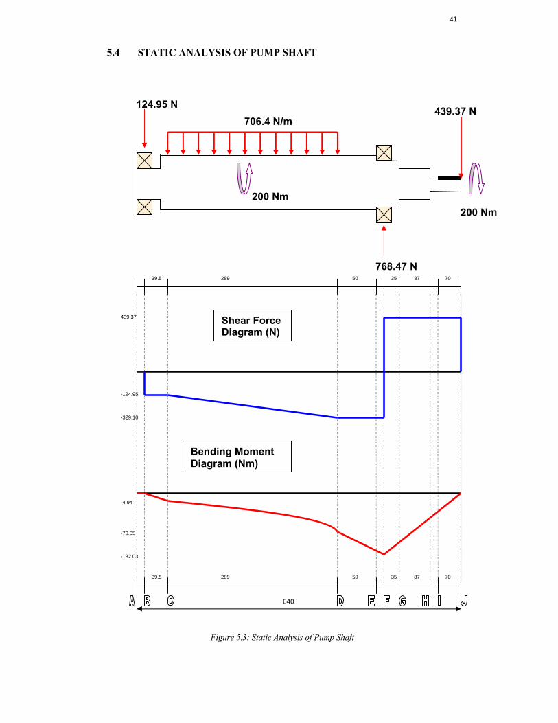
5.4 STATIC ANALYSIS OF PUMP SHAFT

Figure 5.3: Static Analysis of Pump Shaft

-132.03

-70.55

-4.94

-329.10

439.37

-124.95

289

289

70 87 35 50 39.5

124.95 N 706.4 N/m

439.37 N

768.47 N

200 Nm 200 Nm

640

70 87 35 50 39.5

Shear Force Diagram (N)

Bending Moment Diagram (Nm)

42

5.5 FATIGUE ANALYSIS OF PUMP SHAFT

The submersible pump’s shaft is made from Low Carbon steel. The designed

material properties are as below;

Young’s Modulus, E = 210 GPa

Rigidity Modulus, G = 80 GPa

Ultimate Strength, St = 490 MPa

Yield Strength, Sy = 290 MPa

Endurance limit for Mechanical element is defined as;

Se = KaKbKcKdKeSe’

Where,

Ka - Surface factor

Kb - Size factor

Kc - Load factor

Kd - Temperature factor

Ke - Fatigue strength reduction factor

Se’ - Endurance limit or fatigue limit

As for the pump shaft;

Endurance limit, is defined as Se’ = 0.504 St (for steels with St ≤ 1400 MPa )

Therefore,

Se’ = 0.504 St

= 0.504 (490)

= 246.96 MPa

43

- Surface factor, Ka = aStb

For a machined steel, the value a & b is given as ;

a = 4.51 MPa & b = -0.265 (based on table 7.4 from Shigley/Mischke : Mech. Eng. Design, 5th Edition)

Ka = aStb

= 4.51 x 490-0.265

= 0.874

- Size factor, Kb is given as 0.60 to 0.75 for bending problems

(size larger than 51 mm in diameter).

Therefore, the size factor is assumed to be 0.75.

Kb = 0.75

- Load factor, Kc is given as 1.0 for bending problems.

Kc = 1.0

- Temperature factor, Kd is given as 1.0 for temperature up to 50oC.

Kd = 1.0

Based on the bending moment diagram, the location with suspected high stress

concentration are location F, G, H & I. therefore, the fatigue life analysis will be

carried out on these locations.

44

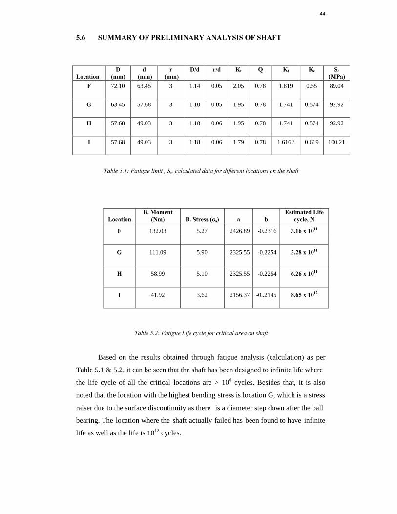
5.6 SUMMARY OF PRELIMINARY ANALYSIS OF SHAFT

Table 5.1: Fatigue limit , Se, calculated data for different locations on the shaft

Table 5.2: Fatigue Life cycle for critical area on shaft

Based on the results obtained through fatigue analysis (calculation) as per

Table 5.1 & 5.2, it can be seen that the shaft has been designed to infinite life where

the life cycle of all the critical locations are > 106 cycles. Besides that, it is also

noted that the location with the highest bending stress is location G, which is a stress

raiser due to the surface discontinuity as there is a diameter step down after the ball

bearing. The location where the shaft actually failed has been found to have infinite

life as well as the life is 1012 cycles.

Location D

(mm) d

(mm) r

(mm) D/d

r/d

Kt

Q

Kf

Ke

Se (MPa)

F 72.10 63.45 3 1.14 0.05 2.05 0.78 1.819 0.55 89.04

G 63.45 57.68 3 1.10 0.05 1.95 0.78 1.741 0.574 92.92

H 57.68 49.03 3 1.18 0.06 1.95 0.78 1.741 0.574 92.92 I 57.68 49.03 3 1.18 0.06 1.79 0.78 1.6162 0.619 100.21

Location B. Moment

(Nm) B. Stress (σa) a b Estimated Life

cycle, N

F 132.03 5.27 2426.89 -0.2316 3.16 x 1011

G 111.09 5.90 2325.55 -0.2254 3.28 x 1011

H 58.99 5.10 2325.55 -0.2254 6.26 x 1011

I 41.92 3.62 2156.37 -0..2145 8.65 x 1012

45

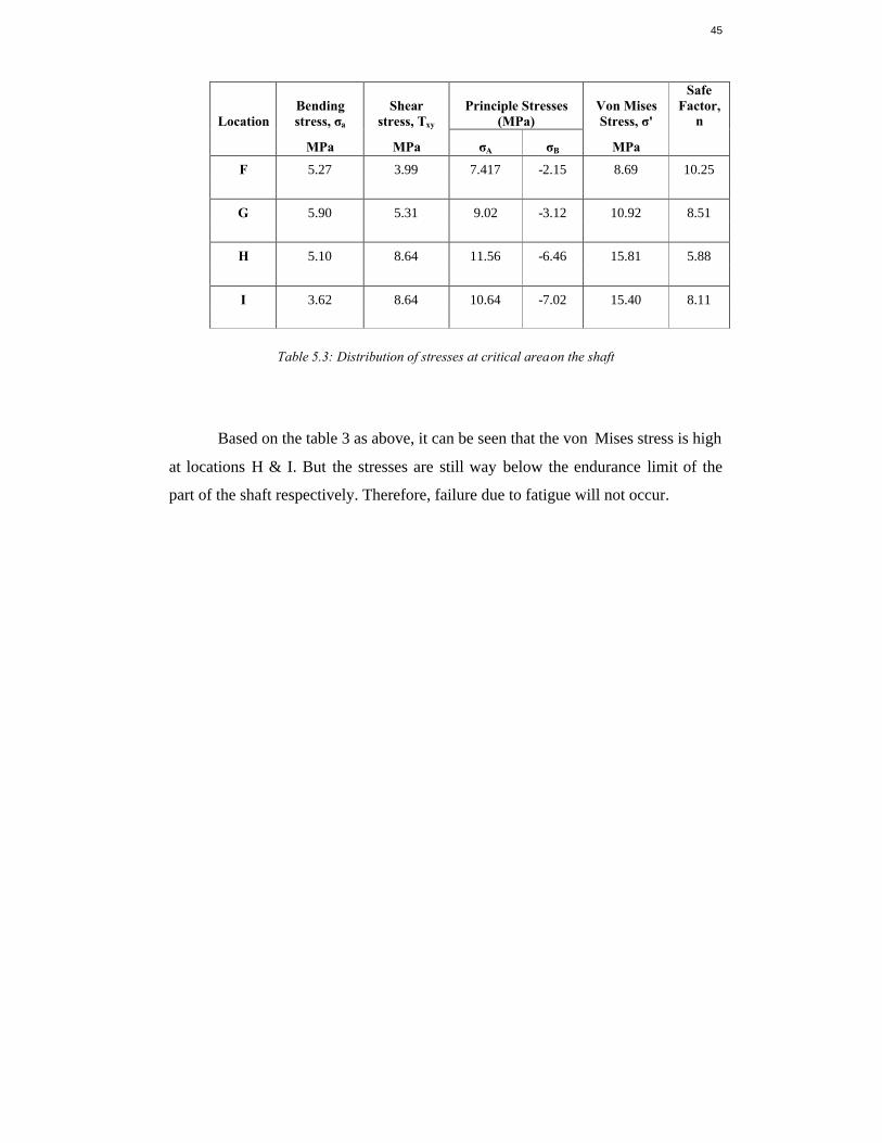
Table 5.3: Distribution of stresses at critical area on the shaft

Based on the table 3 as above, it can be seen that the von Mises stress is high

at locations H & I. But the stresses are still way below the endurance limit of the

part of the shaft respectively. Therefore, failure due to fatigue will not occur.

Location Bending stress, σa

Shear stress, Txy

Principle Stresses (MPa)

Von Mises Stress, σ'

Safe Factor,

n

MPa MPa σA σB MPa F 5.27 3.99 7.417 -2.15 8.69 10.25

G 5.90 5.31 9.02 -3.12 10.92 8.51 H 5.10 8.64 11.56 -6.46 15.81 5.88 I 3.62 8.64 10.64 -7.02 15.40 8.11

46

CHAPTER 6

3-D SHAFT ANALYSIS

6.1 FINITE ELEMENT ANALYSIS

6.1.1 Modeling of shaft

The submersible pump shaft was m odeled using existing commercial

FEA software, ABAQUS. The dimensions or size of the shaft modeled was

to the exact dimensions of the shaft that has failed in practical use.

There are two (2) boundary conditions for the shaft, which is at the

location where the shafts are supported by its upper and lower bearings. The

details of the boundary conditions are as follows;

Boundary Condition 1 : Upper bearing (Thrust bearing)

U1 = 0, U2 = 0, U3 = 0

UR1 = 0, UR2 = 0

Boundary Condition 2 : Lower bearing (Ball bearing)

U1 = 0, U2 = 0, U3 = 0

UR1 = 0, UR2 = 0

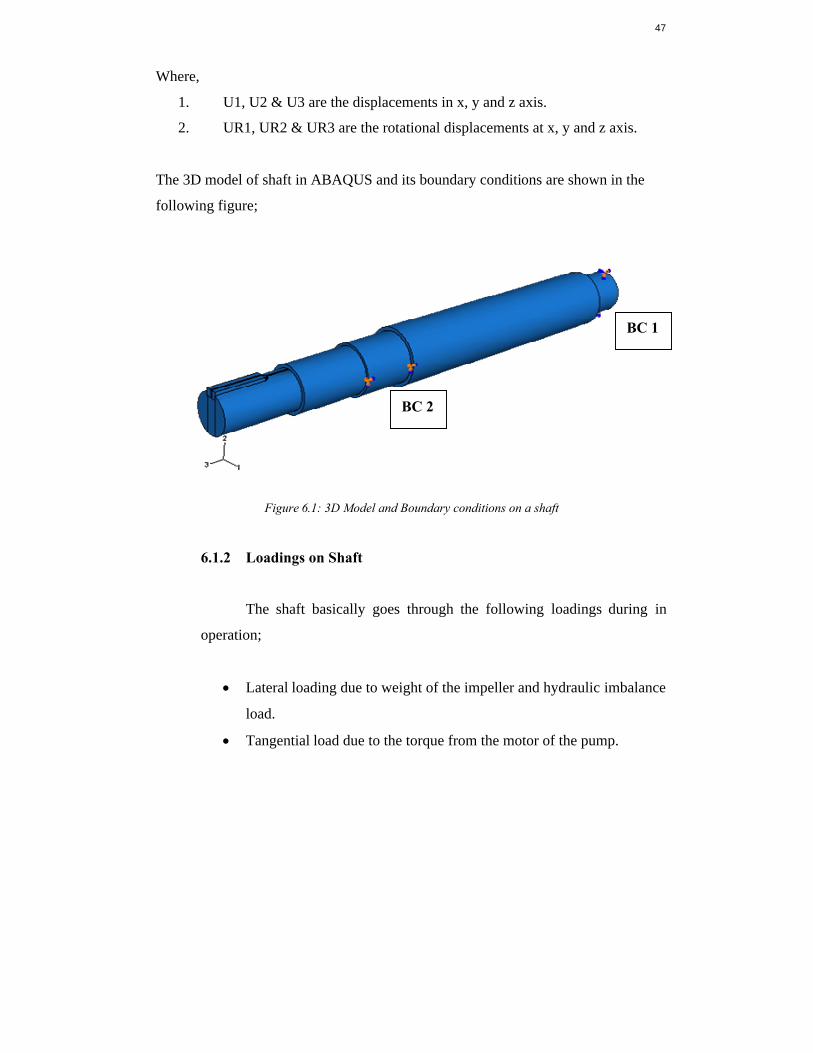
47

Where,

1. U1, U2 & U3 are the displacements in x, y and z axis.

2. UR1, UR2 & UR3 are the rotational displacements at x, y and z axis.

The 3D model of shaft in ABAQUS and its boundary conditions are shown in the

following figure;

Figure 6.1: 3D Model and Boundary conditions on a shaft

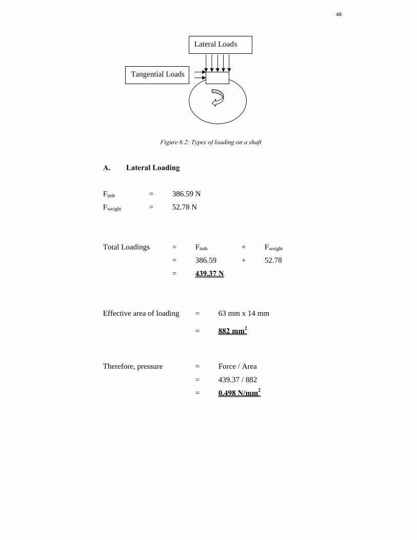
6.1.2 Loadings on Shaft

The shaft basically goes through the following loadings during in

operation;

· Lateral loading due to weight of the impeller and hydraulic imbalance

load.

· Tangential load due to the torque from the motor of the pump.

BC 2

BC 1

48

Figure 6.2: Types of loading on a shaft

A. Lateral Loading

Fimb = 386.59 N

Fweight = 52.78 N

Total Loadings = Fimb + Fweight

= 386.59 + 52.78

= 439.37 N

Effective area of loading = 63 mm x 14 mm = 882 mm2

Therefore, pressure = Force / Area

= 439.37 / 882

= 0.498 N/mm2

Lateral Loads

Tangential Loads

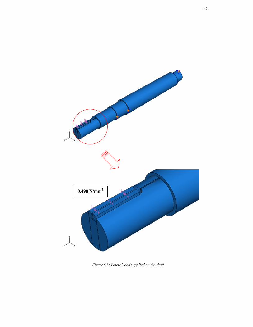
49

Figure 6.3: Lateral loads applied on the shaft

0.498 N/mm2

50

B. Tangential Loading

The following are the technical data specified by the manufacturer of the

pump;

Power of pump, P = 30 KW

RPM, N = 1455

Therefore;

Torque, T = (60 x Power )/ (2 x 3.142 x N)

= (60 x 30000000) / (2 x 3.142 x1455) = 196.89 KN/mm

Tangential load = T / r

= 196.89 / 24.5

= 8,036.44 N

So, the pressure due to the torsional loading;

Pressure = F / A = 8,036.44 / (63 x 4.5) = 28.35 N/mm2

51

Figure 6.4: Tangential load applied on the shaft

28.35 N/mm2

52

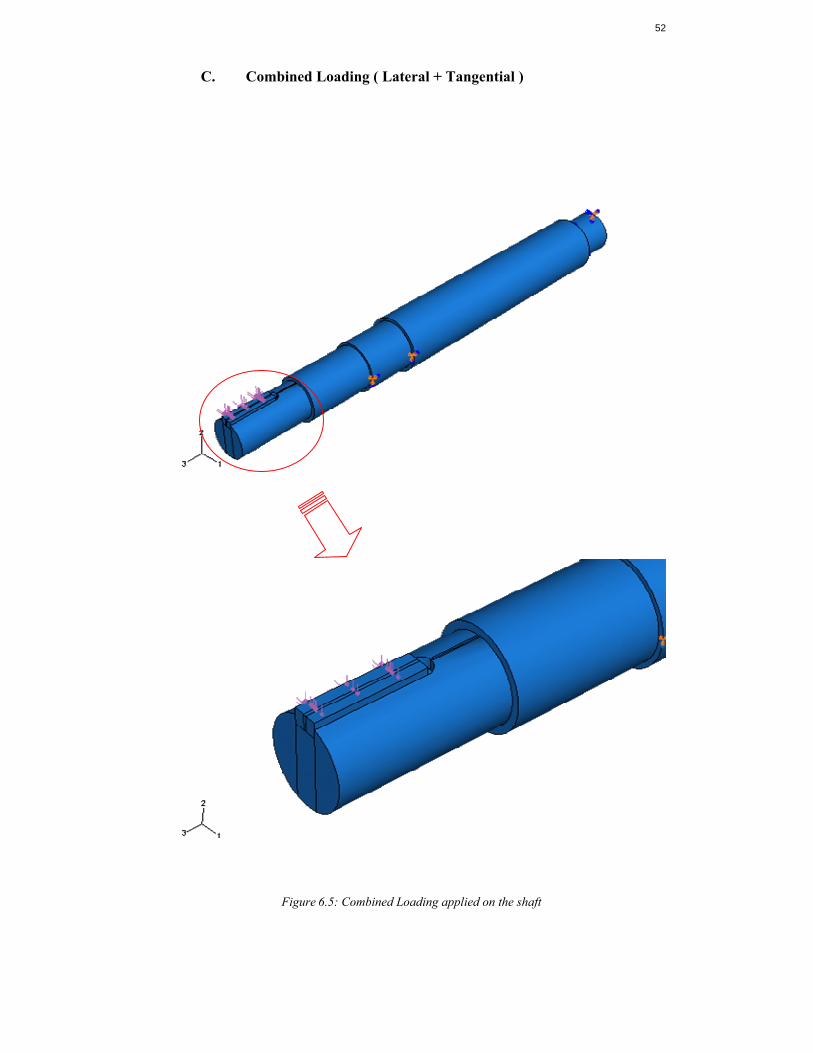
C. Combined Loading ( Lateral + Tangential )

Figure 6.5: Combined Loading applied on the shaft

53

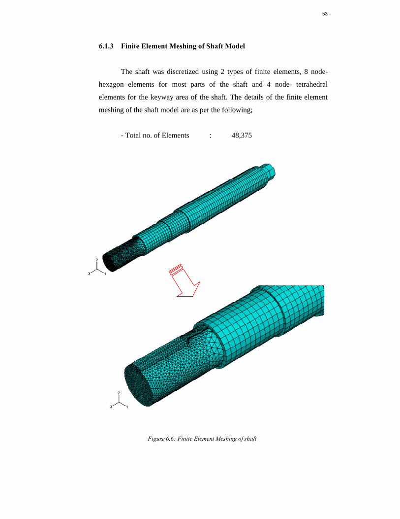
6.1.3 Finite Element Meshing of Shaft Model

The shaft was discretized using 2 types of finite elements, 8 node-

hexagon elements for most parts of the shaft and 4 node- tetrahedral

elements for the keyway area of the shaft. The details of the finite element

meshing of the shaft model are as per the following;

- Total no. of Elements : 48,375

Figure 6.6: Finite Element Meshing of shaft

54

6.2 FATIGUE LIFE ANALYSIS

6.2.1 Modeling of shaft

The input models for the Fe-safe is imported from the same .cae and

.odb file generated previously in ABAQUS. Therefore, the boundary

conditions remain unchanged from the previous setting or position.

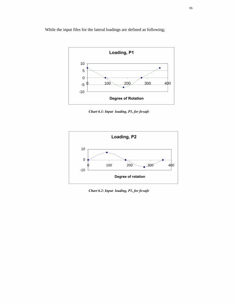
6.2.2 Loadings on Shaft

During operation, the shaft rotates while the loadings are static or the

same at the same directions. Therefore, to model the input file to Fe -safe, the

loadings are represented in way that the shaft is now in static position whil e

the loadings fluctuate over period of time.

Basically, variation of load at any point in the shaft depends on the

angular position of the shaft as it rotates. In FE -Safe, the shaft is analyzed as

a stationary component. Thus, equivalent load variation per rotation of shaft

is obtained through variable loading as illustrated in the figure below;

Figure 6.7: Input loadings on shaft for FE Safe

Where,

P1 & P2 represents the lateral loading and P3 represents the tangential load.

P1

P2 ω

P3

55

While the input files for the lateral loadings are defined as following;

Chart 6.1: Input loading, P1, for fe-safe

Chart 6.2: Input loading, P1, for fe-safe

Loading, P1

-10

-5

0

5

10

0 100 200 300 400

Degree of Rotation

Load, N

Loading, P2

-10

0

10

0 100 200 300 400

Degree of rotation

Load, N

56

CHAPTER 7

RESULTS AND DISCUSSION

7.1 FINITE ELEMENT ANALYSIS

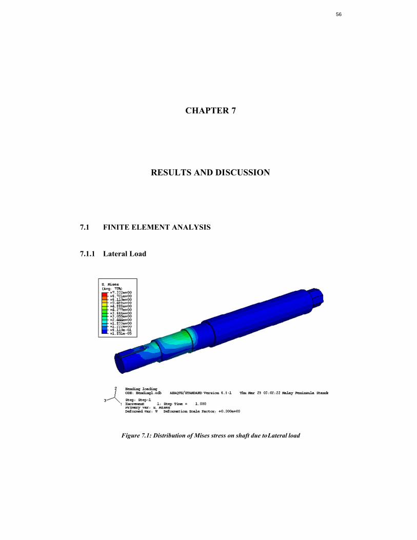
7.1.1 Lateral Load

Figure 7.1: Distribution of Mises stress on shaft due to Lateral load

57

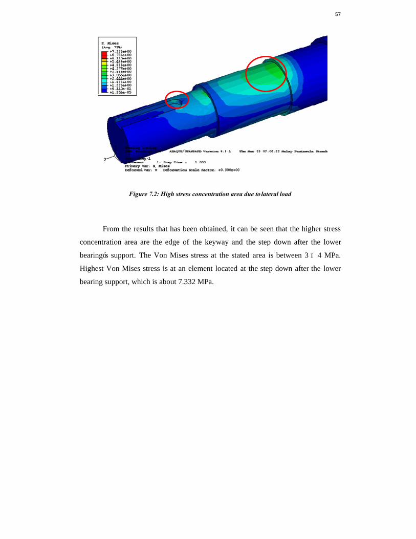
Figure 7.2: High stress concentration area due to lateral load

From the results that has been obtained, it can be seen that the higher stress

concentration area are the edge of the keyway and the step down after the lower

bearing‘s support. The Von Mises stress at the stated area is between 3 – 4 MPa.

Highest Von Mises stress is at an element located at the step down after the lower

bearing support, which is about 7.332 MPa.

58

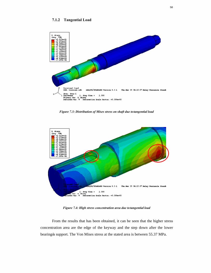
7.1.2 Tangential Load

Figure 7.3: Distribution of Mises stress on shaft due to tangential load

Figure 7.4: High stress concentration area due to tangential load

From the results that has been obtained, it can be seen that the higher stress

concentration area are the edge of the keyway and the step down after the lower

bearing‘s support. The Von Mises stress at the stated area is between 55.37 MPa.

59

7.1.3 Combined Loading (Lateral & Tangential)

Figure 7.5: Distribution of Mises stress on shaft due to combined load

Figure 7.6: High stress concentration area due to combined load

60

Figure 7.7: Localized high stress concentration at edge of keyway

From the results that had been obtained, it can be seen that the higher stress

concentration area are still the same location but the value of von Mises stress has

increased. It shows that the high stress region are very localized and the Von Mises

stress at the stated area is 55.70 MPa.

61

7.2 FATIGUE LIFE ANALYSIS

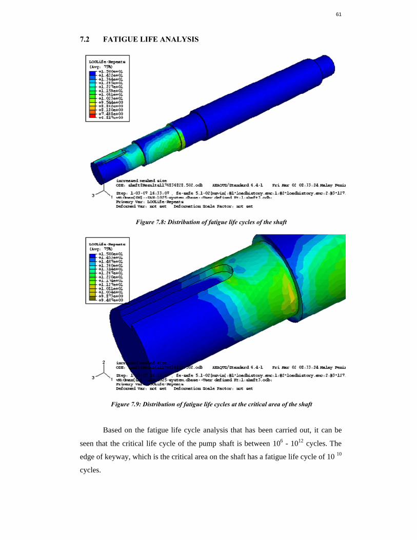
Figure 7.8: Distribution of fatigue life cycles of the shaft

Figure 7.9: Distribution of fatigue life cycles at the critical area of the shaft

Based on the fatigue life cycle analysis that has been carried out, it can be

seen that the critical life cycle of the pump shaft is between 106 - 1012 cycles. The

edge of keyway, which is the critical area on the shaft has a fatigue life cycle of 10 10

cycles.

62

7.3 VISUAL INSPECTION

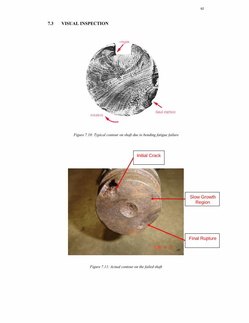
Figure 7.10: Typical contour on shaft due to bending fatigue failure

Figure 7.11: Actual contour on the failed shaft

Initial Crack

Slow Growth Region

Final Rupture

63

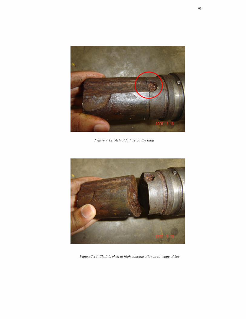
Figure 7.12: Actual failure on the shaft

Figure 7.13: Shaft broken at high concentration area; edge of key

64

Based on the visual inspection or analysis on the actual failed pump shaft, it

can be seen that the failure contour is similar to a bending fatigue failure contour

with initial crack, slow growth region and final rupture of the shaft. The shaft

actually fails at the high stress concentration region; where the edge of the key is

seated on the keyway of the shaft.

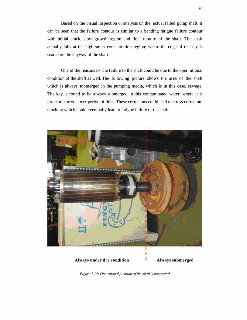
One of the reasons to the failure to the shaft could be due to the oper ational

condition of the shaft as well. The following picture shows the area of the shaft

which is always submerged in the pumping media, which is in this case, sewage.

The key is found to be always submerged in this contaminated water, where it is

prune to corrode over period of time. These corrosions could lead to stress corrosion

cracking which could eventually lead to fatigue failure of the shaft.

Always under dry condition Always submerged

Figure 7.14: Operational position of the shaft is horizontal

65

CHAPTER 8

CONCLUSION

Based on the finite element analysis that has been carried out, it can be

concluded that the material of the shaft has not yielded as the Von Mises stress

obtained is only 55.70 MPa, which is very much less than the yield stress of the

material which is 290 MPa. But the FEA analysis has given us an indication that the

stress concentration at the edge of the keyway is very high compared to the other

areas on the shaft.

After conducting the fatigue life cycle analysis on the shaft, we can

acknowledge that the fatigue life cycle of the critical area on shaft is between 10 6 to

1012 cycles and the life cycle at the edge of the keyway is about 1012 cycles. This

shows that the shaft has been designed not to fail due to fatigue.

But the results from the visual inspection of the failed shaft are actually

showing similar surface contour with a typical contour of fatigue failure. This could

be due to stress corrosion factor. The shaft keyway is always submerged in water,

which in this application is sewage water (dirty, contaminated, etc). Therefore, there

is a high possibility of corrosion to incur in which eventually causes stress corrosion

initial cracks at high stress concentration area such as the edge of key on the

keyway.

66

Other causes to the failure of the shaft could be pitting due to corrosion and

cavitations during operation of the pump. This is because pitting could cause stress

raisers on the shaft which eventually leads to fatigue failure. Besides that, a defect

on the surface of the shaft during manufacturing processes could also lead to initial

cracks to occur when the shaft is in operation. This imperfection on the surface

finish creates high stress concentration zone where the cracks develops during

operation of the shaft over period of time.

Since the shaft has been designed for infinite life, these other factors are

suspected to be the main contributors to the failure of the shaft, mainly due to

fatigue under cyclic loading when it is in operation.

67

REFERENCES

1. Joseph E. Shigley Charles R. Mischke. Mechanical Engineering Design, 5th

Edition: McGraw Hill International Edition; 1989.

2. Austin H.Bounett. The cause and Analysis of Bearing and Shaft Failures:

EASA Technical Note; 1999.

3. ITT Industries (Flygt). Shaft and Bearing Calculations; 2004.

4. ITT Industries (Flygt). Materials; 2000.

5. Dr. Andrei Lozzi. Shafts and Axles: School of Aerospace, Mechanical and

Mechatronic Engineering; 2006.

6. Noah N. Mauring. Designing the shaft diameter for acceptable level of stress:

Journal of Mechanical Design; 2000.

7. R.E Peterson. Stress Concentration Factors; 1974.

8. G.L Huyett. Engineering Handbook; 2004.

9. Stuart H. Loewenthal. Design of power transmitting shaft: NASA

Publications 1123; 1984.

10. Bruno Conegliano. Sewers – Lifting Station: Environmental Publisher

Association; 2000.

11. ITT Industries (Flygt): Technical Specifications C3201; 2000.

12. Arthur Marczewski. Numerical Fatigue Analysis of cracked rotor; 2004.

13. K. Holmedahl. Prediction of High Cycle Fatigue; 1999.

14. Dr. Robert Adey. Fatigue Life & crack growth prediction; 2004.

15. Dr. Joe Evans. Sewage pump impeller selection; 2000.

16. Dr. Jean C. Bailey. Forces on centrifugal pump impeller; 1985.

17. SEW Eurodrive. Torque Advantages: Technical note; 2006.

18. McNally. Shaft Deflection & Bending Formula; 2000.

19. Fe-safe Brochure 1/rev5: Safe Technology ltd; 1999.

68

20. Fe-safe user manual: Safe Technology ltd; 2003.

21. Abaqus user manual: ABAQUS Inc; 2001.

69

APPENDIX A

PRELIMINARY FATIGUE LIFE ANALYSIS

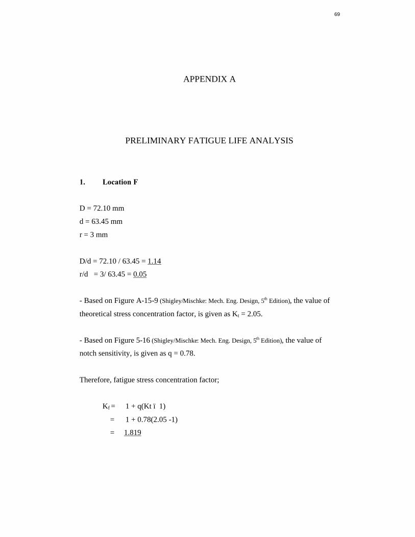
1. Location F

D = 72.10 mm

d = 63.45 mm

r = 3 mm

D/d = 72.10 / 63.45 = 1.14

r/d = 3/ 63.45 = 0.05

- Based on Figure A-15-9 (Shigley/Mischke: Mech. Eng. Design, 5th Edition), the value of

theoretical stress concentration factor, is given as Kt = 2.05.

- Based on Figure 5-16 (Shigley/Mischke: Mech. Eng. Design, 5th Edition), the value of

notch sensitivity, is given as q = 0.78.

Therefore, fatigue stress concentration factor;

Kf = 1 + q(Kt – 1)

= 1 + 0.78(2.05 -1)

= 1.819

70

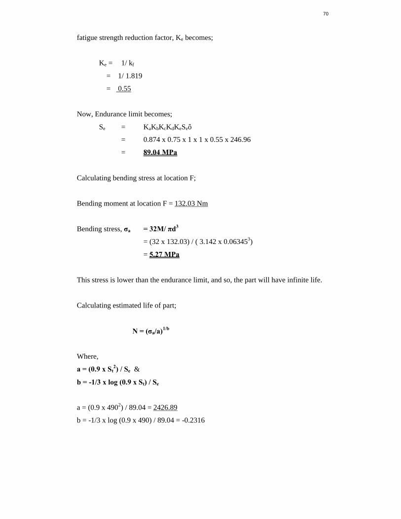
fatigue strength reduction factor, Ke becomes;

Ke = 1/ kf

= 1/ 1.819

= 0.55

Now, Endurance limit becomes;


= 0.874 x 0.75 x 1 x 1 x 0.55 x 246.96

= 89.04 MPa

Calculating bending stress at location F;

Bending moment at location F = 132.03 Nm

Bending stress, σa = 32M/ πd3

= (32 x 132.03) / ( 3.142 x 0.063453)

= 5.27 MPa

This stress is lower than the endurance limit, and so, the part will have infinite life.

Calculating estimated life of part;

N = (σa/a)1/b

Where,

a = (0.9 x St2) / Se &

b = -1/3 x log (0.9 x St) / Se

a = (0.9 x 4902) / 89.04 = 2426.89

b = -1/3 x log (0.9 x 490) / 89.04 = -0.2316

71

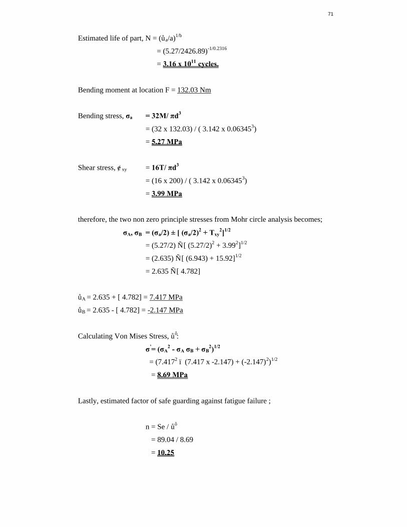
Estimated life of part, N = (σa/a)1/b

= (5.27/2426.89)-1/0.2316

= 3.16 x 1011 cycles.

Bending moment at location F = 132.03 Nm


= (32 x 132.03) / ( 3.142 x 0.063453)

= 5.27 MPa

Shear stress, Τxy = 16T/ πd3

= (16 x 200) / ( 3.142 x 0.063453)

= 3.99 MPa

therefore, the two non zero principle stresses from Mohr circle analysis becomes;

σA, σB = (σa/2) ± [ (σa/2)2 + Τxy2]1/2

= (5.27/2) ± [ (5.27/2)2 + 3.992]1/2

= (2.635) ± [ (6.943) + 15.92]1/2

= 2.635 ± [ 4.782]

σA = 2.635 + [ 4.782] = 7.417 MPa

σB = 2.635 - [ 4.782] = -2.147 MPa

Calculating Von Mises Stress, σ’:

σ’= (σA2 - σA σB + σB

2)1/2

= (7.4172 – (7.417 x -2.147) + (-2.147)2)1/2

= 8.69 MPa

Lastly, estimated factor of safe guarding against fatigue failure ;

n = Se / σ’

= 89.04 / 8.69

= 10.25

72

2. Location G

D = 63.45 mm

d = 57.68 mm

r = 3 mm

D/d = 63.45 / 57.68 = 1.10

r/d = 3/ 57.68 = 0.05






Kf = 1 + q(Kt – 1)

= 1 + 0.78(1.95 -1)

= 1.741

Fatigue strength reduction factor, Ke becomes;

Ke = 1/ kf

= 1/ 1.741

= 0.574



= 0.874 x 0.75 x 1 x 1 x 0.574 x 246.96

= 92.92 MPa

73

Calculating bending stress at location G;

Bending moment at location G = 111.09 Nm


= (32 x 111.09) / ( 3.142 x 0.057683)

= 5.90 MPa



N = (σa/a)1/b

Where,

a = (0.9 x St2) / Se &

b = -1/3 x log (0.9 x St) / Se

a = (0.9 x 4902) / 92.92 = 2325.55

b = -1/3 x log (0.9 x 490) / 92.92 = -0.2254


= (5.90/2325.55)-1/0.2254

= 3.28 x 1011 cycles.

Bending moment at location G = 111.09 Nm


= (32 x 111.09) / ( 3.142 x 0.057683)

= 5.90 MPa


= (16 x 200) / ( 3.142 x 0.057683)

= 5.31 MPa

74

Therefore, the two non zero principle stresses from Mohr circle analysis becomes;

σA, σB = (σa/2) ± [ (σa/2)2 + Τxy2]1/2

= (5.90/2) ± [ (5.90/2)2 + 5.312]1/2

= (2.95) ± [ (8.7025) + 28.196]1/2

= 2.95 ± [ 6.07]

σA = 2.95 + [ 6.07] = 9.02 MPa

σB = 2.95 - [ 6.07] = -3.12 MPa



2)1/2

= (9.022 – (9.02 x -3.12) + (-3.12)2)1/2

= 10.92 MPa


n = Se / σ’

= 92.92 / 10.92

= 8.51

75

3. Location H

D = 57.68 mm

d = 49.03 mm

r = 3 mm

D/d = 57.68 / 49.03 = 1.18

r/d = 3/ 49.03 = 0.06






Kf = 1 + q(Kt – 1)

= 1 + 0.78(1.95 -1)

= 1.741

Fatigue strength reduction factor, Ke becomes;

Ke = 1/ kf

= 1/ 1.741

= 0.574



= 0.874 x 0.75 x 1 x 1 x 0.574 x 246.96

= 92.92 MPa

76

Calculating bending stress at location H;

Bending moment at location H = 58.99 Nm


= (32 x 58.99) / ( 3.142 x 0.049033)

= 5.10 MPa



N = (σa/a)1/b

Where,

a = (0.9 x St2) / Se &

b = -1/3 x log (0.9 x St) / Se

a = (0.9 x 4902) / 92.92 = 2325.55

b = -1/3 x log (0.9 x 490) / 92.92 = -0.2254


= (5.10/2325.55)-1/0.2254

= 6.26 x 1011 cycles.

77

Bending moment at location H = 58.99 Nm


= (32 x 58.99) / (3.142 x 0.049033)

= 5.10 MPa


= (16 x 200) / (3.142 x 0.049033)

= 8.64 MPa

Therefore, the two non-zero principle stresses from Mohr circle analysis becomes;

σA, σB = (σa/2) ± [ (σa/2)2 + Τxy2]1/2

= (5.10/2) ± [(5.10/2)2 + 8.642]1/2

= (2.55) ± [(6.5025) + 74.65]1/2

= 2.55 ± [9.01]

σA = 2.55 + [ 9.01] = 11.56 MPa

σB = 2.55 - [ 9.01] = -6.46 MPa



2)1/2

= (11.562 – (11.56 x -6.46) + (-6.46)2)1/2

= 15.81MPa


n = Se / σ’

= 92.92 / 15.81

= 5.88

78

4. Location I (Keyway)

D = 57.68 mm

d = 49.03 mm

r = 3 mm

D/d = 57.68 / 49.03 = 1.18

r/d = 3/ 49.03 = 0.06

- Based on R.E Peterson, Stress concentration factors, the value of theoretical stress

concentration factor for keyway, is given as Kt = 1.79.




Kf = 1 + q(Kt – 1)

= 1 + 0.78(1.79 -1)

= 1.6162

fatigue strength reduction factor, Ke becomes;

Ke = 1/ kf

= 1/ 1.6162

= 0.619



= 0.874 x 0.75 x 1 x 1 x 0..619 x 246.96

= 100.21 MPa

79

Calculating bending stress at location I;

Bending moment at location I = 41.92 Nm


= (32 x 41.92) / ( 3.142 x 0.049033)

= 3.62 MPa



N = (σa/a)1/b

Where,

a = (0.9 x St2) / Se &

b = -1/3 x log (0.9 x St) / Se

a = (0.9 x 4902) / 100.21 = 2156.37

b = -1/3 x log (0.9 x 490) / 100.21 = -0.2145


= (3.62/2156.37)-1/0.2145

= 8.65 x 1012 cycles.

80

Bending moment at location I = 41.92 Nm


= (32 x 41.92) / (3.142 x 0.049033)

= 3.62 MPa


= (16 x 200) / (3.142 x 0.049033)

= 8.64 MPa

therefore, the two non zero principle stresses from Mohr circle analysis becomes;

σA, σB = (σa/2) ± [ (σa/2)2 + Τxy2]1/2

= (3.62/2) ± [(3.62/2)2 + 8.642]1/2

= (1.81) ± [(3.276) + 74.65]1/2

= 1.81 ± [8.83]

σA = 1.81 + [ 8.83] = 10.64 MPa

σB = 1.81 - [ 8.83] = -7.02 MPa



2)1/2

= (10.642 – (10.64 x -7.02) + (-7.02)2)1/2

= 15.40MPa


n = Se / σ’

= 124.81/ 15.40

= 8.11

• Jilm penyediaan wis/projeJc melibatkan kBrjasama.

Documents

Transcript of • Jilm penyediaan wis/projeJc melibatkan kBrjasama.