Geospatial Process Modelling for Land Use Cover Change

Geospatial Process Modelling for

Land Use Cover Change

Isaac Kwadwo Nti

A thesis submitted to Auckland University of Technology

in fulfilment of the requirements for the degree of Doctor

of Philosophy (PhD)

28 November 2013

School of Computing and Mathematical Sciences

Primary Supervisor: Prof. Philip J. Sallis

Page | i

Table of Contents

Table of Contents ........................................................................................................... i

List of Figures ................................................................................................................. i

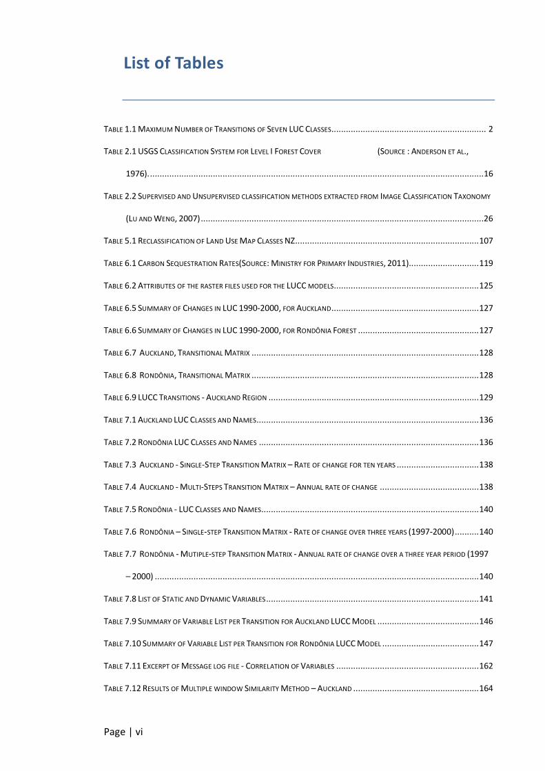
List of Tables ................................................................................................................ vi

List of Abbreviations ................................................................................................... viii

Attestation of Authorship ............................................................................................ ix

Acknowledgements ...................................................................................................... x

Abstract ....................................................................................................................... xi

Chapter 1 Introduction............................................................................................. 1

1.1 Goals .............................................................................................................. 3

1.2 Research Questions ........................................................................................ 4

1.3 Rationale ........................................................................................................ 4

1.4 Significance of the research ............................................................................ 6

1.5 Structure of Thesis .......................................................................................... 7

1.6 Conferences and Publication........................................................................... 9

Chapter 2 Literature Review .................................................................................. 11

2.1 Simulation and Modelling ............................................................................. 11

2.2 Land-Use and Land Cover.............................................................................. 13

2.2.1 Definitions ............................................................................................. 14

2.2.2 Land-use/cover Classification System .................................................... 15

2.3 Land-Use and Cover Change (LUCC) .............................................................. 17

2.3.1 Factors causing LUCC ............................................................................. 17

2.3.2 Effects.................................................................................................... 18

2.3.3 LUCC Variables (Driving Forces) ............................................................. 19

2.3.4 Detecting LUCC ...................................................................................... 20

2.4 Remote Sensing ............................................................................................ 21

Page | ii

2.4.1 Selection of Remotely Sensed Data ........................................................ 22

2.4.2 Determination of a Classification System ............................................... 22

2.4.3 Image Pre-processing............................................................................. 23

2.4.4 Feature Extraction and Selection ........................................................... 23

2.4.5 Selection of Suitable Classification Approach ......................................... 24

2.4.6 Classification Accuracy Assessment ....................................................... 26

2.5 Ancillary Data Integration ............................................................................. 28

2.6 Change Detection ......................................................................................... 28

2.7 Geospatial Analysis ....................................................................................... 30

2.8 LUCC Modelling ............................................................................................ 32

2.8.1 Diversity of LUCC Modelling Methods .................................................... 33

2.8.2 CA and ABM methods ............................................................................ 35

2.9 Cellular Automata LUCC Models ................................................................... 41

2.10 Summary ...................................................................................................... 50

Chapter 3 LUCC Workflow Process Model .............................................................. 51

3.1 Data .............................................................................................................. 51

3.2 Determination of Transition Matrix .............................................................. 53

3.2.1 Definitions and Assumptions ................................................................. 54

3.3 Classification of Continuous Grey scale Variables .......................................... 59

3.3.1 Definitions and Assumptions: Weights of Evidence ................................ 60

3.3.2 Application of WOE in Categorisation of Grey scale Variable ................. 63

3.4 Computation of the WoE Coefficients of Variables ........................................ 65

3.5 Analysis of Variable Correlation .................................................................... 70

3.6 Building and Running LUCC Simulation Model .............................................. 75

3.6.1 LUCC Model Data ................................................................................... 75

3.6.2 Computation of Spatial Transition Probabilities ..................................... 76

3.6.3 Allocation of Simulated Land Changes ................................................... 78

3.6.4 Execution Process of the LUCC Simulation Model .................................. 81

3.7 Validation of the Simulation Model............................................................... 82

Page | iii

3.7.1 Fuzzy Set Theory Approach .................................................................... 86

3.7.2 Validating Model Process or Simulated Map .......................................... 88

Chapter 4 Calibration of LUCC - GA Approach ........................................................ 93

4.1 Definitions .................................................................................................... 94

4.2 GA Working Process for LUCC ....................................................................... 95

Chapter 5 Study Areas.......................................................................................... 100

5.1 Auckland Region - Description .................................................................... 101

5.1.1 The Land and Environment .................................................................. 104

5.1.2 Why Auckland Region? ........................................................................ 108

5.2 Rondônia State – Description ...................................................................... 109

5.2.1 The Land and Environments................................................................. 111

5.2.2 Why the Amazon Forest of Rondônia State? ........................................ 113

5.3 Vegetation Carbon Sequestration ............................................................... 114

5.3.1 Why Carbon Sequestration? ................................................................ 115

5.4 Summary .................................................................................................... 115

Chapter 6 Land Use/Cover Change Model Data.................................................... 116

6.1 Data Description ......................................................................................... 118

6.2 Data Acquisition.......................................................................................... 119

6.3 Data Preparation ........................................................................................ 125

6.3.1 Land Use/Cover Maps .......................................................................... 125

6.4 Drivers of LUCC ........................................................................................... 129

6.5 Summary .................................................................................................... 133

Chapter 7 Implementation and Results ................................................................ 135

7.1 Computation of Transition Matrix of LUCC .................................................. 136

7.1.1 Auckland Region .................................................................................. 136

7.1.2 Rondônia State .................................................................................... 139

7.2 Computation of Weight of Evidence Coefficients ........................................ 140

7.2.1 Weights of Evidence Coefficients – Results and Discussions ................. 147

7.3 Analysing Correlation of Input Variables ..................................................... 159

Page | iv

7.4 Model Execution – Build and Run................................................................ 162

7.5 Validation – Multiple Windows ................................................................... 163

7.6 Enhancement of WoE Coefficients Using GA Tool ....................................... 167

7.6.1 Result of GA Calibration ....................................................................... 170

7.7 Compare GA Calibration with the Primal WoE ............................................ 172

7.8 LUCC Projected Simulation.......................................................................... 174

7.9 Scenario Description ................................................................................... 183

7.9.1 Results and Interpretation ................................................................... 186

7.10 Summary .................................................................................................... 186

Chapter 8 Conclusions and Recommendations..................................................... 188

8.1.1 Investigation of LUCC Modelling Methods ........................................... 188

8.1.2 Review of CA LUCC Models/Software .................................................. 189

8.1.3 LUCC Working Processes ...................................................................... 190

8.1.4 Validating Maps versus Validating Model process ................................ 191

8.1.5 Qualitative vs. Quantitative Validation ................................................. 191

8.1.6 Validation Method ............................................................................... 192

8.1.7 Auckland Data Issues ........................................................................... 193

8.1.8 Calibration and Performance of the LUCC Model ................................. 194

8.2 Limitations of this Work .............................................................................. 195

8.3 Contribution ............................................................................................... 196

8.4 Future Work ............................................................................................... 196

8.5 Conclusion .................................................................................................. 197

REFERENCES ............................................................................................................. 198

Appendix 1 : Dinamica EGO Modelling Software ................................................... 208

Page | i

List of Figures

FIGURE 2.1 THREE DIMENSIONAL FRAMEWORK FOR REVIEWING AND ASSESSING LAND USE CHANGE MODELS (SOURCE:

AGARWAL ET AL., 2002)....................................................................................................................35

FIGURE 2.2 A VISUAL REPRESENTATION OF A CELLULAR AUTOMATA SYSTEM .............................................................36

FIGURE 2.3 A TWO-DIMENSIONAL CA LATTICE (SOURCE: BENENSON & TORRENS, 2004, P.23) ..................................38

FIGURE 2.4 AUTOMATA MOVEMENT IN MULTI-AGENT SYSTEM (SOURCE: BENENSON & TORRENS, 2004, P.23).............40

FIGURE 2.5 LEAM FRAMEWORK (SOURCE: SUN ET AL., 2009). ..........................................................................43

FIGURE 3.1 FLOWCHART OF LUCC WORKFLOW PROCESS ....................................................................................52

FIGURE 3.2 DETERMINATION OF TRANSITION MATRIX, DINAMICA EGO ..............................................................58

FIGURE 3.3 DETERMINATION OF TRANSITION MATRIX FUNCTOR: PORT VIEW ..........................................................59

FIGURE 3.4 GRAPH SHOWING BREAKPOINTS BASED ON THE GREY SCALE VARIABLE ..................................................65

FIGURE 3.5 PORT EDITOR OF DETERMINE WEIGHTS OF EVIDENCE RANGES FUNCTOR .................................................66

FIGURE 3.6 FUNCTOR EDITOR OF DETERMINE WEIGHTS OF EVIDENCE RANGES FUNCTOR ............................................66

FIGURE 3.7 SAMPLE RESULTS OF WOE COEFFICIENTS ........................................................................................68

FIGURE 3.8 GRAPHS OF WOE VS. RANGES ......................................................................................................68

FIGURE 3.9 MESSAGE LOG OF WEIGHTS OF EVIDENCE .......................................................................................69

FIGURE 3.10 SAMPLE - ANALYSIS OF VARIABLE CORRELATION .............................................................................74

FIGURE 3.11 LUCC SIMULATION MODEL IMPLEMENTATION – DINAMICA EGO DESIGN .........................................77

FIGURE 3.12 FLOWCHART OF LUCC MODELLING ..............................................................................................78

FIGURE 3.13 PKL ARRAYS BEFORE [A] AND AFTER [B] CONVOLUTION OF EXPANDER (SOURCE : SOARES-FILHO ET AL., 2002,

P.23). ...........................................................................................................................................80

FIGURE 3.14 GENERATION OF CELLS AROUND ALLOCATED CORE CELL BY PATCHER .....................................................80

FIGURE 3.15 MAP COMPARISON OF CHECKER BOARDS......................................................................................84

FIGURE 3.16 VALIDATION OF LUCC MODEL – OVERALL SIMILARITY ......................................................................89

FIGURE 3.17 VALIDATION OF LUCC MODEL - MULTIPLE WINDOW OF SIMILARITY ....................................................90

FIGURE 3.18 RECIPROCAL SIMILARITY FUNCTOR ...............................................................................................91

Page | ii

FIGURE 3.19 RECIPROCAL SIMILARITY - FUZZY COMPARISON METHOD (SOURCE :SOARES-FILHO ET AL., 2009, P.75) ........91

FIGURE 4.1 WORKFLOW OF GA PROCESS........................................................................................................96

FIGURE 4.2 DESIGN OF GA LUCC CALIBRATION PROCESS ...................................................................................97

FIGURE 5.1 LOCATION OF AUCKLAND REGION IN NEW ZEALAND AND LAND USE MAP ............................................. 102

FIGURE 5.2 POPULATION OF AUCKLAND REGION : 1991 -2006 CEMSUS, 2011 -2031 PROJECTIONS (SOURCE : STATISTICS

NEW ZEALAND, 2009A) .................................................................................................................. 103

FIGURE 5.3 POPULATION DENSITY (PERSONS PER KM2) AUCKLAND REGION. CENSUS 1991-2006, PROJECTION 2011 -2031.

(SOURCE : STATISTICS NEW ZEALAND,2009A) ...................................................................................... 104

FIGURE 5.4 LAND USE MAP OF AUCKLAND REGION ......................................................................................... 108

FIGURE 5.5 RONDÔNIA STATE ITS REGIONAL BLOCKS. THE INSERT MAP, THE RED IS RONDÔNIA LOCATION IN BRAZIL. ........ 110

FIGURE 5.6 STUDY AREA WITH RESPECT TO RONDÔNIA STATE AND BRAZIL ............................................................. 111

FIGURE 5.7 LUC MAP (2000) OF STUDY AREA RONDÔNIA STATE (RED IS NON-VEGETATION LAND, GREEN IS FOREST LAND

AND BLUE IS DEFORESTED LAND) ......................................................................................................... 113

FIGURE 6.1 RASTERISATION OF VECTOR DATA ................................................................................................ 117

FIGURE 6.2 ILLUSTRATION OF LUC DATA AND TIME FRAME ............................................................................... 118

FIGURE 6.3 LUCAS LAND USE MAP OF NEW ZEALAND – 1990, RED BOX INDICATES THE AUCKLAND CASE STUDY REGION. 121

FIGURE 6.4 DIGITAL ELEVATION MODEL (2M), AUCKLAND REGION ..................................................................... 122

FIGURE 6.5 HILLSHADE, AUCKLAND REGION .................................................................................................. 123

FIGURE 6.6 SLOPE, AUCKLAND REGION ........................................................................................................ 124

FIGURE 6.7 DISTANCE-TO-MAJOR ROADS ..................................................................................................... 131

FIGURE 6.8 DISTANCE-TO-MINOR ROADS ..................................................................................................... 131

FIGURE 6.9 DISTANCE-TO-RIVERS ................................................................................................................ 132

FIGURE 6.10 CREATING STACK MAP OF STATIC VARIABLES IN DINAMICA EGO .................................................... 133

FIGURE 7.1 DINAMICA EGO - DETERMINATION OF TRANSITION MATRICES ......................................................... 137

FIGURE 7.2 CATEGORISATION OF GREY SCALE VARIABLE ELEVATION FOR THE TRANSITION 3->2. RED CIRCLE INDICATES THE

PARAMETERS FOR CATEGORISATION. ................................................................................................... 142

FIGURE 7.3 COMPUTATION OF WEIGHTS OF EVIDENCE RANGES AND COEFFICIENTS ................................................ 143

FIGURE 7.4 EXAMPLE OF WOE OF VARIABLES SHOWING INFLUENCE ON TRANSITION ................................................ 144

FIGURE 7.5 EXAMPLE OF WOE OF VARIABLES SHOWING NO INFLUENCE ON TRANSITION ........................................... 145

FIGURE 7.6 DIST. TO MINOR ROADS [1->2) .................................................................................................. 149

Page | iii

FIGURE 7.7 DIST. TO OTHERS ..................................................................................................................... 149

FIGURE 7.8 DIST. TO SETTLEMENTS ............................................................................................................. 149

FIGURE 7.9 DIST. TO PLANTED FOREST ......................................................................................................... 149

FIGURE 7.10 ELEVATION [1->3] ................................................................................................................. 150

FIGURE 7.11 DIST. TO GRASSLAND [1->3] .................................................................................................... 150

FIGURE 7.12 DIST. TO MAJOR ROADS [1->3] ................................................................................................ 150

FIGURE 7.13 DIST. TO PLANTED FOREST [1->3] ............................................................................................. 150

FIGURE 7.14 RESERVED LANDS [1->3] ......................................................................................................... 150

FIGURE 7.15 DIST. TO RIVERS [1->3] .......................................................................................................... 150

FIGURE 7.16 DIST. TO SETTLEMENTS [1->3].................................................................................................. 150

FIGURE 7.17 SLOPE [1->3] ....................................................................................................................... 150


FIGURE 7.19 DIST. TO MAJOR ROADS .......................................................................................................... 151

FIGURE 7.20 DIST. TO NATURAL FOREST....................................................................................................... 151

FIGURE 7.21 DIST. TO OTHER LANDS ........................................................................................................... 152

FIGURE 7.22 DIST. TO SETTLEMENTS ........................................................................................................... 152



FIGURE 7.25 DIST. TO MINOR ROADS [3->2] ................................................................................................ 152

FIGURE 7.26 DIST. NATURAL FOREST [3->2] ................................................................................................. 152





FIGURE 7.31 SLOPE [3->2] ....................................................................................................................... 153




FIGURE 7.35 DIST. TO NATURAL FOREST [3->6] ............................................................................................. 154

FIGURE 7.36 DIST. TO OTHER [3->6] .......................................................................................................... 154

Page | iv





FIGURE 7.41 SLOPE [3->6] ....................................................................................................................... 155








FIGURE 7.49 DISTANCE TO DEFORESTED LANDS .............................................................................................. 157

FIGURE 7.50 ELEVATION ........................................................................................................................... 157

FIGURE 7.51 DISTANCE TO ALL ROADS .......................................................................................................... 158

FIGURE 7.52 DISTANCE TO MAJOR RIVERS ..................................................................................................... 158

FIGURE 7.53 DISTANCE TO SETTLEMENTS ...................................................................................................... 158

FIGURE 7.54 DISTANCE TO TRANS-RIVERS ..................................................................................................... 158

FIGURE 7.55 PROTECTED AREAS ................................................................................................................. 158

FIGURE 7.56 SLOPE ................................................................................................................................. 158

FIGURE 7.57 SOIL ................................................................................................................................... 158

FIGURE 7.58 URBAN ATTRACTION ............................................................................................................... 158

FIGURE 7.59 VEGETATION ......................................................................................................................... 159

FIGURE 7.60 DETERMINING CORRELATION OF VARIABLES ................................................................................. 160

FIGURE 7.61 LUCC MODEL EXECUTION IN DINAMICA EGO........................................................................... 161

FIGURE 7.62 MULTIPLE WINDOWS VALIDATION ............................................................................................. 165

FIGURE 7.63 LUCC MODEL FITNESS – AUCKLAND REGION ............................................................................... 166

FIGURE 7.64 LUCC MODEL FITNESS – RONDÔNIA REGION .............................................................................. 167

FIGURE 7.65 GA CALIBRATION MODEL - DINAMICA EGO .............................................................................. 169

FIGURE 7.66 THE GA TOOL ...................................................................................................................... 170

Page | v

FIGURE 7.67 GRAPH OF BEST-FITNESS OF THE BOUNDARIES .............................................................................. 171

FIGURE 7.68 COMPARISON OF BOUNDARY LIMITS OF GA TOOL .......................................................................... 172

FIGURE 7.69 PERFORMANCE COMPARISON OF ORIGINAL WOE AND GA GENERATED WOE ....................................... 173

FIGURE 7.70 TREND OF LUCC SIMULATION 1990-2050 ................................................................................. 176

FIGURE 7.71 THE TREND OF LUCC FOR THE CENTRAL FOREST REGION OF RONDÔNIA .............................................. 177

FIGURE 7.72 SAMPLE OF SIMULATED LUCC MAPS OF RONDÔNIA ...................................................................... 178

FIGURE 7.73 NATURAL FOREST TO PLANTED FOREST ....................................................................................... 179

FIGURE 7.74 NATURAL FOREST TO GRASSLAND .............................................................................................. 179

FIGURE 7.75 NATURAL FOREST TO SETTLEMENTS ............................................................................................ 179

FIGURE 7.76 PLANTED FOREST TO GRASSLAND ............................................................................................... 179

FIGURE 7.77 GRASSLAND TO PLANTED FOREST ............................................................................................... 180

FIGURE 7.78 GRASSLAND TO SETTLEMENTS ................................................................................................... 180

FIGURE 7.79 GRASSLAND TO OTHER LANDS ................................................................................................... 180

FIGURE 7.80 OTHERS TO PLANTED FOREST .................................................................................................... 180

FIGURE 7.81 OTHERS TO GRASSLAND .......................................................................................................... 181

FIGURE 7.82 OTHERS TO SETTLEMENTS ........................................................................................................ 181

FIGURE 7.83 SIMULATED LUC MAPS 1991 AND 2050 .................................................................................... 182

FIGURE 7.84 ANNUAL CARBON SEQUESTRATION BY VEGETATION ....................................................................... 184

FIGURE 7.85 CARBON SEQUESTRATION SCENARIO MODEL ................................................................................ 185

FIGURE A1.1 DINAMICA EGO OVERVIEW (SOURCE: SOARES-FILHO, 2012) ....................................................... 209

FIGURE A1.2 DINAMICA EGO SOFTWARE ARCHITECTURE .............................................................................. 210

FIGURE A1.3 BASIC DATAFLOW STRUCTURE .................................................................................................. 212

FIGURE A1.4 FUNCTOR PORT EDITOR OF DETERMINE TRANSITION MATRIX ........................................................... 213

Page | vi

List of Tables

TABLE 1.1 MAXIMUM NUMBER OF TRANSITIONS OF SEVEN LUC CLASSES ................................................................ 2

TABLE 2.1 USGS CLASSIFICATION SYSTEM FOR LEVEL I FOREST COVER (SOURCE : ANDERSON ET AL.,

1976). ..........................................................................................................................................16

TABLE 2.2 SUPERVISED AND UNSUPERVISED CLASSIFICATION METHODS EXTRACTED FROM IMAGE CLASSIFICATION TAXONOMY

(LU AND WENG, 2007) .....................................................................................................................26

TABLE 5.1 RECLASSIFICATION OF LAND USE MAP CLASSES NZ............................................................................ 107

TABLE 6.1 CARBON SEQUESTRATION RATES(SOURCE: MINISTRY FOR PRIMARY INDUSTRIES, 2011)............................. 119

TABLE 6.2 ATTRIBUTES OF THE RASTER FILES USED FOR THE LUCC MODELS ............................................................ 125

TABLE 6.5 SUMMARY OF CHANGES IN LUC 1990-2000, FOR AUCKLAND ............................................................. 127

TABLE 6.6 SUMMARY OF CHANGES IN LUC 1990-2000, FOR RONDÔNIA FOREST .................................................. 127

TABLE 6.7 AUCKLAND, TRANSITIONAL MATRIX .............................................................................................. 128

TABLE 6.8 RONDÔNIA, TRANSITIONAL MATRIX .............................................................................................. 128

TABLE 6.9 LUCC TRANSITIONS - AUCKLAND REGION ....................................................................................... 129

TABLE 7.1 AUCKLAND LUC CLASSES AND NAMES............................................................................................ 136

TABLE 7.2 RONDÔNIA LUC CLASSES AND NAMES ........................................................................................... 136

TABLE 7.3 AUCKLAND - SINGLE-STEP TRANSITION MATRIX – RATE OF CHANGE FOR TEN YEARS .................................. 138

TABLE 7.4 AUCKLAND - MULTI-STEPS TRANSITION MATRIX – ANNUAL RATE OF CHANGE ......................................... 138

TABLE 7.5 RONDÔNIA - LUC CLASSES AND NAMES.......................................................................................... 140

TABLE 7.6 RONDÔNIA – SINGLE-STEP TRANSITION MATRIX - RATE OF CHANGE OVER THREE YEARS (1997-2000) .......... 140

TABLE 7.7 RONDÔNIA - MUTIPLE-STEP TRANSITION MATRIX - ANNUAL RATE OF CHANGE OVER A THREE YEAR PERIOD (1997

– 2000) ...................................................................................................................................... 140

TABLE 7.8 LIST OF STATIC AND DYNAMIC VARIABLES ........................................................................................ 141

TABLE 7.9 SUMMARY OF VARIABLE LIST PER TRANSITION FOR AUCKLAND LUCC MODEL .......................................... 146

TABLE 7.10 SUMMARY OF VARIABLE LIST PER TRANSITION FOR RONDÔNIA LUCC MODEL ........................................ 147

TABLE 7.11 EXCERPT OF MESSAGE LOG FILE - CORRELATION OF VARIABLES ........................................................... 162

TABLE 7.12 RESULTS OF MULTIPLE WINDOW SIMILARITY METHOD – AUCKLAND .................................................... 164

Page | vii

TABLE 7.13 RESULTS OF MULTIPLE WINDOW SIMILARITY METHOD - RONDÔNIA ..................................................... 164

TABLE 7.14 BEST-FITNESS OF THE BOUNDARIES. ............................................................................................. 170

TABLE 7.15 GA PERFORMANCE WITH RESPECT TO BOUNDARY LIMITS OF PRIMAL SET OF WOE. .................................. 171

TABLE 7.16 PERFORMANCE COMPARISON OF PRIMAL-WOE AND GA-WOE ......................................................... 173

TABLE 7.17 CELL COUNT OF SIMULATED LUC MAPS - AUCKLAND ........................................................................ 175

TABLE 7.18 PERCENTAGE OF SIMULATED CHANGE BASED ON THE 1990 LUC OF AUCKLAND...................................... 175

TABLE 7.19 CELL COUNT OF SIMULATED LUC MAPS – RONDÔNIA ....................................................................... 175

TABLE 7.20 PERCENTAGE OF SIMULATED CHANGE BASED ON 1997 LUC MAP OF RONDÔNIA .................................... 175

TABLE 7.21 CARBON SEQUESTRATION RATES(SOURCE: MINISTRY FOR PRIMARY INDUSTRIES, 2011)........................... 184

Page | viii

List of Abbreviations

Abbreviations Meaning

ABM Agent Based Model

CA Cellular Automata

LUC Land Use/Cover

LUCC Land Use Cover Change

GIS Geographic Information System

RS Remote Sensing

SLEUTH Slope, Land use, Elevation, Urban, Transportation, Hillshade

UGM Urban Growth

LCD Land Cover Deltatron

MC Monte Carlo

MOLAND Modelling of Land Use/Cover Dynamics

LEAM Land-use Evolution and Impact Assessment

GCP Ground Control Point

ANN Artificial Neural Network

MAS Multi-Agent Simulation

KQML Knowledge Query Manipulation Language

GUI Graphical User Interface

WoE Weights of Evidence

NZ New Zealand

Dist. Distance

RMSE Root Mean Square Error

Page | ix

Attestation of Authorship

I hereby declare that this submission is my own work and that, to the best of my

knowledge and belief, it contains no material previously published or written by

another person (except where explicitly defined in the acknowledgements), nor

material which to a substantial extent has been submitted for the award of any other

degree or diploma of a university or other institution of higher learning.

-----------------------------------------------------

Isaac Kwadwo Nti

Date: 28 November 2013

Page | x

Acknowledgements

This doctoral thesis would not have been possible without the help and the guidance of several individuals who in diverse ways contributed and extended their valuable assistance in the preparation and completion of this study.

First and foremost, my deepest appreciation to my primary supervisor, Prof Philip Sallis, for his excellent support, inspiration, guidance, caring, and provision of an excellent atmosphere for conducting this research. His rich experience always took the struggle of this journey.

My sincere gratitude goes to my secondary supervisor, Dr. Subana Shanmuganathan, who helped me with data acquisition and also for being generous with her time and comments.

My colleagues and the staff at Geo-informatics Research Centre (GRC) also deserve my sincerest thanks, their friendship and assistance has meant more to me than I could express. I also thank GRC for sponsoring my trip to Centro de Sensoriamento Remoto (CSR) lab in Brazil for part of my lab work.

Special thanks to the Faculty of Design and Creative Technologies, AUT for the award of Graduate Assistant which included my fees and a monthly stipend. This really relieved me of financial worries.

The members of CSR lab especially Prof Britaldo Soares-Filho, Hermann Rodrigues and Leticia Lima have been of immense support to me. I made remarkable achievement when I used their lab for a month.

The GIS Department of Auckland Region Council, for giving their high resolution aerial photographs and Digital Elevation Model data for my work.

My friend, Dr Mark von Veh, for his insights and rich experience in land use cover data of New Zealand especially in the area of forestry management.

Michael Franklin Bosu, a childhood friend currently doing his PhD at AUT for proofreading each chapter of my work.

My utmost gratitude to my wife Mansa Nti and children - Jeremy, Jaydon and Jonelle - for their encouragement and unflinching support at all times.

And above all, to the Omniscient and Omnipresent God, for giving me the strength to plod on despite my constitution wanting to give up and throw in the towel, thank you so much Heavenly Father.

Page | xi

Abstract

Human activities and effects of global warming are increasingly changing the physical

landscape. In view of this researchers have developed models to investigate the cause

and effect of such variations. Most of these models were developed for specific

locations with spatial variables causing change for that location. Also the application

areas of these models are mainly binary transitions, not complex models which involve

multiple transitions, for example deforestation models which deal with the transition

from forest lands to non-forest areas and urban growth transition from non-urban

areas to urban. Moreover these land simulation models are closed models because

spatial variables cannot be introduced or removed, rather modellers can only modify

the coefficients of the fixed variables. Closed models have significant limitations largely

because geospatial variables that cause change in a locality may differ from one

another. Thus with closed models the modellers are unable to measure and test the

significance of variables before their inclusion.

This work investigated existing land use cover change (LUCC) models and aimed to find

a geospatial workflow process modelling approach for LUCC so that the influence of

geospatial variables in LUCC could be measured and tested before inclusion. The

derived geospatial workflow process was implemented in DINAMICA EGO, an open

generic LUCC modelling environment. For the initial calibration phase of the process

the Weight of Evidence (WoE) method was used to measure the influence of spatial

variables in LUCC and also to determine the variables significance. A Genetic Algorithm

was used to enhance the WoE coefficients and give the best fitness of the coefficients

Page | xii

for the model. The model process was then validated using kappa and fuzzy similarity

map comparison methods, in order to quantify the similarity between the observed

and simulated spatial pattern of LUCC.

The performance of the workflow process was successfully evaluated using the

Auckland Region of New Zealand and Rondônia State of Brazil as the study areas. The

Auckland LUCC model was extended to demonstrate vegetative carbon sequestration

scenario. Ten transitions were modelled involving seven Land Use Cover (LUC) classes

and a complex dynamic LUCC for Auckland was generated. LUC maps for 1990 and

2000 were used to calibrate the model and 2008 was used to validate the model. The

static spatial variables tested were road networks, river networks, slope, elevation,

hillshade, reserved lands and soil. The hillshade and soil variables were found to have

no significant impact in the LUCC for the Auckland area, therefore they were excluded

from the model. If a closed model had been used these insignificant variables would

have been included. The calibration phase revealed that wetland and cropland LUC

areas in Auckland have not changed between 1990 and 2000. The validated LUCC

model of Auckland, served as a foundation for simulating annual LUC maps for advance

modelling of Carbon Sequestration by vegetation cover.

In order to test the generic nature of the workflow process model a second case study

was introduced that had a different data resolution, area extent and fewer LUC

transitions. Compared to Auckland, the new Rondônia case study was a simple LUCC

model with only one transition, with coarse data resolution (250m) and large area

extent. The evaluation of the Rondônia LUCC model also gave good result. It was then

concluded that the derived workflow process model is generic and could be applied to

any location.

Page | 1

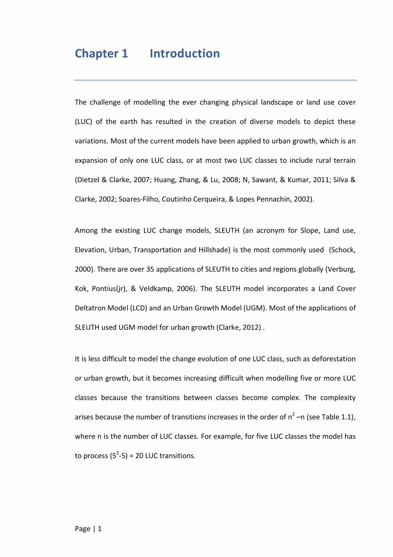
Chapter 1 Introduction

The challenge of modelling the ever changing physical landscape or land use cover

(LUC) of the earth has resulted in the creation of diverse models to depict these

variations. Most of the current models have been applied to urban growth, which is an

expansion of only one LUC class, or at most two LUC classes to include rural terrain

(Dietzel & Clarke, 2007; Huang, Zhang, & Lu, 2008; N, Sawant, & Kumar, 2011; Silva &

Clarke, 2002; Soares-Filho, Coutinho Cerqueira, & Lopes Pennachin, 2002).

Among the existing LUC change models, SLEUTH (an acronym for Slope, Land use,

Elevation, Urban, Transportation and Hillshade) is the most commonly used (Schock,

2000). There are over 35 applications of SLEUTH to cities and regions globally (Verburg,

Kok, Pontius(jr), & Veldkamp, 2006). The SLEUTH model incorporates a Land Cover

Deltatron Model (LCD) and an Urban Growth Model (UGM). Most of the applications of

SLEUTH used UGM model for urban growth (Clarke, 2012) .

It is less difficult to model the change evolution of one LUC class, such as deforestation

or urban growth, but it becomes increasing difficult when modelling five or more LUC

classes because the transitions between classes become complex. The complexity

arises because the number of transitions increases in the order of n2 –n (see Table 1.1),

where n is the number of LUC classes. For example, for five LUC classes the model has

to process (52-5) = 20 LUC transitions.

Page | 2

Class 1 Class 2 Class 3 Class 4 Class 5 Class 6 Class 7

Class 1 ---------- 1-to-2(1) 1-to-3(3) 1-to-4(7) 1-to-5(13) 1-to-6(21) 1-to-7(31)

Class 2 2-to-1(2) ---------- 2-to-3(4) 2-to-4(8) 2-to-5(14) 2-to-6(22) 2-to-7(32)

Class 3 3-to-1(5) 3-to-2(6) ---------- 3-to-4(9) 3-to-5(15) 3-to-6(23) 3-to-7(33)

Class 4 4-to-1(10) 4-to-2(11) 4-to-3(12) ---------- 4-to-5(16) 4-to-6(24) 4-to-7(34)

Class 5 5-to-1(17) 5-to-2(18) 5-to-3(19) 5-to-4(20) ---------- 5-to-6(25) 5-to-7(35)

Class 6 6-to-1(26) 6-to-2(27) 6-to-3(28) 6-to-4(29) 6-to-5(30) ---------- 6-to-7(36)

Class 7 7-to-1(37) 7-to-2(38) 7-to-3(39) 7-to-4(40) 7-to-5(41) 7-to-6(42) ----------

Table 1.1 Maximum Number of Transitions of Seven LUC Classes

An additional issue is that the inherent error of each transition contributes to the

overall error of the calibration and validation of the model, making it difficult to arrive

at a precise “best fit” result. For instance a LUC change model of seven classes will

have a maximum of 42 transitions as shown in Table 1.1, therefore the best-fit value of

such model will incorporate the sum of all inherent errors from the 42 transitions.

Another challenge is the determination of reaching a satisfactory degree of

significance for drivers/parameters/variable values for inclusion in a land use cover

change (LUCC) model. Most of the LUC change models were developed for either

specific projects or locations therefore they are not generic and cannot be adapted for

other locations. Although the SLEUTH model and others (Mas et al., 2007; Verburg,

Schot, Dijst, & Veldkamp, 2004) have been applied to many locations globally,

modellers are unable to modify the drivers influencing the change because the

assumption is that the drivers of change are the same at every location, this is a

fundamental conceptual flaw. When applying such models to different locations,

modellers can only adjust the coefficients of the parameters during the calibration

phase. In such models the variables are predefined. For this reason a generic modelling

environment and workflow process for LUCC, which will allow modellers to determine

To From

Page | 3

the significance of a driving force, would be a great improvement on the current

models available.

Landscape modelling is a dynamic field of study where many models are developed,

tested, refined, adopted for further use or discarded. Despite some of the advances in

the LUC modelling domain, there still seems to be a lack of generic

platforms/software/tools that incorporate all the useful features and processes that

have been developed to date. A modelling environment that combined these features

would give modellers the control to design and implement their own LUCC models and

scenarios.

1.1 Goals

The research described in this thesis aims to investigate existing LUCC methods,

models and tools with a view to deriving a generic integrated workflow process for

LUCC modelling. As a result of this investigation a generic LUCC model will be

developed that can be used as a framework to investigate and model a broad range of

possible LUCC scenarios. The framework’s effectiveness and the degree to which the

framework is generic will be evaluated using three different case studies; the Auckland

Region of New Zealand, the Rondônia State in Brazil and a Carbon Sequestration

Scenario model for the Auckland Region. The evaluation will involve:

Conceptualizing and designing LUCC models for two study areas – Auckland

Region and Rondônia State – based on the workflow process.

Calibrating the LUCC models

Validating the LUCC models

A comparative analysis of the results of the two case studies specifically

examining the effect of resolution, scale, rate of LUCC and class complexity.

Page | 4

Using a validated LUCC model, as a base model for advanced modelling and

prediction using a carbon sequestration scenario model for the Auckland

region.

1.2 Research Questions

The primary research questions for this research are:

1. How can we measure the 'adequacy' of the components, variables and

parameter sets, which combine to inform the development of an LUCC model?

1.1 What approaches are appropriate for this measurement of adequacy?

2. What are the core processes within a generic geospatial LUCC framework?

2.1 How do we measure the performance of these processes?

The framework that will be developed and evaluated in this research will be designed

based on the following assumptions:

There is an integrated workflow process.

For LUCC modelling, there must be an interrelated set of variables influencing

the change. These variables are inherently complex and the complexity arises

from the number of transitional changes.

Selection of variables is not in any way constrained. Any variables can be

included in the initial variable set. These variables are automatically evaluated

and the ones that do not influence LUCC will be eliminated prior to modelling.

1.3 Rationale

LUCC simulation models play an important role in the analysis of causes and impact of

change in the environment and landscape. Geographic Information Systems (GIS) and

Remote Sensing (RS) are becoming increasingly popular in landscape management

Page | 5

primarily because of their functionalities and capabilities. These techniques consist of

functions that capture, store, analyse, manipulate and display spatial data. With GIS

and RS it is relatively straight forward for users to identify what change has occurred

and where it has occurred (Şatır & Berberoğlu, 2012). However, these approaches are

limited because they do not have the capability to explicitly model LUCC transitions

and therefore it is difficult for the users to formulate theories as to the reason for the

change. In contrast, with the aide of LUCC models, modellers are more able to form

theories as to “why” transitional changes have occurred. Therefore LUCC models can

provide better support for decision makers such as planners, engineers and policy

makers. The analysis of the driving factors in LUCC models is what assists modellers

and users in understanding “why” a change has occurred. Since the cause of change is

different for each location and or region there is the need for generic modelling

environment which could be used by LUCC modeller to determine the cause of change

at any location.

The foremost of the many reasons for a generic modelling environment and workflow

process is to determine the adequacy or significance of driving factors for change using

a generic modelling environment. A generic modelling environment will not have

predefined variables for every location; it rather allows the assessment of the

influence of any set of variables for each specific location before inclusion. Such a

system should be able to model a wide range of systems from very simple systems

(with a few parameters) to more complex systems with varying spatial resolutions.

Page | 6

1.4 Significance of the research

The availability of generic workflow process and/or modelling environment for creating

LUCC models has many applications. For instance, it could enable historians to

conduct empirical research on the history of the land use in relation to human

settlement and economic change, and to visualize past landscapes and the change in

the morphology of the built environment over time. Decision makers could analyse

various critical incidences in a society and environment over time in a coherent and

cohesive manner to investigate for example:

1. Land use change

2. changing employment patterns

3. class consciousness and neighbourhood analysis and,

4. the impact of planning processes in rural development

A common framework could be of significant use to landscape planners, such as

engineers, architects, and to a greater extent to policy makers, who are in urgent need

of simulation models for visualizing the potential evolution scenarios of a landscape

based on their current decisions made on the land use / development of a physical

area.

Typical contemporary examples can be drawn from what are famously referred to as

“Cross-cutting issues” (Agarwal, Green, Grove, Evans, & Schweik, 2002). These models

could be used to determine future scenarios, changes to the landscape of an area of

interest under a given number of proposed developmental activities especially, in

performing trade-off analysis studies on the options available to decision-making

professionals, their potential benefits and disadvantages.

Page | 7

The potential, for decision making, of the generic framework developed in this work is

demonstrated by applying the framework to a carbon sequestration study of the

Auckland region.

1.5 Structure of Thesis

The thesis is made up of the following nine chapters as described in this subsection.

Chapter 1: Gives an introduction of the thesis with a brief description of the existing

work and some challenges faced. Also the goals, objectives and research of the thesis

are outlined here. The significance and rationale of this research were included this

chapter.

Chapter 2: Provides a review the theoretical foundation and fundamental concepts for

the “workflow processes” of Land-use/cover change (LUCC). The workflow processes

of relevant LUCC models and their modelling methods were explored. The goal of

investigation into the LUCC workflow process was to generate or derive an open LUCC

workflow process model which could easily be used by users to measure the adequacy

of variables or parameter set of a LUCC model.

Chapter 3: Further explains with detailed equations the methodology used in designing

and implementing LUCC model for the candidate area (Auckland Region). A description

of integrated workflow process model to measure the adequacy and significance of

LUCC model variables is outlined. Details of the Weight of Evidence (WoE) method,

which is used in measuring the adequacy and significance of the LUCC model variables,

are provided. Also the validation of workflow process model is discussed.

Page | 8

Chapter 4: This part of work describes the Genetic Algorithm method of LUCC

calibration which is to enhance the results of the WoE method of calibrating the LUCC

model variables.

Chapter 5: Elaborates on the description of the study areas namely the Auckland

Region and the amazon forest area of Rondônia state, on which the derived workflow

process model will be applied for evaluation.

Chapter 6: This chapter introduces the LUCC data used for LUCC model of Auckland

Region and Rondônia state. A description of the LUC and variable maps is provided and

their acquisition is detailed. . Additionally a description of the methods used for data

format preparation is provided.

Chapter 7: Describes the implementation and results of the workflow process model in

Auckland Region. The method for evaluation and selection of the LUCC models

variables is detailed and critically evaluated. This chapter discusses in detail the

implementation of all the phases/steps in the workflow process model for the

Auckland region and the Rondônia state case studies.

It presents a demonstration of an advanced LUCC modelling of vegetation carbon

sequestration model which is a built up on the LUCC model of Auckland. It reveals the

effect of vegetation change on carbon removal from atmosphere.

Chapter 8: Presents a summary of the results of this research. The contribution this

work has made to existing knowledge is outlined and some limitations of the work

were given. Some suggestions are made regarding further and future work.

Page | 9

1.6 Conferences and Publication

Below are the conference proceedings, abstracts and posters published during the

research for this thesis:

1. Nti, I. K., & Sallis, P. (2013). Geospatial Modelling of Complex Land Use Cover

Change: How to Determine the Adequacy and Significance of Variables. In A. Moore

& P. A. Whigham (Eds.), Proceedings of the SIRC NZ Conference. Presented at the

SIRC NZ - GIS and Remote Sensing Research Conference.

2. Nti, I. and Sallis, P. (2012). Modelling Dynamic Land-Use/Cover Change in Auckland

Region. Fourth Digital Earth Summit, Wellington, New Zealand, 2-4 September

2012.

3. Owusu-Banahene W., Nti I., & Sallis P. (2011). Integrating geo-spatial information

infrastructure into conservation and management of wetlands in Ghana. Second

International Conference on Intelligent Systems, Modelling and Simulation, 2011.

24 & 27-28 JANUARY 2011, Kuala Lumpur, Malaysia & Phnom Penh, Cambodia

ISMS2011. ISBN 978-0-7695-4336-9/11 © 2011 IEEE DOI 10.1109/ISMS.2011.24.

pp. 91-94.

4. Hock, B., Nti, I. and Sallis, P. (2010). Geovisualisation of land use in rivers:

visualisations of the downstream effects of the rural lands of New Zealand.

GeoCart’2010 and ICA Symposium on Cartography, Auckland, New Zealand, 1-3

September 2010.

5. Owusu-Banahene, W.; Nti, I.K.; Sallis, P.J.; , Developing a Geo-spatial Information

Framework to Facilitate National Identification System (NIS) in Ghana, Computer

Modeling and Simulation (EMS), 2010 Fourth UKSim European Symposium on , vol.,

no., pp.68-74, 17-19 Nov. 2010. doi: 10.1109/EMS.2010.112

6. Nti, I., Sallis, P. and Shanmuganathan, S. (2009). Landscape visualisation for frost

events in vineyards. New Zealand Postgraduate Conference 20-21 Nov 09,

Wellington, New Zealand. (The above poster had been awarded the "University of

Canterbury award for outstanding visual presentation" in the NZ Post Graduate

Conference, 2009)

Page | 10

7. Nti, K., Sallis, P. and Shanmuganathan, S. (2009). A review on techniques applied to

modelling, simulating and visualising evolution of physical landscape. 2009

International Conference on Computational Intelligence, Modelling and Simulation.

pp. 54-58.

Page | 11

Chapter 2 Literature Review

In this chapter, the theories and foundations of the “workflow processes” of LUCC

models are reviewed and summarised. In the many studies reviewed, the processes

developed for modelling, simulating and visualizing a landscape have made use of a

number of different frameworks and factors. These are investigated as a basis for

constructing a unified framework designed especially for continuously monitoring the

various changes that a physical landscape could undergo over a period of time. Many

of these existing models are implemented using a Geographic Information System

(GIS) but some utilise multi-agent based simulation software or integrate GIS with

Cellular Automata algorithms.

This chapter begins by examining the terminology used in LUCC modelling and the

methodology used to assess the evolution of LUC (land use cover). Various working

models developed over the past few years are then outlined and critiqued.

2.1 Simulation and Modelling

Bellinger (2004, p.1) refers to a model as being a “simplified representation of a

system at some particular point in time or space intended to promote understanding

of the real system” whilst “simulation is the manipulation of a model in such a way

that it operates on time or space to represent it, thus enabling one to perceive the

interactions that would not otherwise be apparent because of their separation in time

or space”. Guizani et al. (2010, p.1) also defines Simulation as the “imitation of a real-

world system through a computational re-enactment of its behaviour according to the

Page | 12

rules described in a mathematical model”. Simulation can or may replicate a real

system or process. The process of simulation usually entails looking at a limited

number of key features and functions within the physical or abstract system of

interest, which is normally complex and detailed. A simulation enables users to analyse

the system’s behaviour under varying scenarios, through the re-enactment within a

virtual computational environment (Guizani et al., 2010).

Simulation is applied in many contexts including natural systems such as LUCC to gain

insight into its functioning. Regarding simulation the important issues include:

acquisition of valid source information about system of reference, example

landscape

extraction of important features

simplifying approximations and assumptions

calibration and validation

Simulation is an important approach in scientific research because it facilitates

research involving systems and or processes with time dependent behaviour.

Models can be classified as continuous or discrete state models based on the values

of the state variables. A model is a continuous state model if the variable can assume

any value at any instant in time and a discrete state model when it assumes a single

value at a point in time. A discrete state model could further be classified as

continuous or discrete time model. A continuous time model is when the state

variable can change at any time and it is discrete time if the state variable can change

their values at a discrete time instant. This research develops a discrete time model

Page | 13

where the state variable is the yearly LUCC. Most discrete time event driven

simulations rely on underlying equations to manage the event in time but automata

models (including agent-based cellular automata models) do not. In automata models,

the automata – cell or agent (trees, humans, land use cover) – in the model are directly

represented and possess an internal state and set of rules which determine how the

agent state is update from one step to the next (Bellinger, 2004; Guizani et al., 2010).

Deterministic and probabilistic models: If repeating the same input – starting

conditions or initial state - always produces the same output then the model is

deterministic whilst it is probabilistic or stochastic if the output keeps changing due to

the randomness of variables. A deterministic model has no random variable(s) whilst

probabilistic have at least one random variable as input (Gibb, St-Jacques, Nourry, &

Johnson, 2002).

A model is said to be open if it is able in take one or more external inputs, on the other

hand it is called closed model if it has no external inputs (Guizani et al., 2010 p.5) .

LUCC simulation models are mainly event-driven therefore dynamic (change over time)

in nature. This research seeks to review LUCC simulation models in order to find an

open and or generic modelling framework or environment which allows the external

variables as input.

2.2 Land-Use and Land Cover

Even though land-use and land cover are definitely related the two are conceptually

different (Gregorio & Jansen, 2005; Fisher & Unwin, 2005). Many researchers do not

acknowledge this distinction and tend to use these terms interchangeably (Gregorio &

Page | 14

Jansen, 2005; Fisher & Unwin, 2005). I seek to reveal the difference and the

relationship between land use and land cover.

2.2.1 Definitions

In terms of remote sensing and photogrammetry, Fisher and Unwin (2005) define land-

cover as “the physical material at the surface of the earth. It is the material that we see

and which directly interacts with electromagnetic radiation and causes the level of

reflected energy that we observe as the tone or the digital number at a location in an

aerial photograph or satellite image”. According to Ellis and Pontius (2010) land cover

refers to the physical and biological cover over the surface of land, including water,

vegetation, bare soil, and/or artificial structures.

In agriculture land-use is typically described in terms of the total activities (for example

irrigation, crop rotation and other crop management practices) that individuals

undertake within a specific land cover type (Swanson, Bentz, and Sofranko (1997).

Land planners and social scientists generally refer to land-use as comprising of the

social and economic practices on the land. Natural scientists categorise land-use in

relation to the results of human activities such as forestry, agricultural and building

(Ellis & Pontius, 2010). Therefore land-use is the classification of how the land is used.

Despite the fact that land-cover and land-use are distinct in definition they have an

intricate relationship. For example a land-cover type grass can occur in many land-

uses, built-up areas, parks, and croplands. However, only a few regions of homogenous

land-use have a single land-cover; settlements for instance may have grass, shrubs,

trees and buildings as land-cover. Also a parcel of land-cover can have multiple land-

Page | 15

uses; a planted forest might be used for hiking, trekking and hunting and perhaps

grazing.

Land-cover is important for the design and implementation of physical and

environmental models. Additionally, it is indirectly helpful for many policy and

planning models where land-use is the appropriate concept. In view of this, the term

land-use/cover (LUC) will be the term adopted in this thesis referring to the physical

land-cover of the land-use practice.

2.2.2 Land-use/cover Classification System

LUC is usually categorised into various classes for the purposes of mapping, town and

country planning, nature conversation etc. Sokal (1974, p.1116) defines classification

as “the ordering or arrangement of objects into groups or sets on the basis or their

relationships”. LUC classification describes a systematic framework with the names of

classes and the standards used to differentiate them, and the relationships amongst

the classes. It is often an extensive standardised a priori classification method

developed to meet certain user specifications and made for mapping procedures,

regardless of the scale or method used to map (Anderson, Hardy, Roach, & Witmer,

1976; Gregorio & Jansen, 2005; Şatır & Berberoğlu, 2012). There are several LUC

classification systems used by remote sensing and LUC cartographers today; some are

designed for national purposes while others have been adopted for global use due to

the versatile nature of the classifiers. Two of the major LUC classification systems

mostly used are:

Page | 16

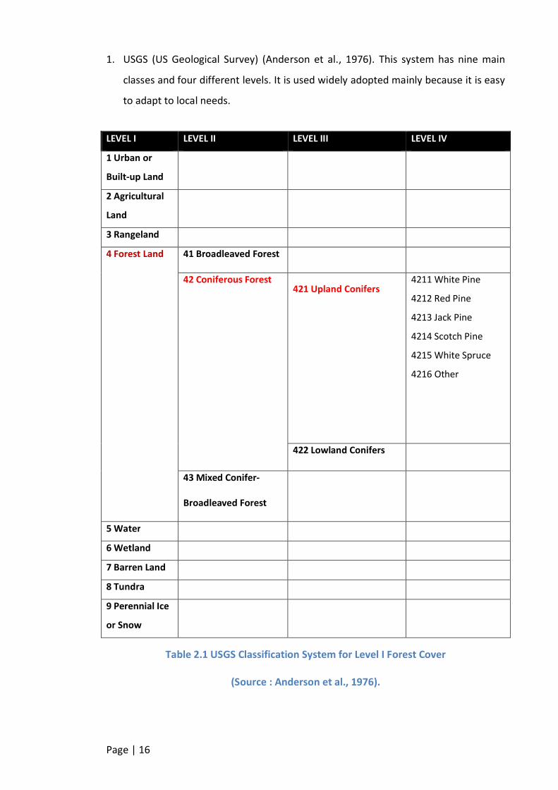
1. USGS (US Geological Survey) (Anderson et al., 1976). This system has nine main

classes and four different levels. It is used widely adopted mainly because it is easy

to adapt to local needs.

LEVEL I LEVEL II LEVEL III LEVEL IV

1 Urban or

Built-up Land

2 Agricultural

Land

3 Rangeland

4 Forest Land 41 Broadleaved Forest

42 Coniferous Forest 421 Upland Conifers

4211 White Pine

4212 Red Pine

4213 Jack Pine

4214 Scotch Pine

4215 White Spruce

4216 Other

422 Lowland Conifers

43 Mixed Conifer-

Broadleaved Forest

5 Water

6 Wetland

7 Barren Land

8 Tundra

9 Perennial Ice

or Snow

Table 2.1 USGS Classification System for Level I Forest Cover

(Source : Anderson et al., 1976).

Page | 17

2. CORINE (Coordination of information on the environment) land cover classification

was a project commissioned by the EEA (European Environmental Agency) to

provide a standardised and localised LUC for the European Community. This

ontology includes local and regional scales across Europe for the purpose of

resource management, urban planning and nature conversation. It distinguishes 44

different types of land cover (Environment European Agency, 1984).

2.3 Land-Use and Cover Change (LUCC)

LUCC is a generic term which refers to the changes of the land cover caused by both

nature and mankind. Although humans have been changing land to acquire basic

needs in life for years, the present rates and extents of LUCC are considerably greater

than in the past, causing remarkable modification in the environment and

environmental processes locally, regionally and globally. These changes can impact on

the environment for example LUCC may result in changes to climate, levels of pollution

(air, water and soil) and biodiversity. Monitoring and modelling of historic trends could

help in mediating the negative effects of LUCC whilst preserving the important

resources. As a result finding appropriate methods for modelling LUCC this has become

a goal for researchers and policy makers worldwide (Ellis and Pontius, 2010).

2.3.1 Factors causing LUCC

Although the increasing rates of deforestation are usually linked to population growth

and poverty (Mather and Needle, 2000), Lambin et al. (2001) demonstrated that

deforestation is largely driven by the changing economic opportunities influenced by

infrastructural, social and political changes.

In the case of grassland management specialists incorrectly hold the view that natural

land cover will persist, even in harsh climate conditions, where there is an absence of

Page | 18

human impact (Lambin et al., 2001). It is highly likely that biophysical factors alone are

enough to influence change. However in reality most areas of grassland are influenced

by both human and biophysical factors. Both types of drivers may cause grassland to

move through multiple vegetation states either in succession or randomly (Lambin et

al., 2001).

Ellis and Pontius (2010) believe that in recent times “industrialization has encouraged

the concentration of human populations within urban areas (urbanization) and the

depopulation of rural areas, accompanied by the intensification of agriculture in the

most productive lands and the abandonment of marginal lands”. Lambin et al. (2001)

argue that urbanisation affects land change elsewhere apart from the urban areas

through the transformation of the urban-rural link. For example, residents of the Baltic

Sea drainage city depend on agricultural, vegetated wetland and forest for livelihood

which constitute about 1000 times larger than the city area itself. Therefore the rural-

urban linkage is important to LUCC.

In recent times, globalisation has begun to be perceived as having an indirect effect on

LUCC; the accelerated LUCC worldwide appears to coincide with the integration of

localities and regions into a growing global economic climate (Feddema et al., 2005).

The worldwide factors gradually substitute and or re-align the regional factors

determining land uses.

2.3.2 Effects

LUCC have several impacts on the environment some of which are the loss of

biodiversity, climate change and soil, water and air pollution. Whenever there is

deforestation, the loss of forest species within the deforested locations are instant and

Page | 19

total. Existing habitat areas are reduced which results in the support of fewer species

and for species requiring undisturbed core habitat, any fragmentation can cause local

termination.

Deforestation and intensive agriculture are the main causes of further emission of

carbon dioxide and other greenhouse gases to the atmosphere therefore causing

global warming. Also another driving force of global warming is the deflection of

sunlight from land surfaces as a result of land cover change.

One significant factor contributing to the impact of LUCC on the environment which is

of great concern is the rapid rate of urbanisation which is resulting in productive land

being converted to non-productive use. This is considered to be a threat to future food

production and other basic needs (Ellis and Pontius, 2010).

2.3.3 LUCC Variables (Driving Forces)

Determination of the variables (driving forces) behind LUCC is vital if historical trends

are to be explained and used when projecting future trends. Variables may include

almost any factor that influences human activity, including local culture (food

preference, etc.), economics (demand for specific products, financial incentives),

environmental conditions (soil quality, terrain, moisture availability), land policy &

development programs (agricultural programs, road building, zoning), and feedbacks

between these factors, including past human activity on the land (land degradation,

irrigation and roads). Investigation of these drivers of LUCC requires a full range of

methods from the natural and social sciences, including climatology, soil

science, ecology, environmental science, hydrology, geography, information systems,

computer science, anthropology, sociology, and policy.

Page | 20

2.3.4 Detecting LUCC

There are a variety of techniques used in determining LUCC which include remote

sensing and spatio-temporal analysis, and modelling. In addition some approaches also

integrate natural and/or social science approaches to determine the causes of change

and their impact on change (Mimler & Priess, 2008; Ruiz & Domon, 2005; Verburg et

al., 2006).

These methodologies are often classified as; static or dynamic, spatial or non−spa�al

(i.e. investigating patterns of change versus rates of change), descriptive or

prescriptive (i.e. investigating the future versus optimisation), deductive or inductive

(i.e. with model parameters based on statistical correlations versus process

information), agent−based or pixel−based.

The importance of these methods is in their use historic LUC data (through remote

sensing and GIS) to investigate and model patterns of change over time to in order to

make projections about future LUC patterns. These models are developed based on

the analysis of sequential LUC maps (that is categorisation of LUC into classes) for a

study area.

The choice of a method for a particular purpose is largely dependent on the research

or policy questions that need to be answered, while issues of data availability might

also play a role (Ellis and Pontius, 2010; Lambin, 1997). In the concluding sections of

this chapter, a review and evaluation of methods and models that are being applied to

regional and global situations are presented.

Page | 21

2.4 Remote Sensing

Remote Sensing (RS) is the use of cameras, multi-spectral scanners, RADAR and LiDAR

sensors mounted on air and space borne platforms, producing aerial photographs and

satellite imagery of the earth surface. RS performs an essential role in defining LUC and

the observation of interactions between nature and the activities of humans. All of the

methods used in LUCC detection mentioned in section 2.3.4 employ remote sensing

imagery in the data acquisition phase (Şatır & Berberoğlu, 2012).

In using RS for LUCC detection there are two types of approach;

1. Those detecting change in a binary format as change/non-change information

2. Those detecting detailed transitional information, “from-to” change. That is

changing from one LUC to another. The most commonly used is the post-

classification comparison.

In this work, the details of change are critical and therefore it is necessary to

investigate the use of remote sensing to detect LUCC and identify the “from-to”

transitions.

Most RS data contains high levels of “noise” (the data includes large amounts of

information that is irrelevant to the specific task/analysis) and needs to be processed

(classified) for use in the detection of LUCC dynamics. RS image classification is a

complex process that involves eight major steps namely: selection of remotely sensed

data; determination of a suitable classification system; selection of training samples;

image pre-processing; ancillary data integration; selection of suitable classification

approaches; post-classification processing and accuracy assessment (Lu and Weng,

Page | 22

2007). The reliability of the classification is dependent on factors such as the scale of

the study area and the design of the classification procedure (Lu and Weng, 2007).

Factors, such as user requirements, scale and characteristics of the candidate area, the

availability of different RS data and their characteristics, and skill of the analyst in using

selected image also influence the selection of images.

2.4.1 Selection of Remotely Sensed Data

Within user requirements, image resolution and scale are the most essential factors

that affect the selection of RS data. The users’ requirements determine the nature of

classification and the scale of candidate area, and in turn affect the choice of suitable

spatial resolution or RS data.

Quattrochi and Goodchild, (1997) explored the impacts of scale and resolution on

remote-sensing image classification. Generally, a fine-scale classification system is

required for classification at a local scale, thus high spatial resolution data such as

IKONOS and SPOT 5 HRG data are helpful. At a regional level, medium spatial

resolution data such as Landsat TM/ETM+, and Terra ASTER are the most commonly

used data. At a continental or global scale, coarse spatial resolution data such as

AVHRR, MODIS, and SPOT Vegetation are suitable (Lu and Weng, 2007).

2.4.2 Determination of a Classification System

The selection of a suitable classification system is a prerequisite for a successful LUC

classification. In general, factors that influence the selection of a suitable classification

system are the user requirements, spatial resolution of selected RS data, image

processing and classification techniques available and compatibility with previous

Page | 23

projects (Gregorio & Jansen, 2005). Cingolani et al. (2004) identified three major

problems when using medium resolution RS data in mapping vegetation: defining

adequate hierarchical levels for mapping, defining discrete land-cover units discernible

by selected RS data and selecting representative training sites.

2.4.3 Image Pre-processing

The goal of image pre-processing is to correct any distortions on the “raw” data due to

characteristics of the imaging system and imaging conditions. This is performed before

data analysis to ascertain consistency in the data.

Image pre-processing includes image registration or geometric rectification,

radiometric calibration and atmospheric correction, and topographic correction. In

addition, detection and restoration of bad lines is applied if necessary. Data conversion

amongst different sources and data quality of assessment is necessary if different

ancillary data are used. Current RS satellites produce images that have undergone

automatic geometric rectification. Images obtained from RS satellites can be corrected

using either commercial or free software tools (Şatır & Berberoğlu, 2012).

2.4.4 Feature Extraction and Selection

The extraction of features of LUC of a multispectral remote sensing image is an

important task before classifying the image. When land areas are categorised into

classes of similar LUC, one of the most important things is to extract the key features

of a given image. Usually multispectral remote sensing images have many bands, and

there may be significant amount of redundant information and therefore there is a

need to extract key features based on user requirements and classifier.

Page | 24

In feature extraction, suitable variables such as spectral signatures, vegetation indices,

textual or contextual information, transformed images, multi-temporal images, multi-

sensor images and ancillary data may be used to achieve a successful classification.

Due to the capability of land separability, it is critical to select only the variables that

are useful in separating LUC classes when using multispectral and hyperspectral

images (Lu and Weng, 2007).

There are a number of methods typically used for feature extraction in order to extract

specific LUC information. These methods include Euclidean distance, the discrete

measurement criteria function, minimum differentiated entropy, the probability

distance criterion, principle component analysis, minimum noise fraction transform,

discriminant analysis decision boundary feature extraction, non-parametric weighted

feature extraction, wavelet transform and spectral mixture analysis (Guo and Lyu,

2005). Guo and Lyu, (2005) evaluated the advantages and disadvantages of such

classification methods for classification.

2.4.5 Selection of Suitable Classification Approach

When selecting a classification method for use, factors such as classification system, RS

data spatial resolution, different sources of data and the availability of classification

software must be considered. Lu and Weng (2007) have detailed and summarised the

major classification methods currently available. This research work, informed by Lu

and Wang’s review, adopted the classification approach detailed in Table 2.2.

Although there are several methods of LUC classification, the two most commonly

used in LUCC classification process are: supervised and unsupervised. In supervised

classification, there is a provision or statistical description of how the expected LUC

Page | 25

classes should appear in the imagery, and then a procedure (known as a classifier) is

used to evaluate the likelihood that each pixel in the image belongs to one of these

classes.

Selection of an appropriate training data set is a prerequisite for successful supervised

classification; a sufficient number of training samples and their representativeness of

the candidate area are essential for RS image classification. The training samples are

usually acquired as a result of either fieldwork or the analysis of very high resolution

RS data (Chen & Stow, 2002). When the terrain is heterogeneous it is difficult to select

a sufficient number of training samples so that all the LUC classes are represented (Lu

and Weng, 2007). In situations where an LUC study area is large multiple RS images,

joined as a mosaic, are required to represent the area. In some situations these images

have different spatial resolutions and as a consequence variations in the accuracy of

the training data occur between the selected samples. It is therefore essential to

consider the spatial resolution of the RS data being selected, availability of ground

reference data and the complexity of the landscape of the candidate area (Lu and

Weng, 2007).

In unsupervised classification a very different approach is used a different type of

classifier is used to identify commonly occurring and distinctive reflectance patterns in

the image on the assumption that these represent major land cover classes. The

analyst then determines the identity of each class using a combination of experience

and ground truth (i.e., visiting the study area and observing the actual cover types).

Page | 26

Criteria Categories Characteristics Example of

Classifiers

Whether

training

samples

are used or

not

Supervised

Classification

approaches

Land cover classes are defined. Sufficient

reference data are available and used as

training samples. The signatures

generated from the training samples are

then used to train the classifier to classify

the spectral data into a thematic map.

Maximum

likelihood (MLC),

minimum distance

(MD), Artificial

neural network

(ANN), decision

tree (DT) classifier.

Unsupervised

classification

approaches

Clustering-based algorithms are used to

partition the spectral image into a number

of spectral classes based on the statistical

information inherent in the image. No

prior definitions of the classes are used.

The analyst is responsible for labelling and

merging the spectral classes into

meaningful classes.

ISODATA, K-means

clustering

algorithm.

Table 2.2 Supervised and Unsupervised classification methods extracted from Image

Classification Taxonomy (Lu and Weng, 2007)

2.4.6 Uncertainty and Classification Accuracy Assessment

Longley, Goodchild, Maguire and Rhind (2011 p.148) states that “It is impossible to

make a perfect representation of the world, so uncertainty about it is inevitable”. They

further explained that uncertainty amounts for the difference between a generated

map and the real land cover. LUC Maps generated by remote sensing and GIS methods

inherit an amount of uncertainty and ambiguity due to the processing and analysis of

the image. These errors and uncertainties vary spatially and temporally (Wang,

Gertner, Fang, & Anderson, 2005). Longley et al. (2011) distinguish three uncertainties

as:

Page | 27

1. uncertainty of location data, also known as positional uncertainty, refers to not

knowing the exact location of a geographic feature

2. temporal uncertainty, which is the inexactness of the temporal dimension of

events that occur and vary through time, and

3. attribute uncertainty, which refers to uncertainty of an attribute value of a

pixel or area.

In RS when resolution is insufficient to detect all the details of the LUC, a mixed pixel

occurs whose area is divided among multiple land cover. The total number of mixed

pixels is reduced as resolution increases (Lu & Weng, 2007). Therefore with image

classification attribute uncertainty increases with low image resolution due to the

mixed pixels and not knowing the true land cover. Also positional uncertainty, for

example the boundary of a river, is higher in low resolution dataset because when

large pixels are assigned to the river it loses its true boundary.

Uncertainty at any level in classification of RS influences the accuracy of the generated

map. The accuracy assessment of classification schemes generally may include;

sampling phase, response phase, and estimation and analysis of accuracy. A suitable

sampling strategy is very important, and includes a sampling unit (that is pixels or

polygons), design and sample size. Some of the sampling strategies commonly used

include cluster, double, stratified random and systematic sampling.

According to Şatır and Berberoğlu (2012) an error matrix is a commonly used accuracy

assessment method. From the error matrix, the following accuracy measurements can

be derived; overall, producer and user accuracies, and the kappa coefficient, where

Kappa is the difference between the observed accuracy and computed estimation

divided by one minus the computed estimations (Stehman, 1996).

Page | 28

2.5 Ancillary Data Integration

Most of the traditional classification approaches for LUC that use RS data rely heavily

on the spectral information present in the images. For spectral methods that are based

on LUC classification alone, the level of classification detail is determined primarily by

the spectral and spatial resolution of the RS data. However, for a given spectral and

spatial resolution, integrating ancillary data with spectral data might yield either

greater classification accuracy or details (Lawrence & Wrlght, 2001).

Ancillary data such as topography, vegetation climate, social geography and soil are

useful in LUC classification mapping and many researchers have demonstrated that the

proper integration of ancillary data to spectral data can lead to greater class distinction

(Lu and Weng, 2007).

Integration techniques for ancillary data include pre-classification stratification, logical

channel addition and post-classification sorting. The use of ancillary data for pre-

classification stratification and post-classification sorting does not introduce additional

data to the classification algorithm. Instead it increases the accuracy in the segregation

reducing the number of uncertain classes. While these methods have been successful

in increasing classification accuracies, failure to incorporate ancillary data into the

classification algorithm might fail to fully exploit the range of information available

(Lawrence & Wrlght, 2001; Lu & Weng, 2007; Şatır & Berberoğlu, 2012).

2.6 Change Detection

The post-classification methods for detecting LUC change include the following change

detection techniques; comparison, spectral-temporal combined analysis, expectation-

Page | 29

maximization algorithm, unsupervised change detection, hybrid change detection and

Artificial Neural Networks (ANNs). These methods basically use classified images from

RS data. The post-classification method of change detection in RS provides a matrix of

change information. A detailed review of the various change detection techniques

using remote sensing can be found in Guo & Lyu (2005), Lawrence & Wrlght (2001),

Lu et al. (2004) and Mas (1999).

Amongst the classification methods for change detection, post-classification

comparison is the most commonly used technique in practice, (Lu et al., 2004). Post-

classification comparison is a comparative analysis of independently classified LUC

maps representing different times (t1 and t2). The accuracy of the classification of LUC

is important when this technique is adopted because the errors in classification are

propagated into the detection of change. In this approach classified images at different

times (t1 and t2) are overlaid in order to generate the “changed” image. A change

detection matrix of “from-to” change is generated that depicts the details of the

number of pixels that have changed from t1 to t2 and the type of LUC. Most change

detection is carried out within a specific time frame, from t1 (start time) to t2 (end

time).

Detection of LUCC using an RS approach can only help in detecting the change from

one type of LUC to another type of LUC at time t1 and t2. The RS method cannot

forecast or simulate future patterns unless coupled with other methods. The following

sections reveal that RS is commonly used as a data acquisition phase in preparation for

other change detection methods. In this research, remote sensing and

photogrammetry are employed in the data acquisition and preparation stage.

Page | 30

2.7 Geospatial Analysis

Geospatial Analysis is referred to as a descriptive collection of spatial modelling

techniques and analytical tools provided by Geographic Information Systems (GIS)

software (Smith, Goodchild & Longley, 2007). Geospatial Analysis is a process that is

central to GIS and is intended to add value to spatial data and extract useful

information from it. Longley, Goodchild, Maguire and Rhind (2011, p.16) acknowledge

that in modern times “everyone has a favourite definition for GIS and there are many

to choose from”. Clarke (1986) defines GIS as “computer assisted systems for the

capture, storage, retrieval, analysis and display of spatial data” and this is the

preferred definition for this work. GIS technology integrates common database

operations, such as, query and statistical analysis with the unique visualization and

geographic analysis benefits offered by maps. GIS technology integrates common

database operations, such as, query and statistical analysis with the unique

visualization and geographic analysis benefits offered by maps.

Geospatial analysis provides a distinct perspective on the world, a unique lens through

which events, patterns, and processes that operate on or near the surface of our

planet, could be examined. Geospatial analysis includes methods and transformations

which aid in revealing patterns or information otherwise invisible, that is it makes the

implicit explicit. With the use of a variety of geospatial analysis methods such as

statistical methods and human interpretation, measurements of LUC and maps can be

derived directly from RS data. As discussed in section 2.4, conventional LUC maps are

classified, dividing land into categories of LUC (thematic mapping; land classification),

while recent techniques allow the mapping of LUC as continuous variables or as

fractional cover of the land using different LUC categories. With the use of spatial

Page | 31

analytical tools in current GIS software both continuous and classified LUC datasets can

be compared over time periods using GIS to map and measure LUC at local, regional,

and global scales (Ellis and Pontius, 2010).

Integration of Geospatial analysis with RS helps in the interpretation of raw RS data

into meaningful information (Longley et al., 2010). RS and GIS integration is commonly

used as an effective tool for detecting change, where a GIS serves as a flexible platform

for storing, analysing and displaying data essential for change detection and

development of database. The advantage of using or incorporating Geospatial Analysis

or GIS in change detection is the ability to integrate different source data into the

change detection process. The change detection results are often affected by the

accuracy of the source data. LUCC based on GIS and RS integration mainly provides

information regarding

i) how much

ii) where

iii) what type

of LUCC has occurred (Weng, 2002). In addition to the “how much”, “where” and

“what type”, there is the question of “why” the changes occurred. The key question of

“why” such changes occurred is usually addressed when simulation models are

coupled or integrated with GIS and RS.

Currently many GIS techniques have limitations in simulating changes in the LUC over

time period, but the integration of Cellular Automata (CA) and GIS has demonstrated

considerable potential (Deadman, Brown & Gimblett, 1993; Itami, 1988).

Page | 32

When coupling GIS with CA, CA can serve as an analytical engine to provide flexible

framework for the programming and running of dynamic spatial models. Though GIS

lacks the ability to model a dynamic phenomenon in spatial temporal domain, it can

act as a platform on which further modelling capabilities can be built. Through the

coupling of GIS and CA, Novaline et al. (2008) developed “a suitability-based cellular

automata model, which can evolve an organized global pattern from locally defined

behaviour, because of the interaction between a site and its neighbourhood. State

transitions are governed by transition rules, which are universally applied and are

defined through multi-criteria evaluation procedures”. Weng (2002) demonstrated that

the integration of RS and GIS was an effective approach for analysing the direction,

rate, and spatial pattern of land use change and the further integration of these two

technologies (GIS and RS) with Markov modelling was found to be useful in describing

and analysing the land cover change process. To be able to understand the change

process, model the dynamic phenomenon and simulate change into the future, it is

critical to integrate GIS and RS with LUCC simulation models. In this research GIS and

RS is used in preparing data for the LUCC simulation models and also for geospatial

analysis of the simulated LUC maps of the model.

2.8 LUCC Modelling

The inadequacy of RS and GIS tools to aid planners and policy makers to understand

and study the dynamics of the LUCC has necessitated the development of LUCC models

which can address this issue. Sun, Deal and Pallathucheril (2009), asserted that there is

still a relatively poor understanding of the mechanisms associated with the changes in

the use of land and this is partly due to the complexities of the dynamic uses that

result in LUCC. As a result, planners and policy makers have the task to make the

Page | 33

difficult decisions about the usage of land even though they are not equipped with

sufficient analysis or vision.

Computer based LUC simulation models are increasingly being employed to evaluate

and forecast the changes in the usage of land (Sun et al., 2009). Jongkamp et al. (2004)

claim that LUC simulation models are capable of helping in the improvement of

experts’ fundamental understanding of the transformations as a result of the dynamics

of land use and the complexities arising from these changes in landscape for better

and sustainable land use of ecosystems. LUC and spatial dynamic modelling techniques

are becoming useful and important elements in the Planning Support Systems

(Hopkins, 1999; Kammeier, 1999).

Currently, the spatial dynamic simulation and modelling of LUC is still in its infancy.

Very few models have so far been developed that have the capability of representing

the dynamics of land use and changes consistent with the observable data (Sun et al.,

2009). “As a result, few of such models are operational and are used to assist

landscape planning practices” (Sun et al., 2009, p.57).

The next section provides an outline of the various methods of modelling, advantages

and weakness of the operational models, selection of the most appropriate method for

building a generic framework and the fundamentals of such method.

2.8.1 Diversity of LUCC Modelling Methods

LUCC models are tools to support the analysis of the causes and consequences of land

use dynamics. Scenario analysis with LUCC models can support land use planning and

policy. Numerous land use models are available, developed from different disciplinary

Page | 34

backgrounds (Verburg et al., 2004). Over the past decade diverse modelling techniques

have evolved that can be classified based on either the land-use change process

addressed by the model, the simulation technique used in the model or a theoretical

framework. This section aims to provide an overview of traditional and current LUCC

modelling methods and suggests which technique is most appropriate for dynamic

modelling and visualisation of the landscape and for used in this research.

There are three main methods used by LUCC modellers; (i) statistical and algebraic

(mathematical), (ii) Cellular Automata (CA) and (iii) Agent Based Modelling (ABM)

sometimes referred to as Multi-Agent Simulation (MAS). In choosing a method or

technique for a specific LUCC modelling task there are three major questions that need

to be considered by the modeller and they are based on (Verburg et al.,2006):

Spatial or non-spatial modelling

Dynamic or Static modelling

Agent-Based or Pixel Based Representation

The analysis and review presented by Agarwal et al. (2002), and earlier by Lambin et al.

(2000), asserts that there are differences in the capabilities of modelling approaches to

assessing changes and simulating them. Agarwal et al. (2002) reviewed 19 diverse

LUCC models and methods in terms of dynamic (temporal) and spatial interactions, as

well as human decision making and summarised their findings based on a three

dimensional framework shown in Figure 2.1. Lambin et al. (2000) also examined

various models and methods based on the change processes and classified them as:

I. empirical – statistical

II. stochastic

Page | 35

III. optimisation and

IV. dynamic simulation models

and concluded that dynamic process-based models are most suitable for predicting

changes in land-use intensity than the others. However, stochastic and optimisation

models are useful when describing the decision making processes.

Therefore choosing a modelling method will depend on the research question(s), this

research focuses on a dynamic landscape simulation modelling.

Figure 2.1 Three Dimensional Framework for reviewing and assessing land use

change models (Source: Agarwal et al., 2002)

2.8.2 CA and ABM methods

Cellular automata are mathematical models for complex natural systems, which allow

spatio-temporal experiments to be undertaken, containing large numbers of simple

similar components with local interaction. CA rules are applied to a dynamic and

discrete spatio-temporal system and it consist of a regular grid of cells, each of which

Page | 36

can be in one of a finite number of “s” possible states, updated synchronously in

discrete time steps according to a local, identical interaction rule (Wolfram, 1984).

CA can be defined as a function of

CA ={X, S, N, R} Eqn 2. 1

where X = cell space, S = cell state, N = cell neighbourhood, R = Transition Rule and the

state of a cell is defined as

t+1S

i,j = f((

tS

i,j ), (

tN

i,j ),(

tR

i,j)) Eqn 2. 2

Figure 2.2 A visual representation of a cellular automata system

A CA is a system of spatially located and interconnected finite cells (automata) which

are arranged in a form of a regular tessellated space such as regular grid or raster

image (Figure 2.2). It has been adopted successfully for simulating Urban and

landscape phenomena (Al-ghamdi, 2012; Guan & Clarke, 2010; Jantz, Goetz, Donato, &

Claggett, 2010).

Page | 37

The cell space on which a CA operates can be considered as equivalent, in a LUCC

sense, to an environment, a landscape, or a territory. The cell space in a CA is assumed

to be both regular in structure and infinite in extent. At any given time the CA cells in a

LUCC has a discrete state such as forest or non-forest or any of the land use classes.

Also each cell in CA is surrounded by adjacent neighbourhood cells. There two

common types of neighbourhood, “Moore” (that is the cell in question and its eight

surrounding cells that border it) or von Neuman” (the cell in question and its four

cardinal neighbours) as shown Figure 2.3 (Benenson & Torrens, 2004).

In CA, transition rules govern the state and evolution of a cell at any given time. These

rules are typically applied synchronously and change the state of cells according to

their individual state and the state neighbourhood cells. (Benenson and Torrens, 2004,

p.21)

Multi Agent Systems (MAS) possess characteristics that are analogous to those of CA.

The crucial components of MAS are agents--pieces of software code with attributes

that describe their condition and characteristics that govern their behaviour.

Like CA, agents exist in some defined space. In a LUCC context, any number of artificial

environments might be designed for agents to inhabit, from building spaces to cities.

Agents are free to navigate and explore their spatial environments than the individual

finite state machines that comprise CA are simply because their spatial behaviour is

not constrained by a lattice and interaction can be mediated beyond the

neighbourhood.

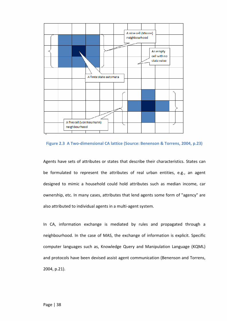
Page | 38

Figure 2.3 A Two-dimensional CA lattice (Source: Benenson & Torrens, 2004, p.23)

Agents have sets of attributes or states that describe their characteristics. States can

be formulated to represent the attributes of real urban entities, e.g., an agent

designed to mimic a household could hold attributes such as median income, car

ownership, etc. In many cases, attributes that lend agents some form of "agency" are

also attributed to individual agents in a multi-agent system.

In CA, information exchange is mediated by rules and propagated through a

neighbourhood. In the case of MAS, the exchange of information is explicit. Specific

computer languages such as, Knowledge Query and Manipulation Language (KQML)

and protocols have been devised assist agent communication (Benenson and Torrens,

2004, p.21).

Page | 39

Due to the sensitivity of raster CA to cell size and neighbourhood configuration

Moreno, Wang, and Marceau (2009) developed a vector based CA (VCA) to overcome

the scale of sensitivity. In VCA space is represented as a collection of interconnected

irregular geographic objects, corresponding to real-world entities, and neighbourhood

is defined as an external buffer around each geographic object that represents an

influenced area. The shape and area of the geographic objects change through time

according to a transition function that incorporates the influence of the neighbours on

the specific geographic object. Its application and results showed that vector based CA

could produce realistic spatial patterns similar referenced LUC maps (Moreno et al.,

2009; Shiyuan & Deren, 2004). Though the VCA seeks to overcome some of the

limitations of raster base CA it has some limitations as well. Moreno et al. (2009 p.53)

concluded that VCA models “still suffer some limitations, including a rigid and

oversimplified definition of the objects and their neighbourhood based on topology,

and the lack of a dynamic representation of the geometry of the objects”. Also the

authors further stated VCA is computational intensive, their work considered three

LUC and used about 48hrs for three iterations. Therefore for complex LUCC model with

higher number of iterations (i.e.: 18 iterations) VCA will not be the most suitable

approach. In view of the limitations and computational intensity of VCA it was not

suitable for this work in modelling dynamic and complex LUCC model.

The Recursive Porous Agent Simulation Toolkit commonly known as RePast (North et

al., 2013) is an example of one of the many MAS tools available. Repast allows for the

implementation of both classical cellular automata, vector based cellular automata

and Agent-based cellular automata. Repast supports the integration of cellular

automata with ESRI Arc Map thereby providing GIS capabilities. However the focus of

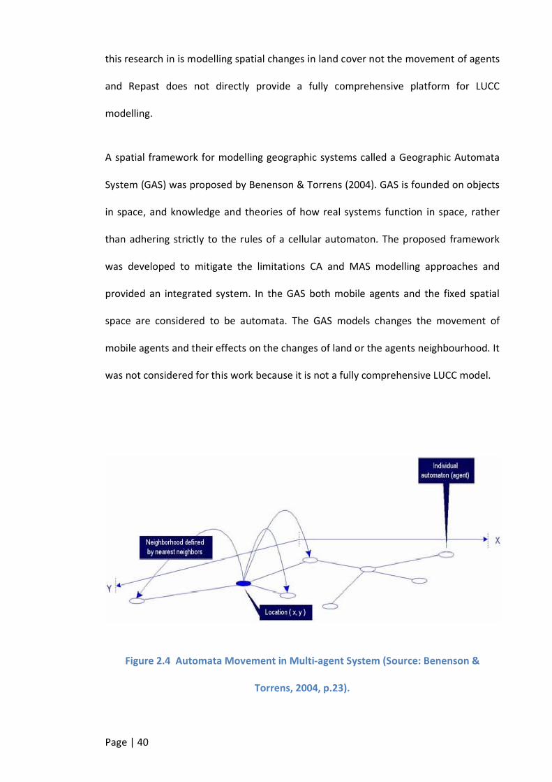
Page | 40

this research in is modelling spatial changes in land cover not the movement of agents

and Repast does not directly provide a fully comprehensive platform for LUCC

modelling.

A spatial framework for modelling geographic systems called a Geographic Automata

System (GAS) was proposed by Benenson & Torrens (2004). GAS is founded on objects

in space, and knowledge and theories of how real systems function in space, rather

than adhering strictly to the rules of a cellular automaton. The proposed framework

was developed to mitigate the limitations CA and MAS modelling approaches and

provided an integrated system. In the GAS both mobile agents and the fixed spatial

space are considered to be automata. The GAS models changes the movement of

mobile agents and their effects on the changes of land or the agents neighbourhood. It

was not considered for this work because it is not a fully comprehensive LUCC model.

Figure 2.4 Automata Movement in Multi-agent System (Source: Benenson &

Torrens, 2004, p.23).

Page | 41

Of the three modelling techniques discussed in section 2.8.1 a hybrid of Cellular

Automata (CA) modelling and statistical/algebraic techniques was considered to be

the most suitable one for this research. The reason is that ABM simulates the mobility

of agents, such as, humans and this research seek to visualise the changes on the

landscape which CA simulates better. Also CA represents and displays/depicts space

and resolution of the landscape better than ABM. The RS LUC data is grid based/raster

data, this makes it more suitable for CA because CA has affinity for gridded data.

Couclelis, (2001), who has almost 30 years’ experience in LUCC modelling, states that

“CA may be seen as a spatial array of ABM” and that though “some researchers

consider mobility to be the defining difference between the two kinds of models, in

reality CA simulates movement in the same way your computer screen does, by

spreading activation down a sequence of adjacent cells or pixels.”

During the calibration phase of this work, the statistical/algebraic technique will be

used in determining the transition rules for the CA engine in the LUCC model.

2.9 Cellular Automata LUCC Models

Although there has been dozens of CA models developed over the years (for example

see: Dietzel & Clarke, 2007; Huang, Zhang, & Lu, 2008; N, Sawant, & Kumar, 2011; Silva

& Clarke, 2002; Soares-Filho, Coutinho Cerqueira, & Lopes Pennachin, 2002), to date

only a few CA-based models are operational as productive tools to support regional

planning practices. Most of these models integrate RS and GIS with CA, using RS and

GIS for the data preparation and visualisation engine. In this section, an overview into

the operational CA models and their workflow process is provided with suggestions for

a generic framework for LUCC modelling.

Page | 42

Researchers have (Clarke, 2012; Lavalle, Barredo, Petrov, Sagris, & Genovese, 2005;

Sun et al., 2009) indicated that to design and develop useful functional models,

designers/modellers must experiment with loosening the constraints of CA and

extending the concept of CA, and also consider integrating a variety of models, such as

socioeconomic, regional and traditional models.

“For land development, the cellular space is a grid of cells representing land parcels

(unit for land development and land use analysis). Cell state describes the

development status of a piece of land. Transition rule is a function that maps the state

of a cell into a new state based on certain conditions that are embedded in the

relationships between the cell and its neighbourhood. CA models articulate a concern

that systems are driven from the bottom up, in which local rules generate global

patterns.” (Hu and Xie, 2006, p. 2)

Models of micro-macro dynamics based on the bifurcation paradigm have helped

modellers in gaining some deep insights into the behaviour of complex systems,

including land development systems. An alternative framework which was developed

using cellular automata depicts an evolution of large scale urban residential areas

represented as the result of a large number of interdependent investment decisions

made by each developer. The exact relation of this model with bifurcation of the same

process remains an interesting theoretical question (Couclelis, 1987).

According to Mount et al. (2008), one of the operational models is the Land-use

Evolution and Impact Assessment Model (LEAM). The LEAM developers aim was to,

design a planning support tool that is focused on land use change which incorporated

recent progress in complex systems analysis techniques, ecological modelling

Page | 43

concepts, geographic spatial analysis, and cellular automata modelling (Sun et al.,

2009).

Figure 2.5 LEAM Framework (Source: Sun et al., 2009).

LEAM consists of two major parts in the framework (Figure 2.5), a land-use change

(LUC) model and an urbanization impact model (Sun et al., 2009). The LUCC model is at

the core of LEAM and helps modellers generate answers to questions such as: How

does land use change under certain assumptions and policies? The second part is the

impact models and it aids in a further interpretation and analysis of urban land-use

change and answers these questions: What does the resultant land-use change pattern

mean? How does it affect water quality, air quality, traffic pattern, and property value,

Page | 44

etc.? Apart from these two views a hidden aspect exists involving dialogue, with

planners and policy makers, which completes the workflow in a feedback cycle. This

third aspect of feedback is very import to LEAM as a planning support tool. Basically, it

asks planners these questions: are the land use change patterns observed within your

evaluation criteria or expect outcomes/targets? If not, how should policies or decisions

be revised, what are the alternatives? In principle these answers from planners are

then used as the feedback input for running another iteration of the LUC scenario (Sun

et al., 2009).

In LEAM conceptually, the surface of the CA on which the cells evolve is constrained

and is defined by factors such as, hydrology, soil, landform and geology. There are also

some socioeconomic factors involved, such as census district and administrative

boundary. Sun et al. (2009, p.60) suggest that for this reason, “the probability of each

cell change is not only decided by the local interactions of neighbour cells, but also by

global information. Therefore, cells in LEAM are intelligent agents that not only can get

the local information, but also can sense the regional or global information, such as

social environment and economic trends.” While most models are free or available to

the public for research the LEAM is only available to research in the LEAM lab.

The Project Gigalopolis led by Clarke (1996) resulted in the SLEUTH model. The name

SLEUTH was derived from the model input data – Slope, Land cover, Exclusion,

Urbanization, Transportation, and Hillshade. It is a combination of the Land Cover

Deltatron Model (LCD) and Urban Growth Model (UGM). Both models LCD and UGM

use CA for modelling and therefore SLEUTH also primarily uses CA to model the

landscape. The work reported to date indicates that SLEUTH has mainly been used for

modelling urban growth and its effects on the land cover or landscape when enabling

Page | 45

the simulation and prediction of land cover or urban growth (Dietzel and Clarke, 2007;

Huang et al., 2008; Leão et al., 2004; Liu and Andersson, 2004; Lakshmi et al., 2011; Yin

et al., 2008)

The main purpose of SLEUTH was to model major USA cities – Detroit, Chicago, New

York, Washington, San Francisco and Albuquerque – and to provide a tool for raising

public awareness of rapid urbanization, that would allow stakeholders to anticipate

and forecast future changes and trends (Lakshmi et al., 2011) . Current research shows

that SLEUTH has been widely used for modelling major cities across the world –

Netherlands, Porte and Lisbon in Portugal, Mexico City in Mexico, Yaoundé in

Cameroun and Sydney in Australia (Clarke, 2012). Thus SLEUTH has been calibrated for

many cities globally, Silva and Clarke (2002) showed greater details of the calibration

of the model to Lisbon and Porto. The following four major findings were presented:

1. SLEUTH is a universal portable model that can not only be applied to USA cities

but to other cities internationally as well.

2. SLEUTH becomes more sensitive to local conditions when the spatial resolution

and detail of the input datasets are increased.

3. using a multi stage Monte Carlo calibration method can better refine the model

parameters to find those that best replicate the historical growth patterns of an

urban system; and

4. the parameters derived from model calibration can be compared between

different systems and the interpretation can provide the foundation for

understanding the urban growth processes unique to each urban system.

Page | 46

The “Modelling of Land Use/Cover Dynamics” (MOLAND) Project (Lavalle et al., 2005)

is an urban modelling tool developed by Research Institute of Knowledge Systems

(RIKS) for the European Commission of Joint Research (JRC), Institute of Environment

and Sustainability (IES). According to IES one of the most potentially useful aspects of

MOLAND is the capacity to simulate future urban and regional growth. The model is

based on a spatial dynamics system and CA. It takes as input five different types of

spatially referenced digital data for the study area: actual land use types; accessibility

of the area to the transport network; inherent suitability of the area for different land

uses; socioeconomic characteristics (population, income, production, employment) of

the area. The model is able to project the likely future development of land use, for

each year for the next 10 to 25 years, based on alternative spatial planning and policy

scenarios.

Most working LUCC models were designed and developed for a specific situation or

location with specific variables (driving factors), because of this modellers do not have

full control on determining the parameters causing LUCC and or fine tuning the models

which mean the models are essentially a “black box”. For MOLAND and LEAM, like

many LUCC working models, modellers do not have access to the source code and

therefore cannot determine or control the parameters but the source code of SLEUTH

is available and modellers have some control over the parameter but not full control.

Because of the lack of flexibility of existing systems a model or a platform that gives

modellers full control over their model will help modellers because the driving forces

of change are not the same in every location. Modellers should be able to decide on

the number of classes of LUC data and determine the adequacy or significance the

variables/parameters before they are included in the LUCC model. For such new

Page | 47

research methods, tools and theory, modellers of ecological systems could potentially

make major improvements to the dynamic changes in physical landscape. “A variety of

sophisticated computational and theoretical tools exist for characterizing urban

systems at a conceptual level, and for visualizing and understanding these

characterizations” (Sun et al., 2009, p. 58).

The development of a comprehensive generic landscape simulation model requires

collaboration between scientists from multiple and diverse disciplines. Guizani et al.

(2010) suggested that, conventional methods of modelling an intricate

multidisciplinary system or unit demand one or more programmers to program

substantive contextual models developed by others. The programmers are tasked with

the separation of the modellers from the original model implementation and these

scientists are the ones who are in a better position to understand the base

composition of the whole model (Guizani et al., 2010).

In traditional methods, the process of model formulation, calibration, coding and

integration are time-consuming and error-prone “The entire model ends up as a black-

box system to users, including the model developers. It is extremely hard to use and

maintain” (Sun et al., 2009).

Due to the problems described above, there is a need to develop another model or

platform using an alternative format. The new strategy should be characterized by two

key differences from the current set of approaches: Firstly, this alternative strategy

must to involve a generic model building environment rather than a black box;

secondly, it should allow for a disaggregated and distributed model integrating

features developed by various subject experts. A generic model building environment

Page | 48

would allow for model parameters and drivers to be easily inspected and evaluated.

Disaggregated and distributed model building would ensure that groups of experts

could work directly on parts of the model with which they were most familiar (Sun et

al., 2009).

Due to the increased complexities in the issues involving contemporary LUC and the

importance placed upon multi-functional LUC in sustainable LUC development is

concerned, researchers are increasingly becoming aware of the need and significance

of studying both the human processes and also the physical processes that cause for

reshaping our LUC. There are two types of approaches which are used in the study of

these processes and the approaches are derived from the natural and social sciences

(Mimler and Priess, 2008; Pimentel and Vassiliadis, 2004).

Multi-disciplinary studies have been identified as a necessity when researching

complex landscape issues. In addition the concept of holism in this approach provides

the opportunity to increase collaboration between different approaches in such a way

that the human and physical dimensions of landscapes may be treated with the same

degree of consideration and in a dynamic way (Ruiz & Domon, 2005).

The Centro de Sensoriamento Remoto (Centre for Remote Sensing) of the

Universidade Federal de Minas Gerais (UFMG), Brazil has developed a CA modelling

platform or software known as DINAMICA EGO (Soares-Filho, 2012). EGO stands for

Environment for Geoprocessing Objects. The software consists of a more advanced or

sophisticated platform for environmental modelling with outstanding possibilities for

the design from the very simple static spatial model to very complex dynamic ones,

which could include nested iterations, multi-transitions, dynamic feedbacks, multi-

Page | 49

region and multi-scale approach decision processes for bifurcating and joining

execution pipelines, and a series of complex spatial algorithms for the analysis and

simulation of space-time phenomena (Soares-Filho, 2012).

DINAMICA EGO simulates landscape or LUC dynamics, using CA, ABM and statistical

approaches to produce the changes in spatial patterns. The major difference between

DINAMICA EGO and other LUCC models is that DINAMICA is not just a model but a

platform. DINAMICA EGO provides modellers tools to model LUCC whilst most of

existing LUCC models (such as SLUETH, LEAM, MOLAND) use a steady scheme with

fixed parameters which could be changed by fine tuning the coefficients to suit a

specific area. Mas et al. (2007) compared selected LUCC models with respect to

amount of change estimated,) allocation of change, reproduction of change pattern,

model validation and advanced simulations and concluded that of the models

evaluated DINAMICA was the most sophisticated m.

For the purpose of the research described in this thesis, the DINAMICA EGO

software/environment will be used to build an LUCC model framework for two study

areas, Auckland Region and Rondônia State, based on the derived workflow process.

Further a vegetative carbon sequestration will be developed as an extension of

Auckland LUCC model to demonstrate that the LUCC model can be used as a

foundation for further studies.

The description of the modelling software environment DINAMICA EGO used for this

research can be found in Appendix 1. The main points worth highlighting are why it is

generic/open modelling software environment, and also how it allows modellers full

control in building models from the beginning to finish. DINAMICA EGO has also has

Page | 50

CA modelling engines, Patcher and Expanders, which are suitable for this research.

DINAMICA take any raster data format input data (Soares-Filho, 2012) . Furthermore

since DINAMICA is not a model but a platform with many tools it should enable the

creation of a unique and complex LUCC model. These are some of the reasons why

DINAMICA was selected for this work.

2.10 Summary

In summary, after reviewing LUCC modelling methods – Statistics, CA and ABM – the

combined method of Statistics and CA was viewed as most appropriate for this work.

Also amongst the LUCC models investigated, SLEUTH and LEAM had the components

to model LUCC but they were closed models not allowing introduction of additional

variables. Their variables influencing change are predefined for all locations thus the

adequacy of such cannot be determined before being introduced into the LUCC model.

DINAMICA EGO modelling environment which uses all the 3 modelling methods (CA,

ABM and statistics) was found to be suitable for the work.

Page | 51

Chapter 3 LUCC Workflow Process Model

This chapter explains the methodology used in designing and implementing a LUCC

model. To inform the development process a candidate area (the Auckland Region)

was selected. The focus for development will be on the workflow process(es) involved

in implementing the LUCC model. As mentioned in section 2.9 the workflow processes

of some models such as SLEUTH, LEAM and MOLAND are specific and closed thus an

open and generic workflow process will be advantage to modellers. One of the major

challenges in developing a successful open and generic model is identifying and

integrating a suitable method for measuring the adequacy and the significance of the

input variables or drivers of LUCC before they are utilised in the modelling process.

Figure 3.1 depicts an integrated workflow process for LUCC modelling from data

preparation through to simulating future scenarios. The calibration processes which

include three processes classification of continuous grey scale variables, computation

of Weights of Evidence of Coefficients and analysis of correlated variables (discussed in

sections 3.3 to 3.5) is designed to help to answer my primary research question: “How

do we determine 'adequacy' when considering the variable and parameter set of

components that describe a LUCC model? What are the measures we can use for this

determination?”

3.1 Data

Data acquisition and preparation for the candidate area is very important in LUCC

modelling. The source, type, resolution and projection of the data will be discussed in

this section. The accuracy of land use cover (LUC) affects the accuracy of LUCC model

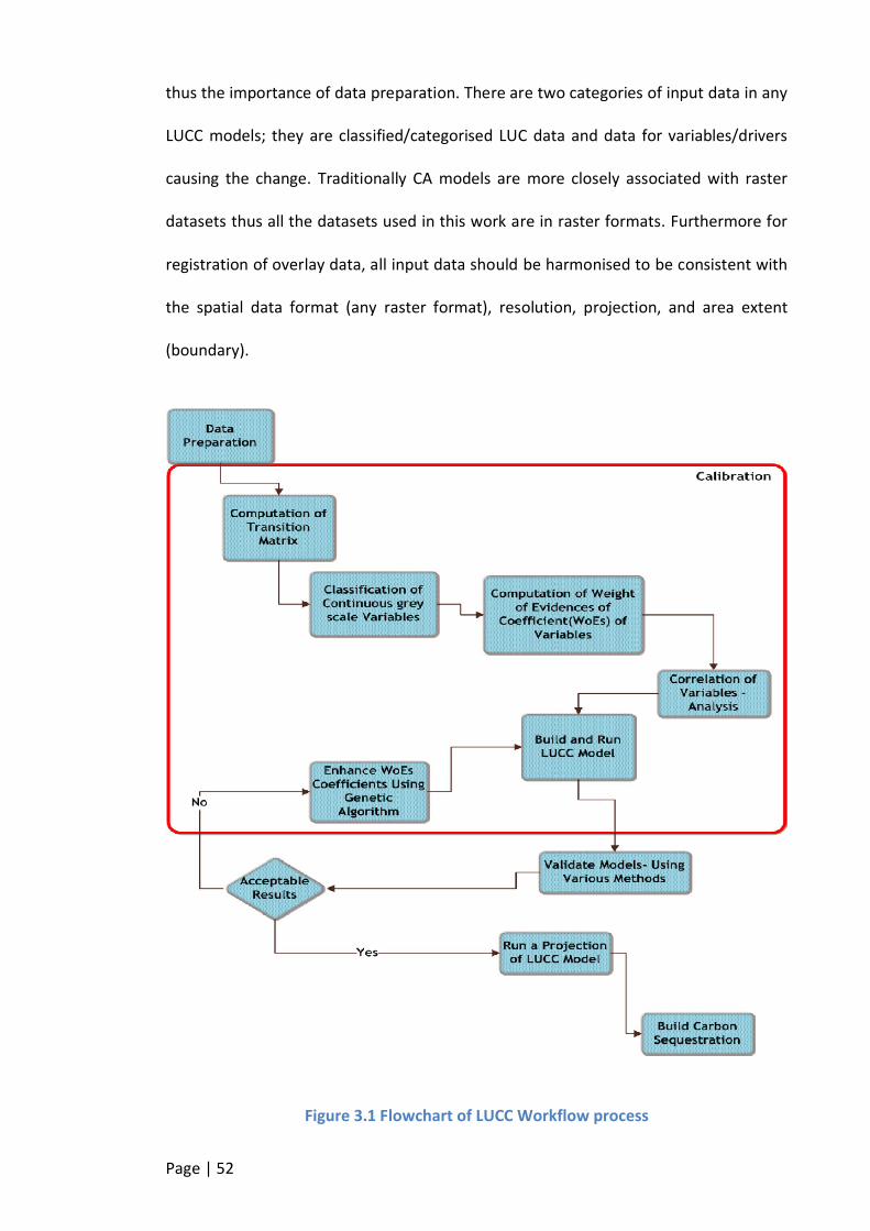
Page | 52

thus the importance of data preparation. There are two categories of input data in any

LUCC models; they are classified/categorised LUC data and data for variables/drivers

causing the change. Traditionally CA models are more closely associated with raster

datasets thus all the datasets used in this work are in raster formats. Furthermore for

registration of overlay data, all input data should be harmonised to be consistent with

the spatial data format (any raster format), resolution, projection, and area extent

(boundary).

Figure 3.1 Flowchart of LUCC Workflow process

Page | 53

The LUC and variable maps used in this work are described in Chapter 6. For each of

the study areas a three LUC maps at different times t1, t2 and t3 were used. The t1

(initial time for the model calibration) and t2 (final time) LUC maps were used for

calibration of model whilst the t3 data was used to validate the model (Clarke, 1996;

Huang et al., 2008; Jantz, Goetz, Donato, & Claggett, 2010; Silva & Clarke, 2002;

Soares-Filho, 2012; Soares-Filho et al., 2002; Sun et al., 2009; Verburg et al., 2006;

Waddell, 2002; Yin et al., 2008). Several variables were tested for “adequacy and

significance” before including them in the model.

3.2 Determination of Transition Matrix

In order to calibrate the LUCC model, the historical context of candidate area should

be analysed within a specific time span, from start time (t1) to end time (t2). The older

LUC map is considered the starting time whilst the recent the end time. In LUCC time

could be defined in units of year, month, or day. The LUC maps are regular lattice of

cells with each cell belonging to a finite set of land use cover classes or states. To

determine a transition matrix, time and land use cover states should be represented by

discrete values.

The transitions between the states of the system are recorded in the form of a

transition matrix that records the probability of moving from one state to another in a

discrete time period. The transition matrix describes a system that changes over

discrete time increments, in which the value of any LUC class or state in a given time

period is the sum of fixed percentages of the value of LUC classes in the previous time

period. The sum of fractions along the row of the transition matrix is equal to one. The

diagonal of the matrix is zero because the cells are unchanged (from = to). The

Page | 54

transition rates are then used in the model as a fixed parameter within a given time

period. A discrete time step can comprise of any time span and this can be set

externally in DINAMICA EGO.

3.2.1 Definitions and Assumptions

The LUCC model uses an overlay of raster maps with each map having the same

number of total cells N. The cells of the LUC maps have the potential of having a finite

number M of different and mutually distinct states and are collectively exhaustive

(which means that the sum of the rows of the probability matrix must be one). Each

cell (i) has a location (x,y); i(x,y), where x,y = 1,2,…, n. Each state of the cell is defined

by an LUC type or class which is within the range k,l = 1,2,…, M; where k is the initial

land use class of cell i at t1 and l is land use class at t2.

Thus, at time t it is assumed that each cell i has only one LUC type k which can be

defined as shown in Eqn 3.1.

��(�) = 1, ��

�(�) = 0, � ≠ �, � = 1,… ,�,��(�) = 1

�

��.�

Where i is the current cell, k is the state of LUC, t is the time and M is the total number

of LUC classes. Thus the definition for the aggregates in terms of cells and or LUC types

may easily be derived from Eqn 3.1 as:

��(�) = ��(�)

�

��.�

�(�) = ��(�)

�

= ��(�)��.�

��

Page | 55

The total number of cells N in the LUCC model is fixed over time, that is

�(�) = �, ��∀�,�ℎ�� = 1,… , �

where τ is the total number of time periods. Although the model allows for

representation of the changes between the total numbers of distinct land use cover

types in cells the total number of aggregate cells of the model is preserved. Therefore

the increase or decrease in a specific land use cover class k can be seen as a transition

from one land use cover class k to another class l. Since each cell is uniform and of the

same size, it is assumed that the density of the cells are the same. Thus the total

density of any land use cover in the system is the proportion of the land use cover to

total aggregate of cells. The density ρk(t) is defined as:

��(�) =��(�)

��.�

The transitional dynamics in the LUCC model may be expressed as the transitions from

one distinct land use cover k at time t to another l at t+1. Thus the transition of cell i

from land use cover k to l could be defined as:

∆�� = 1, �ℎ��

�(�) = 1, ��(� + 1 ) = 1��.�

For the entire system, the aggregate transition from land use cover k to l is expressed

as:

∆�� = ��(� + 1 )

�

−��(�)

�

= ��(� + 1 ) − � �(�) = �∆��

�

��.�

For each land use cover k, the true aggregate change- increment or decrement- is:

Page | 56

∆�� = ��(� + 1 ) − � �(�), �ℎ��∆��

�

= 0��.�

Eqn 3.7 indicates the preservation imposed by having N cells with only one land use

per cell. The model operates from the cellular level to regional, therefore it is

important to take into account transitions at the aggregate level for this helps to

express the long term dynamics of the LUCC model in a simplified way. The total land

use cover l at t+1 can be computed as:

��(� + 1 ) = �∆��

�

��.�

Thus Eqn 3.8 can be expressed in transition probability form as:

��(� + 1 ) = ��(�)

�

��.�

where the probability is expressed as:

�� =∆��

��(�)=

∆��

∑ ∆��

, ��

�

= 1��.��

The process defined, in Eqn 3.8, can be rewritten in matrix-vector form as a first order

Markov chain process, if the probability of each land use cover k or l at time t and t+1

respectively is defined as:

��(�) =��(�)

�, ��(� + 1 ) =

��(� + 1 )

��.��

Page | 57

Thus from the above equations the land use cover l at t+1 is a function of k at t, that is,

�� = �(��) from definitions in Eqn 3.11, Eqn 3.8 can be rewritten as :

�(� + 1 ) = �(�)��.��

Assuming, the transition probabilities are constant and the conditions of connectivity

in the matrix P are relatively weak, then the limit of Eqn 3.12 will lead to

�(� + �) = �(�)��, ��

From Eqn 3.13, as � approaches the limit, then �� → � and Eqn 3.13 gives the steady

state probabilities �as� = �� (de Almeida et al., 2003).

Eqn 3.13 has the structure of a Markovian chain process (Eastman, 2003; Weng, 2002),

where �(�) is a vector with Mx1 dimension (where M is the total number of states, in

this case land use cover classes), �(� + 1 ) is also an Mx1 dimension vector of the

number of LUC states at time t+1 and an MxM matrix of transition probability ��

which executes the probability of transition between each pair of land use covers, k

and l. Thus the transition is expressed as:

⎣⎢⎢⎢⎡123⋮�⎦⎥⎥⎥⎤

��

=

⎣⎢⎢⎢⎡�� … �� … �� … ��⋮ ⋮ ⋮ ⋱ ⋮�� ⋯ ��⎦

⎥⎥⎥⎤�

∗

⎣⎢⎢⎢⎡123⋮�⎦⎥⎥⎥⎤

�

��.��

where k,l = 1, … M and v is the time steps

In DINAMICA EGO the diagonal values of the transition matrix are not used in the

model because there is no change in the cell state. DINAMICA EGO allows for single-

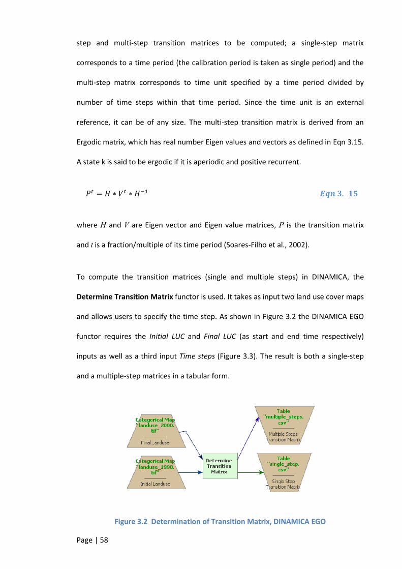
Page | 58

step and multi-step transition matrices to be computed; a single-step matrix

corresponds to a time period (the calibration period is taken as single period) and the

multi-step matrix corresponds to time unit specified by a time period divided by

number of time steps within that time period. Since the time unit is an external

reference, it can be of any size. The multi-step transition matrix is derived from an

Ergodic matrix, which has real number Eigen values and vectors as defined in Eqn 3.15.

A state k is said to be ergodic if it is aperiodic and positive recurrent.

�� = � ∗ �� ∗ ��.��

where H and V are Eigen vector and Eigen value matrices, P is the transition matrix

and t is a fraction/multiple of its time period (Soares-Filho et al., 2002).

To compute the transition matrices (single and multiple steps) in DINAMICA, the

Determine Transition Matrix functor is used. It takes as input two land use cover maps

and allows users to specify the time step. As shown in Figure 3.2 the DINAMICA EGO

functor requires the Initial LUC and Final LUC (as start and end time respectively)

inputs as well as a third input Time steps (Figure 3.3). The result is both a single-step

and a multiple-step matrices in a tabular form.

Figure 3.2 Determination of Transition Matrix, DINAMICA EGO

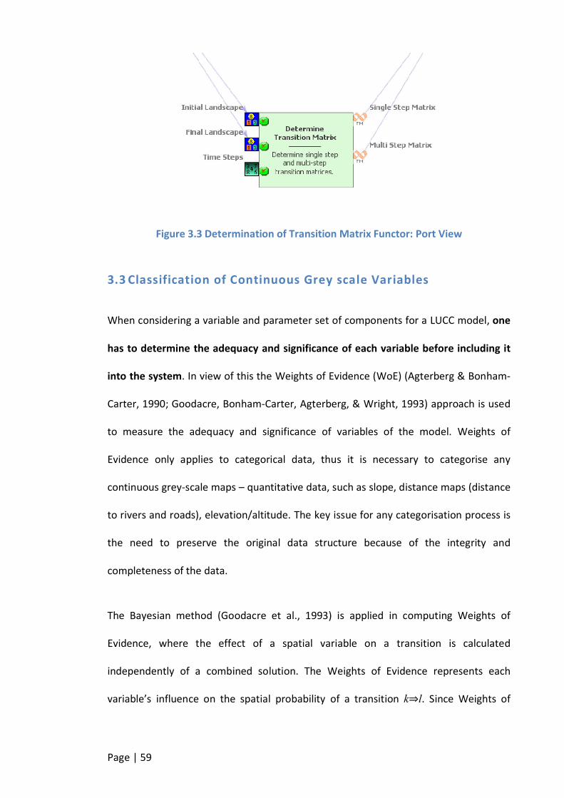
Page | 59

Figure 3.3 Determination of Transition Matrix Functor: Port View

3.3 Classification of Continuous Grey scale Variables

When considering a variable and parameter set of components for a LUCC model, one

has to determine the adequacy and significance of each variable before including it

into the system. In view of this the Weights of Evidence (WoE) (Agterberg & Bonham-

Carter, 1990; Goodacre, Bonham-Carter, Agterberg, & Wright, 1993) approach is used

to measure the adequacy and significance of variables of the model. Weights of

Evidence only applies to categorical data, thus it is necessary to categorise any

continuous grey-scale maps – quantitative data, such as slope, distance maps (distance

to rivers and roads), elevation/altitude. The key issue for any categorisation process is

the need to preserve the original data structure because of the integrity and

completeness of the data.

The Bayesian method (Goodacre et al., 1993) is applied in computing Weights of

Evidence, where the effect of a spatial variable on a transition is calculated

independently of a combined solution. The Weights of Evidence represents each

variable’s influence on the spatial probability of a transition k⇒l. Since Weights of

Page | 60

Evidence is the core approach I used in calibrating the LUCC I seek to discuss the

assumptions and definitions used to derive the WoE in Section 3.3.1.

3.3.1 Definitions and Assumptions: Weights of Evidence

Given a binary map of spatial pattern, B (defining the presence or absence of spatial

pattern) and a map of events D, such as land use cover change, the weighting factors

W+ and W- can be calculated from the ratios of conditional probabilities and may be

stated as follows :

�� = �� (�|�)

�(�|��)� �� = ��

�(��|�)

�(��|��)� ��.��

where B and �� stand for the presence and absence of binary spatial map pattern

respectively and, D and �� stand for presence and absence of land use cover change

event respectively (Agterberg & Bonham-Carter, 1990; Goodacre, Bonham-Carter,

Agterberg & Wright, 1993). The contrast, C, is a measure of the spatial association

between the binary pattern and the events is given by

� =�� −� ��.��

To give an example, suppose we took all of the black pieces of a chess set and arranged

them on a chess board. If all of the black pieces are placed on black squares, the

contrast would be positive, if all the pieces are on white squares the contrast would be

negative and if half of the pieces were on black squares and the other half on white

squares, the contrast would be zero.

Page | 61

To determine whether the magnitude of the contrast is good enough to be statistically

significant variance of the contrast s2(C) can be used and can be expressed as:

��(�) =1

��(� ∩ �)+

1

��(� ∩ ��)+

1

��(�� ∩ �)+

1

��(�� ∩ ��)��.��

The contrast(C) indicating whether or not there is a relationship between B and D is

said to be statistically significant with 95% probability if |C| > 1.96 s(C).

The conditional probabilities used in these formulae are determined by measuring the

overlapping areas between D and B where:

�(�|�) =��(�∩�)

��(�)��.��b

is the conditional probability that a land use cover change event intersects with the

binary pattern; in determination of this the ratio requires the measurement of

i) the area where events occur on the binary pattern (the intersection), and

ii) the total area occupied by all events.

For cases where the events occur on the binary spatial pattern more frequently than

anticipated W+ will be positive and W- will be negative, and the value or extent of the

contrast, C, reflects the whole spatial relationship of the events with the binary

pattern.

The likelihood of an event D occurring in a spatial pattern B, can be expressed by the

conditional or posterior probability (Eqn 3.19).

Page | 62

�{�|�} =�{� ∩ �}

�{�}��.��

where D is number of cells in a raster map and overlap with B as

�{� ∩ �} =��(� ∩ �)

��.��

a fraction of the area occupied by B or D with respect to the entire area A is given as

�{�} =�

�,��{�} =

�

��.��

In representing the conditional probability in terms of its odds as�{�|�}

��{�|�}, if (��)

represents the absence of (D) and O{D} represents the prior odds ratio of event (D)

then

�{�} =�{�}

�{��},�ℎ��{�|�} =

�{�|�}

�{��|�}��.��

Then

��{�|�} = ��{�} +� ��.��

where W+ is the Weight of Evidence of event D occurring, given a spatial pattern B,

then the post probability of a transition k⇒l given a set of spatial data (B, C, D,... N) is

expressed as follows:

�{� ⇒ �|� ∩ � ∩ �…∩ �} =�∑ ��

�

��∑ ��

� ��.��

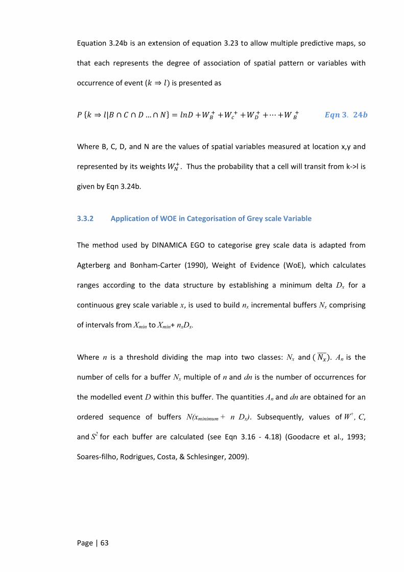
Page | 63

Equation 3.24b is an extension of equation 3.23 to allow multiple predictive maps, so

that each represents the degree of association of spatial pattern or variables with

occurrence of event (� ⇒ �) is presented as

�{� ⇒ �|� ∩ � ∩ �…∩ �} = �� +�� + ��

� + �� + ⋯+��

��.��

Where B, C, D, and N are the values of spatial variables measured at location x,y and

represented by its weights ��. Thus the probability that a cell will transit from k->l is

given by Eqn 3.24b.

3.3.2 Application of WOE in Categorisation of Grey scale Variable

The method used by DINAMICA EGO to categorise grey scale data is adapted from

Agterberg and Bonham-Carter (1990), Weight of Evidence (WoE), which calculates

ranges according to the data structure by establishing a minimum delta Dx for a

continuous grey scale variable x, is used to build nx incremental buffers Nx comprising

of intervals from Xmin to Xmin+ nxDx.

Where n is a threshold dividing the map into two classes: Nx and (��). An is the

number of cells for a buffer Nx multiple of n and dn is the number of occurrences for

the modelled event D within this buffer. The quantities An and dn are obtained for an

ordered sequence of buffers N(xminimum + n Dx). Subsequently, values of W+, C,

and S2 for each buffer are calculated (see Eqn 3.16 - 4.18) (Goodacre et al., 1993;

Soares-filho, Rodrigues, Costa, & Schlesinger, 2009).

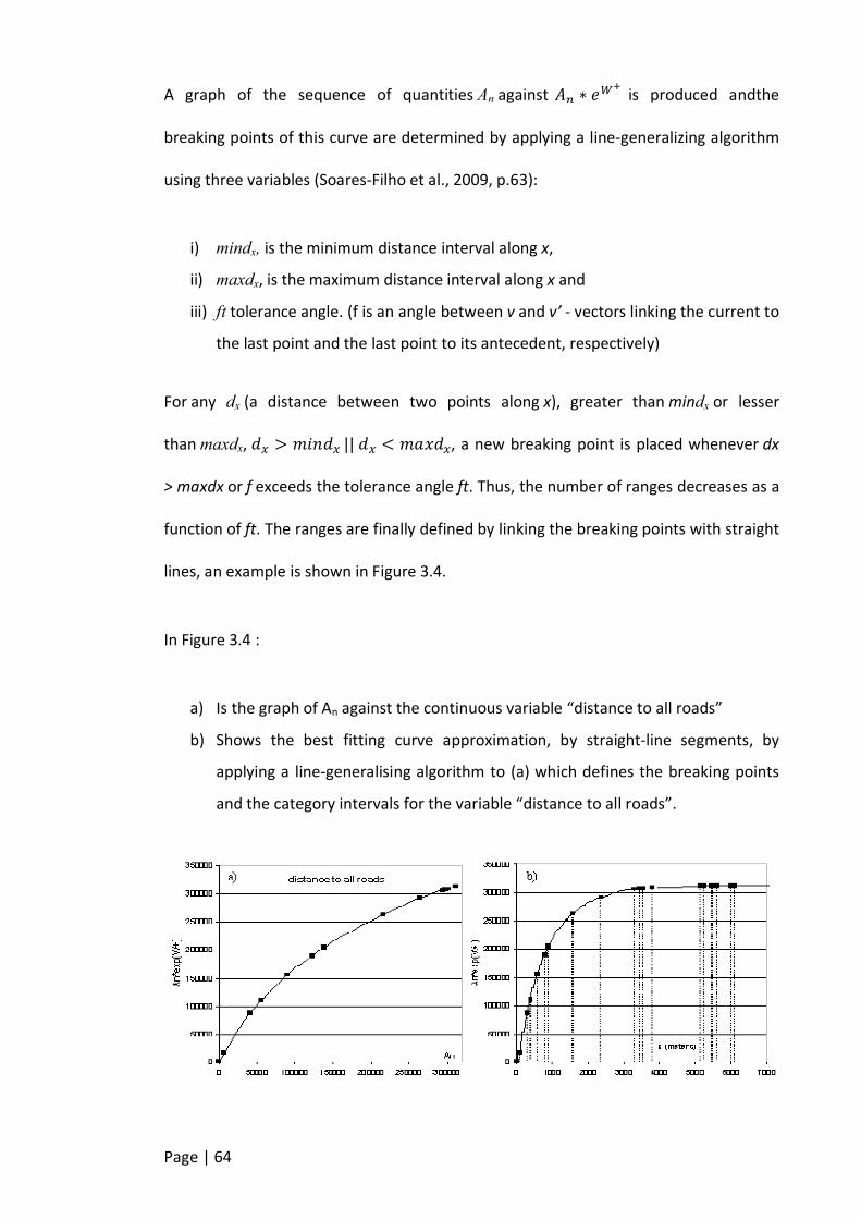
Page | 64

A graph of the sequence of quantities An against �� ∗ �� is produced andthe

breaking points of this curve are determined by applying a line-generalizing algorithm

using three variables (Soares-Filho et al., 2009, p.63):

i) mindx, is the minimum distance interval along x,

ii) maxdx, is the maximum distance interval along x and

iii) ft tolerance angle. (f is an angle between v and v’ - vectors linking the current to

the last point and the last point to its antecedent, respectively)

For any dx (a distance between two points along x), greater than mindx or lesser

than maxdx, �� > ��||�� < ��, a new breaking point is placed whenever dx

> maxdx or f exceeds the tolerance angle ft. Thus, the number of ranges decreases as a

function of ft. The ranges are finally defined by linking the breaking points with straight

lines, an example is shown in Figure 3.4.

In Figure 3.4 :

a) Is the graph of An against the continuous variable “distance to all roads”

b) Shows the best fitting curve approximation, by straight-line segments, by

applying a line-generalising algorithm to (a) which defines the breaking points

and the category intervals for the variable “distance to all roads”.

Page | 65

Figure 3.4 Graph showing Breakpoints based on the Grey Scale Variable

The implementation of the Categorisation of Continuous Grey-scale variable in

DINAMICA EGO, employs the functor Weights of Evidence of Ranges as shown in

Figure 3.6 and Figure 3.5. In Figure 3.6:

the event or transition ( � ⇒ � where k is the initial land use cover and l the

land use cover a cell has transited to) is selected, and

the continuous grey scale variable to be categorised in relation to the event is

also selected.

user inputs the following variables

o of increment dx,

o minimum (mindx) and maximum(maxdx) delta, and

o tolerance angel ft

3.4 Computation of the WoE Coefficients of Variables

Based on the definitions and assumptions of Weights of Evidence as discussed in

section 3.3.1, the Weights of Evidence Coefficients of variables causing change in an

event D (where D is the change from land use cover class k to land use class l) can be

computed.

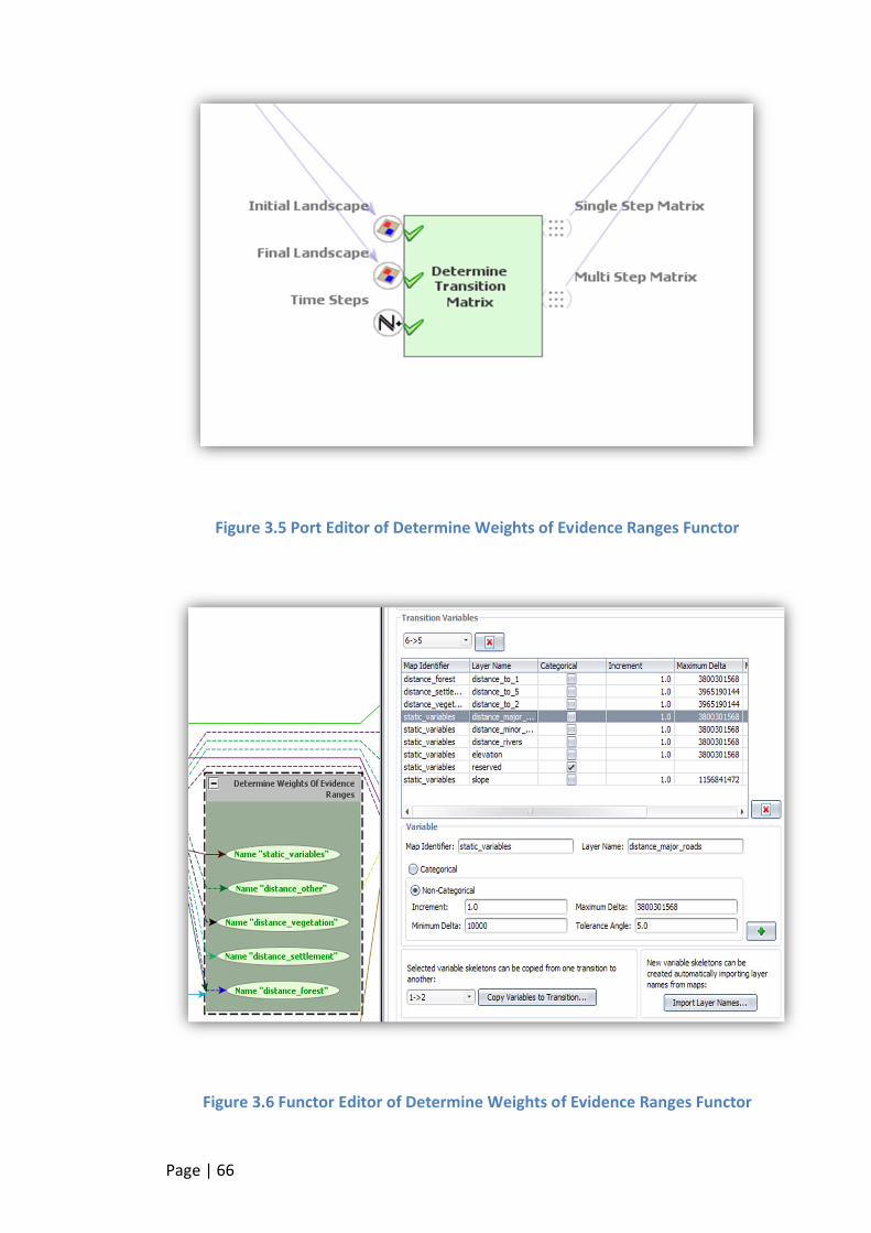
Page | 66

Figure 3.5 Port Editor of Determine Weights of Evidence Ranges Functor

Figure 3.6 Functor Editor of Determine Weights of Evidence Ranges Functor

Page | 67

This calibration phase is important in LUCC modelling because every variable which is

introduced into the model should have a scientific basis for its inclusion (does the

variable influence a change? and if it does what is the measure?). It is worth noting

that a variable might cause a change in one event and not influence change in other

events, for example the variable distance to roads may be significant in the change

from vegetation to settlements but may not cause change in all the other transitions in

the same LUCC. Thus it is important to determine the Weights of Evidence of

Coefficients for variables in each transitional event.

For the computation of Weights of Evidence (WoE) Coefficients of variables,

all variables anticipated to cause transitional change, are categorised into

ranges

the ranges are specific for every transition, such that for each transition there is

a new categorisation of the variable.

WoE coefficients are assigned to a range of values for the variable, which

determines the influence of change of the variable within each range for a

specific transition.

Figure 3.7 presents a sample of the WoE coefficients results, for the candidate area,

the first line represents the variable name with ranges, where 0:1, 1:101, 142:201 are

ranges 0 to 1, 1 to 101, 142 to 201 respectively. The first column of the second line

indicates the transitional event (e.g. 1,2 stands for transition from class 1 to 2) and

subsequent numbers are WoE coefficients corresponding ranges of the variables in the

above line.

Page | 68

Figure 3.7 Sample Results of WoE Coefficients

Figure 3.8 Graphs of WoE vs. Ranges

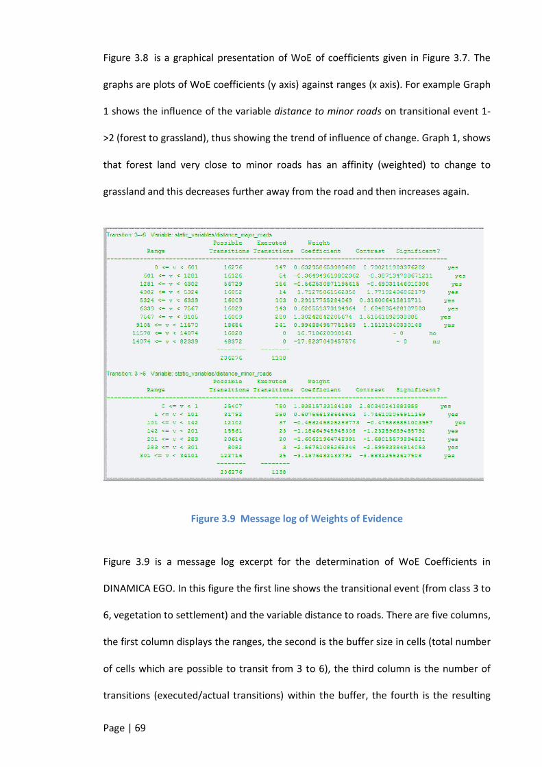
Page | 69

Figure 3.8 is a graphical presentation of WoE of coefficients given in Figure 3.7. The

graphs are plots of WoE coefficients (y axis) against ranges (x axis). For example Graph

1 shows the influence of the variable distance to minor roads on transitional event 1-

>2 (forest to grassland), thus showing the trend of influence of change. Graph 1, shows

that forest land very close to minor roads has an affinity (weighted) to change to

grassland and this decreases further away from the road and then increases again.

Figure 3.9 Message log of Weights of Evidence

Figure 3.9 is a message log excerpt for the determination of WoE Coefficients in

DINAMICA EGO. In this figure the first line shows the transitional event (from class 3 to

6, vegetation to settlement) and the variable distance to roads. There are five columns,

the first column displays the ranges, the second is the buffer size in cells (total number

of cells which are possible to transit from 3 to 6), the third column is the number of

transitions (executed/actual transitions) within the buffer, the fourth is the resulting

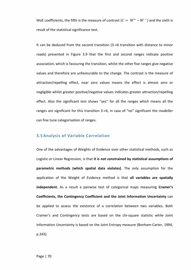
Page | 70

WoE coefficients, the fifth is the measure of contrast (� =�� − � �) and the sixth is

result of the statistical significance test.

It can be deduced from the second transition (3->6 transition with distance to minor

roads) presented in Figure 3.9 that the first and second ranges indicate positive

association, which is favouring the transition, whilst the other five ranges give negative

values and therefore are unfavourable to the change. The contrast is the measure of

attraction/repelling effect, near zero values means the effect is almost zero or

negligible whilst greater positive/negative values indicates greater attraction/repelling

effect. Also the significant test shows “yes” for all the ranges which means all the

ranges are significant for this transition 3->6, in case of “no” significant the modeller

can fine tune categorisation of ranges.

3.5 Analysis of Variable Correlation

One of the advantages of Weights of Evidence over other statistical methods, such as

Logistic or Linear Regression, is that it is not constrained by statistical assumptions of

parametric methods (which spatial data violates). The only assumption for the

application of the Weight of Evidence method is that all variables are spatially

independent. As a result a pairwise test of categorical maps measuring Cramer’s

Coefficients, the Contingency Coefficient and the Joint Information Uncertainty can

be applied to assess the existence of a correlation between two variables. Both

Cramer’s and Contingency tests are based on the chi-square statistic while Joint

Information Uncertainty is based on the Joint Entropy measure (Bonham-Carter, 1994,

p.243).

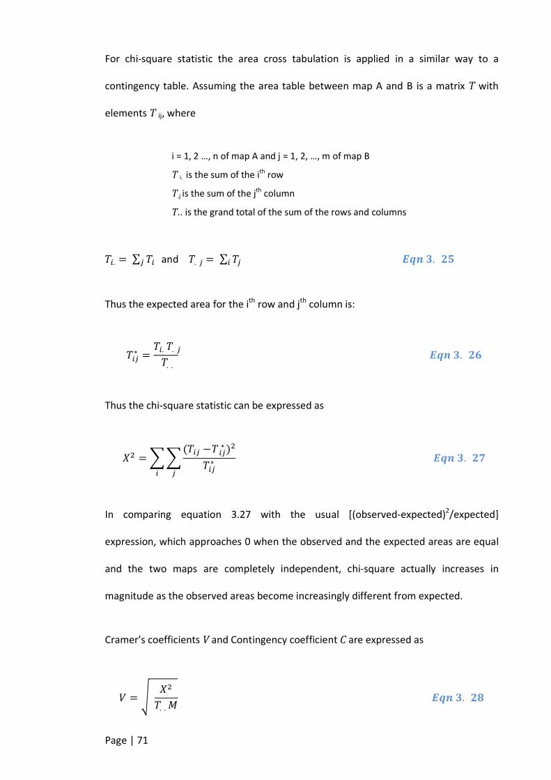
Page | 71

For chi-square statistic the area cross tabulation is applied in a similar way to a

contingency table. Assuming the area table between map A and B is a matrix T with

elements T ij, where

i = 1, 2 …, n of map A and j = 1, 2, …, m of map B

T i. is the sum of the ith row

T.j is the sum of the jth column

T.. is the grand total of the sum of the rows and columns

��.= ∑ �� and �.�= ∑ �� .��

Thus the expected area for the ith row and jth column is:

��∗ =

��.�.��..

��.��

Thus the chi-square statistic can be expressed as

�� = ��(�� − ��

∗ )�

��∗

��

��.��

In comparing equation 3.27 with the usual [(observed-expected)2/expected]

expression, which approaches 0 when the observed and the expected areas are equal

and the two maps are completely independent, chi-square actually increases in

magnitude as the observed areas become increasingly different from expected.

Cramer’s coefficients V and Contingency coefficient C are expressed as

� = ��

�..��.��

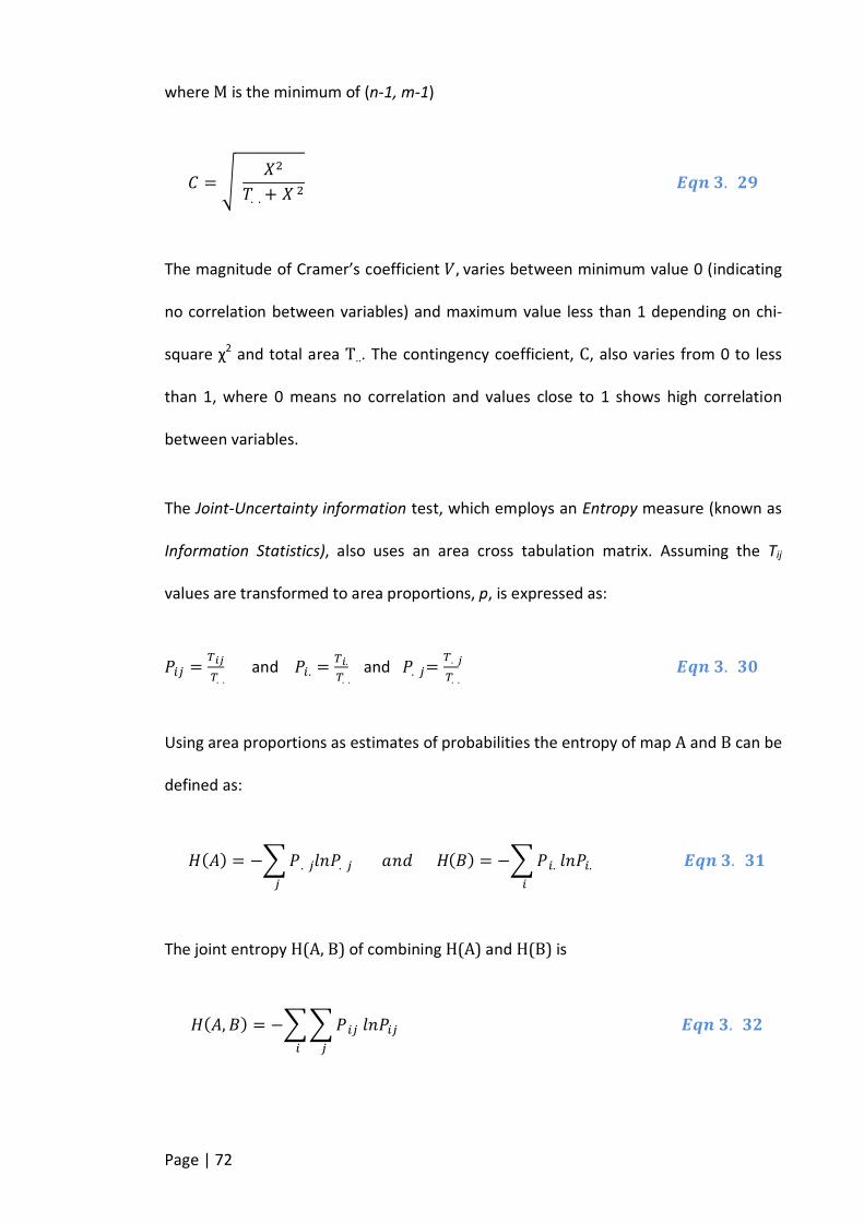
Page | 72

where M is the minimum of (n-1, m-1)

� = ��

�..+ � ��.��

The magnitude of Cramer’s coefficient �, varies between minimum value 0 (indicating

no correlation between variables) and maximum value less than 1 depending on chi-

square χ2 and total area T... The contingency coefficient, C, also varies from 0 to less

than 1, where 0 means no correlation and values close to 1 shows high correlation

between variables.

The Joint-Uncertainty information test, which employs an Entropy measure (known as

Information Statistics), also uses an area cross tabulation matrix. Assuming the Tij

values are transformed to area proportions, p, is expressed as:

�� =��

�.. and ��.=

��.

�.. and �.�=

�.�

�..��.��

Using area proportions as estimates of probabilities the entropy of map A and B can be

defined as:

�(�) = −��.��.��

��(�) = −��.��.�

��.��

The joint entropy H(A, B) of combining H(A) and H(B) is

�(�, �) = −��

��.��

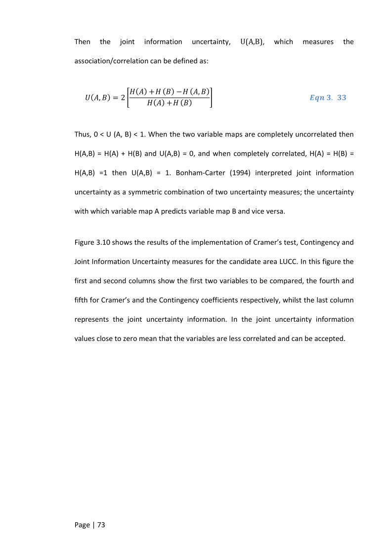
Page | 73

Then the joint information uncertainty, U(A,B), which measures the

association/correlation can be defined as:

�(�, �) = 2��(�) + � (�) − � (�, �)

�(�) + � (�)� ��.��

Thus, 0 < U (A, B) < 1. When the two variable maps are completely uncorrelated then

H(A,B) = H(A) + H(B) and U(A,B) = 0, and when completely correlated, H(A) = H(B) =

H(A,B) =1 then U(A,B) = 1. Bonham-Carter (1994) interpreted joint information

uncertainty as a symmetric combination of two uncertainty measures; the uncertainty

with which variable map A predicts variable map B and vice versa.

Figure 3.10 shows the results of the implementation of Cramer’s test, Contingency and

Joint Information Uncertainty measures for the candidate area LUCC. In this figure the

first and second columns show the first two variables to be compared, the fourth and

fifth for Cramer’s and the Contingency coefficients respectively, whilst the last column

represents the joint uncertainty information. In the joint uncertainty information

values close to zero mean that the variables are less correlated and can be accepted.

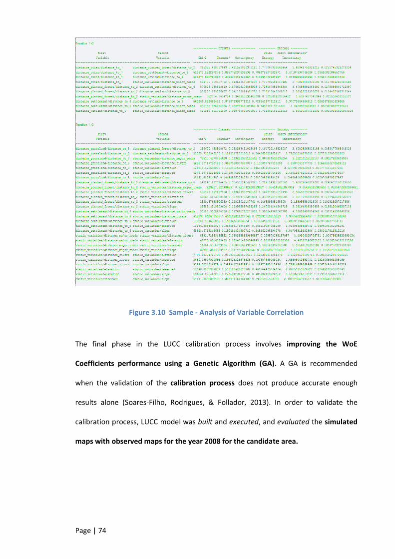
Page | 74

Figure 3.10 Sample - Analysis of Variable Correlation

The final phase in the LUCC calibration process involves improving the WoE

Coefficients performance using a Genetic Algorithm (GA). A GA is recommended

when the validation of the calibration process does not produce accurate enough

results alone (Soares-Filho, Rodrigues, & Follador, 2013). In order to validate the

calibration process, LUCC model was built and executed, and evaluated the simulated

maps with observed maps for the year 2008 for the candidate area.

Page | 75

3.6 Building and Running LUCC Simulation Model

This section describes and explains the integration of the various workflow

processes/phases into a LUCC Simulation Model. The generic modelling environment

and GUI of DINAMICA EGO makes it suitable and easier to integrate the workflow

processes. Figure 3.11 is a DINAMICA EGO diagram showing integration of the

processes of LUCC modelling and Figure 3.12 is the flow chart for LUCC simulation

model which further explains Figure 3.11.

3.6.1 LUCC Model Data

As shown in Figure 3.11 the input data are:

Initial land use cover map

Multiple Transition Matrix

WoE Coefficients of Variables

Static and dynamic variable maps

The variable (driving factors) maps are in two categories, static and dynamic variable

maps. Static variables such as slope, elevation, distance to major and minor roads,

distance to rivers, soil and reserved lands do not change in value through the iteration

process because they are computed only once before running the simulation model.

On the other hand dynamic variables such as distance to land use cover class (e.g.

natural forest, planted forest, crop land, settlement and wetland) are computed

before an iteration thus changing in values after each time step. The variable maps

represent distance from a cell of a particular LUC class cell to the nearest cell of a

different LUC class at a specific time step.

Page | 76

3.6.2 Computation of Spatial Transition Probabilities

The spatial/local transition probabilities are computed for each cell in the LUC map for

every specific transition considering the natural and anthropic state of cells. Using the

WoE method (Eqn 3.16), which employs Eqn 3.24a and 4.24b, the probability of a cell

to transit from land use class k ->l are computed. Using the values of W+ derived from

Eqn 3.16 in 4.24a and 4.24b, the cells’ transition probabilities are computed (Maeda et

al., 2011). Regarding Eqn 3.16 it can be interpreted as, the higher the value of W+ the

greater the probability of that transition to occur compared to other computing

transitions. Thus cells are assigned a value of probability for each transition and

respective probability maps generated. It is worthy of note that the method models

transitions and not the state frequencies.

DINAMICA EGO computes spatial transition probability maps using the functor “Cal W.

OF. E Probability Map” as in Figure 3.11. As an input, the functor uses WoEs of

Coefficients of variables and LUC map at time t.

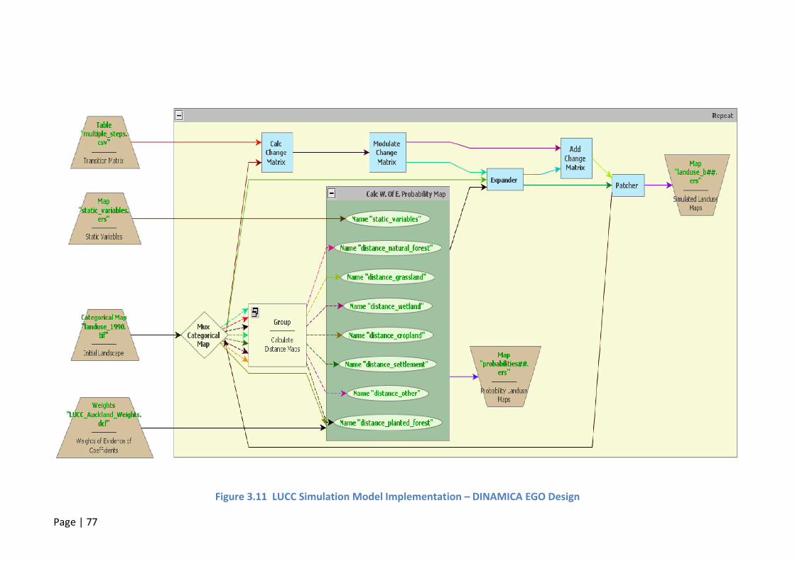
Page | 77

Figure 3.11 LUCC Simulation Model Implementation – DINAMICA EGO Design

Page | 78

Figure 3.12 Flowchart of LUCC Modelling

3.6.3 Allocation of Simulated Land Changes

For CA LUCC modelling, an issue to consider is the influence of neighbourhood cells in

the transition probabilities. DINAMICA EGO uses a local CA transition engine

composed of two complimentary land use transition functions (allocation algorithms),

Expander and Patcher, in dealing with this issue (Soares-Filho et al., 2002). The

Expander is for the expansion or contraction of previous patches of given land use

cover class whilst the Patcher algorithm generates or form new land use cover class

patches through a seeding mechanism. Thus, the Expander algorithm executes

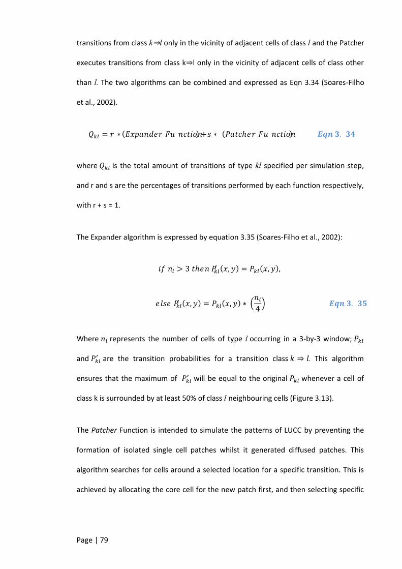
Page | 79

transitions from class k⇒l only in the vicinity of adjacent cells of class l and the Patcher

executes transitions from class k⇒l only in the vicinity of adjacent cells of class other

than l. The two algorithms can be combined and expressed as Eqn 3.34 (Soares-Filho

et al., 2002).

�� = � ∗(��) + � ∗ (��ℎ��)��.��

where �� is the total amount of transitions of type kl specified per simulation step,

and r and s are the percentages of transitions performed by each function respectively,

with r + s = 1.

The Expander algorithm is expressed by equation 3.35 (Soares-Filho et al., 2002):

�� > 3�ℎ�� (�, �) = ��(�, �),

�� (�, �) = ��(�, �) ∗�

��

4� ��.��

Where �� represents the number of cells of type l occurring in a 3-by-3 window;��

and �� are the transition probabilities for a transition class � ⇒ �. This algorithm

ensures that the maximum of �� will be equal to the original �� whenever a cell of

class k is surrounded by at least 50% of class l neighbouring cells (Figure 3.13).

The Patcher Function is intended to simulate the patterns of LUCC by preventing the

formation of isolated single cell patches whilst it generated diffused patches. This

algorithm searches for cells around a selected location for a specific transition. This is

achieved by allocating the core cell for the new patch first, and then selecting specific

Page | 80

number of cells around the core cell according to their Pkl transition probabilities as

illustrated in Figure 3.14.

Figure 3.13 Pkl arrays before [a] and after [b] convolution of Expander (Source :

Soares-Filho et al., 2002, p.23).

Figure 3.14 Generation of Cells around allocated core cell by Patcher

Page | 81

As outlined by Soares-Filho et al. (2002), for each simulation time step the percentages

of transitions are computed and set for each of the functions (Expander and Patcher).

Both transition algorithms employ a stochastic allocation method which is responsible

for finding cells with the highest transition probabilities for each kl transition. The

allocation method stores the cells and sorts them for subsequent selection. With this

method, the newly selected cell becomes the core for a new patch or

expansion/contraction edges which could be developed using transitional functions.

The size of the new patches and expansion/contraction edges are set according to

lognormal probability distribution. It is therefore imperative to set the parameters of

the distribution, mean size and variance size, of each new patch or

expansion/contraction edge to be created.

In DINAMICA EGO (Figure 3.11), the Expander functor is executed first then the

Patcher functor. The Modulate Change Matrix functor (see Eqn 3.34) regulates

(dividing into r and s whereby r + s = 1) the quantity of change per transition between

the Patcher and Expander functions. It is worth noting that in Figure 3.11 the quantity

of change per transitions which are not executed by Expander are then passed onto

the Patcher through the Add Change Matrix functor, to ensure that all the quantities of

change are executed.

3.6.4 Execution Process of the LUCC Simulation Model

This subsection describes the execution of the integrated processes as presented in

Figure 3.11. The LUCC simulation model takes as inputs the results of the following

process:

Computation of Transition Matrix - Multiple Transition Matrix

Page | 82

Computation of Weight of Evidence Coefficients of Variables - WoE Coefficients

of Variables

Data preparation – Static Variables and Land Use Cover Map

Dynamic variables are derived from the initial LUC map through the Mux Categorical

Map and then the various distance maps are computed.

For each sojourn time, Calc Change Matrix computes the amount of change per

transition by multiplying the transition rates (from the multiple transition matrices) by

the number of cells of each land use cover class per each sojourn time (from the

dynamic LUC map of the Mux Categorical Map). The amount of transitional change is

regulated for the Expander and Patcher by the Modulate Change Matrix functor.

The simulation engine of DINAMICA EGO is the Expander and Patcher and employs the

CA modelling approach. The Expander is executed using a percentage of the amount

of change per transition (from the Modulate Change Matrix) and the local transition

probabilities to simulate expansion/contraction of LUC class(es). The changes which

are not executed by Expander are passed onto the Patcher for execution. The

simulated map is saved and at the same time passed to be used as the initial LUC map

(connects to Mux Categorical Map) for the next sojourn time iteration. The Repeat

container (Figure 3.11) handles the number of iterations (time steps), this is entered by

the modeller, and the model generates simulated maps after each iteration.

3.7 Validation of the Simulation Model

The working processes of the spatially-explicit LUCC simulation model begins with a

digital LUC map of an initial time and then simulates transitions in order to generate

Page | 83

simulated/prediction map(s) for subsequent discrete time(s). The obvious questions in

analysing the simulated map are:

How well did the model perform in measuring the prediction accuracy of the

model? (Verburg et al., 2006)

Does the model generate the correct quantity in each LUC class?

Does the model place the specific LUC classes in the correct locations? (Pontius,

2002)

Thus, in LUCC modelling, it is important to validate the model before it is used to build

scenarios. Rykiel(1996, p.5) states that “validation is a demonstration that a model

within its domain of applicability possesses a satisfactory range of accuracy

consistent with the intended application of the model”. Verburg et al. (2006)

asserts that it is not useful to crown a model as valid or to condemn a model as invalid

based on validation results, rather its more useful to state the degree to which the

model is valid. Hence validation in this work measures the performance of the model

to reveal the level of trust or confidence that one should put in the model.

Map comparison is the method most used in validating LUCC models either

qualitatively and or quantitatively (Visser, 2004; Verburg et al., 2006). Map comparison

is a simple comparison of the simulated maps with observed/reference maps to

measure similarity between the two maps. There are numerous mathematical

methods used by LUCC modellers to quantify the similarity of maps such as the cell-by-

cell kappa and fuzzy sets map comparisons (Visser, 2004; Verburg et al., 2006).

For most purposes, a careful visual inspection of maps (reveal many interesting

characteristics) arguably performs better than mathematical procedures in validation

Page | 84

(Visser, 2004). The human observer takes many aspects (such as local similarities,

global similarities, logical coherence and patterns) into consideration when comparing

maps. Map comparison by mathematical procedures usually captures one of these

aspects ignoring the others (Visser, 2004). Despite the rigidity of current mathematical

methods of map comparison, in some circumstances it is preferred to a visual map

comparison, for example for large area maps automated mathematical methods save

time and are likely to be less error prone than human observation.

Figure 3.15 Map Comparison of Checker Boards

An example of the rigidity of mathematical methods is clearly illustrated by a cell-by-

cell comparison of two checker boards as in Figure 3.15 in which it can be observed

that (a) has a white cell at the top left corner whilst (b) has black. A cell-by-cell

comparison method would find a white cell where black cell is expected and vice versa,

however an average human observer would immediately appreciate that (a) and (b)

are very similar qualitatively where a statistical method would only show that they are

significantly different.

Page | 85

An automated map comparison within a neighbourhood context rather than a cell-by-

cell context will be more suitable for LUCC model because a neighbourhood context

considers the similarity in the pattern of change. In an attempt to resolve the issue of

vicinity-based comparison several methods have been developed.

Multiple Fitting Procedure which compares a map fit within increasing window

sizes. This method quantifies the goodness of fit of LUCC models by measuring

the similarity of the patterns at different resolutions in order to describe

complexity of the spatial patterns (Costanza, 1989).

Pontius (2002) introduced a method similar to Multiple Fitting Procedure, but

partitions the overall validation into six as; correct due to chance, correct due

to location, correct due to quantity, error due to location and error due to

quantity.

Power, Simms, and White (2001) presented a combined method of polygon

mapping and hierarchical fuzzy pattern matching to compare maps on both

local and global level.

Hagen (2003) developed a method applying fuzzy set theory (known as kfuzzy

which is kappa statistic and fuzzy similarity), considering the fuzziness of

location and LUC class/category within a cell vicinity. The method produces a

map which specifies the degree of similarity, ranging from 0 to 1, of each cell.

Overall value of similarity if derived from the local spatial assessment of

similarity.

Soares-Filho et al. (2009) modified the method of Hagen (2003) and named it

Reciprocal Similarity, employing exponential decay function using distance to

weight the cell state distribution around the core cell.

Since this work seeks to validate the process of change and not the maps themselves, a

method which considers vicinity is preferred to cell-to-cell method. Also a method

comparing the fitness of the model at different window resolutions will help to reveal

the performance of the model at different resolutions. Thus a combination of

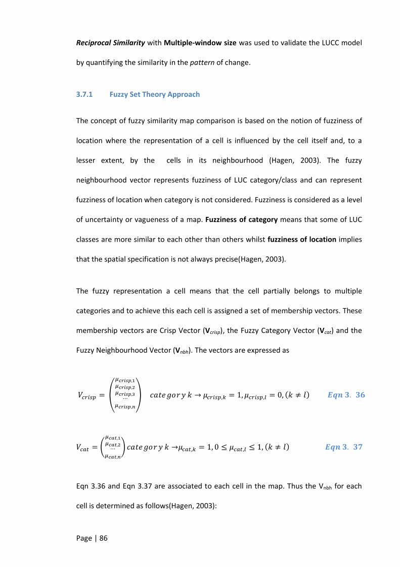
Page | 86

Reciprocal Similarity with Multiple-window size was used to validate the LUCC model

by quantifying the similarity in the pattern of change.

3.7.1 Fuzzy Set Theory Approach

The concept of fuzzy similarity map comparison is based on the notion of fuzziness of

location where the representation of a cell is influenced by the cell itself and, to a

lesser extent, by the cells in its neighbourhood (Hagen, 2003). The fuzzy

neighbourhood vector represents fuzziness of LUC category/class and can represent

fuzziness of location when category is not considered. Fuzziness is considered as a level

of uncertainty or vagueness of a map. Fuzziness of category means that some of LUC

classes are more similar to each other than others whilst fuzziness of location implies

that the spatial specification is not always precise(Hagen, 2003).

The fuzzy representation a cell means that the cell partially belongs to multiple

categories and to achieve this each cell is assigned a set of membership vectors. These

membership vectors are Crisp Vector (Vcrisp), the Fuzzy Category Vector (Vcat) and the

Fuzzy Neighbourhood Vector (Vnbh). The vectors are expressed as

�� = �

��,��,��,�

⋯��,�

� �� → ��,� = 1, ��,� = 0, (� ≠ �)��.��

�� = �

��,��,�⋯

��,�

� �� → ��,� = 1, 0 ≤ ��,� ≤ 1, (� ≠ �)��.��

Eqn 3.36 and Eqn 3.37 are associated to each cell in the map. Thus the Vnbh for each

cell is determined as follows(Hagen, 2003):

Page | 87

�� = �

��,��,�…

��,�

� ��.��

��,� = |��,�,� ∗ ��, ��,�,� ∗ ��, … , ��,�,� ∗ ��|��.��

Where µnbh,k,l = membership of category k for neighbouring cell l in Vnbh, µcat,k,l =

membership of category k for neighbouring cell l in Vnbh, ml = distance based

membership of neighbourhood cell l. The extent to which neighbouring cells influence

the fuzziness is expressed by a distance decay function (m, an exponential decay (m=2-

d/2). Although the decay function is spatially continuous, in its application it is only

functional within the neighbourhood window n x n. The vagueness of the data, the

nature of uncertainty and the allowed tolerance of spatial error determines the

window size (resolution) and which decay function is suitable (Hagen, 2003).

According to Hagen (2003) and Soares-Filho et al. (2009) there is no best alternative to

experimenting with the size and form of the function. Soares-Filho et al. (2009) assert

that in order to determine the LUCC model’s spatial goodness of fit at different

resolutions, in addition to an exponential decay, a constant function equal to one

inside the neighbourhood window and 0 outside of it must be applied.

To determine the similarity of two maps, A and B, the fuzzy vectors assigned to all cells

can be compared. Hagen (2003) expressed the similarity between a cell in map A and a

cell in map B at the same location as:

�(��, ��) = ��,�, ��,��, ��,�, ��,��

,… , ��,�, ��,��

��.��

Page | 88

where VA and VB are the fuzzy vectors for maps A and B. According to Hagen (2003),

S(VA,VB) has the tendency to produce relatively high values, to avoid this, the so-called

two-way comparison (Eqn 3.41) is applied.

��(�, �) = ��,�, ��,��, ��,�, ��,��.��

3.7.2 Validating Model Process or Simulated Map

The map comparison method is usually used for validating two maps, A and B, where A

is the reference map and B is the simulated map. For the work reported in this thesis

the comparison will be used to evaluate the performance (how good does the model

simulate LUC changes) of the model not only the maps.

In view of this fact it is important to point out that validating simulated maps is not

the same as validating model process. The validation of simulated maps, by

comparing the actual map with the predicted map, only measures the accuracy of an

instance of the model and not the overall model. It does not assess the accuracy or

predictive capabilities of the entire transitional change process. Validating an LUCC

model involves validating the process, the transitional changes executed by the model,

in order to evaluate the performance of the model.

How will this be achieved? The evaluation of the performance of LUCC model is

achieved by using a two way similarity approach (Cal Reciprocal Similarity) in Eqn 3.

41. The procedure is outlined as

1. Compute the historical (not simulated) LUC map-of-changes from 1990 to 2008,

shows areas where land use cover has changed over the period. For the

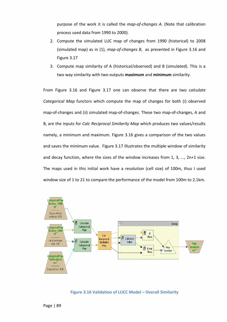
Page | 89

purpose of the work it is called the map-of-changes A. (Note that calibration

process used data from 1990 to 2000).

2. Compute the simulated LUC map of changes from 1990 (historical) to 2008

(simulated map) as in (1), map-of-changes B, as presented in Figure 3.16 and

Figure 3.17

3. Compute map similarity of A (historical/observed) and B (simulated). This is a

two way similarity with two outputs maximum and minimum similarity.

From Figure 3.16 and Figure 3.17 one can observe that there are two calculate

Categorical Map functors which compute the map of changes for both (i) observed

map-of-changes and (ii) simulated map-of-changes. These two map-of-changes, A and

B, are the inputs for Calc Reciprocal Similarity Map which produces two values/results

namely, a minimum and maximum. Figure 3.16 gives a comparison of the two values

and saves the minimum value. Figure 3.17 illustrates the multiple window of similarity

and decay function, where the sizes of the window increases from 1, 3, ..., 2n+1 size.

The maps used in this initial work have a resolution (cell size) of 100m, thus I used

window size of 1 to 21 to compare the performance of the model from 100m to 2.1km.

Figure 3.16 Validation of LUCC Model – Overall Similarity

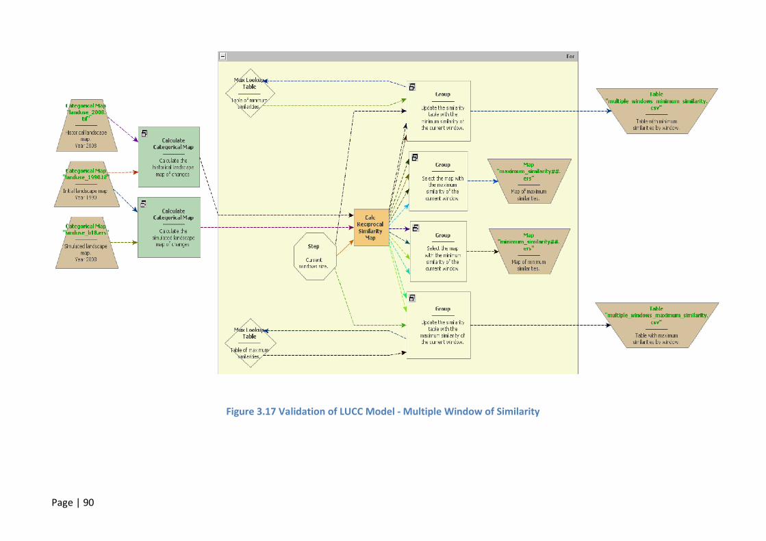
Page | 90

Figure 3.17 Validation of LUCC Model - Multiple Window of Similarity

Page | 91

Figure 3.18 Reciprocal Similarity Functor

Figure 3.19 Reciprocal Similarity - Fuzzy comparison method (Source :Soares-Filho et

al., 2009, p.75)

Page | 92

An example of reciprocal similarity computation is given in Figure 3.19, showing the

two way fuzzy applications. Details of the fuzzy, kappa and kfuzzy statistics are

discussed in detail in Visser(2004) and Hagen(2003).

In Figure 3.1, it can be seen that in the developed workflow process model if the

validation of the initial model (with WoE method of calibration) is not satisfactory then

the Genetic Algorithm is used to enhance the WoE of Coefficients of Variables.

In summary the working processes for modelling LUCC in DINAMICA EGO have been

explained including the underlying formulae. The WoE method was used for initial

calibration (fitness of parameter sets) and a fuzzy multiple-window-similarity approach

used in the validating the process. The Genetic Algorithm (GA) method can be used to

enhance the coefficients of parameters if the validation results of the initial calibration

are not acceptable. This GA method section of the process workflow model is

explained in the next chapter.

Page | 93

Chapter 4 Calibration of LUCC - GA Approach

Cellular Automata LUCC models employ transition rules and parameters to model

change from time t1 to t2. In the real world these transition rules and parameters are

not known but in LUCC models modellers have to choose or compute transition rules

for specific land use change classes of interest “ignoring” the rest. In order to ascertain

that the chosen transition’s rules and parameters are acceptable, a comparison of the

simulated maps with the observed (reference) maps is carried out in order to measure

the goodness-of-fit of the parameter set (Visser, 2004, p.85). For example, in

calibrating the LUCC model for Auckland from 1990 to 2000 (see section 7.6.1), the

observed (reference) land use cover change from 1990 - 2000 is compared with the

simulated land use cover change 1990 – 2000 and the result quantified. This result

informs the modeller of the level of uncertainty (goodness-of-fit) of the transition rules

and parameter sets used. Thus the LUCC model calibration process is aimed at finding

the optimal or most realistic transition rules and suitable parameter sets so that the

modelled change matches the actual observed change. The work reported in 0

resulted in the finding that this calibration process is sensitive to transition rules and

WoE of Coefficients variables. Therefore the calibration of the LUCC process aims to

find the optimal combination of transition rules and WoEs in a way that the modelled

change can match the real change. Thus the calibration process (to determine realistic

transition rules and parameter sets) is critical in validating (predictive power) the

model and is a challenge in LUCC modelling (Visser, 2004). One of the challenges in

choosing a suitable calibration method for cellular automata LUCC is the large

tessellated search area and the exponential rise in effort which occurs as the number

Page | 94

of variables increases and wider variable ranges are required for the transition rules.

For example, in the SLEUTH model, which employs a Monte Carlo approach to

calibration, the time to run the model increases (can take days to complete) as the

variable ranges increase (Clarke, 2012). Among the class of hard predictors, the

Genetic Algorithm(GA) method had been found to be a powerful means for calibrating

land use models (Eastman, Van Fossen, & Solorzano, 2005). GA uses a large amount of

computer resources and employs heuristics to search for the global optimum solution

for a set of model parameters by replicating the principle of biological evolution (Koza,

1998, p.430).

In light of the reported success in using GA’s to calibrate land use models it was

considered appropriate to use a GA approach to help improve the WoE coefficients of

parameters calibration method.

One of the known issues with GA is the potential to overspecialise the parameters of a

model. If overspecialisation occurs the forecasting (future scenario) accuracy is

affected. Thus it is important to validate the generated GA parameters over different

time periods to avoid over specialisation. This research will adopt a comparative

analysis of the calibration and validation results of both the WoE and the GA methods

to verify whether or not there is any improvement in model accuracy using the GA

method.

4.1 Definitions

The terminologies used in this thesis to explain the GA methodology are defined in this

section.

Page | 95

Individual: An individual refers to a set of WoE coefficients of parameters, for example

the set of WoE coefficients for distance-to-roads, distance-to-rivers, soil, and elevation

and other variables of LUCC model.

Population: Population is a set of individuals. The GA process sets an initial population

and population size at the start of iteration. The population (content) is randomly

generated for every iteration but size remains constant throughout.

Generation: The population generated for each iteration is a generation, thus the

number of generations determines the number of iterations in the GA process. If

convergence limit is not set then the number of iteration is used as the stopping

criteria.

Fitness: Is the result given by map comparison fuzzy similarity in order to evaluate the

fitness or appropriateness of an individual to continue on into the next generation.

4.2 GA Working Process for LUCC

Figure 4.2 represents the design of the GA calibration for LUCC and Figure 4.1 shows

the working process of the GA method. The set of WoEs coefficients of the LUCC

model variables are assembled into tables which serve as genomes/chromosomes

input for the GA process (Figure 4.2).

The population size and number of generations are initially configured before the

commencement of the GA process (Figure 4.1), thus the inputs for the GA process are:

Genes (WoE coefficients of variables)

Population size

Page | 96

Setting stopping criteria (either number of generation or convergence limit)

LUCC reference map

Figure 4.1 Workflow of GA Process

Page | 97

Figure 4.2 Design of GA LUCC Calibration Process

Page | 98

The DINAMICA EGO uses two different modes of termination as the fitness value

becomes asymptotic it either (a) iterates until number of iterations is equal to the

number of generations set by the user and/ or (b) iterates until convergence is

achieved. Whichever condition is met first terminates the execution of the

optimisation process.

During the GA process execution, the initial population of individuals (Population Size)

using the initial individual as a seed ("Individual Genotype") is generated and lower

and upper bounds of genes are set. These boundaries (lower and upper) constrain the

search for new genes within the boundary, thus optimising process time and providing

a trend for the finding the global optimum solution.

A seed (set of parameters) is used in running the model and its fitness value computed

using map comparison of fuzzy similarity approach. For every generation each of the

individuals of the population is used to run the model independently and its fitness

determined, then the fitness of all the individuals are compared and the individual

with the best fitness is saved internally for that generation. A meta heuristic

estimation method is used as the fitness function (k-Nearest Neighbour(KNN)

algorithm, Using KNN enables the model to compute fitness for a percentage of the

individuals and saves computer time and resources (Bremner et al., 2005; Soares-Filho

et al., 2009).

For the next generation a percentage of individuals from the current generation are

selected for reproduction using a Tournament Selection method (Miller & Goldberg,

1995). The GA process continues iteratively until the termination condition is met. The

Page | 99

fittest individual from the all the generations is returned as the optimal solution (see

Figure 4.1 and Figure 7.66).

The best individual parameter set as determined by the GA process will then be

validated and its result compared with those of WoE coefficient parameters (without

GA). If the validation results of GA parameter set is better than without GA then it

could be concluded that GA has helped in improving the calibration of the LUCC model

and as a consequence has improved the accuracy of the LUCC work flow process

model.

Figure 7.65 gives an example of the calibration of LUCC model using GA tool in

DINAMICA EGO whilst Figure 7.66 shows the details of the GA tool modelling.

This chapter has explained the process of Genetic Algorithm Calibration. This process

seeks to enhance on prime WoE coefficients of the parameter set by generating new

set of coefficients. Section 7.6 describes the implementation and evaluation of this

proposed GA-WoE approach to model calibration.

Page | 100

Chapter 5 Study Areas

In order to test the generic nature of the model and its performance, two different

geographic locations were chosen the Rondônia State of Brazil and the Auckland

Region of New Zealand as well as a specialised extension of the Auckland LUCC model

in order to model carbon sequestration.

In the Auckland Region though there are LUCCs, the rate of change is slow relative to

most largely urban regions (example Rondônia State). As a consequence the Auckland

region was a good choice for testing whether or not the proposed workflow modelling

process is sensitive to slow changes. The deforestation area of Rondônia State was

selected as a case study because of the rapid LUCC as a result of the deforestation of

the Amazon forest; this case study provides a means of testing the performance of the

model in a region subject to rapid changes.

These case studies were also used to evaluate the sensitivity of the proposed workflow

modelling process to the number of LUC classes. The LUC map for the Auckland region

consisted of seven classes with 42 possible transitions (a relatively complex LUCC

model) in contrast the Rondônia forest region had three classes and six possible

transitions (a simple LUCC model). The carbon sequestration is an extension of the

Auckland LUCC model which will be developed using the novel LUCC modelling

framework developed as part of this research (See Chapters 3 and 4). The Carbon

sequestration case study was included in order to demonstrate that the models

developed using the generic LUCC modelling framework can be used as a base models

for further study. The carbon sequestration case study LUCC model itself will also be

Page | 101

developed using the generic LUCC modelling framework, where the Auckland base

maps themselves generated by the LUCC modelling framework are used as input along

with LUC inputs related to Carbon Sequestration. These LUC inputs include vegetative

coverages such as such as natural forest, planted forest and grassland.

5.1 Auckland Region - Description

Auckland is the fastest growing metropolis in New Zealand and an inventory conducted

by Demorgraphia (2012) ranked Auckland among the world’s largest urban areas. The

“Quality of Living Survey Worldwide” conducted by Mercer (2012) ranked Auckland

city 3rd whilst The Economist’s Liveability Ranking and Overview (Economist Intelligent

Unit, 2012) in August placed Auckland in the 9th place. These are indications that

Auckland is an attractive city which is growing rapidly, thus the need to study its

growth dynamics that will enable decision makers to develop strategies to mitigate its

impact.

The Auckland Region is one of 16 regions and is located in the North Island as shown in

Figure 5.1. It is located between latitudes 36⁰ 09′ 00″South and 37⁰ 35′ 50″South, and

longitudes 174⁰ 09′ 00″East and 175⁰ 34′ 00″East. It encompasses the Auckland

Metropolitan area, rural towns, large areas of farmlands and vegetation, and the

Hauraki Gulf and Waiheke islands (Figure 5.1). It is by far the most populous region in

New Zealand with about 32.4% of country’s population and one of the smallest regions

(5,600km2 which is about 2% of 268,700 km2 of the total area of New Zealand).

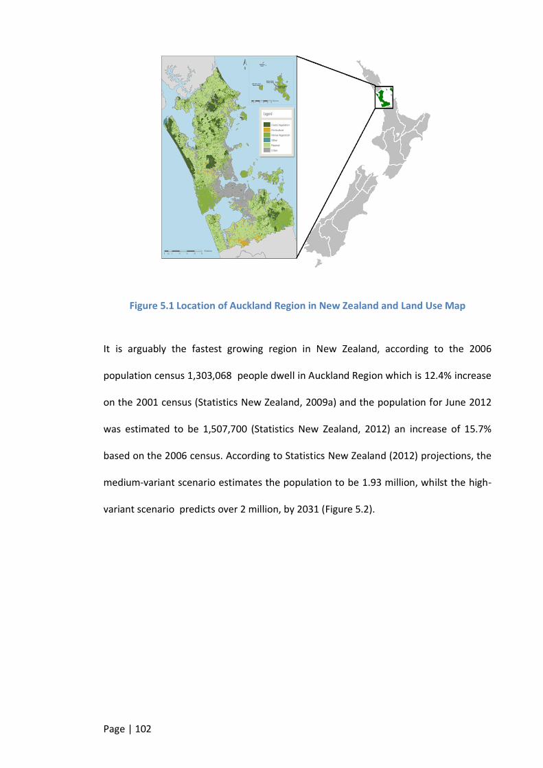
Page | 102

Figure 5.1 Location of Auckland Region in New Zealand and Land Use Map

It is arguably the fastest growing region in New Zealand, according to the 2006

population census 1,303,068 people dwell in Auckland Region which is 12.4% increase

on the 2001 census (Statistics New Zealand, 2009a) and the population for June 2012

was estimated to be 1,507,700 (Statistics New Zealand, 2012) an increase of 15.7%

based on the 2006 census. According to Statistics New Zealand (2012) projections, the

medium-variant scenario estimates the population to be 1.93 million, whilst the high-

variant scenario predicts over 2 million, by 2031 (Figure 5.2).

Page | 103

Figure 5.2 Population of Auckland Region : 1991 -2006 Cemsus, 2011 -2031

Projections (Source : Statistics New Zealand, 2009a)

Figure 5.3 shows the increase in population density for the Auckland region from 1991

to the projected density for 2013. The most notable increase over time in population

density is observed in the existing urban areas. The population dynamics of the region

is or will have a significant impact on LUC, especially urban sprawl, transportation

network and other infrastructure, thus it is necessary to address this proactively in

planning policy.

Over the years, measures to limit the regional growth and check urban sprawl has

been unsuccessful as the region has its unique dynamics in addition to population

growth (Statistics New Zealand, 1999). In addressing the future growth this research

work can help policy makers understand the driving factors of both historic and future

growth.

Page | 104

Figure 5.3 Population Density (persons per km2) Auckland Region. Census 1991-2006,

projection 2011 -2031. (Source : Statistics New Zealand,2009a)

5.1.1 The Land and Environment

The nature of land and its environs can contribute to the changes that occur on the

landscape. For example urban growth is usually found in low lying areas whilst steep

slopes do not encourage settlements, also the type of soil and climate could determine

which vegetation or crops can grow in the area. A good knowledge of the land and

environment helps in determining or “selecting” some of the driving factors for the

model.

Page | 105

Topography: The length of the region stretching from north to south is approximately

120km and its breadth measures 60km from the west to east. The region has a long

stretch of coastal land on both the east and west so there are several harbours and

bays. The northern boundary is defined by the Kaipara Harbour inlet and the southern

boundary is marked by the Bombay and Pukekohe Hills. On the western side lies the

Waitakere Ranges which is favourable for native forests consisting of subtropical and

temperate rainforests species. On the eastern side is the Hauraki Gulf made up of

many islands. The landscape of the region is punctuated with more than 50 volcanic

cones, lakes, lagoons islands and depressions with the oldest volcano over 150,000

years and the most recent volcano (Rangitoto) is approximately 700 years old and its

last eruption according local Māori iwi was 600 years ago (Smith & Allen, 2010).

Climate: Auckland climate is characterised as warm-temperate with mild, damp

winters and warm, humid summers. According to the National Institute of Water and

Atmospheric Research (NIWA New Zealand, 2012), frequent and high levels of rainfall

are recorded in Auckland Region throughout the year with an average of 1240mm per

annum. Snowfall in Auckland is very rare but recorded an instance was recently on 15th

August 2011 in the suburb of Henderson Heights. In mid-summer Auckland records an

average daily maximum temperature of around 23⁰C and in mid-winter a minimum of

8⁰C.

Soil: The soil composition of an area determines the way in which the land is likely to

be used. For example a land rich in loamy soil might be suitable for growing crops,

rocky (granite) land could be used as a quarry whilst sedimentary rocks might be good

for mining minerals or oil. Consequently, the type of soil is a potential predictive

variable in LUCC. The soil of the Auckland Region is generally lime deficient and the

Page | 106

western and southern zones are potassium deficient. However, deposits of lava from

volcanic activity has resulted in distribution of rich fertile loams (an even composition

of sand, silt and clay and decay of organic matter) resulting in soil with a high nutrient

content(Statistics New Zealand, 1999).

Environment: The discussion in 2.3.1 illustrated that human interaction with land and

its environments results in changes in land use and cover therefore population growth

is of concern for many towns and regional councils because of its potential impact on

the environment. In the Auckland region, this concern is elevated due to the rapid

population growth over the recent years. This unprecedented growth has placed

significant pressure on the existing transportation network, sewage treatment and

refuse disposal infrastructure. Expansion of these infrastructures may result in a

significant increase in the level of air, water and soil pollution if measures are not put

in place to ensure that the expansion is planned to minimised the environmental

impact. These effects on the environment especially land could result in major changes

in the landscape. For example if expansion of transportation network comprises of

widening and increasing roads, rather than public transport, it is likely that many more

cars will use the road resulting in an increase in release of CO2 into the atmosphere.

This may negatively affect the environment of the region. Polluted soil and/or water

may affect crop growth which in turn affects the viability of the land for growing crops

resulting in a change of land usage in the region.

Land Use/Cover: The New Zealand Ministry for the Environment (MfE) has developed

spatial Land Use Map (LUM) data for the entire country. This data is generally

accepted by land use professionals as the standard reference map from New Zealand

(Ministry for Environment, 2011). This data is composed of 12 land use classifications

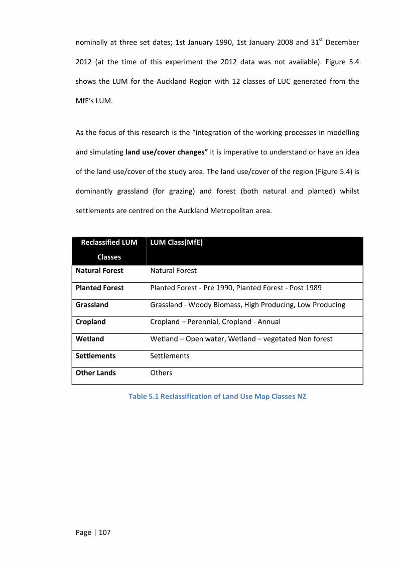
Page | 107

nominally at three set dates; 1st January 1990, 1st January 2008 and 31st December

2012 (at the time of this experiment the 2012 data was not available). Figure 5.4

shows the LUM for the Auckland Region with 12 classes of LUC generated from the

MfE’s LUM.

As the focus of this research is the “integration of the working processes in modelling

and simulating land use/cover changes” it is imperative to understand or have an idea

of the land use/cover of the study area. The land use/cover of the region (Figure 5.4) is

dominantly grassland (for grazing) and forest (both natural and planted) whilst

settlements are centred on the Auckland Metropolitan area.

Reclassified LUM

Classes

LUM Class(MfE)

Natural Forest Natural Forest

Planted Forest Planted Forest - Pre 1990, Planted Forest - Post 1989

Grassland Grassland - Woody Biomass, High Producing, Low Producing

Cropland Cropland – Perennial, Cropland - Annual

Wetland Wetland – Open water, Wetland – vegetated Non forest

Settlements Settlements

Other Lands Others

Table 5.1 Reclassification of Land Use Map Classes NZ

Page | 108

Figure 5.4 Land Use Map of Auckland Region

5.1.2 Why Auckland Region?

In recent past the human activities in Auckland Region have increased significantly and

the council is faced with managing the growth and having in place policies and plans

for future growth. In view of this many researchers have studied the growth and

shared their thoughts on how to manage the growth and mitigate future scenarios.

Most of these researches focused on the expansion of housing units, transportation

network and managing urban land. There is no published research in the area of land

use/cover change simulation models for the Auckland Region and no work has been

reported that investigates the drivers of land use/cover change with the aim of

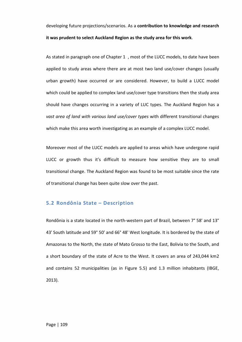
Page | 109

developing future projections/scenarios. As a contribution to knowledge and research

it was prudent to select Auckland Region as the study area for this work.

As stated in paragraph one of Chapter 1 , most of the LUCC models, to date have been

applied to study areas where there are at most two land use/cover changes (usually

urban growth) have occurred or are considered. However, to build a LUCC model

which could be applied to complex land use/cover type transitions then the study area

should have changes occurring in a variety of LUC types. The Auckland Region has a

vast area of land with various land use/cover types with different transitional changes

which make this area worth investigating as an example of a complex LUCC model.

Moreover most of the LUCC models are applied to areas which have undergone rapid

LUCC or growth thus it’s difficult to measure how sensitive they are to small

transitional change. The Auckland Region was found to be most suitable since the rate

of transitional change has been quite slow over the past.

5.2 Rondônia State – Description

Rondônia is a state located in the north-western part of Brazil, between 7° 58' and 13°

43' South latitude and 59° 50' and 66° 48' West longitude. It is bordered by the state of

Amazonas to the North, the state of Mato Grosso to the East, Bolivia to the South, and

a short boundary of the state of Acre to the West. It covers an area of 243,044 km2

and contains 52 municipalities (as in Figure 5.5) and 1.3 million inhabitants (IBGE,

2013).

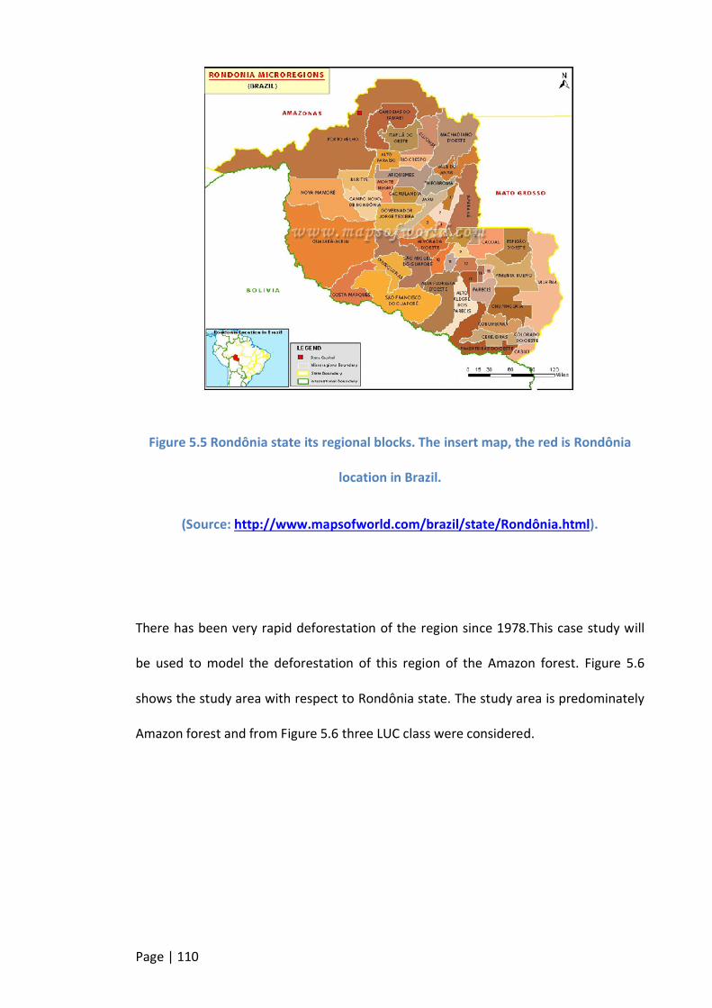
Page | 110

Figure 5.5 Rondônia state its regional blocks. The insert map, the red is Rondônia

location in Brazil.

(Source: http://www.mapsofworld.com/brazil/state/Rondônia.html).

There has been very rapid deforestation of the region since 1978.This case study will

be used to model the deforestation of this region of the Amazon forest. Figure 5.6

shows the study area with respect to Rondônia state. The study area is predominately

Amazon forest and from Figure 5.6 three LUC class were considered.

Page | 111

Figure 5.6 Study area with respect to Rondônia state and Brazil

5.2.1 The Land and Environments

Climate: The state's climate is predominantly equatorial, with a tropical transition. It is

hot and humid throughout the year, with a large yearly temperature range. The daily

temperature ranges are also notable, especially during the winter. Throughout the

summer, convective activity, caused by a greater incidence of solar radiation, is high.

The winter season is characterized by fluvial winds and increased rains influenced by

ecosystems in the Inter-tropical Convergence Zone and the Bolivian Highlands. The

rainiest period in the region is between November and March (winter). The driest

period (with less convective activity) is between May and September (summer). The

region's annual rainfall is approximately 1800. (www.rondomia.ro.gov.br)

Landform: The region contains five main geomorphological environments which

include areas of regional surface levelling domain divided into levels I, II and III;

Page | 112

mountain chains composed of old sedimentary rock in the form of tabular surfaces;

areas of tertiary sedimentary rock; slopes and hills associated with the presence of

erosion resistant rock that highlight the regional levelling surface and the Madeira

river system, including the Mamoré, Guaporé, Ji-Paraná and Roosevelt subsystems.

Soil: The soils in Rondônia are predominantly Argisols, Combisols, Gleisols, Latosols

and Neosols. Approximately half of the state land is Latosols; of which 26% are Red-

Yellow Latosols and 16% are Red-Yellow and Red Latosols. Most of the amazon tropical

rain forest is on Latosols soil. It has rich fertile top layer due to falling leaves and

branches from the rain forest. Deforestation is the major cause of leaching of nutrients

leaving high mercury concentrations in the latosols which does not support farming(M.

Almeida, Lacerda, Bastos, & Herrmann, 2005).

Land Use Cover: The state which 30 years ago consisted of about 208,000 square

kilometres of rain forest has become one of the most deforested parts of the Amazon

forest. There has been rapid clearing and degradation of the natural forest in the past

three decades: about 4,200 square kilometres had been cleared by 1978; 30,000 by

1988; and 53,300 by 1998. An estimated 67,764 square kilometres was cleared by

2003. The LUC map of the study area, shown in Figure 5.7, is classified into three

classes namely; forest land, deforested land and non-vegetation. The flora of the

region is made up of a large biodiversity of species because the region is in a transition

area between the Cerrado, Pantanal, and Amazon regions (NASA, 2013).

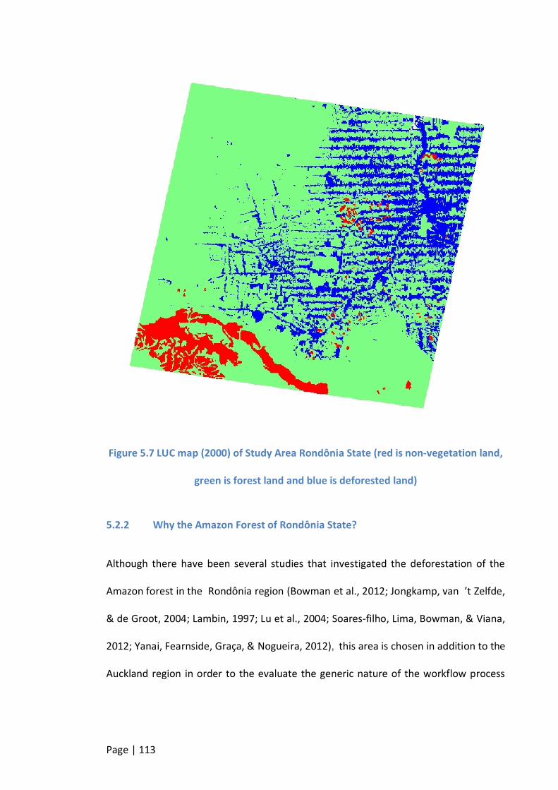
Page | 113

Figure 5.7 LUC map (2000) of Study Area Rondônia State (red is non-vegetation land,

green is forest land and blue is deforested land)

5.2.2 Why the Amazon Forest of Rondônia State?

Although there have been several studies that investigated the deforestation of the

Amazon forest in the Rondônia region (Bowman et al., 2012; Jongkamp, van ’t Zelfde,

& de Groot, 2004; Lambin, 1997; Lu et al., 2004; Soares-filho, Lima, Bowman, & Viana,

2012; Yanai, Fearnside, Graça, & Nogueira, 2012), this area is chosen in addition to the

Auckland region in order to the evaluate the generic nature of the workflow process

Page | 114

model. This case study is less complex with fewer transitions to consider than for the

Auckland study.

5.3 Vegetation Carbon Sequestration

The Kyoto protocol, an international agreement concluded in 1997 addressed global

warming and introduced measures to reduce the rate of climate change. Its main aim

was to reduce the human emitted greenhouse gases of developing and developed

countries to 5% below their 1990 emission baseline (Grubb, 2004). One of the

anthropogenic greenhouse gases is carbon dioxide (CO2) and the removal of carbon

from the atmosphere is known as carbon sequestration or carbon sink. In the context

of this thesis carbon sequestration refers to the natural biochemical cycling of carbon

between the atmosphere and vegetation. Vegetative carbon sequestration is the

process by which carbon dioxide is absorbed by plants during photosynthesis and is

stored in their leaves, branches, trunks and roots. One possible way of mitigating or at

least slowing the amount of human carbon emissions is via afforestation or

reforestation of land in order to incorporate carbon from atmospheric CO2 into

biomass. Of course this approach is only successful if the carbon is not then returned

to the atmosphere as a result of burning or rotting when the trees die. To prevent the

return of carbon trees must grow in perpetuity (with no deforestation) or the carbon

from them must itself be sequestered by some other means.

In this research the Vegetative Carbon Sequestration Scenario will be used to project

annual carbon sequestration, for the Auckland region, based on historic trends in

natural forest, planted forest and grassland LUC changes. Forest Carbon stock

computation is contentious because of differences in absorption rates for different

Page | 115

species and types of vegetation., In view of the differences between species flat rates

of carbon sequestration provided by Ministry of Primary Industries (2011) were used

for this case study.

5.3.1 Why Carbon Sequestration?

If the proposed framework is truly generic and performs well, then the generated

annual simulated LUC maps should provide a suitable base map for further studies.

Therefore the carbon sequestration scenario modelling is included in this research to

demonstrate that the LUCC model could be used as basis for advance study.

5.4 Summary

The two selected study areas are well suited for this work because the model can be

said to be generic if it performs well for different geographical locations with differing

numbers of model parameters and different spatial resolutions. Because of the

different number of LUCC transitions in the two areas, one for Rondônia and seven for

Auckland; it is also possible to test the performance of the model with scenarios of

different complexities.

Page | 116

Chapter 6 Land Use/Cover Change Model Data

This chapter gives an overview of the data used in modelling the LUCC for the Auckland

Region, Rondônia Amazon forest, and Carbon sequestration. It details their sources,

acquisition and preparation.

Spatial datasets form the foundation for LUCC modelling and the choice of spatial data

structure is dependent on the modelling method. In GIS there are two basic spatial

data models vector and raster. The Spatial Vector Data Model represents geographic

objects as points, lines and polygons with associated tabular attribute data. The

geographic object used typically reflects the dimension of the attribute, for example

cities and towns are represented as points; rivers, roads and elevation as lines; areas of

land use/cover as polygons. The Raster Spatial Data Model uses a grid of cells (pixels)

to represent geographic data. A raster cell is often also referred to as a pixel (picture

element). A raster data pixel stores data values within a specified range or colour

depth. These values may represent a value within a colour scale or within a grey scale,

as well as depth or height, or any other thematic value, such as a land use/cover class

index (Longley et al., 2010, p. 87-88). Two categories of raster data used are:

Thematic/Categorical – land use/cover and soil data

Continuous – slope, elevation and distance maps

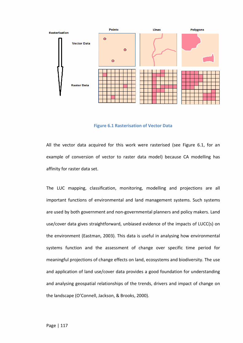
Page | 117

Figure 6.1 Rasterisation of Vector Data

All the vector data acquired for this work were rasterised (see Figure 6.1, for an

example of conversion of vector to raster data model) because CA modelling has

affinity for raster data set.

The LUC mapping, classification, monitoring, modelling and projections are all

important functions of environmental and land management systems. Such systems

are used by both government and non-governmental planners and policy makers. Land

use/cover data gives straightforward, unbiased evidence of the impacts of LUCC(s) on

the environment (Eastman, 2003). This data is useful in analysing how environmental

systems function and the assessment of change over specific time period for

meaningful projections of change effects on land, ecosystems and biodiversity. The use

and application of land use/cover data provides a good foundation for understanding

and analysing geospatial relationships of the trends, drivers and impact of change on

the landscape (O’Connell, Jackson, & Brooks, 2000).

Page | 118

6.1 Data Description

The monitoring and modelling of land use/cover change requires empirical spatial data

spanning a period of time. For this research the land use/cover data for Auckland for

the years 1990, 2000 and 2008 was used. LUC Data for 1990 and 2000 was used for

calibration of the model whilst for validation of the model, 1990 and 2008 data was

used; this is illustrated in Figure 6.2. For Rondônia LUC maps for 1997, 2000 and 2003

were used and the data from 1997 to 2000 was used for calibration. Data covering the

period of 1997 to 2003 was used to validate the Rondônia deforestation LUCC model.

For the LUC model to make reliable projections it was imperative to validate it with

LUC data beyond (ahead) the time frame of the calibration thus the use of 2008 LUC

data, for Auckland and 2003 for Rondônia.

Figure 6.2 Illustration of LUC Data and Time Frame

In addition to LUC data, ancillary data digital elevation model (DEM), slope, major and

minor roads, rivers, soil, population and reserved lands were considered as drivers of

LUCC

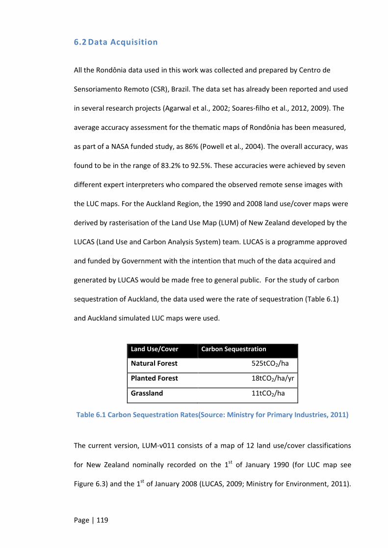
Page | 119

6.2 Data Acquisition

All the Rondônia data used in this work was collected and prepared by Centro de

Sensoriamento Remoto (CSR), Brazil. The data set has already been reported and used

in several research projects (Agarwal et al., 2002; Soares-filho et al., 2012, 2009). The

average accuracy assessment for the thematic maps of Rondônia has been measured,

as part of a NASA funded study, as 86% (Powell et al., 2004). The overall accuracy, was

found to be in the range of 83.2% to 92.5%. These accuracies were achieved by seven

different expert interpreters who compared the observed remote sense images with

the LUC maps. For the Auckland Region, the 1990 and 2008 land use/cover maps were

derived by rasterisation of the Land Use Map (LUM) of New Zealand developed by the

LUCAS (Land Use and Carbon Analysis System) team. LUCAS is a programme approved

and funded by Government with the intention that much of the data acquired and

generated by LUCAS would be made free to general public. For the study of carbon

sequestration of Auckland, the data used were the rate of sequestration (Table 6.1)

and Auckland simulated LUC maps were used.

Land Use/Cover Carbon Sequestration

Natural Forest 525tCO2/ha

Planted Forest 18tCO2/ha/yr

Grassland 11tCO2/ha

Table 6.1 Carbon Sequestration Rates(Source: Ministry for Primary Industries, 2011)

The current version, LUM-v011 consists of a map of 12 land use/cover classifications

for New Zealand nominally recorded on the 1st of January 1990 (for LUC map see

Figure 6.3) and the 1st of January 2008 (LUCAS, 2009; Ministry for Environment, 2011).

Page | 120

The LUM version used in this work is LUM-v003 which was the latest at the time of

data preparation, covering 1990 and 2008.

A LUCAS developed LUM from a range of satellite imagery using the NZGD2000 datum

and the New Zealand Transverse Mercator Projection. LUCAS derived the 1990 LUM

dataset from 30m spatial resolution LandSat4 and LandSat5 satellite imagery from a

range of dates between 1988 and 1993. After orthorectification and atmospheric

correction, the satellite imagery was standardised for spectral reflectance using Ecosat

algorithms (Dymond & Shepherd, 2004). These standardised images were the used for

land use/cover classification. This classification process was validated and improved

using 15 m resolution Landsat 7 ETM+ imagery and SPOT 2 and 3 datasets coupled

with aerial photography (Ministry for Environment, 2011).

Page | 121

Figure 6.3 LUCAS land Use Map of New Zealand – 1990, red box indicates the

Auckland case study region.

The 2008 LUM was developed by LUCAS from 10m spatial resolution SPOT 5 satellite

imagery. The imagery was standardised for reflectance using the same algorithm as

was used for the 1990 imagery. The SPOT 5 imagery was taken during the summer

periods between November 2006 and April 2008, in order to establish a national set of

cloud-free imagery. Where the SPOT 5 imagery pre-dates the 1st of January 2008, a

combination of aerial photography, Moderate Resolution Imaging Spectroradiometer

Page | 122

(MODIS) satellite imagery and field verification was used to identify locations where

deforestation has occurred, so that the 2008 land-use map is as up-to-date as possible.

Since the 2000 LUC map was not included in the LUM-003 data, this work generated it

using 15m LandSat7 ETM+ imagery for 2000-2001 coupled with aerial photography.

For data consistency the same the same methodology used by LUCAS was used in

deriving the LUC map.

Figure 6.4 Digital Elevation Model (2m), Auckland Region

Page | 123

In addition to the LUC dataset ancillary data for the study areas such as; elevation,

slope, hillshade, soil, rivers, roads, and reserved lands. Thus ancillary data was

employed as the drivers for the LUCC model. A 2m Digital Elevation Model (DEM) was

obtained from the Auckland Regional Council. The Regional Council derived the DEM

image, in Figure 6.4, from LiDAR (Light Detection And Ranging) imagery. The Regional

Council provided a dataset for the protected/reserved lands and parks of Auckland.

Figure 6.5 Hillshade, Auckland Region

Page | 124

As part of the data pre-processing for this research work the slope (Figure 6.6) and

hillshade (Figure 6.5) datasets were extracted from the supplied DEM using ArcGIS

Spatial Analyst tool, . The road and river network data of Auckland region were

obtained from the Land Information New Zealand’s website, www.data.linz.govt.nz ,

which is a repository of government funded land information datasets for New

Zealand.

Figure 6.6 Slope, Auckland Region

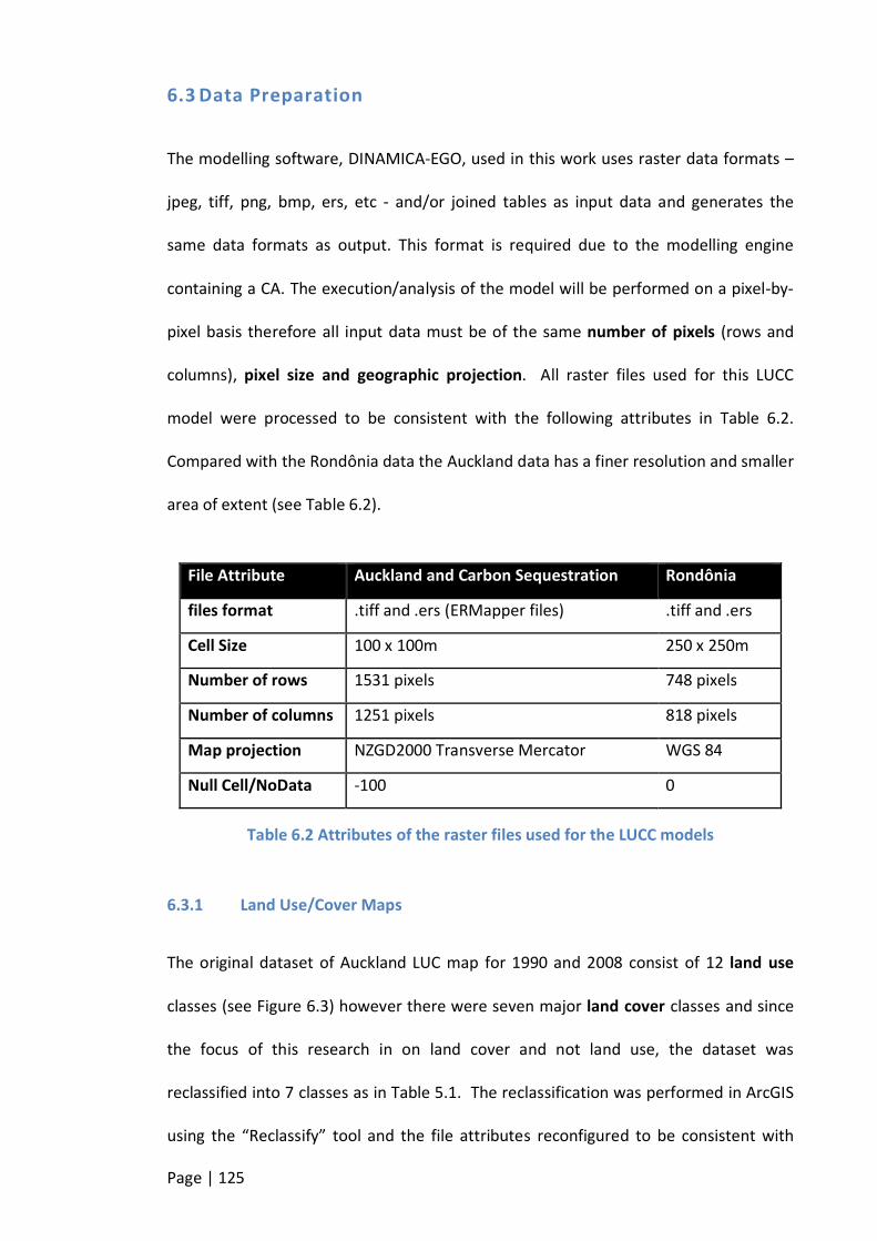
Page | 125

6.3 Data Preparation

The modelling software, DINAMICA-EGO, used in this work uses raster data formats –

jpeg, tiff, png, bmp, ers, etc - and/or joined tables as input data and generates the

same data formats as output. This format is required due to the modelling engine

containing a CA. The execution/analysis of the model will be performed on a pixel-by-

pixel basis therefore all input data must be of the same number of pixels (rows and

columns), pixel size and geographic projection. All raster files used for this LUCC

model were processed to be consistent with the following attributes in Table 6.2.

Compared with the Rondônia data the Auckland data has a finer resolution and smaller

area of extent (see Table 6.2).

File Attribute Auckland and Carbon Sequestration Rondônia

files format .tiff and .ers (ERMapper files) .tiff and .ers

Cell Size 100 x 100m 250 x 250m

Number of rows 1531 pixels 748 pixels

Number of columns 1251 pixels 818 pixels

Map projection NZGD2000 Transverse Mercator WGS 84

Null Cell/NoData -100 0

Table 6.2 Attributes of the raster files used for the LUCC models

6.3.1 Land Use/Cover Maps

The original dataset of Auckland LUC map for 1990 and 2008 consist of 12 land use

classes (see Figure 6.3) however there were seven major land cover classes and since

the focus of this research in on land cover and not land use, the dataset was

reclassified into 7 classes as in Table 5.1. The reclassification was performed in ArcGIS

using the “Reclassify” tool and the file attributes reconfigured to be consistent with

Page | 126

Table 6.2. The LUC map for the year 2000 was developed using GIS and RS with using

“ENVI EX” (for RS designed to enable feature extraction and classification) and ArcGIS

software.

Table 6.3 is a quantitative representation of the Auckland LUC classes for 1990 and

2000 which shows the total area in pixels of the class for each year. For example in row

one of Table 6.3 it can be seen that Natural Forest (LUC Class 1) covered an area of

145, 587 pixels in 1990 and 145,207 pixels in 2000 indicating that there was a loss of

380 pixels to other LUCs over this ten year period. Table 6.4 provides similar details for

the Rondônia forest area.

Table 6.3 provides a comparison of the total number of pixels for each Auckland LUC

class for the years 1990 and 2000 and Table 6.4 gives a summary of the number of

transitional pixels per LUC class from 1997 to 2000 for the Rondônia Forest area. The

difference between the cell counts is the “cell count latter year” minus “cell count

former year”, where positive values indicate growth in land use whilst negative values

indicate a reduction in land use for each class. An example is provided in Table 6.3

where the difference from 1990 to 2000 in Natural Forest (class 1) is -380 cells,

meaning that there was 380 hectares (one cell is 100x100m) loss of Natural Forest and

an increase of 6,112 hectares of Planted Forest. It is important to note from Table 6.3

that for Auckland there was no transitional change observed in Cropland and Wetland

and for Rondônia the non-vegetation land did not undergo any change between 1997

and 2000.

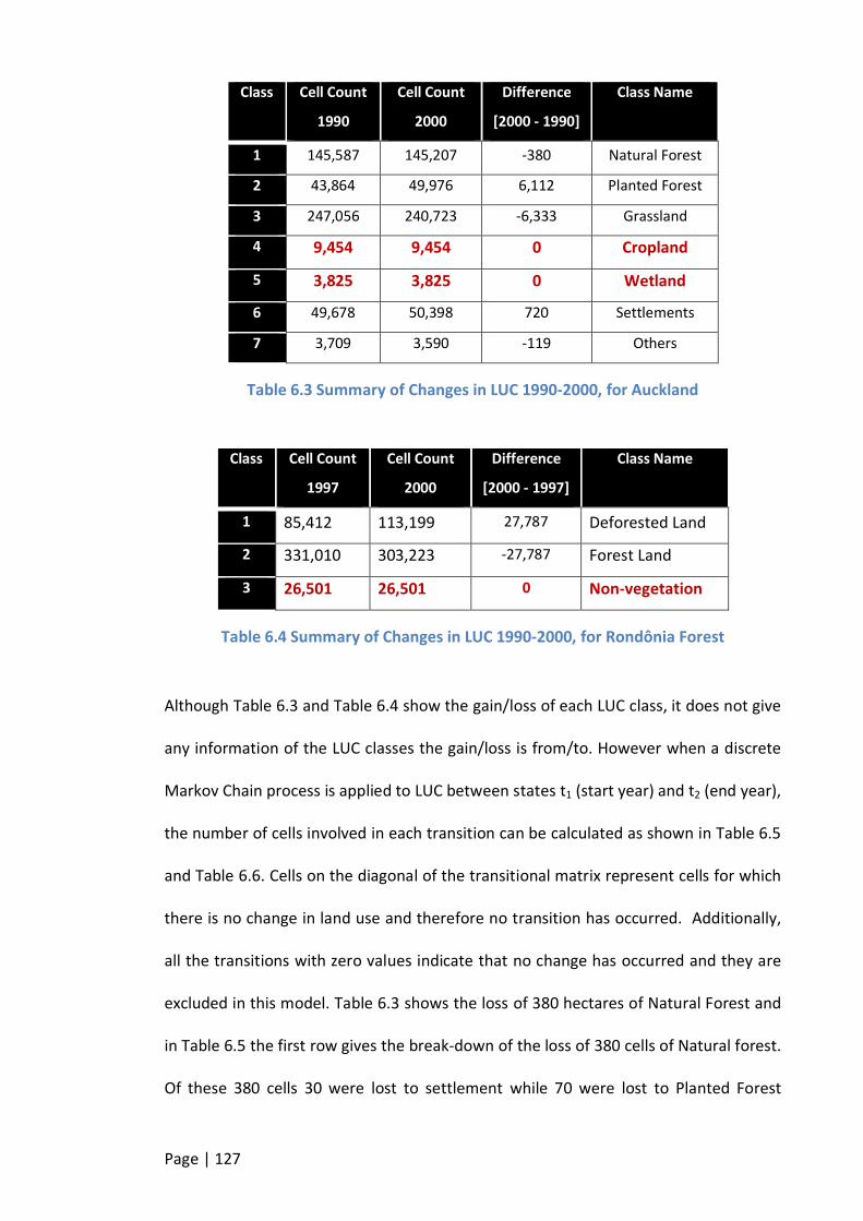
Page | 127

Class Cell Count

1990

Cell Count

2000

Difference

[2000 - 1990]

Class Name

1 145,587 145,207 -380 Natural Forest

2 43,864 49,976 6,112 Planted Forest

3 247,056 240,723 -6,333 Grassland

4 9,454 9,454 0 Cropland

5 3,825 3,825 0 Wetland

6 49,678 50,398 720 Settlements

7 3,709 3,590 -119 Others

Table 6.3 Summary of Changes in LUC 1990-2000, for Auckland

Class Cell Count

1997

Cell Count

2000

Difference

[2000 - 1997]

Class Name

1 85,412 113,199 27,787 Deforested Land

2 331,010 303,223 -27,787 Forest Land

3 26,501 26,501 0 Non-vegetation

Table 6.4 Summary of Changes in LUC 1990-2000, for Rondônia Forest

Although Table 6.3 and Table 6.4 show the gain/loss of each LUC class, it does not give

any information of the LUC classes the gain/loss is from/to. However when a discrete

Markov Chain process is applied to LUC between states t1 (start year) and t2 (end year),

the number of cells involved in each transition can be calculated as shown in Table 6.5

and Table 6.6. Cells on the diagonal of the transitional matrix represent cells for which

there is no change in land use and therefore no transition has occurred. Additionally,

all the transitions with zero values indicate that no change has occurred and they are

excluded in this model. Table 6.3 shows the loss of 380 hectares of Natural Forest and

in Table 6.5 the first row gives the break-down of the loss of 380 cells of Natural forest.

Of these 380 cells 30 were lost to settlement while 70 were lost to Planted Forest

Page | 128

(managed rather than native) and 280 cells to Grassland. Details of change and the

drivers of these LUC transitions are very important in modelling LUCC.

LUC

Map

fo

r t

1 =

19

90

LUC Map for t2 = 2000

1 2 3 4 5 6 7

1 xxxx 70 280 0 0 30 0

2 0 xxxx 60 0 0 0 0

3 0 6052 xxxx 0 0 640 10

4 0 0 0 xxxx 0 0 0

5 0 0 0 0 xxxx 0 0

6 0 0 0 0 0 xxxx 0

7 0 50 29 0 0 50 xxxx

Table 6.5 Auckland, Transitional Matrix

LUC Map 2000

1 2 3

LUC

Map

199

7 1 xxxx 0 0

2 27,787 xxxx 0

3 0 0 xxxx

Table 6.6 Rondônia, Transitional Matrix

As a result of the Markov Chain process, see Table 6.5, for the complex model only ten

LUC transitions have occurred. These transitions are the ones that were considered for

modelling the LUCC for the Auckland region, these key transitions are further detailed

in Table 6.7. Only one transitional change namely deforestation was discovered, using

the Markov Chain process, for Rondônia. This means that the Rondônia forest area is a

relatively simple, one transition LUCC model (Table 6.6).

To From

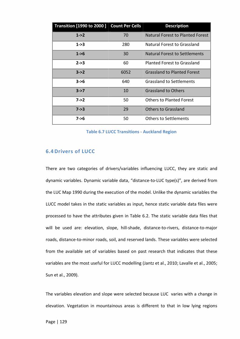
Page | 129

Transition [1990 to 2000 ] Count Per Cells Description

1->2 70 Natural Forest to Planted Forest

1->3 280 Natural Forest to Grassland

1->6 30 Natural Forest to Settlements

2->3 60 Planted Forest to Grassland

3->2 6052 Grassland to Planted Forest

3->6 640 Grassland to Settlements

3->7 10 Grassland to Others

7->2 50 Others to Planted Forest

7->3 29 Others to Grassland

7->6 50 Others to Settlements

Table 6.7 LUCC Transitions - Auckland Region

6.4 Drivers of LUCC

There are two categories of drivers/variables influencing LUCC, they are static and

dynamic variables. Dynamic variable data, “distance-to-LUC type(s)”, are derived from

the LUC Map 1990 during the execution of the model. Unlike the dynamic variables the

LUCC model takes in the static variables as input, hence static variable data files were

processed to have the attributes given in Table 6.2. The static variable data files that

will be used are: elevation, slope, hill-shade, distance-to-rivers, distance-to-major

roads, distance-to-minor roads, soil, and reserved lands. These variables were selected

from the available set of variables based on past research that indicates that these

variables are the most useful for LUCC modelling (Jantz et al., 2010; Lavalle et al., 2005;

Sun et al., 2009).

The variables elevation and slope were selected because LUC varies with a change in

elevation. Vegetation in mountainous areas is different to that in low lying regions

Page | 130

(Shrestha & Zinck, 2001; Xie, Sha, & Yu, 2008). There are many agricultural practices in

the catchment area of rivers and water bodies, also the banks of rivers naturally

support vegetation/forest. Therefore the distance-to-rivers was considered because of

its influence on the LUCC. The distance-to-roads variables were selected because the

accessibility and or proximity of roads to land influences human activities on the land

thus impacting on the land cover. The texture and fertility of soils determines the

vegetation that could be supported thus its inclusion. Crop growth is influenced by the

direction of the sun therefore the hillshade variable was also considered for the model.

The slope and hillshade data was derived from the elevation raster data. Distance-to-

major roads, distance-to-minor roads and distance-to-rivers were computed using the

map algebra method “compute distance maps” available in DINAMICA EGO. The

resultant distance map arises from a computation of the distances from a reference

point to each cell of a map. These distance maps help determine how the distance to

roads and rivers influences land use/cover change. Figure 6.7, Figure 6.8 and Figure

6.9 provide three distance maps for distance-to-major, distance-to-minor roads and

distance-to-rivers respectively.

Page | 131

Figure 6.7 Distance-to-Major Roads

Figure 6.8 Distance-to-Minor Roads

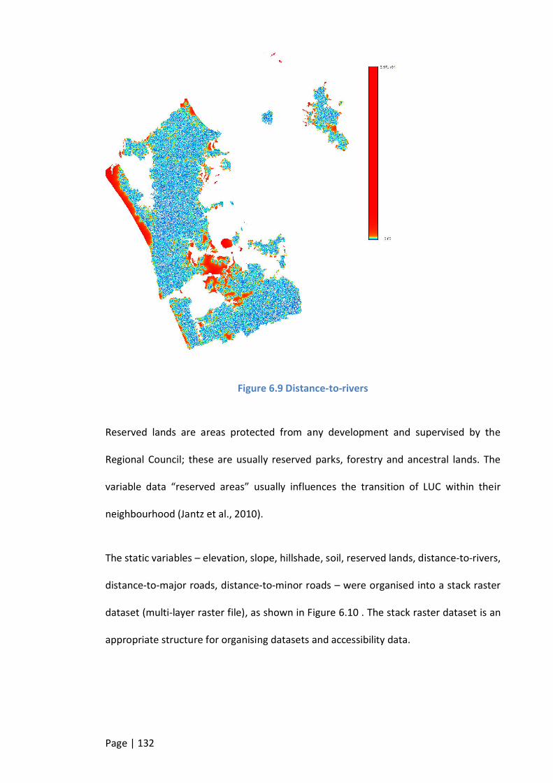
Page | 132

Figure 6.9 Distance-to-rivers

Reserved lands are areas protected from any development and supervised by the

Regional Council; these are usually reserved parks, forestry and ancestral lands. The

variable data “reserved areas” usually influences the transition of LUC within their

neighbourhood (Jantz et al., 2010).

The static variables – elevation, slope, hillshade, soil, reserved lands, distance-to-rivers,

distance-to-major roads, distance-to-minor roads – were organised into a stack raster

dataset (multi-layer raster file), as shown in Figure 6.10 . The stack raster dataset is an

appropriate structure for organising datasets and accessibility data.

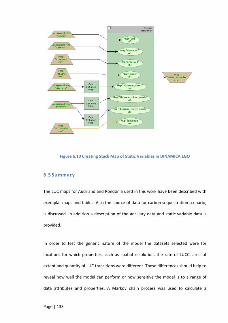
Page | 133

Figure 6.10 Creating Stack Map of Static Variables in DINAMICA EGO

6.5 Summary

The LUC maps for Auckland and Rondônia used in this work have been described with

exemplar maps and tables. Also the source of data for carbon sequestration scenario,

is discussed. In addition a description of the ancillary data and static variable data is

provided.

In order to test the generic nature of the model the datasets selected were for

locations for which properties, such as spatial resolution, the rate of LUCC, area of

extent and quantity of LUC transitions were different. These differences should help to

reveal how well the model can perform or how sensitive the model is to a range of

data attributes and properties. A Markov chain process was used to calculate a

Page | 134

transitional matrix to determine which LUC transitions occur for the Auckland and

Rondônia case study areas. And this approach confirmed that the Auckland LUCC is a

relatively complex model when compared with the deforestation of the Rondônia

Amazon forest. The variety in the level of complexity modelled will allow for the

performance of the model in both simple and complex simulation models to be

evaluated. Moreover the rate of deforestation in amazon forest of Rondônia is very

rapid when compared with the rate of LUC change in the Auckland region. As a result

these two study areas provide suitable cases to evaluate the generic nature of the

proposed LUCC model.

Page | 135

Chapter 7 Implementation and Results

The sensitivity of any set of variables to transitional change is the core task in

developing a spatio-temporal LUCC model. In light of this the performance of the

entire modelling processing depends mainly on the reliability of the set of variables per

transition. As mentioned earlier in the introductory chapter, the challenge for an LUCC

modeller is to adequately determine the set of variables for a specific location. Most

modellers use existing models with predefined variables that may or may not be

adequate for their purposed and adjust the coefficients for these predefined variables

during the calibration phase to adjust the influence of these variables. The proposed

workflow process model in 0 could help modellers determine the adequacy of the

variables used in a LUCC model. In order to evaluate this approach, the generic

workflow process model developed in this research was applied to Auckland and

Rondônia state forest and the Auckland case study was extended to model carbon

sequestration for the region.

This chapter presents the implementation of the workflow process explained in 0 and

an analysis of the results of applying this novel process to three case studies. The work

flow process model presented in Chapter 3 is a sequence of integrated working

processes (see Figure 3.1), in order to analyse and discuss all of the phases in the

workflow process, each phase is modelled separately. The integrated process is

analysed and discussed at the end of the chapter. The simulation platform adopted for

implementation is DINAMICA EGO (see Section 2.9 for a discussion of this).

The LUC maps used in the model have the following classes in Table 7.1 and Table 7.2.

Page | 136

Class/Key Class Name

1 Natural Forest

2 Planted Forest

3 Grassland

4 Cropland

5 Wetland

6 Settlements

7 Others

Table 7.1 Auckland LUC Classes and Names


1 Deforested land

2 Natural Forest

3 Non-vegetation

Table 7.2 Rondônia LUC Classes and Names

7.1 Computation of Transition Matrix of LUCC

What follows is a discussion of the calculation of the LUC transition matrices for the

Auckland and Rondônia case study areas. These matrices will be used to determine the

quantity of change from one LUC to another at the specified time unit.

7.1.1 Auckland Region

The “Determine Transition Matrix” operator in DINAMICA EGO was used to compute

historic LUC transition matrices for Auckland. The details of the formula underlying the

computation can be found in section 3.2.

A single-step and a multi-step matrix were generated, using the land use/cover maps

described in Section 3.2 (see Figure 7.1 for generation of transition matrices process).

The single-step matrix was generated to show the LUCC transitions which occurred

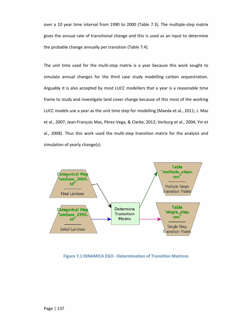
Page | 137

over a 10 year time interval from 1990 to 2000 (Table 7.3). The multiple-step matrix

gives the annual rate of transitional change and this is used as an input to determine

the probable change annually per transition (Table 7.4).

The unit time used for the multi-step matrix is a year because this work sought to

simulate annual changes for the third case study modelling carbon sequestration.

Arguably it is also accepted by most LUCC modellers that a year is a reasonable time

frame to study and investigate land cover change because of this most of the working

LUCC models use a year as the unit time step for modelling (Maeda et al., 2011; J. Mas

et al., 2007; Jean-François Mas, Pérez-Vega, & Clarke, 2012; Verburg et al., 2004; Yin et

al., 2008). Thus this work used the multi-step transition matrix for the analysis and

simulation of yearly change(s).

Figure 7.1 DINAMICA EGO - Determination of Transition Matrices

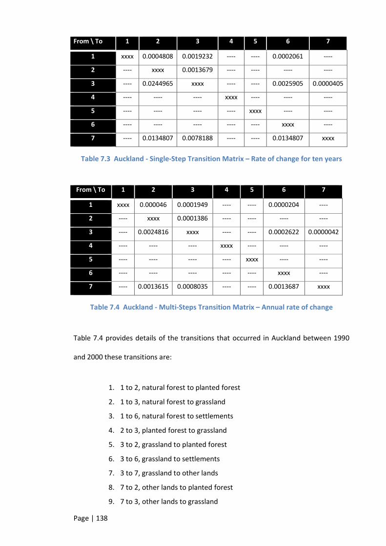
Page | 138

From \ To 1 2 3 4 5 6 7

1 xxxx 0.0004808 0.0019232 ---- ---- 0.0002061 ----

2 ---- xxxx 0.0013679 ---- ---- ---- ----

3 ---- 0.0244965 xxxx ---- ---- 0.0025905 0.0000405

4 ---- ---- ---- xxxx ---- ---- ----

5 ---- ---- ---- ---- xxxx ---- ----

6 ---- ---- ---- ---- ---- xxxx ----

7 ---- 0.0134807 0.0078188 ---- ---- 0.0134807 xxxx

Table 7.3 Auckland - Single-Step Transition Matrix – Rate of change for ten years

From \ To 1 2 3 4 5 6 7

1 xxxx 0.000046 0.0001949 ---- ---- 0.0000204 ----

2 ---- xxxx 0.0001386 ---- ---- ---- ----

3 ---- 0.0024816 xxxx ---- ---- 0.0002622 0.0000042

4 ---- ---- ---- xxxx ---- ---- ----

5 ---- ---- ---- ---- xxxx ---- ----

6 ---- ---- ---- ---- ---- xxxx ----

7 ---- 0.0013615 0.0008035 ---- ---- 0.0013687 xxxx

Table 7.4 Auckland - Multi-Steps Transition Matrix – Annual rate of change

Table 7.4 provides details of the transitions that occurred in Auckland between 1990

and 2000 these transitions are:

1. 1 to 2, natural forest to planted forest

2. 1 to 3, natural forest to grassland

3. 1 to 6, natural forest to settlements

4. 2 to 3, planted forest to grassland

5. 3 to 2, grassland to planted forest

6. 3 to 6, grassland to settlements

7. 3 to 7, grassland to other lands

8. 7 to 2, other lands to planted forest

9. 7 to 3, other lands to grassland

Page | 139

10. 7 to 6, other lands to settlements

These are the 10 transitions modelled for the Auckland Region. The transition rates

represent the net quantity of change, as the percentage of land that will change from

one state of land use/cover to another state. For example, the transition rate

0.0001386 (from states 2 to 3) indicates that 0.01386% of planted forest was lost to

grassland annually between 1990 and 2000. Like interest rates, the transition rates are

superimposed on the remaining stock of LUC annually. In this case there are 43,864

acres (see Table 6.3) of planted forest in 1990, then in 1991 there will be a loss of

0.01386% of 43,864 acres (6.08) to grassland leaving (43,864 – 6.08 = 43,857.02) acres

of planted forest. In 1992 there will be (43,857.02 - (43,857.02 * 0.0001386)) =

43850.94 acres of planted forest left.

7.1.2 Rondônia State

Using the same procedure (as applied to Auckland) the Rondônia LUC maps for the

years 1997 and 2000 were used to compute the single (Table 7.6) and multiple (Table

7.7) transitional matrices. Examining these two tables it’s obvious that only one

transition has occurred from forest to deforested land indicating deforestation. Table

7.6 reveals that from 1997 to 2000 almost 8.4% the Amazon forest of Rondônia was

lost and Table 7.7 indicates that the rate of deforestation was 2.88% annually. When

compared to the transitional rates in Auckland region this is a significant rate of

change.

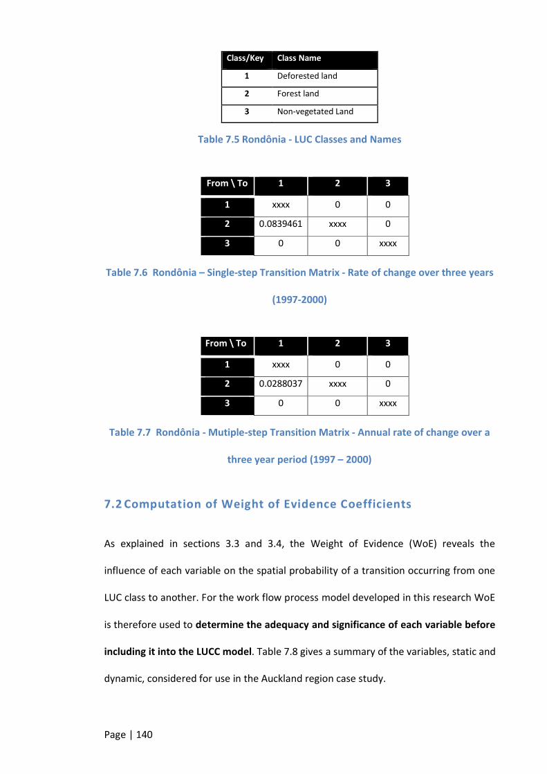
Page | 140


1 Deforested land

2 Forest land

3 Non-vegetated Land

Table 7.5 Rondônia - LUC Classes and Names

From \ To 1 2 3

1 xxxx 0 0

2 0.0839461 xxxx 0

3 0 0 xxxx

Table 7.6 Rondônia – Single-step Transition Matrix - Rate of change over three years

(1997-2000)

From \ To 1 2 3

1 xxxx 0 0

2 0.0288037 xxxx 0

3 0 0 xxxx

Table 7.7 Rondônia - Mutiple-step Transition Matrix - Annual rate of change over a

three year period (1997 – 2000)

7.2 Computation of Weight of Evidence Coefficients

As explained in sections 3.3 and 3.4, the Weight of Evidence (WoE) reveals the

influence of each variable on the spatial probability of a transition occurring from one

LUC class to another. For the work flow process model developed in this research WoE

is therefore used to determine the adequacy and significance of each variable before

including it into the LUCC model. Table 7.8 gives a summary of the variables, static and

dynamic, considered for use in the Auckland region case study.

Page | 141

Static Variables Dynamic Variables

Elevation Distance to natural forest

Slope Distance to planted forest

Hillshade Distance to grassland

Reserved lands Distance to cropland

Soil Distance to wetland

Distance to rivers Distance to settlements

Distance to major roads Distance to Other lands

Distance to minor roads

Table 7.8 List of Static and Dynamic Variables

The Weight of Evidence method employed in this work is only applicable to categorical

datasets/maps. Therefore all continuous grey scale variables for each case study were

categorised using the WoE Ranges tool (Figure 7.3) in DINAMICA (see section 3.3 for

details).

Static variables such as slope, elevation, distance-to-roads, distance-to-rivers and all

dynamic variables (distance-to-natural forest, distance-to-planted forest, distance-to-

grassland etc.) are continuous grey scale data. In order to be able to use the WOE

method to evaluate the adequacy and significance of these variables they must be

transformed into categorical data. The WoE ranges and coefficients calculation and

relevant parameters are shown in Figure 7.2 (see Figure 3.7 for sample results).

For each transition from LUC class k to l all the variables, both static and dynamic, were

applied to determine the WoE. The variables that showed no significant influence of

change on a specific land use/cover transition from class k to l were removed from the

set of variables; therefore each transition has a unique set of WoE coefficients of the

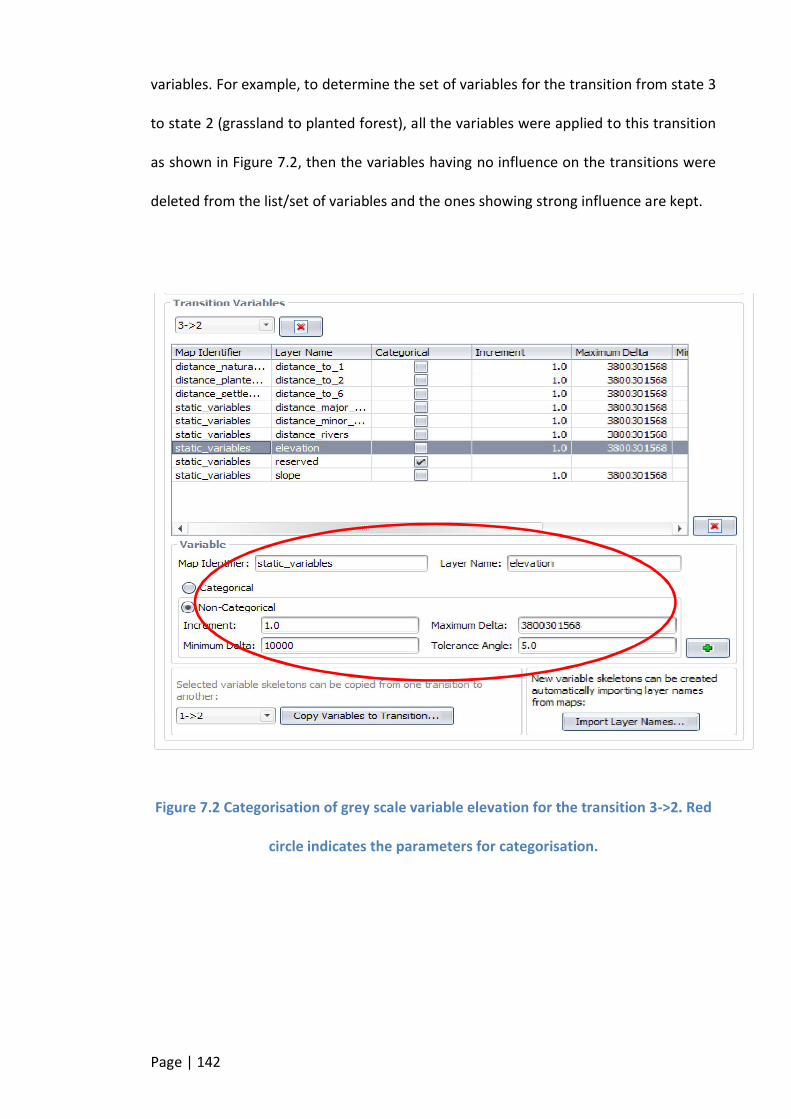
Page | 142

variables. For example, to determine the set of variables for the transition from state 3

to state 2 (grassland to planted forest), all the variables were applied to this transition

as shown in Figure 7.2, then the variables having no influence on the transitions were

deleted from the list/set of variables and the ones showing strong influence are kept.

Figure 7.2 Categorisation of grey scale variable elevation for the transition 3->2. Red

circle indicates the parameters for categorisation.

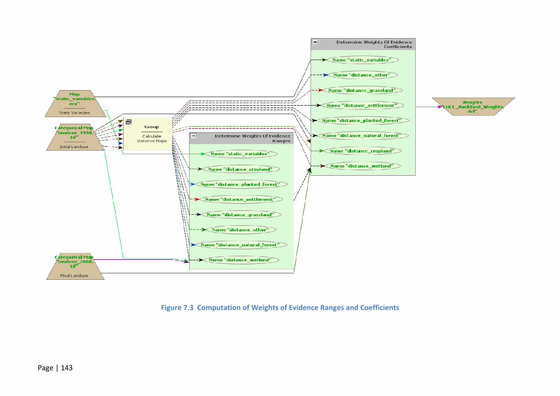
Page | 143

Figure 7.3 Computation of Weights of Evidence Ranges and Coefficients

Page | 144

Figure 7.4 is an excerpt from the results of WoE of the Auckland region variables,

showing that the variables which have a significant influence on the state transition from

state 3 to state 2, are flagged YES in the “Significant?” field. On the other hand Figure 7.5

shows that the variables distance-to-rivers and reserved lands had NO significant

influence on the transition from “1 to 2”. For this reason these two variables are omitted

from the modelling process for this transition.

Figure 7.4 Example of WoE of Variables showing Influence on transition

Page | 145

Figure 7.5 Example of WoE of Variables showing no influence on transition

Table 7.9 presents a summary of set of variables used for each of the transitions for the

Auckland Region, it is important to note that two variables, hillshade and soil, were not

included in any of the transitions because the WOE method proved that these variables

did not have any significant impact on the transitions to be included in the model.

Hillshading is the cast of sunlight on relief features (hills or valleys) and typically has a

significant impact on the degree of crop growth on specific areas due to sunlight. The

Hillshade variable had no influence on any of the transitions under investigation; this

Page | 146

could be due to the exclusion of the LUC type – cropland - which did not undergo change

in the 1990 to 2000 period.

The cells containing “red” ticks in Table 7.9 were not included in the LUCC model due to

their correlation with other variables. Variables are checked for correlation (see section

3.5) and if any variables are correlated one of them is removed and the other used. If

both are kept it causes double influence in a specific transitional change and will violate

the WoE assumption (see section 3.3.1).

Table 7.9 Summary of Variable List per Transition for Auckland LUCC Model

Variables\Transitions 1->2 1->3 1->6 2->3 3->2 3->6 3->7 7->2 7->3 7->6

Elevation

Slope

Hillshade

Reserved

Soil

Distance to Rivers

Distance to Major Roads

Distance to Minor Roads

Distance to 1(Natural Forest)

Distance to 2(Planted Forest)

Distance to 3(Grassland)

Distance to 4(Cropland)

Distance to 5(Wetland)

Distance to 6(Settlements)

Distance to 7(Other lands)

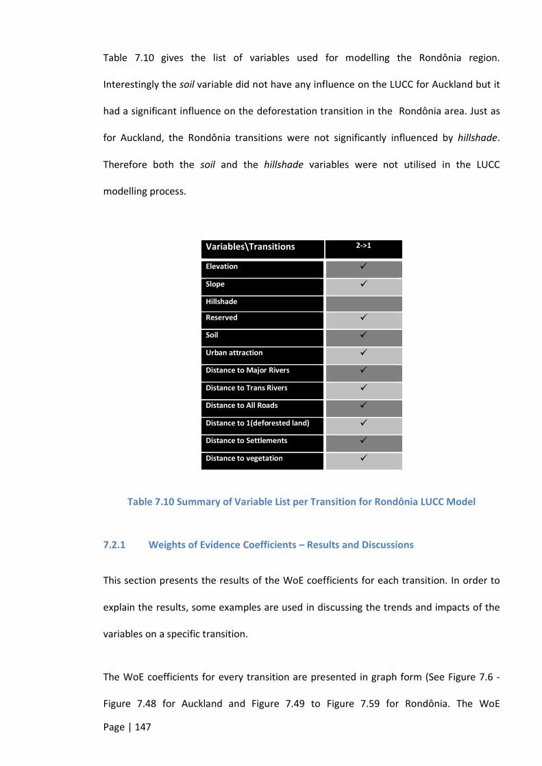
Page | 147

Table 7.10 gives the list of variables used for modelling the Rondônia region.

Interestingly the soil variable did not have any influence on the LUCC for Auckland but it

had a significant influence on the deforestation transition in the Rondônia area. Just as

for Auckland, the Rondônia transitions were not significantly influenced by hillshade.

Therefore both the soil and the hillshade variables were not utilised in the LUCC

modelling process.

Table 7.10 Summary of Variable List per Transition for Rondônia LUCC Model

7.2.1 Weights of Evidence Coefficients – Results and Discussions

This section presents the results of the WoE coefficients for each transition. In order to

explain the results, some examples are used in discussing the trends and impacts of the

variables on a specific transition.

The WoE coefficients for every transition are presented in graph form (See Figure 7.6 -

Figure 7.48 for Auckland and Figure 7.49 to Figure 7.59 for Rondônia. The WoE

Variables\Transitions 2->1

Elevation

Slope

Hillshade

Reserved

Soil

Urban attraction

Distance to Major Rivers

Distance to Trans Rivers

Distance to All Roads

Distance to 1(deforested land)

Distance to Settlements

Distance to vegetation

Page | 148

coefficients are shown on the vertical axes and the number of cells is shown on the

horizontal axes. Positive values of WoE favour a transition whilst negative values hinder

the transition.

For example, in Figure 7.9 within the range of 0 and 1320 cells there is a positive

coefficient however above 1320 the coefficient is negative. This means that cells within

the 0 to 1320 range for the variable “distance to planted forest” favour the transition

from natural forest to planted forest. For values above 1320 this transition is hindered.

This implies that within the buffer of 0 - 1320 cells from planted forest any Natural Forest

land parcel could change to planted forest whilst this transition is repelled beyond this

buffer.

Figure 7.31 is a graphical representation illustrating the influence of slope on the

transition from grassland to planted forest. This graph shows that of the transition from

grassland to planted forest (afforestation) is hindered when the range (in cells) of slope

(rise in degrees) is below 10 beyond this range afforestation of grassland is favoured.

Thus within the LUCC model for grassland in the slope range beyond 10 there is a

probability for this grassland to undergo afforestation.

7.2.1.1 Auckland Region

Transition 1-to-2, Natural Forest to Planted Forest: The graphs from Figure 7.6 to Figure

7.9 show the set of WoE coefficients for the variables which had a significant influence

on the transition from natural forest to planted forest in Auckland. Figure 7.6 and Figure

7.8 shows that natural forest LUC close to the geographic feature represented by these

variables (minor roads and settlements) is not found to undergo this transition to

planted forest. There is an optimal range of distances to each variable where natural

Page | 149

forest has a high affinity for change to planted forest. Beyond this range the impact of

the geographical feature (variable) on change reduces, for example where the distance

of natural forest to a minor road is between 0 and 260. The transition from natural forest

to planted forest is not observed whereas in at distances between 260 and 900. Figure

7.7 and Figure 7.9 reveal that natural forest LUC cover within the close vicinity of these

variables are most likely to have a LUC change to planted forest but the probability of

such as change gradually reduces as the distance from the variables increases.

Figure 7.6 Dist. to Minor Roads [1->2)

Figure 7.7 Dist. to Others

Figure 7.8 Dist. to Settlements

Figure 7.9 Dist. to Planted Forest

Transition 1-to-3, Natural Forest to Grassland: The WoE coefficients of the variables

from Figure 7.10 to Figure 7.17 show that all the significant variables except distance to

rivers (Figure 7.15) show a general trend where the likelihood of change is inversely

proportional to the distance from the variable. It is possible that such a trend does not

Page | 150

exist for the distance to rivers due to the environmental management practices in place

in the Auckland region.

Figure 7.10 Elevation [1->3]

Figure 7.11 Dist. to Grassland [1->3]

Figure 7.12 Dist. to Major Roads [1->3]

Figure 7.13 Dist. to Planted Forest [1->3]

Figure 7.14 Reserved Lands [1->3]

Figure 7.15 Dist. to Rivers [1->3]

Figure 7.16 Dist. to Settlements [1->3]

Figure 7.17 Slope [1->3]

Page | 151

Transition 1-to-6, Natural Forest to Settlements: For this transition only one variable,

Figure 7.18, showed significant evidence that natural forest lands close to settlements

have a high probability of changing to settlements and this decreases in probability with

increase in distance from settlements.


Transition 2-to-3, Planted Forest to Grassland: From the WoE coefficient of the

variables, Figure 7.19 to Figure 7.22, it can be seen that the transitional change from

planted forest-to-grassland has a general pattern of a higher probability that planted

forest may change grassland when close to the influencing variables than when they are

further apart. Only Figure 7.21, distance to other lands deviates from this trend. Given

that other lands is a variable that is comprised of all the minor LUC classes not explicitly

named in the data set due to their relatively small area or contribution to the region it is

not surprising that this variable influences LUC differently.

Figure 7.19 Dist. to Major Roads

Figure 7.20 Dist. to Natural Forest

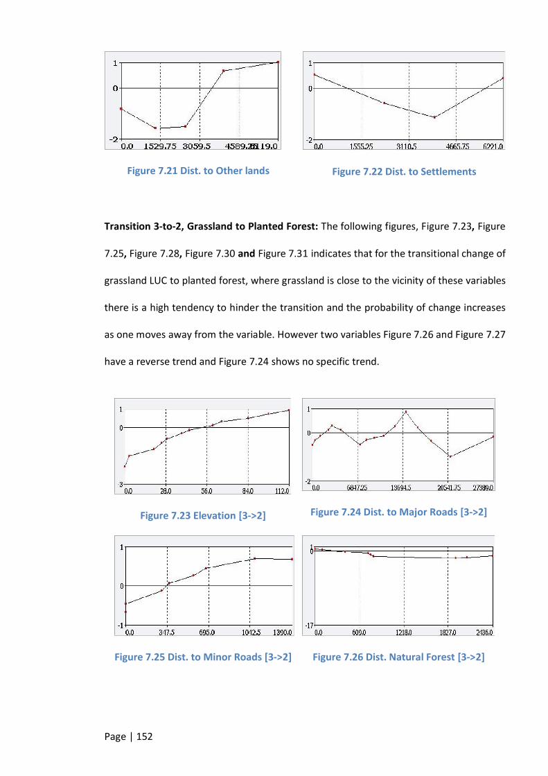
Page | 152

Figure 7.21 Dist. to Other lands

Figure 7.22 Dist. to Settlements

Transition 3-to-2, Grassland to Planted Forest: The following figures, Figure 7.23, Figure

7.25, Figure 7.28, Figure 7.30 and Figure 7.31 indicates that for the transitional change of

grassland LUC to planted forest, where grassland is close to the vicinity of these variables

there is a high tendency to hinder the transition and the probability of change increases

as one moves away from the variable. However two variables Figure 7.26 and Figure 7.27

have a reverse trend and Figure 7.24 shows no specific trend.



Figure 7.25 Dist. to Minor Roads [3->2]

Figure 7.26 Dist. Natural Forest [3->2]

Page | 153

Figure 7.27 Dist. to Planted Forest [3-

>2]

Figure 7.28 Reserved lands [3->2]




Transition 3-to-6, Grassland to Settlements: Figure 7.32 to Figure 7.41 shows the WoE

of the variable set and its influence transitional change from grassland to settlements. It

is obvious that there are two distinct patterns of influence of the variables; one category

reveals an increase in probability of this transitional change ranging from repulsion to

attraction (Figure 7.35 and Figure 7.39) whilst the reverse is true in the other category

(Figure 7.32, Figure 7.34, Figure 7.36, Figure 7.38, Figure 7.40 and Figure 7.41). The

others have no regular pattern.

Page | 154




Figure 7.35 Dist. to Natural Forest [3->6]

Figure 7.36 Dist. to Other [3->6]


Figure 7.38 Reserved lands [3->6]


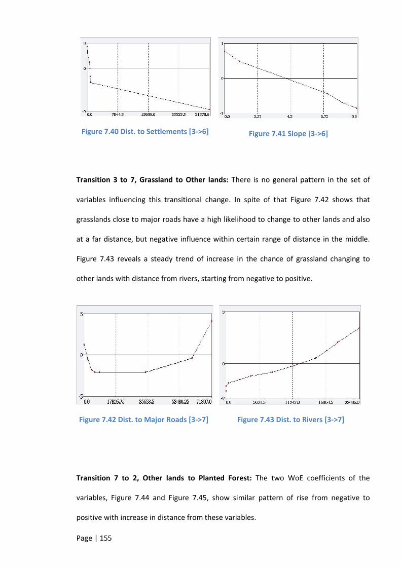
Page | 155



Transition 3 to 7, Grassland to Other lands: There is no general pattern in the set of

variables influencing this transitional change. In spite of that Figure 7.42 shows that

grasslands close to major roads have a high likelihood to change to other lands and also

at a far distance, but negative influence within certain range of distance in the middle.

Figure 7.43 reveals a steady trend of increase in the chance of grassland changing to

other lands with distance from rivers, starting from negative to positive.



Transition 7 to 2, Other lands to Planted Forest: The two WoE coefficients of the

variables, Figure 7.44 and Figure 7.45, show similar pattern of rise from negative to

positive with increase in distance from these variables.

Page | 156



Transition 7 to 3, Other lands to Grassland: This set of variables shows a remarkable

pattern of evidence in their influence in this transition because the two show the same

pattern.



Transition 7 to 6, Other lands to Settlements: Figure 7.48 reveals that other lands close

to settlements have a high chance of changing to settlements but this tendency reduces

with distance from settlements.

Page | 157


7.2.1.2 Rondônia State

As indicated in section 7.1.2 there is only one transition, deforestation, was considered

for Amazon forest zone of Rondônia state. For this transition 11 variables were found to

have a significant influence on the transition. Figure 7.49 to Figure 7.59 are the graphs of

WoE coefficients of the variables. With the exception of urban attraction (Figure 7.58)

and soil (Figure 7.57) the variables show a general trend of high level of deforestation of

forestlands that are very close to these variables but the trend decreases as the distance

increases.

Figure 7.49 Distance to deforested lands

Figure 7.50 Elevation

Page | 158

Figure 7.51 Distance to all roads

Figure 7.52 Distance to major rivers

Figure 7.53 Distance to settlements

Figure 7.54 Distance to trans-rivers

Figure 7.55 Protected areas

Figure 7.56 Slope

Figure 7.57 Soil

Figure 7.58 Urban Attraction

Page | 159

Figure 7.59 Vegetation

7.3 Analysing Correlation of Input Variables

To test the assumption in WoE that “the input variables are spatially independent”, the

pairwise testing (discussed in section 3.5) was used. For each transition the variable set

was tested for independence and if there is a high level of correlation between a pair

of variables one of them is deleted. Figure 7.60 presents the diagram of map

correlation in DINAMCA EGO, the tool “Determine Weights of Evidence Correlation”

takes in WoE Coefficients of the variables and maps of all the variables, the message

log displays the results of the pairwise tests displayed in the message log, as in Table

7.11.

Table 8.6 provides an excerpt showing the results of the variable comparison for

transitions 1-to-2 and 1-to-3. The first column is the first variable and the second

column the second variable and the other columns are the results of the test methods

(discussed in section 4.5). In this work for “Joint Information Uncertainty” (the last

column) values greater than 0.5 are flagged as having very high correlation and one of

Page | 160

the pair variables is therefore deleted. All the Joint Uncertainty values in Table 8.6 are

less than 0.2 showing weak correlation, thus acceptable.

After the map correlation analysis, the WoE Coefficients table is used as an input for

the LUCC model.

Figure 7.60 Determining Correlation of Variables

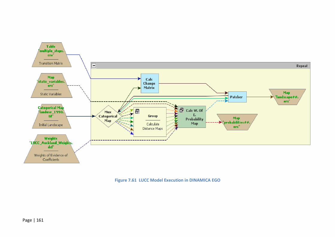
Page | 161

Figure 7.61 LUCC Model Execution in DINAMICA EGO

Page | 162

Transition: 1->2

Crammer Entropy

First Variable Second Variable Chi^2 Crammer* Contingency Joint Entropy Joint Uncertainity*

--------------------------------------------------------------------------------------------------------------------------------------------------------------------------------------------------------------------------------------------------------------------------

distance_other/distance_to_7 distance_planted_forest/distance_to_2 559553.5671 0.471603661 0.725621372 1.955349681 0.027590294

distance_other/distance_to_7 distance_settlement/distance_to_6 549645.6002 0.52257992 0.722544506 1.247168287 0.04421062

distance_other/distance_to_7 static_variables/distance_minor_roads 522591.7773 0.455761483 0.713768528 2.268815544 0.009432732

distance_planted_forest/distance_to_2 distance_settlement/distance_to_6 522163.5718 0.509348023 0.713625008 1.943463186 0.016694661

distance_planted_forest/distance_to_2 static_variables/distance_minor_roads 519540.7902 0.414835138 0.712742686 2.952389348 0.007853779

distance_settlement/distance_to_6 static_variables/distance_minor_roads 532926.6766 0.514570719 0.717187912 2.231462485 0.022356184

Transition: 1->3

Crammer Entropy

First Variable Second Variable Chi^2 Crammer* Contingency Joint Entropy Joint Uncertainity*

--------------------------------------------------------------------------------------------------------------------------------------------------------------------------------------------------------------------------------------------------------------------------

distance_grassland/distance_to_3 distance_planted_forest/distance_to_2 106234.5545 0.229744033 0.417521634 2.666182691 0.073617907

distance_grassland/distance_to_3 distance_settlement/distance_to_6 40538.5415 0.141920587 0.27305478 2.906053404 0.028348245

distance_grassland/distance_to_3 static_variables/distance_major_roads 57891.90147 0.169597813 0.321219836 3.300875127 0.03426445

distance_grassland/distance_to_3 static_variables/distance_rivers 34101.51404 0.130166183 0.251935119 3.384439553 0.018729816

distance_grassland/distance_to_3 static_variables/elevation 63213.89817 0.177253176 0.334131606 3.022821942 0.03692823

distance_grassland/distance_to_3 static_variables/reserved 4167.417672 0.245328901 0.238263559 1.714361119 0.034466867

distance_grassland/distance_to_3 static_variables/slope 32247.60101 0.126600798 0.245455611 3.102673198 0.019900367

distance_planted_forest/distance_to_2 distance_settlement/distance_to_6 543721.6201 0.367523102 0.72067062 3.515874171 0.023334152

distance_planted_forest/distance_to_2 static_variables/distance_major_roads 147158.0051 0.191200176 0.47569076 3.844752468 0.062098353

distance_planted_forest/distance_to_2 static_variables/distance_rivers 428644.6278 0.326321009 0.678239738 4.001618337 0.012100312

distance_planted_forest/distance_to_2 static_variables/elevation 42444.99272 0.118591986 0.278958336 3.652208192 0.020000594

distance_planted_forest/distance_to_2 static_variables/reserved 1524.65777 0.148388889 0.146781676 2.243569988 0.009916717

distance_planted_forest/distance_to_2 static_variables/slope 31817.06835 0.102676768 0.243909702 3.713760612 0.015766804

distance_settlement/distance_to_6 static_variables/distance_major_roads 50170.09846 0.105254957 0.301110034 4.096814787 0.024545181

distance_settlement/distance_to_6 static_variables/distance_rivers 459785.956 0.318638267 0.690993501 4.151608083 0.025741911

distance_settlement/distance_to_6 static_variables/elevation 99151.25446 0.167809994 0.405786647 3.76137688 0.055816397

distance_settlement/distance_to_6 static_variables/reserved 7046.493944 0.319008121 0.303918419 2.187865699 0.046624203

distance_settlement/distance_to_6 static_variables/slope 66910.74118 0.137853131 0.342646282 3.856044872 0.034402154

static_variables/distance_major_roads static_variables/distance_rivers 30193.65253 0.077463865 0.23792764 4.585142381 0.013505747

static_variables/distance_major_roads static_variables/elevation 26279.60038 0.086392908 0.222827322 4.25242484 0.012560352

static_variables/distance_major_roads static_variables/reserved 17270.62756 0.499423826 0.446801177 2.777661485 0.099933716

static_variables/distance_major_roads static_variables/slope 35483.96169 0.093905016 0.256703197 4.299371119 0.015737274

static_variables/distance_rivers static_variables/elevation 52090.62143 0.121632178 0.306336954 4.285819932 0.023684879

static_variables/distance_rivers static_variables/reserved 9867.729754 0.377505968 0.353178025 2.884825095 0.05108327

static_variables/distance_rivers static_variables/slope 30100.45764 0.086488684 0.237620361 4.361593713 0.013553486

static_variables/elevation static_variables/reserved 18222.35219 0.513159424 0.456555373 2.159462167 0.120599446

static_variables/elevation static_variables/slope 154544.1725 0.209505308 0.484802858 3.903394722 0.074949173

static_variables/reserved static_variables/slope 6476.205167 0.305921775 0.292538814 2.654893991 0.034888875

Table 7.11 Excerpt of Message log file - Correlation of Variables

7.4 Model Execution – Build and Run

After executing the processes of the calibration phase, the following outputs were

obtained:

multi-step transition matrix

WoE Coefficients of variables

In addition to these outputs the LUC map for t1 and static variable maps were used as

input data to set up and run the LUCC model (presented in Figure 7.61 and detailed in

section 4.6). In Figure 7.61 the direction of the arrows represents data flow and the

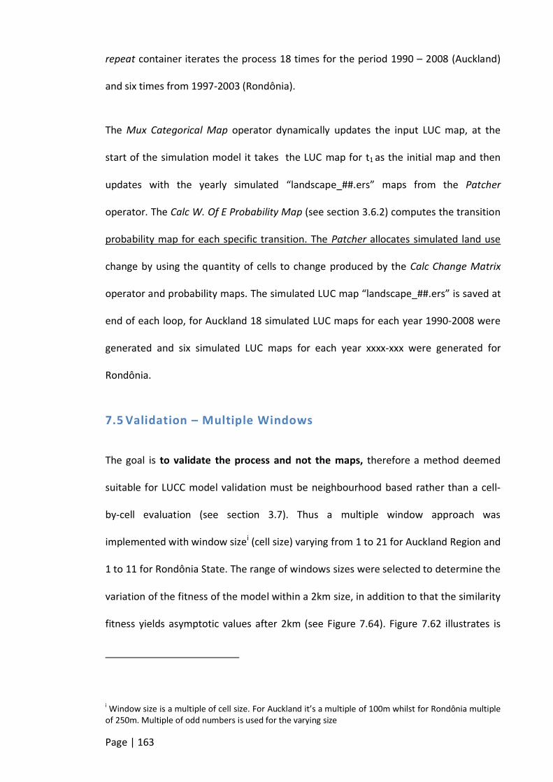
Page | 163

repeat container iterates the process 18 times for the period 1990 – 2008 (Auckland)

and six times from 1997-2003 (Rondônia).

The Mux Categorical Map operator dynamically updates the input LUC map, at the

start of the simulation model it takes the LUC map for t1 as the initial map and then

updates with the yearly simulated “landscape_##.ers” maps from the Patcher

operator. The Calc W. Of E Probability Map (see section 3.6.2) computes the transition

probability map for each specific transition. The Patcher allocates simulated land use

change by using the quantity of cells to change produced by the Calc Change Matrix

operator and probability maps. The simulated LUC map “landscape_##.ers” is saved at

end of each loop, for Auckland 18 simulated LUC maps for each year 1990-2008 were

generated and six simulated LUC maps for each year xxxx-xxx were generated for

Rondônia.

7.5 Validation – Multiple Windows

The goal is to validate the process and not the maps, therefore a method deemed

suitable for LUCC model validation must be neighbourhood based rather than a cell-

by-cell evaluation (see section 3.7). Thus a multiple window approach was

implemented with window sizei (cell size) varying from 1 to 21 for Auckland Region and

1 to 11 for Rondônia State. The range of windows sizes were selected to determine the

variation of the fitness of the model within a 2km size, in addition to that the similarity

fitness yields asymptotic values after 2km (see Figure 7.64). Figure 7.62 illustrates is

i Window size is a multiple of cell size. For Auckland it’s a multiple of 100m whilst for Rondônia multiple of 250m. Multiple of odd numbers is used for the varying size

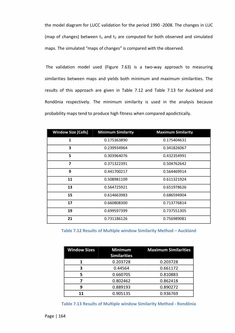
Page | 164

the model diagram for LUCC validation for the period 1990 -2008. The changes in LUC

(map of changes) between t1 and t2 are computed for both observed and simulated

maps. The simulated “maps of changes” is compared with the observed.

The validation model used (Figure 7.63) is a two-way approach to measuring

similarities between maps and yields both minimum and maximum similarities. The

results of this approach are given in Table 7.12 and Table 7.13 for Auckland and

Rondônia respectively. The minimum similarity is used in the analysis because

probability maps tend to produce high fitness when compared apodictically.

Window Size [Cells] Minimum Similarity Maximum Similarity

1 0.175363890 0.175404631

3 0.239934964 0.341826067

5 0.303964076 0.432354991

7 0.371322391 0.504762642

9 0.441700217 0.564469914

11 0.508981109 0.611321924

13 0.564725921 0.651978626

15 0.614663983 0.686594904

17 0.660808300 0.713776814

19 0.699597399 0.737551305

21 0.731186126 0.756989081

Table 7.12 Results of Multiple window Similarity Method – Auckland

Window Sizes Minimum Similarities

Maximum Similarities

1 0.203728 0.203728

3 0.44564 0.661172

5 0.660705 0.810883

7 0.802462 0.862418

9 0.889193 0.890272

11 0.905135 0.936769

Table 7.13 Results of Multiple window Similarity Method - Rondônia

Page | 165

Figure 7.62 Multiple Windows Validation

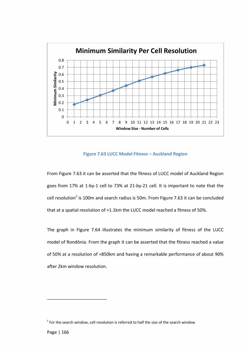
Page | 166

Figure 7.63 LUCC Model Fitness – Auckland Region

From Figure 7.63 it can be asserted that the fitness of LUCC model of Auckland Region

goes from 17% at 1-by-1 cell to 73% at 21-by-21 cell. It is important to note that the

cell resolutionii is 100m and search radius is 50m. From Figure 7.63 it can be concluded

that at a spatial resolution of ≈1.1km the LUCC model reached a fitness of 50%.

The graph in Figure 7.64 illustrates the minimum similarity of fitness of the LUCC

model of Rondônia. From the graph it can be asserted that the fitness reached a value

of 50% at a resolution of ≈850km and having a remarkable performance of about 90%

after 2km window resolution.

ii For the search window, cell resolution is referred to half the size of the search window

0

0.1

0.2

0.3

0.4

0.5

0.6

0.7

0.8

0 1 2 3 4 5 6 7 8 9 10 11 12 13 14 15 16 17 18 19 20 21 22 23

Min

imu

m S

imila

rity

Window Size - Number of Cells

Minimum Similarity Per Cell Resolution

Page | 167

Figure 7.64 LUCC Model Fitness – Rondônia Region

7.6 Enhancement of WoE Coefficients Using GA Tool

The WoE Coefficients are the main source of drivers of change in the LUCC model,

therefore the performance of the LUCC model depends on the WoE coefficients. In

order to improve the performance of the LUCC model in section 7.4 the GA tool

(described in Chapter 3) was used to enhance the WoE coefficients for optimal

“goodness of fit”. The performance of the deforestation LUCC model of Rondônia

(Figure 7.63) showed excellent results thus the GA was not applied to it but rather to

Auckland to find out if there could be an improvement. The GA tool sometimes “over

specialises” the WoE coefficients to yield the best “goodness of fit” but might not give

better projection into the future compared to the performance of the primal WoE

coefficients. To check for over specialisation, upper and lower boundaries (of 0%, 20%,

40%, 50%, 60%, 80%, 100% and 120%) were used and the GA tool used to run a range

0

0.1

0.2

0.3

0.4

0.5

0.6

0.7

0.8

0.9

1

0 1 2 3 4 5 6 7 8 9 10 11 12

Min

imu

m S

imila

rity


LUCC Model Fitness - Rondônia

Page | 168

of variations of the characteristics of the primal individual gene. After the search of the

optimal individual for the period 1990-2000, the individual set of coefficients was

validated. This was carried out for all the boundary limits. To determine which

boundary limit performed well, a comparative analysis of performances of the optimal

individuals (of the boundary limits) at both calibration and validation phases were run

and the best individual was selected.

The performance of the selected individual was then compared with the original set of

WoE coefficients (before GA calibration) and the one with better performance result

chosen as the optimal set of WoE coefficients to use in the work process flow model to

generate the LUCC projections.

Figure 7.65 illustrated the GA calibration model (executed in DINAMICA) and Figure

7.66 illustrates the GA Tool process.

The primal WoE coefficients (from Figure 7.6 to Figure 7.48) were converted into 47

tables (genes) of the WoE Coefficient which serves as input genes for the GA Tool

(Figure 7.65). The GA tool was configured as follows (see section 4.2):

Population size = 100

Convergence Stopping Criteria = 30 generations

Page | 169

Figure 7.65 GA Calibration Model - DINAMICA EGO

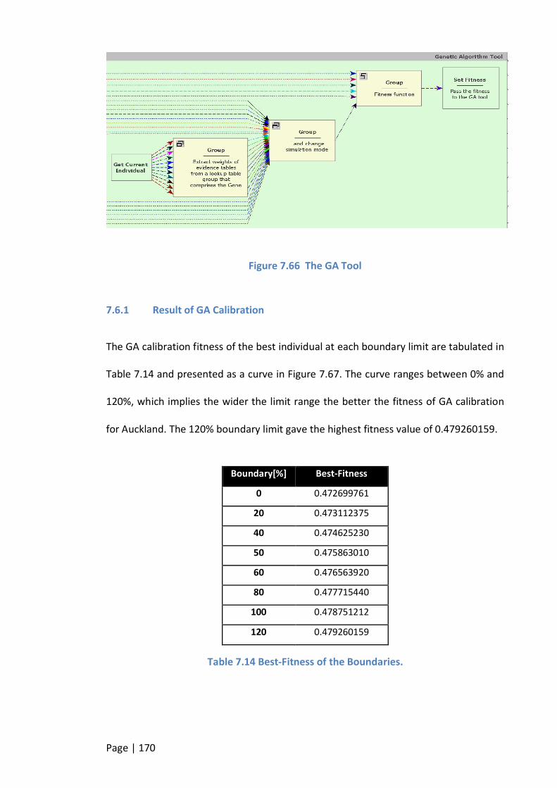
Page | 170

Figure 7.66 The GA Tool

7.6.1 Result of GA Calibration

The GA calibration fitness of the best individual at each boundary limit are tabulated in

Table 7.14 and presented as a curve in Figure 7.67. The curve ranges between 0% and

120%, which implies the wider the limit range the better the fitness of GA calibration

for Auckland. The 120% boundary limit gave the highest fitness value of 0.479260159.

Boundary[%] Best-Fitness

0 0.472699761

20 0.473112375

40 0.474625230

50 0.475863010

60 0.476563920

80 0.477715440

100 0.478751212

120 0.479260159

Table 7.14 Best-Fitness of the Boundaries.

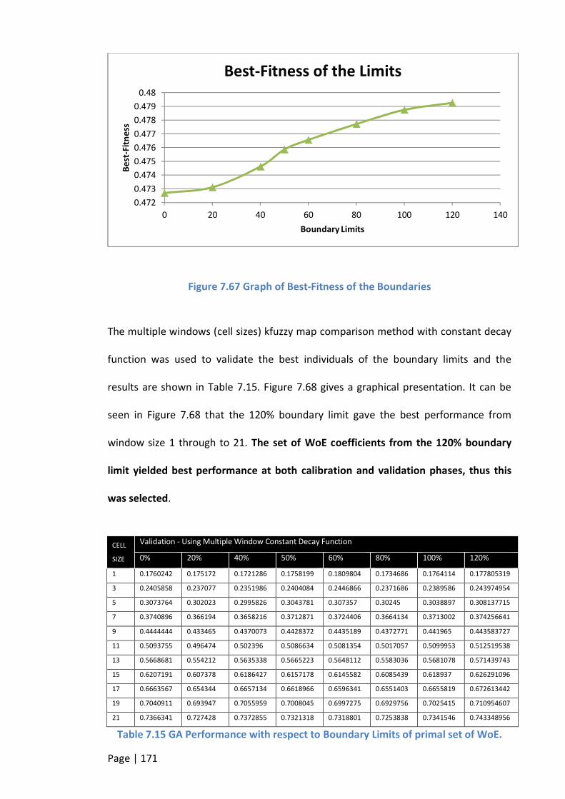
Page | 171

Figure 7.67 Graph of Best-Fitness of the Boundaries

The multiple windows (cell sizes) kfuzzy map comparison method with constant decay

function was used to validate the best individuals of the boundary limits and the

results are shown in Table 7.15. Figure 7.68 gives a graphical presentation. It can be

seen in Figure 7.68 that the 120% boundary limit gave the best performance from

window size 1 through to 21. The set of WoE coefficients from the 120% boundary

limit yielded best performance at both calibration and validation phases, thus this

was selected.

CELL

SIZE

Validation - Using Multiple Window Constant Decay Function

0% 20% 40% 50% 60% 80% 100% 120%

1 0.1760242 0.175172 0.1721286 0.1758199 0.1809804 0.1734686 0.1764114 0.177805319

3 0.2405858 0.237077 0.2351986 0.2404084 0.2446866 0.2371686 0.2389586 0.243974954

5 0.3073764 0.302023 0.2995826 0.3043781 0.307357 0.30245 0.3038897 0.308137715

7 0.3740896 0.366194 0.3658216 0.3712871 0.3724406 0.3664134 0.3713002 0.374256641

9 0.4444444 0.433465 0.4370073 0.4428372 0.4435189 0.4372771 0.441965 0.443583727

11 0.5093755 0.496474 0.502396 0.5086634 0.5081354 0.5017057 0.5099953 0.512519538

13 0.5668681 0.554212 0.5635338 0.5665223 0.5648112 0.5583036 0.5681078 0.571439743

15 0.6207191 0.607378 0.6186427 0.6157178 0.6145582 0.6085439 0.618937 0.626291096

17 0.6663567 0.654344 0.6657134 0.6618966 0.6596341 0.6551403 0.6655819 0.672613442

19 0.7040911 0.693947 0.7055959 0.7008045 0.6997275 0.6929756 0.7025415 0.710954607

21 0.7366341 0.727428 0.7372855 0.7321318 0.7318801 0.7253838 0.7341546 0.743348956

Table 7.15 GA Performance with respect to Boundary Limits of primal set of WoE.

0.472

0.473

0.474

0.475

0.476

0.477

0.478

0.479

0.48

0 20 40 60 80 100 120 140

Be

st-F

itn

ess

Boundary Limits

Best-Fitness of the Limits

Page | 172

Figure 7.68 Comparison of Boundary limits of GA Tool

7.7 Compare GA Calibration with the Primal WoE

The comparison of the GA result with the original (initial) WoE is to check if the GA

calibration process produced a better set of WoE coefficients. Table 7.16 and Figure

7.69 revealed that the WoEs coefficients generated from GA tool performed better

than the original set of coefficients however the improvement observed was minimal .

It was concluded the GA tool, for these case studies, enhanced the original WoE

coefficients. It is important to note that though GA could optimise the WoE

coefficients from t1 to t2 and yield very high fitness values, it is not always true that it

0.1

0.2

0.3

0.4

0.5

0.6

0.7

0.8

0 1 2 3 4 5 6 7 8 9 10 11 12 13 14 15 16 17 18 19 20 21 22

Min

imu

m S

imila

rity

Window SIze - Number of Cells

GA Performance of the Boundary Limits - Validation

0

20

40

50

60

80

100

120

Page | 173

will give high performance values during validation with t3 LUC (Soares-filho et al.,

2009).

Window Size Original GA

1 0.175363890 0.177805319

3 0.239934964 0.243974954

5 0.303964076 0.308137715

7 0.371322391 0.374256641

9 0.441700217 0.443583727

11 0.508981109 0.512519538

13 0.564725921 0.571439743

15 0.614663983 0.626291096

17 0.660808300 0.672613442

19 0.699597399 0.710954607

21 0.731186126 0.743348956

Table 7.16 Performance Comparison of Primal-WoE and GA-WoE

Figure 7.69 Performance Comparison of Original WoE and GA generated WoE

0

0.1

0.2

0.3

0.4

0.5

0.6

0.7

0.8

0 1 2 3 4 5 6 7 8 9 10 11 12 13 14 15 16 17 18 19 20 21 22 23

Min

imu

m S

imila

rity


Original WoE vs GA WoEOriginal

GA

Page | 174

7.8 LUCC Projected Simulation

After concluding the calibration and validation phases of the model process, the

selected coefficients were used to run a projected simulation from the year 1990 to

2050 for Auckland Region and from 1997 to 2018 for Rondônia. The simulation

projection for Auckland was designed to generate simulated base maps for carbon

sequestration (in order to demonstrate a further application of the LUCC model). For

Rondônia the projection was used largely to validate the model and compare it with

Auckland to ascertain the generic nature of the workflow process model. The output

formats were static and animatediii LUC simulated maps of each year.

The number of cells for each simulated LUC class for the years 1990, 2008, 2031 and

2050 for Auckland Region is presented in Table 7.17. The percentage of transitional

change with reference to 1990 LUC is shown in Table 7.18, where positive is equal to

percentage gain and negative is percentage loss. The quantified simulated cells per

LUC class for Rondônia can be seen in Table 7.19 and percentage change in Table 7.20.

These tables are graphically represented by Figure 7.70 and Figure 7.71 and show the

overall trend in LUCCs for Auckland and Rondônia respectively.

iii Animated video showing LUC maps from start year to end year of simulation.

Page | 175

LUC Classes Cell Count For

1990 2008 2031 2050

Natural Forest 145,587 144,903 144,029 143,307

Planted Forest 43,864 54,754 67,912 78,168

Grassland 247,056 235,782 222,200 211,633

Cropland 9,454 9,454 9,454 9,454

Wetland 3,825 3,825 3,825 3825

Settlements 49,678 50,962 52,524 53,740

Others 3,709 3,493 3,229 3,046

Table 7.17 Cell count of simulated LUC maps - Auckland

LUC Classes

Percentage of Change [%]

2008 2031 2050

Natural Forest -0.46982 -1.07015 -0.46982

Planted Forest 24.82674 54.824 24.82674

Grassland -4.56334 -10.0609 -4.56334

Cropland 0 0 0

Wetland 0 0 0

Settlements 2.584645 5.728894 2.584645

Others -5.82367 -12.9415 -5.82367

Table 7.18 Percentage of Simulated Change based on the 1990 LUC of Auckland.

Cell Count For

LUC Classes 1997 2000 2003 2006 2009 2012 2015 2018

Deforested 85,412 113,199 138,653 161,971 183,331 202,899 220823 237243

forest 331,010 303,223 277,769 254,451 233,091 213,523 195599 179179

Non-vegetation 26,501 26,501 26,501 26,501 26,501 26,501 26501 26501

Table 7.19 Cell count of simulated LUC maps – Rondônia

Percentage of Change [%]

LUC Classes 2000 2003 2006 2009 2012 2015 2018

Deforested 32.53 62.33 89.63 114.64 137.55 158.54 177.76

Natural forest -8.39 -16.08 -23.13 -29.58 -35.49 -40.91 -45.87

Non-vegetation 0 0 0 0 0 0 0

Table 7.20 Percentage of Simulated Change based on 1997 LUC map of Rondônia

In examining Figure 7.70, it can be concluded that cropland and wetland are constant

showing no change. The area of LUC attributed to grassland rapidly declining whilst

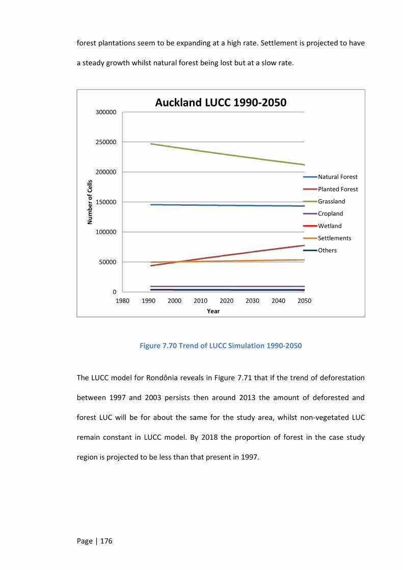
Page | 176

forest plantations seem to be expanding at a high rate. Settlement is projected to have

a steady growth whilst natural forest being lost but at a slow rate.

Figure 7.70 Trend of LUCC Simulation 1990-2050

The LUCC model for Rondônia reveals in Figure 7.71 that if the trend of deforestation

between 1997 and 2003 persists then around 2013 the amount of deforested and

forest LUC will be for about the same for the study area, whilst non-vegetated LUC

remain constant in LUCC model. By 2018 the proportion of forest in the case study

region is projected to be less than that present in 1997.

0

50000

100000

150000

200000

250000

300000

1980 1990 2000 2010 2020 2030 2040 2050

Nu

mb

er

of

Ce

lls

Year

Auckland LUCC 1990-2050

Natural Forest

Planted Forest

Grassland

Cropland

Wetland

Settlements

Others

Page | 177

Figure 7.71 The Trend of LUCC for the central Forest Region of Rondônia

The LUC maps in Figure 7.72 are sample maps of the simulation of LUCC model for

Rondônia. From the images it can easily be seen that time progresses there is an

increase in deforestation that is the forest LUC (green) decreases whilst the deforested

land (blue) increases.

Figure 7.83 Simulated LUC Maps 1991 and 2050 shows the simulated LUC maps of

1991 and 2050 put side by side to aid visualisation of Auckland LUCC between the two

maps. The amount of transitional LUCCs is very small and difficult to visualise from the

maps at such a scale. However, to present transitional changes in the maps, the areas

within the red boxes indicate some changes in LUC. For further illustration of

simulated LUC changes Figure 7.73 to Figure 7.82 shows the spatial distribution of each

of the ten LUC transitions from 1991 - 2050. The white patches depict the transitional

changes.

0

50,000

100,000

150,000

200,000

250,000

300,000

350,000

1995 2000 2005 2010 2015 2020

Ce

ll C

ou

nt

Year

Rondônia LUCC 1997 - 2018

Deforested

Natural forest

Non-vegetation

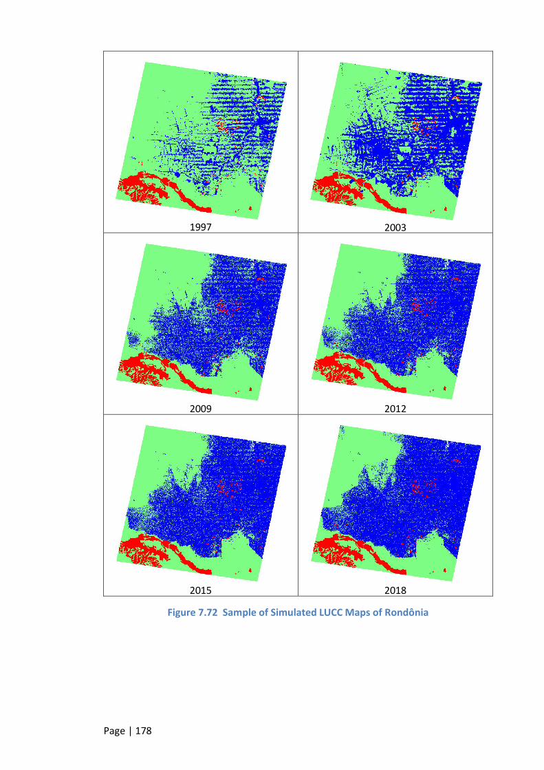
Page | 178

1997 2003

2009 2012

2015 2018

Figure 7.72 Sample of Simulated LUCC Maps of Rondônia

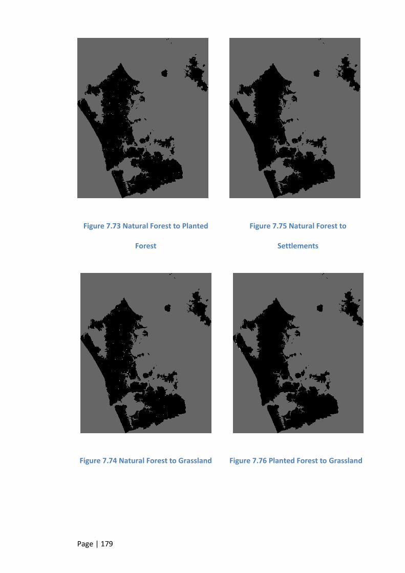
Page | 179

Figure 7.73 Natural Forest to Planted

Forest

Figure 7.74 Natural Forest to Grassland

Figure 7.75 Natural Forest to

Settlements

Figure 7.76 Planted Forest to Grassland

Page | 180

Figure 7.77 Grassland to Planted Forest

Figure 7.78 Grassland to Settlements

Figure 7.79 Grassland to Other lands

Figure 7.80 Others to Planted Forest

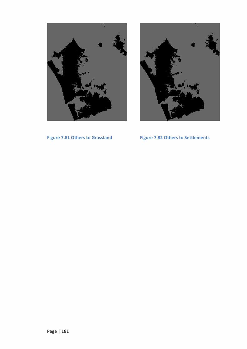
Page | 181

Figure 7.81 Others to Grassland

Figure 7.82 Others to Settlements

Page | 182

Figure 7.83 Simulated LUC Maps 1991 and 2050

New patches of Planted Forest formed

Grassland is still giving way to planted forest

The urban keeps on expanding

New patches of settlements

Forest plantation

growing gradually

New Stretch of Grassland developed

Page | 183

7.9 Scenario Description

Due to the changes in natural forest, planted forest and grassland (see Figure 7.70), it

seems prudent to assess the impact of such changes on greenhouse gases. Though

natural forest and grassland shows decline in area, planted forest shows significant

increase in land over the period. The Auckland region is an environmentally managed

region and it would be interesting to be able to demonstrate the effect of currently

policies such as infill housing on the level of carbon emissions. The goal of the third

case study presented, using the maps produced by the novel workflow process model

for Auckland, is to estimate the carbon sequestered annually by the vegetation based

on sequestration rates given by the New Zealand Ministry for Primary Industries,. The

sources of annual LUC map for the scenario model are the simulated maps from the

Auckland LUCC model, indicated in Figure 7.85 by a red bounding box. The scenario

model initially extracts natural forest, planted forest and grassland LUCs from the

simulated LUC map of each year, then computes the total number of cellsiv of each LUC

class multiplied by their respective carbon sequestration rate. This results in the

amount of carbon sequestered per LUC type for the year. The model repeats using a

time step of one year starting from the year 1990 through to 2050v. From the LUM

data used in this work plantation began in 1989, thus all planted forest were one year

old in 1990. When the right age of planted forest for 1990 is known the results can be

scaled by a factor.

iv Area of each cell is 100m by 100m = 1hectare

v Time frame given in Kyoto Protocol for assessing the performance of countries

Page | 184

Land Use/Cover Carbon Sequestration

Natural Forest 525tCO2/ha

Planted Forest 18tCO2/ha/yr.

Grassland 11tCO2/ha

Table 7.21 Carbon Sequestration Rates(Source: Ministry for Primary Industries, 2011)

Table 7.21 shows the sequestration rates used in this model, units measure tonnes of

carbon dioxide per hectare (tCO2/ha). It is important to note that the carbon

sequestration rate for the planted forest considers the age of the plant, which means if

the plantation is 6 years old it will be able to absorb (18*6)tCO2/ha.

Figure 7.84 Annual Carbon Sequestration by Vegetation

0

20000000

40000000

60000000

80000000

100000000

120000000

140000000

160000000

1980 1990 2000 2010 2020 2030 2040 2050 2060

Car

bo

n S

eq

ue

ste

red

[tC

O2

]

Year

Natural Forest

Planted Forest

Grassland

Total

Page | 185

Figure 7.85 Carbon Sequestration Scenario Model

LUC map from

LUCC MODEL

Page | 186

7.9.1 Results and Interpretation

The graph in Figure 7.84 shows the result of the carbon sequestration model. The

carbon sequestered by natural forest and grassland is decreasing slowly annually

however; this decrease seems to be compensated for by planted forest which has a

rapid increase in carbon stock. The shape annual increase in carbon stock of planted

forest can be accounted for by the afforestation and reforestation of natural forest and

grassland areas as seen in Auckland LUCC model.

The curve of the annual “total” carbon stock by the three LUCs indicates a steep rise

from 80MtCO2 in 1990 to about 144MtCO2 in 2050. “With all other things being

equal” and the past trend in change of LUC remains the same then projected

estimation of carbon stock annually will be similar to the graph.

It is worth mentioning that there might be other sources of carbon removal method

practices in Auckland but this work looked into only carbon removal by vegetation. It

could be said from Figure 7.84 that management of planted forest in Auckland Region

has made major contribution to removal of carbon dioxide from atmosphere. Also

from the same graph, even though sequestration from natural forest is decreasing

gradually it recorded the highest values of sequestration whilst grassland registered

the lowest figures.

7.10 Summary

In summary the workflow process (see Figure 3.1) was applied to Auckland and

Rondônia, and LUCC Model was achieved. Also the was shown that the simulated

Auckland LUC maps (red insert in Figure 7.85) can be used meaningfully in the context

Page | 187

of further modelling such as the presented carbon sequestration model. This shows

the applicability of the framework to more elaborate and extended LUCC based

studies.

The WoE method was initially used in calibrating the LUCC model for both study areas

and the WoE coefficients of Auckland were further improved using the GA method.

Using the WoE method the variables which had no significant influence on a specific

transition were removed thus for each specific transition the set of variables were

unique (see Table 7.9 and Table 7.10).

The performance of the LUCC model process was evaluated using the multiple

windows fuzzy map comparison method which yielded very good results for Auckland

region with fitness of over 51% at a window of 11-by-11 cell ( i.e. resolution of 550m)

to almost 75% at 21-by-21 cell window search (resolution 1,050m). For Rondônia the

process model gave an excellent performance result with fitness level of above 90% at

11-by-11 cell window search (resolution of 1,375m). Since the model performed well in

both study areas with varying location attributes it can be concluded that the workflow

process model is reasonably generic. Furthermore the model performed well in both

complex and simple LUC transitional changes with varying map resolutions; this

provides evidence that the model is able to project and simulate LUCC for very

spatially different areas and for scenarios of varying levels of complexity again

demonstrating not only the generic nature of the model developed in this research but

also the robustness of the model.

Page | 188

Chapter 8 Conclusions and Recommendations

This chapter briefly summaries the contributions to existing knowledge and findings of

this doctoral research. The limitations of the work are discussed and recommendations

are made for future research in the domain of LUCC modelling.

The research, reported in this thesis, involved and in depth investigation of existing

LUCC models and modelling methods. As a result of this investigation it was concluded

that there was a need for a generic integrated-working-process for LUCC modelling.

The research also attempted to answer the major question, “how can we measure the

'adequacy' of the components, variables and parameter sets, which combine to inform

the development of an LUCC model?” and the adequacy of these variables was then

evaluated using the novel LUCC process model developed as part of this work. The

WoE method reported in sections 3.3 and 3.4 was proven to be a successful method

for measuring the adequacy and significance of variables. The performance of the

derived integrated-working-process model was evaluated by applying it to the

Auckland Region case study from which an advanced model of carbon sequestration

was subsequently developed. The following are the key findings and deductions that

arose as a result of this research:

8.1.1 Investigation of LUCC Modelling Methods

It was found that GIS and RS techniques have the capability to detect LUCC (see

section 2.7). However, these techniques are limited when it comes to answering

Page | 189

questions about WHY the change occurred. One of the strengths of LUCC modelling is

that such a model is able to answer the WHY questions.

Three categories of LUCC modelling methods were investigated (i) statistics (ii) CA and

(iii) ABM or Multi-agent Systems (see section 2.8). Each of these methods has

strengths and weaknesses. CA uses cells which are spatially interconnected as

automata and each cell state is updated every discrete time step according to a set of

predefined rules. Therefore, CA is suitable for simulating LUC as they change. In this

research CA was selected in combination with statistics, in order to draw on the

strengths of both methods, to determine the transition matrix and WoE coefficients of

variables of each LUC transition.

The CA approach was limited because it does not allow the introduction or inclusion of

mobile agents for change such as human beings. Since the properties of raster CA does

not accommodate mobile agents an integration of the three LUCC modelling methods

– statistical, CA and ABM – will be valuable to LUCC modelling.

8.1.2 Review of CA LUCC Models/Software

Even though there are many working CA LUCC models most of them were designed for

binary LUC transition simulation or urban growth, however, SLEUTH, LEAM and

MOLAND do have the capability to simulate complex LUCC. These models were

originally designed with parameters for specific locations; therefore modellers are

unable to introduce new parameters into these models to even determine their

“adequacy” for causing change in LUC, users can only change the coefficients of

parameters during calibration to suite new locations.

Page | 190

In section 2.9, DINAMICA EGO was found to be a CA modelling platform, but not a

model, that integrates all the tools required to implement any of the existing LUCC

model and environmental modelling tasks. DINAMICA EGO gives user the freedom to

introduce variables and determine the significance of those variables. The generic

workflow process model developed in this research was successful implemented in

DINAMICA and it evaluated using two study areas.

8.1.3 LUCC Working Processes

Step-by-step integrated working processes (see Figure 3.1) for LUCC modelling was

derived from a unique combination of DINAMICA EGO and SLEUTH processes. This

novel work flow process model was successfully applied to Auckland Region and

Rondônia State and its performance evaluated. The model performed very well in both

simple and complex transitional LUCC (see section 7.5). An advanced scenario model of

vegetative carbon sequestration based on Auckland LUCC was implemented, this is an

instance indicating that a complex LUCC could be developed from the workflow

process model and used for further studies.

The Weights of Evidence method, Bayesian approach, was successfully used to

measure the adequacy and significance of each variable before including into the LUCC

model. This WoE method has an advantage over other statistical methods, such as

Logistic and Linear Regression, because it is not constrained by statistical assumptions

of parametric methods which violate spatial data. In section 3.3, the effect of each

variable on a specific transition was computed independently of the combined

solution, so that the WoE represents the variable’s influence on a single specific

transition.

Page | 191

The evaluation of the performance of the variables for each transition revealed that

each transition has a unique set of variables influencing it (see Table 7.9 and Table

7.10). Furthermore, the trend of influence of each variable in any specific transition

was found to be unique, for example distance-to-major roads is unique each transition

it had influence on (see Figure 7.6 to Figure 7.59). This remarkable result was

anticipated because each transitional change is unique therefore each variable

influence should be unique per transition.

8.1.4 Validating Maps versus Validating Model process

In LUCC modelling, typically map comparison methods are usually used to validate two

maps A and B, where A is the observed map and B is the simulated map. However, a

better is to evaluate the simulation process rather than the maps. In order to evaluate

a simulation process, the reference process of change is compared with the simulated

one for the same time period. Process of change is the transition that has occurred in

an area between time t1 and t2, resulting in a “map of change” (i.e. changes between

map[t1] and map[t2]). Thus the observed-map-of-change is compared with the

simulated-map-of-change to evaluate the performance of the simulation model. In this

research the simulation process if change itself was evaluated.

8.1.5 Qualitative vs. Quantitative Validation

The qualitative visual inspection (of maps by a human observer (expert) usually reveals

interesting characteristics – such as local similarities, global similarities, logical

coherence and patterns – and to the best of my knowledge performs better than the

mathematical procedures (here in described as quantitative) for validating small area

maps. However, mathematical procedures are preferred to visual inspection when the

Page | 192

area/map is large and with too much information because of the time required to

undertake a qualitative evaluation.

It was found that the mathematical procedures using a cell-by-cell approach does not

consider the similarities of LUC patterns on regional scale which a visual inspection

could capture. Additionally, current automated validation methods such as multiple

fitting window, hierarchical fuzzy and KFuzzy (kappa and fuzzy) similarity attempt to

resolve the issue of spatial pattern using vicinity based comparison rather than cell-by-

cell (see section 3.7). Whilst the multiple window similarity method considers spatial

pattern when quantifying the similarities between two maps the cell-by-cell approach

does not, thus is approach resolves the limitations regarding visual inspection and cell-

by-cell.

8.1.6 Validation Method

Section 6.3 reports on the rasterisation of the 1990 and 2008 LUC maps from vector

based LUC data using a 100m resolution. The vector-to-raster method used usually

determines which LUC class to assign to cells that lie along the boundary of two LUC

types. This raises data integrity concerns (boundary precision), despite the

preservation of spatial patterns. For example during the vector-to-raster conversion

along the boundary of the natural forest and grassland LUC, a cell assigned natural

forest may overlap the grassland area in the vector data. The conversion methods

usually capture the pattern of LUC area and not the exact boundaries, in view of this it

was deemed appropriate to use Kappa and Fuzzy similarity comparisons to validate the

spatial pattern.

Page | 193

A vector based CA approach would have been suitable but because all the input

datasets were in raster format this approach was explored.

8.1.7 Auckland Data Issues

Three LUC maps -1990, 2000 and 2008 – were used for this work. As mentioned in

section 8.1.6 the integrity of the data for 1990 and 2008 on the boundaries is uncertain

due to the vector-to-raster conversion method. On the other hand, the 2000 LUC map

was acquired and prepared using a GIS and RS procedure detailed in section 2.4. This

approach also has its own inherent errors (e.g. as a result of incorrect image

classification). Thus the error introduced in 1990 and 2008 LUC maps could be

different from errors in 2000 map. This was of concern because of a potential lack of

temporal data consistency, a 2000 LUC map derived from the same source as the 1990

and 2008 would have been more suitable and minimised the level of error introduced

by the data harmonisation process.

Although there might some data issues for the Auckland case study the goal this

research is to test the performance of LUCC workflow process model using real study

areas. Data for real study areas have never being perfect so measuring the

performance of the system on a clean dataset is not realistic. Therefore the model

executes based on input data and the assumption is that the data is “correct”.

As mentioned in section 6.2 the data for Rondônia State was provided by CSR and used

for their successful projects, therefore it was assumed that data integrity was good

enough for this project. However due to the low spatial resolution (250m) of the data

Powell et al. (2004) report that there are mixed pixels along the boundary of two

Page | 194

classes. Again, the application to Rondônia State performed well, thus data issues did

not have significant impact on the performance of the model.

8.1.8 Calibration and Performance of the LUCC Model

After the computation of transition matrix in section 7.1, it was found out that

cropland and wetland in Auckland Region remained unchanged between 1990 and

2000. This was indeed a remarkable finding because the assumption was that all the

LUC classes have undergone change.

In section 7.2 the WoE method was applied successfully resulting in the WoE

coefficients of the variable set for LUCC. In order to find out whether or not a GA could

improve the performance of the WoE coefficients in LUCC simulation model, the GA

tool was applied to the prime WoE coefficients using various boundary limits (see

section 7.6). It was found that for the Auckland Region the 120% boundary limit

performed the best (see section 7.7). It is worth noting that other boundary limits, for

instance 100% or 50%, might perform better in other locations or with a different

variable set for the same LUC transition.

The generic nature of the workflow process was tested by using the model to

undertake two case studies. The case studies were selected to demonstrate the

applicability of the model to modelling scenarios where the data informing the

modelling process is very different. It was found that the model performed well:

in both simple and complex LUCC transitional changes, however it performed

better with simple LUCC transition (with only one transition). The complex

LUCC model involved ten transitions and the overall error is the total of the

errors in each transition. The goodness of fit performance of the model

Page | 195

reached 50% at a resolution of 1.1km for Auckland (the complex transitions)

and 0.85km for Rondônia (see section 7.5).

over different rates of LUCC - the rate of LUCC, Auckland’s change was slower

than Rondônia’s (see Table 7.4 for Auckland and Table 7.7 for Rondônia)

with different map resolutions - for Auckland the spatial resolution was 100m

and for Rondônia 250m.

with very large area extents, 1,915,281ha for Auckland and 3,824,150ha

Rondônia.

These results showed that the workflow process model is generic and can be applied

to study areas with varying level of transitional complexity and with a wide variety of

dataset attributes.

For the Auckland Region, the GA set of coefficients performed better than the prime

WoE coefficient when a comparative analysis of the two sets was carried out.

Therefore it was concluded that for Auckland Region GA calibration was able to

enhance the coefficients of WoE method. For Rondônia study area, the prime WoE

coefficients performance in LUCC was excellent (see Figure 7.64), therefore the GA tool

was used to improve their performance.

8.2 Limitations of this Work

Although this research was carefully prepared and has reached the set goals (see

section 1.1), there are a number of limitations.

First of all due to limited availability of data, the calibration period of 1990-2000 for

the Auckland region and 1997-2000 for Rondônia state, were not long enough to

capture adequate empirical change for longer projection, a wider time range of

empirical datasets would have been more appropriate.

Page | 196

Secondly, the multiple transition matrices and change rates were based on the

assumption of section 3.2.1 that the transition rates per year are uniform for the

calibration period, which in reality is not true, and this could introduce an error. Such

errors could be minimised if there are more empirical LUC maps introduced for the

calibration period, for instance t1-t2-t3-t4 instead of t1-t2 used in this work, to capture

the variations in the transition rates rather than assuming uniformity.

8.3 Contribution

The contribution and significance of this thesis to the existing body of knowledge in

field of geosimulation and land use cover simulation is:

An effective WoE method for determining the adequacy and significance of

LUCC variables by applying it to Auckland.

a generic integrated-work-flow-process for LUCC modelling.

8.4 Future Work

As mentioned in section 8.2 the available empirical spatio-temporal LUC maps were

limited. To further enhance the work done in this thesis regarding the evaluation

performance of the workflow process a future work could include the following:

1. Increasing the number of empirical LUC maps for calibration and validation, at

least five of them at times t1, t2, t3, t4 and t5. Where t1, t2 and t3 could be

used for calibration and another three set t1, t4 and t5 for validation.

2. Using LUC maps covering larger extent, for example national maps since this

work was done on a regional level.

Page | 197

This research used a combination of statistical and cellular automata because the focus

was to simulate the LUCC and not the agents. For future work an incorporation of

agent base modelling method or tight coupling of the three methods into the LUCC

workflow process model will aid modellers to include mobile agents and other

socioeconomic variables and to visualise their effects on LUCC.

8.5 Conclusion

In conclusion LUCC modellers could adopt the novel and generic integrated workflow

process model developed as a result of this doctoral research to investigate the

parameters that are driving changes in any locality or region. Such an investigation

could serve as an input into the decision making process and assist stakeholders with

the development and implementation of LUC policy. Also LUCC modellers could use

this workflow process for building LUCC model frameworks for further investigation

and projections of the impact of LUCC.

Page | 198

REFERENCES

Agarwal, C., Green, G. M., Grove, J. M., Evans, T. P., & Schweik, C. M. (2002). A review and assessment of land-use change models: dynamics of space, time, and human choice. Retrieved from http://www.geog.ucsb.edu/~kclarke/ucime/Helens-Sem/seminar2001/Land_Use_Draft_9.pdf

Agterberg, F. P., & Bonham-Carter, G. F. (1990). Deriving weights of evidence from geoscience contour maps for the prediction of discrete events. In XXII International Symposium AP-COM (pp. 381–395).

Al-ghamdi, K. A. (2012). Modeling Spatial Dynamics Changes with Cellular Automata, 1–7.

Almeida, M., Lacerda, L., Bastos, W., & Herrmann, J. (2005). Mercury loss from soils following conversion from forest to pasture in Rondonia, Western Amazon, Brazil. Environmental Pollution, (137), 179–186.

Anderson, R, J., Hardy, E. E., Roach, J. T., & Witmer, R. E. (1976). A Land Use And Land Cover Classification System For Use With Remote Sensor Data. Washington.

Bellinger, G. (2004). Modeling & Simulation : An introduction. Retrieved October 10, 2010, from http://www.systems-thinking.org/modsim/modsim.htm

Benenson, I., & Torrens, P. M. (2004). Geosimulation : Automata-based modelling of urban phenomena (p. 287). West Sussex: Wiley.

Bonham-Carter, G. (1994). Map Pairs. In Geographic Information Systems for Geoscientists: Modelling With Gis (pp. 221–266). Pergamon. Retrieved from http://books.google.co.nz/books?id=7OMiShJX0wAC

Bowman, M. S., Soares-Filho, B. S., Merry, F. D., Nepstad, D. C., Rodrigues, H., & Almeida, O. T. (2012). Persistence of cattle ranching in the Brazilian Amazon: A spatial analysis of the rationale for beef production. Land Use Policy, 29(3), 558–568. Retrieved from http://www.sciencedirect.com/science/article/pii/S0264837711001037

Bremner, D., Demaine, E., Erickson, J., Iacono, J., Langerman, S., Morin, P., & Toussaint, G. (2005). Output-Sensitive Algorithms for Computing Nearest-Neighbour Decision Boundaries. Discrete & Computational Geometry, 33(4), 593–604 LA – English. doi:10.1007/s00454-004-1152-0

Carlson, K. M., Curran, L. M., Ratnasari, D., Pittman, A. M., Soares-Filho, B. S., Asner, G. P., … Rodrigues, H. O. (2012). Committed carbon emissions, deforestation, and community land conversion from oil palm plantation expansion in West

Page | 199

Kalimantan, Indonesia. Proceedings of the National Academy of Sciences of the United States of America, 109(19), 7559–64. doi:10.1073/pnas.1200452109

Chen, D., & Stow, D. (2002). The Effect of Training Strategies on Supervised Classification at Different Spatial Resolutions. Photogrammetric Engineering & Remote Sensing, 68(11), 1155–1161.

Cingolani, A. M., Renison, D., Zak, M. R., & Cabido, M. R. (2004). Mapping vegetation in a heterogeneous mountain rangeland using landsat data: an alternative method to define and classify land-cover units. Remote Sensing of environment, 92(1), 84–97.

Clarke, K. C. (1986). Advances in geographic information systems. Computers, Environment and Urban Systems, 10(3-4), 175–184.

Clarke, K. C. (2012). PROJECT GIGALOPOLIS - SLEUTH. Retrieved September 11, 2012, from http://www.ncgia.ucsb.edu/projects/gig/

Clarke, K. C., & Goldstein, N. C. (n.d.). A Decade of SLEUTHing : Lessons Learned from Applications of a Cellular Automaton Land Use Change Model.

Costanza, R. (1989). Model goodness of fit: A multiple resolution procedure. Ecological Modelling, 47(3–4), 199–215. Retrieved from http://www.sciencedirect.com/science/article/pii/030438008990001X

Couclelis, H. (1987). Cellular dynamics: How individual decisions lead to global urban change. European Journal of Operational Research, 30(3), 344–346. Retrieved from http://www.sciencedirect.com/science/article/pii/0377221787900804

Couclelis, H. (2001). CA and AbS are close cousins.

De Almeida, C. M., Batty, M., Vieira Monteiro, A. M., Câmara, G., Soares-Filho, B. S., Cerqueira, G. C., & Pennachin, C. L. (2003). Stochastic cellular automata modeling of urban land use dynamics: empirical development and estimation. Computers, Environment and Urban Systems, 27(5), 481–509. Retrieved from http://www.sciencedirect.com/science/article/pii/S019897150200042X

Deadman, P., Brown, R. D., & Gimblett, H. R. (1993). Modelling Rural Residential Settlement Patterns with Cellular Automata. Journal of Environmental Management, 37(2), 147–160. Retrieved from http://www.sciencedirect.com/science/article/pii/S030147978371011X

Demorgraphia. (2012). Demographia World Urban Areas ( World Agglomerations). Demorgraphia.

Dietzel, C., & Clarke, K. C. (2007). Research Article Toward Optimal Calibration of the SLEUTH Land Use Change Model. Transactions in GIS, 11(1), 29–45.

Dymond, J. R., & Shepherd, J. D. (2004). The spatial distribution of indigenous forest and its composition in the Wellington region, New Zealand, from ETM+ satellite

Page | 200

imagery. Remote Sensing of Environment, 90(1), 116–125. doi:10.1016/j.rse.2003.11.013

Eastman, J. R. (2003). IDRISI Kilimanjaro Guide to GIS and Image Processing. Worcester, MA.

Eastman, J. R., Van Fossen, M. E., & Solorzano, L. A. (2005). Transition Potential Modeling for Land Cover CHange. In D. Maguire, M. Batty, & M. Goodchild (Eds.), GIS, Spatial Analysis and Modeling (pp. 357–386). Redland, California: Esri Press.

Economist Intelligent Unit. (2012). The Liveabililty Ranking and Overview August 2012. The Economist. Retrieved from https://www.eiu.com/public/topical_report.aspx?campaignid=Liveability2012

Ellis, E., & Pontius, R. (2010). Land-use and land-cover change. In Encyclopedia of Earth. doi:April 18, 2010

Environment European Agency, E. (1984). CORINE land cover - contents. Retrieved from http://www.eea.europa.eu/publications/COR0-landcover/land_cover.pdf

Feddema, J., Oleson, K., Bonan, G., Mearns, L., Buja, L., Meehl, G., & Washington, W. (2005). The Importance of Land-Cover Change in Simulating Future Climates. Science, 310(5754), 1674–1678.

Fisher, P., & Unwin, D. J. (2005). Re-presenting GIS. (P. Fisher & D. J. Unwin, Eds.) (pp. 85–98). London.

Gibb, A., St-Jacques, J.-C., Nourry, G., & Johnson, T. (2002). A Comparison of Deterministic vs Stochastic Simulation Models for Assessing Adaptive Information Management Techniques over Disadvantaged Tactical Communication Networks.

Giudice, R., Soares-Filho, B. S., Merry, F., Rodrigues, H. O., & Bowman, M. (2012). Timber concessions in Madre de Dios: Are they a good deal? Ecological Economics, 77(0), 158–165. Retrieved from http://www.sciencedirect.com/science/article/pii/S0921800912000882

Goodacre, A. K., Bonham-Carter, G. F., Agterberg, F. P., & Wright, D. F. (1993). A statistical analysis of the spatial association of seismicity with drainage patterns and magnetic anomalies in western Quebec. Tectonophysics, 217(3–4), 285–305. Retrieved from http://www.sciencedirect.com/science/article/pii/0040195193900118

Gregorio, A. Di, & Jansen, L. J. M. (2005). LAND COVER CLASSIFICATION SYSTEM: Classification concepts and use manual. Rome. Retrieved from http://www.fao.org/gtos/doc/ECVs/T09/ECV-T9-landcover-ref25-LCCS.pdf

Grubb, M. (2004). Kyoto and the Future of International Climate Change Responses : From Here to Where ? International Review of Environmental Strategies, 5(1), 1–24.

Page | 201

Guan, Q., & Clarke, K. C. (2010). A general-purpose parallel raster processing programming library test application using a geographic cellular automata model. International Journal of Geographical Information Science, 24(5), 695–722. doi:10.1080/13658810902984228

Guizani, M., Rayes, A., Khan, B., & Al-Fuqaha, A. (2010). Basic Concepts and Techniques. In Network Modeling and Simulation : A Practical Perspective (1st ed., pp. 1–65). Wiley-Interscience.

Guo, Y. T. and P., & Lyu, M. R. (2005). Comparative Studies on Feature Extraction Methods for Multispectral Remote Sensing Image Classification. In IEEE International Conference on Systems, Man and Cybernetics (pp. 1275–1279). Waikoloa, Hawaii.

Hagen, A. (2003). Fuzzy set approach to assessing similarity of categorical maps. International Journal of Geographical Information Science, 17(3), 235–249. doi:10.1080/13658810210157822

Hopkins, L. D. (1999). Structure of a planning support system for urban development. Environment and Planning B: Planning and Design, 26(3), 333–343. Retrieved from http://www.envplan.com/abstract.cgi?id=b260333

Hu, G., & Xie, Y. (2006). An Extended Cellular Automata for Data Mining of Land Development Data. In 5th IEEE/ACIS International Conference on Computer and Information Science.

Huang, J., Zhang, J., & Lu, X. X. (2008). APPLYING SLEUTH FOR SIMULATING AND ASSESSING URBAN GROWTH SCENARIO BASED ON TIME SERIES TM IMAGES : REFERENCING TO A CASE STUDY OF CHONGQING , CHINA. The International Archives of the Photogrammetry, Remote Sensing and Spatial Information Sciences, 37, 597–606.

IBGE. (2013). Brazillian Institute of Geography and Statistics. Retrieved September 25, 2013, from http://www.ibge.gov.br

Itami, R. M. (1988). Cellular worlds: models for dynamic conceptions of landscape. Landscape Architecture, July/Augus, 52–57.

Jantz, C. a., Goetz, S. J., Donato, D., & Claggett, P. (2010). Designing and implementing a regional urban modeling system using the SLEUTH cellular urban model. Computers, Environment and Urban Systems, 34(1), 1–16. doi:10.1016/j.compenvurbsys.2009.08.003

Johnson, W. M., Hanna, J. R. P., & Millar, R. J. (2004). Advances in dataflow programming languages. ACM computing surveys, 36(1), 1–34. Retrieved from http://cat.inist.fr/?aModele=afficheN&cpsidt=16021989

Page | 202

Jongkamp, C., van ’t Zelfde, M., & de Groot, W. T. (2004). Land use modelling connecting spatially explicit data and linear programming: an exploration in Ecuador. Leiden: Institute of Environmental Sciences (CML), Leiden University.

Kammeier, H. D. (1999). New tools for spatial analysis and planning as components of an incremental planning-support system. Environment and Planning B: Planning and Design, 26(3), 365–380. Retrieved from http://www.envplan.com/abstract.cgi?id=b260365

Koza, J. R. (1998). Co-Evolution. In Genetic Programming On the Programming of Computers by Means of Natural Selection (6th ed., pp. 430–438). Cambridge, Massachussetts: The MIT Press.

Lakshmi, K. N., Sawant, N. G., & Kumar, S. (2011). Forecasting urban growth based on GIS , RS and SLEUTH model in Pune metropolitan area. INTERNATIONAL JOURNAL OF GEOMATICS AND GEOSCIENCES, 2(2), 568–579.

Lambin, E. F. (1997). Modelling and monitoring land-cover change processes in tropical regions. Progress in Physical Geography, 21(3), 375–393. doi:10.1177/030913339702100303

Lambin, E. F., Rounsevell, M. D. ., & Geist, H. . (2000). Are agricultural land-use models able to predict changes in land-use intensity? Agriculture, Ecosystems & Environment, 82(1-3), 321–331. doi:10.1016/S0167-8809(00)00235-8

Lambin, E. F., Turner, B. L., Geist, H. J., Agbola, S. B., Angelsen, A., Bruce, J. W., … Xu, J. (2001). The causes of land-use and land-cover change: moving beyond the myths. Global Environmental Change, 11(4), 261–269. Retrieved from http://www.sciencedirect.com/science/article/pii/S0959378001000073

Lavalle, C., Barredo, J. I., Petrov, L., Sagris, V., & Genovese, E. (2005). Towards an integrated scenario approach for spatial planning and natural hazards mitigation.

Lawrence, R. L., & Wrlght, A. (2001). Rule-Based Classification Systems Using Classification and Regression Tree (CART) Analysis. Photogrammetric Engineering & Remote Sensing, 67(10), 1137–1142.

Leão, S., Bishop, I., & Evans, D. (2004). Spatial–temporal model for demand and allocation of waste landfills in growing urban regions. Computers, Environment and Urban Systems, 28(4), 353–385. doi:10.1016/S0198-9715(03)00043-7

Leite, C. C., Costa, M. H., Soares-Filho, B. S., & de Barros Viana Hissa, L. (2012). Historical land use change and associated carbon emissions in Brazil from 1940 to 1995. Global Biogeochem. Cycles, 26(2), GB2011. doi:10.1029/2011GB004133

Liu, X., & Andersson, C. (2004). Assessing the impact of temporal dynamics on land-use change modeling. Computers, Environment and Urban Systems, 28(1-2), 107–124. doi:10.1016/S0198-9715(02)00045-5

Page | 203

Longley, P. A., Goodchild, M., Maguire, D. J., & Rhind, D. W. (2011). Geographic Information Systems and Science (3rd ed.). New Jersey: John Wiley & Sons. Retrieved from http://books.google.co.nz/books?id=zyFR8uxHM9oC

Lu, D., Mausel, P., Brondízio, E., & Moran, E. (2004). Change detection techniques. International Journal of Remote Sensing, 25(12), 2365–2401. doi:10.1080/0143116031000139863

Lu, D., & Weng, Q. (2007). A survey of image classification methods and techniques for improving classification performance. International Journal of Remote Sensing, 28(5), 823–870. doi:10.1080/01431160600746456

LUCAS. (2009). New Zealand Land-use mapping. Retrieved June 20, 2010, from http://www.mfe.govt.nz/issues/climate/lucas/mapping.html

Maeda, E. E., de Almeida, C. M., de Carvalho Ximenes, A., Formaggio, A. R., Shimabukuro, Y. E., & Pellikka, P. (2011). Dynamic modeling of forest conversion: Simulation of past and future scenarios of rural activities expansion in the fringes of the Xingu National Park, Brazilian Amazon. International Journal of Applied Earth Observation and Geoinformation, 13(3), 435–446. Retrieved from http://www.sciencedirect.com/science/article/pii/S0303243410001121

Mas, J., Paegelow, M., de Jong, B., Masera, O., Guerrero, G., Follador, M., … García, T. (2007). Modelling Tropical Deforestation : A Comparison of Approaches.

Mas, J.-F. (1999). Monitoring land-cover changes: A comparison of change detection techniques. International Journal of Remote Sensing, 20(1), 139–152. doi:10.1080/014311699213659

Mas, Jean-François, Pérez-Vega, A., & Clarke, K. C. (2012). Assessing simulated land use/cover maps using similarity and fragmentation indices. Ecological Complexity, 11(0), 38–45. Retrieved from http://www.sciencedirect.com/science/article/pii/S1476945X12000190

Mather, A. S., & Needle, C. L. (2000). The relationships of population and forest trends. Geographical Journal, 166(1), 2–13. doi:10.1111/j.1475-4959.2000.tb00002.x

Mercer. (2012). Mercer Quality of Living Survey - Worldwide Rankings, 2012. Mercer. Retrieved November 01, 2012, from http://www.mercer.com/qualityoflivingpr#city-rankings

Miller, B. L., & Goldberg, D. E. (1995). Genetic Algorithms , Tournament Selection , and the Effects of Noise (p. 14). Urbana, Illinois.

Mimler, M., & Priess, J. A. (2008). Design and complementation of a generic modeling framework - a platform for integrated land use modeling. Kassel University Press. Retrieved from http://books.google.co.nz/books?id=1l56kodzuBAC

Ministry for Environment. (2011). Land Use Mapping Data. doi:18 February, 2011

Page | 204

Ministry for Primary Industries, N. (2011). Carbon Sequestration. Retrieved February 11, 2012, from http://maxa.maf.govt.nz/forestry/pfsi/carbon-sequestration-rates.htm

Ministry of Primary Industries, N. Z. (2011). Carbon Sequestration Rates. Retrieved from http://www.mpi.govt.nz/forestry/funding-programmes/permanent-forest-sink-initiative/carbon-sequestration-rates

Moreno, N., Wang, F., & Marceau, D. (2009). Implementation of a dynamic neighborhood in a land-use vector-based cellular automata model. Computers, Environment and Urban Systems, 33(1), 44–54. doi:10.1016/j.compenvurbsys.2008.09.008

Mount, N., Harvey, G., Aplin, P., & Priestnall, G. (2008). Representing, Modeling, and Visualizing the Natural Environment. Taylor & Francis. Retrieved from http://books.google.co.nz/books?id=_copvxkM3n8C

NASA. (2013). Earth Observatory. Retrieved September 25, 2013, from http://earthobservatory.nasa.gov/Features/WorldOfChange/deforestation.php

NIWA New Zealand. (2012). Climate Data and Activities. Retrieved December 12, 2012, from http://www.niwa.co.nz/education-and-training/schools/resources/climate

North, M. J., Collier, N. T., Ozik, J., Tatara, E. R., Macal, C. M., Bragen, M., & Sydelko, P. (2013). Complex adaptive systems modeling with Repast Simphony. Complex Adaptive Systems Modeling, 1(1), 3. doi:10.1186/2194-3206-1-3

Novaline, J., Krishnan, R., Prasada, R., & Saibaba, J. (2008). Spatial and Dynamic Modelling Techniques for Land Use Change Dynamics Study. In J. Chen, J. Jiang, & W. Kainz (Eds.), 21st ISPRS Congress (pp. 37–44). Beijing. Retrieved from http://www.isprs.org/proceedings/XXXVII/congress/2_pdf/1_WG-II-1/07.pdf

O’Connell, T. J., Jackson, L. E., & Brooks, R. P. (2000). BIRD GUILDS AS INDICATORS OF ECOLOGICAL CONDITION IN THE CENTRAL APPALACHIANS. Ecological Applications, 10(6), 1706–1721.

Pimentel, D., & Vassiliadis, S. (2004). Computer systems: architectures, modeling, and simulation. New York: Harper Collins.

Pontius, R. G. (2002). Statistical Methods to Partition Effects of Quantity and Location During Comparison of Categorical Maps at Multiple Resolutions. Photogrammetric Engineering and Remote Sensing, 68(10), 1041–1049.

Powell, R. L., Matzke, N., de Souza Jr., C., Clark, M., Numata, I., Hess, L. L., & Roberts, D. A. (2004). Sources of error in accuracy assessment of thematic land-cover maps in the Brazilian Amazon. Remote Sensing of Environment, 90(2), 221–234. doi:http://dx.doi.org/10.1016/j.rse.2003.12.007

Page | 205

Power, C., Simms, A., & White, R. (2001). Hierarchical fuzzy pattern matching for the regional comparison of land use maps. International Journal of Geographical Information Science, 15(1), 77–100. doi:10.1080/136588100750058715

Quattrochi, D. A., & Goodchild, M. F. (1997). Scale in Remote Sensing and GIS (p. 406).

Rodrigues, H. O., Soares-Filho, B. S., & Costa, W. L. de S. (2007). Dinamica EGO, uma plataforma para modelagem de sistemas ambientais. In Anais XIII Simpósio Brasileiro de Sensoriamento Remoto (pp. 3089–3096).

Ruiz, J., & Domon, G. (2005). Integrating physical and human dynamics in landscape trajectories: exemplified at the Aulnages watershed (Québec, Canada). Wageningen UR Frontis Series, 12, 67–81.

Rykiel, E. J. (1996). Testing ecological models: the meaning of validation. Ecological Modelling, 90(3), 229–244. Retrieved from http://www.sciencedirect.com/science/article/pii/0304380095001522

Şatır, O., & Berberoğlu, S. (2012). Land Use / Cover Classification Techniques Using Optical Remotely Sensed Data in Landscape Planning. In M. Ozyavuz (Ed.), Landscape Planning. InTech. doi:10.552/31351

Schock, S. (2000). A Summary of Models for Assessing the Land-Use Patterns (p. 264). Cincinnati, OH.

Shiyuan, H., & Deren, L. (2004). VECTOR CELLULAR AUTOMATA BASED GEOGRAPHICAL, (June), 7–9.

Shrestha, D. P., & Zinck, J. A. (2001). Land use classification in mountainous areas: integration of image processing, digital elevation data and field knowledge (application to Nepal). International Journal of Applied Earth Observation and Geoinformation, 3(1), 78–85. doi:10.1016/S0303-2434(01)85024-8

Silva, E. ., & Clarke, K. . (2002). Calibration of the SLEUTH urban growth model for Lisbon and Porto, Portugal. Computers, Environment and Urban Systems, 26(6), 525–552. doi:10.1016/S0198-9715(01)00014-X

Smith, M. J. de, Goodchild, M. F., & Longley, P. A. (2007). Geospatial Analysis. In A Comprehensive Guide to Principles Techniques and Software Tools (Second.). Leicester: Matabor.

Smith, I., & Allen, S. (2010). Auckland Volcanic Field Geology. Retrieved October 11, 2013, from http://gns.cri.nz/Home/Learning/Science-Topics/Volcanoes/New-Zealand-Volcanoes/Volcano-Geology-and-Hazards/Auckland-Volcanic-Field-Geology

Soares-filho, B., Lima, L., Bowman, M., & Viana, L. (2012). Challenges for Low- Carbon Agriculture and Forest Conservation in Challenges for Low-Carbon Agriculture and Forest Conservation in Brazil.

Page | 206

Soares-filho, B., Rodrigues, H., Costa, W., & Schlesinger, P. (2009). Modeling Environmental Dynamics with Dinamica EGO. Belo Horizonte.

Soares-Filho, B., Rodrigues, H., & Follador, M. (2013). A hybrid analytical-heuristic method for calibrating land-use change models. Environmental Modelling & Software, 43, 80–87. doi:10.1016/j.envsoft.2013.01.010

Soares-Filho, B. S. (2012). DINAMICA Project. Retrieved June 11, 2012, from http://www.csr.ufmg.br/dinamica/

Soares-Filho, B. S., Coutinho Cerqueira, G., & Lopes Pennachin, C. (2002). dinamica—a stochastic cellular automata model designed to simulate the landscape dynamics in an Amazonian colonization frontier. Ecological Modelling, 154(3), 217–235. Retrieved from http://www.sciencedirect.com/science/article/pii/S0304380002000595

Sokal, R. R. (1974). Classification: Purposes, Principles, Progress, Prospects. SCIENCE, 185(4157), 1115–1123.

Statistics New Zealand. (1999). A Regional Profile : Auckland (p. 45). Wellington.

Statistics New Zealand. (2009a). Census 2006. New Zealand Statistics. Retrieved November 01, 2012, from http://www.stats.govt.nz/Census/2006CensusHomePage/QuickStats/AboutAPlace/SnapShot.aspx?id=1000002&type=region&ParentID=

Statistics New Zealand. (2009b). Mapping Trends in the Auckland Region. Retrieved November 01, 2012, from http://www.stats.govt.nz/browse_for_stats/people_and_communities/Geographic-areas/mapping-trends-in-the-auckland-region/population-change.aspx

Statistics New Zealand. (2012). Subnational Population Estimates and Tables. Retrieved November 01, 2012, from http://www.stats.govt.nz/browse_for_stats/population/estimates_and_projections/subnational-pop-estimates-tables.aspx

Stehman, S. V. (1996). Estimating the Kappa Coefficient and its Variance under Stratified Random Sampling. Photogrammetric Engineering and Remote Sensing, 62(4), 401–407.

Sun, Z., Deal, B., & Pallathucheril, V. G. (2009). The Land-use Evolution and Impact Assessment model: A comprehensive urban planning Support System. URISA, 21(1), 57–68.

Swanson, B. E., Bentz, R. P., & Sofranko, A. J. (1997). Improving Agricultural Extension. Rome.

Verburg, P. H., Kok, K., Pontius(jr), R. G., & Veldkamp, A. (2006). Modeling Land-Use and Cover Change. In E. F. Lambin & H. Geist (Eds.), Land-Use and Land Cover

Page | 207

Change: Local Processes and Global Impacts (pp. 117–135). Berlin: Springer-Verlag Germany. doi:10.1007/3-540-32202-7

Verburg, P. H., Schot, P. P., Dijst, M. J., & Veldkamp, A. (2004). Land use change modelling: current practice and research priorities. GeoJournal, 61(4), 309–324. doi:10.1007/s10708-004-4946-y

Visser, H. (2004). The Map Comparison KIT : methods, software and applications (pp. 1–127). Bilthoven.

Waddell, P. (2002). UrbanSim: Modeling Urban Development for Land Use, Transportation, and Environmental Planning. Journal of the American Planning Association, 68(3), 297–314. doi:10.1080/01944360208976274

Wang, G., Gertner, G. Z., Fang, S., & Anderson, A. B. (2005). A Methodology for Spatial Uncertainty Analysis Of Remote Sensing and GIS Products. Photogrammeteric Engineering and Remote Sensing, 71(12), 1423–1432.

Weng, Q. (2002). Land use change analysis in the Zhujiang Delta of China using satellite remote sensing, GIS and stochastic modelling. Journal of Environmental Management, 64(3), 273–284. Retrieved from http://www.sciencedirect.com/science/article/pii/S0301479701905092

Wolfram, S. (1984). UNIVERSALITY AND COMPLEXITY IN CELLULAR AUTOMAT A Stephen WOLFRAM·. Physica, 10D, 1–35.

Xie, Y., Sha, Z., & Yu, M. (2008). Remote sensing imagery in vegetation mapping: a review. Journal of Plant Ecology, 1(1), 9–23. doi:10.1093/jpe/rtm005

Yanai, A. M., Fearnside, P. M., Graça, P. M. L. de A., & Nogueira, E. M. (2012). Avoided deforestation in Brazilian Amazonia: Simulating the effect of the Juma Sustainable Development Reserve. Forest Ecology and Management, 282(0), 78–91. Retrieved from http://www.sciencedirect.com/science/article/pii/S0378112712003581

Yin, C., Yu, D., Zhang, H., You, S., & Chen, G. (2008). Simulation of urban growth using a cellular automata-based model in a developing nation’s region. In Proceedings of SPIE (Vol. 7143, pp. 714314–714314–8). Spie. doi:10.1117/12.812564

Page | 208

Appendix 1 : Dinamica EGO Modelling Software

This appendix describes the modelling environment of DINAMICA EGO, which is used

for this research. Highlighted points are why it is generic/open modelling software

environment, and also how it allows modellers full control in building models from the

beginning to finish. A description of these features makes it clear why the software is

suitable for the research work outlined in this thesis.

A0.1 Overview

DINAMICA EGO (Environment for Geo-processing Objects) is an environmental

modelling platform designed for analytical and space-time models. It has been applied

in the study of many environmental impact situations such as deforestation, logging,

hydrology and landscape changes (Bowman et al., 2012; Carlson et al., 2012; Giudice,

Soares-Filho, Merry, Rodrigues, & Bowman, 2012; Leite, Costa, Soares-Filho, & de

Barros Viana Hissa, 2012; Jean-François Mas et al., 2012; Soares-filho et al., 2012;

Yanai et al., 2012). This software operationalises a sophisticated environmental

modelling platform with capabilities for designing and implementing a spectrum from

very simple static spatial models to highly complex dynamic ones. Its main features

include the following

Graphical User Interface (GUI) – using data flow language as diagrams in

designing model

Nested iterations

Page | 209

Multi-transitions

Dynamic feedbacks

Model wizards

Decision processes for bifurcating and joining execution pipelines

Multi-region and multi-scale approach

Sub models

DINAMICA EGO is a high performance platform which employs a 64-bit architecture,

multi-processor computing architecture, a library of algorithms for analysis and

simulation of space-time phenomena, dynamic compilation of logical and

mathematical equations, smart handling of raster datasets, such as cellular automata

transition functions and calibration and validation methods(B. Soares-Filho et al., 2009;

B. S. Soares-Filho et al., 2002). In view of these features DINAMICA EGO is considered a

suitable tool (and indeed a methodological approach) for my research. The underlying

modelling technique uses CA transition functions and it is very smart in processing and

visualising raster images

Figure A1.1 DINAMICA EGO Overview (Source: Soares-Filho, 2012)

Page | 210

A0.2 Software Architecture

DINAMICA EGO software architecture is made of two main parts, the core and

graphical user interface as shown in Figure A1.2 . The core is written in C++ and is

responsible for the creation and execution of models, while the graphical user

interface is written in Java. The core can be used directly to perform simulations,

without the “overloading” of a graphical interface, through a command line version.

The core consists of the functor, simulation, tasks and image viewer frameworks.

Figure A1.2 DINAMICA EGO Software Architecture

The functor framework is a group of operators (functors). The DINAMICA guide book

(Soares-Filho et al., 2009) explains functor as procedure which operates on a set of

input data, either raster dataset/values/matrices/tables, which applies specific

operation(s) producing a new data set(s), raster or tables as it output. Each functor

performs a specific task, including a range of cartographic algebraic operators, such as

Page | 211

calculating the categorical (reclassifying) map using arithmetic and logical expressions,

identifying the most probable area for the occurrence of a given phenomenon,

calculating lower cost path, and calculating distance maps. In this regard, functors can

be considered as the basic elements of a cartographic model. Most of the basic spatial

analysis operators available in commercial GIS software are available plus a number of

operators specifically designed for spatial simulation, including methods of calibration

and validation (Soares-Filho, 2012). Apart from data preparation, I was able to

implement every step of the LUCC simulation model using this software, including

visualisation of result in animated format.

A special functor called “container”, as shown in Figure A1.1 and Figure A1.3, envelops

a series/collection of functors and other containers. The containers are special because

they group and determine behaviour to the set of operators contained therein.

Examples of containers are the operators “Repeat” that iterate the execution of the

sub-model built into it, "Group" that simply groups functors and "Region", used for a

particular operation only affects a specific region on a map. The functors and

containers receive and send data to other functors and containers by means of a set of

inputs and outputs called ports. Each port has an associated data type, e.g. table, map,

array, value, etc.as shown in Figure A1.3. The port type determines its editing and

viewing modes, and for each type of port there is a specific editor and viewer as in

Figure A1.4.

The Graphical User Interface (GUI) is intuitive and user friendly to operate thus models

can be designed easily without going through any “hard coding”. By use of the GUI

models are designed by simply dragging, dropping and connecting functors via ports

with the appropriate data types. The models are designed in the form of diagrams,

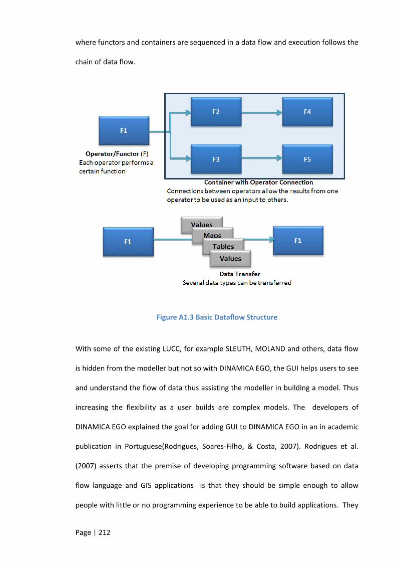
Page | 212

where functors and containers are sequenced in a data flow and execution follows the

chain of data flow.

Figure A1.3 Basic Dataflow Structure

With some of the existing LUCC, for example SLEUTH, MOLAND and others, data flow

is hidden from the modeller but not so with DINAMICA EGO, the GUI helps users to see

and understand the flow of data thus assisting the modeller in building a model. Thus

increasing the flexibility as a user builds are complex models. The developers of

DINAMICA EGO explained the goal for adding GUI to DINAMICA EGO in an in academic

publication in Portuguese(Rodrigues, Soares-Filho, & Costa, 2007). Rodrigues et al.

(2007) asserts that the premise of developing programming software based on data

flow language and GIS applications is that they should be simple enough to allow

people with little or no programming experience to be able to build applications. They

Page | 213

pointed out that, a major challenge to the development of such an environment is to

maintain its traditional simplicity as this tool becomes more sophisticated and the

models grow in complexity (Abran et al., 1996). This is the point where there is a need

for a powerful and user-friendly interface that allows the user, whether beginner or

advanced, to implement models of cartographic algebra quickly and / or intuitively.

Therefore, the nature of Dinamica EGO graphical user interface (GUI) was based on the

theory of directed graphs, in which information starts from a point, follows a path

guided by the connections of nodes in the graph (functors) and arrives at another point

in the graph, not necessarily different from the original. Thus, by means of the arrows

the functors are connected through its input and output ports, according to the

processing order desired (Rodrigues et al., 2007).

Figure A1.4 Functor Port Editor of Determine Transition Matrix

Port Editor

Each port editor has input and out

port for input and out data

respectively. The Determine

Transition Functor Port Editor takes

in two data, that are initial map

and final map. Time steps port can

edited with discrete time step.

Outputs are tables/matrices.

Page | 214

The “Dinamica” data flow language describes the thread and the relationship between

the operators. The benefit of this internal representation is to simplify the analysis of

the time needed for a result to be kept in memory since the dependencies between

the operators can be obtained quite trivially, even when the dependencies involve

containers with an arbitrary level of nesting. Thus Dinamica balances computational

resource use rationally, utilising little memory even in very complex models. Moreover,

the analysis of the dependencies assists in calculating the execution order of the

operators. This approach differs from the traditional approach that uses a table to

determine when an operator can run(Johnson, Hanna, & Millar, 2004). The previous

calculation of the execution order allows operators to be grouped so that an operator

runs close to that which uses its result, thus avoiding a large data structure, such as a

map, being retained in the memory longer than necessary. This calculation is also

compatible with the conditional execution of functors, allowing operators that perform

one or more functors/containers based on an intermediate result to be easily

defined.(Rodrigues et al., 2007)

The models created by combining these operators are written in the form of textual

scripts. Scripts can be created in two different formats, XML Script or EGO.

Most of Dinamica operators execute its internal operations in parallel and take

advantage of execution environments with multiple processors or cores, for example,

dividing the task applied on a given map between multiple processors(Rodrigues et al.,

2007), thus the Auckland Region LUCC model implemented in DINAMICA with input

data 1251x1531 pixels executes faster (about 100 times) compared to SLEUTH. For

comparison, a model implemented in Dinamica EGO that calculates the lowest cost

route on a map with 900x900 cells is sixty times faster than the same model

Page | 215

implemented on the MacroModeler Idrisi (Eastman, 2003). With regard to the

computational model performance, another great advantage is that while other

modelling environments in GIS (e.g. MacroModeler and the Idrisi ModelBuilder of

ArcGIS) use modules that write their results in the disk to be read again at a later step,

thereby penalizing its performance, Dinamica uses a continuous flow of data that is

held in memory only as needed to run the model.

DINAMICA EGO is not an actual model like SLEUTH, LEAM and or MOLAND but a

modelling software environment with the requisite tools for environmental modelling.

Thus this makes it open for modellers to build their own models from start to finish,

also existing models can be rebuilt in DINAMICA EGO. The most commonly used

operators (functors) by environmental modellers are predefined and there is the

option for user defined operator (functors), this capability of DINAMICA gives users the

degree of freedom for selecting operations and techniques to use. For example a user

can choose to use weights of evidence of coefficients in calibrating or use the Genetic

Algorithm approach or custom made functor for calibration.

DINAMICA EGO was found to be more suitable for this research because of its

architectural environment and functions. That is:

DINAMICA EGO uses CA transition function as the engine for simulation

models, such as LUCC, and the modelling technique adopted for this research is

CA.

DINAMICA EGO is not a model but modelling software environment therefore

gives modellers degree of freedom to test many variable as possible through

the functors. Unlike other models with fixed variables and modellers can only

Page | 216

change the coefficients and not the variables. Therefore modellers cannot test

the significance of the variable before including in the model, but this can be

done in DINAMICA.

It is simple and easy to use through the GUI. There is no programming skill

needed, just drag and drop the functors whilst with SLEUTH some programming

skill is need in creating “scenario” files.

Its flexibility increases as model becomes complex. This research is to

investigate ten LUCC transitions and which is complex to build.

Its performance is high due to optimization of speed and computation

resources such as use of memory and parallel processing. This favours the huge

data size (1251x1531 cells) per map or input data and ten (10) LUCC transition

of this work.

Geospatial Process Modelling for Land Use Cover Change

Documents

Transcript of Geospatial Process Modelling for Land Use Cover Change