1

Water drainage in double-porosity soils: experiments and micro-macro modelling.

Jolanta Lewandowska 1, Tien Dung Tran Ngoc 2, Michel Vauclin 3 and Henri Bertin 4

Abstract: This paper presents the experimental validation of a macroscopic model of

unsaturated flow in double-porosity soils, which was developed using the asymptotic

homogenization method. The model was implemented into a code which enables micro-macro

coupled calculations of macroscopically one-dimensional and microscopically three-dimensional

problems. A series of drainage experiments were carried out in a column filled with a double

porosity medium. The porous medium is composed of Hostun sand and porous spheres made of

sintered clay, periodically distributed in the sand. The characteristic pores sizes of the two media

differ by two orders of magnitude. During the experiments the water content evolution inside the

column, the capillary pressure and the flux at the bottom of the column, were measured. The

numerical simulations results showed a good agreement with the experimental data, confirming

the predictive ability of the model. The experimental and numerical evidence of the influence of

the micro-porous inclusions on the flow dynamics (flux retardation, water retention in the micro-

porosity), is clearly shown.

CE Database subject headings: Unsaturated soils, nonuniform flow, drainage, microstructure, heterogeneity, scale effect, gamma rays, model verification. Submitted to the Journal of Geotechnical and Geoenvironmental Engineering, October 2006 Revised version May 8th, 2007. Final version July 26th, 2007.

2

1 Assistant Professor, Laboratoire Sols, Solides, Structures-Risques (3S-R), UMR 5521, CNRS, UJF, INPG, BP 53, 38041 Grenoble cedex 9, France. (corresponding author). Tel: (33) 476825181. Fax: (33) 476827000. E-mail: jolanta.lewandowska@hmg.inpg.fr 2 Ph. D. Student, Laboratoire d’étude des Transferts en Hydrologie et Environnement (LTHE), UMR 5564, CNRS, UJF, INPG, IRD, BP 53, Grenoble cedex 09, France. 3 Directeur de Recherche, Laboratoire d’étude des Transferts en Hydrologie et Environnement (LTHE), UMR 5564, CNRS, UJF, INPG, IRD, BP 53, Grenoble cedex 09, France.

4 Directeur de Recherche, Laboratoire TRansferts, Ecoulements, FLuides, Energétiques (TREFLE), UMR CNRS 8508, Université de Bordeaux, 33405 Talence cedex, France.

3

Introduction

Modelling of unsaturated water flow in soils is still a problem of great interest because of

geotechnical and geoenvironmental applications, such as construction of earth dams and dikes,

protection of groundwater resources from chemical pollution or securing waste landfill. The

recent advances concern two main difficulties related to this topic: the heterogeneity of the soils

and the non linearity of the involved processes. Both features are at the origin of the

development of macroscopic models which are able, on one hand, to take into account the

microstructure of soils and their influence on the water flow dynamics, and on the other hand, to

simplify the mathematical description in order to make it tractable from numerical point of view.

Natural soils are complex heterogeneous structures. A particular class of heterogeneous

soils, which are characterized by the existence of two distinct sub-regions with highly contrasted

hydraulic properties, can be named double-porosity media. In this case, one of the sub-domains

is associated with high hydraulic conductivity (inter-aggregates, fractures or fissures) and

another one with low conductivity (aggregates, porous matrix). In practice it is difficult (even

impossible) to represent the heterogeneous microstructure of such soils, therefore macroscopic

models which replace these porous media by equivalent homogeneous continuum, have to be

considered.

Modelling water flow in unsaturated double-porosity soils was the subject of much

research in the scientific literature. Different approaches were adopted in order to address the

question of non-standard behaviours of this soil type, which can not be described by the classic

single-porosity model (Richards 1931). The phenomenological models were recently reviewed

by Šimůnek et al. (2003). These models are based on the concept of two overlapping sub-

regions, initially proposed by Barenblatt et al. (1960). Generally, models of this type are called

4

two-regions/two-equations models, because every region is represented by an equation according

to the different conceptualizations and an exchange term links the two equations. When water

flow is assumed to occur only in the macro-region (inter-aggregates, fractures or fissures) and is

stagnant in the micro-region (intra-aggregates, porous matrix), we have the dual-porosity model

or mobile-immobile model (MIM) (van Genuchten and Wierenga 1976). In this model the

immobile region is responsible for the water exchange, which is defined by the difference of the

effective water saturations and a first-order rate coefficient. The dual-porosity model is

considered as the “classic dual-porosity model” by Brouyère (2006). Since the assumption of

uniform water content in the micro-porosity is questionable from the physical point of view

(Zurmuhl and Durner 1996), an adjustment of the dual-porosity model called “dynamic dual-

porosity model” was recently proposed by Brouyère (2006). Gerke and van Genuchten (1993a,

1993b) developed the dual-permeability model, in which the Richards equation is written for

each sub-domain and the mass transfer term is assumed to be proportional to the pressure head

difference between the two sub-domains. This means that water flow occurs not only in the

macropores, but also in the micropores. This approach requires the knowledge of water retention

and hydraulic conductivity functions for both porous regions, as well as the hydraulic

conductivity function of the fracture-matrix interface (Šimůnek et al. 2003). The expressions of

the exchange term for the two-region models were also proposed by Barker (1985), Dykhuizen

(1990) and Zimmerman et al. (1993). The verification of the dual-porosity/permeability model

was carried out for example by performing a series of upward infiltration experiments on

undisturbed soil column (Šimůnek et al. 2001). Although these models were able to reproduce

the non-equilibrium behaviour in a particular case, the general definition of the range of their

validity was not given. Therefore, they can not directly be applied to other situations (other

5

materials, other flow conditions). The dual-permeability models were also developed for

fractured rock and their complete overview can be found in Doughty (1999) and Doughty and

Karasaki (2004). Another type of description is proposed in the MACRO model of Jarvis (1994).

The water flow is described by the kinematic wave equation (German and Beven 1985) in the

more conductive sub-region, whereas the Richards equation is applied in the soil matrix. The

water exchange between micro and macropores is assumed to be proportional to the saturations

difference.

An alternative approach with respect to the phenomenological models cited above is the

up-scaling by applying the homogenization methods. Quintard and Whitaker (1988, 1990) used

the volume average method to derive a macroscopic model for two-phase flow in heterogeneous

media. This model was validated by experiments performed on two different types of nodular

media (continuous sand matrix with sandstone inclusions and sandstone matrix with sand

inclusions) (Bertin et al. 1993). Another type of up-scaling is the asymptotic homogenization

method. By applying this method, Arbogast et al. (1990) and Douglas et al. (1997) proposed

models of single-phase flow in double-porosity media. Showalter and Su (2002) developed a

model of partially saturated flow in a composite poroelastic medium. Lewandowska et al. (2004)

presented a model of transient flow in unsaturated double-porosity soil. The resulting model was

successfully verified by performing a series of numerical tests of water infiltration, the results of

which were close to the fine-scale reference solutions. The formal mathematical proof of

existence and uniqueness of the solution of this double-porosity model was presented by Mikelic

and Rosier (2004). A good agreement between the model and experimental data of infiltration

tests performed in a double-porosity soil was reported by Lewandowska et al. (2005). However,

these data were limited to the cumulative fluxes at the inlet and the outlet to the column. Since

6

they can result from various conditions inside the column, they are not sufficient for definitive

validation of the model. What is needed is the information on the water content and capillary

pressure (the unknowns of the problem) inside the column. Also, the fact that hysteresis is

neglected in the model makes it necessary to validate the model in other flow conditions like

drainage, in which the response of the double-porosity medium can be different.

The aim of the present paper is the experimental validation of the double-porosity model

(Lewandowska et al. 2004) in the case of water drainage, including the measurements of water

content and capillary pressure inside the column during the flow. A series of one-dimensional

experiments were carried out in a column filled with a porous medium composed of sand and

sintered clayey spheres embedded in a periodic manner. The experimental results are compared

with the double-porosity model, which was implemented into a code (Szymkiewicz and

Lewandowska 2006), enabling the micro-macro coupled calculations of unsaturated water flow.

Experiments

Experimental strategy

The experimental strategy consisted of performing the same type of drainage tests in two

materials, namely: homogeneous sand and double-porosity medium (sand with porous inclusions

of spheres made of sintered clay). The aim of this strategy was twofold. First, compare the

behavior of these two porous media, in order to investigate the influence of the double structure.

Second, once the individual hydraulic parameters of the two components (sand and sintered

clay), were known, apply the homogenization technique developed in Lewandowska et al. (2004)

in order to predict the behavior of the double-porosity medium and compare it with experimental

observations. Each test was repeated twice. The hydraulic parameters of sand were determined

7

by an inverse analysis based on the results of one of the drainage tests (Test 1). The other

drainage test (Test 2) was used as a validation of these parameters by performing direct

calculations. Concerning the sintered clay material, previous results obtained in the case of

infiltration (Lewandowska et al. 2005) were used, since we were not able to perform drainage

experiments in this material. The clay being of low permeability (high air-entry pressure), a

gravity drainage on a short core (available) was not possible. Finally, the two experiments

performed in the double-porosity medium were interpreted individually and experimental data

compared with the double-porosity model simulation.

Experimental set-up

The experimental set up consisted of a column, equipped with a tube at its bottom,

allowing the application of a negative pressure. The inner diameter of the column was 6 cm and

its total height was 60 cm. The column was installed in a rig (Fig. 1) moving the gamma rays

attenuation device (Lewandowska et al. 2006). The following quantities were measured during

the experiments: the volumetric water content (θ), the capillary pressure (h) and the cumulative

mass of water drained out of the column (F). The water content was measured by the gamma

rays attenuation technique (Corey et al. 1970; Gharbi et al. 2004) that is based on the selective

attenuation of the solid and fluid phases. The mass of water drained from the column was

measured by a balance. The data were registered every 5 s and transferred to a computer via a

datalogger (Campbell Scientific Ltd CR 10 X).

The experimental protocol consisted of four principal stages. First, the porous medium

was packed in the column. Each layer of the medium was mechanically compacted and its

porosity was controlled. Then, the column was filled up with several pore volumes of CO2 in

8

order to drive out the air and attain full initial water saturation. After that water was allowed to

infiltrate into the column from the bottom and to push out CO2. The principal step of the

experiment started after the water saturation was reached. It consisted of the drainage of water at

a constant capillary pressure (∆h) imposed at the bottom of the column.

Drainage experiments in sand

In the experiments we used the Hostun sand HN38 that is a fine calibrated quartz sand (Flavigny

et al. 1990). The grain distribution of the sand was relatively uniform with the mean grain

diameter of 162 µm (Lewandowska et al. 2005). The sand was compacted. Two drainage

experiments (Test 1 and Test 2) were performed. In each case the capillary pressure applied at

the bottom was the same and equal to - 0.85 m, Tab. 2.

It was assumed that the sand hydraulic properties were adequately described by the van

Genuchten-Mualem (Mualem 1976, van Genuchten 1980) equations:

( ) ( ) ( )[ ] mnRSR hh

−+−+= αθθθθ 1 (1)

for the water retention curve, and:

[ ] 2/21 )(1)(1)(1)(

mnmnnS hhhKhK

−−− +

+−= ααα (2)

for the unsaturated hydraulic conductivity. θR and θS [-] are the residual and saturated volumetric

water content, respectively, KS is the hydraulic conductivity at saturation [LT -1], α [L -1] , n [-]

and m [-], (with m = 1-1/n) are empirical constants.

The retention curve h(θ) was measured directly at the end of the drainage experiments,

once the hydrostatic equilibrium was reached. Then, an inverse procedure using the HYDRUS-

1D code (Šimůnek et al. 1998) was used to determine the parameters of Eqs (1) and (2). To

9

overcome the non uniqueness problem, the number of fitting parameters was reduced to two (α

and n), since the three others (θS, θR and KS) were determined from other experiments

(Lewandowska et al. 2006). In the inverse analysis the h(θ) data, as well as the water content

versus time θ(t) at fixed depths z and the cumulative water flux at the bottom of the column F(t )

from Test 1, were used. The total number of input data (of equal weight) was equal to 129: 33

data points for h(θ), 15 data points for θ(t) and 81 data points for F(t). The resulting adjusted

parameters are: α = 9.31× 10-1 m-1 and n = 8.567, while the values of the remaining (fixed)

parameters are: θS = 0.399 m3/m3, θR = 0.022 m3/m3 and KS = 2.86 × 10-5 m/s, Tab. 1. In Fig. 2

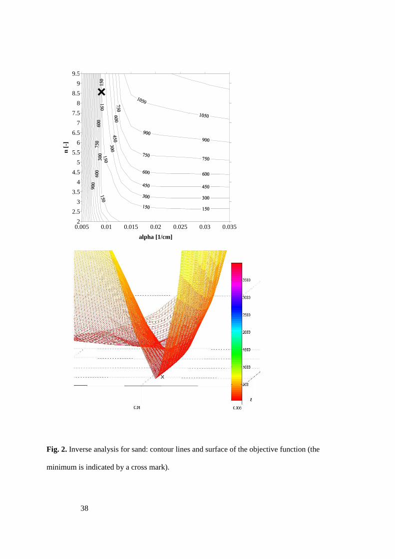
the isolines of the objective function as a function of the parameters α and n are plotted. The

objective function is of valley-type. The bottom of the valley is slightly tilted. This behavior is

often reported in the literature, and is associated with the correlation of the parameters. The

minimum point is marked by a cross. As it can be seen it is not well defined. However, since we

investigated a large spectrum of parameters and we repeated the search for various initial values

it can be assumed that this fitting is the best that can be obtained using the van Genuchten–

Mualem model. The water retention θ(h) and the hydraulic conductivity K(h) curves of the

Hostun sand are presented in Fig. 3.

The obtained hydrodynamic functions were used to perform the direct calculations of

drainage in the Hostun sand for Test 2. The comparison between the calculated and measured

cumulative and instantaneous water fluxes at the bottom of the column is presented in Fig. 4 (the

experimental results for Test 1 are also shown). A good agreement can be observed at the

beginning of the drainage process while, after about 5000 s the calculated cumulative flux

diverges slightly from the experimental values (Fig. 4 a). Moreover, the characteristic time of the

phenomenon is not precisely reproduced, since we observed an abrupt interruption of flow, while

10

the model predicts a continuous but very slow increase of the cumulative water flux. The

experimental behavior suggests that the threshold - type hydraulic functions should be used.

However, we were limited by the inverse analysis proposed by commercial codes and the

implemented van Genuchten-Mualem model, since the inverse analysis is a problem itself,

beyond the scope of the paper.

The calculated and measured water content are compared in Figs. 5, 6 and 7. The

comparison requires a comment. Measurement of the water content using the gamma rays

attenuation technique is not instantaneous. It takes about 5000 s to perform 33 measurements

along the column. Each value of the calculated water content profile corresponds to a position in

the column and a time of measurement at that point. It means that the whole profile can not be

treated as an instantaneous picture of the distribution of the water content in the column at time t.

In Fig. 5 a good agreement between the calculated and measured initial and final water content

profiles, can be seen. In Fig. 6 the profiles of the water content variations between the initial

saturated value and the transient value ∆θ = θS – θ(t), are plotted. The observed scatterings can be

explained by the difficulties of measuring a transient process. Another kind of interpretation of

the same data is shown in Fig. 7 where the measured evolution of the water content at three

positions in the column is compared with the calculated values. A good agreement is observed

for the first and the second point of measurements, and worse for the third. This trend is seen in

both tests. These tests differ in the direction of measurement (Test 1: from the top to the bottom;

Test 2 : from the bottom to the top). This fact indicates the accumulation of errors due to the non

instantaneous measurement.

11

Drainage experiments in the double-porosity medium

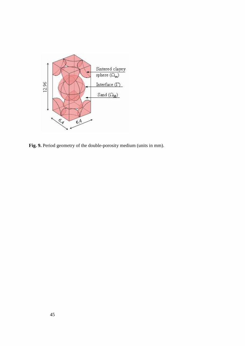
The double-porosity medium used in the experiments was a periodic arrangement of spheres

(mean diameter of 6.4 mm) made of sintered clayey material, embedded in the Hostun sand

HN38. The clayey spheres were homogeneous without a skin effect due to reduced porosity (Fig.

8). The pore size distribution was very narrow, with a mean pore of 0.7 µm (Lewandowska et al.

2005). The total porosity of the sintered clay material obtained from the mercury porosimetry

was φm = 0.376. The skeleton specific density was ρs = 3001 kg/m3 and its dry bulk density ρd =

1880 kg/m3. The column was gradually and carefully filled with sand and spheres layer after

layer. The mass of each layer and the energy of compaction were controlled. The obtained

periodic microstructure of the double-porosity medium is presented in Fig. 9. For the spheres the

parameters previously obtained from infiltration tests (Lewandowska et al. 2005) were used. It

was assumed that the possible error is negligible, since it was shown that the unsaturated water

flow in double-porosity medium is primarily governed by the macroporosity (Lewandowska et

al. 2004). The hydraulic parameters of the van Genuchten-Mualem model for the sintered clay

are reported in Table 1.

Two experiments of drainage of the double-porosity medium (Test 3 and Test 4) at

constant capillary pressure head (–0.85 m) imposed at the base of the column, were performed.

Their main characteristics are given in Table 2. The same experimental protocol as for the sand

column was followed. The experiments took longer time than in sand, because of the presence of

microporosity. Thanks to the gamma ray attenuation technique, the saturation of the double

porosity medium was well controlled. It was achieved after about 32 h, against 14 h in sand for

the same pumped water rate.

12

Note that for the reason of comparison the porosity of sand in the double-porosity

medium was kept the same as in the case of the experiments carried out in the homogeneous

sand. We measured the water content inside the column and the cumulative flux at the bottom of

the column during the whole experiment.

Micro-macro modeling of unsaturated water flow in the double-porosity medium

Macroscopic model

Modeling unsaturated water flow in the double-porosity medium should take into account the

contrast between the hydrodynamic parameters which comes from the double structure at the

microscopic level. Such a model can be obtained by applying the asymptotic homogenization

method (Bensoussan et al. 1978; Sanchez-Palencia 1980; Auriault 1991). It consists of two

coupled equations: one equation describing the water flow in the macro-porosity (ΩM), and one

equation concerning the local flow in the micro-porosity domain (Ωm). They are written as

follows (Lewandowska et al. 2004):

0),())()((-∂∂

)( 3 =++⋅ thQehht

hhC MMM

effMM

eff r∇∇∇∇∇∇∇∇ K (3)

0))((-∂∂

)( =⋅ mmmm

mm hht

hhC ∇∇∇∇∇∇∇∇ K in Ωm (4)

where hM and hm [L] are the capillary pressure heads in the macro- and the micro-porosity

respectively, Ceff is the effective retention capacity of the double-porosity medium, and Cm [L -1]

the retention capacity in the micro-porosity domain, Keff [LT -1] is the effective hydraulic

conductivity of the double-porosity medium and Km [LT -1] the hydraulic conductivity in the

micro-porosity domain and 3er

[L] is the unit vector oriented positively upwards. Equation (3) is

written in global coordinates, while Equation (4) is in local coordinates. The coupling term Q

13

(hM, t) in Eq. (3) corresponds to the rate of variations of the average water content in the micro-

porosity domain. It is expressed as:

td

t

hCthQ m

mm

mmM ∂

∂=Ω∫ ∂

∂Ω

=Ω

θ1),( (5)

The boundary conditions for Eq. (3) are the conditions imposed at the macroscopic boundaries,

while the boundary condition for Eq. (4) is the continuity of the capillary pressure at the macro

and micro-porosity interface Γ:

hM = hm on Γ (6)

The model includes two effective parameters Keff and Ceff which are defined as follows:

Ω+χ∫Ω=

Ωdhh M

MMM

eff ))((1

)( IKKr

∇∇∇∇ (7)

)()( 1 MMMeff hCwhC ×= (8)

where KM [LT -1] and CM [L -1] are the unsaturated hydraulic conductivity and retention capacity

of the macro-porous domain (ΩM) respectively; w1 is the volumetric fraction of ΩM in the period

Ω; I is the identity matrix. The vector function χr is a solution of the local boundary value

problem (or closure problem), resulting from the homogenization process. This problem is

defined as follows:

0))((( =+χ⋅ IKr

∇∇∇∇∇∇∇∇ MM h in ΩM (9)

with the zero-flux boundary condition on the interface Γ:

0))(( =⋅+χ NhMM

rrIK ∇∇∇∇ (10)

where Nr

is the unit vector normal to Γ, and the periodicity on the external boundaries of the

period and the zero-volume average condition. For more details the reader can refer to

Lewandowska et al. (2004).

14

Numerical solution

The double-porosity model described by Equations (3) - (5) requires a particular strategy of

numerical solution since both equations are highly non-linear and coupled. The simultaneous

solution in the macro and micro-domains was previously proposed in the literature for other

problems (see for example: Pruess and Narasihman 1982; Huyakorn et al. 1983). In the case of

experiments reported in the paper, both problems (macroscopic and microscopic) are one-

dimensional. The problem was solved using the two scale finite difference method

(Lewandowska et al. 2004, Szymkiewicz and Lewandowska 2006). First, the macroscopic

domain was discretized. Then, each macroscopic node was associated with a local-scale

numerical grid, representing the inclusion. The calculations were performed simultaneously at

these two scale levels, with the transfer of information at each time step. The main characteristics

of the numerical solution are the following: the mixed (θ-h) formulation of the flow equations,

the implicit scheme of time integration, the Newton method for solving the non linear equations,

and time step adjusted automatically to meet the accuracy and stability requirements. The initial

and boundary conditions were:

- for t ≤ 0 : h = 0 within the whole domain (saturation).

- at z = 0 and for t > 0: Keff (∂h/∂z + 1) = 0 (zero flux at the top of the column).

- at z = -L and for t > 0, h = - 0.85 m of water.

3.3. Effective hydraulic parameters of the double-porosity medium

In order to calculate the effective conductivity tensor, the local boundary value problem (Eqs 9

and 10) in the period domain (Fig. 9) was solved, using the commercial code COMSOL

15

Multiphysics. In our particular case, only the χ3 component was needed, since we were interested

in the vertical component K33 of the conductivity tensor. According to the expressions (7) and

(8), the effective conductivity and effective capillary retention capacity of the double-porosity

medium are respectively:

)(330.0)( hKhK Meff ×= (11)

and

)(483.0)( hChC Meff ×= (12)

where )(hKM and )(hCM are the corresponding hydraulic properties of sand.

Comparison between numerical results and measurements for the double-porosity

medium.

The experimental data of Test 3 and Test 4 are compared with the numerical solution of the

unsaturated water flow equation in the double-porosity medium.

The cumulative flux is one of the criteria of comparison of the results presented in our

paper. The other ones are: the distribution of the water content and the evolution of the capillary

pressure in the column during the process. We believe that the data concerning the water content

and the capillary pressure distribution (and their time evolution), are more pertinent for

comparisons than the cumulative flux. The reason is twofold: i) the water content and the

capillary pressure are unknowns, and are direct solutions of the boundary value problem, while

the cumulative flux at the boundary follows from the post treatment. ii) as a measured quantity

the cumulative flux integrates all the errors in the domain and in time, therefore it appears less

reliable than data inside of the domain.

16

Cumulative and instantaneous water fluxes

The time evolutions of the cumulative and instantaneous water fluxes at the bottom of the

column are presented in Fig. 10. It can be seen that the total amount of drained water measured at

the end of the experiments (4.95 × 10-2 m) differs from the calculated one (5.52 × 10-2 m) by

about 10% which is considered to be acceptable. Another element of comparison is the

characteristic time of the process. The model does not fit it correctly, as in the case of sand.

While the measured values indicate that the water apparently ceased to flow out of the column at

t ≈ 10000 s, the calculated cumulative flux continues to increase slightly with time. This can be

explained by means of the same arguments as was discussed in case of the sand. On the other

hand, the transient simulated and observed cumulative fluxes are in good agreement. Also, the

instantaneous water flux is fairly well described; the scatterings could be related to the precision

of measurement (0.7 × 10-5 m/s).

Water content distribution

The calculated initial and final water content profiles are compared with the experimental

observations in Fig. 11. The calculated water content is an average value of the water content in

the micro and macro-porosity domains, taking into account the volumetric fraction of each

domain. It clearly appears that the measurements are much more scattered than in the case of

sand (Fig. 5). This is due to two main reasons: i) the presence of heterogeneities of periodic

structure and characteristic size of 12.96 mm (Fig. 9), and ii) the size of the gamma rays

collimated beam (5 mm) that provides an “average” measured value. It can be noticed that the

measuring technique is not well adapted to the experience. Nevertheless, relatively good

agreement in terms of average values can be observed.

17

Fig. 12 shows the water content profiles variations, i.e., the difference between the initial

and current state of water content during the transient phase of flow. It can be seen that the

observations are scattered around the simulation line. The negative values observed at the bottom

of the column in the first profiles give us information about the order of magnitude of the total

measurement precision, which is about 3% (in water content). We can also argue about the

capacity of the outlet of the column to evacuate water instantaneously. In Figure 13 the measured

time evolution of the water content at three positions in the column is compared with the

calculated values. Fig. 13 a deals with Test 3 in which the measurements started at the top of the

column, while Fig. 13 b presents Test 4 in which the measurements started at the bottom. A good

agreement is observed in both cases at two of three positions in the column, showing the

influence of the measurement protocol (see discussion for sand).

In order to quantify the performance of the model all results dealing with the water

content (prediction versus observation) are collected in Fig. 14. We chose arbitrarily a band of ±

0.05 as a limit value of prediction precision. The four water content profiles, corresponding to

different times, are characterized by the following percentage of results lying within the

precision band: 80%, 70%, 64% and 64%. The decreasing order means that the quality of the

prediction of the water content decreases with time. However, one has to take into account that

the initial state at saturation is characterized by 80%, which means the initial dispersion of the

water content measurements. Therefore, we believe that in the transient phase the model works

relatively well. Another way to evaluate the model performance consists in calculating the

following indicators (Tedeschi et al. 2006):

- Mean bias, N

POMB

N

iii∑ −

= =1)( (13)

18

- Mean relative error, ∑

−=

=

N

i i

ii

O

PO

NMRE

1

100 (14)

- Root mean square error, N

OPRMSE

N

iii∑ −

×= =1

2)(100 (15)

- The range of variation of the observed and predicted values of the water content for each

profile, RV = (min Oi, max Oi) and (min Pi, max Pi) (16)

where Oi and Pi are the ith observed and predicted value of the water content, respectively; N is

the number of measurements.

The calculated values of the statistical indicators MB, MRE, RMSE and RV for each

profile of the water content are given in Table 3. The analysis of the indicators shows that the

model in average underestimates the water content (MB > 0), or in the other words, it

overestimates the time variations of the water content. It can be seen that the values of MB

indicator are of the same order of magnitude that the estimated precision of the water content

measurements by the gamma attenuation technique (3%). The maximum value of the mean

relative error (MRE) occurs at the end of drainage (14.7% and 18.1%). The root mean square

error (RMSE) varies between 3.9 % and 6.2 %. The range of variation of the water content is

higher for the observed values (due to scatterings) than the calculated one. In conclusion, the

analysis of the statistical indicators confirms that the model gives relatively good results with a

slight underestimation of water content (or overestimation of the variations of water content).

This is also reflected in the fact that the total calculated cumulative flux drained from the column

is greater than the measured one.

The double-porosity effect

19

The presence of the micro-porous inclusions is responsible for the drainage retardation in the

double-porosity medium with respect to the homogeneous case (sand). For instance, while 86

mm of water (cumulative flux) was recovered at the outlet of the sand column at the end of

drainage (Fig. 4 a), only 48 mm was measured for the double-porosity medium (Fig. 10 a) at the

same time. Another feature of the observed double-porosity effect is the retention of water in the

micro-porosity that can be seen by comparison of the total water volume drained from the sand

(Fig. 4 a) and the double-porosity column (10 a) after the completion of drainage in both media.

The volume difference represents the water retained in the micro-porosity domain (porous

spheres).

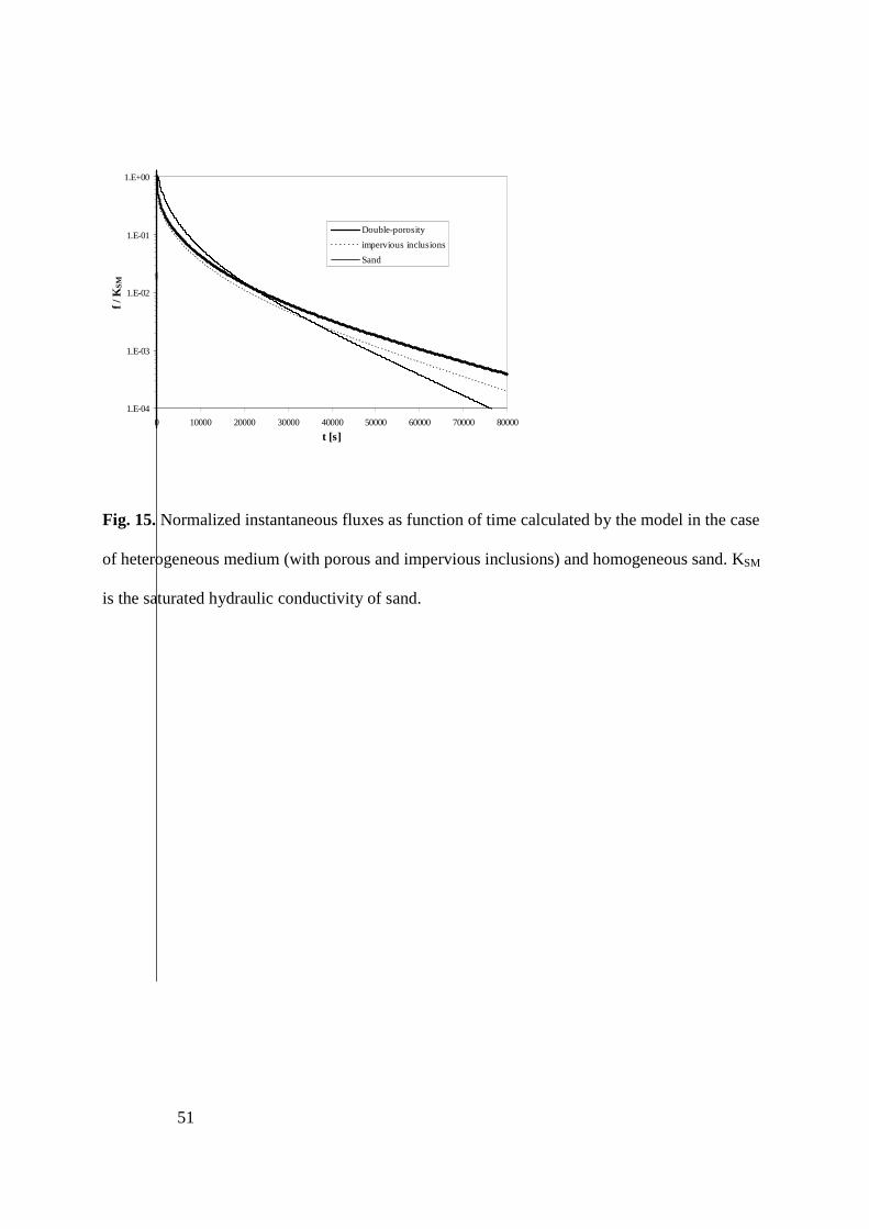
The double-porosity effect can also be observed from the results of calculations. In Fig.

15 the instantaneous fluxes in the sand and the double-porosity medium (normalized by the

saturated hydraulic conductivity of sand, KSM), are plotted versus time. In order to separate the

different contributions, the case of totally impervious inclusions is also presented. In this case all

the other parameters, like volumetric fraction and arrangement of spheres are the same. First, it

can be seen that the flux in the sand is slightly higher than the flux in the double-porosity

medium until t = 22000 s. Then, this trend is reversed and the flux in sand decreases

dramatically, while it persists over long time in the double-porosity medium. For instance, at t =

75000 s, the two fluxes differ by about one order of magnitude. Secondly, it can be noticed that

the flux corresponding to the case of impervious inclusions lies between the two other fluxes.

The comparison of these three fluxes shows : i) the influence of spherical obstacles, if we

compare the behavior of homogeneous sand with the sand containing impervious spheres, and ii)

the effect due to the micro-porosity domain, when the behavior of sand with porous and with

impervious inclusions (spheres), are compared.

20

Domain of validity

The domain of validity of the double-porosity model is defined as a function of the ratio of the

diffusivity coefficients of the micro (Dm) and macro porosity (DM) domains (Lewandowska et al.

2004):

Dm / DM = O(ε2) or Dm / DM << O(ε1) (17)

where the water diffusivity coefficient is the ratio of the hydraulic conductivity over the capillary

retention capacity, D = K/C and ε is the scale separation parameter. It is defined as: ε = ℓ / L,

where ℓ is the characteristic microscopic length (dimension of the period) and L is the dimension

of the macroscopic domain (length of the column). In our case we have: ℓ = 12.96 × 10-3 m, L =

0.5 m, and consequently ε = 2.6 × 10-2. It can be concluded that the model is valid when Dm / DM

<< O(10-2), which means of the order O(10-3) or less. The ratios of the hydraulic parameters of

the micro-porous domain over those of the macro-porous one, as a function of capillary pressure,

are plotted in Fig. 16. It can be seen that the condition of validity of the model was satisfied as

long as |h| remained smaller than about 0.6 m of water (the “wet” domain). That corresponds to

the early stages of the drainage when the porous medium is still wet. It is not verified for higher

values of the capillary pressure, i.e. at the upper part of the column at longer time. However, the

experimental data presented in this paper were also interpreted using a generalized unsaturated

flow model for heterogeneous media which is valid for all ratios of the hydraulic diffusivities

(Szymkiewicz and Lewandowska 2006). The results (not presented here) were found to be very

close to the double-porosity model, which means that in this case the flow is somehow

dominated by the “wet regime”.

21

Conclusions

The double-porosity unsaturated flow model obtained by upscaling using the asymptotic

homogenization method, was presented. It has been evaluated against a series of laboratory

drainage experiments. A good general agreement between numerical simulations and

experimental observations illustrates the predictive capacity of the model. Of particular interest

was the influence of the micro-porous inclusions on the dynamics of flow, as compared to the

homogeneous medium. The effects are flux retardation and water retention in the micro-porosity.

Difficulties were encountered in the interpretation of the measurements performed in the

double-porosity medium. First, the medium was highly heterogeneous and the size of the

heterogeneity was obviously finite. From the point of view of the applicability of the continuous

description, the dimensions of heterogeneity should tend to zero. In the experiments they were

kept as small as possible to obtain an acceptable scale separation. The scale separation, defined

as the ratio of the height of the period over the length of the column, was of the order 1:100

which is often considered as a limit value. Second difficulty dealt with the choice of the

measuring technique of the water content, which should be appropriate for transient flow in

heterogeneous medium. The question of what was really measured (what kind of time and space

average?), which is an important issue in all experiments, appears fundamental in the case of

laboratory experiments in highly heterogeneous media. Therefore, even though we tried to

respect all the constraints to a maximum extend, the results carry the errors related to the issues

quoted above. Moreover, the statistical treatment of the experimental data turned out to be

delicate because of the relatively small number of data and the high non linearity of the model.

For all these reasons the question concerning the model performance can not be addressed in a

more detailed manner than presented in the paper.

22

Finally, the results clearly showed qualitative and quantitative differences in the flow

dynamics occurring in the homogeneous and heterogeneous medium. This behaviour may have

consequences not only for the water flow predictions but also for related aspects such as solute

transfer and hydro-mechanical phenomena occurring in the unsaturated heterogeneous soils and

geomaterials.

The results presented in this paper can provide validation data sets for others double porosity

models. They are available upon request sent to the following address:

Jolanta.Lewandowska@hmg.inpg.fr

Acknowledgements

This research was financially supported by the project ECCO-PNRH, INSU/CNRS France (now

the GDR "Hydrodynamique et Transferts dans les Hydrosystèmes Souterrains"). We

acknowledge CNRS for the BDI-PED doctoral fellowship granted to T.D. Tran Ngoc.

Notation

The following symbols are used in this paper:

Latin letters

C = capillary capacity;

Ceff = effective capillary capacity;

CM , Cm = macro-porosity (sand) and micro-porosity (sintered clay) capillary capacity;

D = diffusivity;

DM, Dm = macro and micro-porosity diffusivities;

23

er

= unit vector;

F = cumulative flux;

f = instantaneous flux;

h = pressure head;

hM, hm = macroscopic and microscopic pressure heads;

I = identity matrix;

L = medium length;

ℓ = period size;

Keff = effective hydraulic conductivity tensor;

KM, Km = conductivity tensors in the macro and micro - porosity domain;

KS = hydraulic conductivity at saturation;

KSM = hydraulic conductivity at saturation of sand;

MRE = mean relative error;

MB = mean bias;

m = water retention function parameter;

N = number of measurements;

Nr

= unit vector normal to the interface Γ;

n = water retention function parameter;

Oi = ith observed value;

Pi = ith predicted value;

Q = water exchange between the macro and micro-porosity domain;

RMSE = root mean square error;

RV = range of water content variation;

24

t = time;

w1, w2 = volumetric fraction of the macro and micro-porosity domain;

z = macroscopic space coordinate;

Greek letters

α = water retention function parameter;

Γ = interface between the macro and micro-porosity domain;

∆h = suction imposed;

ε = scale separation parameter;

φ = mean porosity of the double-porosity medium;

φM, φm = porosity of sand (macro-porosity) and spheres (micro-porosity);

ρd = bulk density of sintered clay material;

ρs = skeletal density of sintered clay material;

θ = volumetric water content;

θM, θm = volumetric water content in the macro and micro-porosity domain;

θR = residual volumetric water content;

θS = saturated volumetric water content;

χr = vectorial function;

Ω = period domain;

ΩM, Ωm = macro and micro-porosity domain.

25

References

Arbogast, T., Douglas, J., and Hornung, U. (1990). “Derivation of the double-porosity model of

single phase flow via homogenization theory.” SIAM J. Math. Anal., 21: 823-836.

Auriault, J.L. (1991). “Heterogeneous medium. Is an equivalent macroscopic description

possible?” Int. J. Engng Sci., 29: 785-795.

Barenblatt, G. I., Zheltov, I. P., and Kochina, I. N. (1960). “Basic concepts in the theory of

seepage of homogeneous liquids in the fissured rocks.” J. Appl. Math., 24 (5): 1286-1303.

Barker, J.A. (1985). “Block-geometry functions characterizing transport in densely fissured

media.” J. Hydrol., 77: 263-279.

Bensoussan, A., Lions, J.L., and Papanicolaou, G. (1978). “Asymptotic analysis for periodic

structures.”, North-Holland.

Bertin, H., Alhanai, W., Ahmadi, A., and Quintard, M. (1993). “Two-phase flow in

heterogeneous nodular porous media” . In P. Worthington & C. Chardaire-Remière, (Eds), Adv.

in core evaluation, III: 387-409.

Brouyère, S. (2006). “Modelling the migration of contaminants through variably saturated dual-

porosity, dual-permeability chalk.” J. Contam. Hydrol., 82(3-4): 195-219.

26

Corey, J.C., Peterson, S.F., and Wakat, M.A. (1970). “Measurement of attenuation of Cs and Am

gamma rays for soil density and water content determination.” Soil Sci. Soc. Amer. Proc., 35:

215-219.

Doughty, C., (1999). “Investigation of conceptual and numerical approaches for evaluating

moisture, gas, chemical, and heat transport in fractured unsaturated rock.“ J. Contam. Hydrol.,

38(1–3): 69–106.

Doughty, C. and Karasaki, K. (2004). “Modeling flow and transport in saturated fractured rock

to evaluate site characterization needs“, IAHR J. of Hydraulics, 42, extra issue: 33-44.

Douglas, J., Peszynska, M., and Showalter, R. (1997). “Single phase flow in partially fissured

media.” Transp. Porous Media, 278: 285-306.

Dykhuizen, R.C. (1990). “A new coupling term for dual-porosity models.” Water Resour. Res.,

26(2): 351-356.

Flavigny, E., Descrues, J., and Palayer, B. (1990). “Le sable d'Hostun "RF": Note technique. ”

Rev. Fr. Geotech., 53: 67-69.

Gerke, H., and van Genuchten, M. Th. (1993a). “A dual-porosity model for simulating the

preferential movement of water and solutes in structured porous media.” Water Resour. Res.,

29(4): 305-319.

27

Gerke, H., and van Genuchten, M.Th. (1993b). “Evaluation of a first-order water transfer term

for variably saturated dual-porosity flow models.” Water Resour. Res., 29(4): 1225-1238.

German, P.F., and Beven, K. (1985). “Kinematic wave approximation to infiltration into soils

with sorbing macropores.” Water Resour. Res., 19(6): 990-996.

Gharbi, D., Bertin, H., and Omari, A. (2004). “Use of gamma ray attenuation technique to study

colloids deposition in porous media.” Experiments in Fluids, 37(5): 665-672.

Huyakorn, P.S., Lester, H. and Mercer J. W., (1983). “An efficient finite element technique for

modeling transport in fractured porous media: 1. Single species transport“. Water Resour. Res.

19(3): 841-854.

Jarvis, N.J. (1994). “The MACRO model (version 3.1). Technical description and sample

simulation”, Report and dissertation 19,51 pp., Dept. Soil Sci., Swed. Univ. of Agric. Sci.,

Uppsala, Sweden.

Lewandowska, J., Szymkiewicz, A., Burzynski, K., and Vauclin, M. (2004). “Modeling of

unsaturated water flow in double - porosity soils by the homogenization approach.” Adv. in

Water Resour., 27: 283-296.

28

Lewandowska, J., Szymkiewicz, A., Gorczewska, W., and Vauclin, M. (2005). “Infiltration in a

double-porosity medium: Experiments and comparison with a theoretical model.” Water Resour.

Res., 41(2): 1-14.

Lewandowska, J., Tran Ngoc, T.D., Vauclin, M., and Bertin, H. 2006. “Modeling by

homogeneization of water drainage in double-porosity soils.” In: C. Van Cotthem, Thimus &

Tschibangu (Eds), Proc. EUROCK 2006 - Multiphysics Coupling and Long Term Behaviour in

Rock Mechanics. Taylor & Francis Group, London: 513-518.

Mikelic, A., and Rosier, C. (2004). "Modeling solute transport through unsaturated porous media

using homogenization" Computational & Applied Mathematic, 23(2-3): 195-211.

Mualem, Y. (1976). “A new model for predicting the hydraulic conductivity of unsaturated

porous media.” Water Resour. Res., 12(3): 513-522.

Pruess, K. and Narasihman, T.N. (1982). “A practical method for modeling fluid and heat flow

in fractured porous media“, Society of Petroleum Engineers J., 14-26.

Quintard, M., and Whitaker, S. (1988). “Two-phase flow in heterogeneous porous media: The

method of large scale averaging.” Transp. Porous Media, 3: 357-413.

Quintard, M., and Whitaker, S. (1990). “Two-phase flow in heterogeneous porous media I: The

influence of large spatial and temporal gradients.” Transp. Porous Media, 5: 341-379.

29

Richards, L. (1931). “Capillary conduction of liquids through porous medium.” Physics, 1: 318-

333.

Sanchez-Palencia, E. (1980). “Non-homogeneous media and vibration theory.” Vol. 127 of

Lecture Notes in Physics, Springer-Verlag, Berlin.

Showalter, R. E., and Ning Su (2002). “Partially saturated flow in a composite poroelastic

medium.” In: J.-L. Auriault et al. (Eds), Proc. Poromechanics II (Grenoble 2002). Balkema,

Lisse: 549-554.

Šimůnek, J., Šejna, M., and van Genuchten, M.Th. (1998). “HYDRUS 1D Software package for

simulating the one-dimensional movement of water heat and multiple solutes in variably

saturated media: v. 2.0.”, IGWMC, Colorado School of Mines.

Šimůnek, J., Jarvis, N.J., van Genucten, M.Th., and Gardenas, A. (2003). “Review and

comparison of models for describing non-equilibrium and preferential flow and transport in the

vadose zone”. J. Hydrol., 272: 14-35.

Šimůnek, J., Wendroth, O., Wypler, N., and van Genuchten, M.Th. (2001). “Non-equilibrium

water flow characterized by means of upward infiltration experiments.” Eur. J. Soil Sci., 52: 13-

24.

30

Szymkiewicz, A., and Lewandowska, J. (2006). “Unified macroscopic model for unsaturated

water flow in soils of bi-modal porosity.” Hydrol. Sci. J., 51(6): 1106-1124.

Tedeschi, L.O., Fox, D.G., Baker, M.J., and Kirschten, D.P. (2006). “Assessment of the

adequacy of mathematical models.” Agric. Syst., 89: 225-247.

van Genuchten, M.Th., and Wierenga, P.J. (1976). “Mass transfer studies in sorbing porous

media: I. Analytical solutions.” Soil Sci. Soc. Am. J., 40: 473-80.

van Genuchten, M.Th. (1980). “A closed- form equation for predicting the hydraulic

conductivity of unsaturated soils.” Soil Sci. Soc. Am. J., 44: 892-898.

Zimmerman, R.W., Chen, G., Hadgu, T., and Bodvarsson, G.S. (1993). “A numerical dual-

porosity model with semianalytical treatment of fracture/matrix flow.” Water Resour. Res.,

29(7): 2127-2137.

Zurmuhl, T., and Durner, W. (1996). “Modeling transient water and solute transport in biporous

soil.” Water Resour. Res., 32(4): 819-829.

31

Table captions

Table 1. Hydraulic parameters of the van Genuchten-Mualem model for the two materials.

Table 2. Main characteristics of the experiments carried out in the sand and double-porosity

media.

Table 3. Statistical indicators of the model efficiency for the calculated volumetric water

content: Mean Bias (MB), Mean Relative Error (MRE), Root Mean Square Error (RMSE) and

Range of Variation of the observed and predicted values of the water content (RV).

32

Table 1. Hydraulic parameters of the van Genuchten-Mualem model for the two materials.

Parameter θS [-] θR [-] α [m-1] n [-] KS [m.s-1]

Hostun Sand 0.399 0.022 9.31 × 10-1 8.567 2.86 × 10-5

Sintered clay 0.295 0 6.05 × 10-1 2.27 1.15 × 10-7

33

Table 2. Main characteristics of the experiments carried out in sand and double-porosity media.

Sand Double-porosity medium Characteristics

Test 1 Test 2 Test 3 Test 4

Effective length of the column, L [m] 0.502 0.501 0.503 0.504

Porosity of sand, φM 0.396 0.399 0.386 0.389

Mean porosity of the double-porosity medium, φ - by weighting - by gamma attenuation technique

0.339 0.359

0.340 0.353

Volumetric fraction of sand, w1 0.483 0.484

Volumetric fraction of sintered clay spheres, w2 0.517 0.516 Capillary pressure imposed at the bottom of the column, ∆h [m]

-0.85 -0.85 -0.85 -0.85

34

Table 3. Statistical indicators of the model efficiency for the calculated volumetric water

content: Mean Bias (MB), Mean Relative Error (MRE), Root Mean Square Error (RMSE) and

Range of Variation of the observed and predicted values of the water content (RV).

RV [-] Test Profile MB [-] MAE [%] RMSE [%]

Predicted Observed

saturation 0.015 8.9 4.4

t = 153-5049 s 0.025 9.3 4.0 (0.30-0.34) (0.29-0.37)

t = 5733-10269 s 0.008 11.7 4 .1 (0.22-0.31) (0.17-0.35) 3

t = 80000 s 0.040 18.1 6.2 (0.16-0.31) (0.17-0.35)

saturation 0.008 9.2 3.9

t = 153-5049 s 0.019 4.9 5.8 (0.23-0.32) (0.15-0.41)

t = 5733-10269 s 0.005 17.2 5.3 (0.20-0.31) (0.14-0.35) 4

t = 80000 s 0.034 14.7 5.4 (0.16-0.31) (0.13-0.37)

35

Figure captions

Fig. 1. The experimental set-up: a) complete equipment; b) gamma ray mobile platform with

the column.

Fig. 2. Inverse analysis for sand: contour lines and surface of the objective function (the

minimum is indicated by a cross mark).

Fig. 3. Hydrodynamic properties of the Hostun sand. The curves θ(h) (bold line) and K(h) (fine

line) were fitted by the van Genuchten-Mualem model using the inverse analysis.

Fig. 4. Time evolution of calculated (lines) and measured (symbols) values of cumulative (a) and

instantaneous (b) water fluxes at the bottom of the sand column.

Fig. 5. Calculated (lines) and measured (symbols) water content profiles at the initial condition

(saturation) and the end of the experiment in the sand column.

Fig. 6. Calculated (lines) and measured (symbols) profiles of the water content variations

between saturation and transient profiles: ∆θ = θS – θ(t) in the sand column: a) Test 1: t = 153 s-

5049 s; b) Test 1: t = 5733 s – 10269 s; c) Test 2: t = 2523 s – 7419 s.

Fig. 7. Calculated (lines) and measured (symbols) water content versus time at different depths

in the sand column: a) Test 1; b) Test 2.

Fig. 8. Scanning Electron Microscopy (SEM) image of the sintered clay material: a) × 10; b) ×

5000.

Fig. 9. Period geometry of the double-porosity medium (units in mm).

Fig. 10. Double-porosity medium: Time evolution of calculated (line) and measured (symbols)

cumulative values of cumulative (a) and instantaneous (b) water fluxes at the bottom of the

column.

36

Fig. 11. Double-porosity medium: calculated (line) and measured (symbols) volumetric water

content profiles: a) initial; b) final.

Fig. 12. Double-porosity medium: calculated (lines) and measured (symbols) profiles of water

content variations between saturation and transient profiles: ∆θ = θS – θ(t) : a) Test 3 : t = 153 s –

5049 s and t = 5733 s – 10269 s; b) Test 4: t = 153 s – 5049 s and t = 5733 s – 10269 s.

Fig. 13. Double-porosity medium: calculated (lines) and measured (symbols) water content

versus time at different depths: a) Test 3; b) Test 4.

Fig. 14. Double-porosity medium: quantitative comparison between the observed and predicted

values of the water content.

Fig. 15. Normalized instantaneous fluxes as function of time calculated by the model in the case

of heterogeneous medium (porous and impervious in sand) and homogeneous sand. KSM is the

sand saturated hydraulic conductivity.

Fig. 16. Ratio of the hydraulic parameters Dm / DM, Cm / CM, Km / KM as function of the capillary

pressure. D is the diffusivity, C is the capillarity capacity and K is the hydraulic conductivity.

Subscripts m and M stand for micro and macro-porosity flow domain.

37

a)

b)

Fig. 1. The experimental set-up: a) complete equipment; b) gamma ray mobile platform with

soil column.

38

Fig. 2. Inverse analysis for sand: contour lines and surface of the objective function (the

minimum is indicated by a cross mark).

0.005 0.01 0.015 0.02 0.025 0.03 0.035

alpha [1/cm]

2

2.5

3

3.5

4

4.5

5

5.5

6

6.5

7

7.5

8

8.5

9

9.5n

[-]

39

0.00

0.05

0.10

0.15

0.20

0.25

0.30

0.35

0.40

0.45

0 0.5 1 1.5 2 2.5 3IhI [m]

θθ θθ [-

]

0.0E+00

5.0E-06

1.0E-05

1.5E-05

2.0E-05

2.5E-05

3.0E-05

K [m

.s-1

]

θ(h)_fitted

θ(h)_Test 1

θ(h)_Test 2

K(h)_fitted

Fig. 3. Hydrodynamic properties of the Hostun sand. The curves θ(h) (bold line) and K(h) (fine

line) were fitted by the van Genuchten-Mualem model using the inverse analysis.

40

0.00

0.02

0.04

0.06

0.08

0.10

0 5000 10000 15000 20000 25000 30000

t [s]

F [m

]

Test 1

Test 2

SIMU

a)

0.E+00

1.E-05

2.E-05

3.E-05

4.E-05

5.E-05

6.E-05

7.E-05

8.E-05

9.E-05

0.1 1 10 100 1000 10000 100000t [s]

f [m

.s-1

]

Test 1

Test 2

SIMU

b)

Fig. 4. Time evolution of calculated (lines) and measured (symbols) values of cumulative (a) and

instantaneous (b) water fluxes at the bottom of the sand column.

41

-0.5

-0.4

-0.3

-0.2

-0.1

0

0.00 0.05 0.10 0.15 0.20 0.25 0.30 0.35 0.40 0.45 0.50θθθθ [-]

z [m

]

Test 1_saturation

Test 2_saturation

Initial condition

Test 1_end drainage

Test 2_end drainage

SIMU_t = 80000 s

Fig. 5. Calculated (lines) and measured (symbols) water content profiles at the initial condition

(saturation) and the end of the experiments in the sand column.

42

a)

b)

c)

Fig. 6. Calculated (lines) and measured (symbols) profiles of the water content variations

between saturation and transient profiles: ∆θ = θS – θ(t) in the sand column: a) Test 1: t = 153 s-

5049 s; b) Test 1: t = 5733 s – 10269 s; c) Test 2: t = 2523 s – 7419 s.

t = 153 s

t = 5049 s-0.5

-0.4

-0.3

-0.2

-0.1

0

-0.05 0.00 0.05 0.10 0.15 0.20 0.25 0.30∆θ∆θ∆θ∆θ [-]

z [m

]

Test 1

SIMU

t=7419 s

t=2523 s-0.5

-0.4

-0.3

-0.2

-0.1

0

-0.05 0.00 0.05 0.10 0.15 0.20 0.25 0.30∆θ ∆θ ∆θ ∆θ [-]

z [m

]

Test 2

SIMU

t = 5733 s

t = 10269 s-0.5

-0.4

-0.3

-0.2

-0.1

0

-0.05 0.00 0.05 0.10 0.15 0.20 0.25 0.30∆θ∆θ∆θ∆θ [-]

z [m

]

Test 1

SIMU

43

Test 1z = -0.025m

z = -0.220 m

z = -0.415 m

0.00

0.05

0.10

0.15

0.20

0.25

0.30

0.35

0.40

0.45

0 5000 10000 15000 20000 25000 30000t [s]

θ θ θ θ [-

]

SIMUz = -0.025z = -0.220z = -0.415

a)

Test 2z = -0.025m

z = -0.220 m

z = -0.415 m

0.00

0.05

0.10

0.15

0.20

0.25

0.30

0.35

0.40

0.45

0 5000 10000 15000 20000 25000 30000t [s]

θθ θθ [-

]

SIMUz = -0.025z = -0.220z = -0.415

b)

Fig. 7. Calculated (lines) and measured (symbols) water content versus time at different depths

in the sand column: a) Test 1; b) Test 2.

44

a)

b)

Fig. 8. Scanning Electron Microscopy (SEM) image of the sintered clay material: a) × 10; b) ×

5000.

45

Fig. 9. Period geometry of the double-porosity medium (units in mm).

46

0

0.01

0.02

0.03

0.04

0.05

0.06

0 5000 10000 15000 20000 25000 30000

t [s]

F [m

]

Test 3

Test 4

SIMU

a)

0.E+00

1.E-05

2.E-05

3.E-05

4.E-05

5.E-05

0.1 1 10 100 1000 10000 100000

t [s]

f [m

.s-1

]

Test 3

Test 4

SIMU

b)

Fig. 10. Double-porosity medium: time evolution of calculated (line) and measured (symbols)

values of cumulative (a) and instantaneous (b) water fluxes at the bottom of the column.

© 2006 Taylor & Francis. Used with permission.

47

-0.5

-0.4

-0.3

-0.2

-0.1

0

0.00 0.05 0.10 0.15 0.20 0.25 0.30 0.35 0.40 0.45 0.50

θθθθ [-]

z [m

] Test 3_ saturation

Test 4_saturation

SIMU_initial condition

a)

b)

Fig. 11. Double-porosity medium: calculated (line) and measured (symbols) volumetric water

content profiles: a) initial; b) final.

© 2006 Taylor & Francis. Used with permission.

-0.5

-0.4

-0.3

-0.2

-0.1

0

0.00 0.05 0.10 0.15 0.20 0.25 0.30 0.35 0.40 0.45 0.50

θθθθ [-]

z [m

]

Test 3_end drainage

Test 4_end drainage

SIMU_t = 80000 s

48

a)

b)

Fig. 12. Double-porosity medium: calculated (lines) and measured (symbols) profiles of water

content variations between saturation and transient profiles: ∆θ = θS – θ(t) : a) Test 3 : t = 153 s –

5049 s and t = 5733 s – 10269 s; b) Test 4: t = 153 s – 5049 s and t = 5733 s – 10269 s.

t=153 s

t=5049 s-0.5

-0.4

-0.3

-0.2

-0.1

0

-0.05 0.00 0.05 0.10 0.15 0.20

∆θ∆θ∆θ∆θ [-]

z [m

]

Test 3

SIMU

t=10269 s

t=5733 s

-0.5

-0.4

-0.3

-0.2

-0.1

0

-0.05 0.00 0.05 0.10 0.15 0.20

∆θ∆θ∆θ∆θ [-]z

[m]

Test 3

SIMU

t=5049 s

t=153 s-0.5

-0.4

-0.3

-0.2

-0.1

0

-0.05 0.00 0.05 0.10 0.15 0.20∆θ∆θ∆θ∆θ [-]

z [m

]

Test 4

SIMU

t=5733 s

t=10269 s

-0.5

-0.4

-0.3

-0.2

-0.1

0

-0.05 0.00 0.05 0.10 0.15 0.20

∆θ∆θ∆θ∆θ [-]

z [m

]

Test 4

SIMU

49

TEST 3

z = -0.025 m

z = -0.315 m

z = -0.493 m

0.00

0.05

0.10

0.15

0.20

0.25

0.30

0.35

0.40

0 5000 10000 15000 20000 25000 30000

t [s]

θθ θθ [-

]

z = -0.025

z = -0.315

z = -0.493

SIMU

a)

TEST 4

z = -0.025 m

z = -0.315 m

z = -0.493 m

0.00

0.05

0.10

0.15

0.20

0.25

0.30

0.35

0.40

0 5000 10000 15000 20000 25000 30000

t [s]

θ θ θ θ [-

]

z = -0.025

z = -0.315

z = -0.493

SIMU

b)

Fig. 13. Double-porosity medium: calculated (lines) and measured (symbols) water content

versus time at different depths: a) Test 3; b) Test 4.

© 2006 Taylor & Francis. Used with permission.

50

Fig. 14. Double-porosity medium: quantitative comparison between the observed and predicted

values of the water content.

Profile at saturation

0.00

0.05

0.10

0.15

0.20

0.25

0.30

0.35

0.40

0.00 0.05 0.10 0.15 0.20 0.25 0.30 0.35 0.40

θθθθ observed [-]

θθ θθ pr

edic

ted

[-]

Test 3

Test 4

Profile at t = 153 - 5049 s

0.00

0.05

0.10

0.15

0.20

0.25

0.30

0.35

0.40

0.00 0.05 0.10 0.15 0.20 0.25 0.30 0.35 0.40

θθθθ observed [-]θθ θθ

pred

icte

d [-

]

Test 3

Test 4

Profile at t = 5733 - 10269 s

0.00

0.05

0.10

0.15

0.20

0.25

0.30

0.35

0.40

0.00 0.05 0.10 0.15 0.20 0.25 0.30 0.35 0.40

θθθθ observed [-]

θθ θθ pr

edic

ted

[-]

Test 3

Test 4

Profile at end of drainage

0.00

0.05

0.10

0.15

0.20

0.25

0.30

0.35

0.40

0.00 0.05 0.10 0.15 0.20 0.25 0.30 0.35 0.40

θθθθ observed [-]

θθ θθ pr

edic

ted

[-]

Test 3

Test 4

51

1.E-04

1.E-03

1.E-02

1.E-01

1.E+00

0 10000 20000 30000 40000 50000 60000 70000 80000

t [s]

f / K

SM

Double-porosity

impervious inclusions

Sand

Fig. 15. Normalized instantaneous fluxes as function of time calculated by the model in the case

of heterogeneous medium (with porous and impervious inclusions) and homogeneous sand. KSM

is the saturated hydraulic conductivity of sand.

52

Rat

io [-

]

1.E-10

1.E-09

1.E-08

1.E-07

1.E-06

1.E-05

1.E-04

1.E-03

1.E-02

1.E-01

1.E+00

1.E+01

1.E+02

0.00 0.15 0.30 0.45 0.60 0.75 0.90 1.05 1.20 1.35 1.50lhl [m]

K m / K M

C m / CM

D m / D M

Fig. 16. Ratio of the hydraulic parameters Dm / DM, Cm / CM, Km / KM as function of the capillary

pressure. D is the diffusivity, C is the capillarity capacity and K is the hydraulic conductivity.

Subscripts m and M stand for micro and macro-porosity domains.