
Voltage Stability Impact of Grid-Tied Photovoltaic Systems ...
169
University of South Florida Scholar Commons Graduate eses and Dissertations Graduate School 11-10-2010 Voltage Stability Impact of Grid-Tied Photovoltaic Systems Utilizing Dynamic Reactive Power Control Adedamola Omole University of South Florida Follow this and additional works at: hp://scholarcommons.usf.edu/etd Part of the American Studies Commons is Dissertation is brought to you for free and open access by the Graduate School at Scholar Commons. It has been accepted for inclusion in Graduate eses and Dissertations by an authorized administrator of Scholar Commons. For more information, please contact [email protected]. Scholar Commons Citation Omole, Adedamola, "Voltage Stability Impact of Grid-Tied Photovoltaic Systems Utilizing Dynamic Reactive Power Control" (2010). Graduate eses and Dissertations. hp://scholarcommons.usf.edu/etd/3615
-
Upload
khangminh22 -
Category
Documents
-
view
2 -
download
0
Transcript of Voltage Stability Impact of Grid-Tied Photovoltaic Systems ...
University of South FloridaScholar Commons
Graduate Theses and Dissertations Graduate School
11-10-2010
Voltage Stability Impact of Grid-Tied PhotovoltaicSystems Utilizing Dynamic Reactive PowerControlAdedamola OmoleUniversity of South Florida
Follow this and additional works at: http://scholarcommons.usf.edu/etd
Part of the American Studies Commons
This Dissertation is brought to you for free and open access by the Graduate School at Scholar Commons. It has been accepted for inclusion inGraduate Theses and Dissertations by an authorized administrator of Scholar Commons. For more information, please [email protected].
Scholar Commons CitationOmole, Adedamola, "Voltage Stability Impact of Grid-Tied Photovoltaic Systems Utilizing Dynamic Reactive Power Control" (2010).Graduate Theses and Dissertations.http://scholarcommons.usf.edu/etd/3615
Voltage Stability Impact of Grid-Tied Photovoltaic Systems
Utilizing Dynamic Reactive Power Control
by
Adedamola Omole
A dissertation submitted in partial fulfillment of the requirements for the degree of
Doctor of Philosophy Department of Electrical Engineering
College of Engineering University of South Florida
Major Professor: Alex Domijan, Ph.D. Sanjukta Bhanja, Ph.D.
Lingling Fan, Ph.D. Jim Mihelcic, Ph.D. Tom Crisman, Ph.D.
Date of Approval: November 10, 2010
Keywords: Renewable Energy, Smart Grid, Bifurcation, Decentralization, Voltage Sag
Copyright © 2010, Adedamola Omole

ACKNOWLEDGMENTS
I would like to take this opportunity to thank my supervisor Dr. Alex Domijan for his
valuable guidance and support throughout my doctoral program. I would like to thank
my committee members, Dr. Sanjukta Bhanja, Dr. Lingling Fan, Dr. Jim Mihelcic and Dr.
Tom Crisman for their generous advice and interest.
I would also like to thank the academic and administrative staff in the Department of
Electrical Engineering and the wonderful people at the Power Center for Utility
Explorations (PCUE).
Finally, I would like to thank my mom and dad for supporting me in countless ways
every step of the way; my older sister and her family for their prayers and comfort over
oceans; my little sister for her invaluable advice and perspective; and the relatives and
friends who made this a wonderfully gratifying experience.
i
TABLE OF CONTENTS
LIST OF TABLES ............................................................................................................... iv
LIST OF FIGURES .............................................................................................................. v
ABSTRACT ....................................................................................................................... ix
1. INTRODUCTION ........................................................................................................... 1
1.1 Overview of Alternative Energy Distribution Generation Systems .................. 3
1.2 Power System Voltage Stability ...................................................................... 5
1.3 Research Objectives ....................................................................................... 6
1.4 Contribution of the Dissertation ..................................................................... 7
1.5 Publications .................................................................................................... 8
1.6 Outline of Dissertation ................................................................................... 9
2. LITERATURE REVIEW .................................................................................................. 12
2.1 Microgrid-Embedded Power Distribution System ......................................... 13
2.2 Photovoltaic Energy Systems ........................................................................ 15
2.3 Power System Stability and Reliability .......................................................... 23
2.4 Momentary Interruptions and Voltage Sags ................................................. 29
2.5 Recent MAIFI Performance Indicators for Florida Utilities ............................ 31
2.6 Various Voltage Sag Mitigation Methods ...................................................... 33
3. MICROGRID IMPACT ON POWER SYSTEM STABILITY .................................................. 36
3.1 Power Flow in a Radial Power Systems ......................................................... 37
3.2 Impact of Voltage Regulating Devices ........................................................... 41
ii
3.3 Photovoltaic Modeling and Simulation ......................................................... 48
3.4 Microgrid Impacts on Power Distribution Systems ....................................... 57
3.4.1 Islanding Phenomenon .................................................................. 60
3.4.2 Interconnection at the Point-of-Common Coupling ........................ 63
4. ANALYTICAL APPROACH TO VOLTAGE INSTABILITY .................................................... 69
4.1 Voltage Instability Mechanism ..................................................................... 69
4.2 Voltage Sag Effects on Induction Motor Loads .............................................. 72
4.3 Bifurcation Analysis ...................................................................................... 82
4.3.1 Short-Term Voltage Instability ....................................................... 95
4.3.2 Long-Term Voltage Instability ...................................................... 103
4.4 Restoration of the Load Equilibrium Point .................................................. 107
5. VOLTAGE STABILITY ENHANCEMENT USING REACTIVE POWER CONTROL ................ 110
5.1 Microgrid Controller Modeling ................................................................... 111
5.2 Dynamic Voltage Control of Grid-Tied DG ................................................... 113
5.2.1 Voltage Control using Basic Controller ......................................... 114
5.2.2 Real-Time Dynamic Reactive Power Controller ............................ 119
5.3 Simulations and Results .............................................................................. 125
6. CASE STUDY FOR TAMPA LOWRY PARK ZOO MICROGRID ........................................ 129
6.1 Description of the Study Systems ............................................................... 130
6.2 IEEE 13-Bus Test Feeder System ................................................................. 130
6.2.1 Voltage Impact without DG Sources ............................................. 133
6.2.2 Voltage Impact with DG Present .................................................. 134
6.3 Reactive Power Compensation in TLPZ Microgrid ....................................... 137
6.3.1 Weather and Load Data ............................................................... 137
iii
6.3.2 PV Experimental Data .................................................................. 140
6.4 Simulations and Results .............................................................................. 141
7. CONCLUSIONS AND FUTURE WORK ......................................................................... 144
7.1 Conclusions ................................................................................................ 144
7.2 Further Work.............................................................................................. 146
REFERENCES ................................................................................................................ 147
APPENDIX A: PICTURE OF LOWRY PARK ZOO PV INSTALLATION ................................... 155
iv
LIST OF TABLES
TABLE 4.1: Load power sensitivities for common industrial loads ..................................... 80
TABLE 6.1: Modified IEEE 13-bus test feeder characteristics .................................................. 131
TABLE 6.2: Bus voltages with no active DG sources ............................................................... 134
TABLE 6.3: Bus voltages with partial DG sources .................................................................... 135
TABLE 6.4: Bus voltages with all DG sources active ................................................................ 136
TABLE 6.5: Available solar radiation and sunlight hours ......................................................... 139
TABLE 6.6: Load data for TLPZ distribution area ..................................................................... 139
TABLE 6.7: TLPZ bus voltages with no PV source .................................................................... 141
TABLE 6.8: TLPZ bus voltages with PV sources switched on ................................................... 143
v
LIST OF FIGURES
Fig. 2.1: Central vs. distributed generation power system .............................................. 14
Fig. 2.2a: Annual hourly average solar radiation at USF, St. Pete .................................... 16
Fig. 2.2b: Annual hourly average temperature at USF, St. Pete ...................................... 16
Fig. 2.3: Typical I-V characteristic of a solar cell in steady-state operation [24] .............. 18
Fig. 2.4: Typical solar cell I-V characteristic showing effect of irradiance [24] ................. 20
Fig. 2.5: Typical solar cell I-V characteristic showing effect of temperature [24] ............ 21
Fig. 2.6: Power system stability classification [37] .......................................................... 24
Fig. 2.7: Magnitude-duration plot for power quality events [41] .................................... 30
Fig. 2.8: Adjusted MAIFIe for Florida Utilities, 2004 -2008 [45] ...................................... 32
Fig. 3.1: Two-bus short transmission line power system ................................................ 37
Fig. 3.2: a) Equivalent circuit of a short transmission system and, b) phasor relationship between source and load voltage .................................................. 38
Fig. 3.3: Synchronous generator swing equation block diagram [37] .............................. 42
Fig. 3.4: Synchronous generator AVR block diagram [54] ............................................... 43
Fig. 3.5: Increase in synchronous generator field excitation ........................................... 44
Fig. 3.6: Load-tap-changing (LTC) block diagram [57] ..................................................... 46
Fig. 3.7: Five-parameter equivalent circuit of a solar cell ............................................... 49
Fig. 3.8: Simplified four-parameter equivalent circuit of solar cell.................................. 49
Fig. 3.9: Simulink block diagram of solar cell .................................................................. 52
Fig. 3.10: I-V characteristic for a single solar cell ............................................................ 54
vi
Fig. 3.11: Variation of output power due to changing irradiance [24] ............................ 55
Fig. 3.12: Variation of output power due to changing temperature [24] ........................ 56
Fig. 3.13: Equivalent circuit of a three-phase inverter .................................................... 56
Fig. 3.14: Three-phase short circuit fault ........................................................................ 65
Fig. 3.15: Total fault current exceeds the limits of the circuit breaker [54] ..................... 65
Fig. 3.16: Equivalent circuit of the PV-grid connection ................................................... 66
Fig. 3.17: Voltage profile relative to distance with no DG ............................................... 67
Fig. 3.18: Voltage profile relative to distance with DG .................................................... 68
Fig. 4.1: One line diagram of the industrial microgrid..................................................... 70
Fig. 4.2: Equivalent circuit of an induction motor ........................................................... 72
Fig. 4.3: Thevenin equivalent circuit of the induction motor .......................................... 73
Fig. 4.4: Slip-torque characteristic for an induction motor ............................................. 75
Fig. 4.5: PV and QV curves for constant torque model ................................................... 77
Fig. 4.6: PV and QV curves for the quadratic torque model ............................................ 78
Fig. 4.7: Network characteristic and load QV curves ...................................................... 81
Fig. 4.8: Network QV curve indicating SNB [86] .............................................................. 88
Fig. 4.9: Network QV curve indicating Hopf bifurcation [86] .......................................... 89
Fig. 4.10: Study system including local PV generator ...................................................... 93
Fig. 4.11: Equivalent circuit of a) starting motor and b) running motor .......................... 97
Fig. 4.12: One-line diagram of the voltage drop effect of a starting motor ..................... 98
Fig. 4.13: Network and load curves before voltage sag event....................................... 101
Fig. 4.14: Shift in load curve after voltage sag event .................................................... 101
Fig. 4.15: Shift in load curve away from network characteristic ................................... 102
Fig. 4.16: Increase in network curve using local generator ........................................... 102
vii
Fig. 4.17: Transmission line outage between source and load ...................................... 104
Fig. 4.18: Pre-disturbance network PV characteristic and load curve ........................... 106
Fig. 4.19: Shift in post-disturbance network characteristic ........................................... 106
Fig. 4.20: Extension of network characteristic to intersect load curve .......................... 107
Fig. 4.21: LOP relative to bifurcation surface ................................................................ 108
Fig. 5.1: Block diagram showing layout of PV microgrid ............................................... 112
Fig. 5.2: Constant voltage source model ...................................................................... 113
Fig. 5.3: Controlled current source model .................................................................... 113
Fig. 5.4: Implementation of the basic controller at the PCC ......................................... 115
Fig. 5.5: PSCAD implementation of basic controller ..................................................... 117
Fig. 5.6: Rotor speed of induction motor with basic controller ..................................... 118
Fig. 5.7: Mechanical torque of induction motor with basic controller .......................... 118
Fig. 5.8: Electrical torque of induction motor with basic controller .............................. 118
Fig. 5.9: Control algorithm for real-time DRPC ............................................................. 122
Fig. 5.10: Voltage set point vs. reactive power droop................................................... 123
Fig. 5.11: Overall inverter control scheme ................................................................... 124
Fig. 5.12: Current controller ......................................................................................... 124
Fig. 5.13: PSCAD implementation of PV microgrid utilizing DRPC ................................. 125
Fig. 5.14: Real power response of DRPC ....................................................................... 126
Fig. 5.15: Reactive power response of DRPC ................................................................ 126
Fig. 5.16: Inverter output terminal voltage ................................................................. 126
Fig. 5.17: Rotor speed of induction motor with DRPC .................................................. 128
Fig. 5.18: Mechanical torque of induction motor with DRPC ........................................ 128
Fig. 5.19: Electrical torque of induction motor with DRPC ............................................ 128

viii
Fig. 6.1: One-line diagram of IEEE 13-bus test feeder system ....................................... 131
Fig. 6.2: IEEE 13-bus test feeder system with no active DG sources ............................. 132
Fig. 6.3: Bus voltages with no DG present .................................................................... 134
Fig. 6.4: Bus voltages with two DGs on......................................................................... 135
Fig. 6.5: Bus voltages with all DGs on ........................................................................... 136
Fig. 6.6: TLPZ microgrid distribution network ............................................................... 138
Fig. 6.7: Annual monthly minimum and maximum PV output data .............................. 140
Fig. 6.8: Bus voltages with no PV source ...................................................................... 142
Fig. 6.9: Bus voltages with PV sources on ..................................................................... 143
Fig. A.1: Picture of PV installation at TLPZ .................................................................... 156
ix
ABSTRACT
Photovoltaic (PV) DGs can be optimized to provide reactive power support to the grid,
although this feature is currently rarely utilized as most DG systems are designed to
operate with unity power factor and supply real power only to the grid. In this work, the
voltage stability of a power system embedded with PV DG is examined in the context of
the high reactive power requirement after a voltage sag or fault. A real-time dynamic
multi-function power controller that enables renewable source PV DGs to provide the
reactive power support necessary to maintain the voltage stability of the microgrid, and
consequently, the wider power system is proposed.
The loadability limit necessary to maintain the voltage stability of an interconnected
microgrid is determined by using bifurcation analysis to test for the singularity of the
network Jacobian and load differential equations with and without the contribution of
the DG. The maximum and minimum real and reactive power support permissible from
the DG is obtained from the loadability limit and used as the limiting factors in
controlling the real and reactive power contribution from the PV source. The designed
controller regulates the voltage output based on instantaneous power theory at the
point-of-common coupling (PCC) while the reactive power supply is controlled by means
of the power factor and reactive current droop method. The control method is
implemented in a modified IEEE 13-bus test feeder system using PSCAD® power system

x
analysis software and is applied to the model of a Tampa Electric® PV installation at
Lowry Park Zoo in Tampa, FL.
This dissertation accomplishes the systematic analysis of the voltage impact of a PV DG-
embedded power distribution system. The method employed in this work bases the
contribution of the PV resource on the voltage stability margins of the microgrid rather
than the commonly used loss-of-load probability (LOLP) and effective load-carrying
capability (ELCC) measures. The results of the proposed method show good
improvement in the before-, during-, and post-start voltage levels at the motor
terminals. The voltage stability margin approach provides the utility a more useful
measure in sizing and locating PV resources to support the overall power system
stability in an emerging smart grid.
1
1. INTRODUCTION
The current electric grid is designed mainly to operate in a radial manner, with big
centralized power stations supplying power over long distances to distribution
networks. However, it is undergoing dramatic evolution as smaller decentralized
generators are gradually being added to the power distribution system. Over the last
few decades, and particularly in the 2000’s, renewable energy has constituted a large
part of that new distributed generation. Renewable energy sources such as solar, wind,
biomass, hydro and fuel cell have shown great potential for viable utilization in
distributed generation systems [1]. The production of power from renewable energies is
both desirable and beneficial as it provides a sustainable alternative that significantly
reduces the rate of environmental pollution in comparison with production from fossil
fuels.
Traditionally, utilities have had to build new power stations in order to sufficiently meet
peak demand. Utilities are required to have enough installed capacity to supply the
maximum load demand at all times in order to forestall power system instabilities, such
as voltage collapse, but the demand often exhibits severe fluctuations within the day
and over the course of a year. In areas with warm weather, peak demand is usually
much higher during the summer than during the winter due to the use of air

2
conditioning equipment [2]. Thus, a utility that has the required capacity to meet peak
demand during the summer will operate with much less efficiency, as a result of idle
capacity, during the winter. Also, the demand in the morning of a hot summer day is
much less than the demand at noon and in the evening [3] and the utility is forced to
operate inefficiently during the early and late hours of the day.
Photovoltaic microgrids are increasingly being integrated into the power distribution
network, and they are well suited to augment the power supply during peak load
demand, particularly in areas with warm weather, since the peak demand during the
summer normally coincides with periods of high solar incidence [4]. The utility is
therefore able to augment grid supply by generating pollution-free and comparatively
cheaper electricity during the period of the day when electricity consumption costs are
highest. However, the photovoltaic array experiences large variations in its power
output depending on weather conditions [4, 5] and in the case where the PV-based
microgrid is connected to the main grid, it may cause improper operation of the grid [5].
Some of the issues include voltage regulation, frequency deviation, and unintentional
islanding. In particular, overvoltage at the point of common coupling (PCC) between the
PV-microgrid and main grid can result in the PV resource being taken offline at critical
times [6, 7, 8]. Therefore, the PV-based microgrid must be designed so as to always
operate within acceptable voltage limits and ensure that it does not have a detrimental
effect on grid operation. Additionally, the PV-microgrid can be used to enhance the
voltage stability and reliability of the power system by operating it in a non-traditional
manner to provide dynamic reactive power compensation to the grid.
3
This work examines the effect of the increasing rate of DG penetration on the power
system voltage stability. The impact of the microgrid on the power system voltage
stability at the PCC between the microgrid and the utility supply is investigated using
models of the various power system components. Based on the simulation results, a
method to determine the proximity of DG microgrids to voltage instability using
bifurcation theory is presented and a real-time dynamic reactive power controller that
operates the PV DG to supply reactive power to support the grid voltage is proposed.
The controller reconfigures the PV resource to rapidly supply the reactive power deficit,
within capacity limits, that is necessary to maintain the voltage at the PCC within
acceptable limits. The operation of PV-based microgrids in this manner will significantly
enhance the adoption of renewable DG resources into the power distribution system
and can offer several advantages over the current modes of operation since the utility is
able to keep renewable energy resources online during peak demand and utilize its
reactive power capability to maintain the system voltage stability.
1.1 Overview of Alternative Energy Distributed Generation Systems
The primary source of energy for the majority of current electric power systems are
fossil fuels such as crude oil and coal. These non-renewable forms of energy are
ultimately finite sources of energy that cannot be deemed sustainable in the long term,
while they can also be quite harmful to the environment through the burning of oil and
coal in the process of conversion to electricity. Over the past few decades there has
4
been a lot of interest in alternative sources of energy and several approaches have been
suggested to upgrade and replace existing energy sources. Renewable energy sources
like solar and wind have shown remarkable promise as possible environmentally-
friendly and cost efficient alternatives to fossil fuels for use in distributed generation [1].
Distributed power generation includes the application of small-to-medium size
generators, generally less than 15MW, scattered across a power system to supply
electrical power needed by customers. When generating stations are located far away
from the consumer, power has to be transmitted over long distances and there are
usually non-negligible associated power losses as a result of the transmission and
distribution of the electric power. By locating generating stations close to consumers,
distributed generation provides advantages in efficiency and flexibility over traditional
large-scale, capital-intensive centralized power plants.
Apart from the adverse environmental effects of current fossil fuel-based power supply,
the finite global supply of recoverable fossil fuels implies that at some point in the
future, alternative sources of energy will become the primary source of energy to meet
global demand. Solar and wind power represent promising alternatives that will likely
initially supplement fossil fuel based energy supply, and eventually replace the fossil fuel
energy sources as the availability of the latter declines. When compared to fossil fuels,
solar power is a relatively untapped source of energy [9], thus there still remains a lot of
work to be done to make solar power as efficient and reliable as possible.

5
1.2 Power System Voltage Stability
The power system voltage stability is affected by the ability of generating sources to
supply sufficient real and reactive power to the loads. The primary responsibility of
utilities is to supply electric power to the consumer, but the electrical load profile of the
consumer can vary greatly over the course of the day, throughout the week and from
season to season. Thus, in order for the utility to meet the consumers energy
requirement at all times, and avoid load shedding, the utility is forced to invest scarce
resources into increasing the generating capacity to meet the highest electrical load
demand expected throughout the year. This peak demand may only occur for a few
hours each day and for a few months over the entire year but the utility must be
prepared to meet this demand should it occur. Recent cases of voltage collapse and
similar power system instabilities have been linked to imbalances between the load
demand and power supply [10, 11, 12].
In sunny regions, the peak demand can be expected during the mid-afternoon of
summer months as a result of air conditioning use during the day [2]. During the winter,
the peak demand is much less than during the summer causing the utility to be saddled
with idle capacity and to operate inefficiently for extended periods. Some utilities have
adopted tiered-pricing policies to offset the huge investment outlay required to build
peaker plants [2, 13], but this approach negatively impacts the customer. A solution that
is gaining more prominence, as a result of government incentives and advances in
technology, is the use of photovoltaic microgrids as peaker plants [13]. Photovoltaic
6
power plants are suitable for use as peaker plants, especially in sunny regions, since the
peak power output of the PV coincides with the peak load demand during summer. The
challenge is to mitigate the impact of the fluctuating nature of the PV source on the
power system stability and utilize the potential of distributed resources to enhance the
overall system reliability.
1.3 Research Objectives
The research presented in this work has been performed as part of a pilot project
supported by the Power Center for Utility Explorations (PCUE) at the University of South
Florida (USF) and Tampa Electric Company (TECO) to study the impact of connecting PV
microgrids to the power distribution system. This research focuses on addressing the
challenges in utilizing PV microgrids to provide reactive power support to the grid as a
result of the fluctuating nature of the energy source and the impact the ‘missing’
capacity has on the power system stability when the solar resource is unavailable. The
project involves implementing multiple small-to-medium size (15 kW – 150 kW) size PV
DG as peaker plants at various points in the power distribution system to supplement
grid supply during peak demand. Furthermore, the project aims to address research
activities related to IEEE 1547 standards including grid/DG monitoring and control,
understanding voltage regulation and stability, and establishing a basis for renewable
DG penetration and aggregation.
7
The objectives of this research are thus –
To study and implement various power system components using
Matlab/Simulink and PSCAD software.
To investigate the influence of interconnected renewable source microgrids
on power system voltage stability.
To investigate the impact the shift in bifurcation point of a PV-based
industrial microgrid, having mainly induction motor loads, has on the short-
and long-term voltage stability of the power system.
To investigate the impact of implementing PV microgrids reconfigured with
real-time dynamic reactive power controllers on the power system stability.
1.4 Contribution of the Dissertation
This research is unique as it examines the impact of operating DGs with fluctuating
power sources on the power system voltage stability, in the case where there is a
significant penetration of DGs that are dynamically controlled to independently supply
active and reactive power to the grid to maintain the local area voltage during peak
demand. The modeling, simulations and analysis are performed using a combination of
power system tools including Matlab/Simulink™, PSCAD™, and EDSA™. The main
contributions of the dissertation are summarized as follows:
8
Standard mathematical models of various power system components,
including PV source, inverter module, induction motor and synchronous
generator have been studied. The studied models are initially implemented
in Matlab/Simulink to understand the mathematical basis of operation, then
in PSCAD software to observe the transient response of the models.
The implemented PSCAD models of the various power system components
have been integrated to investigate the contributing effect of fluctuating
power sources to momentary interruptions that adversely affect equipment
and the voltage stability of an interconnected grid.
The loadability limit necessary to forestall voltage instability in grid-
connected microgrids has been determined using bifurcation analysis.
A method to reconfigure grid-tied renewable energy sources to mitigate
voltage sags using a real-time dynamic reactive power control has been
developed.
1.5 Publications
A. Omole, “Analysis, modeling, and simulation of optimal power tracking of multiple-
modules of paralleled solar cell systems,” Thesis submitted to Electrical Engineering
Dept., Florida State University, Tallahassee, August 2006.
9
A. Domijan, A. Islam, M. Islam, A. Antonio, A. Omole, H. Algarra, “Price-responsive
customer screening using load curve with inverted price-tier,” International Journal of
Power & Energy Systems, Accepted for publication July 2010.
1.6 Outline of Dissertation
This dissertation consists of seven chapters, with the first chapter introducing the
current applications of interconnected renewable DG systems as well as the challenges
associated with the rapid penetration and deployment of DG resources. The motivation
for conducting this research and the goals of the study are discussed. The first chapter
also gives an overview of the impact of peak load demand on the power system stability
and highlights ongoing research activities related to DG penetration.
Chapter 2 presents the literature review on the voltage stability of a microgrid-
embedded power system including the impact the operating characteristic of the PV
source has on the power system voltage stability. The effect of momentary interruptions
and voltage sags on the power system stability and reliability is also examined, while the
various methods currently used to mitigate voltage sags are reviewed.
Chapter 3 identifies the reasons for the static and dynamic voltage instability of the
power system. Standard mathematical models of various power system components,
including the synchronous generator and PV source, are described and implemented in
Matlab/Simulink. The models are used to investigate the impact of typical grid-
10
connected PV sources on the local voltage regulation and power system reliability.
Based on the simulation results, remedial action to prevent overvoltages and
unintentional islanding are explored and presented.
Chapter 4 presents an analytical approach to determine the voltage stability limits of an
interconnected microgrid. The mathematical models of the short- and long-term
dynamics of the generator and load are used to determine the power system load
equilibrium point. Bifurcation theory is then applied to find the singularity point of the
network Jacobian that leads to voltage instability, and Matlab/Simulink simulations are
used to evaluate the minimum margin between the load equilibrium point and the
loadability limit. The margin which prevents the stalling of motors during disturbances is
used to determine the size and suitability of DGs in the power distribution system.
Remedial action to restore the load equilibrium point when a power system exceeds the
loadability limit is also explored.
In Chapter 5, the voltage impact of operating PV-based microgrids to independently
supply active/reactive power during peak demand is examined. A real-time dynamic
reactive power controller (DRPC) that regulates the output voltage of the PV DG and
controls the reactive power flow using instantaneous power theory and a “voltage vs.
reactive current droop” control method is proposed and implemented in PSCAD. The
impact of the controller implementation on grid voltage stability is analyzed and the grid
overvoltage protection function is demonstrated.

11
Chapter 6 presents a case study for a peak load shaving PV system in Tampa, FL (USA).
The environmental data and load characteristics of the site are provided, as is the
electrical components data. Slight modifications are made to the distribution network of
the study site to approximate it to the IEEE 13-bus test feeder system used for power
flow analysis. The study system is implemented in EDSA to investigate the steady-state
power flow and the effect of source and load variations on the long-term voltage
stability of the PV microgrid. Based on the investigations, the sizing and location of PV
microgrids as a function of the maximum load demand at the PCC bus is proposed.
The final chapter concludes the dissertation with a look on the future development of
this work. The references and appendices are attached at the end of the dissertation.
12
2. LITERATURE REVIEW
The structure of the power system is undergoing a paradigm shift as DG and other forms
of renewable energy are added to the grid. The aim is to optimize the efficiency of the
emerging power system. This has led to the term “smart grid” being used to describe
the scenario where the power system is completely addressable and the power flow can
be efficiently managed between central generators, microgrids, DGs and loads at the
distribution level. The configuration of the emerging microgrid-embedded power system
is reviewed at the beginning of this chapter. An emphasis is placed on photovoltaic DGs
and how the fluctuating nature of the output can adversely affect power system
stability. Momentary interruptions and voltage sags, both major causes of power system
voltage instability, are described and the cost to industry of these forms of power
system instability is presented. The various methods that have been employed to
minimize the occurrence of voltage sags and momentary interruptions are discussed
while noting there has only been a minimal effort to employ photovoltaic DGs for
voltage stability enhancement.
13
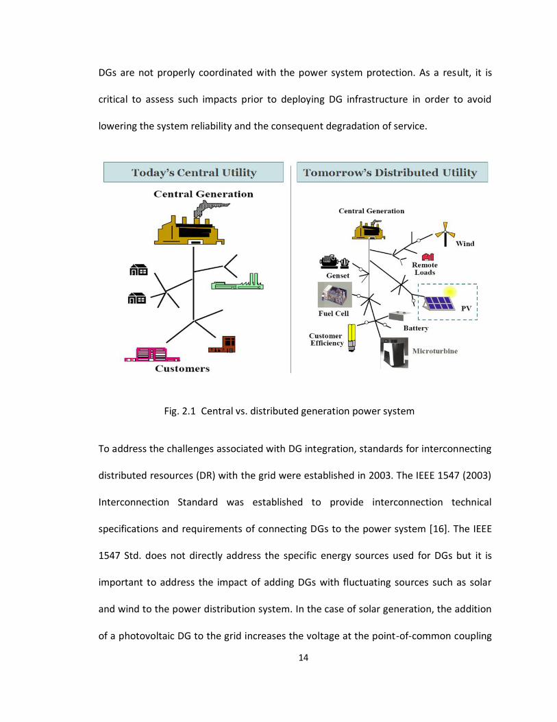
2.1 Microgrid-Embedded Power Distribution System
The power system can experience many problems when DGs are added to the existing
distribution network, mainly because the existing power system was designed to
operate in a radial manner where the power flow is unidirectional, i.e., big centralized
generating plants supplying power to loads downstream through long transmission lines
as shown in Fig. 2.1. The power grid as it is currently designed is still able to function
properly when small amounts of DGs are added to the system, but there is a limit to the
amount of new DGs that can be added to the grid before it is necessary to modify or
change some of the existing power system equipment and protection. Without proper
design and planning, the implementation of DGs in the distribution network will likely
lead to power quality problems, degradation in system reliability, reduced efficiency,
overvoltages and other safety issues [14].
The addition of DGs to the grid often results in bidirectional power flow, which can
cause problems on the existing grid configuration. So, although the application of
interconnected DGs across the power distribution system can have many positive
effects, such as grid reliability improvement through backup generation, voltage
support, as well as reducing the power losses associated with transmitting power over
long distances, it also complicates the protection schemes and associated control
equipment. For instance, the addition of DGs can adversely impact on the power quality
due to poor voltage regulation, voltage flickers, and introducing harmonics into the
power system [15]. Similarly, the reliability of the power system may be degraded if the
14
DGs are not properly coordinated with the power system protection. As a result, it is
critical to assess such impacts prior to deploying DG infrastructure in order to avoid
lowering the system reliability and the consequent degradation of service.
Fig. 2.1 Central vs. distributed generation power system
To address the challenges associated with DG integration, standards for interconnecting
distributed resources (DR) with the grid were established in 2003. The IEEE 1547 (2003)
Interconnection Standard was established to provide interconnection technical
specifications and requirements of connecting DGs to the power system [16]. The IEEE
1547 Std. does not directly address the specific energy sources used for DGs but it is
important to address the impact of adding DGs with fluctuating sources such as solar
and wind to the power distribution system. In the case of solar generation, the addition
of a photovoltaic DG to the grid increases the voltage at the point-of-common coupling
15
(PCC) between the DG and the utility grid [17, 18]. The increase in voltage can rise to
unacceptable levels if the maximum power generation of the PV coincides with light
load demand on the grid. This can lead to power system instability or cause damage to
downstream equipment. The addition of PV DGs to the grid influences the grid voltage
during normal (steady-state) operation and the voltage response during abnormal
(transient) operation [18, 19, 20].
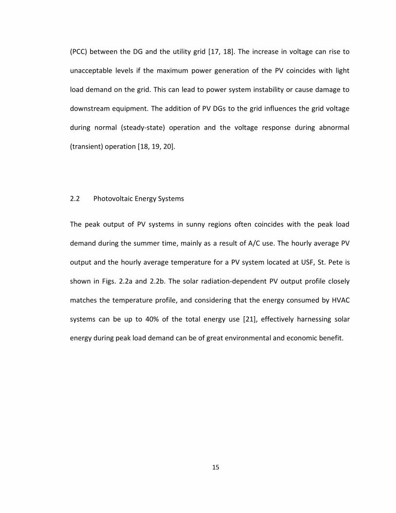
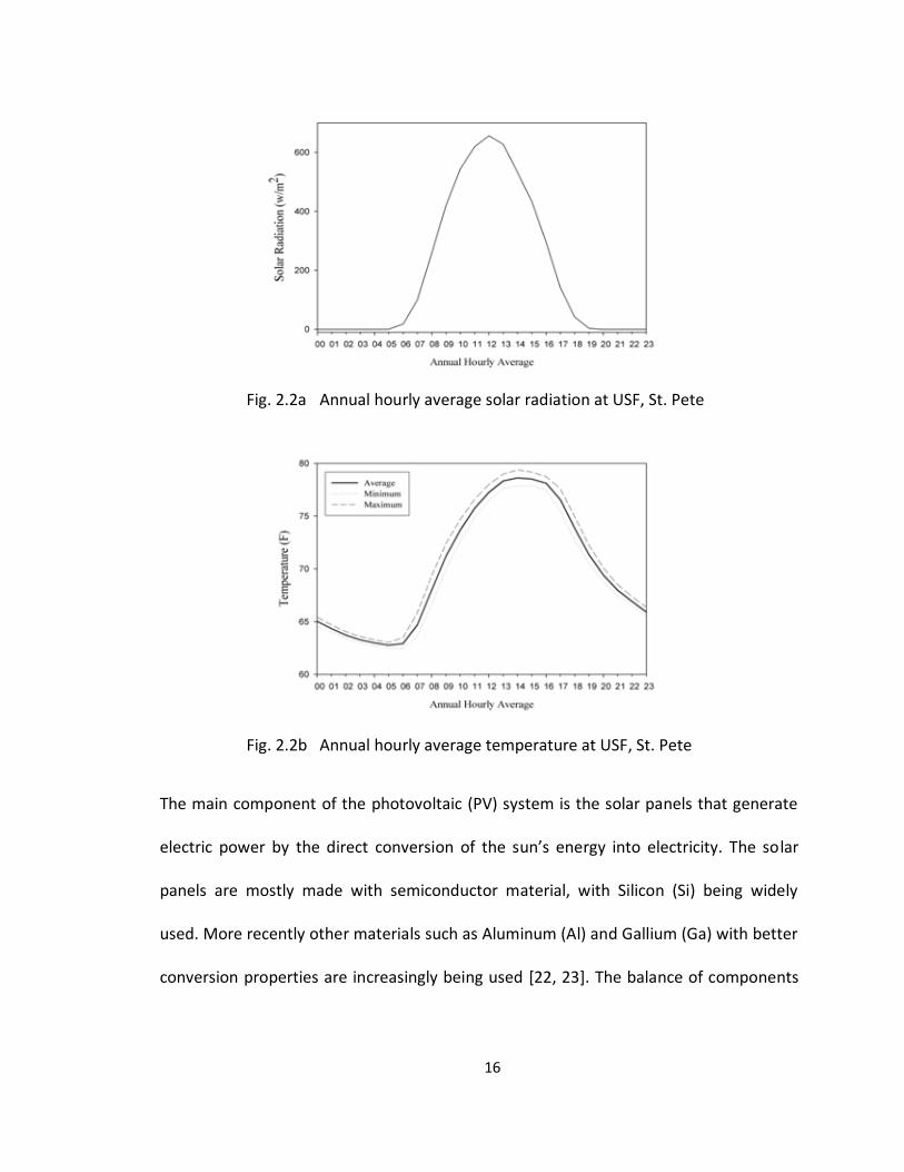
2.2 Photovoltaic Energy Systems
The peak output of PV systems in sunny regions often coincides with the peak load
demand during the summer time, mainly as a result of A/C use. The hourly average PV
output and the hourly average temperature for a PV system located at USF, St. Pete is
shown in Figs. 2.2a and 2.2b. The solar radiation-dependent PV output profile closely
matches the temperature profile, and considering that the energy consumed by HVAC
systems can be up to 40% of the total energy use [21], effectively harnessing solar
energy during peak load demand can be of great environmental and economic benefit.
16
Fig. 2.2a Annual hourly average solar radiation at USF, St. Pete
Fig. 2.2b Annual hourly average temperature at USF, St. Pete
The main component of the photovoltaic (PV) system is the solar panels that generate
electric power by the direct conversion of the sun’s energy into electricity. The solar
panels are mostly made with semiconductor material, with Silicon (Si) being widely
used. More recently other materials such as Aluminum (Al) and Gallium (Ga) with better
conversion properties are increasingly being used [22, 23]. The balance of components
17
of the PV system includes the electronic devices that interface the PV output and the AC
or DC loads.
A major challenge in utilizing solar cells for power generation is improving cell efficiency
and optimizing energy extraction. The solar cell is able to generate the maximum power
at a specific operating point, but that operating point varies depending on the ambient
conditions. This varying output effect limits the ability of utilities to predict the expected
power output at a given time for that location and thus schedule their generation
accordingly. The I-V (current-to-voltage) characteristic of the solar cell is used to
determine the operating point at which the cell generates the maximum power.
The solar cell is made of a p-n junction fabricated in a thin layer of semiconductor. The
amount of sunlight energy, referred to as photons, absorbed by the semi-conductor
material determines the output power of the solar cell. The output power is dependent
on the highly non-linear current-voltage characteristic of the semi-conductor material
shown in Fig. 2.3. The maximum power point (MPP) where the solar cell outputs the
most power can be determined from the I-V curve. The MPP power is determined by
calculating the product of the voltage and output current. The solar cell is typically
operated at or very close to the MPP in order to obtain the most power. This point is
located around the ‘bend’ or ‘knee’ of the I-V characteristic as shown at point A in Fig.
2.3.
18
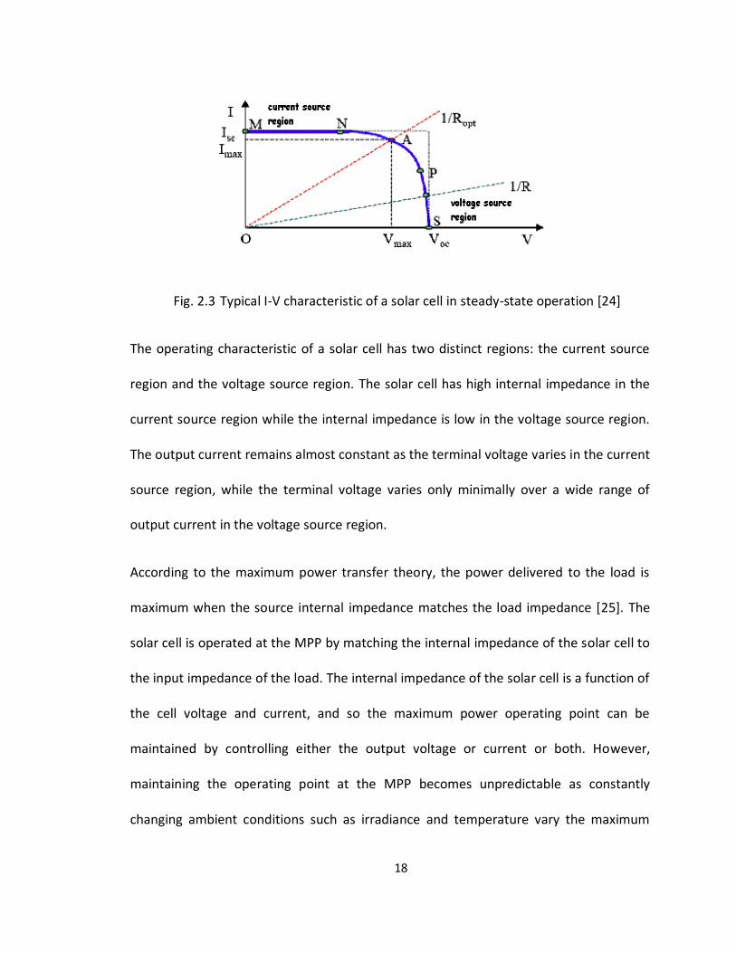
Fig. 2.3 Typical I-V characteristic of a solar cell in steady-state operation [24]
The operating characteristic of a solar cell has two distinct regions: the current source
region and the voltage source region. The solar cell has high internal impedance in the
current source region while the internal impedance is low in the voltage source region.
The output current remains almost constant as the terminal voltage varies in the current
source region, while the terminal voltage varies only minimally over a wide range of
output current in the voltage source region.
According to the maximum power transfer theory, the power delivered to the load is
maximum when the source internal impedance matches the load impedance [25]. The
solar cell is operated at the MPP by matching the internal impedance of the solar cell to
the input impedance of the load. The internal impedance of the solar cell is a function of
the cell voltage and current, and so the maximum power operating point can be
maintained by controlling either the output voltage or current or both. However,
maintaining the operating point at the MPP becomes unpredictable as constantly
changing ambient conditions such as irradiance and temperature vary the maximum
19
operating point and thus the output power. Generating the maximum power becomes a
task of tracking the MPP taking into account the varying ambient conditions. A
maximum power point tracker (MPPT) is used to accomplish the task. Most MPPT
controllers are based on the buck converter (step-down), boost converter (step-up) or
Cuk converter (buck-boost) setup [26].
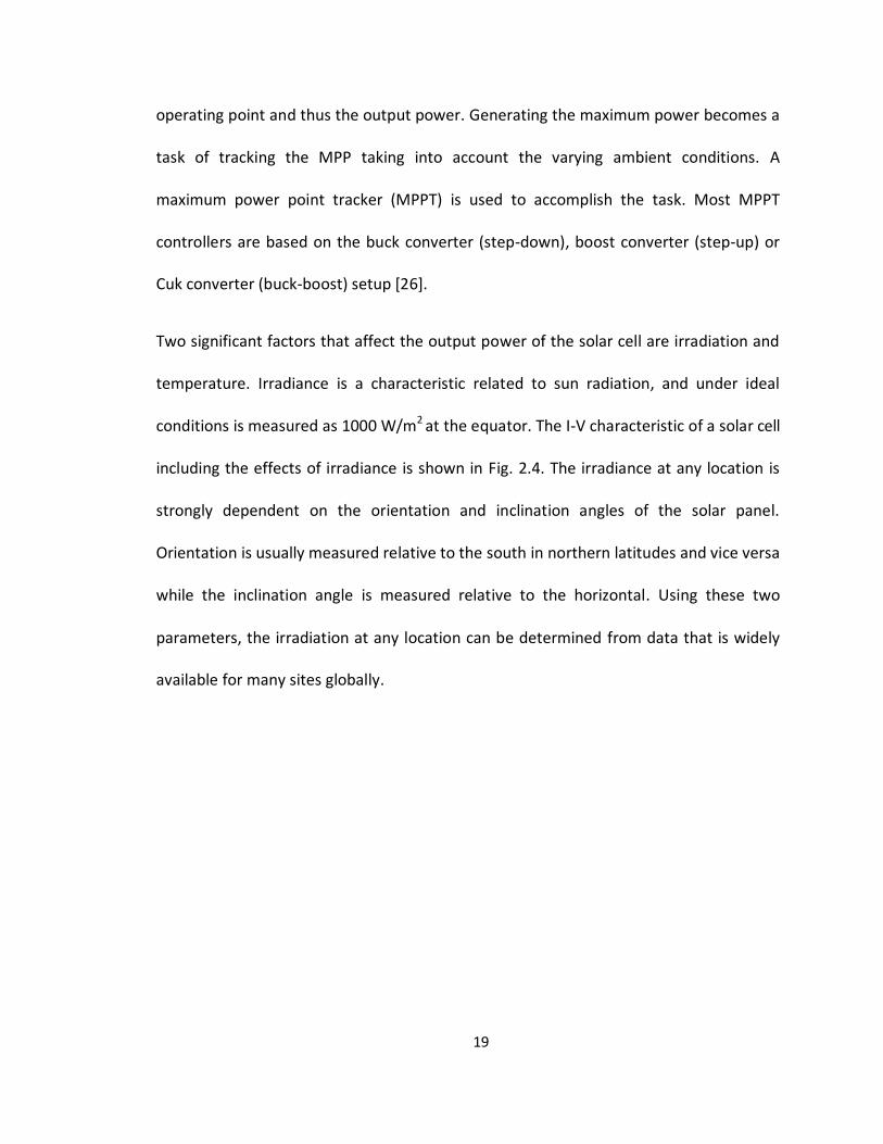
Two significant factors that affect the output power of the solar cell are irradiation and
temperature. Irradiance is a characteristic related to sun radiation, and under ideal
conditions is measured as 1000 W/m2 at the equator. The I-V characteristic of a solar cell
including the effects of irradiance is shown in Fig. 2.4. The irradiance at any location is
strongly dependent on the orientation and inclination angles of the solar panel.
Orientation is usually measured relative to the south in northern latitudes and vice versa
while the inclination angle is measured relative to the horizontal. Using these two
parameters, the irradiation at any location can be determined from data that is widely
available for many sites globally.
20
Fig. 2.4 Typical solar cell I-V characteristic showing effect of irradiance [24]
Fig. 2.4 shows that the output power is directly proportional to the irradiance. However,
it is only the output current that is affected by the irradiance. This makes sense since by
the principle of operation of the solar cell the generated current is proportional to the
flux of photons [27]. The flux of photons is greater when the sun is bright and the light
intensity is high, therefore more current is generated as the light intensity increases.
The change in voltage is minimal with varying irradiance, and for most practical
applications, the change is considered negligible [28].
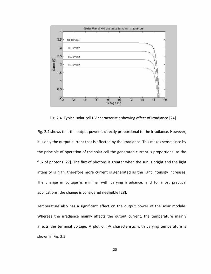
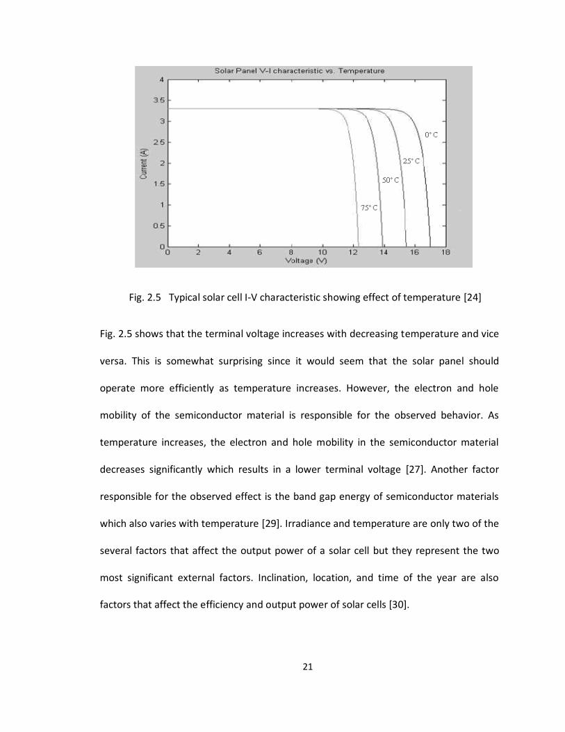
Temperature also has a significant effect on the output power of the solar module.
Whereas the irradiance mainly affects the output current, the temperature mainly
affects the terminal voltage. A plot of I-V characteristic with varying temperature is
shown in Fig. 2.5.
21
Fig. 2.5 Typical solar cell I-V characteristic showing effect of temperature [24]
Fig. 2.5 shows that the terminal voltage increases with decreasing temperature and vice
versa. This is somewhat surprising since it would seem that the solar panel should
operate more efficiently as temperature increases. However, the electron and hole
mobility of the semiconductor material is responsible for the observed behavior. As
temperature increases, the electron and hole mobility in the semiconductor material
decreases significantly which results in a lower terminal voltage [27]. Another factor
responsible for the observed effect is the band gap energy of semiconductor materials
which also varies with temperature [29]. Irradiance and temperature are only two of the
several factors that affect the output power of a solar cell but they represent the two
most significant external factors. Inclination, location, and time of the year are also
factors that affect the efficiency and output power of solar cells [30].
22
A major component in converting the power generated by the solar cell into useful
electricity is the inverter. The solar cell generates DC power while most residential,
industrial and commercial loads require AC power. Since the majority of loads are AC
loads, the DC output of the solar panels must be converted into AC voltage at system
frequency for grid-connected PV systems. An inverter is used to convert the DC power
generated by the solar cell into AC power by use of power electronic switches. The solar
cell constant current region up to the short-circuit limit makes the current output of the
solar cell ideal for current-source inverters (CSI). However, due to the fluctuating nature
of the sun and the operation of power electronic switches, a rather large reactor is
required for smoothing and blocking reverse currents [31]. As a result, voltage-source
inverters (VSI) are the most commonly used in the PV industry [32]. The voltage source
inverter can be controlled by either a voltage or current method [31 - 35], whose target
output is to output a certain voltage or current respectively.
For power system stability studies, a PV model that sufficiently represents the
significant factors that affect the dynamic output of solar cells is required to properly
study the effect of PV microgrid penetration on power system stability and reliability. In
[36], a model of PV generation system that is suitable for stability analysis is presented.
The model presented is a grid-connected system that incorporates the effect of
temperature, irradiance, and grid AC voltage in the output power and voltage of the PV.
The tracking technique implemented for the PV MPPT control in [36] is the commonly
used perturb & observe (P & O) method, but there the PV current is continuously
adjusted instead of the PV voltage as is typically the case. The PV model presented in
23
[36] is implemented in this research but with a modified tracking and control method.
Where as the model in [36] tracked the maximum power output by continuously
perturbing the operating point and comparing it to the previous iteration, with the aim
of outputting the most power based on the current grid and ambient conditions, the
control system proposed in this research controls the output power of the PV and the
output voltage of the inverter by using a deterministic method to dynamically
determine the optimal PV power and inverter voltage based on the current grid voltage
and stability margins.
2.3 Power System Stability and Reliability
Power system stability is usually classified in terms of the steady-state, dynamic or
transient stability. The steady-state stability refers to the response of the system to a
gradually increasing load; the system is said to experience steady-state instability if it is
unable to return to a state of equilibrium after a small disturbance. Gradually exceeding
the power limits of the system will cause steady-state instability [37]. The second class
of power system stability refers to the dynamic behavior of the system to oscillations.
Small disturbances regularly occur on the power system, often producing oscillations,
and the manner of those oscillations characterize the dynamic stability of the system.
Oscillations that are of successively smaller magnitudes indicate that the system is
dynamically stable, whereas if the oscillations continue to increase in magnitude, the
system experiences dynamic instability [38]. The third classification of the power system
24
stability is the transient stability. A power system is described as transiently stable, if
after a disturbance, it is able to return to equilibrium [38]. A large fault can cause a
sudden system disturbance and the ability of the power system to withstand the shock
of the large change that occurs characterizes its transient stability. Large disturbances
tend to cause large changes in rotor speed and significantly affect voltage and frequency
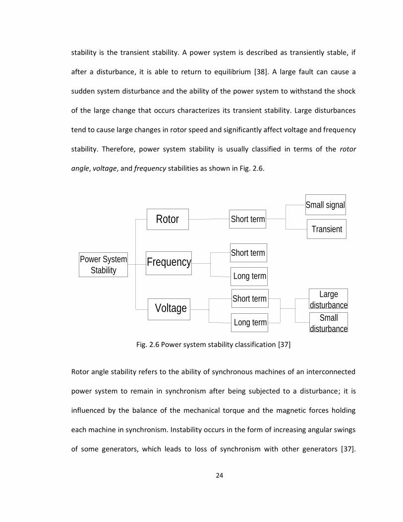
stability. Therefore, power system stability is usually classified in terms of the rotor
angle, voltage, and frequency stabilities as shown in Fig. 2.6.
Rotor
FrequencyPower System
Stability
Short term
Small signal
Transient
Short term
Long term
VoltageShort term
Long term
Large
disturbance
Small
disturbance
Fig. 2.6 Power system stability classification [37]
Rotor angle stability refers to the ability of synchronous machines of an interconnected
power system to remain in synchronism after being subjected to a disturbance; it is
influenced by the balance of the mechanical torque and the magnetic forces holding
each machine in synchronism. Instability occurs in the form of increasing angular swings
of some generators, which leads to loss of synchronism with other generators [37].
25
There are two types of rotor angle instability, depending on the size of the disturbance.
The small signal disturbance (small disturbance) stability refers to the ability of the
power system to maintain synchronism under small disturbances, such as a gradual
increase in load while the transient (large disturbance) stability refers to the ability of
the system to maintain synchronism under large disturbances, such as a large fault.
Small signal stability is usually affected by insufficient damping torque, which results in
small disturbances having oscillations of increasing magnitude and a loss of equilibrium.
For relatively small disturbances, where the duration of interest is on the order of 10 to
20 seconds post disturbance, it is permissible to analyze the small signal stability using
linearized models [38]. On the other hand, transient stability is highly influenced by the
non-linear power angle relationship, and linearized models are not suitable for analysis
[39]. Instead the analysis is done using non-linear time-domain simulations, where the
duration of interest is three to five seconds post disturbance.
Frequency stability refers to the ability of a power system to maintain steady frequency,
within acceptable range, following a severe system disturbance that causes significant
imbalance between generation and load; it is influenced by the ability of the system to
maintain balance between generation and load demand. Instability occurs in the form of
sustained frequency swings, leading to generators and/or loads being switched off [37].
Unlike rotor angle and voltage stabilities, frequency stability is not classified based on
the size of the system disturbance but rather on the overall response of the system. It
can be described as a short or long term phenomenon as shown in Fig. 2.6.
26
Voltage stability refers to the ability of the system, normally operating, to maintain
steady voltages at all buses after being subjected to a disturbance. It is influenced by the
balance between load demand and supply. Instability occurs in the form of progressive
drop in voltage at some buses. The system experiences voltage instability if at any bus,
there is a drop in voltage as the reactive power is increased [38]. Similar to the rotor
angle stability, the small signal voltage stability and the large disturbance voltage
stability refer to the system’s ability to maintain steady voltages at all buses when
subjected to small and large disturbances respectively. A small disturbance may be a
gradual increase in load or momentary voltage sag while a large sustained system fault
would constitute a large disturbance. After a disturbance occurs on the systems, loads
tend to be quickly restored on the power system as a result of the operation of
automatic controllers such as auto-starters in induction motors. The sudden increase in
reactive power consumption by the load worsens the voltage sag caused by the
disturbance and the load reacts by further increasing the reactive power consumption.
This process continues until the stability limit of the system is exceeded, resulting in
voltage collapse or even widespread blackout. Some of the system parameters that
influence the stability limit of the power system include the generation capacity and the
network transfer capacity [40]. But loads are the primary drivers in voltage instability.
The duration of interest in voltage stability studies may run from a few seconds to
several minutes after the disturbance. Since voltage stability depends on both linear and
non-linear characteristics of the system, a combination of both techniques is used for
analysis.
27
Rotor angle stability can be viewed as a generator stability issue; voltage stability as a
load issue; and frequency stability as a combination of generator and load balance. For
this reason, the rotor angle stability is primarily influenced by real power transfer while
voltage stability is mainly influenced by reactive power flow. A point to note is that it is
possible for more than one type of instability to occur on the system at a given time,
and therefore power system stability studies should be performed in the context of
overall system stability.
Utilities are concerned with both the stability and reliability of the power supplied to
customers. The reliability of power supply is measured by reliability indices that are
recognized throughout the industry. Utilities are required to report and publish their
yearly reliability indices, and they are subject to penalties if their performance fails to
meet certain criteria. The indices indicate the annual average performance of the
utilities based on the duration and frequency of interruptions to customers. The system
performance indices are [41] described below.
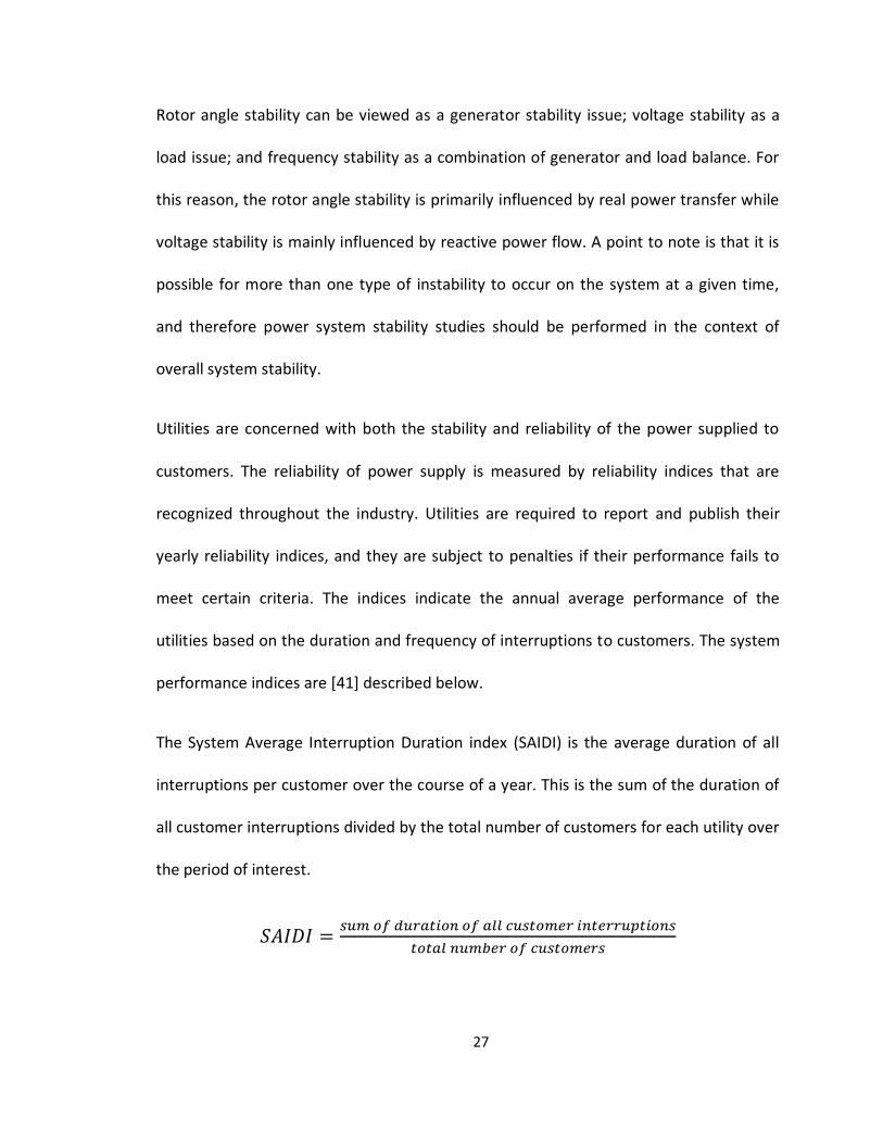
The System Average Interruption Duration index (SAIDI) is the average duration of all
interruptions per customer over the course of a year. This is the sum of the duration of
all customer interruptions divided by the total number of customers for each utility over
the period of interest.
28
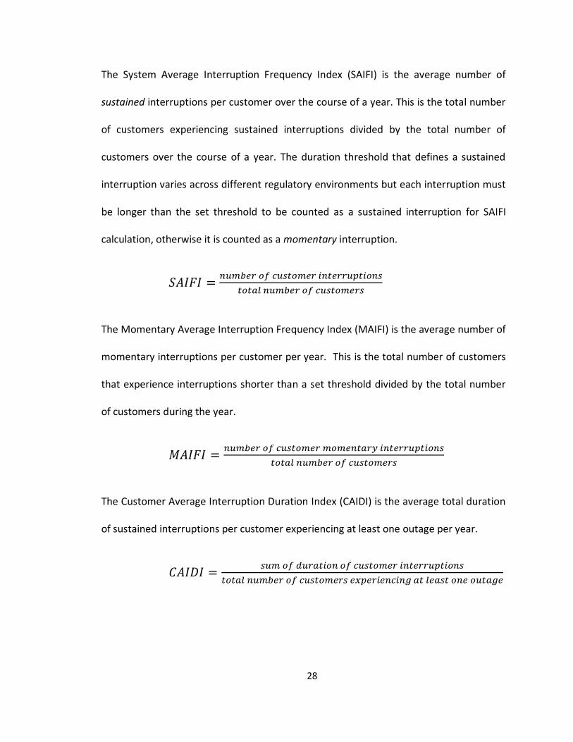
The System Average Interruption Frequency Index (SAIFI) is the average number of
sustained interruptions per customer over the course of a year. This is the total number
of customers experiencing sustained interruptions divided by the total number of
customers over the course of a year. The duration threshold that defines a sustained
interruption varies across different regulatory environments but each interruption must
be longer than the set threshold to be counted as a sustained interruption for SAIFI
calculation, otherwise it is counted as a momentary interruption.
The Momentary Average Interruption Frequency Index (MAIFI) is the average number of
momentary interruptions per customer per year. This is the total number of customers
that experience interruptions shorter than a set threshold divided by the total number
of customers during the year.
The Customer Average Interruption Duration Index (CAIDI) is the average total duration
of sustained interruptions per customer experiencing at least one outage per year.
29
These indices are used by the regulator to measure the performance of the utilities’
network and ensure a minimum level of service is attained. The regulator may apply
fines or suggest remedial action to improve the quality of service.
2.4 Momentary Interruptions and Voltage Sags
Momentary interruptions are brief disruptions in electric service that are usually caused
by faults in the power distribution system. These interruptions are more noticeable now
due to the increase in the use of sensitive power electronics equipment, while the cost
of these interruptions is a major source of concern for utilities and customers. The total
annual cost to US electricity customers as a result of interruptions in service is about
$250 billion and rising, with momentary interruptions accounting for two-thirds of the
overall cost [42]. In general, power quality disturbances refer to the deviations of the
voltage and current from their ideal waveforms that can cause interruptions, tripping of
equipment or improper power system operation. Voltage variations, such as momentary
interruptions and voltage sags cause motors to run hard and overheat quickly, and while
not always noticeable, can result in long-term damage to equipment. Voltage sags are
characterized by short duration changes in rms voltage magnitude at the receiving end.
IEEE Std. 1159 classifies an rms voltage disturbance based upon its duration and voltage
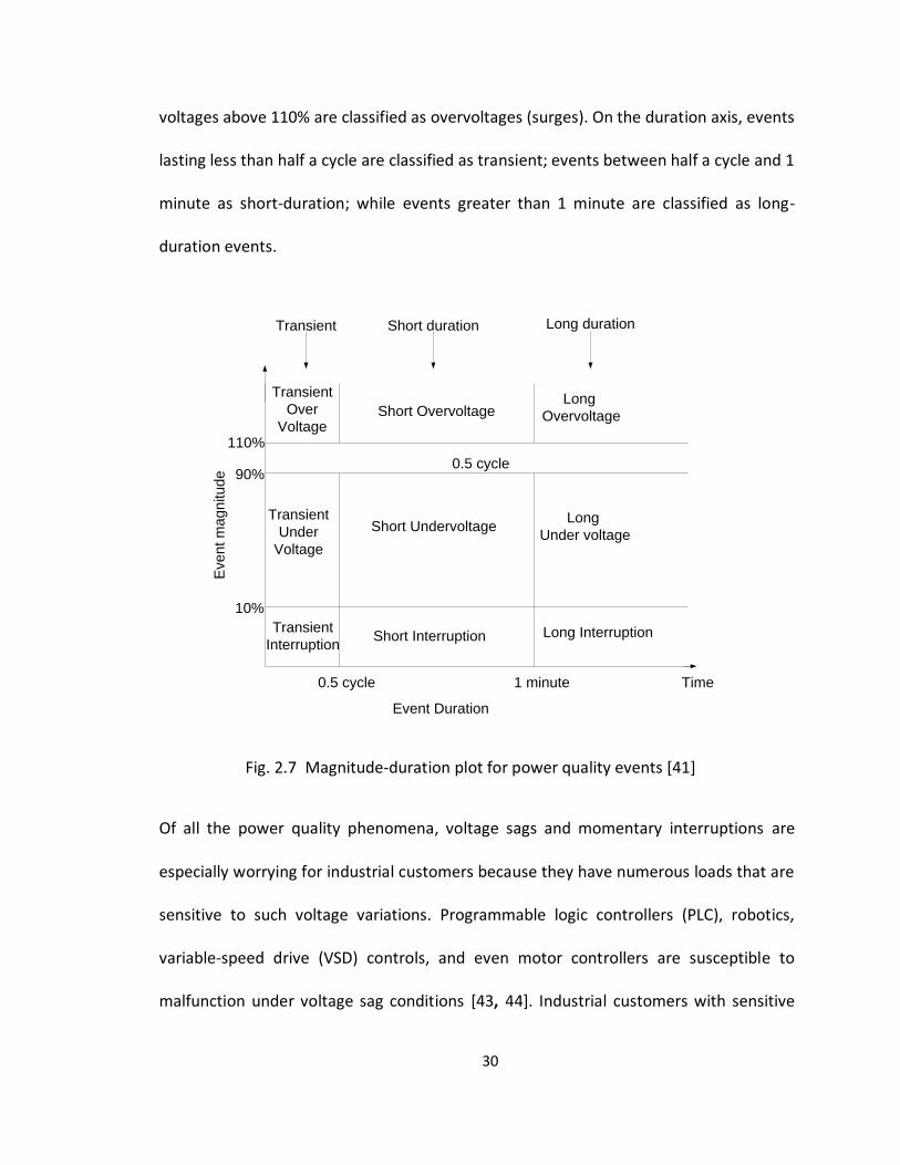
magnitude. A magnitude-duration plot used in IEEE Std. 1159 is shown in Fig. 2.7. On
the voltage magnitude axis, voltages less than 10% of nominal voltages are classified as
interruptions; voltages between 10% and 90% are classified as undervoltages (sags); and
30
voltages above 110% are classified as overvoltages (surges). On the duration axis, events
lasting less than half a cycle are classified as transient; events between half a cycle and 1
minute as short-duration; while events greater than 1 minute are classified as long-
duration events.
Transient
Over
VoltageShort Overvoltage
Long
Overvoltage
Event Duration
Transient
Under
Voltage
Short UndervoltageLong
Under voltage
Transient
InterruptionShort Interruption Long Interruption
Time
Eve
nt m
ag
nitu
de
110%
90%
10%
0.5 cycle 1 minute
0.5 cycle
Transient Short duration Long duration
Fig. 2.7 Magnitude-duration plot for power quality events [41]
Of all the power quality phenomena, voltage sags and momentary interruptions are
especially worrying for industrial customers because they have numerous loads that are
sensitive to such voltage variations. Programmable logic controllers (PLC), robotics,
variable-speed drive (VSD) controls, and even motor controllers are susceptible to
malfunction under voltage sag conditions [43, 44]. Industrial customers with sensitive

31
process equipment, such as semi-conductor manufacturing facilities or medical facilities
using MRI and CTs machines, often have to restart or reprogram the machine as a result
of voltage sags, while work-in-process wafers or scans may need to be scrapped. As a
result, there is a concerted effort in industry to reduce the number of momentary
interruptions in the power system, measured by the MAIFI index.
2.5 Recent MAIFI Performance Indicators for Florida Utilities
The Florida Public Service Commission (PSC) publishes annual MAIFI scores for the four
largest utilities in Florida: Florida Power & Light (FPL), Progress Energy Florida (PEF),
Tampa Electric Co. (TECO), and Gulf Power Co. (Gulf) with approximately 4.5 million, 1.6
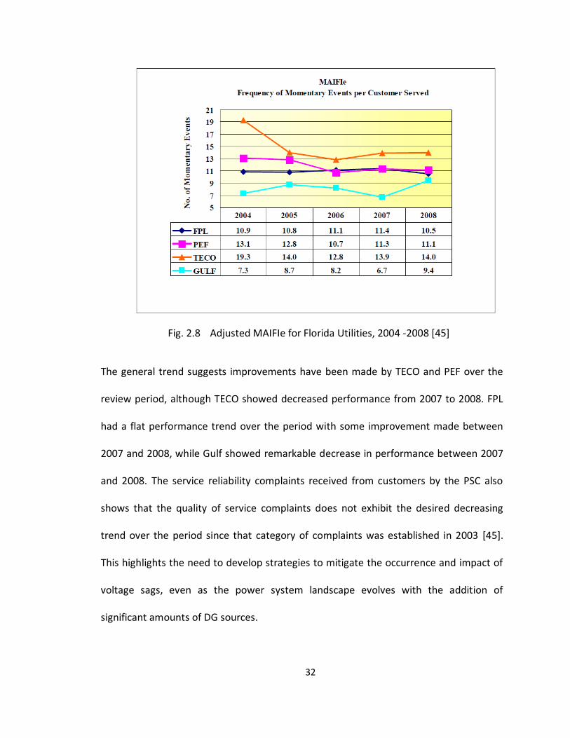
million, 670,000, and 430,000 customers respectively. The adjusted MAIFI for years
2004 -2008 is shown in Fig. 2.8.
32
Fig. 2.8 Adjusted MAIFIe for Florida Utilities, 2004 -2008 [45]
The general trend suggests improvements have been made by TECO and PEF over the
review period, although TECO showed decreased performance from 2007 to 2008. FPL
had a flat performance trend over the period with some improvement made between
2007 and 2008, while Gulf showed remarkable decrease in performance between 2007
and 2008. The service reliability complaints received from customers by the PSC also
shows that the quality of service complaints does not exhibit the desired decreasing
trend over the period since that category of complaints was established in 2003 [45].
This highlights the need to develop strategies to mitigate the occurrence and impact of
voltage sags, even as the power system landscape evolves with the addition of
significant amounts of DG sources.
33
2.6 Various Voltage Sag Mitigation Methods
Voltage sags and momentary interruptions adversely affect the power quality
experienced by electricity customers. Increased load sensitivity and production
automation are two of the major factors driving interest and concerted efforts to
mitigate the occurrence and impact of voltage sags [46]. The methods applied to
mitigate the problem occur at the utility, customer and equipment manufacturers’
levels. Sensitive electronic equipment are designed with a greater tolerance to voltage
sags while the customer can install voltage regulating equipment such as uninterrupted
power supply (UPS), dynamic voltage restorer (DVR) or coil hold-in devices near
sensitive loads to protect the equipment. The utility is primarily focused on maintaining
the stability of the overall power system, thus the utility attempts to first maintain a
balance between demand and supply, then ensure that the voltage at all buses in the
power system are maintained within a desired range. In the case where the demand
exceeds the supply, the utility is forced to shed non-critical loads in order to avoid
power system instability and voltage collapse [47].
The criteria for voltage stability margin for load shedding purposes proposed in [47] only
deals with load shedding at the sub-station after the system has experienced a severe
disturbance leading to voltage collapse. In order to forestall voltage collapse, the utility
installs reactive power compensation devices such as shunt capacitors, STATCOMs, SVCs
and FACTS devices in the power distribution system to support the voltage at weak
buses [48]. However, there is a limit to the number of locations where these devices can
34
be reasonably installed mainly due to the associated cost and low utilization factor.
Devices deployed at locations that require voltage compensation during peak hours only
can remain idle for up to 20 hours each day, therefore costly SVCs and FACTS devices
are usually only deployed at critical locations where quick voltage regulation is required
[49].
Recently, distribution generation has been explored as a solution to mitigate voltage
sags in the low-voltage distribution network [50]. The impact of grid-connected DG units
during voltage sags is investigated in [51] for asynchronous generators, synchronous
generators and converter-connected DG units. The impact of commercially available
converter-connected DG is reported to be negligible since most converters operate at
unity power factor and the current injected into the grid is limited to the nominal
current of the inverter [51]. A method to control the converter-connected units to
obtain a better voltage sag ride-through capability is presented in [52]. The controller
employs damping resistance to prevent premature shutdown of the converter due to
excessive bus voltage when the injected power is increased to counter the voltage sag.
However, this approach has limited application for deep voltage sags at buses
containing a high number of induction motors where the converter shuts down due to
excessive bus voltage, since only the active power injection is regulated and the voltage
at the PCC exceeds acceptable limits before the voltage at the motor terminals recover.
A method to operate grid-tied DGs to individually regulate both the active and reactive
power injection into the load bus is presented in this work. The impact of such

35
converter-connected DGs during voltage sags is investigated and the outcome is
compared to the results obtained in [51]. The method improves on the approach
presented in [52] by dynamically regulating the reactive power injection of the
converter during voltage sags thus preventing the excessive bus voltage that results
primarily from the active power injection at the load.

36
3. MICROGRID IMPACT ON POWER SYSTEM VOLTAGE STABILITY
The power system generally experiences voltage instability when there is a real and/or
reactive power imbalance between the generators and the loads. The reasons for the
static and dynamic voltage instability of a power system are investigated in this chapter.
The basic concepts related to voltage instability are illustrated by firstly considering the
characteristics of the transmission and distribution systems and then examining how the
phenomenon is influenced by the behavior of generators, loads, and reactive power
compensation equipment. The voltage stability behavior of the power system changes
significantly when distributed resources are added to the grid as a result of the
reconfiguration of the power flow. Therefore, prior to deploying DGs in the power
system, it is necessary to properly model and analyze the impact of adding DGs at
different locations in the grid. The standard mathematical models of the various power
system components, including the synchronous generator and photovoltaic source, are
presented and implemented in Matlab/Simulink. The implemented models are used to
determine the effect of grid-connected PV sources on local voltage regulation and
power system reliability. Some remedial actions such as dynamic voltage regulation and
active anti-islanding that can be implemented to prevent overvoltages and nuisance
fuse operation are explored and presented.
37
3.1 Power Flow in Radial Power Systems
The power system can experience instability when there is an imbalance between the
load demand and the capacity of the power system to provide sufficient power to the
loads from the generation and transmission ends. However, the power flow in the
emerging DG-embedded power system varies significantly from the power flow in the
traditional radial power system since the sources and loads are much closer in proximity
in the former than in the latter. With the shifting paradigm, the effect of the new
configuration of the power system on voltage stability at the distribution level needs to
be investigated to ensure the proper design and optimal placement of microgrids in the
power system. The power flow in a short transmission line is used to illustrate the
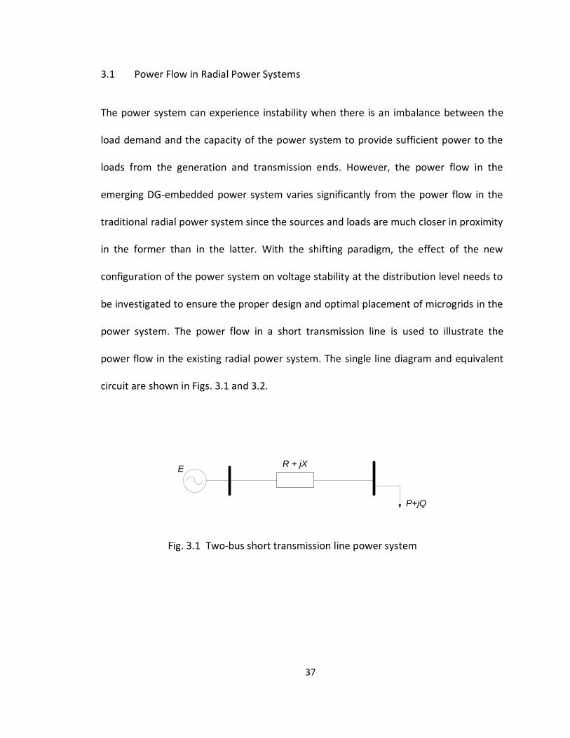
power flow in the existing radial power system. The single line diagram and equivalent
circuit are shown in Figs. 3.1 and 3.2.
P+jQ
R + jXE
Fig. 3.1 Two-bus short transmission line power system

38
(a) (b)
Fig. 3.2 a) Equivalent circuit of a short transmission system and, b) phasor
relationship between source and load voltage
We assume the transmission line shown has negligible resistance and the series
impedance is jX Ω/phase. The source and load side voltages are ES and VL respectively. It
is known that VL lags ES as shown in Fig. 3.2.
The real and reactive power and reactive power at the source and load can be
determined using the phasor relationship:
The total power S is given by
[VA] (3.1)
At the source,
[VA] (3.2)
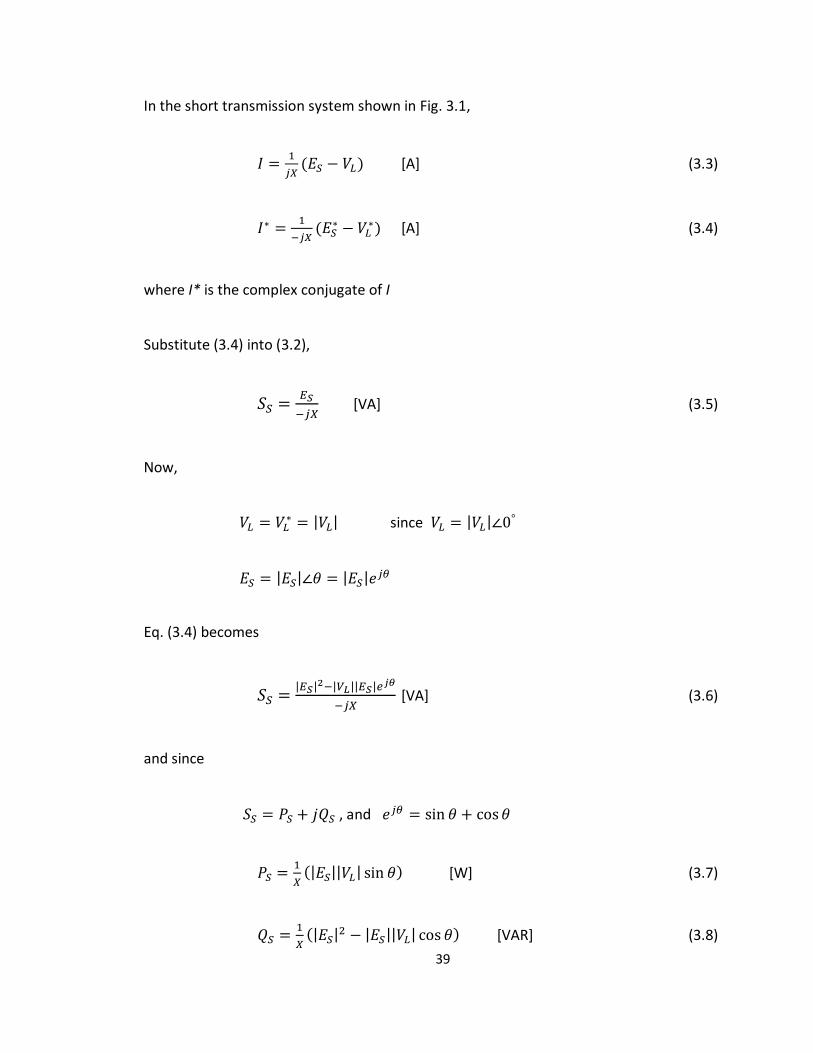
39
In the short transmission system shown in Fig. 3.1,
[A] (3.3)
[A] (3.4)
where I* is the complex conjugate of I
Substitute (3.4) into (3.2),
[VA] (3.5)
Now,
since
Eq. (3.4) becomes
[VA] (3.6)
and since
, and
[W] (3.7)
[VAR] (3.8)
40
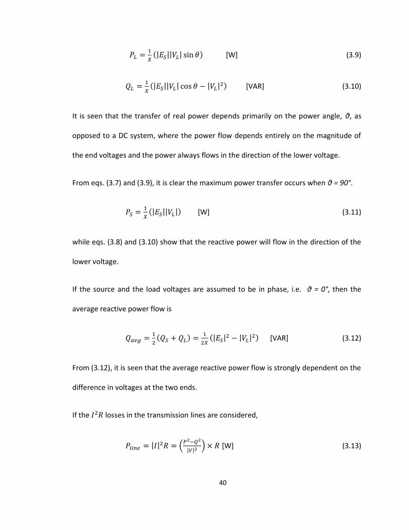
[W] (3.9)
[VAR] (3.10)
It is seen that the transfer of real power depends primarily on the power angle, θ, as
opposed to a DC system, where the power flow depends entirely on the magnitude of
the end voltages and the power always flows in the direction of the lower voltage.
From eqs. (3.7) and (3.9), it is clear the maximum power transfer occurs when θ = 90°.
[W] (3.11)
while eqs. (3.8) and (3.10) show that the reactive power will flow in the direction of the
lower voltage.
If the source and the load voltages are assumed to be in phase, i.e. θ = 0°, then the
average reactive power flow is
[VAR] (3.12)
From (3.12), it is seen that the average reactive power flow is strongly dependent on the
difference in voltages at the two ends.
If the losses in the transmission lines are considered,
[W] (3.13)

41
Eq. (3.13) shows that the power loss in the transmission line is dependent on both real
and reactive power. The simplified transmission line shown in Fig. 3.1 shows the effect
of the reactive power flow when transferring power from one end of the transmission
system to the other in a typical vertical power system. This dependence of the reactive
power flow on voltage magnitudes allows the bus voltage to be maintained at a desired
level by controlling the flow of reactive power to the bus.
3.2 Impact of Voltage Regulating Devices
Four of the most common methods currently used to control the amount of reactive
power in the system, and thus regulate the voltage, include –
adjusting synchronous generators or motor field excitation
using shunt capacitors
using FACTS devices
using load-tap-changing (LTC) transformers
Synchronous generators are the main source of reactive power in the power system,
and thus are largely responsible for maintaining a good voltage profile across the power
system. In order to maintain system stability, all the synchronous generators must
remain in synchronism [53]. The equation governing the rotor motion of the generator
is given as [54]:
42
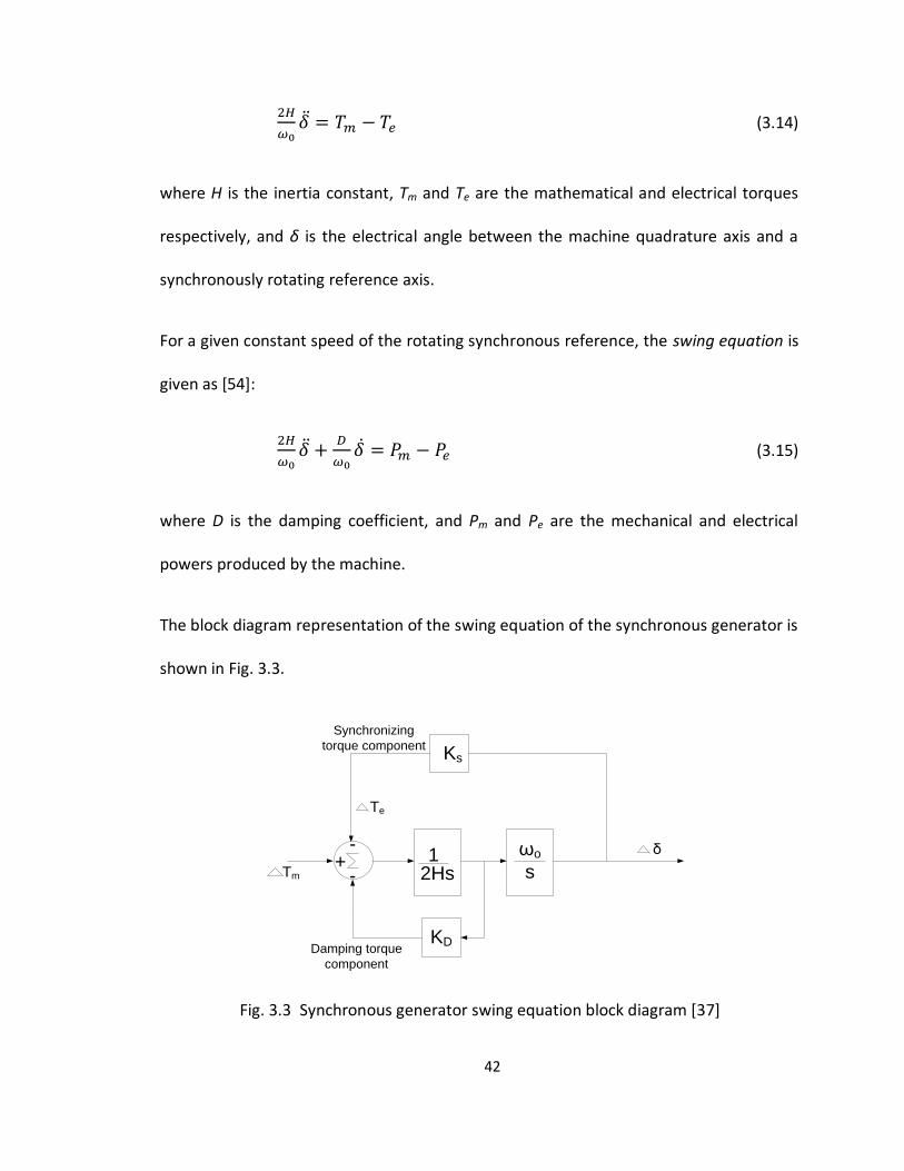
(3.14)
where H is the inertia constant, Tm and Te are the mathematical and electrical torques
respectively, and δ is the electrical angle between the machine quadrature axis and a
synchronously rotating reference axis.
For a given constant speed of the rotating synchronous reference, the swing equation is
given as [54]:
(3.15)
where D is the damping coefficient, and Pm and Pe are the mechanical and electrical
powers produced by the machine.
The block diagram representation of the swing equation of the synchronous generator is
shown in Fig. 3.3.
12Hs
+-
-
Ks
KD
Tm
Damping torque
component
Te
Synchronizing
torque component
ωo δ
s
Fig. 3.3 Synchronous generator swing equation block diagram [37]
43
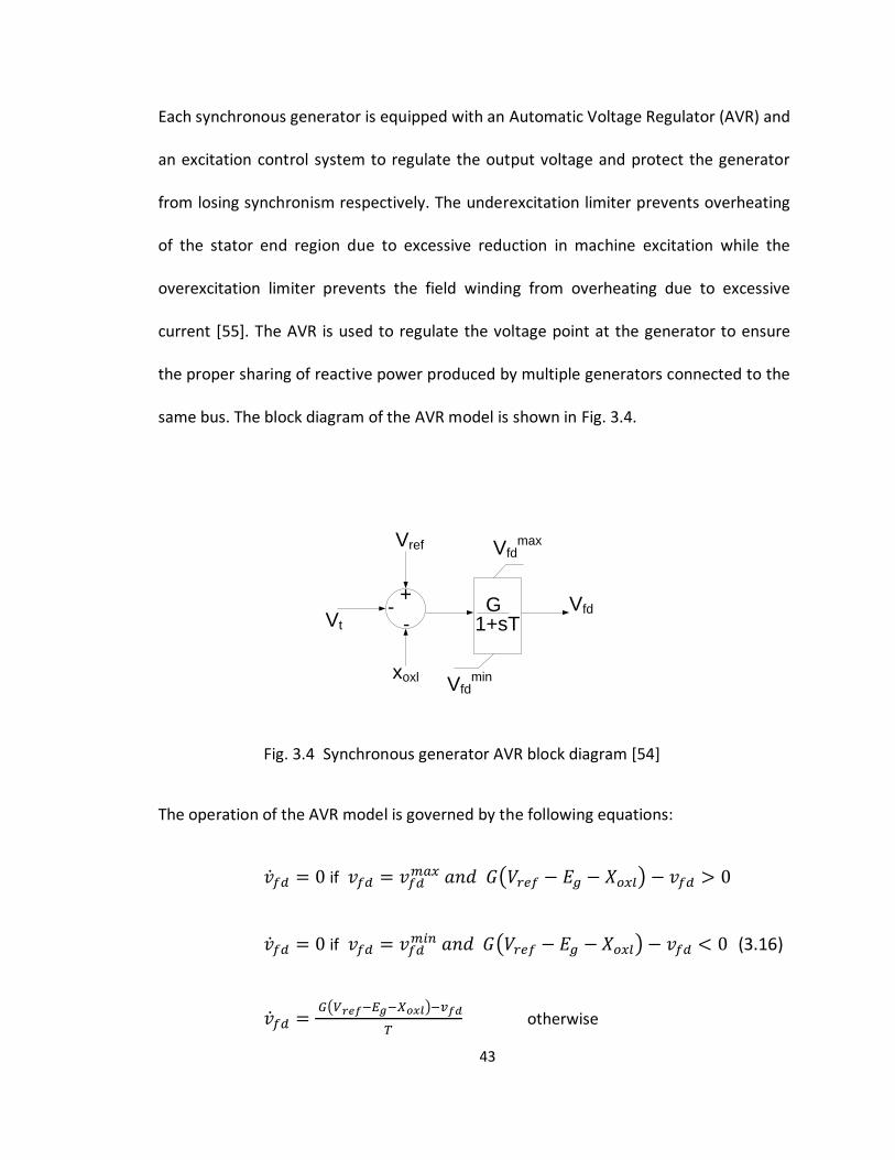
Each synchronous generator is equipped with an Automatic Voltage Regulator (AVR) and
an excitation control system to regulate the output voltage and protect the generator
from losing synchronism respectively. The underexcitation limiter prevents overheating
of the stator end region due to excessive reduction in machine excitation while the
overexcitation limiter prevents the field winding from overheating due to excessive
current [55]. The AVR is used to regulate the voltage point at the generator to ensure
the proper sharing of reactive power produced by multiple generators connected to the
same bus. The block diagram of the AVR model is shown in Fig. 3.4.
G1+sT
+
-- Vfd
Vfdmax
Vfdmin
Vt
Vref
xoxl
Fig. 3.4 Synchronous generator AVR block diagram [54]
The operation of the AVR model is governed by the following equations:
if
if (3.16)
otherwise
44
where and
are the minimum and maximum field voltages respectively. Eg
and Vref are the generator and AVR reference voltages respectively. G and T are the AVR
gain and time constants respectively while Xoxl is the output of the overexcitation
limiter.
The set of differential equations that govern the dynamics of the synchronous generator
is given as [56]:
(3.17)
(3.18)
(3.19)
where is the voltage behind the transient reactance, vfd is the field voltage at the
armature, is the open circuit time constant, and id is the direct-axis armature
current. and are the direct axis reactance and transient reactance respectively.
Eg
Q
jX
V0= 1 p.u.
Fig. 3.5 Increase in synchronous generator field excitation
45
Increasing the field excitation on a synchronous generator will result in an increase in
the magnitude of the generator voltage, , as shown in Fig. 3.5. The generator is
assumed to be connected to a bus operating at a voltage of 1 0° p.u. The magnitude of
generator can be increased or decreased by raising or lowering the generator or
motor field current. If the real power flow is neglected and only the reactive power flow
is considered, then the average power flow is proportional to Therefore,
for a synchronous generator or unloaded synchronous motor, increasing the field
excitation will result in reactive power flow into the system bus as shown in Fig. 3.5. This
causes an increase in the voltage at the bus.
Shunt capacitors are used to control the bus voltage by supplying reactive power to the
bus at which the capacitor banks are connected. The shunt capacitors supply reactive
power to the load thereby reducing the inductive reactance seen at the generator by
way of power factor correction. This reduces the line current necessary to supply the
load, resulting in lower voltage drop and losses in the line. However, this approach
to reactive power control becomes counterproductive if too much capacitance is added
as the line current leads the voltage and the VARs begin to rise again. The static on/off
switching of capacitors can also introduce significant harmonics and in-rush currents
into the load, and therefore switching capacitors around extremely sensitive equipment
often require additional design complexity.
Flexibles alternating current transmission system (FACTS) devices such as Static VAR
compensators (SVC) and static synchronous compensators (STATCOM) involve using
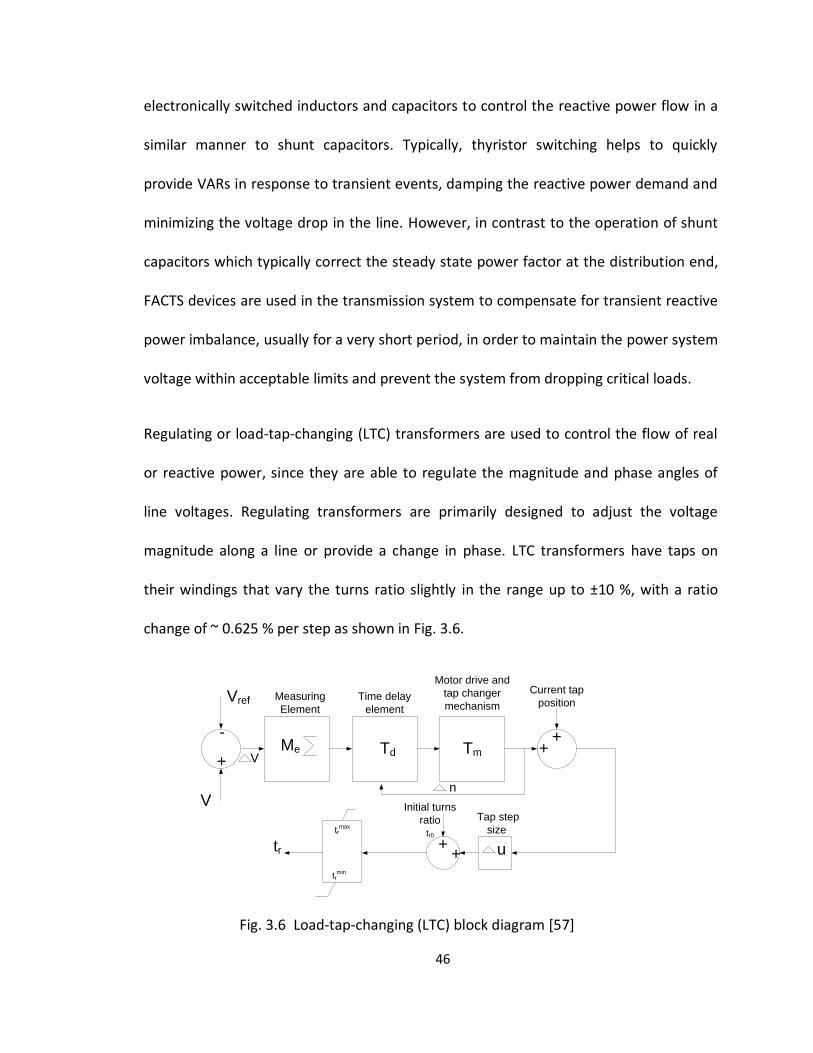
46
electronically switched inductors and capacitors to control the reactive power flow in a
similar manner to shunt capacitors. Typically, thyristor switching helps to quickly
provide VARs in response to transient events, damping the reactive power demand and
minimizing the voltage drop in the line. However, in contrast to the operation of shunt
capacitors which typically correct the steady state power factor at the distribution end,
FACTS devices are used in the transmission system to compensate for transient reactive
power imbalance, usually for a very short period, in order to maintain the power system
voltage within acceptable limits and prevent the system from dropping critical loads.
Regulating or load-tap-changing (LTC) transformers are used to control the flow of real
or reactive power, since they are able to regulate the magnitude and phase angles of
line voltages. Regulating transformers are primarily designed to adjust the voltage
magnitude along a line or provide a change in phase. LTC transformers have taps on
their windings that vary the turns ratio slightly in the range up to ±10 %, with a ratio
change of ~ 0.625 % per step as shown in Fig. 3.6.
+
-
utrtr0
V
Vref
Td Tm
+
Current tap
position
Tap step
size
Initial turns
ratio
Me
Motor drive and
tap changer
mechanismTime delay
element
Measuring
Element
V
trmax
trmin
+
n
+
+
Fig. 3.6 Load-tap-changing (LTC) block diagram [57]
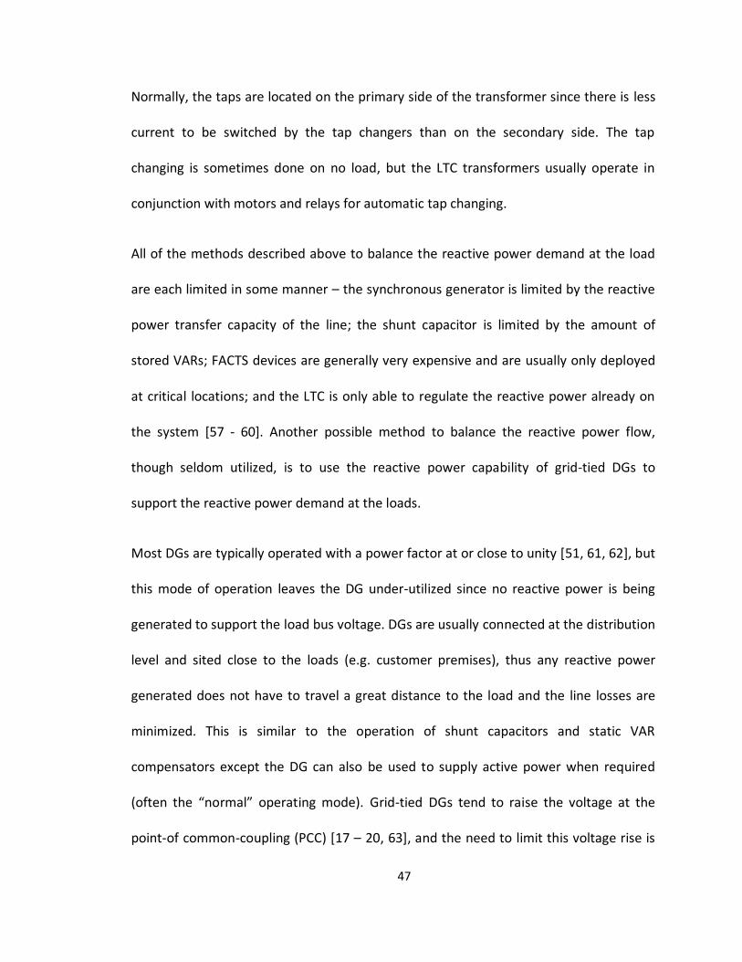
47
Normally, the taps are located on the primary side of the transformer since there is less
current to be switched by the tap changers than on the secondary side. The tap
changing is sometimes done on no load, but the LTC transformers usually operate in
conjunction with motors and relays for automatic tap changing.
All of the methods described above to balance the reactive power demand at the load
are each limited in some manner – the synchronous generator is limited by the reactive
power transfer capacity of the line; the shunt capacitor is limited by the amount of
stored VARs; FACTS devices are generally very expensive and are usually only deployed
at critical locations; and the LTC is only able to regulate the reactive power already on
the system [57 - 60]. Another possible method to balance the reactive power flow,
though seldom utilized, is to use the reactive power capability of grid-tied DGs to
support the reactive power demand at the loads.
Most DGs are typically operated with a power factor at or close to unity [51, 61, 62], but
this mode of operation leaves the DG under-utilized since no reactive power is being
generated to support the load bus voltage. DGs are usually connected at the distribution
level and sited close to the loads (e.g. customer premises), thus any reactive power
generated does not have to travel a great distance to the load and the line losses are
minimized. This is similar to the operation of shunt capacitors and static VAR
compensators except the DG can also be used to supply active power when required
(often the “normal” operating mode). Grid-tied DGs tend to raise the voltage at the
point-of common-coupling (PCC) [17 – 20, 63], and the need to limit this voltage rise is
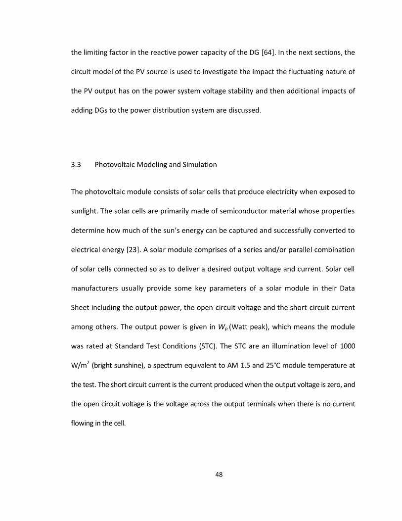
48
the limiting factor in the reactive power capacity of the DG [64]. In the next sections, the
circuit model of the PV source is used to investigate the impact the fluctuating nature of
the PV output has on the power system voltage stability and then additional impacts of
adding DGs to the power distribution system are discussed.
3.3 Photovoltaic Modeling and Simulation
The photovoltaic module consists of solar cells that produce electricity when exposed to
sunlight. The solar cells are primarily made of semiconductor material whose properties
determine how much of the sun’s energy can be captured and successfully converted to
electrical energy [23]. A solar module comprises of a series and/or parallel combination
of solar cells connected so as to deliver a desired output voltage and current. Solar cell
manufacturers usually provide some key parameters of a solar module in their Data
Sheet including the output power, the open-circuit voltage and the short-circuit current
among others. The output power is given in Wp (Watt peak), which means the module
was rated at Standard Test Conditions (STC). The STC are an illumination level of 1000
W/m2 (bright sunshine), a spectrum equivalent to AM 1.5 and 25°C module temperature at
the test. The short circuit current is the current produced when the output voltage is zero, and
the open circuit voltage is the voltage across the output terminals when there is no current
flowing in the cell.
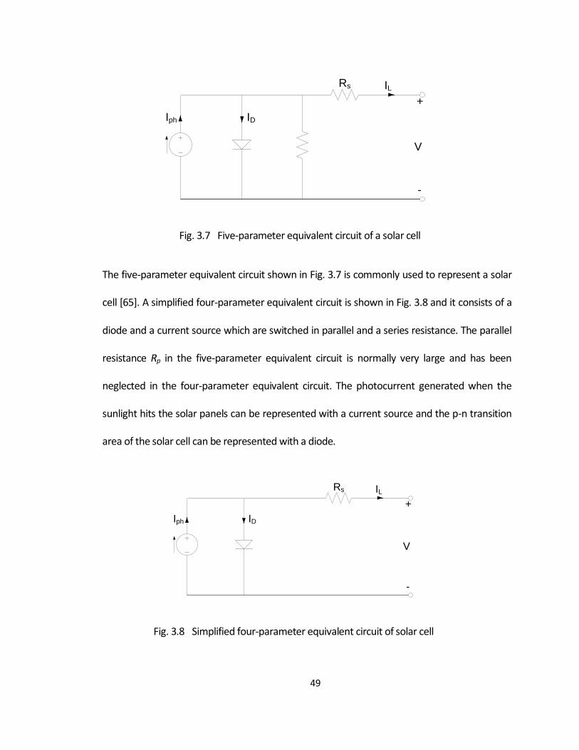
49
V
Rs IL
IDIph
+
-
Fig. 3.7 Five-parameter equivalent circuit of a solar cell
The five-parameter equivalent circuit shown in Fig. 3.7 is commonly used to represent a solar
cell [65]. A simplified four-parameter equivalent circuit is shown in Fig. 3.8 and it consists of a
diode and a current source which are switched in parallel and a series resistance. The parallel
resistance Rp in the five-parameter equivalent circuit is normally very large and has been
neglected in the four-parameter equivalent circuit. The photocurrent generated when the
sunlight hits the solar panels can be represented with a current source and the p-n transition
area of the solar cell can be represented with a diode.
V
Rs IL
IDIph
+
-
Fig. 3.8 Simplified four-parameter equivalent circuit of solar cell
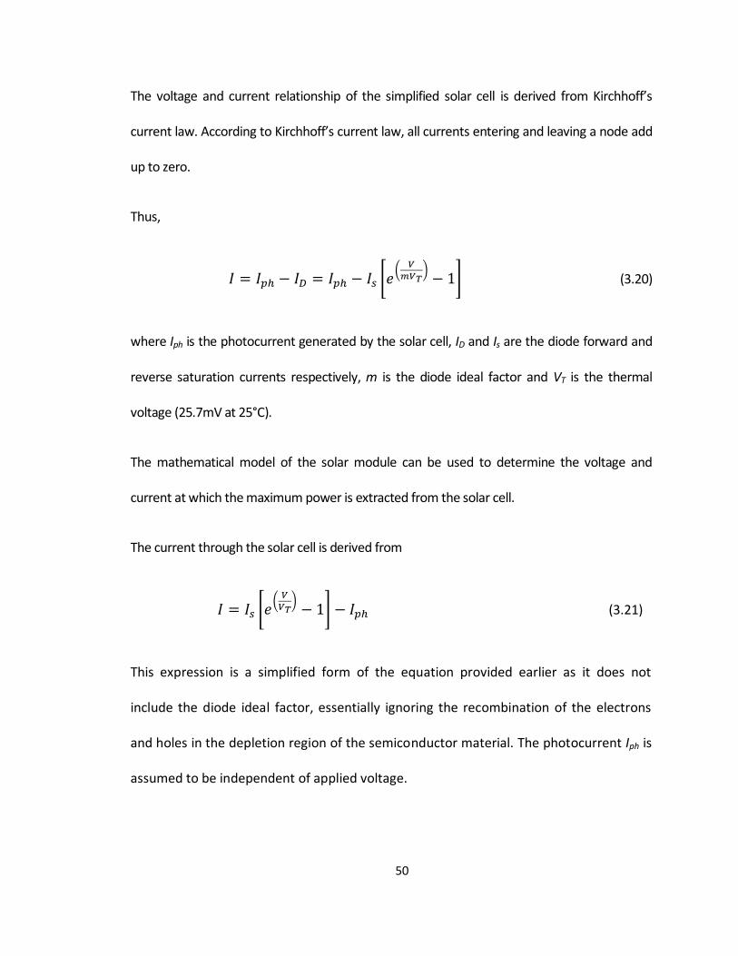
50
The voltage and current relationship of the simplified solar cell is derived from Kirchhoff’s
current law. According to Kirchhoff’s current law, all currents entering and leaving a node add
up to zero.
Thus,
(3.20)
where Iph is the photocurrent generated by the solar cell, ID and Is are the diode forward and
reverse saturation currents respectively, m is the diode ideal factor and VT is the thermal
voltage (25.7mV at 25°C).
The mathematical model of the solar module can be used to determine the voltage and
current at which the maximum power is extracted from the solar cell.
The current through the solar cell is derived from
(3.21)
This expression is a simplified form of the equation provided earlier as it does not
include the diode ideal factor, essentially ignoring the recombination of the electrons
and holes in the depletion region of the semiconductor material. The photocurrent Iph is
assumed to be independent of applied voltage.
51
The short circuit current Isc is the current with no voltage applied and equals
(3.22)
The open circuit voltage Voc is the voltage with zero current and equals
(3.23)
The total power dissipated equals
(3.24)
Considering that the maximum power occurs when
, it is possible to derive the
maximum voltage point Vm and the maximum current point Im as
(3.25)
At the maximum power point, the equation can be rewritten as
(3.26)
Vm is calculated by solving the transcendent equation above provided Voc is known. The
maximum current point Im is
(3.27)
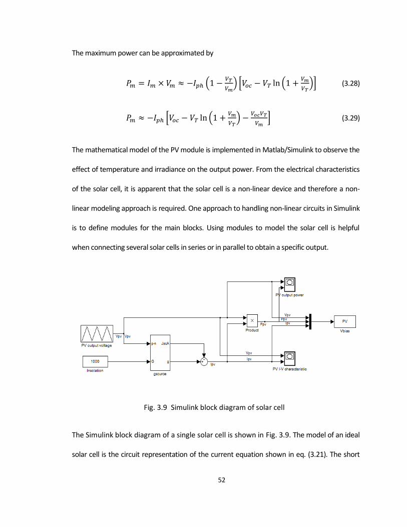
52
The maximum power can be approximated by
(3.28)
(3.29)
The mathematical model of the PV module is implemented in Matlab/Simulink to observe the
effect of temperature and irradiance on the output power. From the electrical characteristics
of the solar cell, it is apparent that the solar cell is a non-linear device and therefore a non-
linear modeling approach is required. One approach to handling non-linear circuits in Simulink
is to define modules for the main blocks. Using modules to model the solar cell is helpful
when connecting several solar cells in series or in parallel to obtain a specific output.
Fig. 3.9 Simulink block diagram of solar cell
The Simulink block diagram of a single solar cell is shown in Fig. 3.9. The model of an ideal
solar cell is the circuit representation of the current equation shown in eq. (3.21). The short
53
circuit current is proportional to the incident irradiance on the solar cell and this is
implemented in Simulink by assigning the value of the short circuit current to a voltage-
controlled current source. The voltage-controlled current source used is named ‘gsource’ and is
given by
(3.30)
where A is the solar cell surface area, Jsc is the short-circuit current density under
standard conditions (AM1.5G, 1000 W/m2, 25 ºC cell temperature), and G is the value of
the irradiance in W/m2.
The above equation gives the value of the short circuit current at any irradiance value G, so
long as the proportionality between irradiance and short circuit current holds. The solar
cell module is connected to an external measurement circuit in order to obtain the I-V
characteristic. The external circuit includes a DC bias voltage source which is swept from
0 V to 600 mV and the simulated I-V characteristic is shown in Fig. 3.10. The parameters
of the solar cell are taken from [24].
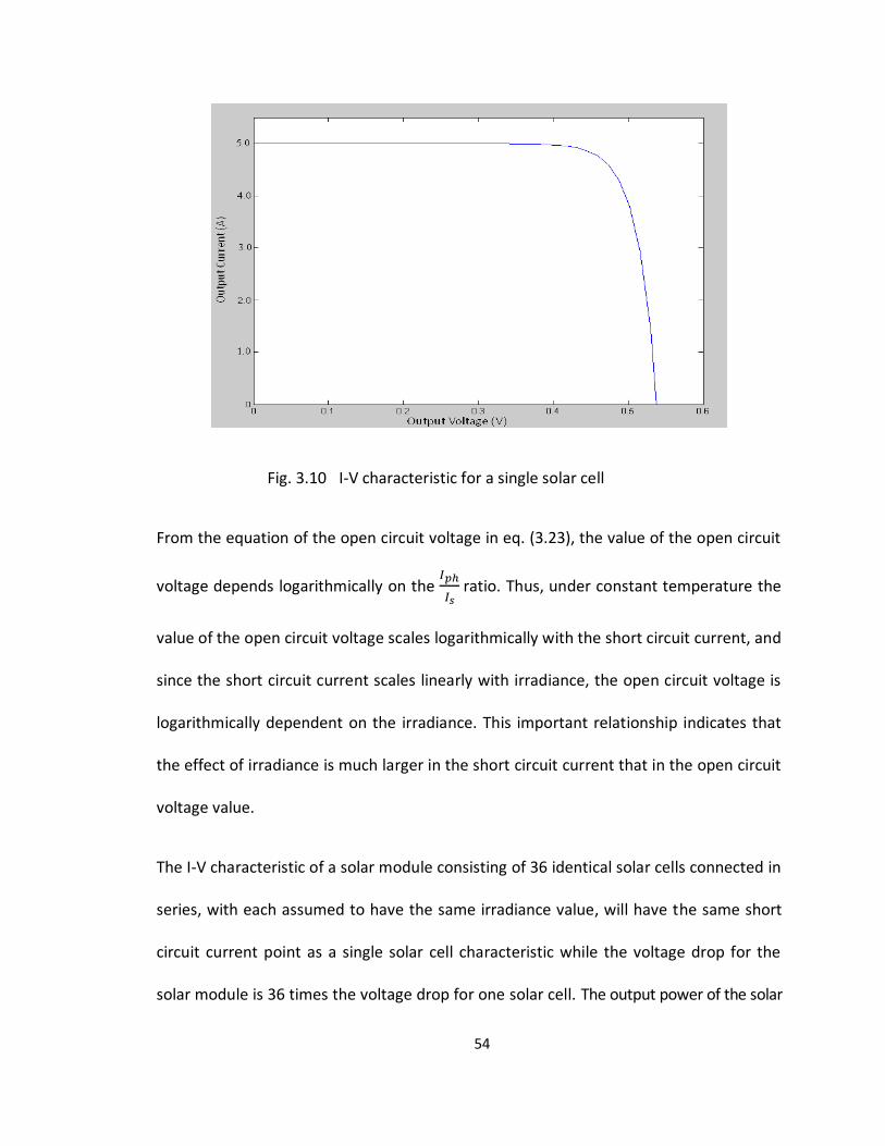
54
Fig. 3.10 I-V characteristic for a single solar cell
From the equation of the open circuit voltage in eq. (3.23), the value of the open circuit
voltage depends logarithmically on the
ratio. Thus, under constant temperature the
value of the open circuit voltage scales logarithmically with the short circuit current, and
since the short circuit current scales linearly with irradiance, the open circuit voltage is
logarithmically dependent on the irradiance. This important relationship indicates that
the effect of irradiance is much larger in the short circuit current that in the open circuit
voltage value.
The I-V characteristic of a solar module consisting of 36 identical solar cells connected in
series, with each assumed to have the same irradiance value, will have the same short
circuit current point as a single solar cell characteristic while the voltage drop for the
solar module is 36 times the voltage drop for one solar cell. The output power of the solar
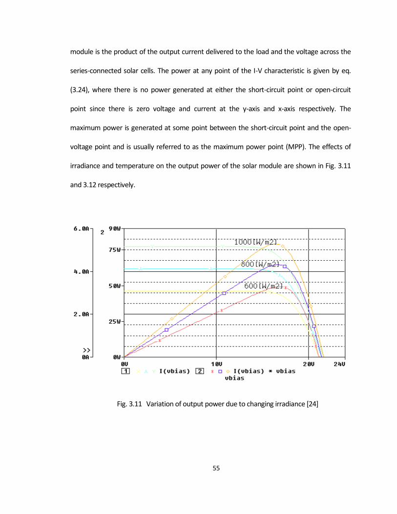
55
module is the product of the output current delivered to the load and the voltage across the
series-connected solar cells. The power at any point of the I-V characteristic is given by eq.
(3.24), where there is no power generated at either the short-circuit point or open-circuit
point since there is zero voltage and current at the y-axis and x-axis respectively. The
maximum power is generated at some point between the short-circuit point and the open-
voltage point and is usually referred to as the maximum power point (MPP). The effects of
irradiance and temperature on the output power of the solar module are shown in Fig. 3.11
and 3.12 respectively.
Fig. 3.11 Variation of output power due to changing irradiance [24]
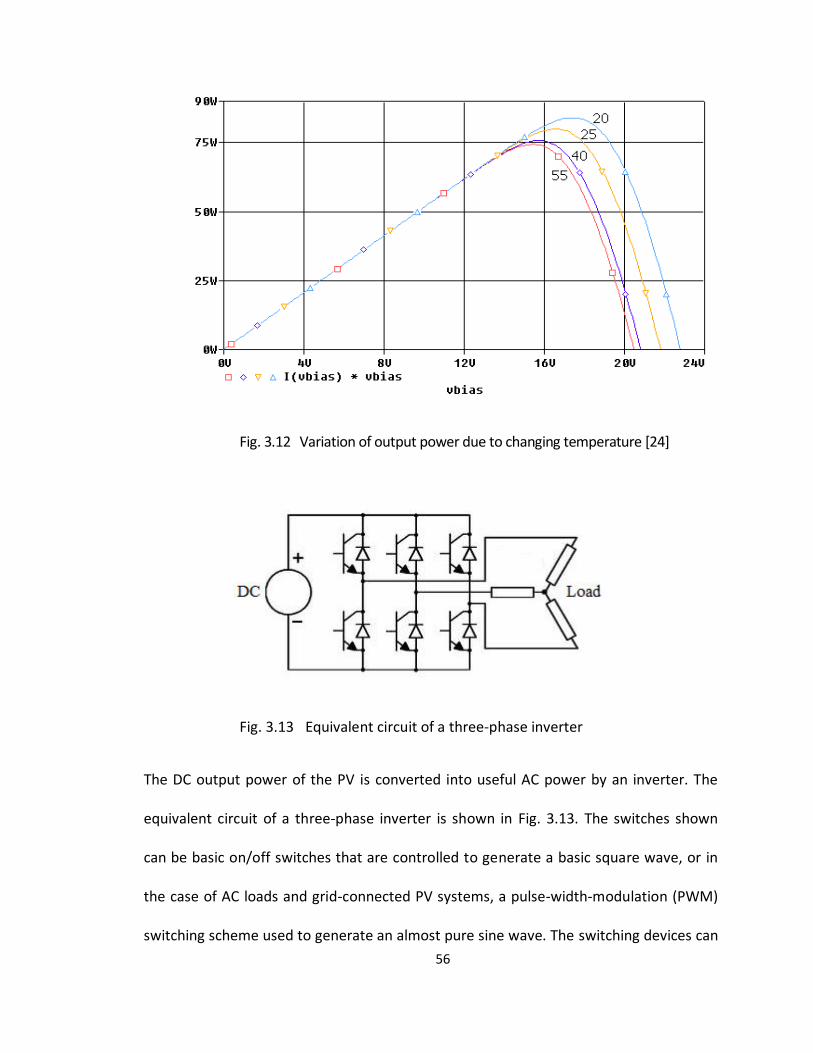
56
Fig. 3.12 Variation of output power due to changing temperature [24]
Fig. 3.13 Equivalent circuit of a three-phase inverter
The DC output power of the PV is converted into useful AC power by an inverter. The
equivalent circuit of a three-phase inverter is shown in Fig. 3.13. The switches shown
can be basic on/off switches that are controlled to generate a basic square wave, or in
the case of AC loads and grid-connected PV systems, a pulse-width-modulation (PWM)
switching scheme used to generate an almost pure sine wave. The switching devices can
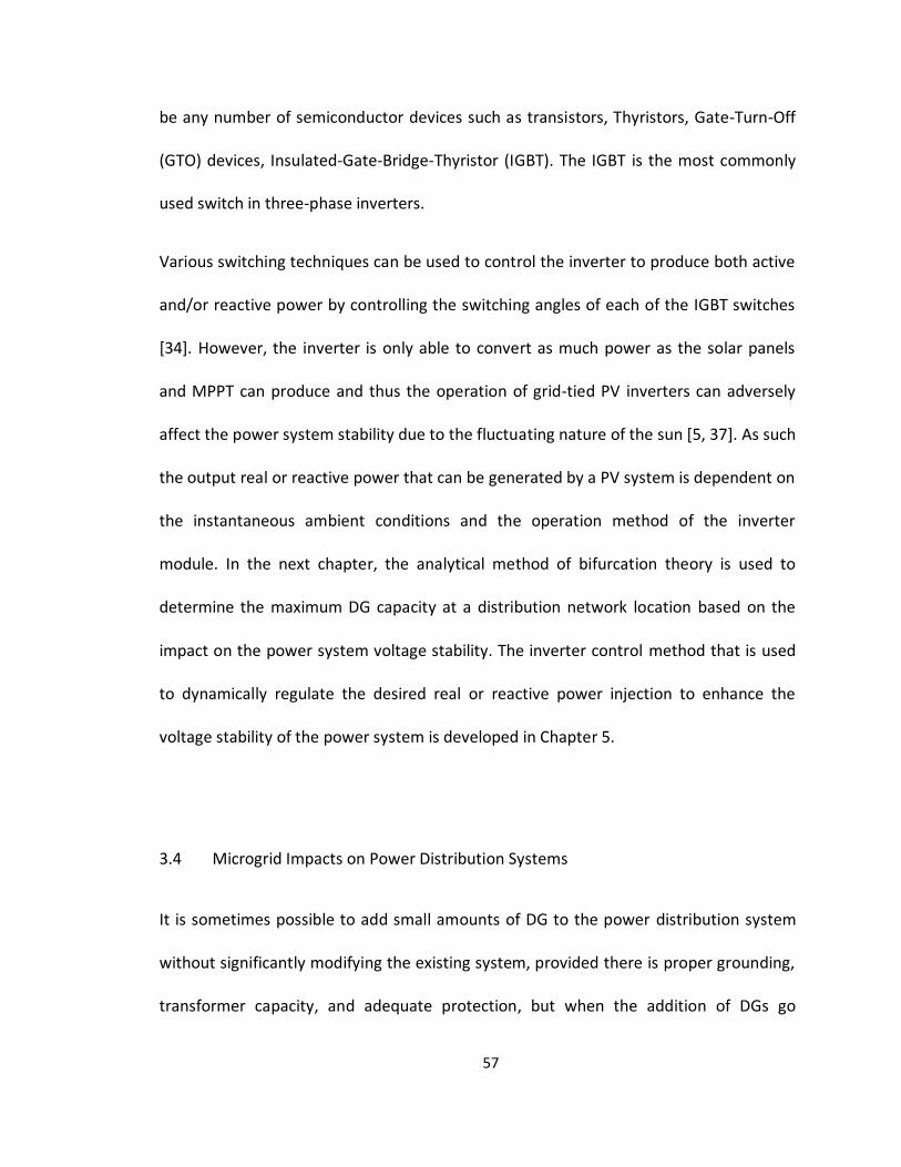
57
be any number of semiconductor devices such as transistors, Thyristors, Gate-Turn-Off
(GTO) devices, Insulated-Gate-Bridge-Thyristor (IGBT). The IGBT is the most commonly
used switch in three-phase inverters.
Various switching techniques can be used to control the inverter to produce both active
and/or reactive power by controlling the switching angles of each of the IGBT switches
[34]. However, the inverter is only able to convert as much power as the solar panels
and MPPT can produce and thus the operation of grid-tied PV inverters can adversely
affect the power system stability due to the fluctuating nature of the sun [5, 37]. As such
the output real or reactive power that can be generated by a PV system is dependent on
the instantaneous ambient conditions and the operation method of the inverter
module. In the next chapter, the analytical method of bifurcation theory is used to
determine the maximum DG capacity at a distribution network location based on the
impact on the power system voltage stability. The inverter control method that is used
to dynamically regulate the desired real or reactive power injection to enhance the
voltage stability of the power system is developed in Chapter 5.
3.4 Microgrid Impacts on Power Distribution Systems
It is sometimes possible to add small amounts of DG to the power distribution system
without significantly modifying the existing system, provided there is proper grounding,
transformer capacity, and adequate protection, but when the addition of DGs go
58
beyond the limit of what the already designed system can support, it is necessary to
modify the existing system equipment and protection to facilitate the safe integration of
new DGs [66]. The addition of new equipment may include larger switchgears,
reconfigured protection systems, improved dynamic voltage regulation systems and
revised grounding.
Some of the benefits that may be derived from addition of DGs include reduction in T&D
losses, enhanced service reliability and quality, improved voltage regulation and relieved
T&D system congestion [67]. However, interconnecting DGs to the grid could
alternatively worsen the performance of the power system leading to negative
consequences [14, 15, 17]. In fact, the reliability of the power system may be reduced if
the DG is not properly coordinated with the existing power system protection and leads
to the unnecessary tripping of protection devices or exceeding the safe operating limit
for power system equipment. The addition of DGs may also introduce voltage harmonics
and flickers due to poor voltage regulation which can seriously impact on the operation
and performance of the electric power system and lead to equipment damage at
downstream loads.
To address the challenges related to connecting DGs to the existing power system,
standards for interconnecting DGs with electric power systems were established in
2003. The IEEE 1547 (2003) interconnection standard was established to provide
interconnection technical specifications and requirements and test specifications and
requirements. Before examining the major technical and test specifications and
59
requirements , it is important to note that IEEE 1547 is limited to DGs with up to 10 MVA
aggregate DR capacity, interconnection at typical primary (~2.4 kV to 34.5 kV) or
secondary (<600V) voltage levels, with the main emphasis being on radial systems. The
interconnection technical specifications and requirements focuses on general
interconnection requirements, response to area electric power system (EPS) abnormal
conditions, power quality, and islanding phenomenon. Also, the interconnection test
specifications and requirements address design tests, production tests, interconnection
installation evaluations and commissioning tests.
Prior to deploying DGs in the field, design and production tests are required to be
carried out to determine if certain IEEE 1547 requirements have been met. The design
tests on interconnection equipment include testing the response of the equipment to
abnormal voltage and frequency, testing the interconnect integrity, detection of
harmonics, and use of active techniques to detect unintentional islanding [16]. The
installation design evaluation examines the impact on Area EPS system voltage,
grounding integration, isolation device, Area EPS fault sensing, reclosing coordination,
flicker, and passive techniques to detect unintentional islanding [16].
Although IEEE 1547 standard covers a broad range of interconnect issues, not all
technical issues are currently addressed by the standard. Some of the technical issues
that are not addressed but need to be investigated include impact on Area EPS
overcurrent protection scheme, DG penetration limits, redundancy, and dynamic
character of distribution system (loads change and frequent configuration changes).
60
During normal Area EPS operation, the DG impact of greatest concern is the voltage
regulation, as this impacts most on the stability of the overall power system [68].
Specifically, IEEE 1547 states that the DG shall not actively regulate the voltage at the
point of common coupling (PCC) nor cause the Area EPS service voltage at other local
EPS’s to go outside the requirements of ANSI (84.1-1995, Range A ) [16].
3.4.1 Islanding Phenomenon
Another technical issue of great concern resulting from one or more DGs being
connected to the power system is unintentional islanding, which occurs when a portion
of the distribution system becomes electrically isolated from the grid, yet continues to
be energized by the DG connected to the isolated subsystem. Sometimes it is desirable
to operate in an island mode, such as when DG is used as on-site backup generation, but
in general, unintentional islanding is an undesirable situation.
DG is sometimes used to provide backup power to a facility, or to supply power to
remote loads. In the former case, the DG is designed to maintain continuous power
supply to the facility when a fault occurrence leads to disconnection from the main grid.
In the latter case, the DG is designed to operate in a stand- alone mode and is used to
supply power to loads that are inaccessible to grid supply. An example of such
application is the operation of DG to power mobile telecommunications base stations in
remote regions. In the case where the DG is used to provide backup power, the DG
61
supplies the load demand until grid supply is restored. Proper safety and protection
measures must be taken to ensure that the DG is not inadvertently feeding power to the
grid, as this can pose a major safety risk. A section of the distribution network
containing a DG providing backup power may be de-energized from the grid but still
pose a safety risk to maintenance personal working in the area if the DG is of sufficient
capacity and inadvertently feeds power back into the de-energized portion of the grid.
More recently, DG microgrids are becoming more prominent where the loads are served
concurrently by the DG and the main grid.
The phenomenon where a DG inadvertently supplies power to a de-energized section of
the grid is described as unintentional islanding. The occurrence of unintentional islands
in the distribution network is one of the major issues in interconnected systems with the
rapid growth of DG deployment [69]. With an ever increasing level of DG penetration in
the distribution network, it is expected that the likelihood of unintentional islanding has
substantially increased along with the concerns associated with the phenomenon. This
is particularly the case among utilities and network operators [69, 70]. The main hazards
associated with unintentional islanding include supplying power that exceeds the
acceptable limits for voltage, frequency, flickers and other power quality parameters;
un-cleared faults due to unearthed operation leading to sustained fault currents; out-of-
phase reclosing of circuit breakers; and electric shock as a result of touching live
conductors assumed to be de-energized. Thus, unintentional islanding may cause
malfunction or damage of network and customer equipment, or in the case of electric
shock, lead to serious bodily injuries. Unintentional islanding occurs when the DG

62
interconnected to the grid does not realize loss-of-mains and continues to supply power
to the grid [70]. It is necessary to have a means of detecting when unintentional
islanding has occurred. If unintentional islanding is detected, it is necessary to
disconnect the DG in order to prevent sustained operations under the undesired
conditions.
Basically, there are two main types of anti- islanding detection methods - active anti-
islanding detection and passive anti-islanding detection techniques. An Island occurs,
and theoretically, remains undetectable if the Island’s load is constant and exactly equal
to real and reactive power output provided by the islands DG [71]. In practice, this
scenario is unrealistic as loads are not constant and exact balance between DG supply
and demand is unlikely. If there is a significant mismatch between the real and reactive
power output of the DG and the island load demand, the voltage and frequency changes
rapidly [71]. The island operation is terminated when the voltage and/or frequency
reach preset under/over-voltage or frequency trip points. In general, the greater the
difference between the DG supply and island load, the quicker the voltage or frequency
deviation approaches the trip point [72]. Other characteristics that determine the time
required to reach the trip point include the DG control characteristics, the voltage
demand characteristics of the island’s loads, and the mechanical inertia of the loads.
When the DG is equipped with under and over-voltage and frequency relays, it is
considered to employ basic passive anti-islanding techniques.
63
When it is not sufficient to base island detection on the imbalance between DG supply
and island load demand, for example, in cases where the DG supply roughly matches
load demand, then active anti-islanding methods are required. Active anti-islanding
techniques have been developed to accelerate the resulting frequency and voltage
deviations, such that the trip points are reached more rapidly [71, 72]. These active anti-
islanding techniques modulate the real and reactive power output of the DG in response
to changes in frequency and voltage magnitude. Active anti-islanding employing these
techniques use positive feedback destabilizing control, where any randomly occurring
changes in voltage or frequency is amplified. Under normal operating conditions, when
the DG is interconnected with the grid, the output of the DG is small relative to the grid,
and the invariance of the grid voltage and frequency will maintain stability. Once the
grid is disconnected (loss-of-mains), the active anti-islanding makes the island inherently
unstable and the DG is driven to the trip point.
3.4.2 Interconnection at the Point-of-Common Coupling
Voltage sags or momentary reductions in the rms voltage magnitude lasting between
half a cycle and several seconds are usually caused by fault conditions on the power
distribution system [73]. The starting of induction motors can also cause voltage sags on
the power system although the effect of motor starts by itself should not pose any
significant problems on a properly designed system. However, the combination of a
fault condition on the system with the effect of motors starting or restarting can

64
significantly impact on the voltage stability of the power distribution system [74]. It is
useful to briefly examine the dominant types of fault in terms of their magnitudes and
durations.
A power system can either experience a short circuit fault or an open circuit fault. The
short circuit fault occurs when a low impedance path is formed between phases or
between a phase or phases and ground. This may result from insulation failure causing
the current carrying conductor to be exposed to ground or other conductors. The low
impedance path causes very high currents to flow which affects the voltage magnitude
and may damage equipment. There are four different types of short-circuit faults that
can occur on a three-phase system – three-phase, line-to-line, line-to-ground, and the
double line-to-ground faults. Only the three-phase fault shown in Fig. 3.14 produces
balanced voltages and currents. Open circuit faults typically result from fuse operation
in one or more phases of a fuse-protected three-phase circuit. In this case, part of the
system continues to operate in an unbalanced manner.
The primary reason to determine fault magnitudes and duration is to size protective
devices; therefore it is only necessary to consider the fault type that produces the
largest fault current, i.e. the worst case scenario. In most cases, the worst case is the
three-phase fault [75], and as such, the three phase fault will be primarily considered in
this work. It is important to point out that while the three-phase fault is often the most
severe case, this assumption does not always apply [75, 76]. For power system planning
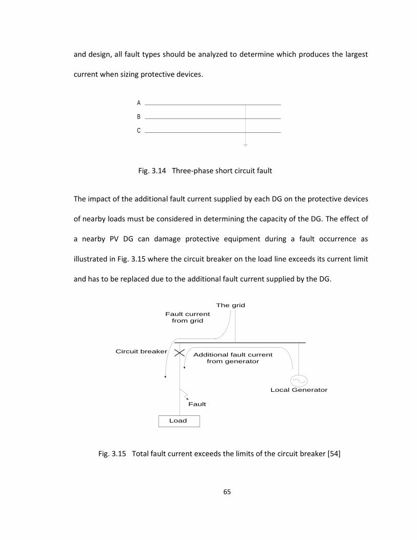
65
and design, all fault types should be analyzed to determine which produces the largest
current when sizing protective devices.
A
B
C
Fig. 3.14 Three-phase short circuit fault
The impact of the additional fault current supplied by each DG on the protective devices
of nearby loads must be considered in determining the capacity of the DG. The effect of
a nearby PV DG can damage protective equipment during a fault occurrence as
illustrated in Fig. 3.15 where the circuit breaker on the load line exceeds its current limit
and has to be replaced due to the additional fault current supplied by the DG.
Load
Fault
The grid
Local Generator
Circuit breaker
Fault current
from grid
Additional fault current
from generator
Fig. 3.15 Total fault current exceeds the limits of the circuit breaker [54]
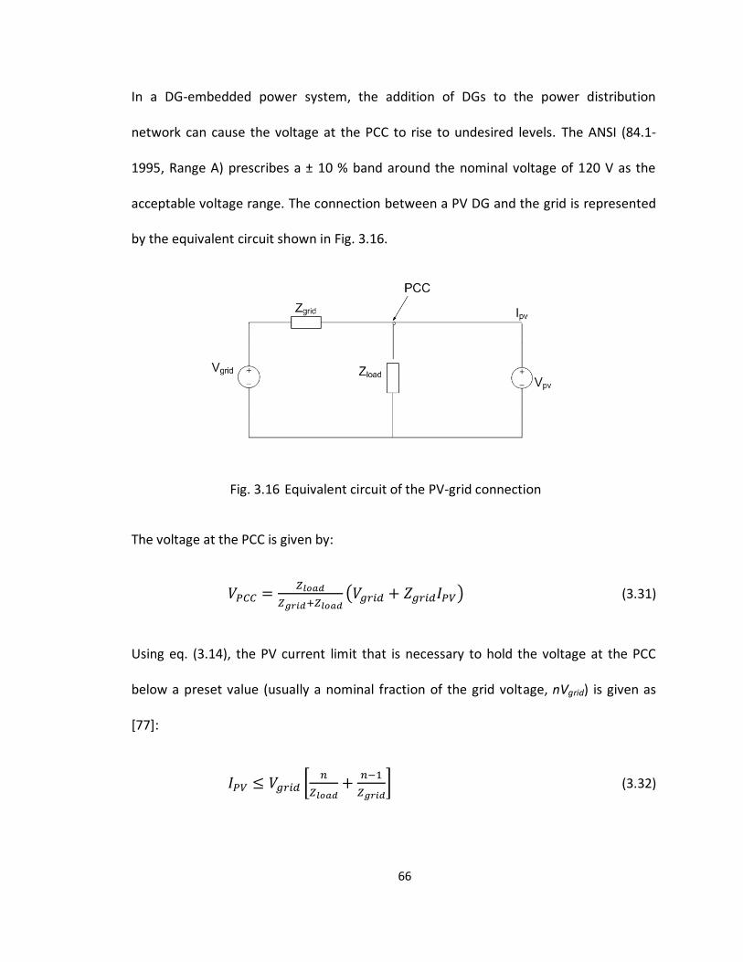
66
In a DG-embedded power system, the addition of DGs to the power distribution
network can cause the voltage at the PCC to rise to undesired levels. The ANSI (84.1-
1995, Range A) prescribes a ± 10 % band around the nominal voltage of 120 V as the
acceptable voltage range. The connection between a PV DG and the grid is represented
by the equivalent circuit shown in Fig. 3.16.
Fig. 3.16 Equivalent circuit of the PV-grid connection
The voltage at the PCC is given by:
(3.31)
Using eq. (3.14), the PV current limit that is necessary to hold the voltage at the PCC
below a preset value (usually a nominal fraction of the grid voltage, nVgrid) is given as
[77]:
(3.32)
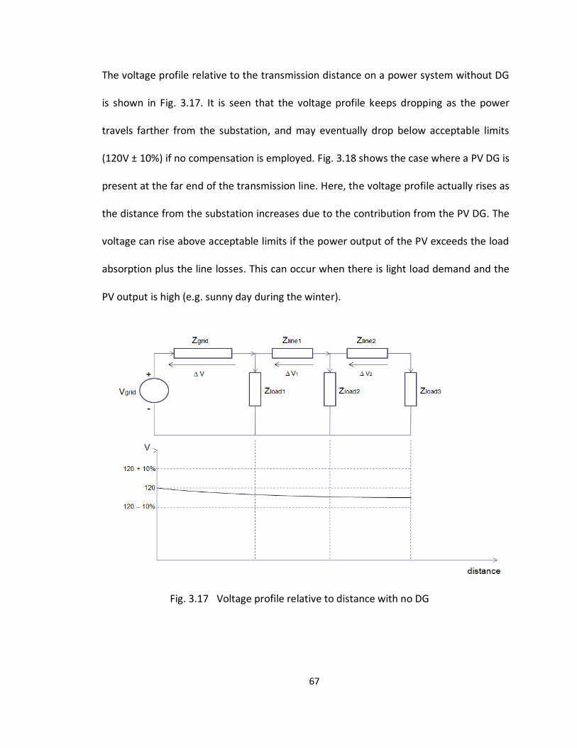
67
The voltage profile relative to the transmission distance on a power system without DG
is shown in Fig. 3.17. It is seen that the voltage profile keeps dropping as the power
travels farther from the substation, and may eventually drop below acceptable limits
(120V ± 10%) if no compensation is employed. Fig. 3.18 shows the case where a PV DG is
present at the far end of the transmission line. Here, the voltage profile actually rises as
the distance from the substation increases due to the contribution from the PV DG. The
voltage can rise above acceptable limits if the power output of the PV exceeds the load
absorption plus the line losses. This can occur when there is light load demand and the
PV output is high (e.g. sunny day during the winter).
Fig. 3.17 Voltage profile relative to distance with no DG
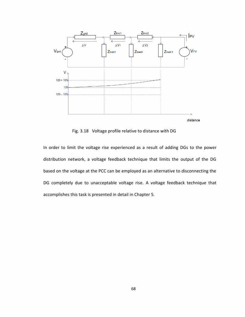
68
Fig. 3.18 Voltage profile relative to distance with DG
In order to limit the voltage rise experienced as a result of adding DGs to the power
distribution network, a voltage feedback technique that limits the output of the DG
based on the voltage at the PCC can be employed as an alternative to disconnecting the
DG completely due to unacceptable voltage rise. A voltage feedback technique that
accomplishes this task is presented in detail in Chapter 5.
69
4. ANALYTICAL APPROACH TO VOLTAGE INSTABILITY
The source side of the power system stability dynamic has been examined in the
previous chapter, but it is well known that loads are the main driver of voltage
instability. Induction motors are the typical loads found in the industrial sector, and the
impact of these motor loads on the power system stability is investigated in this
chapter. The voltage-power characteristic of induction motor loads is used to define the
loadability limit for an industrial power system and bifurcation theory is applied to
determine the short-term and long-term margins to voltage instability. Bifurcation
theory deals with the emergence of sudden changes in system response due to smooth
variations in system parameters - an effect which is similar to voltage instability or
collapse. The system components are implemented in Matlab and the voltage stability
scenarios are investigated for both the short-term and long-term cases.
4.1 Voltage Instability Mechanism
Voltage instability occurs when the power system is unable to maintain steady voltages
at all buses. This stems from the attempt of load dynamics to restore power
consumption beyond the capability of the power system [54]. A power system subjected
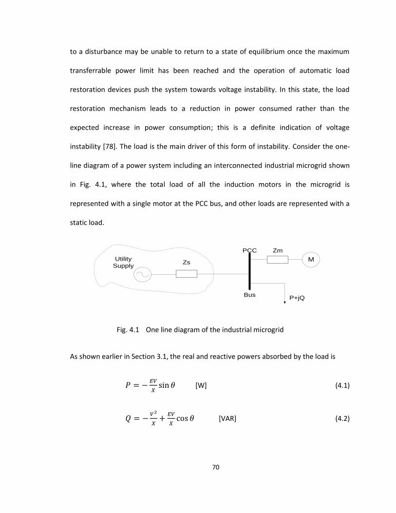
70
to a disturbance may be unable to return to a state of equilibrium once the maximum
transferrable power limit has been reached and the operation of automatic load
restoration devices push the system towards voltage instability. In this state, the load
restoration mechanism leads to a reduction in power consumed rather than the
expected increase in power consumption; this is a definite indication of voltage
instability [78]. The load is the main driver of this form of instability. Consider the one-
line diagram of a power system including an interconnected industrial microgrid shown
in Fig. 4.1, where the total load of all the induction motors in the microgrid is
represented with a single motor at the PCC bus, and other loads are represented with a
static load.
ZsM
Zm
P+jQ
PCC
Bus
Utility
Supply
Fig. 4.1 One line diagram of the industrial microgrid
As shown earlier in Section 3.1, the real and reactive powers absorbed by the load is
[W] (4.1)
[VAR] (4.2)
71
Eqs. (4.1) and (4.2) represent the load flow equations of the simplified microgrid shown
in Fig. 4.1 where X is the Thevenin equivalent impedance. Solving the load flow
equations for the condition to have at least one solution results in [54]:
(4.3)
The maximum power transfer limits for the real and reactive powers can be determined
by setting Q and P to zero in eq. (4.3) respectively,
For Q = 0,
(4.4)
For P = 0,
(4.5)
where
is equal to the short-circuit power at the load.
From eqs. (4.4) and (4.5) above, the maximum real power that can be consumed at the
load is half the short-circuit power while the maximum reactive power that can be
consumed is a fourth of the short-circuit power. Therefore, for a system operating at or
near peak load conditions, a sudden rise in reactive power demand (e.g. due to voltage
sag) is accompanied by an increase in the real power consumption. Under the stressed
conditions of peak load demand, there is usually insufficient power transfer capability
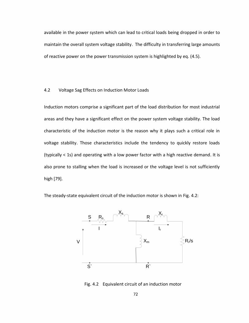
72
available in the power system which can lead to critical loads being dropped in order to
maintain the overall system voltage stability. The difficulty in transferring large amounts
of reactive power on the power transmission system is highlighted by eq. (4.5).
4.2 Voltage Sag Effects on Induction Motor Loads
Induction motors comprise a significant part of the load distribution for most industrial
areas and they have a significant effect on the power system voltage stability. The load
characteristic of the induction motor is the reason why it plays such a critical role in
voltage stability. Those characteristics include the tendency to quickly restore loads
(typically < 1s) and operating with a low power factor with a high reactive demand. It is
also prone to stalling when the load is increased or the voltage level is not sufficiently
high [79].
The steady-state equivalent circuit of the induction motor is shown in Fig. 4.2:
Rs
Xs
Rr/sXm
Xr
I Ir
V
· ·
· ·
S
S` R`
R
Fig. 4.2 Equivalent circuit of an induction motor
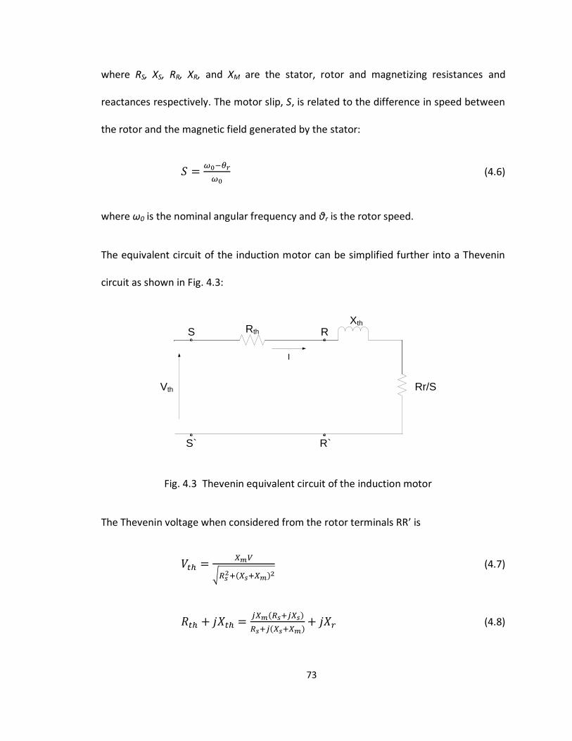
73
where RS, XS, RR, XR, and XM are the stator, rotor and magnetizing resistances and
reactances respectively. The motor slip, S, is related to the difference in speed between
the rotor and the magnetic field generated by the stator:
(4.6)
where ω0 is the nominal angular frequency and θr is the rotor speed.
The equivalent circuit of the induction motor can be simplified further into a Thevenin
circuit as shown in Fig. 4.3:
Rth
Xth
I
Vth
· ·
· ·
S
S` R`
R
Rr/S
Fig. 4.3 Thevenin equivalent circuit of the induction motor
The Thevenin voltage when considered from the rotor terminals RR’ is
(4.7)
(4.8)
74
The current drawn by the motor in terms of the stator and electrical impedances when
considered from the stator terminals SS’ is
(4.9)
where,
(4.10)
The rotor and stator in an induction machine are separated by an air-gap that allows the
free rotation of the rotor. The air-gap power, Pg, depends on the motor parameters and
the slip for any given terminal voltage. The per unit air-gap power is equal to the
developed electrical torque, Te, of the motor.
The air-gap power in the induction motor is equal to the power absorbed by the
resistance
and can be expressed as [80]:
(4.11)
The electrical torque developed in the Thevenin equivalent circuit is given as a function
of the voltage Vth and slip by
(4.12)
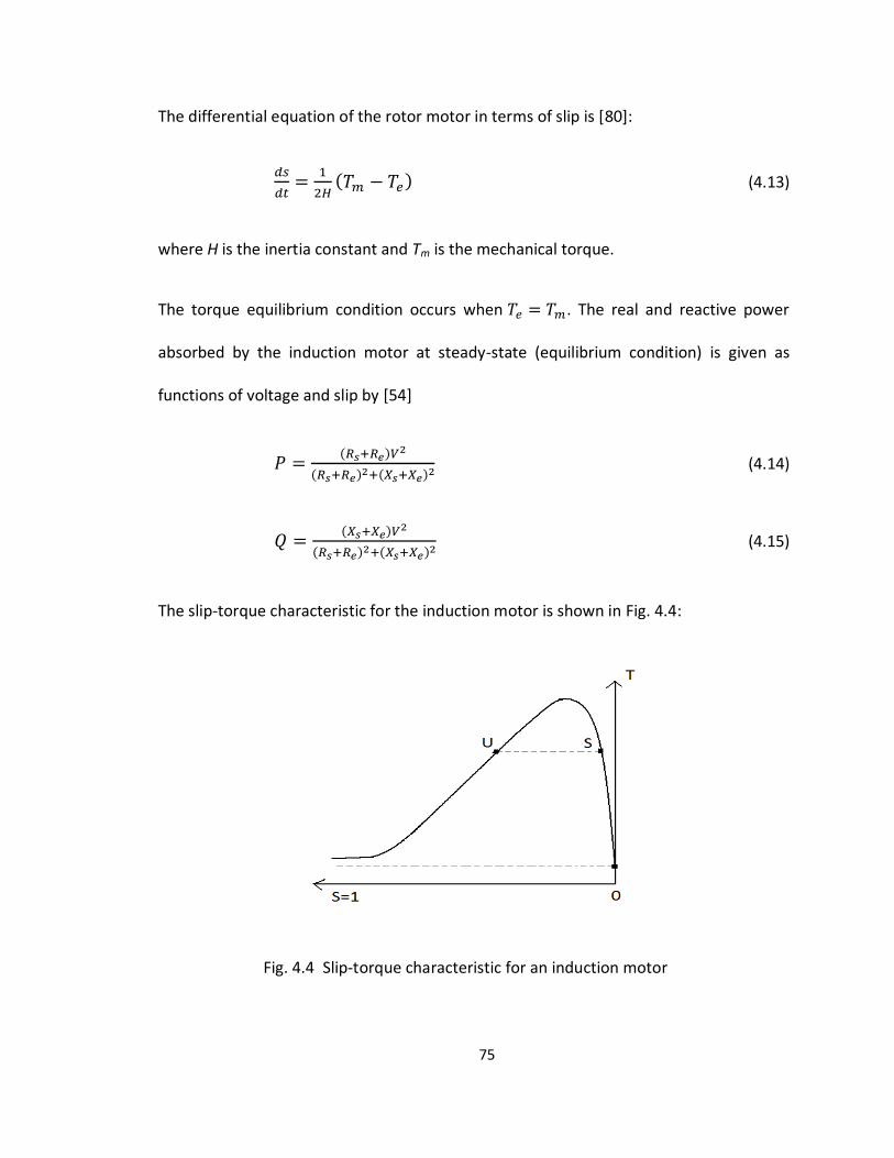
75
The differential equation of the rotor motor in terms of slip is [80]:
(4.13)
where H is the inertia constant and Tm is the mechanical torque.
The torque equilibrium condition occurs when . The real and reactive power
absorbed by the induction motor at steady-state (equilibrium condition) is given as
functions of voltage and slip by [54]
(4.14)
(4.15)
The slip-torque characteristic for the induction motor is shown in Fig. 4.4:
Fig. 4.4 Slip-torque characteristic for an induction motor

76
The three types of induction motor models - the constant torque model, the quadratic
torque model, and the composite torque model – that are typically found in the
industrial sector and exhibit different steady-state behaviors under different torques are
used in this study and are briefly presented next. Some industrial motors exhibit the
constant torque characteristic although the majority of industrial motors are more
closely represented by the quadratic and composite torque models [81, 82].
In the constant torque model, the mechanical torque is parallel to the s-axis. The motor
stalls when the mechanical torque exceeds the maximum available electrical torque. PV
and QV curves can be used to express the relationship between the consumed power
and the terminal voltage and they are typically used to assess the voltage stability of
power systems. The constant mechanical torque is given as [82]:
(4.16)
The PV and QV curves for a constant torque model using eqs. (4.1) and (4.2) are shown
in Fig. 4.5.
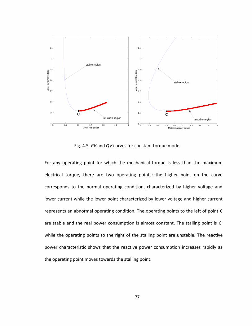
77
Fig. 4.5 PV and QV curves for constant torque model
For any operating point for which the mechanical torque is less than the maximum
electrical torque, there are two operating points: the higher point on the curve
corresponds to the normal operating condition, characterized by higher voltage and
lower current while the lower point characterized by lower voltage and higher current
represents an abnormal operating condition. The operating points to the left of point C
are stable and the real power consumption is almost constant. The stalling point is C,
while the operating points to the right of the stalling point are unstable. The reactive
power characteristic shows that the reactive power consumption increases rapidly as
the operating point moves towards the stalling point.
0.4 0.5 0.6 0.7 0.8 0.9 10.4
0.5
0.6
0.7
0.8
0.9
1
1.1
Motor real power
Mo
tor
term
ina
l vo
ltag
e
0.2 0.3 0.4 0.5 0.6 0.7 0.8 0.9 1 1.10.4
0.5
0.6
0.7
0.8
0.9
1
1.1
Motor imaginary power
Mo
tor
term
ina
l vo
ltag
e
unstable region
stable region
unstable region
stable region
CC
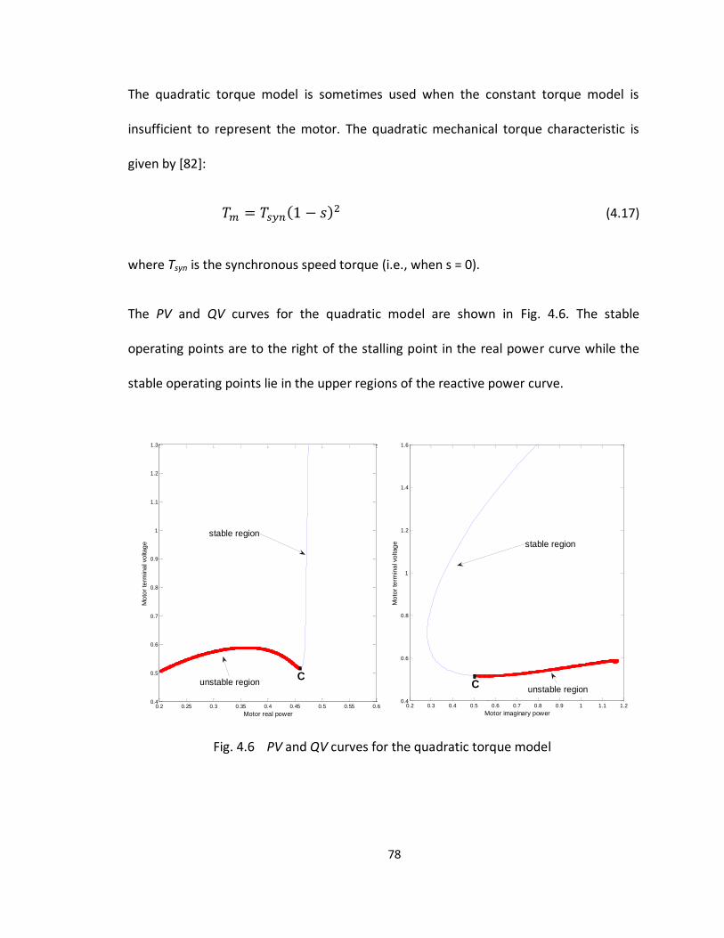
78
The quadratic torque model is sometimes used when the constant torque model is
insufficient to represent the motor. The quadratic mechanical torque characteristic is
given by [82]:
(4.17)
where Tsyn is the synchronous speed torque (i.e., when s = 0).
The PV and QV curves for the quadratic model are shown in Fig. 4.6. The stable
operating points are to the right of the stalling point in the real power curve while the
stable operating points lie in the upper regions of the reactive power curve.
Fig. 4.6 PV and QV curves for the quadratic torque model
0.2 0.25 0.3 0.35 0.4 0.45 0.5 0.55 0.60.4
0.5
0.6
0.7
0.8
0.9
1
1.1
1.2
1.3
Motor real power
Mo
tor
term
ina
l vo
ltag
e
0.2 0.3 0.4 0.5 0.6 0.7 0.8 0.9 1 1.1 1.20.4
0.6
0.8
1
1.2
1.4
1.6
Motor imaginary power
Mo
tor
term
ina
l vo
ltag
e
CC
stable region
stable region
unstable regionunstable region
79
The composite torque model is a combination of the constant torque model and the
quadratic model. It takes into account the static torque due to friction. The composite
torque characteristic is given by [82]:
(4.18)
where Ts is the static torque.
The composite torque model is useful when the combination of the various motor loads
exhibit different characteristics. A single induction load model can be used to represent
the cumulative effect of all the motors in an industrial facility, which may include several
tens or even hundreds of small, medium, and large sized motors that exhibit similar
characteristics. The cumulative load characteristic is the expression of the active and
reactive powers of all the loads as a function of voltage and load demand. The
exponential load model is given as [54]:
(4.19)
(4.20)
where and is the real and reactive consumed power respectively at the nominal
voltage , while and are the load power sensitivities to voltage, and c is the
cumulative load demand.
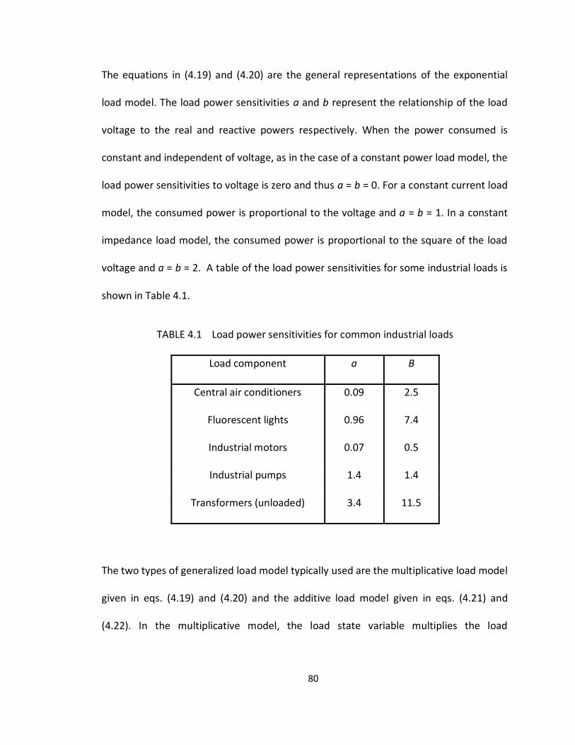
80
The equations in (4.19) and (4.20) are the general representations of the exponential
load model. The load power sensitivities a and b represent the relationship of the load
voltage to the real and reactive powers respectively. When the power consumed is
constant and independent of voltage, as in the case of a constant power load model, the
load power sensitivities to voltage is zero and thus a = b = 0. For a constant current load
model, the consumed power is proportional to the voltage and a = b = 1. In a constant
impedance load model, the consumed power is proportional to the square of the load
voltage and a = b = 2. A table of the load power sensitivities for some industrial loads is
shown in Table 4.1.
TABLE 4.1 Load power sensitivities for common industrial loads
Load component a B
Central air conditioners 0.09 2.5
Fluorescent lights 0.96 7.4
Industrial motors 0.07 0.5
Industrial pumps 1.4 1.4
Transformers (unloaded) 3.4 11.5
The two types of generalized load model typically used are the multiplicative load model
given in eqs. (4.19) and (4.20) and the additive load model given in eqs. (4.21) and
(4.22). In the multiplicative model, the load state variable multiplies the load
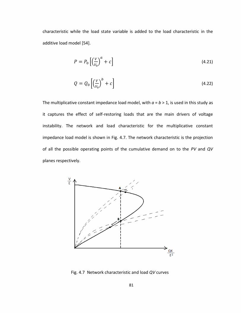
81
characteristic while the load state variable is added to the load characteristic in the
additive load model [54].
(4.21)
(4.22)
The multiplicative constant impedance load model, with a = b > 1, is used in this study as
it captures the effect of self-restoring loads that are the main drivers of voltage
instability. The network and load characteristic for the multiplicative constant
impedance load model is shown in Fig. 4.7. The network characteristic is the projection
of all the possible operating points of the cumulative demand on to the PV and QV
planes respectively.
Fig. 4.7 Network characteristic and load QV curves
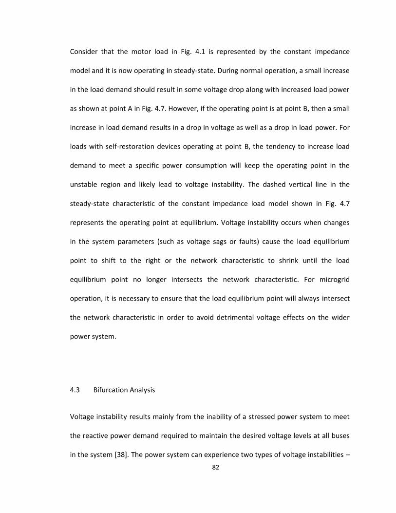
82
Consider that the motor load in Fig. 4.1 is represented by the constant impedance
model and it is now operating in steady-state. During normal operation, a small increase
in the load demand should result in some voltage drop along with increased load power
as shown at point A in Fig. 4.7. However, if the operating point is at point B, then a small
increase in load demand results in a drop in voltage as well as a drop in load power. For
loads with self-restoration devices operating at point B, the tendency to increase load
demand to meet a specific power consumption will keep the operating point in the
unstable region and likely lead to voltage instability. The dashed vertical line in the
steady-state characteristic of the constant impedance load model shown in Fig. 4.7
represents the operating point at equilibrium. Voltage instability occurs when changes
in the system parameters (such as voltage sags or faults) cause the load equilibrium
point to shift to the right or the network characteristic to shrink until the load
equilibrium point no longer intersects the network characteristic. For microgrid
operation, it is necessary to ensure that the load equilibrium point will always intersect
the network characteristic in order to avoid detrimental voltage effects on the wider
power system.
4.3 Bifurcation Analysis
Voltage instability results mainly from the inability of a stressed power system to meet
the reactive power demand required to maintain the desired voltage levels at all buses
in the system [38]. The power system can experience two types of voltage instabilities –
83
voltage collapse and unstable voltage oscillation. The power system experiences voltage
collapse if it is unable to maintain acceptable steady-state voltages after a disturbance
event [37]. Unstable voltage oscillation usually results from the interaction of controllers
with power system equipment.
Voltage instability occurs on multiple timescales, and can be classified into short-term
and long-term instabilities. Short-term voltage stability refers to the small-signal and
transient stabilities, including the stability of the dynamics of induction motors and
controllers. Long-term voltage stability refers to the long-term dynamics, including
dynamic stabilities due to generator excitation limit and load increase.
The dynamics and changes in operating condition of the power system can be
represented by differential and algebraic equations respectively. The dynamics that
result due to changes in operating condition can be decomposed into slow and fast
dynamics based on the time-scale of interest. The corresponding state variables can
similarly be decomposed into slow and fast variables [83].
Any power system can be described by the set of differential-algebraic equations (DAE)
shown in eqs. (4.23) and (4.24).
(4.23)
(4.24)
84
The differential equation in eq. (4.23) can be decomposed to separate the slow state
variables Xs from the fast state variables Xf, resulting in eqs. (4.25) and (4.26)
respectively.
(4.25)
(4.26)
where α is generally a very small number.
When α approaches zero, the differential equation of the fast state vector in eq. (4.26)
can be approximated by the algebraic equation shown in eq. (4.27). In this case, eqs.
(4.28) and (4.29) complete the approximation of the power system described by eqs.
(4.23) and (4.24).
(4.27)
(4.28)
(4.29)
The non-linear nature of power system means that non-linear analysis techniques such
as bifurcation analysis are required for power system voltage stability studies.
Bifurcation theory deals with the emergence of sudden changes in system response due
to the slow variation of smooth continuous system parameters [84]. With timescale
decomposition applied to the power system to separate slow and fast variables,
85
bifurcation analysis describes the qualitative changes of stability with smooth parameter
variations [83].
Using timescale decomposition, the DAE of the power system can be represented by
eqs. (4.27 – 4.29). If the slow variables Xs are considered as parameters, the power
system voltage stability analysis can be performed using the system dynamics
represented by the set of parameter dependent DAE shown in eqs. (4.30) and (4.31)
[83].
(4.30)
(4.31)
where x is a vector of state variables, y is a vector of algebraic variables, and p is a
vector of parameters.
Solving the DAE shown in eqs. (4.30) and (4.31) for a power system is non-trivial. In
order to simplify the analysis, the algebraic vector y can be eliminated from eq. (4.30) by
solving for y in terms of the state vector x and parameter vector p in eq. (4.31) which
results in the reduced differential equation below:
(4.32)
The equilibrium points for a system described by eqs. (4.30) and (4.31) are given as
(4.33)
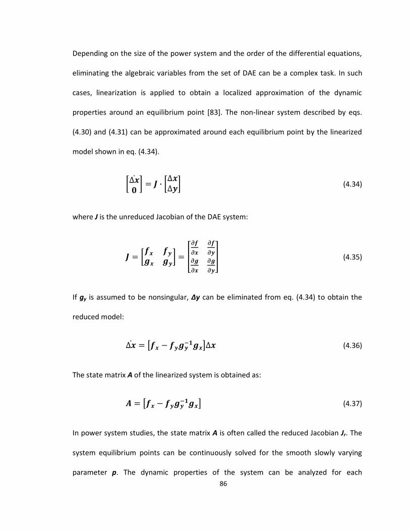
86
Depending on the size of the power system and the order of the differential equations,
eliminating the algebraic variables from the set of DAE can be a complex task. In such
cases, linearization is applied to obtain a localized approximation of the dynamic
properties around an equilibrium point [83]. The non-linear system described by eqs.
(4.30) and (4.31) can be approximated around each equilibrium point by the linearized
model shown in eq. (4.34).
(4.34)
where J is the unreduced Jacobian of the DAE system:
(4.35)
If gy is assumed to be nonsingular, ∆y can be eliminated from eq. (4.34) to obtain the
reduced model:
(4.36)
The state matrix A of the linearized system is obtained as:
(4.37)
In power system studies, the state matrix A is often called the reduced Jacobian Jr. The
system equilibrium points can be continuously solved for the smooth slowly varying
parameter p. The dynamic properties of the system can be analyzed for each
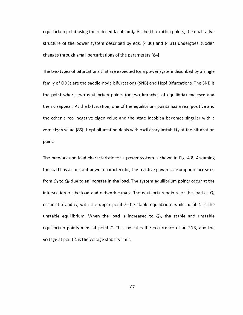
87
equilibrium point using the reduced Jacobian Jr. At the bifurcation points, the qualitative
structure of the power system described by eqs. (4.30) and (4.31) undergoes sudden
changes through small perturbations of the parameters [84].
The two types of bifurcations that are expected for a power system described by a single
family of ODEs are the saddle-node bifurcations (SNB) and Hopf Bifurcations. The SNB is
the point where two equilibrium points (or two branches of equilibria) coalesce and
then disappear. At the bifurcation, one of the equilibrium points has a real positive and
the other a real negative eigen value and the state Jacobian becomes singular with a
zero eigen value [85]. Hopf bifurcation deals with oscillatory instability at the bifurcation
point.
The network and load characteristic for a power system is shown in Fig. 4.8. Assuming
the load has a constant power characteristic, the reactive power consumption increases
from Q1 to Q2 due to an increase in the load. The system equilibrium points occur at the
intersection of the load and network curves. The equilibrium points for the load at Q1
occur at S and U, with the upper point S the stable equilibrium while point U is the
unstable equilibrium. When the load is increased to Q2, the stable and unstable
equilibrium points meet at point C. This indicates the occurrence of an SNB, and the
voltage at point C is the voltage stability limit.
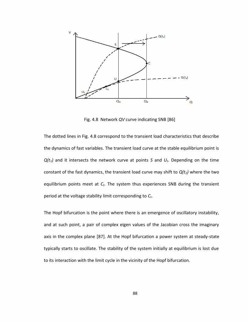
88
Fig. 4.8 Network QV curve indicating SNB [86]
The dotted lines in Fig. 4.8 correspond to the transient load characteristics that describe
the dynamics of fast variables. The transient load curve at the stable equilibrium point is
Q(t1) and it intersects the network curve at points S and Ut. Depending on the time
constant of the fast dynamics, the transient load curve may shift to Q(t2) where the two
equilibrium points meet at Ct. The system thus experiences SNB during the transient
period at the voltage stability limit corresponding to Ct.
The Hopf bifurcation is the point where there is an emergence of oscillatory instability,
and at such point, a pair of complex eigen values of the Jacobian cross the imaginary
axis in the complex plane [87]. At the Hopf bifurcation a power system at steady-state
typically starts to oscillate. The stability of the system initially at equilibrium is lost due
to its interaction with the limit cycle in the vicinity of the Hopf bifurcation.
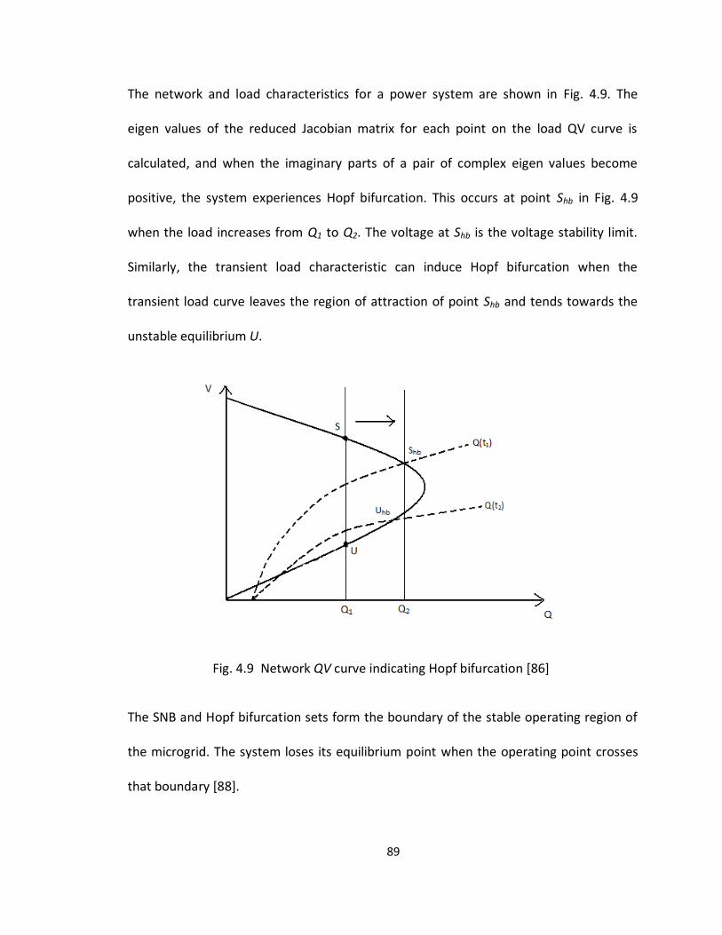
89
The network and load characteristics for a power system are shown in Fig. 4.9. The
eigen values of the reduced Jacobian matrix for each point on the load QV curve is
calculated, and when the imaginary parts of a pair of complex eigen values become
positive, the system experiences Hopf bifurcation. This occurs at point Shb in Fig. 4.9
when the load increases from Q1 to Q2. The voltage at Shb is the voltage stability limit.
Similarly, the transient load characteristic can induce Hopf bifurcation when the
transient load curve leaves the region of attraction of point Shb and tends towards the
unstable equilibrium U.
Fig. 4.9 Network QV curve indicating Hopf bifurcation [86]
The SNB and Hopf bifurcation sets form the boundary of the stable operating region of
the microgrid. The system loses its equilibrium point when the operating point crosses
that boundary [88].
90
The DAE model of the power system is used to describe the dynamics of the power
system for voltage stability analysis.
(4.38)
(4.39)
where x is the vector of dynamic state variables that typically describe time-dependent
generator voltages and p is the vector of parameters that define a specific system
configuration and operating condition.
For every value of p, the system equilibrium points are given by the solution of eq.
(4.39). The algebraic equations in eq. 4.39 are the power flow equations representing
the real and reactive power balances at the load buses, and it defines an equilibrium
manifold in the state and parameter dimensional space [88]. Bifurcation may occur at
any point along the path of the smooth parameter variations. Bifurcation occurs at the
loadability limit of a power system resulting in voltage instability.
Loads are the main driver of voltage instability and the loadability limit for a power
system is defined as the point where the load characteristic becomes tangent to the
network characteristic. Bifurcation analysis can be applied to determine the loadability
limit induced bifurcation of a microgrid, provided the load and network models are fairly
well described. For the generalized exponential load model, the consumed real and
reactive powers that define the load characteristic are [54]:
91
(4.40)
(4.41)
Dividing the power equation by V to get the load current results in
(4.42)
(4.43)
Solving eqs. (4.42) and (4.43) results in a single solution V for every value of the
cumulative load c, and therefore there is no loadability limit resulting from the
bifurcation of the load operating point for a microgrid consisting of mainly exponential-
type loads (a = b > 1). Instead the loadability limit for such microgrid is bounded by the
permissible voltage rise (or drop) at the PCC bus. In the case where the loads are less
sensitive to voltage than constant current (a = b < 1), there is a maximum value of c that
corresponds to the maximum loadability, cm, where there are two solutions for c < cm
and no solutions for c > cm.
For a power system described by
(4.44)

92
where corresponds to the steady-state network equations when both the short-term
and long-term dynamics are considered constant and c corresponds to the load
demand.
The Jacobian of the steady-state equations is singular at the loadability limit, Lm.
det = 0 (4.45)
The steady-state equations from eqs. (4.40) and (4.41) for the exponential load model
are given in terms of the load current as
When the nominal operating voltage is assumed to be 1 p.u., i.e. V0 = 1 p.u., the
Jacobian of the system is
(4.46)
The corresponding singularity condition of is
(4.47)
or
(4.48)
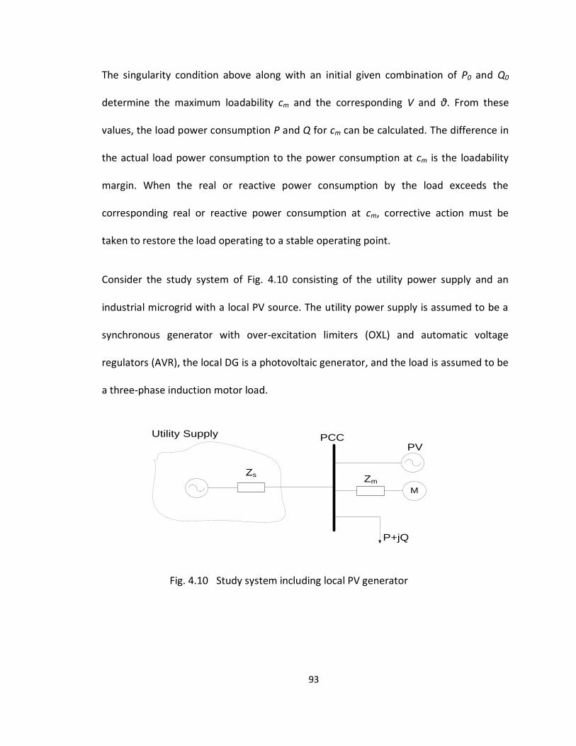
93
The singularity condition above along with an initial given combination of P0 and Q0
determine the maximum loadability cm and the corresponding V and θ. From these
values, the load power consumption P and Q for cm can be calculated. The difference in
the actual load power consumption to the power consumption at cm is the loadability
margin. When the real or reactive power consumption by the load exceeds the
corresponding real or reactive power consumption at cm, corrective action must be
taken to restore the load operating to a stable operating point.
Consider the study system of Fig. 4.10 consisting of the utility power supply and an
industrial microgrid with a local PV source. The utility power supply is assumed to be a
synchronous generator with over-excitation limiters (OXL) and automatic voltage
regulators (AVR), the local DG is a photovoltaic generator, and the load is assumed to be
a three-phase induction motor load.
Zs
M
Zm
P+jQ
PCCPV
Utility Supply
Fig. 4.10 Study system including local PV generator
94
The system can be represented by the sets of differential equations below:
(4.49)
(4.50)
(4.51)
(4.52)
where Fq and Ff are the transient reactance emf and field voltage emf of the generator
respectively. Toc is the open-circuit transient time constant, Ld is the winding self
inductance, L’d is the transient self winding inductance and id is the current produced by
the generator. G and T are characteristics of the OXL and AVR of the generator while V0
and Vg are the reference voltage of the AVR and the terminal voltage of the generator
respectively.
The loadability limit, Lm, determined by the SNB and Hopf bifurcation surface, is defined
in terms of the real and reactive power demands of the system. The bifurcation
conditions for an industrial microgrid are examined separately for the short-term and
long-term models since the dynamics of the power system evolve over different
timescales.
95
4.3.1 Short-Term Voltage Instability
The approximate short-term dynamic model is given by:
(4.53)
(4.54)
Here, y is the vector of state variables describing the microgrid load bus voltages and
angles. As shown earlier, a necessary condition for the loadability limit of the microgrid,
assuming the state variables are fixed, is the singularity of gy. For a microgrid consisting
primarily of induction motors fitting the exponential load model (a = b > 1), as is usually
the case industrial microgrids, then there is a single solution for every value of the
cumulative load demand in eq. (4.43) and there is no loadability limit. In this case, one
can apply the implicit function theorem to eq. (4.53) [84] to get:
(4.55)
The equilibrium conditions of eq. (4.53) for a fixed p are
(4.56)
(4.57)
At the equilibrium, the unreduced Jacobian is
(4.58)
96
Recalling that the necessary condition for SNB is the singularity of the state Jacobian,
the singularity of the unreduced Jacobian is the condition that induces the SNB of the
short-term dynamics. This coincides with the necessary condition for the loadability
limit when the system is in steady-state.
The short-term model considers the dynamics of fast-acting devices only, and assumes
that the slowly varying parameters are in steady-state. Some power system components
whose dynamics involve in the short-term time scale include synchronous generators,
automatic voltage regulators (AVRs), induction motors, HVDC components and static
VAR compensators (SVCs).
Short-term voltage instability can result from voltage sags due to the starting or
reacceleration of motors. During startup, the motor impedance consists of the winding
resistance in series with the inductive reactance, but the resistance is usually neglected
since it is much smaller than the reactance. Before the motor is energized, the rotor is at
a standstill and there is no counter-emf. However, as the rotors start to accelerate, a
counter-emf builds, effectively reducing the voltage across the motor windings and thus
limiting the current as shown in Fig. 4.12. As a result, the starting current is much
smaller than the running current and can typically be up to 5 or 6 times larger in
magnitude [71].
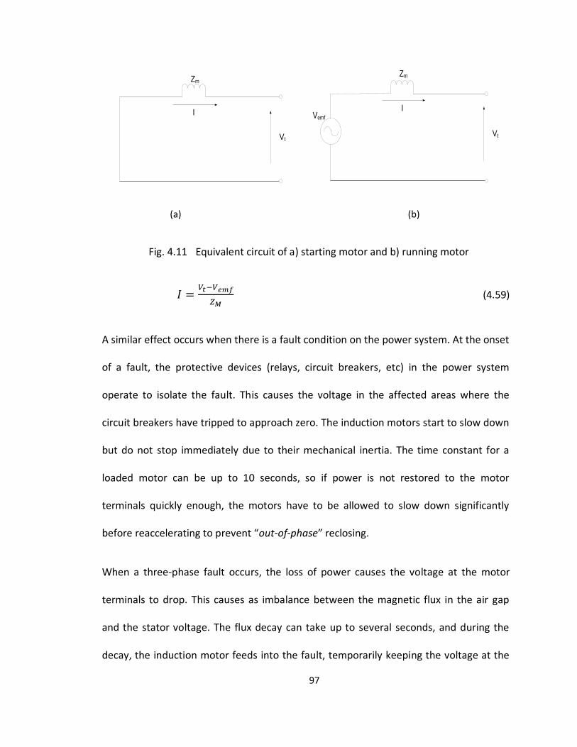
97
Zm
I
Vt
Zm
I
Vt
Vemf
(a) (b)
Fig. 4.11 Equivalent circuit of a) starting motor and b) running motor
(4.59)
A similar effect occurs when there is a fault condition on the power system. At the onset
of a fault, the protective devices (relays, circuit breakers, etc) in the power system
operate to isolate the fault. This causes the voltage in the affected areas where the
circuit breakers have tripped to approach zero. The induction motors start to slow down
but do not stop immediately due to their mechanical inertia. The time constant for a
loaded motor can be up to 10 seconds, so if power is not restored to the motor
terminals quickly enough, the motors have to be allowed to slow down significantly
before reaccelerating to prevent “out-of-phase” reclosing.
When a three-phase fault occurs, the loss of power causes the voltage at the motor
terminals to drop. This causes as imbalance between the magnetic flux in the air gap
and the stator voltage. The flux decay can take up to several seconds, and during the
decay, the induction motor feeds into the fault, temporarily keeping the voltage at the
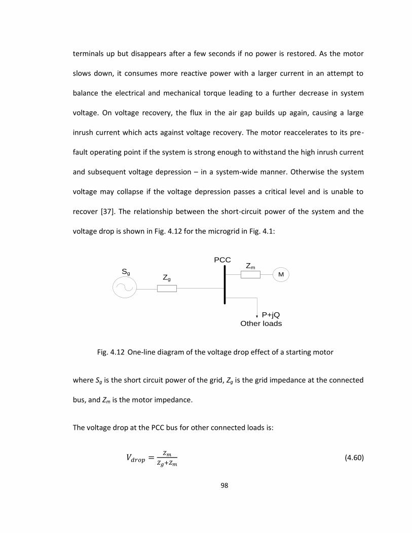
98
terminals up but disappears after a few seconds if no power is restored. As the motor
slows down, it consumes more reactive power with a larger current in an attempt to
balance the electrical and mechanical torque leading to a further decrease in system
voltage. On voltage recovery, the flux in the air gap builds up again, causing a large
inrush current which acts against voltage recovery. The motor reaccelerates to its pre-
fault operating point if the system is strong enough to withstand the high inrush current
and subsequent voltage depression – in a system-wide manner. Otherwise the system
voltage may collapse if the voltage depression passes a critical level and is unable to
recover [37]. The relationship between the short-circuit power of the system and the
voltage drop is shown in Fig. 4.12 for the microgrid in Fig. 4.1:
ZgM
Zm
P+jQ
PCC
Other loads
Sg
Fig. 4.12 One-line diagram of the voltage drop effect of a starting motor
where Sg is the short circuit power of the grid, Zg is the grid impedance at the connected
bus, and Zm is the motor impedance.
The voltage drop at the PCC bus for other connected loads is:
(4.60)
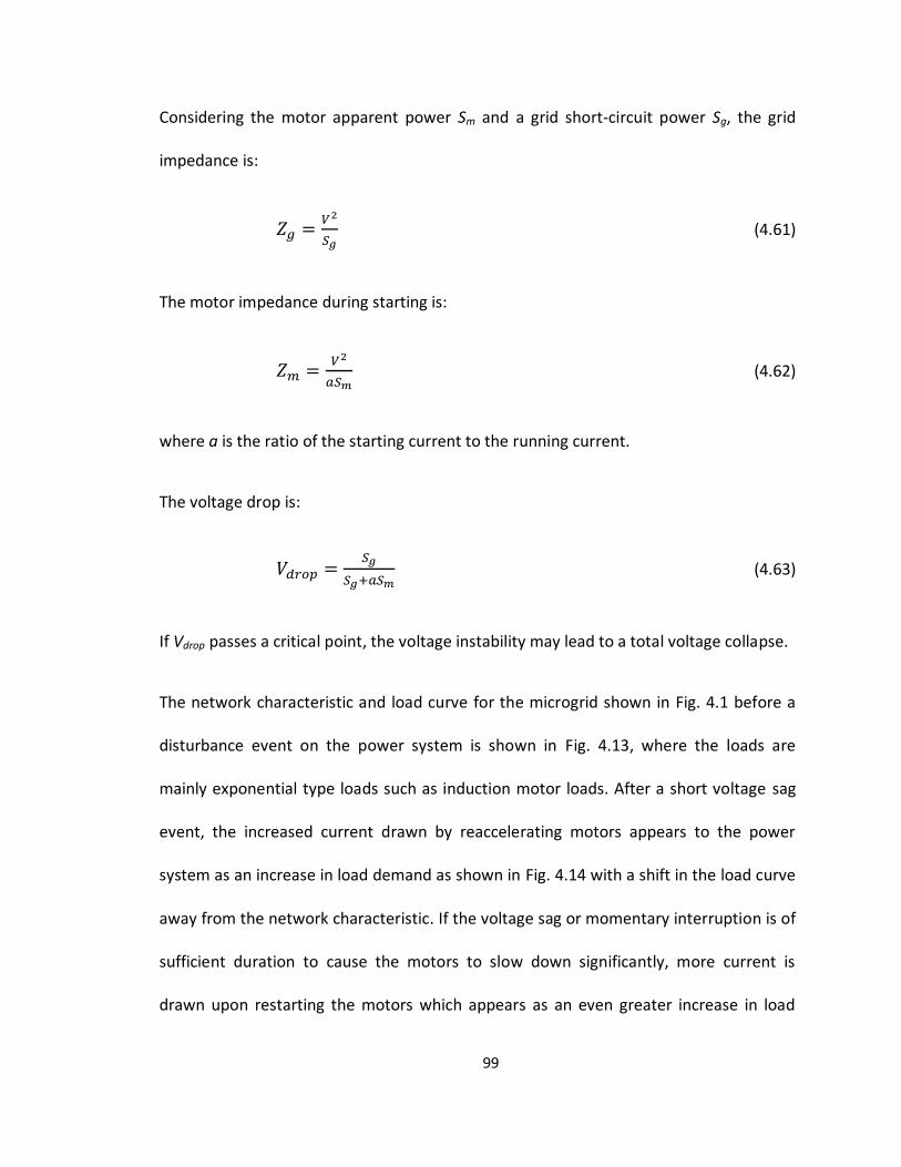
99
Considering the motor apparent power Sm and a grid short-circuit power Sg, the grid
impedance is:
(4.61)
The motor impedance during starting is:
(4.62)
where a is the ratio of the starting current to the running current.
The voltage drop is:
(4.63)
If Vdrop passes a critical point, the voltage instability may lead to a total voltage collapse.
The network characteristic and load curve for the microgrid shown in Fig. 4.1 before a
disturbance event on the power system is shown in Fig. 4.13, where the loads are
mainly exponential type loads such as induction motor loads. After a short voltage sag
event, the increased current drawn by reaccelerating motors appears to the power
system as an increase in load demand as shown in Fig. 4.14 with a shift in the load curve
away from the network characteristic. If the voltage sag or momentary interruption is of
sufficient duration to cause the motors to slow down significantly, more current is
drawn upon restarting the motors which appears as an even greater increase in load

100
demand until the load demand no longer intersects the network characteristic as shown
in Fig. 4.15. The microgrid experiences short-term voltage instability when the load
curve passes the network bifurcation surface. A local PV generator is used to extend the
network curve as shown in Fig. 4.16 so that the load curve now intersects the network
characteristic and voltage stability is restored.
The maximum size of the local PV generator is determined by the difference between
the initial P0 and Q0 and the P and Q values at the maximum loadability limit cm.
(4.64)
and
(4.65)
Any values of the local PV generator greater than max Ppv and Qpv will likely lead to
overvoltages at the PCC during light loading, resulting in the utility disconnection of the
PV generator and the subsequent reduction in the voltage stability margin.
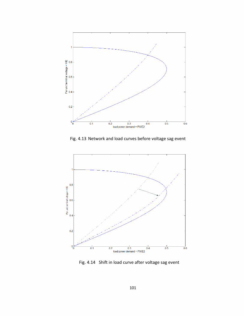
101
Fig. 4.13 Network and load curves before voltage sag event
Fig. 4.14 Shift in load curve after voltage sag event
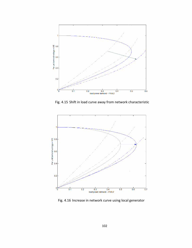
102
Fig. 4.15 Shift in load curve away from network characteristic
Fig. 4.16 Increase in network curve using local generator
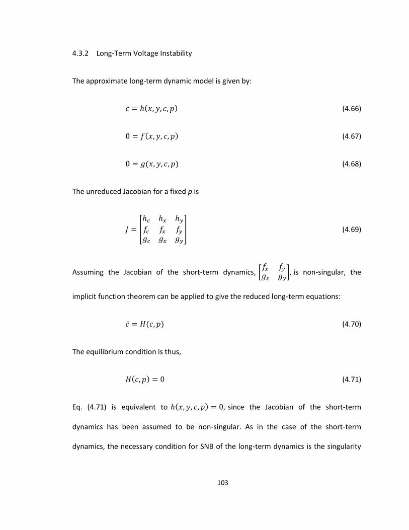
103
4.3.2 Long-Term Voltage Instability
The approximate long-term dynamic model is given by:
(4.66)
(4.67)
(4.68)
The unreduced Jacobian for a fixed p is
(4.69)
Assuming the Jacobian of the short-term dynamics,
is non-singular, the
implicit function theorem can be applied to give the reduced long-term equations:
(4.70)
The equilibrium condition is thus,
(4.71)
Eq. (4.71) is equivalent to since the Jacobian of the short-term
dynamics has been assumed to be non-singular. As in the case of the short-term
dynamics, the necessary condition for SNB of the long-term dynamics is the singularity
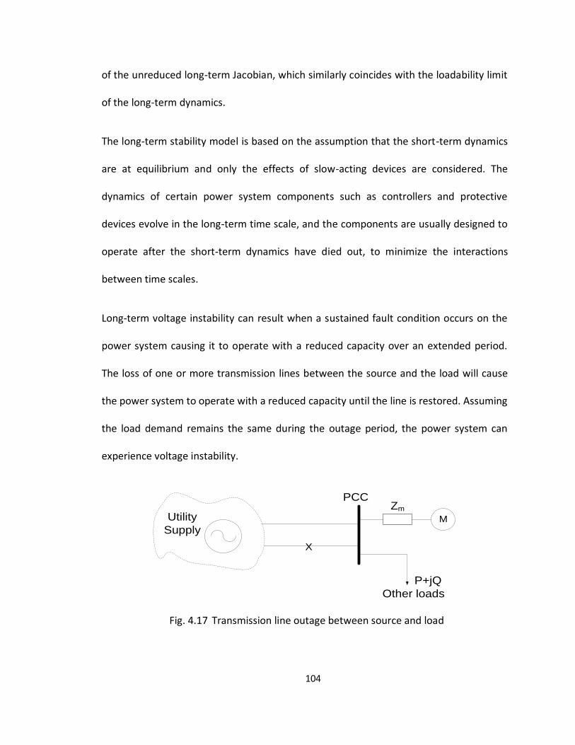
104
of the unreduced long-term Jacobian, which similarly coincides with the loadability limit
of the long-term dynamics.
The long-term stability model is based on the assumption that the short-term dynamics
are at equilibrium and only the effects of slow-acting devices are considered. The
dynamics of certain power system components such as controllers and protective
devices evolve in the long-term time scale, and the components are usually designed to
operate after the short-term dynamics have died out, to minimize the interactions
between time scales.
Long-term voltage instability can result when a sustained fault condition occurs on the
power system causing it to operate with a reduced capacity over an extended period.
The loss of one or more transmission lines between the source and the load will cause
the power system to operate with a reduced capacity until the line is restored. Assuming
the load demand remains the same during the outage period, the power system can
experience voltage instability.
M
Zm
P+jQ
PCC
Other loads
Utility
Supply
X
Fig. 4.17 Transmission line outage between source and load
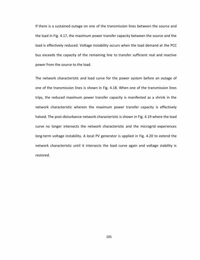
105
If there is a sustained outage on one of the transmission lines between the source and
the load in Fig. 4.17, the maximum power transfer capacity between the source and the
load is effectively reduced. Voltage instability occurs when the load demand at the PCC
bus exceeds the capacity of the remaining line to transfer sufficient real and reactive
power from the source to the load.
The network characteristic and load curve for the power system before an outage of
one of the transmission lines is shown in Fig. 4.18. When one of the transmission lines
trips, the reduced maximum power transfer capacity is manifested as a shrink in the
network characteristic wherein the maximum power transfer capacity is effectively
halved. The post-disturbance network characteristic is shown in Fig. 4.19 where the load
curve no longer intersects the network characteristic and the microgrid experiences
long-term voltage instability. A local PV generator is applied in Fig. 4.20 to extend the
network characteristic until it intersects the load curve again and voltage stability is
restored.
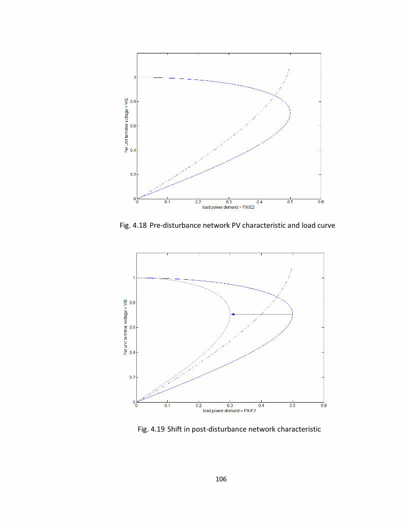
106
Fig. 4.18 Pre-disturbance network PV characteristic and load curve
Fig. 4.19 Shift in post-disturbance network characteristic
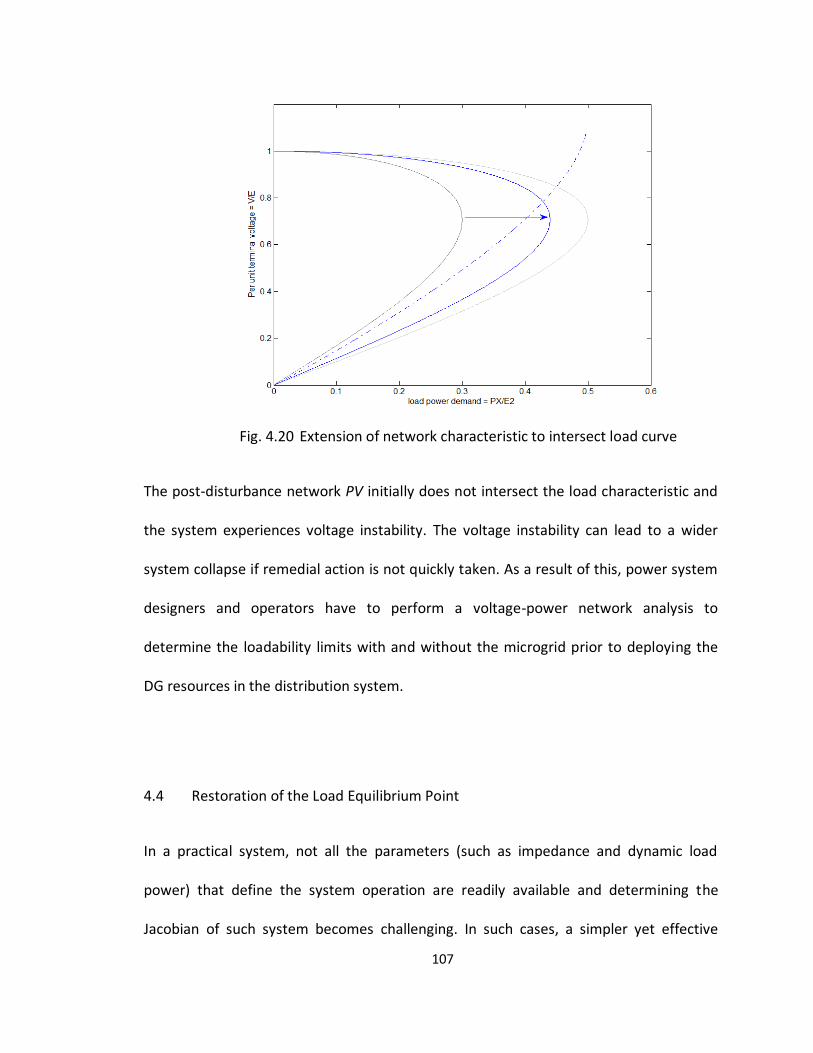
107
Fig. 4.20 Extension of network characteristic to intersect load curve
The post-disturbance network PV initially does not intersect the load characteristic and
the system experiences voltage instability. The voltage instability can lead to a wider
system collapse if remedial action is not quickly taken. As a result of this, power system
designers and operators have to perform a voltage-power network analysis to
determine the loadability limits with and without the microgrid prior to deploying the
DG resources in the distribution system.
4.4 Restoration of the Load Equilibrium Point
In a practical system, not all the parameters (such as impedance and dynamic load
power) that define the system operation are readily available and determining the
Jacobian of such system becomes challenging. In such cases, a simpler yet effective
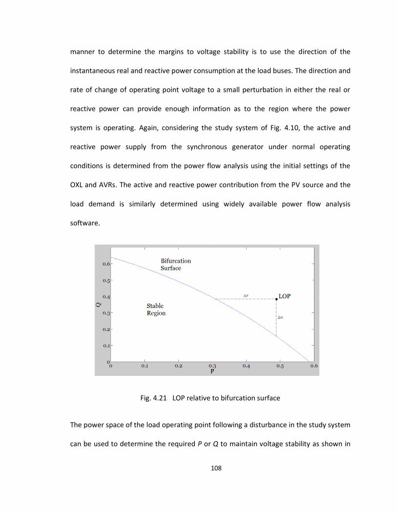
108
manner to determine the margins to voltage stability is to use the direction of the
instantaneous real and reactive power consumption at the load buses. The direction and
rate of change of operating point voltage to a small perturbation in either the real or
reactive power can provide enough information as to the region where the power
system is operating. Again, considering the study system of Fig. 4.10, the active and
reactive power supply from the synchronous generator under normal operating
conditions is determined from the power flow analysis using the initial settings of the
OXL and AVRs. The active and reactive power contribution from the PV source and the
load demand is similarly determined using widely available power flow analysis
software.
Fig. 4.21 LOP relative to bifurcation surface
The power space of the load operating point following a disturbance in the study system
can be used to determine the required P or Q to maintain voltage stability as shown in

109
Fig 4.21. If the load operating point (LOP) falls outside the feasible region following the
disturbance then corrective action is required to return the operating point to the
feasible region on the left side of the bifurcation surface. The feasible operating point
can be restored either by increasing the active power, ∆P, or increasing the reactive
compensation, ∆Q, at the bus, although since increasing the active power will tend to
raise the voltage at the PCC beyond acceptable limits, the latter option is preferable.
The Euclidean distance, ∆Q, to the bifurcation surface is then calculated to determine
the amount of reactive compensation required to restore the load equilibrium point.
110
5. VOLTAGE STABILITY ENHANCEMENT USING REACTIVE POWER CONTROL
This chapter investigates the dynamic voltage impact when converter-interfaced DGs
are connected to the power system. Converter-interfaced DGs are typically operated at
unity power factor and are disconnected from the rest of the power system upon a fault
occurrence. The basic DG controller is used to study the voltage response at the PCC to
fault occurrences in DG-embedded power systems. A novel real-time dynamic reactive
power controller (DPRC) that controls the converter-interfaced DG to output real or
reactive power depending on the short-term and long-tem voltage stability margins is
proposed. The maximum and minimum real and reactive power support permissible
from the DG is determined from the bifurcation analysis and is used as the limiting
factors in controlling the real and reactive power contribution from the PV source. The
first stage of the controller regulates the voltage output based on instantaneous power
theory to prevent overvoltage at the point-of-common coupling (PCC) while the second
stage regulates the reactive power supply by means of power factor and reactive
current droop control. The DRPC is implemented in PSCAD and the voltage response is
compared to the operation of the basic controller. The advantage of dynamic control is
demonstrated as the controller is able to respond to voltage variations in real-time and
maintain the output of the grid-tied DG within acceptable limits.

111
5.1 Microgrid Controller Modeling
This section focuses on operation of the DRPC to maintain the power system voltage
stability. The DRPC is implemented in the industrial microgrid shown in Fig. 5.1. The
industrial microgrid consists of:
The PV source is connected to the PCC via the DRPC and an inverter. The
PV source has an MPPT and is initially set to generate real power only.
The total load is represented with one aggregate load with real and
reactive power demand. They are modeled as constant impedance and
constant power loads.
The reactive power is initially supplied by the grid via the PCC. The DRPC
is later used to control the PV source to supply both real and reactive
power to balance the reactive power shortfall from the grid.
The power imbalance scenarios are simulated first by changing the active
and reactive power demand of the load to indicate a gradual increase in
load, then by applying a three-phase fault on the grid side to indicate a
short duration system disturbance.
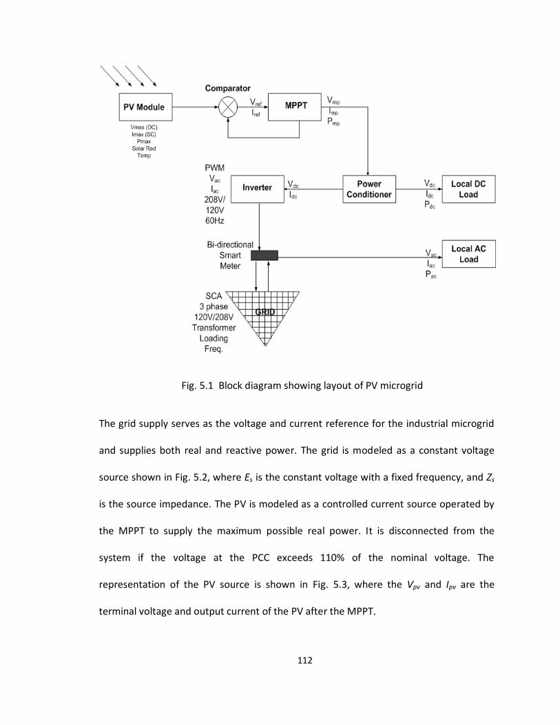
112
Fig. 5.1 Block diagram showing layout of PV microgrid
The grid supply serves as the voltage and current reference for the industrial microgrid
and supplies both real and reactive power. The grid is modeled as a constant voltage
source shown in Fig. 5.2, where Es is the constant voltage with a fixed frequency, and Zs
is the source impedance. The PV is modeled as a controlled current source operated by
the MPPT to supply the maximum possible real power. It is disconnected from the
system if the voltage at the PCC exceeds 110% of the nominal voltage. The
representation of the PV source is shown in Fig. 5.3, where the Vpv and Ipv are the
terminal voltage and output current of the PV after the MPPT.
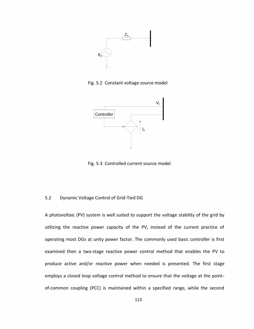
113
Zs
Es
Fig. 5.2 Constant voltage source model
Controller
Vt
Is
Fig. 5.3 Controlled current source model
5.2 Dynamic Voltage Control of Grid-Tied DG
A photovoltaic (PV) system is well suited to support the voltage stability of the grid by
utilizing the reactive power capacity of the PV, instead of the current practice of
operating most DGs at unity power factor. The commonly used basic controller is first
examined then a two-stage reactive power control method that enables the PV to
produce active and/or reactive power when needed is presented. The first stage
employs a closed loop voltage control method to ensure that the voltage at the point-
of-common coupling (PCC) is maintained within a specified range, while the second

114
stage controls the active and reactive power output of the PV inverter by adjusting the
transformed real and reactive currents of the instantaneous power at the PCC based on
the power factor measurement of the instantaneous voltage and reference current. The
reactive power control method is implemented in PSCAD and the voltage stability
enhancement of the PV system is demonstrated.
5.2.1 Voltage Control using Basic Controller
The role of the central generators is to maintain the power balance in the entire system
and supply any deficient real and reactive power demand of the microgrid. The grid
supply represented by the constant voltage source (Fig. 5.2) must supply the required
active and reactive power requirements of the microgrid within the maximum power
transfer limits of the power system, which is inversely proportional to the source
impedance Zs (Section 4.1). The PV source represented by the controlled current source
(Fig. 5.3) supplies active power to the microgrid within the acceptable voltage limits at
the PCC. The basic functionality of the controller is shown in Fig. 5.4.
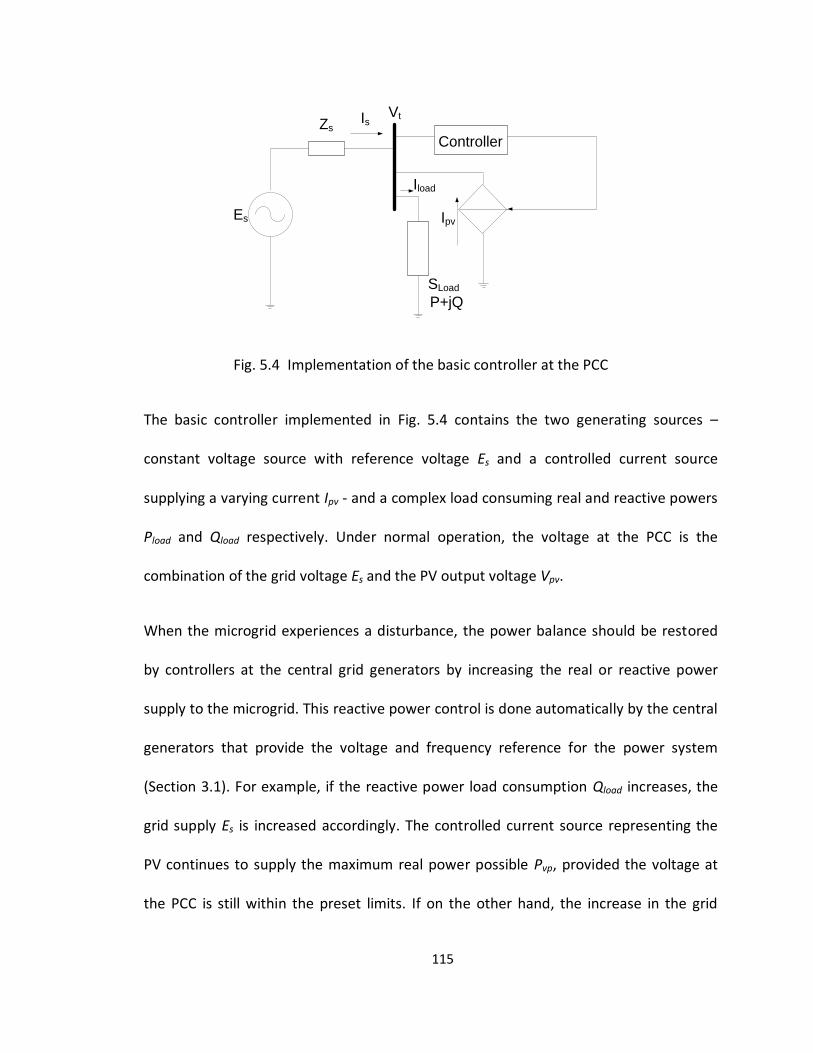
115
Controller
Vt
Ipv
SLoad
P+jQ
Zs
Es
Is
Iload
Fig. 5.4 Implementation of the basic controller at the PCC
The basic controller implemented in Fig. 5.4 contains the two generating sources –
constant voltage source with reference voltage Es and a controlled current source
supplying a varying current Ipv - and a complex load consuming real and reactive powers
Pload and Qload respectively. Under normal operation, the voltage at the PCC is the
combination of the grid voltage Es and the PV output voltage Vpv.
When the microgrid experiences a disturbance, the power balance should be restored
by controllers at the central grid generators by increasing the real or reactive power
supply to the microgrid. This reactive power control is done automatically by the central
generators that provide the voltage and frequency reference for the power system
(Section 3.1). For example, if the reactive power load consumption Qload increases, the
grid supply Es is increased accordingly. The controlled current source representing the
PV continues to supply the maximum real power possible Pvp, provided the voltage at
the PCC is still within the preset limits. If on the other hand, the increase in the grid
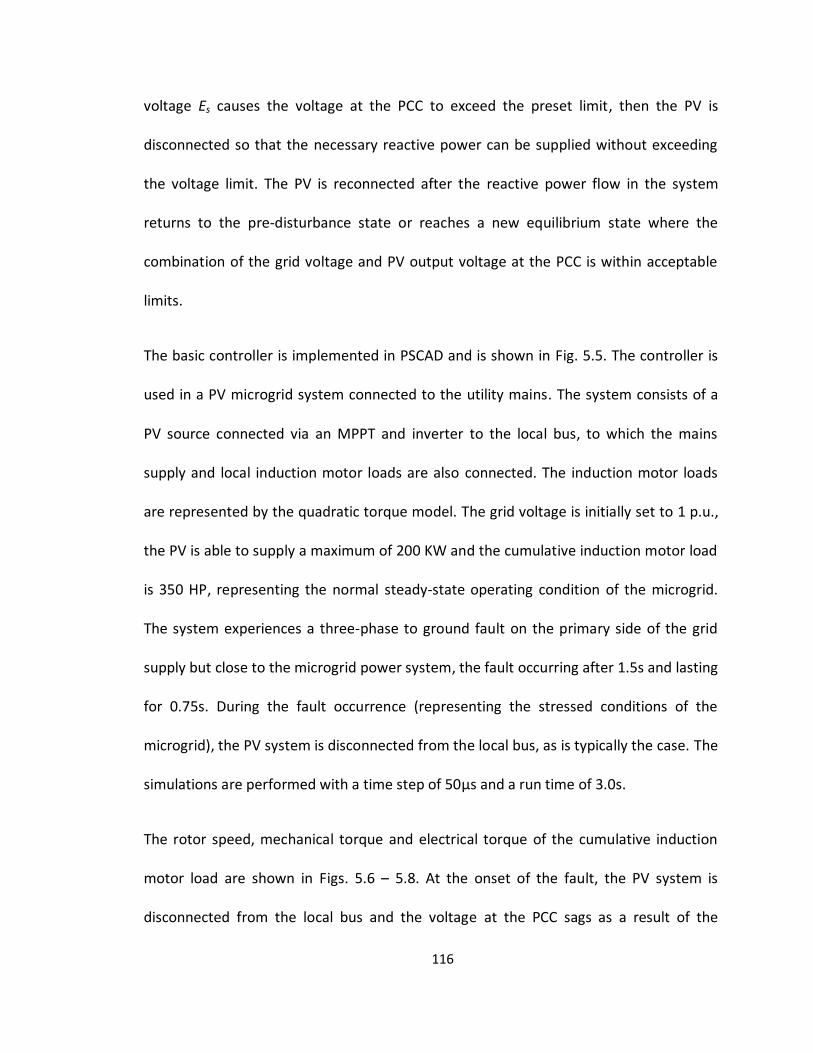
116
voltage Es causes the voltage at the PCC to exceed the preset limit, then the PV is
disconnected so that the necessary reactive power can be supplied without exceeding
the voltage limit. The PV is reconnected after the reactive power flow in the system
returns to the pre-disturbance state or reaches a new equilibrium state where the
combination of the grid voltage and PV output voltage at the PCC is within acceptable
limits.
The basic controller is implemented in PSCAD and is shown in Fig. 5.5. The controller is
used in a PV microgrid system connected to the utility mains. The system consists of a
PV source connected via an MPPT and inverter to the local bus, to which the mains
supply and local induction motor loads are also connected. The induction motor loads
are represented by the quadratic torque model. The grid voltage is initially set to 1 p.u.,
the PV is able to supply a maximum of 200 KW and the cumulative induction motor load
is 350 HP, representing the normal steady-state operating condition of the microgrid.
The system experiences a three-phase to ground fault on the primary side of the grid
supply but close to the microgrid power system, the fault occurring after 1.5s and lasting
for 0.75s. During the fault occurrence (representing the stressed conditions of the
microgrid), the PV system is disconnected from the local bus, as is typically the case. The
simulations are performed with a time step of 50μs and a run time of 3.0s.
The rotor speed, mechanical torque and electrical torque of the cumulative induction
motor load are shown in Figs. 5.6 – 5.8. At the onset of the fault, the PV system is
disconnected from the local bus and the voltage at the PCC sags as a result of the
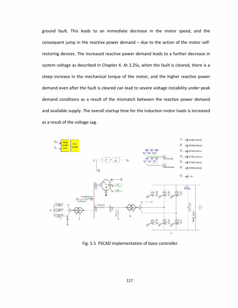
117
ground fault. This leads to an immediate decrease in the motor speed, and the
consequent jump in the reactive power demand – due to the action of the motor self-
restoring devices. The increased reactive power demand leads to a further decrease in
system voltage as described in Chapter 4. At 2.25s, when the fault is cleared, there is a
steep increase in the mechanical torque of the motor, and the higher reactive power
demand even after the fault is cleared can lead to severe voltage instability under peak
demand conditions as a result of the mismatch between the reactive power demand
and available supply. The overall startup time for the induction motor loads is increased
as a result of the voltage sag.
Fig. 5.5 PSCAD implementation of basic controller
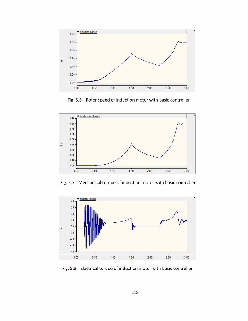
118
Fig. 5.6 Rotor speed of induction motor with basic controller
Fig. 5.7 Mechanical torque of induction motor with basic controller
Fig. 5.8 Electrical torque of induction motor with basic controller
119
5.2.2 Real-Time Dynamic Reactive Power Controller
A novel dynamic reactive power controller (DPRC) that operates the PV source in a
manner that ensures the PV remains online through system disturbances is proposed in
place of the basic controller that disconnects the PV source during a fault occurrence or
when the voltage rises at the PCC rises above acceptable levels. The DRPC operates the
PV inverter using a two-stage voltage vs. reactive current droop control method. The
first stage implements the voltage control by means of a closed-loop control method
where the measured grid voltage (Vg) at the PCC is compared with a preset upper and
lower limit range set by the operator, and if Vg is found out of range and with a lagging
power factor, the reactive power output of the inverter is increased. Alternatively, if Vg
is out of range but with a leading power factor, the real power output of the inverter is
lowered. The reference real and reactive currents are determined as follows:
The instantaneous voltage and current at the inverter-grid interface is measured as [89]
(5.1)
(5.2)
and the instantaneous power,
(5.3)
(5.4)
120
(5.5)
The current in terms of and is
(5.6)
From eq. (5.6), the real and reactive components of the current using coordinate
transform are respectively
(5.7)
(5.8)
where id is in phase with Va(t) and iq is perpendicular to Va(t) and I = id + iq. If the
coordinate transform is applied to the voltage:
(5.9)
The instantaneous power is expressed as
(5.10)
The three-phase instantaneous power is obtained as
121
where Po is the instantaneous zero-sequence power.
(5.11)
(5.12)
The instantaneous real and reactive power represented in matrix form is
(5.13)
and the reference current
(5.14)
The control algorithm for the DRPC using the derived real and reactive reference current
is shown in Fig. 5.9. The limits for the real and reactive power output are set based on
the max and min ∆P and ∆Q calculated from the bifurcation stability analysis in Chapter
4. If the voltage at the PCC is capacitive and the load operating point is close to the
stability margin, then option 1 of reducing the PV DC voltage via direct MPPT control is
preferred.
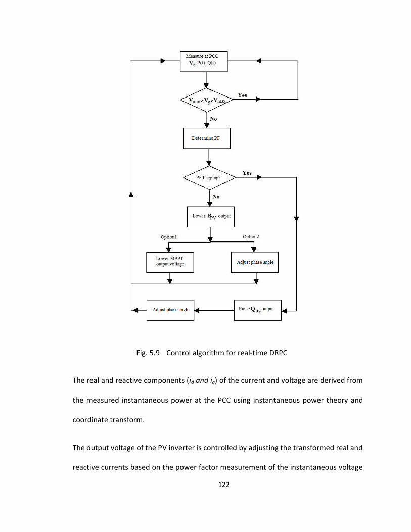
122
Fig. 5.9 Control algorithm for real-time DRPC
The real and reactive components (id and iq) of the current and voltage are derived from
the measured instantaneous power at the PCC using instantaneous power theory and
coordinate transform.
The output voltage of the PV inverter is controlled by adjusting the transformed real and
reactive currents based on the power factor measurement of the instantaneous voltage

123
and reference current. In the case of undervoltage at the PCC, the transformed reactive
current, iq, is increased while the transformed real current, id, is kept the same to output
more inductive reactive power from the PV. In the case of overvoltage, id is decreased
while iq is kept the same to reduce the output voltage from the PV. The adjusted id
and/or iq are transformed back to the abc reference frame and used for the inverter
PWM control.
The inverter output voltage is synchronized to the grid voltage and frequency using a PI
controller. The measured id and iq currents are compared to the set reference id and iq
currents, and the current control error is fed into the PI controller and comparator,
where the PWM modulation gain kp is generated. The utility frequency, ωu = 2πfu,
sensed by a phase-lock loop (PLL) circuit, is combined with the PWM modulation gain
and angle to generate the inverter output voltage, kpVinvsin(ωut + α). The desired
magnitude of the inverter voltage is realized by adjusting the set reference id and iq
currents based on the droop, θ, of the voltage vs. reactive power at the PCC shown as in
Fig. 5.10. The overall control scheme and PI controller are shown in Figs. 5.11 and 5.12.
Fig. 5.10 Voltage set point vs. reactive power droop
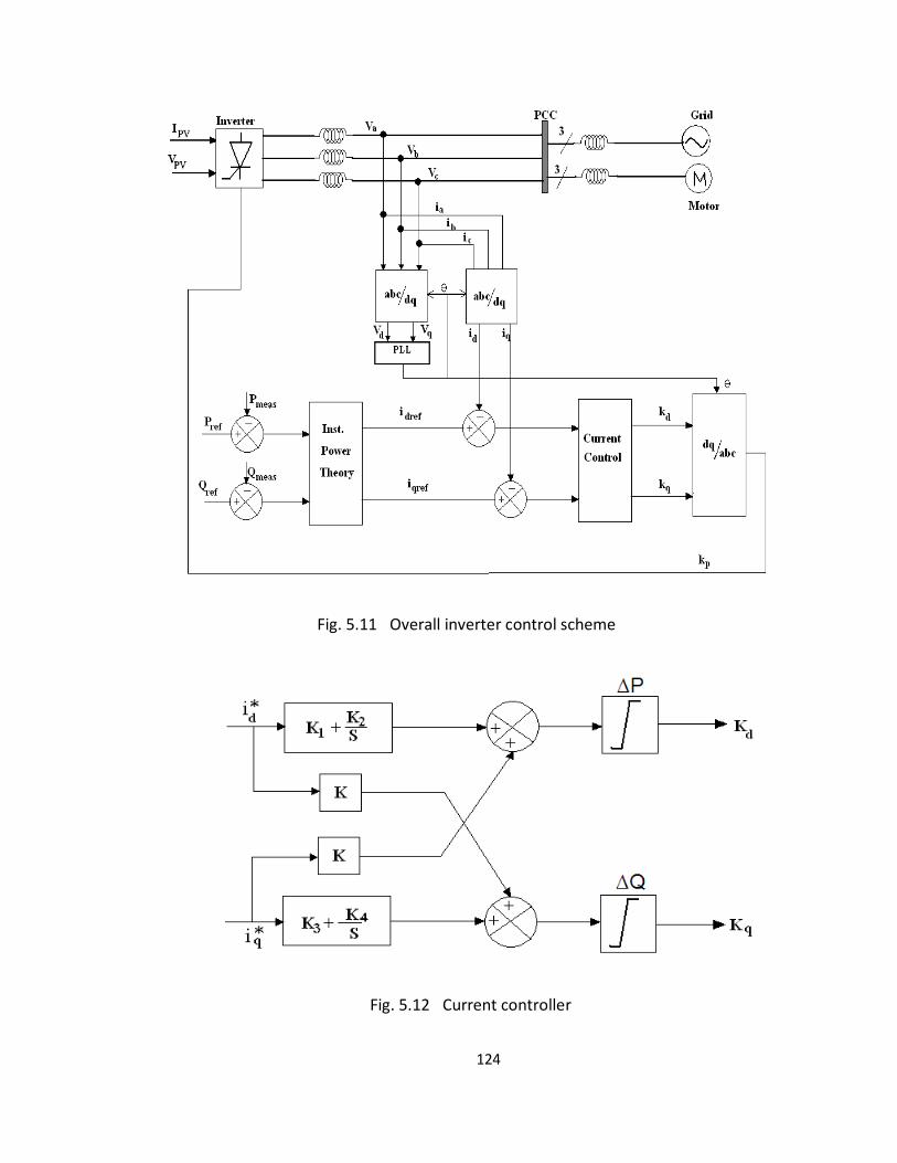
124
Fig. 5.11 Overall inverter control scheme
Fig. 5.12 Current controller
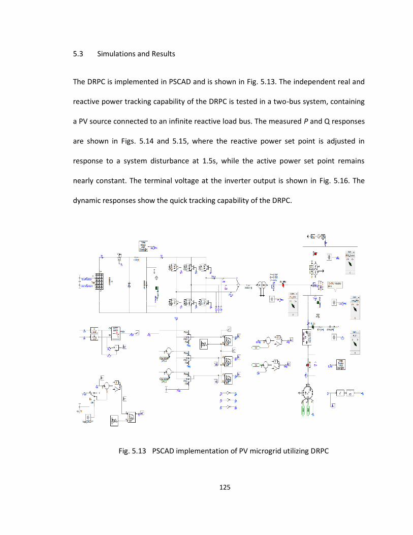
125
5.3 Simulations and Results
The DRPC is implemented in PSCAD and is shown in Fig. 5.13. The independent real and
reactive power tracking capability of the DRPC is tested in a two-bus system, containing
a PV source connected to an infinite reactive load bus. The measured P and Q responses
are shown in Figs. 5.14 and 5.15, where the reactive power set point is adjusted in
response to a system disturbance at 1.5s, while the active power set point remains
nearly constant. The terminal voltage at the inverter output is shown in Fig. 5.16. The
dynamic responses show the quick tracking capability of the DRPC.
Fig. 5.13 PSCAD implementation of PV microgrid utilizing DRPC
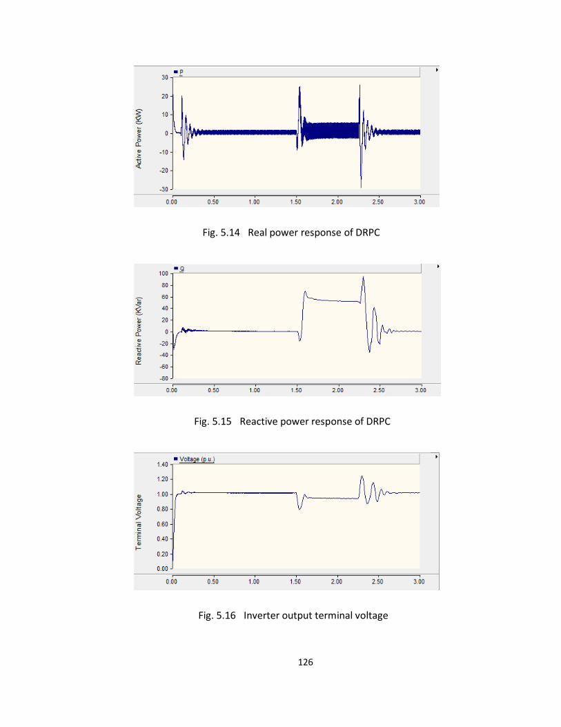
126
Fig. 5.14 Real power response of DRPC
Fig. 5.15 Reactive power response of DRPC
Fig. 5.16 Inverter output terminal voltage

127
The DRPC is implemented in the same system as was done for the basic controller. The
grid voltage is initially set to 1 p.u., while the PV is now able to supply up to +100 KVar
and a maximum of 150 KW. The cumulative induction motor load remains the same at
350 HP, representing the normal steady-state operating condition of the microgrid. The
system experiences a disturbance at 1.5s in the form of a three-phase to ground fault
that causes momentary voltage sag lasting for 0.75s. During the fault occurrence
(representing the stressed conditions of the microgrid), the PV system remains
connected to the local load bus via the DRPC. The simulations are performed with a time
step of 50μs and a run time of 3.0s.
The rotor speed, mechanical torque and electrical torque of the cumulative induction
motor load are shown in Figs. 5.17 – 5.19. At the onset of the fault, the DRPC is able to
supply the increased reactive power demand of the motor before the rotor speed
decrease significantly as shown in Fig. 5.17. The mechanical and electrical torques of the
motor are maintained during the fault as shown in Figs. 5.18 and 5.19 respectively,
allowing the motor to fully start. The system voltage is therefore less stressed during
and immediately after the fault is cleared. This approach eliminates the need for load
shedding or staggered motor start during peak demand conditions on the grid.
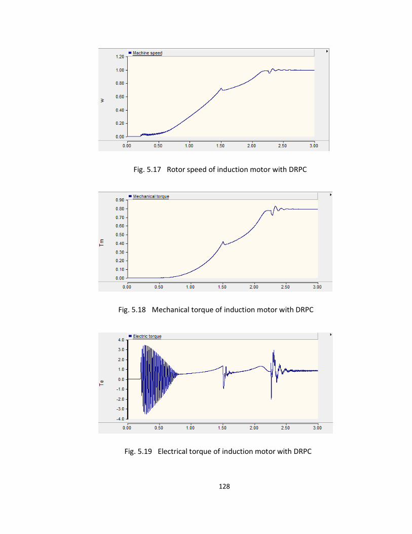
128
Fig. 5.17 Rotor speed of induction motor with DRPC
Fig. 5.18 Mechanical torque of induction motor with DRPC
Fig. 5.19 Electrical torque of induction motor with DRPC
129
6. CASE STUDY FOR TAMPA LOWRY PARK ZOO MICROGRID
The effect of dynamic reactive power compensation is first investigated in an IEEE 13-
bus test feeder system and then for an industrial microgrid using data from an actual PV
installation in Tampa, FL. The PV microgrid is operated primarily as a peak load shaving
DG source but can be modified to incorporate the DRPC to support the local area
voltage stability. The system is simulated in EDSA to determine the power flow and thus
the steady-state voltage stability of the industrial microgrid and nearby buses with and
without the DRPC in operation. The scenarios investigated include the case where there
is no DG present in the power system, the case where DG is present but is used to
supply real power only to the load bus, and finally, the case where DG is present and is
used to supply both real and reactive power to the load bus. The chapter concludes by
analyzing the impact of the application of the DRPC control method on the steady-state
(long-term) load voltage stability in the presence of voltage sags and momentary
interruptions.
130
6.1 Description of the Study Systems
The widely-used IEEE 13-bus test feeder system is implemented in EDSA to determine
the power flows when active loads consisting of mainly induction motors are added to
the power system. The IEEE 13-bus test system is used in order to allow for easy
comparisons of the test results with other voltage control mechanisms and various load
configurations. A section of the Tampa Electric (TECO) distribution network is then
approximated to a 13-bus power system and is used to illustrate the voltage stability
enhancement application of DGs operated to independently regulate the real and
reactive power outputs using data from a real-life system. The power flow analyses in
this chapter are performed as the steady-state complement to the dynamic analysis
performed in Chapter 5.
6.2 IEEE 13-Bus Test Feeder System
The IEEE 13-bus test feeder system is a commonly used test system in power system
planning and analysis. The benefit of using this test system is to validate the power flow
simulations using tests results that are widely available in literature making the research
useful for comparison purposes. Although the 13-bus system is relatively small, the
voltage impact on a reasonably-sized distribution area can still be adequately captured.
The one-line diagram of the IEEE 13-bus system containing three DG sources is shown in
Fig. 6.1 and the load demand at each bus is presented in Table 6.1.
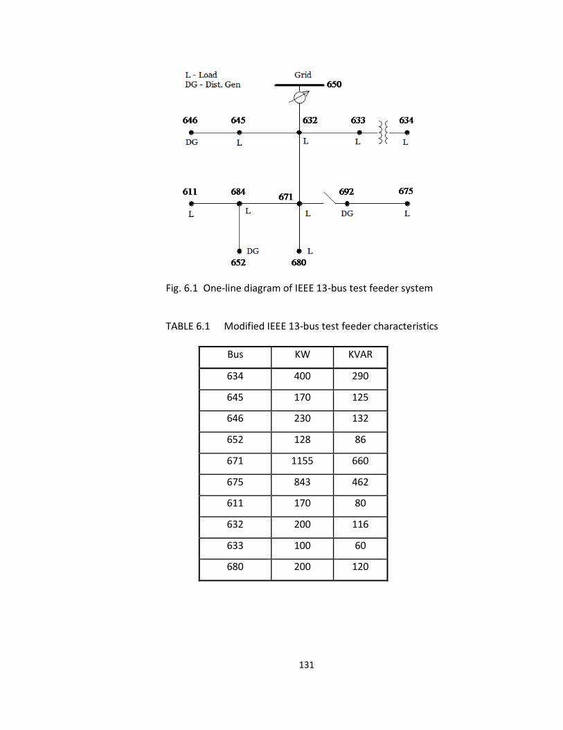
131
Fig. 6.1 One-line diagram of IEEE 13-bus test feeder system
TABLE 6.1 Modified IEEE 13-bus test feeder characteristics
Bus KW KVAR
634 400 290
645 170 125
646 230 132
652 128 86
671 1155 660
675 843 462
611 170 80
632 200 116
633 100 60
680 200 120
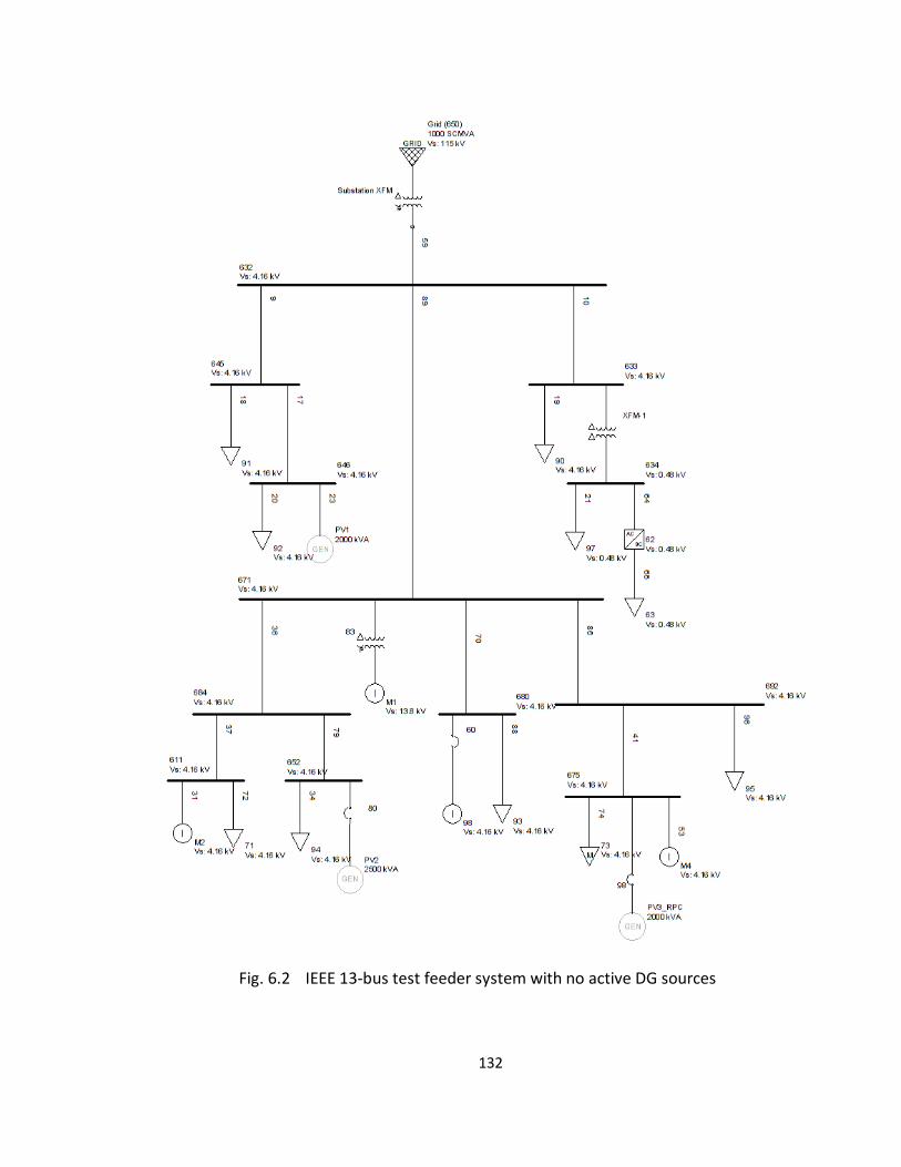
132
Fig. 6.2 IEEE 13-bus test feeder system with no active DG sources

133
The basic parameters are taken from [90] with slight modifications made at some buses.
The scenario of most interest is the case of peak load demand when there is little
reserve capacity left on the system. As such, there are no swing buses and every
generator is set with a reactive power limit. The generators are modeled in EDSA library
using the Park (dq) transformation parameters of the synchronous generator.
6.2.1 Voltage Impact without DG Sources
The IEEE 13-bus test feeder system implemented in EDSA is shown in Fig. 6.2. Initially,
the 13-bus system contains no DG sources (DG sources initially switched off in EDSA)
with only the main grid supplying the power, and all the other buses represented as
load buses. The motor loads at buses 611, 671, 675, and 680 indicate large industrial
induction motors (M1 – M4) and all other loads indicate fixed loads. All the induction
motors are assumed to be initially off while all the fixed loads are on. The induction
motor loads are all started at the same time indicating a post-fault scenario where all
the induction motors have previously come to a stop or slowed down significantly. The
pre-start, during starting, and post-start voltages for some buses are presented in Table
6.2 and Fig. 6.3. It is seen that the voltages at all the buses shown have unacceptably
low voltages during the starting process, mainly as a result of insufficient reactive power
supply from the grid.
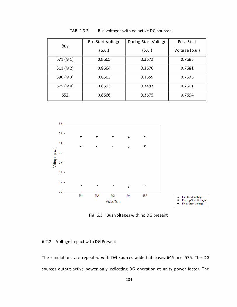
134
TABLE 6.2 Bus voltages with no active DG sources
Bus Pre-Start Voltage
(p.u.)
During-Start Voltage
(p.u.)
Post-Start
Voltage (p.u.)
671 (M1) 0.8665 0.3672 0.7683
611 (M2) 0.8664 0.3670 0.7681
680 (M3) 0.8663 0.3659 0.7675
675 (M4) 0.8593 0.3497 0.7601
652 0.8666 0.3675 0.7694
Fig. 6.3 Bus voltages with no DG present
6.2.2 Voltage Impact with DG Present
The simulations are repeated with DG sources added at buses 646 and 675. The DG
sources output active power only indicating DG operation at unity power factor. The
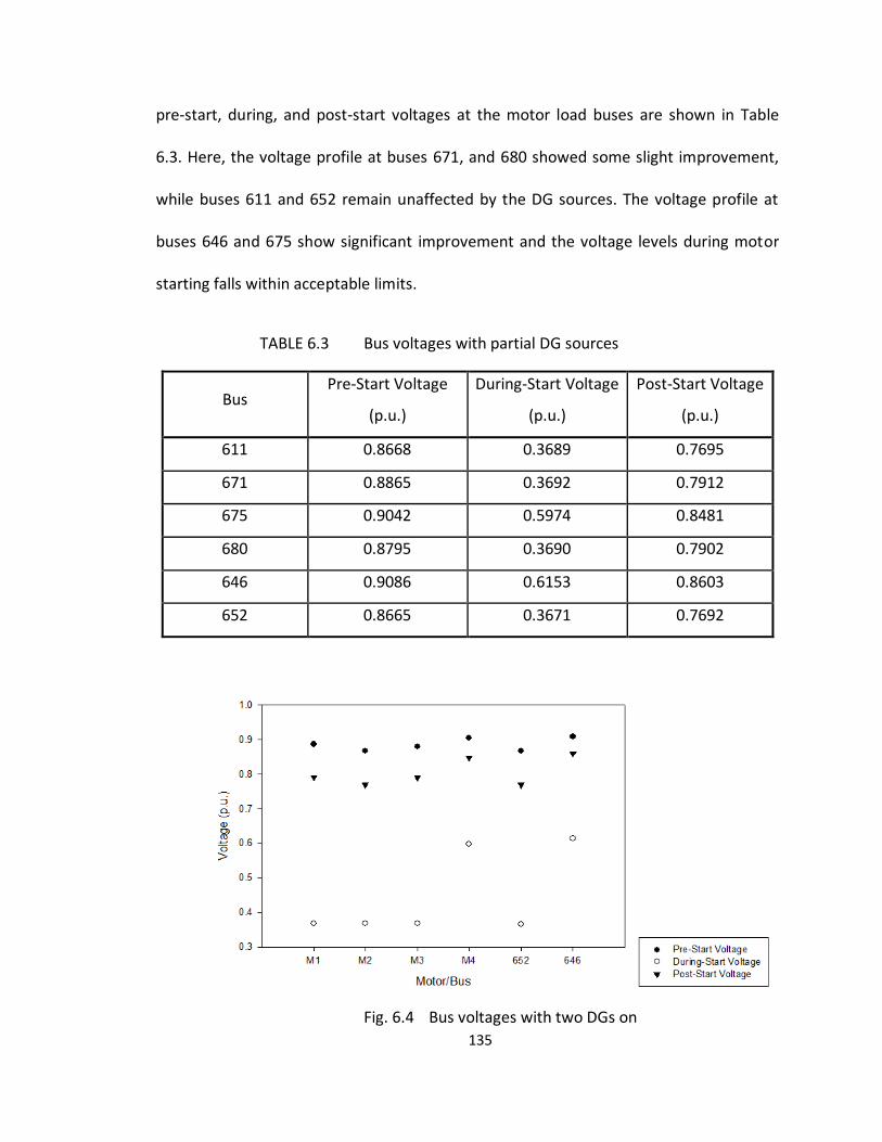
135
pre-start, during, and post-start voltages at the motor load buses are shown in Table
6.3. Here, the voltage profile at buses 671, and 680 showed some slight improvement,
while buses 611 and 652 remain unaffected by the DG sources. The voltage profile at
buses 646 and 675 show significant improvement and the voltage levels during motor
starting falls within acceptable limits.
TABLE 6.3 Bus voltages with partial DG sources
Bus Pre-Start Voltage
(p.u.)
During-Start Voltage
(p.u.)
Post-Start Voltage
(p.u.)
611 0.8668 0.3689 0.7695
671 0.8865 0.3692 0.7912
675 0.9042 0.5974 0.8481
680 0.8795 0.3690 0.7902
646 0.9086 0.6153 0.8603
652 0.8665 0.3671 0.7692
Fig. 6.4 Bus voltages with two DGs on
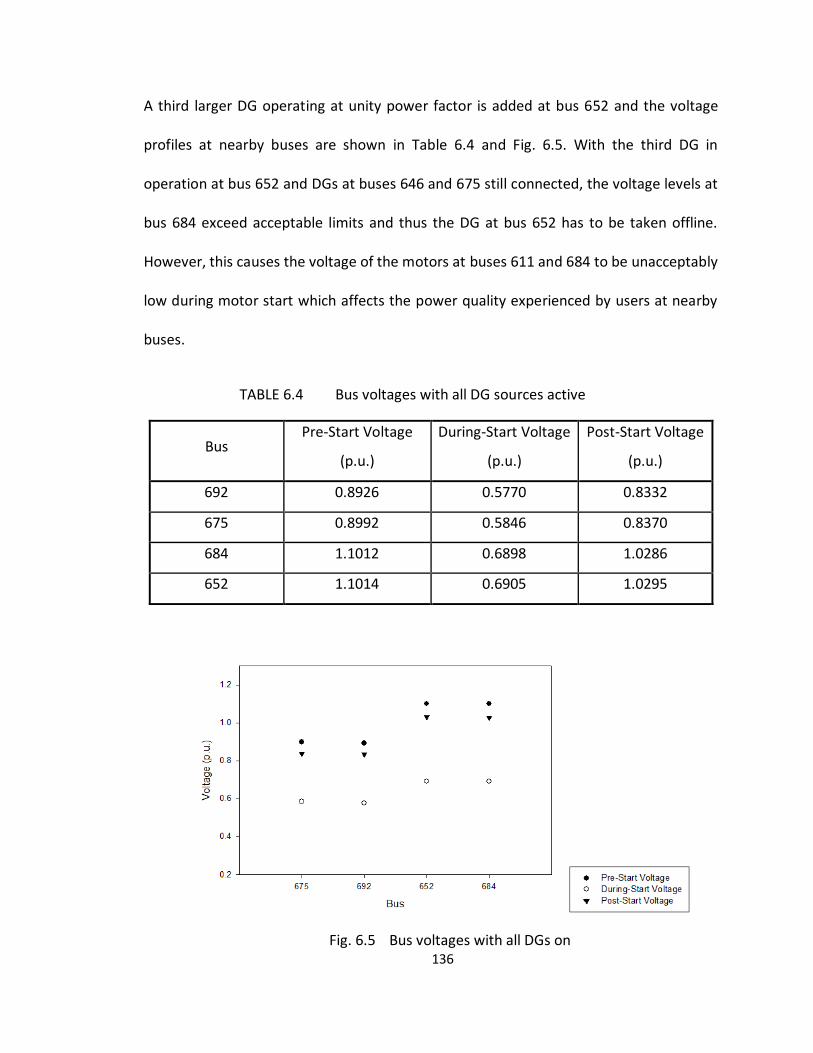
136
A third larger DG operating at unity power factor is added at bus 652 and the voltage
profiles at nearby buses are shown in Table 6.4 and Fig. 6.5. With the third DG in
operation at bus 652 and DGs at buses 646 and 675 still connected, the voltage levels at
bus 684 exceed acceptable limits and thus the DG at bus 652 has to be taken offline.
However, this causes the voltage of the motors at buses 611 and 684 to be unacceptably
low during motor start which affects the power quality experienced by users at nearby
buses.
TABLE 6.4 Bus voltages with all DG sources active
Bus Pre-Start Voltage
(p.u.)
During-Start Voltage
(p.u.)
Post-Start Voltage
(p.u.)
692 0.8926 0.5770 0.8332
675 0.8992 0.5846 0.8370
684 1.1012 0.6898 1.0286
652 1.1014 0.6905 1.0295
Fig. 6.5 Bus voltages with all DGs on
137
6.3 Reactive Power Compensation in TLPZ Microgrid
The simulations are performed on a second system that models a section of the Tampa
Electric (TECO) distribution area containing the Tampa Lowry Park Zoo (TPLZ) to
illustrate the application of the compensation method in a real-life system. The results
of the voltage impact analysis are useful for the utility's design and planning prior to
deployment of DG resources in the field by determining the optimal location and size of
the DG in the distribution network. The one-line diagram of the system implemented in
EDSA is shown in Fig. 6.6.
6.3.1 Weather and Load Data
The peak load demand profile for the study area is directly related to the weather
conditions, particularly HVAC use in the summer as described in Chapter 2. The steady-
state voltage stability simulations are performed for the scenarios where the PV source
is generating power and system is experiencing high loading as a result of extensive A/C
use. The weather data consisting of the average monthly solar radiation, temperature
and sunlight hours for the Tampa area location of the microgrid over a six-month
summer period is shown in Table 6.5. The average monthly solar radiation is normalized
for the average daily sunlight hours, i.e. the near-zero solar radiation outside the
sunlight hours are excluded from the average monthly solar radiation. The load data
comprising the maximum real and reactive power demands for the microgrid
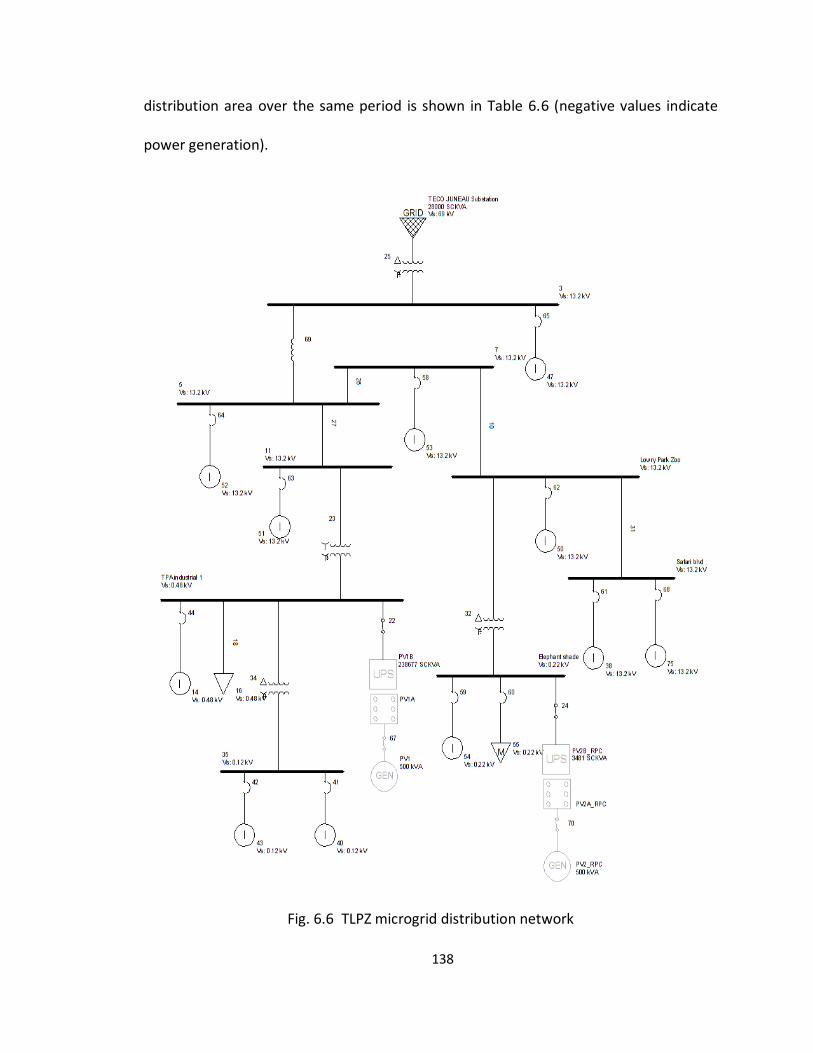
138
distribution area over the same period is shown in Table 6.6 (negative values indicate
power generation).
Fig. 6.6 TLPZ microgrid distribution network
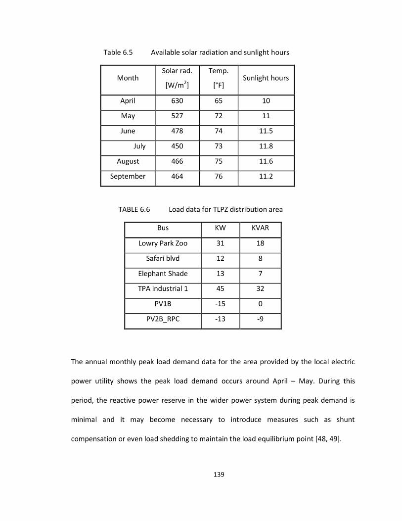
139
Table 6.5 Available solar radiation and sunlight hours
Month Solar rad.
[W/m2]
Temp.
[°F] Sunlight hours
April 630 65 10
May 527 72 11
June 478 74 11.5
July 450 73 11.8
August 466 75 11.6
September 464 76 11.2
TABLE 6.6 Load data for TLPZ distribution area
Bus KW KVAR
Lowry Park Zoo 31 18
Safari blvd 12 8
Elephant Shade 13 7
TPA industrial 1 45 32
PV1B -15 0
PV2B_RPC -13 -9
The annual monthly peak load demand data for the area provided by the local electric
power utility shows the peak load demand occurs around April – May. During this
period, the reactive power reserve in the wider power system during peak demand is
minimal and it may become necessary to introduce measures such as shunt
compensation or even load shedding to maintain the load equilibrium point [48, 49].
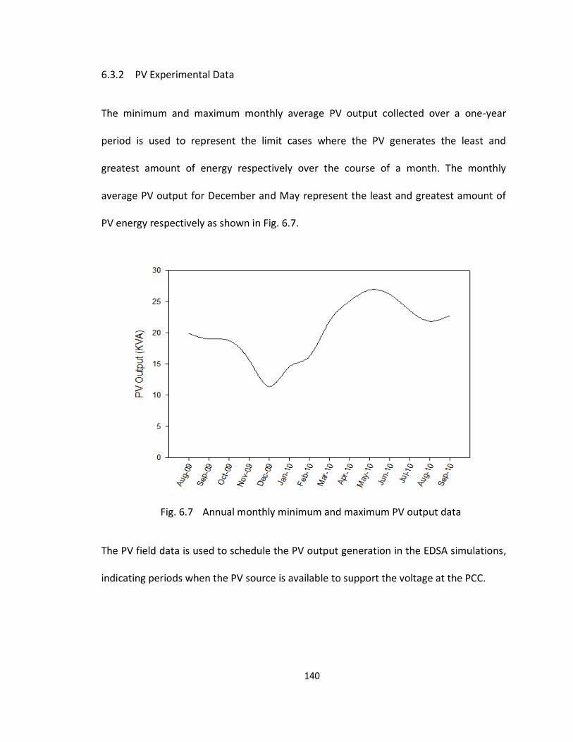
140
6.3.2 PV Experimental Data
The minimum and maximum monthly average PV output collected over a one-year
period is used to represent the limit cases where the PV generates the least and
greatest amount of energy respectively over the course of a month. The monthly
average PV output for December and May represent the least and greatest amount of
PV energy respectively as shown in Fig. 6.7.
Fig. 6.7 Annual monthly minimum and maximum PV output data
The PV field data is used to schedule the PV output generation in the EDSA simulations,
indicating periods when the PV source is available to support the voltage at the PCC.
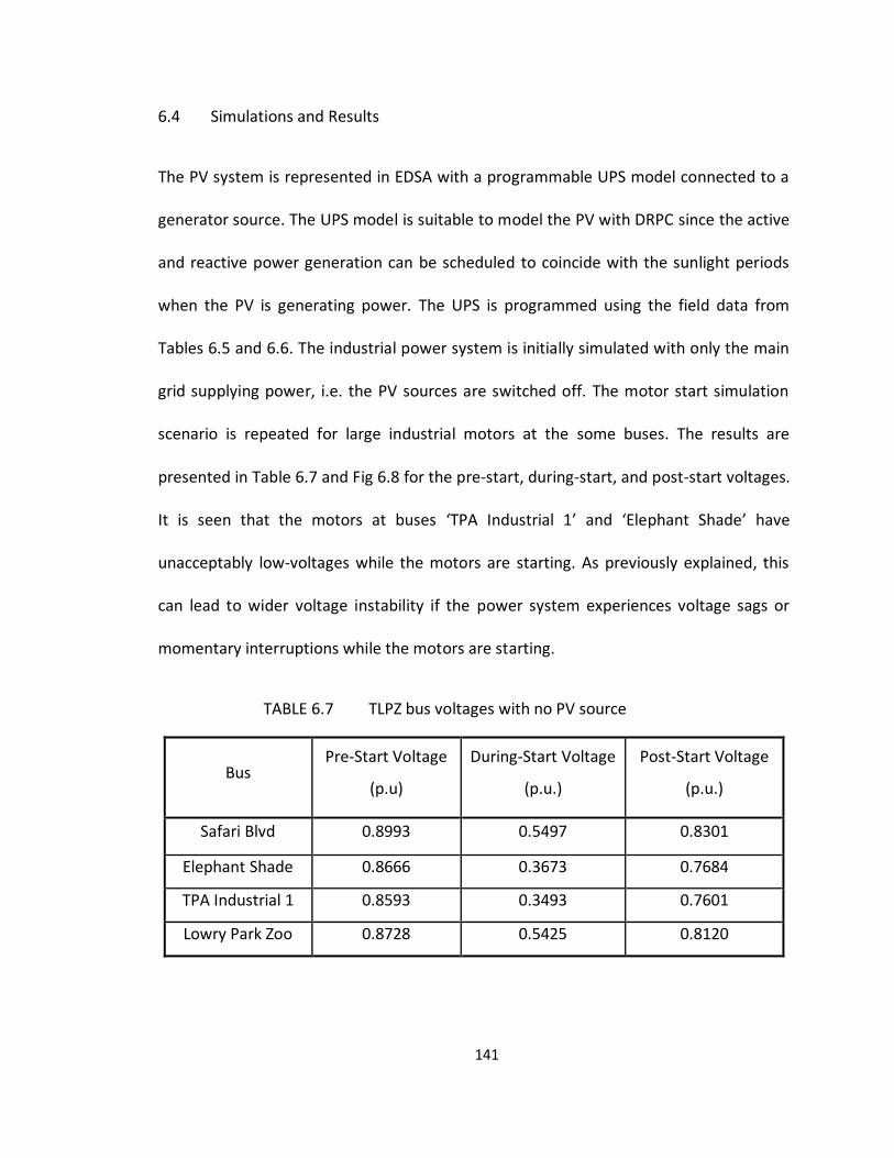
141
6.4 Simulations and Results
The PV system is represented in EDSA with a programmable UPS model connected to a
generator source. The UPS model is suitable to model the PV with DRPC since the active
and reactive power generation can be scheduled to coincide with the sunlight periods
when the PV is generating power. The UPS is programmed using the field data from
Tables 6.5 and 6.6. The industrial power system is initially simulated with only the main
grid supplying power, i.e. the PV sources are switched off. The motor start simulation
scenario is repeated for large industrial motors at the some buses. The results are
presented in Table 6.7 and Fig 6.8 for the pre-start, during-start, and post-start voltages.
It is seen that the motors at buses ‘TPA Industrial 1’ and ‘Elephant Shade’ have
unacceptably low-voltages while the motors are starting. As previously explained, this
can lead to wider voltage instability if the power system experiences voltage sags or
momentary interruptions while the motors are starting.
TABLE 6.7 TLPZ bus voltages with no PV source
Bus Pre-Start Voltage
(p.u)
During-Start Voltage
(p.u.)
Post-Start Voltage
(p.u.)
Safari Blvd 0.8993 0.5497 0.8301
Elephant Shade 0.8666 0.3673 0.7684
TPA Industrial 1 0.8593 0.3493 0.7601
Lowry Park Zoo 0.8728 0.5425 0.8120
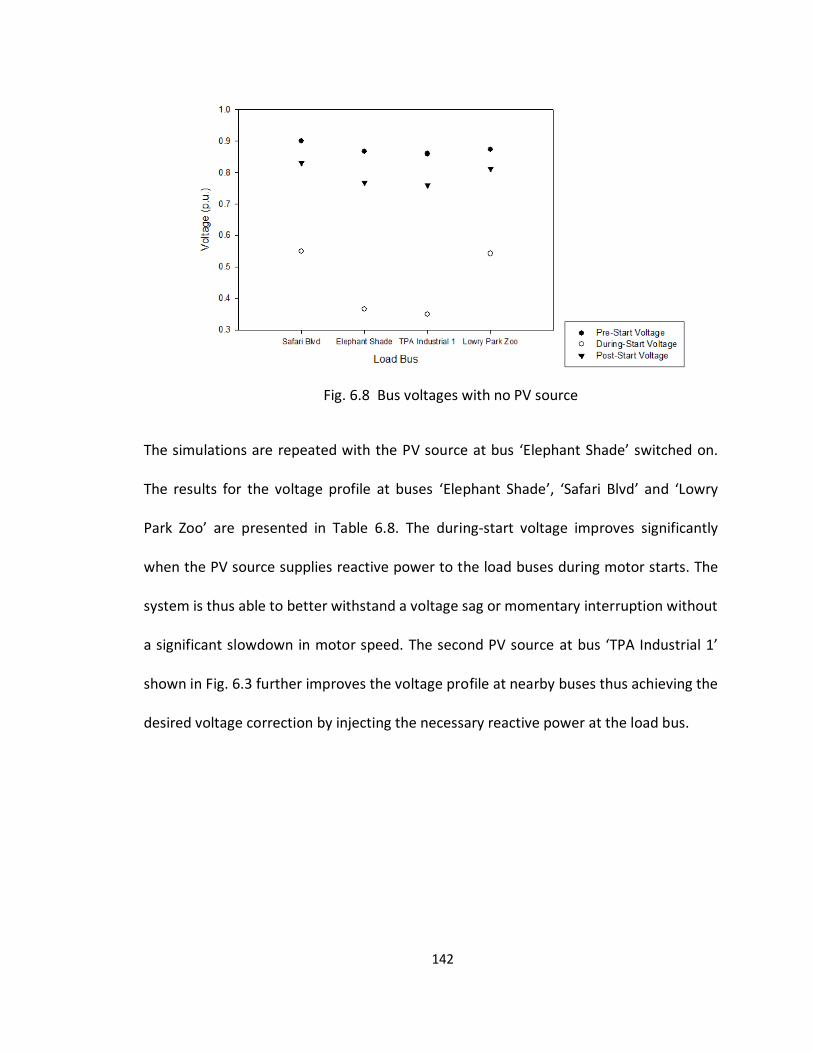
142
Fig. 6.8 Bus voltages with no PV source
The simulations are repeated with the PV source at bus ‘Elephant Shade’ switched on.
The results for the voltage profile at buses ‘Elephant Shade’, ‘Safari Blvd’ and ‘Lowry
Park Zoo’ are presented in Table 6.8. The during-start voltage improves significantly
when the PV source supplies reactive power to the load buses during motor starts. The
system is thus able to better withstand a voltage sag or momentary interruption without
a significant slowdown in motor speed. The second PV source at bus ‘TPA Industrial 1’
shown in Fig. 6.3 further improves the voltage profile at nearby buses thus achieving the
desired voltage correction by injecting the necessary reactive power at the load bus.
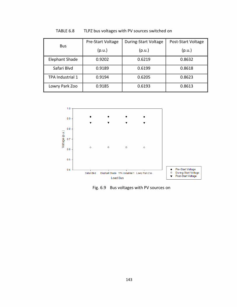
143
TABLE 6.8 TLPZ bus voltages with PV sources switched on
Bus Pre-Start Voltage
(p.u.)
During-Start Voltage
(p.u.)
Post-Start Voltage
(p.u.)
Elephant Shade 0.9202 0.6219 0.8632
Safari Blvd 0.9189 0.6199 0.8618
TPA Industrial 1 0.9194 0.6205 0.8623
Lowry Park Zoo 0.9185 0.6193 0.8613
Fig. 6.9 Bus voltages with PV sources on
144
7. CONCLUSIONS AND FUTURE WORK
The work has been focused on the following three issues related to distribution systems
with a high penetration of distributed generation: voltage stability, loadability limit
influence and dynamic reactive power control. An analytical method to determine the
voltage impact of DG sources at different locations in the power system based on the
size of the DG and adjacent loads, as well as remedial action if necessary, is presented.
The theory has been applied to a case study of the Tampa Lowry Park Zoo industrial
power system.
7.1 Conclusions
The impacts of adverse power quality issues on industrial loads have been presented
and different methods to classify the stability margin of an area EPS have been
illustrated with some simple examples. The four existing methods for voltage sag
mitigation – synchronous generator excitation control, shunt capacitor application, use
of FACTS devices, and LTC transformer adjustment – have been compared, and it is
found that synchronous generator excitation control is more suitable for voltage
regulation of large radial transmission systems than for DG-embedded distribution
145
systems. A new method for voltage sag mitigation based on dynamic reactive power
control of DGs has been presented. The method mitigates the transient impacts of static
on/off switching of passive reactive power compensation devices. The method also
improves the utilization factor of DGs that are already deployed in the power
distribution system by regulating the DGs to generate both active and reactive power
simultaneously. Utilities are thus able to achieve savings and minimize losses by
optimally deploying more flexible DGs into the distribution system instead of peaker
plants with low utilization factors. The method uses the same parameters that are used
to determine the voltage stability margin of any EPS excluding the contribution from
peaker plants or DGs. The maximum potential savings realizable is directly correlated
with the distance from the bifurcation point of the EPS with the exclusion of the peaker
plants. The impact of the method is greater on the short-term voltage stability, but for
relatively small systems, it can also improve the long-term voltage stability by increasing
the loadability limit of the power system.
The problem related to overvoltages at the PCC due to the presence of DGs in the power
distribution system has been examined. Simple expressions to determine the potential
voltage rise at the PCC as a result of DG current injection have been derived. For
photovoltaic sources, the PV current limit that is necessary to hold the voltage at the
PCC below a preset limit is determined based on the maximum capacity of the PV and
the distance from the substation. For PV sources operating at unity power factor in
industrial areas with a high concentration of induction motors, the local bus voltage rise
is found to be higher than for PV sources operating with a lagging power factor. This

146
represents a limiting factor in the maximum capacity of the PV plant. The network and
load characteristic of the power system are visualized using PV and QV curves, which
make it possible to study the corresponding effects of load shedding or varying either
the active power or the reactive power injection. This provides the utility a suitable
platform for design and planning practices.
7.2 Further Work
The application of the reactive power control method can be developed further by
including a central controller to autonomously regulate the power in multiple DG units.
The use of neural networks to train large autonomous systems can be useful for the
utility to balance the power flow in the power distribution system from the substation.
It will be interesting to investigate the interaction between the slow acting mechanical
devices of the synchronous generator and the fast acting devices of the power
electronics controllers when the system has to simultaneously respond to disturbances
occurring at more than one location.
147
REFERENCES
[1] Y. M. Atwa, E. F. El- Saadany, M. M. A. Salama, and R. Seethapathy, “Optimal renewable resources mix for distribution system energy loss minimization,” IEEE Transactions on Power Systems, Vol. 25, No. 1, Feb 2010.
[2] C. S. Chen, M. S. Kang, J. C. Hwang, and C. W. Huang, “Synthesis of power system load profiles by class load study,” International Journal of Electrical Power and Energy Systems, Vol. 22, No. 5, pp. 325-330, June 2000.
[3] A. J. Hoffman, “Peak demand control in commercial buildings with target peak adjustment based on load forecasting,” Proc. IEEE International Conference on Control Applications, Vol.2, pp 1292 - 1296, 1998.
[4] S. Rahman, J. Jockell, and S. Lahour, “Analysis of the value of photovoltaics for demand side management,” IEEE Photovoltaics Specialists Conference, Vol. 2, pp. 809 - 814, 1990.
[5] R. Wai and W. Wang, “Grid-connected photovoltaic generation systems,” IEEE Transactions on Circuits and Systems – 1: Regular Papers, Vol. 55, No. 3, April 2008.
[6] S. J. Huang and F. S. Pai, “Design and operation of grid-connected photovoltaic system with power-factor control and active islanding detection,” Proc. IEE Gen. Trans. Distrib., Vol. 148, No. 3, pp. 243 – 250.
[7] G. Petrone, G. Spagnuolo, Teodorescu, M. Veerachar, M. Vitelli, “Reliability issues in photovoltaic power processing systems,” IEEE Transactions on Industrial Electronics, Vol. 55, No. 7, July 2008.
[8] Y. Ueda, K. Kurokawa, T. Tanabe, K. Kitamura, S. Hiroyuki, “Analysis results of output power loss due to the grid voltage rise in grid-connected photovoltaic power generation systems,” IEEE Transactions on Industrial Electronics, Vol. 55, No. 7, July 2008.
[9] A. Martinez, H. Calleja, “A simple, high quality output PV system aimed at peak demand reduction,” IEEE International Power Electronics Congress, Mexico, 2000.
[10] J. C. Chow, R. Fischl, and H. Yan, “On the evaluation of voltage collapse criteria,” IEEE Transactions on power Systems, Vol. 5, No. 2, May 1990.
148
[11] N. Hosseinzadeh, “Power system blackouts: lessons learned,” Proc. of the Australasian Universities Power Engineering Conference, 2005.
[12] A. Domijan, “Power Con 2003- Special theme: blackout,” Proc. of the Ninth IASTED International conference, Dec 2003.
[13] A. Domijan, F. Torres, and C. Alvarez, “Microgrids: a look into the power delivery system of the future,” Proc. of the International Conference on Power and Energy Systems, Jan 2007.
[14] R. C. Dugan and T.E. Mc Dermott, “Operating conflicts for distributed generation on distributed systems,” Rural Electric Power Conference, 2001.
[15] S. Conti, S. Raiti, G. Ting, and U. Vagliasindi, “Study of the impact of PV generation on voltage profile in LV distribution networks,” IEEE Power Tech Proc., 2001.
[16] T. S. Basso and R. DeBlasio, “1547 series of standards: Interconnection issues,” IEEE Transactions on Power Electronics, Vol. 19, No. 5, pp. 1159 - 1162, 2004.
[17] S. Chaitusancy, A. Yokoyama, “Contribution of distributed generation to voltage regulation under stochastic attribute of renewable energy resources,” International Conference on Power System Technology, 2006.
[18] E. Liu and J. Bebic, “Distribution system voltage performance analysis for high- penetration photovoltaics,” National Renewable Energy Laboratory Report, Feb 2008.
[19] Y. Baghzouz, “Voltage regulation and overcurrent protection issues in distribution feeders with distributed generation – a case study,” Proc. of 38th Hawaii International Conference on System Sciences, 2005.
[20] G. Chicco, Giaccone, F. Spertino, G. Graditi, “Experimental methods to evaluate the impact of a photovoltaic system at the point-of-common coupling in low voltage networks,” International Symposium on Power Electronics, Electrical Drives, Automation and Motion, 2006.
[21] Y. Tachwali, H. Refai, and J. E. Fagan, “Minimizing HVAC energy consumption using a wireless sensor network,” 33rd Annual Conference of the IEEE Industrial Electronics Society, pp. 439 - 444, 2007.
[22] G. Crabtree, T. L. Jester, C. Fredric, J. Nickerson, V. Meemongokolkiat and A. Rohatgi, “Production viability of gallium doped mono-crystalline solar cells,” 31st IEEE Photovoltaic Specialist Conference, pp. 935 - 938, 2003.
149
[23] C. Sevik and C. Bulutay, “Gain and temporal response of AlGaN solar-blind avalanche photodiodes: An ensemble Monte Carlo analysis,” Applied Physics Letters, Vol. 83, No. 7, pp. 1382 - 1384, 2003.
[24] A. Omole, “Analysis, modeling and simulation of optimal power tracking of multiple-modules of paralleled solar cell systems,” Thesis Submitted to Electrical Engineering Dept. at Florida State University, Aug 2006.
[25] M. G. Villava, J. F. Gazoli, and E. R. Filho, “Comprehensive approach to modeling and simulation of photovoltaic arrays,” IEEE Transactions on Power Electronics, Vol. 25, No. 5, May 2009.
[26] T. Esram and P. L. Chapman, “Comparison of photovoltaic array maximum power point tracking techniques,” IEEE Transactions on Energy Conversion, Vol. 22, No. 2, pp. 435 - 449, 2007.
[27] T. Trupke, M. A. Green and P. Wurfel, “Improving solar cell efficiencies by down-conversion of high-energy photons,” Journal of Applied Physics, Vol. 92, No. 3, pp. 1668 - 1674, 2002.
[28] J. A. Gow and C. D. Manning, “Photovoltaic converter system suitable for use in small scale stand-alone or grid-connected applications,” IEEE Proceedings on Electric Power Applications, Vol. 82, No. 9, 1997.
[29] A. K. Newman and J. M. Liu, “Physical characteristics of band-gap engineered, photovoltaic detectors,” Journal of Applied Physics, Vol. 82, No. 9, 1997.
[30] E. Gholdston, J. Hartung, and J. Friefeld, “Current status, architecture, and future technologies for the international space station electric power system,” IEEE Aerospace and Electronic Systems Magazine, Vol. 11, No.2, pp. 25 – 30, 1996.
[31] B. Sahan, A. N. Vergara, N. Henze, A. Engler, and P. Zacharias, “ A single-stage PV module integrated converter based on a low-power current-source inverter,” IEEE Transactions on Industrial Electronics, Vol. 55, No. 7, pp. 2602 - 2609, 2008.
[32] J. M. Guerrero, J. Matas, L. Garcia de Vicuna, M. Castilla, and J. Mirer, “Decentralized control for parallel operation of distributed generation inverters using resistive output impedance,” IEEE Transactions on Industrial Electronics, Vol. 54, No. 2, pp. 994 - 1004, Apr 2007.
[33] P. G. Barbora, L. G. B. Rolin, E. H. Watanabe, and R. Hanitsch, “Control Strategy for grid-connected DC-AC converter with load power factor correction,” IEEE Proc. on Gen., Trans., and Dist., Vol. 145, No. 5, pp. 487 - 491, 2002.
150
[34] N. Mohan, T. M. Undeland, and W. Robbins, Power Electronics: Converters, Applications and Design, Wiley & Sons, 2003.
[35] J. T. Bialasiewicz, “Renewable energy systems with photovoltaic power generators: Operation and modeling,” IEEE Transactions on Industrial Electronics, Vol. 55, No. 7, pp. 2752 - 2758, 2008.
[36] Y. T. Tan, D. S. Krischen, and N. Jenkins, “A model of PV generation suitable for stability analysis,” IEEE Transactions on Energy Conversion, Vol. 19, No. 4, Dec. 2004.
[37] P. Kundur, Power System Stability and control, McGraw-Hill Inc., New York, 1994.
[38] J. J. Grainger and W. D. Stevenson, Power System Analysis, McGraw-Hill Inc., New York, 1968.
[39] M. LaScala, G. Lorusso, R. Sbrizzai, M. Trovato, “A qualitative approach to the transient analysis of power systems,” IEEE Transactions on Power Systems, Vol. 11, No. 4, pp. 1996 - 2002, 1996.
[40] J. A. Momoh, Y. V. Makarov, W. Mittelstadt, “A framework of voltage stability assessment in power system reliability analysis,” IEEE Transactions on Power Systems, Vol. 14, No. 2, pp. 484 - 491, 1999.
[41] M. H. J. Bollen, Understanding Power Quality Problems, John Wiley and Sons Inc., New Jersey, 2000.
[42] K. H. La Commare and J. H. Eto, “Understanding the cost of power interruptions to US electricity customers,” Report No. LBNL-55718, Berkeley, California: Lawrence Berkley National Laboratory, 2004.
[43] Z. Lidong and M. H. J. Bollen, “Characteristic of voltage dips (sags) in power systems,” IEEE Transactions on Power Delivery, Vol. 15, No. 2, 2000.
[44] P. Heine and M. Lehtonen, “Voltage sag distributions caused by power system faults,” IEEE transactions on Power Systems, Vol. 18, No. 4, pp. 1367 - 1373, 2003.
[45] Review of Florida’s investor-owned electric utilities’ service reliability on 2008, Florida Public Service Commission, Dec 2009.
[46] Z. F. Hussien, A. B. Ismail, W. C. Lee, A. M. Busrah, and M. F. M. Siam, “Voltage sag mitigation using NAS battery-based standby power supply,” International Conference on Power Electronics and Drives Systems, Vol. 2, pp. 1317 – 1321, 2005.
[47] A. Wiszniewski, “ New criteria of voltage stability margin for the purpose of load shedding,” IEEE transactions on Power Delivery, Vol.22, No.3, pp 1367-1371, 2007
151
[48] A. Ghosh and D. Chatterjee, “Transient stability assessment of power systems containing series and shunt compensators,” IEEE Transactions on Power Systems, Vol. 22, No. 3, pp. 1210 – 1220, 2007.
[49] H. F. Wang, H. Li, and H. Chen, “Coordinated secondary voltage control to eliminate voltage violations in power system contingencies,” IEEE Transactions on Power Systems, Vol. 18, No. 2, pp. 588 – 595, 2003.
[50] L. Camilo, J. C. Cebrian, N. Kagan, and N. M. Matsuo, “Impact of distributed generation units on the sensitivity of customers to voltage sags,” International Conference and Exhibition on Electricity Distribution, pp. 1 - 4, 2005.
[51] B. Renders, K. De Gusseme, W. R. Ryckaert, K. Stockman, L. Vandevelde, M. H. J. Bollen,” Distributed generation for mitigating voltage dips in low-voltage distribution grids,” IEEE Transactions on Power Delivery, Vol. 23, No. 3, pp. 1581 - 1588, 2008.
[52] B. Renders, W. R. Ryckaert, K. De Gusseme, K. Stockman, and L. Vandevelde, “Improving the voltage dip immunity of converter-connected distributed generation units," Elsevier Renewable Energy, Vol. 33, No. 5, pp. 1011 - 1018, May 2008.
[53] E. G. Potamianakis and C. D. Vournas, “Short-term voltage instability: effects on synchronous and induction machines,” IEEE Transactions on Power Systems, Vol. 21, No. 791 – 798, 2006.
[54] T. V. Cutsem and C. Vournas, Voltage Stability of Electric Power Systems, Springer LLC, New York, 2008.
[55] IEEE Task Force on Excitation Limiters, “Recommended models for excitation limiting devices,” IEEE Transactions on Energy Conversion, 1996.
[56] M. Reza, “Stability analysis of transmission systems with high penetration of distribution generation,” Dissertation submitted to the Delft University of Technology, Dec 2006.
[57] U. R. Pthula, Static and Dynamic Voltage Stability Analysis, Lambert AG & Co., Saarbrücken, 2010.
[58] A. Sallam, M. Desouky, and H. Desouky, “Shunt capacitor effect on electrical distribution system reliability,” IEEE Transactions on Power systems, Vol. 43, No. 1, pp. 170 - 176, 1994.
[59] E. Zhou, “Application of static VAr compensators to increase power system damping,” IEEE Transactions on Power Systems, Vol. 8, No. 2, pp. 655 - 661, 1993.
152
[60] R. H. Liang and C. K. Cheng, “ Dispatch of a main transformer ULTC and capacitors in a distribution system,” IEEE Power Engineering Review, Vol. 21, No. 7, 2001
[61] S. Alepuz, S. Busquets-Monge, J. Bordonau, J. Gago, D. Gonzalez, J. Balcells,
“Interfacing renewable energy sources to the utility grid using a three-level
inverter,” IEEE Transactions on Industrial Electronics, Vol. 53, No. 5, pp. 1504 –
1511, 2006.
[62] E. Paraskevadaki, S. Papathamassion, and M. Papadopoulos, “Benefits from DG power factor regulation in LV networks,” 20th CIRED International Conference and Exhibition on Electricity Distribution - Part 1, pp. 1 - 4, 2009.
[63] Y. A. Mohamed and E. F. El-Saadany, “A control method of grid-connected PWM voltage source inverters to mitigate fast voltage disturbances,” IEEE Transactions on Power Systems, Vol. 24, No. 1, pp. 489 - 491, 2009.
[64] H. M. Ayres, W. Freitias, M. C. De Almedia and L. C. P. Da Silva, “ Method for determining the maximum allowable penetration level of distributed generation without steady-state voltage violations,” IET Generation, Transmission and Distribution, Vol. 4, No. 4, pp. 495 - 508, 2010
[65] L. Castaner and S. Silvestre, Modeling Photovoltaic systems using PSpice, Wiley Inc., Sussex, 2002.
[66] R. Benato and R. Caldon, “Distribution line carrier: analysis procedure and application to DG,” IEEE Transactions on Power Delivery, Vol. 22, No. 1, 2007.
[67] P. Chiradeja,” Benefit of distributed generation: A line loss reduction analysis,” IEEE/ PES Asia and Pacific Transmission and Distribution Conference, 2005.
[68] P. Chiradeja and R. Ramakumar,” An approach to quantify the technical benefits of distributed generation,” IEEE Transactions on Energy Conversion, pp. 764 - 773, 2004.
[69] R. Brundlinger and B. Bletterie, “Unintentional islanding in distribution grids with a high penetration of inverter-based DG: Probability for islanding and protection methods,” IEEE Power Tech Conference, 2005
[70] R. A. Walling and N. W. Miller, “Distributed generation islanding – implications on power system dynamic performance, “IEEE Power Engineering Society Meeting, Vol. 1, pp. 92 – 96, 2002.
[71] A. Woyte, R. Belmans, and J. Nijs, “Testing the islanding protection function of photovoltaic inverters,” IEEE Transactions on Energy Conversion, Vol. 18, No. 1, pp. 157 – 162, Mar 2003.
153
[72] V. John, Y. Zhihong, and A. Kolwalkar, “Investigation of anti-islanding protection of power converter based distributed generators using frequency domain analysis,” IEEE Transactions on Power Systems, Vol. 19, No. 5, 2004.
[73] G. Yalcinkaya, M.H.J. Bollen, and P.A. Crossley, “Characterization of voltage sags in industrial distribution systems,” IEEE Transactions on Industry Applications, Vol. 34, No. 4, July/Aug 1998.
[74] M. H. J. Bollen, “The influence of motor reacceleration on voltage sags,” IEEE Transactions on Industrial Applications, Vol. 31, pp. 667 – 674, July/Aug 1995.
[75] R. E. Fehr, “Industrial Power Distribution,” New Jersey: Prentice-Hall, 2002.
[76] S. A. M. Javadian, A. M. Nasrabadi, M. R. Haghiform, and J. Rezvantalab, “Determining fault’s type and accurate location in distribution systems with DG using MLP neural networks,” International Conference on Clean Electrical Power, pp. 284 - 289, 2009.
[77] A. Canova, L. Giaccone, F. Spertino, M. Tartaglia, “Electrical impact of photovoltaic plant in distributed network,” IEEE Transactions on Industry Applications, Vol. 45, No. 1, Jan/Feb 2009
[78] B. H. Lee and K. Y. Lee, “Dynamic and static voltage stability enhancement of power systems,” IEEE transactions on Power Systems, Vol. 8, No. 1, pp. 231 - 238, 1993.
[79] J. C. Das, “Effects of momentary voltage dips on the operation of induction and synchronous motors,” IEEE Transactions on Industry Applications, Vol. 26, No. 4, pp. 711 – 718, 2004.
[80] A. Trzynadlowski, Control of Induction Motors, Academic Press, San Diego, 2001.
[81] IEEE Task Force on Load Representation for Dynamic Performance, “Standard load models for power flow and dynamic performance simulation,” IEEE transactions on Power Systems, Vol. 10, No. 3, pp. 1302 – 1312, Aug 1995.
[82] C. W. Taylor, Power System Voltage Stability, McGraw-Hill, 1994.
[83] G. Tzong-Tih and R. A. Schlueter, “Identification of generic bifurcation and stability problems in power system differential- algebraic model,” IEEE Transactions on Power Systems, pp. 1032 - 1044, 1994.
[84] R. Seydel, Practical Bifurcation and Stability Analysis (Inter-disciplinary Applied Mathematics), Springer LLC, New York, 2010.
154
[85] I. Dobson and L. Lu, “ New methods for computing a closest saddle node bifurcation and worst case load power margin for voltage collapse,” IEEE Transactions on Power Systems, Vol. 8, No. 3, pp. 905 - 913, 1993.
[86] L. Qi, “AC system stability analysis and assessment for shipboard power systems,” A Dissertation submitted to the Electrical Engineering Dept., Texas A &M University, Dec 2004.
[87] M. Jazaeri and M. Khatibi, “A study on Hopf bifurcations for power system stability analysis,” IEEE Electric Power Conference, pp. 1 - 6, 2008.
[88] J. Xia and M. Xin, “Bifurcation analysis for power system voltage stability based on singular perturbation method,” International Conference on Electrical Machines and Systems, pp. 1811 - 1814, 2007.
[89] G. C. Pyo, H. W. Kang, and S. I. Moon, “A new operation method for grid-connected PV system considering voltage regulation in distribution system,” IEEE Power and Energy Society General Meeting – Conversion and Delivery of Electrical Energy in the 21st Century, Vol. 1, pp. 1 – 7, 2008.
[90] IEEE PES Distribution Test Feeder Working Group, “Distribution test feeders,” IEEE PES Distribution System Analysis Subcommittee, Winter Power Meeting, 1991.

155
APPENDIX A: PICTURE OF LOWRY PARK ZOO PV INSTALLATION
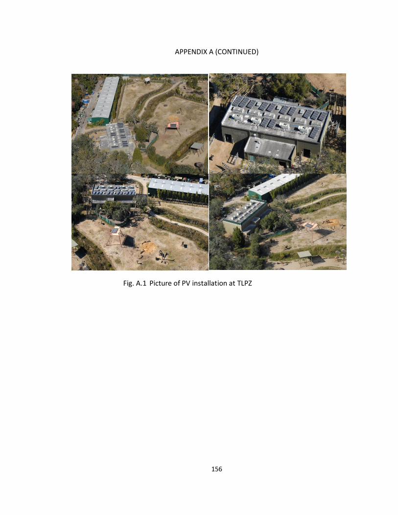
156
APPENDIX A (CONTINUED)
Fig. A.1 Picture of PV installation at TLPZ