Parametric Stability Assessment of Single-phase Grid-tied ...

General rights Copyright and moral rights for the publications made accessible in the public portal are retained by the authors and/or other copyright owners and it is a condition of accessing publications that users recognise and abide by the legal requirements associated with these rights.

Users may download and print one copy of any publication from the public portal for the purpose of private study or research.

You may not further distribute the material or use it for any profit-making activity or commercial gain

You may freely distribute the URL identifying the publication in the public portal If you believe that this document breaches copyright please contact us providing details, and we will remove access to the work immediately and investigate your claim.

Downloaded from orbit.dtu.dk on: Jul 08, 2022

Parametric Stability Assessment of Single-phase Grid-tied VSCs Using Peak andAverage dc Voltage Control

Zhang, Chen; Isobe, Takanori; Suul, Jon Are; Dragicevic, Tomislav; Molinas, Marta

Published in:IEEE Transactions on Industrial Electronics

Link to article, DOI:10.1109/TIE.2021.3068551

Publication date:2021

Document VersionPeer reviewed version

Link back to DTU Orbit

Citation (APA):Zhang, C., Isobe, T., Suul, J. A., Dragicevic, T., & Molinas, M. (2021). Parametric Stability Assessment of Single-phase Grid-tied VSCs Using Peak and Average dc Voltage Control. IEEE Transactions on Industrial Electronics,69(3), 2904 - 2915. https://doi.org/10.1109/TIE.2021.3068551

https://doi.org/10.1109/TIE.2021.3068551

https://orbit.dtu.dk/en/publications/e3dd0a90-5c08-4946-823c-e2644ee2ad87

https://doi.org/10.1109/TIE.2021.3068551

0278-0046 (c) 2021 IEEE. Personal use is permitted, but republication/redistribution requires IEEE permission. See http://www.ieee.org/publications_standards/publications/rights/index.html for more information.

This article has been accepted for publication in a future issue of this journal, but has not been fully edited. Content may change prior to final publication. Citation information: DOI 10.1109/TIE.2021.3068551, IEEETransactions on Industrial Electronics

IEEE TRANSACTIONS ON INDUSTRIAL ELECTRONICS

Abstract—A type of peak-value dc voltage control (denoted as PK control) was proposed in the literature for supporting the use of a smaller dc-side capacitance when the single-phase Voltage Source Converter (VSC) is operated as a Static Synchronous Compensator (STATCOM). Although it was demonstrated to operate stably under several conditions, it will be revealed in this paper how the PK control will suffer from a more severe small-signal stability issue under non-ideal grid conditions than the conventional method of controlling the average-value of the dc voltage (denoted as Avr control). Especially, it will be shown how the PK control is sensitive to some of the control parameters. To obtain these results, a parameter-oriented stability analysis method is developed in the linear-time periodic (LTP) framework. Then, it is utilized for parametric stability assessments of the Avr and PK control. Finally, both frequency- and time-domain experimental results verified the effectiveness and accuracy of the applied method in the presented analysis.

Index Terms—dc voltage control, LTP, small-signal modeling, stability, STATCOM, VSC

I. INTRODUCTION

ECENT experience in operating wind farms [1] and

photovoltaic (PV) power plants [2] have shown that

Voltage Source Converters (VSCs) are prone to small-

signal instability when connected to weak grids. Numerous

works have been conducted in this respect using the impedance-

based approach [3]-[5], and a variety of VSC impedance

models have been proposed [6]-[11]. Such models have served

not only for stability analysis but also for revealing the

frequency-domain characteristics of VSCs, e.g., the frequency

coupling effects [9], [10], and the properties of dq (a)symmetry

[12], [13]. Although these earlier works are useful for

understanding various stability issues of VSC, most of them are

fulfilled in the linear time-invariant (LTI) framework, where the

system’s steady-state is assumed to be time-invariant and

constant. The premise of a time-invariant representation is hard

to achieve for many converter systems, including single-phase

VSCs, in which the system’s steady-state is generally

This work is supported by Energy Technology Development and Demonstration Program (EUDP) (ACTION project, grant No. 56537).

C. Zhang and T. Dragičević are with the Department of Electrical Engineering, Technical University of Denmark (DTU), Denmark, (email: [email protected]; [email protected]).

T. Isobe is with the Faculty of Pure and Applied Sciences, University of Tsukuba, Japan (email: [email protected]).

characterized by periodic trajectories, i.e., depending on a

periodic steady-state (PSS) system representation.

To cope with the modeling and analysis of PSS systems, the

linear time-periodic (LTP) method [14], [15] can be applied. An

early but heuristic application of the method in identifying and

analyzing the harmonic interaction of converters in electrical

railways was presented in [16]. Lately, this method has become

appealing for modeling and stability analysis of converters with

inherent PSS characteristics, e.g., the modular multilevel

converters (MMCs) [17], [18], and the single-phase VSCs [19].

Despite the superior applicability of the LTP method, it is not

as easy to apply as the LTI method. Hence, in many cases, the

LTI method is still attractive when the time varying effects are

not evident or can be neglected under certain conditions. E.g.,

if the double grid-frequency oscillations in the dc voltage of a

single-phase VSC system is small [20], it can be modeled

similarly as the three-phase VSC using the LTI method [20]-

[23]. However, this simplification may lead to inaccurate

results when the PSS effect is substantial [24], e.g., the single-

phase VSC equipped with a small dc-side capacitor, which is

the scenario considered for the analysis presented in this work.

This paper is addressing the stability analysis and

comparison of two types of dc voltage control strategies applied

to a single-phase grid-tied VSC operated as a Static

Synchronous Compensator (STATCOM). In this application,

the peak-value of the dc-side capacitor voltage will be

synchronized with the peak value of the maximum required ac-

side output voltage when the converter is injecting reactive

power to the grid [25]. This allows for operating the single-

phase STATCOM with reduced dc-side capacitance and

correspondingly larger double grid-frequency oscillations of

the dc voltage without increasing the peak value of the capacitor

voltage. However, an explicit estimation and control of the

peak-value of dc voltage is required, rather than the commonly

applied approach of controlling the average value of the dc

voltage [21] (denoted as “Avr control” for brevity). For this

purpose, [26] presented a second-order generalized-integrator

(SOGI)-based filter for estimating the peak-value of the dc

voltage. The resulting dc voltage control scheme is briefly

denoted by “PK control” in later analysis.

J. A. Suul is with SINTEF Energy Research, also with the Department of Engineering Cybernetics, Norwegian University of Science and Technology (NTNU), Norway (e-mail: [email protected]).

M. Molinas is with the Department of Engineering Cybernetics, NTNU, Norway (email: [email protected])

Chen Zhang, Takanori Isobe, Jon Are Suul, Tomislav Dragičević and Marta Molinas

Parametric Stability Assessment of Single-phase Grid-tied VSCs Using Peak and

Average dc Voltage Control

R

Authorized licensed use limited to: Danmarks Tekniske Informationscenter. Downloaded on April 05,2021 at 16:36:14 UTC from IEEE Xplore. Restrictions apply.

mailto:[email protected]








Although the PK control introduced in [26] was shown to

operate stably with a small dc-side capacitance, the result was

obtained under ideal grid conditions. As will be revealed in this

paper, the PK control will suffer from a more limited stability

range under non-ideal grids than the Avr control. Therefore,

aside from the above-mentioned merits of PK control in

enabling operation with reduced dc-side capacitance, an in-

depth evaluation of PK control in view of stability is desired.

To this end, this paper will contribute to the following aspects:

1) Developing a parameter-oriented stability assessment

method in the LTP framework, which will serve as a tool for

fast and efficient parametric stability assessment of this paper.

2) Revealing and discussing the potential stability issues

of the PK control provoked by non-ideal grid conditions.

3) Comparing and clarifying the stability performance of

the Avr and PK control over a wide parameter space.

II. PARAMETER-ORIENTED STABILITY ANALYSIS METHOD

APPLIED TO THE SINGLE-PHASE GRID-VSC SYSTEM

A. Study system

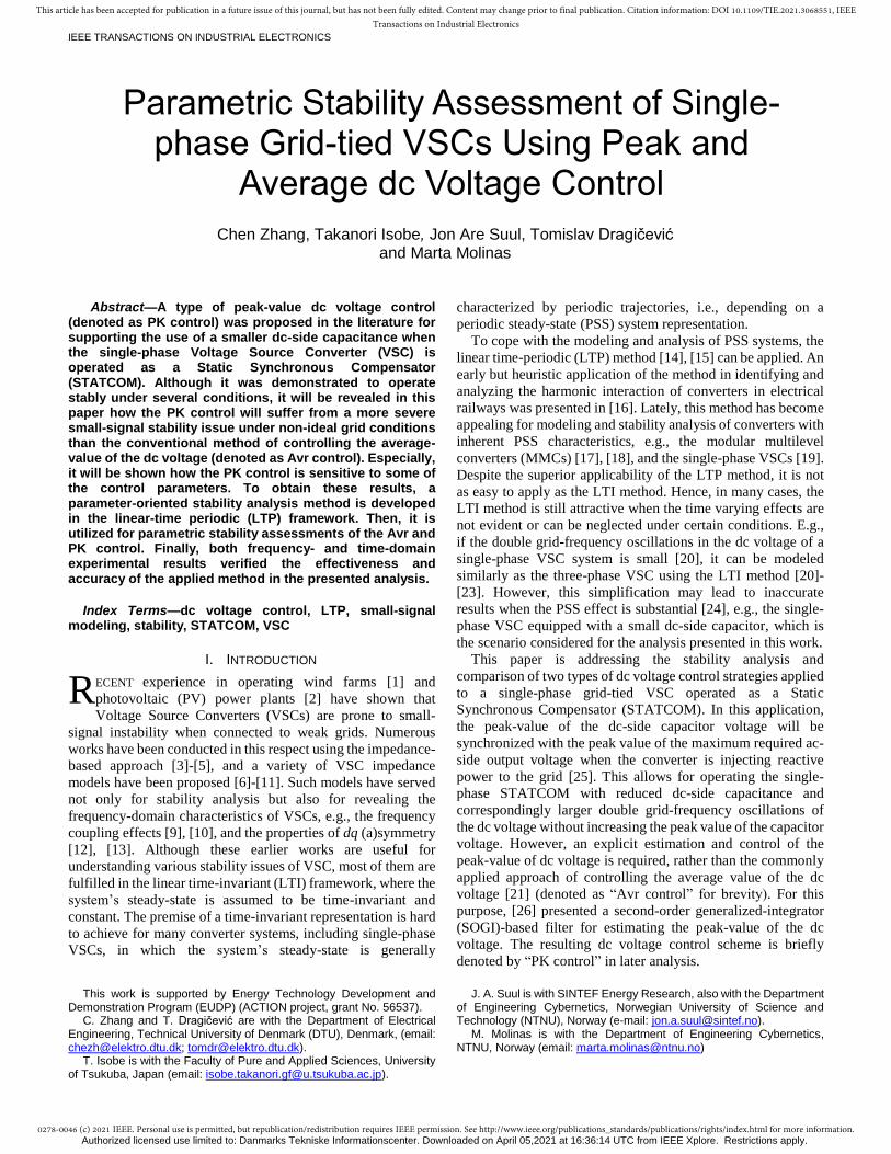
As shown in Fig. 1 (a), the control system of the single-phase

STATCOM mainly consists of: the proportional resonant (PR)-

based current controller, the proportional integrator (PI)-based

dc voltage controller, and the grid-synchronization unit. The

synchronization strategy is relying on a SOGI-based

Quadrature Signal Generator (QSG) and a Synchronous

Reference Frame (SRF) phase-locked-loop (PLL). Detailed

information on the control blocks is given in Fig. 1 (b). The

aforementioned dc voltage control strategies are listed below:

1) the Avr control, where the square of the measured dc

voltage 2dcu t is directly regulated, as shown in Fig. 1 (a);

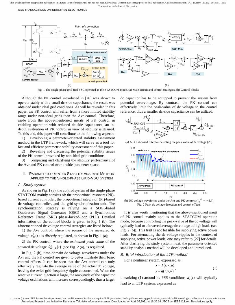
2) the PK control, where the estimated peak value of the

squared dc voltage 2dc_pku t (see Fig. 2 (a)) is regulated.

In Fig. 2 (b), time-domain dc voltage waveforms under the

Avr and the PK control are given to better illustrate their basic

control effects. It can be seen that the Avr control can only

effectively regulate the average value of the actual dc voltage,

leaving the twice grid-frequency ripple uncontrolled. When the

reactive current injection is large, the amplitude of the capacitor

voltage oscillations will increase correspondingly, thus a larger

dc capacitor has to be equipped to prevent the system from

potential overvoltage. By contrast, the PK control can

effectively limit the peak-value of dc voltage to the control

reference, thus a smaller dc-side capacitance can be utilized.

2

2

𝑘𝑠𝑜𝑔𝑖 _𝑑𝑐

𝑢𝑑𝑐2

2𝜔1

𝑢𝑑𝑐 _𝛼2

𝑢𝑑𝑐 _𝛽2

𝑢 𝑑𝑐2

𝑢 𝑑𝑐2𝜔_𝑝𝑘2

𝑢 𝑑𝑐 _𝑝𝑘2

(𝑘𝑠𝑜𝑔𝑖_𝑑𝑐 )

SOGI-QSG

(a) A SOGI-based filter for detecting the peak value of dc voltage [26]

(b) DC voltage waveforms under the Avr and PK controls (𝑖𝑞

𝑟𝑒𝑓= −3𝐴)

Fig. 2 Peak dc voltage detection and control effects

It is also worth mentioning that the above-mentioned merit

of PK control mainly applies to the STATCOM operation

mode, because controlling the peak-value of the dc voltage will

typically lead to a lowered average dc voltage at high loads (see

Fig. 2 (b)). This trait is not feasible for supplying active power

loads. For attenuating the dc voltage ripples in the context of

supplying active power loads, one may refer to [27] for details.

After clarifying the study system, next, the parameter-oriented

stability analysis method will be developed and introduced.

B. Brief introduction of the LTP method

For a nonlinear system, expressed as

, ,

, ,

t

t

x f x u

y g x u, (1)

linearizing (1) around its PSS conditions 0 tx will typically

lead to an LTP system, expressed as

Q1

Q2

Q3

Q4

Point of connection (PoC)

cos

sin

HPR

Current control

𝑅𝑓 𝑅𝑔 𝐿𝑓 𝐿𝑔

𝑢𝑔 𝑢𝑎

𝑖𝑑𝑐

𝑢𝑑𝑐 𝐶𝑐𝑎𝑝

𝑸1−4

𝑖𝑎

𝑖𝑞𝑟𝑒𝑓

𝑖𝑎𝑟𝑒𝑓

𝑖𝑎

𝑚𝑎𝑟𝑒𝑓

𝑢𝑎𝑟𝑒𝑓

𝑢𝑑𝑐 Hdc

𝑢𝑑𝑐2 𝑖𝑑

𝑟𝑒𝑓

𝑉𝑑𝑐 _𝑟𝑒𝑓2

𝑢 𝑑𝑐 _𝑝𝑘2

Avr:

PK:

SOGI-QSG

SRF-PLL

Synchronization unit

𝜃𝑝𝑙𝑙 𝑢 𝑎

𝑢 𝑏

𝑢𝑎

Control mode

dc voltage control

SPWM

𝑥𝑑𝑐

𝑘𝑝𝑑𝑐

𝑘𝑖𝑑𝑐 𝑥𝑝𝑙𝑙

𝑘𝑝𝑝𝑙𝑙

𝑘𝑖𝑝𝑙𝑙

Hdc Hpll

SOGI-QSG

𝑢𝑎 𝑘𝑠𝑜𝑔𝑖

𝜔1 𝑢 𝑎

𝑢 𝑏

𝑥𝑠𝑜𝑔𝑖𝑏

𝑥𝑠𝑜𝑔𝑖𝑎

SRF-PLL

𝜃𝑝𝑙𝑙 𝜔1 𝑢𝑑

𝑢𝑞

𝛼𝛽/𝑑𝑞 𝐻𝑝𝑙𝑙

𝑢 𝑎

𝑢 𝑏

HPR

𝜔1

2𝑘𝑖𝑐

𝜔1

𝑥𝑝𝑟𝑎

𝑥𝑝𝑟𝑏 𝑘𝑝𝑐

(a) (b)

Fig. 1 The single-phase grid-tied VSC operated as the STATCOM mode. (a) Main circuit and control strategies. (b) Control blocks





A t B t

C t D t

x x u

y x u (2)

where 0 tA t

x

f

x, 0 tB t

u

f

u, 0 tC t

x

g

x, and

0 tD t

u

g

u, while 0 tu is the system’s steady-state input

vector. Stability analysis of (2) can be typically performed in

two ways: 1) use of the Floquet theory [14], where the

eigenvalue of a so-called monodromy matrix obtained from a T-

period numeric integration of tA is analyzed; 2) apply the

Hill’s frequency-domain method [14], where the eigenvalue of

a so-called harmonic-state-space (HSS) model expressed by (3)

is evaluated (i.e., the eigenvalues of the matrix blk ) [19].

blk

(3)

where blk 1 1j ,...,0,..., jdiag k k I I is a block diagonal

matrix; 1 is the fundamental frequency; I is an identity

matrix with the same dimension as the state vector x ;

,k N N is defined for numeric implementation, and N is the

highest harmonic-order (its value will be discussed later).

, , are spectral vectors collecting the Fourier

coefficients of vectors , , x u y , e.g.,

0,..., ,...,T

k k X X X and the element kX denotes the k-

th Fourier coefficient of x . This definition also applies to

and . At last, , , , are Toeplitz formatted matrices of

, , ,A t B t C t D t .

It should be noted that both methods rely on the knowledge

of 0 tx or its Fourier coefficients . This means that the PSS

conditions should be obtained beforehand, which is usually

assisted by time-domain simulations, i.e., via numeric

integration of the system (1). However, the simulation-based

PSS extraction method has two main drawbacks when applied

to parametric studies: 1) changing the system’s parameters will

typically lead to a new set of PSS conditions, which need to be

updated by running a new simulation and the process of which

is time-consuming; 2) by running the simulation, only the stable

PSS conditions can be extracted. This restricts its application in

parametric stability analysis when the parameters should be

swept over wide ranges which likely result in the presence of

unstable PSS conditions. To overcome these issues and achieve

a fast and efficient PSS extraction, the frequency-domain

iteration-based approach described in [28] could be adopted.

C. The iteration-based PSS extraction method

First, from (1), the i-th iterative model can be written as:

, ,i i i i i i

i it

f fx x f x u x u

x u (4)

where

i

iA t

f

x and

i

iB t

f

u . For PSS calculation,

(4) represents a closed-loop system, where iu is an input

vector consisting of the system’s time-invariant parameters, e.g.,

control references, control parameters, and the magnitude and

phase of the supplying source voltage. Since iu is known and

fixed during the iteration, the last term can be omitted.

Transforming (4) into the frequency-domain and applying

the principle of harmonic balance, the i-th iterative model for

the k-th harmonic can be obtained as:

( )

blk

ii i iik m mk k k

m

X X F A X (5)

where ikX denotes the k-th Fourier coefficient of x at the i-th

step, and ( ) ii

k kF f . The operator

k is to extract the k-th

Fourier component of a periodically time-varying function.

Finally, applying (5) to each harmonic and collecting the

resulting equations will lead to the final frequency-domain

iteration model that can be compactly written as:

1

blk blk

1

i i i i

i i i

(6)

where 0,..., ,...,Ti

k k F F F is the collection of Fourier

coefficients of , ,i i

tf x u . To solve (6) numerically, the

upper boundary of ,k N N should be determined. In

principle, the higher the N the better the precision. However, a

large N is computationally expensive and usually not necessary.

E.g., since this paper applies the principle of switching-average

for modeling the VSC system, the modelled system will be free

from switching and sideband harmonics, thus a relatively low

N can be considered. In this work, N = 4 is applied and its

validity will be verified by experiments later. Once N is

determined, generally, (6) can be solved by iterations (e.g., the

Newton’s method) until a pre-defined tolerance is reached.

Next, this method will be implemented in MATLAB for

parametric stability analysis. The resulting algorithm will

contain three main parts: 1) the model preparation subroutine;

2) the numeric iteration subroutine, and 3) the main routine for

parameter sweeps. They will be elaborated below.

D. Algorithmic implementation of the method for parametric stability analysis

1) The model preparation subroutine To achieve a tool that is easy and efficient to apply, the

system modeling is automatized by using symbolic calculations

of MATLAB, where the following steps will take place to

obtain all the necessary time-domain functions for study:

First, define and formulate the closed-loop system model (1)

using the command syms (). Then, perform a system-wide

linearization on (1) using the command jacobian(), so that

, , ,A t B t C t D t are further obtained. Finally,

parameterize these functions using the command

matlabFunction () for better numeric performance when

interfacing them with the next subroutine. It is also worth

mentioning that, for this work, this subroutine only needs to be

run once as the structure of the system is fixed.

2) The numeric iteration subroutine This subroutine aims to solve (6) using Newton’s method.

However, from the above analysis, it can be seen that solving

(6) requires time-frequency domain transformation of variables

and functions. For which, numerical evaluation of those time-





domain functions with a duration of Teval (i.e., usually set as the

system’ period) and a time-step heval will be executed internally.

The detailed steps fulfilling this subroutine include:

Step 1: Numerical evaluation of functions (e.g., iA t with

Teval and heval) using a previously obtained ix (or initial states);

Step 2: Transform the results into frequency-domain and

collect , ,

i i i for updating 1i i

according to

(6). Afterward, apply the inverse Fourier transform to find 1i

x , preparing for the next iteration;

Step 3: If i is met, exit and output i (or

0

it x x ); otherwise, go to Step 1. It should be noted that the

outputs of the process also include useful by-products for LTP

analyses, e.g., i is used for later stability analysis, while

, , ,

i i i i are relevant matrices for generating the

VSC’s impedance, which will be shown in Section IV.B.

3) The main routine for parameter sweeps The “iteration subroutine” will find the outputs for a given

parameter set. To enable the parametric stability assessment, it

is desired to sweep the parameters for a certain range. This can

be achieved by adding an outer loop on top of it, where the

varying parameters are regarded as the inputs of the

parameterized functions obtained in the “model preparation

subroutine”. Finally, the overall algorithm is obtained, as

depicted in Fig. 3. Besides, the main configuration for the

“iteration subroutine” applied in this work is given in Table I.

Execute Step 1:

obtain numeric functions;

Execute Step 2:

obtain the update of

i

Yes

No

Step 3: Output, e.g.,

Iteration subroutine

Set parameters for

sweeping

i

Call Iteration Subroutine

Calculate the eigenvalues of

weakestRe , save blk

i

Change parameters?

End and plot

Yes

No

Main routine

Define the study system (1);

Symbolic derivation of (2);

Parameterize the functions.

Model preparation (run once)

i

Fig. 3 The flowchart of the parametric stability analysis algorithm

From the above overall implementation it is noticed that only

the closed-loop system model (1) needs to be manually defined

in the algorithm for specific applications (for this paper, it

corresponds to the closed-loop models of the single-phase

STATCOM given in Appendix-A and -B). The remaining

calculations (e.g., PSS extraction and linearization) are

automatically processed by the algorithm. This shows that the

tool could be readily applied to other PSS systems as well.

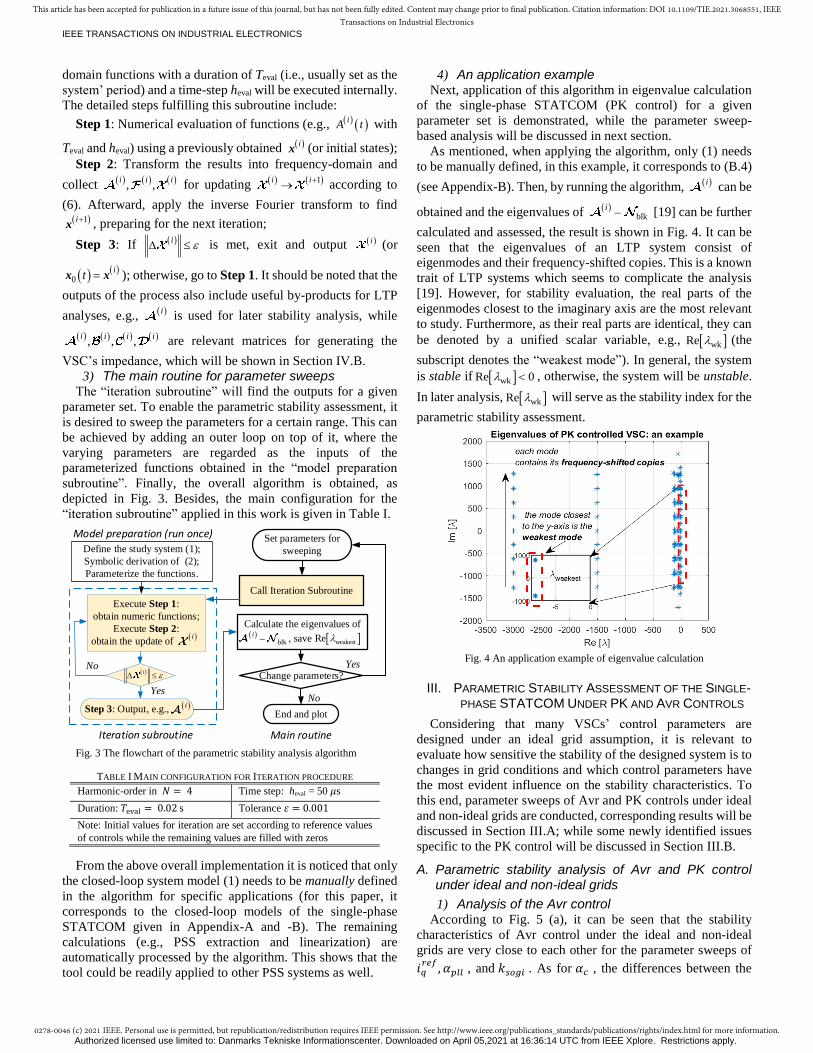
4) An application example Next, application of this algorithm in eigenvalue calculation

of the single-phase STATCOM (PK control) for a given

parameter set is demonstrated, while the parameter sweep-

based analysis will be discussed in next section.

As mentioned, when applying the algorithm, only (1) needs

to be manually defined, in this example, it corresponds to (B.4)

(see Appendix-B). Then, by running the algorithm, i can be

obtained and the eigenvalues of blk

i [19] can be further

calculated and assessed, the result is shown in Fig. 4. It can be

seen that the eigenvalues of an LTP system consist of

eigenmodes and their frequency-shifted copies. This is a known

trait of LTP systems which seems to complicate the analysis

[19]. However, for stability evaluation, the real parts of the

eigenmodes closest to the imaginary axis are the most relevant

to study. Furthermore, as their real parts are identical, they can

be denoted by a unified scalar variable, e.g., wkRe (the

subscript denotes the “weakest mode”). In general, the system

is stable if wkRe 0 , otherwise, the system will be unstable.

In later analysis, wkRe will serve as the stability index for the

parametric stability assessment.

Fig. 4 An application example of eigenvalue calculation

III. PARAMETRIC STABILITY ASSESSMENT OF THE SINGLE-PHASE STATCOM UNDER PK AND AVR CONTROLS

Considering that many VSCs’ control parameters are

designed under an ideal grid assumption, it is relevant to

evaluate how sensitive the stability of the designed system is to

changes in grid conditions and which control parameters have

the most evident influence on the stability characteristics. To

this end, parameter sweeps of Avr and PK controls under ideal

and non-ideal grids are conducted, corresponding results will be

discussed in Section III.A; while some newly identified issues

specific to the PK control will be discussed in Section III.B.

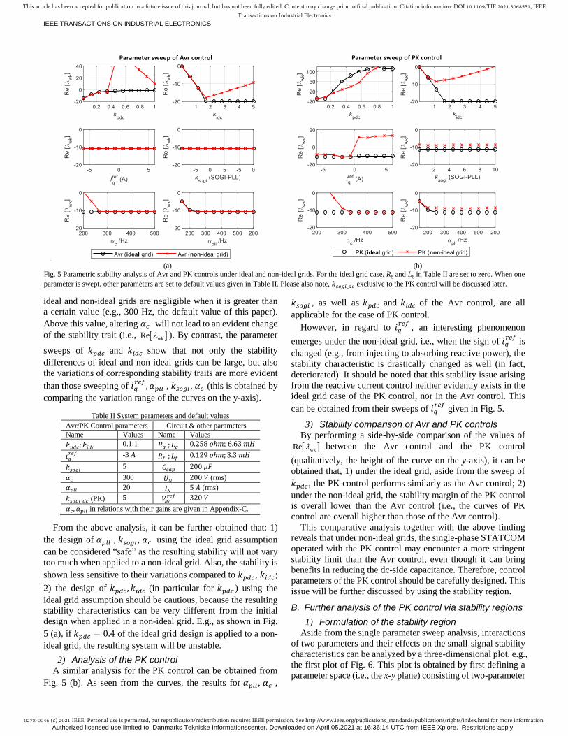
A. Parametric stability analysis of Avr and PK control under ideal and non-ideal grids

1) Analysis of the Avr control According to Fig. 5 (a), it can be seen that the stability

characteristics of Avr control under the ideal and non-ideal

grids are very close to each other for the parameter sweeps of


, 𝛼𝑝𝑙𝑙 , and 𝑘𝑠𝑜𝑔𝑖 . As for 𝛼𝑐 , the differences between the

TABLE I MAIN CONFIGURATION FOR ITERATION PROCEDURE

Harmonic-order in 𝑁 = 4 Time step: heval = 50 𝜇s

Duration: 𝑇eval = 0.02 s Tolerance 𝜀 = 0.001

Note: Initial values for iteration are set according to reference values

of controls while the remaining values are filled with zeros





ideal and non-ideal grids are negligible when it is greater than

a certain value (e.g., 300 Hz, the default value of this paper).

Above this value, altering 𝛼𝑐 will not lead to an evident change

of the stability trait (i.e., wkRe ). By contrast, the parameter

sweeps of 𝑘𝑝𝑑𝑐 and 𝑘𝑖𝑑𝑐 show that not only the stability

differences of ideal and non-ideal grids can be large, but also

the variations of corresponding stability traits are more evident

than those sweeping of 𝑖𝑞𝑟𝑒𝑓

, 𝛼𝑝𝑙𝑙 , 𝑘𝑠𝑜𝑔𝑖 , 𝛼𝑐 (this is obtained by

comparing the variation range of the curves on the y-axis).

From the above analysis, it can be further obtained that: 1)

the design of 𝛼𝑝𝑙𝑙 , 𝑘𝑠𝑜𝑔𝑖 , 𝛼𝑐 using the ideal grid assumption

can be considered “safe” as the resulting stability will not vary

too much when applied to a non-ideal grid. Also, the stability is

shown less sensitive to their variations compared to 𝑘𝑝𝑑𝑐, 𝑘𝑖𝑑𝑐;

2) the design of 𝑘𝑝𝑑𝑐, 𝑘𝑖𝑑𝑐 (in particular for 𝑘𝑝𝑑𝑐 ) using the

ideal grid assumption should be cautious, because the resulting

stability characteristics can be very different from the initial

design when applied in a non-ideal grid. E.g., as shown in Fig.

5 (a), if 𝑘𝑝𝑑𝑐 = 0.4 of the ideal grid design is applied to a non-

ideal grid, the resulting system will be unstable.

2) Analysis of the PK control A similar analysis for the PK control can be obtained from

Fig. 5 (b). As seen from the curves, the results for 𝛼𝑝𝑙𝑙 , 𝛼𝑐 ,

𝑘𝑠𝑜𝑔𝑖 , as well as 𝑘𝑝𝑑𝑐 and 𝑘𝑖𝑑𝑐 of the Avr control, are all

applicable for the case of PK control.

However, in regard to 𝑖𝑞𝑟𝑒𝑓

, an interesting phenomenon

emerges under the non-ideal grid, i.e., when the sign of 𝑖𝑞𝑟𝑒𝑓

is

changed (e.g., from injecting to absorbing reactive power), the

stability characteristic is drastically changed as well (in fact,

deteriorated). It should be noted that this stability issue arising

from the reactive current control neither evidently exists in the

ideal grid case of the PK control, nor in the Avr control. This

can be obtained from their sweeps of 𝑖𝑞𝑟𝑒𝑓

given in Fig. 5.

3) Stability comparison of Avr and PK controls By performing a side-by-side comparison of the values of

wkRe between the Avr control and the PK control

(qualitatively, the height of the curve on the y-axis), it can be

obtained that, 1) under the ideal grid, aside from the sweep of

𝑘𝑝𝑑𝑐, the PK control performs similarly as the Avr control; 2)

under the non-ideal grid, the stability margin of the PK control

is overall lower than the Avr control (i.e., the curves of PK

control are overall higher than those of the Avr control).

This comparative analysis together with the above finding

reveals that under non-ideal grids, the single-phase STATCOM

operated with the PK control may encounter a more stringent

stability limit than the Avr control, even though it can bring

benefits in reducing the dc-side capacitance. Therefore, control

parameters of the PK control should be carefully designed. This

issue will be further discussed by using the stability region.

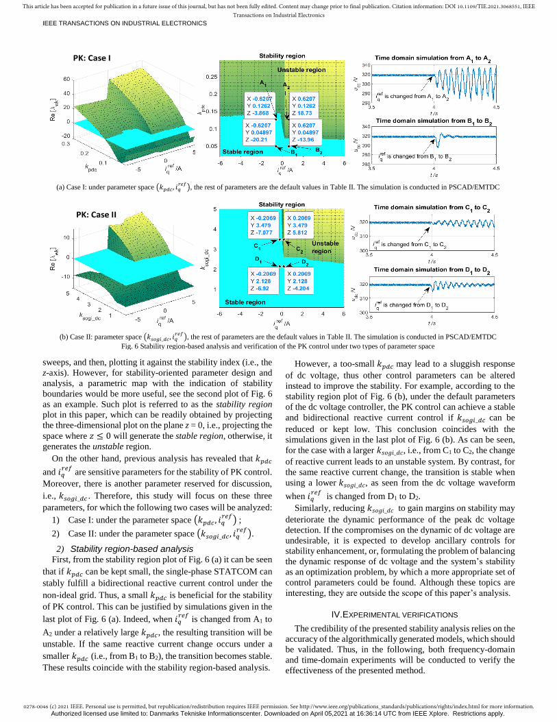
B. Further analysis of the PK control via stability regions

1) Formulation of the stability region Aside from the single parameter sweep analysis, interactions

of two parameters and their effects on the small-signal stability

characteristics can be analyzed by a three-dimensional plot, e.g.,

the first plot of Fig. 6. This plot is obtained by first defining a

parameter space (i.e., the x-y plane) consisting of two-parameter

(a) (b)

Fig. 5 Parametric stability analysis of Avr and PK controls under ideal and non-ideal grids. For the ideal grid case, Rg and Lg in Table II are set to zero. When one

parameter is swept, other parameters are set to default values given in Table II. Please also note, 𝑘𝑠𝑜𝑔𝑖_𝑑𝑐 exclusive to the PK control will be discussed later.

Table II System parameters and default values

Avr/PK Control parameters Circuit & other parameters

Name Values Name Values

𝑘𝑝𝑑𝑐; 𝑘𝑖𝑑𝑐 0.1;1 𝑅𝑔 ; 𝐿𝑔 0.258 𝑜ℎ𝑚; 6.63 𝑚𝐻


-3 A 𝑅𝑓 ; 𝐿𝑓 0.129 𝑜ℎ𝑚; 3.3 𝑚𝐻

𝑘𝑠𝑜𝑔𝑖 5 𝐶𝑐𝑎𝑝 200 𝜇𝐹

𝛼𝑐 300 𝑈𝑁 200 𝑉 (rms)

𝛼𝑝𝑙𝑙 20 𝐼𝑁 5 𝐴 (rms)

𝑘𝑠𝑜𝑔𝑖_𝑑𝑐 (PK) 5 𝑉𝑑𝑐𝑟𝑒𝑓

320 𝑉

𝛼𝑐, 𝛼𝑝𝑙𝑙 in relations with their gains are given in Appendix-C.





sweeps, and then, plotting it against the stability index (i.e., the

z-axis). However, for stability-oriented parameter design and

analysis, a parametric map with the indication of stability

boundaries would be more useful, see the second plot of Fig. 6

as an example. Such plot is referred to as the stability region

plot in this paper, which can be readily obtained by projecting

the three-dimensional plot on the plane z = 0, i.e., projecting the

space where 𝑧 ≤ 0 will generate the stable region, otherwise, it

generates the unstable region.

On the other hand, previous analysis has revealed that 𝑘𝑝𝑑𝑐

and 𝑖𝑞𝑟𝑒𝑓

are sensitive parameters for the stability of PK control.

Moreover, there is another parameter reserved for discussion,

i.e., 𝑘𝑠𝑜𝑔𝑖_𝑑𝑐 . Therefore, this study will focus on these three

parameters, for which the following two cases will be analyzed:

1) Case I: under the parameter space (𝑘𝑝𝑑𝑐 , 𝑖𝑞𝑟𝑒𝑓

) ;

2) Case II: under the parameter space (𝑘𝑠𝑜𝑔𝑖_𝑑𝑐 , 𝑖𝑞𝑟𝑒𝑓

).

2) Stability region-based analysis First, from the stability region plot of Fig. 6 (a) it can be seen

that if 𝑘𝑝𝑑𝑐 can be kept small, the single-phase STATCOM can

stably fulfill a bidirectional reactive current control under the

non-ideal grid. Thus, a small 𝑘𝑝𝑑𝑐 is beneficial for the stability

of PK control. This can be justified by simulations given in the

last plot of Fig. 6 (a). Indeed, when 𝑖𝑞𝑟𝑒𝑓

is changed from A1 to

A2 under a relatively large 𝑘𝑝𝑑𝑐, the resulting transition will be

unstable. If the same reactive current change occurs under a

smaller 𝑘𝑝𝑑𝑐 (i.e., from B1 to B2), the transition becomes stable.

These results coincide with the stability region-based analysis.

However, a too-small 𝑘𝑝𝑑𝑐 may lead to a sluggish response

of dc voltage, thus other control parameters can be altered

instead to improve the stability. For example, according to the

stability region plot of Fig. 6 (b), under the default parameters

of the dc voltage controller, the PK control can achieve a stable

and bidirectional reactive current control if 𝑘𝑠𝑜𝑔𝑖_𝑑𝑐 can be

reduced or kept low. This conclusion coincides with the

simulations given in the last plot of Fig. 6 (b). As can be seen,

for the case with a larger 𝑘𝑠𝑜𝑔𝑖_𝑑𝑐, i.e., from C1 to C2, the change

of reactive current leads to an unstable system. By contrast, for

the same reactive current change, the transition is stable when

using a lower 𝑘𝑠𝑜𝑔𝑖_𝑑𝑐, as seen from the dc voltage waveform

when 𝑖𝑞𝑟𝑒𝑓

is changed from D1 to D2.

Similarly, reducing 𝑘𝑠𝑜𝑔𝑖_𝑑𝑐 to gain margins on stability may

deteriorate the dynamic performance of the peak dc voltage

detection. If the compromises on the dynamic of dc voltage are

undesirable, it is expected to develop ancillary controls for

stability enhancement, or, formulating the problem of balancing

the dynamic response of dc voltage and the system’s stability

as an optimization problem, by which a more appropriate set of

control parameters could be found. Although these topics are

interesting, they are outside the scope of this paper’s analysis.

IV.EXPERIMENTAL VERIFICATIONS

The credibility of the presented stability analysis relies on the

accuracy of the algorithmically generated models, which should

be validated. Thus, in the following, both frequency-domain

and time-domain experiments will be conducted to verify the

effectiveness of the presented method.

PK: Case I

(a) Case I: under parameter space (𝑘𝑝𝑑𝑐, 𝑖𝑞

𝑟𝑒𝑓), the rest of parameters are the default values in Table II. The simulation is conducted in PSCAD/EMTDC

PK: Case II

(b) Case II: parameter space (𝑘𝑠𝑜𝑔𝑖_𝑑𝑐 , 𝑖𝑞

𝑟𝑒𝑓), the rest of parameters are the default values in Table II. The simulation is conducted in PSCAD/EMTDC

Fig. 6 Stability region-based analysis and verification of the PK control under two types of parameter space





A. Experimental setup

Controller (DSP+FPGA)

Main circuit

Poc

𝑖(𝑡) 𝑢(𝑡)

𝑍𝑓 𝑍𝑔

Signal generator

Superposition

Data acquisition

Single-tone injection method

𝑡

1st tone

𝑇

Nth tone

𝑇

𝑓1 𝑓𝑁

Grid voltageOsilloscope

Single-phase VSC Signal generation

Power amplifier

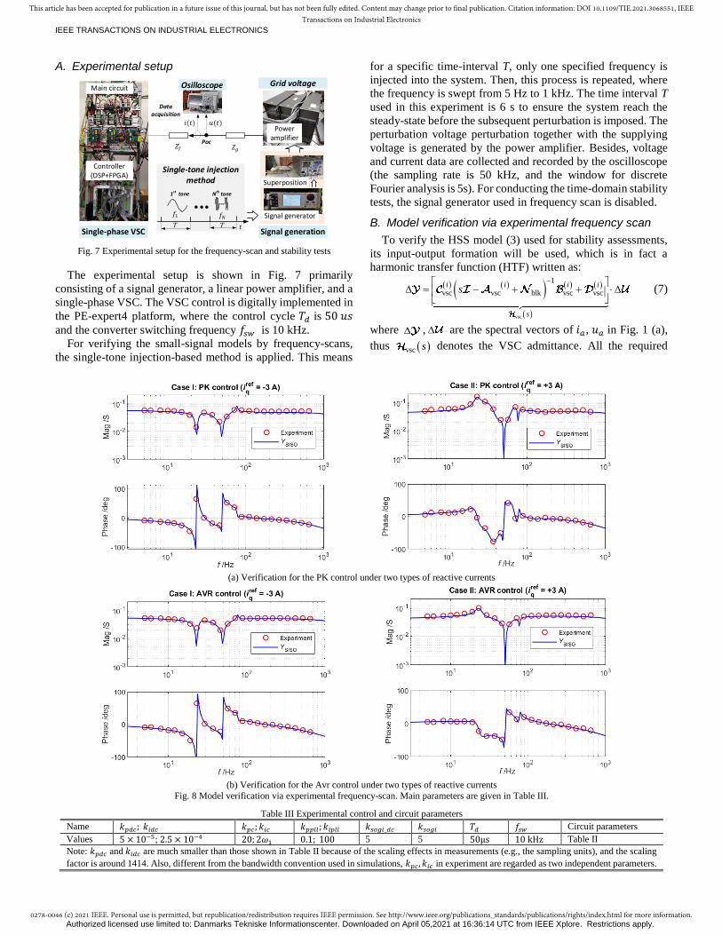
Fig. 7 Experimental setup for the frequency-scan and stability tests

The experimental setup is shown in Fig. 7 primarily

consisting of a signal generator, a linear power amplifier, and a

single-phase VSC. The VSC control is digitally implemented in

the PE-expert4 platform, where the control cycle 𝑇𝑑 is 50 𝑢𝑠

and the converter switching frequency 𝑓𝑠𝑤 is 10 kHz.

For verifying the small-signal models by frequency-scans,

the single-tone injection-based method is applied. This means

for a specific time-interval T, only one specified frequency is

injected into the system. Then, this process is repeated, where

the frequency is swept from 5 Hz to 1 kHz. The time interval T

used in this experiment is 6 s to ensure the system reach the

steady-state before the subsequent perturbation is imposed. The

perturbation voltage perturbation together with the supplying

voltage is generated by the power amplifier. Besides, voltage

and current data are collected and recorded by the oscilloscope

(the sampling rate is 50 kHz, and the window for discrete

Fourier analysis is 5s). For conducting the time-domain stability

tests, the signal generator used in frequency scan is disabled.

B. Model verification via experimental frequency scan

To verify the HSS model (3) used for stability assessments,

its input-output formation will be used, which is in fact a

harmonic transfer function (HTF) written as:

vsc

1

vsc vsc blk vsc vsci i i i

s

s

(7)

where , are the spectral vectors of 𝑖𝑎, 𝑢𝑎 in Fig. 1 (a),

thus vsc s denotes the VSC admittance. All the required

(a) Verification for the PK control under two types of reactive currents

(b) Verification for the Avr control under two types of reactive currents

Fig. 8 Model verification via experimental frequency-scan. Main parameters are given in Table III.

Table III Experimental control and circuit parameters

Name 𝑘𝑝𝑑𝑐; 𝑘𝑖𝑑𝑐 𝑘𝑝𝑐; 𝑘𝑖𝑐 𝑘𝑝𝑝𝑙𝑙; 𝑘𝑖𝑝𝑙𝑙 𝑘𝑠𝑜𝑔𝑖_𝑑𝑐 𝑘𝑠𝑜𝑔𝑖 𝑇𝑑 𝑓𝑠𝑤 Circuit parameters

Values 5 × 10−5; 2.5 × 10−4 20; 2𝜔1 0.1; 100 5 5 50μs 10 kHz Table II

Note: 𝑘𝑝𝑑𝑐 and 𝑘𝑖𝑑𝑐 are much smaller than those shown in Table II because of the scaling effects in measurements (e.g., the sampling units), and the scaling

factor is around 1414. Also, different from the bandwidth convention used in simulations, 𝑘𝑝𝑐, 𝑘𝑖𝑐 in experiment are regarded as two independent parameters.





matrices can be obtained from the iteration subroutine in Fig. 3.

As vsc s is a multi-input and multi-output (MIMO) system,

its direct verification via the frequency scan is cumbersome,

where a large number of perturbations is required, e.g., for a

2 1N dimensional HTF, 2 1N times of injections are needed

for measuring the frequency response of the HTF at each

frequency point [19]. To allow a simpler verification, vsc s

can be first converted into a single-input and single-output

(SISO) equivalent model SISOY s according to [28]. Then,

SISOY s can be verified instead of vsc s so that the typical

frequency scan routine as illustrated above can be applied.

Based on this method, the frequency responses of SISOY s

under Avr and PK controls will be compared with experiments,

where the following two cases are tested: 1) Case I: Inject

reactive power by controlling a negative reactive current, i.e.,


< 0; 2) Case II: Absorb reactive power by controlling a

positive reactive current, i.e., 𝑖𝑞𝑟𝑒𝑓

> 0.

According to the comparative results given in Fig. 8 (a), it

can be seen that the frequency responses of PK control under

both of the cases are consistent with experiments, and the same

conclusion applies to Avr control, as indicated by the results in

Fig. 8 (b). Overall, this experimental frequency scan indicates

that the generated models using the presented method are valid,

which in turn justifies the validity of the harmonic-order N used

in the iteration model (as is introduced in Section II.C).

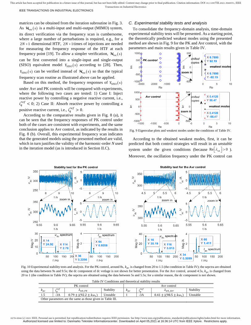
C. Experimental stability tests and analysis

To consolidate the frequency-domain analysis, time-domain

experimental stability tests will be presented. As a starting point,

the theoretically predicted weakest modes using the presented

method are shown in Fig. 9 for the PK and Avr control, with the

parameters and main results given in Table IV.

Fig. 9 Eigenvalue plots and weakest modes under the conditions of Table IV.

According to the obtained weakest modes, first, it can be

predicted that both control strategies will result in an unstable

system under the given conditions (because wkRe 0 ).

Moreover, the oscillation frequency under the PK control can

Fig. 10 Experimental stability tests and analysis. For the PK control, around 8s, 𝑘𝑝𝑐 is changed from 20 to 1.5 (the condition in Table IV); the sepctra are obtained

using the data between 9s and 9.5s; the dc component of dc votlage is not shown for better presentation. For the Avr control, around 4.5s, 𝑘𝑝𝑐 is changed from

20 to 1 (the condition in Table IV); the sepctra are obtained using the data between 5s and 5.5s; for a similar reason, the dc component is not shown.

Table IV Conditions and theoretical stability results

PK control Avr control

𝑘𝑝𝑐 𝑖𝑞𝑟𝑒𝑓

𝜆𝑤𝑘_𝑃𝐾 Stability 𝑘𝑝𝑐 𝑖𝑞𝑟𝑒𝑓

𝜆𝑤𝑘_𝐴𝑣𝑟 Stability

1.5 -3A 0.79 ± j(92.2 ± 𝑘𝜔1) Unstable 1 -3A 0.41 ± j(98.5 ± 𝑘𝜔1) Unstable

Other parameters are the same as those given in Table III.





be estimated by: osc_PK 14.67 50f k Hz , 0,1,2,...k (i.e., from

wkIm ), while for the Avr control, it is estimated as:

osc_PK 15.67 50f k Hz .

To verify these theoretical stability results, time-domain

stability tests are conducted using the conditions as Fig. 9.

According to the experimental results in Fig. 10, it can be

clearly seen that when the control parameters of the Avr and PK

controls are set to those given in Table IVTable III, small-signal

instability in the form of oscillations occurs for both systems.

Further, by inspecting the spectra of dc voltage and ac current

of the PK control, it can be obtained that the oscillation modes

are frequency shifted copies of 14 Hz, which is very close to the

theoretical result, i.e., frequency shifted copies of 14.67 Hz. On

the other hand, the oscillation modes of the Avr control from

experiments are shown to consist of frequency-shifted copies of

16 Hz, which is also very close to its predictions, i.e.,

frequency-shifted copies of 15.67 Hz.

Therefore, the experimental stability tests further confirm the

validity and accuracy of the presented method, thus ensuring

the credibility of the conclusions obtained in this paper.

V. CONCLUSIONS

This paper presents a comprehensive stability analysis and

comparison of the single-phase STATCOM using the PK and

Avr control. Apart from the known merits of PK control in

enabling reduced dc-side capacitance, this paper achieved an in-

depth understanding of the PK control in view of its parametric

stability performance. The main conclusions and findings are:

1) Under non-ideal grids, the PK control is prone to be

unstable when absorbing reactive power, as a consequence of

high sensitivity to some of its control parameters, e.g., 𝑘𝑠𝑜𝑔𝑖_𝑑𝑐

and 𝑘𝑝𝑑𝑐 . By contrast, the Avr control is shown to be less

susceptible to this issue and overall exhibits a better stability

performance than the PK control.

2) Control parameter design of PK control using ideal grid

assumption should be of great caution, particularly for those

parameters identified to be sensitive to grid condition changes,

e.g., 𝑘𝑠𝑜𝑔𝑖_𝑑𝑐 and 𝑘𝑝𝑑𝑐. Otherwise, the designed system cannot

be ensured to be stable when connected to non-ideal grids.

3) Alleviating the potential stability risks of the PK control

can be achieved by properly designing the control parameters,

which can be assisted by the presented stability plot.

Besides, according to the various analyses presented in this

paper, it also demonstrates that the developed tool has a great

potential of being promoted to other PSS-based converter

systems for fast and efficient parametric stability tests.

APPENDIX

A. State-space model under Avr control

State-space modeling of the grid-VSC system can be fulfilled

by first listing all the state equations of controllers and circuit

elements; then connecting them via control diagrams and basic

circuit laws. Since this process is straightforward (which can be

readily obtained from Fig. 1 (a) and (b)), only the final results

along with necessary explanations will be given in the next.

1) SOGI-QSG for synchronization

sogia 1 sogi 1 b

sogi_synsogib

ˆ ˆ

ˆ

a a

a

x k u u u

x u

f (A.1)

where the in-phase and quadrature outputs of the SOGI-QSG

are sogiaˆau x and b 1 sogibu x .

2) SRF-PLL

ppll pllpll

PLLipll qpll

qk u x

k ux

f (A.2)

where q pll 1 a pll 1 bˆ ˆsin cosu t u t u . In which, the

substitution pll pll 1t is used.

3) dc voltage and controller

2 2dc idc dc dc_ref dc_Avrx k u V f (A.3)

where the output is ref 2 2d pdc dc dc_ref dci k u V x .

4) PR-based current control

refpra 1 a a 1 prb

PRprb pra

x i i x

x x

f (A.4)

where ref ref refa d 1 pll q 1 pllcos sini i t i t , and the

current PR controller output is:

ref ref ica pc a a pra

dc 1

21 km k i i x

u

(A.5)

where 𝑚𝑎𝑟𝑒𝑓

is the modulation signal as shown in Fig. 1 (a).

5) Circuit model

The circuit model shown below includes the dc capacitor,

ac/dc modulation, converter filter as well as the grid impedance.

refrefa dc g f g adc a a

circap fa

,

T

g

m u u R R iu m i

C L Li

f (A.6)

In which, the PoC voltage used in (A.1) can be obtained as:

refa f g f g g f a g a dcu k u k R k R i k m u (A.7)

where f f f/ gk L L L , g f1k k .

Combing (A.1)-(A.7) will result in the final closed-loop

model of the Avr control in a similar formation of (1):

cl_Avr

cl_Avr

, ,

, ,

t

t

x f x u

y g x u (A.8)

where cl_Avr g Cx , 2 refdc_ref q g[ , , ]V i uu , and 1 4 1 4[ ,1, ] C 0 0

dc pra prb dc a sogia sogib pll pll, , , , , , , ,T

x x x u i x x x

x ,

cl_Avr dc_Avr PR cir sogi_syn PLL, , , ,T

f f f f f f .

B. State-space model under PK control

The modeling of PK control is similar to that of Avr control.

One major difference is the adoption of the SOGI-based filter

(see Fig. 2 (a)) for peak-value dc voltage estimation (i.e., 2dc_pku ).

The applied SOGI-QSG in the filter has the same structure as

(A.1), which can be written as:





2 2 22 sogi_dc dc dc_α 2 dc_βsogia_dc

sogi_dc2

sogib_dcdc_α

k u u ux

x u

f (B.1)

where 2 12 , 2dc_α sogia_dcu x , 2

dc_β 2 sogib_dcu x . The output

of the filter (i.e., 2dc_pku ) can be represented as:

2 2 2 2dc_pk pk dc dc_α dc_β sogi_dc, , ,u g u u u k (B.2)

where function pkg denotes the result of algebraic

operations performed on the inputs (according to Fig. 2 (a)).

Given this output, (A.3) is modified as:

2 2dc idc dc_pk dc_ref dc_PKx k u V f (B.3)

Combining (B.1)-(B.3), (A.2), and (A.4)-(A.7) results in the

final closed-loop model of PK control similar to (1):

cl_PK

cl_PK

, ,

, ,

t

t

x f x u

y g x u (B.4)

where cl_PK g Cx , 2 refdc_ref q g[ , , ]V i uu , and 1 6 1 4[ ,1, ] C 0 0 .

sogia_dc sogib_dc dc pra prb dc a sogia sogib pll pll, , , , , , , , , ,T

x x x x x u i x x x

x , ,

cl_PK sogi_dc dc_PK PR cir sogi_syn PLL, , , , ,T

f f f f f f f .

In this paper, (A.8) and (B.4) correspond to the generic

system (1), i.e., the input of “model preparation subroutine”.

C. Definition of current control and PLL bandwidths

In this paper, the relations between the defined closed-loop

bandwidths and their controller gains are: 2

pc c f ic c f2 , 2k L k L ,

2

ppll pll ipll pll2 / , 2 /N Nk U k U .

REFERENCES

[1] H. Liu, X. Xie, J. He, J, T. Xu, Z. Yu, C. Wang, C. Zhang, "Subsynchronous Interaction Between Direct-Drive PMSG Based Wind Farms and Weak AC Networks," in IEEE Transactions on Power Systems, vol. 32, no. 6, pp. 4708-4720, Nov. 2017.

[2] C. Li, “Unstable Operation of Photovoltaic Inverter from Field Experiences,” in IEEE Transactions on Power Delivery, Vol. 33, No. 2, April 2018, pp. 1013-1015

[3] M. Belkhayat, “Stability criteria for AC power systems with regulated loads,” Ph.D. dissertation, Purdue University, USA, 1997.

[4] J. Sun, "Impedance-Based Stability Criterion for Grid-Connected Inverters," in IEEE Transactions on Power Electronics, Vol. 26, No. 11, November 2011, pp. 3075-3078

[5] X. Wang and F. Blaabjerg, "Harmonic Stability in Power Electronic Based Power Systems: Concept, Modeling, and Analysis," in IEEE Transactions on Smart Grid, Vol. 10, No. 3, May 2019, pp. 2858-2870

[6] D. Dong, B. Wen, D. Boroyevich, P. Mattavelli and Y. Xue, "Analysis of Phase-Locked Loop Low-Frequency Stability in Three-Phase Grid-Connected Power Converters Considering Impedance Interactions," in IEEE Transactions on Industrial Electronics, vol. 62, no. 1, pp. 310-321, Jan. 2015.

[7] B. Wen, D. Boroyevich, R. Burgos, P. Mattavelli and Z. Shen, "Small-Signal Stability Analysis of Three-Phase AC Systems in the Presence of Constant Power Loads Based on Measured d-q Frame Impedances," in IEEE Transactions on Power Electronics, Vol. 30, No. 10, October 2015, pp. 5952-5963,.

[8] M. Cespedes and J. Sun, "Impedance Modeling and Analysis of Grid-Connected Voltage-Source Converters," in IEEE Transactions on Power Electronics, Vol. 29, No. 3, pp. March 2014, 1254-1261

[9] X. Wang, L. Harnefors and F. Blaabjerg, "Unified Impedance Model of Grid-Connected Voltage-Source Converters," in IEEE Transactions on Power Electronics, Vol. 33, No. 2, February 2018, pp. 1775-1787

[10] A. Rygg, M. Molinas, C. Zhang and X. Cai, "A Modified Sequence-Domain Impedance Definition and Its Equivalence to the dq-Domain Impedance Definition for the Stability Analysis of AC Power Electronic Systems," in IEEE Journal of Emerging and Selected Topics in Power Electronics, vol. 4, no. 4, Dec. 2016, pp. 1383-1396

[11] L. Harnefors, M. Bongiorno and S. Lundberg, "Input-Admittance Calculation and Shaping for Controlled Voltage-Source Converters," in IEEE Transactions on Industrial Electronics, vol. 54, no. 6, December 2007, pp. 3323-3334

[12] L. Harnefors, “Modeling of Three-Phase Dynamic Systems Using Complex Transfer Functions and Transfer Matrices,” in IEEE Trans. Ind. Electron, vol. 54, no. 4, pp. 2239–2248, 2007.

[13] Z. W Yao, P. G. Therond, and B. Davat, "Frequency Characteristic of AC Power System", IFAC 12th Triennial World Congress, Sydney, Australia, 1993, pp. 737-740.

[14] N. M. Wereley, Analysis and control of linear periodically time varying systems, Diss. Massachusetts Institute of Technology, 1990.

[15] P. Vanassche, G. Gielen and W. M. Sansen, "Systematic modeling and analysis of telecom frontends and their building blocks," Springer Science & Business Media, 2006.

[16] E. Mollerstedt and B. Bernhardsson, "Out of control because of harmonics-an analysis of the harmonic response of an inverter locomotive," in IEEE Control Systems Magazine, vol. 20, no. 4, pp. 70-81, Aug. 2000.

[17] Ö. C. Sakinci and J. Beerten, "Generalized Dynamic Phasor Modeling of the MMC for Small-Signal Stability Analysis," in IEEE Transactions on Power Delivery, vol. 34, no. 3, pp. 991-1000, June 2019.

[18] C. Guo, J. Yang and C. Zhao, "Investigation of Small-Signal Dynamics of Modular Multilevel Converter Under Unbalanced Grid Conditions," in IEEE Transactions on Industrial Electronics, vol. 66, no. 3, pp. 2269-2279, March 2019.

[19] V. Salis, A. Costabeber, S. M. Cox and P. Zanchetta, "Stability Assessment of Power-Converter-Based AC systems by LTP Theory: Eigenvalue Analysis and Harmonic Impedance Estimation," in IEEE Journal of Emerging and Selected Topics in Power Electronics, vol. 5, no. 4, December 2017, pp. 1513-1525

[20] Y. Liao, Z. Liu, H. Zhang and B. Wen, "Low-Frequency Stability Analysis of Single-Phase System With dq-Frame Impedance Approach—Part I: Impedance Modeling and Verification," in IEEE Transactions on Industry Applications, Vol. 54, No. 5, October 2018, pp. 4999-5011.

[21] H. Wang, W. Mingli and J. Sun, "Analysis of Low-Frequency Oscillation in Electric Railways Based on Small-Signal Modeling of Vehicle-Grid System in dq Frame," in IEEE Transactions on Power Electronics, vol. 30, no. 9, pp. 5318-5330, Sept. 2015.

[22] H. Zhang, Z. Liu and S. Wu, "Sequence Impedance Modeling and Stability Analysis of Single-Phase Converters," 2018 21st International Conference on Electrical Machines and Systems, ICEMS 2018, Jeju, Korea, pp. 2234-2239.

[23] S. Shah and L. Parsa, "On impedance modeling of single-phase voltage source converters," 2016 IEEE Energy Conversion Congress and Exposition¸ ECCE 2016, Milwaukee, WI, 2016, pp. 1-8.

[24] J. Carter, C. J. Goodman and H. Zelaya, "Analysis of the single-phase four-quadrant PWM converter resulting in steady-state and small-signal dynamic models", IEE Proc. Elect. Power Appl., vol. 144, no. 4, pp. 241-247, Jul. 1997.

[25] T. Isobe, D. Shiojima, K. Kato, Y. R. R. Hernandez and R. Shimada, "Full-Bridge Reactive Power Compensator With Minimized-Equipped Capacitor and Its Application to Static Var Compensator," in IEEE Transactions on Power Electronics, vol. 31, no. 1, pp. 224-234, Jan. 2016.

[26] T. Isobe, L. Zhang, H. Tadano, J. A. Suul and M. Molinas, "Control of DC-capacitor peak voltage in reduced capacitance single-phase STATCOM," IEEE 17th Workshop on Control and Modeling for Power Electronics, COMPEL 2016, Trondheim, pp. 1-8.

[27] Y. Sun, Y. Liu, M. Su, W. Xiong, J. Yang, “Review of Active Power Decoupling Topologies in Single-Phase Systems,” in IEEE Transactions on Power Electronics, vol. 31, no. 7, July 2016, pp. 4778–4794.

[28] C. Zhang, M. Molinas, S. Føyen, J. A. Suul and T. Isobe, "An Integrated Method for Generating VSCs’ Periodical Steady-State Conditions and

HSS-Based Impedance Model," in IEEE Transactions on Power Delivery,

vol. 35, no. 5, pp. 2544-2547, Oct. 2020.





Chen Zhang received the B.Eng. degree from the China University of Mining and Technology, China,

and the Ph.D. from Shanghai Jiao Tong University,

China, in 2011 and 2018 respectively. He was a

Postdoctoral Research Fellow at the Department of

Engineering Cybernetics of NTNU, from March 2018

to October 2020. Currently, he is a postdoc with the Department of Electrical Engineering, Technical

University of Denmark, Lyngby, Denmark. His

research interest is modeling and stability analysis of VSC-based energy conversion systems, where the aim is to reveal the fundamental dynamics and

stability mechanisms of renewable energies with VSCs as the grid interface.

Takanori Isobe (M'07) was born in Hamamatsu, Japan, in 1978. He received the B.Eng. degree in

physical electronics, the M.Eng. degree in nuclear

engineering, and the D.Eng. degree in energy sciences from the Tokyo Institute of Technology, Tokyo, Japan,

in 2003, 2005, and 2008, respectively. From 2008 to

2010 and from 2012 to 2013, he was a Researcher with the Tokyo Institute of Technology, where from 2010

to 2012, he was an Assistant Professor. From 2013 to

2014, he was with MERSTech, Tokyo. In 2013, he joined the University of Tsukuba, Tsukuba, Ibaraki, Japan, where he is currently

an Associate Professor at the Faculty of Pure and Applied Sciences. His

research interests include static reactive power compensators and soft-switching power converters. Dr. Isobe is a Member of the Institute of Electrical

Engineers of Japan and the Japan Institute of Power Electronics.

Jon Are Suul (M'11) received the M.Sc. degree in

energy and environmental engineering and the Ph.D.

degree in electric power engineering from the Norwegian University of Science and Technology

(NTNU), Trondheim, Norway, in 2006 and 2012,

respectively. From 2006 to 2007, he was with SINTEF Energy Research, Trondheim, where he was working

with simulation of power electronic converters and

marine propulsion systems until starting his Ph.D. studies. He returned to SINTEF Energy Research as a

Research Scientist in 2012, first in a part-time position while working as a part-

time Postdoctoral Researcher with the Department of Electric Power

Engineering of NTNU until 2016. Since August 2017, he has been an Adjunct

Associate Professor with the Department of Engineering Cybernetics, NTNU.

His research interests are mainly related to modeling, analysis, and control of power electronic converters in power systems, renewable energy applications,

and electrification of transport. He is Associate Editor in the IEEE Journal of

Emerging and Selected Topics in Power Electronics and in the IEEE Journal of Emerging and Selected Topics in Industrial Electronics

Tomislav Dragičević (S’09-M’13-SM’17) received

the M.Sc. and the industrial Ph.D. degrees in Electrical Engineering from the Faculty of Electrical

Engineering, University of Zagreb, Croatia, in 2009

and 2013, respectively. From 2013 until 2016 he has been a Postdoctoral researcher at Aalborg University,

Denmark. From 2016 until 2020 he was an Associate

Professor at Aalborg University, Denmark. Currently, he is a Professor at the Technical

University of Denmark. He made a guest professor stay at Nottingham

University, UK during spring/summer of 2018. His research interest is application of advanced control, optimization and artificial intelligence inspired

techniques to provide innovative and effective solutions to emerging challenges

in design, control and diagnostics of power electronics intensive electrical distributions systems and microgrids. He has authored and co-authored more

than 300 technical publications (more than 150 of them are published in

international journals, mostly in IEEE), 10 book chapters and a book in the field. He serves as an Associate Editor in the IEEE TRANSACTIONS ON

INDUSTRIAL ELECTRONICS, in IEEE TRANSACTIONS ON POWER

ELECTRONICS, in IEEE Emerging and Selected Topics in Power Electronics and in IEEE Industrial Electronics Magazine. Dr. Dragičević is a recipient of

the Končar prize for the best industrial PhD thesis in Croatia, a Robert Mayer

Energy Conservation award, and he is a winner of an Alexander von Humboldt fellowship for experienced researchers.

Marta Molinas (M'94) received the Diploma degree in electromechanical engineering from the National

University of Asuncion, Asuncion, Paraguay, in

1992; the Master of Engineering degree from Ryukyu

University, Japan, in 1997; and the Doctor of

Engineering degree from the Tokyo Institute of

Technology, Tokyo, Japan, in 2000. She was a Guest Researcher with the University of Padova, Padova,

Italy, during 1998. From 2004 to 2007, she was a

Postdoctoral Researcher with the Norwegian University of Science and Technology (NTNU) and from 2008-2014 she has

been professor at the Department of Electric Power Engineering at the same

university. She is currently Professor at the Department of Engineering Cybernetics, NTNU. Her research interests include stability of power

electronics systems, harmonics, instantaneous frequency, and non-stationary

signals from the human and the machine. She is Associate Editor for the IEEE Journal JESTPE, IEEE PELS Transactions and Editor of the IEEE Transactions

on Energy Conversion. Dr. Molinas has been an AdCom Member of the IEEE

Power Electronics Society from 2009 to 2011.


Parametric Stability Assessment of Single-phase Grid-tied ...

Documents

Transcript of Parametric Stability Assessment of Single-phase Grid-tied ...