Va

Fa

b

c

d

ARRA

KVTRNMB

1

trtf

irfAa1RKttm

T

an

0h

J. of Supercritical Fluids 81 (2013) 67– 78

Contents lists available at SciVerse ScienceDirect

The Journal of Supercritical Fluids

jou rn al hom epage: www.elsev ier .com/ locate /supf lu

iscosity prediction by computational method and artificial neural networkpproach: The case of six refrigerants

orouzan Ghaderia, Amir Hosein Ghaderib,d,∗, Bijan Najafia, Noushin Ghaderi c

College of Chemistry, Isfahan University of Technology, Isfahan, Iran 84154Neuroscience Lab, University of Tabriz, Tabriz, IranFaculty of Engineering, Shahrekord University, Shahrekord, IranNeuroscience Research Center, Kerman University of Medical Sciences, Kerman, Iran

a r t i c l e i n f o

rticle history:eceived 11 January 2013eceived in revised form 28 April 2013ccepted 29 April 2013

eywords:

a b s t r a c t

There are some computational models for fluids viscosity calculation. However, each of these models isreliable in confined density. In this comparative study two methods are evaluated for viscosity predictionin all range of density. We determine the effectiveness of each of the models and we demonstrate thestrengths and weaknesses of them. Viscosity of the six refrigerants is calculated by some computationalmodels based on Chapman–Enskog and Rainwater–Friend theories. Then a feed forward artificial neural

iscosityransport propertiesefrigeranteural networkultilayer perceptrons

ackpropagation

network (ANN) with multilayer perceptrons is used to viscosity prediction and finally two methods(computational models and artificial neural network) are comparing. It is concluded that there is noopinion by computational methods to calculate viscosity from low to high density. The results show thatprediction accuracy of computational models in low and moderate densities is good as ANN method.However artificial neural network has very good accuracy in high densities while computational methodis defeated when the density is more than 8.

. Introduction

Transport properties, especially for refrigerants, are vital inoday’s technology. It is necessary to have specific informationegarding the transport properties of refrigerants in order to be ableo plan chemical process reactors and to identify intermolecularorces.

The thermodynamic properties of refrigerants are consideredn many articles. A fundamental equation for dichlorodifluo-omethane (R12) is presented by Penoncello et al. that it is validor temperatures from 175 K to 600 K with pressures to 70 MPa [1].

theoretical and experimental study of equation of state of R14 isccomplished in range of temperature 95–413 K and pressure up to100 bar [2]. Also in other work the thermodynamic properties of14 are considered in temperature range from 12 K to 145.12 K [3].iselev et al. presented a practical approach for transport proper-

ies of R32. They obtained viscosity and thermal conductivity andheir finding is valid in the vapor–liquid critical region [4]. The ther-

ophysical properties of fluids including R115 are investigated in

∗ Corresponding author at: Neuroscience Lab, University of Tabriz, Tabriz, Iran.el.: +98 4113809217.

E-mail addresses: forouzanghaderi@yahoo.com (F. Ghaderi),mirhoseinghaderi@gmail.com, amirhoseinghaderi@yahoo.com (A.H. Ghaderi),ajafi@cc.iut.ac.ir (B. Najafi), ghaderi.nooshin@eng.sku.ac.ir (N. Ghaderi).

896-8446/$ – see front matter. Crown Copyright © 2013 Published by Elsevier B.V. All rittp://dx.doi.org/10.1016/j.supflu.2013.04.017

Crown Copyright © 2013 Published by Elsevier B.V. All rights reserved.

Makita study [5]. Also the viscosity coefficient of the refrigerantR152a has been measured in some studies [6].

Specific equations for the transport properties of gases werefound by Maxwell and Boltzman in the decade of 1860–1870. By1917, these equations were solved by Sydney Chapman and DavidEnskog separately [7]. These two scientists only solved the Boltz-man equation for mono atomic dilute gases. Because this theoryonly considered the collision of two molecules, the conclusionobtained was invalid for denser gases due to the fact that 3 moleculecollisions occurred. Calculation of the collision integral � wascarried out by Najafi et al. [8]. In this work, they divided the tem-perature into three sections: low, moderate, and high. Within eachsection a separate equation was found for the calculation of � foreach [8]. � is dependent on the temperature and the intermolecularpotential between two particles.

In 2000, based on Aziz potential, an equation was giventhat was applicable to all temperatures [9]. In 1980, Rainwa-ter and Friend presented a method to calculate the transportproperties of gases by calculating Bx (second transport virialcoefficient) in moderate density. Lennard–Jones potential was usedin this method [10]. Because these models did not consider theeffects that particles have upon one another, there was a devia-

tion from reality which caused the model to be incomplete. A moreprecise model was presented by Aziz et al. [11]. After that, Najafiet al. and then Behnejad and Miralinaghi presented semi-empiricalmodels for inter atomic potential to calculate the second transport

ghts reserved.

6 ercriti

vcvm

sssedco

dbmmrasp

sTvwCvp[udtldtmcdivs(wwt

sCctip(vniTbrRtdemf

8 F. Ghaderi et al. / J. of Sup

irial coefficient Bx [12–14]. Hashemi and Tafreshi calculated vis-osity in zero density based on the Chapman–Enskog method andiscosity in moderate density based on the Rainwater method forono atomic fluids [15].From 1928 to 1939 a specific relation between corresponding

tates and intermolecular forces was presented for the first timeeparately by Michels, Pitzer and Deboer. They found that it is pos-ible to expand the principle of corresponding states from the statequation to transport properties [16]. The viscosity of gases in highensity with use of corresponding states correlation functions wasalculated by Najafi et al. [12,13]. It is concluded that there is nopinion to calculate transport properties from low to high density.

Computational methods are reliable methods for viscosity pre-iction in partly wide range of density and moderate density rangeut in higher density, these methods are defeated. Therefore oneethod is required to solve this problem. Recently some nonlinearethods are proposed for such predictions [17–19]. Artificial neu-

al network (ANN) is a nonlinear method that is a very beneficialpproach for prediction and classification in very contexts such asignal processing [20–22], climate predictions [23–25], economyredictions [26,27] and so on.

In specify thermodynamic properties of refrigerants by ANNome researches are accomplished. Arcaklioglu et al. used ANN forhermodynamic analyses of refrigerant mixtures. They have usedarious ratios of seven refrigerant mixtures of HFCs and HCs alongith three CFCs (R12, R22, R502). They were used as inputs while theoefficients of performances and total irreversibility of refrigerantsalues were the outputs [28]. In this case Austin et al. used backropagation algorithm for mixed refrigerants suitability analysis29]. Also some researches are accomplished in viscosity equationsing multilayer feed forward neural network [30,31]. Thermo-ynamic properties (specific volume, enthalpy and entropy) ofwo alternative refrigerants (R508b and R407c) for both saturatediquid–vapor region (wet vapor) and superheated vapor region areetermined using ANN by Sozen et al [32,33]. Coquelet et al. usedwo approaches (a neural network model and a thermodynamic

odel implying equations of state and several mixing rules) toalculate thermodynamics properties like enthalpy, entropy fromensity values [34]. Singh et al. accomplished an article in compar-

ng the performances of the training functions for predicting thealue of specific heat of refrigerant in vapor absorption refrigerationystem. They compare performances of three training functionsTRAINBR, TRAINCGB and TRAINCGF) used for training neural net-ork and found that TRAINBR is the most suitable training functionith the experimental data of specific heat capacity among the

hree functions [35].In this paper, viscosity of the six refrigerants is calculated by

ome computational methods. In a partly wide range of densityhapman–Enskog method is used. In the proposed method theollision integral (�) is obtained by using the most accurate poten-ial functions and a correlation function dependent on ln T* isntroduced in a wide temperature range, where T* is reduced tem-erature. The Rainwater–Friend theory and viscosity in zero density�0) and second viscosity virial coefficient (B�) are used to calculateiscosity in moderate density (up to 2 mol/L). Then a feed forwardeural network is used to calculating viscosity for these refrigerants

n all ranges of density and finally two methods are comparing.he experimental data are taken from the suggested referencesy National Institute of Standards and Technology (NIST) for sixefrigerants: R12 [36–41], R14 [42–50], R32 [51–58], R115 [59–62],143 [63–65], and R152 [66,67]. The results indicate that, compu-ational methods show better accuracy in partly wide range of

ensity for some refrigerants and found authentic results. How-ver, according to the results, the ANN approach is a valuableethod in higher density when the computational methods are

ailed.

cal Fluids 81 (2013) 67– 78

This paper is organized as follows: scientific methods for com-puting viscosity are described in Section 2. Section 3 is devoted toexplanation of feedforward neural networks and back-propagationalgorithm. Application of calculation methods for prediction ofrefrigerant viscosity is statement in Section 4. Application of theANN on R12 viscosity prediction is exposited in Section 5 andSections 6 and 7 are devoted to state discussion and conclusions.

2. Scientific methods for computing viscosity over a widerange of density

2.1. Refrigerant viscosity in zero density

Viscosity in low density, �0 is obtained by the Chapman–Enskogkinetic theory and following equation [68]:

�0 = MT1/2

�2�(T∗)(1)

where M is molecular mass, � is viscosity and T* is reduced tem-perature that equals KT/�. In which K is the Boltzman constant, T isabsolute temperature and � is potential well depth and � is colli-sion integral. By using Aziz potential [11] and equations offered byNajafi et al. [8], the applicable equation to all temperature rangesfor the calculation of �T∗ (2,2) is as follow [69],

�T∗ (2,2) = exp6∑

i=0

ai(ln T∗)i (2)

where expansion coefficients are:

a0 = 4.369 × 10−1 ± 7.8 × 10−4 a1 = −4.505 × 10−1 ± 1.3 × 10−3

a2 = 5.326 × 10−2 ± 8.1 × 10−4 a3 = 3.519 × 10−2 ± 9.2 × 10−4

a4 = −1.751 × 10−2 ± 4 × 10−4 a5 = 2.772 × 10−3 ± 7 × 10−5

a6 = −1.529 × 10−4 ± 4.3 × 10−6

In the Chapman–Enskog theory it is assumed that the container’sdimensions are large in contrast to the mean free path. Thereforethis theory is not completely valid in low temperatures and highdensities.

2.2. Refrigerant viscosity in moderate density

Viscosity prediction method in moderate densities (up to2 mol/L) employs the RF theory. In 1980s, Rainwater and Friend[10,70,71] have introduced a microscopically based theoreticalmodel for the calculation of the second transport virial coefficientswhich contains the effects of two body collisional transfer, three-monomer and monomer–dimer collisions. We have used RF theorybecause of its adhesion with the corresponding states residual func-tion and this is a reliable model for computing the viscosity ofrefrigerants over a relatively wide temperature and pressure range.According to this theory, in the moderate range of density, viscos-ity, �, can be found with the following expansion when B� is thesecond virial coefficient of viscosity [10,12]:

� = �0(1 + B�� + �2�2 + · · ·) (3)

B� is reduced to B∗�:

B∗� = B�

�3(4)

B∗� is composed of three statements [70,71]:

B∗� = B(2)∗

� + B(M−D)∗� + B(3)∗

� (5)

ercriti

Bvlcolc

B

w

ue

�

2

epa

�

�ou

�

ttt

w

ipp

�

wi

3a

wf

F. Ghaderi et al. / J. of Sup

(2)∗� which is considered as collision transfer, affects the secondirial coefficient. In addition it represents the contribution of non-ocality of monomer–monomer collisions. If density increases, B(3)∗

� ,hance of triple molecular collision will increase, which then effectsn viscosity. B(M−D)∗

� is the contribution of monomer–dimer col-isions. Najafi et al. [10,12] presented the reduced second virialoefficient of viscosity based on real aziz potential:

∗� =

6∑i=0

bi(T∗)−i (6)

here

b0 = −0.2487 b1 = 2.925 b2 = 1.914 b3 = −7.749

b4 = 5.680 b5 = −2.224 b6 = 0.2123

The viscosity of fluids depends on the number of molecules pernit volume, hence, this quantity times Avogadro’s number. Thequation � = �0(1 + B��) rearranges to become:

= �0(1 + NA�3B∗��) (7)

.3. Refrigerant viscosity in high density

In high density residual viscosity is defined as ��. It is depend-nt of density and there is a regular dependence between transportroperties like viscosity with density [16]. Thus it can be writtens:

(T,�) = �(T)0 + ��(T,�) + ��c(T,�), (8)

�c(T,�) is residual viscosity and ��c shows critical viscosity. Sinceur calculations are out of critical range, ��c(T,�) is ignored. Resid-al viscosity is dependent upon temperature and density [12,13].

�(�) = �(�) − �0(1 + B��) (9)

here is a corresponding state for transport properties. Thereforehe diagrams of �� versus � for six refrigerants are correspondedo show ��/�* versus �/�*:

��

�∗ =∑

j=2,4,6,8

dj

(�

�∗

)j

(10)

here

d2 = 4.9 × 10−7 ± 3.4 × 10−3

d4 = 1.4 × 10−5 ± 9.7 × 10−6

d6 = 3.3 × 10−8 ± 8.7 × 10−9

d8 = 4.3 × 10−12 ± 2.4 × 10−12

As can be seen, dependence between density and temperaturen viscosity is shown by a simple and new equation with minimumarameters Eq. (10) is useful in a wide range of temperatures andressures:

= �0(1 + NA�3B∗��) + �� (11)

here NA is Avogadro’s number, � is the collision diameter, and B∗�

s reduced second virial coefficient as defined before.

. Feedforward neural networks and back-propagationlgorithm

A feedforward neural network is a nonlinear function of its inputs,hich is the composition of the functions of its neurons [72]. A feed-

orward network is constructed from a set of neurons connected

cal Fluids 81 (2013) 67– 78 69

together. In a feedforward network the signals flow from inputlayer to output layer. If some hidden layers are located betweeninput and output layers we have a multilayer feedforward neuralnetwork. Layered architectures are those in which the set of com-puting units (neurons) in input layer only connected with units infirst hidden layer and so on [73]. Feedforward multilayer networkswith sigmoid nonlinearities are often termed multilayer percep-trons, or MLPs [72]. In 1958, the perceptron is suggested as thecomputational model of biological neuron by Rosenblatt. He pro-posed the perceptron as the first model for learning with teacher[74]. The model of each neuron in the network includes a nonlinearactivation function [75]. The output of each neuron in a MLP is:

yk = sig

(n∑

i=0

ωikxi

)(12)

where ω is synaptic weight of neuron k and xi is input signal and sigis indicated as a sigmoid function. There are two sigmoid functionsin MATLAB neural network toolbox: Hyperbolic tangent sigmoidtransfer function (tansig) with output in range −1 to +1, and log-sigmoid transfer function (logsig) with output in range 0 to +1.

The back-propagation is a specific method for training in a mul-tilayer feedforward network. In this technique gradient descentis implemented in weight space. Training in a back-propagationinvolves three stages: the feedforward of the input training pat-tern, the calculation and back-propagation of the associated error,and the adjustment of the synaptic weights [76]. Error signal at theoutput of neuron j and at iteration n is defined by:

ej(n) = dj(n) − yj(n) (13)

The instantaneous value of the error energy for neuron j isdefined by:

E(n) = 12

∑j�c

e2j (n) (14)

where c include all neurons in output layer. The average squarederror energy is obtained by summing E(n) and then normalizing[73]:

Eav = 1N

N∑n=1

E(n) (15)

4. Application of calculation methods for prediction ofrefrigerant viscosity

In this paper, �0 is calculated by Chapman–Enskog relation,in a partly wide range of temperature and pressure. Eq. (1) isused to obtain �0 for six refrigerants including: R12 (dichlorod-ifluoromethane), R14 (carbontetrafluoride), R115 (chloropentaflu-oroethane), R152 (difluoroethane), R32 (difluoroethane), and R143(trifluoroethane). Since the value of (�) depends on intermolecu-lar potential, the calculations are done based on Aziz potentials. Onthe other hand, the expansion coefficients offered by Najafi et al. areused to calculate collision integral (Eq. (2)). For moderate densityrange, Rainwater–Friend theory is used, and then at high densities,�� is a dependent of density, and it causes that different isothermsof the residual viscosity confirm on a single curve. �� is calculatedby means of Eq. (3) that rearranges to:

��� = �exp − �0(1 + NA�3B∗��), (16)

by using the experimental values for �, it is assumed that resid-ual viscosity is temperature independent. In this paper correlationfunctions have been used for the corresponding states, offered byNajafi et al. [12,13].

70 F. Ghaderi et al. / J. of Supercritical Fluids 81 (2013) 67– 78

u�i

wTa

F

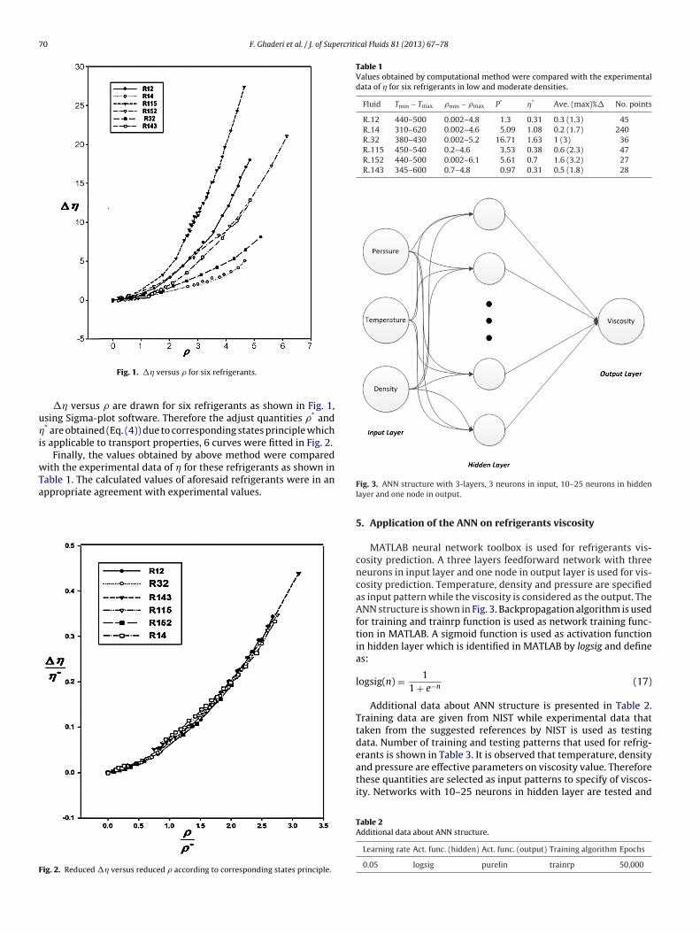
Table 1Values obtained by computational method were compared with the experimentaldata of � for six refrigerants in low and moderate densities.

Fluid Tmin − Tmax �min − �max P* �* Ave. (max)%� No. points

R 12 440–500 0.002–4.8 1.3 0.31 0.3 (1.3) 45R 14 310–620 0.002–4.6 5.09 1.08 0.2 (1.7) 240R 32 380–430 0.002–5.2 16.71 1.63 1 (3) 36R 115 450–540 0.2–4.6 3.53 0.38 0.6 (2.3) 47R 152 440–500 0.002–6.1 5.61 0.7 1.6 (3.2) 27R 143 345–600 0.7–4.8 0.97 0.31 0.5 (1.8) 28

Fig. 1. �� versus � for six refrigerants.

�� versus � are drawn for six refrigerants as shown in Fig. 1,sing Sigma-plot software. Therefore the adjust quantities �* and* are obtained (Eq. (4)) due to corresponding states principle which

s applicable to transport properties, 6 curves were fitted in Fig. 2.Finally, the values obtained by above method were compared

ith the experimental data of � for these refrigerants as shown inable 1. The calculated values of aforesaid refrigerants were in an

ppropriate agreement with experimental values.

ig. 2. Reduced �� versus reduced � according to corresponding states principle.

Fig. 3. ANN structure with 3-layers, 3 neurons in input, 10–25 neurons in hiddenlayer and one node in output.

5. Application of the ANN on refrigerants viscosity

MATLAB neural network toolbox is used for refrigerants vis-cosity prediction. A three layers feedforward network with threeneurons in input layer and one node in output layer is used for vis-cosity prediction. Temperature, density and pressure are specifiedas input pattern while the viscosity is considered as the output. TheANN structure is shown in Fig. 3. Backpropagation algorithm is usedfor training and trainrp function is used as network training func-tion in MATLAB. A sigmoid function is used as activation functionin hidden layer which is identified in MATLAB by logsig and defineas:

logsig(n) = 11 + e−n

(17)

Additional data about ANN structure is presented in Table 2.Training data are given from NIST while experimental data thattaken from the suggested references by NIST is used as testingdata. Number of training and testing patterns that used for refrig-erants is shown in Table 3. It is observed that temperature, density

and pressure are effective parameters on viscosity value. Thereforethese quantities are selected as input patterns to specify of viscos-ity. Networks with 10–25 neurons in hidden layer are tested and

Table 2Additional data about ANN structure.

Learning rate Act. func. (hidden) Act. func. (output) Training algorithm Epochs

0.05 logsig purelin trainrp 50,000

F. Ghaderi et al. / J. of Supercritical Fluids 81 (2013) 67– 78 71

Fig. 4. Viscosity regression comparison between computational and ANN methods for R12. (a) Comparison in high density (d > 5). (b) Comparison in moderate density(2 < d < 5). (c) Comparison in low density (d < 2).

72 F. Ghaderi et al. / J. of Supercritical Fluids 81 (2013) 67– 78

Fig. 5. Viscosity regression comparison between computational and ANN methods for R14. (a) Comparison in high density (d > 5). (b) Comparison in moderate density(2 < d < 5). (c) Comparison in low density (d < 2).

F. Ghaderi et al. / J. of Supercritical Fluids 81 (2013) 67– 78 73

Fig. 6. Viscosity regression comparison between computational and ANN methods for R32. (a) Comparison in high density (d > 5). (b) Comparison in moderate density(2 < d < 5). (c) Comparison in low density (d < 2).

74 F. Ghaderi et al. / J. of Supercritical Fluids 81 (2013) 67– 78

Fig. 7. Viscosity regression comparison between computational and ANN methods for R115. (a) Comparison in high density (d > 5). (b) Comparison in moderate density(2 < d < 5). (c) Comparison in low density (d < 2).

F. Ghaderi et al. / J. of Supercritical Fluids 81 (2013) 67– 78 75

Fig. 8. Viscosity regression comparison between computational and ANN methods for R143. (a) Comparison in high density (d > 5). (b) Comparison in moderate density(2 < d < 5). (c) Comparison in low density (d < 2).

76 F. Ghaderi et al. / J. of Supercritical Fluids 81 (2013) 67– 78

Fig. 9. Viscosity regression comparison between computational and ANN methods for R152. (a) Comparison in high density (d > 5). (b) Comparison in low density (d < 2).

bllwvi

TN

In this study two methods are compared in application ofsix refrigerants viscosity prediction. The computational methodbased on Chapman–Enskog and Rainwater–Friend theories is a

est network is specified. Table 4 is devoted to exhibition of corre-ation value (R) of networks and computational method for R12 inow and moderate densities. These results denote that a network

ith 20 neuron in hidden layer show very acceptable values foriscosity in agreement with experimental values. This agreement

s observed in all range of densities as shown in Table 5 and Figs. 4–9.

Figure 8.

able 3umber of training and testing patterns in ANN for refrigerants.

Fluid No. of training patterns No. of testing patterns

R12 1170 56R14 341 59R32 161 54R115 217 55R143 174 59R152 213 72

6. Discussion

Table 4R values for R12 in low and moderate densities. Comparison between computationalmethod and 16 artificial neural network structures.

Method R value Method R value

Computational 0.99983 ANN, 18 hidden nodes 0.996795ANN, 10 hidden nodes 0.992646 ANN, 19 hidden nodes 0.991328ANN, 11 hidden nodes 0.996801 ANN, 20 hidden nodes 0.999778ANN, 12 hidden nodes 0.985168 ANN, 21 hidden nodes 0.999635ANN, 13 hidden nodes 0.996069 ANN, 22 hidden nodes 0.988639ANN, 14 hidden nodes 0.990111 ANN, 23 hidden nodes 0.811830ANN, 15 hidden nodes 0.997962 ANN, 24 hidden nodes 0.971865ANN, 16 hidden nodes 0.994237 ANN, 25 hidden nodes 0.984178ANN, 17 hidden nodes 0.999607

F. Ghaderi et al. / J. of Supercriti

Table 5R values for six refrigerants in low, moderate and high density. Comparison betweenANN approach and computational method.

Fluid ANN method R values Computational method R valuesLow d Moderate d High d Low d Moderate d High d

R12 0.9616 0.9998 0.9997 0.9984 0.9991 0.9931R14 0.9994 0.9951 0.9995 0.9983 0.9825 −0.9943R32 0.9989 0.9995 1 0.9993 0.9995 −0.9991R115 0.9892 0.9973 0.9906 0.9997 0.9993 0.9054R143 0.9950 0.9998 0.9998 0.9998 0.9999 0.9535R152 0.9949 – 0. 9758 0.9718 – 0.9268

Table 6R values for six refrigerants in all range of densities. Comparison between ANNapproach and computational method.

Fluid Density range ANN R value Computational R value

R12 d < 8 0.99975 0.99934R14 d < 20 0.99911 −0.61345R32 d < 27 1 −0.99525R115 d < 11.5 0.99744 0.95915R143 d < 15.5 0.99995 0.97823R152 d < 18 0.98203 −0.91009

sdiichciadftSaaamp

7

dapiile

pRptf

faa

[

[

[

[

[

[

[

[

[

[

[

[

[

[

[24] A.H. Ghaderi, A.H. Darooneh, Artificial neural network with regular graph formaximum air temperature forecasting: the effect of decrease in nedes degreeon learning, International Journal of Modern Physics C 23 (2012) 1–10.

[25] G. Li, J. Shi, On comparing three artificial neural networks for wind speed fore-

tatistical method for viscosity prediction in low and moderateensities. But in higher densities this method is failed as shown

n Figs. 5a, 6a, 7a, 9a, and 10a and Table 5 for R14, R32, R152. Ast is indicated in Table 6, for densities higher than 8, accuracy ofomputational methods will become less and less. On the otherand ANN method is a nonlinear method that is applied for vis-osity prediction in a wide range of density and temperature. Ast is represented in Figs. 4–9 and Tables 5, 6 this method is valu-ble for viscosity prediction. Table 6 is exploring R = 1 for R32 atensities close to 27 while in computational method R = −0.99525or this fluid. This result is apparent for R152 and R14 where densi-ies are close to 20. But ANN method is limited by some hinders.ince training step in ANN needs many training patterns for a suit-ble test, viscosity of refrigerants in specific densities, pressuresnd temperatures should be determined for training before testingnd this is a disadvantage of ANN method versus computationalethods. The number of training and testing patterns for viscosity

rediction of six refrigerants in ANN method is shown in Table 3.

. Conclusion

We found that ANN approach in moderate and high range ofensity is reliable as low densities, while computational methodsre restricted in densities less than 8. Table 5 certificates that com-utational method is a reliable approach for viscosity prediction

n low density (d < 2) and moderate density (2 > d > 5) for six flu-ds and even some higher densities for R12 where density range isower than 8 (see Table 6). Performance of the two methods also isxplored in Figs. 4–9.

Finally according to the results of low density ranges, com-utational methods based on Chapman–Enskog relation andainwater–Friend theory are very accurate methods for viscosityrediction. However, since this accuracy is reduced in higher densi-ies, feedforward neural network as a nonlinear method is proposedor solving this problem.

Other nonlinear methods such as neuro-fuzzy may be usedor viscosity and other transport properties prediction as reliablepproaches. Neuro-fuzzy may be used for better and faster learning

nd prediction in transport properties prediction.

cal Fluids 81 (2013) 67– 78 77

Acknowledgements

The authors of this paper present a special thanks to NISTChemistry WebBook at http://webbook.nist.gov/chemistry/ includ-ing references and useful data for training neural networks. We arealso grateful to the anonymous reviewers for excellent commentsand suggestions.

Appendix A. Supplementary Data

Supplementary data associated with this article can befound, in the online version, at doi:http://dx.doi.org/10.1016/j.supflu.2013.04.017.

References

[1] S.G. Penoncello, R.T. Jacobsen, E.W. Lemmon, A fundamental equation fordichlorodifluoromethane (R-12), Fluid Phase Equilibria 80 (1992) 57–70.

[2] R.G. Rubio, J.C.G. Calado, P. Clancy, W.B. Streett, A theoretical and experimen-tal study of the equation of state of tetrafluoromethane, Journal of PhysicalChemistry 89 (1985) 4637–4646.

[3] J.H. Smith, E.L. Pace, Thermodynamic properties of carbon tetrafluoride from 12.deg. K to its boiling point. Significance of the parameter. nu, Journal of PhysicalChemistry 73 (1969) 4232–4236.

[4] S.B. Kiselev, R.A. Perkins, M.L. Huber, Transport properties of refrigerants R32,R125, R134a, and R125+R32 mixtures in and beyond the critical region, Inter-national Journal of Refrigeration 22 (1999) 509–520.

[5] T. Makita, Thermophysical properties of liquids at high pressures, InternationalJournal of Thermophysics 5 (1984) 23–40.

[6] R. Krauss, V.C. Weiss, T.A. Edison, J.V. Sengers, K. Stephan, Transport proper-ties of 1,1-difluoroethane (R152a), International Journal of Thermophysics 17(1996) 731–757.

[7] I.N. Levine, Physical Chemistry, McGraw-Hill, New York, 1995.[8] B. Najafi, E.A. Mason, J. Kestin, Improved corresponding states principle for the

noble gases, Physica A 119 (1983) 387–440.[9] B. Najafi, Y. Ghayeb, G.A. Parsafar, New correlation functions for viscosity cal-

culation of gases over wide temperature and pressure ranges, InternationalJournal of Thermophysics 21 (2000) 1011–1031.

10] J.C. Rainwater, D.G. Friend, Second viscosity and thermal-conductivity virialcoefficients of gases: extension to low reduced temperature, Physical ReviewA 36 (1987) 4062–4066.

11] R.A. Aziz, A highly accurate interatomic potential for argon, Journal of ChemicalPhysics 99 (1993) 4518–4526.

12] B. Najafi, Y. Ghayeb, J.C. Rainwater, S. Alavi, R.F. Snider, Improved initial den-sity dependence of the viscosity and a corresponding states function for highpressures, Physica A 260 (1998) 31–48.

13] B. Najafi, R. Araghi, J.C. Rainwater, S. Alavi, R.F. Snider, Prediction of the ther-mal conductivity of gases based on the Rainwater–Friend theory and a newcorresponding states function, Physica A 275 (2000) 48–69.

14] H. Behnejad, M.S. Miralinaghi, Initial density dependence of the viscosity ofhydrogen and a corresponding states expression for high pressures, Journal ofMolecular Liquids 113 (2004) 143–148.

15] F.S. Hashemi, S.S. Tafreshi, Calculation of the viscosity of simple fluids basedon the Rainwater–Friend theory, Journal of the Chinese Chemical Society 54(2007) 9–14.

16] J. Millat, J.H. Dymond, C.A. Nieto de Castro, Transport Properties of Fluid,Cambridge University Press, Cambridge, 1996.

17] A. Sozen, M. Ozalp, E. Arcaklioglu, Investigation of thermodynamic proper-ties of refrigerant/absorbent couples using artificial neural networks, ChemicalEngineering and Processing: Process Intensification 43 (2004) 1253–1264.

18] A. Mohebbi, M. Taheri, A. Soltani, A neural network for predicting saturatedliquid density using genetic algorithm for pure and mixed refrigerants, Inter-national Journal of Refrigeration 31 (2008) 1317–1327.

19] A. Sencana, S.A. Kalogiroub, A new approach using artificial neural networksfor determination of the thermodynamic properties of fluid couples, EnergyConversion and Management 46 (2005) 2405–2418.

20] Y.H. Hu, J. Hwang, Handbook of Neural Network Signal Processing, CRC Press,Boca Raton, 2001.

21] Z.H. Zhou, J. Wu, W. Tang, Ensembling neural networks: many could be betterthan all, Artificial Intelligence 137 (2002) 239–263.

22] J. Wu, J. Kuo, An automotive generator fault diagnosis system using discretewavelet transform and artificial neural network, Expert Systems with Applica-tions 36 (2009) 9776–9783.

23] M.V. Ramrez, H.F. de Campos Velho, N.J. Ferreira, Artificial neural networktechnique for rainfall forecasting applied to the Sao Paulo region, Journal ofHydrology 301 (2005) 146–162.

casting, Applied Energy 87 (2010) 2313–2320.

7 ercriti

[

[

[

[

[

[

[

[

[

[

[

[

[

[

[

[

[

[

[

[

[

[

[

[

[

[

[

[

[

[

[

[

[

[

[

[

[

[

[

[

[

[

[

[

[

[

[

[[74] F. Rosenblatt, The perceptron: a probabilistic model for information storage

8 F. Ghaderi et al. / J. of Sup

26] H. Selim, Determinants of house prices in Turkey: hedonic regressionversus artificial neural network, Expert Systems with Applications 36 (2009)2843–2852.

27] A. Sozen, Future projection of the energy dependency of Turkey using artificialneural network, Energy Policy 37 (2009) 4827–4833.

28] E. Arcaklioglu, A. Cavusoglu, A. Erisen, Thermodynamic analyses of refrigerantmixtures using artificial neural networks, Applied Energy 78 (2004) 219–230.

29] N. Austin, P. Senthilkumar, S. Purushothaman, Mixed refrigerants suitabilityanalysis using artificial neural networks, ARPN Journal of Engineering andApplied Sciences 7 (2012) 588–592.

30] G. Scalabrin, C. Corbetti, G. Cristofoli, A viscosity equation of state for r123 inthe form of a multilayer feedforward neural network, International Journal ofThermophysics 22 (2001) 1383–1395.

31] G. Cristofoli, L. Piazza, G. Scalabrin, A viscosity equation of state for R134athrough a multi-layer feedforward neural network technique, Fluid PhaseEquilibria 199 (2002) 223–236.

32] A. Sozen, E. Arcaklioglu, T. Menlik, Derivation of empirical equations for ther-modynamic properties of a ozone safe refrigerant (R404a) using artificial neuralnetwork, Expert Systems with Applications 37 (2010) 1158–1168.

33] A. Sozen, M. Ozalp, E. Arcaklioglu, Calculation for the thermodynamic prop-erties of an alternative refrigerant (R508b) using artificial neural network,Applied Thermal Engineering 27 (2007) 551–559.

34] C. Coquelet, F. Rivollet, C. Jarne, A. Valtz, D. Richon, Measurement of physicalproperties of refrigerant mixtures. Determination of phase diagrams, EnergyConversion and Management 47 (2006) 3672–3680.

35] D.V. Singh, G. Maheshwari, R. Shrivastav, D.K. Mishra, Neural network – com-paring the performances of the training functions for predicting the value ofspecific heat of refrigerant in vapor absorption refrigeration system, Interna-tional Journal of Computer Applications 18 (2011) 1–5.

36] V.Z. Geller, S.D. Artamonov, G.V. Zaporozhan, V.G. Peredrii, Thermal conductiv-ity of freon-12, Journal of Engineering Physics and Thermophysics 27 (1974)842–846.

37] F.G. Keyes, Thermal conductivity of gases, Transactions of the American Societyof Mechanical Engineers 76 (1954) 809–816.

38] T. Makita, Y. Tanaka, Y. Morimoto, M. Noguchi, H. Kubota, Thermal conductivityof gaseous fluorocarbon refrigerants R12, R13, R22, and R23 under pressure,International Journal of Thermophysics 2 (1981) 249–268.

39] J.E.S. Venart, N. Mani, The thermal conductivity of R12, Transactions of theCanadian Society for Mechanical Engineering 3 (1975) 1–9.

40] J. Yata, T. Minamiyama, S. Tanaka, Measurement of thermal conductivity ofliquid fluorocarbons, International Journal of Thermophysics 5 (1984) 209–218.

41] M.J. Assael, E. Karagiannidis, W.A. Wakeham, Measurements of the thermalconductivity of R11 and R12 in the temperature range 250–340 K at pressuresup to 30 MPa, International Journal of Thermophysics 13 (1992) 735–751.

42] A.S. Rodgers, J. Chao, R.C. Wilhoit, B.J. Zwolinski, Ideal gas thermodynamic prop-erties of eight chloro- and fluoromethanes, Journal of Physical and ChemicalReference Data 3 (1974) 117–140.

43] M.O. McLinden, S.A. Klein, R.A. Perkins, An extended corresponding statesmodel for the thermal conductivity of refrigerants and refrigerant mixtures,International Journal of Refrigeration 23 (2000) 43–63.

44] N. Imaishi, J. Kestin, R. Paul, Thermal conductivity of carbon tetrafluoride withargon and helium, International Journal of Thermophysics 6 (1985) 3–20.

45] S. Oshen, B.M. Rosenblum, G. Thodos, Thermal conductivity of carbon tetraflu-oride in the dense gaseous region, Journal of Chemical Physics 46 (1967)2939–2944.

46] B.M. Rosenbaum, G. Thodos, Thermal conductivity of mixtures in the densegaseous state: the methane–carbon tetrafluoride system, Physica (Amsterdam)37 (1967) 442–456.

47] J. Millat, M. Ross, W.A. Wakeham, M. Zalaf, The thermal conductivity of neon,methane and tetrafluoromethane, Physica (Amsterdam) 148A (1988) 124–152.

48] G.V. Zaporozhan, V.Z. Geller, Experimental investigation of the thermal con-ductivity coefficient of freons R-13 and R-14 at low temperature, Zhurnalfizicheskoi khimii 51 (1977) 1056–1059.

49] G.C. Maitland, E.B. Smith, Viscosities of binary gas mixtures at high tem-

peratures, Journal of the Chemical Society, Faraday Transactions 1: PhysicalChemistry in Condensed Phases 70 (1974) 1191–1211.

50] J. Kestin, H.E. Khalifa, S.T. Ro, W.A. Wakeham, The viscosity of diffusioncoefficients of eighteen binary gaseous systems, Physica (Amsterdam) 88A(1977) 242–260.

[

[

cal Fluids 81 (2013) 67– 78

51] K. Marsh, R. Perkins, M.L.V. Ramires, Measurement and correlation of the ther-mal conductivity of propane from 86 to 600 K at pressures to 70 MPa, Journalof Chemical & Engineering Data 47 (2002) 932–940.

52] B. Le Neindre, Y. Garrabos, Measurement of thermal conductivity of HFC-32 (difluoromethane) in the temperature rante from 300 to 465 K atpressures up to 50 MPa, International Journal of Thermophysics 22 (2001)701–722.

53] X. Gao, H. Iojima, Y. Nagasaka, A. Nagashima, Thermal conductivity of HFC-32 in the liquid phase, in: Proceedings 4th Asian Thermophysical PropertiesConference (Paper C1c4), Tokyo, 1995.

54] S.T. Ro, J.W. Kim, D.S. Kim, Thermal conductivity of R32 and its mixture withR134a, International Journal of Thermophysics 16 (1995) 1193–1201.

55] M. Papadaki, W.A. Wakeham, Thermal conductivity of R32 and R125 in theliquid phase at the saturation vapor pressure, International Journal of Thermo-physics 14 (1993) 1215–1220.

56] M.J. Assael, L. Karagiannidis, Measurements of the thermal conductivity of liq-uid R32, R124, R125, R141b, International Journal of Thermophysics 16 (1995)851–865.

57] U. Gross, Y.W. Song, Thermal conductivities of new refrigerants R125 and R32measured by the transient hot-wire method, International Journal of Thermo-physics 17 (1996) 607–619.

58] J. Yata, M. Hori, K. Kobayashi, T. Minamiyama, Thermal conductivity of alter-native refrigerants in the liquid phase, International Journal of Thermophysics17 (1996) 561–571.

59] E. Hahne, U. Gross, Y.W. Song, The thermal conductivity of R115 in the criticalregion, International Journal of Thermophysics 10 (1989) 687–700.

60] J. Yata, T. Minamiyama, S. Tanaka, Measurement of thermal conductivity ofliquid fluorocarbons, International Journal of Thermophysics 5 (1984) 209–218.

61] V.Z. Geller, Investigation of the viscosity of freons of the methane, ethane, andpropane types. Summary of experimental data, Teplofizika Svoistva VestchestvMater 15 (1980) 89–114.

62] V. Vesovic, W.A. Wakeham, G.A. Olchowy, J.V. Sengers, J.T.R. Watson, J. Millat,The transport properties of carbon dioxide, Journal of Physical and ChemicalReference, Data 19 (1990) 763–808.

63] B. Haghighi, F. Heidari, M.M. Papari, Viscosity prediction for R32 and R143aat moderate density regimes via semi-empirically based assessment, IndianJournal of Chemistry. Section A, Inorganic, Bio-inorganic, Physical, Theoretical& Analytical Chemistry 47 (2008) 867–874.

64] J.W. Schmidt, E. Carrillo-Nava, M.R. Moldover, Partially halogenated hydrocar-bons CHFCl–CF3, CF3–CH3, CF3–CHF–CHF2, CF3–CH2–CF3, CHF2–CF2–CH2F,CF3–CH2–CHF2, CF3–O–CHF2: critical temperature, refractive indices, surfacetension and estimates of liquid, vapor and critical densities, Fluid Phase Equilib-ria 122 (1996) 187–206.

65] J. Bzowski, J. Kestin, E.A. Mason, F.J. Uribe, Equilibrium and transport propertiesof gas mixtures at low density: eleven polyatomic gases and five noble gases,Journal of Physical and Chemical Reference Data 19 (1990) 1179–1232.

66] R. Krauss, V.C. Weiss, T.A. Edison, J.V. Sengers, K. Stephan, Transport proper-ties of 1,1-difluoroethane (R152a), International Journal of Thermophysics 17(1996) 731–757.

67] P.S. van der Gulik, The viscosity of the refrigerant 1,1-difluoroethane along thesaturation line, International Journal of Thermophysics 14 (1993) 851–864.

68] J.O. Felder, C.F. Curtiss, R.B. Bird, Molecular Theory of Gases and Liquids, Wiley,New York, 1964.

69] H. O’Hara, F.J. Smith, Transport collision integrals for a dilute gas, ComputerPhysics Communications 2 (1971) 47–54.

70] J.C. Rainwater, Softness expansion of gaseous transport properties. II. Moder-ately dense gases, Journal of Chemical Physics 74 (1981) 4130–4144.

71] J.C. Rainwater, On the phase space subdivision of the second virial coefficientand its consequences for kinetic theory, Journal of Chemical Physics 81 (1984)495–511.

72] G. Dreyfus, Neural Networks: Methodology and Applications, Springer, Berlin,2005.

73] W.H. Steeb, The Nonlinear Workbook, World Scientific, New York, 2005.

and organization in the brain, Psychological Review 65 (1958) 386–408.75] S. Haykin, Neural Networks: A Comprehensive Foundation, IEEE, New York,

1999.76] L. Fausett, Fundamentals of Neural Networks, Prentice Hall, NJ, 1994.