Vector autoregressive models versus neural networks in forecasting: an application to Euro-inflation...

1

A Comparison of Linear Forecasting Models and Neural Networks: An Application to Euro inflation and Euro Divisia

Short title: Linear Models versus Neural Networks in Macroeconomic Forecasting

Jane M. Binner (corresponding author)

Department of Information Management and Systems Nottingham Business School Nottingham Trent University Nottingham, NG1 4BU, UK

Email: [email protected] Tel: +44 (0) 115 848 2429 Fax: +44 (0) 115 848 6175

Rakesh K. Bissoondeeal



Thomas Elger

Department of Economics Lund University P. O. Box 7082 Lund, Sweden

Email: [email protected] Tel: +46 46 222 7919 Fax: +46 46 222 4118

Alicia M. Gazely



Andrew W. Mullineux

Department of Accounting and Finance Birmingham Business School

The University of Birmingham Birmingham, B15 2TT, UK


2

Abstract Linear models reach their limitations with nonlinearities in the data. This paper provides new empirical evidence on the relative macroeconomic forecasting performance of linear and nonlinear models. The well established and widely used univariate autoregressive integrated moving average (ARIMA) and multivariate vector autoregressive (VAR) models are used as linear forecasting models whereas neural networks (NN) are used as nonlinear forecasting models. We endeavour to keep the level of subjectivity in the NN building process to a minimum in an attempt to exploit its full capability. This paper also investigates whether the historically poor performance of the theoretically superior measure of the monetary services flow, Divisia, relative to the traditional Simple Sum measure could be attributed to a certain extent to the evaluation of these indices within a linear framework. The results obtained suggest that nonlinear models provide better within-sample and out-of-sample forecasts and linear models are simply a subset of them. The Divisia index also outperforms the Simple Sum index when evaluated in a nonlinear framework. 1. Introduction This paper is concerned with forecasting the inflation rate in the Euro area. Nonlinear NN are compared to the more traditional time series univariate ARIMA and multivariate VAR forecasting models. The objectives are two-fold: (1) Primarily to display how various time series forecasting methods compare in their forecasting accuracy of Euro inflation. (2) Secondly, given the ubiquitous relationship between inflation and money, to compare the inflation forecasting ability of the Euro M3 and a Euro Divisia M3 in both linear and nonlinear frameworks. The reason for carrying out such an empirical analysis is that it can provide useful information to monetary policy decision makers of the ECB whose primary objective is to maintain price stability in the Euro area. The ECB organises its assessment of risks of price stability under two pillars (see ECB, 1999a, b and 2000). Firstly, given the widely held belief that development in the price level is a monetary phenomenon, development in the amount of money held by the public may reveal useful information about future price development and be a useful leading indicator of inflation. Therefore in 1998, in its first pillar of monetary policy strategy, the ECB decided to give broad monetary aggregate Euro M3 a prominent role. The second pillar analyses a broad range of other economic and financial time series indicators relevant to future price developments. Our first objective is particularly relevant to the second pillar of the ECB’s monetary policy strategy where inflation forecasts play a very important role. In order to enable the monetary authorities to tackle appropriately inflationary pressures that may arise in the future it is necessary and crucial to produce accurate and reliable forecasts of inflation. A large body of research is devoted to inflation forecasting (see, for example, De Brouwer and Ericsson, (1998) for Australia, Stock and Watson (1999) for the US, Drake and Mills (2002) for the Euro area). One question that lies in the heart of every forecasting exercise is which forecasting method to use? The overwhelming majority of studies on inflation forecasting divide forecasts in 2 main categories (1) forecasts from time series models such as ARIMA models and (2) forecasts from macroeconomic models such as the VAR models.

3

However, such models are based on the assumption of linearity in the data and there is now growing evidence that macroeconomic series contain nonlinearities (see for example, Tiao and Tsay (1994) and Stanca (1999) and thus, though linear models have been reasonably successful as a practical tool for analysis and forecasting, they are inherently limited in the presence of nonlinearities in data and consequently forecasts, as well as other conclusions drawn, from them could be misleading. In view of the limitations of the linear models, nonlinear time series have gained much attention in the recent decades. Several nonlinear models, such as the threshold autoregressive (TAR) models (Tong, 1990) and the exponential autoregressive model (EXPAR) (Haggan and Ozaki, 1981), have been developed. However, an immediate problem encountered while opting for such nonlinear models in preference to linear models is that there exists no unified theory that can be applied to all such nonlinear models as they require the imposition of assumptions concerning the precise form of nonlinearity. But there are too many possible nonlinear patterns in a particular data set and the prespecified nonlinear model may not be broad enough to capture all essential characteristics. An alternative way to deal with nonlinearities in data is to use NN. In contrast to the above model-based nonlinear methods, NN are data driven and are thus capable of producing nonlinear models without prior beliefs about the functional forms. NN are also highly flexible as they can approximate any continuous function to any degree of accuracy (Hornik et al., 1989). Thus from a statistical viewpoint the nonlinear NN would be expected to perform better than the linear models in inflation forecasting and since no such work has been carried out for the Euro area we investigate the performance of NN vis a vis linear models in forecasting Euro inflation. In the first pillar of the ECB’s monetary policy strategy, Euro M3, constructed by simple summation, plays a very important role (see ECB 1999a,b, 2000 for more details). However, there is some debate (see, Barnett, 1980, 1982) that monetary aggregates constructed by simple summation are flawed and the weighted Divisia monetary aggregates are a theoretically superior measure of monetary services flow and hence Drake et al. (1997) among others have suggested the use of a Euro Divisia M3 instead of Euro M3 in the first pillar of the ECB’s monetary policy strategy. However, despite its theoretical superiority the Divisia index does not always outperform its Simple Sum counterpart empirically (Chrystal and MacDonald, 1994, Herrmann et al., 2000), explaining the reluctance of the ECB and other central banks in adopting such a monetary index for their monetary policy strategy. To provide an explanation for the historically poor performance of the Divisia index, researchers have focussed on measurement problems (see for example Drake et al., 1997). However, none of them have put the validity of the linear statistical methods used to evaluate them into question despite the fact that, as stated earlier, there is increasing evidence of nonlinearity in macroeconomic data and more importantly the fact that Barnett and Chen (1986, 1988a, b), Barnett and Hinich (1992, 1993), Chen (1988), and DeCoster and Mitchell (1991) have provided evidence of nonlinear structures inherent in the Divisia index. Thus if the Divisia index performs poorly relative to the Simple Sum index when compared in a linear framework one cannot say whether it is the Divisia index to be blamed or the linear models which may not be able to capture nonlinear behaviour. Given the ubiquitous relationship between inflation and monetary aggregates this study can therefore be used to shed some light on the issue of whether the historical poor performance of the Divisia index relative its Simple

4

Sum counterpart could be attributed to a certain extent to incorrectly using linear statistical models in evaluating them. More specifically, we construct multivariate linear and nonlinear forecasting models and interchange Euro M3 and Euro Divisia M3 to investigate their comparative forecasting performance. Hence this study allows us to evaluate the forecasting potentials of linear univariate and multivariate models and nonlinear NN in predicting Euro inflation and to compare the relative performance of Euro M3 and Euro Divisia M3 in linear and nonlinear frameworks. This paper is organised as follows: The next section provides a brief review of the literature comparing linear and nonlinear forecasting models. Section 3 describes the data and associated preliminary analysis. In section 4 the different models are specified and estimated. Forecasts results are presented and discussed in section 5 while conclusions and suggestions for future development are offered in section 6. 2. Literature Comparing Forecasting Method Effectiveness This section attempts to provide a brief review of recent research on comparing linear models, like ARIMA and VAR models to nonlinear NN, but makes no attempt to be exhaustive. NN have gained enormous popularity in the recent years, especially in time series forecasting. Most applications, however, are in areas where data are abundant as NN are very data intensive. In macroeconomics, due to the scarcity of large data samples, there exists only a few studies involving the use of NN that can be used to gauge its usefulness in the field. Recent ones include that of Johnes (2000) and Moshiri and Cameron (2000). Johnes (2000) contrasts models of the UK economy constructed using NN and a variety of econometric models. Moshiri and Cameron (2000) use NN to forecast Canadian inflation and compare the results to those from time series and econometric models. The results in these studies, based on out-of-sample forecasts, do not permit a demarcation between the linear models and NN as the latter is able to justify its theoretical superiority in only some of the cases. In fact, these observations reflect the results of quite a large number of such comparative studies across different fields. This has led to questions being raised on whether studies implement NN in such a way that it stands a reasonable chance of performing well (Adya and Callopy, 1998). Indeed, the risks of making bad decisions are extremely high while building a NN as there are no established procedures available to decide on the choice of the parameters of the NN, which basically is problem dependent. Although there have been attempts in several studies to develop guidelines in making these choices (see, for example, Balkin and Ord (2000), Gorr et al. (1994)), so far this matter, is still subject to trial and error. Thus, despite the many satisfactory characteristics of the NN, building a NN for forecasting a particular problem is a nontrivial task. Consequently, tedious experiments and time-consuming trial and error procedures are inevitable. However, this has not been the case in most of the comparative studies as in the absence of any a priori information about the parameters of the NN, their choice has involved a lot of subjectivity (Nag and Mitra, 2002). Such an approach considerably reduces the possibilities of exploiting the true potentials of the NN and ultimately leads to results from a large number of studies being dubious. For example, Moshiri and Cameron (2000) perform some experimentation in finding the optimum number of hidden units, however their choice for the amount of training required, another equally critical parameter, is rather subjective, thereby limiting the power of the NN. In this study, we endeavour to keep the level of subjectivity to a minimum

5

and appropriately deal with other issues prone to affect the performance of NN in an attempt to obtain the best possible NN models. Since it is beyond our reach to evaluate the performance of NN against the entire class of linear models, we chose the well-established and extensively used ARIMA and VAR models as our representatives for linear models in recognition of their ability to produce reliable forecasts. 3. Data and Preliminary Analysis Many economic indicators help predict inflation. For example Stock and Watson (1999) have recently shown that 168 variables can be used to forecast US inflation. In our study instead of using so many variables, we limit the list of variables to those that are more closely linked to inflation by economic theory or that have been regularly used in previous empirical studies. Thus, in keeping with previous studies such as Hendry and Doornik (1994) and Lutkepohl and Wolters (1998)), the variables required for multivariate forecasting are: inflation, monetary aggregates- Euro M3 and Euro Divisia M3, GDP, GDP deflator and the opportunity cost variables of the corresponding Divisia and the Simple Sum aggregates. These are quarterly seasonally adjusted data, for the period 1980Q1 to 2000Q4, defined by the availability of the Euro-area data. Data on monetary assets, their respective rates of return, GDP and GDP deflator have been obtained from Stracca (2001). After allowing for lags and transformations estimation is conducted using data from 1981Q2 to 1998Q2, while the remaining 10 observations (1998Q3 to 2000Q4) are kept for forecast evaluation (testing). The Simple Sum index is constructed by simply summing over the monetary components while the Divisia index is constructed using equation (9) in Barnett et al. (1992, pp. 2097). We use the Divisia price dual (Barnett, 1980) as the opportunity cost variable for Divisia. Following Lutkephol and Wolters (1998) the opportunity cost variable for the Simple Sum aggregate is calculated as )( tt rR − where tR is a long term interest rate and tr is the own rate of M3. The log of all variables have been taken and thus tm3 is the log of real Simple Sum M3, td3 is log of real Euro Divisia M3, ty is the log of real GDP, tdualm3 is the log of the opportunity cost variable for Euro M3 and tduald3 is the log of the opportunity cost variable for Euro Divisia M3.

tp is the logarithm of the GDP deflator and 1−−=∆ ttt ppp is the quarterly inflation rate.

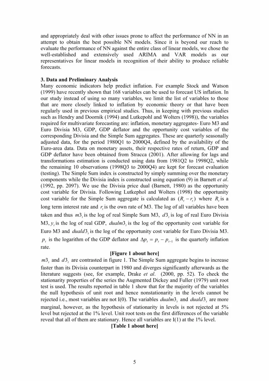
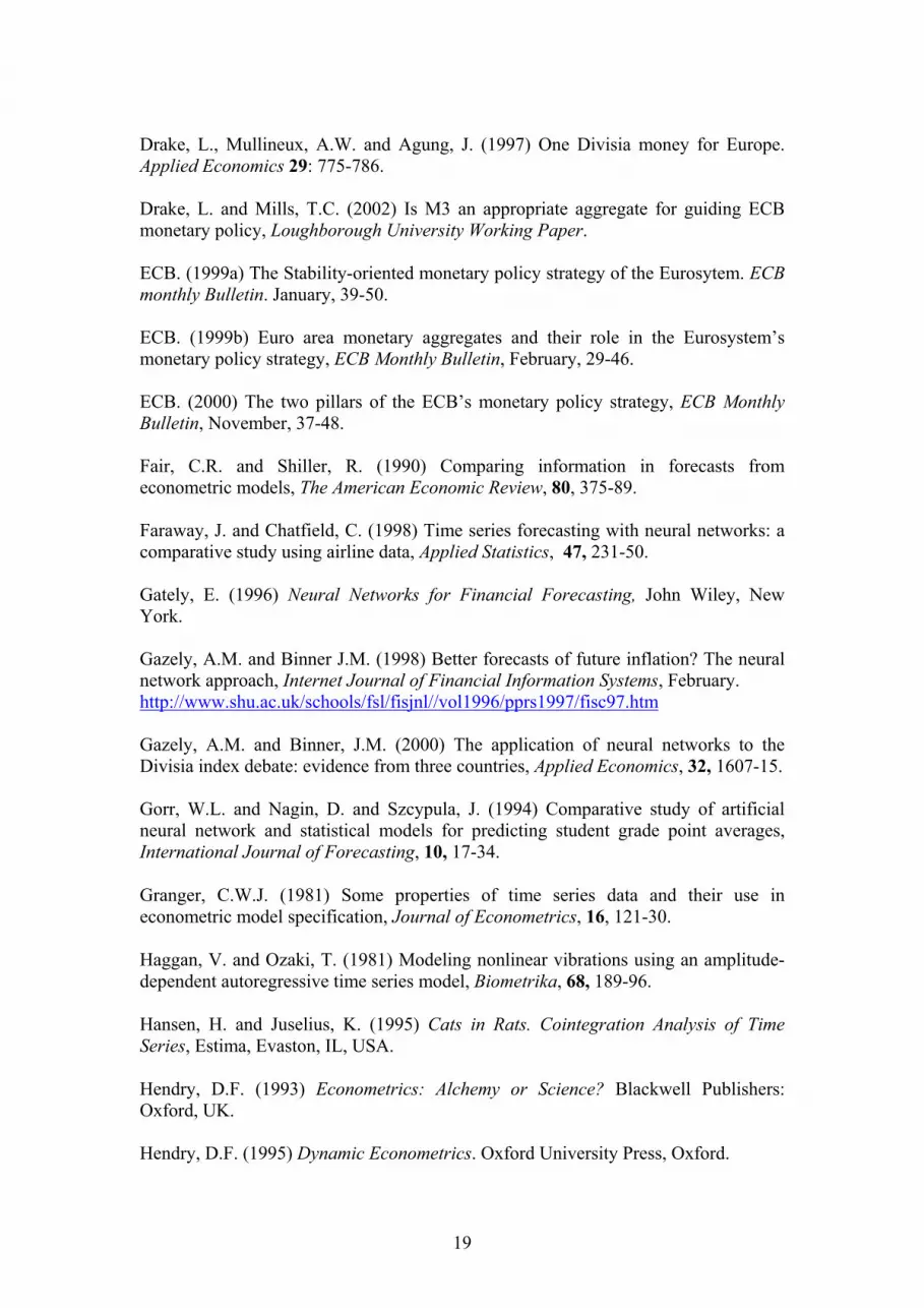
[Figure 1 about here] tm3 and td3 are contrasted in figure 1. The Simple Sum aggregate begins to increase

faster than its Divisia counterpart in 1980 and diverges significantly afterwards as the literature suggests (see, for example, Drake et al. (2000, pp. 52). To check the stationarity properties of the series the Augmented Dickey and Fuller (1979) unit root test is used. The results reported in table 1 show that for the majority of the variables the null hypothesis of unit root and hence nonstationarity in the levels cannot be rejected i.e., most variables are not I(0). The variables tdualm3 and tduald3 are more marginal, however, as the hypothesis of stationarity in levels is not rejected at 5% level but rejected at the 1% level. Unit root tests on the first differences of the variable reveal that all of them are stationary. Hence all variables are I(1) at the 1% level.

[Table 1 about here]

6

4. Model Specification and Estimation In this section we present our main decisions regarding the specification and estimation of the three classes of models (univariate ARIMA, multivariate VAR and NN). While the ARIMA and VAR methods are widely used, the NN method is a relatively new method. Thus, we provide only brief accounts for the ARIMA and VAR methods and we give a more detailed account for the NN method. 4.1 Univariate Time Series Model The ARIMA is a general class of univariate time series models which represents current values of a time series by past values of itself (autoregressive term (AR)) and past values of stochastic errors (moving average terms (MA)). The acronym I refers to the number of times (d) the time series has to be differenced to render it stationary. A nonseasonal1 ARIMA(p,d,q) process can be represented as tt

d LyLL εθδφ )()1)(( +=− (1) where tε is independent and normally distributed with zero mean constant variance and δ is a constant. )(Lφ and )(Lθ are the AR and MA polynomials, respectively with orders p and q such that p

p LLL φφφ −−−= L11)( and q

q LLL θθθ −−−= L11)( , where L represents the backshift operator such that

stts yyL −= . A slightly modified Box and Jenkins approach (Box and Jenkins, 1970)

is used for identifying the best model for ARIMA forecasting. Thus, instead of inspecting ACF and PACF in the identification stage we estimate a range of models, represented in table 2, with 2=d ( for tp from section 3) and values of p and q varying from 0 to 3 in a first step and retain the models which pass the diagnostic tests (no autocorrelation and conditional heteroscedasticity, significance of parameters). In a second step the best ARIMA model is chosen to be the one which provides the best out-of-sample forecast. We also estimate an ARIMA model with the orders of p and q equal to 6. We then use Hendry’s (1993) general-to-specific methodology to obtain a more parsimonious model.

[Table 2 about here] Thus after the first step only 4 ARIMA models were retained as the others exhibit insignificant parameters and out of the 4 remaining models the ARIMA(0,2,1) is our preferred ARIMA specification because it outperforms the others in terms of out-of-sample forecasting accuracy. The estimated model2 is given below and the test statistics given are computed from the residuals of the estimated models3. JB represents the Jarque-Bera test for normality, LM(k), represents the test for autocorrelation of order k, and ARCH(k) representing the test for conditional heteroscedasticity of order k (for more details on this tests, see for example, Hendry (1995)). None of the diagnostic tests is significant at conventional levels and, hence, the residuals appear to be normally distributed and free from autocorrelation and autoregressive conditional heteroscedasticity.

( )102.0

510.0)1( 12

−−=− tttpL εε (2)

)92.0(16.0.23.02 == BJR S.E. of regression = 0.002525

LM (1) = 0.00 (1.00) LM (4) = 1.61 (0.81) LM (8) = 4.91(0.77)

ARCH (1) = 0.40 (0.52) ARCH (4) = 7.28 (0.12) ARCH (8) = 10.81(0.21)

7

4.2 Multivariate Vector Autoregressive (VAR) Models The advantage of VAR models over ARIMA models is that they can incorporate more information in terms of other time series instead of just past observations and errors of the series to be forecast. Having established in section 3 that the variables entering the VAR are I(1), we first proceed to investigate whether they are cointegrated, that is, verify whether some linear combination of these nonstationary variables is stationary. In the absence of cointegration between the variables a common forecasting procedure would be to conduct a VAR on the first differences. However, if cointegrating relationships can be established between the variables, the VAR should also include the lagged cointegrating error term (vector error correction models (VECM)) (Granger, 1981). This prevents neglecting long run information contained in the levels of the variables and it has been shown that such an approach leads to improved forecasting accuracy (Lesage(1990), Shoesmith (1992, 1995)). 4.2.1 Testing for Cointegration To check for cointegration, the Johansen (1988) procedure is used. Thus let tz be a

1×q vector, here Tt

opptttt pRyMz ),,,( ∆= where tt mM 3= / td3 and

ttoppt dualddualmR 3/3= then tz can be formulated as the first difference of a VAR

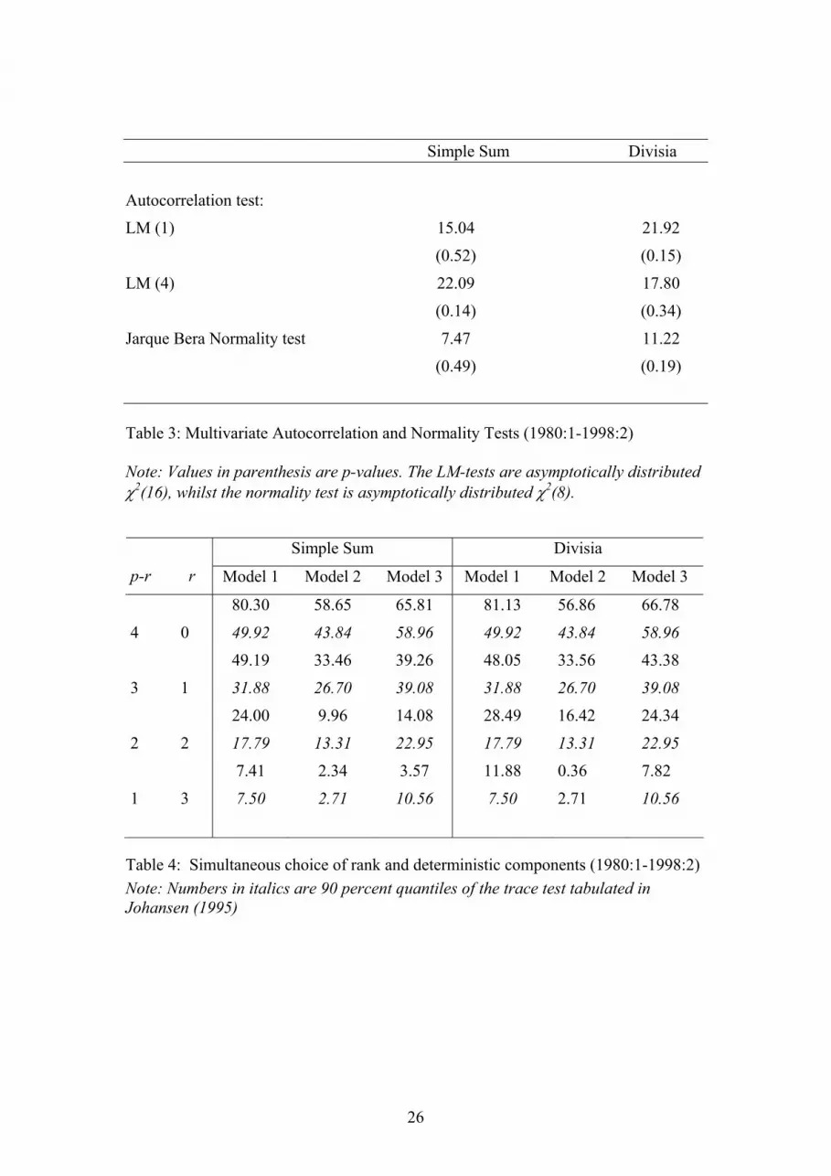
model of lag length k ttktktktt Dtzzzz εφδµ ++++Ψ+∆Γ++∆Γ=∆ −−−−− )1(111 L (3) whereµ is a constant and the error term, tε , is independently and normally distributed, 11 ,, −ΓΓ kL , Ψ and φ are coefficient matrices, D consists of dummy variables4 and t is a trend variable. If rank r=Ψ)( , where << r0 q, implies existence of rq× matrices α and β such that 'αβ=Ψ and tz'β is I(0) (Johansen and Juselius, 1990). r is the number of cointegrating relationships and each column of β is a cointegrating vector. In the current study, trace tests are used to determine the cointegration rank (see Johansen, 1995)5. The results, however, are sensitive to the choice of the lag length (k). Some model selection criteria could be used in determining the lag length but different criteria often suggest different orders. A more appropriate method is to combine this with misspecification tests by choosing the lag length to ensure that the underlying assumptions of the VAR model are satisfied (Johansen, 1995). More specifically, to check whether the residuals in the Johansen VAR are free from serial correlation, conditional heteroscedasticity and the distribution of the residuals is normal. Our experimentation uses a range of lags (VAR lag lengths of 1-8) and is based on the misspecifications tests. For a VAR of order 6, the LM and JB tests, represented in table 3, do not show any sign of misspecification nor do the univariate ARCH tests6.

[Table 3 about here] In testing for cointegration, the question of whether a constant and trend should enter the long run relationship also arises. There are in general 5 possible ways of incorporating these deterministic components into the analysis (see Johansen 1992, Hansen and Juselius, 1995) but generally the most and the least restrictive ones are excluded (see, for example, Drake (1996)). Therefore, the three models of interest to us have the following specification. The model that we refer to as model 1 is the most restrictive model. It does not allow for linear trends in the data. The only deterministic components in the model are the intercepts in the cointegration relations.

8

A less restrictive model is referred to as model 2. The model allows for linear trends in the data, but it is assumed that there are no trends in the cointegration relations. It also has a non-zero intercept. The model referred to as model 3 is the least restrictive. It also allows for a linear trend in the cointegration space.

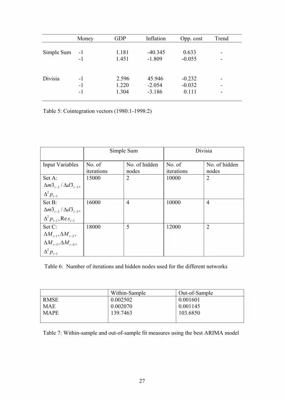
In order to determine which of the three possible deterministic specifications is the most appropriate in the cointegration, Johansen (1992) suggests applying the Pantula (1989) principle. In so doing, the rank order and the presence of the deterministic components are jointly determined. In practice this involves estimating all the 3 models outlined above and conducting the trace test to determine the cointegration rank sequentially from the most restrictive to the least restrictive specification. The first time the null hypothesis of r cointegrating vectors is not rejected indicates both the cointegration rank and the appropriate specification for the deterministic components. Results from the application of the Pantula (1989) principle, reported in table 4, suggest that model 2 should be used for the Simple Sum system and the rank is 2 whereas model 2 should be used and the rank is 3 for Divisia system. The cointegrating vectors for both systems are presented in table 5.

[Table 4 about here]

[Table 5 about here] 4.2.2 Short-run Equations for Inflation In this section we present estimation results for single error correction equations of inflation. For both Simple Sum and Divisia, the corresponding second cointegrating vector is used for specifying their short-run equations of the form (3) for inflation for the period 1981Q2 to 1998Q2. These cointegrating vectors have been chosen since the signs of the coefficients of their components are consistent with economic theory (see Doornik et al., 1998). Money affects prices with long lags, approximately two years (Drake et al., 2000) and hence 7 lags of each of the independent variables have been used.7 Following the general to specific methodology (Hendry, 1993), parameters insignificant at the 5% significance level were deleted and the equations rerun, using the ordinary least squares method, until just significant parameters remained. The error correction terms were kept in the equations at all the times and eliminated in the final stage if they were not significant. This strategy eventually resulted in the equations given by equations (4) and (5) for the Euro M3 and Euro Divisia M3 respectively. Here also the diagnostic tests do not show any signs of misspecification. Simple Sum

( ) ( ) ( )000026.0102.0054.0

Re000062.0533.03121.0 112

22

ttttt spmp ε++∆−∆=∆ −−− (4)

Res = is 2nd cointegrating vector for a VAR lag = 7


LM (1) = 0.38 (0.54) LM (4) = 1.61 (0.81) LM (8) = 8.61(0.38)

ARCH (1) = 1.70 (0.19) ARCH (4) = 1.61 (0.81) ARCH (8) = 2.22 (0.97)

9

Divisia

( ) ( ) ( )000027.0102.0054.0

Re000070.0537.03141.0 112

32

ttttt spdp ε++∆−∆=∆ −−− (5)

Res = is the 2nd cointegrating vector for a VAR lag = 7


LM (1) = 1.34 (0.25) LM (4) = 3.18 (0.53) LM (8) = 5.94(0.65)

ARCH (1) = 0.05 (0.83) ARCH (4) = 5.64 (0.23) ARCH (8) = 8.81 (0.36)

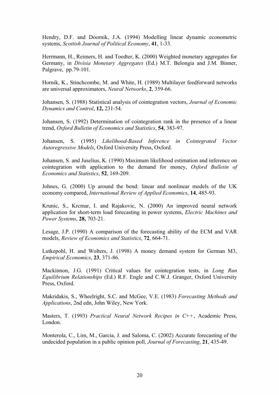
4.3 Nonlinear Models: Neural Networks Neural networks are composed of highly interconnected processing elements (nodes) that work simultaneously to solve specific problems. In time series analysis they are used as nonlinear function approximators. They take in a set of inputs and produce a set of outputs according to some mapping rules predetermined in their structure.

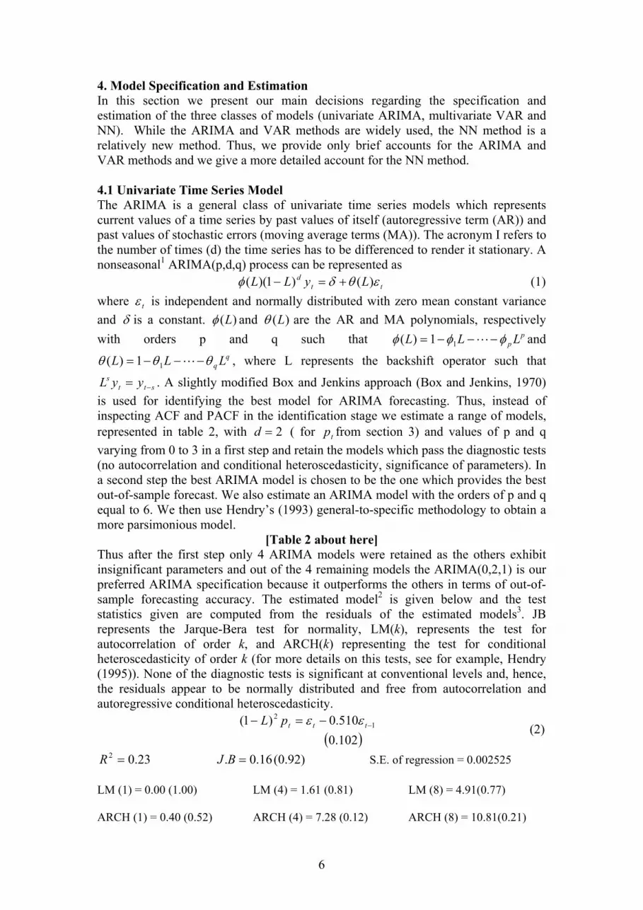
[Figure 2 about here] This paper considers the most popular form of NN called the feedforward network. Figure 2 depicts such a network that consists of layers of nodes. The input layer and output layer represent the input and output variables of the model. Between them lie one or more hidden layers that progressively transform the original input stimuli to final output and hold the networks ability to learn nonlinear relationships. For a feedforward NN with one hidden layer, the general prediction equation, given by Faraway and Chatfield (1998), for computing a forecast of ty using an input vector ( )mxxx ,,, 21 L may be written in the form ))((ˆ ∑∑ ++=

iiih

hchhocot xwwgwwfy (6)

where chw denote the weights for the connections between a constant input, usually taken as 1, and the hidden nodes and cow denotes the weight of the direct connection between the constant input and the output. The weights ihw and how denote the weights for the other connections between the input and hidden nodes and between hidden and the output nodes respectively. The two functions f and g denote the activation functions used in the hidden layer and the output layer respectively. NN have to be trained in order to be able to use them to perform certain tasks like predicting a response corresponding to a new input pattern. The training procedure involves iteratively modifying the randomly initialised weights of the NN to minimise

some kind of error function usually the mean square error (MSE), 2)ˆ(1tt yy

n−∑ .

Various standard optimisation techniques such as the conjugate gradient and quasi-Newton methods exist for minimising the error function, however, in application studies, the backpropagation algorithm (Rumelhart et al., 1986) developed by the

10

neural network community is the most popular training algorithm used. Standard optimisation techniques tend to converge faster than the backpropagation algorithm but this advantage is overshadowed by the fact that the latter is computationally more efficient (Monterola et al., 2002). Moreover, the backpropagation algorithm generally has better generalisation (performs well on unseen data) than standard optimisation techniques (Cubiles-de-la-Vega et al., 2002), hence is our preferred algorithm despite the greater time required for convergence. However, it is well known that the backpropagation algorithm used for training suffers from the local minimum problem. Randomly selecting initial weights for training is a common approach, however, if these initial weights are located close to local minima, the algorithm is likely to converge to a local minimum. Some researchers have tried to overcome this problem by, for example, using genetic algorithms (Shazly and Shazly, 1999) and simulated annealing (Masters, 1993). Even then there is no assurance that such measures will help the optimisation algorithm to converge to a global minimum. We follow the most commonly used method to find the best local minimum or even the global minimum, more specifically, we restart the training with different weights. The actual number of restarts employed in practice is generally limited by the computing time required to train a NN (Plasmans et al., 1998). In this work we therefore use 10 restarts. 4.3.1 Designing the Neural Networks Apart from the weights of the NN, there are many other parameters, like the number of input variables, the combination of input variables, the number of hidden layers and hidden nodes, the types of activation functions in the hidden and output layers, the value of the learning rate and the momentum rate and the amount of training which are also unknown. As we mentioned earlier there are no established rules to help us in choosing the appropriate values of these parameters and we have to resort to trial and error to obtain their appropriate values. Clearly, experimenting over the whole parameter space of the parameters is beyond the scope of the paper. In this study, therefore, we focus on experimenting with the different values of key parameters like initial weights, the number of hidden nodes, amount of training required, different sets of input variables and we draw attention to the other issues that need to be considered while making the choices for the remaining parameters of the NN. The common practice has been to construct NN using the same input variables as in VAR models to allow direct comparison between them. However, such a procedure is biased towards the linear model as the regressors from the linear equation tell us about linear correlation and this is not appropriate for nonlinear relationships modelled by the NN (Zhang et al., 1998). For these reasons, we feel justified to use the ‘best’ set of input variables for the NN. A modified version of the preferred model of the relationship between inflation and money of Binner et al., (2002) adapted originally from Dorsey (2000, pp.34) given by equation (7) below is used. However, for comparative purposes we also construct NN using the set of input variables of the VAR models and using the set of input variables of the VAR models from which the error correction term has been excluded. ),,,,( 1

24321

2−−−−− ∆∆∆∆∆=∆ tttttt pMMMMfp tε+ (7)

11

Hidden layers play a very important role for the successful applications of the NN as they allow NN to perform nonlinear mapping between the input and the output. Without hidden nodes, NN are equivalent to linear statistical model (see, for example, Warner and Misra (1996)). It has been shown that a 3 layer NN, i.e., a NN with only one hidden layer can approximate any function to any degree of accuracy (Hornik et al., 1989). Two hidden layer NN could be more beneficial to certain problems (Barron, 1994), however, given our relatively small sample and the fact that the number of parameters increases rapidly with each layer (Tkacz, 2001), we focus on 3 layer NN in the present study. The choice is more complicated for the number of hidden nodes. Usually few hidden nodes are preferred as there is less likelihood of overfitting, i.e. encountering problems of drawing too many characteristics from the data used for training, and a tendency to yield better generalisation. But NN with too few hidden nodes may not have enough power to model and learn the richness of the data (Church and Curram, 1996). Similar problems are encountered if the NN are not trained to the right degree. Inadequately training a NN will lead to missing patterns in the data while excessive training will result in overfitting. We use a grid search to jointly determine the appropriate number of hidden nodes and the amount of training required (Gorr et al., 1994). We consider 5 networks with hidden units between 1 and the number of input variables (Balkin and Ord, 2000) that is 5 in our case. Preliminary investigation over the number of training ranging from 10,000 to 50,000, suggested that better results are obtained in the range 15000 to 20000 for the Simple Sum NN models and in the range 10000 to 15000 for the Divisia model. Therefore, extensive experimentation is constrained to these ranges with increments of 1000. Since we perform 10 restarts for each point in our grid, this means that 300 NN for each set of input variables and monetary aggregate are investigated, i.e. a total of 1800 NN are run in this investigation. The logistic function )1/(1)( xexf −+= is the most popular activation function among researchers for the hidden layer. However, we use the hyperbolic tangent (tanh) function, )/()()( xxxx eeeexf −− +−= as it has been used very successfully in inflation forecasting experiments (see, for example, Binner et al., (2002)). It is also generally held that tanh gives rise to faster convergence of training algorithms than logistic functions (Bishop, 1995). For the output layer, we follow the recommendation of Rumelhart et al. (1995) who suggest the use of the linear function xxf =)( for time series prediction with continuous output. The remaining parameters for the NN, the learning and momentum rates for the backpropagation algorithm are set as the default values of Matlab 6.0, i.e. 0.01 and 0.9 respectively (see, for example, Bishop (1995), for more details on these parameters). In addition to the parameters of the NN, there are some other factors such as the data normalisation and performance measures that affect the performance of NN (Zhang et al., 1988). In practice NN training can be made more efficient by preprocessing the data as this enables the network to extract valuable information (Gately, 1996) and to significantly reduce the time necessary to complete training (Krunic et al., 2000). In this paper we use one of the most common forms of preprocessing which consists of rescaling the data in the range [-1, 1] so that they have similar values. This choice is motivated by the fact that the input variables used for NN modelling differ by several

12

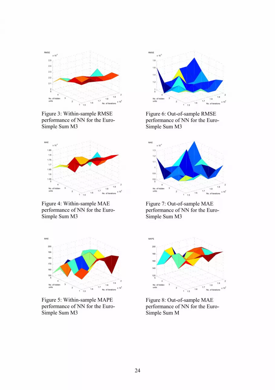
orders of magnitude and the sizes of variables do not necessarily reflect their relative importance in finding out the required outputs (Bishop, 1995). Another issue of concern is related to performance measures. There are several measures of accuracy but each of them has advantages and limitations (Makridakis et al., 1983). For this reason none of them is universally accepted as the best measure of accuracy and hence in this study we shall be making use of a number of performance measures. 5. Predictive Performance Assessment The NN should be tested on a validation set after they have been trained and the one leading to the minimum forecast error in the validation set should provide the best generalisation and is normally retained to evaluate its forecasting performance on a test sample. However, one of the main disadvantages of NN, as mentioned above, is that it requires an enormous amount of data, if the series are short or not representative of the process being modelled the NN might not perform well (Balkin and Ord, 2000). Thus in studies with small data sets it is common to use the test set for both validation and testing purposes (Zhang et al., 1998). That is the route followed in this paper given that the data set available to us is quite modest by the standards of NN analysis. Three traditional performance measures are first used to compare the fit and forecasting accuracy of alternative models: root mean square error (RMSE), mean absolute error (MAE), and mean absolute percentage error (MAPE). Before calculating these measures the NN forecasts are backtransformed to the same units as their actual values to make them comparable. Figures 3, 4 and 5 show the within-sample RMSE, MAE and MAPE performances respectively and figures 6, 7 and 8 show the corresponding out-of-sample performances of the Simple Sum NN constructed with the set of input variables as in equation 7. The patterns shown by the RMSE, MAE and MAPE, within-sample and out-of sample, for different number of hidden nodes and amount of training across different sets of input variables are in general similar. A comparison of the within-sample RMSE to that of the out-of-sample RMSE reveals that as the number of hidden nodes and amount of training are increased the within-sample forecast error decreases but, as expected, the reversed pattern is observed with the out-of-sample forecasts. This clearly demonstrates that with too many hidden nodes and excessive training, poor generalisation will occur and hence the need to appropriately choose these parameters. The MAE shows a similar pattern to that of the RMSE, however, the movement across both surfaces is not always in congruence. The discrepancies in the performance measures become more apparent as the RMSE and MAE are compared to the MAPE. The differences are apparently due to the inherent limitations in each of the performance measures. Therefore, these observations show that choosing the best model on the basis of just one performance measure would be misleading and thus in the current study the best model is chosen to be the one which consistently shows small forecast errors across each of the three performance measures and which also provides the best trade-offs between within-sample and out-of-sample forecast errors. On this basis, the number of iterations and hidden nodes chosen are reported in table 6 for each set of input variables (sets A, B and C also defined table in 6) for each monetary aggregate. One noticeable pattern in these values is that number of iterations or number of hidden nodes or both increase as the number of input variables increases. This could be due to the fact that the higher the

13

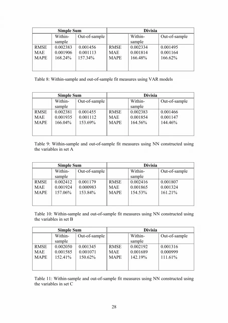
number of input variables, the higher the level of complexity of the NN and hence more hidden nodes or/and training are required to learn the relationship between input and output variables. The static forecasting performance of the ARIMA and VAR models are reported in tables 7 and 8 respectively, while those of the NN based on the three different sets of input variables are reported in tables 9, 10 and 11.

[Figures 3, 4, 5, 6, 7 and 8 about here] [Tables 6, 7, 8, 9, 10 and 11 about here]

A comparison of the results from the ARIMA and VAR forecasts suggest the multivariate models provide more accurate forecasts of Euro inflation. Looking at RMSE for example, the out-of-sample forecasting accuracy increases by about 9% with VAR models when compared to ARIMA models and hence the VAR models are retained as representatives for linear models for comparison with nonlinear NN. On comparing the results from VAR modelling and NN constructed with the same input variables (set B) as in the VAR models, it is not possible to discriminate between them as both of perform equally well in 12 comparisons of the within-sample and out-of-sample forecasts of the two monetary indices. NN constructed with the input variables from set A show a better performance but are still outperformed by the linear models in a few cases. However, a comparison of the results from the VAR modelling to those from NN constructed input variables are from set C, reveals that superior inflation forecasts are achieved using NN, both within-sample and out-of-sample, in every case examined. Looking again at the RMSE, for example, out-of-sample forecasting accuracy increases by approximately 10% with NN over VAR models. These results demonstrate the sensitivity of the NN to the choice of input variables and reveal that input variables used for building the linear models are not necessarily the most appropriate ones for the nonlinear models. We also evaluate the relative forecasting potential of the VAR and NN models by using a simple encompassing test (Fair and Shiller, 1990). Such a test has some advantages over the other performance measures (RMSE, MAE, MAPE) to compare the forecasts. Firstly, it can differentiate between competing forecasting models even if there are no big differences in the performance measures. Secondly, it helps to discriminate between models in cases where the performance measures are in favour of a particular model while despite having larger performance measures other competing models might contain vital information unique to them. Thirdly, such a test gives some statistical meaning to the forecasts of the NN relative to those of the linear models. The test is carried out by regressing the actual values of the changes in inflation on a constant, linear model forecasts )( Lf and NN forecasts )( Nf . If the t tests show that the coefficients of the forecasts of both models are significantly different from zero, then both models contain independent information that have power in forecasting the changes in inflation. If one of the coefficients of the forecasting models is significantly different from zero and the other one is not then the latter is just a subset of the former. In addition, the model with the significant coefficient contains further relevant information. Finally, if none of the coefficients are significantly different from zero then neither model is useful in forecasting the changes in inflation. The best NN forecasts obtained by using the input variables in C, are evaluated against the VAR forecasts. The results from the encompassing tests carried out for within-sample and out-of-sample forecasts are given below. The JB, LM and ARCH tests do not show any signs of misspecification. The results reveal that in every case only the coefficient of the NN forecast is significant at the

14

conventional 5% significance level which implies that that NN forecasts are statistically superior to the linear models forecasts and hence VAR forecasts are simply a subset of the NN. These results further confirm that better macroeconomic forecasts can be achieved with the use of nonlinear NN. Simple Sum Within-sample

( ) ( ) ( )232.0287.0000253.0

128.1165.00000007.02t

NLt ffp ε++−=∆

(8)


LM (1) = 2.47 (0.12) LM (4) = 5.35 (0.25) LM (8) = 12.30(0.14)

ARCH (1) = 0.26 (0.62) ARCH (4) = 0.63 (0.96) ARCH (8) = 3.80 (0.875)

Out-of-sample

( ) ( ) ( )689.0005.10006.0

349.10933.0000615.02t

NLt ffp ε++−−=∆

(9)


LM (1) = 0.25 (0.62) LM (4) = 3.60 (0.46)8

ARCH (1) = 1.46 (0.23) ARCH (4) = 5.82 (0.21)

Divisia Within-sample

( ) ( ) ( )323.0361.0000272.0

960.00647.000000268.02t

NLt ffp ε+++=∆

(10)


LM (1) = 3.80 (0.15) LM (4) = 3.83 (0.43) LM (8) = 10.39(0.24)

ARCH (1) = 0.14 (0.71) ARCH (4) = 3.69 (0.45) ARCH (8) = 7.87 (0.45)

15

Out-of-sample

( ) ( ) ( )830.0925.0000551.0

633.1969.0000411.02t

NLt ffp ε++−−=∆

(11)


LM (1) = 0.74 (0.39) LM (4) = 6.26 (0.18)

ARCH (1) = 0.47 (0.49) ARCH (4) = 5.93 (0.20)

Finally, on comparing the inflation forecasting performance of the two monetary indices firstly within a linear framework, it is found that Euro Divisia M3 has better within-sample convergence than its Simple Sum counterpart. However, the main property sought here is better generalisation, i.e. better out-of-sample performance that apparently Divisia fails to provide. When the impact of the two monetary indices on the prediction accuracy is evaluated in a nonlinear framework, overall the Simple Sum index has better within-sample convergence, however, the Divisia index clearly outperforms it in terms of out-of-sample convergence. These results do seem to suggest that one of the reasons for the poor historical performance of the Divisia index against the Simple Sum index could be attributed to incorrectly choosing linear models to evaluate the two monetary indices. These results corroborate the findings of Binner and Gazely (1999), Binner et al., (2002, 2003) and Gazely and Binner (1998, 2000) who have consistently found that the Divisia index outperforms its Simple Sum counterpart when evaluated using NN. 6. Summary and Conclusions There is growing evidence that macroeconomic series contain nonlinearities but linear models such as the ARIMA and VAR models are widely used for forecasting such series, despite the inability of linear models to cope with nonlinearities. In this paper we provide new empirical evidence on the relative macroeconomic forecasting performance of linear ARIMA and VAR models and the nonlinear NN. We also investigate whether the poor performance of the theoretically superior measure of monetary services, Divisia, relative to its Simple Sum counterpart could be attributed partly to the incorrect choice of linear models used to evaluate them. A considerable amount of research has been carried out in the recent years on NN. However, despite their ability to capture nonlinear relationships, findings generally do not allow any discrimination between conventional linear statistical techniques and NN. One of the main reasons for this is that there are no well defined guidelines to build NN for solving a particular task and their construction has involved a lot of subjectivity on the part of researchers, thereby considerably restricting the power of NN and ultimately leading to the results of many studies being dubious. In order to obtain the best possible NN forecasting model in this study, we have tried to keep the level of subjectivity to a minimum, particularly we perform rigorous experiments to determine the appropriate number of iterations, number of hidden nodes and the appropriate set of input variables. At the same time we have considered other issues like data processing, local minima problems and limitations of performance measures. Our best models for the NN outperform the traditionally used linear ARIMA and VAR models in macroeconomic forecasting and are statistically superior to them. The gain in forecasting accuracy in the NN is very likely to have emerged from the

16

capability of the NN to capture nonlinear relationships between macroeconomic variables. The first conclusion to be drawn from this result is that despite being constrained by the lack of large data samples in macroeconomics, NN can find be successfully applied in the field, provided extreme care is taken in designing the network. However, at this stage we would not recommend the policy makers, such as the ECB who require inflation forecasts, to abandon the use of conventional statistical techniques in favour of NN. The latter still has some very serious limitations, e.g., particularly time consuming trial and error procedures and the lack of available statistical techniques for analyzing the relationship between input and output variables. However, till such problems are overcome, we would strongly suggest that the ECB and macroeconomic forecasters use NN as a complementary tool for forecasting. Another recommendation to the ECB involves the use of monetary aggregates for their monetary policy strategy. It is widely accepted that the Simple Sum procedure is inappropriate and the weighted Divisia index is a superior measure of monetary services flow. However, the Divisia index does not always outperform its Simple Sum counterpart in empirical studies, explaining the reluctance of the ECB to use the weighted monetary aggregate instead of M3. The results of this study suggest that the poor performance of the Divisia index can be attributed to a certain extent to the incorrect choice of linear statistical methods used to evaluate its performance relative to the Simple Sum index, as the Divisia clearly outperforms the Simple Sum index when evaluated in a nonlinear framework but not in a linear framework. However, these results should only be considered as indicative as we have not performed an exhaustive experimentation to find the best Simple Sum and Divisia NN forecast models, as the overriding aim was to evaluate linear ARIMA and VAR models and nonlinear NN models. Nonetheless, on the basis of the results at hand, and based on similar results obtained by Binner and Gazely (1999), Binner et al., (2002, 2003) and Gazely and Binner (1998, 2000), it appears that Divisia consistently outperforms the Simple Sum index when evaluated in a nonlinear framework. Thus our recommendation to the ECB would be to at least pay more serious attention to the behaviour of the Divisia monetary aggregate. Finally, we end by providing a recommendation on how this work can be taken a step further. Although NN considered in this paper outperform traditional econometric models in forecasting Euro inflation, we believe that the forecasting accuracy of NN can still be improved. We performed a grid search to determine the optimum number of hidden nodes and training required and performed some experimentation to find the optimum set of input variables. However, ideally, a NN for a particular task has to be optimised over the entire parameter space of the learning rate, momentum rate, number of hidden layers and nodes, combination of input variables and activation functions. In that respect, NN combined with genetic algorithm optimization techniques (Nag and Mitra, 2002), can potentially be used for building more accurate models for forecasting Euro inflation and is recommended for future research.

Acknowledgments The authors gratefully acknowledge the help of Mr Livio Stracca (see Stracca (2001)) for making the Euro area data available and Professor David Edgerton from Lund University, Sweden for providing very helpful comments.

17

References Adya, M. and Calopy, F. (1998) How effective are neural networks at forecasting and prediction? A review and evaluation, Journal of Forecasting, 17, 481-95. Balkin, S.D. and Ord, J.K. (2000) Automatic neural network modeling for univariate time series, International Journal of Forecasting, 16, 509-15.

Barnett, W.A. (1980) Economic monetary aggregates: an application of the index numbers and aggregation theory, Journal of Econometrics, 14, 11-48. Reprinted in The Theory of Monetary Aggregation (Ed.) W.A. Barnett and A. Serletis, North Holland, Amsterdam, pp. 11-48.

Barnett, W.A. (1982) The optimal level of monetary aggregation, Journal of Money, Credit and Banking, 14, 687-710.

Barnett, W.A and Chen, P. (1986) Economic theory as a generator of measurable attractors. Mondes en Develppement 14: Reprinted in Laws of Nature and Human Conduct: Specificities and Unifying Themes (Ed.) I. Prigogine and M. Sanglier, G.O.R.D.E.S., Brussels, pp. 209-24.

Barnett, W.A. and Chen, P. (1988a) The aggregation-theoretic monetary aggregates are chaotic and have strange attractors: an econometric application of mathematical chaos, in Dynamic Econometric Modeling, Proceedings of the Third International Symposium on Economic and Econometrics (Ed.) W.A. Barnett and E.R. Berndt and H. White, Cambridge University Press, UK, pp 199-245.

Barnett, W.A. and Chen, P. (1988b) Deterministic chaos and fractal attractors as tools for nonparametric econometric inference, Dynamical Computer Modeling, 10, 275-96.

Barnett, W.A. and Hinich, M.J. (1992) Empirical chaotic dynamics in Economics. Annals of Operation Research, 37, 1-15.

Barnett, W.A. and Hinich, M.J. (1993) Has chaos been discovered with economic data?, in Evolutionary Dynamics and Nonlinear Economics (Ed.) P. Chen and R. Day, Oxford University Press, New York, pp. 254-63.

Barnett, W.A., Fisher, D. and Serletis, A. (1992) Consumer theory and the demand for money, Journal of Economic Literature, 30, 2086-119, reprinted in The Theory of Monetary Aggregation (Ed.) W.A. Barnett and A. Serletis, North Holland, Amsterdam, pp. 389-427.

Barron, A.R. (1994) A comment on “Neural networks: a review from a statistical perspective”, Statistical Science, 9, 33-5. Binner, J.M. and Gazely, A.M. (1999) A neural network approach to inflation forecasting: the case of Italy, Global Business and Economics Review, 1, 76-92.

18

Binner, J.M., Gazely, A.M. and Chen, S. (2002) Financial innovation and Divisia indices in Taiwan: a neural network approach, European Journal of Finance, 8, 238-47. Binner, J.M., Gazely, A.M., Chen S.H. and Chie, B.T. (2003) Financial innovation and Divisia money in Taiwan: comparative evidence from neural networks and vector error correction forecasting models, Contemporary Economic Policy (forthcoming). Bishop, C.M. (1995) Neural Networks for Pattern Recognition, Oxford University Press, New York. Box, G.P. and Genkins, G.M. (1970) Time series analysis and forecasting: the Box-Jenkins approach, Holden-day, San Francisco. Chen, P. (1988) Empirical and theoretical evidence of economic chaos, Systems Dynamic Review, 4, 81-108. Church, K.B. and Curram, S.P. (1996) Forecasting consumers’ expenditure: a comparison between econometric and neural network models, International Journal of Forecasting, 12, 255-67. Chrystal, K.A. and MacDonald, R. (1994) Empirical evidence on the recent behavior and usefulness of Simple Sum and weighted measures of money stock. Proceedings from Federal Reserve Bank of St. Louis, March/April.

Cubiles-de-la-Vega, M., Pino-Mejías, R., Pascual-Acosta, A. and Muñoz-García, J. (2002) Building neural network forecasting models from time series ARIMA models: a procedure and a comparative analysis, Intelligent Data Analysis, 6, 53-95.

De Brouwer, G. and Ericsson, N.R. (1998) Modeling inflation in Australia, Journal of Business and Economics, 16, 433- 49. DeCoster, G.P. and Mitchell, D.W. (1991) Nonlinear monetary dynamics, Journal of Business and Economics Statistics, 9, 455-61. Dickey, D.A. and Fuller, W.A. (1979) Distribution of the estimators for autoregressive time series with a unit root, Journal of the American Statistical Association, 74, 427-31. Doornik, J.A., Nielsen, B. and Hendry, D.F. (1998) Inference in cointegrating models: UK M1 revisited, Journal of Economic Surveys, 12, 533-72. Dorsey, R.E. (2000). Neural networks with Divisia money: better forecasts of future inflation?, in Divisia Monetary Aggregates: Theory and Practice (Ed.) M.T. Belongia and J.M. Binner, Palgrave, New York, pp. 28-43. Drake, L. (1996) Relative prices in the UK personal sector money demand function, Economic Journal, 106, 1209-26. Drake, L., Chrystal, K.A., Binner, J.M. (2000) Weighted monetary aggregates for the UK, in Divisia Monetary Aggregates: Theory and Practice (Ed.), M.T. Belongia, J.M. Binner, Palgrave, New York, pp. 47-78.

19

Drake, L., Mullineux, A.W. and Agung, J. (1997) One Divisia money for Europe. Applied Economics 29: 775-786. Drake, L. and Mills, T.C. (2002) Is M3 an appropriate aggregate for guiding ECB monetary policy, Loughborough University Working Paper. ECB. (1999a) The Stability-oriented monetary policy strategy of the Eurosytem. ECB monthly Bulletin. January, 39-50. ECB. (1999b) Euro area monetary aggregates and their role in the Eurosystem’s monetary policy strategy, ECB Monthly Bulletin, February, 29-46. ECB. (2000) The two pillars of the ECB’s monetary policy strategy, ECB Monthly Bulletin, November, 37-48. Fair, C.R. and Shiller, R. (1990) Comparing information in forecasts from econometric models, The American Economic Review, 80, 375-89. Faraway, J. and Chatfield, C. (1998) Time series forecasting with neural networks: a comparative study using airline data, Applied Statistics, 47, 231-50. Gately, E. (1996) Neural Networks for Financial Forecasting, John Wiley, New York. Gazely, A.M. and Binner J.M. (1998) Better forecasts of future inflation? The neural network approach, Internet Journal of Financial Information Systems, February. http://www.shu.ac.uk/schools/fsl/fisjnl//vol1996/pprs1997/fisc97.htm Gazely, A.M. and Binner, J.M. (2000) The application of neural networks to the Divisia index debate: evidence from three countries, Applied Economics, 32, 1607-15. Gorr, W.L. and Nagin, D. and Szcypula, J. (1994) Comparative study of artificial neural network and statistical models for predicting student grade point averages, International Journal of Forecasting, 10, 17-34.

Granger, C.W.J. (1981) Some properties of time series data and their use in econometric model specification, Journal of Econometrics, 16, 121-30.

Haggan, V. and Ozaki, T. (1981) Modeling nonlinear vibrations using an amplitude-dependent autoregressive time series model, Biometrika, 68, 189-96.

Hansen, H. and Juselius, K. (1995) Cats in Rats. Cointegration Analysis of Time Series, Estima, Evaston, IL, USA.

Hendry, D.F. (1993) Econometrics: Alchemy or Science? Blackwell Publishers: Oxford, UK. Hendry, D.F. (1995) Dynamic Econometrics. Oxford University Press, Oxford.

20

Hendry, D.F. and Doornik, J.A. (1994) Modelling linear dynamic econometric systems, Scottish Journal of Political Economy, 41, 1-33. Herrmann, H., Reimers, H. and Toedter, K. (2000) Weighted monetary aggregates for Germany, in Divisia Monetary Aggregates (Ed.) M.T. Belongia and J.M. Binner, Palgrave, pp.79-101. Hornik, K., Stinchcombe, M. and White, H. (1989) Multilayer feedforward networks are universal approximators, Neural Networks, 2, 359-66.

Johansen, S. (1988) Statistical analysis of cointegration vectors, Journal of Economic Dynamics and Control, 12, 231-54.

Johansen, S. (1992) Determination of cointegration rank in the presence of a linear trend, Oxford Bulletin of Economics and Statistics, 54, 383-97.

Johansen, S. (1995) Likelihood-Based Inference in Cointegrated Vector Autoregressive Models, Oxford University Press, Oxford. Johansen, S. and Juselius, K. (1990) Maximum likelihood estimation and inference on cointegration with application to the demand for money, Oxford Bulletin of Economics and Statistics, 52, 169-209. Johnes, G. (2000) Up around the bend: linear and nonlinear models of the UK economy compared, International Review of Applied Economics, 14, 485-93. Krunic, S., Krcmar, I. and Rajakovic, N. (2000) An improved neural network application for short-term load forecasting in power systems, Electric Machines and Power Systems, 28, 703-21. Lesage, J.P. (1990) A comparison of the forecasting ability of the ECM and VAR models, Review of Economics and Statistics, 72, 664-71. Lutkepohl, H. and Wolters, J. (1998) A money demand system for German M3, Empirical Economics, 23, 371-86. Mackinnon, J.G. (1991) Critical values for cointegration tests, in Long Run Equilibrium Relationships (Ed.) R.F. Engle and C.W.J. Granger, Oxford University Press, Oxford. Makridakis, S., Wheelright, S.C. and McGee, V.E. (1983) Forecasting Methods and Applications, 2nd edn, John Wiley, New York. Masters, T. (1993) Practical Neural Network Recipes in C++, Academic Press, London.

Monterola, C., Lim, M., Garcia, J. and Saloma, C. (2002) Accurate forecasting of the undecided population in a public opinion poll, Journal of Forecasting, 21, 435-49.

21

Moshiri, S. and Cameron, N. (2000) Neural networks versus econometric models in inflation forecasting, Journal of Forecasting, 19, 201-17. Nag, A.K. and Mitra, A. (2002) Forecasting daily foreign exchange rates using genetically optimized neural networks, Journal of Forecasting, 21, 501-11. Pantula, G. (1989) Testing for unit roots in the time series data, Econometric Theory 5, 256-71. Plasmans, J., Verkooijen, W. and Daniels, H. (1998) Estimating structural exchange rate models by artificial neural networks, Applied Financial Economics, 8, 541-51. Rumelhart, D.E., Durbin, R., Golden, R. and Chauvin, Y. (1995) Backpropagation: the basic theory, in Backpropagation: Theory, Architectures, and Applications (Ed.) Y. Chauvin and D.E. Rumelhart, Lawrence Erlbraum Associates, New Jersey. Rumelhart, D.E., Hinton, G.E. and Williams, R.J. (1986) Learning internal representations by error propagation, in Parallel Distributed Processing: Exploration in the Microstructure of Cognition, Vol 1 (Ed.) D.E. Rumelhart and J.L. McClelland, MIT Press, Cambridge MA.

Shazly, M.R.E. and Shazly, H.E.E. (1999) Forecasting currency prices using genetically evolved neural network architecture, International Review of Financial Analysis, 8, 67-82.

Shoesmith, G.L. (1992) Cointegration, error correction and improved regional VAR forecasting, Journal of Forecasting, 11, 91-109.

Shoesmith, G.L. (1995) Long term forecasting of noncointegrated and cointegrated regional and national models, Journal of Regional Science, 35, 43-64.

Stanca, L. (1999) Asymmetries and nonlinearities in Italian macroeconomic fluctuations, Applied Economics, 31, 483-99. Stock, J.H. and Watson, M.W. Forecasting inflation, Journal of monetary Economics, 44, 293-335. Stracca, L. (2001) Does liquidity matter?: Properties of a synthetic Divisia monetary aggregate in the Euro area, Working Paper Series 79, European Central Bank. Tiao, G.C. and Tsay, R.S. (1994) Some advances in non-linear and adaptive modelling in time-series, Journal of Forecasting, 13, 109-31. Tkacz, G. (2001) Neural network forecasting of Canadian GDP growth, International Journal of Forecasting, 17, 57-69. Tong, H. (1990) Nonlinear Time Series. A Dynamical System Approach. Oxford University Press, Oxford, UK.

22

Warner, B. and Mishra, M. (1996). Understanding neural networks as statistical tools, The American Statistician, 50, 284-93. Zhang, G., Patuwo, B.E. and Hu, Y.H. (1998) Forecasting with artificial neural networks: the state of the art, International Journal of Forecasting, 14, 17-34.

Figure Captions 1. Simple Sum M3 index versus Divisia M3 index 2. NN model 3. Within-sample RMSE performance of NN for the Euro-Simple Sum M3 4. Within-sample MAE performance of NN for the Euro-Simple Sum M3 5. Within-sample MAPE performance of NN for the Euro-Simple Sum M3 6. Out-of-sample RMSE performance of NN for the Euro-Simple Sum M3 7. Out-of-sample MAE performance of NN for the Euro-Simple Sum M3 8. Out-of-sample MAE performance of NN for the Euro-Simple Sum M3

Table Captions

1. ADF unit root tests (1980:1-1998:2) 2. ARIMA models considered. Y represents Yes and N represents N 3. Multivariate Autocorrelation and Normality Tests (1980:1-1998:2) 4. Simultaneous choice of rank and deterministic components (1980:1-1998:2) 5. Cointegration vectors (1980:1-1998:2) 6. Number of iterations and hidden nodes used for the different networks 7. Within-sample and out-of-sample fit measures using the best ARIMA model 8. Within-sample and out-of-sample fit measures using VAR models 9. Within-sample and out-of-sample fit measures using NN constructed using the

variables in set A 10. Within-sample and out-of-sample fit measures using NN constructed using the

variables in set B 11. Within-sample and out-of-sample fit measures using NN constructed using the

variables in set C

23

Figures

0.7

0.8

0.9

1.0

1.1

1.2

1.3

1.4

1.5

80 82 84 86 88 90 92 94 96 98 00

Simple Sum index Divisia index

Figure 1: Simple Sum M3 index versus Divisia M3 index

Input Layer Hidden Layer Output Layer Figure 2: NN model

1

24

1.51.6

1.71.8

1.92

x 104

12

34

52

2.1

2.2

2.3

2.4

2.5

x 10-3RMSE

No. of hiddenunits

No. of iterations

Figure 3: Within-sample RMSE performance of NN for the Euro-Simple Sum M3

1.51.6

1.71.8

1.92

x 104

12

3

45

1.55

1.6

1.65

1.7

1.75

1.8

1.85

x 10-3MAE

No. of hiddenunits

No. of iterations

Figure 4: Within-sample MAE performance of NN for the Euro-Simple Sum M3

1.51.6

1.71.8

1.92

x 104

12

3

45

150

160

170

180

190

200

MAE

No. of hiddenunits

No. of iterations

Figure 5: Within-sample MAPE performance of NN for the Euro-Simple Sum M3

1.51.6

1.71.8

1.92

x 104

12

3

451

1.2

1.4

1.6

1.8

x 10-3RMSE

No. of hiddenunits

No. of iterations

Figure 6: Out-of-sample RMSE performance of NN for the Euro-Simple Sum M3

1.51.6

1.71.8

1.92

x 104

12

3

45

0.8

0.9

1

1.1

1.2

1.3

x 10-3MAE

No. of hiddenunits

No. of iterations

Figure 7: Out-of-sample MAE performance of NN for the Euro-Simple Sum M3

1.51.6

1.71.8

1.92

x 104

12

3

45

120

140

160

180

200

MAPE

No. of hiddenunits

No. of iterations

Figure 8: Out-of-sample MAE performance of NN for the Euro-Simple Sum M

25

Tables

Variable ADF Test Statistics Specification

3m -1.503 [T, 1] tm3∆ -4.834** [C, 0]

td3 -2.288 [T, 1]

td∆ -5.151** [C, 0]

ty -2.280 [T, 4]

ty∆ -6.932** [C, 0]

tp -2.451 [T, 2]

tp∆ -2.785 [T, 1]

tp2∆ -14.316 [C, 0]

tdualsm3 -3.825* [T, 1]

tdualsm3∆ -5.680** [C, 1]

tdualdm3 -3.781* [T, 1]

tdualdm3∆ -5.760** [C, 1] Table 1: ADF unit root tests (1980:1-1998:2) Notes: T: constant and trend, C: represents constant [, n], n: the number of lags used **: significant at 1%, *: significant at 5% Critical values are from MacKinnon (1991)

Models Retained

ARIMA(0,2,1) ARIMA(0,2,2) ARIMA(0,2,3) ARIMA(1,2,0) ARIMA(1,2,1) ARIMA(1,2,2) ARIMA(1,2,3) ARIMA(2,2,0) ARIMA(2,2,1) ARIMA(2,2,2) ARIMA(2,2,3) ARIMA(3,2,0) ARIMA(3,2,1) ARIMA(3,2,2) ARIMA(3,2,3) ARIMA(6,2,6)

Y N N Y N Y N N N N N N N N N Y

Table 2: ARIMA models considered. Y represents Yes and N represents N.

26

Simple Sum Divisia

Autocorrelation test:

LM (1)

LM (4)

15.04

(0.52)

22.09

(0.14)

21.92

(0.15)

17.80

(0.34)

Jarque Bera Normality test 7.47

(0.49)

11.22

(0.19)

Table 3: Multivariate Autocorrelation and Normality Tests (1980:1-1998:2) Note: Values in parenthesis are p-values. The LM-tests are asymptotically distributed χ2(16), whilst the normality test is asymptotically distributed χ2(8).

Simple Sum Divisia

p-r r Model 1 Model 2 Model 3 Model 1 Model 2 Model 3

4 0

80.30

49.92

58.65

43.84

65.81

58.96

81.13

49.92

56.86

43.84

66.78

58.96

3 1

49.19

31.88

33.46

26.70

39.26

39.08

48.05

31.88

33.56

26.70

43.38

39.08

2 2

24.00

17.79

9.96

13.31

14.08

22.95

28.49

17.79

16.42

13.31

24.34

22.95

1 3

7.41

7.50

2.34

2.71

3.57

10.56

11.88

7.50

0.36

2.71

7.82

10.56

Table 4: Simultaneous choice of rank and deterministic components (1980:1-1998:2) Note: Numbers in italics are 90 percent quantiles of the trace test tabulated in Johansen (1995)

27

Money GDP Inflation Opp. cost Trend Simple Sum -1 1.181 -40.345 0.633 - -1 1.451 -1.809 -0.055 - Divisia -1 2.596 45.946 -0.232 - -1 1.220 -2.054 -0.032 - -1 1.304 -3.186 0.111 - Table 5: Cointegration vectors (1980:1-1998:2)

Simple Sum Divisia

Input Variables No. of

iterations No. of hidden nodes

No. of iterations

No. of hidden nodes

Set A: ,3/3 32 −− ∆∆ tt dm

12

−∆ tp

15000 2 10000 2

Set B: ,3/3 32 −− ∆∆ tt dm

12

−∆ tp , 1Re −ts

16000 4 10000 4

Set C: 21 , −− ∆∆ tt MM ,

43 , −− ∆∆ tt MM ,

12

−∆ tp

18000 5 12000 2

Table 6: Number of iterations and hidden nodes used for the different networks Within-Sample Out-of-Sample RMSE MAE MAPE

0.002502 0.002070 139.7463

0.001601 0.001145 103.6850

Table 7: Within-sample and out-of-sample fit measures using the best ARIMA model

28

Table 8: Within-sample and out-of-sample fit measures using VAR models

Table 9: Within-sample and out-of-sample fit measures using NN constructed using the variables in set A

Table 10: Within-sample and out-of-sample fit measures using NN constructed using the variables in set B

Table 11: Within-sample and out-of-sample fit measures using NN constructed using the variables in set C

Simple Sum Divisia Within-

sample Out-of-sample Within-

sample Out-of-sample

RMSE MAE MAPE

0.002383 0.001906 168.24%

0.001456 0.001113 157.34%

RMSE MAE MAPE

0.002334 0.001814 166.48%

0.001495 0.001164 166.62%




RMSE MAE MAPE

0.002381 0.001935 166.04%

0.001455 0.001112 153.69%

RMSE MAE MAPE

0.002383 0.001854 164.56%

0.001466 0.001147 144.46%




RMSE MAE MAPE

0.002412 0.001924 157.06%

0.001179 0.000983 153.84%

RMSE MAE MAPE

0.002416 0.001865 154.53%

0.001807 0.001324 161.21%




RMSE MAE MAPE

0.002050 0.001585 152.41%

0.001345 0.001071 150.62%

RMSE MAE MAPE

0.002192 0.001689 142.19%

0.001316 0.000999 111.61%

29

Footnotes: 1 The reason for using nonseasonal ARIMA models is that the data provided to us had already been seasonally adjusted. 2 Values in parentheses under the estimated coefficients are standard errors 3 The numbers in parentheses behind the values of the test statistics are the corresponding p-values 4 The dummy variables are constructed to take into account the high peaks in the first differences in the measures of money in 1990Q3 and in the opportunity cost variables in 1994Q2. 5 The values of the trace statistics are found using CATS and RATS software. 6 The univariate ARCH test statistics are available from the authors upon request 7 The computations reported in this section were carried out on Eviews 4.0 8 Due to our short out-of-sample data set, misspecification tests could not be carried out for order 8

Vector autoregressive models versus neural networks in forecasting: an application to Euro-inflation...

Documents

Transcript of Vector autoregressive models versus neural networks in forecasting: an application to Euro-inflation...