Variational Bayesian Image Restoration With a Product of Spatially Weighted Total Variation Image...

IEEE TRANSACTIONS ON IMAGE PROCESSING, VOL. 19, NO. 2, FEBRUARY 2010 351

Variational Bayesian Image RestorationWith a Product of Spatially Weighted

Total Variation Image PriorsGiannis Chantas, Nikolaos P. Galatsanos, Senior Member, IEEE, Rafael Molina, and

Aggelos K. Katsaggelos, Fellow, IEEE

Abstract—In this paper, a new image prior is introduced andused in image restoration. This prior is based on products ofspatially weighted total variations (TV). These spatial weightsprovide this prior with the flexibility to better capture local imagefeatures than previous TV based priors. Bayesian inference isused for image restoration with this prior via the variationalapproximation. The proposed restoration algorithm is fully au-tomatic in the sense that all necessary parameters are estimatedfrom the data and is faster than previous similar algorithms.Numerical experiments are shown which demonstrate that imagerestoration based on this prior compares favorably with previousstate-of-the-art restoration algorithms.

I. INTRODUCTION

I MAGE restoration is a mature image processing topic withan over 30-year-long history. This problem is well known

to be ill posed, and, consequently, it requires regularization [1].The field of image restoration is very broad. Thus, an attempt

to survey it and do justice to all its contributors is outside thescope of this paper. Therefore, in what follows we referenceonly image restoration methods directly related to the proposedwork.

Total variation (TV) is a powerful concept for robust estima-tion [2]. It was first introduced as a regularizer for image restora-tion in [5]. Since then it has been used extensively and withgreat success for inverse problems because TV has the abilityto smooth noise in flat areas of the image and at the same timepreserve edges. For certain recent developments on TV basedimage recovery the interested reader is referred to [4] and [3].

Nevertheless, TV-based image restoration has certain short-comings. One of them is the selection of the regularization pa-

Manuscript received April 14, 2009; revised September 02, 2009. First pub-lished September 29, 2009; current version published January 15, 2010. Thiswork was supported in part by the research project (PENED), which was sup-ported in part by the E.U.-European Social Fund (75%) and the Greek Min-istry of Development-GSRT (25%), the “Comisión Nacional de Ciencia y Tec-nología” under contract TIC2007-65533, the Spanish research programme Con-solider Ingenio 2010: MIPRCV (CSD2007-00018), and the Greek-Spanish col-laboration program of Greek Ministry of Development-GSRT. The associateeditor coordinating the review of this manuscript and approving it for publica-tion was Prof. Eric Kolaczyk.

G. Chantas is with the Department of Computer Science, University of Ioan-nina, Greece, 45110 (e-mail [email protected]).

N. P. Galatsanos is with the Department of Electrical Engineering, Universityof Patras Rio, Greece 26500 (e-mail: [email protected]).

R. Molina is with the Departamento de Ciencias de la Computación e I. A.,Universidad de Granada, 18071 Granada, Spain (e-mail: [email protected]).

A. K. Katsaggelos is with the Department of Electrical Engineering and Com-puter Science, Northwestern University, Evanston, IL 60208-3118 USA (e-mail:[email protected]).

Digital Object Identifier 10.1109/TIP.2009.2033398

rameter which to a large extent until recently has been ad-hoc.Rudin et al. [5] consider the minimization of the TV energyfunction constrained by the sum of the square of the observa-tion errors being equal to , where represents an esti-mate of the noise variance, and is the number of observations,and then proceed to estimate both the image and the associatedLagrange multiplier to this constrained optimization problem.Bertalmio et al. [24] make the Lagrange multiplier region de-pendent. Bioucas-Dias et al. [12], using their majorization-min-imization approach [13], propose a Bayesian method to esti-mate the original image and regularization parameter assumingthat an estimate of the noise variance is available. Recently, aBayesian inference framework which requires the approxima-tion of the prior partition function and is based on the variationalapproximation was proposed to handle the simultaneous param-eter and image estimation [14].

An alternative image model has recently been proposed basedon the combination of several image priors [11], [23], and [16].It combines in product form multiple probabilistic models. Eachindividual model gives high probability to data vectors that sat-isfy just one constraint. Vectors that satisfy only this constraintbut violate others are ruled out by their low probability under theother terms of the product model. Such priors were learned in[11] and [23] using a large training set of images and stochasticsampling methods, in contrast to the approach proposed in [16]where the product prior is learnt only from the observations.Each term in the product defining the prior in [16] correspondsto the output of a high-pass linear filter and is Student’s-t dis-tributed. The main contribution of [16] is the introduction of aBayesian inference methodology based on the constrained vari-ational approximation that bypasses the difficulty of evaluatingthe normalization constant of product type priors.

Variational based Bayesian inference using TV and Stu-dent’s-t priors for the image has been used with success forblind image deconvolution (BID) problems also. In [17] aTV prior was used for the image while Gaussian priors wereused for the point spread function (PSF). In [18], a Student’s-tprior in product form was used for the image. However, thenormalization constant for this prior was approximated. Alsoin [18], a kernel based sparse Student’s-t prior was used forthe PSF. This prior provides a mechanism, for the first time, toestimate the spatial support of the PSF also.

In this paper, we contribute to the field of prior image mod-eling by combining the advantages of TV image modeling in[14] and Student’s-t Product of Experts (PoE) image modelingin [16]. The new image model has a number of novel features.

1057-7149/$26.00 © 2010 IEEE

352 IEEE TRANSACTIONS ON IMAGE PROCESSING, VOL. 19, NO. 2, FEBRUARY 2010

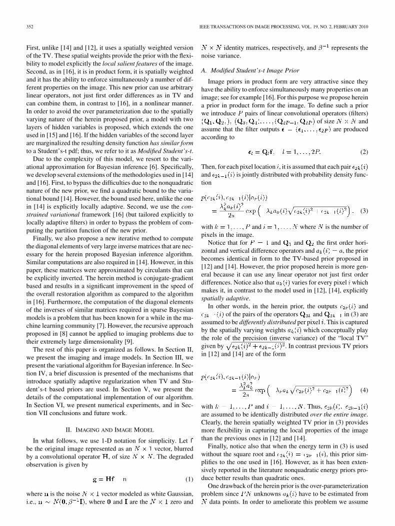
First, unlike [14] and [12], it uses a spatially weighted versionof the TV. These spatial weights provide the prior with the flexi-bility to model explicitly the local salient features of the image.Second, as in [16], it is in product form, it is spatially weightedand it has the ability to enforce simultaneously a number of dif-ferent properties on the image. This new prior can use arbitrarylinear operators, not just first order differences as in TV andcan combine them, in contrast to [16], in a nonlinear manner.In order to avoid the over parameterization due to the spatiallyvarying nature of the herein proposed prior, a model with twolayers of hidden variables is proposed, which extends the oneused in [15] and [16]. If the hidden variables of the second layerare marginalized the resulting density function has similar formto a Student’s-t pdf; thus, we refer to it as Modified Student’s-t.

Due to the complexity of this model, we resort to the vari-ational approximation for Bayesian inference [6]. Specifically,we develop several extensions of the methodologies used in [14]and [16]. First, to bypass the difficulties due to the nonquadraticnature of the new prior, we find a quadratic bound to the varia-tional bound [14]. However, the bound used here, unlike the onein [14] is explicitly locally adaptive. Second, we use the con-strained variational framework [16] (but tailored explicitly tolocally adaptive filters) in order to bypass the problem of com-puting the partition function of the new prior.

Finally, we also propose a new iterative method to computethe diagonal elements of very large inverse matrices that are nec-essary for the herein proposed Bayesian inference algorithm.Similar computations are also required in [14]. However, in thispaper, these matrices were approximated by circulants that canbe explicitly inverted. The herein method is conjugate-gradientbased and results in a significant improvement in the speed ofthe overall restoration algorithm as compared to the algorithmin [16]. Furthermore, the computation of the diagonal elementsof the inverses of similar matrices required in sparse Bayesianmodels is a problem that has been known for a while in the ma-chine learning community [7]. However, the recursive approachproposed in [8] cannot be applied to imaging problems due totheir extremely large dimensionality [9].

The rest of this paper is organized as follows. In Section II,we present the imaging and image models. In Section III, wepresent the variational algorithm for Bayesian inference. In Sec-tion IV, a brief discussion is presented of the mechanisms thatintroduce spatially adaptive regularization when TV and Stu-dent’s-t based priors are used. In Section V, we present thedetails of the computational implementation of our algorithm.In Section VI, we present numerical experiments, and in Sec-tion VII conclusions and future work.

II. IMAGING AND IMAGE MODEL

In what follows, we use 1-D notation for simplicity. Letbe the original image represented as an vector, blurredby a convolutional operator , of size . The degradedobservation is given by

(1)

where is the noise vector modeled as white Gaussian,i.e., , where and are the zero and

identity matrices, respectively, and represents thenoise variance.

A. Modified Student’s-t Image Prior

Image priors in product form are very attractive since theyhave the ability to enforce simultaneously many properties on animage; see for example [16]. For this purpose we propose hereina prior in product form for the image. To define such a priorwe introduce pairs of linear convolutional operators (filters)

of size andassume that the filter outputs are producedaccording to

(2)

Then, for each pixel location , it is assumed that each pairand is jointly distributed with probability density func-tion

(3)

with and where is the number ofpixels in the image.

Notice that for and and the first order hori-zontal and vertical difference operators and , the priorbecomes identical in form to the TV-based prior proposed in[12] and [14]. However, the prior proposed herein is more gen-eral because it can use any linear operator not just first orderdifferences. Notice also that varies for every pixel whichmakes it, in contrast to the model used in [12], [14], explicitlyspatially adaptive.

In other words, in the herein prior, the outputs andof the pairs of the operators and in (3) are

assumed to be differently distributed per pixel . This is capturedby the spatially varying weights which conceptually playthe role of the precision (inverse variance) of the “local TV”given by . In contrast previous TV priorsin [12] and [14] are of the form

(4)

with and . Thus,are assumed to be identically distributed over the entire image.Clearly, the herein spatially weighted TV prior in (3) providesmore flexibility in capturing the local properties of the imagethan the previous ones in [12] and [14].

Finally, notice also that when the energy term in (3) is usedwithout the square root and , this prior sim-plifies to the one used in [16]. However, as it has been exten-sively reported in the literature nonquadratic energy priors pro-duce better results than quadratic ones.

One drawback of the herein prior is the over-parameterizationproblem since unknowns have to be estimated from

data points. In order to ameliorate this problem we assume

CHANTAS et al.: VARIATIONAL BAYESIAN IMAGE RESTORATION 353

that each is a Gamma distributed hidden random variable[15], [16] according to

(5)Note that this distribution on is flexible enough to pro-

vide a range of restrictions on : from very vague informa-tion, which would be modeled when , to very precise in-formation which is obtained when . Note also that fromthe definition in (5), for a given , all the coefficients comefrom the same distribution with variance moving from infinityto zero, as changes from zero to infinity.

The marginal distribution of and can be com-puted in closed form and is given by

(6)

for and .This density function is very similar in form to the Student’s-t

pdf which is given by [6]

(7)

thus, in the rest of this paper we label it as Modified Student’s-t.It is important to note that this prior combines the advantagesof both TV-based and Student’s-t based priors. The formerbeing the ability to suppress noise and maintain edges in animage beyond the capabilities of linear filters [12], [14] and thelatter being the ability to explicitly introduce spatial adaptivitythrough the hidden random variables , which improvesthe prior modeling used in [15] and [16].

At this point, we note that we have not provided a prior forthe image, . This was intentional, because we cannot com-pute it in closed form. More specifically, it is difficult to definea prior for the image based on the prior in (3) because wecannot compute the partition function for such prior. First, thenonquadratic exponent in the pdf in (3) makes this calculationintractable even if our prior was not in product form .Furthermore, if we want to use a prior in product formeven with a quadratic exponent it is not possible to compute thepartition function [16]. Consequently, in the next section we by-pass the calculation of the partition function when the prior isdefined on by working in the domain of the filter outputs [16],where the prior in (3) can be used directly and there is no need todefine a prior for . The downside of this choice is that it is notobvious how to merge the estimates of all the ,to generate one estimate for . To handle this problem we willpropose the use of the constrained variational approach in thenext section.

In order to define the observation model in terms of, let us examine in some detail the prior model we

are using. Let us consider the image model in (3). If we re-move one component from it, for instance , we have aLaplace distribution with parameter . Since we considerjointly and , its partition function is proportionalto . Consequently, given we have two possibleexplanations for the data, one associated with and the otherwith .

We thus introduce an alternative observation model, whichis derived by applying the operators to the original imagingmodel in (1). This yields

(8)

where , , and, thus, .We finally arrive at the Bayesian modeling of our problem,

that is

(9)

where , , with, , with

, and, with the above proba-

bility distributions defined

(10)

(11)

and

(12)

This Bayesian model will be used for inference in the nextsection where we treat and as hidden variables and as aparameter vector to be estimated. Observe that we use the nota-tion to denote that is a set of hyperparameters which arenot treated as random variables. We could also have used .Notice also that we assume that the noise precision parameteris assumed to have been previously estimated.

III. VARIATIONAL INFERENCE WITH THE MODIFIED

STUDENT’S-T PRIOR

According to Bayesian inference we have to find the posteriordistributions for the hidden variables and given and theparameter vector . However, the marginal of the observationswhich is required to find the posteriors of the hidden variablesis hard to compute [6]. More specifically, the integral

(13)

is intractable.The variational algorithm that we describe in what follows,

bypasses this difficulty and maximizes a lower bound that


can be found instead of the log-likelihood of the observations[6], [10]. This bound is obtained by subtracting fromthe Kullback-Leibler divergence, which is always

positive, between an arbitrary and , that is

(14)

and is equal to

(15)

When , this bound is maximizedand . Because the exact posterior

cannot be found we use anapproximation of the posterior. The mean-field approximationis a commonly used approach to maximize the variationalbound w.r.t. [6], [10]. According to this approachthe hidden variables are assumed to be independent, i.e.,

. However, for the herein model this isstill not sufficient to obtain a closed form for which isnecessary for inference using this approach. More specifically,the square root in the joint which originates fromthe prior makes the definition of intractable.

A. Lower Bound for

For this purpose, we also introduce a lower bound on [14].More specifically, we use the inequality

(16)

which holds for and . Notice that equality holdswhen . This inequality is used at every pixel by setting

, for , whereare auxiliary variables used for this approximation. Using thisand the prior in (3), we have

(17)where [see (18), shown at the bottom of the page], for

.We also define and

. Let us now define

(19)

where

(20)

Then, since we have

(21)

and, consequently, the bound becomes tight when

(22)

Notice that the new lower bound is quadratic in the hiddenvariables ; thus, it is possible to find that maximizes it. Incontrast, the original bound was not quadratic in .

B. Constrained Variational Inference Algorithm

As we have already explained, , are used in-stead of to avoid the computation of the normalization constantof the prior on . Thus, a question that needs to be addressed ishow one finds given the different .

Unconstrained maximization of the boundresults in , where

,

, with ,, and

, where denotes theexpectation w.r.t the distribution of .

Clearly, each suggests a different estimate for given by. Thus, one needs to find a methodology to merge

the information from all into one estimate of .For this purpose, the constrained variational approximation

first proposed in [16] is applied. According to this approach,each is constrained to have the form

(23)

where is a vector, taken as the mean of the image, andthe image covariance matrix. This form is consistent withthe equation for whichand

with . Using this approx-imation, the parameters and are learned instead ofaccording to the herein constrained variational methodology.

We now present the maximization method by giving the up-dates for the variables of the bound in the th iteration. In theVE-step, the maximization of is performed

(18)


with respect to , and keeping and fixed, whilein the VM-step, the maximization of is per-formed with respect to and keeping , , and fixed.We have:

none VE-step

(24)none VM-step

(25)

The updates for the VE-Step are derived in the Appendix . Theseare

(26)

where [see (27) and (28), shown at the bottom of the page].From the above equations, it is clear that merges informa-

tion from all filters and is used as the estimate of .Finally, the approximate posterior of in the VE-step is

given by the equation shown at the bottom of the page, forand . Thus, the expectation of

w.r.t is

(29)

In the VM-step, the bound is maximized w.r.t to the parame-ters. To find we have to solve

(30)

where represents the expectation w.r.t. , which pro-duces

(31)

for and , where

(32)

For , we have

(33)

when this function is considered to be as a function of only.Thus, the update formula is

(34)

Similarly, for , we have

(35)

when this function is considered as a function of only. Thenis the root of the function which is proportional to the

derivative of with respect to

(36)

where is the digamma function. We find numeri-cally using the bisection method.

IV. SPATIAL ADAPTIVITY WITH TV AND

STUDENT’S-T BASED PRIORS

At this point, it is worth commenting on the spatialadaptivity properties of the restoration filter provided by the

(27)

(28)


combination of the TV and Student’s-t priors as comparedto those that use only Student’s-t and TV priors in [16]and [14], respectively.

When a TV prior is used within the Bayesian frameworkin [14], the prior introduces an automatic mechanism for spa-tially adaptive regularization in the restoration filter. This mech-anism is manifested by the diagonal spatial adaptivity matrix

((34) in [14]) which is used in the restora-tion filter defined in (48) in [14]. The elements of this matrix areinversely proportional to the square root of the local spatial ac-tivity of the pixels of the image. In other words, the value of

in (36) of [14] captures thelocal activity at location when the “traditional” TV prior modelis used.

Very interestingly, this term is the same as the term computedherein as in (31). The difference between the herein andthe [14] approaches lies in the computation of the second term

in (31). This term regularizes the local spatial ac-tivity, obtained by the first term of (31), which, inflat areas of the image, can be zero yielding a spatial adaptivitymatrix with infinite valued elements. The exact calculation ofthe term is hard. As evidenced from (32), it requiresthe evaluation of the diagonal elements of a product of square

matrices which is of the form where is thenumber of pixels of the image and a convolutional operator.However, does not have a form which is amenable to easy in-version. In this work this term is computed by an iterative algo-rithm which converges to the exact result and gives awhich is spatial variant. This algorithm is explained in more de-tail in the next section. In [14] this term is approximated by as-suming a block-circulant covariance for . This approxima-tion yields a regularization term for the visibility weights whichis constant for the entire image.

When a Student’s-t prior is used in the Bayesian frameworkin [16] spatial adaptivity is again automatically introduced in therestoration filter. The diagonal matrices in (3.11) with ele-ments for given by (3.13) (both equationsin [16]) play this role. Specifically, the are the local pre-cisions of the filter outputs according to

.Notice that now the spatial adaptivity matrix does not contain

a square root; it is just inversely proportional to the local spa-tial activity captured by the second term of the denominator of(3.13) in [16]. However, in this case, the weights of the spatialadaptivity matrix contain two regularization terms that stabilizeit in smooth areas of the image. The first one comes from theGamma hyper-prior and is the term (degrees of freedom ofStudent’s-t). The second one is identical to the one also foundin the TV prior.

Observe from the discussion above that when the hereinspatially weighted TV prior is used in combination with themarginalization of the spatial adaptivity weights , weobtain the Modified Student’s-t used in this work, and so, withthis combined prior modeling, both previously encounteredspatial adaptivity mechanisms co-exist. Indeed, the restorationfilter in (27) contains a spatial adaptivity diagonal matrix givenby the product . The first term of thisproduct stems from the Student’s-t nature of our prior while

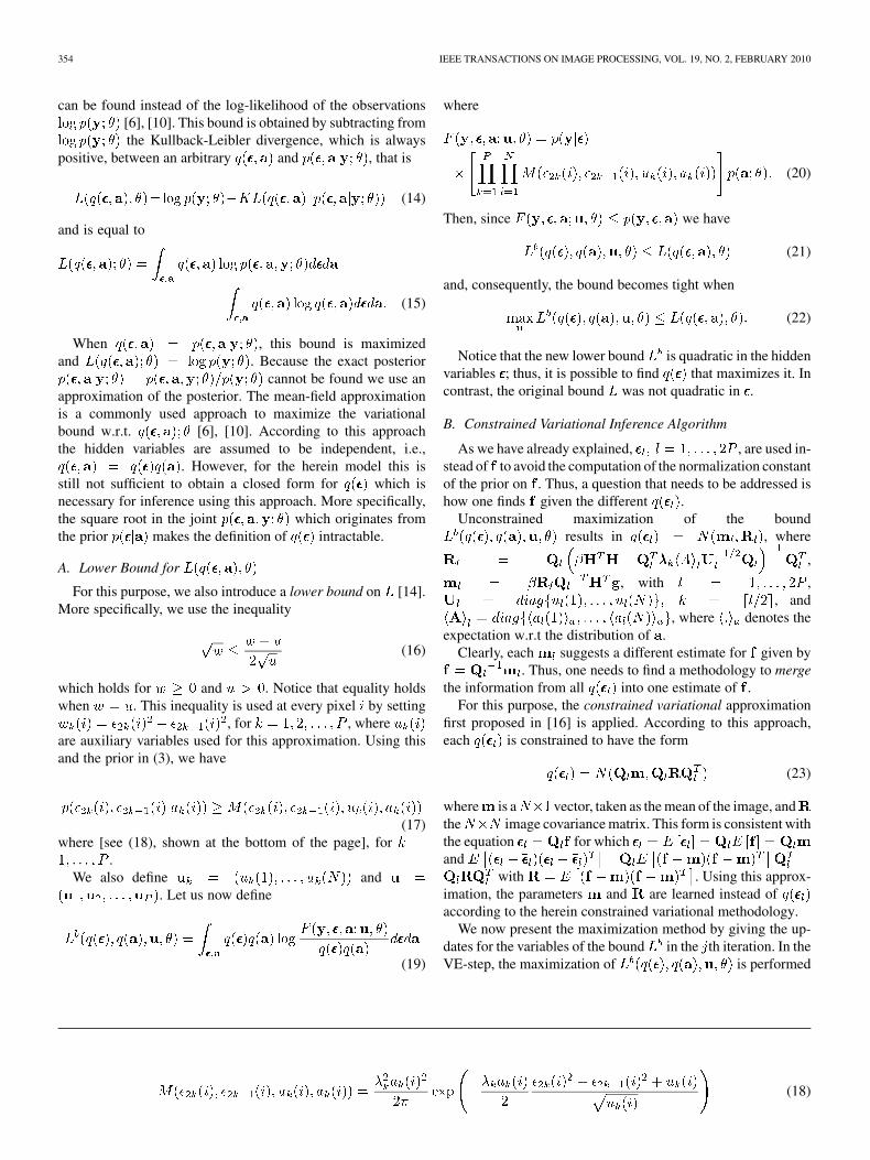
Fig. 1. Magnitude of frequency responses of the filters used in the prior:(a) and (b) the horizontal and vertical differences� �� , (c)� , and (d)� .

the second one is provided by the TV model. In other words,the spatial adaptivity matrix presented in this paper contains,as expected, both regularization mechanisms explained above.Furthermore, due to their TV origin the weights contain the

term in (29) which unlike the “regular” (linear)Student’s-t case contains a square root.

V. COMPUTATIONAL IMPLEMENTATION

Before analyzing the performance of the proposed imagerestoration algorithm, let us discuss important implementationissues. One iteration of the proposed algorithm consists of(27)–(36). The image estimate is taken to be equal to whichis obtained by solving the linear system in (27). The dimensionsof the matrices involved in (27) are , with the numberof pixels in the image. We solve this system iteratively usingthe conjugate-gradient algorithm [22]. We also utilized thismethod to evaluate the diagonal elements of matrix in(29). More specifically, we utilized the -conjugate vectors

for which .Then according to the conjugate-gradient algorithm the imageestimate is updated at every iteration as

where is a scalar [22]. If the method is allowed to iteratetimes we have , where

with all the -conjugate vectors. Thenand the diagonal elements of can

be computed by the formula

(37)

where . In practice the number of iterationsrequired for convergence of the conjugate-gradient methodis much smaller than . We found out that for256 256 images , the conjugate-gradient algo-rithm gives satisfactory results in terms of image restorationwith . An increase of didnot provide much benefit. At this point it is worth also notingthat the Lanczos-based approach which was proposed in [16]required for similar size images to providesimilar restoration results. Thus, the herein proposed algorithmis faster than the algorithm in [16].

In [14], where the diagonal elements of matrices of similarstructure appear in the computation of the restored image, a cir-culant approximation was used. This approximation implies thatall diagonal elements have the same value. In [14], this value


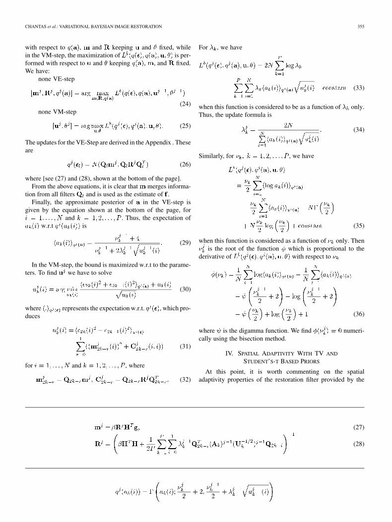
Fig. 2. Experiment on Lena image with Gaussian blur (variance 9) and �� dB; ISNR comparison: (a) Degraded image, (b) restored with spatiallyinvariant prior, [19], �� dB, (c) restored image with method in [16], �� dB, (d) restored image with the proposed algorithm, ��

�� dB.

was set in a trial and error manner. We found out that the ob-tained restoration results using the values of as com-puted by the herein proposed conjugate-gradient approach arenoticeable better than using a circulant approximation for oromitting the elements from (31).

The termination criterion we chose is given by

(38)

where is the image estimate at the th iteration and it is thesolution of the linear system that the con-jugate-gradients algorithm solves. This termination criterion isheuristic. We observed that as the residual of the conjugate gra-dient algorithm increased the restoration quality decreased.

The algorithm is initialized by the resulting image estimateof a Bayesian algorithm that uses a spatially invariant simulta-neously autoregressive image prior [19]. In other words, we setthe initial image estimate equal to the restored image by thisalgorithm. The noise precision is also estimated by the algo-rithm in [19] and we fix it to this value for the remaining of ouralgorithm. Thus, the overall algorithm can be summarized in thefollowing steps.

• Initialize and with the algorithm using a stationaryprior.

• Until convergence do1. Update the parameters , and from (31), (34) and

(36), respectively.2. Update the image estimate from (27) along with

the diagonal elements of in (37).3. Check for convergence using (38).

VI. NUMERICAL EXPERIMENTS

We demonstrate the value of the proposed restoration ap-proach by testing it in experiments with three well known256 256 input images: Lena, Cameraman and Barbara andone 512 512 image USC-man. Every image is blurred withtwo types of blur; the first blur has the shape of a Gaussianfunction with shape parameter 9, and the second is uniformwith support a rectangular region of dimensions 9 9. Theblurred signal to noise ratio was used to quantify thenoise level


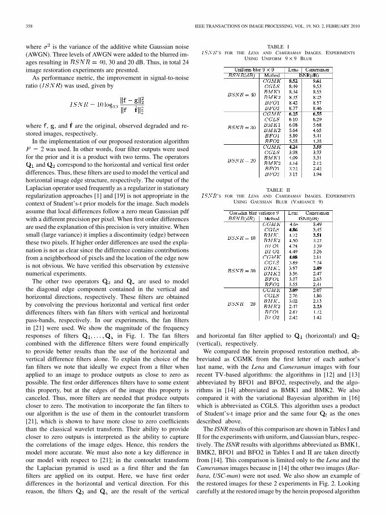
where is the variance of the additive white Gaussian noise(AWGN). Three levels of AWGN were added to the blurred im-ages resulting in , 30 and 20 dB. Thus, in total 24image restoration experiments are presnted.

As performance metric, the improvement in signal-to-noiseratio ( ) was used, given by

where , , and are the original, observed degraded and re-stored images, respectively.

In the implementation of our proposed restoration algorithmwas used. In other words, four filter outputs were used

for the prior and it is a product with two terms. The operatorsand correspond to the horizontal and vertical first order

differences. Thus, these filters are used to model the vertical andhorizontal image edge structure, respectively. The output of theLaplacian operator used frequently as a regularizer in stationaryregularization approaches [1] and [19] is not appropriate in thecontext of Student’s-t prior models for the image. Such modelsassume that local differences follow a zero mean Gaussian pdfwith a different precision per pixel. When first order differencesare used the explanation of this precision is very intuitive. Whensmall (large variance) it implies a discontinuity (edge) betweenthese two pixels. If higher order differences are used the expla-nation is not as clear since the difference contains contributionsfrom a neighborhood of pixels and the location of the edge nowis not obvious. We have verified this observation by extensivenumerical experiments.

The other two operators and are used to modelthe diagonal edge component contained in the vertical andhorizontal directions, respectively. These filters are obtainedby convolving the previous horizontal and vertical first orderdifferences filters with fan filters with vertical and horizontalpass-bands, respectively. In our experiments, the fan filtersin [21] were used. We show the magnitude of the frequencyresponses of filters in Fig. 1. The fan filterscombined with the difference filters were found empiricallyto provide better results than the use of the horizontal andvertical difference filters alone. To explain the choice of thefan filters we note that ideally we expect from a filter whenapplied to an image to produce outputs as close to zero aspossible. The first order differences filters have to some extentthis property, but at the edges of the image this property iscanceled. Thus, more filters are needed that produce outputscloser to zero. The motivation to incorporate the fan filters toour algorithm is the use of them in the contourlet transform[21], which is shown to have more close to zero coefficientsthan the classical wavelet transform. Their ability to providecloser to zero outputs is interpreted as the ability to capturethe correlations of the image edges. Hence, this renders themodel more accurate. We must also note a key difference inour model with respect to [21]; in the contourlet transformthe Laplacian pyramid is used as a first filter and the fanfilters are applied on its output. Here, we have first orderdifferences in the horizontal and vertical direction. For thisreason, the filters and are the result of the vertical

TABLE I��’S FOR THE LENA AND CAMERAMAN IMAGES. EXPERIMENTS

USING UNIFORM 9� 9 BLUR

TABLE II��’S FOR THE LENA AND CAMERAMAN IMAGES. EXPERIMENTS

USING GAUSSIAN BLUR (VARIANCE 9)

and horizontal fan filter applied to (horizontal) and(vertical), respectively.

We compared the herein proposed restoration method, ab-breviated as CGMK from the first letter of each author’slast name, with the Lena and Cameraman images with fourrecent TV-based algorithms: the algorithms in [12] and [13]abbreviated by BFO1 and BFO2, respectively, and the algo-rithms in [14] abbreviated as BMK1 and BMK2. We alsocompared it with the variational Bayesian algorithm in [16]which is abbreviated as CGLS. This algorithm uses a productof Student’s-t image prior and the same four as the onesdescribed above.

The ISNR results of this comparison are shown in Tables I andII for the experiments with uniform, and Gaussian blurs, respec-tively. The ISNR results with algorithms abbreviated as BMK1,BMK2, BFO1 and BFO2 in Tables I and II are taken directlyfrom [14]. This comparison is limited only to the Lena and theCameraman images because in [14] the other two images (Bar-bara, USC-man) were not used. We also show an example ofthe restored images for these 2 experiments in Fig. 2. Lookingcarefully at the restored image by the herein proposed algorithm


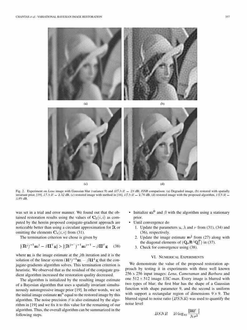
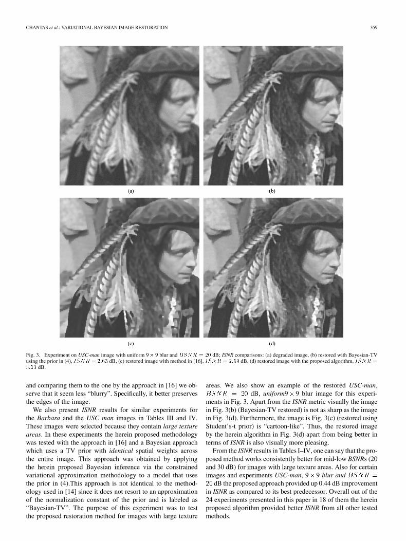
Fig. 3. Experiment on USC-man image with uniform 9� 9 blur and �� dB; ISNR comparisons: (a) degraded image, (b) restored with Bayesian-TVusing the prior in (4), �� dB, (c) restored image with method in [16], �� dB, (d) restored image with the proposed algorithm, ��

�� dB.

and comparing them to the one by the approach in [16] we ob-serve that it seem less “blurry”. Specifically, it better preservesthe edges of the image.

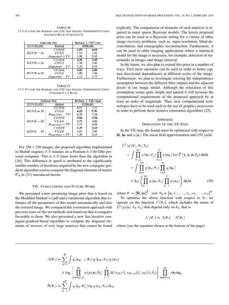
We also present ISNR results for similar experiments forthe Barbara and the USC man images in Tables III and IV.These images were selected because they contain large textureareas. In these experiments the herein proposed methodologywas tested with the approach in [16] and a Bayesian approachwhich uses a TV prior with identical spatial weights acrossthe entire image. This approach was obtained by applyingthe herein proposed Bayesian inference via the constrainedvariational approximation methodology to a model that usesthe prior in (4).This approach is not identical to the method-ology used in [14] since it does not resort to an approximationof the normalization constant of the prior and is labeled as“Bayesian-TV”. The purpose of this experiment was to testthe proposed restoration method for images with large texture

areas. We also show an example of the restored USC-man,dB, uniform9 9 blur image for this experi-

ments in Fig. 3. Apart from the ISNR metric visually the imagein Fig. 3(b) (Bayesian-TV restored) is not as sharp as the imagein Fig. 3(d). Furthermore, the image is Fig. 3(c) (restored usingStudent’s-t prior) is “cartoon-like”. Thus, the restored imageby the herein algorithm in Fig. 3(d) apart from being better interms of ISNR is also visually more pleasing.

From the ISNR results in Tables I–IV, one can say that the pro-posed method works consistently better for mid-low BSNRs (20and 30 dB) for images with large texture areas. Also for certainimages and experiments USC-man, 9 9 blur and

dB the proposed approach provided up 0.44 dB improvementin ISNR as compared to its best predecessor. Overall out of the24 experiments presented in this paper in 18 of them the hereinproposed algorithm provided better ISNR from all other testedmethods.


TABLE III��’S FOR THE BARBARA AND USC-MAN IMAGES. EXPERIMENTS USING

GAUSSIAN BLUR (VARIANCE 9)

TABLE IV��’S FOR THE BARBARA AND USC-MAN IMAGES. EXPERIMENTS USING

UNIFORM 9� 9 BLUR.

For 256 256 images, the proposed algorithm implementedin Matlab requires 3–5 minutes on a Pentium 4 3.40 GHz per-sonal computer. This is 2–5 times faster than the algorithm in[16]. This difference in speed is attributed to the significantlysmaller number of iterations required by the new conjugate-gra-dient algorithm used to compute the diagonal elements of matrix

in (31) introduced herein.

VII. CONCLUSIONS AND FUTURE WORK

We presented a new promising image prior that is based onthe Modified Student’s-t pdf and a variational algorithm that es-timates all the parameters of this model automatically and alsothe restored image. We compared this restoration approach withprevious state-of-the-art methods and found out that it comparesfavorably to them. We also presented a new fast iterative con-jugate-gradient-based algorithm to compute the diagonal ele-ments of inverses of very large matrices that cannot be found

explicitly. The computation of elements of such matrices is re-quired in many sparse Bayesian models. The herein proposedprior can be used in a Bayesian setting for a variety of otherimage recovery problems, such as, super-resolution, blind-de-convolution, and tomographic reconstruction. Furthermore, itcan be used in other imaging applications where a statisticalmodel for the image is necessary, for example, detection of wa-termarks in images and image retrieval.

In the future, we also plan to extend this prior in a number ofways. First more operators can be used in order to better cap-ture directional dependencies at different scales of the image.Furthermore, we plan to investigate relaxing the independenceassumption between the different filter outputs and the adjacentpixels in our image model. Although the relaxation of thisassumption seems quite simple and natural it will increase thecomputational requirements of the proposed approach by atleast an order of magnitude. Thus, new computational tech-nologies have to be used such as the use of graphics processorsin order to perform these iterative restoration algorithms [25].

APPENDIX

DERIVATION OF THE VE-STEP

In the VE-step, the bound must be optimized with respect to, and . The mean field approximation and (19) yield

(39)

whereTo optimize the above function with respect to , we

operate on the function , which includes the terms ofthat depend only on , that is

where (see the equation shown at the bottom of the page).


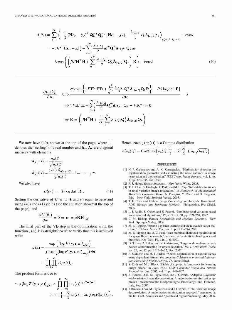
(40)

We now have (40), shown at the top of the page, wheredenotes the “ceiling” of a real number and , are diagonalmatrices with elements

We also have

(41)

Setting the derivative of w.r.t and equal to zero andusing (40) and (41) yields (see the equation shown at the top ofthe page), and

The final part of the VE-step is the optimization w.r.t. thefunction . It is straightforward to verify that this is achievedwhen

The product form is due to

Hence, each is a Gamma distribution

REFERENCES

[1] N. P. Galatsanos and A. K. Katsaggelos, “Methods for choosing theregularization parameter and estimating the noise variance in imagerestoration and their relation,” IEEE Trans. Image Process., vol. 1, no.3, pp. 322–336, Jul. 1992.

[2] P. J. Huber, Robust Statistics. New York: Wiley, 2003.[3] T. F. Chan, S. Esedoglu, F. Park, and M. H. Yip, “Recent developments

in total variation image restoration,” in Handbook of MathematicalModels in Computer Vision, N. Paragios, Y. Chen, and O. Faugeras,Eds. New York: Springer Verlag, 2005.

[4] T. F. Chan and J. Shen, Image Processing and Analysis: Variational,PDE, Wavelet, and Stochastic Methods. Philadelphia, PA: SIAM,2005.

[5] L. I. Rudin, S. Osher, and E. Fatemi, “Nonlinear total variation basednoise removal algorithms,” Phys. D, vol. 60, pp. 259–268, 1992.

[6] C. M. Bishop, Pattern Recognition and Machine Learning. NewYork: Springer Verlag, 2006.

[7] M. E. Tipping, “Sparse Bayesian learning and the relevance vector ma-chine,” J. Mach. Learn. Res., vol. 1, pp. 211–244, 2001.

[8] M. E. Tipping and A. C. Faul, “Fast marginal likelihood maximisationfor sparse Bayesian models,” presented at the Artificial Intelligence andStatistics, Key West, FL, Jan. 3–6, 2003.

[9] D. Tzikas, A. Likas, and N. Galatsanos, “Large scale multikernel rel-evance vector machine for object detection,” Int. J. Artif. Intell. Tools,vol. 26, no. 12, pp. 1613–1622, Dec. 2007.

[10] E. Sudderth and M. I. Jordan, “Shared segmentation of natural scenesusing dependent Pitman-Yor processes,” Advances in Neural Informa-tion Processing Systems (NIPS) 21, unpublished.

[11] S. Roth and M. J. Black, “Fields of experts: A framework for learningimage priors,” in Proc. IEEE Conf. Computer Vision and PatternRecognition, Jun. 2005, vol. II, pp. 860–867.

[12] J. Bioucas-Dias, M. Figueiredo, and J. Oliveira, “Adaptive Bayesian/total-variation image deconvolution: A majorization-minimization ap-proach,” presented at the European Signal Processing Conf., Florence,Italy, Sep. 2006.

[13] J. Bioucas-Dias, M. Figueiredo, and J. Oliveira, “Total-variation imagedeconvolution: A majorization-minimization approach,” presented atthe Int. Conf. Acoustics and Speech and Signal Processing, May 2006.


[14] S. D. Babacan, R. Molina, and A. K. Katsaggelos, “Parameter estima-tion in TV image restoration using variational distribution approxima-tion,” IEEE Trans. Image Process., vol. 17, no. 3, pp. 326–339, Mar.2008.

[15] G. Chantas, N. P. Galatsanos, and A. Likas, “Bayesian restoration usinga new non-stationary edge-preserving image prior,” IEEE Trans. ImageProcess., vol. 15, no. 10, pp. 2987–2997, Oct. 2006.

[16] G. Chantas, N. P. Galatsanos, A. Likas, and M. Saunders, “VariationalBayesian image restoration based on a product of t-distributions imageprior,” IEEE Trans. Image Process., vol. 17, no. 10, pp. 1795–1805,Oct. 2008.

[17] S. D. Babacan, R. Molina, and A. K. Katsaggelos, “VariationalBayesian blind deconvolution using a total variation prior,” IEEETrans. Image Process., vol. 18, no. 1, pp. 12–26, Jan. 2009.

[18] D. G. Tzikas, A. C. Likas, and N. P. Galatsanos, “Variational Bayesiansparse kernel-based blind image deconvolution with student’s-t priors,”IEEE Trans. Image Process., vol. 18, no. 4, pp. 753–764, Apr. 2009.

[19] R. Molina, A. K. Katsaggelos, and J. Mateos, “Bayesian and regular-ization methods for hyper-parameter estimation in image restoration,”IEEE Trans. Image Process., vol. 8, no. 2, pp. 231–246, Feb. 1999.

[20] K. Lang, Lange, Optimization, Spinger Texts in Statistics. New York:Springer-Verlag, 2004.

[21] A. L. Cunha, J. Zhou, and M. N. Do, “The nonsubsampled contourlettransform: Theory, design, and applications,” IEEE Trans. ImageProcess., vol. 15, no. 10, pp. 3089–3101, Oct. 2006.

[22] Y. Saad, Iterative Methods for Sparse Linear Systems, 2nded. Philadelphia, PA: SIAM, 2000.

[23] D. Sun and W.-K. Cham, “Postprocessing of low bit-rate block dctcoded images based on a fields of experts prior,” IEEE Trans. ImageProcess., vol. 16, no. 11, pp. 2743–2751, Nov. 2007.

[24] M. Bertalmio, V. Caselles, B. Rougé, and A. Solé, “TV based imagerestoration with local constraints,” J. Sci. Comput., vol. 19, no. 1, pp.95–122, Dec. 2003.

[25] J. Fung and S. Mann, “Using graphics devices in reverse: GPU-basedimage processing and computer vision,” in Proc. IEEE Int. Conf. Mul-timedia and Expo, Jun. 26, 2008, pp. 9–12.

Giannis Chantas received the Diploma degree incomputer science in 2002, the M.S. degree in 2004,and the Ph.D degree from the University of Ioannina,Ioannina, Greece.

He is currently with the Technological EducationalInstitute of Informatics and Telecommunications,Larissa, Greece. His research interests are in thearea of statistical image processing and includeBayesian image restoration, blind deconvolution,and super-resolution.

Nikolas P. Galatsanos (SM’95) received theDiploma of Electrical Engineering from the NationalTechnical University of Athens, Greece, in 1982, andthe M.S.E.E. and Ph.D. degrees from the Electricaland Computer Engineering Department, Universityof Wisconsin, Madison, in 1984 and 1989, respec-tively.

He was on the faculty of the Electrical andComputer Engineering Department, Illinois Instituteof Technology, Chicago, from 1989 to 2002. Hewas with the Department of Computer Science,

University of Ioannina, Ioannina, Greece, from 2002–2008. Presently, he iswith the Department of Electrical and Computer Engineering, University ofPatras, Patras, Greece. He coedited a book titled Image Recovery Techniques forImage and Video Compression and Transmission (Kluwer, 1998). His researchinterests center around image processing and statistical learning problems formedical imaging and visual communications applications.

Dr. Galatsanos has served as an Associate Editor for the IEEE TRANSACTIONS

ON IMAGE PROCESSING and the IEEE Signal Processing Magazine, and heserved as an Associate Editor for the Journal of Electronic Imaging.

Rafael Molina was born in 1957. He received the de-gree in mathematics (statistics) in 1979 and the Ph.D.degree in optimal design in linear models in 1983.

He became Professor of computer science andartificial intelligence at the University of Granada,Granada, Spain, in 2000. His areas of researchinterest are image restoration (applications to as-tronomy and medicine), parameter estimation inimage restoration, super resolution of images andvideo, computational photography, compressivesensing, and blind deconvolution.

Aggelos K. Katsaggelos (S’80–M’85–SM’92–F’98)received the Diploma degree in electrical and me-chanical engineering from the Aristotelian Universityof Thessaloniki, Thessaloniki, Greece, in 1979, andthe M.S. and Ph.D. degrees in electrical engineeringfrom the Georgia Institute of Technology, Atlanta, in1981 and 1985, respectively.

In 1985, he joined the Department of Electricaland Computer Engineering, Northwestern Univer-sity, Evanston, IL, where he is currently a Professor.He held the Ameritech Chair of Information Tech-

nology from 1997 to 2003. He is also the Director of the Motorola Center forCommunications and a member of the Academic Affiliate Staff, Departmentof Medicine, Evanston Hospital. He is the editor of Digital Image Restoration(Springer-Verlag, 1991), coauthor of Rate-Distortion Based Video Compres-sion (Kluwer, 1997), coeditor of Recovery Techniques for Image and VideoCompression and Transmission (Kluwer, 1998), and co author of Super-Reso-lution for Images and Video (Claypool, 2007) and Joint Source-Channel VideoTransmission (Claypool, 2007), as well as the coinventor of 12 patents.

Dr. Katsaggelos has served the IEEE and other professional societies inmany capacities. For example, he was Editor-in-Chief of the IEEE SignalProcessing Magazine (1997–2002), a member of the Board of Governors of theIEEE Signal Processing Society (1999–2001), and a member of the PublicationBoard of the IEEE PROCEEDINGS (2003–2007). He is the recipient of theIEEE Third Millennium Medal (2000), the IEEE Signal Processing SocietyMeritorious Service Award (2001), an IEEE Signal Processing Society BestPaper Award (2001), an IEEE International Conference on Multimedia andExpo Paper Award (2006), and an IEEE International Conference on ImageProcessing Paper Award (2007). He is a Distinguished Lecturer of the IEEESignal Processing Society (2007–2008).

Variational Bayesian Image Restoration With a Product of Spatially Weighted Total Variation Image...

Documents

Transcript of Variational Bayesian Image Restoration With a Product of Spatially Weighted Total Variation Image...