Scene Shape Priors for Superpixel Segmentation

Alastair P. Moore Simon J. D. Prince∗ Jonathan Warrell∗ Umar Mohammed Graham Jones†

University College LondonGower Street, WC1E 6BT, UK

{a.moore,s.prince}@cs.ucl.ac.uk

† Sharp Laboratories EuropeOxford, OX4 4GB, UK

graham.jones@sharp.co.uk

Abstract

Unsupervised over-segmentation of an image into super-pixels is a common preprocessing step for image parsingalgorithms. Superpixels are used as both regions of sup-port for feature vectors and as a starting point for the fi-nal segmentation. In this paper we investigate incorporat-ing a priori information into superpixel segmentations. Welearn a probabilistic model that describes the spatial den-sity of the object boundaries in the image. We then describean over-segmentation algorithm that partitions this densityroughly equally between superpixels whilst still attemptingto capture local object boundaries. We demonstrate this ap-proach using road scenes where objects in the center of theimage tend to be more distant and smaller than those at theedge. We show that our algorithm successfully learns thisfoveated spatial distribution and can exploit this knowledgeto improve the segmentation. Lastly, we introduce a newmetric for evaluating vision labeling problems. We measureperformance on a challenging real-world dataset and illus-trate the limitations of conventional evaluation metrics.

1. IntroductionSegmentation is a well studied problem and there has

been much recent progress in supervised/user guided al-gorithms. However a solution to achieving good unsuper-vised segmentation remains elusive and performance onreal-world datasets is low [5]. This is in part due to thefact that it is difficult to separate the processes of segmen-tation, detection and recognition: In the absence of sim-ple metrics of homogeneity it is impossible to segment anobject in a scene without having first located it (detection)and estimated some of its properties (recognition). Whilesome effort has been made on combining these separate pro-cesses [11, 21] the variations that result from occlusion andchanges of pose and lighting make this a challenging task.

Despite this difficulty recent progress has been madeby oversegmenting the image. Small regions of the im-

∗We acknowledge the support of the EPSRC Grant No. EP/E013309/1.

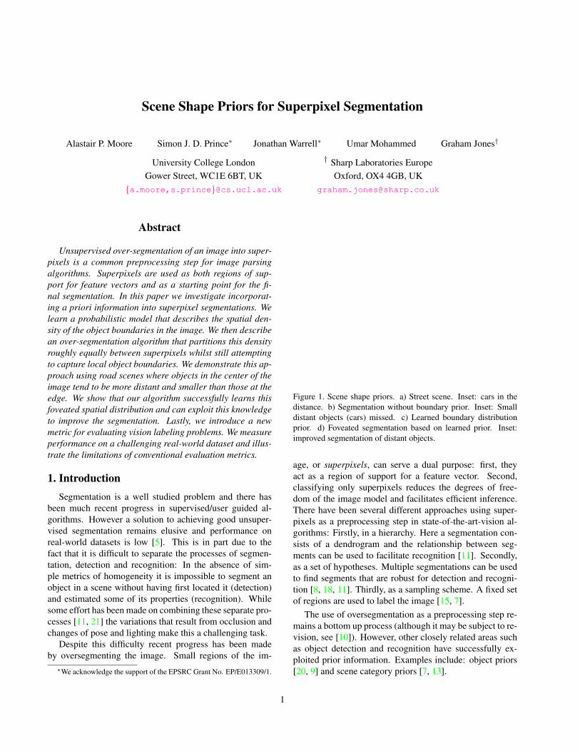
Figure 1. Scene shape priors. a) Street scene. Inset: cars in thedistance. b) Segmentation without boundary prior. Inset: Smalldistant objects (cars) missed. c) Learned boundary distributionprior. d) Foveated segmentation based on learned prior. Inset:improved segmentation of distant objects.

age, or superpixels, can serve a dual purpose: first, theyact as a region of support for a feature vector. Second,classifying only superpixels reduces the degrees of free-dom of the image model and facilitates efficient inference.There have been several different approaches using super-pixels as a preprocessing step in state-of-the-art-vision al-gorithms: Firstly, in a hierarchy. Here a segmentation con-sists of a dendrogram and the relationship between seg-ments can be used to facilitate recognition [11]. Secondly,as a set of hypotheses. Multiple segmentations can be usedto find segments that are robust for detection and recogni-tion [8, 18, 11]. Thirdly, as a sampling scheme. A fixed setof regions are used to label the image [15, 7].

The use of oversegmentation as a preprocessing step re-mains a bottom up process (although it may be subject to re-vision, see [10]). However, other closely related areas suchas object detection and recognition have successfully ex-ploited prior information. Examples include: object priors[20, 9] and scene category priors [7, 13].

1

In contrast there has been very little work on incorporat-ing priors in the process of oversegmentation. For instancewhile it is noted in [6] that it is possible to have the segmen-tation method prefer components of certain size or shapethis is not exploited. In [15] uniform size superpixels areencouraged using postprocessing regardless of where theyappear in the image. Similarly, the algorithm presented in[14] implicitly assumes scenes that are largely frontoplanaror that objects of interest are reasonably large in the im-age. Alternatively there has been work placing priors onsuperpixels [8, 12] without it guiding the segmentation pro-cess itself. It remains to be seen whether it is possible toachieve good recognition rates without performing segmen-tation but in this paper we advocate an approach that usespriors in the process of oversegmentation. An example ofone such spatial prior is shown in Figure 1.

The contributions of the paper are as follows: In Sec-tion 3 we describe an algorithm that uses an estimate of thedistribution of boundaries in an image for foveation of thesegmentation. In Section 4 we learn a model for the dis-tribution of boundaries in an image from training data. InSection 5 we introduce a new metric for evaluating segmen-tation algorithms.

2. Superpixel LatticesWe begin by describing an existing superpixel lattice al-

gorithm [14] and highlight its limitations. This motivatesthe use of priors in over-segmentation. In Section 3 weadapt this method to incorporate such prior information.

The superpixel lattice algorithm [14] divides the imageinto a regular grid of superpixels. The input to the algo-rithm is a boundary map. This is a 2D array containing ameasure of the probability that a semantically meaningfulboundary is present between two pixels. The boundary mapis then inverted to take a value of 0 where there is the mostevidence for a boundary and 1 where there is no evidence.This inverted map is called the boundary cost map.

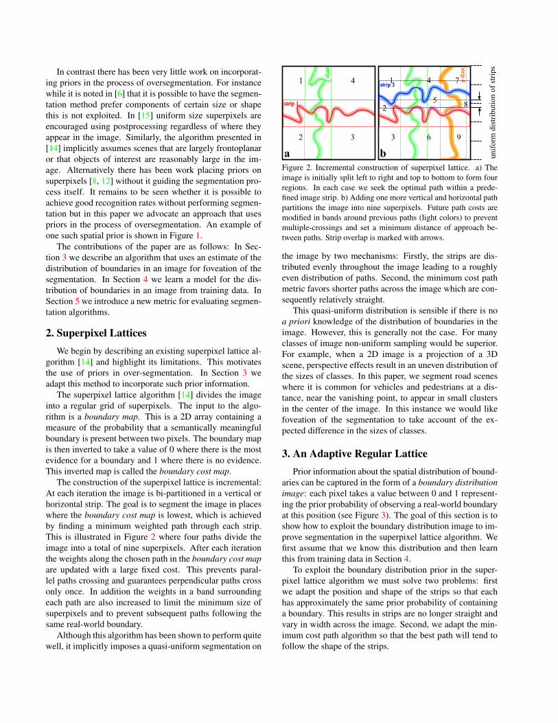
The construction of the superpixel lattice is incremental:At each iteration the image is bi-partitioned in a vertical orhorizontal strip. The goal is to segment the image in placeswhere the boundary cost map is lowest, which is achievedby finding a minimum weighted path through each strip.This is illustrated in Figure 2 where four paths divide theimage into a total of nine superpixels. After each iterationthe weights along the chosen path in the boundary cost mapare updated with a large fixed cost. This prevents paral-lel paths crossing and guarantees perpendicular paths crossonly once. In addition the weights in a band surroundingeach path are also increased to limit the minimum size ofsuperpixels and to prevent subsequent paths following thesame real-world boundary.

Although this algorithm has been shown to perform quitewell, it implicitly imposes a quasi-uniform segmentation on

Figure 2. Incremental construction of superpixel lattice. a) Theimage is initially split left to right and top to bottom to form fourregions. In each case we seek the optimal path within a prede-fined image strip. b) Adding one more vertical and horizontal pathpartitions the image into nine superpixels. Future path costs aremodified in bands around previous paths (light colors) to preventmultiple-crossings and set a minimum distance of approach be-tween paths. Strip overlap is marked with arrows.

the image by two mechanisms: Firstly, the strips are dis-tributed evenly throughout the image leading to a roughlyeven distribution of paths. Second, the minimum cost pathmetric favors shorter paths across the image which are con-sequently relatively straight.

This quasi-uniform distribution is sensible if there is noa priori knowledge of the distribution of boundaries in theimage. However, this is generally not the case. For manyclasses of image non-uniform sampling would be superior.For example, when a 2D image is a projection of a 3Dscene, perspective effects result in an uneven distribution ofthe sizes of classes. In this paper, we segment road sceneswhere it is common for vehicles and pedestrians at a dis-tance, near the vanishing point, to appear in small clustersin the center of the image. In this instance we would likefoveation of the segmentation to take account of the ex-pected difference in the sizes of classes.

3. An Adaptive Regular LatticePrior information about the spatial distribution of bound-

aries can be captured in the form of a boundary distributionimage: each pixel takes a value between 0 and 1 represent-ing the prior probability of observing a real-world boundaryat this position (see Figure 3). The goal of this section is toshow how to exploit the boundary distribution image to im-prove segmentation in the superpixel lattice algorithm. Wefirst assume that we know this distribution and then learnthis from training data in Section 4.

To exploit the boundary distribution prior in the super-pixel lattice algorithm we must solve two problems: firstwe adapt the position and shape of the strips so that eachhas approximately the same prior probability of containinga boundary. This results in strips are no longer straight andvary in width across the image. Second, we adapt the min-imum cost path algorithm so that the best path will tend tofollow the shape of the strips.

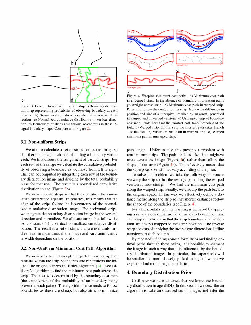
Figure 3. Construction of non-uniform strip a) Boundary distribu-tion map representing probability of observing boundary at eachposition. b) Normalized cumulative distribution in horizontal di-rection. c) Normalized cumulative distribution in vertical direc-tion. d) Boundaries of strips now follow iso-contours in these in-tegral boundary maps. Compare with Figure 2a.

3.1. Non-uniform Strips

We aim to calculate a set of strips across the image sothat there is an equal chance of finding a boundary withineach. We first discuss the assignment of vertical strips. Foreach row of the image we calculate the cumulative probabil-ity of observing a boundary as we move from left to right.This can be computed by integrating each row of the bound-ary distribution image and dividing by the total probabilitymass for that row. The result is a normalized cumulativedistribution image (Figure 3b).

We now allocate strips so that they partition the cumu-lative distribution equally. In practice, this means that theedge of the strips follow the iso-contours of the normal-ized cumulative distribution image. For horizontal strips,we integrate the boundary distribution image in the verticaldirection and normalize. We allocate strips that follow theiso-contours of this vertical normalized cumulative distri-bution. The result is a set of strips that are non-uniform -they may meander through the image and vary significantlyin width depending on the position.

3.2. Non-Uniform Minimum Cost Path Algorithm

We now seek to find an optimal path for each strip thatremains within the strip boundaries and bipartitions the im-age. The original superpixel lattice algorithm [14] used Di-jkstra’s algorithm to find the minimum cost path across thestrip. The cost was determined by the boundary cost map(the complement of the probability of an boundary beingpresent at each point). The algorithm hence tends to followboundaries as these are cheap, but also aims to minimize

Figure 4. Warping minimum cost paths. a) Minimum cost pathin unwarped strip. In the absence of boundary information pathsgo straight across strip. b) Minimum cost path in warped strip.Paths will follow the contour of the strip. Notice the difference inposition and size of a superpixel, marked by an arrow, generatedin warped and unwarped versions. c) Unwarped strip of boundarycost map. Note here that the shortest path takes branch 2 of thefork. d) Warped strip. In this strip the shortest path takes branch1 of the fork. e) Minimum cost path in warped strip. d) Warpedminimum path in unwarped strip.

path length. Unfortunately, this presents a problem withnon-uniform strips. The path tends to take the straightestroute across the image (Figure 4a) rather than follow theshape of the strip (Figure 4b). This effectively means thatthe superpixel size will not vary according to the prior.

To solve this problem we take the following approach:we warp the strip so that the average path along the warpedversion is now straight. We find the minimum cost pathalong the warped strip. Finally, we unwarp the path back tothe original space. In this way we effectively define a dis-tance metric along the strip so that shorter distances followthe shape of the boundaries (see Figure 4).

For a horizontal strip, the warping is achieved by apply-ing a separate one dimensional affine warp to each column.The warps are chosen so that the strip boundaries in that col-umn are always mapped to the same position. The inversewarp consists of applying the inverse one dimensional affinetransform to each column.

By repeatedly finding non-uniform strips and finding op-timal paths through these strips, it is possible to segmentthe image in such a way that it is influenced by the bound-ary distribution image. In particular, the superpixels willbe smaller and more densely packed in regions where weexpect to find more image boundaries.

4. Boundary Distribution Prior

Until now we have assumed that we know the bound-ary distribution image (BDI). In this section we describe analgorithm to take an observed set of images and infer the

most likely boundary distribution image. The image willdepend on both prior information about the spatial statisticsof boundaries (learnt from training data) and the observededge data from a particular image. In this section we de-scribe the model before describing learning (Section 4.1)and inference (Section 4.2) algorithms.

We wish to describe a probability distribution over ob-served boundaries x = [x1 . . . xP ]T at the p pixels of animage. Each element xp is binary and is 1 when a bound-ary is present and 0 when it is absent. We assumes that xpis drawn from a single observation of a binomial distribu-tion with parameter yp. Our goal then is to model the jointprobability distribution of the vector of binomial parametersy = [y1 . . . yP ]T . The vector y represents the boundary dis-tribution image or BDI.

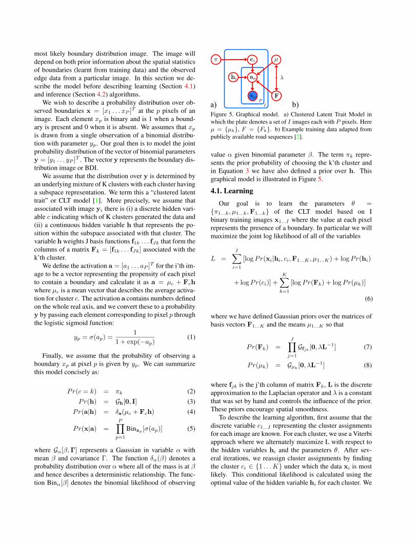
We assume that the distribution over y is determined byan underlying mixture of K clusters with each cluster havinga subspace representation. We term this a “clustered latenttrait” or CLT model [1]. More precisely, we assume thatassociated with image yi there is (i) a discrete hidden vari-able c indicating which of K clusters generated the data and(ii) a continuous hidden variable h that represents the po-sition within the subspace associated with that cluster. Thevariable h weights J basis functions f1k . . . fJk that form thecolumns of a matrix Fk = [f1k . . . fJk] associated with thek’th cluster.

We define the activation a = [a1 . . . aP ]T for the i’th im-age to be a vector representing the propensity of each pixelto contain a boundary and calculate it as a = µc + Fchwhere µc is a mean vector that describes the average activa-tion for cluster c. The activation a contains numbers definedon the whole real axis, and we convert these to a probabilityy by passing each element corresponding to pixel p throughthe logistic sigmoid function:

yp = σ(ap) =1

1 + exp(−ap)(1)

Finally, we assume that the probability of observing aboundary xp at pixel p is given by yp. We can summarizethis model concisely as:

Pr(c = k) = πk (2)Pr(h) = Gh[0, I] (3)

Pr(a|h) = δa(µc + Fch) (4)

Pr(x|a) =P∏p=1

Binxp [σ(ap)] (5)

where Gα[β,Γ] represents a Gaussian in variable α withmean β and covariance Γ. The function δα(β) denotes aprobability distribution over α where all of the mass is at βand hence describes a deterministic relationship. The func-tion Binα[β] denotes the binomial likelihood of observing

Figure 5. Graphical model. a) Clustered Latent Trait Model inwhich the plate denotes a set of I images each with P pixels. Hereµ = {µk}, F = {Fk}. b) Example training data adapted frompublicly available road sequences [2].

value α given binomial parameter β. The term πk repre-sents the prior probability of choosing the k’th cluster andin Equation 3 we have also defined a prior over h. Thisgraphical model is illustrated in Figure 5.

4.1. Learning

Our goal is to learn the parameters θ ={π1...k, µ1...k,F1...k} of the CLT model based on Ibinary training images x1...I where the value at each pixelrepresents the presence of a boundary. In particular we willmaximize the joint log likelihood of all of the variables

L =I∑i=1

[logPr(xi|hi, ci,F1...K , µ1...K) + logPr(hi)

+ logPr(ci)] +K∑k=1

[logPr(Fk) + logPr(µk)]

(6)

where we have defined Gaussian priors over the matrices ofbasis vectors F1...K and the means µ1...K so that

Pr(Fk) =J∏j=1

Gfjk[0, λL−1] (7)

Pr(µk) = Gµk[0, λL−1] (8)

where fjk is the j’th column of matrix Fk, L is the discreteapproximation to the Laplacian operator and λ is a constantthat was set by hand and controls the influence of the prior.These priors encourage spatial smoothness.

To describe the learning algorithm, first assume that thediscrete variable c1...I representing the cluster assignmentsfor each image are known. For each cluster, we use a Viterbiapproach where we alternately maximize L with respect tothe hidden variables hi and the parameters θ. After sev-eral iterations, we reassign cluster assignments by findingthe cluster ci ∈ {1 . . .K} under which the data xi is mostlikely. This conditional likelihood is calculated using theoptimal value of the hidden variable hi for each cluster. We

Algorithm 1 Learn Clustered Latent Trait Model1: for t1 = 1 to T1 do2: \\ Reassign data to clusters3: for all i do4: ci,hi ← arg maxci,hi

logPr(xi,hi, ci, θ)5: end for6: \\Update parameters for each cluster7: for t2 = 1 to T2 do8: for all k do9: θk ← arg maxθk

∑s∈{s:cs=k} logPr(xs, θ, cs,hs)

10: end for11: for all i do12: hi ← arg maxhi logPr(xi,hi, θ, ci, )13: end for14: end for15: end for16: return θ1...K

also re-estimate the prior probability π1...K of each cluster.Having reassigned the points, we then relearn each clusterseparately and so on. Algorithm 1 describes this processmore formally. The maximization over the discrete param-eters ci was done exhaustively. The maximization over thecontinuous parameters θ and h1...I was performed using aquasi-Newton method. The update for π1 . . . πk is calcu-lated in closed form:

πk =1I

I∑i=1

δ(ci = k) (9)

Examples of the boundary distribution image y associatedwith each cluster mean are illustrated in Figure 6.

4.2. Inference

In this section we describe how to predict the boundarydistribution image that was most likely to have been respon-sible for a new observed image. We calculate a binary edgemap for the new image and use this as a proxy for the un-seen boundary map xt. We then find the the cluster ct andhidden variable ht that were most likely to have created it:

ct,ht ← arg maxct,ht

logPr(xt,ht, ct, θ) (10)

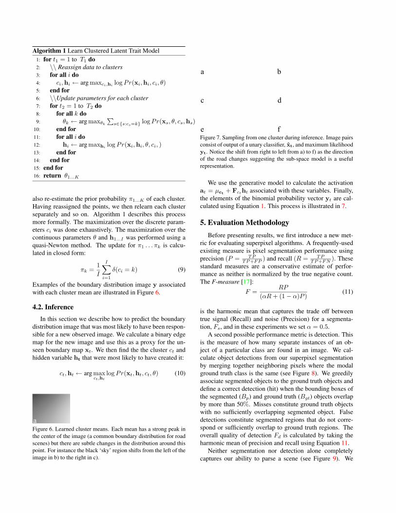
Figure 6. Learned cluster means. Each mean has a strong peak inthe center of the image (a common boundary distribution for roadscenes) but there are subtle changes in the distribution around thispoint. For instance the black ‘sky’ region shifts from the left of theimage in b) to the right in c).

Figure 7. Sampling from one cluster during inference. Image pairsconsist of output of a unary classifier, x̂t, and maximum likelihoodyt. Notice the shift from right to left from a) to f) as the directionof the road changes suggesting the sub-space model is a usefulrepresentation.

We use the generative model to calculate the activationat = µct + Fct

ht associated with these variables. Finally,the elements of the binomial probability vector yt are cal-culated using Equation 1. This process is illustrated in 7.

5. Evaluation MethodologyBefore presenting results, we first introduce a new met-

ric for evaluating superpixel algorithms. A frequently-usedexisting measure is pixel segmentation performance usingprecision (P = TP

TP+FP ) and recall (R = TPTP+FN ). These

standard measures are a conservative estimate of perfor-mance as neither is normalized by the true negative count.The F-measure [17]:

F =RP

(αR+ (1− α)P )(11)

is the harmonic mean that captures the trade off betweentrue signal (Recall) and noise (Precision) for a segmenta-tion, Fs, and in these experiments we set α = 0.5.

A second possible performance metric is detection. Thisis the measure of how many separate instances of an ob-ject of a particular class are found in an image. We cal-culate object detections from our superpixel segmentationby merging together neighboring pixels where the modalground truth class is the same (see Figure 8). We greedilyassociate segmented objects to the ground truth objects anddefine a correct detection (hit) when the bounding boxes ofthe segmented (Bp) and ground truth (Bgt) objects overlapby more than 50%. Misses constitute ground truth objectswith no sufficiently overlapping segmented object. Falsedetections constitute segmented regions that do not corre-spond or sufficiently overlap to ground truth regions. Theoverall quality of detection Fd is calculated by taking theharmonic mean of precision and recall using Equation 11.

Neither segmentation nor detection alone completelycaptures our ability to parse a scene (see Figure 9). We

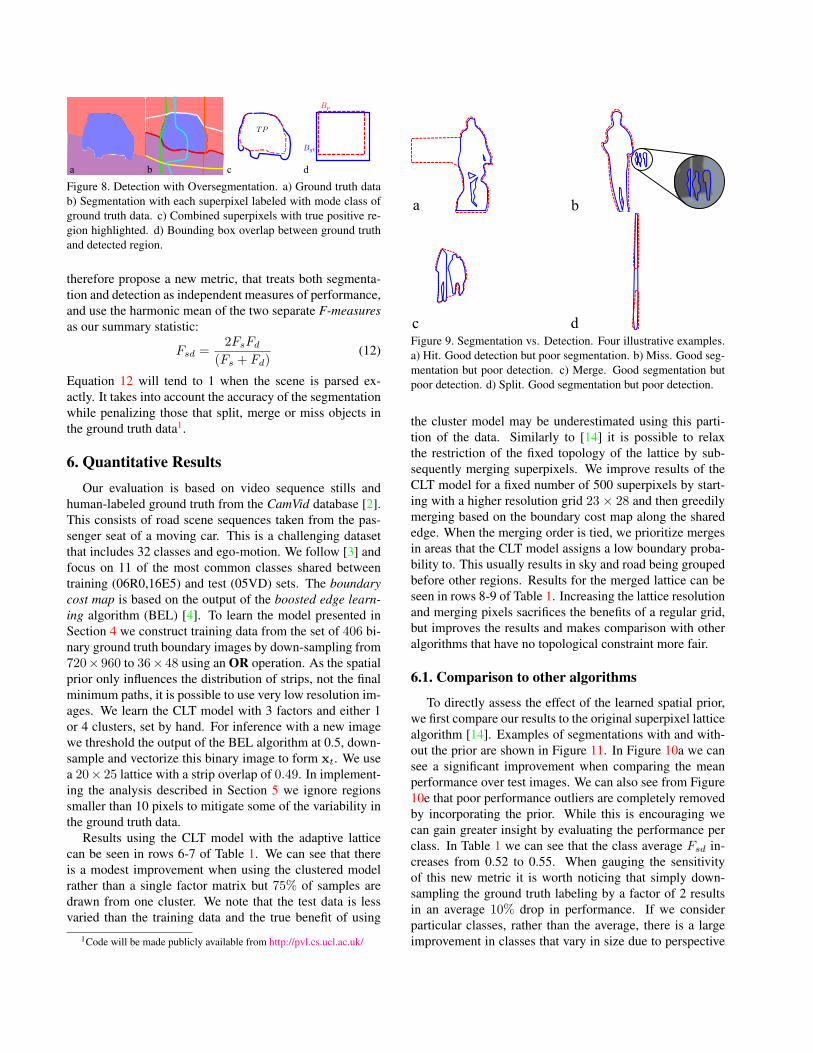
Figure 8. Detection with Oversegmentation. a) Ground truth datab) Segmentation with each superpixel labeled with mode class ofground truth data. c) Combined superpixels with true positive re-gion highlighted. d) Bounding box overlap between ground truthand detected region.

therefore propose a new metric, that treats both segmenta-tion and detection as independent measures of performance,and use the harmonic mean of the two separate F-measuresas our summary statistic:

Fsd =2FsFd

(Fs + Fd)(12)

Equation 12 will tend to 1 when the scene is parsed ex-actly. It takes into account the accuracy of the segmentationwhile penalizing those that split, merge or miss objects inthe ground truth data1.

6. Quantitative ResultsOur evaluation is based on video sequence stills and

human-labeled ground truth from the CamVid database [2].This consists of road scene sequences taken from the pas-senger seat of a moving car. This is a challenging datasetthat includes 32 classes and ego-motion. We follow [3] andfocus on 11 of the most common classes shared betweentraining (06R0,16E5) and test (05VD) sets. The boundarycost map is based on the output of the boosted edge learn-ing algorithm (BEL) [4]. To learn the model presented inSection 4 we construct training data from the set of 406 bi-nary ground truth boundary images by down-sampling from720× 960 to 36× 48 using an OR operation. As the spatialprior only influences the distribution of strips, not the finalminimum paths, it is possible to use very low resolution im-ages. We learn the CLT model with 3 factors and either 1or 4 clusters, set by hand. For inference with a new imagewe threshold the output of the BEL algorithm at 0.5, down-sample and vectorize this binary image to form xt. We usea 20× 25 lattice with a strip overlap of 0.49. In implement-ing the analysis described in Section 5 we ignore regionssmaller than 10 pixels to mitigate some of the variability inthe ground truth data.

Results using the CLT model with the adaptive latticecan be seen in rows 6-7 of Table 1. We can see that thereis a modest improvement when using the clustered modelrather than a single factor matrix but 75% of samples aredrawn from one cluster. We note that the test data is lessvaried than the training data and the true benefit of using

1Code will be made publicly available from http://pvl.cs.ucl.ac.uk/

Figure 9. Segmentation vs. Detection. Four illustrative examples.a) Hit. Good detection but poor segmentation. b) Miss. Good seg-mentation but poor detection. c) Merge. Good segmentation butpoor detection. d) Split. Good segmentation but poor detection.

the cluster model may be underestimated using this parti-tion of the data. Similarly to [14] it is possible to relaxthe restriction of the fixed topology of the lattice by sub-sequently merging superpixels. We improve results of theCLT model for a fixed number of 500 superpixels by start-ing with a higher resolution grid 23× 28 and then greedilymerging based on the boundary cost map along the sharededge. When the merging order is tied, we prioritize mergesin areas that the CLT model assigns a low boundary proba-bility to. This usually results in sky and road being groupedbefore other regions. Results for the merged lattice can beseen in rows 8-9 of Table 1. Increasing the lattice resolutionand merging pixels sacrifices the benefits of a regular grid,but improves the results and makes comparison with otheralgorithms that have no topological constraint more fair.

6.1. Comparison to other algorithms

To directly assess the effect of the learned spatial prior,we first compare our results to the original superpixel latticealgorithm [14]. Examples of segmentations with and with-out the prior are shown in Figure 11. In Figure 10a we cansee a significant improvement when comparing the meanperformance over test images. We can also see from Figure10e that poor performance outliers are completely removedby incorporating the prior. While this is encouraging wecan gain greater insight by evaluating the performance perclass. In Table 1 we can see that the class average Fsd in-creases from 0.52 to 0.55. When gauging the sensitivityof this new metric it is worth noticing that simply down-sampling the ground truth labeling by a factor of 2 resultsin an average 10% drop in performance. If we considerparticular classes, rather than the average, there is a largeimprovement in classes that vary in size due to perspective

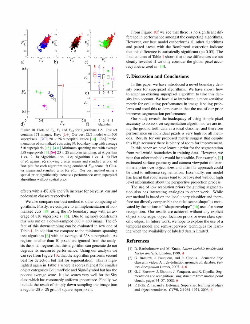
Figure 10. Plots of Fs, Fd and Fsd for algorithms 1-5. Test setcontains 171 images. Key: [1+] Our best CLT model with 500superpixels. [2�] 20 × 25 superpixel lattice [14]. [3�] Imple-mentation of normalized cuts using Pb boundary map with average510 superpixels [15]. [4×] Minimum spanning tree with average558 superpixels [6].[5•] 20× 25 uniform sampling. a) Algorithm1 vs. 2. b) Algorithm 1 vs. 3 c) Algorithm 1 vs. 4. d) Plotof Fs against Fd showing cluster means and standard errors. e)Box plot for each algorithm using combined Fsd score. f) Clus-ter means and standard error for Fsd. Our best method using aspatial prior significantly increases performance over superpixelalgorithms without spatial prior.

effects with a 4%, 8% and 9% increase for bicyclist, car andpedestrian classes respectively.

We also compare our best method to other competing al-gorithms. Firstly, we compare to an implementation of nor-malized cuts [19] using the Pb boundary map with an av-erage of 510 superpixels [15]. Due to memory constraintsthis was run on a down-sampled 360 × 480 image. The ef-fect of this downsampling can be evaluated in row one ofTable 1. In addition we compare to the minimum spanningtree algorithm [6] with an average of 558 superpixels. Asregions smaller than 10 pixels are ignored from the analy-sis the small regions that this algorithm can generate do notdegrade its measured performance. Using our analysis wecan see from Figure 10d that the algorithm performs secondbest for detection but last for segmentation. This is high-lighted again in Table 1 where it scores highest for smallerobject categories Column/Pole and Sign/Symbol but has thepoorest average score. It also scores very well for the Skyclass which has reasonably uniform appearance. Finally, weinclude the result of simply down-sampling the image intoa regular 20× 25 grid of square superpixels.

From Figure 10f we see that there is no significant dif-ference in performance amongst the competing algorithms.However, our best model outperforms all other algorithmsand paired t-tests with the Bonferroni correction indicatethat this difference is statistically significant (p<0.05). Thefinal column of Table 1 shows that these differences are notclearly revealed if we only consider the global pixel accu-racy metric used in [14].

7. Discussion and ConclusionsIn this paper we have introduced a novel boundary den-

sity prior for superpixel algorithms. We have shown howto adapt an existing superpixel algorithm to take this den-sity into account. We have also introduced a more sensitivemetric for evaluating performance in image labeling prob-lems and used this to demonstrate that the use of our priorimproves segmentation performance.

Our study reveals the inadequacy of using simple pixelaccuracy to assess over segmentation algorithms: we are us-ing the ground truth data as a ideal classifier and thereforeperformance on individual pixels is very high for all meth-ods. Results for our proposed metric suggest that despitethis high accuracy there is plenty of room for improvement.

In this paper we have learnt a prior for the segmentationfrom real-world boundaries in training data. However, wenote that other methods would be possible. For example, [9]estimated surface geometry and camera viewpoint to deter-mine a prior over object sizes and a similar approach couldbe used to influence segmentation. Essentially, our modelhas learnt that road scenes tend to be foveated without highlevel information about the perspective projection process.

The use of low resolution priors for guiding segmenta-tion also has interesting analogies to other work. Whileour method is based on the local unary classifier and there-fore not directly comparable the title “scene shape” is moti-vated by the notions of “shape envelope” [16] used for scenerecognition. Our results are achieved without any explicitobject knowledge, object location priors or even class spe-cific edges. In future work, we hope to explore the use of atemporal model and semi-supervised techniques for learn-ing when the availability of labeled data is limited.

References[1] D. Bartholomew and M. Knott. Latent variable models and

Factor analysis. London, 1999. 4[2] G. Brostow, J. Fauqueur, and R. Cipolla. Semantic obje

classes in video: A high-definition ground truth databse. Pat-tern Recognition Letters, 2007. 4, 6

[3] G. J. Brostow, J. Shotton, J. Fauqueur, and R. Cipolla. Seg-mentation and recognition using structure from motion pointclouds. pages 44–57, 2008. 6

[4] P. Dollr, Z. Tu, and S. Belongie. Supervised learning of edgesand object boundaries. CVPR, 2:1964–1971, 2006. 6

Alg

orith

ms

Bic

yclis

t

Bui

ldin

g

Car

Col

umn/

Pole

Fenc

e

Pede

stri

an

Roa

d

Side

wal

k

Sign

/Sym

bol

Sky

Tree

Cla

ssA

vera

ge

Acc

urac

y

ground truth 360×480 0.95 0.92 0.97 0.80 0.97 0.95 0.88 0.97 0.96 0.84 0.71 0.90 0.99uniform 20×25 0.26 0.63 0.54 0.06 0.68 0.31 0.60 0.75 0.24 0.66 0.58 0.48 0.88FH ∼ 558 [6] 0.31 0.52 0.58 0.35 0.45 0.29 0.61 0.54 0.46 0.84 0.45 0.49 0.87

NC ∼ 510 [15] 0.37 0.65 0.65 0.10 0.71 0.34 0.62 0.76 0.30 0.70 0.61 0.53 0.90GRL 20×25 [14] 0.33 0.64 0.63 0.23 0.70 0.28 0.63 0.77 0.28 0.71 0.59 0.52 0.90

CLT 1 Cluster 20× 25 0.36 0.63 0.71 0.21 0.71 0.35 0.63 0.77 0.31 0.70 0.58 0.54 0.90CLT 4 Clusters 20× 25 0.37 0.63 0.71 0.22 0.73 0.37 0.65 0.80 0.31 0.70 0.61 0.55 0.90CLT Merged 1 Clusters 0.36 0.65 0.75 0.26 0.73 0.39 0.63 0.79 0.36 0.69 0.60 0.56 0.90CLT Merged 4 Clusters 0.38 0.64 0.74 0.23 0.74 0.42 0.63 0.79 0.39 0.69 0.60 0.57 0.90

Table 1. Results of Fsd by class for competing algorithms. Performance on classes that very in size with perspective increases dramaticallywith a conservative 8% and 9% improvement for pedestrian and cars respectively over competing methods.

Figure 11. Best/Median/Worst results for our approach. Row 1, the superpixel lattice [14]. Row 2, our adaptive lattice using CLT prior.The effect of the learnt prior is a foveation of the superpixel segmentation. Image pairs consist of randomly colored superpixels with pixelerrors in black. Notice also that the worst performing image has visibly few black regions but produces a lower score. This is because smallobjects on the pavement (signs/pedestrians) are split, missed or merged even if the pixel error remains small. This highlights the benefit ofour analysis.

[5] M. Everingham, L. V. Gool, C. Williams, J. Winn, andA. Zisserman. The pascal visual object classes challengeworkshop. In ECCV, 2008. 1

[6] P. Felzenszwalb and D. Huttenlocher. Efficient Graph-BasedImage Segmentation. IJCV, 2(59):167–181, 2004. 2, 7, 8

[7] X. He, R. S. Zemel, and D. Ray. Learning and incorporatingtop-down cues in image segmentation. ECCV, 1:338–351,2006. 1

[8] D. Hoiem, A. Efros, and M. Hebert. Automatic photo pop-up. ACM SIGGRAPH, 2005. 1, 2

[9] D. Hoiem, A. Efros, and M. Hebert. Putting objects in per-spective. CVPR, 2006. 1, 7

[10] D. Hoiem, A. Efros, and M. Hebert. Closing the loop onscene interpretation. CVPR, 2008. 1

[11] D. Hoiem, A. N. Stein, A. A. Efros, and M. Hebert. Recover-ing occlusion boundaries from a single image. ICCV, 1:1–8,2007. 1

[12] P. Kohli, L. Ladicky, and P. Torr. Robust higher order poten-tials for enforcing label consistency. CVPR, 2008. 2

[13] L. Li and L. Fei-Fei. What, where and who? classifyingevent by scene and object recognition . ICCV, 2007. 1

[14] A. P. Moore, S. J. D. Prince, J. Warrell, U. Mohammed, andG. Jones. Superpixel lattices. CVPR, 2007. 2, 3, 6, 7, 8

[15] G. Mori. Guiding model search using segmentation. ICCV,2:1417–1423, 2005. 1, 2, 7, 8

[16] A. Oliva and A. Torralba. Modeling the shape of the scene:A holistic representation of the spatial envelope. IJCV,42(3):145–175, 2001. 7

[17] C. V. Rijsbergen. Information Retrieval. Department ofComputer Science, University of Glasgow, 1979. 5

[18] B. C. Russell, A. A. Efros, J. Sivic, W. T. Freeman, andA. Zisserman. Using multiple segmentations to discover ob-jects and their extent in image collections. CVPR, pages1605–1614, 2006. 1

[19] J. Shi and J. Malik. Normalized cuts and image segmenta-tion. PRMI, 22(8):888–905, 2000. 7

[20] A. Torralba. Contextual priming for object detection. IJCV,53(2):169–191, 2003. 1

[21] Z. Tu, X. Chen, A. Yuille, and S.-C. Zhu. Image parsing:Unifying segementation, detection and recognition. IJCV,2(63):113–140, 2005. 1