IIE Transactions (2009) 41, 372–387Copyright C© “IIE”ISSN: 0740-817X print / 1545-8830 onlineDOI: 10.1080/07408170802369409

Residual-life estimation for components withnon-symmetric priors

SANTANU CHAKRABORTY1, NAGI GEBRAEEL3, MARK LAWLEY2,∗ and HONG WAN1

1Department of Industrial Engineering and 2Weldon School of Biomedical Engineering, Purdue University, West Lafayette, IN47907, USAE-mail: malawley@purdue.edu3H. Milton Stewart School of Industrial and Systems Engineering, Georgia Institute of Technology, Atlanta, GA 30332, USA

Received February 2007 and accepted March 2008

Condition monitoring uses sensory signals to assess the health of engineering systems. A degradation model is a mathematicalcharacterization of the evolution of a condition signal. Our recent research focuses on using degradation models to compute residual-life distributions for degrading components. Residual-life distributions are important for providing probabilistic estimates of failuretime for use in maintenance planning and spare parts inventory management. To obtain residual-life distributions, our earlier workassumed the degradation model’s stochastic parameters to be normally distributed. This paper investigates the performance of theseresidual-life distributions when the underlying normality assumptions are not satisfied. The paper also develops methods for estimatingresidual-life when the stochastic parameters of the degradation model follow more general distributions.

Keywords: Residual life, Bayesian updating, non-symmetric priors

1. Introduction

Condition monitoring uses sensory information from afunctioning device to evaluate its health. The evolution ofthis sensory information often exhibits characteristic pat-terns that reflect the underlying physical transitions thatoccur during degradation. These patterns are known asdegradation signals (Nelson, 1990). Degradation modelsmathematically characterize these degradation signals andare useful for estimating the residual life of a partiallydegraded component. Degradation models typically havestochastic parameters that follow some distribution acrossthe population of components. In Gebraeel et al. (2005),we develop a Bayesian updating technique that uses degra-dation signal information to update the distributions ofstochastic parameters for linear and exponential degrada-tion models. We also derive expressions for the residual-lifedistribution assuming normality of the stochastic parame-ters. The motivation of the present work is to study the prac-tical applicability of these expressions when the normalityassumption is not met. We specifically focus on the linearmodel developed by Gebraeel et al. (2005) and consider thecase where the stochastic parameter follows gamma dis-tributions with various degrees of skewness. The gamma

∗Corresponding author

distribution provides more flexibility in capturing the char-acteristics of the real-world sensory data. Based on thisassumption, we propose a simulation-based algorithm toestimate residual-life distributions. Finally, we examine theperformance of the proposed method for various degreesof skewness in the prior and obtain a threshold beyondwhich it performs better than that presented in Gebraeelet al. (2005).

2. Literature review

The purpose of real-time condition monitoring is to eval-uate the health of a device in order to reduce unneces-sary maintenance and unexpected downtime. Significantresearch exists in areas such as power transformers (Feseret al., 1995), cutting tools (Dimla, 1999), high-voltageinduction motors (Thorsen and Dalva, 1999), railwayequipment (Fararooy and Allan, 1995) and machine tools(Martin, 1994). Most of this work is diagnostic in nature.

Some researchers use degradation information to es-timate life characteristics. Lu and Meeker (1993) derivelife distributions for populations of devices using degra-dation information from randomly selected sets of devices.Wang (2000) uses random coefficient models to character-ize degradation and provides a concise listing of the most

0740-817X C© 2009 “IIE”

Life estimation with non-symmetric priors 373

common assumptions in degradation modeling research.These include (i) the condition of the device deteriorateswith operating time and the level of deterioration can beobserved at any time; (ii) the mean and variance of devicedeterioration can be increasing in time; (iii) device failureoccurs when the degradation signal reaches a well-definedthreshold; (iv) the device being monitored comes from apopulation of devices, each of which exhibits the samedegradation form; and (v) the distribution of the stochasticparameters across the population of devices is known. BothLu and Meeker (1993) and Wang (2000) assume indepen-dent and identically distributed (iid) N(0, σ 2) error in thedegradation signal across the population of devices.

Yang and Yang (1998) develop a random-coefficient-based approach to obtain better estimates of life parametersusing life information of failed components and degra-dation information from partially degraded ones. Theyexperimentally verify that this approach provides better es-timators than traditional life testing. Yang and Jeang (1994)use a random coefficients model to study the effect of cut-ting tool flankwear on surface roughness in metal cutting.Tseng et al. (1995) apply random coefficient models for lu-minosity with experimental design to improve the reliabil-ity of fluorescent lamps. They use a degradation model todetermine the combination of manufacturing settings thatprovide the slowest rate of luminous degradation. Goodeet al. (1998) use an exponential degradation model to pre-dict the condition of a hot strip mill. They conclude thatthe degradation model provides better life predictions thana reliability model.

Doksum and Hoyland (1991) develop inverse Gaussianlife models and maximum likelihood estimators for de-vices subjected to accelerated stress testing. They modelthe accumulated decay as a Wiener process with driftand diffusion dependent on the stress level. Whitmore(1995) models degradation as a Wiener process and ex-plains how to account for measurement errors. Whitmoreand Schenkelberg (1997) use Wiener processes to modeldegradation data collected from accelerated testing and de-velop methods for estimating the parameters of time andstress transformations. Lu et al. (2001) suggest methodsfor forecasting system performance reliability for systemswith multiple failure modes. The authors use time seriesforecasting to develop a joint density function for perfor-mance measures such as system reliability. They also de-velop a model for estimating the conditional performancereliability in real-time for an individual component inoperation.

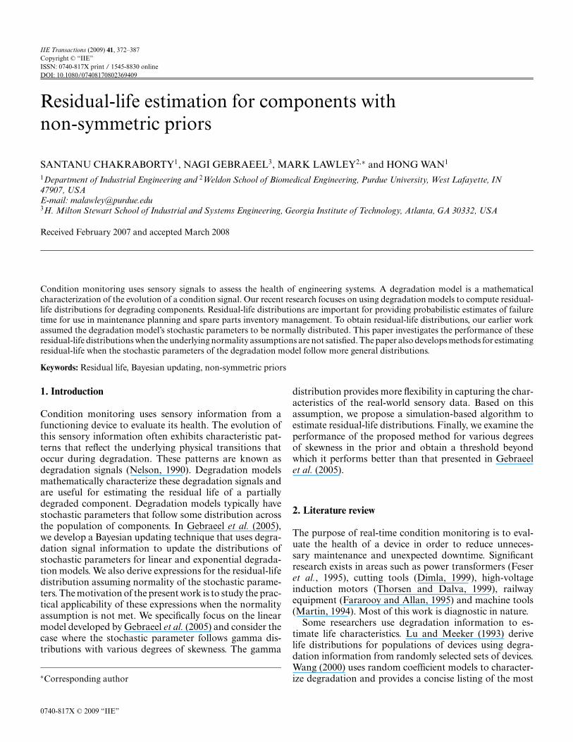
In Gebraeel et al. (2005), we propose a Bayesian tech-nique to update the stochastic parameters for linear andexponential degradation models. Figure 1 shows an exam-ple real-time vibration-based degradation signal for a thrustbearing from Gebraeel (2006). Note that the vibration am-plitude increases with operating time as the bearing de-grades. When the amplitude reaches a pre-specified thresh-

Fig. 1. Example real-time degradation signal from Gebraeel(2006).

old (based on industry standards), the bearing is assumedto fail.

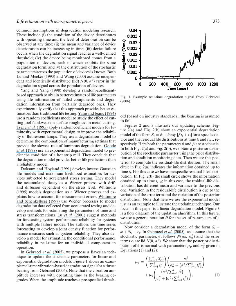
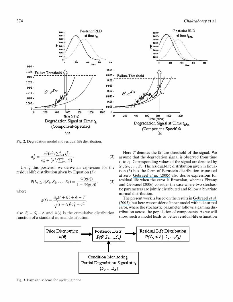
Figures 2 and 3 illustrate our updating scheme. Fig-ure 2(a) and Fig. 2(b) show an exponential degradationmodel of the form Si = φ + θ exp [βti + εi] for a specific de-vice and the residual life distributions at time ti and ti+n, re-spectively. Here both the parameters θ and β are stochastic.In both Fig. 2(a) and Fig. 2(b), we obtain a posterior distri-bution of the stochastic parameter using the prior distribu-tion and condition monitoring data. Then we use this pos-terior to compute the residual-life distribution. The smallcircle in Fig. 2(a) indicates the information obtained up totime ti. For this case we have one specific residual-life distri-bution. In Fig. 2(b) the small circle shows the informationobtained up to time ti+n; in this case, the residual-life dis-tribution has different mean and variance to the previousone. Variation in the residual-life distribution is due to thevariation of the error term and the variation of the posteriordistribution. Note that here we use the exponential modeljust as an example to illustrate the updating technique. Ourfocus in this paper is a linear degradation model. Figure 3is a flow diagram of the updating algorithm. In this figure,we use a generic notation θ for the set of parameters of adistribution.

Now consider a degradation model of the form Si =φ + θ ti + εi. In Gebraeel et al. (2005), we assume that thestochastic parameter, θ , follows N(µ0, σ 2

0 ) and the errorterms εi are iid N(0, σ 2). We show that the posterior distri-bution of θ is normal with parameters µp and σ 2

p given inEquations (1) and (2):

µp =(∑k

i=1 S′iti∑k

i=1 t2i

)(σ 2

0

σ 20 + (

σ 2/∑k

i=1 t2i

))

+ µ0

( (σ 2/

∑ki=1 t2

i

)σ 2

0 + (σ 2/

∑ki=1 t2

i

))

, (1)

374 Chakraborty et al.

Fig. 2. Degradation model and residual life distribution.

σ 2p = σ 2

0

(σ 2/

∑ki=1 t2

i

)σ 2

0 + (σ 2/

∑ki=1 t2

i

) . (2)

Using this posterior we derive an expression for theresidual-life distribution given by Equation (3):

P(Lr ≤ t |S1, S2, . . . , Sk) = �(g(t))1 − �(g(0))

, (3)

where

g(t) = µp(t + tk) + φ − T√(t + tk)2σ 2

p + σ 2,

also S′i = Si − φ and �(·) is the cumulative distribution

function of a standard normal distribution.

Here T denotes the failure threshold of the signal. Weassume that the degradation signal is observed from timet1 to tk. Corresponding values of the signal are denoted byS1, S2, . . . , Sk. The residual-life distribution given in Equa-tion (3) has the form of Bernstein distribution truncatedat zero. Gebraeel et al. (2005) also derive expressions forresidual life when the error is Brownian, whereas Elwanyand Gebraeel (2006) consider the case where two stochas-tic parameters are jointly distributed and follow a bivariatenormal distribution.

The present work is based on the results in Gebraeel et al.(2005); but here we consider a linear model with iid normalerror, where the stochastic parameter follows a gamma dis-tribution across the population of components. As we willshow, such a model leads to better residual-life estimation

Fig. 3. Bayesian scheme for updating prior.

Life estimation with non-symmetric priors 375

when the prior distribution of the stochastic parameter isskewed.

3. Example performance of “normal prior method”

In this section, we illustrate how the truncated Bernstein dis-tribution, given by Equation (3), approximates the residual-life distribution when the prior distribution of the stochasticparameter is skewed. This example will motivate us to de-velop residual-life estimation for skewed priors, which wemodel with the gamma distribution. In this paper, we shallrefer to the method proposed by Gebraeel et al. (2005) asthe “Normal Prior Method.”

Let us consider a family of parts with a degradationmodel of the form Si = θ ti + εi. Here θ is the stochastic co-efficient of the signal and εi, i = 1, 2, . . . are iid error terms.Let T denote the failure threshold of the signal. Note thatthis model does not include the intercept term φ becauseit has no contribution in the posterior distribution. If anintercept is observed in the signal data (Sr

i ), we can use thetransformation Si = Sr

i − φ and apply our algorithm.The Bayesian updating technique in Gebraeel et al. (2005)

requires computing the posterior distribution of θ , given byf (θ |S1, S2, . . . , Sk), using initial observed signal values S1,S2, . . . , Sk. Hence, without loss of generality, we simulatethe signal Si, i = 1, 2 . . . up to half the failure threshold,T/2. Let � = {(S1, S2, . . . , Sn)|Sn+1 > T/2 ≥ Sn}. We referto � as the “Partial Signal.” Let tT/2 denote the time corre-

sponding to Sn in�. We use this “Partial Signal” to computethe posterior distribution as given in Gebraeel et al. (2005).Then we draw random samples from the posterior distribu-tion f (θ |S1, S2, . . . , Sk) and run the signal from time tT/2to the failure threshold T . Let tT denote the time at whichthe signal crosses the failure threshold. The residual-life isgiven by tr = tT − tT/2. We continue simulating from theposterior in this fashion to obtain an empirical residual-lifedistribution. Next, we compare this empirical life distri-bution with the truncated Bernstein of Equation (3). Ourhypothesis is that if the prior distribution has small skew-ness, then the empirical residual-life distribution obtainedfrom simulation will match well with the truncated Bern-stein distribution. However, as we increase the skewness ofthe prior, the residual life approximation obtained from thetruncated Bernstein will deteriorate. We check this usingchi-square goodness of fit tests.

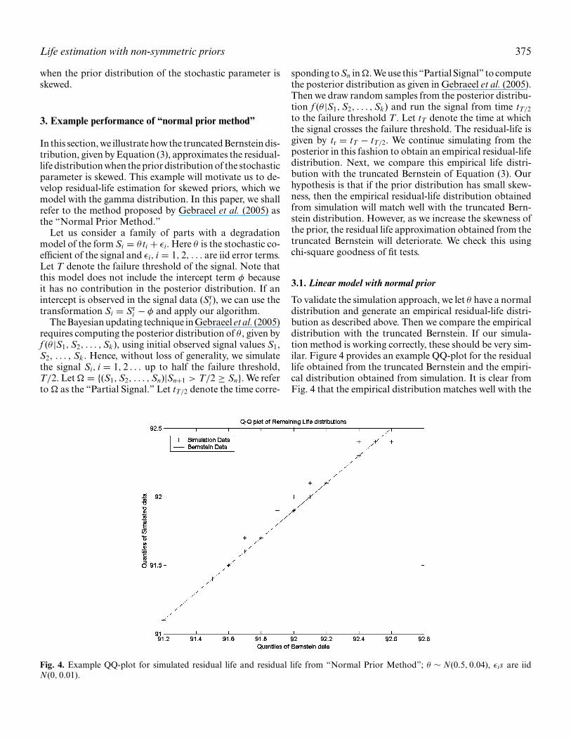
3.1. Linear model with normal prior

To validate the simulation approach, we let θ have a normaldistribution and generate an empirical residual-life distri-bution as described above. Then we compare the empiricaldistribution with the truncated Bernstein. If our simula-tion method is working correctly, these should be very sim-ilar. Figure 4 provides an example QQ-plot for the residuallife obtained from the truncated Bernstein and the empiri-cal distribution obtained from simulation. It is clear fromFig. 4 that the empirical distribution matches well with the

Fig. 4. Example QQ-plot for simulated residual life and residual life from “Normal Prior Method”; θ ∼ N(0.5, 0.04), εis are iidN(0, 0.01).

376 Chakraborty et al.

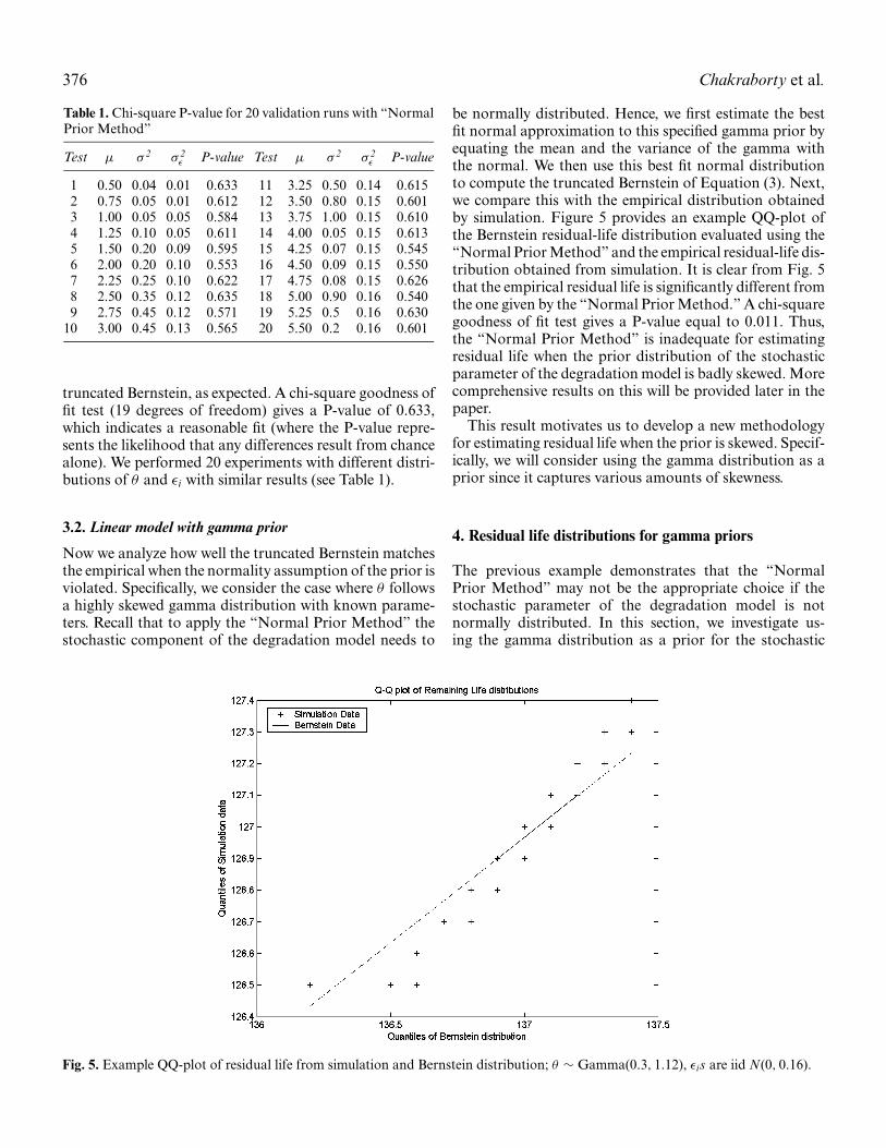
Table 1. Chi-square P-value for 20 validation runs with “NormalPrior Method”

Test µ σ 2 σ 2ε P-value Test µ σ 2 σ 2

ε P-value

1 0.50 0.04 0.01 0.633 11 3.25 0.50 0.14 0.6152 0.75 0.05 0.01 0.612 12 3.50 0.80 0.15 0.6013 1.00 0.05 0.05 0.584 13 3.75 1.00 0.15 0.6104 1.25 0.10 0.05 0.611 14 4.00 0.05 0.15 0.6135 1.50 0.20 0.09 0.595 15 4.25 0.07 0.15 0.5456 2.00 0.20 0.10 0.553 16 4.50 0.09 0.15 0.5507 2.25 0.25 0.10 0.622 17 4.75 0.08 0.15 0.6268 2.50 0.35 0.12 0.635 18 5.00 0.90 0.16 0.5409 2.75 0.45 0.12 0.571 19 5.25 0.5 0.16 0.630

10 3.00 0.45 0.13 0.565 20 5.50 0.2 0.16 0.601

truncated Bernstein, as expected. A chi-square goodness offit test (19 degrees of freedom) gives a P-value of 0.633,which indicates a reasonable fit (where the P-value repre-sents the likelihood that any differences result from chancealone). We performed 20 experiments with different distri-butions of θ and εi with similar results (see Table 1).

3.2. Linear model with gamma prior

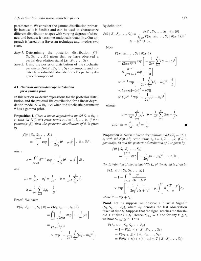
Now we analyze how well the truncated Bernstein matchesthe empirical when the normality assumption of the prior isviolated. Specifically, we consider the case where θ followsa highly skewed gamma distribution with known parame-ters. Recall that to apply the “Normal Prior Method” thestochastic component of the degradation model needs to

be normally distributed. Hence, we first estimate the bestfit normal approximation to this specified gamma prior byequating the mean and the variance of the gamma withthe normal. We then use this best fit normal distributionto compute the truncated Bernstein of Equation (3). Next,we compare this with the empirical distribution obtainedby simulation. Figure 5 provides an example QQ-plot ofthe Bernstein residual-life distribution evaluated using the“Normal Prior Method” and the empirical residual-life dis-tribution obtained from simulation. It is clear from Fig. 5that the empirical residual life is significantly different fromthe one given by the “Normal Prior Method.” A chi-squaregoodness of fit test gives a P-value equal to 0.011. Thus,the “Normal Prior Method” is inadequate for estimatingresidual life when the prior distribution of the stochasticparameter of the degradation model is badly skewed. Morecomprehensive results on this will be provided later in thepaper.

This result motivates us to develop a new methodologyfor estimating residual life when the prior is skewed. Specif-ically, we will consider using the gamma distribution as aprior since it captures various amounts of skewness.

4. Residual life distributions for gamma priors

The previous example demonstrates that the “NormalPrior Method” may not be the appropriate choice if thestochastic parameter of the degradation model is notnormally distributed. In this section, we investigate us-ing the gamma distribution as a prior for the stochastic

Fig. 5. Example QQ-plot of residual life from simulation and Bernstein distribution; θ ∼ Gamma(0.3, 1.12), εis are iid N(0, 0.16).

Life estimation with non-symmetric priors 377

parameter θ . We consider the gamma distribution primar-ily because it is flexible and can be used to characterizedifferent distribution shapes with varying degrees of skew-ness and because it has some analytical tractability. Our ap-proach is based on a Bayesian technique and involves twosteps.

Step 1. Determining the posterior distribution f (θ |S1, S2, . . . , Sk) given that we have observed apartial degradation signal (S1, S2, . . . , Sk).

Step 2. Using the posterior distribution of the stochasticparameter f (θ |S1, S2, . . . , Sk) to compute and up-date the residual-life distribution of a partially de-graded component.

4.1. Posterior and residual life distributionfor a gamma prior

In this section we derive expressions for the posterior distri-bution and the residual-life distribution for a linear degra-dation model Si = θ ti + εi when the stochastic parameterθ has a gamma prior.

Proposition 1. Given a linear degradation model Si = θ ti +εi with iid N(0, σ 2) error terms εi, i = 1, 2, . . . , k, if θ ∼gamma(α, β), then the posterior distribution of θ is givenby

f (θ | S1, S2, . . . , Sk)

= θα−1

cexp

[− 1

2σ 21

(θ − µ1)2]

, θ ∈ R+ ,

where

c =∫ ∞

θ=0θα−1 exp

[− 1

2σ 21

(θ − µ1)2]

dθ ,

and

µ1 = b2a

, σ 21 = 1

2a, a = 1

2σ 2

k∑i=1

t2i ,

b = 1σ 2

k∑i=1

Siti − 1β

.

Proof. We have:

P(S1, S2, . . . , Sk | θ ) = P(ε1, ε2, . . . , εk | θ )

=k∏

i=1

1√2πσ

exp[

− 12σ 2

ε2i

]

= 1(2πσ 2)k/2

× exp[

− 12σ 2

k∑i=1

(Si − θ ti)2]

.

By definition

P(θ | S1, S2, . . . , Sk) = P(S1, S2, . . . , Sk | θ )π (θ )∫θ∈

P(S1, S2, . . . , Sk | θ )π (θ )dθ,

= R+ ∪ {0} .

Now

P(S1, S2, . . . , Sk | θ )π (θ )

= 1(2πσ 2)k/2

exp[

− 12σ 2

k∑i=1

(Si − θti)2]

× θα−1

βα�(α)exp

[− θ

β

]

∝ θα−1 exp[

− 12σ 2

k∑i=1

(Si − θ ti)2 − θ

β

]

∝ C2 exp[−(aθ2 − bθ )]

∝ C3θα−1 exp

[− 1

2σ 21

(θ − µ1)2]

,

where,

a = 12σ 2

k∑i=1

t2i , b = 1

σ 2

k∑i=1

Siti − 1β

,

and µ1 = b2a

, σ 21 = 1

2a �

Proposition 2. Given a linear degradation model Si = θ ti +εi with iid N(0, σ 2) error terms εi, i = 1, 2, . . . , k, if θ ∼gamma(α, β) and the posterior distribution of θ is given by

f (θ | S1, S2, . . . , Sk)

= θα−1

cexp

[− 1

2σ 21

(θ − µ1)2], θ ∈ R

+,

the distribution of the residual-life Lr of the signal is given by

P(Lr ≤ t | S1, S2, . . . , Sk)

= 1 −∫ +∞

y=0

yα−1

c(t + tk)α

× exp

[− 1

2σ 21

(y

(t + tk)− µ1

)2]�

(T − y

σ

)dy

where Y = θ (t + tk).

Proof. Let us suppose we observe a “Partial Signal”(S1, S2, . . . , Sk), where Sk denotes the last observationtaken at time tk. Suppose that the signal reaches the thresh-old T at time t + tk. Hence, St+tk = T and for any t ′ ≤ t ,we have St ′+tk ≤ T . Thus

P(Lr > t | S1, S2, . . . , Sk)= 1 − P(Lr ≤ t | S1, S2, . . . , Sk)= P(St+tk ≤ T | S1, S2, . . . , Sk)= P(θ (t + tk) + ε(t + tk) ≤ T | S1, S2, . . . , Sk).

378 Chakraborty et al.

Let us put Y = θ (t + tk) ∈ R+ and let f1(y) be the proba-

bility distribution of Y . Then

f1(y) = yα−1

c(t + tk)α−1exp

[− 1

2σ 21

(y

(t + tk)− µ1

)2] ∣∣∣∣dθ

dy

∣∣∣∣= yα−1

c(t + tk)αexp

[− 1

2σ 21

(y

(t + tk)− µ1

)2].

Now let U = Y + ε. Let g(., .) be the joint distribution ofY and ε. Let φ(.) be the probability distribution function ofε, then g(y, ε) = f1(y)φ(ε), since Y and ε are independent.Hence

P(U ≤ u) = P(Y + ε ≤ u)

=∫ +∞

y=0

∫ u−y

ε=−∞g(y, ε)dydε

=∫ +∞

y=0

∫ u−y

ε=−∞f1(y)φ(ε)dydε

=∫ +∞

y=0

∫ u−y

ε=−∞

yα−1

c(t + tk)α

× exp

[− 1

2σ 21

(y

(t + tk)− µ1

)2]

× 1√2πσ

exp[− ε2

2σ 2

]dydε

=∫ +∞

y=0

yα−1

c(t + tk)α

× exp

[− 1

2σ 21

(y

(t + tk)− µ1

)2]

dy

×∫ u−y

ε=−∞

1√2πσ

exp[− ε2

2σ 2

]dε

=∫ +∞

y=0

yα−1

c(t + tk)α

× exp

[− 1

2σ 21

(y

(t + tk)− µ1

)2]

× �

(u − y

σ

)dy.

Hence

P(Lr > t | S1, S2, . . . , Sk)= P(θ (t + tk) + ε(t + tk) ≤ T | S1, S2, . . . , Sk)= P(U ≤ T)

=∫ +∞

y=0

yα−1

c(t + tk)αexp

[− 1

2σ 21

(y

(t + tk)− µ1

)2]

× �

(T − y

σ

)dy.

Therefore

P(Lr ≤ t | S1, S2, . . . , Sk)= 1 − P(Lr > t | S1, S2, . . . , Sk)

= 1 −∫ +∞

y=0

yα−1

c(t + tk)αexp

[− 1

2σ 21

(y

(t + tk)− µ1

)2]

× �

(T − y

σ

)dy

�

Note that in Proposition 1, c is the normalizing constantfor the posterior distribution of θ . To our knowledge, thereis no closed form, hence we use numerical integration. Theintegrand is a simple function and any standard computingpackage with built-in procedure for numerical integrationcan solve it easily. Note that for a given prior distribu-tion we need to calculate c once each time the posterior isupdated.

Proposition 2 expresses the residual life distribution ofthe signal in the form of a integration involving the cumu-lative distribution function � of the standard normal dis-tribution. Hence, to calculate the probability of the residuallife at any point, t , we must use numerical integration. Inthis case, however, the integrand is a rather complicatedfunction, and we need to use fine intervals to evaluate itnumerically. This results in slower evaluation times, and wehave not yet been successful in doing this quickly. Further-more, to get the distribution of residual life, the functionmust be evaluated at many points over its entire support.So we have to do the numerical integration for a fairly largenumber of points. Hence, in this work we develop an al-ternative technique for getting the residual-life distributiononce the posterior is known, and we leave the numericalintegration problem for future research.

4.2. Empirical residual life distribution for a gamma prior

Given the posterior distribution of the stochastic parame-ter for a linear degradation model, we develop a simulation-based approach to compute an empirical residual life dis-tribution. We refer to this new technique as the “GammaPrior Method.”

Our objective is to generate the residual life distributionof a component using the prior distribution of its stochasticparameter and data from its “Partial Signal.” Hence, given a“Partial Signal”, we first compute the posterior distributionf (θ | S1, S2, . . . , Sk) using �. Then we make random drawsfrom this posterior and, for each draw, run the signal fromtime tT/2 to failure. Thus, each draw from the posterior gen-erates residual life value, tr = tT − tT/2 (c.f. Section 3). Thecollection of these residual-life values provides an empiri-cal distribution for the given “Partial Signal.” Algorithm 1illustrates the technique.

Life estimation with non-symmetric priors 379

Algorithm 1. Methods to construct empirical residual-life distribution

Input: Prior ∼ �(θ | µ), Error ε ∼N(0, σ 2), Threshold TOutput: Set of Empirical Residual livesforeach Signal i do

Generate θ∗i from �(θ |µ)

foreach Value j doGenerate Signal S∗(i, j) = φ + θ∗

i tj + εj;if S∗(i, j) ≥ T/2 then hit timei = j; break;

endSet S obs = {S∗(i, 1), S∗(i, 2), . . . , S∗(i, hit timei)};Calculate parameters of f (θ | S∗(i, 1), S∗(i, 2), . . . , S∗(i, hit timei)) using S obs;foreach m do

Generate θpij m from posterior distribution f (θ | S(i, 1), S(i, 2), . . . , S(i, hit timei));

foreach Value k do

Generate Signal Sp(i, m, k) = φ + θpimtk + εk;

if Sp(i, m, k) ≥ T then post hit timeim = k; break;

endSet R lif e(i, m) = post hit timeim − hit timei;

endend

Note that there is no standard method to generate ran-dom variates from the posterior distribution derived above(c.f. Proposition 1). Hence, we use the Metropolis–Hasting(Metropolis et al., 1953; Hasting, 1970; Tierney, 1994;Chib and Greenberg, 1995) algorithm to sample from it.We provide a brief review of the Metropolis–Hastingsalgorithm in Algorithm 2.

4.2.1. Review of Metropolis–Hastings algorithmSuppose we want to draw random samples from a dis-tribution π (x). One approach is to generate a sequence{Xn} from a Markov chain with steady-state distribu-tion π (.). The Metropolis–Hastings algorithm can be usedto generate such a Markov chain for any given distri-bution π (.) provided we can calculate the density at the

Algorithm 2. Metropolis–Hastings algorithm

Input: Proposal distribution q(y | x), initial value x0 from the support of target distribution π

Output: Markov chain with stationary distribution π

foreach Value n do

Generate y from proposal distribution q(y; xn);Set ρ(xn, y) = q(xn; y)π (y)/q(y; xn)π (xn);if q(y; xn)π (xn) > 0 then

Set α(xn, y) = min{ρ(xn, y), 1};endelse

Set α(xn, y) = 0;endDraw u from U(0, 1);if u ≤ α(xn, y) then

Set xn+1 = y;

endelse

Set xn+1 = xn;

endend

380 Chakraborty et al.

point x. Hence, we need to know π (x) up to the normalizingconstant.

Let us select an arbitrary distribution q(y; x) = q(y | x)as our proposal distribution. Here q(y; x) represents thesingle-step transition probability from state x to state y. Theinitial algorithm proposed by Metropolis requires the pro-posal distribution to be symmetric, i.e., q(y; x) = q(x; y).Later Hastings relaxed this condition. We start the itera-tion with an initial value x0 from the support of the targetdistribution π (x). At the nth state, we draw a new pro-posal state y with probability q(y; xn). Next we calculatethe expression ρ(xn, y) = ρ1ρ2, where ρ1 = π (y)/π (xn) andρ2 = q(xn; y)/q(y; xn). Note that ρ1 is the likelihood ratioof the proposed state y and the current state xn and ρ2 is theratio of probabilities of jumping from state y to state xn. Ifthe proposal distribution is symmetric, we have ρ2 = 1. Let

α(xn, y) ={

min {ρ(xn, y), 1} if π (xn)q(y; xn) > 0,

1 otherwise.

Let u be a random draw from uniform (0, 1). Now to selectthe next state xn+1, we use the following rule:

xn+1 ={

y if u ≤ α(xn, y),

xn otherwise.

The distribution of the chain {Xn}n≥1 converges to π asn → ∞. Thus, it is customary to leave out a certain numbervalues, say n0, at the start of the sequence {Xn}n≥1 and usethe subsequent draws as the random samples from π . Thesamples {Xn}n0

n=1 are called burn-in.

5. Comparing “gamma prior” and “normal prior”

In this section, we present a comparative study of the ap-proximations provided by the “Normal Prior Method” andthe “Gamma Prior Method” for different types of priors.We test both methods using two scenarios. First, we con-sider the case when the stochastic parameter θ of the lineardegradation model follows a symmetric prior. Second, wetest the case where θ has a skewed prior distribution. Finally,we evaluate the behavior of these two methods at differentdegrees of skewness of the distribution of θ .

5.1. Study for symmetric prior distributions of θ

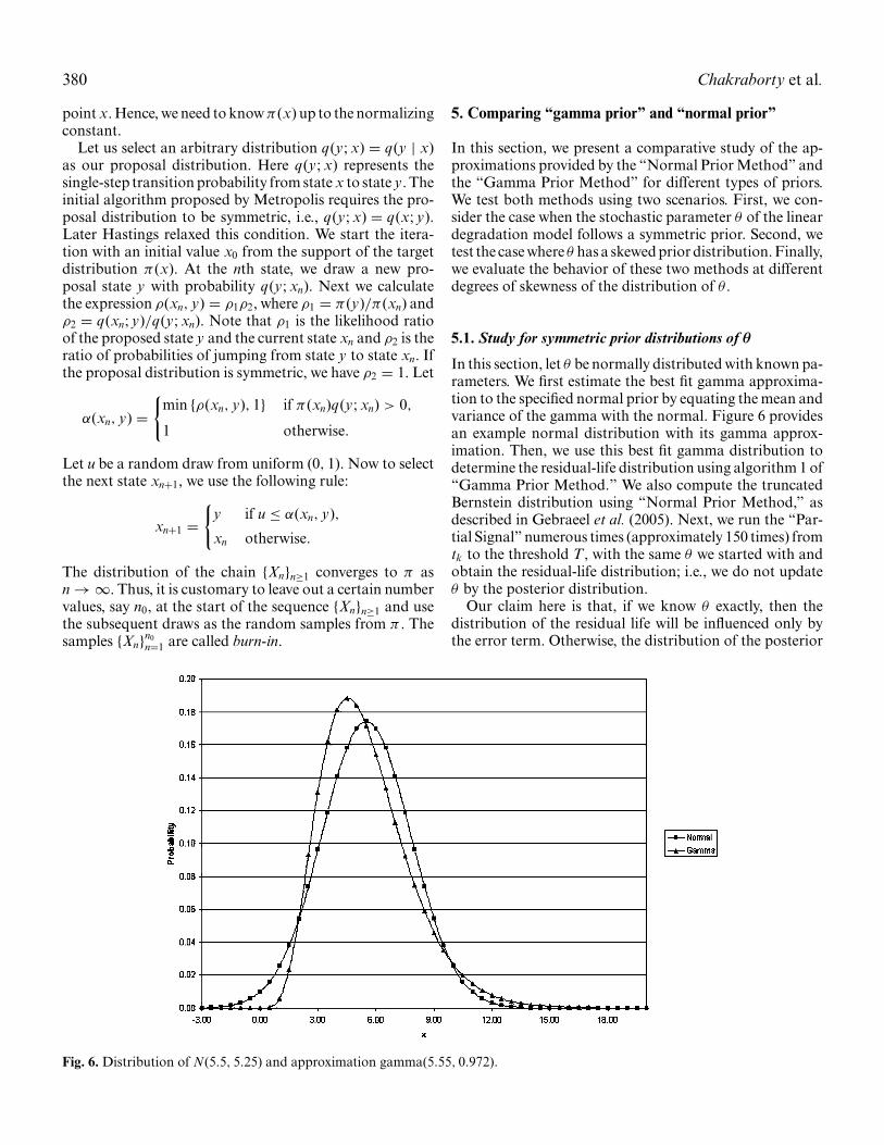
In this section, let θ be normally distributed with known pa-rameters. We first estimate the best fit gamma approxima-tion to the specified normal prior by equating the mean andvariance of the gamma with the normal. Figure 6 providesan example normal distribution with its gamma approx-imation. Then, we use this best fit gamma distribution todetermine the residual-life distribution using algorithm 1 of“Gamma Prior Method.” We also compute the truncatedBernstein distribution using “Normal Prior Method,” asdescribed in Gebraeel et al. (2005). Next, we run the “Par-tial Signal” numerous times (approximately 150 times) fromtk to the threshold T , with the same θ we started with andobtain the residual-life distribution; i.e., we do not updateθ by the posterior distribution.

Our claim here is that, if we know θ exactly, then thedistribution of the residual life will be influenced only bythe error term. Otherwise, the distribution of the posterior

Fig. 6. Distribution of N(5.5, 5.25) and approximation gamma(5.55, 0.972).

Life estimation with non-symmetric priors 381

Fig. 7. Histogram of residual lives from “Gamma Prior Method”, “Normal Prior Method” and “Partial Signal” for normal prior.

plays a major role. However, if it is possible to reduce thevariance of the posterior to a great extent, we can practicallyconsider that θ is known. Now if we compute the posteriorbased on a large number of observations, we can reduceits variance. Recall that we are estimating the posterior at apoint where the signal has reached half the failure threshold.We divided this time horizon in such a fashion that there areon average 200 observations in the interval. Table 2 providesa comparison the variances of the posterior and the errorterms. Here σ 2

ε and σ 2P denotes the variance of the error

and the posterior respectively. Note that the ratio σ 2ε /σ 2

P isalways very high. Thus, we can conclude that in these casesthe effect of the posterior on the residual-life is very smallin comparison to the error.

Table 2. Comparison of variance of error and variance of theposterior

Skewness σ 2ε σ 2

P σ 2ε /σ 2

P

5.16 0.16 1 × 10−3 145.453.65 0.18 8 × 10−4 202.232.39 0.20 9 × 10−4 210.522.00 0.15 8 × 10−4 180.721.63 0.17 8 × 10−4 200.001.26 0.19 1 × 10−3 190.001.15 0.15 8 × 10−4 168.54

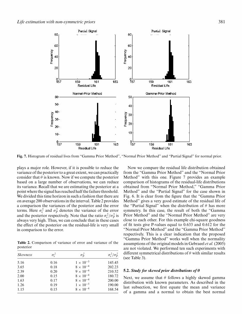
Now we compare the residual life distribution obtainedfrom the “Gamma Prior Method” and the “Normal PriorMethod” with this one. Figure 7 provides an examplecomparison of histograms of the residual-life distributionsobtained from “Normal Prior Method,” “Gamma PriorMethod” and the “Partial Signal” for the case shown inFig. 6. It is clear from the figure that the “Gamma PriorMethod” gives a very good estimate of the residual life ofthe “Partial Signal” when the distribution of θ has moresymmetry. In this case, the result of both the “GammaPrior Method” and the “Normal Prior Method” are veryclose to each other. For this example chi-square goodnessof fit tests give P-values equal to 0.633 and 0.612 for the“Normal Prior Method” and the “Gamma Prior Method”respectively. This is a clear indication that the proposed“Gamma Prior Method” works well when the normalityassumptions of the original models in Gebraeel et al. (2005)are not violated. We performed ten such experiments withdifferent symmetrical distributions of θ with similar results(see Table 3).

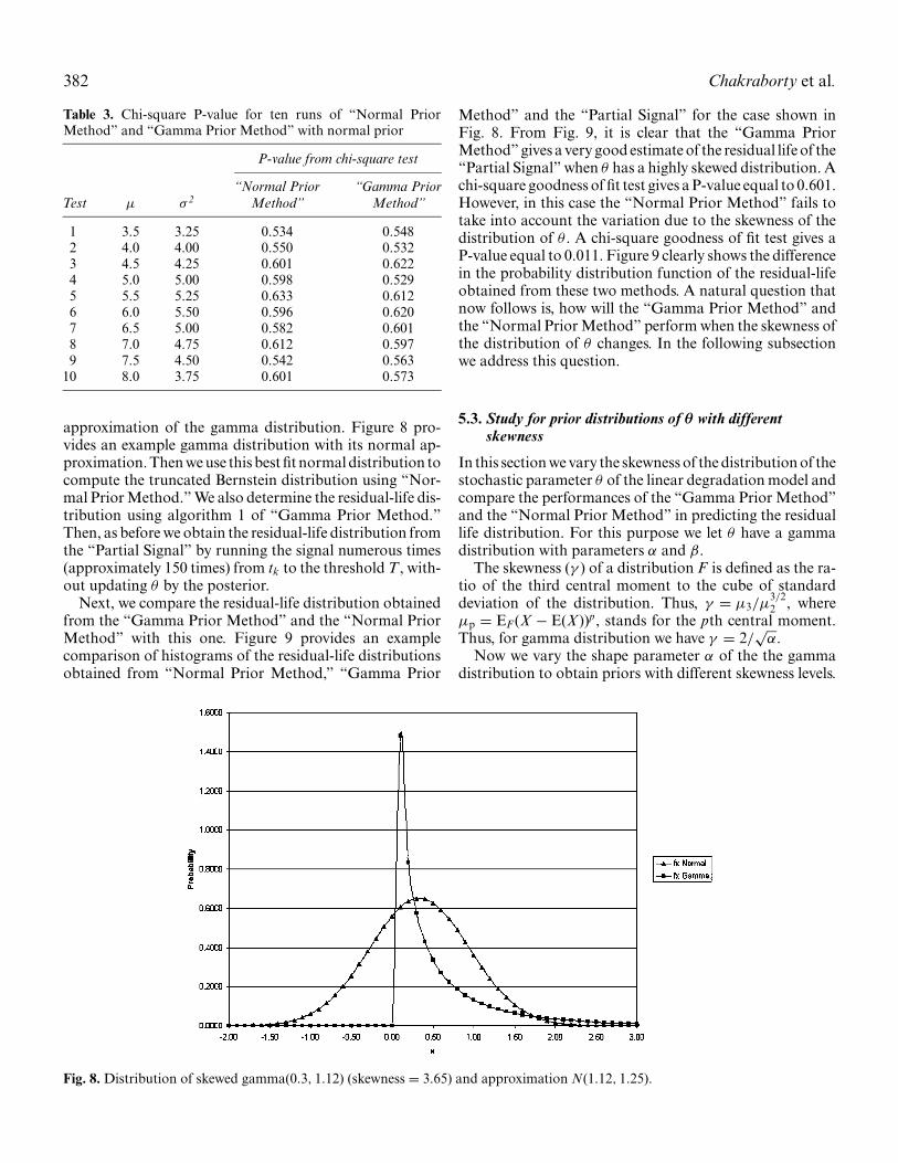
5.2. Study for skewed prior distributions of θ

Next, we assume that θ follows a highly skewed gammadistribution with known parameters. As described in thelast subsection, we first equate the mean and varianceof a gamma and a normal to obtain the best normal

382 Chakraborty et al.

Table 3. Chi-square P-value for ten runs of “Normal PriorMethod” and “Gamma Prior Method” with normal prior

P-value from chi-square test

“Normal Prior “Gamma PriorTest µ σ 2 Method” Method”

1 3.5 3.25 0.534 0.5482 4.0 4.00 0.550 0.5323 4.5 4.25 0.601 0.6224 5.0 5.00 0.598 0.5295 5.5 5.25 0.633 0.6126 6.0 5.50 0.596 0.6207 6.5 5.00 0.582 0.6018 7.0 4.75 0.612 0.5979 7.5 4.50 0.542 0.563

10 8.0 3.75 0.601 0.573

approximation of the gamma distribution. Figure 8 pro-vides an example gamma distribution with its normal ap-proximation. Then we use this best fit normal distribution tocompute the truncated Bernstein distribution using “Nor-mal Prior Method.” We also determine the residual-life dis-tribution using algorithm 1 of “Gamma Prior Method.”Then, as before we obtain the residual-life distribution fromthe “Partial Signal” by running the signal numerous times(approximately 150 times) from tk to the threshold T , with-out updating θ by the posterior.

Next, we compare the residual-life distribution obtainedfrom the “Gamma Prior Method” and the “Normal PriorMethod” with this one. Figure 9 provides an examplecomparison of histograms of the residual-life distributionsobtained from “Normal Prior Method,” “Gamma Prior

Method” and the “Partial Signal” for the case shown inFig. 8. From Fig. 9, it is clear that the “Gamma PriorMethod” gives a very good estimate of the residual life of the“Partial Signal” when θ has a highly skewed distribution. Achi-square goodness of fit test gives a P-value equal to 0.601.However, in this case the “Normal Prior Method” fails totake into account the variation due to the skewness of thedistribution of θ . A chi-square goodness of fit test gives aP-value equal to 0.011. Figure 9 clearly shows the differencein the probability distribution function of the residual-lifeobtained from these two methods. A natural question thatnow follows is, how will the “Gamma Prior Method” andthe “Normal Prior Method” perform when the skewness ofthe distribution of θ changes. In the following subsectionwe address this question.

5.3. Study for prior distributions of θ with differentskewness

In this section we vary the skewness of the distribution of thestochastic parameter θ of the linear degradation model andcompare the performances of the “Gamma Prior Method”and the “Normal Prior Method” in predicting the residuallife distribution. For this purpose we let θ have a gammadistribution with parameters α and β.

The skewness (γ ) of a distribution F is defined as the ra-tio of the third central moment to the cube of standarddeviation of the distribution. Thus, γ = µ3/µ

3/22 , where

µp = EF (X − E(X))p, stands for the pth central moment.Thus, for gamma distribution we have γ = 2/

√α.

Now we vary the shape parameter α of the the gammadistribution to obtain priors with different skewness levels.

Fig. 8. Distribution of skewed gamma(0.3, 1.12) (skewness = 3.65) and approximation N(1.12, 1.25).

Life estimation with non-symmetric priors 383

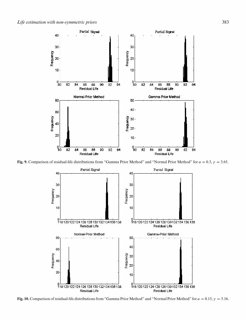
Fig. 9. Comparison of residual-life distributions from “Gamma Prior Method” and “Normal Prior Method” for α = 0.3, γ = 3.65.

Fig. 10. Comparison of residual-life distributions from “Gamma Prior Method” and “Normal Prior Method” for α = 0.15, γ = 5.16.

384 Chakraborty et al.

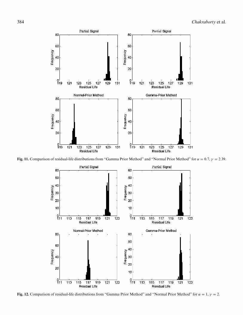
Fig. 11. Comparison of residual-life distributions from “Gamma Prior Method” and “Normal Prior Method” for α = 0.7, γ = 2.39.

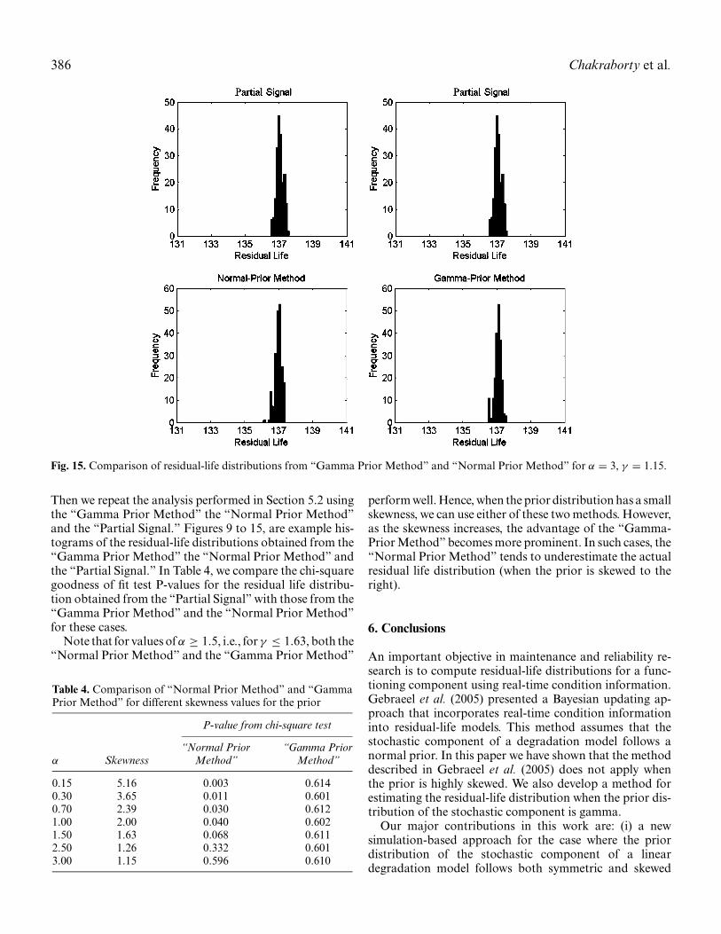
Fig. 12. Comparison of residual-life distributions from “Gamma Prior Method” and “Normal Prior Method” for α = 1, γ = 2.

Life estimation with non-symmetric priors 385

Fig. 13. Comparison of residual-life distributions from “Gamma Prior Method” and “Normal Prior Method” for α = 1.5, γ = 1.63.

Fig. 14. Comparison of residual-life distributions from “Gamma Prior Method” and “Normal Prior Method” for α = 2.5, γ = 1.26.

386 Chakraborty et al.

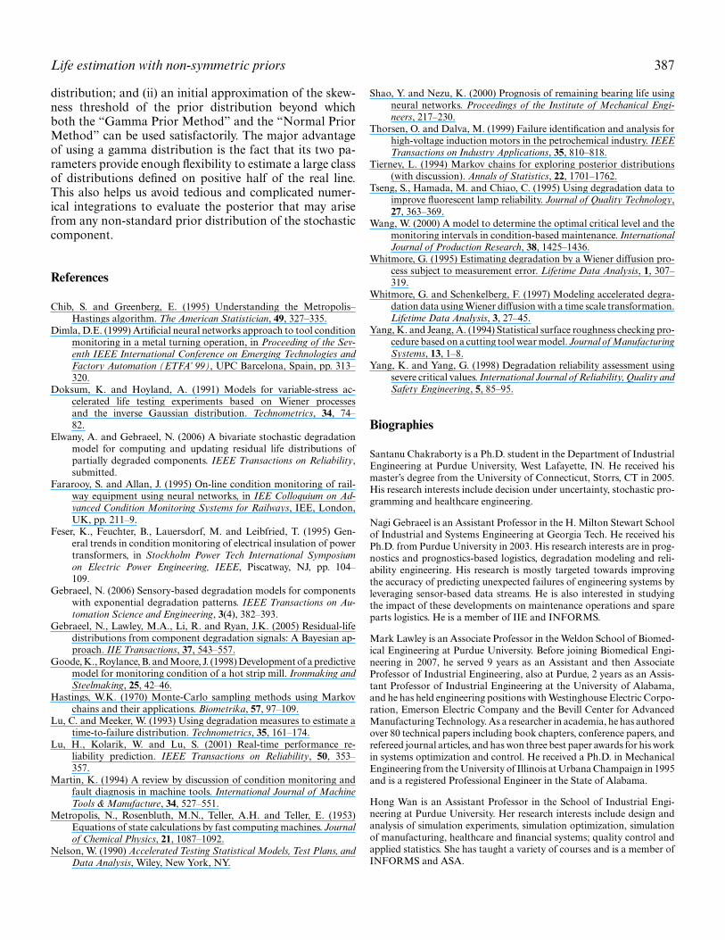
Fig. 15. Comparison of residual-life distributions from “Gamma Prior Method” and “Normal Prior Method” for α = 3, γ = 1.15.

Then we repeat the analysis performed in Section 5.2 usingthe “Gamma Prior Method” the “Normal Prior Method”and the “Partial Signal.” Figures 9 to 15, are example his-tograms of the residual-life distributions obtained from the“Gamma Prior Method” the “Normal Prior Method” andthe “Partial Signal.” In Table 4, we compare the chi-squaregoodness of fit test P-values for the residual life distribu-tion obtained from the “Partial Signal” with those from the“Gamma Prior Method” and the “Normal Prior Method”for these cases.

Note that for values of α ≥ 1.5, i.e., for γ ≤ 1.63, both the“Normal Prior Method” and the “Gamma Prior Method”

Table 4. Comparison of “Normal Prior Method” and “GammaPrior Method” for different skewness values for the prior

P-value from chi-square test

“Normal Prior “Gamma Priorα Skewness Method” Method”

0.15 5.16 0.003 0.6140.30 3.65 0.011 0.6010.70 2.39 0.030 0.6121.00 2.00 0.040 0.6021.50 1.63 0.068 0.6112.50 1.26 0.332 0.6013.00 1.15 0.596 0.610

perform well. Hence, when the prior distribution has a smallskewness, we can use either of these two methods. However,as the skewness increases, the advantage of the “Gamma-Prior Method” becomes more prominent. In such cases, the“Normal Prior Method” tends to underestimate the actualresidual life distribution (when the prior is skewed to theright).

6. Conclusions

An important objective in maintenance and reliability re-search is to compute residual-life distributions for a func-tioning component using real-time condition information.Gebraeel et al. (2005) presented a Bayesian updating ap-proach that incorporates real-time condition informationinto residual-life models. This method assumes that thestochastic component of a degradation model follows anormal prior. In this paper we have shown that the methoddescribed in Gebraeel et al. (2005) does not apply whenthe prior is highly skewed. We also develop a method forestimating the residual-life distribution when the prior dis-tribution of the stochastic component is gamma.

Our major contributions in this work are: (i) a newsimulation-based approach for the case where the priordistribution of the stochastic component of a lineardegradation model follows both symmetric and skewed

Life estimation with non-symmetric priors 387

distribution; and (ii) an initial approximation of the skew-ness threshold of the prior distribution beyond whichboth the “Gamma Prior Method” and the “Normal PriorMethod” can be used satisfactorily. The major advantageof using a gamma distribution is the fact that its two pa-rameters provide enough flexibility to estimate a large classof distributions defined on positive half of the real line.This also helps us avoid tedious and complicated numer-ical integrations to evaluate the posterior that may arisefrom any non-standard prior distribution of the stochasticcomponent.

References

Chib, S. and Greenberg, E. (1995) Understanding the Metropolis–Hastings algorithm. The American Statistician, 49, 327–335.

Dimla, D.E. (1999) Artificial neural networks approach to tool conditionmonitoring in a metal turning operation, in Proceeding of the Sev-enth IEEE International Conference on Emerging Technologies andFactory Automation (ETFA’ 99), UPC Barcelona, Spain, pp. 313–320.

Doksum, K. and Hoyland, A. (1991) Models for variable-stress ac-celerated life testing experiments based on Wiener processesand the inverse Gaussian distribution. Technometrics, 34, 74–82.

Elwany, A. and Gebraeel, N. (2006) A bivariate stochastic degradationmodel for computing and updating residual life distributions ofpartially degraded components. IEEE Transactions on Reliability,submitted.

Fararooy, S. and Allan, J. (1995) On-line condition monitoring of rail-way equipment using neural networks, in IEE Colloquium on Ad-vanced Condition Monitoring Systems for Railways, IEE, London,UK, pp. 211–9.

Feser, K., Feuchter, B., Lauersdorf, M. and Leibfried, T. (1995) Gen-eral trends in condition monitoring of electrical insulation of powertransformers, in Stockholm Power Tech International Symposiumon Electric Power Engineering, IEEE, Piscatway, NJ, pp. 104–109.

Gebraeel, N. (2006) Sensory-based degradation models for componentswith exponential degradation patterns. IEEE Transactions on Au-tomation Science and Engineering, 3(4), 382–393.

Gebraeel, N., Lawley, M.A., Li, R. and Ryan, J.K. (2005) Residual-lifedistributions from component degradation signals: A Bayesian ap-proach. IIE Transactions, 37, 543–557.

Goode, K., Roylance, B. and Moore, J. (1998) Development of a predictivemodel for monitoring condition of a hot strip mill. Ironmaking andSteelmaking, 25, 42–46.

Hastings, W.K. (1970) Monte-Carlo sampling methods using Markovchains and their applications. Biometrika, 57, 97–109.

Lu, C. and Meeker, W. (1993) Using degradation measures to estimate atime-to-failure distribution. Technometrics, 35, 161–174.

Lu, H., Kolarik, W. and Lu, S. (2001) Real-time performance re-liability prediction. IEEE Transactions on Reliability, 50, 353–357.

Martin, K. (1994) A review by discussion of condition monitoring andfault diagnosis in machine tools. International Journal of MachineTools & Manufacture, 34, 527–551.

Metropolis, N., Rosenbluth, M.N., Teller, A.H. and Teller, E. (1953)Equations of state calculations by fast computing machines. Journalof Chemical Physics, 21, 1087–1092.

Nelson, W. (1990) Accelerated Testing Statistical Models, Test Plans, andData Analysis, Wiley, New York, NY.

Shao, Y. and Nezu, K. (2000) Prognosis of remaining bearing life usingneural networks. Proceedings of the Institute of Mechanical Engi-neers, 217–230.

Thorsen, O. and Dalva, M. (1999) Failure identification and analysis forhigh-voltage induction motors in the petrochemical industry. IEEETransactions on Industry Applications, 35, 810–818.

Tierney, L. (1994) Markov chains for exploring posterior distributions(with discussion). Annals of Statistics, 22, 1701–1762.

Tseng, S., Hamada, M. and Chiao, C. (1995) Using degradation data toimprove fluorescent lamp reliability. Journal of Quality Technology,27, 363–369.

Wang, W. (2000) A model to determine the optimal critical level and themonitoring intervals in condition-based maintenance. InternationalJournal of Production Research, 38, 1425–1436.

Whitmore, G. (1995) Estimating degradation by a Wiener diffusion pro-cess subject to measurement error. Lifetime Data Analysis, 1, 307–319.

Whitmore, G. and Schenkelberg, F. (1997) Modeling accelerated degra-dation data using Wiener diffusion with a time scale transformation.Lifetime Data Analysis, 3, 27–45.

Yang, K. and Jeang, A. (1994) Statistical surface roughness checking pro-cedure based on a cutting tool wear model. Journal of ManufacturingSystems, 13, 1–8.

Yang, K. and Yang, G. (1998) Degradation reliability assessment usingsevere critical values. International Journal of Reliability, Quality andSafety Engineering, 5, 85–95.

Biographies

Santanu Chakraborty is a Ph.D. student in the Department of IndustrialEngineering at Purdue University, West Lafayette, IN. He received hismaster’s degree from the University of Connecticut, Storrs, CT in 2005.His research interests include decision under uncertainty, stochastic pro-gramming and healthcare engineering.

Nagi Gebraeel is an Assistant Professor in the H. Milton Stewart Schoolof Industrial and Systems Engineering at Georgia Tech. He received hisPh.D. from Purdue University in 2003. His research interests are in prog-nostics and prognostics-based logistics, degradation modeling and reli-ability engineering. His research is mostly targeted towards improvingthe accuracy of predicting unexpected failures of engineering systems byleveraging sensor-based data streams. He is also interested in studyingthe impact of these developments on maintenance operations and spareparts logistics. He is a member of IIE and INFORMS.

Mark Lawley is an Associate Professor in the Weldon School of Biomed-ical Engineering at Purdue University. Before joining Biomedical Engi-neering in 2007, he served 9 years as an Assistant and then AssociateProfessor of Industrial Engineering, also at Purdue, 2 years as an Assis-tant Professor of Industrial Engineering at the University of Alabama,and he has held engineering positions with Westinghouse Electric Corpo-ration, Emerson Electric Company and the Bevill Center for AdvancedManufacturing Technology. As a researcher in academia, he has authoredover 80 technical papers including book chapters, conference papers, andrefereed journal articles, and has won three best paper awards for his workin systems optimization and control. He received a Ph.D. in MechanicalEngineering from the University of Illinois at Urbana Champaign in 1995and is a registered Professional Engineer in the State of Alabama.

Hong Wan is an Assistant Professor in the School of Industrial Engi-neering at Purdue University. Her research interests include design andanalysis of simulation experiments, simulation optimization, simulationof manufacturing, healthcare and financial systems; quality control andapplied statistics. She has taught a variety of courses and is a member ofINFORMS and ASA.