Structural Gaussian Priors for Bayesian CT

reconstruction of Subsea Pipes

Silja W. Christensen, Nicolai A. B. Riis, Felipe Uribe, and Jakob S.Jørgensen

Department of Applied Mathematics and Computer Science, Technical University of Denmark,Kongens Lyngby, Denmark

E-mail: swech@dtu.dk

Abstract. A non-destructive testing (NDT) application of X-ray computed tomography (CT)is inspection of subsea pipes in operation via 2D cross-sectional scans. Data acquisition is time-consuming and costly due to the challenging subsea environment. Reducing the number ofprojections in a scan can yield time and cost savings, but compromises the reconstructionquality, if conventional reconstruction methods are used. In this work we take a Bayesianapproach to CT reconstruction and focus on designing an effective prior to make use of availablestructural information about the pipe geometry. We propose a new class of structural Gaussianpriors to enforce expected material properties in different regions of the reconstructed imagebased on independent Gaussian priors in combination with global regularity through a GaussianMarkov Random Field (GMRF) prior. Numerical experiments with synthetic and real data showthat the proposed structural Gaussian prior can reduce artifacts and enhance contrast in thereconstruction compared to using only a global GMRF prior or no prior at all. We show howthe resulting posterior distribution can be efficiently sampled even for large-scale images, whichis essential for practical NDT applications.

1. IntroductionSubsea pipelines are used to transport oil and gas around the world. It is crucial that thesubsea pipes are in good condition to avoid environmentally damaging leaks. Therefore, efficientmethods for non-destructive inspection are in demand. One suitable method is X-ray computedtomography (CT) that is used to obtain 2D cross sectional images of the pipes. In orderto produce high quality images with limited noise and artifacts, standard CT reconstructionmethods require lengthy measurements at many projection (view) angles. To reduce costs, it isdesirable to limit measurement time, which can be done by reducing the number of view angles.However, this compromises the reconstruction quality significantly, if standard iterative methodsare used. Moreover, due to scarce and noisy data, there is significant uncertainty affectingthe reconstructions. Therefore, we propose a Bayesian approach, where a-priori knowledgeof the pipes’ internal structure improves the image reconstruction quality even for cases withmeasurements taken at few view angles.

Previous work has taken a deterministic approach to CT scanning of subsea pipes [1]. Theyuse microlocal analysis to design a favorable offset scan geometry and propose a reconstructionmethod based on shearlets with a weighted sparsity penalty. However, to account for andquantify uncertainty in the reconstructions, a Bayesian approach is needed for the CT problem.

arX

iv:2

203.

0103

0v1

[m

ath.

NA

] 2

Mar

202

2

In Bayesian CT reconstruction [2, 3, 4], it is important to choose an appropriate prior.Typical choices in this setting are Markov Random Field (MRF) priors given by multivariateGaussian and Laplacian distributions. This is because they represent a statistical parallel tothe well-known Tikhonov and total variation (TV) regularization methods, which are commonlyused in the field of inverse problems and in particular CT [5, 6]. An overview of several MRFtype priors applied to 2D inverse problems (including CT) is given in [7] and more detaileddescriptions can be found in earlier papers [8, 9]. A recent approach is the Cauchy differencesprior (also a MRF-type prior), which is edge-preserving and discretization invariant [10]. Allthe MRF priors have regularizing effects, and depending on the scanned object, a smoothness-promoting or edge-preserving prior can be chosen. A common characteristic for these priors isthat they cannot model specific features such as the layer structure in subsea pipes.

If a particular structure is known in advance, a stronger prior can be formed. A series ofstudies use this idea by forming a texture-preserving prior for low-dose CT reconstruction usinga previous normal-dose scan [11, 12, 13, 14]. Another study exploits the fact that the humanbody consists of a finite number of tissue types with well-known attenuation coefficients anddesigns the prior accordingly including an inherent classification problem [15].

The driving idea in this work is to utilize as much a-priori information as possible. Weknow the overall layout of the pipes because they are manufactured according to specific designstandards. This leads to our proposed structural Gaussian prior that introduces informationabout the pipes’ layered structure as well as the constitutive materials. Numerical experimentsshow that this prior improves the reconstruction quality compared to standard iterative methods,especially if only few view angles are available. Moreover, the probabilistic approach allowsa high degree of freedom in modelling noise and a-priori information, and through posteriorsampling we can obtain reconstructions with uncertainty estimates. Another advantage of thestructural Gaussian prior is that is can be sampled reliably and efficiently in large-scale problems.

Our paper is organized as follows. In Section 2 we introduce the Bayesian approach toCT reconstruction. Section 3 describes our proposed structural Gaussian prior. In Section 4we derive the posterior and how to sample it efficiently. In Section 5 we perform numericalexperiments with synthetic and real data and in Section 6 we discuss and conclude our findings.

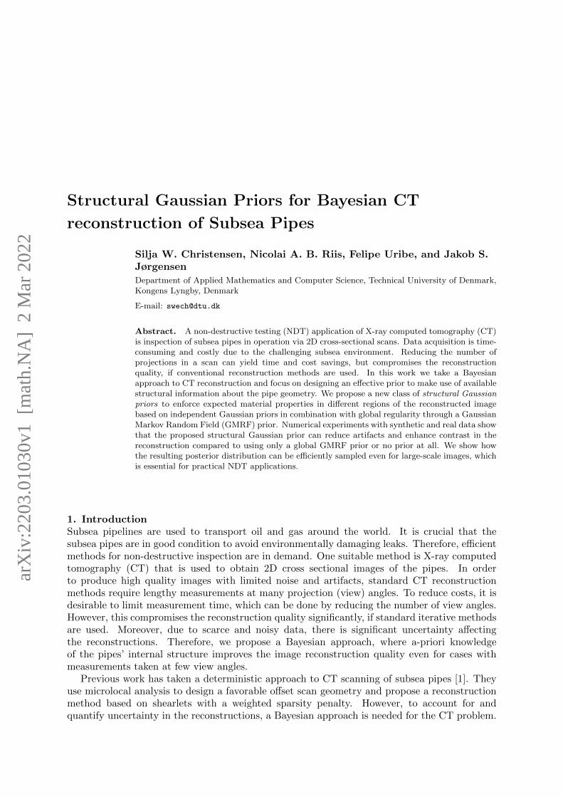
2. Bayesian CT problemDeep sea oil pipes are large and consist of dense materials including steel and concrete. Inorder to penetrate the pipe with X-rays, it is necessary to use high power and a narrow beamsource. The narrow beam can not illuminate the full pipe, but an exterior tomography setupcan be used, where the X-ray source is offset from the pipe centre, which is also the rotationaxis. Microlocal analysis shows that this setup is ideal, if we are interested in recovering thepipe and defects therein rather than the center of the pipe [1]. We use real data acquired froma prototype set-up of an oil pipe CT scanner. A detector panel with 510 sensors of sizes 0.8 mmeach was used, and 360 equi-angular projections were recorded in a full 360 degree rotation. Thepipe, its specifications, and the offset fan-beam acquisition geometry are illustrated in Figure 1.

2.1. CT modelIf we discretize the reconstruction domain in pixels, the inverse problem associated with CT canbe expressed as a linear system of equations,

d = Ax + e, e ∼ N(

0,1

λIn

), (1)

where d ∈ Rm is the observed X-ray absorption (known as a sinogram), x ∈ Rn is the unknownvector of linear attenuation coefficients in the reconstruction domain with N×N = n pixels, and

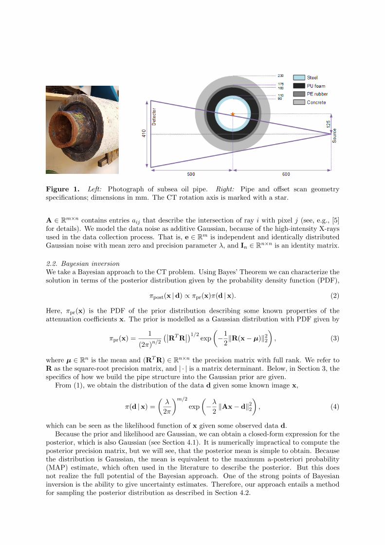
Figure 1. Left: Photograph of subsea oil pipe. Right: Pipe and offset scan geometryspecifications; dimensions in mm. The CT rotation axis is marked with a star.

A ∈ Rm×n contains entries aij that describe the intersection of ray i with pixel j (see, e.g., [5]for details). We model the data noise as additive Gaussian, because of the high-intensity X-raysused in the data collection process. That is, e ∈ Rm is independent and identically distributedGaussian noise with mean zero and precision parameter λ, and In ∈ Rn×n is an identity matrix.

2.2. Bayesian inversionWe take a Bayesian approach to the CT problem. Using Bayes’ Theorem we can characterize thesolution in terms of the posterior distribution given by the probability density function (PDF),

πpost(x |d) ∝ πpr(x)π(d |x). (2)

Here, πpr(x) is the PDF of the prior distribution describing some known properties of theattenuation coefficients x. The prior is modelled as a Gaussian distribution with PDF given by

πpr(x) =1

(2π)n/2(∣∣RTR

∣∣)1/2 exp

(−1

2‖R(x− µ)‖22

), (3)

where µ ∈ Rn is the mean and (RTR) ∈ Rn×n the precision matrix with full rank. We refer toR as the square-root precision matrix, and | · | is a matrix determinant. Below, in Section 3, thespecifics of how we build the pipe structure into the Gaussian prior are given.

From (1), we obtain the distribution of the data d given some known image x,

π(d |x) =

(λ

2π

)m/2

exp

(−λ

2‖Ax− d‖22

), (4)

which can be seen as the likelihood function of x given some observed data d.Because the prior and likelihood are Gaussian, we can obtain a closed-form expression for the

posterior, which is also Gaussian (see Section 4.1). It is numerically impractical to compute theposterior precision matrix, but we will see, that the posterior mean is simple to obtain. Becausethe distribution is Gaussian, the mean is equivalent to the maximum a-posteriori probability(MAP) estimate, which often used in the literature to describe the posterior. But this doesnot realize the full potential of the Bayesian approach. One of the strong points of Bayesianinversion is the ability to give uncertainty estimates. Therefore, our approach entails a methodfor sampling the posterior distribution as described in Section 4.2.

Figure 2. Left: Real pipe with four layers of different materials and a background of air. Right:SGP masks for i = 1, . . . , 5 that each represents a material with attenuation coefficient αi givenin (5). The white regions do not have any prior promoting specific attenuation coefficients. Theindex i = 0 is used to denote the prior on the whole image domain (background and pipe).

3. Structural Gaussian priorsWe must specify a prior in order to perform Bayesian CT reconstruction. We work with Gaussianpriors because they have nice mathematical properties making them easy to combine, andbecause they can be sampled efficiently. First, we outline the a-priori structural informationthat we have. Then we describe our proposed method of incorporating the known pipe geometryinto what we call structural Gaussian priors (SGPs). The SGP combines (stacks) priors for eachof the materials in the pipe enforcing a different prior in each region. In addition to the pipematerial and geometry information, the SGP also contains a prior on the pixel differences ofthe whole image. The purpose of this is to add a global smoothness assumption on the image,which also ensures full rank of the precision matrix of the combined Gaussian prior in (3).

3.1. A-priori structural informationWe have a-priori information about the pipe’s layered structure and constitutive materials, whichwe will incorporate in the prior model. This is the core idea of our proposed SGP. To build theSGP we need: 1) Masks for each pipe layer and for the background, and 2) estimates of thelinear attenuation coefficients of the layer materials.

3.1.1. Pipe layer masks Given p non-overlapping regions of different materials, we representeach region by a mask, i.e., a binary vector mi for i = 1, . . . , p, the same size as the imagex in which the value of element j is 1 if pixel j is in region i and 0 if not. Figure 2 showsa reconstruction of the real pipe and the corresponding masks (with p = 5). We use masksthat are slightly smaller than the actual pipe layers to account for modelling error in the pipestructure and scan geometry. The masks are constructed based on a high-quality standard CTreconstruction of the real pipe, this may also be obtained from lower-quality data or e.g. fromCAD drawings. We further define mask matrices Mi ∈ Rli×n, i = 1, . . . , p, that pick out the lipixels of region i of the n-dimensional image. Specifically, Mi is formed by keeping only the lirows of In indexed by 1-values in the mask mi.

3.1.2. Linear attenuation coefficients of pipe materials When the X-ray energy is known, wecan estimate the linear attenuation coefficients αi (ignoring scattering) for the materials as [16]:

αi = κi(E)ρi, i = 1, . . . , p, (5)

where ρi is the material density and κi(E) is the mass attenuation coefficient at X-ray energyE that can be found, e.g., in the NIST database [17].

3.2. Structural Gaussian priorsTo form the SGP we use Gaussian distributions defined in terms of means µi ∈ Rli anda symmetric positive semi-definite precision matrices

(RT

i Ri

)∈ Rn×n. In (3) we gave an

expression for Gaussians with precision matrices of full rank. When forming the SGP we willneed intrinsic Gaussians, that are also defined for rank deficient precision matrices of rankn− k > 0. The intrinsic Gaussian prior density is given [18, Ch. 3]:

πi(x) =1

(2π)(n−k)/2

(∣∣RTi Ri

∣∣∗)1/2 exp

(−1

2‖Ri(x− µi)‖22

), (6)

where | · |∗ is a generalized determinant given by the product of the n− k non-zero eigenvaluesof the precision matrix. Note this density is multivariate Gaussian if and only if k = 0. In theSGP, we use two different Gaussian priors that are specified below:

IID: The independent and identically distributed (IID) Gaussian prior is a noise dampeningprior that favors posterior pixel values around the prior mean. We use it to express a-prioriinformation of expected linear attenuation coefficients αi in the p different materials. Theprior is defined as an intrinsic Gaussian parameterized by mean and square-root precision:

µi = αi1 and Ri =√δiMi, (7)

where 1 ∈ Rli is a vector of ones and δi is a prior precision parameter.

GMRF: The Gaussian Markov Random Field (GMRF) prior is a smoothing prior thatpromotes neighbouring pixels to take the same value. The pipe materials can be consideredroughly homogeneous and therefore the GMRF prior is enforced on the entire image domain.We index this prior with i = 0 corresponding to the whole image and in this case the meanand square-root precision are:

µ0 = 0, and R0 =√δ0

[D1

D2

], (8)

where 0 ∈ Rn is a vector of zeros, D1 = IN⊗D, D2 = D⊗IN , and D ∈ R(N+1)×N is a finitedifference matrix with backward differences and zero Dirichlet boundary conditions, and ⊗denotes the Kronecker product. Note that R0 has full column rank. Then, the precisionmatrix has full rank, and the density is thus multivariate Gaussian.

To build the SGP prior, we enforce IID priors on the masked image regions and a GMRF prioron the whole image domain as described above. Under the assumption that the priors πi(x),i = 0, . . . , p are independent of each other, the SGP prior is a product of the individual priors:

πpr(x) =

p∏i=0

πi(x). (9)

Then, the prior mean and square-root precision are given:

Rpr =

R0...

Rp

and µpr =(RT

prRpr

)−1 p∑i=0

RTi Riµi. (10)

Note, that the full column rank of R0 leads to Rpr also having full column rank, and therefore

the prior precision matrix RTprRpr has full rank and is invertible.

3.2.1. SGP configurations We use the pipe shown in Figure 2 as a case study for numericalexperiments in Section 5. The pipe consists of four different materials, steel in region 2, PUfoam in region 3, PE rubber in region 4, and concrete in region 5. The pipe is scanned withair as the background and this will be denoted region 1. Thus we have p = 5 masked regionswhere we can impose IID priors promoting the expected attenuation coefficients. We study twoconfigurations of the SGP:

SGP-BG: Assuming we have information about the pipe’s dimensions but not internalstructure, we use a GMRF on the whole domain and add an IID prior on the air background(“BG”) such that πpr(x) =

∏1i=0 πi(x).

SGP-F: Assuming we also have information about the internal pipe structure, we again use aGMRF on the full (“F”) domain and add IID priors on the background and on the pipelayers such that πpr(x) =

∏5i=0 πi(x).

4. Gaussian posterior and efficient samplingIn Sections 2 and 3 we assumed Gaussian distributions for the likelihood and priors respectively,which in turn yields a Gaussian posterior PDF [2]. This is mathematically convenient becausewe can derive a closed-form expression for this distribution and sample it efficiently. Below wegive the posterior PDF and then show how to sample it by solving a system of linear equations.

4.1. Posterior PDFThe posterior PDF is given by:

πpost(x |d) ∝(λ

2π

)m2

exp

[−λ

2‖Ax− d‖22

]×

p∏i=0

(∣∣∣∣RTi Ri

2π

∣∣∣∣∗) 1

2

exp

[−1

2‖Ri(x− µi)‖22

]

∝ exp

[−λ

2‖Ax− d‖22 −

1

2

p∑i=0

‖Ri(x− µi)‖22

]. (11)

The above expression defines the Gaussian random vector

x |d ∼ N (µpost, (RTpostRpost)

−1), (12)

where the posterior square-root precision is given by

Rpost =

√λA

R0...

Rp

∈ R(m+2N(N+1)+∑p

i=1 li)×n, (13)

and the posterior mean is given implicitly by the expression:

RTpostRpostµpost = λATd +

p∑i=0

RTi Riµi. (14)

Since R0 and Rpost have full column rank, the posterior precision is invertible, and the posteriordistribution is Gaussian with well-defined covariance. That is, the closed-form expression forthe posterior distribution is (12), which can be seen by factoring out (11) and reordering theequation into the form (3).

The large-scale nature of CT makes it infeasible to form the matrix A explicitly, which isavoided by matrix-free implementations of the application of A and its adjoint. Then, theposterior mean can be obtained by solving (14). However, to compute the posterior precisionwe must form ATA, making it numerically impractical. Instead we sample the posterior asdescribed below, and statistics of the samples are used to obtain an uncertainty estimate.

4.2. Posterior SamplingOur goal is to efficiently sample the posterior (12) without explicitly forming the matrix A.Inspired by [4], we generate posterior realizations by solving the linear system of equations:

Rpostx∗ =

√λd

R0µ0...

Rpµp

+ ξ, ξ ∼ N (0, Im+2N(N+1)+∑p

i=1 li). (15)

Note that the solution method must support matrix-free implementation of A.We can show that x∗ is distributed according to the posterior by first forming the normal

equations for the linear system above, i.e.(λATA +

p∑i=0

RTi Ri

)x∗ = λATd +

p∑i=0

RTi Riµi + RT

postξ. (16)

Inserting (13) and solving for x∗ we find

x∗ =(RT

postRpost

)−1(λATd +

p∑i=0

RTi Riµi

)+(RT

postRpost

)−1RT

postξ

= µpost + R†postξ. (17)

where R†post = (RTpostRpost)

−1RTpost is the Moore–Penrose pseudoinverse. Note that x∗ is a

linear transformation of the Gaussian random variable ξ. As R0 has full column rank R†post hasfull row rank. It follows [19] that x∗ is Gaussian distributed with mean and covariance:

E(x∗) = µpost + R†post0 = µpost (18a)

Cov(x∗) = R†postI(R†post)T =

(RT

postRpost

)−1. (18b)

This confirms that x∗ is distributed according to the posterior distribution (12). That is, bysolving (15) we obtain samples of CT reconstruction images distributed according to (12).

5. Numerical ExperimentsFORCE Technology1 has provided CT data from a deep sea oil pipe acquired in a laboratoryexperiment using the offset fan-beam scan geometry illustrated in Figure 1. We conduct syntheticand real data CT experiments to assess the performance of the proposed SGPs for obtaininguseful CT reconstructions and relevant uncertainty estimates. The results are compared to aconventional deterministic reconstruction method where (1) is solved with the CGLS algorithmand stopped at semi-convergence. We interpret the posterior mean as the CT reconstructionand the posterior 95% credible interval as an associated uncertainty estimate.

5.1. Data description5.1.1. Phantom Based on the known pipe structure and materials given in Figure 2, weconstruct a phantom and corresponding SGP mask to perform synthetic experiments (see Figure3). To avoid inverse crime, the phantom is defined on a 1024 × 1024 pixel image and thereconstruction is performed on a 512 × 512 pixel image that represents a 55 × 55 cm domain

1 https://forcetechnology.com/

i Material κ[cm2/g] ρ[g/cm3] α[cm−1]

1 Air 0.044 0.0012 ∼ 02 Steel 0.042 7.9 0.163 PU foam 0.051* 0.15 0.00774 PE rubber 0.051 0.94 0.0485 Concrete 0.046 2.3 0.11

Table 1. Best estimates andprobable ranges for the materialconstants at beam intensity 2 MeV.*Estimated by PE rubber’s κ due tomissing value in database.

Figure 3. Left: Pipe phantom. Right: SGP masks for i = 1, . . . , 5 that each represents amaterial with attenuation coefficient αi given in Table 1. The white regions do not have anyprior promoting specific attenuation coefficients. The index i = 0 is used to denote the prior onthe whole image domain (background and pipe).

leading to pixels of size ∼ 1 × 1 mm. The linear attenuation coefficients in each pipe layer arecomputed according to (5) and with material constants from the NIST database [17], assuming amonochromatic beam of (mean) energy 2 MeV. The beam intensity is an estimate (in fact it is aspectrum), but around these energies the mass attenuation coefficients do not vary significantly.Therefore, we expect the computed linear attenuation coefficients are good estimates and theyare listed in Table 1. Note also that we add steel inclusions in the phantom’s concrete layer tosimulate steel reinforcement bars in the real pipe. The inclusions are in the radial or tangentialdirections and their widths are varied from 2-7 mm. With the offset scan geometry, no X-rayswill be parallel to near-radial edges, and therefore we expect that the radial inclusions are moredifficult to reconstruct than the tangential (see e.g. the discussion in [1] for more details).

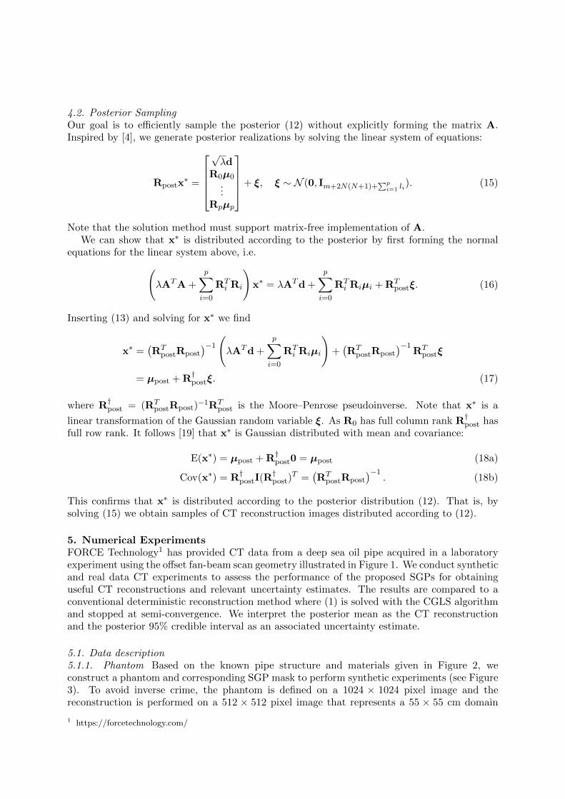
5.1.2. Sinograms Using the pipe phantom, offset acquisition geometry, and 2% noise level (i.e.‖e‖2/‖Ax‖2 ∼ 2%), we simulate a 360 view angle sinogram. Assuming the real sinogram has anequivalent noise distribution, we compare the synthetic and real data (Figure 4). Five bands inthe sinograms mark the centre region, steel, PE, PU, and concrete layers in that order from thebottom of the sinograms. The bands in the real data sinogram follow sinosoidal curves becausethe pipe center did not coincide with the rotation center, and the phases of the sinosoidal bandsvary because the pipe layers are not completely concentric. The overall similarity between thereal data and synthetic data sinograms indicates that our phantom is realistic and the scangeometry close to the real setup. For sparse view angle experiments we simulate data with only50%, 20% or 10% of the total view angles in the sinograms. Note, that because we reconstructon a 512× 512 pixel image, the CT problem is under-determined in all our experiments.

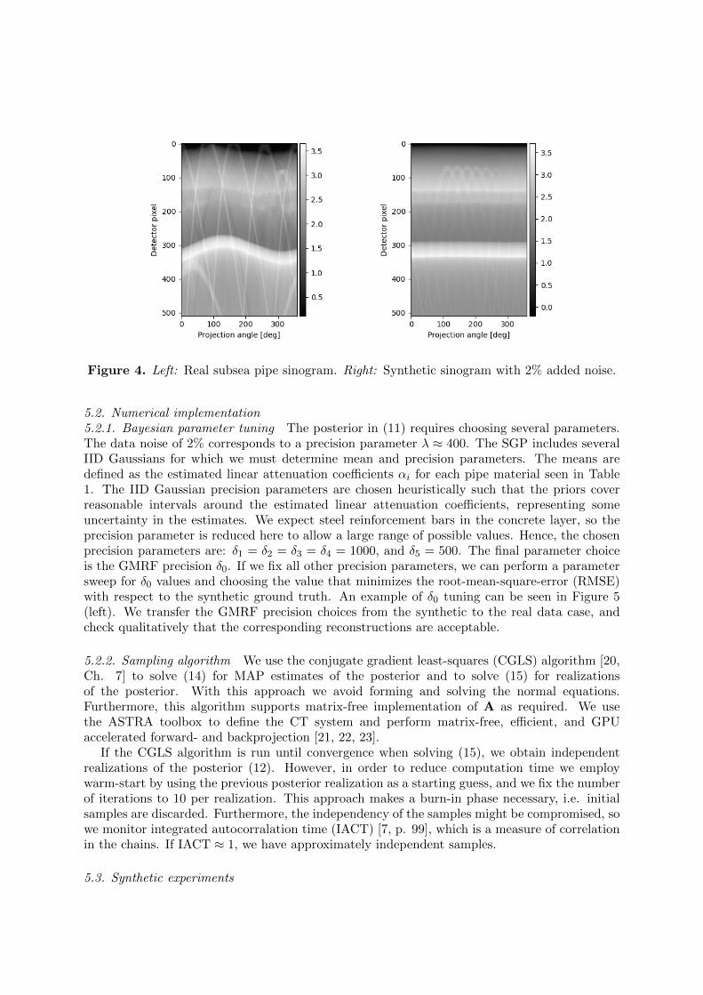
Figure 4. Left: Real subsea pipe sinogram. Right: Synthetic sinogram with 2% added noise.

5.2. Numerical implementation5.2.1. Bayesian parameter tuning The posterior in (11) requires choosing several parameters.The data noise of 2% corresponds to a precision parameter λ ≈ 400. The SGP includes severalIID Gaussians for which we must determine mean and precision parameters. The means aredefined as the estimated linear attenuation coefficients αi for each pipe material seen in Table1. The IID Gaussian precision parameters are chosen heuristically such that the priors coverreasonable intervals around the estimated linear attenuation coefficients, representing someuncertainty in the estimates. We expect steel reinforcement bars in the concrete layer, so theprecision parameter is reduced here to allow a large range of possible values. Hence, the chosenprecision parameters are: δ1 = δ2 = δ3 = δ4 = 1000, and δ5 = 500. The final parameter choiceis the GMRF precision δ0. If we fix all other precision parameters, we can perform a parametersweep for δ0 values and choosing the value that minimizes the root-mean-square-error (RMSE)with respect to the synthetic ground truth. An example of δ0 tuning can be seen in Figure 5(left). We transfer the GMRF precision choices from the synthetic to the real data case, andcheck qualitatively that the corresponding reconstructions are acceptable.

5.2.2. Sampling algorithm We use the conjugate gradient least-squares (CGLS) algorithm [20,Ch. 7] to solve (14) for MAP estimates of the posterior and to solve (15) for realizationsof the posterior. With this approach we avoid forming and solving the normal equations.Furthermore, this algorithm supports matrix-free implementation of A as required. We usethe ASTRA toolbox to define the CT system and perform matrix-free, efficient, and GPUaccelerated forward- and backprojection [21, 22, 23].

If the CGLS algorithm is run until convergence when solving (15), we obtain independentrealizations of the posterior (12). However, in order to reduce computation time we employwarm-start by using the previous posterior realization as a starting guess, and we fix the numberof iterations to 10 per realization. This approach makes a burn-in phase necessary, i.e. initialsamples are discarded. Furthermore, the independency of the samples might be compromised, sowe monitor integrated autocorralation time (IACT) [7, p. 99], which is a measure of correlationin the chains. If IACT ≈ 1, we have approximately independent samples.

5.3. Synthetic experiments

Figure 5. Left: Example of GMRF precision parameter sweep from the synthetic experiment.From this, we choose δ0 = 1000 near the minimum. Right: Examples of integratedautocorrelation time (IACT) for 100 randomly selected pixel chains.

Figure 6. Synthetic test case with 20% view angles and SGP-F prior. Left, center: 2D imagesof the posterior mean and 95% interquantile range. Right: 1D slices of posterior mean (blueline) and 95% credibility interval (blue shade), compared to ground truth (orange).

5.3.1. Example of Bayesian inversion with SGP prior We consider a sparse-angle case of only72 (20%) equi-angular projections out of the original 360. We apply the SGP-F prior to theBayesian inverse problem. First we tune the GMRF precision parameter as described above inSection 5.2.1. Figure 5 (left) illustrates the parameter sweep, and we choose δ0 = 1000, wherethe RMSE is near a minimum. Then, we compute 3000 samples from the posterior as describedin Section 5.2.2 and discard the first 1000 as burn-in. We compute IACT for 100 randomlyselected pixel chains and consider this representative. Figure 5 (right) shows that IACT is closeto or below one in all cases, indicating that the samples are approximately independent.

Figure 6 shows the posterior mean, 95% interquantile range, and 1D slices through the meanwith 95% credibility interval. We see that the pipe layers are reconstructed well. However, thesteel inclusions in the concrete layer are dampened due to the prior, that promotes concrete’sexpected linear attenuation coefficient, which is lower than that of steel. We also note highernoise in the concrete layer than the remaining parts of the reconstruction due to δ5 < δ1,...,4.The 95% interquantile range is a direct reflection of the SGP prior. We see that imposing IIDpriors in the pipe layers lowers the uncertainty estimate of the posterior compared to areaswithout IID priors imposed. Furthermore, stronger priors with high precision lead to lower

Deterministic GMRF SGP-BG SGP-F

360

vie

wan

gle

s

(RMSE = 19.5×10−3) (RMSE = 14.8×10−3) (RMSE = 9.22×10−3) (RMSE = 9.14×10−3)

50%

vie

wan

gle

s

(RMSE = 20.6×10−3) (RMSE = 16.7×10−3) (RMSE = 10.1×10−3) (RMSE = 9.91×10−3)

20%

vie

wan

gle

s

(RMSE = 25.1×10−3) (RMSE = 16.5×10−3) (RMSE = 12.2×10−3) (RMSE = 11.6×10−3)

10%

vie

wan

gle

s

(RMSE = 30.6×10−3) (RMSE = 18.9×10−3) (RMSE = 15.0×10−3) (RMSE = 12.5×10−3)

Figure 7. Posterior means and root-mean-square-error (RMSE) with increasingly informativeSGPs (in columns) and decreasing number of view angles (in rows).

uncertainty. Finally, we see that the radial steel inclusions in the concrete layer are moredifficult to reconstruct than the tangential inclusions as expected. For instance the 3 mm radialinclusion is barely distinguishable, while the 3 mm tangential inclusion is fairly clear.

5.3.2. Comparative study We investigate the effect of the SGP when reducing the number ofview angles. Figure 7 shows posterior means in a grid, where the number of view angles isdecreased across rows, and the prior information is increased across columns. We see, that as weadd structural information, the reconstructions improve in terms of 1) reduced streak artifacts,2) increased layer contrast, 3) reduced RMSE, and 4) steel inclusions that are hidden in artifactsappear when using structural information. The effect is especially clear for 10% and 20% viewangles, indicating that the structural priors are more effective in sparse view angle cases.

GMRF SGP-BG SGP-F360

vie

wan

gle

s

(δ0 = 4000) (δ0 = 4000) (δ0 = 4000)

50%

vie

wan

gle

s

(δ0 = 3000) (δ0 = 3000) (δ0 = 3000)

20%

vie

wan

gle

s

(δ0 = 10000) (δ0 = 3000) (δ0 = 1000)

10%

vie

wan

gle

s

(δ0 = 10000) (δ0 = 3000) (δ0 = 1000)

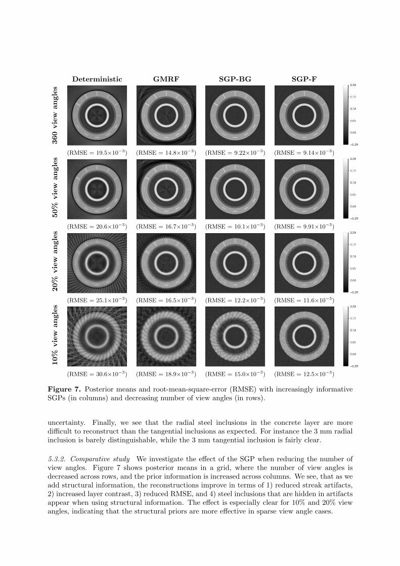
Figure 8. Posterior 95% interquantile range with increasingly informative SGPs (in columns)and decreasing number of view angles (in rows).

The deterministic reconstruction with 360 view angles produces an image where all the mainfeatures of the pipe are visible. However, we also see artifacts: 1) Along the radial steel inclusions,because these edges have no tangential rays, 2) in the centre of the image, because there is nodata, and 3) a dark ring just outside of the pipe, which is a typical artifact that appears at thefan-beam edge. As we decrease the the number of view angles, we get more dominating artifactsfrom the fan-beam edges. When we add the GMRF prior, the artifacts are smoothed out, butstill quite dominating in the image. Thus, this standard type prior is not sufficient to producegood reconstructions, especially for sparse view angles. Using the SGP-BG prior we reduce theartifacts in the background significantly. Furthermore, we see increased contrast between pipematerials. This effect is especially apparent for the 10% and 20% view angle cases. When we usethe SGP-F prior we can suppress artifacts in the background and pipe layers. In the concrete

layer, however, we see the cost. Unexpected inclusions (here steel reinforcement), that are notaccounted for in the prior, are also suppressed. Recall, that we did not impose any IID prior inboundary areas, and therefore the artifacts are not suppressed here, which we see as a “ragged”boundary, especially for sparse view angles.

We see that with the SGP-F prior we can resolve tangential steel inclusions down to widthsof 2 mm using only 20% of the view angles. The radial inclusions are well reconstructed downto 4 mm. The 2-3 mm radial inclusions are visible, but faint and blurred. Compared to thedeterministic reconstruction with no prior or to the reconstruction with GMRF prior, this is animprovement. In those cases, the narrow radial steel inclusions disappear among the artifacts.For the 10% view angles case, it becomes difficult to reconstruct any of the steel inclusions usingany of the priors. Only the widest tangential inclusions appear faintly in the reconstructions.

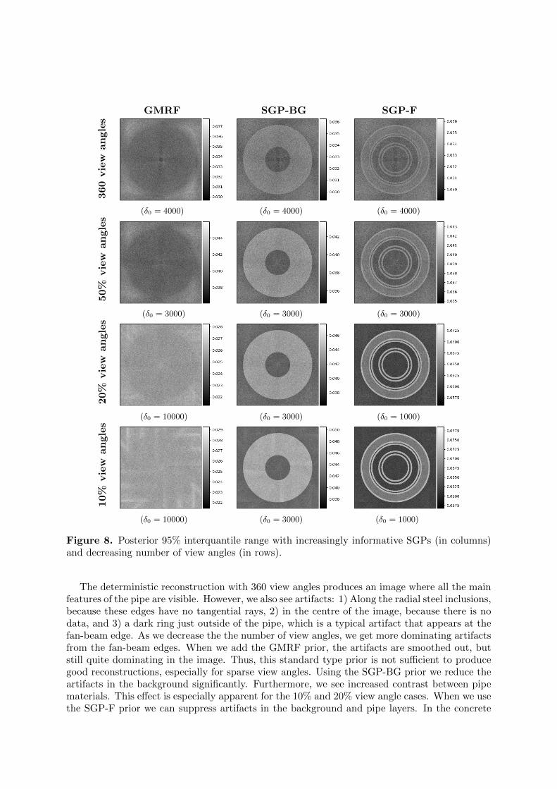
In Figure 8, we show the 95% interquantile ranges of the posteriors, which we interpretas uncertainty estimates for the reconstructions. Note that the colorbars for the images aredifferent. The GMRF prior yields an uncertainty pattern reflecting the acquisition geometry andcorresponds to the structure of the likelihood. For the SGP priors the uncertainty pattern reflectsthe structure in the prior. For SGP-F, we observe lowest uncertainty in the background and inthe steel, PU, and PE layers (regions 1-4), where we find the highest prior precision parameters.The concrete layer (region 5) has a lower prior precision, and thus a higher uncertainty. Thehighest uncertainty is found in the boundary regions, where no particular attenuation coefficientis promoted. We note that the boundary regions seem to have relatively higher uncertainty for10% and 20% view angles, than for 50% and 100%. This is caused by the lower GMRF precisionδ0 for the two former cases. Finally, the likelihood structure is visible for the SGP-F prior caseswith 50% and 100% view angles, but not with 10% and 20%. We suspect that this is due to theprior having a relatively larger influence than the likelihood, when there is sparse data.

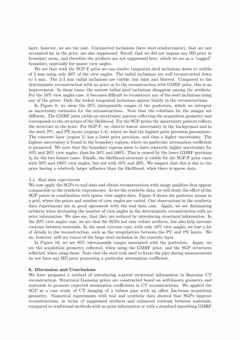
5.4. Real data experimentsWe now apply the SGPs to real data and obtain reconstructions with image qualities that appearcomparable to the synthetic experiments. As for the synthetic data, we will study the effect of theSGP priors in combination with sparse view angles data. Figure 9 shows the posterior means ina grid, where the priors and number of view angles are varied. Our observations in the syntheticdata experiments are in good agreement with the real data case. Again, we see dominatingartifacts when decreasing the number of view angles in the deterministic reconstruction with noprior information. We also see, that they are reduced by introducing structural information. Inthe 20% view angles case, we see that the SGPs not only reduce artifacts, but also help increasecontrast between materials. In the most extreme case, with only 10% view angles, we lose a lotof details in the reconstruction, such as the irregularities between the PU and PE layers. Wedo, however, still see traces of the large steel inclusion in the concrete layer.

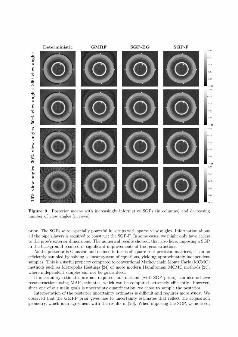
In Figure 10, we see 95% interquantile ranges associated with the posteriors. Again, wesee the acquisition geometry reflected, when using the GMRF prior, and the SGP structuresreflected, when using those. Note that the steel rods used to fixate the pipe during measurementsdo not have any IID prior promoting a particular attenuation coefficient.

6. Discussion and ConclusionsWe have proposed a method of introducing a-priori structural information in Bayesian CTreconstruction. Structural Gaussian priors are constructed based on well-known geometry andmaterials to promote expected attenuation coefficients in CT reconstructions. We applied theSGP in a case study of CT imaging of a subsea pipe with an offset fan-beam acquisitiongeometry. Numerical experiments with real and synthetic data showed that SGPs improvereconstructions, in terms of suppressed artifacts and enhanced contrast between materials,compared to traditional methods with no prior information or with a standard smoothing GMRF

Deterministic GMRF SGP-BG SGP-F

360

vie

wan

gle

s50%

vie

wan

gle

s20%

vie

wan

gle

s10%

vie

wan

gle

s

Figure 9. Posterior means with increasingly informative SGPs (in columns) and decreasingnumber of view angles (in rows).

prior. The SGPs were especially powerful in setups with sparse view angles. Information aboutall the pipe’s layers is required to construct the SGP-F. In some cases, we might only have accessto the pipe’s exterior dimensions. The numerical results showed, that also here, imposing a SGPin the background resulted in significant improvements of the reconstructions.

As the posterior is Gaussian and defined in terms of square-root precision matrices, it can beefficiently sampled by solving a linear system of equations, yielding approximately independentsamples. This is a useful property compared to conventional Markov chain Monte Carlo (MCMC)methods such as Metropolis Hastings [24] or more modern Hamiltonian MCMC methods [25],where independent samples can not be guaranteed.

If uncertainty estimates are not required, our method (with SGP priors) can also achievereconstructions using MAP estimates, which can be computed extremely efficiently. However,since one of our main goals is uncertainty quantification, we chose to sample the posterior.

Interpretation of the posterior uncertainty estimates is difficult and requires more study. Weobserved that the GMRF prior gives rise to uncertainty estimates that reflect the acquisitiongeometry, which is in agreement with the results in [26]. When imposing the SGP, we noticed,

GMRF SGP-BG SGP-F360

vie

wan

gle

s

(δ0 = 4000) (δ0 = 4000) (δ0 = 4000)

50%

vie

wan

gle

s

(δ0 = 3000) (δ0 = 3000) (δ0 = 3000)

20%

vie

wan

gle

s

(δ0 = 10000) (δ0 = 3000) (δ0 = 1000)

10%

vie

wan

gle

s

(δ0 = 10000) (δ0 = 3000) (δ0 = 1000)

Figure 10. Real data: Posterior 95% interquantile range with increasingly informative SGPs(in columns) and decreasing number of view angles (in rows).

that the uncertainty estimates directly reflected the prior. The prior’s effect on the uncertaintyestimates have also been seen in other studies. For instance, edge-preserving priors give rise tohigh uncertainty on discontinuities in CT reconstructions [3, 4]. In future work we aim to furtherimprove uncertainty estimates of the pipe and defect structure, for example to help distinguishartifacts from real features in the reconstruction.

AcknowledgmentsThis work was supported by The Villum Foundation (grant no. 25893). We also thank FORCETechnology for providing real data and information regarding subsea pipes.

References[1] Riis N A B, Frøsig J, Dong Y and Hansen P C 2018 Limited-data x-ray CT for underwater pipeline inspection

Inverse Problems 34 034002[2] Kaipio J and Somersalo E 2005 Statistical and Computational Inverse Problems (Dordrecht: Springer)[3] Suuronen J, Emzir M, Lasanen S, Sarkka S and Roininen L 2020 Enhancing industrial x-ray tomography by

data-centric statistical methods Data-Centric Engineering 1 e10[4] Uribe F, Bardsley J, Dong Y, Hansen P C and Riis N 2021 A hybrid gibbs sampler for edge-preserving

tomographic reconstruction with uncertain view angles (Preprint arXiv:2104.06919)[5] Hansen P C, Jørgensen J S and Lionheart W R B (eds) 2021 Computed Tomography: Algorithms, Insight,

and Just Enough Theory (Philadelphia: SIAM)[6] Sidky E Y and Pan X 2008 Image reconstruction in circular cone-beam computed tomography by constrained,

total-variation minimization Physics in Medicine & Biology 53 4777[7] Bardsley J M 2018 Uncertainty Quantification for Inverse Problems (Philadelphia: SIAM)[8] Bardsley J M 2013 Gaussian Markov random field priors for inverse problems Inverse Problems and Imaging

7 397–416[9] Bardsley J M 2012 Laplace-distributed increments, the laplace prior, and edge-preserving regularization

Journal of Inverse and Ill-Posed Problems 20 271–285[10] Markkanen M, Roininen L, Huttunen J M J and Lasanen S 2019 Cauchy difference priors for edge-preserving

Bayesian inversion Journal of Inverse and Ill-posed Problems 27 225–240[11] Zhang H, Han H, Ma J, Liu Y, Moore W and Liang Z 2014 Deriving adaptive MRF coefficients from previous

normal-dose CT scan for low-dose image reconstruction via penalized weighted least-squares minimizationMedical physics 41 041916

[12] Zhang H, Han H, Liang Z, Hu Y, Liu Y, Moore W, Ma J and Lu H 2016 Extracting information fromprevious full-dose CT scan for knowledge-based Bayesian reconstruction of current low-dose CT imagesIEEE Transactions on Medical Imaging 35 860–870

[13] Han H, Zhang H, Wei X, Moore W and Liang Z 2016 Medical Imaging 2016: Physics of Medical Imaging p97834F

[14] Gao Y, Liang Z, Moore W, Zhang H, Pomeroy M, Ferretti J, Bilfinger T, Ma J and Lu H 2019 A feasibilitystudy of extracting tissue textures from a previous full-dose CT database as prior knowledge for Bayesianreconstruction of current low-dose CT images IEEE Transactions on Medical Imaging 38 1981–1992

[15] Fukuda W, Maeda S i, Kanemura A and Ishii S 2010 2010 IEEE International Conference on Acoustics,Speech and Signal Processing pp 2126–2129

[16] Buzug T and Tomography C 2008 From photon statistics to modern cone-beam CT (Berlin: Springer)[17] Hubbell J H and Seltzer S M 2004 Tables of x-ray mass attenuation coefficients and mass energy-absorption

coefficients (version 1.4) [Online] Available: https://dx.doi.org/10.18434/T4D01F. Accessed: 2021-01-19.

[18] Rue H and Held L Gaussian Markov Random Fields Theory and Applications (New York: Chapman &Hall/CRC) ISBN 1-54488-432-0

[19] Bickel P and Doksum K 2001 Mathematical Statistics: Basic Ideas and Selected Topics. 2nd ed vol 1 (NewJersey: Prentice Hall)

[20] Bjorck A 1996 Numerical Methods for Least Squares Problems (Philadelphia: SIAM)[21] van Aarle W, Palenstijn W J, Cant J, Janssens E, Bleichrodt F, Dabravolski A, Beenhouwer J D, Batenburg

K J and Sijbers J 2016 Fast and flexible x-ray tomography using the ASTRA toolbox Opt. Express 2425129–25147

[22] van Aarle W, Palenstijn W J, De Beenhouwer J, Altantzis T, Bals S, Batenburg K J and Sijbers J2015 The astra toolbox: A platform for advanced algorithm development in electron tomographyUltramicroscopy 157 35–47 ISSN 0304-3991 URL https://www.sciencedirect.com/science/article/

pii/S0304399115001060

[23] Palenstijn W J, Batenburg K J and Sijbers J 2011 Performance improvements for iterative electrontomography reconstruction using graphics processing units (GPUs) Journal of Structural Biology 176250–253 ISSN 1047-8477

[24] Hastings W K 1970 Monte carlo sampling methods using Markov chains and their applications Biometrika57 97–109

[25] Duane S, Kennedy A, Pendleton B J and Roweth D 1987 Hybrid monte carlo Physics Letters B 195 216–222ISSN 0370-2693

[26] Bardsley J M 2012 MCMC-based image reconstruction with uncertainty quantification SIAM Journal onScientific Computing 34 A1316–A1332