A MULTISCALE ALGORITHM FOR IMAGE SEGMENTATION BYVARIATIONAL METHOD.G. KOEPFLER� , C. LOPEZy , AND J.M. MORELyAbstract. Most segmentation algorithms are composed of several procedures: split and merge,small region elimination, boundary smoothing, : : : , each depending on several parameters. The in-troduction of an energy to minimize leads to a drastic reduction of these parameters. We prove thatthe most simple segmentation tool, the \region merging" algorithm, made according to the simplestenergy, is enough to compute a local energy minimum belonging to a compact class and to achieve thejob of most of the tools mentioned above. We explain why \merging" in a variational framework leadsto a fast multiscale, multichannel algorithm, with a pyramidal structure. The obtained algorithm isO(n ln n), where n is the number of pixels of the picture. We apply this fast algorithm to make greylevel and texture segmentation and we show experimental results.Key words. variational methods, nonnumerical algorithm, image processing, texture discrimina-tionAMS(MOS) subject classi�cations. 68Q20,68U10,1. Introduction. The aim of this paper is to describe a fast and universal imagesegmentation algorithm. Properties of this algorithm, are :It is multiscale and pyramidal. In other terms, it will not only compute onesegmentation, but a hierarchy of segmentations from �ne to coarse scales. Moreoverthe coarser segmentation will be deduced from the �ner by \merging" operations, witha pyramidal structure for the computation. This corresponds to Marr's remark [Marr]that textures \live" at several scales. Therefore, a discrimination algorithm shouldgive di�erent kinds of segmentations which depend on the scale.As a consequence of this pyramidal structure, the computation time is in practiceproportional to the size of the datum. Moreover, this algorithmic structure will makeit accessible to e�cient hardware implementation.The algorithm is universal, that is, does not depend on any a priori knowledgeon the statistics of the image. Texture discrimination is achieved according to auniversal criterion depending on very few parameters. More precisely, a picture isde�ned by a certain number of \channels" (grey level, colour levels, integrodi�erentialchannels obtained by fast wavelet transform). In our segmentation algorithm, the onlyparameters are the weights attached to each channel, that is, the importance given toeach channel as a segmentation criterion. However these parameters can be �xed oncefor all with reliable results.The algorithm has been constructed by making a synthesis of several theories : thetextons theory of Julesz [Ju], the energy methods in image segmentation introducedby Geman and Geman [GemG], Blake and Zisserman [BlakZ], Mumford and Shah[MumS1] , the Wavelet transform theory of Meyer [Me] , Mallat [Mall] and Cohen[Coh] , which uni�es the theory of recursive �ltering and pyramidal schemes.The segmentations provided by the algorithm will be proved to have a large rangeof good topological and numerical properties, including compactness of the set ofapproximate solutions, convergence of minimizing sequences made of �ner and �ner� COGNITECH, Inc., Santa Monica (CA), now at: U.F.R. de Math�ematiques et Informatique,University Paris V-Ren�e Descartes 75270 Paris Cedex 06, Francey CEREMADE, University Paris IX-Dauphine 75775 Paris Cedex 16, France1

solutions, smoothness of the locally optimal solutions, completeness of the multiscalerepresentation, a priori estimates on the size of the regions of the segmentations.2. General principles of segmentation devices.2.1. Formalization. We de�ne an image g as a scalar function, de�ned on theimage domain (generally a rectangle). The function g may also be vectorial, in thecase where it has several channels for characterizing textures, histograms, colors, : : :That does not change anything in the theorems and proofs that we later state. Theonly hypothesis is that these channels have been de�ned in order to be good indicatorsof the similarity { or di�erence { of points of the picture, and therefore good indicatorsfor the autosimilarity of regions. We seek for a segmentation, that is, a partition ofthis rectangle into a �nite set of regions, each of which corresponds to a part of theimage where g is as constant as possible. Moreover, we wish to compute explicitly theregion boundaries and of course control their regularity and location.More precisely we will adopt the following principles.The �rst principle is that the boundary detection problem must follow some uni-versal rules. In other terms, we admit the possibility of a universal boundary detectiondevice, de�nable and analyzable independently from the kind of channels (grey level,colour, texture, : : :) to be used as input for the segmentation ([BecSI, MaliP2, Ju]).This �rst principle allows us to try to get a complete mathematical understandingof the segmentation problem, by considering the grey level segmentation. It is thesimplest case of boundary detection, and it eliminates every early discussion aboutthe concept of texture. (By \boundary in an image", we mean the boundary in thetopological sense : it is the boundary of an homogeneous region of the image. Thusboundaries are di�erent from edges obtained by some local �ltering.)A second principle which we adopt in the following is that an algorithm for bound-ary detection must be scale and space invariant. By space invariance, we mean thatall points of the analyzed picture will be treated on the same way, and therefore a seg-mentation device must be translation and rotation invariant. Since boundaries maybe present at every \scale", the scale invariance only means that we shall considermultiscale segmentation algorithms, depending on a scale parameter � which we donot try to estimate and leave to the user's choice.Finally we shall adopt a principle without which no discussion about segmentationcan even start, and which we call comparison principle. It states that given twodi�erent segmentations of a datum, we are always able to decide which of them isconsidered as better than (or equivalent to) the other. Thus we assume the existenceof some total ordering over all possible segmentations, and this can be simply achievedonly if this ordering is re ected by some real functional E such that if E(K1) < E(K2),then the segmentationK1 has to be considered \better" than the segmentationK2. Forinstance, this principle is veri�ed by segmentation devices based on some Gibbs energyfunctional like in [GemG]. It is not veri�ed by the region growing methods based onthresholds [Pav1, Pav2, PavL, Zu], nor by the edge detection devices [Marr, MaliP1].Since, by the comparison principle, all of these criteria must be taken into ac-count in the functional E, we see that this functional necessarily contains terms whichcontrol:- the autosimilarity of each region with respect to the chosen channels. Thosechannels must be as constant as possible on each region.- the size, location and regularity of the boundaries.2

Denote by K the whole boundary set of the segmentation. According to these prin-ciples, a natural energy functional for segmentation will contain two terms, a twodimensional term for the autosimilarity of the regions which will roughly speakingmeasure the variance of g on each connected component of nK and a one dimen-sional one for controlling the length, and eventually the adequacy of location of theboundaries. Such a generic justi�cation is developed e.g. in [MumS1, MumS2]. Bythe space invariance principle, those terms will be integral terms, the two dimensionalone being an integral with respect to the Lebesgue measure and the one dimensionalan integral with respect to the Hausdor� measure or \length" along the boundaries.Clearly, the weights given to the terms of the functional will be left to our choice.Consider for example the energy used by Mumford and Shah :E(u;K) = ZnK jruj2dx+ Z(u� g)2dx+ ZK d� ;Both �rst integrals are bidimensional and the third one is with respect to the uniformmeasure d� supported by K. This energy means that in a \good" segmentation (u;K),the curves of K should be the boundaries of homogeneous regions in the image andu a sort of mean or, more generally, a regularized version of g in the interior of suchareas (as illustration see the cartographical application in �gure 4.1, u is choosen tobe piecewise constant). The third term gives a control on the length, and thereforeon the regularity of the boundaries of K ( see below ). This kind of functional repre-sents of course a compromise between accuracy of the regions and parsimony of theboundaries: in case of grey level segmentation, as noticed in Zucker [Zu] or Haralickand Shapiro [HarS], a pure region growing would simply put together the pixels withsimilar grey levels. But this generates very nonsmooth boundaries and therefore also\small" or \thin" regions.So if no control is made on the boundaries, one needs additional criteria and thresh-olding to achieve a decent segmentation. A functional like the above functional isdesigned to avoid this kind of mixed methods : one hopes having all the criteria puttogether in the same functional. For instance, the functional used for the so called\snakes" [KasWT, AmiTW] uses a more sophisticated third term for controlling bothlocation (the boundary, or \snake", is forced to be close to edges) and smoothnessof the boundary. Many early functionals in image analysis had only two dimensionalenergy terms (which were coupled with some thresholding criteria [Pav1, Zu]).2.2. Choice of properties and algorithms for segmentation. The algorith-mic description given by Pavlidis and Liow [PavL] is an excellent illustration of thelevel of sophistication to which the segmentation methods have arrived in ComputerVision, by superposing several tricky devices arisen in the two last decades. Now, thequestion which is naturally raised by the coexistence of energy functionals on one side,and of segmentation devices on the other is whether they match in any aspect, andhow.Our purpose is to classify the properties which are sought by those devices andto decide which of them are basic, and which can be deduced. Beyond being a wayto attain certainty, mathematical proofs are a powerful tool for obtaining such a clas-si�cation of properties. Once this hierarchy among tools has been established, onemay hope to simplify the algorithms and to make them completely transmissible andreproducible. Our aim in this paper is to apply this method and to classify terms3

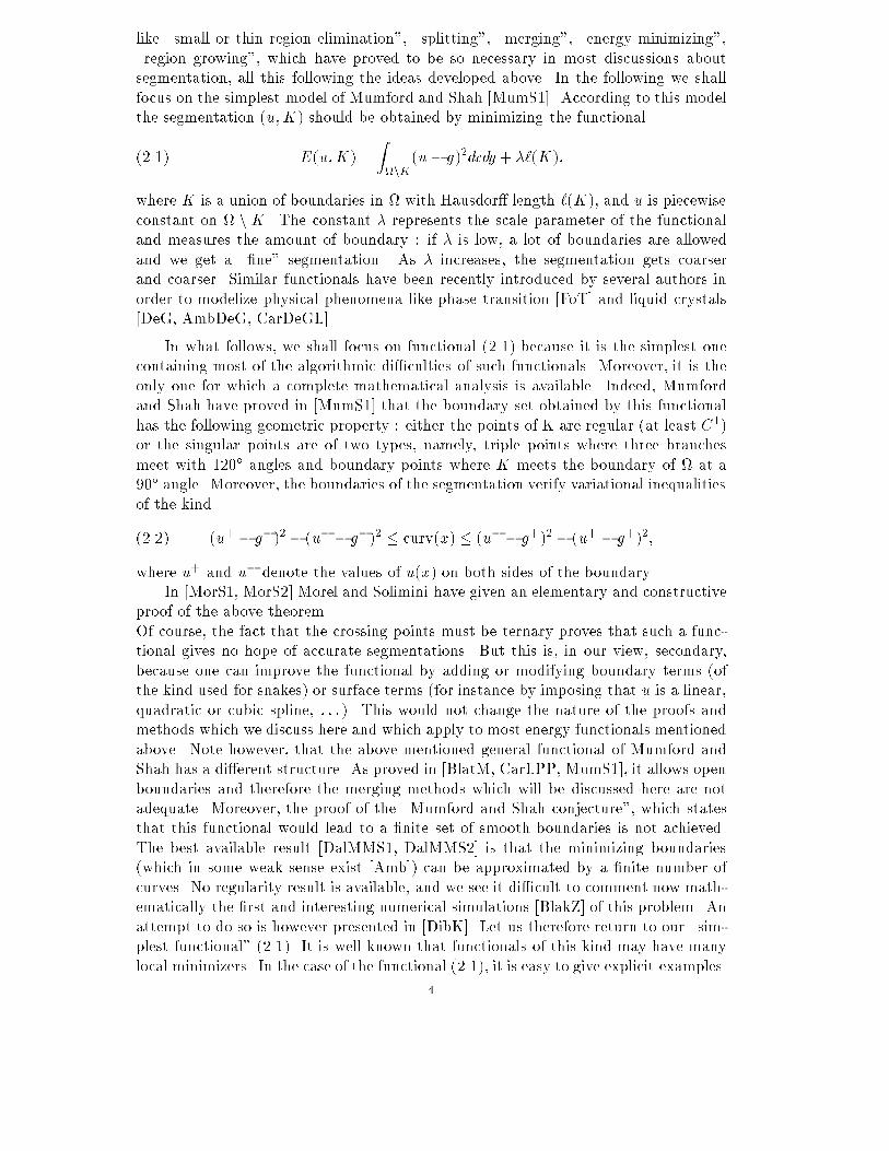
like \small or thin region elimination", \splitting", \merging", \energy minimizing",\region growing", which have proved to be so necessary in most discussions aboutsegmentation, all this following the ideas developed above. In the following we shallfocus on the simplest model of Mumford and Shah [MumS1]. According to this modelthe segmentation (u;K) should be obtained by minimizing the functionalE(u;K) = ZnK(u� g)2dxdy + �`(K);(2.1)where K is a union of boundaries in with Hausdor� length `(K), and u is piecewiseconstant on nK. The constant � represents the scale parameter of the functionaland measures the amount of boundary : if � is low, a lot of boundaries are allowedand we get a \�ne" segmentation. As � increases, the segmentation gets coarserand coarser. Similar functionals have been recently introduced by several authors inorder to modelize physical phenomena like phase transition [FoT] and liquid crystals[DeG, AmbDeG, CarDeGL] .In what follows, we shall focus on functional (2.1) because it is the simplest onecontaining most of the algorithmic di�culties of such functionals. Moreover, it is theonly one for which a complete mathematical analysis is available. Indeed, Mumfordand Shah have proved in [MumS1] that the boundary set obtained by this functionalhas the following geometric property : either the points of K are regular (at least C1)or the singular points are of two types, namely, triple points where three branchesmeet with 120� angles and boundary points where K meets the boundary of at a90� angle. Moreover, the boundaries of the segmentation verify variational inequalitiesof the kind(u+ � g�)2 � (u� � g�)2 � curv(x) � (u� � g+)2 � (u+ � g+)2;(2.2)where u+ and u� denote the values of u(x) on both sides of the boundary.In [MorS1, MorS2] Morel and Solimini have given an elementary and constructiveproof of the above theorem.Of course, the fact that the crossing points must be ternary proves that such a func-tional gives no hope of accurate segmentations. But this is, in our view, secondary,because one can improve the functional by adding or modifying boundary terms (ofthe kind used for snakes) or surface terms (for instance by imposing that u is a linear,quadratic or cubic spline, : : :). This would not change the nature of the proofs andmethods which we discuss here and which apply to most energy functionals mentionedabove. Note however, that the above mentioned general functional of Mumford andShah has a di�erent structure. As proved in [BlatM, CarLPP, MumS1], it allows openboundaries and therefore the merging methods which will be discussed here are notadequate. Moreover, the proof of the \Mumford and Shah conjecture", which statesthat this functional would lead to a �nite set of smooth boundaries is not achieved.The best available result [DalMMS1, DalMMS2] is that the minimizing boundaries(which in some weak sense exist [Amb]) can be approximated by a �nite number ofcurves. No regularity result is available, and we see it di�cult to comment now math-ematically the �rst and interesting numerical simulations [BlakZ] of this problem. Anattempt to do so is however presented in [DibK]. Let us therefore return to our \sim-plest functional" (2.1). It is well known that functionals of this kind may have manylocal minimizers. In the case of the functional (2.1), it is easy to give explicit examples.4

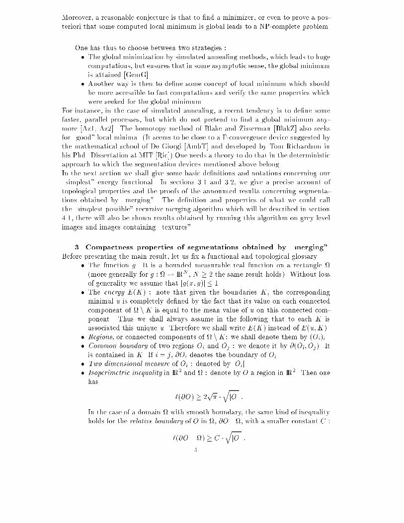
Moreover, a reasonable conjecture is that to �nd a minimizer, or even to prove a pos-teriori that some computed local minimum is global leads to a NP-complete problem.One has thus to choose between two strategies :� The global minimization by simulated annealing methods, which leads to hugecomputations, but ensures that in some asymptotic sense, the global minimumis attained [GemG].� Another way is then to de�ne some concept of local minimum which shouldbe more accessible to fast computations and verify the same properties whichwere seeked for the global minimum.For instance, in the case of simulated annealing, a recent tendency is to de�ne somefaster, parallel processes, but which do not pretend to �nd a global minimum any-more [Az1, Az2]. The homotopy method of Blake and Zisserman [BlakZ] also seeksfor \good" local minima. (It seems to be close to a �-convergence device suggested bythe mathematical school of De Giorgi [AmbT] and developed by Tom Richardson inhis Phd. Dissertation at MIT [Ric]).One needs a theory to do that in the deterministicapproach to which the segmentation devices mentioned above belong.In the next section we shall give some basic de�nitions and notations concerning our\simplest" energy functional. In sections 3.1 and 3.2, we give a precise account oftopological properties and the proofs of the announced results concerning segmenta-tions obtained by \merging". The de�nition and properties of what we could callthe \simplest possible" recursive merging algorithm which will be described in section4.1, there will also be shown results obtained by running this algorithm on grey levelimages and images containing \textures".3. Compactness properties of segmentations obtained by \merging".Before presenting the main result, let us �x a functional and topological glossary.� The function g. It is a bounded measurable real function on a rectangle (more generally for g : 7! IRN , N � 2 the same result holds). Without lossof generality we assume that jg(x; y)j � 1.� The energy E(K) : note that given the boundaries K, the correspondingminimal u is completely de�ned by the fact that its value on each connectedcomponent of nK is equal to the mean value of u on this connected com-ponent. Thus we shall always assume in the following that to each K isassociated this unique u. Therefore we shall write E(K) instead of E(u;K).� Regions, or connected components of nK: we shall denote them by (Oi)i.� Common boundary of two regions Oi and Oj : we denote it by @(Oi; Oj). Itis contained in K. If i = j, @Oi denotes the boundary of Oi.� Two dimensional measure of Oi : denoted by jOij.� Isoperimetric inequality in IR2 and : denote by O a region in IR2. Then onehas `(@O) � 2p� �qjOj :In the case of a domain with smooth boundary, the same kind of inequalityholds for the relative boundary of O in , @O\, with a smaller constant C :`(@O \ ) � C �qjOj :5

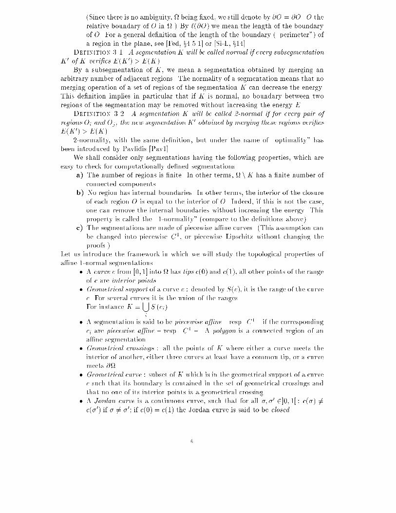
(Since there is no ambiguity, being �xed, we still denote by @O = @O\O therelative boundary of O in .) By `(@O) we mean the length of the boundaryof O. For a general de�nition of the length of the boundary (\perimeter") ofa region in the plane, see [Fed, x4.5.1] or [Si-L, x14].Definition 3.1. A segmentationK will be called normal if every subsegmentationK 0 of K veri�es E(K 0) > E(K).By a subsegmentation of K, we mean a segmentation obtained by merging anarbitrary number of adjacent regions. The normality of a segmentation means that nomerging operation of a set of regions of the segmentation K can decrease the energy.This de�nition implies in particular that if K is normal, no boundary between tworegions of the segmentation may be removed without increasing the energy E.Definition 3.2. A segmentation K will be called 2-normal if for every pair ofregions Oi and Oj, the new segmentation K 0 obtained by merging these regions veri�esE(K 0) > E(K).2-normality, with the same de�nition, but under the name of \optimality" hasbeen introduced by Pavlidis [Pav1].We shall consider only segmentations having the following properties, which areeasy to check for computationally de�ned segmentations.a) The number of regions is �nite. In other terms, nK has a �nite number ofconnected components.b) No region has internal boundaries. In other terms, the interior of the closureof each region O is equal to the interior of O. Indeed, if this is not the case,one can remove the internal boundaries without increasing the energy. Thisproperty is called the \1-normality" (compare to the de�nitions above).c) The segmentations are made of piecewise a�ne curves. (This assumption canbe changed into piecewise C1, or piecewise Lipschitz without changing theproofs.)Let us introduce the framework in which we will study the topological properties ofa�ne 1-normal segmentations.� A curve c from [0; 1] into has tips c(0) and c(1), all other points of the rangeof c are interior points.� Geometrical support of a curve c : denoted by S(c), it is the range of the curvec. For several curves it is the union of the ranges.For instance K =[i S (ci).� A segmentation is said to be piecewise a�ne { resp. C1 { if the correspondingci are piecewise a�ne { resp. C1 {. A polygon is a connected region of ana�ne segmentation.� Geometrical crossings : all the points of K where either a curve meets theinterior of another, either three curves at least have a common tip, or a curvemeets @.� Geometrical curve : subset of K which is in the geometrical support of a curvec such that its boundary is contained in the set of geometrical crossings andthat no one of its interior points is a geometrical crossing.� A Jordan curve is a continuous curve, such that for all �; �0 2]0; 1[ : c(�) 6=c(�0) if � 6= �0; if c(0) = c(1) the Jordan curve is said to be closed.6

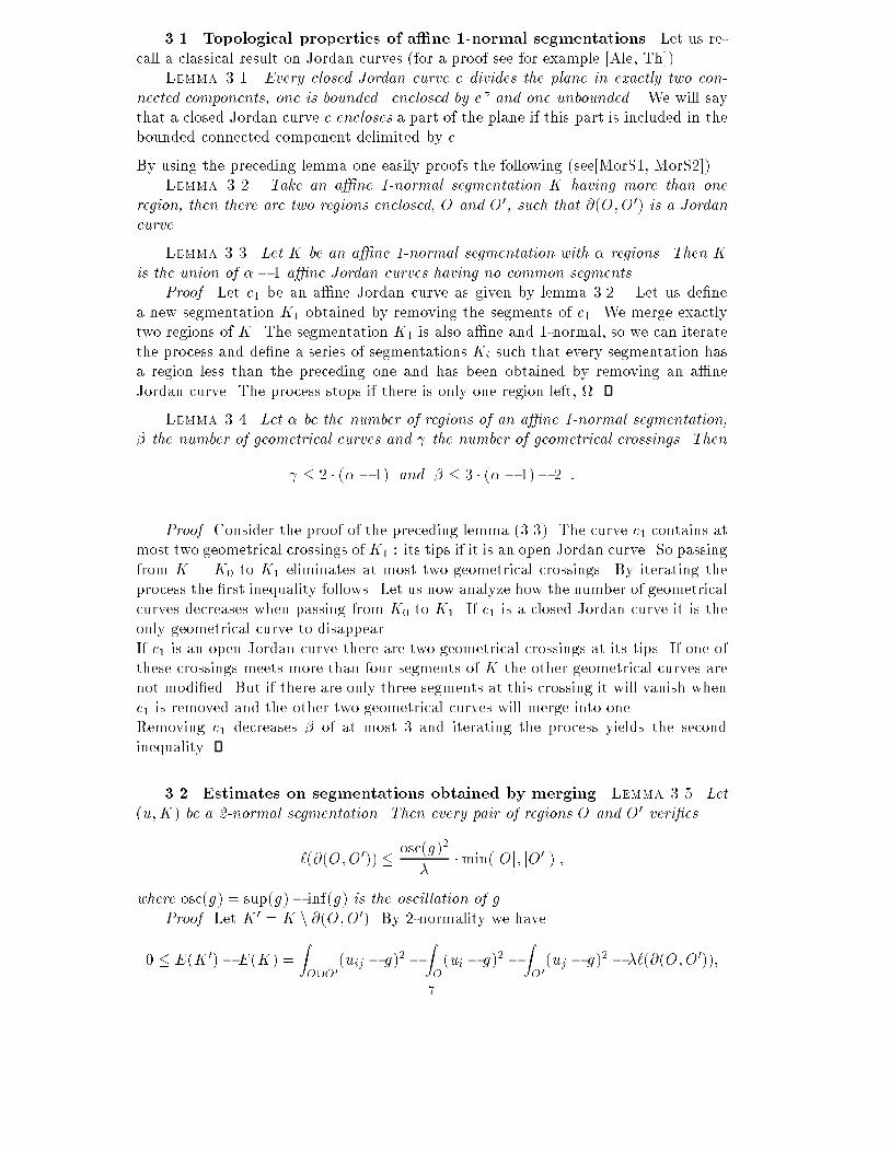
3.1. Topological properties of a�ne 1-normal segmentations. Let us re-call a classical result on Jordan curves (for a proof see for example [Ale, Th])Lemma 3.1. Every closed Jordan curve c divides the plane in exactly two con-nected components, one is bounded \enclosed by c" and one unbounded. We will saythat a closed Jordan curve c encloses a part of the plane if this part is included in thebounded connected component delimited by c.By using the preceding lemma one easily proofs the following (see[MorS1, MorS2]).Lemma 3.2. Take an a�ne 1-normal segmentation K having more than oneregion, then there are two regions enclosed, O and O0, such that @(O;O0) is a Jordancurve.Lemma 3.3. Let K be an a�ne 1-normal segmentation with � regions. Then Kis the union of �� 1 a�ne Jordan curves having no common segments.Proof. Let c1 be an a�ne Jordan curve as given by lemma 3.2 . Let us de�nea new segmentation K1 obtained by removing the segments of c1. We merge exactlytwo regions of K. The segmentation K1 is also a�ne and 1-normal, so we can iteratethe process and de�ne a series of segmentations Ki such that every segmentation hasa region less than the preceding one and has been obtained by removing an a�neJordan curve. The process stops if there is only one region left, .Lemma 3.4. Let � be the number of regions of an a�ne 1-normal segmentation,� the number of geometrical curves and the number of geometrical crossings. Then � 2 � (�� 1) and � � 3 � (�� 1)� 2 :Proof. Consider the proof of the preceding lemma (3.3). The curve c1 contains atmost two geometrical crossings ofK1 : its tips if it is an open Jordan curve. So passingfrom K = K0 to K1 eliminates at most two geometrical crossings. By iterating theprocess the �rst inequality follows. Let us now analyze how the number of geometricalcurves decreases when passing from K0 to K1. If c1 is a closed Jordan curve it is theonly geometrical curve to disappear.If c1 is an open Jordan curve there are two geometrical crossings at its tips. If one ofthese crossings meets more than four segments of K the other geometrical curves arenot modi�ed. But if there are only three segments at this crossing it will vanish whenc1 is removed and the other two geometrical curves will merge into one.Removing c1 decreases � of at most 3 and iterating the process yields the secondinequality.3.2. Estimates on segmentations obtained by merging. Lemma 3.5. Let(u;K) be a 2-normal segmentation. Then every pair of regions O and O0 veri�es`(@(O;O0)) � osc(g)2� �min(jOj; jO0j) ;where osc(g) = sup(g)� inf(g) is the oscillation of g.Proof. Let K 0 = K n @(O;O0). By 2-normality we have0 � E(K 0)� E(K) = ZO[O0(uij � g)2� ZO(ui � g)2 � ZO0(uj � g)2 � �`(@(O;O0));7

where ui, uj and uij are the mean values of g on O, O0 and O[O0. We get, supposingfor example that jOj � jO0j,� � `(@(O;O0)) � ZO h(uij � g)2 � (ui � g)2i� min(jOj; jO0j) osc(g)2Lemma 3.6. For every region O of a 2-normal segmentation, denote by N(O) thenumber of neighbouring regions. ThenN(O) � C�pjOj osc(g)2 ;where C is the isoperimetric constant in .Proof. Call Oj a neighbouring region of O. The fact that O and Oj cannot bemerged without increasing the energy E implies that� ` (@ (O;Oj)) � jOj osc(g)2:Thus by adding these inequalities for all neighbours of O, we obtain� `(@O) � N(O)jOj osc(g)2:We conclude by applying to O the isoperimetric inequality in .Lemma 3.7. Let � be the number of regions of a 2-normal a�ne segmentation.Then � � 288 jj osc(g)4C2�2 :Proof. The union of all regions Oi is equal to and thereforeXi jOij = jj. Thusthe number of Oi verifying jOij � 2� jj is greater than �2 .Let us now apply lemma 3.6 to all of these Ois. Each one of them has at leastC�pjOij osc(g)2 � C� �s �2 jj � 1osc(g)2neighbouring regions. Consequently the number � of common boundaries, and there-fore of geometrical curves, veri�es� � �4 � C�s �2 jj � 1osc(g)2 = C�2� 52 � � 32pjj � 1osc(g)2 :By lemma 3.4, we have � � 3�;this implies that C�2� 52 � 32pjj osc(g)2 � 3�8

and thus we obtain � � 288 jj osc(g)4C2�2Remark 3.1. This is the same estimate (with a bigger constant) than in Mumfordand Shah [MumS1, Th.5.2]. However, in the mentioned paper, this estimate is obtainedfor a global minimum. The fact that we get this estimate in the case of 2-normalsegmentations indicates an analogy of structure between global minima and this kindof local minimum.Corollary 3.8. The set of 2-normal a�ne segmentations has the followingcompactness property : for every sequence Kn of such segmentations, there exists asubsequence converging to a segmentation K such thatE(K) � lim infn E(Kn):K is not necessarily 2-normal, but has anyway a 2-normal subsegmentation with stillless energy.Proof. The proof of the announced compactness property is based on the factthat the number of edges of any 2-normal segmentation is now bounded from aboveby the preceding estimates (cf. lemmas 3.4 and 3.7). By the Ascoli-Arzela theorem,each one of the edges can be supposed to converge to a limit edge if we extract an adhoc subsequence. The limit segmentation is then de�ned by these limit edges. Whenpassing to the limit, we know by Fatou's lemma that neither the integral part of theenergy nor the length of the edges can increase, and therefore this limit segmentationhas an energy smaller than the inf limit of the energies of the sequence. For more(technical) details see [MorS1].Remark 3.2. : Elimination of small regions ([Zu, HarS]).It is easy to deduce from the preceding proof a lower bound on the area of each regionof the segmentation. Indeed, take any region O of the segmentation. By Lemma 3.6,the number of neighbouring regions Oj is at leastN(O) � C�pjOj osc(g)2 :Thus the number � of regions of the segmentation is at leastC�pjOj osc(g)2 :By using the upper bound for �, given in lemma 3.7 we get288 jj osc(g)4C2�2 � C�pjOj osc(g)2 :Thus the area of O is bounded from below by a positive constant only depending on g, �and . Therefore a merging method based on the minimizing of the energy E(K) willspontaneously eliminate the small regions. This process was considered as heuristicand parameter-dependent in [HarS].Remark 3.3. : Elimination of thin regions ([Zu, HarS]).It is also easy to deduce from the above estimates that the regions are not too \thin",9

that is, verify an \inverse isoperimetric inequality". Indeed, each region O veri�es fora constant C depending only on g and ,jOj 12 � C � `(@O) :This last result can be deduced from remark 3.2, since the surface of O is boundedfrom below and `(@O) from above (as the length of the segmentation is under control).The estimate obtained can be proved with a better constant C (see [MorS1]). Thus thedevices based on the elimination of thin regions (see [PapJ]) for instance, and manyclustering algorithms [Pav2]) can be considered as implicit in the search of an optimal2-normal segmentation and do not depend anymore on extra threshold parameters.Remark 3.4. : Smoothing of the boundaries ([PavL]).The 2-normal segmentations have no chance of having boundaries smooth everywhere.However, since their length is under control, a classical geometric measure theory (seefor example [Si-L, th.14.3]) asserts that they are almost everywhere C1. Thus the pres-ence of noise, for instance, can alter the regularity of these boundaries but not makethem increase inde�nitely, as it is the case for some region growing devices. What canbe done in order to restore this regularity and how can such a regularization device bededuced from the energy to be minimized ?The answer is in relation (2.2), which asserts that the curvature of an energy minimiz-ing boundary is controlled. This equation shows that the length term of our \simplestenergy", coupled to its bidimensional contrast measuring term, is enough to ensurethat the boundaries are analogous to snakes. They tend to keep at places where g hasa jump and they remain smooth, since from the bound on the curvature follows a boundon the �rst derivative [MorS1]. The merging of regions should therefore be completedby a merging of the boundaries in the same sense : imposing therefore that this bound-ary is smoothed according to the criterion on curvature imposed by the energy. Thisidea is implicit in [PavL]. As noticed by these last authors, that imposes to treat regionboundaries like snakes, but the relation (2.2) proves that still this tool can be deducedfrom the \simplest energy" that we have considered.4. A pyramidal algorithm constructing 2-normal a�ne segmentations.We now consider the problem of de�ning and computing a 2-normal segmentation.Notice that not all 2-normal segmentations are equally interesting : for instance, theempty segmentation, where is the single region is clearly a 2-normal segmentation. Ifthe scale parameter � is very large, it is however also a reasonable segmentation sinceone \pays" a too large energy amount for having any boundary. Now, it is obvious fromthe de�nition that the empty segmentation is 2-normal for every �, which certainlyproves that the assertion that a segmentation is 2-normal is not enough to ensurethat it is \good". But if we follow the main idea of the region growing methods [Zu],we shall see that what they compute is precisely a 2-normal subsegmentation of a �neinitial segmentation, obtained by recursive merging.Assume that the datum g is de�ned on a rectangle. This rectangle is dividedin small squares of constant size (the pixels) and g is assumed to be constant oneach pixel. Here are the properties which we require for the segmentations computedby a region growing algorithm, de�ned as an application associating to g and � asegmentation (u;K). 10

a) \Correctedness" (Fixed point property) : Assume that g is piecewise constanton some regions of the rectangle. Then there exists a value �0 of the param-eter � such that for every � < �0, the segmentation (u;K) obtained by thealgorithm veri�es u = g and K is the union of the boundaries of the areaswhere g is constant. This property has been proved to be asymptotically truefor the segmentations which are global minima of the energy E as � tends tozero [Ric]. But we impose it here as a nonasymptotic property.b) \Causality" (Pyramidal segmentation property) : If � > �0, then the bound-aries provided by the algorithm for � are contained in those obtained for �0and the regions of the segmentation associated to � are the unions of some ofthe regions obtained for �0.The last property ensures that a fast pyramidal algorithm can be implemented, com-puting a hierarchy of segmentations from �ne to coarse scales. Moreover the coarsersegmentation will be deduced from the �ner by \merging" operations, with a pyra-midal structure for the computation. Note that, as a consequence of the �xed pointproperty, if � is very small, the computed segmentation is attained with (u0; K0) whereu0 = u and K0 consists of all the boundaries of all the pixels, and therefore coincideswith the global minimum as � is zero. We shall call this segmentation, where eachpixel is a region, the \trivial segmentation". The recursive merging algorithm whichwe use veri�es all the above mentioned properties.4.1. Description of the algorithm.The criterion. The decision to proceed to a merging of two regions Oi and Ojdepends on the sign of E(~u;K n @(Oi; Oj)) � E(u;K). The algorithm looks for adecrease of global energy by merging these regions. This is the criterion of 2-normalsegmentations introduced in the discussion of section 2. The simpli�ed Mumford andShah model is implemented by choosing the following energy functional :E(u;K) = Z ku� gk2 + �`(K):Here g is a vector valued function, whose components are di�erent channels, de�ned onthe rectangle , u is the approximating vector function, and K is the set of boundarieswith total length `(K). As in the piecewise constant case, u is the mean value of gon each region O. Thus the above functional is just denoted by E(K), i.e. to obtain(u;K) one needs to know only K. Then the merging criterion isE (K n @ (Oi; Oj))�E(K) = jOij � jOjjjOij+ jOj j � kui � ujk2 � � � ` (@ (Oi; Oj)) ;where j:j is the area measure and ui the approximation of g on Oi. When g is scalarthe norm k:k is just the absolute value. For multichannel data a weighted norm k:k isused. It is speci�c to each application and to the meaning of the di�erent channels.This will be emphasized in the next section.To obtain the necessary data for evaluating the criterion the following information hasto be used: Suppose g = t(g1; : : : ; gn), then to each region O we associate its area jOjand n channels clO = ZO gl ; (l = 1; : : : ; n). These yield the values for u restricted toO : uO = t(u1O; : : : ; unO) by simply computing ulO = clOjOj to get the mean value.11

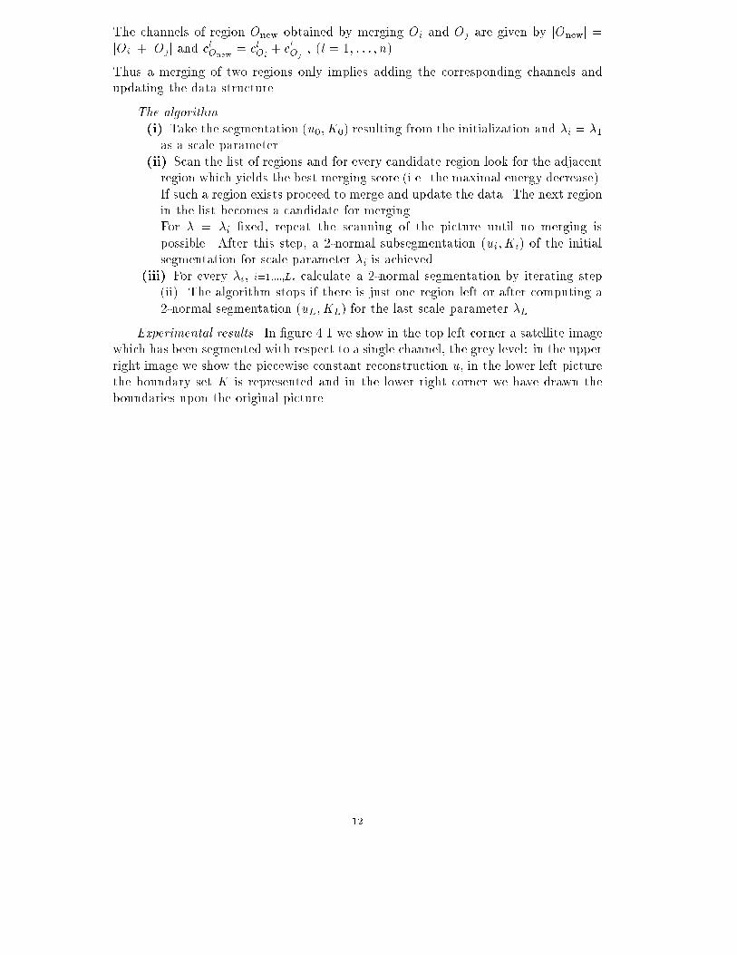
The channels of region Onew obtained by merging Oi and Oj are given by jOnewj =jOij+ jOjj and clOnew = clOi + clOj ; (l = 1; : : : ; n).Thus a merging of two regions only implies adding the corresponding channels andupdating the data structure.The algorithm.(i) Take the segmentation (u0; K0) resulting from the initialization and �i = �1as a scale parameter.(ii) Scan the list of regions and for every candidate region look for the adjacentregion which yields the best merging score (i.e. the maximal energy decrease).If such a region exists proceed to merge and update the data. The next regionin the list becomes a candidate for merging.For � = �i �xed, repeat the scanning of the picture until no merging ispossible. After this step, a 2-normal subsegmentation (ui; Ki) of the initialsegmentation for scale parameter �i is achieved.(iii) For every �i, i=1;:::;L, calculate a 2-normal segmentation by iterating step(ii). The algorithm stops if there is just one region left or after computing a2-normal segmentation (uL; KL) for the last scale parameter �L.Experimental results. In �gure 4.1 we show in the top left corner a satellite imagewhich has been segmented with respect to a single channel, the grey level: in the upperright image we show the piecewise constant reconstruction u, in the lower left picturethe boundary set K is represented and in the lower right corner we have drawn theboundaries upon the original picture.

12

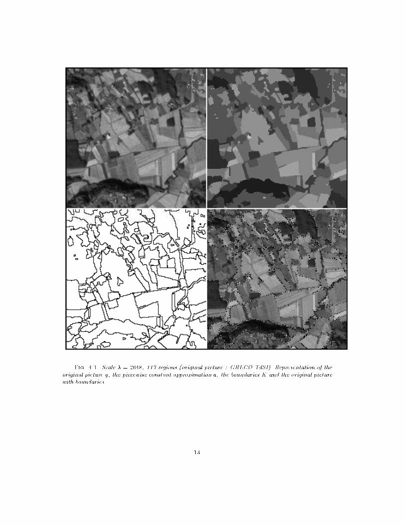
Fig. 4.1. Scale � = 2048, 117 regions (original picture : GRECO TdSI). Representation of theoriginal picture g, the piecewise constant approximation u, the boundaries K and the original picturewith boundaries. 13

5. Application to texture discrimination. We follow the ideas of DavidMarr [Marr] concerning the \raw primal sketch". According to this theory the group-ing process of the human visual system should be based on the detection of localfeatures which from the mathematical viewpoint are simply di�erential or semilocalintegrodi�erential operators like the derivatives or convolution by Gaussians. Thepreattentive texture discrimination depends on the fact that at least one of the fea-tures has a bigger or lower local density (see [MaliP2]).It is important to note that most of the channels introduced by the algorithmsof [MaliP2], [VoP], [BovCG], : : : are linear operators which, according to the Wavelettheory, can be computed at each scale in linear time by a pyramidal scheme (alsocalled in this context quadrature mirror �lter [Coh], [EsG]).The wavelet transform allows to compute a multiscale gradient in every directionin linear time (by a quadrature mirror �lter). Since, as recalls David Marr, textures\live independently at di�erent scales", it will be much easier to get discrimination ofmost textures with a fast multiscale analysis. One can for instance use the Daubechies�lters [Daub1, Daub2], which can be computed with quadrature mirror �lters havingvery few coe�cients (eight coe�cients are enough for a smooth wavelet with two zeromoments). In a work in collaboration with Ja�ard and Journ�e, Daubechies has proveda fast algorithm for a variant of Gabor �ltering ([DaubJJ]). Fast Gabor �ltering mayalso provide cheap channels for our segmentation algorithm, which prove very usefulfor almost periodic textures.Note however that the human eye is by no means perfect in texture discriminationand that it can reasonably be argued that a discrimination algorithm could be moreaccurate and discriminate textures which are not directly accessible to the human eye.In our opinion, a successful computational model of texture discrimination should dobetter than the human eye in some cases, and therefore be used as an enhancementoperator (see �gure 5.3).Let us summarize the assumptions on which we base our segmentation algorithm :� We assume, following the theory of Beck and Julesz (see [Bec, Ju]) and somerecent experimental and computational con�rmation of it [BovCG, MaliP2,VoP] that a reasonable number of channels de�ned on the image is enough inorder that for any pair of preattentively di�erent textures, at least one of thechannels will help to discriminate them.� We are not able now to say which channels are necessary or su�cient in orderto get a discrimination similar to that of the human eye. Now, our universalsegmentation algorithm is designed for fast speci�c applications, but also as afast and robust experimental device allowing progress in the question of whichchannels are necessary in order to match the human visual performance.Examples. Let g = (g1; : : : ; gn) be the initial data calculated from the picture~g and u = (u1; : : : ; un) the piecewise constant estimate ( it turns out that ui is themean value of gi on each connected component). Using the functionalZ ku� gk2pond: + � � `(K) ;where k:kpond: is a weighted norm, we calculate a 2-normal segmentation.The initial datum g for the experiments related below is given in our experiments by14

an oversampled Haar-Wavelet transform of the picture ~g. More precisely the image isconvloved with a bank of linear �lters Fk, followed by half-wave recti�cation.R2k = (~g ? Fk)+ (x; y) ; R2k+1 = (~g ? Fk)� (x; y)It should be noticed that all the �lters Fk are of zero mean and separable:H1a(x; y) = �[�a;a](x) ��[0;a](y)� �[�a;o](y)�H2a(x; y) = �[�a;a](y) ��[0;a](x)� �[�a:0](x)�H3a(x; y) = ��[0;a](x)� �[�a;o](x)���[0;a](y)� �[�a;o](y)�where � is the caracteristic function on IR and a = 2j , 1 � j � J , J is the decompo-sition order of the analysis.The Ris are then �ltered by Gaussians in order to obtain texton densities. The size ofthese Gaussians corresponds to the \�-neighbourhoods" of Julesz. Let us recall thede�nition of Julesz [Ju]: \ The �-neighbourhood is the area, in which di�erences intexton densities are determined. Textons are formed only if the adjacent elements liewithin the �-neighborhood."Finally we obtain the gis, the components of our initial datum g, as the �ltered versionsof the Ri channels.The aim of our experiences is to get a veri�cation of the Julesz doctrine : we stopour region growing if the desired number of regions is reached ( e.g. if there are twotextures we proceed until we have a partition in two regions of our image) . If thediscrimination is successful ( i.e the two regions correspond to the textures' location)one can say that the used channels are able to discriminate the given textures ( it isimportant to notice that we don't use the grey-channel information ).The experimentations used Brodatz pictures (see [Bro]) and a synthetic image whichillustrates the need to keep all the channel involved in the discrimination process.6. Conclusion. We have proved that the minimizing of the \simplest" segmenta-tion energy entails the implicit realization of properties sought by most segmentationdevices. Indeed, the most primitive segmentation tool, the \merging", applied tothe simplest possible segmentation energy, is enough to ensure a compact and there-fore small set of possible segmentations, with no small regions and no thin regions.Uniform a priori estimates for the size and number of the regions can be given forall segmentations obtained by exhaustive \merging". Moreover, the region growingmethod associated with the recursive merging is enough to retrieve all piecewise con-stant functions. Such a merging method is not accurate enough to obtain smoothboundaries, but it controls anyway their length. The big advantage of this method isits velocity.Aknowledgment: We thank Yves Meyer, Pietro Perona and Lenny Rudin for valuableconversations and remarks. 15

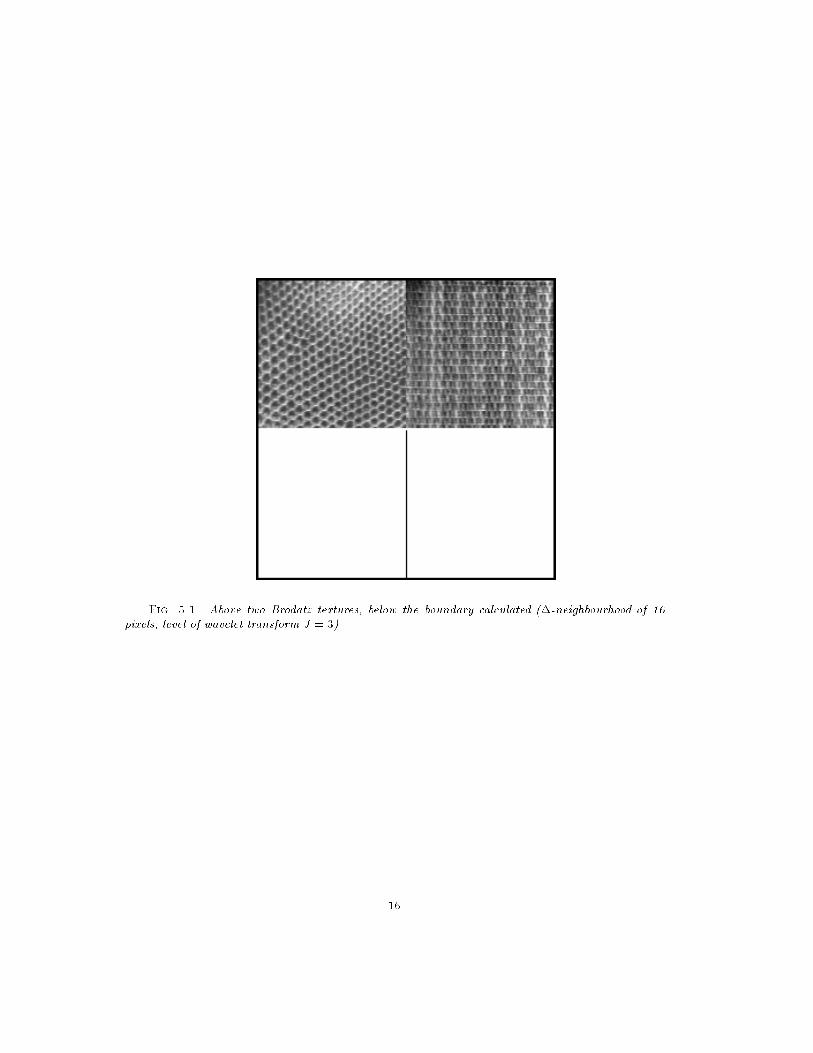
Fig. 5.1. Above two Brodatz textures, below the boundary calculated (�-neighbourhood of 16pixels, level of wavelet transform J = 3) .16

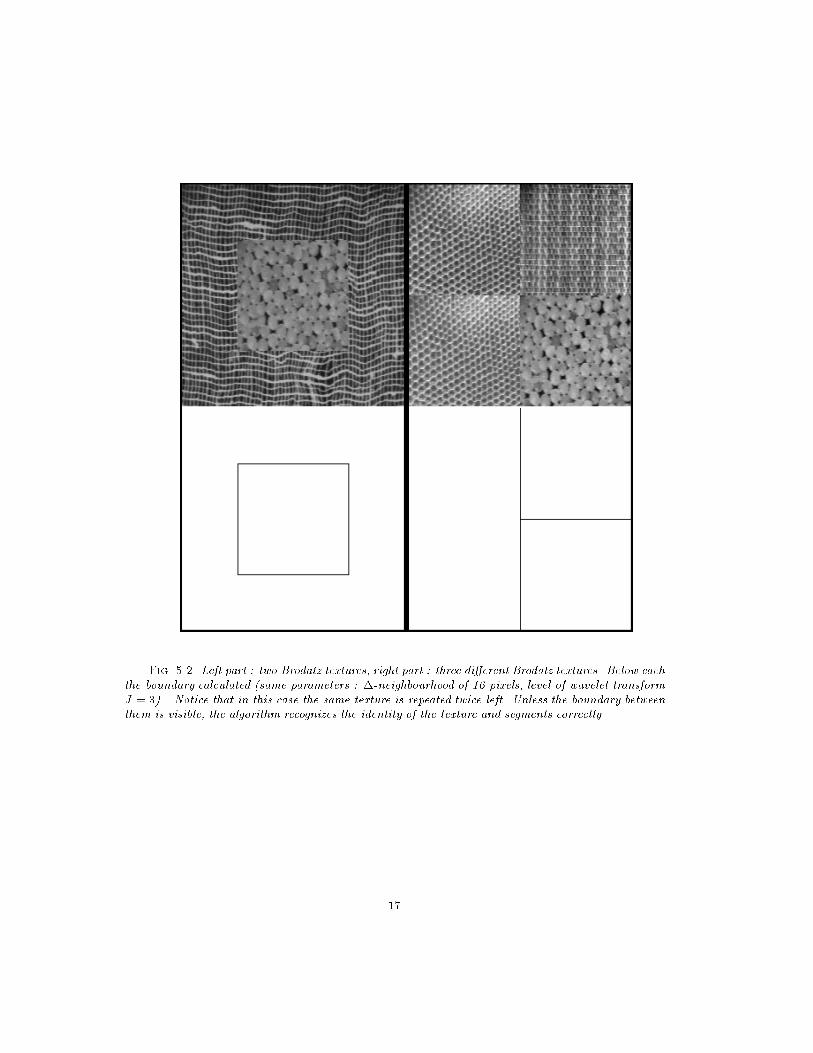
Fig. 5.2. Left part : two Brodatz textures, right part : three di�erent Brodatz textures. Below eachthe boundary calculated (same parameters : �-neighbourhood of 16 pixels, level of wavelet transformJ = 3) . Notice that in this case the same texture is repeated twice left. Unless the boundary betweenthem is visible, the algorithm recognizes the identity of the texture and segments correctly.17

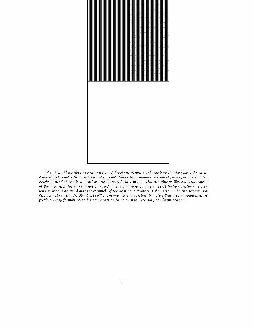
Fig. 5.3. Above the textures : on the left hand one dominant channel; on the right hand the samedominant channel with a weak second channel. Below the boundary calculated (same parameters: �-neighbourhood of 16 pixels, level of wavelet transform J = 3) . This experiment illustrates the powerof the algorithm for discrimination based on nondominant channels. Most texture analysis devicestend to base it on the dominant channel. If the dominant channel is the same in the two regions, nodiscrimination [BovCG,MaliP2,Vop2] is possible. It is important to notice that a variational methodyields an easy formalization for segmentation based on non-necessary dominant channel.18

REFERENCES[Ale] P.S. Aleksandrov. Combinatorial Topology. Vol. 1, chap. 2, Graylock Press NY, 1956.[Amb] L. Ambrosio. A compactness theorem for a special class of functions of bounded variation.Boll. Un. Mat. Ital. (to appear).[AmbDeG] E. De Giorgi, and L. Ambrosio. Un nuovo tipo di funzionale del calcolo delle variazioni.To appear in Atti Acad. Naz. Lincei Rend. Cl. Sci. Fis. Mat. Natur.[AmbT] L. Ambrosio, and V. M. Tortorelli. Approximation of functionals depending on jumps byelliptic functionals via G-convergence. Preprint. Scuola Normale Superiore di Pisa.[AmiTW] A. Amini, S. Tehrani and T. E. Weymouth. Using dynamic programming for minimizingthe energy of active contours in the presence of hard constraints. Second Interna-tional Conference on Computer Vision (Proceedings of), ICCV'88, IEEE n�883.[Az1] R. Azencott. Synchronous Boltzmann machines and Gibbs �elds; Learning algorithms.To appear, Springer Verlag 1989, (NATO Series, Les Arcs Congress Proceedings).[Az2] R. Azencott. Boltzmann Machines : high order interactions and synchronous learning.Submitted to IEEE PAMI Trans.[Bec] J. Beck. Organization and representation in perception. Chapter in Textural se gmenta-tion, Erlbaum, Hillsdale, NJ, 1982.[BecSI] J. Beck, A. Sutter and R. Ivry. Spatial frequency channels and perceptual grouping intexture segregation. Computer Vision, Graphics and Image Processing, 37, 299-325,1987.[BlakZ] A. Blake and A. Zisserman. Visual Reconstruction.MIT Press, 1987.[BlatM] J. Blat, and JM. Morel. Elliptic problems in image segmentation and their relation tofracture theory. Proceedings of the Int. Conf. on nonlinear elliptic and parabolicproblems, Nancy 88 (Longman 89).[BovCG] A.C. Bovik, M. Clark and W. S. Geisler. Computational texture analysis using localizedspatial �ltering. IEEE 1987.[Bro] Ph. Brodatz. Textures for artists and designers. Dover Publications Inc. NY 1966.[CarDeGL] M. Carriero, E. DeGiorgi and A. Leaci. Existence theorem for a minimum problem withfree discontinuity set. Arch. Rat. Mech. Anal., vol. 108, 1989.[CarLPP] M. Carriero, D. Leaci, E. Pallara and E. Pascali. Euler conditions for a minimum prob-lem with discontinuity surfaces. Preprint Universita degli studi di Lecce (Italy)[Coh] A. Cohen. Ondelettes, analyses multir�esolutions et �ltres miroir en quadrature. Ann.Inst. Henri Poincar�e, Analyse non lin�eaire, Vol. 7, n�5, p.439-459, 1990.[CohDF] A. Cohen, I. Daubechies and J.C. Feauveau. Biorthogonal bases of compactly supportedwavelets. Preprint Bell Labs, 1989.[CongT] G. Congedo and I. Tamanini. On the existence of solutions to a problem in image seg-mentation. Preprint, Dipartimento di Matematica, Univ. di Trento, 38050 Italy.[DalMMS1] G. Dal Maso, J.M. Morel and S. Solimini. Une approche variationnelle en traitementd'images : r�esultats d'existence et d'approximation. C.R. Acad. Sci. Paris, t.308,S�erie I, p. 549-554, 1989.[DalMMS2] G. Dal Maso, J.M. Morel and S. Solimini. A variational method in image segmentation:existence and approximation results. Acta Matematica Vol. 168, 1992.[Daub1] I. Daubechies. Orthonormal bases of compactly supported wavelets. Comm. Pure andApplied Math., vol. 41, p.909-996, 1988.[Daub2] I. Daubechies. Orthonormal bases of compactly supported wavelets. Part II, II, PreprintBell Labs, 1989.[DaubJJ] I. Daubechies, S. Ja�ard and J.L. Journ�e. A simple Wilson orthonormal basis withexponential decay. Preprint Bell Labs, 1989.[DeG] E. De Giorgi. Free discontinuity problems in calculus of variations. To appear, Proc. ofthe meeting in J.L. Lions's honour, Paris, 1988.[DeGCL] E. DeGiorgi, M. Carriero and A. Leaci. Existence theorem for a minimum problem withfree discontinuity set. Arch.Rat.Mech.Anal., Vol.108, 1988, p.195-218.[DibK] F. Dibos and G. Koep er. Propri�et�e de r�egularit�e des contours d'une image segment�ee.C.R. Acad. Sci. Paris, t. 313, S�erie I, p. 573-578, 1991.[EsG] D. Esteban and C. Galand. Application of QMF to split-band voice coding schemes.Proc. of Int. Conf. Acoust. Speech, Signal Processing, Harford, 1977.[Fed] H. Federer. Geometric Measure Theory. Springer-Verlag,1969.[FoT] I. Fonseca and L. Tartar. The gradient theory of phase transitions for systems with two19

potential wells. Carnegie Mellon Univ. To appear.[FroM] J. Froment and J.M. Morel. Analyse multi�echelle, vision st�er�eo et ondelettes. Expos�en�5 du S�eminaire d'Orsay \Les ondelettes en 89", ed. P.G. Lemari�e, Springer Verlag1990.[GemG] S. Geman and D. Geman. Stochastic relaxation, Gibbs distributions and the Baysianrestoration of images. IEEE PAMI 6, 1984.[HarS] R.M. Haralick and L.G. Shapiro. Image segmentation techniques. Computer VisionGraphics and Image Processing, 29, 100-132, 1985.[Ju] B. Julesz. Texton gradients : the texton theory revisited. Biological Cybernetics, 54 :245-251, 1986.[KasWT] M. Kass, A. Witkin and D. Terzopoulos. Snakes: active contour models. 1stInt.Comp.Vis.Conf. 1987, IEEE n�777.[KoeMS] G. Koep er, J.M. Morel and S. Solimini. Segmentation by minimizing a functional andthe \merging" methods. Proceedings `GRETSI Colloque' in Juan-les-Pins, Septem-ber 1991 (France).[MaliP1] J. Malik and P. Perona A scale space and edge detection using anisotropic di�usion.Proc. IEEE Computer Soc. Workshop on Computer Vision, 1987.[MaliP2] J. Malik and P. Perona. Preattentive texture discrimination with early vision mecha-nisms. Journ. of the Opt. Society. of America. A, 923-932, vol. 7, n�5, 1991.[Mall] S.Mallat. A theory for multiresolution signal decomposition: the wavelet representation.IEEE Trans. on Pattern Analysis and Machine Intelligence, 674-693, July 1989.[Marr] D. Marr. Vision. Freeman and Co. 1982.[Me] Y. Meyer. Ondelettes, fonctions splines et analyses gradu�ees. Rapport CEREMADEn�8703, 1987.[MorS1] J.M. Morel and S. Solimini. Segmentation of images by variational methods: a construc-tive approach. Rev. Matematica de la Universidad Complutense de Madrid, Vol.1,n�1,2,3, 169-182, 1988.[MorS2] JM. Morel and S. Solimini. Segmentation d'images par m�ethode variationnelle : unepreuve constructive d'existence. C. R. Acad. Sci. Paris S�erie I, 1988.[MumS1] D. Mumford and J. Shah. Optimal Approximations by Piecewise Smooth Functions andAssociated Variational Problems. Communications on Pure and Applied Mathemat-ics. vol. XLII No.4, 1989.[MumS2] D. Mumford and J. Shah. Boundary detection by minimizing functionals. Image Under-standing, 1988, Ed. S. Ullman and W. Richards.[PapJ] N.T. Pappas and N.S. Jayant. An adaptive clustering algorithm for image segmentation.Proc. of ICCV'88, IEEE n� 883, 310-315, 1988.[Pav1] T. Pavlidis. Segmentation of pictures and maps through functional approximation.Comp.Gr. and Im.Proc. 1, 360-372, 1972.[Pav2] T. Pavlidis. Structural Pattern Recognition. Springer, New York 1977.[PavL] T. Pavlidis and Y.T. Liow. Integrating Region Growing and Edge Detection. Proc. ofthe IEEE Conf. Comp. Vision and Patt. Recognition 1988.[Ric] T.J. Richardson. Scale independant piecewise smooth segmentation of images via vari-ational methods. PhD. Dissertation, Lab. for Information and Decision Systems,MIT, Cambridge MA 02139, February 1990.[Si-L] L. Simon. Lectures on Geometric Measure Theory.Centre for Math. Analysis. AustralianNat. Univ., vol. 33, 1983.[Th] C. Thomassen. The Jordan-Sch�on ies theorem and the classi�cation of surfaces.Am.Math.Monthly, 116-130, February 1992.[VoP] H. Voorhees and T. Poggio. Computing texture boundaries from images. Nature, 333,364-367, 1988.[Zu] S.W. Zucker. Region growing: Childhood and Adolescence (Survey). Comp. Graphicsand Image Proc. 5, 382-399, 1976.20