Utility of SCaMPR Satellite versus Ground-Based Quantitative Precipitation Estimatesin Operational Flood Forecasting: The Effects of TRMM Data Ingest

HAKSU LEE,*,1 YU ZHANG,# DONG-JUN SEO,*,@ ROBERT J. KULIGOWSKI,&

DAVID KITZMILLER,# AND ROBERT CORBY**

* NOAA/National Weather Service/Office of Hydrologic Development, Silver Spring, Maryland, and University

Corporation for Atmospheric Research, Boulder, Colorado#NOAA/National Weather Service/Office of Hydrologic Development, Silver Spring, Maryland

&NOAA/National Environmental Satellite, Data and Information Service/Center for Satellite Applications

and Research, College Park, Maryland

** NOAA/National Weather Service/West Gulf River Forecast Center, Fort Worth, Texas

(Manuscript received 17 October 2012, in final form 13 December 2013)

ABSTRACT

This study examines the utility of satellite-based quantitative precipitation estimates (QPEs) from the Self-

CalibratingMultivariate PrecipitationRetrieval (SCaMPR) algorithm for hydrologic prediction. In this work,

two sets of SCaMPRQPEs, onewithout and the other with Tropical RainfallMeasurementMission (TRMM)

version 6 data integrated, were used as input forcing to the lumped National Weather Service hydrologic

model to retrospectively generate flow simulations for 10 Texas catchments over 2000–07. The year 2000 was

used for the model spinup, 2001–04 for calibration, and 2005–07 for validation. The results were validated

using observed streamflow alongside similar simulations obtained using interpolated gauge QPEs with

varying gauge network densities, and still others using the operational radar–gauge multisensor product

(MAPX). The focus of the evaluation was on the high-flow events. A number of factors that could impact

the relative utility of SCaMPR satellite QPE and gauge-only analysis (GMOSAIC) for flood prediction

were examined, namely, 1) the incremental impacts of TRMM version 6 data ingest, 2) gauge density, 3)

effects of calibration approaches, and 4) basin properties. Results indicate that ground-sensor-based QPEs

in a broad sense outperform SCaMPR QPEs, while SCaMPR QPEs are competitive in a minority of

catchments. TRMM ingest helped substantially improve the SCaMPR QPE–based simulation results.

Change in calibration forcing, that is, calibrating the model using individual QPEs rather than the MAPX

(the most accurate QPE), yielded overall improvements to the simulation accuracy but did not change the

relative performance of the QPEs.

1. Introduction

Precipitation is a crucial hydrometeorological input

for hydrologic models to produce skilful flood pre-

diction. At most U.S. River Forecast Centers (RFCs),

the radar–gauge multisensor quantitative precipitation

estimate (QPE), or MQPE hereinafter, serves as input

data to the Sacramento SoilMoistureAccountingmodel

(SAC-SMA) (Burnash et al. 1973) to support flood fore-

casting on a daily basis. MQPEs are produced by merging

radar and gauge data via the multisensor precipitation

estimator (MPE) (Fulton et al. 1998; Seo 1998a,b; Seo

et al. 1999; Seo and Breidenbach 2002); in operations,

a basin average of gridded MQPEs, or radar–gauge

multisensor product (MAPX), is often used. In the

United States, the radar and gauge networks are un-

evenly distributed, leavingmany areas without adequate

coverage. In view of this fact and the presence of errors

associated with rain gauges and radar (Zhang et al.

2013), it is widely anticipated that the use of satellite

QPEs (SQPEs) could augment operational river flow

forecasting for some basins outside of radar coverage

and in sparsely gauged areas. They will need to be used

1Current affiliation: NOAA/National Weather Service/Office

of Climate, Water, andWeather Services, Silver Spring, Maryland.@Current affiliation: Department of Civil Engineering, Univer-

sity of Texas at Arlington, Arlington, Texas.

Corresponding author address: Haksu Lee, NOAA/NWS/Office

of Climate, Water, and Weather Services, 1325 East–West High-

way, Silver Spring, MD 20910.

E-mail: haksu.lee@noaa.gov

JUNE 2014 LEE ET AL . 1051

DOI: 10.1175/JHM-D-12-0151.1

in a manner that considers their own limitations, of

course, including complex terrain (orographic enhance-

ments of convection are captured, but seeder–feeder

enhancements are not) and snow cover [which precludes

microwave (MW)-based retrievals but still allows in-

frared (IR)-based estimates].

Among real-time multisatellite QPE algorithms, this

study uses the Self-Calibrating Multivariate Precip-

itation Retrieval (SCaMPR) (Kuligowski 2002, 2010;

Kuligowski et al. 2013) because of its short latency

(;17min) relative to other multisatellite QPE algo-

rithms such as the Climate Prediction Center (CPC)

morphing technique (CMORPH) (Joyce et al. 2004),

Precipitation Estimation from Remotely Sensed Infor-

mation using Artificial Neural Networks (PERSIANN)

(Sorooshian et al. 2000) and PERSIANN Cloud Clas-

sification System (PERSIANN-CCS) (Hong et al. 2004),

Global Satellite Mapping of Precipitation (GSMaP)

near real time (GSMaP-NRT) (Kubota et al. 2007), the

Naval Research Laboratory (NRL) blended product

(Turk and Miller 2005), and the Tropical Rainfall

Measuring Mission (TRMM) Multisatellite Precip-

itation Analysis (TMPA) (Huffman et al. 2007, 2010).

This feature renders the SCaMPR SQPE more suitable

for real-time forecasting of flash and river floods than

other SQPEs. In light of the NWS efforts to capitalize on

SQPE from the future Global Precipitation Measure-

ment (GPM) satellite, we evaluated two SCaMPR

SQPEs in this study: SCaMPR-P (P for passive micro-

wave), which uses Special Sensor Microwave Imager

(SSM/I) and Advanced Microwave Sounding Unit

(AMSU)-B data as calibration targets, and SCaMPR-T

(T for TRMM), which adds predictands from the TRMM

version 6 algorithms using the TRMM Microwave Im-

ager (TMI) and Precipitation Radar (TPR). These

TRMM instruments provide proxies of similar products

from GPM Microwave Imager and Dual-Frequency

Precipitation Radar (DPR).

The comparative utility of gauge-, radar-, and satellite-

based QPEs for hydrological applications has been ex-

tensively studied in hydrology and hydrometeorology.

Compared to mean-field bias-adjusted radar or multi-

sensor QPEs, gauge rainfall and local bias-adjusted ra-

dar or multisensor QPEs may provide limited information

on rainfall spatial variability, resulting in reduced perfor-

mance in streamflow simulation (Gourley and Vieux

2005). Adjusting radar rainfall to account for errors as-

sociated with the vertical profile of reflectivity (VPR),

reflectivity–rainfall rate (Z–R) relationship, and radar

calibration can significantly improve streamflow simu-

lations using hydrologic models (Borga 2002); in a simi-

lar vein, accounting for sources of bias in satellite estimates

such as topography, climate regime, land use, and land

cover may also enhance their utility in hydrologic fore-

casting (Gebregiorgis and Hossain 2012; Gebregiorgis

et al. 2012). When compared to IR-based satellite rain-

fall retrievals, passive microwave (PM) retrievals were

found to overestimate time to peak flow, especially for

flood events with short duration (Hossain andAnagnostou

2004). Compared to PM retrievals, combined PM–IR

retrievals degraded the performance of a hydrologic

model on flood volume and time to peak owing to the

lower rain detection accuracy of the IR retrievals (Hossain

and Anagnostou 2004). Bitew and Gebremichael (2011a)

reported that algorithms directly using MW data

(CMORPH, TMPA 3B42RT) outperformed an algo-

rithm fitting IR data to MW rain rates (PERSIANN),

and that SQPE (TMPA 3B42RT) performed much

better than the satellite-gauge QPE (TMPA 3B42). Su

et al. (2008) demonstrated that variable infiltration ca-

pacity (VIC) model simulations for the La Plata basin

(3.2 3 106 km2) using TMPA SQPE reproduced flood

events well on a daily scale, as well as seasonal and in-

terannual streamflow variability. However, simulated

daily peak flows using TMPA SQPE tended to be biased

high (Su et al. 2008). While much of this bias can be

addressed by incorporating rain gauge data into the

analysis (e.g., Behrangi et al. 2011; Pan et al. 2010), this

presumes the availability of such data in sufficient

quantity, quality, and timeliness in real-time operational

applications, which is infrequently the case. Further-

more, gauge correction is just as critical for hydrologic

applications of radar data, as pointed out by Gourley

et al. (2011).

Although the aforementioned literature provides a

broad view of the quality of various satellite and com-

posite QPE products and their implications on hydro-

logic modeling, few of them were able to address two

important science questions: 1) under what specific cir-

cumstances (e.g., the density of the gauge network)

might the value of the SQPEs exceed that of simple,

gauge-interpolated QPEs and 2) what is the actual im-

pact of TRMM and potentially GPM data alone on the

hydrologic prediction accuracy? The isolated impacts of

TRMM data were not examined in these studies, as the

work relied on blended products fromTRMMand other

satellites (Bitew and Gebremichael 2011b; Su et al.

2008). This study is a unique opportunity to address both

questions. To answer the first question, a high-quality

radar–gauge QPE (MQPE) and multiple sets of gauge-

only analyses based on thinned gauge networks are

employed, and the results are contrasted to those from

the SCaMPR QPEs. The second question is addressed

by using the two sets of SCaMPR QPEs, one with and

the other without TRMM ingest. Such an experimental

design allows us to isolate the impacts of TRMM QPEs

1052 JOURNAL OF HYDROMETEOROLOGY VOLUME 15

on hydrologic prediction and thereby help anticipate the

potential hydrologic value of similar QPEs from GPM.

It is worth noting that, since TRMM is not in a sun-

synchronous orbit, its expected impacts will vary with

time as it samples different portions of the diurnal

convective cycle. These effects should largely average

out during a multiyear study such as this one and thus

should not materially affect the conclusions reached

here; however, the shorter-term impacts of orbital dy-

namics on the rainfall retrievals would certainly cause

some fluctuations in error with time and would be an

interesting avenue for future study.

Other distinct features of this study include the fol-

lowing. First, this study employs the lumped NWS

hydrologic model, which, despite not being a fully

physically basedmodel, has been shown to be among the

best performers during the two Distributed Model In-

tercomparison Project (DMIP) experiments (Reed et al.

2004; Smith et al. 2012). Using this model not only helps

reduce the impact of model inaccuracy, but also allows

the experiment to mimic operational hydrologic pre-

diction at NWS. Second, a careful calibration/validation

experiment was carried out wherein calibration was

done via an objective, automated approach that has been

shown to work effectively (Kuzmin et al. 2008). Third, in

contrast to studies, including Bitew and Gebremichael

(2011a) and Su et al. (2008), presenting hydrologic ap-

plications of SQPEs for daily streamflow simulations, the

study focuses on hourly streamflow simulation and exam-

ines the accuracy of the model in representing high flow

events (near or exceeding flood stage) rather than average

flow conditions; therefore, the result has more direct im-

plications for potential operational adoption of SCaMPR

QPEs. Fourth, the study is based on a considerably larger

sample, which encompasses 10 catchments with a variety of

size and hydroclimate regimes, and thereby allows a close

examination of the dependence of hydrologic fidelity of

SCaMPR on these features.

This paper is organized as follows. Section 2 describes

the hydrological model, parameter estimation and cali-

bration procedure, and validation metrics. Section 3

describes the study basins and QPEs. Section 4 sum-

marizes theQPE evaluation results and discussion of the

model performance on simulating flood events. Finally,

section 5 presents conclusions.

2. Hydrological model, parameter estimation andcalibration procedure, and evaluation metrics

a. Hydrological model

The model used in this study is the lumped Sacra-

mento Soil Moisture Accounting model (Burnash et al.

1973) operating on an hourly time step. While SAC-

SMA conceptualizes rainfall–runoff transformation

processes focused on parameterizing soil moisture char-

acteristics, its parameters were developed in a way to be

interpreted with a physical meaning. Since its first in-

troduction, the SAC-SMA has been used extensively in

operations and in scientific studies ranging from flash

flood modeling (Reed et al. 2007) to land surface mod-

eling (Schaake et al. 2001) to data assimilation (Seo et al.

2009) to ensemble forecasting (Seo et al. 2010). The SAC-

SMA is available within the Community Hydrologic

Prediction System (CHPS) of the NWS and has been

used inmost RFCs to issue flood forecasts on a daily basis

throughout the United States. The SAC-SMA inputs are

mean areal precipitation (MAP) and monthly climatol-

ogy of daily mean areal potential evapotranspiration

(MAPE), and the output is the total channel inflow (TCI)

from two subsurface soil storages—upper zone (UZ) and

lower zone (LZ)—plus the overland flow zone. The LZ is

normally much thicker than the UZ and contains the

majority of soil moisture to meet the evapotranspiration

demand. In addition, the LZ is the primary source of

baseflow fed to the channel. In the UZ, soil moisture is

divided into tension and free water content, or UZTWC

and UZFWC, respectively. Similarly, the LZ soil mois-

ture states are composed of tension water (LZTWC) and

supplemental and primary free water (LZFSC and

LZFPC, respectively). Water stored in the impervious

surface area and five soil moisture content values in two

subsurface storages interact to generate six runoff com-

ponents: impervious, surface, and direct runoff as fast-

response components and interflow, supplemental, and

primary groundwater runoff as slow-response compo-

nents (Koren et al. 2004). The TCI from the SAC-SMA is

then routed through a unit hydrograph (UH) to obtain

streamflow at the outlet of a basin.

b. Parameter estimation and calibration procedure

In the first step, the Adjoint-Based Optimizer

(AB_OPT) (Seo et al. 2009) is used to estimate long-term

biases in the precipitation and potential evaporation (PE)

data, which is followed by estimating the empirical UH.

In the last step of AB_OPT, the SAC-SMA model pa-

rameters are locally calibrated. The AB_OPT uses ob-

served streamflow as a calibration target at all three steps

but calibrates different parameters at each step.

The long-term biases in the precipitation and PE data

are estimated based on the water balance concept, and

this estimate of long-term bias in each QPE product is

used to correct the QPE product. Equation (1) is the

objective function (JB) used in this step where the control

variables include multiplicative adjustment factors for

precipitation (XP) and potential evaporation data (XE):

JUNE 2014 LEE ET AL . 1053

JB5

��n

i51

ZQ,i 2 �n

i51

HQ,i(XP,XE)

�2(1)

subject to

XS,j5M(XS,j21,XP,XE), j5 2, . . . ,n , (2)

XminS,j #XS,j#Xmax

S,j , j5 1, . . . ,n . (3)

In the above, ZQ,i is the observed streamflow at hour

i (m3 s21); HQ,i(�,�) is the mapping of the control vari-

ables to the simulated flow at hour i;M(�,�,�) is themodel

that calculates the SAC states at hour j (XS,j) based on

model dynamics and the SAC states in the previous time

step (XS,j21); n denotes the total number of hours in the

simulation period. To capture the total volume of

streamflow observations (ZQ,i) for the entire calibration

period, the bias in the PE data is adjusted during the

procedure along with the bias in the precipitation data.

In this step, the numerical algorithm used is the Broyden–

Fletcher–Goldfarb–Shanno variant of Davidon–Fletcher–

Powell minimization (DFPMIN) (Press et al. 1992).

Equation (4) shows the objective function (JUH) for

the empirical UH estimation with the DFPMIN algo-

rithm. In Eq. (4), the control variables are UH ordinates

(XUH).

JUH 5 �n

i51

[ZQ,i 2HQ,i(XUH)]2 (4)

subject to

XUH,j $ 0, j5 1, . . . , ny . (5)

In the above, XUH,j is the jth ordinate of the UH

(m3 s21 mm21) and ny denotes the total number of UH

ordinates.

The local optimization of the SAC model parameters

is implemented with the stepwise line search (SLS)

technique (Kuzmin et al. 2008). Equation (6) shows the

objective function (JPAR) where the control variables

are the SAC parameters (XPAR):

JPAR5

ffiffiffiffiffiffiffiffiffiffiffiffiffiffiffiffiffiffiffiffiffiffiffiffiffiffiffiffiffiffiffiffiffiffiffiffiffiffiffiffiffiffiffiffiffiffiffiffiffiffiffiffiffiffiffiffiffiffiffiffiffiffiffiffiffiffiffiffiffiffiffiffiffiffiffiffiffiffiffi�K

k51

�s1

sk

�2

�nk

i51

[ZQ,k,i 2HQ,k,i(XPAR)]2

s(6)

subject to

XS,k 5M(XS,k21,XPAR), (7)

XminS,j #XS,j#Xmax

S,j , j5 1, . . . ,n , (8)

XminPAR,j #XPAR,j #Xmax

PAR,j, j5 1, . . . ,m . (9)

In Eqs. (6)–(9), ZQ,k,i and HQ,k,i(�) denote the observed

and simulated flows (m3 s21), respectively, which were

averaged over time interval k at the kth time scale; sk

the standard deviation of observed flow at the kth time

scale; K the total number of time scales; nk the number

of observations at the kth time scale;XPAR the vector of

the SAC parameters; XPAR,jmin and XPAR,j

max denote the

lower and upper bounds of the jth SAC parameter; and

m the total number of SAC parameters. In this work, we

used k5 1, 2, 3, and 4, which correspond to hourly, daily,

weekly, and monthly scales of aggregation.

c. Evaluation metrics

Evaluation metrics used in this study include proba-

bility of detection (POD) (Wilks 2006), false alarm rate

(FAR) (Wilks 2006), Heidke skill score (HSS) (Doswell

et al. 1990), mean absolute peak flow error (EP), mean

absolute peak time error (ET), weighted mean absolute

peak flow error (WEP), weighted mean absolute peak

time error (WET), and rms error (RMSE). POD, FAR,

HSS,EP,ET,WEP, andWET are defined inEqs. (10)–(16):

POD(QT)5x

x1 y, (10)

FAR(QT)5z

x1 z, (11)

HSS(QT)52(xw2 yz)

y21 z21 2xw1 (y1 z)(x1w), (12)

EP 51

N�N

i51

jQPi2QPsij , (13)

ET 51

N�N

i51

jTPi2TPsij , (14)

WEP 51

N�N

i51

1

QPi

jQPi 2QPsij , (15)

WET 51

N�N

i51

1

tPjTPi2TPsij , (16)

where x is the number of correctly detected flow events

(QO $ QT, QS $ QT); y the number of missed events

(QO $ QT, QS , QT); z is the number of false alarms

(QO , QT, QS $ QT); and w is the number of correctly

detected nonevents (QO , QT, QS , QT). QO, QS, and

QT denote observed flow, simulated flow, and threshold

discharge, respectively; QPi, and QPsi represent the ob-

served and simulated peak discharge of the ith flood

1054 JOURNAL OF HYDROMETEOROLOGY VOLUME 15

event, respectively; TPi and TPsi represent the observed

and simulated time to the ith peak, respectively; tP de-

notes time to peak flow of the empirical unit hydrograph

estimated using MAPX (Table 1); N denotes the num-

ber of flood events selected.

As noted by Doswell et al. (1990), HSS falls within

a (21, 1) range: HSS5 1 without any incorrect forecasts,

that is, y 5 z 5 0; HSS 5 0 if x 5 y 5 0 (no observed

events) or x 5 z 5 0 (no events forecast); HSS 5 22zy/

(y2 1 z2) if x 5 w 5 0 (no correct forecasts). In the

evaluation, model skill in detecting flood events is

quantified with POD, FAR, and HSS. Errors in peak

flow magnitude and timing are measured by EP, ET,

WEP, and WET, and overall model performance on

streamflow simulation by RMSE. As EP and ET values

are likely biased toward larger events and/or basins, di-

mensionless measuresWEP andWETwere introduced to

reduce the effect of different sizes of events and basins.

3. Study area and QPE dataset

a. Study basins

The study area includes 10 basins in Texas within the

service area of the West Gulf River Forecast Center

(WGRFC), which range in area from 218 to 1795 km2.

Figure 1 shows the location of the study basins, Hydro-

meteorological Automated Data System (HADS) rain

gauges, and Weather Surveillance Radar-1988 Doppler

(WSR-88D) units (Crum and Alberty 1993). Table 1

summarizes the study basins.

The basins become progressively wetter toward east-

ern Texas in terms of Bowen ratio as well as runoff co-

efficients (Reed et al. 1997). Runoff coefficients vary

from 0.12 to 0.16 for four dry basins in southern Texas

and 0.24 to 0.31 for six wet basins in eastern Texas.Mean

annual MAPX for the period 2000–07 varies from 869 to

1061mm for dry (in terms of Bowen ratio) basins and

831 to 1342mm for wet basins (Table 1). Hourly stream-

flow data were obtained from the U.S. Geological Sur-

vey (USGS). Operational SAC-SMA parameters, 6-h

UH,MAPX, and the monthly climatology ofMAPE are

provided by the WGRFC. The hourly UH is derived

from the operational 6-h UH by the S-curve method

(Chow 1964). Operational SAC-SMA parameters and

hourly UHs are used as a priori input to the calibration

procedure.

b. SCaMPR satellite QPE

SCaMPR is a multisatellite QPE algorithm that aims

to improve the accuracy of IR-based rainfall estimates

from geostationary platforms through calibration against

microwave-based rainfall estimates from low-earth-orbit

platforms (Kuligowski 2002, 2010; Kuligowski et al. 2013).

TABLE 1. Study basins where QW and QF denote flood warning discharge and flood discharge, respectively; CR denotes the runoff

coefficient (annual runoff divided by annual MAPX) for the period of 2000–07; tP is time to peak flow of the empirical unit hydrograph

estimated using MAPX. TheQW andQF for each basin is available on the NWSAdvanced Hydrologic Prediction Service website (http://

water.weather.gov/ahps/).

Basin ID USGS ID Area (km2)

Annual MAPX

(mmyr21)

Annual runoff

(mmyr21) CR QW (m3 s21) QF (m3 s21) tP (h)

GNVT2 08017200 266 911 276 0.3 11 15 17

LYNT2 08110100 519 1006 162 0.16 11 108 18

MCKT2 08058900 439 904 221 0.25 35 45 14

MDST2 08065800 868 1156 305 0.26 88 204 19

MTPT2 08162600 447 1342 380 0.28 23 68 17

QLAT2 08017300 218 831 255 0.31 16 20 14

REFT2 08189500 1795 869 105 0.12 105 140 50

SBMT2 08164300 919 1061 166 0.16 74 125 21

SCDT2 08176900 935 939 111 0.12 127 153 15

SDAT2 08070500 326 1323 320 0.24 48 105 16

FIG. 1. Map of the study basins in Texas and the locations of the

HADS rain gauges and WSR-88D units.

JUNE 2014 LEE ET AL . 1055

The predictors of SCaMPR are IR data (brightness tem-

peratures and derived quantitiess) from the Geostationary

Operational Environmental Satellite (GOES) series. This

study evaluates two SCaMPR products generated with

different predictands. SCaMPR-P (P for passive micro-

wave) was created using only microwave-based rainfall

estimates from the Defense Meteorological Satellite Pro-

gram (DMSP) SSM/I (Ferraro 1997) and the National

Oceanic and Atmospheric Administration (NOAA) Ad-

vancedMicrowaveSoundingUnitB (AMSU-B) (Vila et al.

2007) as predictands. SCaMPR-T (T for TRMM) adds the

TMI (Kummerow et al. 2001) and TPR (Iguchi et al. 2000)

data from the TRMM version 6 algorithms. SCaMPR-T is

included in the evaluation dataset to assess the added

value of TRMM data for operational flood prediction.

Details of the SCaMPR algorithm can be found in

Kuligowski (2002, 2010) and Kuligowski et al. (2013).

c. Gauge-based QPE

Gauge-based QPE is produced by the MPE (Fulton

et al. 1998; Seo et al. 1999; Seo and Breidenbach 2002),

which is a set of algorithms operationally used at the

RFCs and Weather Forecast Offices that has produced

hourly QPE on the Hydrologic Rainfall Analysis and

Prediction (HRAP) grid (;4 3 4 km2, polar stereo-

graphic) over the conterminous United States since

2002. To compute gauge-based QPE, the MPE uses a

single optimal estimation (SOE) algorithm, which is a

variant of simple kriging (Seo 1998a; Journel and

Huijbregts 1978). The gauge rainfall estimates are ad-

justed in reference to climatic precipitation grids from

Parameter-Elevation Regressions on Independent Slopes

Model (PRISM) (Daly et al. 1994) as well as the gauge

reports from the Cooperative Observer Program (COOP)

to improve the overall bias and their spatial pattern

(Zhang et al. 2013). QPE estimated by the MPE algo-

rithm using gauge data only is referred to as GMOSAIC.

The rain gauge data are obtained from the HADS (www.

nws.noaa.gov/oh/hads/; Kim et al. 2009). To address the

effect of gauge density on the utility of GMOSAIC for

flood prediction, seven thinned gauge networks are

randomly drawn using 90%, 50%, and 25%of the gauges in

the original network,which are referred to asGMOSAIC90,

GMOSAIC50, and GMOSAIC25, respectively. One,

two, and four samples are drawn for GMOSAIC90, 50,

and 25, respectively. Table 2 shows the scenario-mean

gauge report frequency (GRF) for GMOSAICs, where

GRF is defined as themean number of gauge reports per

day per HRAP pixel (Zhang et al. 2013).

d. MAPX as a radar–gaugemultisensorQPE (MQPE)

To produce MAPX, radar rainfall is estimated based

on recommendedZ–R relationships in NationalWeather

Service (2006), where Z and R denote the radar re-

flectivity factor and rain rate (mmh21), respectively.

Digital precipitation array (DPA) (Klazura and Imy

1993) products from all WSR-88D sites are then mo-

saicked to produce consolidated radar rainfall. Sub-

sequently, the bias correction of the radar rainfall field is

carried out based on estimated mean field bias (MFB)

(Seo et al. 1999) or local bias (LB) (Seo and Breidenbach

2002) with a reference to the rain gauge data from the

HADS. The MPE optimally combines gauge and bias-

corrected radar rainfall data using a variant of the bi-

variate extension of SOE (Seo 1998a,b), which produces

the gridded MQPE. The gridded MQPE produced by

the automated procedure is subject to scrutiny and de-

cision by forecasters in RFCs. Finally, RFCs produce

MAPX based on the basin average of this gridded

MQPE product. It is worth mentioning that both bias

correction and multisensor merging algorithms in MPE

largely suppress the residual discrepancies among ra-

dars. The MQPEs have been extensively used in hy-

drologic modeling studies as well as field operations

(Seo et al. 2011; Smith et al. 2004, 2012, and references

therein). Previous studies have shown that MQPEs are

comparatively more accurate than simple gauge-only

analysis (Habib et al. 2013; Wang et al. 2008). Habib et al.

(2013) found that rain gauge observations showed lower

skill in rainfall detection than MQPEs. They also found

that the interventions of operational hydrologists improved

the accuracy of MQPEs by reducing the occurrences of

falsely detecting rainfall. Seo (1998b) showed that MQPEs

are generally more accurate than either rain gauge data or

bias-corrected radar rainfall data. Given the findings

from the above studies, we use MAPX as a comparison

standard for both SCaMPR SQPEs and GMOSAICs.

e. Intercomparison of QPEs

Figure 2 shows signature plots of the precipitation

data at hourly and monthly scales. Figure 2a shows the

TABLE 2. Scenario-mean gauge report frequency for

GMOSAIC90, 50, and 25.

Basin

ID

Area

(km2) GMOSAIC90 GMOSAIC50 GMOSAIC25

MCKT2 439 73 40 23

QLAT2 218 70 38 22

GNVT2 266 69 38 21

LYNT2 519 47 25 12

SDAT2 326 40 22 11

SBMT2 919 32 17 9

MDST2 868 31 18 8

MTPT2 447 26 13 7

SCDT2 935 24 14 7

REFT2 1795 13 8 4

1056 JOURNAL OF HYDROMETEOROLOGY VOLUME 15

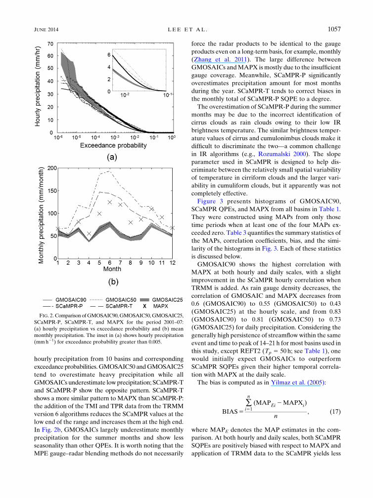
hourly precipitation from 10 basins and corresponding

exceedance probabilities.GMOSAIC50 andGMOSAIC25

tend to overestimate heavy precipitation while all

GMOSAICs underestimate lowprecipitation; SCaMPR-T

and SCaMPR-P show the opposite pattern. SCaMPR-T

shows a more similar pattern to MAPX than SCaMPR-P:

the addition of the TMI and TPR data from the TRMM

version 6 algorithms reduces the SCaMPR values at the

low end of the range and increases them at the high end.

In Fig. 2b, GMOSAICs largely underestimate monthly

precipitation for the summer months and show less

seasonality than other QPEs. It is worth noting that the

MPE gauge–radar blending methods do not necessarily

force the radar products to be identical to the gauge

products even on a long-term basis, for example, monthly

(Zhang et al. 2011). The large difference between

GMOSAICs andMAPX ismostly due to the insufficient

gauge coverage. Meanwhile, SCaMPR-P significantly

overestimates precipitation amount for most months

during the year. SCaMPR-T tends to correct biases in

the monthly total of SCaMPR-P SQPE to a degree.

The overestimation of SCaMPR-P during the summer

months may be due to the incorrect identification of

cirrus clouds as rain clouds owing to their low IR

brightness temperature. The similar brightness temper-

ature values of cirrus and cumulonimbus clouds make it

difficult to discriminate the two—a common challenge

in IR algorithms (e.g., Rozumalski 2000). The slope

parameter used in SCaMPR is designed to help dis-

criminate between the relatively small spatial variability

of temperature in cirriform clouds and the larger vari-

ability in cumuliform clouds, but it apparently was not

completely effective.

Figure 3 presents histograms of GMOSAIC90,

SCaMPR QPEs, and MAPX from all basins in Table 1.

They were constructed using MAPs from only those

time periods when at least one of the four MAPs ex-

ceeded zero. Table 3 quantifies the summary statistics of

the MAPs, correlation coefficients, bias, and the simi-

larity of the histograms in Fig. 3. Each of these statistics

is discussed below.

GMOSAIC90 shows the highest correlation with

MAPX at both hourly and daily scales, with a slight

improvement in the SCaMPR hourly correlation when

TRMM is added. As rain gauge density decreases, the

correlation of GMOSAIC and MAPX decreases from

0.6 (GMOSAIC90) to 0.55 (GMOSAIC50) to 0.43

(GMOSAIC25) at the hourly scale, and from 0.83

(GMOSAIC90) to 0.81 (GMOSAIC50) to 0.73

(GMOSAIC25) for daily precipitation. Considering the

generally high persistence of streamflowwithin the same

event and time to peak of 14–21 h for most basins used in

this study, except REFT2 (Tp 5 50 h; see Table 1), one

would initially expect GMOSAICs to outperform

SCaMPR SQPEs given their higher temporal correla-

tion with MAPX at the daily scale.

The bias is computed as in Yilmaz et al. (2005):

BIAS5

�n

i51

(MAPEi 2MAPXi)

n, (17)

where MAPE denotes the MAP estimates in the com-

parison. At both hourly and daily scales, both SCaMPR

SQPEs are positively biased with respect to MAPX and

application of TRMM data to the SCaMPR yields less

FIG. 2. Comparison ofGMOSAIC90,GMOSAIC50,GMOSAIC25,

SCaMPR-P, SCaMPR-T, and MAPX for the period 2001–07:

(a) hourly precipitation vs exceedance probability and (b) mean

monthly precipitation. The inset in (a) shows hourly precipitation

(mmh21) for exceedance probability greater than 0.005.

JUNE 2014 LEE ET AL . 1057

positively biased SQPE (see also Fig. 2b). On the con-

trary, the GMOSAICs are negatively biased: scenario-

mean bias 5 20.04mmh21 for both GMOSAIC50 and

GMOSAIC25 at the hourly scale (not shown), with

values of 20.89 and 20.99mmday21 for GMOSAIC50

and GMOSAIC25, respectively, at the daily scale (also

not shown).

The similarity in histograms between MAPX and

another QPE is measured by the Kolmogorov–Smirnov

(K–S) statistic (Lampariello 2000; Young 1977). It is

denoted as KSb in Table 3, where the subscript b denotes

the number of bins used to build a histogram:

KSb5 maxx

jFMAPX,b(x)2Fb(x)j . (18)

In the above, FMAPX,b(x) and Fb(x) are sample proba-

bility distribution functions computed from histograms

constructed fromMAPX and anotherQPE, respectively

(Young 1977). The KSb measures the maximum vertical

displacement between the two sample distribution func-

tions. Among GMOSAIC90 and SCaMPR SQPEs,

SCaMPR-T shows the smallest KS10 (i.e., 10 bins) and

KS20 (20 bins) at both hourly and daily scales (Table 3);

this indicates that ingesting TRMM data changes the

distribution of SCaMPR SQPE to be more similar to

that of MAPX.

Another measure of the similarity between histo-

grams is the difference in the mean of the distance be-

tween the sample mean at a bin and the center value of

that bin of a histogram, or Db:

Db 51

n�n

i51

jBi 2Cij21

m�m

i51

jBMAPX,i2Cij , (19)

where Bi denotes the mean of the QPE data in the ith

bin;BMAPX,i is the same asBi, but forMAPX;Ci denotes

the mean of the range used to define the ith bin; n is the

number of bins with more than a single data point; m is

the same as n, but for MAPX. The values of both D10

and D20 at hourly and daily scales are relatively small

compared to the width of each bin, which is 5.4 and

2.7mmh21 in the case of 10 and 20 bins for hourly QPE

and 21.1 and 10.5mmday21 in the case of 10 and 20 bins

for daily QPE, respectively. This indicates that, on the

average, the bin-to-bin mean of GMOSAIC90 and

SCaMPR SQPEs data are highly similar to that for

MAPX despite differences in the number of QPE data

points in each bin. It is also worth noting that theD10 and

D20 values for SCaMPR decrease when TRMM is in-

gested (i.e., the average value of SCaMPR in each bin

decreases), which is consistent with the drying trend in

the bias statistic.

4. Results and discussion

The SAC-SMAmodel simulations are generated with

two sets of model parameters and UH obtained via

FIG. 3. Histograms of MAPs at (a) hourly and (b) daily scale; the

values on the x axis represent the center of the range of values in

each bin.

TABLE 3. Statistics between MAPX and GMOSAIC90 or

SCaMPRSQPEs. In the table,G90, P, andT denoteGMOSAIC90,

SCaMPR-P, and SCaMPR-T, respectively. Similarly to Fig. 3,

histogram-based statistics are calculated using selected MAPs un-

der the condition that one of MAPs at a given time exceeds zero

precipitation. The BIAS, D10, and D20 have the unit of (mmh21) in

the case of hourly MAPs and (mmday21) in the case of daily MAPs.

Statistics

Hourly precipitation Daily precipitation

G90 P T G90 P T

Time series–based statistics

BIAS 20.04 0.04 0.01 20.87 1.05 0.21

CR 0.60 0.52 0.53 0.83 0.70 0.70

Histogram-based statistics

D10 20.05 0.24 20.29 0.63 0.67 0.26

D20 20.03 0.02 20.05 20.004 20.02 20.16

KS10 0.014 0.014 0.004 0.025 0.030 0.006

KS20 0.023 0.037 0.014 0.035 0.039 0.010

1058 JOURNAL OF HYDROMETEOROLOGY VOLUME 15

calibrating the model using either MAPX or the corre-

sponding quantitative precipitation estimate. The use of

MAPX-driven model parameters and UH in the SAC-

SMA model simulations driven by other QPEs may be

justified as follows:MAPX is known to bemore accurate

than most, if not all, other QPEs and serves the opera-

tional reference; hence,MAPX-drivenmodel parameters

and UH may also be considered more representative for

the basin of interest than those derived with any other

QPEs. In this section, we comparatively evaluate the

model performance for simulating flood events for 10

Texas basins, using two sets ofmodel parameters andUH

as well as different QPEs. Flood events are selected using

flood warning discharge (QW) in Table 1 as a threshold;

flood warning discharge (QW) is the precursor of river

conditions evolving to flood stage, requiring proper at-

tentions by operational forecasters. Throughout the

evaluation, the dataset for year 2000 is used for themodel

spinup, 2001–04 for calibration, and 2005–07 for valida-

tion. It is worth mentioning that correcting biases in the

forcing data via AB_OPT [Eqs. (1)–(3)] noticeably im-

proved the long-term bias in simulated flow prior to the

calibration of SAC parameters and UH ordinates [Eqs.

(4)–(9)]. For instance, the multibasin mean of bias in the

flow simulation for the calibration period changed from

0.62 to 0.91 for GMOSAIC90, 1.52 to 0.97 for SCaMPR-P,

0.86 to 0.94 for SCaMPR-T, and 1.19 to 1.09 for MAPX,

where the bias is calculated as the ratio of total simulated

flow for the period of interest to the total observed flow for

the same period. For the validation period, the multibasin

mean bias changed from 0.75 to 1.17 for GMOSAIC90,

1.69 to 1.11 for SCaMPR-P, 1.09 to 0.99 for SCaMPR-T,

and 1.31 to 1.18 for MAPX.

a. Evaluation of flood prediction

The suitability of each QPE for SAC-SMA model

simulations and the relative performance of QPEs are

assessed in terms of the skill in detecting high-flow

events, the error in the simulation of flow magnitude

and timing, and the overall simulation accuracy. To cal-

culate EP, ET, WEP, and WET, we used the observed

flows exceeding flood warning discharge (QW in Table 1).

Calculation of POD, FAR, and HSS includes the period

of time when either observed or simulated flows exceed

QW. The threshold streamflows (QT) used in the calcu-

lation of POD, FAR, and HSS are QW,

2

3QW 1

1

3QF ,

1

3QW 1

2

3QF ,

and QF. Table 4 summarizes the number of events ex-

ceeding floodwarning discharge (QW) or flood discharge

(QF) for the calibration (2001–04) and validation (2005–

07) periods, separately, for each basin.

Overall model performance for flood prediction is

evaluated in terms of multibasin mean (Table 5) and

interbasin variability (Fig. 5) of the statistics used. Table 5

shows statistics averaged over 10 basins, includingMAPX

results as the benchmark. Values in bold denote the QPE

(among SCaMPR SQPEs and GMOSAICs) showing the

best results given the performance measure and calibra-

tion method used. Table 5 can be summarized as follows:

overall, MAPX performs as well as or better than

GMOSAICs and SCaMPR SQPEs for all statistics used.

GMOSAICs generally show a higher POD range than

does SCaMPR SQPE, though the high FAR(QF) of

GMOSAIC25 cancels out the benefit of the high POD

(QF), resulting in lowHSS(QF) for that particular dataset.

Compared to the model simulations using MAPX-

driven parameter and UH, individual QPE calibration

1) generally increases POD(QF) of GMOSAICs,

2) generally decreases FAR(QW) for SCaMPR SQPEs,

3) produces lower RMSE and EP and marginal im-

provement in ET, and 4) generally improves HSS(QF)

for the validation period for both SCaMPR SQPEs and

GMOSAICs. The models with individual QPE calibra-

tion generally outperform the model calibrated using

the most accurate QPE (i.e., MAPX), which is consis-

tent with other studies (e.g., Artan et al. 2007; Bitew and

Gebremichael 2011b; Stisen and Sandholt 2010; Yilmaz

et al. 2005).

The sensitivity of the model performance to the cali-

bration approach is more objectively represented by the

percentage improvement after changing from using

MAPX-driven parameters and UH to the calibration

using corresponding QPEs (Fig. 4). Compared to the

model using MAPX-driven model parameter and UH,

individual QPE calibration generally improves both

GMOSAIC and SCaMPR SQPE results for most sta-

tistics for the validation period, especially HSS(QF).

SCaMPR SQPEs, particularly SCaMPR-P, benefited less

TABLE 4. The number of events exceeding flood warning dis-

charge (NW) and flood discharge (NF) for the calibration and val-

idation periods.

Basin ID

Calibration (2001–04) Validation (2005–07)

NW NF NW NF

GNVT2 28 24 34 28

LYNT2 32 6 24 3

MCKT2 12 8 23 13

MDST2 19 6 14 4

MTPT2 39 15 28 13

QLAT2 26 20 27 20

REFT2 7 4 5 1

SBMT2 22 16 8 5

SCDT2 6 6 3 3

SDAT2 17 3 3 2

JUNE 2014 LEE ET AL . 1059

from individual QPE calibration in terms of POD and

HSS for the calibration period. The multibasin mean

HSS of SCaMPR-P for the calibration period is reduced

by more than 20% after changing the calibration

method (see related discussions at the end of the pre-

vious paragraph).

Figure 5 presents plots of selected quantiles (median

and 25th and 75th quantiles) in two-dimensional space

spanned by two evaluation statistics, characterizing the

interbasin variability of model performance statistics. In

Fig. 5, HSS quantifies the model skill in detecting se-

lected flood events, RMSE shows the overall model

performance for the entire simulation period, POD and

FAR show the skill in correctly or falsely detecting high

flow events at the threshold QW, and WEP and WET

represent errors in the simulation of peak flow and time

to peak in a dimensionless domain. Figure 5 may be

summarized as follows: GMOSAICs generally show

bigger interquartile ranges (IQRs) for both RMSE and

POD than SCaMPR for both the calibration and vali-

dation periods due possibly to the large variations in

GRF among basins (Table 2). SCaMPR-P generally

performs worse than other QPEs for all statistics com-

pared. Compared to other QPEs, the relatively large

positive bias present in SCaMPR-P SQPE across mul-

tiple time scales (Figs. 2b and 3c,d) and its under-

estimation of heavy precipitation (Fig. 2a) may prevent

improvement acrossmultiple statistics beyond those (EP

andWEP) associated with objective functions used. The

performance of GMOSAICs for the validation period is

generally better than the calibration period, possibly

because of increased gauge density during the validation

period (Zhang et al. 2013).

The ability of the hydrologic model to correctly detect

the occurrence of flows exceeding QT is further exam-

ined using weighted POD, FAR, and HSS evaluated at

four different QT, that is, QW,

2

3QW 1

1

3QF ,

1

3QW 1

2

3QF ,

and QF (Fig. 6). The number of events for each basin

(NW, Table 4) is used as a weight for POD, FAR, and

HSS evaluated at individual basin in order to remove

sampling effects; for example, weighted POD 5 �10i51

(NW,iPODi)/�10i51NW,i, where i denotes the ith basin.

The result from the case of using MAPX-driven pa-

rameters and UH is not shown owing to its similarity to

TABLE 5. Multibasin mean statistics based on SAC-SMA simulations for 10 Texas basins where G90, G50, G25, P, and T denote

GMOSAIC90, GMOSAIC50, GMOSAIC25, SCaMPR-P, and SCaMPR-T, respectively. Bold font indicates the QPE (among SCaMPR

SQPEs and GMOSAICs) showing the best performance given the performance measure and the calibration method used.

Statistics

MAPX parameter and UH

MAPX

Individual QPE calibration

G90 G50 G25 P T G90 G50 G25 P T

Calibration (2001–04)

POD(QW) 0.47 0.4 0.44 0.36 0.35 0.62 0.52 0.47 0.47 0.3 0.32

POD(QF) 0.39 0.29 0.38 0.3 0.33 0.56 0.48 0.38 0.44 0.22 0.28

FAR(QW) 0.24 0.3 0.33 0.26 0.34 0.23 0.28 0.3 0.32 0.23 0.24

FAR(QF) 0.31 0.37 0.47 0.35 0.49 0.36 0.33 0.43 0.45 0.32 0.31HSS(QW) 0.21 0.15 0.14 0.19 0.16 0.29 0.21 0.15 0.14 0.15 0.15

HSS(QF) 0.26 0.15 0.16 0.21 0.19 0.35 0.26 0.22 0.23 0.15 0.18

EP 101 111 118 117 117 75 99 103 103 117 110

ET 9.3 11 14.3 14.8 14.9 10.1 10.2 11.6 13.9 16.1 15.3

WEP 0.75 0.82 1 1.02 1.02 0.65 0.79 0.79 0.84 0.91 0.87

WET 0.52 0.59 0.76 0.82 0.81 0.54 0.56 0.61 0.75 0.88 0.83

RMSE 16 17 21 20 20 13 15 16 18 18 18

Validation (2005–07)

POD(QW) 0.57 0.58 0.65 0.27 0.32 0.67 0.62 0.59 0.65 0.26 0.34

POD(QF) 0.57 0.53 0.62 0.27 0.28 0.56 0.65 0.55 0.65 0.26 0.29

FAR(QW) 0.3 0.25 0.3 0.35 0.31 0.16 0.28 0.27 0.3 0.24 0.29

FAR(QF) 0.38 0.3 0.42 0.45 0.47 0.14 0.34 0.36 0.39 0.39 0.38

HSS(QW) 0.25 0.23 0.2 0.06 0.07 0.31 0.25 0.23 0.2 0.08 0.07

HSS(QF) 0.28 0.33 0.27 0.12 0.1 0.43 0.36 0.35 0.34 0.13 0.14

EP 84 85 130 113 117 75 76 77 116 110 107

ET 11.8 12.8 13.6 12.9 13.4 9.1 12 12.2 14 12.4 11.8

WEP 0.69 0.69 1.02 0.97 1.05 0.7 0.71 0.71 0.94 0.83 0.85

WET 0.64 0.69 0.73 0.72 0.74 0.49 0.63 0.64 0.74 0.72 0.66

RMSE 14 15 24 19 21 10 14 14 21 16 17

1060 JOURNAL OF HYDROMETEOROLOGY VOLUME 15

the result generated from individual QPE calibration. In

Fig. 6, GMOSAICs show consistently superior perfor-

mance relative to SCaMPR SQPEs in terms of POD at

four QT used. SCaMPR-T generally outperforms

SCaMPR-P in terms of POD, FAR, and HSS. As pre-

viously shown in Table 5, GMOSAIC25 tends to over-

estimate high flows, resulting in higher FAR than

GMOSAIC90 and 50 for both calibration and validation

periods, and POD similar to GMOSAIC90 but higher

than GMOSAIC50 for both calibration and validation

periods. A sharp rise in FAR from QW to

2

3QW 1

1

3QF

indicates the presence of a number of events in this

range that themodel overestimates. Overall, POD tends

to decrease as QT increases but, to some extent, the

opposite occurs for FAR and HSS, especially for the

calibration period. In comparison to the calibration re-

sults, POD, FAR, and HSS of GMOSAICs for the val-

idation period are noticeably improved. This could be

explained by the increased gauge density during the

validation period as discussed earlier.

Table 6 and Fig. 7 compare SCaMPR SQPEs and

GMOSAICs at the individual basin level. Table 6

indicates basins with SCaMPR SQPEs performing as

well as or better than GMOSAICs in terms of skill in

detecting the occurrence of flood events when the

model is calibrated using the corresponding QPE. In

Table 6, there is a tendency, to some degree, for

SCaMPR SQPE to perform equal to or better than

GMOSAICs for basins with lower GRF or larger

FIG. 4. Percentage improvement in the multibasin mean of sta-

tistics due to individual QPE calibration, in reference to the case of

using MAPX-driven parameter and UH, where d, u, D, P, and T

denote GMOSAIC90, GMOSAIC50, GMOSAIC25, SCaMPR-P,

and SCaMPR-T, respectively; P(QT), F(QT), andH(QT) represent

POD, FAR, and HSS at the threshold streamflowQT, respectively.

Scenario mean is used in the case of GMOSAIC50 and 25.

FIG. 5. Interbasin variability of model performance statistics in

the case of individual QPE calibration: (a),(b) HSS(QF) vs RMSE

of streamflow, (c),(d) POD(QW) vs FAR(QW), and (e),(f) WEP vs

WET. Symbols denote the location of the median of corresponding

QPE and bars represent interquartile range (IQR), that is, the

range of 25th and 75th quantiles.

JUNE 2014 LEE ET AL . 1061

FIG. 6. Weighted POD, FAR, and HSS as a function of streamflow threshold (QT) in the

case of the model calibrated using corresponding QPE where QW and QF denote flood

warning and flood discharge, respectively (see Table 1). In the figure, d, u, D, P, T, and X

denoteGMOSAIC90,GMOSAIC50,GMOSAIC25, SCaMPR-P, SCaMPR-T, andMAPX,

respectively. The number of events for each basin (NW, Table 4) is used as a weight to POD,

FAR, and HSS evaluated at individual basin.

1062 JOURNAL OF HYDROMETEOROLOGY VOLUME 15

drainage areas, for example, REFT2, SCDT2, SBMT2,

and MDST2. The latter (i.e., SCaMPR SQPE per-

forming equal to or better than GMOSAIC for larger

basins) implies the possibility that SQPE application to

rainfall–runoff modeling is more appropriate for larger

basins with longer travel time, mitigating the impact of

finescale errors in the satellite QPE (these errors also

may be averaged out during the calculation of mean

areal precipitation at a larger spatial scale; Steiner et al.

2003). In addition to random error, some of these fi-

nescale errors result from the spatial displacement

between cold cloud pixels and the corresponding sur-

face rainfall produced by shear and other factors;

however, an accurate modeling of this error in real time

thus far has been elusive. On the other hand, it is worth

noting that the skill of GMOSAICs increased at a much

higher rate than SCaMPR SQPEs with increasing

temporal aggregation, a feature illustrated in the MAP

evaluation study (Zhang et al. 2013). It may be possible

that the errors in SQPEs are serially correlated, which

slows the improvement in accuracy with coarsening of

temporal resolution, but significant additional study

would be required to quantify the effects. Application

of TRMM data to SCaMPR makes SQPE outperform

GMOSAICs for some basins (e.g., MDST2) where

SCaMPR-P underperforms compared to GMOSAICs;

however, the opposite also occurs in some cases, as

shown in Table 6.

Similarly to Table 6, Fig. 7 also compares the perfor-

mance of SCaMPR SQPEs to that of GMOSAICs, but

in terms of the error ratio on flow timing and amplitude

calculated using observed and simulated flow for the

validation period in the case of individual QPE cali-

bration. SCaMPR SQPE outperforms GMOSAIC if

the error ratio is less than 1, and the opposite is true if

the error ratio is greater than 1. In Fig. 7, GMOSAICs

generally outperform SCaMPR SQPEs, which become

more pronounced as GRF increases. There are certain

cases with SCaMPR SQPEs outperforming GMOSAICs,

especially in the cases of the WET (Fig. 7b) and RMSE

(Fig. 7c) error ratios for large basins. This is consistent

with results previously presented in Table 6.

b. Model performance as a function of gaugereporting frequency, runoff coefficient, anddrainage area

Correlation of model performance statistics and basin

characteristics (drainage area, CR, and GRF) is examined

in this subsection, with the correlation range given in pa-

rentheses.Here, we summarize themain observations from

the analysis. Individual QPE model calibration generally

yielded higher correlation between the performance

TABLE 6. The number of basins with SCaMPR SQPEs performing as well as or better than GMOSAICs in the case of the model

calibrated using corresponding QPE. In the table, G90, G50, G25, P, and T denote GMOSAIC90, GMOSAIC50, GMOSAIC25,

SCaMPR-P, and SCaMPR-T, respectively. For G50 and G25, scenario mean is used in the comparison, and NW denotes the number of

events exceeding flood warning discharge. Bold font is used for the case of NW equal to or greater than 8.

Basin in order of increasing gauge report frequency

NW (cal/val) REFT2 SCDT2 MTPT2 MDST2 SBMT2 SDAT2 LYNT2 GNVT2 QLAT2 MCKT2

Statistics QPE 7/5 6/3 39/28 19/14 22/8 17/3 32/24 28/34 26/27 12/23

Calibration (2001–04)

POD(QF) G90 P,T P,T TG50 P,T P,T P,T

G25 P,T P,T

FAR(QF) G90 P,T P,T T P,T P,T P,T

G50 P,T P,T T P,T P,T P,T PG25 P,T P,T P,T T P,T P,T P,T P

HSS(QF) G90 P,T P,T T P,T

G50 P,T P,T P,T P,T P

G25 P,T P,T T T P,T

Validation (2005–07)

POD(QF) G90 P,T P,T

G50 P,T P,T

G25 P,T T

FAR(QF) G90 P,T P,T P,T P P P

G50 P,T P,T P,T P P P

G25 P,T P,T P,T PHSS(QF) G90 T P,T P

G50 T P

G25 P

JUNE 2014 LEE ET AL . 1063

statistics and GRF, CR, and drainage area than calibrating

the hydrologic model using MAPX. GMOSAICs show

noticeably high negative correlation of GRF and ET for

both the calibration (20.49 to20.81) and validation (20.22

to 20.73) periods based on both calibration results; the

correlation of GRF and RMSE for GMOSAICs also in-

dicates a pattern similar to that of GRF andET. Among all

statistics used, EP from both calibration results shows

consistently high correlation with GRF, CR, and drainage

area for all QPEs used, indicating that the accuracy of peak

flow simulation is largely affected by gauge density (in the

case of GMOSAIC) or by basin hydrologic characteristics.

Both calibration results show the positive correlation ofET

and drainage area for all QPEs compared (calibration pe-

riod: 0.51–0.65 forGMOSAICs and 0.21–0.58 for SCaMPR

SQPEs; validation period: 0.53–0.81 for GMOSAICs and

0.10–0.28 for SCaMPR SQPEs). This reflects larger un-

certainty associated with the empirical unit hydrographs

estimated for larger basins where the eminent spatial het-

erogeneity of precipitation makes it difficult to hold the

assumptions of unit hydrograph theory. It is found that EP

decreaseswith increases in bothGRF (20.48 to20.71) and

CR (20.40 to 20.76), but the opposite is true for drainage

area (0.36–0.88) based on both calibration and validation

results from the two calibration methods used; similar re-

sults are also found for RMSE. This indicates that the

overall model performance tends to be better for smaller,

wetter basins.

Figure 8 presents POD(QW) as a function of GRF or

drainage area in the left panels and the difference in

POD(QW) between GMOSAIC and SCaMPR SQPE in

the right panels for the calibration period in the case of

individual QPE calibration. Note in Fig. 8a that GRF of

GMOSAIC90 is used as the x coordinate for the POD

values of SCaMPR-P and SCaMPR-T and MAPX.

There is some noticeable pattern between POD(QW)

and basin characteristics. The superior performance of

GMOSAICs over SCaMPR SQPEs in terms of POD

(QW) becomes clearer with increasing GRF (Fig. 8b;

separate calculations show a correlation between the

POD difference and GRF ranging from 0.18 to 0.67

depending on whichQPE is used) and, to a lesser extent,

decreasing drainage area (Fig. 8d; POD difference and

drainage area have a correlation coefficient of 20.11 to

20.42) and increasing CR (not shown; correlation of the

POD difference and CR: 0.09 to 0.35).

5. Conclusions and future directions

In this study, we seek to complement existing studies

that evaluate the quality of TRMM-based multisatellite

quantitative precipitation estimates and their potential

for hydrologic predictions (Bitew andGebremichael 2011a;

FIG. 7. Performance comparison between SCaMPR SQPE and

GMOSAIC in terms of the error ratio calculated using flow gen-

erated fromSAC-SMAmodel simulations for the validation period

(2005–07) in the case of calibrating the model using corresponding

QPE. Lines connect individual basins at different gauge report

frequency (Table 2) where scenario mean is used for GMOSAIC50

and 25. Numbers (1–10) assigned to each line denote the inverse

rank of drainage area (Table 1): that is, 1 for the smallest and 10 for

the largest basin. In (a) and (c), QLAT2 (1) shows smaller values of

error ratio than GNVT2 (2) for both solid and dotted lines. In (c),

both solid and dotted lines in the case of SCDT2 (9) are completely

overlaid.

1064 JOURNAL OF HYDROMETEOROLOGY VOLUME 15

Hossain and Anagnostou 2004; Kuligowski et al. 2013;

Pan et al. 2010; Su et al. 2008; Zhang et al. 2013) by fo-

cusing on two outstanding science issues that have been

overlooked: 1) the relative strength of SQPEs versus

gauge-only analysis for hydrologic model predictions,

and the impacts of TRMM, and 2) the future GPM data

(i.e., the GMI and GPR) alone on the quality of SQPEs

and the predictive accuracy of hydrologic models. A

rigorous set of calibration/validation experiments were

carried out using the NWS lumped hydrologic model,

whose good performance was demonstrated in theDMIP

experiments (Reed et al. 2004; Smith et al. 2012). An-

other unique aspect of the work is that we employ a la-

tency product and mimic the data simulation methods

FIG. 8. (a),(c) POD(QW) and (b),(d) difference in POD(QW) between GMOSAICs and

SCaMPRSQPEs as a function of GRF or drainage area for the calibration period in the case of

calibrating the model using corresponding QPE. In (a), GRF for GMOSAIC90 is used to plot

P, T, and X.

JUNE 2014 LEE ET AL . 1065

used at forecast centers so that our work yields in-

formation immediately useful for real-time operational

forecasters. Besides, headwater basins used in this study

show the time to peak flow of mostly less than a day,

which requires a fine model time step (e.g., hourly) as

used in this study, in addition to short data latency in

order to issue flash flood forecasts in a timely fashion.

Previous studies have assessed the utility of TRMM-

based SQPEs on a coarse time step (e.g., daily) that may

not be appropriate for evaluating the utility of SQPEs

for forecasting floods for fast-responding basins (Bitew

and Gebremichael 2011a; Pan et al. 2010; Su et al. 2008).

The comparisons of simulation results between the

gauge-only analyses (GMOSAICs) and the two SCaMPR

products reveals that the former, even when based on the

thinnest gauge network tested, outperforms the latter for

a majority of catchments. As the characteristic response

of most of the study catchments is longer than 6h, the

superior performance of GMOSAICs is unsurprising:

the results from Zhang et al. (2013) point to the fact that

the accuracy of gauge-only analysis improves rapidly with

temporal aggregation and is in general better than

SCaMPRQPEs beyond the 3-h scale. In the meantime, it

should be noted that SCaMPR QPEs do exhibit higher

skill in a minority of catchments where gauge density is

lower and where fewer flood events were reported during

the study period. It is possible that further thinning of the

gauge network would allow the SCaMPR QPEs to out-

perform the gauge-only analysis. Further experiments, in

drier catchmentswith a thinner gauge network and longer

simulated and observed flow records, would be beneficial

to establish the critical gauge density and hydroclimatic

characteristics that yield differential performance of the

satellite and gauge-only QPEs.

The comparisons of SCaMPR products without and

with TRMM ingest point to broad improvements in the

accuracy of the streamflow simulations after TRMM

ingest. Themost conspicuous improvement is seen in the

detection of floods: the model runs using SCaMPRQPE

with TRMM ingest consistently exhibited higher prob-

ability of detection (POD) for floods at different

thresholds than those without TRMM ingest. On the

other hand, the effects on false alarms are mixed—the

false alarm rate (FAR) is in fact slightly higher after

TRMM ingest at higher streamflow thresholds. Though

TRMM ingest in this experiment does not enhance the

streamflow simulations to the extent that they become

comparable with/superior to gauge-based results, it does

manage to narrow the performance gap. Thus, it is fair to

state that the incomingGPMdata could at least improve

the streamflow simulation in areas where satellite QPEs

are necessary owing to the scarcity of ground-based

precipitation observations.

The results from two calibration strategies yielded

additional insights to the effects of calibration under

uncertain forcing inputs. First, it is evident that hydro-

logic model calibration is often unable to completely

offset the inaccuracy in QPE, and deficiencies in QPE

accuracy are reflected in streamflow forecasts even after

calibration (Borga 2002; Carpenter and Georgakakos

2004). Among all the QPE inputs, it is the operational

WGRFC MQPE—arguably the most accurate one—

that yielded the overall highest POD and HSS for both

calibration and validation periods. Calibration against

each individual QPE was able to improve the perfor-

mance in a quantitative fashion, but its effects were in-

sufficient to alter the relative rank of simulations driven

by various QPEs for either period. In fact, as judged by

the results for the calibration periods, there appears to

be a limit to the quantitative improvements achievable

by calibration. Although the overall forcing bias correc-

tion scheme used in AB_OPT captures the overall water

balance based on observed flow, it may not properly ac-

count for time-varying, magnitude-dependent biases in

different QPEs (such as those induced by the precession

of the TRMM inputs to SCaMPR or the reduction of

availableMW rain rate estimates for calibration in winter

due to snow cover). Although a more intelligent, robust

calibration approach could further help mitigate the de-

ficiency ofQPEs, improving satelliteQPEquality, at least

for the near future, remains a paramount issue for im-

proving their operational utility.

Although the study shows that satellite QPEs, in

particular SCaMPRQPEs, are still not as competitive as

gauge-only analyses, it must be noted that there remain

options for further enhancing theseQPEs. These options

include ground-sensor-based bias correction (Gruber et al.

2000; Xie et al. 2007) and/or optimalmerging of satellite-

based QPE with ground-sensor-based QPEs (Chiang

et al. 2007). In addition, ongoing improvement in the

retrieval algorithms could further improve the overall

quality of microwave-based QPEs and thereby benefit

the accuracy of multisensor products such as SCaMPR

and CMORPH. Also promising is the Integrated Multi-

Satellite Retrievals for GPM (IMERG) product, which

combines the strengths of CMORPH, TMPA, and

PERSIANN (Huffman et al. 2013). Despite their longer

latency, these products could potentially be useful for

model calibration and state adjustments and therefore

help improve the accuracy of the flood forecast in re-

gions such as the Rio Grande. As an example, Fig. 9

compares the HSS in simulating high flows using

CMORPH SQPE with the HSS from SCaMPR SQPEs,

assuming no data latency in CMORPH SQPE. In Fig. 9,

CMORPH SQPE is shown to perform better than

SCaMPR SQPEs with the increase of a streamflow

1066 JOURNAL OF HYDROMETEOROLOGY VOLUME 15

threshold, implying the potential usefulness of using

CMORPH and perhaps the GPM IMERG product

for streamflow estimation in a retrospective setting.

In future work, the trade-offs between latency and

accuracy of SQPE products will be more closely

evaluated to determine a paradigm for incorporating

long-latency products for hydrologic operations at the

forecast centers.

Further research should also be directed toward

obtaining accurate, quantitative descriptions of the rel-

ative effects of errors associated with hydrologic model

structure, initial soil moisture conditions, and forcing

data. A systematic, thorough quantification of errors in

satellite QPEs and a rigorous investigation on the in-

terdependency among parameters and variables in

multidimensional space will be beneficial to shed light

on how to effectively integrate the satellite QPEs for

both lumped and distributed model-based flood and

water resource predictions.

Acknowledgments. This work was supported by the

NOAA/NESDIS/Office of Systems Development via

support for a NASA Precipitation Measurement Mis-

sions (PMM) project. We appreciate the West Gulf

River Forecast Center (WGRFC) for providing the

multisensor QPE dataset as well as basin definitions.

Dongsoo Kim provided the rain gauge data obtained

from theHydrometeorological AutomatedData System

(HADS). The SSM/I and TRMM TMI and PR rainfall

rate data were obtained online from the NOAA Com-

prehensive Large-Array-Data Stewardship System

(CLASS) at www.class.ncdc.noaa.gov. The AMSU rain

rates were obtained from Mr. Wanchun Chen and

Mr. Ralph Ferraro at NOAA/NESDIS. We are grateful

to Pedro Restrepo, Dongsoo Kim, the editor, and three

anonymous reviewers for providing helpful comments.

The contents of this paper are solely the opinions of the

authors and do not constitute a statement of policy,

decision, or position on behalf of NOAA or the U.S.

Government.

REFERENCES

Artan, G., H. Gadain, J. Smith, K. Asante, C. Bandaragoda, and

J. Verdin, 2007: Adequacy of satellite-derived rainfall data for

streamflow modeling. Nat. Hazards, 43, 167–185, doi:10.1007/

s11069-007-9121-6.

Behrangi, A., B. Khakbaz, T. C. Jaw, A. AghaKouchak, K. Hsu,

and S. Sorooshian, 2011: Hydrologic evaluation of satellite

precipitation products over a mid-size basin. J. Hydrol., 397,

225–237, doi:10.1016/j.jhydrol.2010.11.043.

Bitew,M.M., andM.Gebremichael, 2011a: Assessment of satellite

rainfall products for streamflow simulation in medium wa-

tersheds of the Ethiopian highlands. Hydrol. Earth Syst. Sci.,

15, 1147–1155, doi:10.5194/hess-15-1147-2011.

——, and——, 2011b: Evaluation of satellite rainfall products through

hydrologic simulation in a fully distributed hydrologic model.

Water Resour. Res., 47, W06526, doi:10.1029/2010WR009917.

Borga, M., 2002: Accuracy of radar rainfall estimates for

streamflow simulation. J. Hydrol., 267, 26–39, doi:10.1016/

S0022-1694(02)00137-3.

Burnash, R. J. C., R. L. Ferral, and R. A. McGuire, 1973: A gen-

eralized streamflow simulation system: Conceptual modelling

for digital computers. Joint Federal-State River Forecast

Center Tech. Rep., Department of Water Resources, State of

California and National Weather Service, 204 pp.

Carpenter, T. M., and K. P. Georgakakos, 2004: Impacts of para-

metric and radar rainfall uncertainty on the ensemble

FIG. 9. As in Fig. 6, but for the case of weighted HSS only where CMORPH (C) SQPE is

compared with SCaMPR SQPEs.

JUNE 2014 LEE ET AL . 1067

streamflow simulations of a distributed hydrologic model.

J. Hydrol., 298, 202–221, doi:10.1016/j.jhydrol.2004.03.036.

Chiang, Y.-M., K.-L. Hsu, F.-J. Chang, Y.Hong, and S. Sorooshian,

2007: Merging multiple precipitation sources for flash

flood forecasting. J. Hydrol., 340, 183–196, doi:10.1016/

j.jhydrol.2007.04.007.

Chow, V. T., 1964: Handbook of Applied Hydrology. McGraw-

Hill, 1467 pp.

Crum, T. D., and R. L. Alberty, 1993: The WSR-88D and the

WAR-88D operational support facility. Bull. Amer. Meteor.

Soc., 74, 1669–1687, doi:10.1175/1520-0477(1993)074,1669:

TWATWO.2.0.CO;2.

Daly, C., R. P. Neilson, and D. L. Phillips, 1994: A statistical-

topographic model for mapping climatological precipitation

over mountainous terrain. J. Appl. Meteor., 33, 140–158,

doi:10.1175/1520-0450(1994)033,0140:ASTMFM.2.0.CO;2.

Doswell, C. A., III, R. Davies-Jones, and D. L. Keller, 1990: On

summary measures of skill in rare event forecasting based on

contingency tables. Wea. Forecasting, 5, 576–585, doi:10.1175/

1520-0434(1990)005,0576:OSMOSI.2.0.CO;2.

Ferraro, R. R., 1997: Special sensor microwave imager derived

global rainfall estimates for climatological applications.

J. Geophys. Res., 102, 16 715–16 735, doi:10.1029/97JD01210.

Fulton, R. A., J. P. Breidenbach, D.-J. Seo, D. A. Miller, and

T. O’Bannon, 1998: The WSR-88D rainfall algorithm. Wea.

Forecasting, 13, 377–395, doi:10.1175/1520-0434(1998)013,0377:

TWRA.2.0.CO;2.

Gebregiorgis, A. S., and F. Hossain, 2012: Understanding the de-

pendence of satellite rainfall uncertainty on topography and

climate for hydrologic model simulation. IEEE Trans. Geosci.

Remote Sens., 51, 704–718, doi:10.1109/TGRS.2012.2196282.

——, Y. Tian, C. D. Peters-Lidard, and F. Hossain, 2012: Tracing

hydrologic model simulation error as a function of satellite

rainfall estimation bias components and land use and land

cover conditions.Water Resour. Res., 48,W11509, doi:10.1029/

2011WR011643.

Gourley, J. J., and B. E. Vieux, 2005: A method for evaluating the

accuracy of quantitative precipitation estimates from a hy-

drologic modeling perspective. J. Hydrometeor., 6, 115–133,

doi:10.1175/JHM408.1.

——, Y. Hong, Z. L. Flamig, J. Wang, H. Vergara, and E. N.

Anagnostou, 2011: Hydrologic evaluation of rainfall estimates

from radar, satellite, gauge, and combinations onFt. CobbBasin,

Oklahoma.J.Hydrometeor.,12,973–988,doi:10.1175/2011JHM1287.1.

Gruber, A., X. Su, M. Kanamitsu, and J. Schemm, 2000: The

comparison of two merged rain gauge–satellite precipitation

datasets.Bull. Amer. Meteor. Soc., 81, 2631–2644, doi:10.1175/

1520-0477(2000)081,2631:TCOTMR.2.3.CO;2.

Habib, E., L. Qin, D.-J. Seo, G. J. Ciach, and B. R. Nelson, 2013:

Independent assessment of incremental complexity in theNWS

multisensor precipitation estimator algorithms. J. Hydrol. Eng.,

18, 143–155, doi:10.1061/(ASCE)HE.1943-5584.0000638.

Hong, Y., K. L. Hsu, S. Sorooshian, and X. G. Gao, 2004: Pre-

cipitation estimation from remotely sensed imagery using an

artificial neural network cloud classification system. J. Appl.

Meteor., 43, 1834–1852, doi:10.1175/JAM2173.1.

Hossain, F., and E. N. Anagnostou, 2004: Assessment of current

passive-microwave- and infrared-based satellite rainfall re-

mote sensing for flood prediction. J. Geophys. Res., 109,

D07102, doi:10.1029/2003JD003986.

Huffman, G. J., R. F. Adler, D. T. Bolvin, G. Gu, E. J. Nelkin, K. P.

Bowman, E. F. Stocker, and D. B. Wolff, 2007: The TRMM

Multisatellite Precipitation Analysis (TMPA): Quasi-global,

multiyear, combined-sensor precipitation estimates at fine

scale. J. Hydrometeor., 8, 38–55, doi:10.1175/JHM560.1.

——, ——, ——, and ——, 2010: The TRMM Multisatellite Precip-

itation Analysis (TMPA). Satellite Applications for Surface Hy-

drology, F. Hossain and M. Gebremichael, Eds., Springer, 3–22.

——, D. T. Bolvin, D. Braithwaite, K. Hsu, R. Joyce, and P. Xie,

2013: NASA Global Precipitation Measurement (GPM) In-

tegrated Multi-satellitE Retrievals for GPM (IMERG). Al-

gorithm Theoretical Basis Doc., version 4.1, NASA, 29 pp.

[Available online at http://pmm.nasa.gov/sites/default/files/

document_files/IMERG_ATBD_V4.1.pdf.]

Iguchi, T., T. Kuzo, R. Meneghini, J. Awakw, and K. Okamoto,

2000: Rain profiling algorithm for the TRMM Precipita-

tion Radar. J. Appl. Meteor., 39, 2038–2052, doi:10.1175/

1520-0450(2001)040,2038:RPAFTT.2.0.CO;2.

Journel, A. G., and C. J. Huijbregts, 1978: Mining Geostatistics.

Academic, 600 pp.

Joyce, R. J., J. E. Janowiak, P. A. Arkin, and P. Xie, 2004:

CMORPH: A method that produces global precipitation es-

timates from passive microwave and infrared data at high

spatial and temporal resolution. J. Hydrometeor., 5, 487–503,

doi:10.1175/1525-7541(2004)005,0487:CAMTPG.2.0.CO;2.

Kim, D., B. Nelson, and D.-J. Seo, 2009: Characteristics of re-

processed Hydrometeorological Automated Data System

(HADS) hourly precipitation data. Wea. Forecasting, 24,

1287–1296, doi:10.1175/2009WAF2222227.1.

Klazura, G. E., and D. A. Imy, 1993: A description of the initial set

of analysis products available from the NEXRAD WSR-88D

system. Bull. Amer. Meteor. Soc., 74, 1293–1311, doi:10.1175/

1520-0477(1993)074,1293:ADOTIS.2.0.CO;2.

Koren, V., S. Reed, M. Smith, Z. Zhang, and D.-J. Seo, 2004: Hy-

drology Laboratory Research Modelling System (HL-RMS) of

the US National Weather Service. J. Hydrol., 291, 297–318,

doi:10.1016/j.jhydrol.2003.12.039.

Kubota, T., and Coauthors, 2007: Global precipitation map using

satellite-bornemicrowave radiometers by the GMSaP project:

Production and validation. IEEETrans. Geosci. Remote Sens.,

45, 2259–2275, doi:10.1109/TGRS.2007.895337.

Kuligowski, R., 2002: A self-calibrating real-time GOES rainfall algo-

rithm for short-term rainfall estimates. J. Hydrometeor., 3, 112–

130, doi:10.1175/1525-7541(2002)003,0112:ASCRTG.2.0.CO;2.

——, 2010: The Self-Calibrating Multivariate Precipitation Retrieval

(SCaMPR) for high-resolution, low-latency satellite-based

rainfall estimates. Satellite Applications for Surface Hydrology,

F. Hossain and M. Gebremichael, Eds., Springer, 39–48.

——, Y. Li, and Y. Zhang, 2013: Impact of TRMM data on a low-

latency, high-resolution precipitation algorithm for flash flood

forecasting. J. Appl. Meteor. Climatol., 52, 1379–1393,

doi:10.1175/JAMC-D-12-0107.1.

Kummerow, C., and Coauthors, 2001: The evolution of the Godard

Profiling Algorithm (GPROF) for rainfall estimation from

passive microwave sensors. J. Appl. Meteor., 40, 1801–1820,

doi:10.1175/1520-0450(2001)040,1801:TEOTGP.2.0.CO;2.

Kuzmin, V., D.-J. Seo, and V. Koren, 2008: Fast and efficient op-

timization of hydrologic model parameters using a priori es-

timates and stepwise line search. J. Hydrol., 353, 109–128,

doi:10.1016/j.jhydrol.2008.02.001.

Lampariello,F., 2000:On theuseof theKolmogorov-Smirnov statistical

test for immunofluorescence histogram comparison. Cytometry,

39, 179–188, doi:10.1002/(SICI)1097-0320(20000301)39:3,179::

AID-CYTO2.3.0.CO;2-I.

National Weather Service, 2006: Guidance on adaptable parame-

ters Doppler meteorological radar WSR-88D. WSR-88D

1068 JOURNAL OF HYDROMETEOROLOGY VOLUME 15

Handbook, Vol. 4, Federal Aviation Administration Tech. Is-

suance 6345.1, Radar Operations Center, Norman, OK, 186 pp.

Pan, M., H. Li, and E. Wood, 2010: Assessing the skill of satellite-

based precipitation estimates in hydrologic applications. Wa-

ter Resour. Res., 46, W09535, doi:10.1029/2009WR008290.

Press,W. H., S. A. Teukolsky,W. T. Vetterling, and B. P. Flannery,

1992: Numerical Recipes in Fortran. Cambridge University

Press, 963 pp.

Reed, S. M., D. R. Maidment, and J. Patoux, 1997: Spatial water

balance of Texas. CRWR Online Rep. 97-1, Center for Re-

search in Water Resources, University of Texas at Austin,

Austin, TX. [Available online at www.ce.utexas.edu/prof/

maidment/gishyd97/library/wbtexas/wbtexas.htm.]

——, V. Koren, M. Smith, Z. Zhang, F. Moreda, D.-J. Seo, and

DMIP Participants, 2004: Overall distributed model inter-

comparison project results. J. Hydrol., 298, 27–60, doi:10.1016/

j.jhydrol.2004.03.031.

——, J. Schaake, and Z. Zhang, 2007: A distributed hydrologic

model and threshold frequency-based method for flash flood

forecasting at ungauged locations. J. Hydrol., 337, 402–420,

doi:10.1016/j.jhydrol.2007.02.015.

Rozumalski, R.A., 2000:A quantitative assessment of theNESDIS

Auto-Estimator. Wea. Forecasting, 15, 397–415, doi:10.1175/1520-0434(2000)015,0397:AQAOTN.2.0.CO;2.

Schaake, J., Q. Duan, V. Koren, and A. Hall, 2001: Toward im-

proved parameter estimation of land surface hydrology

models through the Model Parameter Estimation Experiment

(MOPEX). IAHS Publ., 270, 91–97. [Available online at

http://iahs.info/uploads/dms/iahs_270_091.pdf.]

Seo, D.-J., 1998a: Real-time estimation of rainfall fields using rain

gauge data under fractional coverage conditions. J. Hydrol.,

208, 25–36, doi:10.1016/S0022-1694(98)00140-1.

——, 1998b: Real-time estimation of rainfall fields using radar

rainfall and rain gauge data. J. Hydrol., 208, 37–52,

doi:10.1016/S0022-1694(98)00141-3.

——, and J. P. Breidenbach, 2002: Real-time correction of spati-

ally nonuniform bias in radar rainfall data using rain gauge

measurements. J. Hydrometeor., 3, 93–111, doi:10.1175/

1525-7541(2002)003,0093:RTCOSN.2.0.CO;2.

——,——, and E. R. Johnson, 1999: Real-time estimation of mean

field bias in radar rainfall data. J. Hydrol., 223, 131–147,

doi:10.1016/S0022-1694(99)00106-7.

——, L. Cajina, R. Corby, and T. Howieson, 2009: Automatic state

updating for operational streamflow forecasting via varia-

tional data assimilation. J. Hydrol., 367, 255–275, doi:10.1016/j.jhydrol.2009.01.019.

——, J. Demargne, L. Wu, Y. Liu, J. D. Brown, S. Regonda, and

H. Lee, 2010: Hydrologic ensemble prediction for risk-based

water resources management and hazard mitigation. Joint

Federal Interagency Conf. on Sedimentation and Hydrologic

Modeling, Las Vegas, NV, NOAA, 26 pp. [Available online at

www.nws.noaa.gov/oh/hrl/hsmb/docs/hep/publications_

presentations/Seo_et_al_JFIC_June2010.pdf.]

——,A. Seed, andG.Delrieu, 2011: Radar andmultisensor rainfall

estimation for hydrologic applications. Rainfall: State of the

Science, Geophys. Monogr.,Vol. 191, Amer. Geophys. Union,

79–104, doi:10.1029/2010GM000952.

Smith, M. B., D.-J. Seo, V. Koren, S. Reed, Z. Zhang, Q. Duan,

F. Moreda, and S. Cong, 2004: The distributed model

intercomparison project (DMIP): Motivation and experiment

design. J. Hydrol., 298, 4–26, doi:10.1016/j.jhydrol.2004.03.040.

——, and Coauthors, 2012: Results of the DMIP 2 Oklahoma

experiments. J. Hydrol., 418–419, 17–48, doi:10.1016/j.jhydrol.2011.08.056.

Sorooshian, S., K.-L. Hsu, X. Gao, H. V. Gupta, B. Imam, and

D. Braithwaite, 2000: Evaluation of PERSIANN system

satellite-based estimates of tropical rainfall. Bull. Amer. Meteor.

Soc., 81, 2035–2046, doi:10.1175/1520-0477(2000)081,2035:

EOPSSE.2.3.CO;2.

Steiner,M., T. L. Bell, Y. Zhang, andE. F.Wood, 2003: Comparison

of twomethods for estimating the sampling-related uncertainty of

satellite rainfall averages based on a large radar dataset. J. Cli-

mate, 16, 3759–3778, doi:10.1175/1520-0442(2003)016,3759:

COTMFE.2.0.CO;2.

Stisen, S., and I. Sandholt, 2010: Evaluation of remote-sensing-

based rainfall products through predictive capability in hy-

drological runoff modelling. Hydrol. Processes, 24, 879–891,

doi:10.1002/hyp.7529.

Su, F., Y. Hong, and D. P. Lettenmaier, 2008: Evaluation of

TRMM Multisatellite Precipitation Analysis (TMPA) and its

utility in hydrologic prediction in the La Plata basin. J. Hy-

drometeor., 9, 622–640, doi:10.1175/2007JHM944.1.

Turk, F. J., and S. D. Miller, 2005: Toward improving estimates

of remotely-sensed precipitation with MODIS/AMSR-E

blended data techniques. IEEE Trans. Geosci. Remote Sens.,

43, 1059–1069, doi:10.1109/TGRS.2004.841627.

Vila, D., R. Ferraro, and R. Joyce, 2007: Evaluation and im-

provement of AMSU precipitation retrievals. J. Geophys.

Res., 112, D20119, doi:10.1029/2007JD008617.

Wang, X., H. Xie, H. Sharif, and J. Zeitler, 2008: Validating

NEXRAD MPE and Stage III precipitation products for

uniform rainfall on the Upper Guadalupe River Basin of

the Texas Hill Country. J. Hydrol., 348, 73–86, doi:10.1016/j.jhydrol.2007.09.057.

Wilks, D. S., 2006: Statistical Methods in the Atmospheric Sciences.

2nd ed. Academic Press, 627 pp.

Xie, P., M. Chen, S. Yang, A. Yatagai, T. Hayasaka, Y. Fukushima,

and C. Liu, 2007: A gauge-based analysis of daily precipitation

over East Asia. J. Hydrometeor., 8, 607–626, doi:10.1175/

JHM583.1.

Yilmaz, K. K., T. S. Hogue, K.-L. Hsu, S. Sorooshian, H. V. Gupta,

and T. Wagener, 2005: Intercomparison of rain gauge, radar,

and satellite-based precipitation estimates with emphasis on

hydrologic forecasting. J.Hydrometeor., 6, 497–517, doi:10.1175/JHM431.1.

Young, I. T., 1977: Proof without prejudice: Use of the

Kolmogorov-Smirnov test for the analysis of histograms from

flow systems and other sources. J. Histochem. Cytochem., 25,935–941, doi:10.1177/25.7.894009.

Zhang, Y., S. Reed, and D. Kitzmiller, 2011: Effects of retrospec-

tive gauge-based readjustment of multisensor precipitation

estimates on hydrologic simulations. J. Hydrometeor., 12, 429–

443, doi:10.1175/2010JHM1200.1.

——, D.-J. Seo, D. Kitzmiller, H. Lee, R. Kuligowski, D. Kim, and

C. R. Kondragunta, 2013: Comparative strengths of SCaMPR

satellite QPEs with and without TRMM ingest versus gridded

gauge-only analyses. J. Hydrometeor., 14, 153–170, doi:10.1175/

JHM-D-12-053.1.

JUNE 2014 LEE ET AL . 1069