1 2 3 4 5 6 7 8 9 10 11 12 13 14 15 16 17 18 19 20 21 22 23 24 25 26 27 28 29 30 31 32 33 34 35 36 37 38 39 40 41 42 43 44 45 46 47 48 49 50 51 52 53 54 55 56 57 58 59 60 61 62 63 64 65

1

A GIS approach to ingest Meteosat Second Generation

data into the Local Analysis and Prediction System

Dario Contea,*

, Mario Marcello Migliettab, Agata Moscatello

a, Steve Albers

c, and Vincenzo

Levizzanid

a ISAC-CNR, Lecce, Italy,

b ISAC-CNR, Padova, Italy,

c NOAA-ESRL-GSD & CIRA Boulder, Colorado

d ISAC-CNR, Bologna, Italy,

* Corresponding author:

Dr. Dario Conte

ISAC-CNR, Strada Provinciale Lecce-Monteroni km 1,200, I-73100 Lecce, Italy.

e-mail: d.conte@isac.cnr.it. Tel: +39-0832-298811. Fax: +39-0832-298716.

Submitted for publication on

Environmental Modelling & Software

ManuscriptClick here to view linked References

1 2 3 4 5 6 7 8 9 10 11 12 13 14 15 16 17 18 19 20 21 22 23 24 25 26 27 28 29 30 31 32 33 34 35 36 37 38 39 40 41 42 43 44 45 46 47 48 49 50 51 52 53 54 55 56 57 58 59 60 61 62 63 64 65

2

Abstract

The Local Analysis and Prediction System (LAPS) is modified to ingest Meteosat Second

Generation (MSG) data for cloud analysis. A first study is conducted to test the actual performance

of the weather analysis software after new satellite bands are introduced. Results show that the

system provides high quality cloud products such as cloud mask, cloud top height and cloudiness. A

comparison with products from EUMETSAT’s Nowcasting SAF shows a general underestimation

of the LAPS product although the results are not conclusive. The initialisation of the LAPS analysis

with ECMWF and WRF fields does not show substantial differences in cloud products while having

a certain impact on mean sea level pressure fields describing the Mediterranean cyclone of the

examined case study. The study shows the potential of MSG data in refining the mesoscale analyses

produced by LAPS. Moreover the software tools, based on open source codes for geolocation and

geographical information systems, written for the transformation of MSG data into input files for

LAPS have demonstrated a great flexibility and ease of use. The study open up an avenue for

successive validation and refinement of the analyses together with their improved implementation

for operational nowcasting and very short range forecasting applications.

Keywords:

Weather forecasting

Mesoscale analyses

Nowcasting

Clouds

Meteosat

Satellite meteorology

Geographic Information System

Open Source Software

1 2 3 4 5 6 7 8 9 10 11 12 13 14 15 16 17 18 19 20 21 22 23 24 25 26 27 28 29 30 31 32 33 34 35 36 37 38 39 40 41 42 43 44 45 46 47 48 49 50 51 52 53 54 55 56 57 58 59 60 61 62 63 64 65

3

1. Introduction

One of the most relevant challenges for numerical short-range limited-area weather prediction

modeling is the correct definition of initial conditions at a suitable resolution. The initial conditions

are normally based on large scale analyses, which correctly represent the synoptic features, but not

the mesoscale forcings, due to their low spatial and temporal resolutions. Also, an optimal use of

non-hydrostatic models, with their complex physical parameterization schemes and explicit

description of hydrometeors and of convective processes, would require accurate analyses of cloud

related parameters, such as, for example, atmospheric humidity, cloud fraction and optical

thickness, liquid water and ice content, three-dimensional velocity field, etc. A merging of disparate

data from diverse measuring instruments as radars, radiosondes, surface weather observations,

satellites, … would then be desirable.

Several variational data assimilation techniques (3D-var, 4D-var, Kalman filtering,…) are available

nowadays but they are implemented in centres where large computational resources are available

and are generally used for global analysis.

A computationally less expensive, but also efficient approach, is used here. The Local Analysis and

Prediction System (LAPS) (McGinley et al., 1992; Albers, 1995; Albers et al., 1996, Birkenheuer,

1999; Hiemstra et al., 2006) developed by the National Oceanic and Atmospheric Administration

(NOAA) Earth System Research Laboratory (ESRL) is a numerical diagnostic model specifically

designed to generate 3D analysis over a limited domain. LAPS uses as first guess large-scale

analyses or forecasts; then, the model combines and harmonises data from virtually every

meteorological observation system (meteorological networks, radar, satellite, soundings, aircraft, ...)

to modify the background field using a two stage approach (McGinley et al., 2000).

The cloud analysis component of LAPS (Albers et al., 1996; Schultz and Albers, 2001) is designed

to provide an accurate 3D representation of the water content in different phases (cloud liquid, rain,

ice, snow, and graupel). A dynamic balance package (McGinley and Smart, 2001) uses the cloud

1 2 3 4 5 6 7 8 9 10 11 12 13 14 15 16 17 18 19 20 21 22 23 24 25 26 27 28 29 30 31 32 33 34 35 36 37 38 39 40 41 42 43 44 45 46 47 48 49 50 51 52 53 54 55 56 57 58 59 60 61 62 63 64 65

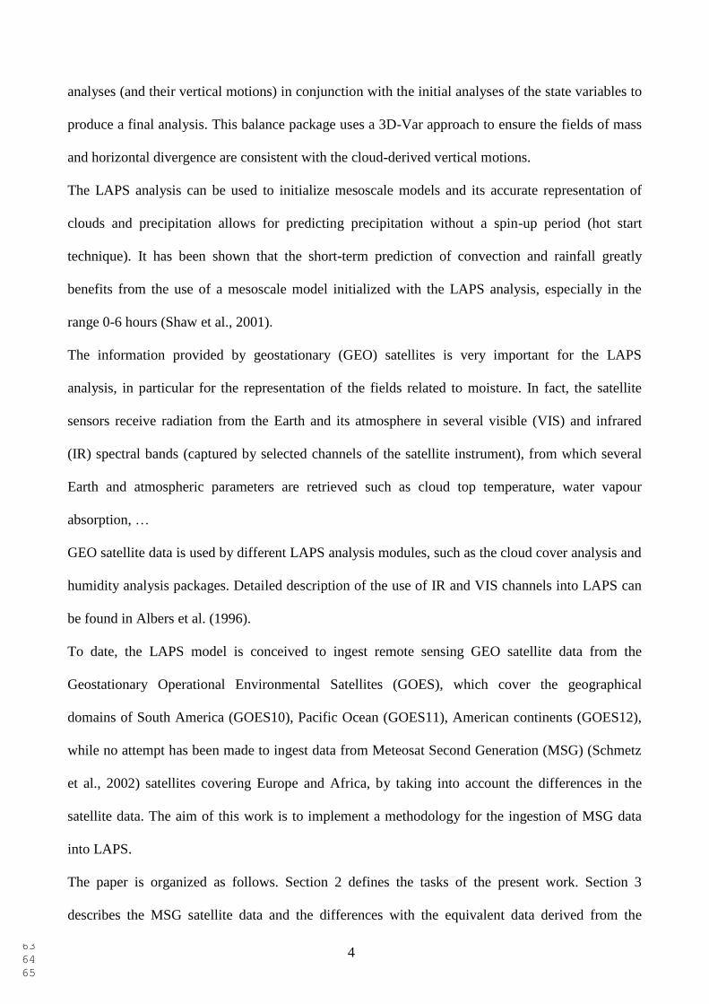
4

analyses (and their vertical motions) in conjunction with the initial analyses of the state variables to

produce a final analysis. This balance package uses a 3D-Var approach to ensure the fields of mass

and horizontal divergence are consistent with the cloud-derived vertical motions.

The LAPS analysis can be used to initialize mesoscale models and its accurate representation of

clouds and precipitation allows for predicting precipitation without a spin-up period (hot start

technique). It has been shown that the short-term prediction of convection and rainfall greatly

benefits from the use of a mesoscale model initialized with the LAPS analysis, especially in the

range 0-6 hours (Shaw et al., 2001).

The information provided by geostationary (GEO) satellites is very important for the LAPS

analysis, in particular for the representation of the fields related to moisture. In fact, the satellite

sensors receive radiation from the Earth and its atmosphere in several visible (VIS) and infrared

(IR) spectral bands (captured by selected channels of the satellite instrument), from which several

Earth and atmospheric parameters are retrieved such as cloud top temperature, water vapour

absorption, …

GEO satellite data is used by different LAPS analysis modules, such as the cloud cover analysis and

humidity analysis packages. Detailed description of the use of IR and VIS channels into LAPS can

be found in Albers et al. (1996).

To date, the LAPS model is conceived to ingest remote sensing GEO satellite data from the

Geostationary Operational Environmental Satellites (GOES), which cover the geographical

domains of South America (GOES10), Pacific Ocean (GOES11), American continents (GOES12),

while no attempt has been made to ingest data from Meteosat Second Generation (MSG) (Schmetz

et al., 2002) satellites covering Europe and Africa, by taking into account the differences in the

satellite data. The aim of this work is to implement a methodology for the ingestion of MSG data

into LAPS.

The paper is organized as follows. Section 2 defines the tasks of the present work. Section 3

describes the MSG satellite data and the differences with the equivalent data derived from the

1 2 3 4 5 6 7 8 9 10 11 12 13 14 15 16 17 18 19 20 21 22 23 24 25 26 27 28 29 30 31 32 33 34 35 36 37 38 39 40 41 42 43 44 45 46 47 48 49 50 51 52 53 54 55 56 57 58 59 60 61 62 63 64 65

5

GOES instruments. Section 4 details the methodologies for the preprocessing of MSG data in order

to obtain a data format suitable for LAPS satellite ingestion phase, based on a Geographic

Information System (GIS) approach and open source components, and the modifications necessary

to the LAPS code to allow for the ingestion of MSG data. Section 5 compares the LAPS cloud

cover analysis with that produced with another analysis tool for MSG data in a case study of a

tropical like cyclone over the Mediterranean Sea. Section 6 concludes the paper discussing the

results and outlines the future developments to improve the methodology.

2. Description of the task

To carry on the ingestion of MSG data into LAPS several kinds of problems have to be faced with:

the modelling of geographic data, the transformation of data into a format suitable for the LAPS

ingestion routine, the identification of the correspondence between radiometric channels of the

GOES instrument and those of the Spinning Enhanced Visible and InfraRed Imager (SEVIRI) on

board MSG, since LAPS reads appropriately only GOES data.

The geographic data model used in this work is a standardized spatial representation of fields

measured over the Earth by the SEVIRI instrument. For our purposes, a raster data model (ISO,

2005) has been chosen since LAPS makes use of this kind of spatial representation. Note that the

raster representation is an abstraction of the real world where spatial data are expressed as a matrix

of cells or pixels where the shape of each cell must be square or rectangular with respect to a

specific coordinate system. The original SEVIRI data are not raster modelled and thus several

operations must be performed on them before they can be ingested into LAPS.

Hereafter the term “geographic data modelling” refers to the extraction of radiometric values from

MSG data, their geographic projection and spatial resample into a spatial grid, which represents the

LAPS simulation domain. These gridded datasets will be stored as 10 bit images (one numerical

1 2 3 4 5 6 7 8 9 10 11 12 13 14 15 16 17 18 19 20 21 22 23 24 25 26 27 28 29 30 31 32 33 34 35 36 37 38 39 40 41 42 43 44 45 46 47 48 49 50 51 52 53 54 55 56 57 58 59 60 61 62 63 64 65

6

matrix for each radiometric channel) in Network Common Data Form (NetCDF) files (Unidata,

2009), that is in the satellite data format used at FSL (Smart and Birkenheuer, 1995) and readable

by LAPS ingest routines. Since the LAPS model ingests radiometric values from 5 channels of the

GOES satellites, each one with specific characteristics in terms of the spectral band and physical

variables that can be extracted from them, the present paper describes also the way the LAPS code

should be modified so that the channels from MSG-SEVIRI corresponding to GOES channels can

be correctly read by the model.

In general, satellite images are produced through a system composed by several instruments,

software and hardware, on board the spacecraft and at the ground stations. Through these

components, images are acquired and successively processed in order to accomplish various kinds

of corrections for radiometric and geometric effects.

For our purposes, this system can be represented as a virtual instrument which reveals radiance

signal incoming from the observed area and for distinct spectral channels. All of these analogic

signals are spatially sampled in order to produce image pixels, and they are also amplified and

transformed into digital numeric values named Digital Numbers (DN) or Digital Counts (DC). Each

one of these instruments may be considered as a black box that we call “radiometric encoder”,

which receives a radiance signal as input and produces a numeric output signal in the form of digital

images.

Such images are completely characterized by their spatial features and by the algorithm relating DN

to radiance values. Thus, to allow the ingestion of MSG into LAPS, it has to be taken into account

that GOES and METEOSAT notably differ in terms of the “radiometric encoder”. Therefore the

LAPS software should be modified in order to accomplish the right conversion from DN to physical

variables like radiance, reflectance or brightness temperature.

3. Data sets

1 2 3 4 5 6 7 8 9 10 11 12 13 14 15 16 17 18 19 20 21 22 23 24 25 26 27 28 29 30 31 32 33 34 35 36 37 38 39 40 41 42 43 44 45 46 47 48 49 50 51 52 53 54 55 56 57 58 59 60 61 62 63 64 65

7

MSG data is described hereafter and a comparison is made between them and GOES data from the

point of view of spectral bands in order to show which SEVIRI channels are good candidates to

replace GOES data into the LAPS model.

The GOES imager is a five-channel instrument designed to measure radiation in the VIS and the IR

portions of the electromagnetic spectrum. LAPS is designed to ingest GOES channel data (a VIS

channel whose spectral band is centred at 0.6μm, a middle-IR channel centred at 3.9 μm, a water

vapour channel centred at 6.7 μm, and two thermal windows channels centred at 11.2 and 12.0 μm,

respectively).

The imager equivalent to the GOES instrument over Europe and Africa is the SEVIRI on board the

MSG-2 satellite (Meteosat9) positioned at 0° longitude and 0° latitude, in geostationary orbit, 35800

km above the Gulf of Guinea. The SEVIRI instrument is made up of 11 spectral channels that

provide measurements with a resolution of 3 km × 3 km at the sub-satellite point every 15 minutes

and a High Resolution Visible (HRV) channel whose measurements have a resolution of 1 km × 1

km.

The SEVIRI data is distributed to the user mainly through the EUMETCast service (EUMETSAT,

2006) or the EUMETSAT Unified Meteorological Archive and Retrieval Facility (UMARF)

(EUMETSAT, 2001). The first is a dissemination system based on standard Digital Video

Broadcast (DVB) technology (EUMETSAT, 2006) that uses commercial telecommunication

geostationary satellites (HotBird at present) to distribute files and allows users to receive images

and data in nearly real time, while the second is a retrieval service based on an on-line access to

data catalogues. Both services provide SEVIRI images processed to Level 1.5 (EUMETSAT,

2007), obtained through the processing of satellite raw data (designated as Level 1.0 data). This

processing level corresponds to image data corrected for radiometric and geometric effects,

geolocated using a standard projection, finally calibrated.

1 2 3 4 5 6 7 8 9 10 11 12 13 14 15 16 17 18 19 20 21 22 23 24 25 26 27 28 29 30 31 32 33 34 35 36 37 38 39 40 41 42 43 44 45 46 47 48 49 50 51 52 53 54 55 56 57 58 59 60 61 62 63 64 65

8

To transform MSG data in a suitable data format for an application it is necessary to know the

format in which the users receive the data via the dissemination service in order to choose the

appropriate software tools to read and process the data.

This data consists of geographical arrays of 3712 × 3712 pixels and a sampling distance of 3 km × 3

km at the sub-satellite point (except the HRV channel), i.e. the point on the Earth’s surface directly

below the satellite. Each pixel contains 10 bit data that represents the radiance value, expressed in

10-3

Wm-2

sr-1

[cm-1

]-1

, codified in DC form.

The full Earth image (for channels 1-11) is composed by 8 segment files, each one consisting of

464 lines. This framework defines the so-called High Rate Image Transmission (HRIT) or Low

Rate Image Transmission (LRIT) segment files (EUMETSAT, 2007). Each file is compressed by

means of a wavelet algorithm.

An inspection of Table 1, which summarizes the spectral characteristics of Meteosat9 SEVIRI

channels, reveals that channels 1,4,5,9 and 10 are the closest to the GOES imager channels in terms

of spectral bands.

However, the procedure of substitution of GOES with MSG channels is not straightforward, since

potentially corresponding channels may considerably differ in terms of spectral response, sensor

calibrations, etc. (Doelling et al., 2004). For example, in terms of spectral response, the radiance

measured in SEVIRI and related GOES channels may significantly differ due to: a) approximate

correspondence among spectral bands, b) different instrument features, and c) calibration and

correction algorithms. Thus a one-to-one substitution of the two imager products into LAPS may

imply large errors in further LAPS processing. Nevertheless, since derived physical variables, as

brightness temperature and albedo, are intrinsic features of the measured object (land, sea and

atmosphere) under specific conditions, they are independent of the instrument. Thus satellite data

substitution is meaningful if the right instructions to render the radiometric MSG values into such

physical variables are provided to LAPS. The method used to solve this issue will be further

explained in the following Sections.

1 2 3 4 5 6 7 8 9 10 11 12 13 14 15 16 17 18 19 20 21 22 23 24 25 26 27 28 29 30 31 32 33 34 35 36 37 38 39 40 41 42 43 44 45 46 47 48 49 50 51 52 53 54 55 56 57 58 59 60 61 62 63 64 65

9

3. The GIS approach

The purpose of the present section is to describe the methods and software tools used to obtain

gridded radiometric values from the five selected SEVIRI channels and to transform them into an

appropriate format for the LAPS satellite ingestion routine.

The grid containing the radiometric values should be consistent with that defined in the LAPS

namelists, concerning geographic and geometric parameters relative to the simulation domain (as

the geographic coordinate system, spatial resolution and geographic extent). As shown in Fig. 1, the

procedure consists of different steps:

Readout of the HRIT image segments containing SEVIRI data.

Geographic re-projection of input data with respect to the LAPS user specified Coordinate

Reference System (CRS) (OGP, 2008).

Spatial re-sample of input data with respect to the LAPS user-specified spatial resolution.

Extraction of geographic window to match the LAPS simulation domain.

Production of input files in a format suitable to be ingested into LAPS.

To accomplish all of these operations, some open-source software tools are chosen. Among the

available open-source projects, the tools that match the functional requirements and that ensure a

good interoperability are selected:

EUMETSAT WaveLet Transform Software (EUMETSAT, 2009c), the tool used to

decompress SEVIRI HRIT data files;

NetCDF (Unidata, 2009), a set of software library data formats that support creation, access,

and sharing of array-oriented scientific data, required as LAPS ingests satellite data file only

in this format;

1 2 3 4 5 6 7 8 9 10 11 12 13 14 15 16 17 18 19 20 21 22 23 24 25 26 27 28 29 30 31 32 33 34 35 36 37 38 39 40 41 42 43 44 45 46 47 48 49 50 51 52 53 54 55 56 57 58 59 60 61 62 63 64 65

10

Geospatial Data Abstraction Library (GDAL, 2009a), an Open Source library which allows

to read and write many geographic data formats, encoding geographical information into

files (GDAL acts as an interface for geospatial operations over the geographic data files for

all supported data formats).

SEVIRI data are delivered in a specific CRS named “GEOS” (CGMS, 1999), i.e. the normalized

geostationary projection that describes the view from a virtual satellite to an idealized Earth. The

distance between the spacecraft and the centre of the Earth is 42164 km. The idealized Earth is a

perfect ellipsoid with an equator radius of 6378 km and a polar radius of 6356 km.

Since the GDAL library (GDAL, 2009b) includes the GEOS projection and it can be compiled

adding the MSG driver support with EUMETSAT’s Wavelet Trasform software, GDAL is an

excellent open source tool to carry out the procedure. As a consequence, SEVIRI HRIT/LRIT

image segment file can be processed as normal raster files. Furthermore GDAL includes NetCDF

among its output file formats.

In conclusion, given a specific MSG acquisition through the GDAL library and for each SEVIRI

channels it is possible to extract a geographic window of data and process them in order to meet

LAPS requirements on satellite input data format. The produced NetCDF files are not yet

conformed to our needs because the LAPS satellite ingestion routine needs NetCDF files, which

have a specific internal structure according to Satellite Broadcast Network (SBN) data model

(NOAA, 1997). Unfortunately, SBN image data contains 8-bits per pixels and thus the adoption of

this data model implies a data loss in terms of radiometric accuracy since SEVIRI data has 10-bits

per pixel. To bypass this issue, the LAPS ingestion routine code has been “hacked” in order to

allow to read modified SBN data model with 10-bits per pixel.

In reality LAPS is able to read satellite data models different from SBN, as gvar, fsl-conus and that

of the AirForce Global Weather Center. Here, SBN has been chosen because it includes more

general satellite data formats that are standard projections so that it is quite independent of the

specific satellite platform.

1 2 3 4 5 6 7 8 9 10 11 12 13 14 15 16 17 18 19 20 21 22 23 24 25 26 27 28 29 30 31 32 33 34 35 36 37 38 39 40 41 42 43 44 45 46 47 48 49 50 51 52 53 54 55 56 57 58 59 60 61 62 63 64 65

11

As an example, Fig. 1 illustrates the GIS process that extracts SEVIRI data from the MSG

acquisition and re-projects them into the LAPS simulation domain. Brighter pixels correspond to

higher radiance values.

Figure 2a is a gray scale SEVIRI image while Fig. 2b shows the re-projected data over a simulation

domain covering Southern Italy.

4. Assimilation procedure of LAPS data ingestion

As anticipated in section 1, LAPS is a complex numerical system conceived to perform gridded

analyses by merging together numerous data sources. Figure 3 summarizes the logical data flow

during the ingestion process. It is organized in four levels: data sources (top box) are formatted for

ingestion routines into LAPS (second box); these routines produce intermediate files (third box)

containing data in a format suitable for the LAPS analysis process (fourth box).

The satellite ingestion process named “lvd_sat_ingest” is now described, which produces satellite

intermediate files with the “lvd” extension starting from MSG data that is in turn pre-processed as

described in the previous section.

The LVD file is generated in NetCDF format. It contains 12 variables derived from the radiometric

values of the 5 satellite channels described in the previous sections. Each variable is composed of a

grid of values that covers the LAPS geographic domain.

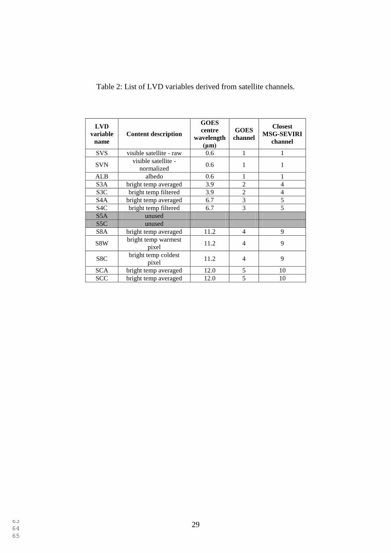
Table 2 shows that two kinds of variables can be distinguished: those derived from the brightness

temperature of the IR channels and those derived from the radiance of the single VIS channel used

in this procedure.

The Lvd_sat_ingest process derives this information from the DCs of the gridded satellite data in

several steps. First of all, it is necessary to convert DC into Radiance (L) and Brightness

Temperature (BT). To accomplish this step, lvd_sat_ingest makes use of the so-called Satellite

1 2 3 4 5 6 7 8 9 10 11 12 13 14 15 16 17 18 19 20 21 22 23 24 25 26 27 28 29 30 31 32 33 34 35 36 37 38 39 40 41 42 43 44 45 46 47 48 49 50 51 52 53 54 55 56 57 58 59 60 61 62 63 64 65

12

Lookup Tables. These tables are automatically generated by the “genlvdlut.exe” LAPS module (on

“localization script”) (NOAA, 2009) and contain the correspondence between DC and L or BT for

each channel and for each satellite acquisition. Since GOES and MSG data are coded differently,

tables suitable for SEVIRI channels have to be created in order to replace the GOES tables.

To determine the radiance for each channel, scaling parameters (cal_slope and cal_offset) have to

be identified. The scaling parameters are contained into the header file named “prologue” of Level

1.5 SEVIRI images. Radiance values can be calculated by means of the following formula

(EUMETSAT, 2008):

L(i,ch) = DC(i,ch) * cal_slope(ch) + cal_offset(ch) (1)

where DC(i,ch) and L(i,ch) are the digital count and radiance of pixel i and channel ch, respectively.

For SEVIRI thermal channels (4-11), brightness temperature, expressed in 10-3

Wm-2

sr-1

[cm-1

]-1

, can

be calculated by simply inverting the Planck function at the channel wavelength, that is:

4

0

10 ,

2

3 1ln1

cBT

c

L

(2)

where λ0 is the central wavelength of the channel expressed in μm and c1 and c2 channel varying

constants listed in the EUMETSAT documents (EUMETSAT, 2007). Figure 4 summarizes the

operational procedure in order to produce the LAPS MSG lookup table.

Finally, some orbital parameters relative to Meteosat9 have to be set into the LAPS routine, namely

the distance between the spacecraft and the centre of the Earth (range_m), and the sub-satellite

geographic coordinates (sublat_d, sublon_d).

After these modifications, the lvd_sat_ingest process can be normally launched to produce lvd

intermediate files from MSG data. Figure 5 shows an example of lvd variables derived from

1 2 3 4 5 6 7 8 9 10 11 12 13 14 15 16 17 18 19 20 21 22 23 24 25 26 27 28 29 30 31 32 33 34 35 36 37 38 39 40 41 42 43 44 45 46 47 48 49 50 51 52 53 54 55 56 57 58 59 60 61 62 63 64 65

13

SEVIRI images (26 September 2006, 1200 UTC). Figure 5a shows the albedo,1 expressed as a

fractional number from 0 to 1 and derived from the VIS channel (0.6 μm), while Fig. 5b shows

averaged BT expressed in K and derived from the IR channel (11 μm) through mean filtering,

which simply means replacing each pixel value in the BT image with the value obtained as average

of the pixel itself with its neighbors.

5. Comparison with the MSG cloud cover products of the SAFNWC

To determine the reliability of the SEVIRI-MSG assimilation into LAPS it is important to ascertain

if LAPS cloud outputs are consistent with the cloud analysis products generated with other tools. As

a first step, some of the LAPS cloud variables are considered and compared with the equivalent

meteorological products derived from the Satellite Application Facility in support to Nowcasting

(SAFNWC). SAFNWC is a project started by EUMETSAT in February 1997 whose general

objective is to ensure the optimal use of meteorological satellite data for nowcasting and very short

range forecasting by means of the development and maintenance of appropriate software packages

(http://nwcsaf.inm.es/).

Cloud cover and cloud top height variables are selected for comparison as they represent important

parameters for nowcasting purposes (they may contribute to the analysis and early warning of

thunderstorm development). Since the SAFNWC software package and LAPS ingest the same MSG

data, the spatial comparison cannot be assumed as a validation process, rather as a pixel by pixel

correspondence verification between these two tools and the consistency of the cloud cover.

1 A rough method has been used to intercalibrate SEVIRI-MSG and GOES11 solar channels (0.6 μm), based on

the assumption (not completely true) that the two detectors reveal the same spectral radiance values. For each pixel, the

solar radiance of SEVIRI instrument has been transformed into digital numeric values (DN), using the same Visible-

channel calibration coefficients as for GOES-11 imagers (http://www.oso.noaa.gov/goes/goes-calibration/goes-vis-ch-

calibration.htm) and then albedo is calculated by mean of LAPS satellite ingestion routine.

1 2 3 4 5 6 7 8 9 10 11 12 13 14 15 16 17 18 19 20 21 22 23 24 25 26 27 28 29 30 31 32 33 34 35 36 37 38 39 40 41 42 43 44 45 46 47 48 49 50 51 52 53 54 55 56 57 58 59 60 61 62 63 64 65

14

A preliminary comparison is performed only for 3 time steps at 0900, 1200 and 1500 UTC on

September 26, 2006 . In the following subsections the characteristics of the region, the SAFNWC

products, the methods employed to make the spatial comparison will be described. A discussion of

the results will be followed by a meteorological analysis that checks the ability of the LAPS

analysis in reproducing the correct meteorological features of the case study.

5.1. Geographic area characteristics

The geographic domain under consideration is approximately centred over Southern Italy. It spreads

from 37.86 to 43.15 °N and from 14.03 to 20.96 °E, covers an area of 596 × 516 km2 and is

characterized by a complex topography alternate to lowland and sea.

South-eastern Italy is the area affected by the tropical-like cyclone that will be analyzed hereafter

(Moscatello et al., 2008a). This region is surrounded by the Ionian and Adriatic seas and thus the

role of latent and sensible heat fluxes between the sea surface and the atmosphere can be very

important in intensifying storms and cyclones, especially in late summer and early fall when the sea

surface is still relatively warm.

5.2. SAFNWC meteorological products

Cloud cover LAPS analysis has been compared with the cloud cover produced by the SAFNWC

software. In particular, the meteorological SAF product named Cloud Top Temperature and Height

(CTTH) (EUMETSAT, 2009a) is considered. CTTH constitutes a class of MSG cloud products,

computed through a processing sequence of Cloud Mask, Cloud Type and Cloud Top Height. This

processing sequence makes use of several input data, which includes almost all MSG SEVIRI

channel data and numerical weather prediction (NWP) parameters. NWP data used in this work are

1 2 3 4 5 6 7 8 9 10 11 12 13 14 15 16 17 18 19 20 21 22 23 24 25 26 27 28 29 30 31 32 33 34 35 36 37 38 39 40 41 42 43 44 45 46 47 48 49 50 51 52 53 54 55 56 57 58 59 60 61 62 63 64 65

15

provided by the European Centre for Medium-Range Weather Forecasts (ECMWF,

http://www.ecmwf.int/) in GRIdded Binary (GRIB) format.

The SAFNWC software produces its output at SEVIRI IR full spatial resolution over any

rectangular areas defined by the user inside the MSG full disk. Within the chosen geographic

window, the SEVIRI IR spatial resolution ranges approximately from 4 to 5 Km.

Cloud Top Height data is produced as a 7 bit numerical matrix stored in Hierarchical Data Format

(HDF) files. In order to extract the height (in m) of the cloud top, a linear conversion from count to

height is needed through the following formula:

Cloud Height = gain * Count7bits + intercept (3)

where gain and intercept are equal, respectively, to 200 m count-1

and -2000 m (EUMETSAT,

2009b).

5.3. Methods

To provide a consistent comparison, SAFNWC products are first mapped onto the LAPS’s

geographic projection, grid domain, and horizontal resolution. The projection chosen for the LAPS

analysis is the Lambert Conformal Conic with a horizontal resolution of 4 km, which is close to the

original resolution of SEVIRI IR data relative to our geographic window.

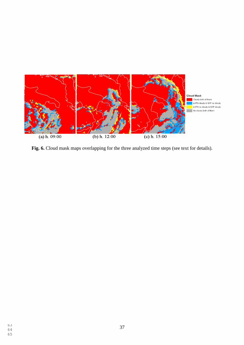
The comparison process between LAPS and SAFNWC cloud products occurs in two main steps.

First, for each time step taken into account, LAPS and SAFNWC cloud masks are geographically

overlapped to generate a spatial pattern that allows to identify the differences in cloud cover

outputs. Figure 6 shows the areas where clouds are identified by one, both or neither of the two

tools. To obtain a more quantitative comparison, these results are summarized in contingency tables

as shown in Table 3. Two indices are used to quantify the differences between the two analyses, the

1 2 3 4 5 6 7 8 9 10 11 12 13 14 15 16 17 18 19 20 21 22 23 24 25 26 27 28 29 30 31 32 33 34 35 36 37 38 39 40 41 42 43 44 45 46 47 48 49 50 51 52 53 54 55 56 57 58 59 60 61 62 63 64 65

16

BIAS and PC (Proportion Correct or Hit rate) (Hyvärinen, 2007), which are calculated from the

contingency table and expressed as

BIAS = (A+B)/(A+C) (4)

and PC=(A+D)/(A+B+C+D) (5)

When BIAS = 1 there is an equal amount of cloudy pixels in both analysis (although it does not

imply a perfect spatial overlap). When the BIAS smaller (larger) than 1, there are less (more)

cloudy pixels in the LAPS outputs with respect to the SAFNWC outputs. The PC index is more

informative on the mutual spatial location of cloudy pixels. When PC = 1 there is a total agreement

between the analyses while, conversely, when PC = 0 there is a total disagreement.

Second, the differences between LAPS and SAFNWC cloud top heights are derived. As in the

cloud mask comparison, cloud top height maps are overlapped and a height difference is generated

pixel by pixel. Note that height differences are computed only on the pixels which come out cloudy

in both analyses, as shown in Fig. 6.

Finally, the LAPS and SAFNWC cloud top heights are compared using a simple linear regression

as a more rigorous consistency test. Scatterplots and coefficients of determination r2 (Hiemstra et

al., 2006) are also calculated to show how LAPS cloud top height are distributed with respect to

SAFNWC data and to quantify how well the linear regression approximates the relationship

between the two analysis.

Since there is not a straightforward way to establish appropriate thresholds that separate outliers

from the correct pixels, sub-distributions of pixel by pixel absolute differences between the two

cloud heights are computed. They include only the subsets (70%, 80% or 90%) of pixels that show

the smallest discrepancies. Then linear regressions, scatter plots and r2 are computed on such

subsets. The use of three different pixel subsets, allows to better identify the degradation trend of

1 2 3 4 5 6 7 8 9 10 11 12 13 14 15 16 17 18 19 20 21 22 23 24 25 26 27 28 29 30 31 32 33 34 35 36 37 38 39 40 41 42 43 44 45 46 47 48 49 50 51 52 53 54 55 56 57 58 59 60 61 62 63 64 65

17

the statistical parameters (i.e., r2) when a larger number of pixels are considered. Thus more

complete information is provided about the matching between SAFNWC and LAPS cloud cover.

5.4. Results

In Table 4 the results of the cloud mask comparison are shown for the three analyzed time steps.

BIAS and PC values are close to 1 demonstrating a generally good agreement between LAPS and

SAFNWC for both amount and spatial location of cloudy pixels, as shown in Fig. 6.

The third time step (1500 UTC) shows the worst result since LAPS reveals a larger amount of

cloudy pixels localized in the lower right corner of the domain (Fig. 6c). A more thorough analysis

reveals that LAPS produces a different response with respect to SAFNWC especially in the areas

where clouds are thin and sparse (Fig. 7a). In fact, Fig. 7b shows that in the lower right corner

LAPS detects a cloud cover less than 30%.

Note that cloud cover provided with the METeorological Aerodrome Reports (METAR), even

though representing a rough set of information, is a very important first guess for the LAPS cloud

detection in the lower troposphere (Albers et al., 1996). Absence of METAR cloud cover

information prevents the LAPS analysis from accurately producing clouds below 5 km altitude. As

an example, Fig. 8 shows the effect of removing METAR information from the LAPS analysis at

0900 UTC. By comparing Fig. 6a, that has been obtained by including just one METAR inland

Calabria region, and Fig.8b it is possible to observe the absence of cloud cover over the south-

western area in the LAPS analysis, while in the MSG image low and medium cloud tops are

present.

Figure 9 and 10 show the cloud top height and their difference maps, respectively, expressed as

absolute values (derived from the analysis with LAPS and SAFNWC) for the three time steps. From

this preliminary analysis it is possible to see that in most of the domain the difference in cloud top

1 2 3 4 5 6 7 8 9 10 11 12 13 14 15 16 17 18 19 20 21 22 23 24 25 26 27 28 29 30 31 32 33 34 35 36 37 38 39 40 41 42 43 44 45 46 47 48 49 50 51 52 53 54 55 56 57 58 59 60 61 62 63 64 65

18

height is smaller than 1 km. Generally, such differences are smaller in the areas where there is a

more uniform cloud cover.

Some differences can be attributed, at least partially, to a slight offset in the location of cloudy

pixels. Although map reprojections have been accurately crafted, we suppose that SAFNWC and

LAPS pixels refer to slightly different areas and this fact, combined with the fine spatial resolution

(4 km), can lead to errors in some pixels, especially in the areas where the cloud cover or height is

not uniform.

Figure 11 illustrates some statistical relationships between cloud top heights computed with

SAFNWC and LAPS. Rows indicate the time step, while columns show the percentage of cloudy

pixels taken into account as described in subsection 5.3.

The scatterplots make it easy to note that the data points are distributed mainly along the green

regression line. A large number of dot clusters on the right side of the panels, especially for

the percentile q = 90%, and this means that LAPS generally underestimates the cloud top height

with respect to SAFNWC. This underestimation of LAPS is probably due to the fact that LAPS is

fit for GOES channels and not for MSG, that implies an imperfect calibration for the SEVIRI 11 μm

channel spectral width. In fact, the BTs derived from this channel are fundamental for the definition

of cloud top height. It may also be that LAPS is assigning too great an optical depth to these clouds

(Albers et al., 1996).

The fact that the coefficients of determination range from 0.56 to 0.93 means that the linear model

constitutes an acceptable approximation in describing the relationship between the two analyses.

The high r2 values for all the different percentile thresholds indicate that most of the pixels of the

LAPS analysis generally fit well with SAFNWC analysis.

In conclusion, the case study shows that the ingestion of MSG-SEVIRI data into LAPS works quite

well in reproducing the cloud horizontal structure, at least in the analyzed case study. More

informed conclusions would require a long time series of analysis to develop a statistically

meaningful evaluation.

1 2 3 4 5 6 7 8 9 10 11 12 13 14 15 16 17 18 19 20 21 22 23 24 25 26 27 28 29 30 31 32 33 34 35 36 37 38 39 40 41 42 43 44 45 46 47 48 49 50 51 52 53 54 55 56 57 58 59 60 61 62 63 64 65

19

d) Meteorological analysis

In order to verify the ability of the LAPS analysis in reproducing the characteristics of the cyclone

that affected south-eastern Italy on 26 September 2006, mean sea level pressure (MSLP) and a

vertical cross section of wind, temperature and humidity have also been examined.

Although the MSLP fields computed by LAPS surface processing is based on several input data

(McGinley et al., 1991), our study revealed that background data represents the most important

source of information.

Two types of background are used to initialize LAPS: the ECMWF data and the Weather Research

and Forecasting (WRF) model (Skamarock et al., 1999) forecasts shown in Moscatello et al.

(2008b). It is noted that the use of different background data has no significant influence on the

cloud top height and cloud cover, whereas it determines a strong impact on the MSLP field. Figures

12 and 13 show the LAPS analysis MSLP for 3 time steps using WRF forecast and ECMWF data,

respectively. The two background fields produce fairly different MSLP analyses. In particular, we

see that the cyclone generated with the WRF model forecast as background fields reproduces the

structure generated in Moscatello et al. (2008b).

Figure 14 shows the wind speed and the potential temperature in a vertical cross section at the

latitude of the pressure minimum (that is located approximately in the middle of the figure), at 12

UTC, 26 September, when the cyclone has completely developed the characteristics typical of

tropical cyclones. Similarly as in Moscatello et al. (2008b)'s Fig. 17, we see a minimum wind speed,

of 6 m s-1

, in correspondence with the centre of the cyclone; also, a maximum of 26 m s-1

is

located about 30 km far from the centre, on the eastern side of the low. Above the centre, the

existence of a warm core is apparent in the layer between 850 and 650 hPa. Thus, the vertical

structure emerging from the LAPS analysis is consistent with that expected for a tropical-like

cyclone.

1 2 3 4 5 6 7 8 9 10 11 12 13 14 15 16 17 18 19 20 21 22 23 24 25 26 27 28 29 30 31 32 33 34 35 36 37 38 39 40 41 42 43 44 45 46 47 48 49 50 51 52 53 54 55 56 57 58 59 60 61 62 63 64 65

20

Conclusion and future work

Software for the ingestion of MSG SEVIRI satellite data in the VIS and IR spectral bands into the

Local Analysis and Prediction System (LAPS) is written and tested. Note that LAPS is originally

designed for the input of GOES satellite data and its use outside the Conterminous United States

(CONUS) area often has limitations. The present work represents a first step towards an operational

use of LAPS over Europe using EUMETSAT’s GEO satellites.

The sensitivity of the LAPS scheme to the ingestion of VIS and IR data from Meteosat is examined

by comparing its cloud analyses with those of EUMETSAT’s Nowcasting SAF. Results are very

encouraging, though a general underestimation of cloud top height is found for LAPS with respect

to SAFNWC. This suggests that adjustments are needed to transform the original GOES-based

LAPS cloud scheme into the new MSG-based presented in the paper. This will be the first step to be

done towards the improvement of the current version of the software.

The above mentioned comparison has also shown that the initialisation of the LAPS analysis with

different background fields such as those of ECMWF and WRF has scarce influence on the derived

cloud parameters while producing significantly different MSLP maps. Further studies are needed in

this area to better understand these results, which depend, among the other factors, on the resolution

of the input background fields.

Note that the present study is a first important step towards using physical analyses for mesoscale

NWP models initialisation over Europe. Moreover, the LAPS scheme based on Meteosat is

expected to be very instrumental for weather monitoring, particularly in case of complex and

intense events. In this direction its use for meteorology, civil protection, hazard management and

generally for nowcasting and very short range forecasting is to be considered in a short while.

1 2 3 4 5 6 7 8 9 10 11 12 13 14 15 16 17 18 19 20 21 22 23 24 25 26 27 28 29 30 31 32 33 34 35 36 37 38 39 40 41 42 43 44 45 46 47 48 49 50 51 52 53 54 55 56 57 58 59 60 61 62 63 64 65

21

Acknowledgments

The authors are grateful to Regione Puglia for support provided under the Progetto Strategico

“Nowcasting avanzato con l’uso di tecnologie GRIS e GIS”. VL also wishes to acknowledge partial

support from the Italian Space Agency (ASI) within the project “Prodotti di Osservazione

Satellitare per Allerta Meteorologica” (PROSA) and from EUMETSAT within the Satellite

Application Facility on Support to Operational Hydrology and Water Management (H-SAF).

Thanks also to Spanish State Meteorological Agency (AEMET) for SAFNWC/PPS and

SAFNWC/MSG software provided by AEMET on behalf of EUMETSAT and the Nowcasting

SAF Consortium.

1 2 3 4 5 6 7 8 9 10 11 12 13 14 15 16 17 18 19 20 21 22 23 24 25 26 27 28 29 30 31 32 33 34 35 36 37 38 39 40 41 42 43 44 45 46 47 48 49 50 51 52 53 54 55 56 57 58 59 60 61 62 63 64 65

22

References

Albers, S., 1995. The LAPS wind analysis. Wea. Forecasting 10, 342-352.

Albers, S., McGinley, J., Birkenheuer, D., Smart, J., 1996. The Local Analysis and Prediction System (LAPS): Analyses of clouds,

precipitation, and temperature. Wea. Forecasting 11, 273-287.

Birkenheuer, D., 1999. The effect of using digital satellite imagery in the LAPS moisture analysis. Wea. Forecasting 14, 782-788.

CGMS, 1999. LRIT/HRIT global specification. [available from

http://www.eumetsat.int/groups/cps/documents/document/pdf_cgms_03.pdf]

Doelling, D. R., Minnis, P., Nguyen, L., 2004. Calibration comparisons between SEVIRI, MODIS, and GOES data. [available from

http://www-pm.larc.nasa.gov/msg/pub/conference/Doelling.MSG.RAO.04.pdf]

EUMETSAT, 2001. The Meteosat archive - User handbook, Technical Description 06. [available from

http://www.eumetsat.int/idcplg?IdcService=GET_FILE&dDocName=pdf_td06_marf&RevisionSelectionMethod=LatestReleased

]

EUMETSAT, 2006. EUMETCast - EUMETSAT's broadcast system for environmental data, Technical Description 15. [available

from

http://www.eumetsat.int/idcplg?IdcService=GET_FILE&dDocName=pdf_td15_eumetcast&RevisionSelectionMethod=LatestRel

eased]

EUMETSAT, 2007a. A planned change to the MSG Level 1.5 image product radiance definition, document n. 0519. Available from:

http://www.eumetsat.int/idcplg?IdcService=GET_FILE&dDocName=PDF_MSG_PLANNED_CHANGE_LEVEL15&Revision

SelectionMethod=LatestReleased.

EUMETSAT, 2007b. MSG Level 1.5 image data format description, Format Guide v5a. [available from:

http://www.eumetsat.int/idcplg?IdcService=GET_FILE&dDocName=pdf_ten_05105_msg_img_data&RevisionSelectionMethod

=LatestReleased]

EUMETSAT, 2008. A simple conversion from effective radiance back to spectral radiance for MSG images, document n. 1053.

[available from:

http://www.eumetsat.int/idcplg?IdcService=GET_FILE&dDocName=pdf_msg_conv_effrad2specrad&RevisionSelectionMethod

=LatestReleased]

EUMETSAT, 2009a. Algorithm theoretical basis document for “Cloud Products”, NWC SAF, CMa-PGE01 v2.0, CT-PGE02 v1.5 &

CTTH-PGE03 v2.0. [available from http://nwcsaf.org/Scientific%20documentation/SAFNWC-CDOP-MFL-SCI-ATBD-

01_v2.0.pdf]

EUMETSAT, 2009b. Product user manual for “Cloud Products”, NWC SAF, CMa-PGE01 v2.0, CT-PGE02 v1.5 & CTTH-PGE03

v2.0 [available from http://nwcsaf.org/Scientific%20documentation/SAFNWC-CDOP-MFL-SCI-PUM-01_v2.0.pdf]

1 2 3 4 5 6 7 8 9 10 11 12 13 14 15 16 17 18 19 20 21 22 23 24 25 26 27 28 29 30 31 32 33 34 35 36 37 38 39 40 41 42 43 44 45 46 47 48 49 50 51 52 53 54 55 56 57 58 59 60 61 62 63 64 65

23

EUMETSAT, 2009c. WaveLet Transform Software. [available from

http://www.eumetsat.int/Home/Main/Access_to_Data/User_Support/SP_1117714787347#wavelet]

GDAL, 2009a. Geospatial Data Abstraction Library (GDAL) v. 1.6. [available from http://www.gdal.org]

GDAL, 2009b. GDAL release news. [available from http://trac.osgeo.org/gdal/wiki/Release/1.6.0-News]

Hiemstra, C. A., Liston, G. E., Pielke, R. A. Sr., Birkenheur, D. L., Albers, S. C., 2006. Comparing Local Analysis and Prediction

System (LAPS) assimilations with independent observations. Wea. Forecasting 21, 1024-1040.

Hyvärinen, O., 2007. Intercomparison of satellite products and in-situ analysis for snow. Joint EUMETSAT Meteorological Satellite

Conf. and 15th AMS Satellite Meteorology & Oceanography Conf., Amsterdam, 24-28 Sept.

ISO, 2005. ISO/TC211 Technical Committee, 2005. Standard n. 19125: Geographic information - Schema for coverage geometry

and functions. [available from http://www.iso.org/iso/iso_catalogue/catalogue_tc/catalogue_detail.htm?csnumber=40121]

McGinley, J. A., Smart, J. R., 2001. On providing a cloud-balanced initial condition for diabatic initialization. Prepr. 18th AMS Conf.

on Weather Analysis and Forecasting, Ft. Lauderdale, FL.

McGinley, J. A., Albers, S. C., Stamus, P. A., 1991. Validation of a composite convective index as defined by a real-time local

analysis system. Wea. Forecasting 6, 337–356.

McGinley, J. A., Albers, S. C., Stamus, P. A., 1992. Local data assimilation and analysis for nowcasting. Adv. Space Res. 12, 179-

188.

McGinley, J. A., Birkenheuer, D., Shaw, B., Schultz, P., 2000. The LAPS water in all phases analysis: The approach and impacts on

numerical prediction. Proc. 5th AMS Int. Symp. on Tropospheric Profiling, Adelaide, 133-135.

Moscatello, A., M. M. Miglietta, R. Rotunno, 2008a, Observational analysis of a Mediterranean “hurricane” over south-eastern Italy,

Weather, 63, 306-311

Moscatello, A., Miglietta, M. M., Rotunno, R., 2008b. Numerical analysis of a Mediterranean “hurricane” over Southeastern Italy.

Mon. Wea. Rev. 136, 4373–4397.

NOAA, 1997. AWIPS-GOES Data Utilization Page. [available from http://laps.noaa.gov/birk/awipsgoes/goesinfo.html]

NOAA, 2009. LAPS README file. [available from http://laps.noaa.gov/software/README.html]

OGP, 2008. Surveying and positioning guidance Note I - Geodetic awareness guidance note, International Association of Oil & Gas

Producers (OGP). [available from http://www.ogp.org.uk/pubs/373-01.pdf]

Schmetz, J., Pili, P., Tjemkes, S., Just, D., Kerkmann, J., Rota, S., Ratier, A., 2002. An introduction to Meteosat Second Generation

(MSG). Bull. Amer. Meteor. Soc. 83, 977-992.

Schultz, P., Albers, S., 2001. The use of three-dimensional analyses of cloud attributes for diabatic initialization of mesoscale

models. Prepr. 14th AMS Conf. on Numerical Weather Prediction, Ft. Lauderdale, FL.

1 2 3 4 5 6 7 8 9 10 11 12 13 14 15 16 17 18 19 20 21 22 23 24 25 26 27 28 29 30 31 32 33 34 35 36 37 38 39 40 41 42 43 44 45 46 47 48 49 50 51 52 53 54 55 56 57 58 59 60 61 62 63 64 65

24

Shaw, B. L., Thaler, E., Szoke, E., 2001. Operational evaluation of the LAPS−MM5 "hot start" local forecast model. Proc. 18th AMS

Conf. on Weather Analysis and Forecasting, Fort Lauderdale, FL, J2.6.

Skamarock, W. C., Rotunno, R., Klemp, J. B., 1999. Models of coastally trapped disturbances. J. Atmos. Sci. 56, 3349–3365.

Smart, J. R., Birkenheuer, D., 1995. Quantitative use of satellite image data formatted for AWIPS. [available from

http://laps.fsl.noaa.gov/birk/dallas95.ps]

Unidata, 2009. Network Common Data Form. [available from http://www.unidata.ucar.edu/software/netcdf/]

1 2 3 4 5 6 7 8 9 10 11 12 13 14 15 16 17 18 19 20 21 22 23 24 25 26 27 28 29 30 31 32 33 34 35 36 37 38 39 40 41 42 43 44 45 46 47 48 49 50 51 52 53 54 55 56 57 58 59 60 61 62 63 64 65

25

Figure captions

Fig.1. Data flow of SEVIRI data pre-processing.

Fig. 2. SEVIRI sub-image extraction for the LAPS geographic domain used in the paper. (a)

Channel 1 (VIS 0.6 μm) image relative to 10 July 2008 at 1400 UTC. Geometric and geographic

features of the LAPS grid used as test case are: grid spacing 4 km, grid dimensions (nx × ny) 129 ×

149, projection system Lambert Conformal Conic, corner points (lat, lon) SW = (37.86, 14.03), SE

= (37.26, 19.79), NW = (43.15, 14.76) and NE = (42.50, 20.96).

Fig. 3. The LAPS ingestion scheme.

Fig. 4. Data flow of lookup tables creation.

Fig. 5. Visible albedo and averaged brightness temperature (11 μm) contained into the LVD file at

1200 UTC.

Fig. 6. Cloud mask maps overlapping for the three analyzed time steps (see text for details).

Fig. 7. (a) Meteosat RGB composite channels 3,2,1; (b) LAPS cloudiness map at 1500 UTC.

Fig. 8. (a) Meteosat RGB composite channels 3,2,1; (b) LAPS cloud mask at 0900 UTC obtained

without METAR data.

Fig. 9. Cloud top heights (m) derived from LAPS and SAFNWC at the three time steps of Fig. 6.

1 2 3 4 5 6 7 8 9 10 11 12 13 14 15 16 17 18 19 20 21 22 23 24 25 26 27 28 29 30 31 32 33 34 35 36 37 38 39 40 41 42 43 44 45 46 47 48 49 50 51 52 53 54 55 56 57 58 59 60 61 62 63 64 65

26

Fig. 10. Absolute values of cloud top height differences for the three time steps of Fig. 6.

Fig. 11. Scatter plot and linear regression with relative coefficient of determination (r2), using

subset indicated by percentiles (q), for the three time steps of Fig. 6.

Fig. 12. MSLP for three time steps using WRF forecast as LAPS background.

Fig. 13. MSLP for three time steps using ECMWF data as LAPS background.

Fig. 14. Vertical cross section along 42°N of the wind velocity (m s-1

,black lines) and potential

temperature (K, colour-shaded area), traversing the pressure minimum axis (16.6°E) at 12:00 UTC,

26 Sep. The horizontal axis represents the longitude expressed in decimal degrees, while vertical

axis represents the pressure vertical levels expressed in hPa.

1 2 3 4 5 6 7 8 9 10 11 12 13 14 15 16 17 18 19 20 21 22 23 24 25 26 27 28 29 30 31 32 33 34 35 36 37 38 39 40 41 42 43 44 45 46 47 48 49 50 51 52 53 54 55 56 57 58 59 60 61 62 63 64 65

27

Table captions

Table 1: MSG SEVIRI Spectral channel definition (EUMETSAT Format Guide v5a).

Table 2: List of LVD variables derived from satellite channels.

Table 3: Contingency table prototype.

Table 4: Spatial comparison index of cloud cover.

1 2 3 4 5 6 7 8 9 10 11 12 13 14 15 16 17 18 19 20 21 22 23 24 25 26 27 28 29 30 31 32 33 34 35 36 37 38 39 40 41 42 43 44 45 46 47 48 49 50 51 52 53 54 55 56 57 58 59 60 61 62 63 64 65

28

Table 1: MSG SEVIRI Spectral channel definition (EUMETSAT Format Guide v5a).

Channel

Number

Channel

Name

Bands Centre

wavelength

(μm)

Spectral Band

(99% energy limits)

(μm)

1 VIS0.6 Visible 0.635 0.56 - 0.71

2 VIS0.8 Visible 0.81 0.74 - 0.88

3 IR1.6 Near-infrared 1.64 1.50 - 1.78

4 IR3.9 Window 3.92 3.48 - 4.36

5 WV6.2 Water-vapour 6.25 5.35 - 7.15

6 WV7.3 Water-vapour 7.35 6.85 - 7.85

7 IR8.7 Window 8.70 8.30 - 9.10

8 IR9.7 Ozone 9.66 9.38 - 9.94

9 IR10.8 Window 10.80 9.80 - 11.80

10 IR12.0 Window 12.00 11.00 - 13.00

11 IR13.4 Carbon dioxide 13.40 12.40 - 14.40

12 HRV Visible (Broad

band)

0.75 0.6 - 0.9

1 2 3 4 5 6 7 8 9 10 11 12 13 14 15 16 17 18 19 20 21 22 23 24 25 26 27 28 29 30 31 32 33 34 35 36 37 38 39 40 41 42 43 44 45 46 47 48 49 50 51 52 53 54 55 56 57 58 59 60 61 62 63 64 65

29

Table 2: List of LVD variables derived from satellite channels.

LVD

variable

name

Content description

GOES

centre

wavelength

(μm)

GOES

channel

Closest

MSG-SEVIRI

channel

SVS visible satellite - raw 0.6 1 1

SVN visible satellite -

normalized 0.6 1 1

ALB albedo 0.6 1 1

S3A bright temp averaged 3.9 2 4

S3C bright temp filtered 3.9 2 4

S4A bright temp averaged 6.7 3 5

S4C bright temp filtered 6.7 3 5

S5A unused

S5C unused

S8A bright temp averaged 11.2 4 9

S8W bright temp warmest

pixel 11.2 4 9

S8C bright temp coldest

pixel 11.2 4 9

SCA bright temp averaged 12.0 5 10

SCC bright temp averaged 12.0 5 10

1 2 3 4 5 6 7 8 9 10 11 12 13 14 15 16 17 18 19 20 21 22 23 24 25 26 27 28 29 30 31 32 33 34 35 36 37 38 39 40 41 42 43 44 45 46 47 48 49 50 51 52 53 54 55 56 57 58 59 60 61 62 63 64 65

30

Table 3: Contingency table prototype.

Cloudy pixels for LAPS/SAFNWC SAFNWC cloudy SAFNWC no cloudy

Laps cloudy A B

Laps no cloudy C D

1 2 3 4 5 6 7 8 9 10 11 12 13 14 15 16 17 18 19 20 21 22 23 24 25 26 27 28 29 30 31 32 33 34 35 36 37 38 39 40 41 42 43 44 45 46 47 48 49 50 51 52 53 54 55 56 57 58 59 60 61 62 63 64 65

31

Table 4: Spatial comparison index of cloud cover.

Time step/indexes BIAS PC

0900 1.059571 0.896936

1200 1.016894 0.915925

1500 1.147280 0.823943

1 2 3 4 5 6 7 8 9 10 11 12 13 14 15 16 17 18 19 20 21 22 23 24 25 26 27 28 29 30 31 32 33 34 35 36 37 38 39 40 41 42 43 44 45 46 47 48 49 50 51 52 53 54 55 56 57 58 59 60 61 62 63 64 65

32

Fig.1. Data flow of SEVIRI data pre-processing.

1 2 3 4 5 6 7 8 9 10 11 12 13 14 15 16 17 18 19 20 21 22 23 24 25 26 27 28 29 30 31 32 33 34 35 36 37 38 39 40 41 42 43 44 45 46 47 48 49 50 51 52 53 54 55 56 57 58 59 60 61 62 63 64 65

33

Fig. 2. SEVIRI sub-image extraction for the LAPS geographic domain used in the paper. (a)

Channel 1 (VIS 0.6 μm) image relative to 10 July 2008 at 1400 UTC. Geometric and geographic

features of the LAPS grid used as test case are: grid spacing 4 km, grid dimensions (nx × ny) 129 ×

149, projection system Lambert Conformal Conic, corner points (lat, lon) SW = (37.86, 14.03), SE

= (37.26, 19.79), NW = (43.15, 14.76) and NE = (42.50, 20.96).

1 2 3 4 5 6 7 8 9 10 11 12 13 14 15 16 17 18 19 20 21 22 23 24 25 26 27 28 29 30 31 32 33 34 35 36 37 38 39 40 41 42 43 44 45 46 47 48 49 50 51 52 53 54 55 56 57 58 59 60 61 62 63 64 65

34

Fig. 3. The LAPS ingestion scheme.

1 2 3 4 5 6 7 8 9 10 11 12 13 14 15 16 17 18 19 20 21 22 23 24 25 26 27 28 29 30 31 32 33 34 35 36 37 38 39 40 41 42 43 44 45 46 47 48 49 50 51 52 53 54 55 56 57 58 59 60 61 62 63 64 65

35

Fig. 4. Data flow of lookup tables creation.

1 2 3 4 5 6 7 8 9 10 11 12 13 14 15 16 17 18 19 20 21 22 23 24 25 26 27 28 29 30 31 32 33 34 35 36 37 38 39 40 41 42 43 44 45 46 47 48 49 50 51 52 53 54 55 56 57 58 59 60 61 62 63 64 65

36

Fig. 5. Visible albedo and averaged brightness temperature (11 μm) contained into the LVD file at

1200 UTC.

1 2 3 4 5 6 7 8 9 10 11 12 13 14 15 16 17 18 19 20 21 22 23 24 25 26 27 28 29 30 31 32 33 34 35 36 37 38 39 40 41 42 43 44 45 46 47 48 49 50 51 52 53 54 55 56 57 58 59 60 61 62 63 64 65

37

Fig. 6. Cloud mask maps overlapping for the three analyzed time steps (see text for details).

1 2 3 4 5 6 7 8 9 10 11 12 13 14 15 16 17 18 19 20 21 22 23 24 25 26 27 28 29 30 31 32 33 34 35 36 37 38 39 40 41 42 43 44 45 46 47 48 49 50 51 52 53 54 55 56 57 58 59 60 61 62 63 64 65

38

Fig. 7. (a) Meteosat RGB composite channels 3,2,1; (b) LAPS cloudiness map at 1500 UTC.

1 2 3 4 5 6 7 8 9 10 11 12 13 14 15 16 17 18 19 20 21 22 23 24 25 26 27 28 29 30 31 32 33 34 35 36 37 38 39 40 41 42 43 44 45 46 47 48 49 50 51 52 53 54 55 56 57 58 59 60 61 62 63 64 65

39

Fig. 8. (a) Meteosat RGB composite channels 3,2,1; (b) LAPS cloud mask at 0900 UTC obtained

without METAR data.

1 2 3 4 5 6 7 8 9 10 11 12 13 14 15 16 17 18 19 20 21 22 23 24 25 26 27 28 29 30 31 32 33 34 35 36 37 38 39 40 41 42 43 44 45 46 47 48 49 50 51 52 53 54 55 56 57 58 59 60 61 62 63 64 65

40

Fig. 9. Cloud top heights (m) derived from LAPS and SAFNWC at the three time steps of Fig. 6.

1 2 3 4 5 6 7 8 9 10 11 12 13 14 15 16 17 18 19 20 21 22 23 24 25 26 27 28 29 30 31 32 33 34 35 36 37 38 39 40 41 42 43 44 45 46 47 48 49 50 51 52 53 54 55 56 57 58 59 60 61 62 63 64 65

41

Fig. 10. Absolute values of cloud top height differences for the three time steps of Fig. 6.

1 2 3 4 5 6 7 8 9 10 11 12 13 14 15 16 17 18 19 20 21 22 23 24 25 26 27 28 29 30 31 32 33 34 35 36 37 38 39 40 41 42 43 44 45 46 47 48 49 50 51 52 53 54 55 56 57 58 59 60 61 62 63 64 65

42

Fig. 11. Scatter plot and linear regression with relative coefficient of determination (r2), using

subset indicated by percentiles (q), for the three time steps of Fig. 6.

1 2 3 4 5 6 7 8 9 10 11 12 13 14 15 16 17 18 19 20 21 22 23 24 25 26 27 28 29 30 31 32 33 34 35 36 37 38 39 40 41 42 43 44 45 46 47 48 49 50 51 52 53 54 55 56 57 58 59 60 61 62 63 64 65

43

Fig. 12. MSLP for three time steps using WRF forecast as LAPS background,

1 2 3 4 5 6 7 8 9 10 11 12 13 14 15 16 17 18 19 20 21 22 23 24 25 26 27 28 29 30 31 32 33 34 35 36 37 38 39 40 41 42 43 44 45 46 47 48 49 50 51 52 53 54 55 56 57 58 59 60 61 62 63 64 65

44

Fig. 13. MSLP for three time steps using ECMWF data as LAPS background

1 2 3 4 5 6 7 8 9 10 11 12 13 14 15 16 17 18 19 20 21 22 23 24 25 26 27 28 29 30 31 32 33 34 35 36 37 38 39 40 41 42 43 44 45 46 47 48 49 50 51 52 53 54 55 56 57 58 59 60 61 62 63 64 65

45

Fig. 14. Vertical cross section along 42N of the wind velocity (ms-1,black lines) and potential

temperature (K, colour-shaded area), traversing the pressure minimum axis (16.6E) at 12:00 UTC

26 Sep. The horizontal axis represents the longitude expressed in decimal degrees (DD), while

vertical axis represents the pressure vertical levels expressed in hectopascals (hPa).

Suggested Reviewer List

1) Erik Gregow FMI Observation Services, Finland, erik.gregow@fmi.fi

2) Abdelmalik Sairouni Afif, Meteo.cat, Spain, asairouni@meteo.cat

3) Pier Paolo Alberoni, ARPA-SMR, Bologna, Italy,

paolo@metgraxp.arpamet.regione.emilia-romagna.it

4) John McGinley, NOAA,Colorado, USA, John.A.Mcginley@noaa.gov

5) Markus Neteler Fondazione Mach, Italy neteler@cealp.it

*Suggested Reviewer List (include up to 5 names and their contact details)

Figure 1Click here to download high resolution image

Figure 2Click here to download high resolution image

Figure 3Click here to download high resolution image

Figure 4Click here to download high resolution image

Figure 5Click here to download high resolution image

Figure 6Click here to download high resolution image

Figure 7Click here to download high resolution image

Figure 8Click here to download high resolution image

Figure 9Click here to download high resolution image

Figure 10Click here to download high resolution image

Figure 11Click here to download high resolution image

Figure 12Click here to download high resolution image

Figure 13Click here to download high resolution image

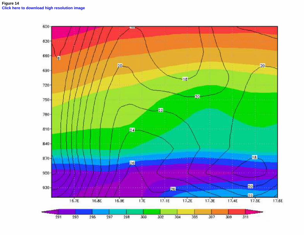
Figure 14Click here to download high resolution image

Table 1: MSG SEVIRI Spectral channel definition (EUMETSAT Format Guide v5a).

Channel

Number

Channel

Name

Bands Centre

wavelength

(μm)

Spectral Band

(99% energy limits)

(μm)

1 VIS0.6 Visible 0.635 0.56 - 0.71

2 VIS0.8 Visible 0.81 0.74 - 0.88

3 IR1.6 Near-infrared 1.64 1.50 - 1.78

4 IR3.9 Window 3.92 3.48 - 4.36

5 WV6.2 Water-vapour 6.25 5.35 - 7.15

6 WV7.3 Water-vapour 7.35 6.85 - 7.85

7 IR8.7 Window 8.70 8.30 - 9.10

8 IR9.7 Ozone 9.66 9.38 - 9.94

9 IR10.8 Window 10.80 9.80 - 11.80

10 IR12.0 Window 12.00 11.00 - 13.00

11 IR13.4 Carbon dioxide 13.40 12.40 - 14.40

12 HRV Visible (Broad

band)

0.75 0.6 - 0.9

Table 1

Table 2: List of LVD variables derived from satellite channels.

LVD

variable

name

Content description

GOES

centre

wavelength

(μm)

GOES

channel

Closest

MSG-SEVIRI

channel

SVS visible satellite - raw 0.6 1 1

SVN visible satellite -

normalized 0.6 1 1

ALB albedo 0.6 1 1

S3A bright temp averaged 3.9 2 4

S3C bright temp filtered 3.9 2 4

S4A bright temp averaged 6.7 3 5

S4C bright temp filtered 6.7 3 5

S5A unused

S5C unused

S8A bright temp averaged 11.2 4 9

S8W bright temp warmest

pixel 11.2 4 9

S8C bright temp coldest

pixel 11.2 4 9

SCA bright temp averaged 12.0 5 10

SCC bright temp averaged 12.0 5 10

Table 2

Table 3: Contingency table prototype.

Cloudy pixels for LAPS/SAFNWC SAFNWC cloudy SAFNWC no cloudy

Laps cloudy A B

Laps no cloudy C D

Table 3

Table 4: Spatial comparison index of cloud cover.

Time step/indexes BIAS PC

0900 1.059571 0.896936

1200 1.016894 0.915925

1500 1.147280 0.823943

Table 4

Figure captionsClick here to download Supplementary Material: Figure_captions.doc

Table captionsClick here to download Supplementary Material: Table_captions.doc