Using reduced data sets ISCCP-B2 from the Meteosat satellites to assess surface solar irradiance

Assessing Surface Solar Irradiance From ISCCP-B2 Data Sets

Lefèvre M., Diabaté L., Wald L., Using reduced data sets ISCCP-B2 from the Meteosat satellites to assess surface surface solar irradiance. Solar Energy, 81, 240-253, 2007, doi:10.1016/j.solener.2006.03.008.

USING REDUCED DATA SETS ISCCP-B2 FROM THE METEOSAT

SATELLITES TO ASSESS SURFACE SOLAR IRRADIANCE

M. Lefèvre (1), L. Wald (1), L. Diabaté (2)

(1) Centre Energétique et Procédés, Ecole des Mines de Paris / Armines, BP 207, 06904,

Sophia Antipolis cedex, France

(2) UFAE / GCMI, BP E4018, 410, avenue Van Vollenhoven, Bamako, Mali

Corresponding author: Lucien Wald, [email protected]

ABSTRACT

This paper explores the capabilities of a combination of the reduced data set ISCCP-B2 from

the Meteosat satellites and the recently developed method Heliosat-2 to assess the daily mean

of the surface solar irradiance at any geographical site in Europe and Africa. Firstly, we

discuss the implementation of the method Heliosat-2. Secondly, B2-derived irradiances are

compared to coincident measurements made in meteorological networks for 90 stations from

1994 to 1997. Bias is less than 1 W m-² for the whole set. Larger bias may be observed at

individual sites, ranging from -15 to +32 W m-². For the whole set, the root mean square

difference is 35 W m-² (17%) for daily mean irradiance and 25 W m-² (12%) for monthly

mean irradiance. These accuracies are close to those of similar data sets of irradiance, such as

Medias and NASA Surface Radiation Budget. It is concluded that B2 data can be used in a

reliable way to produce long-term time-series of irradiance for Europe, Africa and the

Atlantic Ocean.

Keywords: Satellite, radiation, fluxes, climatology, Africa, Europe, Atlantic Ocean

1

hal-0

0363

664,

ver

sion

1 -

24 F

eb 2

009

Author manuscript, published in "Solar Energy 81 (2007) 240-253" DOI : 10.1016/j.solener.2006.03.008

http://dx.doi.org/10.1016/j.solener.2006.03.008

http://hal.archives-ouvertes.fr/hal-00363664/fr/

http://hal.archives-ouvertes.fr


1. NOMENCLATURE

t time.

θS sun zenithal angle for the pixel under concern (radian)

θSnoon sun zenithal angle at noon for the pixel under concern (radian)

θV satellite viewing angle, formed by the normal to the ground and the direction of the

satellite for the pixel under concern. It is the complement to 90° of the satellite

altitude angle above horizon (radian)

TL Linke turbidity factor for a relative air mass equal to 2 (unitless)

I irradiance observed at ground level on horizontal plane, called SSI (surface solar

irradiance) (W m-2)

Id as I but averaged over one day (W m-2)

Ic SSI under very clear skies (W m-2)

Icd as Ic but averaged over one day (W m-2)

Kc clear-sky index. It is equal to the ratio of I to Ic (unitless)

KT clearness index. It is equal to the ratio of I to the irradiance observed outside the

atmosphere (unitless)

ρ t reflectance observed by the spaceborne sensor at instant t (unitless)

ρα t apparent reflectance of the ground at instant t (unitless)

ρeff effective reflectance of the brightest clouds (unitless)

ρcloud apparent cloud albedo observed by the spaceborne sensor over the brightest clouds

(unitless). It is a quantity specific to the method Heliosat

ρg ground reflectance (unitless)

ρgref reference ground reflectance (unitless)

ρatm intrinsic reflectance of the clear atmosphere (unitless)

T transmittance of the clear atmosphere (unitless)

n cloud index (unitless)

ΦP, ΦX latitude of respectively a point P, a point X (decimal degrees)

dgeo geodetic distance (km)

deff effective distance (km)

2

hal-0

0363

664,

ver

sion

1 -

24 F

eb 2

009


fNS a unitless parameter for interpolation taking into account the latitudinal asymmetry

of the climate phenomena

δh difference in elevation between the point P and another site X (km)

foro a unitless parameter for interpolation taking into account the difference in elevation

(=500)

2. INTRODUCTION

This paper deals with the assessment of the irradiance observed at ground level on horizontal

surfaces, also called surface solar irradiance (SSI). Accurate assessments can now be drawn

from satellite data, especially from the geostationary meteorological satellites such as

Meteosat covering Europe and Africa. Several studies demonstrate the superiority of the use

of satellite data over interpolation methods applied to measurements performed within a

radiometric network (Perez et al., 1997; Zelenka et al., 1992, 1999). Based on satellite data,

the project Surface Radiation Budget (SRB) is offering accurate monthly means of SSI for

several years and the whole Earth with a low spatial resolution (Whitlock et al., 1995; Darnell

et al., 1996). However, there is a demand for more detailed information in space and time

with an emphasis for long-term time-series of irradiance. Several atlases, digital or not, were

produced offering spatial resolutions better than 1° of arc angle: Raschke et al. (1991),

Medias (1996) and ESRA (2000). Several national weather bureaus are currently using

satellite data to map the SSI, e.g., Hungary (Rimoczi-Paal et al., 1999) or Australia (AGSRA,

2003). These initiatives do not fully answer the demand because they cover a limited area or a

limited period.

One obstacle to the production of such information is the large amount of data to process.

Take the example of the satellite system within the Meteosat Operational Programme (MOP).

One third of the Earth is imaged every 0.5 h in a broadband range (0.4 – 1.1 micron) with a

pixel size of 2.5 km at nadir. This creates an image of 5000 x 5000 pixels. A data set of

reduced spatial resolution, called ISCCP-B2 data, was created for the International Satellite

Cloud Climatology Project (ISCCP) to better handle and exploit this wealth of information

(Schiffer and Rossow, 1985). If one keeps only the pixels that can be processed to produce

SSI, i.e., approximately 70% of the whole image, one year of data means approximately a

volume of 243 Gigabytes for high-resolution data and 0.2 only for B2 data. Using B2 data

permits very large gains in data storage, especially when contemplating the creation of an

archive of 20 years or more as we do. In addition, B2 data were cheaper than high-resolution

3

hal-0

0363

664,

ver

sion

1 -

24 F

eb 2

009


data, at least for Meteosat satellites and before the latest changes in data policy of Eumetsat,

the owner of the Meteosat data. For example, ten years ago, when our project started, one

year of high-resolution data was more than 20 keuro worth while the cost was only 500 euro

for B2 data. This was the second reason for choosing B2 data. Figure 1 displays an example

of a B2 image for Meteosat.

Several authors already used B2 data for the assessment of the SSI (Ba et al., 2001; Raschke

et al., 1987; Tuzet et al., 1984). These works clearly demonstrated the interest of B2 data for

producing long-term time-series of SSI over large periods. However, the assessment of the

quality of the B2-derived SSI is limited in these papers in the number of sites and period of

time. This paper addresses this problem. It explores the capabilities of a combination of the

B2 data set and the recently developed method Heliosat-2 to assess the SSI at any

geographical site in Europe and Africa. In addition, it describes the operational

implementation of the method Heliosat-2. This implementation was performed by using the

software libraries that are freely available at the web site www.helioclim.net.

3. THE METHOD HELIOSAT-2 AND ITS IMPLEMENTATION

The model for converting satellite data into SSI is the method Heliosat-2 proposed by

Rigollier et al. (2004, abbreviated RLW in the following). This method is particularly suitable

for processing time-series of data acquired by a series of sensors that are similar but differ

slightly in calibration as it is the case of the Meteosat system prior to 1998 (Anonymous

1996). It is based on the principle that the attenuation of the downwelling shortwave radiation

by the atmosphere over a pixel is determined by the magnitude of change between the

reflectance that should be observed under a very clear sky and that currently observed (Pastre,

1981; Cano et al., 1986; Stuhlmann et al., 1990). In the method Heliosat-2, the SSI is

computed by the means of the clear-sky index Kc defined as:

Kc = I / Ic (1)

where Ic is the SSI under clear skies. The clear-sky index Kc is derived from the satellite

images as explained later. Ic is modelled by a clear-sky model. Two other quantities are

instrumental in this method: the reflectance of the ground (also called the ground albedo) and

that of very reflective clouds.

3.1 The clear-sky model

4

hal-0

0363

664,

ver

sion

1 -

24 F

eb 2

009


The clear-sky model provides Ic. RLW discuss the choice of the ESRA model (Rigollier et al.,

2000). The inputs to this model are the solar zenithal angle θS, the elevation of the site and the

Linke turbidity factor for a relative air mass 2, TL. The database TerrainBase (1995) is

adopted for elevation; it contains the mean elevation for each cell of 5’ of arc angle

worldwide. The Linke turbidity factor TL is a very convenient approximation to model the

atmospheric absorption and scattering of the solar radiation under clear skies. It describes the

optical thickness of the atmosphere due to both the absorption by the water vapour and the

absorption and scattering by the aerosols relative to a dry and clean atmosphere. Like the

water vapour and the aerosol optical parameters, TL is known at a limited number of sites. It

greatly varies in space and in time. Remund et al. (2003) collected a number of observed

values of TL worldwide and merged these values with gridded maps of TL derived from the

ISCCP clear-sky SSI at coarse resolution (approx. 300 km), other maps of water vapour and

aerosol optical properties and the database TerrainBase. The fusion of these various sets of

data created a series of 12 maps, one per month, covering the world with a cell of 5’

(approximately 10 km at mid-latitude).

This database of TL is available from Les Presses, Ecole des Mines de Paris, and we use it as

an input. There is one value per month; time interpolation is performed for each day. As these

are typical values of TL for a month, the discrepancies between the database and the actual

values lead to errors in assessing the SSI as indicated by Eq. 1. TL may vary greatly from one

hour to another, or one day to another. It is often set to 3.5 in Europe as an average but large

variations may be observed from 2.5 to 5 typically in urban areas with heavy vehicle traffic

between early morning when there is no pollution and the afternoon with pollution at its

maximum. According to graphs in Rigollier et al. (2000), a change of 1 in TL leads to a

relative change of approximately 10 – 15% in Ic and thus in I. The sensitivity of the outcomes

of the method Heliosat-2 to TL is studied by RLW by the means of a comparison with one

year of ground measurements made at 35 sites in Europe. By setting TL to typical values for

each site and then to a fixed value of 3.5, RLW found that the bias between measured SSI and

Heliosat-2-derived SSI is sensitive to the selected values of TL. The largest discrepancies are

found when the sun is low above the horizon. RLW note that the influence is not limited to

clear-sky cases. Besides this source of error, we should mention that the database exhibits

exaggerated spatial gradients that were created artificially by the fusion process. These

gradients will appear in the resulting SSI maps (Eq. 1) and this is another source of error.

Nevertheless, this database is the only source we know of TL for every pixel of the Meteosat

images and this is a good reason to use it.

5

hal-0

0363

664,

ver

sion

1 -

24 F

eb 2

009


Using this ESRA model, RLW compute the intrinsic reflectance of the atmosphere, ρatm, the

downward (sun to ground) and upward (ground to satellite) transmittances of the clear

atmosphere T(θS) and T(θV), where θV is the satellite viewing angle, formed by the normal to

the ground and the direction of the satellite. By comparison with radiative transfer models and

ground measurements, RLW find that the accuracy in the retrieval of these quantities

degrades for θS or θv greater than 75°. They recommend to not using the method Heliosat-2

for such angles.

3.2 The reflectance of the ground

Under clear skies, the actual reflectance of the ground, ρg, is approximately equal to:

ρg = [ ρ t - ρatm] / T(θS) T(θv) (2)

where ρ t is the reflectance observed by the spaceborne sensor at instant t. Since we do not

know a priori which pixels and instants are cloud-free, we apply Eq. 2 to a time-series of

observed reflectances and we obtain a time series of possible ground reflectances, called

apparent ground reflectances ρα t. The time-series is constructed by taking all images available

for a month. Assuming that at a given location, the ground reflectance is less than the

reflectance of any cloud and that the ground reflectance is constant throughout the month, the

ground reflectance at this location is in principle the minimum value in this time-series. The

time-series for a pixel is restricted to instants for which the sun is high enough above the

horizon:

θS ≤ minimum( 2 [π/2 − θ Snoon] / 3, 5π/18 ) (3)

where θSnoon is the angle observed at noon. The first and second minima are searched in this

time series. Experience shows that the absolute minimum is subject to undetected defects in

the original image or to other processes, such as shadows of clouds, which create artificially

low ground reflectances, especially in desert areas, and is more variable than the second

minimum. Therefore, we set the ground albedo ρg for this period to the second minimum.

Note that this does not ensure that this value is the requested ground reflectance: it may be a

cloud reflectance if all instants are cloudy or if ρg is larger than the lowest reflectances of

clouds, or the shadow of a cloud or a minimum of ρg if the latter varies during the month. One

way to palliate this shortcoming may be to consider the same time-series but in the thermal

infrared range. The radiances observed in this range are a function of the temperature of the

6

hal-0

0363

664,

ver

sion

1 -

24 F

eb 2

009


object. If one assumes that the ground is warmer than any cloud, one may search the instant

when temperature reaches its maximum and decide that ρg is equal to the reflectance for this

instant. Another solution may be to search for local extreme in bidimensional space: low

reflectance and high temperature.

In our case, only images in visible band were available. Before performing the search for ρg

for every month, we perform this operation once for all for a time-series of images spanning

from 1985 to 1990. Only images acquired at 1200 UTC were used; at that time most pixels

are well sunlit. The resulting ground albedo was checked against typical values for soils

(urban areas, vegetated fields), forests, deserts and water (Moussu et al., 1989) with the help

of atlases and maps. Corrections to the ground albedo were brought manually if necessary;

they concerned pixels which are the farthest from the nadir point of the satellite which is

located in the equatorial plane at 0° in longitude or which are in the equatorial areas

permanently covered by clouds. Thus, we created a map of ground albedo that include

external knowledge and that is called reference map, ρgref. This map is used to control the

ground reflectance assessed every month: ρg should be comprised in the interval [ρgref /2, 2

ρgref]. Otherwise, it is set to the corresponding threshold. The use of a reference map prevents

the case of geographical areas that are under clouds for long periods, such as the equatorial

belt or some parts of Northern Europe.

The authors are aware that this approach to the ground albedo is limited as already discussed

by RLW. It cannot cope with the case of a sudden appearance of snow on the ground, a case

which occur frequently in winter in Europe; the impact on the retrieval of the SSI is usually

small because the sky is fully overcast but if not, the error in retrieval may be very large as it

was the case in winter 2005. The assessment of the ground albedo may be improved by

integrating the work of Zelenka (2003). In a similar way, one may consider shortening the

period from one month to one week in order to deal with the rapid appearance of vegetation in

Sahelian regions (Diabaté et al., 1989). Indeed, a trade-off should be found between the time

requested to have a cloud-free instant for sure and the time scale of the rapid changes in

albedo. Such an investigation has not yet been performed in our group; it is possible that the

solution proposed for snow appearance may work in other cases.

Beyond these spectacular cases, one should note the importance of the assessment of the

ground reflectance on the error in the assessment of the SSI. This is illustrated by a rough

computation. If we restrict ourselves to the case where the clear-sky index ranges from clear

(Kc =1) to slightly overcast (Kc =0.2), the equations of the method Heliosat-2 (see below) lead

7

hal-0

0363

664,

ver

sion

1 -

24 F

eb 2

009


to:

Kc = 1 - [ρα t - ρg ] / [ρcloud - ρg ] (4)

where ρcloud is the reflectance of the very reflective clouds. Assume that the actual value of

the ground reflectance is ρg. Its estimate, ρg*, differs by ε

ρg* = ρg + ε (5)

The estimate Kc* differs from the actual value:

Kc* = Kc + (ε / ρcloud ) (6)

and the estimate I* of the SSI:

I* = I + Ic (ε / ρcloud ) (7)

Eq. 7 shows that an error in ρg, positive or negative, leads to an error in I of the same sign.

This error does not depend on the cloud cover. Its relative influence is the greatest for

overcast skies. This error is actually not a bias because it depends upon ρcloud that is itself a

function of θS and θv as explained below. Nevertheless, for a given pixel, i.e. a given θv, if we

assume that θS exhibits small changes throughout the month for a given hour, one may

consider this error as a bias in the SSI. Typical values for ε and ρcloud are respectively, 0.05

and 1.5. The error is then 0.03 times Ic. In the case of Northern Europe where clouds are very

frequent, a typical clear-sky SSI is 300 W m-² and I is 100 W m-²; consequently, the error

would be 9 W m-², i.e., 9% of I.

3.3 The reflectance of the very reflective clouds

RLW assessed the effective reflectance of very reflective clouds ρeff from drawings in Taylor

and Stowe (1984a):

ρeff = 0.85 –0.13 [1 - exp(−4 cos(θS)5] (8)

Note that a mistake was made in the corresponding equation in RLW (Eq. 8, 0.78 was written

instead of 0.85). To compare the cloud reflectance to the ground reflectance, RLW define

ρcloud as:

ρcloud = [ ρeff - ρatm] / T(θS) T(θv) (9)

with

ρcloud > 0.2, otherwise ρcloud = 0.2 and

ρcloud < 2.24 ρeff, otherwise ρcloud = 2.24 ρeff

8

hal-0

0363

664,

ver

sion

1 -

24 F

eb 2

009


The value 2.24 is the largest anisotropy factor observed by Taylor and Stowe (1984b) for the

geometrical configuration sun-pixel-Meteosat and thick water cloud. A typical value for ρcloud

is 1.5. As for ρg, we can assess the influence of an error in ρcloud on I. Assume that Kc is in the

range [0.2, 1] and that ρcloud is much greater than ρg. Then, we can write:

Kc ≈ 1 – (ρα t - ρg ) / ρcloud (10)

Assume ρcloud is the actual value for very reflective clouds. Its estimate, ρcloud*, differs by a

quantity δ such as:

ρcloud* = ρcloud (1+ δ) (11)

with δ ≥ 0 or < 0 and ABS(δ) << ρcloud

where ABS means the absolute value. The estimate Kc* of Kc is:

Kc* ≈ 1 – (ρα t - ρg ) / ρcloud*

= 1 – (ρα t - ρg ) / [ρcloud (1+ δ)] (12)

Kc* ≈ 1 - [(ρα t - ρg ) / ρcloud ] (1- δ)

≈ Kc + (1 – Kc) δ (13)

The estimate I* of I is:

I* = Kc* Ic ≈ Kc Ic + (1-Kc) δ Ic

= I + (1-Kc) δ Ic (14)

The error in I is (1-Kc) δ Ic; it has the same sign that δ. It is equal to 0 when Kc=1. It increases

as Kc decreases, i.e., as the sky is becoming cloudy. It may be very large as shown by the

following numerical example. Assume δ = 0.25 and Kc = 0.2. Then the error is equal to 20%

of Ic. If we take the same case as before with Ic = 300 W m-² and I = 100 W m-², the error

amounts to 60 W m-², that is 60% of I.

3.4 The computation of the daily mean of SSI

For each pixel and each instant, a cloud index n t is computed:

n t = [ρα t - ρg

t ] / [ρcloud t - ρgt ] (15)

The cloud index is close to 0 when the observed reflectance is close to the ground reflectance,

i.e., when the sky is clear. It can be negative if the sky is very clean, in which case ρα t is

smaller than ρgt. The cloud index increases as the clouds are appearing. It can be greater than

9

hal-0

0363

664,

ver

sion

1 -

24 F

eb 2

009


1 for clouds that are considerably optically thick. Compared to RLW, we add several

numerical constraints and the cloud index is computed as follows:

If ρα t < 0.01, n t = 0

Else if ABS(ρα t - ρg

t ) < 0.01, n = 0

Else if ABS(ρcloud t - ρgt ) < 0.10, n = 1.2 (an arbitrary large value)

Else n t = [ρα t - ρg

t ] / [ρcloud t - ρgt ] (16)

If n t < -0.5, n t =-0.5

If n t > 1.5, n t = 1.5

An example of an image of cloud index is given in Fig. 2. The following relationship holds

between nt and Kc:

nt < -0.2 Kc = 1.2 -0.2 < nt < 0.8 Kc = 1 - nt (17) 0.8 < nt < 1.1 Kc = 2.0667 - 3.6667 nt + 1.6667(nt)²

nt > 1.1 Kc = 0.05 Then, the SSI I t is computed for this instant t by the means of Eq. 1. The daily mean of SSI Id

is computed from the N values of I t available for that day:

Id = ∑ / N (18) =

N

1i

iI

At each instant in the summation, θS should be smaller than 75° for the clear-sky model to be

valid. The larger N, the more accurate Id. In our case, where B2 data are used, N ranges from

1 to 5.

Thus, the method Heliosat-2 converts satellite data into assessments of the daily mean of the

SSI for each day. The accuracy of the method was assessed by RLW by processing high-

resolution Meteosat images and comparing the derived SSI to measurements made in the

meteorological networks in Europe. The results of RLW are reproduced in Table 1. Note that

contrary to many similar works, these values are obtained by comparing the ground

measurements to the estimated values for the single pixel containing the ground station with

no spatial averaging.

3.5 The special case of the sun glitter over the ocean

The pattern of dancing highlights caused by the reflection of the sun from a water surface is

called the sun glitter pattern. The surface of the ocean may be differentiated into small, mirror

like facets. At spacecraft altitude, the reflecting facets are not individually resolved.

10

hal-0

0363

664,

ver

sion

1 -

24 F

eb 2

009


Therefore, the apparent radiance of the sea surface in any direction depends on the fraction of

the area having the proper slope for specular reflection. The observed glitter pattern shows a

radiance decreasing smoothly outward from its centre, since greater and therefore less

frequent slopes are required for specular reflection as the distance from the centre increases

(Wald and Monget, 1983a). This is illustrated in Fig. 1. When the wind speed increases, the

roughness of the sea surface increases, the occurrence of large facet slopes increases and the

pattern broadens with the level of radiance at the centre decreasing. The glitter pattern is

centred on the specular point that is approximately defined as the pixel for which the satellite

viewing and solar zenithal angles are equal and the difference of the azimuths of the sun and

the satellite is equal to 180 ° (they are opposite). Far from the specular point, the ocean

reflectance is approximately constant. In Fig. 1, the glitter pattern is visible in the middle of

the image; the sun is at its zenith; the specular point is roughly southward of the nadir of the

satellite.

Contrary to the usual case of ground reflectance, the reflectance of the ocean is highly

variable with θS, θV and the difference in azimuth angles of the sun and sensor because of its

non-Lambertian nature; it ranges from null values to values greater than cloud reflectances

(Wald and Monget, 1983b). In addition, it depends upon the instantaneous wind speed at the

surface. The approach adopted to assess the ground albedo is not effective in the case of the

glitter pattern. It is suitable only outside this area. Another approach was designed within the

glitter pattern. For practical reasons, it was decided to correct the cloud index in the glitter

pattern instead of the reflectance. A window is defined centred on the specular point. The

search for this point is limited to the area where it can be observed, i.e. between the latitudes

35° N and –35° S approximately, with θS and θV less than 40°. Otherwise, no correction is

applied. The window is large enough to encompass the largest size of the glitter pattern:

approximately 2000 km in radius. Only are considered the pixels known as belonging to the

ocean. For each pixel in this window, if the cloud index is greater than 0.2, the sky is said

cloudy and no correction is applied. Otherwise, a new window of 3 x 3 pixels is defined

centred on the current pixel. One counts the number of pixels exhibiting cloud indices less

than 0.2. If this number is strictly greater than 5 (60% of the total), the current pixel is

considered as cloud-free and the cloud index is set to 0. Figure 2 shows the application of the

method on the previous image (Fig. 1). The uncorrected map exhibits cloud indices that are

too large in the glitter pattern. They are mistaken as clouds and the resulting SSI will be too

low. Once corrected, the cloud indices offer values that are similar to the other cloudless parts

of the ocean. The cloudy pixels are not affected by the correction.

11

hal-0

0363

664,

ver

sion

1 -

24 F

eb 2

009


4. THE B2 DATA SET USED

The B2 data set is produced from Meteosat images by firstly performing a time sampling that

reduces the frequency of observation to the standard meteorological synoptic 3-h intervals,

starting at 0000 UTC. The Earth is scanned by the first series of Meteosat satellites

(Meteosat-1 to –7) in approximately 25 minutes. An image acquired at, say 1200 UTC is

actually acquired between 1130 and 1155 UTC. The time used in the computations is the

actual acquisition time for this particular pixel. Secondly, the higher-resolution data in the

visible-channel are averaged to match the lower resolution of infrared-channel data (i.e. an

image of 2500 x 2500 pixels with a resolution of 5 km). Finally, a spatial sampling is

performed by taking 1 pixel over 6 in each direction, starting with the south-easternmost

pixel. The effects of the temporal sampling on the reconstruction of the daily mean of SSI

were discussed by England and Hunt (1984); they found that the accuracy decreases as the

sampling rate decreases. Pinker and Laszlo (1991) investigated the effects of spatial sampling:

the estimated SSIs differed by 9% depending upon the sampling. Consequently, we expect a

lower accuracy for the SSI derived from B2 data than for those derived from high-resolution

images (Table 1).

The B2 data set spans from 1994 to 1997. It covers the whole field of view of Meteosat, i.e.

Europe, Africa and the Atlantic Ocean. Meteosat data were converted into radiances using the

calibration coefficients proposed by Rigollier et al. (2002). Each image of radiances was

processed by the means of the method Heliosat-2. Estimates of the daily mean of SSI are thus

obtained for each B2 pixel. There are 118500 such pixels. The assessment of the SSI for any

geographical site P is made by the means of a linear interpolator of gravity-type applied to the

nine nearest B2 pixels Xj (j=1…9):

Id(P) = )(I9

1jjdj Xw∑

= (19)

where Id(Xj) denotes the SSI at B2 pixel Xj. The weights wj are defined by the inverse of a

squared distance dj separating P and each Xj:

wj = (1 / dj2) ∑

=

9

1k

2dk (20)

The geodetic distance between P and Xj ranges from 20 to 80 km. After several comparisons

with the nearest neighbour and the geodetic distance, we selected the effective distance

12

hal-0

0363

664,

ver

sion

1 -

24 F

eb 2

009


proposed by Lefèvre et al. (2002) and already used by Diabaté et al. (2004) for mapping solar

radiation climate in Africa. This effective distance deff takes into account latitudinal and

orographic effects and offers a better accuracy:

(deffj)2 = (fNS

j)2 ((dgeoj)2 + foro

2 (δhj)2) (21)

with (fNSj) = 1 + 0.3 ABS(ΦP -ΦXj) [1+ (sinΦP + sinΦXj) / 2]

where (dgeoj) is the geodetic distance between P and Xj in km, latitudes ΦP and ΦXj are

expressed in degrees, counted positive from the equatorial plane northwards and negative

southwards, (δhj) is the difference in elevation between P and Xj, expressed in km, and foro is

equal to 500.

5. COMPARING GROUND MEASUREMENTS TO SATELLITE-DERIVED

ASSESSMENTS

Ground measurements were assembled to assess the B2-derived SSI. They consist in daily

irradiation collected by the meteorological networks in Europe and Africa. Fifty-five stations

are available for Europe, covering July 1994 to June 1995, and located in flat areas of low

altitude (Table 2). Thirty-five stations are available for Africa, covering four years, spanning

from January 1994 to December 1997 (Table 3). The quality of the ground data measurements

of the global irradiation was controlled by the means of a Web tool in order to remove

suspicious data (see at www.helioclim.net, Geiger et al., 2002). Following the ISO standard

(1995), we compute the difference: estimated-measured for each day, and summarize these

differences by the bias, the root mean square difference (RMSD) and the correlation

coefficient. We performed this operation for daily and monthly means of SSI, each region and

each year. The monthly means are computed from daily values; we kept only days that are

coincident in both time-series and declared a monthly mean valid only if it is made from at

least 60% of valid daily mean of SSI, i.e., 17 to 18 days per month.

The authors consider that the result of the interpolation procedure is equivalent to an

assessment made over a pixel containing the site P. Therefore, the two time-series to compare

are different in nature: one is made of pin-point measurements, the other of space-averaged

assessments. Accordingly, a discrepancy is expected because of the natural variability of the

SSI in space; Zelenka et al. (1999) found within a pixel a standard deviation of 10-15%

relative to the mean SSI.

13

hal-0

0363

664,

ver

sion

1 -

24 F

eb 2

009


Table 4 reports results for the daily mean of SSI. The correlation coefficient is high in all

cases and larger than 0.9: day-to-day variations are well reproduced. Looking for Europe, one

note that the bias and RMSD are close to those reported in Table 1 for high-resolution

imagery. The bias is negative, which means an underestimation of the SSI. As expected, the

bias and RMSD are greater than those found by RLW with high resolution images, and the

differences in RMSD are in agreement with the findings of England and Hunt (1984) and

Pinker and Laszlo (1991). As a whole, the bias is negative for Europe (underestimation) and

positive for Africa (overestimation). The bias varies from one year to another. It is of order of

a few percent in relative value though a large value of 9% was found for Europe in 1995. The

relative RMSD ranges between 15 and 25%. The largest relative difference is attained for

Europe in 1995 and is related to the largest relative bias.

If all data are merged together, the observed mean value is 202 W m-², and with 48490

observations spanning from 1994 to 1997, we found a bias of 1 W m-², which is very low; the

RMSD is 35 W m-² (17%).

However, the picture is not as simple if we consider sites individually. The bias may range

from –15 W m-² (Easthampstead, United Kingdom) to 32 W m-² (Wenchi, Ghana). Though

for Europe, the bias is negative, it is equal to 8 W m-² in Bergen (Norway) for 1994-1995. On

the contrary, we found a bias of –13 W m-² in Bahtim (Egypt) or Nampula (Mozambique)

while the overall bias for Africa is positive. The study indicates that the relative bias and

relative RMSD are usually low for clear skies and degrade for overcast skies but this is only a

trend as it will be illustrated later. As a whole the greater the irradiance, the greater the bias in

absolute value and the greater the RMSD. This was observed by RLW (Table 1). For Europe,

it means that error in January is less than in July. Combined to that, one may observe in

general a seasonal variation in error at a given site (Figs 3 to 6). This is not true for all sites

(Fig. 3). The sun elevation plays a role; an overestimation of the SSI is often observed for low

sun elevation (large θS). One of the possible reasons is the decrease in the number N of hourly

estimates for constructing the daily mean (Eq. 18). The influence of θV is not noticeable.

Nevertheless, it is difficult to draw definite conclusions as there are several quantities in the

method Heliosat-2 that influence the results as already discussed and illustrated below.

The correlation coefficient for monthly mean of SSI is higher than for the daily mean of SSI

(Table 5). The relative RMSD ranges between 11 to 13% with an exception at 16% for

Europe in 1995. If all data are merged together (1584 samples), the bias is 1 W m-² and the

RMSD is 25 W m-² (12%), notably less than for the daily mean of SSI.

We selected four stations to illustrate the quality and drawbacks of the method. These four

14

hal-0

0363

664,

ver

sion

1 -

24 F

eb 2

009


stations are representative of a radiation climate according to ESRA (2000) and Diabaté et al.

(2004). Braunschweig, in Germany, is situated at the northern foot of the central German

uplands. The station is influenced partly by maritime but more by continental air masses

depending on the actual weather conditions. Classified with the climatic types of Trewartha

(1954), the area has a climate coded as Cb: rainy climate with mild winters, coldest month

with mean temperatures ranging between 0 and 8° C, warmest month with mean temperatures

less than 22° C. The average clearness index KT is reported for each month in Table 6.

Wenchi is located in Ghana in the equatorial zone, North of the Gulf of Guinea. The climate is

coded Aw, which means a rainy climate with no winter and the driest months in boreal winter.

The temperature of the coolest month is above 18° C. KT is almost constant from November to

May at approximately 0.45 (Table 6). Then it decreases to 0.32 in August and then increases

again. Maputo (Mozambique) is located on the Southeast coast of Africa, in the Limpopo

plain. The climate is similar to that of Wenchi (code Aw) with the driest months in austral

winter (June-August). It is characterized by KT almost constant during the year, ranging

between 0.53 and 0.59, with a maximum in austral winter (Table 6). El Arish is in the arid

Sinai Peninsula. Climate is that of a warm dry desert (code BWh). The sky is very clear in

boreal summer: KT is larger than 0.65 (Table 6). The lowest values of 0.55 are attained in

November and December.

Figure 3 displays the monthly means of SSI observed and assessed at Braunschweig. Table 7

reports on the statistics for this site. The underestimation is important: -13 W m-²; the RMSD

is slightly greater than the bias, in absolute value; the correlation coefficient is very large:

0.99. The assessed SSI reproduces quite well the variations of the observed SSI, except for

July 1995. The underestimation may be explained by TL slightly too large (i.e. Ic too small)

from January to June as explained by Equation 1. The outlier seen for July 1995 is due to an

underestimation of ρg; it may be due to an optically thin cloud that decreases the reflectance

of the ground observed by the sensor. Equation 7 shows that an underestimation of ρg leads to

an underestimation of the SSI. For the site Wenchi (Fig. 4, Table 7), the agreement is not

good. The correlation coefficient is lower than usual: 0.77. There is a large overestimation

from November to April that can be explained by too low values of TL (i.e. Ic too large). The

agreement in austral winter (June-August) is fairly good in 1994 and very good in 1995

though the sky is very cloudy during this period. This illustrates the fact that though the

relative error usually increases when the cloud cover increases, it is not systematically the

case. The agreement is very good for the site Maputo (Fig. 5, Table 7). The correlation

coefficient is very large: 0.96; the bias and RMSD are small. A large underestimation (-50 W

15

hal-0

0363

664,

ver

sion

1 -

24 F

eb 2

009


m-²) is observed in February 1994. As the SSI is very similar from one year to another and as

the agreement is good for February 1995, we conclude that TL is correct and that the

discrepancy in February 1994 is likely due to an underestimation of ρg. The site El Arish

exhibits one of the best agreements (Fig. 6 and Table 7). The correlation coefficient is 1.00

and the bias is low. One may observe an overestimation in June-July and an underestimation

in November-December for both years. As the SSI is constant from one year to another, we

may conclude that TL should be modified for these 4 months.

6. CONCLUSION

With an observed mean value of 202 W m-², we found a bias of 1 W m-² and a RMSD of 35

W m-² (17%) for daily mean of SSI. This is slightly worse than the accuracy reported for the

data set Medias (1996) that deals with the Mediterranean basin. The Medias data set was

constructed using original Meteosat data, with a temporal sampling of 0.5 h and a degraded

spatial resolution of 0.2° of arc angle (approximately 20 km). A comparison made against

9116 observations made in France in 1994, with a mean value of 145 W m-², results into a

bias of -1 W m-² and a RMSD of 18 W m-² (13%). These values are similar to those found by

RLW; the differences with the present study are related to the difference in temporal sampling

(0.5 h versus 3 h) and to the use of spatial averaging in the case of the Medias data set.

As for the monthly mean of SSI, we found of course a similar bias of 1 W m-² and a RMSD of

25 W m-² (12%). This is close to the accuracy of the SRB data set. Comparing irradiance on

pixel of 280 km in size and 13356 measurements made in the Global Energy Balance Archive

(GEBA) from July 1983 to June 1991, Darnell et al. (1996) report a bias of -5 W m-² and a

RMSD of 24 W m-².

The results clearly demonstrate that the combination of the images in reduced format B2 and

the method Heliosat-2 offers enough accuracy for creating a climatological database of the

daily mean SSI over large areas with a grid cell of about 5' of arc angle in size (approximately

10 km at mid-latitude). It is concluded that such B2 data can be used in a reliable way in

producing time-series of SSI for Europe, Africa and the Atlantic Ocean, except for very high

latitudes greater than approximately 65°. Though not tested, the authors believe that the

conclusions hold for other parts of the world.

An effort has been launched at Ecole des Mines de Paris / Armines for creating and managing

a database, called HelioClim-1, that contains daily mean of SSI for the field of view of

16

hal-0

0363

664,

ver

sion

1 -

24 F

eb 2

009


Meteosat for a period beginning 1st January 1985 (Cros, 2004; Cros et al., 2004). The data are

accessible via the SoDa Web site (http://www.soda-is.com). The database comprises the

equivalence of 118500 measuring pseudo-stations (the B2 pixels). Given any geographical

location, the Web server performs an on-line spatial interpolation using the nine surrounding

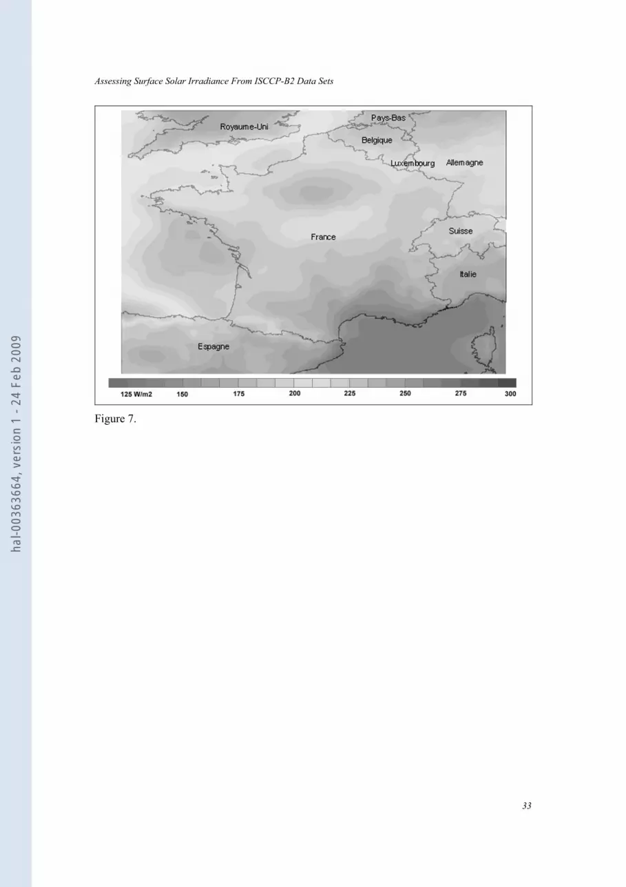
pseudo-stations to deliver a time-series of irradiance for this location. Figure 7 displays an

example of a map constructed from this database. It represents the monthly mean of SSI for

France and surroundings in August 2003. The grey scale was constructed in order to display

best the spatial features and to demonstrate that features of scale of 50 km or greater are well

represented.

In this geographical area (Europe, Africa), there are about 410 stations measuring the global

radiation on a daily basis in the WMO network (source WMO Web site www.wmo.ch, 3 May

2002). These 410 stations hardly compare to the 118500 pseudo-stations. There are in

addition 1910 WMO stations measuring the sunshine duration; the latter can be converted into

global radiation for monthly means if the parameters of the Angstrom relation between both

quantities are known. Even so, this number cannot compete against the capabilities offered by

the satellite, even in reduced format.

ACKNOWLEDGMENTS The World Radiation Data Center (WRDC) provided the data for Africa. The meteorological

offices from Belgium, France, Germany, Hungary, South Africa, Spain and United Kingdom

have kindly provided the measurements of global irradiation at no or low cost. They are

thanked for their support. Thanks to Jan Olseth for the data for Bergen, Norway. The B2 data

were offered at reproduction cost by Eumetsat. Many thanks go to the anonymous reviewers

whose comments help in greatly improving the quality of this article. This work was partly

supported by the European Commission, under the Information Society Technology

Programme (SoDa project IST-1999-12245) and partly by the Service de Coopération et

d'Action Culturelle de l'Ambassade de France in Mali.

REFERENCES AGSRA, Australian Global Solar Radiation Archive server, on-line at www.bom.gov.au,

2003.

Anonymous, 1996. The Meteosat system, Eumetsat publ. #TD05, Eumetsat, Darmstadt,

17

hal-0

0363

664,

ver

sion

1 -

24 F

eb 2

009


Germany.

Ba, M., Nicholson, S., Frouin, R., 2001. Satellite-derived surface radiation budget over the

African continent. Part II: Climatologies of the various components. Journal of Climate, 14,

60-76.

Cano, D., Monget, J.-M., Albuisson, M., Guillard, H., Regas, N., Wald, L., 1986. A method

for the determination of the global solar radiation from meteorological satellite data. Solar

Energy, 37, 31-39.

Cros, S., 2004. Création d’une climatologie du rayonnement solaire incident en ondes courtes

à l’aide d’images satellitales. Thèse de Doctorat en Energétique, Ecole des Mines de Paris,

Paris, France, 157 pp.

Cros, S., Albuisson, M., Lefèvre, M., Rigollier, C., Wald, L., 2004. HelioClim: a long-term

database on solar radiation for Europe and Africa. In Proceedings of Eurosun 2004, published

by PSE GmbH, Freiburg, Germany, pp. 916-920(3).

Darnell, W.L., Staylor, W.F., Ritchey, N.A., Gupta, S.K., Wilber, A.C., 1996. Surface

radiation budget: a long-term global dataset of shortwave and longwave fluxes, American

Geophysical Union. Available from: http://www.agu.org/eos_elec/95206e.html.

Diabaté, L., Michaud-Regas., N., Wald, L., 1989. Mapping the ground albedo of Western

Africa and its time evolution during 1984 using Meteosat visible data. Remote Sensing of

Environment, 27, 3, 211-222.

Diabaté, L., Blanc, Ph., Wald, L., 2004. Solar radiation climate in Africa. Solar Energy, 76,

733-744.

England, C.F., Hunt, G.E., 1984. A study of the errors due to temporal sampling of the earth's

radiation budget, Tellus, 36B, 303-316.

ESRA, 2000. European Solar Radiation Atlas, fourth ed., includ. CD-ROM. Edited by Greif,

J., and K. Scharmer. Scientific advisors: R. Dogniaux, J. K. Page. Authors: L. Wald, M.

Albuisson, G. Czeplak, B. Bourges, R. Aguiar, H. Lund, A. Joukoff, U. Terzenbach, H. G.

Beyer, E. P. Borisenko. Published for the Commission of the European Communities by

Presses de l'Ecole, Ecole des Mines de Paris, Paris, France.

Geiger, M., Diabaté, L., Ménard, L., Wald, L., 2002. A web service for controlling the quality

of measurements of global solar irradiation. Solar Energy, 73, 475-480.

ISO, 1995. Guide to the Expression of Uncertainty in Measurement, first ed. International

Organization for Standardization, Geneva, Switzerland.

Lefèvre, M., Remund, J., Albuisson, M., Wald, L., 2002. Study of effective distances for

interpolation schemes in meteorology. Geophysical Research Abstracts, 4, April 2002,

18

hal-0

0363

664,

ver

sion

1 -

24 F

eb 2

009

http://www.agu.org/eos_elec/95206e.html


EGS02-A-03429, European Geophysical Society.

Medias, 1996. Mediterranean Oceanic Database – Satellite Data and Meteorological Model

Outputs. 2 CD-ROMs, produced by Meteo-France, CNES, IFREMER, CLS, ESA and GRGS.

Published by Medias-France, CNES, Toulouse, France.

Moussu, G., Diabaté, L., Obrecht, D., Wald, L., 1989. A method for the mapping of the

apparent ground brightness using visible images from geostationary satellites. International

Journal of Remote Sensing, 10, 7, 1207-1225.

Pastre, C., 1981. Développement d’une méthode de détermination du rayonnement solaire

global à partir des données Meteosat. La Météorologie, VIe série N°24, mars.

Perez, R., Seals, R., Zelenka, A., 1997. Comparing satellite remote sensing and ground

network measurements for the production of site/time specific irradiance data. Solar Energy,

60, 89-96.

Pinker, R. T., Laszlo, I., 1991. Effects of spatial sampling of satellite data on derived surface

solar irradiance. Journal of Atmospheric and Oceanic Technology, 8, 96-107.

Raschke, E., Gratzki, A., Rieland, M., 1987. Estimates of global radiation at the ground from

the reduced data sets of the International Satellite Cloud Climatology Project. Journal of

Climate, 7, 205-213, 1987.

Raschke, E., Stuhlmann, R., Palz, W., Steemers, T.C., 1991. Solar Radiation Atlas of Africa,

published for the Commission of the European Communities by A. A. Balkema, ISBN 90-54-

5410, 155 pp.

Remund, J., Wald, L., Lefèvre, M., Ranchin, T., Page, J., 2003. Worldwide Linke turbidity

information. Proceedings of ISES Solar World Congress, 16-19 June 2003, Göteborg,

Sweden, CD-ROM published by International Solar Energy Society.

Rigollier, C., Bauer, O., Wald, L., 2000. On the clear sky model of the 4th European Solar

Radiation Atlas with respect to the Heliosat method. Solar Energy, 68, 33-48.

Rigollier, C., Lefèvre, M., Blanc, Ph., Wald, L., 2002. The operational calibration of images

taken in the visible channel of the Meteosat-series of satellites. Journal of Atmospheric and

Oceanic Technology, 19, 1285-1293.

Rigollier, C., Lefèvre, M., Wald, L., 2004. The method Heliosat-2 for deriving shortwave

solar radiation from satellite images. Solar Energy, 77, 159-169.

Rimoczi-Paal, A., Kerenyi, J., Mika, J., Randriamampianina, R., Dobi, I., Imecs, Z.,

Szentimrey, T., 1999. Mapping daily and monthly radiation components using Meteosat data.

Advanced Space Research, 24, 967-970.

Schiffer, R., Rossow, W.B., 1985. ISCCP global radiance data set: a new resource for climate

19

hal-0

0363

664,

ver

sion

1 -

24 F

eb 2

009


research. Bulletin of American Meteorological Society, 66, 1498-1503.

Stuhlmann, R., Rieland, M., Raschke, E., 1990. An improvement of the IGMK model to

derive total and diffuse solar radiation at the surface from satellite data. Journal of Applied

Meteorology, 29, 596-603.

Taylor, V.R., Stowe, L.L., 1984a. Reflectance characteristics of uniform Earth and cloud

surfaces derived from Nimbus 7 ERB. Journal of Geophysical Research, 89, 4987-4996.

Taylor, V.R., Stowe, L.L., 1984b. Atlas of reflectance patterns for uniform Earth and cloud

surfaces (Nimbus 7 ERB – 61 days), NOAA Technical Report NESDIS 10, July 1984,

Washington, DC, USA.

TerrainBase, 1995. Worldwide Digital Terrain Data, Documentation Manual, CD-ROM

Release 1.0, April 1995, NOAA, National Geophysical Data Center, Boulder, Colorado,

USA.

Trewartha, G. T., 1954. An Introduction to Climate. 3rd ed. McGraw Hill Book Co.

Tuzet, A., Möser, W., Raschke, E., 1984. Estimating global solar radiation at the surface from

Meteosat data in the Sahel region. Journal of Atmospheric Research, 18, 31-39.

Wald, L., Monget, J.-M., 1983a. Sea surface winds from sun glitter observations. Journal of

Geophysical Research, 88, C4, 2547-2555.

Wald, L., Monget, J.-M., 1983b. Remote sensing of the sea-state using the 0.8-1.1 microns

channel. International Journal of Remote Sensing, 4, 2, 433-446. Comments by P. Koepke

and reply, 6, 5, 787-799, 1985.

Whitlock, C.H., Charlock, T.P., Staylor, W.F., Pinker, R.T., Laszlo, I., Ohmura, A., Gilgen,

H., Konzelman, T., DiPasquale, R.C., Moats, C.D., LeCroy, S.R., Ritchey, N.A., 1995. First

global WCRP shortwave surface radiation budget dataset. Bulletin of American

Meteorological Society, 76, 905-922.

Zelenka, A., Czeplak, G., d’Agostino, V., Josefson, W., Maxwell, E., Perez, R., 1992.

Techniques for supplementing solar radiation network data, Technical Report, International

Energy Agency, # IEA-SHCP-9D-1, Swiss Meteorological Institute, Krahbuhlstrasse, 58,

CH-8044 Zurich, Switzerland.

Zelenka, A., Perez, R., Seals, R., Renné, D., 1999. Effective accuracy of satellite-derived

hourly irradiances. Theoretical and Applied Climatology, 62, 199-207.

Zelenka, A., 2003. Progress in estimating insolation over snow covered mountains with

Meteosat VIS-channel: a time series approach. In Proceedings of the 3rd Workshop on

Satellites for Solar Energy, March 19-21, 2003. University of Geneva, Switzerland.

20

hal-0

0363

664,

ver

sion

1 -

24 F

eb 2

009


TABLES CAPTIONS

Table 1. Results of the comparison between Heliosat-2 derived assessments and ground

measurements of daily mean of SSI (in W m-²) as reported by Rigollier et al. (2004) for high-

resolution Meteosat images. RMSD: root mean square difference.

Table 2. List of the 55 stations used in Europe. The period is July 1994 – June 1995.

Table 3. List of the 35 stations used in Africa. All cover the period 1994 - 1997 except the

two of South Africa (1994-1995)

Table 4. Results of the comparison between B2-derived assessments and ground

measurements of daily mean of SSI (in W m-²). The bias and the RMSD are also expressed in

percent of the mean value.

Table 5. As Table 4, but for monthly mean of SSI.

Table 6. Typical values of the clearness index KT for the 4 sites and each month. Sources:

ESRA (2000) and Diabaté et al. (2004).

Table 7. As Table 5, but for four sites.

21

hal-0

0363

664,

ver

sion

1 -

24 F

eb 2

009


Information type Month Observed mean value Bias RMSD Correlation

coefficient Number of

observations

Jan 95 41 2 (5%) 8 (20%) 0.95 344

Apr 95 140 -7 (-5%) 22 (16%) 0.95 1044 Daily mean

Jul 94 242 -6 (-2%) 24 (10%) 0.94 887

Jan 95 37 5 (+14%) 9 (24%) 0.88 20

Apr 95 140 -7 (-5%) 10 (7%) 0.97 35 Monthly mean

Jul 94 241 -8 (-3%) 13 (5%) 0.92 34

Table 1.

22

hal-0

0363

664,

ver

sion

1 -

24 F

eb 2

009


Station name WMO id. Latitude Longitude Altitude Country

Melle 6430 50.98 3.83 17 Belgium St. Hubert 6476 50.03 5.40 556 Belgium Uccle 6447 50.80 4.35 100 Belgium Agen 7524 44.18 0.60 59 France Caen 7027 49.18 -0.45 64 France Carcassonne 7635 43.22 2.32 130 France La Roche sur Yon 7306 46.70 -1.05 90 France Rennes - 48.05 -2.00 88 France Reims 7070 49.30 4.03 95 France Port de Bouc - 43.39 4.18 50 France Bourges 7255 47.07 2.37 161 France Captieux 7517 44.18 -0.28 132 France Limoges 7434 45.87 1.18 402 France Macon 7385 46.30 4.80 216 France Perpignan 7747 42.73 2.87 43 France St. Quentin 7061 49.82 3.20 98 France Bocholt 10406 51.83 6.53 24 Germany Braunschweig 10348 52.30 10.45 83 Germany Bremen 10224 53.05 8.80 24 Germany Bonn - Friesdorf 10517 50.70 7.15 65 Germany Coburg 10671 50.28 10.98 331 Germany Kassel 10438 51.30 9.45 237 Germany Dresden - Wahnsdorf 10486 51.12 13.68 246 Germany Nuernberg 10763 49.50 11.08 312 Germany Neubrandenburg 10280 53.55 13.20 73 Germany Osnabrueck 10317 52.25 8.05 104 Germany Potsdam 10378 52.37 13.08 107 Germany Hamburg - Sasel 10141 53.65 10.12 49 Germany Seehausen 10261 52.90 11.73 21 Germany Saarbruecken 10708 49.22 7.12 325 Germany Stuttgart 10739 48.83 9.20 318 Germany Trier 10609 49.75 6.67 278 Germany Weimar 10555 50.98 11.32 275 Germany Weihenstephan 10863 48.40 11.70 472 Germany Wuerzburg 10655 49.77 9.97 275 Germany Budapest / Lorinc 12843 47.43 19.18 138 Hungary Bergen 1316 60.40 5.32 41 Norway Oviedo 8015 43.35 -5.87 335 Spain Valladolid 8141 41.65 -4.77 734 Spain Caceres 8261 39.47 -6.33 405 Spain Murcia 8430 38.00 -1.17 61 Spain Toledo 8272 39.88 -4.05 515 Spain Madrid Universidad 8220 40.45 -3.72 664 Spain Aviemore 3063 57.20 -3.83 220 United Kingdom Easthampstead / Bracknell 3763 51.38 -0.78 73 United Kingdom Eskdalemuir 3162 55.32 -3.20 242 United Kingdom Aboyne 3080 57.08 -2.83 140 United Kingdom Altnaharra 3044 58.28 -4.43 81 United Kingdom Drungans 3155 55.62 -3.73 245 United Kingdom Loch Glascanoch 3031 57.72 -4.88 265 United Kingdom Kenley Airfield 3781 51.30 -0.08 170 United Kingdom Saint Angelo 3903 54.40 -7.65 47 United Kingdom Bedford 3560 52.22 -0.48 85 United Kingdom Church Lawford 3544 52.36 -1.33 107 United Kingdom Pershore 3529 52.15 -2.03 65 United Kingdom

Table 2.

23

hal-0

0363

664,

ver

sion

1 -

24 F

eb 2

009


Station name WMO id. Latitude Longitude Altitude Country Tamanrasset 60680 22.80 5.43 1364 Algeria Sidi Barrani 62301 31.60 26.00 26 Egypt Mersa Matruh 62306 31.33 27.22 38 Egypt Rafah 62335 31.20 34.20 73 Egypt El Arish 62337 31.08 33.82 32 Egypt Tahrir 62345 30.65 30.70 19 Egypt Bahtim 62369 30.13 31.25 17 Egypt Cairo 62371 30.08 31.28 26 Egypt Asyut 62392 27.20 31.17 52 Egypt Aswan 62414 23.97 32.78 192 Egypt Kharga 62435 25.45 30.53 70 Egypt Bole 65416 9.03 -2.48 299 Ghana Wenchi 65432 7.75 -2.10 339 Ghana Axim 65465 4.87 -2.23 38 Ghana Casablanca 60155 33.57 -7.67 57 Morocco Pemba 67215 -12.98 40.53 49 Mozambique Lichinga 67217 -13.30 3.52 1364 Mozambique Nampula 67237 -15.10 39.28 438 Mozambique Tete 67261 -16.18 33.58 123 Mozambique Chimoio 67295 -19.12 33.47 731 Mozambique Beira 67297 -19.80 34.90 10 Mozambique Inhambane 67323 -23.87 35.38 14 Mozambique Maputo 67341 -25.97 32.60 70 Mozambique Chokwe 67397 -24.52 33.00 33 Mozambique Maniquenique 67398 -24.73 33.53 13 Mozambique Umbeluzi 673412 -25.95 32.38 12 Mozambique Cape Town 68816 -33.96 18.60 46 South Africa Pretoria 68262 -25.73 28.18 1310 South Africa Arrecife 60040 28.95 -13.60 20 Spain Mellilla 60338 35.28 -2.95 55 Spain Sidi Bou Said 60715 36.87 10.23 127 Tunisia Mansa 67461 -11.10 28.85 1384 Zambia Lusaka 67666 -14.45 28.47 1280 Zambia Harare 67774 -17.83 31.02 1471 Zimbabwe Bulawayo 67964 -20.15 28.62 1343 Zimbabwe Table 3.

24

hal-0

0363

664,

ver

sion

1 -

24 F

eb 2

009


Mean value Bias (relative) RMSD (relative)

Correlation coefficient

Number of observations

1994 - Europe 137 -5 (-3%) 30 (22 %) 0.94 5843

1994 - Africa 229 0 (0 %) 34 (15 %) 0.90 8470

1994 - All 191 -2 (-1 %) 33 (17 %) 0.94 14813

1995 - Europe 148 -14 (-9 %) 36 (25 %) 0.93 6858

1995 - Africa 224 5 (2 %) 34 (15 %) 0.90 9778

1995 - All 193 -3 (-1 %) 35 (18 %) 0.93 16636

1996 - Africa 219 7 (3 %) 36 (16 %) 0.89 9399

1997 - Africa 218 8 (4 %) 38 (17 %) 0.89 8142

Table 4.

Mean value Bias (relative) RMSD (relative)

Correlation coefficient

Number of observations

1994 - Europe 147 -6 (-4 %) 17 (12 %) 0.97 172

1994 - Africa 228 -1 (0 %) 24 (11%) 0.92 280

1994 - All 197 -2 (-1 %) 22 (11 %) 0.96 452

1995 - Europe 149 -14 (-9 %) 24 (16 %) 0.95 462

1995 - Africa 224 5 (2 %) 24 (11 %) 0.92 322

1995 - All 193 -3 (-2 %) 24 (12 %) 0.95 553

1996 - Africa 218 7 (3 %) 27 (12 %) 0.90 310

1997 - Africa 219 8 (4 %) 29 (13 %) 0.90 269

Table 5.

25

hal-0

0363

664,

ver

sion

1 -

24 F

eb 2

009


Station Name Jan. Feb. Mar. Apr. May Jun. Jul. Aug. Sep. Oct. Nov. Dec.

Braunschweig 0.30 0.35 0.37 0.43 0.47 0.42 0.45 0.45 0.40 0.37 0.31 0.26

Wenchi 0.45 0.49 0.47 0.44 0.44 0.39 0.35 0.31 0.34 0.43 0.49 0.44

Maputo 0.57 0.59 0.57 0.58 0.58 0.61 0.60 0.60 0.58 0.52 0.51 0.57

El Arish 0.58 0.62 0.63 0.64 0.66 0.68 0.66 0.65 0.62 0.58 0.55 0.56

Table 6.

Braunschweig Wenchi Maputo El Arish

Mean value 148 172 227 232

Bias (relative) -13 (–9%) 32 (18%) -6 (-3%) 5 (2%)

RMSD (relative) 15 (10%) 44 (25%) 16 (7%) 12 (5%) 1994

Coeff. correl. 0.99 0.77 0.96 1.00

Mean value 136 181 216 236

Bias (relative) -31 (-23%) 29 (16%) -1 (-1%) 5 (2%)

RMSD (relative) 37 (27%) 39 (22%) 10 (4%) 17 (7%) 1995

Coeff. correl. 0.97 0.77 0.98 0.99

Mean value 142 176 221 234

Bias (relative) -23 (-16%) 30 (17%) -4 (–2%) 5 (2%)

RMSD (relative) 29 (21%) 42 (24%) 13 (6%) 15 (6%) 1994-1995

Coeff. correl. 0.97 0.76 0.99 1.00

Table 7.

26

hal-0

0363

664,

ver

sion

1 -

24 F

eb 2

009


FIGURES CAPTIONS

Figure 1. Meteosat visible image, taken on 1/1/1994, at 1200 UTC in B2 format. Reflectances

increase from black to white. The satellite is located above the Gulf of Guinea. Note the

circular clear pattern in this Gulf, at the centre of the image, partly covered by clouds. It is

caused by the reflection of the Sun at the surface of the ocean.

Figure 2. Map of the cloud index n for the image shown in Figure 1. n increases from black to

white. Only are represented pixels for which θV is less than 75°. The dark area is not

processed because θS is greater than 75° for these pixels. The left image is not corrected for

the glitter effects. The circle indicates the glitter pattern. Right: corrected for glitter.

Figure 3. Monthly mean of SSI during the years 1994 and 1995 as measured by a

pyranometer at ground (continuous line) and assessed from satellite observation (dotted line),

for the site of Braunschweig. Note that ground measurements were available from July 1994

to June 995 for this site.

Figure 4. As Fig. 3, but for the site Wenchi.

Figure 5. As Fig. 3, but for the site Maputo.

Figure 6. As Fig. 3, but for the site El Arish.

Figure 7. Example of a map constructed from the database HelioClim-1. It represents the

monthly mean of SSI in August 2003 in W m-2. The grey scale was constructed to enhance

spatial features.

27

hal-0

0363

664,

ver

sion

1 -

24 F

eb 2

009


Figure 1.

28

hal-0

0363

664,

ver

sion

1 -

24 F

eb 2

009


Figure 2.

Braunschweig ( Germany)

0

50

100

150

200

250

300

350

400

01-94

07-94

01-95

07-95

12-95

Mon

thly

Mea

n of

Sur

face

Sol

ar Ir

radi

ance

(W/m

2)

ImeasIsat

Figure 3.

29

hal-0

0363

664,

ver

sion

1 -

24 F

eb 2

009


Wenchi (Ghana)

0

50

100

150

200

250

300

350

400

01-94

07-94

01-95

07-95

12-95

Mon

thly

Mea

n of

Sur

face

Sol

ar Ir

radi

ance

(W/m

2)

ImeasIsat

Figure 4.

30

hal-0

0363

664,

ver

sion

1 -

24 F

eb 2

009


Maputo (Mozambique)

0

50

100

150

200

250

300

350

400

01-94

07-94

01-95

07-95

12-95

Mon

thly

Mea

n of

Sur

face

Sol

ar Ir

radi

ance

(W/m

2)

ImeasIsat

Figure 5.

31

hal-0

0363

664,

ver

sion

1 -

24 F

eb 2

009


El Arish (Egypt)

0

50

100

150

200

250

300

350

400

01-94

07-94

01-95

07-95

12-95

Mon

thly

Mea

n of

Sur

face

Sol

ar Ir

radi

ance

(W/m

2)

ImeasIsat

Figure 6.

32

hal-0

0363

664,

ver

sion

1 -

24 F

eb 2

009


33

Figure 7.

hal-0

0363

664,

ver

sion

1 -

24 F

eb 2

009

Using reduced data sets ISCCP-B2 from the Meteosat satellites to assess surface solar irradiance

Documents

Transcript of Using reduced data sets ISCCP-B2 from the Meteosat satellites to assess surface solar irradiance