The Irradiance Volume

Gene Greger �, Peter Shirley y, Philip M. Hubbard z, Donald P. Greenberg

Program of Computer Graphics

580 Rhodes Hall

Cornell University

Ithaca, NY 14853

Abstract

This paper presents a volumetric representation for the global illumination within a space based on the

radiometric quantity irradiance. We call this representation the irradiance volume. Although irradiance

is traditionally computed only for surfaces, we extend its de�nition to all points and directions in space.

The irradiance volume supports the reconstruction of believable approximations to the illumination in

situations that overwhelm traditional global illumination algorithms. A theoretical basis for the irradiance

volume is discussed and the methods and issues involved with building the volume are described. The

irradiance volume method shows good performance in several practical situations.

keywords: computer graphics, global illumination, realistic image synthesis, light �eld

1 Introduction

One of the major goals in the �eld of computer graphics is realistic image synthesis. To this end, illuminationmethods have evolved from simple local shading models to physically-based global illumination algorithms.Local illumination methods consider only the light energy transfer between an emitter and a surface (directlighting) while global methods account for light energy interactions between all surfaces in an environment,considering both direct and indirect lighting. Even though the realistic e�ects that global illuminationalgorithms provide are frequently desirable, the computational expense of these methods is often too greatfor many applications. Dynamic environments and scenes containing a very large number of surfaces oftenpose problems for many global illumination methods.

A di�erent approach to calculating the global illumination of objects is presented in this paper. Insteadof striving for accuracy at the expense of performance, the goal is rephrased to be a reasonable approximationwith high performance. This places global illumination e�ects within reach of many applications in whichvisual appearance is more important than absolute numerical accuracy.

Consider a set of surfaces enclosing a space (e.g., the walls of a room). The visual appearance of adi�use surface within the space can be computed from the re ectance of the surface and the radiometricquantity irradiance at the surface. As Section 2 will explain, calculating the irradiance analytically requiresa cosine-weighted integral of another radiometric quantity, radiance, for all incoming directions. For complexenvironments, this is a resource intensive computation that overwhelms many applications.

We extend the concept of irradiance from surfaces into the enclosure. This extension is called theirradiance volume. The irradiance volume represents a volumetric approximation of the irradiance function.The volume is built in an environment as a pre-process, and can then be used by an application to quickly

�Current address: STEP Tools Incorporated, 1223 Peoples Avenue, Troy, NY 12180; gene@steptools.com,http://www.graphics.cornell.edu/�gene/.

yCurrent address: Department of Computer Science, 3190 Merrill Engineering Building, University of Utah, Salt Lake City,UT 84112; http://www.cs.utah.edu/�shirley/.

zCurrent address: Department of Computer Science, Campus Box 1045, Washington University, One Brookings Drive, St.Louis, MO 63130-4899; http://www.cs.wustl.edu/�pmh/.

1

approximate the irradiance at locations within the environment. The irradiance volume is similar in spiritto the illumination solid of Cuttle [1], although he uses photometric rather than radiometric quantities.

By considering light transport through space instead of between surfaces, our method yields high per-formance in several important situations for which traditional global-illumination algorithms are too slow.These include \semi-dynamic" environments and environments with a very large number of small geometricfeatures. Due to the ease with which the irradiance volume can be represented in a data structure, queryingthe irradiance takes approximately constant time independent of the complexity of the environment in whichthe irradiance volume is built.

We expect our method to be used primarily as a replacement for the \ambient" term in current lightingmodels. The ambient term is really a global constant approximation to irradiance due to indirect lighting.The irradiance volume can provide a local approximation to indirect irradiance that is potentially muchmore visually compelling than the traditional ambient term.

Our approach has many similarities to the irradiance caching of Ward [2]. However, irradiance cachingat surfaces only works for smooth static surfaces, while our method caches irradiances within a volume andis intended for environments where surface locations can be dynamic, or for environments with very rapidsurface irregularities such as displacement mapped surfaces.

Although using the irradiance volume to approximate indirect irradiance implies that direct lighting willbe excluded from the computations, we present the method in the context of providing both direct andindirect lighting to simplify the discussion.

2 Radiance, Irradiance and the Irradiance Volume

The fundamental radiometric quantity is radiance, which describes the density of light energy owing througha given point in a given direction. This quantity determines the luminance (a directional intensive quantityanalogous to the intuitive quantity \brightness") of a point when viewed from a certain direction. Thisconcept is shown in Figure 1, where a point x is shown in the center of a room with four constant-coloredwalls. At all points on the left wall, and for all outgoing directions, the radiance is 4.0. At point x, theradiance is thus 4.0 for all directions that come from the left wall. The radiances at x for many directionsare shown in Figure 1(b). Note that the radiances are shown with arrows pointing in the direction fromwhich the light comes; although this convention seems somewhat backwards, it will prove convenient whendealing with irradiance.

The radiance in all directions at xmakes a directional function called the radiance distribution function [3],which is shown as a radial plot in Figure 1(c). This �gure emphasizes the well-known fact that the radiancedistribution function is not necessarily continuous, even in very simple environments. Since there is a radiancedistribution function at every point in space, radiance is a �ve-dimensional quantity de�ned over all pointsand all directions1.

The radiance of a surface is determined entirely by its re ective properties and the radiance incidentupon it. The incident radiance de�ned on the hemisphere of incoming directions is called the �eld-radiancefunction [3]. The �eld radiance for a point on a very small surface is shown as a radial function in Figure 2(a).Because the surface is very small, the radiance in the room is not signi�cantly di�erent from the empty roomof Figure 1.

If the surface is di�use then its radiance is conveniently de�ned in terms of the surface's irradiance, H .Irradiance is de�ned to be

H =

ZLf (!) cos � d!; (1)

where Lf (!) is the �eld radiance incident from direction !, and � is the angle between ! and the surfacenormal vector. With this de�nition, the radiance of the di�use surface, Lsurface, is

Lsurface =�H

�; (2)

where � is the re ectance of the surface. This radiance is constant for all outgoing directions.

1Three dimensions are spatial, and two are directional, analogous to latitude and longitude over the spherical set of directions.

2

wall with radiance 1.0

wall with radiance 3.0

wal

l with

rad

ianc

e 2.

0wall w

ith radiance 4.0

x: a point in space

1.0 1.0 1.0 1.01.0

2.0

2.0

2.0

2.0

2.0

3.03.03.03.03.0

4.0

4.0

4.0

4.0

4.0

Radial distance from x indicatesradiance seen in that direction.

x4.0

3.0

1.0

2.0

(a) (b) (c)

Figure 1: Building a radial plot of radiance as seen from a point in space.

Radial curve represents fieldradiance on small patch. Onlyradiance above horizon is counted

surfacenormalvector

horizon

2.5π

Irradiance is cosine weightedaverage of field radiance. In this case symmetry implies it has value 2.5π.

Radial distance from x is the irradiancefor hypothetical differential surface withsurface normal aligned to that direction.

x

(a) (b) (c)

3

2

wall with radiance 3.0

wal

l with

rad

ianc

e 2.

0

Figure 2: Building a radial plot of irradiance for irradiance for all potential surfaces at a point in space.

If we rotate the small patch shown in Figure 2(b) by a small amount counter-clockwise, then the �eld-radiance will become slightly larger on average. Thus, the irradiance will increase slightly, but will not changeradically because of the smoothness of the averaging process in Equation 1. If we compute the irradiancefor all possible orientations of the small patch, then we can plot these irradiances as a radial function, asshown in Figure 2(c). We call this the irradiance distribution function at the point. Note that this functionis continuous over direction, even though the underlying �eld radiance is discontinuous.

An irradiance distribution function can be computed at every point in space, yielding a �ve-dimensionalfunction. This function represents the irradiance of a hypothetical di�erential surface with any orienta-tion within a space. We represent this �ve-dimensional irradiance function with the notation H(x; !). x

corresponds to the three spatial dimensions, and ! to the two directional dimensions.Evaluating H(x; !) e�ciently is the key to the fast rendering of di�use surfaces. Since evaluating H(x; !)

would require explicit visibility and radiometric calculations for all surfaces in the environment, explicitevaluation of H(x; !) is not a practical option for complex environments. For high e�ciency, we mustapproximate H(x; !).

Suppose we have a volumetric approximation to H(x; !), called Hv(x; !), within the space enclosed byan environment. If we have Hv in a form we can evaluate quickly, we can avoid the costly explicit evaluationof H . This approximation is what we call the irradiance volume, and the key assumption is that we can

3

ω

xω

ω ω

ω

Figure 3: The irradiance for normal direction ! at point x is interpolated from the values stored at the vertices ofthe surrounding cell.

approximate H accurately enough so that the visual artifacts of using Hv are not severe.The simplest way to approximate a function is to evaluate it at a �nite set of points and use interpolation

techniques to evaluate the function between these known points. This approach is practical only if thefunction is reasonably smooth. In the case of H(x; !), H(x; �) (the function of direction while holdingposition constant) is continuous, while H(�; !) is not necessarily continuous. The latter statement shouldmake us hesitate to approximate H(x; !) using interpolation. However, we gain con�dence by the fact thatresearchers have had great success interpolating irradiance on surfaces even though discontinuities exist atsome surface locations.

In practice, irradiance on surfaces is almost continuous except at transition zones between umbra andpenumbra, and transition zones between penumbra and unshadowed regions [3]. Since the relatively smoothregions between these visibility events are large in practice, approximating the spatial variation of irradianceusing interpolation is practical for most surface locations, as has been shown in many working radiositysystems. The same facts are true in the volume, as shown by Lischinski [4] who computed discontinuityregions in space and projected them onto surfaces.

Thus, we can store the approximation to H(x; !) as point samples, and use interpolation methods toapproximate the irradiance at locations between those samples. We then use this reconstructed irradiance tocompute the radiance of a surface. Figure 3 illustrates this process in two dimensions. The crucial issue ofwhere to put sample points and the methods used to obtain an approximation of the irradiance distributionfunction at these points are discussed in Section 3.

3 Implementing the Irradiance Volume

3.1 Sampling Strategy

To build the irradiance volume we need to be able to sample the radiance at any point in any direction. Forenvironments with an explicit geometric representation, such as one composed of polygons, acquiring theradiance can be easily done with ray-casting techniques provided a global-illumination solution exists. Anirradiance volume can also be built in environments which do not contain explicit geometry, such as onesused by picture-based methods [5]. The type of source environment does not matter, provided that radiancecan be freely point-sampled.

In deciding which points and directions are sampled, and how to build these samples into a data structure,we gain some inspiration from previous work on building radiometric data structures. Patmore [6] andGreene [7] utilized regular grids to represent their radiometric volumes. Since they also were approximatingquantities much less well-behaved than irradiance (i.e., visibility or radiance), we should expect similar datastructures to work at least as well for irradiance.

4

Figure 4: A bilevel grid being built in a room with a lamp. The center panel shows the �rst-level grid. In the rightpanel, second-level grids have been built in the the cells containing the lamp. Each sphere represents a spatial samplelocation.

An immediate question is whether to build the irradiance volume with uniformly spaced samples oradaptive samples. Since the irradiance distribution function at a point is always continuous, we uniformlysample in the directional dimensions. For the spatial dimensions, we chose a bilevel grid approach foradaptive sampling. We do this in preference to a deep hierarchy because our primary concern is speed ratherthan extreme accuracy. The grid is computed as follows:

1. Subdivide the bounding box of the scene into a regular grid.

2. For any grid cells that contain geometry, subdivide into a finer grid.

3. At each vertex in the grid, calculate the irradiance distribution function.

Subdividing within cells containing geometry alleviates the most likely source of serious error in irradianceinterpolation, since most discontinuities are caused by interruptions of light ow by surfaces. Using abilevel grid also allows low density sampling in open areas, while providing a higher sampling resolution inregions with geometry. Ultimately, a �nite-element-style mesh based on volume discontinuities is neededto eliminate interpolation errors completely, but good results can be attained in practice with surprisinglycoarse subdivisions.

Figure 4 shows an example of a bilevel grid. First, a 3�3�3 �rst-level regular grid is built within theroom. Next, every grid cell containing geometry is subdivided into a second-level 3�3�3 cell. Note that theregular grid has been placed slightly within the outer walls of the environment so that the grid vertices atthe edges of the volume do not intersect pieces of geometry.

3.2 Approximating the Irradiance Distribution Function At a Point

The irradiance distribution function at a point is approximated using the following procedure:

5

Figure 5: (a) shows the hemispherical mapping of a grid. (b) shows a sphere composed from two hemispheres.

1. Given a directional sampling resolution, choose a set of directions over the

sphere of directions in which to sample radiance.

2. In each direction chosen, determine and store the radiance.

3. Using the stored radiance, compute the irradiance distribution function.

These steps are performed at each grid vertex to form the irradiance volume. Each step is discussed indetail in the following sections.

3.2.1 Computing Sampling Directions

When gathering the radiance at a point x, we point sample the radiance in a set of directions over thespherical set of directions S2(�; �). This results in a piecewise constant approximation of the radiancedistribution, each sample de�ning a region of constant radiance over S2.

Given that we have chosen to sample uniformly over the two directional dimensions, we would like to picka good method for selecting a set of directions for a speci�ed sampling resolution. In addition to coveringS2 as uniformly as possible, we would like the regions surrounding the sample points to have equal area inorder to simplify the computation of the irradiance distribution function later on.

Shirley et al. [8] provide a method of mapping a unit square to a hemisphere while preserving the relativearea of regions on the square. By using this procedure, we are a�orded the mathematical convenience ofbeing able to uniformly subdivide to a given resolution on a square. This mapping procedure expresses betterbehavior than latitude-longitude mapping because the mapped areas have better aspect ratios, reducingdistortion.

Figure 5(a) shows a 9�9 grid on a unit square and its hemispherical mapping. The dot in the center ofeach grid square represents a direction in which the radiance will be obtained from a point at the center ofthe sphere. Each grid cell shows the size of the region that the sample represents. The mapping is performedtwice to form the upper and lower hemispheres of the sphere shown in Figure 5(b). As the resolution of thesampling grid increases, the approximation of the radiance distribution becomes more accurate.

3.2.2 Sampling Radiance

Given a point in an environment and a direction, the radiance, L(x; !), is computed by casting a ray from x

in the direction ! and determining the �rst surface hit. If that surface is di�use, the radiance is queried fromthat surface. Otherwise, the ray is specularly re ected o� the surface and the next intersection is found.This process is continued until the ray intersects a di�use surface or meets some other stopping criteria,such as the attenuation of the ray being below a speci�ed tolerance. If a di�use surface is ultimately hit, theremaining specular coe�cient after attenuation from intersections with specular surfaces is multiplied with

6

Figure 6: A radiance sphere, representing radiance samples taken from the center of the room. Note that the frontwall of the room is not shown for display purposes.

the di�use color to give the radiance; otherwise, a constant quantity analogous to an ambient componentis returned. To reduce the number of ray-object intersection tests performed when ray-casting, a uniformspatial-subdivision grid is computed in the environment before the volume is built.

At each grid vertex in the volume, the radiance is sampled in a pre-computed set of directions, f!1; : : : ; !ng,obtained by using the method discussed in the previous section. Each radiance value is stored in an arrayand is used to compute the irradiance distribution at that point once the sampling is �nished.

Figure 6 shows a di�use environment. Radiance samples were taken from a point in the center of the roomand the results displayed as a radiance sphere. The radiance sphere is a useful representation of directionalradiance data at a point. It can be thought of as a magni�cation of an in�nitesimal sphere centered at thepoint where radiance samples were taken from. The color of a point on the surface of the sphere correspondsto the radiance seen in that direction from the center. Each polygon comprising the sphere corresponds tothe region, or \bin", of constant radiance de�ned by a radiance sample taken through its center.

The number of radiance samples needed to ensure a good approximation of the irradiance distributionfunction at a point depends heavily on the environment. A scene with many objects may require a highersampling rate so that \important" features (such as bright surfaces) aren't missed.

3.2.3 Computing Irradiance

After the radiance values are gathered at a point, they are used to compute the irradiance for each bin onthe sphere. For convenience, we compute the irradiance at the same resolution and in the same directions asthe radiance. Since irradiance is a smoother function than radiance, we can assume that a higher samplingrate is not needed. The optimal rate for sampling is an open question; in practice, fewer irradiance samplesmay actually be needed.

The irradiance in a given direction is computed for a hypothetical surface whose normal vector points inthat direction. Given a directional set of radiance samples f!1; : : : ; !ng, taken at a point, x, in space, theirradiance in direction ! is calculated using the following formula:

H(!) �

NXi=1

L(!i)max(0; !i � !)�!i; (3)

where L is the radiance seen in direction !i from point x, �!i is the solid angle of the bin associated with

7

Figure 7: The irradiance distribution at a point in the center of the room, displayed as an irradiance sphere.

!i, and N is the number of bins on the sphere. This formula is a di�erent form of Equation 1; insteadof analytically integrating the radiance over a hemisphere to �nd the irradiance, simple quadrature is usedinstead to produce an approximation.

If the sphere of directions is subdivided into regions of equal area, then �!i �4�N

2 and Equation 3becomes

H(!) �4�

N

NXi=1

L(!i)max(0; !i � !): (4)

This equation is evaluated for a number of directions at x to obtain a set of directional irradiance samples. Foreach direction, !, the irradiance is computed by summing the cosine-weighted contribution of each radiancesample on the hemisphere oriented in that direction. The approximate irradiances form an approximationof the irradiance distribution function at x.

The irradiance distribution function can be displayed in a manner analogous to the radiance sphere asan irradiance sphere. Figure 7 shows an irradiance sphere corresponding to the radiance values shown in�gure 6.

Figure 8 presents a completed irradiance volume. An irradiance sphere is displayed at each grid vertex,representing the irradiance data stored at that point in the volume.

3.3 Querying the Irradiance Volume

The irradiance volume is represented as three distinct data structures: samples, cells, and grids. Samplescontain directional irradiance values corresponding to a particular point in the environment. A cell representsa box3 in space bounded by eight samples, one at each of its corners. A grid is a three-dimensional array ofcells. Each cell may also contain another grid, forming a bilevel structure.

Given a point, x, and a direction, !, querying the irradiance from the volume requires the following steps:

2This formula is only exact if none of the bins which lie on the hemisphere centered around !i span the edge of the hemisphere,since only the portions of the bins on the hemisphere should contribute to the irradiance.

3The term box is commonly used as shorthand for the three-dimensional analog of the rectangle, which is more preciselyknown as the \rectangular parallelepiped".

8

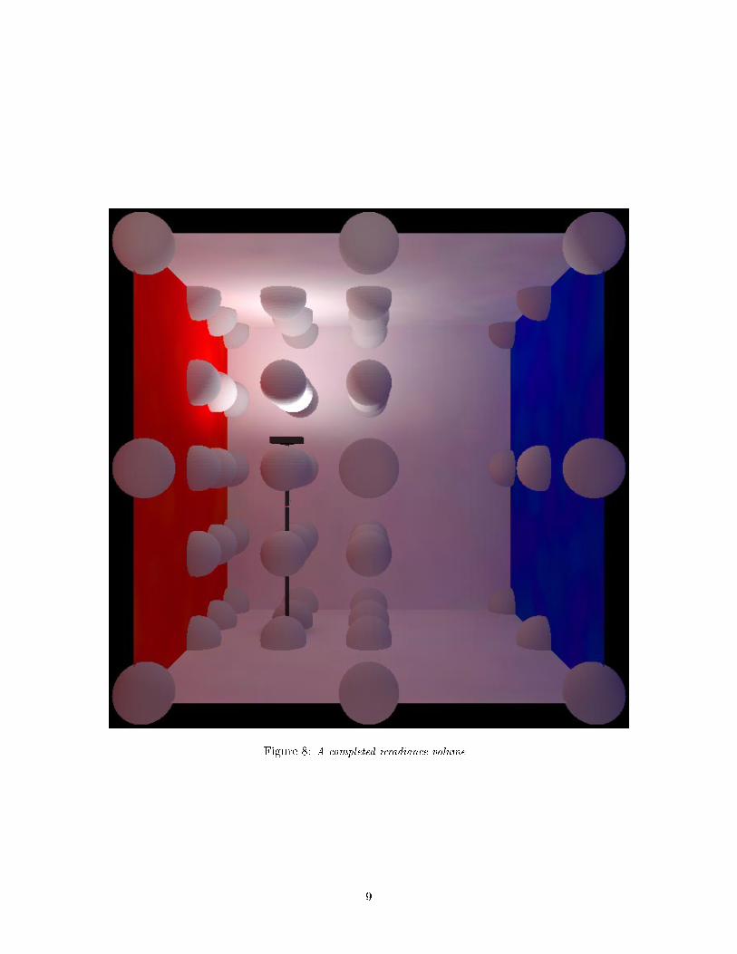
Figure 8: A completed irradiance volume.

9

1. Calculate which cell in the first-level grid contains x.

2. If the cell contains a grid, calculate which cell in the second-level grid

contains x.

3. Find which data value in the cell's samples corresponds to !.

4. Given the position of x within the cell and the eight values from the surrounding

samples, interpolate to get the irradiance.

Finding which cell contains a point is a simple operation, since the bounding box of the volume isknown. Finding the data values corresponding to a direction, !, involves inverting the hemispherical mappingdescribed earlier. Every spatial sample is stored as a pair of two-dimensional arrays. Each array representsthe irradiance computed over a hemisphere, with each array element corresponding to a direction in (u; v)space (Figure 5). A simple check is �rst performed on ! to determine which hemisphere contains it. Then,an inverse mapping of the method used in Section 3.2.1 is used to �nd the which bin on the unit square thedirection lies in. After the eight values are obtained, trilinear interpolation is used to get the irradiance ata point x.

4 Applications

4.1 Rendering Dynamic Objects in Semi-Dynamic Environments

Our de�nition of a semi-dynamic environment is one in which most surfaces are stationary, and the fewdynamic objects are small relative to the scale of the environment. For example, positioning a piece offurniture in an architectural application would fall into this category. An irradiance volume is well suitedfor semi-dynamic environments and can be used to approximate the global-illumination of dynamic objects.Such a system starts with a preprocessing stage that builds an irradiance volume from the static objects,as described in Section 3. Once the volume is built, it is queried to acquire the illumination of non-staticsurfaces.

This section presents an example implementation of an interactive semi-dynamic system and discussesseveral issues related to using the irradiance volume method in this context. Our implementation builds anirradiance volume in a environment rendered from a radiosity solution and allows a user to move an object,illuminated from the volume, around the environment. The model used for this example, an o�ce scene,is pictured in Figure 9. The dynamic object positioned under user control is a grey polygonal model of arabbit.

Figures 10 and 11 each show a sequence of frames of the rabbit in motion. In Figure 10 the rabbit movesfrom an open area of the o�ce to a position under the desk, becoming darker as it enters the desk's shadow.Figure 11 shows color-bleeding e�ects as part of the rabbit takes on a yellow tinge as it approaches a divider.

4.1.1 Performance

Building the Volume

The irradiance volume used for the o�ce model consists of a 73 (343) sample �rst-level grid and 72 3� 3� 3second-level grids, equaling a total 2287 samples. Each sample has a directional resolution of 2� 172 (578)angular bins. The volume took approximately 24 minutes4 to compute after the initial radiosity computationand used about 18 megabytes of main memory for storage. Figure 12 shows the structure of the completedvolume.

4All timings in this section were made on a Hewlett Packard 9000-715/100 system with a PA-RISC 7100LC processor (100Mhz, 121 MIPS, SPECfp92 138.3).

10

Figure 9: A view of the o�ce model.

11

Figure 10: Rabbit moving under desk.

12

Figure 11: Rabbit moving by divider.

13

Figure 12: The top image shows the �rst-level volume grid, and the bottom image the entire bilevel grid.

14

Querying the Volume

Ignoring system factors such as memory paging, querying the volume is a near-constant time operation.Algorithmically, queries will di�er at most by a \�nd which cell contains a point" operation, if the levelof hierarchy of the queried cells are not the same (Section 3.3). Finding the correct cell is a relativelyinexpensive procedure, resulting in only a small time di�erence between �rst- and second-level queries.

Because queries to the volume are well-bounded5, the use of the volume is well suited to time-criticalapplications. In addition, the volume supports6 levels of detail (LOD's) for dynamic objects. While the useris moving an object, the system can draw the lower resolution LOD, and then draw the higher resolutionLOD when stationary. The addition of a scheduling algorithm [9], could enable truly time-critical rendering.

Interacting with the Application

In a semi-dynamic application implementation of the kind presented here, three main computational proce-dures account for the large majority of time needed to compute a display frame. The geometry of the staticobjects are displayed (in this case the o�ce), the volume is queried to obtain the illumination of the dynamicobject or objects (the rabbit), and the dynamic geometry is displayed.

The o�ce model contains 43946 polygons and the rabbit contains 1162 polygons with 601 shared vertices,resulting in 45108 displayed polygons and 601 volume queries per frame. Using high-end graphics hardware7,we were able to achieve near real-time interactive rates, averaging approximately 5.3 frames per second.

4.1.2 Comparison with a Full Global-Illumination Solution

Several comparisons were made between a rabbit illuminated from the volume and a rabbit rendered using astandard radiosity method. To obtain a global-illumination solution, the polygonal rabbit model was addedto the o�ce environment and rendered using radiosity. A visual comparison8 was then made on imagesacquired from the two methods (Figure 13). As shown in �gure 13, the volume method provides a believableapproximation to the analytical solution9.

4.1.3 Display Issues

Self-Occlusion of Dynamic Objects

Signi�cant inaccuracies can result in the shading of object from the volume if it has large areas of self-occlusion. As discussed in the previous section, for a given direction !, the volume approximates theirradiance based upon the gathered radiance over the entire hemisphere centered around !. When theirradiance is queried at a point on an object whose hemispherical \view" of the environment is partiallyblocked by the object itself, the approximation obtained from the volume becomes less accurate. Theamount of potential inaccuracy caused by self-occlusion depends on how much of the hemisphere above apoint on the object is subtended by the object itself.

5The lower bound on the time it takes to illuminate an object from the volume can be expressed as the number of queries

� time it takes to perform �rst-level query. Similarly, the upper bound can be described as number of queries � time it takes

to perform a second-level query.6Some rendering algorithms attempt to take advantage of object coherence between frames, and run into problems if the

object changes. The irradiance volume is meant to be used to completely re-shade an object every frame. This means thatdynamic objects can be deleted, added, or modi�ed freely.

7An Evans and Sutherland Freedom 3000 series with 14 display processors.8There is not a standard metric for quantifying visual di�erences between images because there is no accurate model of

human vision. Direct visual comparison is currently the most practical method to evaluate images.9Note that the polygonal facets comprising the rabbits shown in the �gure are much more apparent than in previous images.

In the previous �gures, smoother shading was obtained by averaging the normals at vertices shared by several polygons. Theradiosity method used to make a comparison did not have the capability to interpolate the illumination between polygons.Because of this, the rabbit from the volume was displayed faceted for comparison purposes. Note that the facets tend tomaximize visual error; if both rabbits were displayed with interpolated shading, any di�erences would likely be less noticeable.

15

Figure 13: The images on the left were produced using the volume, and the images on the right were obtained from aradiosity solution. The top row shows the rabbits partly under a desk, the middle row shows them by the wall paintings,and the bottom row shows them in the center of the o�ce.

16

Shadows

In our implementation, dynamic objects do not cast any shadows on the environment. Calculating shadowsfrom an object due to indirect illumination is a di�cult problem and except for very simple cases, cannotbe performed quickly enough for use in interactive applications. Several high-end graphic systems, such as aSilicon Graphics RealityEngine system, support direct illumination in hardware and can compute shadowsat real-time rates.

4.2 Rendering Objects with High Complexity

Rushmeier et al. [10] discuss the use of geometric simpli�cation to accelerate global-illumination renderingsof complex environments. In their method, clusters of surfaces are replaced with optically similar boxesbefore performing the global-illumination calculation. After the global-illumination solution is obtained, itis used in rendering the original geometry. The irradiance volume can be used in an analogous manner.After a global-illumination solution is obtained with simpli�ed objects, an irradiance volume is built10. Thesimpli�ed geometry is then replaced with the original complex surfaces, which are shaded using the volume.This has the advantage over Rushmeier's method by using fast queries from the volume rather than anexpensive gather operation requiring tens or hundreds of traced rays.

We replaced one of the at walls in the model with a polygonal model of a cinder block wall. An irradiancevolume was created from a global solution of the room with the at wall (Figure 9). After the volume wasbuilt, each polygon of the cinder block wall was read into memory one at a time and rendered from thevolume. The wall consists of approximately 612,000 polygons; not counting disk-access time, it took about31 seconds to shade the polygons, entailing approximately 19,000 volume queries per second. Figure 14shows a view of of the wall.

Rendering Procedural Models

Many rendering algorithms produce complex procedural models while executing. The best known example isthe software developed by Pixar [11]. In Pixar's software, geometric primitives are processed independentlywithout reference to others, allowing the rendering of large scenes containing numerous highly-detailedcomplex objects. During rendering, each surface is composed with optional surface maps11, and diced into\micropolygons" which are then shaded and scan-converted. Because each primitive is rendered separately,only local illumination techniques are used to shade the micropolygons.

An irradiance volume could be used to approximate the global illumination on each micropolygon asit is created. This method would require an initial rough rendering of a scene using a global-illuminationalgorithm to get the approximate light ow in the environment. An irradiance volume would then be builtfrom this rough rendering and used to shade the micropolygons created during the �nal rendering.

5 Future Applications

5.1 Illuminating objects in picture-based environments

Picture-based methods use sets of pictures of an environment, either rendered or taken through photographicmeans, to compose a scene. Currently, picture-based methods are only used to render static environments.However, Chen [5] notes that interactive rendered objects can be composited onto a reconstructed view usinglayering, alpha-blending, or z-bu�er12 techniques. As these methods become more popular, picture-basedapplications containing non-static objects will likely increase in number.

Irradiance volume samples are taken at the same locations, or \nodes", as the radiance samples usedto form the picture-based environment. Actual views of an environment only exist at these nodes; views

10Note that the volume need not encompass the entire environment, but could be built only around a region of interest.11Such as texture, bump, and displacement maps.12If the pictures composing an environment are obtained through rendering, depth information can be recorded for each pixel.

This is, of course, impractical for photographically captured images.

17

Figure 14: A polygonal model of a cinderblock wall, illuminated from the volume.

at locations other than these nodes are either interpolated from the nodes or are ignored13, depending onthe application. If an application does support interpolation between nodes, additional volume samplescan be constructed between nodes from an interpolated image panorama. However, using this process onlymakes sense if the interpolated panoramas result in volume samples that provide better accuracy than simplylinearly interpolating between volume samples at the nodes (Figure 15).

The method used to acquire the radiance, L(x; !), is application-dependent, depending on such factors asthe way the image data is stored and the shape of the panorama at a node14. Once the radiance is sampled,the irradiance is computed using the method described in Section 3.2.3. Querying the irradiance from thevolume remains the same.

5.2 Illuminating Non-Di�use Objects

The irradiance volume can be extended to simulate non-di�use e�ects by storing higher order moments thanirradiance [3]. This allows the simulation of such phenomena as Phong-like glossy re ections, as long as thespecularity is not too high15.

13Some applications constrain the position of the viewer to the node locations.14In order to get a true radiance distribution at a point, data must be gathered over the entire sphere of directions. In

practice, cylindrical panoramas are often used instead to avoid problems inherent to spheres, such as the distortion and di�cultyof stitching images together at the poles. When sampling radiance from a cylindrical panorama, a default value needs to beassigned to the samples that are taken in directions which point out the top or bottom of the cylinder.

15One of the main assumptions in the creation of the irradiance volume is that we can interpolate between samples toget a good approximation of the irradiance. As we move away from irradiance towards increasingly specular functions, thisassumption becomes less valid.

18

OO

P0

P1

(b)

V V V V V0 01 1

P P P0 1

2

2

(a)

Figure 15: P0 and P1 represent panoramic views samples. P2 is a sample view interpolated from P0 and P1. V0, V1,and V2 are irradiance volume samples computed from their respective panoramas. In (a), the illumination of object Ois linearly interpolated from V0 and V1. In (b), the illumination is linearly interpolated from V0 and V2. If adding V2increases the accuracy of the illumination of O, the (application-dependent) node interpolation method can be used tocalculate volume samples at non-node locations.

To build a volume with higher-order moments, we use the following formula16 instead of Equation 4:

Hn(!) �

�n+ 1

2

�4�

N

NXi=1

L(!i)max(0; !i � !)n; (5)

where n is the order of the moment. Note that if n = 1, the above equation is equivalent to Equation 4, theformula we use to compute irradiance.

As discussed in Section 3.2.3, the irradiance in a particular direction ! is a cosine-weighted average ofradiance samples on the hemisphere oriented around !. As n increases, it has the e�ect of weighting theintegration of the radiance further towards !.

When a higher-moment volume is used in an application, changes must be made to the volume queryfunction. Since we are no longer storing and using irradiance to shade objects, the illumination on a surfaceis no longer view-independent. Queries to the volume must take into account the position of the viewer.Instead of querying in the direction of the normal of the surface, the view vector is mirrored about thenormal to obtain the query vector in the direction of specular re ection.

As n increases, the frequency of the illumination function also rises. As it becomes more specular,higher directional and spatial sampling rates are needed to maintain a good approximation. In addition,interpolated shading across a surface (such as Gouraud shading) becomes less accurate. Objects which querythe volume to get the illumination at their vertices may need to be composed of �ner meshes for good results.

6 Conclusion

This paper presented an exploratory study on the feasibility and e�ectiveness of sampling and storing irra-diance in a spatial volume. Constructing a volumetric approximation of the irradiance throughout a spaceenabled the approximate irradiance at any point and direction within that space to be quickly queried. Thisallowed the reconstruction of believable approximations to the illumination in situations which overwhelmtraditional global illumination algorithms, such as semi-dynamic environments.

Acknowledgments

Jim Arvo supplied several ideas, including using higher moments than irradiance. Dani Lischinski providedcode used to make radiosity solutions. Ian Ashdown provided pointers to valuable references. The rabbitmodels are courtesy of Stanford University and the University of Washington. This work was supported bythe NSF Science and Technology Center for Computer Graphics and Scienti�c Visualization (ASC-8920219).Much of the work of this project was conducted on workstations generously donated by the Hewlett-PackardCorporation.

16The notation Hn is used here to indicate the nth moment of H.

19

References

[1] C. Cuttle. Lighting patterns and the ow of light. Lighting Research and Technology, 18(6), 1971.

[2] Gregory J. Ward, Francis M. Rubinstein, and Robert D. Clear. A ray tracing solution for di�useinterre ection. In John Dill, editor, Computer Graphics (SIGGRAPH '88 Proceedings), volume 22,pages 85{92, August 1988.

[3] James Arvo. Analytic Methods for Simulated Light Transport. PhD thesis, Yale University, December1995. This text is available from http://csvax.cs.caltech.edu/ arvo/papers.html.

[4] Daniel Lischinski, Filippo Tampieri, and Donald P. Greenberg. Combining hierarchical radiosity anddiscontinuity meshing. In Computer Graphics Proceedings, Annual Conference Series, 1993, pages 199{208, 1993.

[5] Shenchang Eric Chen. Quicktime VR - an image-based approach to virtual environment navigation. InComputer Graphics (SIGGRAPH '95 Proceedings), Computer Graphics Proceedings, Annual ConferenceSeries, pages 29{38, July 1995. ACM Siggraph '95 Conference Proceedings.

[6] Christopher Patmore. Illumination of dense foliage models. In Michael F. Cohen, Claude Puech, andFrancois Sillion, editors, Fourth Eurographics Workshop on Rendering, pages 63{72. Eurographics, June1993. held in Paris, France, 14{16 June 1993.

[7] Ned Greene. E�cient approximation of skylight using depth projections. Photorealistic Volume Modelingand Rendering Techniques, 1993. ACM Siggraph '91 Course Notes 27.

[8] Peter Shirley and Kenneth Chiu. Notes on adaptive quadrature on the hemisphere. Technical Re-port 411, Department of Computer Science, Indiana University, July 1994. This text is availablefrom http://www.cs.utah.edu/ shirley/papers.html.

[9] Thomas A. Funkhouser and Carlo H. Sequin. Adaptive display algorithm for interactive frame ratesduring visualization of complex virtual environments. Computer Graphics, pages 247{254, August 1993.ACM Siggraph '93 Conference Proceedings.

[10] Holly Rushmeier, Charles Patterson, and Aravindan Veerasamy. Geometric simpli�cation for indirectillumination calculations. In Proceedings of Graphics Interface '93, pages 227{236, Toronto, Ontario,Canada, May 1993. Canadian Information Processing Society.

[11] Robert L. Cook, Loren Carpenter, and Edwin Catmull. The reyes image rendering archtecture. Com-puter Graphics, 21(4):95{102, July 1987. ACM Siggraph '87 Conference Proceedings.

20