THE BELL SYSTEM

TECHNICAL JOURNAL

volume xxxiv MARCH1955 number2

Copyright, 1955, American Telephone and Telegraph Company

Transport Properties of a Many-Valley

Semiconductor

By CONYERS HERRING

(Manuscript received December 16, 1954)

The simple model of a semiconductor, based on a single effective mass for the charge carriers and a spherical shape for the surfaces of constant energy, is now known to be inadequate for most of the semiconductors which have been extensively studied experimentally. However, some of these do corre- spond to what may be called the "many-valley" model, a model for which the band edge occurs at a number of equivalent points K(,) in wave number space, and for which the surfaces of constant energy are multiple ellipsoids, one centered on each of these points. This paper develops, for models of this type, the theory for: mobility (Section 2) and Us temperature dependence (Section 3); thermoelectric power (Section Jf); piezoresistance (Section 5); Hall effect (Sections 6 and 9); high-frequency dielectric constant (Section 7); and magnetoresistance (Sections 8 and 9). These phenomena are treated, for cases to which Maxwellian statistics apply, on the assumption that the scattering of the charge carriers is describable by a relaxation time which de- pends on energy only, but is otherwise unrestricted. This assumption can be shown to be justified in a large class of cases, although for some cases it fails, notably when ionized impurity scattering predominates and at the same time the effective mass is very anisotropic. Special attention is given to the role of inter-valley lattice scattering, i.e., to processes whereby a charge carrier is scattered from the neighborhood of one of the band edge points

237

238 THE BELL SYSTEM TECHNICAL JOURNAL, MARCH 1955

K(,) to the neighborhood of a different one. Numerical calculations are pre- sented which show the effects of such processes on the magnitudes and tem- perature variations of the effects listed above.

1. THE MANY-VALLEY MODEL

Most of the literature of semiconductor theory has been based on what we shall call the simple model. This model is based on the assumption that the minimum energy in the conduction band, or the maximum energy in the valence band, is possessed by only one quantum state of either spin. This state has the form of a Bloch wave with wave number K = 0.* States with energies near the band edge value therefore have small K values, and, since their energies £(K) must vary continuously with K in this region, e(K) for small K must be a quadratic form in Kz , Ky , K,. If the crystal structure is cubic, e(K) a K1, and the sur- faces of constant energy are spheres in K-space.

It has long been known that other models are possible, and indeed likely in many cases. In recent years it has become clear that the simple model does not apply to any of the four cases corresponding to n- and p- type germanium and silicon. The evidence for this includes magneto- resistance1, 2'3 and piezoresistance4 effects, cyclotron resonances,5 and many other phenomena. Now the possible alternatives to the simple model are the various models for which there is more than one state, apart from spin degeneracy, with the band edge energy. These models fall into two general categories.

(A) Models for which the band edge energy occurs for several wave number vectors K*0, but for which there is only one state of each spin having this energy and a given K(0. For a conduction band model of this sort the energy e, considered as a function of K, has a number of minima or "valleys", hence we shall call these "many-valley" or "simple

* For the convenience of the reader the notations defined in the text are re- capitulated on page 288.

1 I. Estermann and A. Foner, Phys. Rev., 79, p. 365, 1950; G. L. Pearson and H. Suhl, Phys. Rev., 83, p. 768, 1951; and G. L. Pearson and C. Herring, Physica, to appear. 2 W. Shockley, Phys. Rev., 78, p. 173, 1950, and unpublished work.

3 S. Meiboom and B. Abeles, Phys. Rev., 93, p. 1121, 1954; B. Abeles and S. Meiboom, Phys. Rev., 95, p. 31, 1954; and M. Shibuya, J. Phys. Soc., Japan, 9, p. 134, 1954 and Phys. Rev., 95, 1385, 1954. 4 C. S. Smith, Phys. Rev., 94, p. 42, 1954.

8 G. Dresselhaus, A. F. Kip, and C. Kittel, Phys. Rev., 92, p. 827, 1953; B, Lax, H. J. Zsiger, R. N. Dexter, and E. S. Rosenblum, Phys. Rev., 93, p. 1418, 1954; R. N. Dexter, H. J. Zeiger, and B. Lax, Phys. Rev., 95, p. 557, 1954; R. N. Dexter, B. Lax, A. F. Kip, and G. Dresselhaus, Phys. Rev., 96, p. 222, 1954; and R. N. Dexter and B. Lax, Phys. Rev., 96, p. 223, 1954.

TRANSPORT PROPERTIES OF A MANY-VALLEY SEMICONDUCTOR 230

many-valley" models. For a valence band the situation is similar, but inverted.

(B) Models for which, apart from spin degeneracy, there are two or more states with the band edge energy and the same wave number vector. These we shall call ''degenerate" models. We may subdivide them further into "degenerate single-valley" and "degenerate many-valley" cases according to whether the band edge energy occurs for only one wave vector, or for several.

This paper is concerned with the transport properties of the simple many-valley models defined under (A). These models are much simpler to handle than the degenerate types, for reasons which are illustrated in Fig. 1. This illustration shows schematically the form in wave number space of the surfaces of constant energy, near the band edge energy, for four models. For the simple model, shown in (a), the locus of a given energy is, as already stated, a sphere. For a simple many-valley model, shown in (b), the locus is a set of ellipsoids centered about the band edge points K1". The ellipsoidal shape is required by the facts that energy must depend continuously and different iably on K and have an extremum at each K'0. For a degenerate model, however, the dependence of energy on the components of K is singular at the band edge point," in that unique second derivatives do not exist: energy varies quadrati- cally with K in any given direction from this point, but the coefficients going with different directions are determined by a secular equation. The result is that the contours of constant energy may look as shown in Fig. 1 (c) (degenerate single-valley case). Degenerate many-valley cases are of course similar, but with the surfaces multiplied, as in Fig. 1(d). Such situations are obviously harder to handle mathematically than those of Fig. 1(b).

Besides the irregularity of the energy surfaces, there is another dif- ference between these two types of cases which greatly complicates theo- retical work with degenerate models. This is that in most cases the energies of the two or more states going with a given band-edge K will be split by spin orbit coupling. If this splitting is «.kT it can usually be ignored, and if it is »/iT it may effectively convert the degenerate model into a simple or simple many-valley model. Unfortunately, it usually happens that neither of these extremes applies, and for such inter- mediate cases not only do we have to deal with energy surfaces like those of Fig. 1 (a), but, much worse, the variation of energy with K is not a simple quadratic dependence even in a fixed direction from the band edge point.

In view of all these complications of the degenerate models, it is for-

240 THE BELL SYSTEM TECHNICAL JOURNAL, MARCH 1955

tunate that the simple many-valley case does seem to occur for n-type silicon and n-type germanium. One of the best ways of finding out whether it occurs for any given semiconductor is to compare observa- tions on this material with theoretical predictions for the various possible models of the simple many-valley type. We proceed now to derive these predictions, assuming for simphcity that the charge carriers have Maxwellian statistics and an effective relaxation time dependent only on energy. We shall take up the simplest properties first, the more com- plicated ones later. Sections 2 to 5 will consider perturbation of the distribution function of the carriers by a static electric field, Section 6

-KX

(

Ky

)

( )

Kx

(a) SIMPLE

(b) SIMPLE MANY-VALLEY

(C) DEGENERATE

(d) DEGENERATE MANY-VALLEY

Fig. 1 — Different types of band structure for a semiconductor, illustrated by the forms of the surfaces of constant energy in wave number space. The band edge points are represented by heavy dots.

TRANSPORT PROPERTIES OF A MANY-VALLEY SEMICONDUCTOR 241

the Hall effect, Section 7 the perturbation by an oscillating electric field, Section 8 magnetoresistance, and Section 9 effects at high mag- netic fields.

In presenting this material our primary objective will be to provide a coherent treatment of all the effects in language as simple and physical as possible. Thus, for example, the Hall and magnetoresistance effects will be discussed ab initio, although many of the details presented here have been derived and published independently by several workers.2'3

Nor is the theory of this paper the ultimate in refinement: at cost of a little more mathematical complication, the assumption of a relaxation time dependent only on energy can be dispensed with, and anisotropy in the scattering processes acting on the carriers can be taken into ac- count.6 However, the present simpler treatment illustrates most of the physical principles involved in the various phenomena, and turns out to be quantitatively adequate in a large class of cases.

2. CONDUCTIVITY

In this section we shall solve the Boltzmann equation for the effect of a constant electric field E on the motion of charge carriers in a simple many-valley band. Maxwellian statistics will be assumed. Thus if AP = h (K — K0') measures the deviation in crystal momentum space from one of the band edge points K(,>, then for E = 0 the proba- bility of occupation of the state described by AP (by an electron or hole, depending on the sign of the carriers) is

/(0) = exp ep — tb APi _ AP, AP,2-

(1)

where eF is the Fermi level, et the band edge energy and mi*, in,*, m,* arc the effective masses in the three coordinate directions 1, 2, 3 which are principal axes for the energy surfaces of the valley in question. When E = ^ 0 the distribution function/is determined by the competi- tion between the perturbing effect of E and the restoring effect of scatter- ing processes which try to restore the form (1). To make the problem tractable we shall assume that the scattering processes which the charge carriers undergo are described by a relaxation time which is a function of energy e only. In other words, we shall assume that for any slight

6 C. Herring and E. Vogt, to be published.

242 THE BELL SYSTEM TECHNICAL JOURNAL, MARCH 1955

departure off from/(0) the time rate of change off due to collisions is

The legitimacy of this assumption is analyzed in Appendix A. It is shown there that the assumption should be rather accurately valid for all kinds of inter-valley scattering — defined as scattering from the neighborhood of one band edge point K0' to the neighborhood of another K0> — and for intra-valley lattice scattering due to optical modes or to neutral impurities, provided, in the latter case, that the temperature is low enough. For intra-valley lattice scattering due to acoustical modes the assumption r = rfe) is not necessarily valid, but the arguments of Ap- pendix A suggest tht it will often be a good approximation. For scatter- ing by ionized impurities, however, this assumption will usually be a poor approximation. There is a good prospect that in the near future the adequacy of this approximation for lattice scattering can be quanti- tatively estimated for some substances. If it should turn out to be in- adequate, the necessary generalization of the calculations of this paper can probably be made without great effort.

With the assumptions just stated in (1) and (2), the Boltzmann equa- tion for a steady state in the presence of a field E takes the form

where the upper sign is for electrons in a conduction band, the lower for holes in a filled band. If, as is customary, we set

Having obtained the solution of the Boltzmann equation in the form (4), (5), we shall now evaluate the electron current density j from it. If /(0) is Maxwellian,

(2)

(3)

f = /(0) + E-f(1) + OiE2),

(3) gives, just as in the simple theory,

f(1) = ±erVp/<0)

(4)

(5)

V/'Ae AT f (6)

where v is the group velocity and Ae = | e — o, | is the distance from the band edge. The contribution of carriers in the ith valley to the current

TRANSPORT PROPERTIES OF A MANY-VALLEY SEMICONDUCTOR 243

density is then

r'= E (± ^vtAP'^/tAP1") ipU).s

= if T. /"VAOE-W (7) kl 4p(«),s

where the summations are over all AP1" occurring in the ?"th valley in unit volume of material, and over both states of spin.

The expression (7) states that any single valley i possesses an aniso- tropic conductivity tensor Oafl0', or an anisotropic mobility tensor ga/?0*, i.e.,

ia(0 - Z = Z {nU)ena0(i))E0 (8)

where

n - = E /<°, (9) .to _ ApO'Ls

is the number of carriers in valley i per unit volume. If we choose the x, y, and z axes to be along the principal axes of the ellipsoidal energy surfaces of valley i, (7) shows that Vad" and yag{" will be diagonal. Each diagonal element gu0' will involve a Maxwellian average of V\T(Ae). Now the equipartition principle leads us to expect that the average, over an energy shell Ae to Ae + dAe in AP-space, of the kinetic energy asso- ciated with the ^-component of velocity should be the same as that as- sociated with the y- or ^-component. This is easily demonstrated ex- plicitly (Appendix B). Thus, if vh*, m*, vi * are the effective masses in the three principal directions,

'<2 = ]4 mi*v{ = lo m3*V3 (10)

Therefore (7) and (8) give, in our system of axes,

(.•) e <A€r> , , g«a - —5 . (U) ma* <Ae>

ga(J(<) = 0 (a ^ /3) (12)

where the angular brackets denote Maxwellian averages:

<Aer> - ZAer/(0)/Z/(0),etc. (13)

The denominator of (11), <Ae>, of course equals % /."7' by equipartition.

244 THE BELL SYSTEM TECHNICAL JOURNAL, MARCH 1955

The formula (11), it will be noted, is the same as that of the simple theory7 with m* replaced by ma*.

The overall conductivity tensor due to the carriers in all the valleys is of course ail(l the overall mobility tensor is the average of /Xa/3(,) over the different valleys. For a cubic crystal the mobility is the same in all directions, so we have

M =/iXX = HJl Maa = Maa<,>

1 " (14) e <AeT>

miI) <A€>

where Nv is the number of valleys and ma) is an average inertial mass defined by

—77T = r —* + —* + —- mil) [jn* m-* m-.( (15)

This mass, as we shall see in Section 7, is the one most directly meas- ured by the Benedict-Shockley experiment on high-frequency dielectric constant.

3. TEMPERATURE VARIATION OF LATTICE MOBILITY

The r occurring in the mobility expression (14) differs from the r of the simple model in that it contains the effect of inter-valley scattering in addition to intra-valley and impurity scattering. Inter- and intra- valley scattering differ in that most of the phonons emitted or absorbed in intra-valley scattering have energies « the energies of the charge carriers, while those involved in inter-valley scattering usually do not. If K(,> and K0) are two different band edge points, scattering of a carrier from valley i to valley./ must involve emission or absorption of a phonon of wave number close to ±q,j , where = K(,) - K(y). If q.y has a mag- nitude of the order of the radius of the Brillouin zone, as is likely in most cases, the energy ftco.-y of this phonon will be a major fraction of of kQ, where 0 is the Debye temperature. This is usually ^kT in the extrinsic range. One must therefore use the Planck, rather than the Rayleigh-Jeans, distribution function for these phonons. At very low temperatures, inter-valley scattering is negligible: absorption of an ij phonon is rare because few such phonons are present; emission is com-

7 See, for example, W. Shockley, Electrons and Holes in Semiconductors, (Van Nostrand 1951) p. 276.

TRANSPORT PROPERTIES OF A MANY-VALLEY SEMICONDUCTOR 245

parably rare because few carriers have energy enough to create such a phonon. With rising temperature inter-valley scattering becomes more important. This causes r (hence n) to decrease more rapidly with increasing T than it would if there were no inter-valley scattering. In this section we shall develop this idea quantitatively.

The matrix element for scattering of a carrier from some state in valley i to another state in valley;, by absorption or emission of a phonon hu, has the form common to all one-phonon scattering processes8

^y = ^\n4j5.7for(absorPtio11 (16) (TV + 1) J (emission K J

where N is the number of phonons of the given type present in the initial state and where Z),;- is independent of the occupation of the phonon states. For inter-valley scattering is practically independent of the locations of the initial and final states in their respective valleys. In general, of course, D.y will be different for the different branches of the vibrational spectrum. The transition probability from a state of energy e in valley i to a state in valley; of energy e' = e + hu (absorp- tion) or e - hco (emission) is proportional to | Mij |2 times the density of states at energy e' in the ;th valley, provided the variation of hco with position in the valley is negligible, as is the case for most transitions. Since the number of states between e' and e' -j- de' is proportional to Ae,1/2 dAe', where Ae' is the distance from the band edge, this transition probability has the form

absorption: Wa ^ (17) exp (hu/kT) — 1 u';

• • ttt- (^e — hu)112 emission: We cc for Ae > hco

1 — exp (— hco/kT) (-jg)

0 for Ae < hco

Since either of the processes (17) and (18) randomizes the initial velocity of the charge carriers, and since in this paper we are assuming the existence of an effective relaxation time r.-^e) for randomization of velocity by the intra-valley scattering of acoustic modes, the total relaxation time for lattice scattering is given by

11 ' - := h S [Wa(ij, a) + We(ij,a)] (19) T T U j,a

where a labels the branches of the vibrational spectrum and ira and We 8 See, for example, Reference 7, p. 520.

240 THE BELL SYSTEM TECHNICAL JOURNAL, MARCH 1955

TOTAL

INTER VALLEY

INTRA— VALLEY

INTER- VALLEY / —

t Af

1-^(^(12,1) r0 01(12,2)

j iLwds^) \ho)(l3,2)

hoi (13,1)

hcu(i2,i); i ho;(12,2) /

ho; (12,3

-hoidSjS), . —ho)(13,2) I

-ho)(l3,l) —h O) (12,3)

Fig. 2 — Contributions to the reciprocal relaxation time of a charge carrier, due to inter-valley and intra-valley lattice scattering. The dot-dash curves are the inter-valley scattering contributions a) for emission of a phonon, the dashed curves are the corresponding quantities 11 a(ij, «) for absorption of a phonon. There are many transitions from valley 1 to different ones of the other valleys, due to different branches a of the phonon spectrum.

are given for each type of transition by (17) and (18) respectively, with hu = hu(ij, a). The prime on the summation means that when a is an acoustic branch, the term j = i is to be omitted. However, since (17) and (18) apply to intra-valley scattering by modes of the optical branches, such scattering is included in (19) as the terms with j = i. Fig. 2(a) shows the various contributions to l/r as functions of the initial energy • 1/2 " Ae of the carrier being scattered: l/r,-,- is proportional to Ae , as m the simple theory (this corresponds to a mean free path independent of energy for any given direction of motion), and each of the other terms is proportional to some (Ae ± liu)x

We shall try to estimate the order of magnitude of the steepness of

TRANSPORT PROPERTIES OF A MAXY-VALLEY SEMICONDUCTOR 247

the parabolas describing the various inter-valley terms, relative to that ol the intra-valley term For the low-frequency acoustic modes involved in intra-valley scattering the factor Da in the matrix element (16) is proportional to q/(hu)v'2, and since u cc q and N kT/hu » 1 for such modes | M/j \2 ^ T and is independent of q. The g's involved in inter-valley scattering will usually be too large to satisfy kT/hu » 1, at least in the extrinsic ranges of Ge and Si, but we may hope to estimate a plausible order of magnitude for their TFa's and IFe's by assuming their Z)(/s to be a q/hw with a factor of proportionality of the same order as for intra-valley scattering. With this assumption the steepness of a typical iij) parabola corresponding to phonon emission (PFe) should be of the same order as the steepness of the intra-valley parabola when kT ^ hw(ij), while lor kT < hw(ij) the We(ij) parabola should become nearly independent of T, as contrasted with l/r.-^e) a T. The parabolas corresponding to phonon absorption are of course always less steep, the ratio of the steepness of Wa(ij) to that of We(ij) being

Wal(At + /to)"2 1 - exp (- hu/kT) = exp (- hu/kT) (20) TTV(Ae - /to) 1/2 — exp (hw/kT) — 1

TOTAL /

/ INTER-VALLEY / EMISSION

/ / / / / / / /

/

f INTER-VALLEY S / ABSORPTION

^ INTRA-VALLEY

l / / / 1

Af

Fig. 3 — Same as Fig. 2, but for the simplified model of Equation (24), on which the numerical calculations of Figs. 4, 5, 8, 9 and 10 are based.

248 THE BELL SYSTEM TECHNICAL JOURNAL, MARCH 1955

Because of the large number of terms Wa,e{ij, a) in (19) or Fig. 2, each with an at present unknown amplitude and critical frequency, it would be pointless to undertake calculations taking individual account of all the possible types of transitions. However, it is reasonable to hope that the behavior of the inter-valley terms can be roughly approximated by a model which considers absorption and emission of just a single type of inter-valley phonon. This model is illustrated in Fig. 3. It contains three adjustable parameters Wi, Wi, and hu, defined by

/AeY'2 AA i/T" ~ Wi \W

Wa =

We =

Ae W2 ^ + 1

1/2

exp (hu/kT) — 1

1 — exp (— Jua/kT) or 0

(21)

(22)

(23)

Equation (19) becomes

WlT =

Aey'YMV^ hid) \h(d) Wi

Ae ^ +1

1/2 Ae hid

1/2 or 0

_exp (hid/kT) — 1 1 — exp (— hid/kT).

(24)

Thus Wit is a function of the two variables Ae/hid and kT/hid, and the single parameter wz/wi . The behavior of the mobility as a function if kT/hid therefore depends, apart from the constant scale factor Wi, only on W2/W1 .

Fig. 4 shows the results of some calculations of this mobility-tempera- ture relation, made by numerical evaluation of (24) and (14). It is evident that with reasonable values of wz/wi, the negative exponent describing the temperature variation of the mobility can be increased to a value considerably above the % of the simple theory, over a considerable range of temperature. This is often what is needed to explain the ob- served mobility behavior. In Sections 4, 6, and 8 we shall see the extent to which this mobility exponent is correlated with, respectively, the electronic part of the thermoelectric power, the ratio of Hall to drift mobility, and the magnitude of the magnetoresistance.

TIUNSPOET PROPERTIES OF A MANY-VALLEY SEMICONDUCTOR 249

3 V77 e (uo =

6.C 2,3

6.0

4.0

2.9 2.0

2.05 1 .0 0.6

VALUES OF -d LOG LL 0,6

2.5 d LOG T 0.4

\ 0.2

VALUES W2

°F I W, V y.

0.0 8 0.06

0.5 1.55 0.04 1.0

0.02 1.6

2,0 4.0

0.2 0.4 0.6 .0 KT no;

6 8 10

Fig. 4 — Mobility-temperature curves for pure lattice scattering, as obtained from the simplified expression (24) for the relaxation time. The quantities wi and wi measure the strength of the coupling of the carriers to intra- and inter- valley modes, respectively; a> is the frequency of the inter-valley mode. The curves have been drawn so as to smooth out irregularities in the computed points.

250 THE BELL SYSTEM TECHNICAL JOURNAL, MARCH 1955

4. THERMOELECTRIC POWER

The thermoelectric power of a semiconductor is a little different from the other effects discussed in this paper, in that it involves not only the response of the distribution function of the charge carriers to a per- turbing temperature gradient or electric field, but also the alteration of the distribution function of the phonon system.9, 10 The duality mani- fests itself in the apperaance of two contributions to the thermoelectric power Q: the measured Q is the sum of an electronic part Qc, representing the emf necessary to counteract the tendency of charge carriers to diffuse from hot regions to cold, and a phonon part Qv , representing the emf nec- essary to counteract the drag exerted on the carriers by the phonons which flow down the temperature gradient in thermal conduction. As the present paper is devoted to effects having to do with the response of the electronic distribution function to various influences, and as all aspects of the theory of thermoelectric power have been discussed else- where,10 we shall limit the present section to a discussion only of the electronic part Qe, which, fortunately, predominates greatly over Qp

at high temperatures. The expression for Qe is most simply derived by making use of the Kel-

vin relation Qe = TT/T between Qe and the electronic contribution IT to the Peltier coefficient, which represents the energy flux, relative to the Fermi level, which accompanies the transport of unit charge in an isothermal conduction process. For an intrinsic semiconductor with low carrier concentration

eTQc = cllc = tf — eb — Aer (25)

where as before eF is the Fermi level, eb the band edge energy, and where Aer is the average energy of the transported electrons relative to the band edge, a quantity >0 for n-type material, <0 for p-type, and of the order of magnitude of kT. Now | eF - o, | can be expressed in terms of the carrier concentration n and the effective masses. For a many-valley model the number of carriers n'0 in each valley is easily shown to be the same as for a simple model semiconductor with the same | tp — tn \ and with an effective mass equal to the geometric mean of the principal masses mi*, mf, m-f of the valley. This is because the density of states in energy is proportional to the volume of K-space inside an energy sur- face, a quantity which for a spherical surface goes as the cube of the radius, and for an ellipsoidal one as the product of the principal semi-

'JII. P. R. Frederikse, Phys. Rev., 92, p. 248, 1953. 10 C. Herring, Phys. Rov., 96, p. 1163, 1954.

TKANSPORT PROPERTIES OF A MANY-VALLEY SEMICONDUCTOR 251

axes. The total carrier concentration is therefore

n = Nyn'0 = 2(2'^r)"2 (mi*mi*m3*y'sNr exp

where ArK is the number of valleys. The final expression for Qe obtained by expressing ; e? — t(, | in terms of n and inserting in (25) is

Qe = T

1.2 ^n — 70 X 10 15

/W Vh* \ m m

80.2 fn ^ /"n Ny + y2 In \ m m m /

(26)

+ %taT + w/deg.

where n is in cm-3 and the upper sign is for n-type material, the lower for p-type.

If a relaxation time exists, dependent only on energy, the distribution function for isothermal conduction has the form/(0) -f- E-f(1) worked out in Section 2, and we have, for a cubic crystal,

_ /AeV-f(1) dP = <Ae-T>

jv-f(1) dP <Aer>

I I i-iC v X LLAT \LAt I' J' I — <(1) — s A . ^

by (5), (0) and (10), where as before the angular brackets denote Maxwel- lian averages as defined by (13).

It is important to know the value of (27) as accurately as possible, in the temperature range where Qe is measurable, since if (27) is known the measured Qe can be used with (26) to give information on the effective masses. For pure intra-valley scattering, (27) has the value 2kT. Im- purity scattering increases Aer by causing the current to be carried more by fast carriers and less by slow; inter-valley scattering has the reverse effect. It is worth while to try to correlate the effect of inter-valley scattering on Ae^ with its effects on two measurable properties, namely, the temperature variation of mobility (Section 3) and the ratio of Hall to drift mobility (Section 0). Accordingly, calculations of | Aer | have been made using the expression (24) (model of Fig. 3) for the relaxation time. The results are shown in Fig. 5, which shows | Aer \/kT as a func- tion of kT/hw.

5. PIEZORESISTANCE

As we have just seen in Section 2, the quantum states in any small region of wave number space make a contribution to the conductivity

252 THE BELL SYSTEM TECHNICAL JOURNAL, MARCH 1955

2.0

1.9

1.B A£l kT

1.7

1.6

'"o.l 0.2 0.3 0.4 0.6 0.8 1.0 2 3 4 5 kT tiu;

Fig. 5 — Values of the thermoelectric transport ratio | \/kT defined by (27), for the simplified lattice scattering law (24). The ratio wi/w\ measures the strength of the coupling of the carriers to inter-valley modes in terms of that for intra- valley scattering; oj is the frequency of the inter-valley modes. The curves have been drawn to smooth out irregularities (severe for kT/hu = I to 2) in the cal- culated points.

which depends on (i) the degree to which these states are populated in the equilibrium distribution/(0), (ii) their group velocity, and (iii) their relaxa- tion time, or more generally, the transition probabilities for scattering from these states to others. When the crystal is strained, any or all of these factors may change, and the resulting change in the sum of all the local contributions to the conductivity constitutes the piezoresistance effect recently discovered by Smith.4 Although there are a number of processes which can contribute to the three factors (i) to (iii) just enumerated, it can be argued plausibly that for a simple many-valley model the principal effects are usually those due to a single process, namely, the strain-induced shifts of the energies ct- of the band edge points K(,). We shall consider (i) to (iii) in turn:

(i) The change in the population/^(K'0 + AK) depends on the shift of the energy e{K{i) + AK), and because.of the smallness of AK this is practically the same as the shift 8eU) of e(K(,)). In a shearing strain some of the 5e(0 will be positive, some negative, and so some of the valleys will have their populations decreased, some increased, the fractional change in each case being 8el)/kT. Now it is evident from the second equation of (7) that the contribution of a single valley to the conductivity is aniso- tropic. If all valleys are populated equally, as we assumed in Section 1, the total conductivity will be isotropic. But if strain causes different valleys to have different populations, the overall conductivity will have

w2 V^=0-5 :

\ 1.0

N V. 2^9. 4.0

TRANSPORT PROPERTIES OF A MANY-VALLEY SEMICONDUCTOR 253

an anisotropy like that of the more populous valleys. If the ratio of 6e(,)

to the shear strain amplitude is of the order of magnitude of the known ratio of 5e0 to strain for isotropic compression, viz., a few volts, the frac- tional change of/"" per unit strain will be of the order of hundreds. Since the observed fractional change in resistance per unit shear strain is of the order of 10" in the more favorable orientations,4 the change in/(0) is of the right order of magnitude to contribute a major part of the effect.

For an isotropic compression or dilation there exists the possibility, not present for shearing strains, that the total carrier concentration may be changed in first order. A large effect of this sort, again of the order of the btx)/kT, will occur for a specimen in or near the intrinsic range, be- cause of the change of energy gap €G with strain. This effect rapidly becomes negligible, however, as the specimen is made extrinsic. For ex- ample, if unit volume of an n-type specimen has an excess nD of donors over acceptors, all ionized, the hole and electron concentrations n/, , ne, obey

where n,(T) is the value of nc = iih in intrinsic material. Thus if nn » m

and since dne/dtu = dnu/dta, the energy gap effect is negligible if nD

exceeds iii by a large factor, even though the change in n,- with strain may be sizable. For extrinsic specimens with incomplete ionization of impurity centers, there may of course be an effect of compression on total carrier concentration due to change in the ionization energy of the centers; however, if this ionization energy is «eG this effect will be of a smaller order of magnitude than the 5e("/kT.

(ii) It is easy to show that the fractional change in group velocity per unit strain must be much smaller than the bel)/kT just discussed, hence too small to contribute in a major way to the piezoresistance ef- fect. For we expect the change bw in the group velocity at K(,) + AK to have an order of magnitude given by

bv ~ [5e(K(*) + AK) - b€{i)yhMv ~ (AK/K{i))2(be(i)/hAK)

since the quantity in square brackets must vary as AK2. Since

ne = no -f iih , nenh = w,"

(28)

[e(K(l) + AK) - t(i)]/hAK = Ae/hAK

we have

bv/v ~ (A7v/iv<,))2(5e(,)/Ae) (29)

254 THE BELL SYSTEM TECHNICAL JOURNAL, MARCH 1955

Since a typical charge carrier has Ae ~ kT, (29) is smaller than the ratio discussed in the preceding paragraph by the factor (Aiv/Ku))2. It is thus plausible to neglect strain-induced changes in group velocity, or equiva- lently, in the effective masses.

(iii) Consider the transition probability from a state K to the group of states lying in a small element of volume in K-space, centered on a point K' at which the proper energy conservation law for the transition K —* K' is satisfied. This probability, like all quantum-mechanical transition probabilities, can be expressed as the product of the square of a matrix element M(K, K') by the number of states per unit energy in the given element of volume. We have to consider the effect of strain on each of these factors.

The matrix element M(K, K') can be changed either by a change in the wave functions , or by a change in the physical processes determining the perturbation operator M, e.g., a change in the ampli- tudes of the thermal vibrations, or a change in the dielectric constant, which enters into scattering by charged impurities. Typical assumptions on the equation of state of a crystal suggest that the fractional change in the squared vibration amplitude, per unit strain, might be of the order of a few units, i.e., at least an order of magnitude less than the observed elastoresistance for the optimum orientations. The effect of the change in the wave functions is of similar magnitude: To effect a major change in M(K, K') one must make a major change in the wave func- tions. To do this probably usually requires a strain of amplitude 0.1 to 1. Therefore it is reasonable to expect that the fractional change in j M' \ per unit strain will be of the order of 10 or less, i.e., again an order of magnitude smaller than Se^/kT, or than the observed elastoresistance.

The effect of strain on the density-of-states factor, on the other hand, can be larger. For intra-valley scattering, where initial and final states are both near the same band edge point K0', the effect is of course very small, since initial and final states undergo very nearly the same energy shift with strain. But for scattering from one valley i to another valley j, the two energy shifts Se*0 and 8e]) are in general quite different, and for a given initial state application of a strain will change the set of K"s describing final states which conserve energy and hence will change the density of final states — e.g., the density in a given solid angle of vectors AK' = K' — K0). Since in a given solid angle the density of states is a Ae'1/2, the fractional change in this density due to a strain is 8e3)/2Ae', which on the average is of the order of 8e(j)/kT, i.e., of the same order as the effect discussed under (i).

TRANSTORT PROPERTIES OF A MANY-VALLEY SEMICONDUCTOR 255

Table I — Ways in Which Strain Can Affect Conductivity

Effect Probable Order of Magnitude Rank in Importance

(ii) Group velocities of states (iii) Transition probabilities

(i) Population function /(0, Se^/kT + much smaller terms

«SeW/kT

First

(a) Matrix elements (a) Wave functions (/3) Vibration amplitudes, etc...

C5f^/kT Rather <St(i)/kT Second (?)

(b) Density of states (a) Intravalley. . (/3) Intervallej'..

«Sew/kT Se^/kT + much

smaller terms First

Table I summarizes the foregoing discussion of the ways in which strain can affect conductivity.

Appendix C gives the mathematical treatment of the two effects which are of the order of the quantities bt^/kT, namely, the change in/f0)

and the change in the density-of-states factor in the transition proba- bilities for inter-valley scattering. This treatment, which is fairly simple and straightforward, is based on the following assumptions:

(a) Neglect of all other effects of strain on the conductivity. (b) The assumption of the preceding sections that the scattering of

the carriers is describable by a relaxation time which in each valley is a function of energy only.

(e) Carrier concentrations in the extrinsic range. (d) Maxwell-Boltzmann statistics. (e) Valleys lying along a threefold or fourfold symmetry axis of a

cubic crystal. For such valleys the energy surfaces are ellipsoids of revo- lution.

The principal features of the calculation are qualtative ones which can be derived with little or no mathematics. These we shall consider here, with a little inquiry in each case as to the sensitivity of the conclu- sion to relaxation of the assumptions (a) and (e) above. The first such feature to be noted is that under assumption (a) the change of mobility in an isotropic compression vanishes. For in an isotropic compression all the band edge shifts 5e'" are equal. This means that for a given total carrier density the distribution function /<0 in each valley docs not change, if, as we are doing, we neglect changes in the effective masses. Similarly, since all valleys are shifted together, there is no change in the density of final states corresponding to any inter-valley scattering process. The present conclusion is easily seen to be independent of

256 THE BELL SYSTEM TECHNICAL JOURNAL, MARCH 1955

Table II — Isothermal Elastoresistance Constants for Ge and Si (Smith, Reference 4)

Material and Resistivity mmj = IBM man — man mu — mu 1 da ma + 2mu 2 " 2 a d In V 3

fi cm n Ge 1.5 -93.0 +0.4 -5.3

5.7 -92.0 +0.5 -6.8 9.9 -92.8 +0.1 -9.8

16.6 -93.4 +0.1 -13.6 p Ge 1.1 +65.1 -2.8 +3.9

15.0 +66.5 -6.3 + 1.4 n Si 11.7 -10.8 -79.5 +5.7 p Si 7.8 +110.0 +3.9 +6.0

Here niul,ag , defined by (C7) of Appendix C, describes the relative change of the conductivity tensor with the strain tensor, in a coordinate system oriented along the cube axes. The abbreviation of this by m„{r, s = 1 to 6) follows the same prac- tice as that used for elastic constants.

assumptions (b), (d), and (e). As regards assumption (a), however, it is clear that inclusion of any of the other strain effects listed in Table I will in general lead to a nonvanishing effect of compression on the mobility.

By virtue of the fact just mentioned it is possible to test the validity of assumption (a) by comparing the observed elastoresistance for iso- tropic compression with that for a typical shear. Table II, taken from the work of Smith,4 shows the room temperature elastoresistance con- stants of Ge and Si. The entries in the last column vary with resistivity for the case of Ge, because of the energy gap effect discussed under (i) above [failure of assumption (c)]; our present interest is therefore in the values for low resistivity specimens. For these the volume coefficient (last column) is in all cases only a few percent of the larger of the shear coefficients (middle columns); this accords with the expectation that the volume variation of the squared matrix element for scattering (pre- sumably the largest of the neglected effects) should be an order of magni- tude or more smaller than the btx)/kT. This is encouraging, but it must be remembered that the shear variation of the matrix element may well be larger than its volume variation because suitable shearing strains can usually couple a band edge state to states closer to it in energy than can isotropic dilatation.

The second important conclusion is that under assumption (a) the change of mobility vanishes for a dilatation along a (100) direction if the valleys are on {111) axes, and for a dilatation along a {111) direction, if the valleys are on {100) axes. In terms of the elastoresistance coefficients of Table II, (mu — wio) vanishes for (111) valleys, and mu vanishes for (100) valleys. This conclusion is obvious from the symmetry of the

TKANSPORT PROPERTIES OF A MANY-VALLEY SEMICONDUCTOR 257

problem: a shear compounded out of a unidirectional dilatation of the type described and an isotropic compression must shift all band edge points by the same amount. This amount must be the same as in the negative of this shear, so all Se,- = 0. This conclusion is again independent of assumptions (b) and (d), but in general breaks down if assumption (a) is relaxed to the extent of taking account of the effect of strain on the matrix element for scattering.

The third point to be made is that the change of mobility accompanying a given strain is inversely proportional to T at temperatures low enough for inter-valley scattering to be of negligible importance. This is because the relative change of population of different valleys with strain is propor- tional to the btl)/kT. The more complete treatment of Appendix C shows that, under the present assumptions, the decrease of elastoresistance with increasing T should be more rapid than \/T when inter-valley scattering is just becoming important, but that for very high T it should again go as 1/7'. This behavior is illustrated schematically in Fig. 6. The present conclusion is not dependent on assumptions (b) or (e), but depends on the others, especially (a). The effect of strain on the matrix elements for scattering will give a contribution to the elastoresistance which is inde- pendent of T in the range (if such exists) where only intra-valley lattice scattering is important; if impurity or inter-valley scattering contributes the dependence is of course more complicated.

t

§

E 13 O

\ \ \ \ \ \ \

\ \ \ \ \ SLOPE -1 \

— _\„__ \ \

LOG T ■—>•

Fig. G — Schematic variation of any component of elastoresistance with tem- perature, showing the transition from the low temperature region where the only important effect of strain is to change the relative population of the valleys, to the high temperature region where the effect of strain on inter-valley scattering is of comparable importance.

258 THE BELL SYSTEM TECHNICAL JOURNAL, MARCH 1955

Iii conclusion, a few words are in order regarding the extent to which the present conclusions on piezoresistance can be expected to hold for models other than the simple many-valley type to which this memoran- dum is restricted. First of all, we may note that for the various types of degenerate models, such as that of Fig. 1 (a), different states in the neigh- borhood of the same band edge point can experience widely different energy shifts 8e under shear. Consequently the mobility will be affected in a major way not only by the two effects labeled "first" in Table I — change of the population function and change of the density-of-states function in inter-valley scattering — but also by changes in the group velocities. Moreover, the perturbation of the crystal Hamiltonian by a uniform shearing strain may now have sizable matrix elements between states of the same wave vector belonging to the different bands which come together at the band edge point. This can cause the form of the crystal wave functions to be much more sensitive to strain than when the perturbation only connects states a few volts apart in energy, and so the dependence on strain of the matrix element for scattering may be much larger than for the simple many-valley case. Thus at least four, rather than two, of the entries in Table I become of first magnitude.

In view of these facts, most of the conclusions reached for the simple many-valley case probably become invalid for the degenerate and de- generate many-valley cases. An exception is the conclusion concerning the smallness of the change of mobility in isotropic compression. The perturbation introduced into the crystal Hamiltonian by an isotropic compression does not mix states of a degenerate set, so the arguments previously given remain valid.

6. HALL EFFECT AT LOW II

When a magnetic field is present the E in the transport equation (3) must be replaced by E + v X H/c, where as before, v is the group veloc- ity. Thus with the upper sign for electrons, the lower for holes, the dis- tribution function f of the carriers obeys

0 = ^ = ± j"eE■ Vrf + e - {f ~ ^ ^ (30) dt L C J r

We shall seek the solution of this as far as the first order in E and the first order in H, i.e., we shall set

/ = /(0) + E-f(10) + Z E,HJ^n) + . . . (31)

There is, of course, no term of the first order in H and the zeroth in E,

TllANSPOKT PROPERTIES OF A MANY-VALLEY SEMICONDUCTOR 259

since a pure magnetic field has no effect on/. The vector function f010 is of course the same as in Section 2, Equation (5), namely,

f(10) = ±erVP/(0)

Putting (32) and (31) into (30) we get for/,/11':

(32)

- Z E»HvfJn) = dhe ■ Vp(± erE• V/>/(0))

T fi,v C

whence

f (11) _ c2r y d / (9/(0)\ ~ vh dPa \ dpj

(33)

where = 0 if any two of its suffixes arc the same, and ± 1 if the suf- fixes are an even (odd) permutation of xyz.

The physical meaning of the steps leading to (33) is just that a weak magnetic field perturbs the /(1) solution of Section 2 by displacing each part of the distribution in the direction of v X H in crystal momentum space, the displacement being proportional to v X H and to r.

The term (33) in the distribution function gives rise to a contribution j"" to the current, which is at right angles to H and to E. This contribu- tion can be described by a "Hall conductivity tensor" , thus:

The contribution tr^/0 of the fth valley to is easily obtained from (33). We shall assume Maxwellian statistics, so that d/(0)/dP„ = — (iv//bT)/(0>. When this is inserted into (33) the last factor involves a derivative of yM/

(0)r with respect to Pa . If r depends only on energy, as we are assuming throughout this memorandum, the derivative of/ioit with respect to Pa in (33) will be proportional to va , and 2Q,e5ra^ca

will vanish identically because of the anti-symmetry of d^g in a and /3. Therefore the only term which need be retained in d/dPa is that in dvJdPa ■ If the coordinate axes are chosen along the principal axes of the energy surfaces of the ?'th valley, this latter derivative is just Thus we get, with the upper sign for n-type the lower for p,

jxai) = Z (34)

(35)

where as usual the first summation is over all vectors AP''1 in the ith

260 THE BELL SYSTEM TECHNICAL JOURNAL, MARCH 1955

valley, per unit volume, and over both states of spin. In our present co- ordinate system the average of VxVp over an energy shell vanishes unless P = \, while that of v\ can be evaluated from the equipartition relation (10): v\ —> 2Ae/3m\*, where Ae = | e — €& | is the distance from the band edge. Thus with kT = % <Ae>, (35) reduces to

v., _ -r- e*n''l) (AeT2> (oa\ ^ T " <A€> m\*m* {6b)

(0

where n{i), as in (9), is the number of carriers in the fth valley per unit volume, and where the angular brackets are Maxwellian averages, as in (13)-

The proportionality of the Hall conductivity tensor to <AeT"> and to the reciprocal product of two different principal masses is easy to under- stand physically. Without a magnetic field, an electric field in the fx direction gives a distribution, in each energy shell of the fth valley, which has a mean velocity in the ^ direction proportional to Aer/m* (cf. Section 2). Thus the distribution in this energy shell is acted on by a transverse magnetic force whose average value is proportional to this expression. This transverse magnetic force produces a transverse current proportional to the force and to r/mx*, where X is the transverse direction.

For a cubic crystal the relation of the Hall current to E and H must be isotropic, i.e., the right of (34) must be proportional to E X H. It is easily shown that the quantities in (34) are related to the ordinary con- ductivity (T0, Hall coefficient R, and Hall mobility hh = RctqC, by

j(1I) = (T02R e x h

or

TXpy = ^RSxpy = =F (37) c

where as usual the upper sign is for n-type, the lower for p. Since ZxnyVxuySxpy is invariant with respect to changes in the orientation of the coordinate system, we may evaluate it by evaluating each in the system of principal axes of the tth valley, and then summing on i. From (36) we find in this way

(To2R = T ovAf- := ^ ^

3X" 2 , ' X" . (38) = ^en <^>.y ( 1 + 1 + 1

c <Ae> m*m* m*mi

where n = 2,-n(') is the total density of carriers. A neater way of pre-

TRANSPORT PROPERTIES OE A MANY-VALLEY SEMICONDUCTOR 2G1

Table III —Values of the Last Factor in (39), for Cases of the F ORM

nil* = nit* = ni±*, m3* = m^*.

3^, (2 + ^ m±' \ m± / "Ij.*

0 + 2 \ "»x/

20 0.784 10 0.816 5 0.868 3 0.918 2 0.960

1 1.000

0.5 0.938 0.3 0.808 0.2 0.674 0.1 0.437 0.05 0.254

senting this result is in terms of the ratio mw/V- Multiplying (38) by c/avn and using cr0 = ncn and (14) for n we get

-4-*+ 1 Mw _ <Aer"><Ae> \7ni*ni->* mo*ms* mfnii* /x <A6r>2

<Aer2><At> <Aer>2

(mi* ^ m-,* ms*) ($9)

■B, say.

Note that the first factor of (39) is the value of m///m in the simple theory,11 and that the second factor B, involving the anisotropy of the effective mass, is unity for zero anisotropy and < 1 in general. Some sam- ple values of this mass factor B are given in Table III and Fig. 7. Fig. 8 gives values of the first factor in (39), for the simplified model of intra- and inter-valley scattering described by (24).

7. THE BENEDICT-SHOCKLEY EXPERIMENT

We turn now to the response of the assembly of carriers to an electric field which varies sinusoidally with time. As Benedict and Shockley have shown,12 this response becomes limited at high frequencies by the inertia of the carriers, and so by measuring it one can obtain an effective mass.

11 See, for example, Reference 7, p. 277. 12 T. S. Benedict and W. Shockley, Phys. Rev., 89, p. 1152, 1953.

2(12 THE BELL SYSTEM TECHNICAL JOURNAL, MARCH 1055

0.8

0.6

0.4

0.2 PROLATE ENERGY

SURFACES

7 OBLATE ENERGY

SURFACES

J ^ 0.01 0.02 0.05 0.1 0.2 0.5 1.0

m*,. 10 20 50

Fig. 7 — Dependence of

H = (-L- +

1 +

1

/I 1 1 V ( * ♦ ^ ;) \??ti nii m* /

on the anisotropy of the effective mass, for the case ?/ii* = in * = m±*, via* = ?»i*-

The solution of the transport equation for this case proceeds almost exactly as in Section 2. We assume that the scattering of the carrier is described by a relaxation time r, whose dependence on position in mo- mentum space we shall for the moment leave unrestricted. The analysis starts as before from (3) for the distribution function / of the carriers, namely, with the upper sign for electrons, the lower for holes,

f ±eB.VF,-^n dt t

(•iO)

(We neglect the very small effect of the magnetic field generated by dE/dl.) Instead of (4) we write, if E = Eoe'WT,

/(/) = /(0) + Eo-f{l)(t) + 0(£o2)

From (40) and (41) the equation for/(l) is nxd) /O) dt _ AO) iut J —— = ieV/.j e - — dt t

(41)

(42)

TRANSPORT PROPERTIES OF A MANY-VALLEY SEMICONDUCTOR 2(53

= 4.0/ L /

// <

■To 0.5 ! '

0

0.1 0.2 0.3 0.4 0-6 0.8 1.0 2 3 4 5 KT

Fig. 8 — Values of the ratio

Hh <AeT2><Ae> Bn ~ <Aer>2 '

for the simplified lattice scattering law (24). The ratio tv->/w\ measures the strength of the coupling of the carriers to inter-valley modes in terms of that for intra- valley scattering; w is the frequency of the inter-valley modes. The curves have been drawn to smooth out irregularities (severe for kT/hoi = 1 to 2) in the calcu- lated points.

If At = 1 e — eh 1 is the distance from the band edge, we have, for Max- wellian statistics,/10' cc exp ( — Ae/kT) and of course V^Ae = v, the group velocity. Thus f(" = with

{ a) _ +eyf(0)T , , fo " kT(I + zW) (43)

The current density is given by the usual sum over the different valleys i and the states (AP10, spin) in each valley:

j = E E ("F^) v( AP*11)/(AP('') (44) t APfO.s

From (41), (43) and (44),

Vvv-Eo/<0)r j • E E T ap(o,s \kT{\ + iur

-T^ / - j* (0) eEav~, x-1 ( v f T e i5u v-* V"* — o i.rr 2—1

(45)

3AT i Apco.g \(1 + fair),

if the crystal has cubic symmetry. Thus the semiconductor has the fre-

264 THE BELL SYSTEM TECHNICAL JOURNAL, MARCH 1955

quency-dependent complex conductivity

, \ ni ! v2t \ / * \ (r(a)) = ^,(1 , . ) (46)

SkT \1 + iwt/

where 11 is the number of carriers per unit volume and the angular brackets denote a Maxwellian average. Note that in deriving (46) we have not had to assume anything about the dependence of e or r on AP; (46) is therefore valid for all models, not merely for the many-valley case. However, (46) is still not explicit enough to be directly usable for the evaluation of experimental results, and we shall need to use the spe- cial properties of the many-valley model to express the Maxwellian aver- age in terms of measurable or readily interpretable quantities.

Under the usual assumptions of this paper r is a function of energy e only, so the average in (46) depends only on the average of v2 over an energy shell. By the equipartition principle (10) we may therefore replace v2 by

2 / jjmiV HmSvj + Hm3W\ = y . (J_ + _L + _L) (47) \ mi* 7712* 7712* ) \mi* 7712* Ttlz*)

The average of the masses is the same m<1) we encountered in Section 2, namely,

T, = 14^+^ + -V) (48) ?R(/) \mi* 7712 7713*/

Therefore

/ v2* \ = A. / Agr \ (49) \l + fair/ 7n(I) \l fcor/

The expression for a(01) becomes, with its real and imaginary parts sep- arated,

2716" f / Aer \ . / Aer' \ (50) (J^ 3/c77m</) |_\l + w2r2. ?C0 \l + co2t2/.

The real part (tk(co) of this is what is usually called the "conductivity". The imaginary part (Xi(u) is proportional to a contribution to the dielec- tric constant k{u), since (47r)^1K(a))5E/5^ is the sum of the displacement current (47r)_1)Co(9E/cM and the part of the true current j which is in phase with dE/dt. Thus the departure of k(w) from the dielectric constant kq of the crystal without its free carriers is given by

Ko — k(oj) = —— <T/(o}) (51) CO

TRANSPORT PROPERTIES OF A MANY-VALLEY SEMICONDUCTOR 2G5

At the frequencies and temperatures which have been used for the Benedict-Shockley experiment, most of the carriers have relaxation times short compared to to-1, and it is appropriate to make an expansion in powers of co:

:= <A€T> — • • • (52)

(rT^v) = <AeT!>_"w>'"' (53)

(If r —> <» as AP —> 0, as would be the case if the only scattering were by phonons of negligible energy, the series (52), (53) do not converge for any finite co. However, asymptotic series can be written down which differ only in order oj3 and higher from the series obtained by simply expanding the denominators). Denoting the dc conductivity by oo — equal to ne times the n of (14) — we have from (50) to (53)

<r«(a>) = o-q |^1 — > + O(co4)j (54)

- «(") = 4™ ^ + O(co')] (55) K0

It is convenient to express the first term in the square bracket in (55) in terms of the Hall mobility fi//, since the same average <Aer2> occurs in (38) as in (55). Let us set oo = nen and use the designation B for the last factor in (39), a factor ^ 1 dependent on the anisotropy of the effective mass in each valley and close to unity unless the anisotropy is very extreme (see Table HI). Then

( s 47rn/iM//Wi(/) f 2 <Aer4><Ae> KQ — K(co) =

B

Equations (55) and (56), like all equations in this memorandum, is in Gaussian units. For rationalized MKS units, as used in the papers of Benedict and Shockley, the coefficient 47r should be replaced by 1 Ao, where to is the permittivity of the vacuum.

The leading term of (56) is the same as that which one would obtain by simply replacing ^ by wh/B in the formula used by Benedict and Shockley (simple model, r = constant). But because the dimensionless factor <AeTl><Ae>/<AeT2y is always 2^1 instead of =1, the second term in the brackets in (56) is not the same as that resulting from this substitu- tion. Thus the expression used by Benedict13 in his later analysis of data

13 T. S. Benedict, Phys. Rev., 91, p. 1565, 1953.

266 THE BELL SYSTEM TECHNICAL JOURNAL, MARCH 1955

Bi = 4 - - W, 0 / -

\ /

/

\ /

/

%

/

/

\ / 1 1 1 1

0,1 0.2 0.3 0.4 0.6 0.8 1.0 2 3 4 5 6 8 10 kl fiaJ

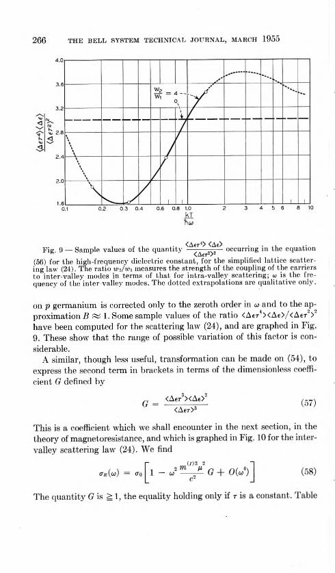
Fig. 9 — Sample values of the quantity occurring in the equation (56) for the high-frequency dielectric constant, for the simplified lattice scatter- ing law (24). The ratio wi/wt measures the strength of the coupling of the carriers to inter-valley modes in terms of that for intra-valley scattering; w is the fre- quency of the inter-valley modes. The dotted extrapolations are qualitative only.

on p germanium is corrected only to the zeroth order in co and to the ap- proximation B ^ 1. Some sample values of the ratio <Aerl><A6>/<Aer">'' have been computed for the scattering law (24), and are graphed in Fig. 9. These show that the range of possible variation of this factor is con- siderable.

A similar, though less useful, transformation can be made on (54), to express the second term in brackets in terms of the dimensionless coeffi- cient (7 defined by

G = (57) <Aer>J

This is a coefficient which we shall encounter in the next section, in the theory of magnetoresistance, and which is graphed in Fig. 10 for the inter- valley scattering law (24). We find

(TK [ an 2 -1

1 - co' 'A-J* G + 0(u') J (58)

The quantity (? is ^1, the equality holding only if r is a constant. Table

TRANSPORT PROPERTIES OF A MANY-VALLEY SEMICONDUCTOR 2C7

IV and Fig. 10 give some typical values, for scattering laws of the form r a Aer or of the form (24).

8. LOW-FIELD MAGNETORESISTANCE

In Section 6 we set up the Boltzmann equation for the steady motion of charge carriers under the combined influence of an electric field E and a magnetic field H, and solved it to the first order in H. We shall now undertake to solve this equation to the second and higher orders in H. The solution has been worked out independently for a number of cases by Abeles and Meiboom,3 Shibuya,3 and Shockley (unpublished). We shall not give all the details of the solution, especially at large H, as many of them can be found in the reference just mentioned. However, to em- phasize some features not brought out in this previously published work we shall review the whole calculation briefly from the beginning.

The relation of theory and experiment in the area of magnetoresistance resembles that for piezoresistance, in that the tensor quantity which is

2.0

2.4

< O 2.0 15

1.6

1.2

1 NV \

0,

A, Wj. w,

1 \

N. N ON — —

1 | 1 1 08 1.0

kT hw

Fig. 10 — Sample values of

<AtT3><At>2

G = <AeT>3 and ,4 =

<Aer3><Aer> <A€T2>2

for I lie simplified lattice scattering law (24). The ratio wo/wi measures the strength of the coupling of the carriers to inter-valley modes in terms of that for intra- vallcy scattering; oj is the frequency of the inter-valley modes. The G curve has been drawn to bo roughly consistent with the smoother -4 curve and the curve of Fig. S. The dotted extrapolations of the curves are intended only to show the ex- pected qualitative behavior.

268 THE BELL SYSTEM TECHNICAL JOURNAL, MARCH 1955

Table IV — Sample Values of the Quantities G and ^4 Defined by (57) and (68), Respectively

Scattering Law „ <Atr1> <A«>! G <A.r>'

<A«t>> <A«r> <A«TS>i

T cc Ae-0-# 2.58 4.01 t a: Ae-0 -5 1.77 1.27 t = constant 1.00 1.00 r cc Ae0-6 1.33 1.09 t cc Ae 2.52 1.28 r cc Ac1-5 5.89 1.58 Form (24), W3/W1 = 4, kT/hco = 1.43 2.77 1.40

0.667 2.70 1.21 0.333 1.92 1.08 0.167 1.52 1.15

simplest to calculate is reciprocal to the one which is directly measured. Thus one measures piezoresistance but calculates elastoresistance. Simi- larly the measured magnetoresistance is a change in the electric field E for given current, whereas the simplest quantity to calculate is the change of the current for given E, i.e., the dependence of the conductivity tensor on H. We shall see below that the neatest way of comparing theory and experiment, at least for small H, is to invert the observed magnetore- sistivity tensor to get the magnetoconductivity tensor, and then compare the latter with theory.

The Boltzmann equation (30), from which we shall start, is

0 = ±eE-Vf/ ± e ^-5 -VP/ - (59) C T

where as before the upper sign is for electrons, the lower for holes, / is the distribution function of the carriers, /<n) the (Maxwellian) distribu- tion in thermal equilibrium, v = Vp€ the group velocity. As in Section 2 we set

/ = /(0) + E ■f(1) + 0(E2) (60)

and neglect higher order terms in E. The resulting equation for f(1) can be written in the condensed form14,15

0 = ± reV p/(0) ± rH-Yf(1) - f(1) (61)

where

Y = - v X VP c

(62)

TRANSPORT PROPERTIES OF A MANY-VALLEY SEMICONDUCTOR 2G9

In the notation of Davis,14 and Seitz,15 f = (e/h2c)Q, while in the nota- tion of Abcles and Meiboom,3 y = (e/c)S2. The solution of (61) can be expressed formally in terms of the reciprocal of the operator (1 ± tH y):

f(,) = ±(1 ± rH• y)-1tcVp/(0) (63)

If we set

(1 it rH-rr1 = 1 + tH-y + (tH-yKtH-y)-• • (64)

we see that the leading term of (63) is just the solution (5) of Section 2 for II = 0, while the next is just the term (33) of Section 6. In other words, the series (64) corresponds to an iterative solution of (59). If we are interested only in the first few powers of H, this iterative solution is as simple as any; at high fields it is better to solve (61) explicitly in closed form, a procedure we shall outline in the next section.

The solution given by (63) and (64) of course applies for any depend- ence of the relaxation time r and the energy e on position P in crystal momentum space. However, we are here interested only in the case where, in each valley i, e is a quadratic function of the components of AP = P - P(<) and where r is a function of e only. For this case some simplifications are possible. For one thing, r commutes with the operator Y, since (62) acting on a function of e contains the factor v X = 0. The expression for the current density j in powers of H has the form

= XI + X + X V^apHaHpEy + " • • (65) y va vaP

where of course (v = for a cubic substance, with o-q given by the equations of Section 2, and similarly , where R is the low- field Hall constant and as in Section 6 5MI,a = ±1 if ^va. is an even (odd) permutation of 123, zero otherwise. To get the contribution of the ?th valley to the second-order "magnetoconductivity" tensor a^ap, we multiply ((50) by icy,,, insert (63) and (64), and sum on all momentum vectors in the ith valley and in unit volume, and on spins. The result is

<Tllyap<'l) = tw; X fWr{vllya'YpVy)Symm (66)

where as usual we have assumed /<0) to be Maxwellian, and where the subscript "symm" means that the expression in parentheses is to be averaged with the expressions obtained from it by permuting a with /3, since only the part of o>a0 symmetrical in a and P has physical signifi-

14 L. Davis, Phys. Rev., 56, p. 93, 1939. " F. Seitz, Phys. Rev., 79, p. 372, 1950.

270 THE BELL SYSTEM TECHNICAL JOURNAL, MARCH 1955

cance. (This symmetrization is not necessary, but simplifies the work by preventing the appearance of meaningless components.)

The explicit evaluation of (66) is a straightforward but tedious exercise in algebra, and will not be given in detail here. However, there are some important properties of the tensor (66) which can be established rather simply. Since the components of v are linear functions of the components of AP, the operator y defined by (62) takes any linear function of the Al\ into another linear function. Therefore the vrfaypv, in (66) is a quad- ratic function of the AP,, , and it is easily seen that this function contains denominators of the fourth degree in the effective masses. Now a quad- ratic function of the AP\ can be written as an effective mass times the energy Ae relative to the band edge, times a function of the direction of AP, dependent only on the ratios of the effective masses in the principal directions. Thus we may write, for example,

Ae v/YalfiV- = ???T7r3 X function direction of AP, mass ratios) (67)

where mU) is the inertial average of the effective masses, defined by (15). Now let the summation on AP be broken up into a summation over values in an energy shell Ae to Ae + f/Ae, and a summation over different shells. The function of direction in (67) will be the same for all the shells, and so we have the result

(i) ^— T? (») &ixvafi (/) 3 / nvafi TTt

where depends on the anistropy ratios of the effective masses in the ith valley, but not on the variation of r with energy, while a is pro- portional to the number of carriers in the valley and to the Maxwellian average of r'Ae.

It is convenient to express the average of r'Ae in dimensionless form by using the quantity (7 defined by (57), namely,

G = <Aer3><Ae>"

<AeT>3

or else the quantity

A = AAv'><AtT> (68) <AtT1>2

Here as usual the angular brackets denote Maxwellian averages as de- fined in connection with (14). We may use (14) to eliminate in{" and the carrier density and if we wish we may eliminate n in favor of /i,, by (39).

TRANSPORT PROPERTIES OF A MANY-VALLEY SEMICONDUCTOR 271

The result is

_ («) /~1 ) r>-/,' (i) t i&OHu ) ri (i) ^ G JNW) ^ JNW)

where oo, m, Mm , ai'c the conductivity, mobility, and Hall mobility, respectively, at /7 = 0, Nv is the number of valleys, and where B ^ 1 is the function of the effective mass ratios defined in (39) and Table III. Summing on valleys i gives

o>o0 = A (^ao—jrjFp,afi = G B2Flll,ad (70)

I'liva/j = -jTjr- t nvap (71) ly V i

Note that F^ap , as defined by (70) or (71), is dimensionless, as are G and A ; F^vap or B' F^ag depends on the geometry of the valleys and the ratios of the principal masses of a valley. We shall see presently how the analysis of experimental data is facilitated by this decomposition of the magnetoconductivity into the product of a scalar factor depending on the behavior of r and a tensor factor depending on the shape of the energy surfaces.

The quantity A defined by (08), like G, is ^1, the equality holding only if r is a constant. Some sample graphs of A and G arc shown in Fig. 10, for scattering laws of the form (24), and some numerical values for this case and for r « At' are given in Table IV. Note that for the ideal case of intra-valley lattice scattering only, a case approximated in very pure material at moderately low T, r = —1^ and A = d/r = 1.27, G = Ott/IO = 1.77. Table V gives values of all the nonvanishing coefficients FHPag " relative to a coordinate system oriented along the principal axes of a valley. The middle rows of Table VI give the F^ag , relative to the crystal axes, for some of the simpler possible arrangements of valleys. The entries were obtained, of course, by comparing (09) or (70) with the results of explicit evaluations of (06). For completeness, Table V also gives the directional factors involved in the contribution a^'" of a single valley to the conductivity tensor in the absence of a magnetic Held, and to the Hall conductivity tensor defined by (34) or (65). All these table entries arc similar to those given by Abeles and Meiboom.'1 However, they have given the unsymmetrized etc. for the eases r = — 12 and +:i/2, in terms of mean free path, absolute values of the masses, and carrier concentration; here we have given the sym- metrized cv,,,? etc. in terms of the directly observable 00 and nH , and for any T(Ae).

sis ^ = H

s I s sis X'

% s ^ s *

1 + * £ +

+ s * * * d £ £ £ + + + * * * J 1 1

J

~r a (M + * H s,

eo s= S.

C1 +

a Tk S

8 •H. S

t, fe.

Ct, fe,

a <

>> c <1

>> c <

* a

H g 8

ic5 3 -o G o O

sc s CD O w

- m v G o hC G ci d »—I

272

-Tl H * I* s ? = H

C-1 + ^v

*=1% S 1 S

At 1* = s 1 s

IC + +

| C-l |

*"1*^ = ~ *=j*H

s 1S C-1 +

= H = S

= H - H -I H - H = H

= H SIS

= H SI 5 * i* H S s

c | ~

= H

- ^

+

8 . f/J > 0 d ci § >

273

274 THE BELL SYSTEM TECHNICAL JOURNAL, MARCH 1955

The qualitative behavior of the entries in Table V is easily understand- able. The Components Faaoa

u> refer to the longitudinal magnetoconduc- tivity when both electric and magnetic fields are in one of the principal directions of the valley, the a direction. Since a magnetic field in such an a direction does not change the a component of the velocity of the car- rier, this longitudinal magnetoconductivity must vanish:

Faaaa{i) = 0.

It is easily verified that, for our model, the principal directions of a valley are the only directions in which the longitudinal magnetoconductivity contribution vanishes. Since the relative longitudinal magnetoconduc- tivity Act/a is necessarily ^ 0, and for a cubic crystal is the negative of the relative longitudinal magnetoresistivity Ap/p, we can conclude that on our model the vanishing of the longitudinal magnetoresistance in any direction is possible, at least for cubic materials, only if the direction in question is a principal axis of all the valleys. It can further be shown, though we shall not give the details here, that lack of constancy of r over an energy shell, far from upsetting this conclusion, merely makes it impossible for the longitudinal magnetoresistance to vanish in any direc- tion.

The nonvanishing magnetoconductance effects can be described in terms of the current due to the force exerted by the magnetic field on the transverse Hall current. This current is proportional to the Hall current and inversely proportional to the effective mass — call it mj* — in the direction normal to the Hall current and to H, this being the direction of the force producing the second-order current. The Hall current, as we have noted in Section 6, is proportional to the zero-order current, hence to the reciprocal of the effective mass mg* in the direction of E, and to the reciprocal of the effective mass ms- h* in the direction normal to E and H.

To employ these ideas specifically, consider first the component aaa^

{'\ which measures the change in current in the a direction pro- duced by a magnetic field in the 0 direction. Here wig* = ma*, mK- = w7*(7 ^ a, 0), nij* = ma*. Thus

Taa00(,) « - —^ * (T ^ a, 0) (72)

the minus sign coming in because the second-order current is in the direc- tion opposite to E. When we insert the mass-dependence of oo///," into (09) and combine with the Faa00U) of Table V, we do in fact find that (Taa00(') contains the masses only as indicated in (72). (The fact that

TRANSPORT PROPERTIES OF A MANY-VALLEY SEMICONDUCTOR 275

Paaw" depends on the masses in a much more complicated way is due to our choice of the defining equation for it, (69): we chose to write this equation so that it involved only the directly measurable quantities a,) and im , Ji'id the dimensionless quantities A and . This choice is the most convenient one for comparisons with experiment, but is less simple conceptually than a choice giving the factor (72).) The remaining independent component, Fa&a&l\ may be analyzed similarly. It repre- sents the second-order current in the a direction due to an E in the /3 direction and an H in the direction midway between a and /3. Here mK* = w/, mB-1* = my*(y ^ a, p), nij* = ma*. The Hall current is weaker by 21 ' than for the previous case, because of the 45° angle between E and H, and since the force producing the second-order current is at 45° to the /3 direction, we must put a second 21'2 in the denominator. Thus

"•w"' * „ , 1 , « = o ^ « (73) 2ma nin my* Imfrnfm *

This, again, can be verified to follow from (69) and Table V. To apply these results to experimental magnetoresistance data in the

region of proportionality to H1, it is necessary, as has been mentioned above, to derive an experimental raagnetoconductivity tensor from the observed magnetoresistance. For a cubic crystal the magnetoresistivity tensor can be described by three constants 6, c (not to be confused with velocity of light), </, defined by

= bH* + c + d (jx'Hx' + j"'Hu' + (74) p//- f r

where Ap is the change of resistivity p due to a small field H, and where the axes are those of the crystal. The equations relating the constants I), c, d to the corresponding constants describing t he raagnetoconductivity tensor have been given by Pearson and Suhl.16 From these equations the components of can lie expressed in terms of the empirical constants h, c, d. The results are tabulated in the last row of Table VI.

If the ratios of these components are compared with the ratios of the corresponding F^cp , one can check the correctness of an assumed model and determine the ratio From the absolute values of the

one can then determine A. A further check is provided if data are available at more than one temperature, since the mass ratio should come out roughly independent of T, while the variation of A with T should

10 G. L. Pearson ami H. Suhl, Phys. Rev., 83, p. 768, 1951.

276 THE HELL SYSTEM TECHNICAL JOURNAL, MARCH 1955

accord with a reasonable picture of the effects of impurity, inter-, and intra-valley scattering on the form of r(A€).

An analysis of this sort has been carried out for n type silicon." For this substance the longitudinal magnetoresistance nearly vanishes in directions of the type (100). From what has been said above, this almost requires that the band structure have valleys on the (100) axes in K- space, and that the relaxation time be practically a function of energy only. Fitting the remaining magnctoconductivity constants gives v\*/mx* ~ 5; this ratio comes out independent of temperature as it should. It agrees with the ratio determined by cyclotron resonance.18

9. HALL EFFECT AND MAGNETORESISTANCE FOR LARGE MAGNETIC FIELDS

As the theory of Hall and magnetoresistance effects for large magnetic fields is rather complicated mathematically, it will suffice for our purposes merely to outline the approach which can be used and to quote a few results without proof. Some of the details can be found in the papers of Abeles and Meiboom' and of Shibuya.3

To treat these we solve the transport equation (61) for the distribution function f(1) and calculate the current density from f(1). This gives the electrical conductivity tensor crM,(H), which can be inverted to give the resistivity tensor . The antisymmetric part of p^ determines a Hall coefficient (in general slightly orientation-dependent),* and the sym- metrical part determines the magnetoresistance.

The solution of (61) can be carried out either by summing the series (64), or directly by guessing that f(1) will be a linear function of the velocity components, with coefficients which are functions of energy. These coefficients can be determined by solving a set of three simultane- ous equations.

As 7/ —> co, the conductivity tensor o>(H) becomes singular, the con- tribution a>(,> of the 7th valley taking the form

a) ne <AeT> Hu.Hv . . ^ v; + mW ln ^ ,

(/) (75)

= m mW + mW+ mW f0r a CUbiC ^

where n is the total density of carriers, Nv the number of valleys, Ae the distance from the band edge, r(Ae) the relaxation time, o-q the conduc- tivity at 77 = 0, mu) the average inertial mass defined by (15), and

17 G. L. Pearson and C. Herring, Physica, to appear. 18 Dexter, Lax, Kip, and Dresselhaus, see Reference 5.

TRANSPORT PROPERTIES OF A MANY-VALLEY SEMICONDUCTOR 277

Hi , Hi, Ih are the components of H along the principal axes of the valley. Summing (75) on i gives a limiting which is still proportional to ; its determinant therefore vanishes, and it cannot be inverted to give the limiting . It turns out that (75) suffices to give the limiting value of the longitudinal magnetoresistance as # —> =c, but that to get the limiting value of the transverse magnetoresistance it is necessary to evaluate contributions to o>(H) of order 1/H'. The limiting Hall coeffi- cient can be obtained from the contributions of order I/II to a>„(H).

The following points are noteworthy; (i) The limiting value of the Hall coefficient as // —► °o is = +(l/nec), independently of the arrange- ment and mass anisotropy of the valleys, and of the dependence of r on energy. Even if r is not a mere function of energy, the same limiting form obtains, (ii) For E parallel to H, the ratio cr(// —> <»)/o-o depends on the arrangement and mass anisotropy of the valleys, but not on the law of variation of r with energy, as long as r is a function of energy only, (iii) For E not parallel to H, both a(H —► co) and (t(H —> co )/o-0 depend on the behavior of r(A€) as well as on the band structure.

ACKNOWLEDGMENTS

I am grateful to the staff of the Institute for Advanced Study for their hospitality during the year 1952-1953, when most of this work was done. Conversations with E. Vogt and W. Shockley have led to improvement of the basic ideas of this paper. Much of the stimulus for it has come from discussions of experiments with F. J. Morin, T. H. Geballe, C. S Smith, T. S. Benedict, and G. L. Pearson. For the ingenuity and labor involved in setting up the various calculations for machine computation, I am indebted to R. W. Hamming and Misses R. A. Weiss and M. M. Segrich.

Appendix A

THE RELAXATION TIME ASSUMPTION

The use of the relaxation time concept represents a great simplification of the Boltzmann equation for all kinds of transport phenomena. To be strictly correct, one ought to describe the scattering processes which the carriers undergo by a transition probability »S,(K, K') defined as the prob- ability per unit time of a transition from an initial state K to a final state in unit volume of wave number space centered on K'. (Conservation of energy will usually limit these transitions to a certain surface in K'-space, so that S will contain a delta function of energy; however, this complica-

278 THE BELL SYSTEM TECHNICAL JOURNAL, MARCH 1955

tiou has no bearing on the remarks of this paragraph.) The Boltzmann equation, for the case of Maxwellian statistics, therefore takes the form

ajw = /^(K)\ + f [/(K'JStK'. K) - /(K)S(K, K')l rfK'. (Al) dl \ dt / Fields J

This is in general an integral equation for the distribution function /, or for the part E-f(I) of/which is linear in the electric field. Our task in this Appendix is to say a few words about the validity of approximating (Al) by an equation of the form

a/(K) = (df(K)\ _ //(K) - /<0)(K)\ (A2)

01 \ dl /Fields \ rfK) /

and to examine the validity of the further approximation t(K) = T(e). We shall give only a rather brief discussion of these questions, however, as a future publication1' will give a more thorough treatment and include a discussion of the solution of (Al) when these approximations fail.

To begin with, let us consider the special class of cases for which

S{K', K) = iS'(K', K*) (A3)

where K* is the state in the same valley as K but with opposite velocity. If (4) is inserted for / in the integral of (Al), the/"" term contributes nothing, and if (A3) is satisfied

JE-f(1)(K')S(K', K) dK' = 0, (A4)

since f(I> is an odd function of velocity while S is even. Therefore, to the first order in E, (Al) reduces to (A2) with

1/t(K) = fs(K, K') dK' (A5)

For collision processes which do not satisfy the velocity-randomizing condition (A3) we may assess roughly the legitimacy of using a T(e) by comparing, for different initial states on the same constant energy sur- face, the mean rate with which scattering destroys the component of velocity in the original direction. This rate of loss of velocity defines a 1 /r which if isotropic is known to lie usable in (A2) for energy-conserving scattering processes in the simple model,1"' and for the many-valley model it is a reasonable presumption, borne out by the more rigorous treatment

19 W. Shockley, Electrons and Holes in Semiconductors (Vim Nostrand 1951) p. 251 et seq.

TRANSPORT PROPERTIES OF A MANY-VALLEY SEMICONDUCTOR 279

of Reference (5, that if this rate of loss of velocity is nearly constant over an energy surface, then (A2) is legitimate with r = T(e).

We shall consider five types of scattering in turn, three by phonons and two by impurities. For the phonon processes, scattering of a carrier from K to K' involves absorption of a phonon of wave vector K' — K, or emission of one with the negative wave vector. The matrix element for such a process is of the fornF"

M(K, K', = Ar"i kM to,. (N + 1),/2 J " "

where N is the occupation number of the lattice mode involved, u is its frequency, and C(K, K') is proportional to the matrix element, between states K and K', of the perturbation of the electronic Hamiltonian due to a static displacement of the nuclei of the lattice, of unit amplitude in this mode. The scattering function »S(K, K') which we have used above is given by

S(K. K') = y E I M(K., K') |! Sle(K) - <(K') ± M (A7)

where 8 is the Dirac delta function and the summation is over absorption (upper sign) and emission (lower sign), and over the various branches of the vibrational spectrum.

(i) Inter-Valley Lattice Scattering. Here the magnitude of K' — K is large compared with the distance of either K or K' from the band edge point nearest it. Moreover, the total change in /)co as K or K' ranges over a constant energy surface will be « kT if the energy relative to the band edge is Therefore the percentage variation of il/(K, K') over such an energy surface will be small. And unless the energy relative to the band edge is extremely small, the surface in K'-space which makes the argument of the delta function vanish will be nearly a constant energy surface. We conclude that »S'(K, K') can be taken to be independent of K and K' when either ranges over a constant energy surface in its valley, and in particular, (A3) applies. Therefore inter-valley lattice scattering is described by a relaxation time which is given by (A5) and is a function of energy only.

(ii) Intra-Valley Scattering by Optical Modes. For a nonpolar crystal this case is essentially the same as the preceding, since the matrix element C(K, K') is substantially equal to its limiting value as K' —> K. For a polar material the longitudinal polar optical modes give a C(K, K') a

2n See, for example, Reference It), p. 520.

absorption (Afi)

emission

280 THE BELL SYSTEM TECHNICAL JOURNAL, MARCH 1955

1 K' - K I-1. In a cubic crystal this contribution is independent of the direction of (K' - K), but if the energy surfaces are anisotropic the variation of C(K, K') with | K' - K ] will suffice to prevent r(K) from being constant over an energy surface.

(iii) Intra-Valley Scattering by Acoustical Modes. Here (A6) and (A7) again apply, but with the simplification that for all but extremely slow carriers the hco in the argument of the delta function can be neglected, since only very low-energy phonons are involved. However, C(K, K7) need no longer be independent of direction. The reason for this is that according to the deformation potential concept,"1 C depends on the strain associated with the lattice mode in question. If only the volume dilatation affected C, as was the case for the simple model, C would be independent of the direction of the phonon wave vector (K — K'), since the dilatation amplitude in a compressional wave of unit dis- placement amplitude is independent of direction. But for a many- valley model both shears and dilatations can produce deformation potentials, and the nature of the shear strain in a shear wave of unit amplitude depends strongly on the direction of propagation. There- fore C may be a function of the direction of (K — K'), in any par- ticular valley.

For a valley whose K(0 lies on a threefold or fourfold symmetry axis of a crystal the deformation potentials due to the different possible types of strains can be expressed in terms of two constants, Sd , Su , which appear in the theory of piezoresistance, Eq. (C6) below, and which are defined thus: Let wr(r = 1 to 6) be the six components of the strain tensor, relative to the principal axes of the valley, the z axis being taken along the symmetry axis of the valley. Then a dilatation in the two directions normal to the symmetry axis (wi = U2 = u/2, Us = 0) produces a band edge shift SdW. A uniaxial shear (iq = ui = —u/2, U3 = u) produces a shift H„w. As will be shown in detail in Reference 6, it is not hard to evaluate the dependence of C(K, K') on the direction of K' — K, in terms of Sd and Su and the elastic constants of the crystal. Thus we can calculate the variation of S(K, K') over an energy surface by (A7), in terms of the constants Sd , S„ , and the anisotropy of the effective mass.

We shall presently exhibit the results of some calculations, made by the procedure just outlined, of how much the rate of loss of initial velocity varies over an energy surface. However, we shall first present an argument that for given deformation potentials, the greatest variation of this quantity may be expected to occur for spherical energy surfaces,

21 See, for example, Reference 19, p. 520 et seq.

TRANSPORT PROPERTIES OF A MANY-VALLEY SEMICONDUCTOR 281

and that usually very little variation will occur for extremely prolate or oblate surfaces. In other words, for almost all values of Hd and Su , the use of a t(c) will be justified for very prolate or very oblate surfaces. Fig. 11 shows the argument. In (a) is shown a spherical energy surface cen- tered on a band edge point on some symmetry axis in K-space. We expect the greatest difference in relaxation time r(K), defined in terms of rate of loss of initial velocity, to be that between a point Ki where the symmetry axis cuts the sphere and a point Ko 90° around the sphere from

. Backward scattering processes for Ki, i.e., those which almost re- verse its velocity, have K' — Ki vectors almost parallel to the symmetry axis, while forward scattering processes, which take K! to a state K' with almost the same velocity, have K' — Ki almost at right angles to the axis. For a carrier initially at Ko, on the other hand, the vector K' — K2 is almost perpendicular to the axis for backward scattering, while for forward scattering it may range from almost parallel (plane of paper) to perpendicular (normal to paper). For this case, therefore, a dependence of the scattering function on the inclination to the symmetry axis will be quite effective in producing an anisotropy of t(K). Now consider the situation for a very prolate energy surface, as shown in (b) of Fig. 11. This figure has been derived from that of (a) by a horizontal extension and a vertical contraction. Now all the dotted lines representing vectors K' - Ki or K' - Kz are nearly parallel to the symmetry axis, and the

SYMMETRY AXIS

BACK FORWARD

(a)

SYMMETRY AXIS

BACK

Fig. 11 — Comparison of intra-valley lattice scattering processes for a valley with spherical energy surfaces, (a), and a valley with highly prolate surfaces, (b).

282 THE BELL SYSTEM TECHNICAL JOURNAL, MARCH 1955

corresponding scattering functions must therefore he very nearly the same. Of course, forward scattering from K, through sufficiently small angles has K' — Ki nearly normal to the axis, and the same is true for backward scattering from Ko in a small range close to 180°. But it is clear that as the energy surface becomes more prolate these cases form a smaller and smaller fraction of the total of possible final states K'. Thus for extreme prolateness r(Ki) —> t(K..). For strongly oblate energy sur- faces most of the K' — K vectors approach normality to the symmetry axis, and a similar conclusion holds. The argument fails if, and only if, the scattering probability practically vanishes for K' — K along the symmetry axis (prolate case) or perpendicular to it (oblate case).

Fig. 12 shows the results of some calculations of t(K2)/t(Ki) carried out by E. Vogt for the worst case, that of spherical energy surfaces, and for an actual case, that of valleys on a (111) axis with = 1.3/.08, the value found in cyclotron resonance experiments on n germanium.5

The anisotropy of the elastic constants has been assumed to be that for germanium. For the spherical surfaces calculations were made for valleys centered on (100) and (111) axes, but the results were found to be in- distinguishable. A comparison of the full curve (spherical surfaces) with the dashed one (prolate surfaces) shows, as expected, that with a highly anisotropic effective mass the anisotropy of the relaxation time is much less than for the spherical case, except near the ratio S,//S„ = — 1. This is the ratio for which modes with wave vectors along the symmetry axis arc incapable of scattering. We conclude that for intra-valley lattice scattering the assumption of a relaxation time dependent only on energy will fail over a considerable range of the deformation potential parame- ters if the effective mass is isotropic, but only over a moderate range near Sd/E.. = — 1 if the effective mass is very anisotropic.

(iv) Scattering by Ionized Impurities. To date the quantum theory of this effect has been developed only on the crude basis of treating the fluctuations of potential due to a random arrangement of ions as a small perturbation on the motion of the charge carriers." The result is that the effective matrix element for scattering between two states K, K' on the same energy surface is a function of K' — K | which is sharply peaked at very small values of this quantity, at least when the density of impuri- ties is not too high. This means that the principal effects come from small- angle scattering, a fact well known in the classical theory of impurity

22 H. Brooks, Phys. Rev., 83, p. 8 & 0, 1951 (contains typographical errors); C. Horie, Toh. U. Sci. Rep. 34, 27 (1950); and C. Herring, unpublished.

TUANSPORT PROPERTIES OF A MANY-VALLEY SEMICONDUCTOR 283

2.8

2,6

2.4

2.2

2.0

1.8

1.6

4^1.4

1.2

1.0

0.8

0.6

0.4

0.2

0 -7 -6 -5 -4 -3 -2 -1 0 1 2 3 4 5 6 7 8

V — u

Fig. 12 — Anisotropy of the relaxation time for intra-valley lattice scattering, as a function of the ratio of the deformation potential coefficient H-i for two-dimen- sional dilatation to the coefficient Zu for uniaxial shear, as these quantities are defined in Appendix A or in Equation (C6). The ordinate is the ratio, for the points Kj and K, of Fig. 11, of the effective relaxation time t defined by t-1 = — (initial velocity)-1 (time rate of change of mean velocity, due to scattering). The elastic anisotropy assumed is that for germanium.

scattering.^1 Now the probability of a collision with a given range of | K' — K | is proportional to the square of this matrix element and to the number of possible final states K' within the given range of distances from K and in a given small range of energy. A little calculation shows that this number is greater when K is near the Ki of Fig. 11(b) than when K is near . Moreover, the fractional loss of the velocity component in the initial direction is greater for a collision at Ki than at Ko. The result

r\

m*!! = m*j_ (100) OR fill) VALLEYS

-\

\

\

—

m*ll/m*1=t.3/o.OB

/(111) VALLEY s

/ / i —

i i

S h •

v/ T

23 E. Conwell and V. F. Weisskopf, Phys. Rev., 77, p. 388, 1950; R. S. Cohen, L. Spitzer, Jr., and P. M. Routly, Phys. Rev., 80, p. 230, 1950; and L. Spitzer, Jr. and R. Hiirm, Phys. Rev., 89. p. 977, 1953.

284 THE BELL SYSTEM TECHNICAL JOURNAL, MARCH 1955

is that carriers near Ki have a much shorter effective relaxation time for impurity scattering than do those near K2.

Thus if the energy surfaces are very anisotropic, the assumption r = r(e) may be expected to be a poor approximation when ionized impurity scattering is important.

(v) Neutral Impurity Scattering. In the simple theory the scattering of charge carriers from neutral impurities in hydrogen-like states is mathe- matically equivalent to the scattering of electrons from hydrogen atoms.24

At the temperatures at which such scattering is important the wave- length of the incident carrier is usually » the diameter of the wave function of the center, so s wave scattering predominates. Therefore the scattering is isotropic. For a many-valley model, however, the situation seems at first sight more complicated, since the effective mass is aniso- tropic, and the centers are not spherically symmetrical. However, it can be shown6 that, at least if the energy of the carrier is low enough, the scattered wave must be describable as an s wave in the space of the transformed coordinates defined by >

= m\* xl2X\ (A8)

In the corresponding momentum space (the i^-space of Appendix B) the surfaces of constant energy are spheres. It follows, that, at least at low energies, neutral impurity scattering satisfies (A3) and is describable by a constant relaxation time.

Appendix B

EQUALITY OF THE ENERGY-SHELL AVERAGES

• \imfV2, }4m3*V32

Choose coordinate axes along the principal axes of the energy surfaces in any given valley. For X = 1, 2, 3, let

n = = APxAmx*)1'2 (Bl)

Then Ae = I e(AP) — 66 | = H S Vx" (B2)

so that the energy surfaces are concentric spheres in y-space. The den- sity of ^-vectors consistent with the periodic boundary conditions is of course uniform, like that of AP. The average of over an energy shell is therefore the average of <p\ over a spherical shell, and thus ob- viously independent of X.

24 C. Erginsoy, Phys. Rev., 79, p. 1013, 1950.

TRANSPORT PROPERTIES OF A MANY-VALLEY SEMICONDUCTOR 285

Appendix C

EXPLICIT CALCULATION OF ELASTORESISTANCE CONSTANTS

Let (T^y be the conductivity tensor of a crystal, defined by the relation

JH = S fTflyEp (Cl)

between current density j and electric field E. Let ua$ be the strain tensor, defined by the relation

dxa = 53 UapXp (C2)

between displacement 5x and initial position x of any point in the body. Then the elastoresistance of any crystal is described mathematically by the fourth-rank tensor da^/diiap , or more conveniently, for a cubic crystal, by the dimensionless tensor —a^du^/dUas , where a is the scalar conductivity in the unstrained state = ad^). The task of this appen- dix is to obtain this tensor by calculating the strain variation of the cur- rent contributions (7), which in terms of components take the form

J, (0 = — E IhT APtO.a

/(0)r(A6(,)) E v.VyEp (C3)

We shall base the calculation on assumptions (a) through (e) of Section 5. Assumptions (b) and (d), regarding existence of a r(Ae) and nondegen- erate statistics, are already contained in (C3). According to assumption (a), we shall neglect any effect of strain on the relations between v, AP, and Ae<0 = | e — €<l) |. Thus we may replace in (C3) by its average Lpyl) over an energy shell, and treat this average for given Ae^ as unin- fluenced by strain:

VuVy 2A^ (t) mi"

0 0

o—o mo

0 0 ms'J

= I L/nu (C4)

When the crystal is strained, the only things that we assume to change in (C3) are the population factor /(0) and the relaxation time t(A£(,)). For some groups of electrons — i.e., values of i and e — the product t/(u) will be increased, and for others it will be decreased. If on the aver- age this product is increased in the valleys whose conductivity tensors are most favorably oriented to the direction of E, and decreased in the

286 THE BELL SYSTEM TECHNICAL JOURNAL, MARCH 1955

others, the total current will be increased by the strain, and vice versa. When assumption (e) of Section 5 is fulfilled, so that two of the m*'s, say mi* and m *, are equal, the tensor (C4) takes the form

^ - ^)] (C5)

as is easily verified by inspection. Moreover, it is easily seen from sym- metry that the only strain components which can alter e'0 in first order are the isotropic dilatation and the shear compounded out of an extension along K(,) and a contraction in both directions at right angles. Mathe- matically expressed, we must have

•j (i) + ZuK^K^/K" (C6)

dUafi

where Zd and E,, are constants independent of the valley i, the subscripts referring to "dilatational" and "uniaxial" effects respectively. The elas- toresistance tensor is, for nondegenerate concentrations,

1 dcr^ e

a I <') I aJV a (J) 1 (i) ./ " | e — cf | ,.(o) or de j (,) T kT dua0

2rJ de^ dua0]

where eF is the Fermi level, ^"'(e) is the relaxation time in the tth valley, and Lm„(') is given by (C5). The second term in brackets in (C7) repre- sents the effect of strain on the transition probability for inter-valley scattering.

We shall now combine and simplify the equations just given. The be- havior of the Fermi level is simple: by assumption (a) of Section 4 it does not shift in shear, and for extrinsic concentrations it shifts with the band edge in compression. Mathematically,

— ~ T - (a+ (cs) dllafi N V j d Ua0 \ 3 /

where Nv is the number of valleys. By virtue of the fact that t, is a func- tion only of Ae and the differences (e"1 — e0)),

(C9)

and it is easily seen that when (C6) and (C8) are inserted into (C7) the Zd terms disappear. Since by symmetry dr^/de'0 = dT(i)/dt3), (C9)

TRANSPORT PROPERTIES OF A MANY-VALLEY SEMICONDUCTOR 287

implies

E ^ = o (cio)

Using this and (C6) and (C8) in (C7), and processing further by (C5), we get

- v v T-u (K*i)KtU) _ 8jA kTa """ V APO)., L AT V Ku)2 3 /

n (>") 7' (»/' (J)l ^ dr Aa A/s .(0), (,•) 4- ac(;) X(,">2 J ■ ^

2ne2Hu f //AV'X'0 Ka(i)Kd

u)\ 8^ r^r\ 3 kTa AT v\ A'02 Ka)2 /.• 9

(Cll)

a O) i,'- (Or' (0 ry- (J) ts (J)\ OT Am A„ Aa A^ \ \^e " A"'2 ' K{')- li

1 _ 1 7113* Wil*

where the upper sign is for n-type, the lower for p, n is the total carrier concentration, angular brackets with a subscript i or i, j mean averages on valleys i or i and j, and angular brackets without subscripts mean Maxwellian averages as defined in Section 2. Substituting from (14) for the conductivity a = nen, we get finally

'3Ai/ 1 //AM

(,)A.(,) KaU)K0{i)\

± kT V\ A'1'2 ' A(i)2 /i 9 , / (C12)

/<*edTU)/de{i)> Am(')A,<') Ka

U)KpU)

v' \ <A6T> A<i)2 ' A(y)2 (Wi* - 7713*)

(77?,* + 27773*)

As in (C7), the first term in square brackets in (012) represents the effect of the strain on the relative populations of the different valleys, and the second term represents the effect on the inter-valley scattering probabilities. We may note the following features:

(1) The trace S„77?M.aa vanishes identically, by virtue of (C9) etc. This means that an isotropic dilatation produces no elastoresistance under the assumptions we are using.

(2) The elastoresistance is proportional to the anisotropy of the effec- tive mass within a valley.

(3) 777,212 = 77)44 vanishes for valleys of the (100) type, while 777,11, = 7711122 (77),, = '"12) for valleys of the (111) type.

(4) The elastoresistance is proportional to l/T at temperatures low enough for inter-valley scattering to be frozen out. Moreover, when AT » the inter-valley hu(ij) of Section 3, the variation of dr./de, with energy

288 THE BELL SYSTEM TECHNICAL JOURNAL, MARCH 1955

At relative to the band edge is easily shown to be one of proportionality to r/At, if impurity scattering is negligible. Under these conditions (probably never achieved by Si and Ge in the extrinsic range) the elas- toresistance is again proportional to l/T1, but with a larger factor of proportionality than at low T.

NOTATIONS

A dimensionless average involving relaxation time, Equation (68)

B dimensionless function of mass anisotropy, Equation (39)

C(K, K') factor in matrix element for a scattering pro- cess K —> K', Equation (A6)

c velocity of light; magnetoresistance constant, Equation (74)

Dij factor in matrix element for scattering from valley i to valley j, Equation (16)

E electric field e electronic charge F^ap factor determining the anisotropy of the mag-

netoconductance tensor Equations (70), (71)

contribution of the tth valley to above, Equa- tion (69)

/ distribution function for charge carriers. /(0) same in absence of perturbing fields, Equation

(1) f(1) etc. change of / in perturbing fields, Equations (4),

(3!), (60) G dimensionless average involving relaxation

time, Equation (57) H magnetic field h Planck's constant/27r j density of electric current K wave number vector for a charge carrier K(l) value of K for the ith band edge point (center

of the fth valley) k Boltzmann's constant

average of v^v, over an energy shell in the fth valley

TRANSPORT PROPERTIES OF A MANY-VALLEY SEMICONDUCTOR 28!)

M{K, K'), Mij

m mx*

ma)

N, Na

Ny n P Qe q R S(K, K')

T t Ucp , Ur V Waiij, a)

W.iij, «) Wl , W2

x, y, z a (when not subscript)

r

Ae

AP, AK

matrix element for lattice scattering, Equa- tion (A6) or (16)

normal electron mass effective mass in Xth principal direction of a

valley inertial average of the m\*, defined by Equa-

tion (15) elastoresistance tensor —cr~ da^/diiap number of quanta (phonons) in a given lattice

mode number of valleys or band edge points number of free charge carriers per unit volume crystal momentum hK. electronic part of thermoelectric power wave number vector for a lattice mode Hall constant transition probability K to unit dK.' at K',

Equation (Al) spin quantum number of a charge carrier absolute temperature time strain tensor components group velocity of a charge carrier transition probability from valley i to valley

j with absorption of a phonon of branch a same but with emission constants of dimension (time)-1, measuring

coupling of carriers to intra- and intervalley modes, respectively, Equations (21)-(23)

rectangular coordinates index labeling branches of vibrational spec-

trum differential operator describing rotation of

distribution by magnetic field, Equation (62)

energy of a carrier relative to the band edge (Ae ^ 0)

departure of crystal momentum or wave vec- tor from valley center

Kronecker delta

290 THE BELL SYSTEM TECHNICAL JOURNAL, MARCH 1955

8^a antisymmetric coefficient = ±1 or 0, Equa- tion (33)

^e, 5v, etc. changes induced by strain e energy of an electron ch band edge energy e(,> energy of the center of the fth valley (nor-

mally = tfe) B Debye temperature k dielectric constant M drift mobility Hi, Hall mobility H,/ , deformation potentials, Equation (C6) ^ transformed coordinate, equation (A 15) p resistivity a conductivity (To conductivity in the absence of magnetic fields

or other perturbations coefficients in the expansion of conductivity in

powers of H, Equation (G5) cTfivafl" contribution of fth valley to magnetoconduc-

tivity r relaxation time of charge carriers tU) ditto for carriers in valley i v transformed wave vector, Equation (Bl) w angular frequency of a lattice mode or an rf

field

New Manufacturing Techniques for

Precision Transformers

for the L3 Coaxial Carrier System

By NORMAN E. EARLE

(Manuscript received November 22, 1954)

The critical Junction performed by the 2504A transformer in the L3 coaxial carrier telephone system necessitated the use of completely new ma- terials and of methods radically different from those usually associated with carrier telephone transformer production. To satisfy operational require- ments, extensive use has been made of parts machined from ceramic and qlass insulating materials which can now be machined to very close dimen- sional tolerances. A description is given of the equipment and techniques which were developed to produce these transformers on a commercial basis, and their effectiveness is evaluated.

INTRODUCTION

Early in 1951 the Western Electric Company set up manufacturing facilities for the production of the L3 coaxial system.* This new system transmits the frequency hand from 0.3 to 8.353 mc over coaxial cables. To counteract the attenuation of these cables, line amplifiers are pro- vided every four miles. The 2504A transformer is used both at the input and output of these amplifiers to couple them to the cable. The system is designed so that the parasitic elements of the transformer are used to help shape the transmission characteristic. Since upwards of 2,000 of these transformers are used in a long cable system, it is neces- sary that the constants of each transformer be held to an extraordinary degree of precision, and that the temperature variation and aging effects be virtually eliminated.

* L. H. Morris, G. H. bovell, and F. R. Dickinson, The L3 Coaxial System, B.S.T.J., 32, July, 1953. A technical description of the 2504A transformer appears on page 891.

291

292 THE BELL SYSTEM TECHNICAL JOURNAL, MARCH 1955

To achieve the desired precision, a radically new type of construction was used for the 2504A transformer shown in Fig. 1. In place of the con- ventional windings, glass cylinders are used, having accurately machined grooves in which the conductor is embedded by a combination of firing and plating processes. Steatite forms are used to provide the housing. In turn, the manufacture of this transformer required the use of new tools and the development of new processes and techniques. The problem the

FERRITE STEATITE C0H6 HOUSING

INNER SHIELD OUTER SHIELD AND WINDING

INNER WINDINGS

FERRITE CORE CORE CLAMP

©

STEATITE CRADLE

Fig. 1A — Exploded schematic of the 2504A transformer.

MANUFACTURING TECHNIQUES FOR PRECISION TRANSFORMERS 293

d

Fig. IB — 2504A transformer.

engineer of manufacture had to solve, therefore, was how to set up to produce 2,000 such transformers a year on a capacity basis.

Table I gives a comparison of the structural details of the 2504A as compared to those of a carrier transformer of conventional design.

The new materials, in addition to having stability, low loss, and good insulating properties, can be held to very close mechanical tolerances, a condition which makes it possible to obtain the degree of electrical

Table I — Comparison of Structural Details of 2504A with Those of a Conventional Transformer

Part Conventional Transformer 2504A Transformer

Core Winding form . .

Windings

Shielding

Coil enclosure . . .

Permalloy powder Molded or fabricated plastic

part Machine-applied insulated

drawn copper wire Copper or tin foil

Metal or plastic container

Manganese-zinc ferrite Threaded cylinders of special

glass Plated copper embedded in

special glass forms Fired silver on special glass

forms Steatite housing and cradle

294 THE BELL SYSTEM TECHNICAL JOURNAL, MARCH 1955

precision required, once the techniques for performing the mechanical operations have been developed.

In the gage making art, equipment has been available for many years for grinding threads to tolerances comparable to the ,0.031 ± 0.0005" limits on the wall thickness between the inner diameter and the bottom of the threads of the glass form for the outer winding of the transformer and the 0.0005" concentricity limits on the cylindrical inner and outer surfaces of the same part. However, considerable development was necessary before techniques could be worked out to hold such tolerances on fragile, thin-walled glass parts without excessive breakage.

Application of silver to the inner surfaces of the middle and outer forms, shown on Fig. 2, and the plated copper windings to the inner and outer forms presented similar problems. The difficulty was not the newness of the art, but the unusual surfaces on which the silver had to be applied, and the uniformity required in order to obtain the precise control of leakage fluxes and interwinding capacitances that was neces- sary to maintain the desired shape for the transformer's transmission characteristic.

Further problems were encountered by the manufacturing engineer in measuring some of the mechanical dimensions ot the parts and some of the electrical characteristics of the completed transformer to the ac- curacy required and in arriving at a satisfactory correlation between changes in mechanical dimensions and the resultant changes in electrical properties that in the end were the characteristics that had to be held precisely.

MACHINING OF THE GLASS COIL FORMS AND THE CERAMIC CRADLE AND HOUSING

With the exception of a honing operation on the inside diameters of the coil forms and the final dressing operation after the parts are copper plated, all machining operations on the cradle and housing and on all three coil forms for the 2504A transformer are done on special grinding machines equipped with fine grit bonded-diamond wheels.

The configuration of the winding forms is shown diagrammatically in Fig. 2. These forms were originally made from fused quarts; but later, extensive tests showed that a cheaper 96 per cent silica glass, could be used interchangeably with the quartz. While the material is very hard, the parts themselves are thin and consequently fragile and easily dis- torted; so easily, in fact, that they can be distorted by more than the specified tolerance simply by holding them between one's fingers. This

MANUFACTURING TECHNIQUES FOR PRECISION TRANSFORMERS 295

factor, together with the close dimensional tolerances including the concentricity requirement of ±0.0005" on the outer winding form, made it imperative that tubing appreciably thicker than the finished product be used as the raw material for making the part. This made possible accurate honing of the inside diameters, used as the base point for hold-

LEAD-IN GROOVES

FIRED SILVER INNER SHIELD

SPACING SHOULDER

EMBEDDED ~—PLATED COPPER

INNER WINDINGS ^0

■Oo

nO3 SPACING

-'"SHOULDER

cc3 *0- 031

+ 0.0005

00J >0-

o

FIRED SILVER^ OUTER SHIELD

EMBEDDED PLATED COPPER

OUTER WINDINGS

Fig. 2— Composite view of winding forms, embedded copper windings and fired silver interwinding shields.

296 THE BELL SYSTEM TECHNICAL JOURNAL, MARCH 1955

ing all other dimensions of the parts to the precise dimensions required. Though the specified tolerances on these dimensions were wider, in actual practice, it was found that holding the inside diameters to plus or minus 50 millionths of an inch made it much easier to meet the limits on other dimensions, particularly the highly important wall thickness dimension of the outer form.

0.728 +0.0001

♦

ADJUSTING WEDGE ■

DIAMOND HONE

STEEL MANDREL

Fig. 3 — Honing inside diameter of coil form.

MANUFACTURING TECHNIQUES FOR PRECISION TRANSFORMERS 297

In preparing the tubing for this operation, the-hiateriai is pre-shrunk in a plastic state at elevated temperatures around an accurately ground mandrel with the result that the bore is reduced to within 0.001" to 0.002" of its final size. The keyway required in the inner form is formed by the same process. No machining of this slot is required.

Rough grinding of the outside diameters to ±0.001" and facing the

|<-0.760 ± 0.003->|

A 0.060

±0.003

=1

■*-0.816 ± 0.003-->1 <- 0.641 ± 0.003—>l

0.060 + 0.003

0.015 ' MAX. RADIUS

35° io'SO"

±- 35° +0 30

V ^o.oes

Fig. 4 — Cutting slots in end of inner form.

298 THE BELL SYSTEM TECHNICAL JOURNAL, MARCH 1955

MANTJFACTURING TECHNIQUES FOR PRECISION TRANSFORMERS 299

ends to meet the ±0.003" tolerance for the overall length of the parts presented no particular problems. However, the use of an Arnold gage to give a continuous indication of the outside diameter during grinding of the parts was novel to coil manufacturing.

Three special machines, developed early in 1951, make the notching, slotting and trimming, necessary in forming the lead in grooves and tabs of which they are a part, a relatively easy operation, despite the fact that the tolerance in their angular location is better than ±1°. These ma- chines — one of which is shown pictorially in Fig. 4 — contributed materially to the uniformity of the product, a factor of utmost impor- tance in controlling the internal parasities of the transformer.

Undercutting of the inner and middle forms for the spacing shoulders on these parts is a straight forward cylindrical grinding operation. Toler- ances on the width of the shoulders are ±0.003", while those of the diameter of the parts are ±0.001".

Grinding of the threads on the inner and outer forms — the final operation prior to application of the plated copper windings — as had been anticipated — turned out to be a major manufacturing problem. Production of an experimental lot of transformers on a specially equipped toolmakers' lathe indicated that the best way to obtain the uniform control desired was through the use of an automatically cycled com- mercial thread grinder. Other methods, including a novel approach in which the threads were formed by a high-frequency vibration process using a powdered abrasive cutting agent, were either too slow or in- herently did not have sufficient controls to yield the required uniformity. Even with the automatically cycled commercial thread grinder, con- siderable development was required to work out the required techniques for the process and only one supplier could be found who would under- take to work out the proposed machine modifications involved.

One of the problems was to adapt the grinder to permit use of a metal bonded in place of the resinoid bonded diamond or silicon carbide wheel conventionally used for thread grinding. Factors leading to the selection of the metal bonded diamond wheel were (1) the necessity for holding as nearly square a thread as possible — in practice a 141 2° Acme thread with 0.0015" maximum radii in the corners — and (2) the extremely hard abrasive nature of the material being worked. To permit use of these wheels, specially designed silicon carbide scrubbers had to be provided, built in to automatically dress the wheel to the shape required after completion of a predetermined number of parts.

Selection of the proper grain size for this wheel was also critical. Wheels much coarser than 300 grit — a size so fine it could he used to produce a

300 THE BELL SYSTEM TECHNICAL JOURNAL, MARCH 1955

high polish on metal parts — caused excessive chatter and breakage of parts when used to grind fine threads on glass.

The speed of approach and retraction of the wheel — controlled by a specially shaped forming cam — also had to be carefully worked out, not to minimize parts breakage alone, but to control thread over-

LEFT HAND THREAD 68+0.2 THREADS PER INCH

EXACTLY 50 TURNS

0.081 ±0.002

0.79O ±0.0005

0.0070 ±0.0006

14.5° ^ /* 14.5°

0,0015 MAX. R

WORK

GRINDING WHEEL WORK

ARBOR

0.0004 CLEARANCE

Fig. 6 — Cutting thread in outer winding form.

MANUFACTURING TECHNIQUES FOR PRECISION TRANSFORMERS 301

run, a factor affecting one of the transformer's parasitic interwinding capacitances.

Simultaneous removal of copper and glass in the final dressing of the parts after copper plating of the forms for the transformer windings re- quired the selection of a wheel which could cut with very light pressure so as not to break the brittle glass form and at the same time not load up with copper from the windings. The most practical unit found for this operation was an "I" bond vitrified silicon carbide 220 grit wheel. Wheels with a stronger bond tended to cause excessive parts breakage, while softer ones broke down so rapidly that the required tolerances could not be held.

To provide as desirable operating conditions as possible, all of the grinding machines with the exception of one used for rough work were located in a dust free air-conditioned room in the basement of the building. In the case of the thread grinder, it was found necessary to take the further precaution of warming up the machine for a minimum of one and one-half hours prior to using it and providing more rigid guards in place of standard equipment in order to reduce vibration.

Machining of the steatite cradle and housing for the transformer presented problems of a similar nature. However, tolerances were not quite as critical and more information was available on commercial machining practices. As a result, not nearly as much development was required as on the glass winding forms. Procurement of unground parts sufficiently non-porous to avoid spalling and breakage of the housings, during firing after application of the sprayed silver shield on its inner surface, has been troublesome.

SILVERING AND PLATING OF THE GLASS AND CERAMIC PARTS

The inner surfaces of the ceramic coil housing and those of the middle and outer glass winding forms must be silvered for shielding purposes. The outer surfaces of the inner and outer coil forms are similarly proc- essed to provide a base for the plated copper which, in combination with the silver, forms the actual coil windings.

It was imperative that these coatings be uniform in density and thick- ness particularly those on the inner surfaces of the coil forms. Thin non- uniform coatings result in intolerable variations in leakage inductance and interwinding capacitance, while excessively thick ones cause as- sembly difficulties. Other prerequisites were:

1. A strong dependable bond to the glass and ceramic surfaces. 2. Careful masking and process controls to insure that conductive

302 THE BELL SYSTEM TECHNICAL JOURNAL, MARCH 1955

1 1 1 1 1

o.aos ±0.001 i i i i i ±

GRINDING WHEEL DRIVING DOG

ADJUSTING NUT /

-r ARBOR

s SPRING

'-WORK SPINDLE DRIVING

PIN WORK SPINDLE

Fig. 7 — Grinding outside diameter of coil form.

MANUFACTURING TECHNIQUES FOR PRECISION TRANSFORMERS 303

material did not splatter onto critical areas where it might cause corona discharges while in service.

The silvering agent used was a finely ground silver powder suspended in a volatile organic solvent with small amounts of resin and glass frit. Sprayed on under controlled conditions in specially developed machines, the organic material is driven from the mixture by firing at 1250oF in a continuous belt furnace. At this temperature, the glass frit melts and wets the surfaces, bonding the silver securely to the glass and ceramic parts. Thickness of the coating is controlled by weighing control parts on a chain-o-matic laboratory balance before and after spraying and again after firing. Uniformity is improved by the application of multiple coats. However, not more than two can be used because of devitrification which results if quartz or high silica content glass parts are repeatedly fired at high temperatures.

In the early stages of production, the shield consisted of copper plating over fired silver coatings. This method required extra plating processes and prolonged the exposure of the parts to the plating solution. Since such solutions can attack the silver glass bond of the parts, plating of the shields was abandoned. To improve the continuity and conductivity of the coating, the parts are burnished in a specially developed machine which in a carefully timed cycle draws the inner surfaces of the parts spirally across the periphery of a rapidly rotating wire brush. Very good results have been obtained with the present process, the leakage im- pedance variation being reduced to plus or minus one-half of one per cent.

The threads which form the windings of the transformers are produced by plating copper on top of the silver fired on the outer surfaces of the inner and outer forms. The problem confronting the manufacturing engineer in this operation was that of applying as homogenous as possible a trapezoidal ribbon of copper in the narrow grooves on the outer surfaces without loosening the silver bonded to these forms.

This meant that the parts must not be permitted to remain in the plat- ing bath any longer than absolutely necessary and that a well controlled process must be used to avoid bridging of the copper at the top before the groove is completely filled in the middle. To solve this problem, a plating process was used where initially the parts are given a flash of copper in a copper sulphate bath to protect the fired silver from attack by the copper fluoborate bath, subsequently used to permit rapid appli- cation of the heavy plating required. This flash effectively protects the silver from attack by the latter solution. To keep a fresh solution in the threads and to provide a uniform coating, the parts are rotated briskly during the plating operation. Because the quantity of parts being proc-

304 THE BELL SYSTEM TECHNICAL JOURNAL, MARCH 1955

essed has not been sufficiently great to justify provision of a plant to provide continuously fresh plating solution, constant vigilance was re- quired to keep impurities out of the solution. For this reason the anodes were enclosed in closely woven plastic bags and the solution was purified daily by filtering after treatment with activated carbon.

Microscopic analysis of etched cross-sections of the threads and dc resistance measurements on the overall windings indicated that ex- ceptionally good results were being obtained by this process. Control is maintained by a continuous check of the winding for dc resistance.

PHYSICAL AND ELECTRICAL MEASUREMENTS

The performance of the transformer in its final state depends to a great extent upon the accuracy to which dimensions of the winding forms have been held. In fact, investigation has shown that half of the total varia- tions in the overall transmission characteristic of the transformer can be attributed to variations in the dimensions of the outer form. Dimen- sional measurements on these parts thus becomes an extremely im- portant consideration. Critical dimensions are the inside diameters of the three forms, wall thickness of the outer form at the root of the thread, and outside diameter of the inner form. Standard air, dial indicator and electronic gages provided have proven adequate for measuring these dimensions to the close tolerances required. Measurement of the wall thickness of the outer forms at the root diameter, however, has been very troublesome. The problem here is complicated by the fact that the measurement has to be made from a cylindrical surface in one plane to a point at the bottom of a narrow thread in a plane at the helix angle of the thread. At this point, the Acme thread is approximately 0.004" wide in- cluding the 0.0015" radii in each corner. The use of an optical com- parator even at 100X magnification proved impractical because of the curved surfaces involved. After trial of this and other methods, some of them quite elaborate, it was found that the simple expedient of inserting a thin diamond blade in the thread and comparing the distance from the bottom of the blade to a circular rod supporting the cylindrical form with a flat ground carbide thickness gage gave the most consistent results. A diamond blade was used because it was found that the thin edge of the blade wore rapidly even with carboloy. A diamond edge lasts about six months. Results indicate that an accuracy of ±0.0002" is attainable. While this accuracy is consistent with the ±0.0005" limit on this dimension, greater accuracy would be useful in setting control limits. The strain gage used as the measuring instrument can be read to much greater

MANUFACTURING TECHNIQUES FOR PRECISION TRANSFORMERS 305

accuracy. However, to date, no means has been found to obtain an im- proved method for contacting the surfaces to be measured.

Other mechanical measurements, while made to a degree of precision unusual in the coil manufacturing field, are of more or less routine nature and no particular difficulty was experienced in providing equipment capable of making measurements to the accuracy required.

The transformer was designed to require no adjustment to meet its specified electrical requirements, even though the requirements for the transformers' transmission characteristics were closer than those on all but a very few other designs even after adjustment. The phase and transmission set* provided for making these measurements is capable of a high degree of precision. However, to obtain the needed precision, an unusual amount of maintenance is required, the set being taken out of service for one day a week for this purpose. The set proved very useful in arriving at a correlation between transformer variations and those of the amplifier stage of which it is a part.

Special sets used for measuring the leakage impedance, the capacitance across the high impedance winding and the capacitance from the high voltage end of that winding to ground were very useful in controlling variations in the transformer.

CORRELATION BETWEEN TRANSFORMER ELECTRICAL AND MECHANICAL RE- QUIREMENTS

The purpose of electrical tests is to insure proper performance of ap- paratus in its end use and to provide process controls as an aid in meeting overall manufacturing objectives. Because of its unique mechanical construction and the precision to which the dimensions of its com- ponents are held, the first order causes of variation in the parasitic in- ductances and capacitances used to shape the transformers' transmission characteristics are under close control. Certain secondary causes of varia- tion show up, however, which are quite different from those of the average carrier transformer. This is aggravated by the fact that the transformer is part of the amplifier feedback circuit and in consequence, certain parasitic capacitances have a much greater effect than they would have if the apparatus were used in a less complicated circuit.

Statistical control charts were very useful in meeting the test objec- tives on the 2504A transformer. Continuous control charts showed small

* D. A. Alsberg and D. I.eeil, A Precise Direct Reading Phase and Transmission Measuring System for Video Frequencies, B.S.T.J., 28, p. 221, April, 11)49, and D. A. Alsberg, A Precise Sweep-Frequency Method of Vector Impedance Measure- ment, Proc. I.R.E., 39, p. 1393, Nov., 1951.

306 THE BELL SYSTEM TECHNICAL JOURNAL, MARCH 1955

but very noticeable leakage inductance variations as measured at seven megacycles. Discovery of the reasons for the variations was not as ob- vious. Calculation showed that the possible contribution of the various factors in a commonly used formula for the total leakage inductance referred to one of the windings

_ 10.GN2li'2 Ct + a) henries be2 X 109

where N = turns in the winding I = mean length of turn for all windings c = number of insulation spaces I = thickness of insulation space

a = height of window opening b = width of winding

was too small to account for the variations experienced, small though they were by comparison with those of conventional transformers. The num- ber of turns in the windings and the number of insulation spaces being automatically fixed and charts of other factors indicating adequate control focused attention on the assumptions used in arriving at the formula expressed above. One of these — the assumption that the leakage flux is uniform and parallel to the axis of the core — provides the clue to the variations. A certain amount of flux must intercept the shields and set up eddy currents. Differences in the effective thickness of the shields were found to be major contributors to leakage impedance varia- tions. This led to the establishment of the elaborate controls on the spraying process described earlier in this article.

Control of parasitic capacitances presented a somewhat different prob- lem. While the interwinding capacitances of the transformer are com- plexly interrelated, charts kept for control purposes showed fair correla- tion between the wall thickness of the outer form and the capacitance across the high impedance winding. Possibly greater correlation could have been obtained if the average wall thickness could have been arrived at through a weighted integration process. Despite the fact .that the data were not entirely adequate, a number of irregularities in mechanical processes were discovered as a result of the keeping of control charts on this characteristic. Typical was the discovery of a worn condition on a carbide rod used for contacting the inner cylindrical surface of the outer winding for one of the gaging operations. Through continued use, a crescent shaped valley had been lapped out of the middle rod by the abrasive action of the glass parts in inserting them in the gage. As a

MANUFACTURING TECHNIQUES FOR PRECISION TRANSFORMERS 307

result, a condition that might have gone undetected for some time was corrected before a large quantity of expensive parts were completed.

Numerous correlations similar to the two just described have been helpful in establishing manufacturing procedures on the 2504A trans- former and have contributed a great deal to the setting up of satisfactory process routines.

ACKNO WLEDGM ENTS

The co-operative spirit prevalent throughout the period while the manufacturing techniques for this unusual transformer were being worked out, a few of which have been described herein, has been very gratifying. Contributing to this were people in a wide variety of de- velopment and research groups at Bell Telephone Laboratories as well as many individuals in the engineering and operating departments of the Western's manufacturing organization. Among the many individuals involved, the efforts and suggestions of G. Bittrich, W. L. Brune, F. R. Dickinson, W. F. Janssen, C. W. Thulin, and A. W. Treptow of Bell Telephone Laboratories, and G. V. Craddock, A. Habif, F. J. Sweeney, A. R, Swenson, H. S. Wahlberg and operating supervisors P. Ferguson, L. G. Holt and R. H. Onyon of Western Electric's manufacturing organization were particularly helpful. With their help, processes at the end of the second year of manufacture are well stabilized with a defect rate in the final state of less than 5 per cent and a process breakage rate of tolerable proportion, a remarkable achievement considering the precision and unique processes involved.

Development of Reed Switches and Relays

By O. M. HOVGAARD and G. E. PERREAULT

(Manuscript received November 29, 1954)

Improvements in the operating speed, efficiency, compactness and contact reliability of relays may he obtained from the application of sealed-in-glass reed switches. This paper is an account of the development of such switches and relay designs suitable for their use. Because of the close dependence of contact performance and switch operating characteristics upon process methods their development has been an important part of this project.

I — Reed Switches

Switches are those basic circuit elements of a telephone system which make it feasible to establish the connections desired by telephone users. To permit remote operation, switches in the telephone plant are usually electromechanical devices and they are used to select and establish needed talking paths. Since switches are used in large numbers their manufacturing and operating costs have a significant impact upon tele- phone economics and for this reason the development of switching appa- ratus receives much attention.

HISTORICAL

In 1936 the availability of new magnetic alloys prompted a study of improved means for the operation of switching contacts. As a part of this work there was conceived an extremely simple magnetic structure giving promise of excellent electromechanical efficiency, unusually high operating speeds and lending itself to very compact designs. This paper is an account of the development of this basic concept to the point of practical application in the Bell System.

The basic concept is shown in Fig. 1. Two flat reeds of magnetic ma- terial are supported as cantilevers with their free ends overlapping and separated by a small gap. Surrounding the reeds is an operating coil so

309

310 THE BELL SYSTEM TECHNICAL JOURNAL, MARCH 1955

placed that the overlap of the reeds is at its center. When the coil is energized the flux in the gap pulls the reeds together. The reeds perform the double function of a magnetic operating gap and a contact pair with which to close and open an electrical load circuit. This is a radical de- parture from the classical relay wherein the operating gap is external to the energizing coil and the armature operates the electrical contacts through mechanical linkages. The result is improved electromechanical efficiency through reduction in magnetic leakage and increased operating speed as the result of smaller displacements and moving masses.

In practice the reeds are supported by sealing them into the ends of a glass tube. This provides a structure sufficiently stable mechanically to assure the maintenance of the critical gap between the reeds and gives

OPERATING COIL

INSULATING CLAMP

MAGNETIC REED

Fig. 1 — Basic reed switch concept.

excellent electrical insulation between them in their unoperated position. Furthermore, by providing a hermetic seal around the electrical con- tacts it frees them from the effects of environment. This is of fundamental importance since corrosive or dirt-laden atmosphere is a major cause for expensive contact maintenance.

Initial embodiments of this design concept were not as simple as indi- cated in Fig. 1. Materials having optimum magnetic characteristics do not in general make sound gas tight seals to available glasses, nor do they serve satisfactorily as electrical contacts if exposed to the air. Con- sideration of these factors led to the design shown in Fig. 2.* Reeds of the desired magnetic material are welded to supports of materials which will seal to glass and serve as electrical connections to the contacts. One of these supports is a rod, the other is a metal tube. After the switch has been assembled it is evacuated through the tube and filled with the de-

♦ U. S. Patent 2,289,830.

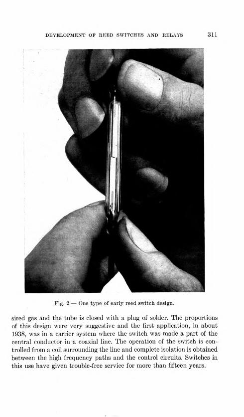
DEVELOPMENT OF REED SWITCHES AND RELAYS 311

a.-

L- - - ' iTt

Fig. 2 — One type of early reed switch design.

sired gas and the tube is closed with a plug of solder. The proportions of this design were very suggestive and the first application, in about 1938, was in a carrier system where the switch was made a part of the central conductor in a coaxial line. The operation of the switch is con- trolled from a coil surrounding the line and complete isolation is obtained between the high frequency paths and the control circuits. Switches in this use have given trouble-free service for more than fifteen years.

312 THE BELL SYSTEM TECHNICAL JOURNAL, MARCH 1955

It was natural that this radically new switching element should find important military application because of its independence of such en- vironmental factors as corrosion, dirt and altitude. Under the impetus of World War II a dozen or more designs were evolved for specific appli- cations and much was learned about the basic design as well as the process problems of manufacture. This experience demonstrated that with its inherent compactness, efficiency and operating speed this switch could find broader application in the telephone plant and its develop- ment for this purpose was undertaken. To fully attain this goal the design and manufacturing process must result in a cost comparable to that of a pair of nickel silver springs carrying the customary precious metal contacts and the operating life of the switch should approach one billion operations for electrical loads up to one-half an ampere.

DEVELOPMENT

The operating characteristics of a switch, i.e., the ampere turns to cause it to close, to hold it closed or let it open, depend upon the mag- netic characteristics of the reeds, their dimensions, overlap, separation in the unoperated state and the amount of contact plating. These factors also influence the relationship between operating speed and power and thus affect switch efficiency. In addition to these design factors such process matters as the flatness of the reed surfaces, precision of their alignment and the accuracy with which the unoperated gap is established determine the tolerances which can be placed upon the switch operating characteristics. Switch and process design are inseparable and the degree of development of the latter becomes controlling in the determination of attainable switch operating tolerances. Therefore, studies were made to explore both of these phases of reed switch development.

The relationship between the operating characteristics and the un- operated gap of an experimental reed switch is shown in Fig. 3 for several values of reed overlap. As the gap is increased, the reed deflection and the magnetic pull required to close the switch increase. Therefore, the flux density in the gap must be increased correspondingly, and, as shown by the curves, the onset of magnetic saturation of the reeds and in- creased leakage across the gap cause the relationship between the ampere turns required to close the contacts and the switch gap to become in- creasingly nonlinear. Magnetic saturation of the reeds will therefore determine the maximum gap at which a given switch design can be closed. The restoring forces to separate the reeds, i.e., release the switch, when the operating flux is removed are obtained from the deflections of

DEVELOPMENT OF REED SWITCHES AND RELAYS 313

OPERATE RELEASE

OVERLAP 0.100

z 0.070

.050

OVERLAP 0.100 _

0.070

0.060

0.008 0.009 0.010 GAP IN INCHES

0.011 0.012

Fig. 3 — Operating characteristics of a reed switch versus the gap in the un- operated switch.

314 THE BELL SYSTEM TECHNICAL JOURNAL, MARCH 1955

the reeds upon switch closure and therefore are proportional to the un- operated switch gap. A switch will open when the restoring forces exceed the magnetic pull between the reeds. Although under these conditions the flux density in the reeds and the gap leakage are low, there are mag- netic saturation effects at the surfaces of the reeds which cause the

ISO

170

160

150

140

130

120

110

W too IT D W 90 a LU a | 80

70

60

50

40

30

20

10

0 0 0.02 0 0.04 0 0.060 0.080 0.100 0.120

OVERLAP IN INCHES Fig. 4 — Operating characteristics of the same reed switch as in Fig. 3 versus

the reed overlap.

/

i 1

RELEASE /

/

/

/

/

/ GAP 0.0I0> /

/

0.0 OB^"

0.0 36^,

^ " ^O.OIC

.... -0.008

0.006 " . —— — —

DEVELOPMENT OF REED SWITCHES AND RELAYS 315

relationship between switch release and switch gap to be approximately linear. The relationships for the same reed design as a function of reed overlap is shown in Fig. 4. The shape of the operate characteristic arises from the decrease in percentage of leakage flux around the gap and the decrease in the gap flux density as the gap area is increased. These factors have opposing effects upon the switch ampere turn operate value, the former predominating at small overlap, the latter for large overlap, and therefore the characteristic exhibits a minimum when the reluctance of the working gap equals that of the remainder of the magnetic circuit. The extreme curvature for the 0.010" gap at the higher values of overlap is caused by magnetic saturation of the reeds. The rising character of the release curves is due to the decrease in flux density as the overlap is increased. This results in less magnetic pull and a higher switch ampere turn release value.

The contacts of reed switches are subject to electrical erosion which may take the form of a buildup on one reed associated with a pit on the mating reed. As with ordinary contacts, such buildups can give rise to mechanical locking of the reeds causing failure of the switch to open. The reeds may also become welded upon closure by excessive currents or capacitive discharges from the electrical load circuits. The restoring forces of the reeds are counted on to rupture such locks or welds as may occur within the specified limits of contact operation. Since the restoring forces are proportional to the switch gap better margins against locking or welding will be provided with larger switch gaps. However, the charac- teristics described above show that increases in the gap rapidly decrease the switch magnetic efficiency. Furthermore, the increase in the slope of the characteristic indicates that, for larger gaps, we should expect greater dispersion in the operate characteristic for a given precision in establish- ing the nominal gap in manufacture. Small gaps look attractive from the standpoint of switch efficiency but are more difficult to establish in switch assembly. In addition, the by-products of contact electrical ero- sion arc magnetic and tend to collect in the switch gap and cause trouble if this is too small. The selection of the gap size for a given switch design is a compromise of these factors of switch application and process design. The reed overlap is selected to fall at the minimum point of the charac- teristic which at once provides maximum switch response and minimum sensitivity to manufacturing variations in overlap.

In the assembly of a reed switch the seals are the anchorage for the reeds and their location determines the effective cantilever lengths and the stiffness of the reeds, and the lengths of the seals influence the rigidity of the reed anchorage. Thus it is important that the sealing technique

316 THE BELL SYSTEM TECHNICAL JOURNAL, MARCH 1955

permits good control of this process step. Since a switch is only about three inches long the close proximity of reed holding chucks and mecha- nisms for aligning and spacing the reeds make the open flame sealing techniques of the vacuum tube art unattractive. Furthermore, with open flame techniques it would be difficult to obtain adequate control of seal

HEATER COIL

ELECTROMAGNET POLE FACE

c

t

— COMPLETED SEAL

CHUCK

MICROMETER CONTROL

Fig. 5 — Early laboratory type machine for assembling reed switches.

DEVELOPMENT OF REED SWITCHES AND RELAYS 317

location and dimensions. A new method had to be conceived and this has taken the form of an electrically heated coil of resistance wire sur- rounding the ends of the glass envelope. A laboratory facility for assem- bling switches is shown in Fig. 5. One of the reeds has already been sealed into one end of a glass envelope by a previous operation and this sub- assembly is shown mounted in position for receiving the second reed. The glass tube of the switch is to the right of a prism used in the process of aligning the reeds. The seal already made can be seen projecting from the mechanism just below a spring clip providing an electrical contact to the reed support. The lower end of the glass tube projects into and is closely surrounded by an electrical heater coil. Below the heater is a chuck for supporting the reed about to be sealed into the switch. This chuck is of magnetic material and can slide on a steel surface which is also the pole face of an electromagnet. The chuck may be moved in rotation and translation until the reeds are in alignment as determined by visual inspection through the prism after which it is locked in position by energizing the electromagnet. The chuck and its support are fastened to a carriage which can be moved in translation under control of a micrometer having a calibrated head, and this is the means for establish- ing the desired switch gap. After this operation the heater coil is ener- gized to make the seal. The temperature of sealing is controlled by the voltage applied to the heater coil and the time of application by an electrical timer. Most of the heat is transferred to the glass by radiation and the temperature of the glass is raised sufficiently so that its surface tension can overcome its viscosity. Surface tension draws the open end of the glass body inward until the glass comes into contact with and wets the metal oxides of the reed support thereby effecting a seal. In addition to performing well the sealing function, this method also per- mits control of the seal cooling so as to provide a desirable strain relieving anneal of the glass.

In developing the process for making a metal-to-glass seal it is neces- sary to obtain detailed knowledge of the thermal characteristics of the materials to be used as well as the temperature-time phenomena in- volved. In the range between room temperature and the softening point of the glass the coefficient of expansion of the metal is essentially linear and its magnitude depends on the composition of the alloy. In this same range the coefficient of the glass is nonlinear but it is possible to select metal and glass combinations which will exhibit low seal strains after the combination has cooled to room temperature. At temperatures be- tween the softening point of the glass and room temperature a seal will be subjected to varying degrees of stress depending upon the choice of

318 THE BELL SYSTEM TECHNICAL JOURNAL, MARCH 1955

alloy composition and these stresses may become serious enough to cause the seals to crack. The stresses at intermediate temperatures may be reduced by suitably annealing the seal but they can become greatly aggravated if the thermal characteristic of the sealing machine does not permit the metal and the glass to cool at approximately the same rate. In consequence the thermal characteristics of the means for supporting the reeds during sealing, the rate of cooling of the electrical heater coils and the susceptibility to the effects of drafts are all matters which must be studied in the design of the sealing process.

To obtain switches with operating characteristics that are predictable within acceptable tolerances it is necessary that the reeds be parallel to each other. This requires that the reeds be flat and straight because their final position in the switch is determined by reference to the means for supporting them during sealing. It is obvious that if the reeds are bowed or otherwise not flat it will not be possible to obtain good alignment of the overlapping ends. As the reeds are held in some form of chuck this must be capable of seizing a succession of straight reeds in exactly the same manner and its function must not be interfered with by residual burrs or surface roughness or by reasonable manufacturing variations of the reeds. After the reeds have been placed in the chucks it is necessary to establish the operating gap between the overlapping ends. This is of the order of 0.01 of an inch and it is desired to hold this to within a range of about 0.001 of an inch. There are two basically different ways in which the desired gap can be established. One of these is to provide a means for bringing the two reeds exactly into contact and then, using this position as a reference, separate the reeds by the desired amount. This method is relatively simple to execute to the desired precision but it provides no means to allow for the effects of such process variables as the failure of the reeds to be ideally straight or minor failures of the chucks to grasp properly. Another method is to place the reeds initially so that the gap is larger than that finally desired, subjecting them to a suitable magnetic field and then advance the reeds toward each other until they are closed by the effects of the magnetic field. This has the advantage that the reed separation is determined directly in terms of one of the final switch operating characteristics. It takes full account of the consequences of all of the process variables which might affect this par- ticular characteristic but has the disadvantage of greater operational complexity. Both of these methods of assembly have been used during the development of the switch and it appears that essentially equivalent results in terms of switch performance and yields can be obtained.

A further cause for variability in switch product arises during the

DEVELOPMENT OF REED SWITCHES AND RELAYS 319

sealing of the reeds into the glass envelope. Molten glass has both surface tension and viscosity and since the seals are to be located between the chucks and the free ends of the reeds, differential cooling can cause the surface tension forces to impart displacements to the reeds with respect to their desired final positions. Observations during sealing indicate that the displacements of the reeds may be quite large and erratic and the residual errors of displacement from this cause will be determined by the viscosity of the glass and its permitted rate of cooling.

The process factors mentioned in the preceding paragraphs are im- portant to design because they control the magnitude of the require- ments which the designer can place upon the product and therefore have a marked influence on the potential value of the design in terms of cir- cuit application. Process studies are for this reason a very important part of design. Laboratory development must usually be conducted on the basis of making a rather small number of models and it is further limited by the necessary use of hand-operated equipment differing materially in characteristics from the largo scale facilities normally acquired for regu- lar manufacture. Recourse must be had to careful design of experiments and to the extensive application of quality control and other statistical methods based on the theory of small samples. Through the use of these methods it has been possible to develop proper reed designs, chucking methods, sealing cycles and gas-filling procedures, and to lay a sound foundation for the design of large scale automatic facilities.

CONTACT INVESTIGATIONS

It is known that some airborne corrosive elements, organic material and dirt have deleterious effects on contacts but it cannot be postulated that therefore the exclusion of air will give rise to ideal contact operating conditions. The volume of gas included in a switch of acceptable size is small and the concentration of contaminants introduced in manufacture could be much higher than that likely to be encountered in large venti- lated spaces. Therefore, contact investigations of sealed switches must be based upon completed units containing the materials under study and made by a process sufficiently defined to permit repetition of results. Only then can the effects of materials be differentiated from those of the process and the latter be designed for optimum results.

Early switch designs used reeds made from pure iron and from Per- minvar. Although these reeds had been cleaned by heat treatment in hydrogen their brief exposure to air in the course of switch assembly permitted sufficient oxidation to adversely affect their performance as

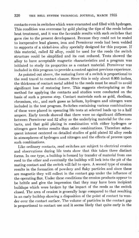
320 THE BELL SYSTEM TECHNICAL JOURNAL, MARCH 1955

contacts even in switches which were evacuated and filled with hydrogen. This condition was overcome by gold plating the tips of the reeds before heat treatment, and it was the favorable results with such switches that gave rise to the present development. Because they could not be sealed to inexpensive lead glasses, iron and Perminvar reeds had been welded to supports of a nickel-iron alloy specially designed for this purpose. If this material, called 52 alloy, could be used for the reeds the switch structure could be simplified and its cost reduced. Tests showed the alloy to have acceptable magnetic characteristics and a program was initiated to study its properties as a contact material. Perminvar was included in this program to provide a control against previous experience.

As pointed out above, the restoring force of a switch is proportional to the reed travel to contact closure. Since this is only about 0.005 inches, the thickness of contact metal added to the reeds must be small to avoid significant loss of restoring force. This suggests electroplating as the method for applying the contacts and studies were conducted on the basis of such a process step. Contact materials such as gold, rhodium, chromium, etc., and such gases as helium, hydrogen and nitrogen were included in the test program. Switches containing various combinations of these were placed in operating life tests at selected loads up to a half ampere. Early trends showed that there were no significant differences between Perminvar and 52 alloy as the underlying material for the con- tacts, and that gold plating in combination with either hydrogen or nitrogen gave better results than other combinations. Therefore subse- quent interest centered on detailed studies of gold plated 52 alloy reeds in atmospheres of hydrogen and nitrogen and the effects of process upon such combinations.

Like ordinary contacts, reed switches are subject to electrical erosion and observations during life tests show that this takes three distinct forms. In one type, a buildup is formed by transfer of material from one reed to the other and eventually the buildup will lock into the pit of the mating contact and the switch will fail to open. A second type of erosion results in the formation of powdery and flaky particles and since these are magnetic they will collect in the contact gap under the influence of the operating flux. Under these conditions the erosion products appear to be brittle and give the impression that they may have been incipient buildups which were broken by the impact of the reeds as the switch closed. The area of erosion is generally large compared to that resulting in an early buildup showing a disposition of the point of contact to wan- der over the contact surface. The volume of particles in the contact gap is proportional to contact use and it seems likely that quite early in the

DEVELOPMENT OF REED SWITCHES AND RELAYS 321

switch life, if no single predominant buildup has occurred, the electrical contact between the reeds is through these particles which are conduct- ing and are distributed over the contact area rather than by direct con- tact between the reed surfaces. While some of the particles may be welded to the reed surfaces most of them are loose and under the in- fluence of the gap flux become rearranged at each switch operation. This action may promote distribution of contact wear but can also lead to aggregations which can become welded together and initiate a predomi- nant buildup resulting in ultimate contact locking. It has also been observed that after many operations the volume of particles may become great enough so that their rearrangement will permit them to bridge the gap of the unoperated switch and thus cause contact failure or other malfunctioning. Obviously, this type of erosion is very complex and its consequences are difficult to predict. A third type of erosion occurs in a significant number of switches. Here a buildup takes the form of a puddle-like formation covering an appreciable part of the contact surface with a corresponding shallow depression in the mating contact. Contacts with this type of erosion have much less loose material than contacts of the second type but when they fail it is due to the relatively sudden appearance of a buildup causing locking.

Switches having only the first kind of erosion frequently exhibit short life and are rather uncommon. Those of the second kind are representa- tive of the present state of the art and account for the bulk of the failures observed. Switches having the third kind of erosion give an operating life about ten times as long as those having the second kind. The causes for these differences in contact erosion are not well understood but they appear early in the switch life. For this reason it is suspected that they may be related to such factors as the smoothness and alignment of the reed surfaces, the degree of penetration of the contact material into the underlying reed and process contaminants. These can all affect the reed surfaces and influence the nature of the initial erosion and thereby pos- sibly determine its course through the switch life. The large number of interrelated variables bearing on switch life makes it very difficult to obtain an evaluation through small scale laboratory experiments and there can be no assurance that the same factors will exist in the process for large scale manufacture. For this reason an important part of the continuing program for contact development will be the study of the output from regular manufacture and the effects of variations introduced in the process.

Operating life tests for reed switches have been conducted mostly at one-eighth and one-half ampere resistive or protected inductive loads.

322 THE BELL SYSTEM TECHNICAL JOURNAL, MARCH 1955

Tests of switches from the early stages of large scale manufacture show that a few of these failed as early as 200 million operations, about half had failed at one billion operations and some were still going at two billion operations. This large spread in the performance of supposedly identical switches does not appear related to the load conditions and therefore must be considered a switch attribute. It is thought that in part it must be due to the fortuitous nature of the second type of erosion described above since both it and the third type of erosion are found in the long life switches and there were no early failures having the third type. In evaluating the behavior of sealed switches it must be remem- bered that their contacts are not accessible for servicing and for this reason the first failure of a switch must be considered the end of its use- ful life. On this premise reed switch life in the load range from one eighth to one-half an ampere must be taken as about 200 million operations. For smaller loads longer life may be expected exceeding a billion opera- tions for very small loads. The capabilities discussed are all for 48-volt load circuit conditions.

DESIGN FOR MANUFACTURE

With this background of information it became possible to adopt a switch design and a manufacturing process which would permit a suffi- cient degree of mechanization to predict acceptable costs. In this design shown in Fig. 6 the reeds are made from 52 alloy wire in the shape of a double-ended paddle with a round section near its middle. The round section provides optimum conditions for minimizing stress concentra- tions in the metal-to-glass seal. One flat end of the paddle provides the moving reed inside of the switch and the other provides the external electrical connection. Both ends are gold plated, one to act as the elec-

"-"-H

GLASS TUBE

J c PLATED CONTACTS

COMPLETED SWITCH

Fig. 6 — Reed switch design suitable for large scale manufacture.

DEVELOPMENT OF REED SWITCHES AND RELAYS 323

trical contact and the other to provide for ease of soldering an external connection to the switch. The final design also had to avoid the use of metal tabulations if cost objectives were to be met, and the methods for pumping and filling used in the vacuum tube art were considered too expensive. Novel methods were explored. One of these was to enclose

e a

•>

Fig. 7 — Laboratory facility for the semiautomatic assembly and flush-filling of reed switches.

324 THE BELL SYSTEM TECHNICAL JOURNAL, MARCH 1955

the entire switch assembly machine in the atmosphere desired for switch filling. This method received considerable experimental study and it was concluded that the problems of switch cleanliness in the presence of machine lubricants and other contaminants would be difficult to solve. The means selected was to mount the reeds and the glass envelope in the proper position for sealing and then displace the air in the envelope by flushing with the desired gas. Extensive experiments were required to design means for introducing the gas so that aspirator effects would not draw in air during the flushing process and the whole technique of glass sealing had to be revised to allow for the cooling effects of the flowing gas as the seals were closing. Fig. 7 shows the laboratory setup for this development. The two heater coils are clearly visible and between them a clip for holding the glass tube. Above the upper heater is seen the chuck for holding the upper reed. At the bottom is the chuck for holding the lower reed and it provides the means for introducing the gas including a chamber for assuring its lamellar flow. It is mounted on a track and under control of a servo motor may be moved to obtain the desired switch gap. The upper chuck and the sealing heaters are mounted on vertical slides so that after the reeds and glass tube have been loaded the reeds can be inserted in the glass tube by operation of the levers shown. After this the machine operation is programmed by auxiliary facilities. The air is flushed from the glass tube while the servo establishes the desired switch gap. The upper heat coil is then energized and when this seal has been effected the velocity of gas flow is lowered and the lower seal is made. Aside from their value in supplying requirements for final machine design these automatic features were an absolute necessity in providing a sufficient degree of process stability to permit significant conclusions to be drawn from small lots of switches intended to display the effects of specific design or process changes.

II — Reed Relays

The combination of a reed switch and an operating coil constitutes a relay and in contrast to other relays no magnetic core, armature or con- tact carrying springs are required. The design of switch developed pro- vides a simple make contact. However, as will be described below, break and transfer functions and other worth while features can be obtained by associating a permanent magnet with a make contact reed switch.

RELAYS WITHOUT MAGNETS (NEUTRAL)

If a single switch is placed in an operating coil and the current through the coil is increased there will be a definite value of ampere turns at which

DEVELOPMENT OF REED SWITCHES AND RELAYS 325

OPERATE - OPERATE -

OPERATE -

NON-OPERATE - HOLD -

NON-OPERATE -

HOLD -

RELEASE -

RELEASE -

RELEASE -

STAFF 1 STAFF 2 STAFF 3

Fig. 8 — Comparison of the operating characteristics of a single reed relay with that of the relay type universe of which it is a sample.

the switch will close. When the current is then decreased, there will be another definite value at which the switch will open. These are called the operate and release values of that switch and are shown on Staff 1 of Fig. 8 where the ordinates are operating coil ampere turns. Sealed switches are not adjustable and their individual operating values are subject to manufacturing tolerances. In consequence, if a succession of switches are measured in the same operating coil the results are as indicated on Staff 2. As the coil current is increased from zero there will be an ampere turn value at which the most sensitive switch will just fail to close; this is called the non-operate value of that relay design and is the highest ampere turn value at which no relay will operate. As the ampere turn value is further increased a value will be found just sufficient to assure that all switches will close; this is called the operate value of the relay. If the coil current is then decreased, a value will be found below which one or more switches will open; this is called the hold value of the relay and the still lower point at which all switches will just have opened is called the release value of the relay. The difference between operate and non-operate and that between hold and release represent the manufacturing spread in the nominal operate and release values of a given relay design. These four characteristics are important to circuit designers and considerable development effort is justified to

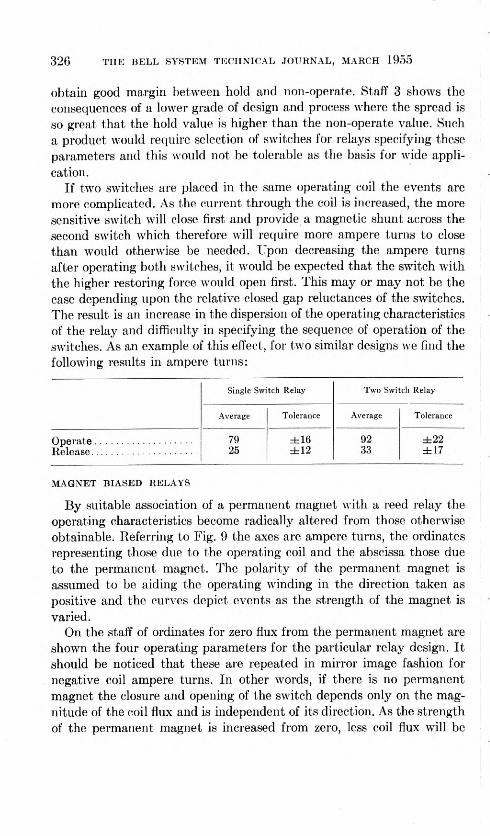
326 THE HELL SYSTEM TECHNICAL JOURNAL, MARCH 1955

obtain good margin between hold and non-operate. Staff 3 shows the consequences of a lower grade of design and process where the spread is so great that the hold value is higher than the non-operate value. Such a product would require selection of switches for relays specifying these parameters and this would not be tolerable as the basis for wide appli- cation.

If two switches are placed in the same operating coil the events are more complicated. As the current through the coil is increased, the more sensitive switch will close first and provide a magnetic shunt across the second switch which therefore will require more ampere turns to close than would otherwise be needed. Upon decreasing the ampere turns after operating both switches, it would be expected that the switch with the higher restoring force would open first. This may or may not be the case depending upon the relative closed gap reluctances of the switches. The result is an increase in the dispersion of the operating characteristics of the relay and difficulty in specifying the sequence of operation of the switches. As an example of this effect, for two similar designs we find the following results in ampere turns:

Single Switch Relay Two Switch Relay

Average Tolerance Average Tolerance

Operate Release

79 25

±16 ±12

92 33

±22 ±17

MAGNET BIASED RELAYS

By suitable association of a permanent magnet with a reed relay the operating characteristics become radically altered from those otherwise obtainable. Referring to Fig. 9 the axes are ampere turns, the ordinates representing those due to the operating coil and the abscissa those due to the permanent magnet. The polarity of the permanent magnet is assumed to be aiding the operating winding in the direction taken as positive and the curves depict events as the strength of the magnet is varied.

On the staff of ordmates for zero flux from the permanent magnet are shown the four operating parameters for the particular relay design. It should be noticed that these are repeated in mirror image fashion for negative coil ampere turns. In other words, if there is no permanent magnet the closure and opening of the switch depends only on the mag- nitude of the coil flux and is independent of its direction. As the strength of the permanent magnet is increased from zero, less coil flux will be

DEVELOPMENT OF REED SWITCHES AND RELAYS 327

needed to close the switch and the four relay parameters will behave as shown by the curves. To illustrate, if the magnet strength were 10 ampere turns the coil operate ampere turns would be reduced from 110 to 100 and the release ampere turns from 20 to 10 ampere turns. If negative coil flux were applied for this condition it would take 120 ampere turns to close the switch compared with 110 ampere turns for the case of no permanent magnet. Therefore, increasing the magnet strength increases the sensitivity of the relay and provides additional margin against opera- tion by unwanted negative current. As the strength is increased further a point will be reached where it is equal to the release value of the relay design. Beyond this point some of the relays will fail to release on coil open circuit. This limit, indicated by the dashed ordinate A gives the

125

100

75

50

26

z 5 0 h~ (U a HI 0.-25 2 <

-50

-75

-100

-126

-150 0 25 50 75 100 125 150

MAGNET AMPERE TURNS

Fig. — Typical operating characteristics of a magnet biased reed relay.

?/■

AT- >w-o

328 THE BELL SYSTEM TECHNICAL JOURNAL, MARCH 1955

useful range for magnet bias as a means for increasing relay sensitivity. In the operating range from 0 to A there is the additional possibility that by adjusting the magnet strength the spreads in the operate or release characteristics of the relay can be reduced. However, both of these values cannot be controlled simultaneously.

In the operating region between A and 13 some of the relays will release on coil open circuit and others not. This operating region would require selection of switches and is only useful for special applications.

PULSE OPERATION

The operating region between B and C is of great interest. Any relay in this region when operated will remain operated and will require re- versed coil current to be released. Due to the high speed of the switch, operation can be accomplished by pulses of a few milliseconds and no holding power will be required to keep the switch closed. Likewise the switch can be released by a negative pulse. In this region the switch can perform either the make or the break function as desired and the pulses may be symmetrical or assymmetrical in cither direction. This is also the most sensitive operating region of the relay.

NORMALLY CLOSED OR BREAK OPERATION

Further increases in the magnet bias in the region from C to D yields another region of uncertainty. Operation here would be with negative coil current which should cause the relay contacts to open but some re- lays would fail to reclose on open circuit.

The region beyond D is again generally useful and here the operation is that of a normally closed contact which opens on negative coil current. When the magnet strength becomes equal to the sum of the operate and release ampere turns of the switch design the relay is a break relay with the same sensitivity as a neutral make relay. The additional cost of a break relay will be that of the magnet and its adjustment.

TRANSFER RELAY

The transfer function can be performed by using a make and a break relay with simultaneous excitation of their windings and suitable con- nections to their switches.

RELAY DESIGN

The design of a relay includes a packaging problem. Heretofore this has been based upon using the relay core as a central stucture to which

DEVELOPMENT OF REED SWITCHES AND RELAYS 329

Fig. 10 — Models showing the construction of basic relay units. These may be used singly or in assemblies.

was attached the operating windings, armature, contact springs, covers and the means for mounting this assembly. Reed switch relays having no magnetic cores must use other means to provide a method for mounting.

In the case of reed switch relays a new design requirement arises from the needs of the maintenance personnel in the operating telephone plant. Over the years, maintenance personnel tracing circuit troubles have been aided by visually determining the state of operation of relays and other electromechanical devices. Additionally, by having access to the contacts they could as desired isolate portions of circuits by "toothpicking" in- dividual contacts to cause them to remain open or closed regardless of the operating state of the relay. Because the reed switch magnetic gap and contacts arc inside of the operating coil neither of these well estab- lished techniques can be used and the relay designer must provide other means for maintenance.

One design approach to the reed relay rests upon the concept of a basic building block composed of a coil containing 1, 2, 4, 6 or 10 switches. The inside dimensions of the coil and its shape conforms to the number of switches to be used and applications requring an odd number of switches can use the next higher even sized building block. Fig. 10 shows two of these basic units, one for a single switch, the other for two. Shown in the picture are the terminals which take the form of metal strips projecting beyond the switch ends. These terminals arc held in position on the outside of the coil by acetate spoolheads and locked by acetate sheeting. Each terminal is shaped to provide means for making connec-

330 THE BELL SYSTEM TECHNICAL JOURNAL, MARCH 1955

tion to switches and coil leads. One end of each terminal is also shaped to accept machine wrapped connections to the external circuit while the other end can serve as electrical access for test purposes. In the single switch unit shown all of the connections to the coil and switch were needed in the circuit so four terminals were provided. In the two switch unit one of the switches is to be used for locking purposes so that only five external connections were needed.

These basic units may be used singly or in combinations. For each specific design simple molded parts are provided which slip over the ter- minal strips of the desired number and kind of subassemblies and lock them together. The resulting assembly is then surrounded by a shield of magnetic material to reduce interference to or from other electromag- netic apparatus. This assembly is then slipped into a case which provides the means for mounting the whole. Here again new design principles have been applied as seen in Fig. 11. The four corners of the case are extended and provided with detents and the case is suitably slit to con- trol the compliance of the corners. To mount this assembly it is simply pushed into suitable holes in a mounting plate. After passing through the holes the detents lock the assembly into position. This method of mounting eliminates the need for mounting screws and the space they would occupy and permits the fullest realization of the inherent compact-

Fig. 11 — A digit register which is an assembly of five relay units each contain- ing two reed switches. A digit is stored by operating two of the relays on the basis of a 2 out of 5 code.

DEVELOPMENT OF HEED SWITCHES AND RELAVS 331

6

5

i/) Q

LU •A -I - 3 2 Z

l-

1

0 3 4 6 8 10 20 40 60 100 200 6 6 10 20 40 60 100

N2/R IN KILOMHOS

Fig. 12 — Operating speed of typical reed relays versus operating coil design constant N2/R.*

ness of reed relays. Fig. 11 shows the details of an assembly of five relays each containing two switches. This is a digit register for use in storing a digit by the operation of two of the five relays. This register occupies about three square inches of panel space and performs the same func- tions as five standard relays requiring about ten square inches of space. It appears possible to plan the building blocks so that the height of relay assemblies will permit two rows on a standard 2" mounting plate. By spreading the relays in two rows the resulting presentation of terminals avoids wiring congestion. The wiring terminals of the relay are at the mounting end while the test terminals are at the free end. This gives access to the relay test points from the equipment aisles and testing from the wiring sides of frames is avoided. By molding grooves in the end insulators and providing soldering lugs on the terminals means for strapping between coils and switches is made possible inside of the relay assembly at less cost than could be done in the course of equipment wir- ing. Wiring straps can be seen in the illustration and these further reduce wiring congestion on the equipment frames.

The operating speed versus relay coil design constant is shown for various circuit power inputs in Fig. 12 for one and two switch relays of the basic design described above. These characteristics compare very

* M. A. Logan, Estimation anil Control of the Operate Time of Relays, B.S.T.J., 33 pp. 144-186, Jan., 1954.

TWO-SWITCH RELAY

ONE-SWITCH RELAY

2.5

0.075 WATT 2.0

V 0.46 0.10 1,5 WATTS

0.77 0.15 1.15

1.33 0.3 2.30 3,30 0,6 4.61 0,5 I .0 2.0

I

332 THE BELL SYSTEM TECHNICAL JOURNAL, MARCH 1955

favorably with those of other types of relays now used in the telephone plant.

At this writing a number of relays and relay assemblies have been de- signed for use with reed switches and several are already in manufacture by the Western Electric Company which is also producing the reed switches. All of these are of the neutral type without permanent magnet bias. Applications of these relays are conservative and are made in cir- cuits where the contacts make or break only moderate loads. Further development of the contacts, coupled with field experince will permit gradual broadening of use but even so millions of these switches will be required during the next few years.

ACKNOWLDEGMENT

The authors wish to acknowledge their indebtedness to members of the Materials, Chemical and Research Departments of Bell Telephone Laboratories for assistance with special problems. Mention should also be made of our associates in the Switching Apparatus Development De- partment, particularly Dr. W. B. Ellwood who originated the reed switch and carried out its early development as well as N. Insley and N. J. Velardi who jointly contributed the bulk of the design and process development for manufacture.

Stability of Negative Impedance Elements

in Short Transmission Lines

By J. GAMMIE and J. L. MERRILL, JR.

(Manuscript received November 29, 1954)

Until recently, voice frequency repeaters of the two-way type have been applied almost exclusively to electrically long transmission lines. Now, nega- tive impedance repeaters are used in quantity in the exchange telephone plant, and applications to electrically short lines arise more frequently. Because lower over-all transmission losses can be obtained by utilizing the lower phase shift in short lines, a different engineering approach to the application of E-lype negative impedance repeaters is desirable.

This paper outlines a general method whereby transmission performance and stability can be related to the characteristics of a symmetrical repealer located in the center of a short transmission line. The theory is particularly applicable to negative impedance repeaters. A tandem arrangement of short sections of transmission line, where each section has a centrally located re- peater, can be classed as a line loaded with negative impedance.

1. INTRODUCTION

For a period of about 40 years voice frequency repeaters have been engineered to provide amplification for both directions of conversation in two-wire telephone lines. Some of these repeaters have been operated in lines over 50 miles long; others have been operated in lines shorter than 10 miles. Yet practically all, including negative impedance repeaters of the E-type1, have been associated with transmission lines which can be classed as electrically long in that they have exceeded one half wave- length at the highest frequency in the pass-band.

Within the past few years the need for two-way amplification in elec- trically short lines in the exchange area plant has become increasingly evident. A short section of line has limited phase shift at voice frequen- cies, and advantage can be taken of this fact in the repeater design, to reduce the over-all attenuation below that obtainable with design

333

334 THE BELL SYSTEM TECHNICAL JOURNAL, MARCH 1955

methods applicable to electrically long lines. Furthermore, the use of negative impedance devices such as E-type repeaters has made it possible to consider engineering the repeater as an integral part of an electrically short line. This method of design is a logical one because in addition to the reduction in over-all attenuation, the image impedances seen looking into the line terminals are modified by the addition of the repeater. In effect, the philosophy of the hybrid coil and the 22-type repeater is discarded along with the idea that the image impedance of the repeater must match the characteristic impedance of the line. Where the repeater is located a distance less than one quarter wavelength (at a frequency of 4,000 eps) from either line terminal, better transmission performance generally can be obtained by a mismatch between the image impedance of the repeater and the characteristic impedance of the line.

Once a change in philosophy in matching the repeater to the line im- pedance is made, it becomes easier to forget the repeater as a separate device and to treat it as an integral part of the line in the way a loading coil would be treated. Hence, interest is centered upon the propagation constant and image impedances of the repeatered or loaded line and the transmission characteristics of the device itself are subordinated to this end.

When a two-wire repeater, or its equivalent in the form of a network of active elements, is inserted in a transmission line, stability (freedom from oscillation) becomes a prime consideration. In electrically short lines, the image impedance as well as the loss of the over-all line is a function of the degree of stability desired, which in turn will depend upon the requirements of the system in which the repeatered line must op- erate.

It is the purpose of this paper to relate transmission characteristics with stability, for a repeater in the form of a symmetrical active network located in the center of an electrically short transmission line. The equa- tions shown and the method of solution are particularly applicable to the fundamental design of E-type negative impedance repeaters in trans- mission lines wherein the repeater is located less than a quarter wave- length from the line terminals. The frequency at which this wavelength is determined is the highest desired in the pass-band.

The problem is attacked by taking the general case of the symmetrical two-wire repeater located in the center of a transmission line as shown in Fig. 1 (a) and substituting for the repeater the equivalent lattice shown in Fig. 1(b). This lattice consists of series arms, ZA/2, and shunt arms, 2Zb ■ The method described herein is general and can be applied to any

STABILITY OF NEGATIVE IMPEDANCE ELEMENTS 335

type of impedance in either the series or the shunt arm. However, be cause the specific application considered here is for the E'-type repeater, 7jA is specified as an open circuit stable negative impedance and Zb is specified as a short circuit stable negative impedance. This is designated on Fig. 1(b) where these impedances are defined as the ratio of two polynominals which are functions of the complex frequency variable p. It is understood that these impedances will have negative resistance components at some real frequencies because the term negative im- pedance is used herein to describe an impedance whose resistive com- ponent is negative within some band of frequencies.

Three conditions are considered: (a) An El or E2 repeater of negative impedance ZA in series with the

line (special case where Zb is infinite). (b) An E3 repeater of negative impedance Zb shunted across the line

(special case where ZA is zero). (c) The E23 repeater in the line (case of Fig. 1(b), which is the lattice

equivalent of the bridged T arrangement of the E23 repeater).

l/z OF

PHYSICAL LINE

SYMMETRICAL TWO-WIRE REPEATER

l/z OF PHYSICAL LINE

1 "2 >Za lit Zb<

(a) Zh = IMAGE IMPEDANCE OF LINE + REPEATER Pi = PROPAGATION CONSTANT OF LINE + REPEATER

ACTIVE NETWORK /2

/v\ l/z OF

PHYSICAL LINE

t/Z ZZ 2 Z OF PHYSICAL

LINE

(b)

Z NUp) WHERE Qjpj HAS NO ZER0S ,N THE D(p) RIGHT HALF p-PLANE

1 - WHERE M(p) HAS NO ZEROS IN THE B(p) RIGHT HALF p-PLANE

Fig. 1 —Symmetrical two-wire repeater in transmission line, (a) Schematic, (b) Kquivalent circuit.

330 THE BELL SYSTEM TECHNICAL JOURNAL, MARCH 1955

2. GENERAL STABILITY CRITERIA

Before the specific objective is considered, stability criteria will be reviewed briefly and a stability theorem applicable to symmetrical linear four-pole networks will be described.

2.1. Basic Stability Equation

The stability of the network of Fig. 1(a) can be determined from an examination of the roots in the complex frequency plane of the equation:

The quantity on the left hand side of the equation is the reciprocal of the interaction factor2 and its use as a measure of stability has been discussed by F. B. Llewellyn.3

As pointed out by Llewellyn Eq. (1) bears a striking similarity to the famous Nyquist equation for stability of feedback amplifiers, usually written

In both cases the fundamental requirement for stability is that the equa- tions should have no roots in the right half complex frequency plane.

In specific cases, the Nyquist criterion for stability can be applied by plotting on the complex plane as a function of real frequency the factors in (1) which correspond to ju/S, and seeing whether the plot encircles the point (1, jO).

In general, however, the fact that the point (1, jO) is outside such a plot is not in itself proof of stability. This ambiguity in the interpreta- tion of the diagram can be resolved if the factors involved in (1) are evaluated at complex frequencies.

It should be noted that a separate plot at real frequencies would be required for each combination of terminating impedance Zn and Zb. The assumption of particular values for Za and Zb would naturally lead to specialized stability criteria and it was to avoid this that Llewellyn

(1)

where:

Zh = Image impedance of the over-all line

PC = Propagation constant of the over-all line

Za = Impedance of one line termination

Zb — Impedance of the other termination

(1 - M/3) = 0

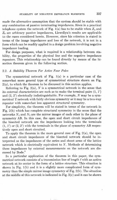
STABILITY OF NEGATIVE IMPEDANCE ELEMENTS 337

made the alternative assumption that the system should be stable with any combination of passive terminating impedances. Since in a practical telephone system the network of Fig. 1(a) has to be stable when Za and Zh are arbitrary passive impedances, Llewellyn's results are applicable to the cases considered herein. However, since his criterion is stated in terms of the image impedances and loss of the network, it is not in a form which can be readily applied in a design problem involving negative impedance loading.

For design purposes, what is required is a relationship between sta- bility, the properties of the physical line and the negative impedance repeaters. This relationship can be found directly by means of the bi- section theorem given in the following section.

2.2. A Stability Theorem For Active Four Poles

The symmetrical network of Fig. 1(a) is a particular case of the somewhat more general type of symmetrical structure shown on Fig. 2(a), to which the theorem to be discussed in this section applies.

Referring to Fig. 2(a), iV is a symmetrical network in the sense that its external characteristics are such as to make the terminal pairs (1, 1') and (2, 2') electrically indistinguishable. For example, N may be a sym- metrical T network with fairly obvious symmetry or it may be a two-way repeater with somewhat loss apparent structural symmetry.

For simplicity, the theorem will be stated in terms of the network in Fig. 2(b) which has complete structural symmetry in the sense that the networks AL and N-i are the mirror images of each other in the plane of symmetry AB. In this case, the open and short circuit impedances of the bisected network are the impedances looking into the terminals (1, 1') or (2, 2') with the terminals in the plane of symmetry AB respec- tively open and short circuited.

To apply the theorem in the more general case of Fig. 2(a), the open and short circuit impedances of the bisected network should be in- terpreted as the impedances of the series and shunt arms of the lattice network which is electrically equivalent to N. Methods of determining these impedances by external measurements on the network are dis- cussed by Bode.4

In a particular application of the theorem in this paper, the sym- metrical network consists of a transmission line of length f with an active network at its center in the form of a lattice structure. This situation is shown in Fig. 1(b) and it is a slightly more complicated form of sym- metry than the simple mirror image symmetry of Fig. 2(b). The situation at the middle of this network is indicated in Fig. 2(c) and it can be shown

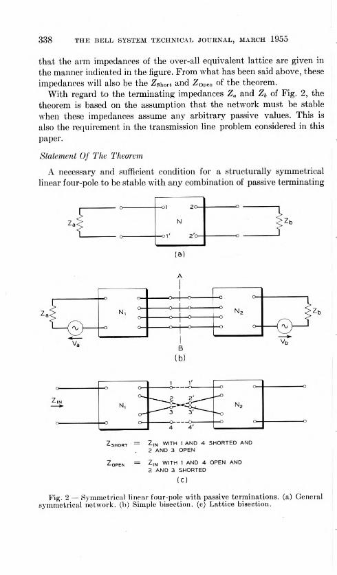
338 THE BELL SYSTEM TECHNICAL JOURNAL, MARCH 1955

that the arm impedances of the over-all equivalent lattice are given in the manner indicated in the figure. From what has been said above, these impedances will also be the Zshort and ZopeD of the theorem.

With regard to the terminating impedances Za and Zi, of Fig. 2, the theorem is based on the assumption that the network must be stable when these impedances assume any arbitrary passive values. This is also the requirement in the transmission line problem considered in this paper.

Statement Of The Theorem

A necessary and sufficient condition for a structurally symmetrical linear four-pole to be stable with any combination of passive terminating

Ol 20

Zb

ol' 20

B (b)

ZsmORT

Zqpen

Z|N WITH 1 AND 4 SHORTED AND 2 AND 3 OPEN Z|N WITH 1 AND 4 OPEN AND 2 AND 3 SHORTED

Fig. 2 — Symmetrical linear four-pole with passive terminations, (a) General symmetrical network, (b) Simple bisection, (c) Lattice bisection.

STABILITY OF NEGATIVE IMPEDANCE ELEMENTS 339

impedances is that the open and short circuit impedances of the bisected network shall he positive real impedance functions. These open and short circuit impedances are the input impedances of either half of (he network when the terminals in the plane of bisection arc respectively open and short circuited. The term passive impedance as used herein denotes a positive real impedance function.

The theorem is proved in Appendix A and therein also arc found the requirements for an impedance function to be positive real.

3. SERIES NEGATIVE IMPEDANCE LOADING

This is the case of Fig. 1(b) where Zb is infinite and where ZA is a nega- tive impedance of the open circuit stable type. It also represents the installation of an El or E2 repeater in the center of an electrically short transmission line.

3.1. Stability

Consider Fig. 3(a) where a negative impedance of the open circuit stable type {ZA) is shown in the center of a physical transmission line. The problem is to determine the equations which relate transmission characteristics with stability for all passive terminating impedances.

According to the bisection theorem stated in 2.2 the network of Fig. 3(a) will be stable for all passive impedance terminations provided the open and short circuit impedances of the bisected network are positive real. The short circuit impedance of the bisected network is shown in Fig. 3(b) and is represented by Z„ multiplied by Tanh Pf/2. This must be made positive real. The open circuit impedance of the bisected net- work is shown in Fig. 3(c) and is expressed as Z,{ divided by Tanh PC/2. This open circuit impedance is positive real because it equals the open circuit impedance of one half of the physical line, Zor . Thus it has no direct bearing on stability but does contribute the relationship:

= — y CoN Tanh P//2 Tanh ^1/2 JOC y '

where:

Zh = Image impedance of the line with ZA

PC = Propagation constant of the line with ZA

Zo = Characteristic impedance of the physical line

^ = Propagation constant of length C of physical line

340 THE BELL SYSTEM TECHNICAL JOURNAL, MARCH 1955

l/Z OF PHYSICAL

LINE

Za -wv

(6)

l/z OF PHYSICAL

LINE

ZH TANh VL/z

Za/2 vw-

OF SHORT PHYSICAL

LINE

Za/2 VW

TANh P^/2 OPEN OF PHYSICAL

LINE

ZH TANh PL/z — ZqC 1/K/Z + Zsc

ZA/H + Zoc

(b)

TANh Pi/2 TANh 7 l/z

(C)

= Zr

where: Zh P t Zo y Zoc Zsc

= Image impedance of physical line with ZA = Propagation constant per unit length — line with = Length of physical line = Characteristic impedance of physical line = Propagation constant per unit length of physical line

Zp Tanh yC/2

= Zo Tanh y(/2. Fig. 3 — Application of bisection theorem to series loading, (a) Schematic,

(b) Short circuit impedance of bisected network, (c) Open circuit impedance of bisected network.

Equation (2) demonstrates an important relationship which has been known ever since the discovery of coil loading. It is worthwhile repeating here because the network in Fig. 3(a) is, in fact, a single section of line loaded with a series impedance ZA . Equation (2) demonstrates that the midsection impedance and propagation constant of the loaded line bear the same relationship to each other as the corresponding parameters of the nonloaded line bear to each other. Thus the general relationship be- tween propagation constant and midsection impedance of a loaded line is to this extent independent of the loading element.

With regard to stability, the application of the bisection theorem to Fig. 3(a) has shown that the basic criterion for stability is that Zn

Tanh PC/2 must be a positive real impedance function. This impedance can be expressed in terms of physical line parameters and ZA as follows:

Z,, Tanh PC/2 = Zo Tanh {M + yC/2) (3)

STABILITY OF NEGATIVE IMPEDANCE ELEMENTS 341

where

M = Tanh"1 ^ AfJO

Zq = Characteristic impedance of the physical line

There are two requirements which must he placed upon Zq Tanh {M + yt/2) for it to be positive real. One of them is that in the following equation, R shall be a positive resistance at all frequencies.

Z0 Tanh {M + yt/2) = R± jX (4)

The other requirement will be reserved until (4) has been discussed. The limit of stability will be approached as R approaches zero. If

(4) is taken to the limit of stability then:

Zo Tanh (M + yC/2) = ±jX (5)

where as before

M = Tanh- ^

If at a single frequency all values of Za/I which satisfy (5) are plotted on the Z-plane, their locus will trace a circle because jX is a straight line and the relationship is a bilinear transformation.5 Formulas for the centers and radii of these circles are given in Appendix B. If, as is the case with telephone cable, the characteristic impedance Zo has a negative angle, this trace will appear as shown in Fig. 4. The region inside this

I. '/// REGION \ V^Xnstability A/T

R 0 +

Fig. 4 — Circle for determining the stability of a loading element in a line.

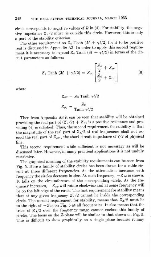
342 THE BELL SYSTEM TECHNICAL JOURNAL, MARCH 1955

circle corresponds to negative values of R in (4). For stability, the nega- tive impedance Z^/2 must lie outside this circle. However, this is only a part of the stability criterion.

The other requirement on Zo Tanh (il/ + y(/2) for it to be positive real is discussed in Appendix A3. In order to apply this second require- ment it is necessary to expand Zo Tanh (il/ + yt/2) in terms of the cir- cuit parameters as follows:

Z0 Tanh {M + y(/2) = Z0c

Za A- 7 T + Zsc

Z* y 7 2" + Zoc

(6)

where

ZSc = Zo Tanh yC/2

7 - Zo Aoc — Tanh yf/2

Then from Appendix A3 it can be seen that stability will be obtained providing the real part of (Z.,,/2) + Zsc is a positive resistance and pro- viding (4) is satisfied. Thus, the second requirement for stability is that the magnitude of the real part of Z.,/2 at real frequencies shall not ex- ceed the real part of Zsc , the short circuit impedance of f/2 of physical line.

This second requirement while sufficient is not necessary as will be discussed later. However, in many practical applications it is not unduly restrictive.

The graphical meaning of the stability requirements can be seen from Fig. 5. Here a family of stability circles has been drawn for a cable cir- cuit at three different frequencies. As the attenuation increases with frequency the circles decrease in size. At each frequency, —Zsc is shown. It falls on the circumference of the corresponding circle. As the fre- quency increases, —Zsc will rotate clockwise and at some frequency will be on the left edge of the circle. The first requirement for stability means that at any given frequency ZAI2 cannot lie inside the corresponding circle. The second requirement for stability, means that ZA/2 must lie to the right of —Zac on Fig. 5 at all frequencies. It also means that the trace of Z.4/2 over the frequency range cannot enclose this family of circles. The locus on the Z-plane will be similar to that shown on Fig. 5. This is difficult to show graphically on a single plane because it may

STABILITY UF NEGATIVE IMPEDANCE ELEMENTS 343

+

jx

o

f,<f2<f3 f'' \

\ VZ^C

\ ZA V 2 „

Fig. 5 — Stability circles for Z.i/2.

appear that the trace of Z,t/2 does go through the family of circles. However, where it apparently passes through the family of circles it does so at a lower frequency. At no given frequency does the trace of Z..,/2 lie within its stability circle.

The second requirement for stability, namely that the real part of (Za/2) + Zsc should be positive, is a sufficient condition but not a necessary one. A necessary and sufficient condition, when Za/2 is open circuit stable, is derived in Appendix A3. With reference to Fig. 5 this condition requires that the plot of Za/2 will not enclose any of the stabil- ity circles.

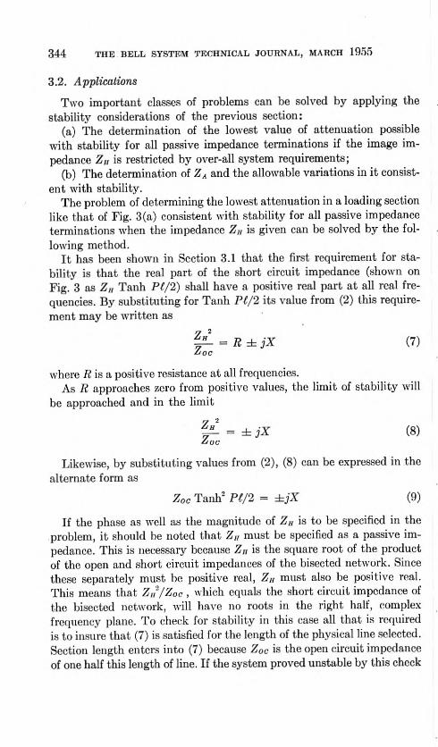
344 THE BELL SYSTEM TECHNICAL JOURNAL, MARCH 1955

3.2. Applications

Two important classes of problems can be solved by applying the stability considerations of the previous section:

(a) The determination of the lowest value of attenuation possible with stability for all passive impedance terminations if the image im- pedance Z,r is restricted by over-all system requirements;

(b) The determination of ZA and the allowable variations in it consist- ent with stability.

The problem of determining the lowest attenuation in a loading section like that of Fig. 3(a) consistent with stability for all passive impedance terminations when the impedance Zh is given can be solved by the fol- lowing method.

It has been shown in Section 3.1 that the first requirement for sta- bility is that the real part of the short circuit impedance (shown on Fig. 3 as ZH Tanh Pf/2) shall have a positive real part at all real fre- quencies. By substituting for Tanh Pt/2 its value from (2) this require- ment may be written as

= K ± jX (7) Aoc

where R is a positive resistance at all frequencies. As R approaches zero from positive values, the limit of stability will

be approached and in the limit

= ± jX (8) Aoc

Likewise, by substituting values from (2), (8) can be expressed in the alternate form as

Z0c Tanh2 PC/2 = ±jX (9)

If the phase as well as the magnitude of Zw is to be specified in the problem, it should be noted that Z„ must be specified as a passive im- pedance. This is necessary because Z„ is the square root of the product of the open and short circuit impedances of the bisected network. Since these separately must be positive real, Z,, must also be positive real. This means that ZH

2/Zoc , which equals the short circuit impedance of the bisected network, will have no roots in the right half, complex frequency plane. To check for stability in this case all that is required is to insure that (7) is satisfied for the length of the physical line selected. Section length enters into (7) because Zoc is the open circuit impedance of one half this length of line. If the system proved unstable by this check

STABILITY OF NEGATIVE IMPEDANCE ELEMENTS 345

the only recourse would he to solve for a section length which would prove stable.

If the magnitude only of Zw had been fixed then for each section length there would be a choice of phase angle for Zu within the limits prescribed by system requirements. For solution in this case (8) could be inter- preted to mean that for stability

7 2

the angle of < 90 degrees (10) Zoc

Eq. (2) can be rearranged as follows:

Tanh Pt/2 = ^ (11) Zoc

From (10) and (11) it may be shown that when the magnitude of Z,, is fixed, the closer the loading section is brought to instability by adjust- ing the angle of ZH , the lower will be the attenuation of the section. Thus this angle should be adjusted for minimum stability.

When the limit of stability is reached, (8) indicates that Z//'/Zoc will be a pure reactance but the question arises as to whether the angle of ZH should be adjusted to make the sign of the reactance positive or negative. The choice here is based on two observations. First, that if the angle of Zoc is negative, as it generally is for cable circuits, minimum over- all attenuation will result when the reactance on the right hand side of (8) is positive. Second, from (G) it may be shown that if the short circuit impedance of the bisected network is a positive reactance, Za/I will lie on the circumference of the stability circles of Fig. 5 on the arc to the right of — Zsc . In the case of lines such as are under consideration here, where the top frequency in the pass band is less than one quarter wave length, the second stability requirement which is discussed in Section 3.1 thereby will be satisfied within the pass band of frequencies.

Therefore, when the magnitude alone of Z,, has been specified the de- sign procedure is to select an angle for Z/, such that the angle of Z/r/Zoc is just less than +90 degrees. In (8), Zu/Zoc then will be nearly equal to ++Y and the magnitude of X will be given by the ratio of the magni- tude of Zu to the magnitude of Zoc . The magnitude and angle of Z,, now is determined for any chosen frequency in the band and the value of the negative impedance Z.,/2 required to give the desired value of ZH

can be obtained from the equation:

Z. = 2Zoc #+14 (12) Zr;/" Zoc"

where Zo is the characteristic impedance of the nonloaded line.

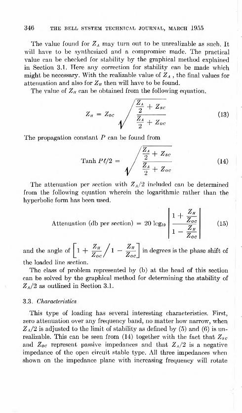
346 THE BELL SYSTEM TECHNICAL JOURNAL, MARCH 1955

The value found for 7jA may turn out to be unrealizable as such. It will have to be synthesized and a compromise made. The practical value can be checked for stability by the graphical method explained in Section 3.1. Here any correction for stability can be made which might be necessary. With the realizable value of ZA , the final values for attenuation and also for Zu then will have to be found.

The value of ZH can be obtained from the following equation.

Zh = Zc

The propagation constant P can be found from

Z, — + Z so

^ + z oc (13)

Tanh Ft/I = T + Zac

/ T

(14) + Z.

The attenuation per section with ZA/'l included can be determined from the following equation wherein the logarithmic rather than the hyperbolic form has been used.

Attenuation (db per section) = 20 logio 1 +

Zh_ Zoo

1 - z„

(15)

and the angle of 1 + [■+£/

1 - Z//

in degrees is the phase shift of Zoc/ Zoc.

the loaded line section. The class of problem represented by (b) at the head of this section

can be solved by the graphical method for determining the stability of Z,i/2 as outlined in Section 3.1.

3.3. Characteristics

This type of loading has several interesting characteristics. First, zero attenuation over any frequency band, no matter how narrow, when Z,,i/2 is adjusted to the limit of stability as defined by (5) and (6) is un- realizable. This can be seen from (14) together with the fact that Zsc and Zoc represent passive impedances and that Z,1/2 is a negative impedance of the open circuit stable type. All three impedances when shown on the impedance plane with increasing frequency will rotate

STABILITY OF NEGATIVE IMPEDANCE ELEMENTS 347

in the clockwise direction. For stability, the locus of Z.-)/2 must not enclose either —Zac or — Zon . At the limit of stability, however, Z^/2 must lie on the circles of stability which are shown on Fig. 5. This means a changing relationship between these three impedances with frequency which is incompatible with zero attenuation over any frequency band. Second, a flat response can be realized over a band of frequencies, in general, only at the expense of increasing the loss at the lower frequencies above that required for stability. Third, as the length of the physical line is increased, it becomes more and more difficult to obtain a low over- all loss and yet avoid the enclosure of the stability circles of Fig. 5 with a realizable design of Z,i/2. The practical limit here appears to be one quarter wave length of physical line at the highest frequency it is desired to pass.

4. SHUNT NEGATIVE IMPEDANCE LOADING

This case where ZB is shunted across the line conductors at the mid- point of a physical line (Fig. 1 (b) where ZA is zero) can be classed as shunt type negative impedance loading. The negative impedance Zb is of the short circuit stable type such as the impedance produced by the E3 re- peater. Hence, this case can represent an E3 repeater bridged across the conductors of an electrically short transmission line.

i/2 OF

PHYSICAL LINE

H i/2 OF

PHYSICAL LINE

>ZB

f

(a)

TANh P V2 t Z SHORT

Zh TANh Pi/2 = Zsc

(b)

i TANh Pi/? 2 Z

TANh Pi/2 ZoC

(0

2ZB + zsc 2 ZR +Znr

Fig. 6 — Application of bisection theorem to shunt loading, (a) Schematic, (b) Short circuit impedance of bisected network, (c) Open circuit impedance of bisected network.

348 THE BELL SYSTEM TECHNICAL JOURNAL, MARCH 1955

4.1. The Stability Equations

The same method described in detail in Section 3.1 is used here to determine stability. The short and open circuit impedances of the bisected network are obtained as shown in Fig. (i.

As seen from Fig. 6(b) the short circuit impedance of the bisected network is positive real being equal to Zsc , the short circuit impedance of the physical line of length f/2 .

ZH Tanh PC/2 = Zo Tanh yC/2 = Zsc (16)

The open circuit impedance of the bisected network [Fig. 6(c)] deter- mines stability. Thus for stability:

Z " must be a positive real impedance function.

Tanh PC/2 A substitution from (16) for Tanh PC/2 above will yield the following

requirement for stability:

^- = R±iX (17) ^sc

where R must be a positive resistance and Z,i a positive real impedance function.

The limit of stability is reached as R goes to zero. Therefore, the limit of stability for all passive impedance terminations can be expressed by:

= ±jX (18) ^SC

A similar equation can be obtained in terms of Tanh PC/2 rather than ZH .

Zsc Tanh2 PC/2

= ± jX (19)

4.2. Analysis

From Eq. (18) the sole criterion for stability is that the angle of

~ < 90° (20) Zsc

provided that ZH is a positive real impedance function. The value of the propagation constant can be found from (16) to be:

Tanh PC/2 = ^ (21) Z a

STABILITY OF NEGATIVE IMPEDANCE ELEMENTS 349

and from the short circuit and open circuit impedances, Fig. 6(b) and Fig. G(c), the following are found

vISErS (221

and

z- ■ ■/WlS] ""

In order to translate stability into engineering parameters, the open circuit impedance, Zw/Tanh Pf/2, can be expressed in parameters of the physical line and Zi, .

ZH

Tanh PC/2 = Z oc

[Srt;] «

By reasoning similar to that used in Appendix A and in Section 3.1 it can be shown that the requirement for stability will be met if

Re (--^r + ) is positive (25) \ZZb Zoc/

where ZH is a negative impedance of the short circuit stable type and pro- viding

+ Zac y \2ZB

4" Zoc_ = R ± jX (26)

where R is a positive resistance at all frequencies. The limit of stability will be reached as R approaches zero. If at any given frequency all values of 2ZU , which fulfill (26) when R

is zero, arc plotted on the Z-plane they will trace out the same circle as found before in Section 3.1 where ZA was likewise examined (if the fre- quency and physical line parameters arc the same in both cases). Thus 2ZB should not lie inside the stability circle of Fig. 4.

However, in order to meet the restriction imposed by (25) upon ZB , the locus of 2Zb when plotted over the frequency range from zero to infinity must enclose this family of circles as shown in Fig. 7. This can be established in much the same way as in Section 3.1 where it was proved that the locus of Z.4/2 must not enclose this family of circles.

Here, in the case of shunt loading, as in the case of series loading, zero attenuation is inconsistent with stability for all passive impedance ter- minations. Likewise, with shunt loading designed for minimum stability over the pass band the attenuation will vary with frequency.

350 THE BELL SYSTEM TECHNICAL JOURNAL, MARCH 1955

W 2Z

/ f.s cc

-z oc

zoc

0 +

Fig. 7 — Stability circles for 2Zn .

5. LATTICE LOADING

The general case of Fig. 1(b) is where the combination of an E2 and an E3 repeater is located in the center of an electrically short line. Al- though the actual E23 repeater is connected as a bridged T arrangement1

the equivalent lattice form is used herein for simplicity in explanation. What is said as applied to the lattice structure applies also to the bridged T.

Fig. 8(a) shows a lattice network of negative impedances connected at the midpoint of a line of length (. Negative impedance Za is open cir- cuit stable; ZB is short circuit stable.

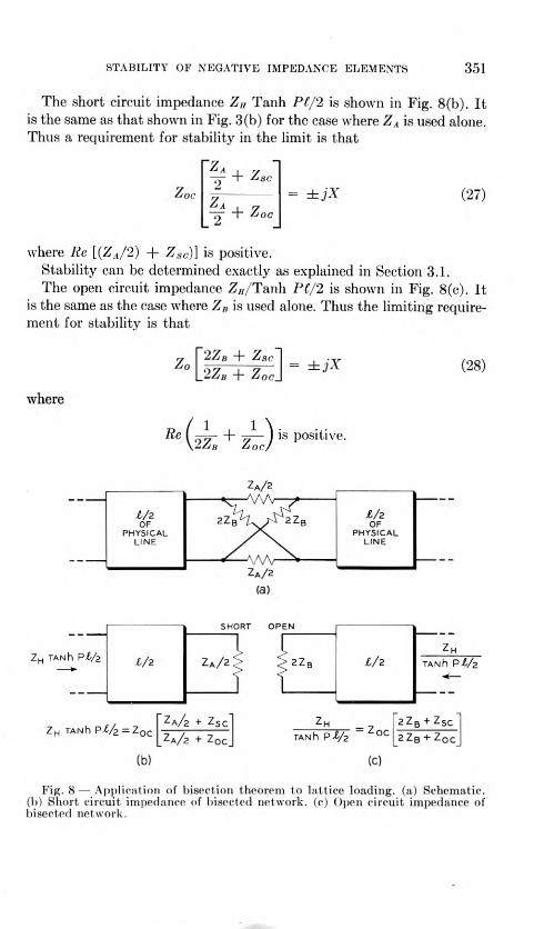
STABILITY OF NEGATIVE IMPEDANCE ELEMENTS 351

The short circuit impedance Z„ Tanh Pf/2 is shown in Fig. 8(b). It is the same as that shown in Fig. 3(b) for the case where ZA is used alone. Thus a requirement for stability in the limit is that

Zc

I 7 —y w

^4-7 2

+ Zoc

= (27)

where Re [(ZA/2) + Zac)] is positive. Stability can be determined exactly as explained in Section 3.1. The open circuit impedance 7,,/Tanh P(/2 is shown in Fig. 8(c). It

is the same as the case where Z,, is used alone. Thus the limiting require- ment for stability is that

y P27b d- Z3c~\ J0 \_2Zb + ZocJ = ±jX (28)

where

Re Gz.+ z„}

is positive.

1/2 OF

PHYSICAL LINE

\ 2Zb /

Za/2 V\A

1/2 2 Z OF PHYSICAL LINE

A/V Za/2

(a)

ZM TANh Pl/z

ZH TANh Pt/z = Zoc

(b)

i/2 Za/2

SHORT OPEN

Za/s + ZSc Za/2 + Zoc

1/2 TANh Pl/z 2Z

TANh Pi/s = 2. 2 ZR + Z< 2 ZB + Z(

(C)

Fig. 8 — Application of bisection theorem to lattice loading, (a) Schematic. (1>) Short circuit impedance of bisected network, (c) Open circuit impedance of bisected network.

352 THE BELL SYSTEM TECHNICAL JOURNAL, MARCH 1955

Stability can be determined as explained in Section 4.2 for (26). Thus stability with ZA is determined independently of ZB and the

converse is true also. In regard to stability each negative impedance can be designed without considering the other. The image impedance, ZH , and propagation constant, P(, of the resulting line [Fig. 8(a)] will de- pend upon both ZA and Zb , however.

Equations for the image impedance Zb and the propagation constant of the repeatered line can be expressed as follows:

Zb — Zc

"ZA 2 + Zsc [2ZB + Zac\

i i

lO

^

+ Zoc [2Zfl + Zoc]

(29)

and

Pf/2 = Tanh" T+ [2Zfl + Zoc]

[T + Zoc_ [2Zb -f- Zgc]

(30)

From what has been said in the preceding sections it should be evident that when both ZA and Zn are designed to the limit of stability in a telephone cable section the image impedance and propagation constant will be as follows:

(31)

and

where

Zn =

TanhPf/2 = /Sg (32)

+yXi = Z0 Tanh (ilf + 7^/2)

M = Tanh-1 Z,1/2Zo at limit of stability

—jX'i = Zn Tanh (N + yt/2)

N = Tanh-1 2Zb/Zo at limit of stability

From these last two equations it is apparent that at the limit of sta- bility Zb is a resistance in the pass band and the attenuation of the re- peatered section can be zero and the system be stable for all passive impedance terminations. Furthermore, zero db attenuation can be realized theoretically over the pass band.

STABILITY OF NEGATIVE IMPEDANCE ELEMENTS 353

G. SUMMARY

The stability and transmission characteristics have been outlined for a single section considering three separate systems of negative im- pedance loading and a summary is shown in Fig. 9. A general practical restriction on the use of these systems is that the negative impedance or impedances shall be located in the center of the section and shall be less than one quarter wave length from the line terminals at the highest frequency it is desired to pass. The condition for stability has been taken that each section must be stable for all passive impedance ter- minations.

The important features can be outlined as follows.

6.1. Series Negative Impedance Loading

With a series loading element, ZA , stability is determined solely by the short circuit impedance of the bisected section. The attenuation of the section must be finite for stability. Where the loading section is designed to the limit of stability, the transmission-frequency response will vary with frequency in the pass band; and the magnitude of the image im- pedance | Zh | will tend to increase with frequency within this band. A flat transmission-frequency response is possible only at the expense of greater loss at the lower frequencies than is required for stability.

G.2. Shunt Negative Impedance Loading

With a shunt loading element, Zb , stability is determined solely by the open circuit impedance of the bisected section. The attenuation of the section must be finite for stability. Where the loading element is designed to the limit of stability, the attenuation will vary with frequency in the pass band and increase at frequencies outside the band. The mag- nitude of the image impedance \ ZH \ will tend to decrease in the pass band as the frequency increases.

A flat transmission-frequency response with shunt loading is possible only at the expense of greater loss at the higher frequencies than is required for stability.

6.3. Loading with a Lattice or Equivalent Bridged T Network

Loading with a lattice network having series arms of Z4/2 and shunt arms of 2Zfl both of which arc negative impedances, the former open circuit stable, the latter short circuit stable, will have the following characteristics.

354 THE BELL SYSTEM TECHNICAL JOURNAL, MARCH 1955

a. uJ ^ OUJ < ? (T _J I 0

OS < z o o -1 1M

u o W o N N O N

o 10 N N N N + ■f + + (D m m m N N N N fM ro OJ

o 1 o' 10 N N N N + + + +

N|w <1 N|^ N 1^

^l(\J

-.2 iiu mtr <5

o: N

<i- ctz LUm o<

Z M

Z "^1 r\j

Q- t Q

O N

UJ > (OK i- < < 10 o 0- <<o CO 1 U o IN +

1 111 IREM

ENT

SERI

ES

PI

SHUN

T N D 1 oj oitce UJ o o OJ auu

In

Z ^Irvj

—V.A—

Z ^ (\J

Z N

OJ ti s

STABILITY OF NEGATIVE IMPEDANCE ELEMENTS 355

The short circuit impedance of the bisected section will determine the stability of the negative impedances in the series arms. The open cir- cuit impedance of the bisected section will determine the stability of the negative impedances in the shunt arms.

Zero attenuation is theoretically possible as a limit in the pass band of frequencies consistent with stability for all passive impedance ter- minations.

The image impedance for zero attenuation will be a positive resistance

ACKNO WLEDG EM ENTS

The authors express their appreciation for help received on the bisec- tion theorem from F. B. Llewellyn and B. McMillan; for material on graphic representation from K. G. VanWynen; and for general com- ments and suggestions from T. V. Crater, J. W. Ending, R. Guenther, J. G. Linvill, D. W. Nast, E. D. Sunde, and T. J. Talley.

Appendix A

To prove that: A necessary and sufficient condition for a structurally symmetrical linear four-pole to be stable with any combination of passive terminating impedances is that the open and short circuit impedances of the bisected network shall be positive real. These open and short circuit impedances are the input impedances of either half of the network when the terminals in the plane of bisection are respectively open and short circuited.

A.i. Proof of Necessity

Consider the network of Fig. 2(b), in the text, representing a linear four-pole which is structurally symmetrical in the sense that the right half of the network is the mirror image of the left half in the plane of symmetry A B.

Assuming the network is stable, the necessity of the condition in the theorem will be established if the open and short circuit impedances of the bisected network are shown to be positive real. Stability is used here in the sense that the response to an impressed signal will die out upon re- moval of the excitation.

For an impedance function Z(p) of the complex frequency variable p = a + tw to be positive real it is sufficient to show that the following four conditions arc satisfied."

1. Z(p) has no zeros in the right half p-plane.

356 THE BELL SYSTEM TECHNICAL JOURNAL, MARCH 1955

2. Zeros of Z(p) on the boundary of the right half p-plane are simple and at them dZ/dp = a positive real constant.

3. The real part of Z(iu) ^ 0 for all values of 4. The imaginary part of Z{p) = 0 whenever the imaginary part of

p = 0. The fourth condition is always satisfied by physical networks and will

be assumed true without proof. To show that condition three is satisfied, consider the determinant A

of the entire network in Fig. 2(b) in terms of its open circuit impedance parameters and the arbitrary passive terminations Za and Zb

Zn Z a Z\1 A =

Z12 Zn -f" Zt, (Al)

Since the network is stable by hypothesis, A as a function of the com- plex variable p can have no zeros in the right half of the p-plane. Since the definition of stability requires that a response will die out on the removal of the excitation, zeros of A on the boundary of the right half p- plane arc excluded.

If Z,. = Zb = Z, in Eq. (Al), A may be expanded into the product of two factors as follows

A = (Zn + Z — Zi2)(Zii + Z + Z12) (A2)

From what has been said above, neither of the factors in (A2) can have zeros on the imaginary p axis or in other words at real frequencies.

If Zn = Rn + jXn or in general if Zrg = Rn, + jXr8, equation (A2) may be rewritten in the following form.

A = [Rn - Rn + /? + j(Xn - X12 + X)\

[fin + fii2 + fi + jiXn + A12 + X)] (A3)

Remembering that Z is an arbitrary passive terminating impedance, X can always be chosen to nullify either of the imaginary parts in the above two factors. Moreover, since neither factor has a root at real frequencies and since fi can be given any positive value, it is obviously necessary that their real parts shall be positive, thus:

fin — fii2 + fi > 0 fin + fii2 + fi > 0 (A4)

Since fi, the real part of the terminating impedance, is not negative, the limiting situation in the above conditions will occur when fi = 0 and it follows that both fin — fii2 and fin + Rn must be positive. It can also be concluded from this that fin is positive, though this is ob-

STABILITY OF NEGATIVE IMPEDANCE ELEMENTS 357

vious from the fact Rn is the resistive component of the open circuit input impedance of a stable network.

The result just established which may be expressed by stating that Rn > | R121, is identical to the Gewertz condition for symmetrical linear networks mentioned by F. B. Llewellyn.''

From standard network theory, the open and short circuit input impedances of the bisected network of Fig. 2(b) are given by the follow- ing equations

Zopcn := Zn + Z12 ^ Short = ^11 — ^12 (AS)

where

^open = Open circuit input impedance of the bisected network

Zshort = Short circuit input impedance of the bisected network

By applying the Gewertz condition to (A5) it is clear that the open and short circuit impedances must have positive real parts which establishes requirement 3 for a positive real function. To show that Zopen and Zshort satisfy conditions 1 and 2 for a positive real function, set Z equal to zero in equation (A2). This reduces A to the product of Zffpcn and ZShort ■ Since A has no roots inside or on the boundary of the right half p-plane this must also be true of Zopen and Zshort. Hence, they each meet all the requirements for positive real functions which com- pletes the proof of necessity.

A.2. Proof of Sufficiency

In the proof of sufficiency, Zopen and Z8hort are assumed to be positive real and it must be shown that the network of Fig. 2(b) is stable when terminated in arbitrary passive impedances.

The proof depends on Bartlett's Bisection Theorem.4 According to this theorem, a lattice network with arm impedances Zopen and ZShort will have exactly the same external characteristics as the symmetrical net- work of Fig. 2(b). Since Zopen and ZH|10rt are assumed to be positive real, the lattice arms can be realized with passive impedances. This means that the lattice network will be stable with any combination of passive terminating impedances and it follows that this must likewise be true of the equivalent circuit of Fig. 2(b).

A.3. Special Applications of the Theorem

In some special applications of the stability theorem it is only neces- sary to ensure that the open circuit impedance and the short circuit

358 THE BELL SYSTEM TECHNICAL JOURNAL, MARCH 1955

impedance of the bisected symmetrical network have positive real parts. This is more lenient than that these impedances shall be positive real as stated in the theorem. The other main condition for positive real- ness which requires that the roots be located in the left half p-plane (complex frequency-plane) will be guaranteed automatically by placing special requirements on some of the network elements.

As an example of such a situation consider the circuit of Fig. 3(a) con- sisting of a transmission line of length C with a negative impedance ZA

located at its center. If Zoc and ZSc are respectively the open and short circuit impedances

of the nonloaded line of length //2 the open and short circuit impedances of the same length of line with loading may be written down as follows.

Zoven = Zoc (AG)

~ZA

^Short — Zc 2 + ZsC7

ZA r. 2 +Zoc

(A7)

In this example, the open circuit impedance of the bisected network Zopon , is obviously positive real since it equals the open circuit im- pedance of a length f/2 of nonloaded line, which is passive.

It will now be shown that a sufficient condition for the short circuit impedance Zshort of the bisected network to be positive real is that its resistive component shall be positive at all frequencies, providing that Za is a negative impedance of the open-circuit-stable type having a re- sistive component which is always less in magnitude than the real part of 2Zsc •

To show this, assume the real part of Zshort is positive and that all the impedances being considered are rational. To satisfy the rationality requirement in the case of transmission line impedances, the line may be considered as the limit of a lumped element network. Since ZA is open circuit stable by hypotheses, it can have no poles inside or on the bound- ary of the right half p-plane. Likewise, since Zoc and Zsc are passive impedances they have neither poles nor zeros in the right half p-plane. With these facts in mind, consider the expression on the right hand side of equation (A7). The only zeros which this function can have are those due to {Za/2) + Zac . As the complex variable p traces a path around the boundary of the right half complex frequency plane, the impedance function (ZA/2) -f- Zsc will trace out a closed curve in the Z-plane. Since it has been assumed that the magnitude of the real part of ZJ2 is always less than the real part of Zsc the closed curve will lie entirely in the

STABILITY OF NEGATIVE IMPEDANCE ELEMENTS 359

right half Z-plane and cannot therefore enclose the origin. It follows from complex variable theory7 and the rational nature of all the im- pedance functions involved that (Z4/2) + ZS(7 must have an equal number of zeros and poles in the right half p-plane. Since it has no poles in that area it has no zeros either hence, Zghort has no zeros in, or on the boundary of the right half p-plane.

If, in addition, Zghort has a positive real part as assumed, require- ments 1, 2 and 3 for a positive real function are met. Taking requirement 4 as being true without proof, it follows that Zghort is a positive real func- tion.

thus, if Z8hort has a positive real part and Z.4 has the properties at- tributed to it above, the network of Fig. 3(a) will be stable with arbitrary passive terminations.

As mentioned at the beginning of this section, the situation just con- sidered relates to a sufficient condition for stability when the impedance Za is open circuit stable.

A necessary condition for stability when ZA is open circuit stable, may be obtained from an examination of (A7). As pointed out in consider- ing the sufficient condition for stability, the only roots which Zghort can have in the right half p-plane are due to the factor {ZA/2) + Zsc . Since this factor has no poles in the right half p-plane it follows from com- plex variable theory7 that if ZA/2 -f Zsc is plotted on the Z plane as a function of real frequency, the number of times the plot encircles the ori- gin gives the number of zeros which the function has in the right half p-plane. Since Zghort, for stability, can have no zeros in this area, it follows that the plot of ZA/2 -f- Zsc must not encircle the origin. This last statement is equivalent to saying that ZA/2 must not encircle —ZSc .

If the necessary condition just established, is combined with the stability requirement that ZA/2 cannot enter the stability circles dis- cussed in connection with Fig. 5, it will be seen readily that a necessary and sufficient condition for stability may be laid down as follows.

If in the circuit of Fig. 3(a), ZA is open circut stable then a necessary and sufficient condition for the transmission line with series loading to be stable is that the plot of ZA/2 as a function of real frequency shall not encircle any of the stability circles associated with the line of length (/2. These stability circles are shown in Fig. 5.

Appendix B

EQUATIONS FOR THE STABILITY CIRCLE

At any given frequency the equation for the stability circle can be ex- pressed in the following formulas in terms of the rectangular coordinates (/f, X) of the center and the radius (r).

360 THE BELL SYSTEM TECHNICAL JOURNAL, MARCH 1955

{Rf — Xi2) + (Roc' + Xoc ) R = — 2 Re

(Bl)

X = XlR' (B2) Roc

]/ r = A/ fi- + X- - K/ - X/ + (B3)

noc -J

where: Rj = The resistance component of the characteristic impedance, Zo ,

of the physical line X, = The reactance component of the characteristic impedance, Zo ,

of the physical line Roc = The resistance component of the open circuit impedance of C/2

of physical line Xoc = The reactance component of the open circuit impedance of f/2

of physical line

REFERENCES

1. J. L. Merrill A. F. Rose, and J. O. Smethurst, Negative Impedance Telephone Repeaters, 33, pp. 1055-1092, Sept., 1954.

2. K. S. Johnson, Transmission Circuits for Telephone Communication, p. 141, D. Van Nostrand Co. Inc., N. Y. D , ,,

3 F. B. Llewellyn, Some Fundamental Properties of Transmission Systems, i roc I R.E. 40, pp. 271-273, March, 1952.

4. Hendrik W. Bode, Network Analysis and Feedback Amplifier Design, p. 2()8, D. Van Nostrand Co. Inc., N. Y. . ■ o • * oc

5. S. A. Schelkunoff, Applied Mathematics for Engineers and Scientists, p. 2o, D. Van Nostrand Co. Inc., N. Y. .

6. Otto Brune, Journal of Mathematics and Physics, 10, pp. 191-235, 1930-31. 7. E. C. Titchmarsh, The Theory of Functions (Second Edition), p. 115, Uxtortl

University Press.

A Telephone Switching Network and Its

Electronic Controls

By S. T. BREWER and G. HECHT

(Manuscript received November 17, 1954)

A high-speed telephone switching network with electronic controls is de- scribed. The high speed allows one-at-a-time operation, reducing both the number and complexilij of control circuits. Germanium diodes, transistors, cold-cathode tubes and fast relays perform the control functions-, glass- sealed relay contacts provide paths for speech. A laboratory model of the network has performed reliably for over three years.

INTRODUCTION

In considering the value of speed in a telephone switching network, first let us take the subscriber's viewpoint. It is obvious that any in- crease in speed of establishing connections gives the subscriber better service. The actual improvement in service, however, turns out to be very modest. For example, if the subscriber saves a half second on each connection through the switching network, he saves one second over-all on the originating and terminating connections of a local call. With the present method of dailing, dialing time tends to obscure any saving in time duo to a faster switching network.

Actually, the chief goal in seeking higher switching and control speeds is the reduction in the cost and complexity of the controls. This may be illustrated by citing an example from the present switching art. Consider a large No. 5 crossbar switching network. To handle the desired traffic, six markers may be required. Each marker is capable of controlling the switching network, but due to its low operating speed (and the slow speed of the network's crossbar switches), a single marker cannot establish all of the originating and terminating connections required during a busy hour. In addition to the duplication of markers, elaborate connectors are required so that various markers can be associated with different portions of the switching network. The markers and marker connectors furthermore require lockout protection so that two markers cannot at-

361

362 THE BELL SYSTEM TECHNICAL JOURNAL, MARCH 1955

tempt to control the same portion of the switching network at the same time.

Now consider a switching network and controls much faster than those presently used. Such a system could handle a 10,000-line central office on a "one-at-a-time basis" without requiring duplication of the controls. Thus, the connector problem is almost eliminated and there is no neces- sity for lockout among competing controls. The switching network and controls which we describe in this paper constitute a model of this type of high-speed system. In addition to reducing the system to one set of control circuits we have devised circuits which perform terminal selec- tion and channel control functions in a greatly simplified fashion.

GENERAL OBJECTIVES

In any project such as this, certain general objectives are established at the outset. These objectives guide the designer in his choice of tools or devices and act as a framework within which the designer works. In our particular case, these general objectives were:

(a) Speed of network and controls should permit operation with one set of control circuits.

(b) The design should be based on a large central office carrying heavy traffic, specifically, an office with 10,000 subscribers and 2,000 trunks, and handling a total of 50,000 originating and terminating calls per busy hour.

(c) The control circuits should be active during 70 per cent or less of a busy hour. (This limit was set to avoid excessive delay in gaining ac- cess to the control circuits.)

(d) A minimum of maintenance should be required. (e) Circuits should function reliably throughout a 40-year life. (f) The switching network should operate with the present type of

subscriber instrument and existing methods of ringing, dialing, and su- pervision.

(g) The switching network and controls should be incorporated in a functionally complete but skeletanized high speed telephone system to provide a practical working test of the system and all of its components.

DEVICES USED IN DESIGN

General objectives (a), (b), and (c) dictated that we use high-speed devices as the backbone of our design. From these objectives and the as- sumption that the controls are used twice on a particular connection (once to establish and once to release the connection), we calculate that

A TELEPHONE SWITCHING NETWORK AND ITS ELECTRONIC CONTROLS 3G3

Fig. 1 —Typical high-speed devices used in design. From left to right: glass- sealed reed switch; mercury contact (3-transfer) relay, point contact germanium diode, point contact germanium transistor, cold-cathode diode, grid-controlled cold-cathode tetrode.

the maximum overall lime for the connect and release operations is 50 milliseconds. Thus, crossbar switches and relays of conventional design are too slow to meet our minimum objectives. However, objective (f) indicated the use of a metallic path through the switching network. These objectives and objectives (d) and (e) regarding reliability and low maintenance led to the selection of the dry reed switch for use in the switching network. In control circuits subject to heavy use and requiring a metallic path, mercury contact relays were selected. Where circuits required electron tubes, cold cathode diodes, triodes, and tetrodes were used. These are simple and rugged and have the big advantage that they do not consume power or deteriorate during stand-by periods.

Germanium diodes were selected for the circuits performing code translation because they are simple and fast. Transistors were chosen for the channel selecting circuit. This choice was made to gain design and operating experience with a relatively new tool. The basic high speed devices used in our design are shown in Fig. 1.

GENERAL DESIGN CONSIDERATIONS

A high-speed switching circuit can be designed by one-to-one substitu- tion of new devices in existing designs. In general, if the new devices are very much faster or different than the old, this method fails to take full advantage of the capabilities of the new tools. Hence, we have used the method of designing "from scratch." It is beyond the scope of this article to detail all of the advantages obtained by the second and more complete approach to design. However, a result which may be considered typical

364 THE BELL SYSTEM TECHNICAL JOURNAL, MARCH 1955

is the evolution of a new method of channel control which distinguishes the system.

THE SERIES MARKING METHOD OF CHANNEL CONTROL

The general philosophy behind the series marking method of channel control may be understood by comparing it with a present method. As an example of a present method, let us take that used in a four-stage No. 5 crossbar switching network. For a channel between a particular line and trunk to be useful its a, b, and c links must be idle. Leads asso- ciated with these links are carried through individual contacts on connector relays to each of the markers in the central office. In one marker, a channel testing relay performs a busy test on the a, b, and c links comprising each channel. Those channels which are found to be completely idle compete in a relay lockout circuit which selects one of the channels for use. This is what we call a parallel method of switching network control. It can be seen that every marker in the office requires individual access to each a, b, and c link of the switching network.

In the series marking method of control which we use, marking volt- ages are applied to the line and trunk. Enabling voltages are applied to the a and c links through high resistance. If a particular a or c link is associated with a busy path, the holding circuit, being low in impedance, will determine the link voltage and block the enabling signal. In this simple manner, busy paths are automatically isolated and excluded from the path marking operation. The voltage marks then extend fan-wise over idle paths from the selected line and trunk toward the center of the switching network. In the center of the switching network, these marks are passed through a connector relay to the mactors.* There, a simple coincidence circuit matches the voltage received from the line with that received from the trunk side of the switching network. If a match is ob- tained, it indicates that the complete line to trunk path is idle. In this simple manner, which requires no individual access to the a and c links, each mactor determines whether its associated line-to-trunk channel is idle.

FUNCTIONAL RELATIONSHIP OF SWITCHING NETWORK AND CONTROLS

With this preamble of our objective and philosophy, let us now con- sider the switching network and controls which we evolved to meet our requirements. To demonstrate the feasibility of the electronic controls

* The mactor is a new type of control circuit which takes its name throufih abbreviation of the functionally descriptive term, MAtcher-seleCTor-connectOR.

A TELEPHONE SWITCHING NETWORK AND ITS ELECTRONIC CONTROLS 365

and the speed and reliability of the circuits, the switching network and controls were skeletonized and built as an integral part of an automatic telephone system known as the DIAD system.* The other parts of the system have been described earlier; furthermore, one can follow the operation of the switching network and its controls as separate entities. For these reasons we will consider the system operation only from the time the switching network receives an order to establish or release a connection until the time the controls answer, "Have taken the desired action," or "Could not perform the desired action."

A general idea of the physical relation of the various circuits and the type of construction used may be obtained from Fig. 2, which is a front view of the two switching bays. In addition to power supplies, the left bay contains test and monitor panels and the three line frames. The right bay contains three power supplies, the two trunk frames, the mactors, the switching control or sequence circuit and the switching number groups. A rear view of these two bays is shown in Fig. 3. This view gives a general picture of the wiring and cabling. Fig. 4 shows a close-up of line frame 11. On the left of the panel are three 3X3 primary switches, toward the right of the panel are four mactor connector relays. Fig. 5 is a rear close-up of line frame 11. This gives a better conception of the division of the crosspoint array into switches than the previous view. It also illustrates the very simple method of wiring the horizontal and verti- cal multiples within the switches. Having examined the apparatus itself through photographs, let us now see how these various pieces of equip- ment function together.

The functional arrangement of the switching network and associated controls is illustrated in block schematic form on Fig. 6. Although only 4 lines, 4 trunks, and 2 line frames are shown, the functional relations are unchanged in going to larger networks. The general operation of the various blocks may be summarized as follows:

(1) The DIAD, through the switching number group connector, tells the number groups and the switching sequence circuit what terminal(s) (line and trunk or trunk alone) of the switching network to manipulate, and whether to establish a connection or release a con- nection.

(2) The switching sequence circuit applies enabling voltages to the number group and mactor circuits where appropriate, in response to connect or relase signals from the DIAD.

* The word "DIAD" derives from "Drum Information Assembler and Dis- patcher." The magnetic drum memory and other aspects of the system were described by W. A. Malthaner and H. E. Vaughan, An Automatic Telephone Sys- tem Employing Magnetic Drum Memory, Proc. I.R.E. Oct., 1953.

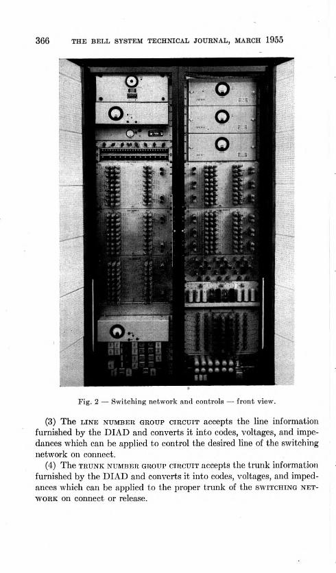
366 THE BELL SYSTEM TECHNICAL JOURNAL, MARCH 1955

I [ IliPfiiTO

n

O o

o

I

S- 'rcf?

Fig. 2 — Switching network and controls — front view.

(3) The line number group circuit accepts the line information furnished by the DIAD and converts it into codes, voltages, and impe- dances which can be applied to control the desired line of the switching network on connect.

(4) The trunk number group circuit accepts the trunk information furnished by the DIAD and converts it into codes, voltages, and imped- ances which can be applied to the proper trunk of the switching net- work on connect or release.

A TELEPHONE SWITCHING NETWORK AND ITS ELECTRONIC CONTROLS 3G7

H

Fig. 3 — Switching network and controls — rear view.

(5) The switching network passes on voltage marks from the marked line and trunk to trace idle paths on connect, provides a metallic talking path between line and trunk during the conversation, and re- leases the connection upon receipt of a release signal from the trunk number group.*

* It is interesting to note that after the connection is established, it is sufficient to furnish only trunk information to perform a release. This is true because the scries holding path from trunk to line constitutes a memory of what line and what crosspoints are associated with a particular trunk.

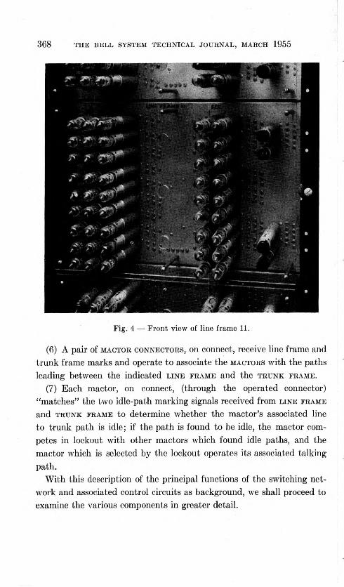
368 THE BELL SYSTEM TECHNICAL JOURNAL, MARCH 1955

m.

f< ? *****

- ^ *y

5 «

a ««■' _ ■

Fig. 4 — Front view of line frame 11.

(6) A pair of mactor connectors, on connect, receive line frame and trunk frame marks and operate to associate the mactors with the paths

leading between the indicated line frame and the trunk frame.

(7) Each mactor, on connect, (through the operated connector) "matches" the two idle-path marking signals received from line frame and trunk frame to determine whether the mactor's associated line

to trunk path is idle; if the path is found to be idle, the mactor com-

petes in lockout with other mactors which found idle paths, and the mactor which is selected by the lockout operates its associated talking

path. With this description of the principal functions of the switching net-

work and associated control circuits as background, we shall proceed to examine the various components in greater detail.

A TELEPHONE SWITCHING NETWORK AND ITS ELECTRONIC CONTROLS 369

Fig. 5 — Rear view of line frame 11.

THE SWITCHING NETWORK

The Switch Crosspoint

The basic building block of the switching network is the crosspoint. One crosspoint appears at each intersection of horizontal and vertical multiples. The packaging design of the crosspoint is such as to achieve maximum flexibility in the laboratory operation and testing of the net- work. The crosspoint has two parts, (1) a switch assembly using reed contacts, and (2) a small cold-cathode diode.

The crosspoint is shown on Fig. 7. It consists of four reed contacts or switches in an actuating coil with appropiatc mounting and connect- ing parts. Each reed contact consists of two 52 alloy* rods sealed in opposite ends of a piece of glass tubing containing helium gas. The contacting ends of the 52 alloy* rods are rhodium plated. The soft

* This is an iron-nickel alloy containing approximately 52 per cent nickel.

370 THE BELL SYSTEM TECHNICAL JOURNAL, MARCH 1955

steel cylinder housing the switch assembly (1) serves as a mechanical housing and a support for the plug and socket; (2) acts as a magnetic shield between adjacent crosspoints; and (3) acts as a partial return path for the magnetic circuit of the reed contacts. The plug on one end of the switch assembly serves to connect the crosspoint assembly to the external circuit, while the socket on the other end receives the cold-cathode diode. (Where the switch assembly is used as a simple relay, a short-circuiting plug replaces the cold-cathode diode.)

The operating margins of the switching network are to a large extent a function of the variation in diode breakdown and sustain voltages with

MACTOR LINE FRAME CONNECTORS TRUNK FRAME

LINE FRAME

13

1-27

IT 1-19

LINE FRAME

02

TRUNK FRAME

n

A I I u

TRUNK FRAME

2 L T\

L MACTOR 9 TO MACTOR CONNECTORS

I TO MACTOR

CONNECTORS _OCKOUT MACTORI

TRUNK FRAME INFORMATION

LINE FRAME NFORMATION

CONNECT OR

RELEASE LINE

NUMBER GROUP TRUNK

NUMBER GROUP

SWITCHING SEQUENCE CIRCUIT

LINE INFORMATION

TRUNK INFORMATION

TO DIAO THROUGH SWITCHING NUMBER GROUP CONNECTOR

Fig. 6 — Relation of switching circuits.

A TELEPHONE SWITCHING NETWORK AND ITS ELECTRONIC CONTROLS

QU IU< lUH CEZ

< 0 oQ J, O

Fig. 7 — Crosspoint assembly.

372 THE BELL SYSTEM TECHNICAL JOURNAL, MARCH 1955

age, temperature and also the variation from unit to unit. To assure satisfactory operation, electrical and life requirements were specified on the basis of the switching network needs and the A-167G diode was de- signed to meet these requirements. In designing the switching network, arrangements which would lead to overly severe requirements on the diode were avoided. The A-1676 diode is a simple, rugged structure which meets or exceeds the requirements in every regard.

Single Path Circuit

A single path through the switching network is shown on Fig. 8. In each of the four crosspoints, the general operation is the same. The cold- cathode diode in series with the coil in the control lead is used (1) to pass tracing voltages through idle paths while remaining an open circuit for busy paths and (2) to break up parasitic paths in parallel with operated crosspoints, and thus to avoid marginal release require- ments on the crosspoint relays. The reed contact in the sleeve lead, s, is used to establish a series path through the switching network for the purpose of holding the crosspoint relays of the selected path operated during the conversation. The reed contacts in the tip, t, and ring, r, paths are used to establish a series metallic path for signaling and talking between subscriber and trunk. Within the switching network the route of the tip and ring leads parallels that of the sleeve lead, and hence, tip and ring leads will not be shown or described in detail in the sections to follow. The fourth reed contact is used for display purposes only and has not been shown on Fig. 8.

In the following description of Fig. 8, a complete switching network is assumed, although for simplicity, branching paths have been indicated by "multiple whiskers". Starting from the idle condition, a path through the switching network is established as follows:

(1) Line frame and trunk frame identifying signals (marks of +130 v and -85 v, respectively) are applied to operate the proper connector relays to associate the mactors with the paths which go between the desired line frame and the desired trunk frame.

(2) A switch enabling mark (-85v) is applied to the idle A links lead- ing out of all line primary switches having the same switch number as the desired line.

(3) A vertical identifying mark (-i-isov) is applied to all lines having the same vertical number as the desired line.

(4) All diodes appearing between verticals marked in (3) and a links enabled in (2) break down and, in doing so, produce voltage shifts on the associated a links leading into the line secondary switches.

03

Ol m 2 - < LL q:_J UJ ^ >; Ztt ® i- < ^ u

—VW-i rvj - >

N i a. H < > (- = 2 9 5..- + SiO m Z 10

?<D P<

gR tu Z.-

2^ <Z = ■£ !?-iS N m < lu<2 Z2 y- a- z>o

V- 1/1 O (/I OUJ 1 tL D I± u J

—15< WV 5<5 - (M

; 2

iuJ t I. UJ , Z5C 3 < ^ u. u. — t-u- a

b£ 3 O

CO 5f E

ilH

373

374 THE BELL SYSTEM TECHNICAL JOURNAL, MARCH 1955

(5) The left contact on the line side mactor connector relay during step (1) has applied an enabling bias of - 155V to the control leads which lead out of the desired line frame to the mactors.

(6) The voltage shifts on the marked a links, in conjunction with the enabling biases of step (5), cause breakdown of idle line secondary diodes connecting between marked a links and the enabled b link control leads.

(7) Breakdown of the secondary diodes produces voltage shifts or marks which are fed on the control leads into the Li terminals of the mactors, each mark representing an idle path between the desired line and the mactor in question.

(8) On the trunk side, an enabling mark (+37v) is applied to all idle C links.

(9) A trunk mark (-I78v) is applied to the individual trunk to which connection is desired.

(10) As a result of (8) and (9), the trunk primary diodes representing connections between idle c links and the desired trunk are broken down, producing voltage shifts on these links.

(11) Each mactor, through an idle-test circuit, samples the voltage on its Ti lead, and, if this voltage indicates an idle b link, the mactor connects an enabling bias of +107V to its Ti and T2 leads.

(12) The voltage shifts on the marked c links, combined with the enabling biases applied by the mactors' idle-test circuits, cause break- down of all of the trunk secondary diodes representing idle paths usable for the trunk half of the desired connection.

(13) The breakdown of the trunk secondary diodes puts voltage shifts or marks on the Ti leads going to the mactors, each mark representing an idle path between the desired trunk and the mactor in question.

(14) Mactors which receive marks from both line and trunk sides in- dicate through a matching or coincidence circuit that their associated paths through the switching network between the desired line and the desired trunk are idle and available for use.

(15) The mactors which indicate a match energize their respective transistors, which compete in a common lockout circuit.

(16) The transistor which wins the lockout competition (i.e., achieves the fully conducting state) thereby selects the corresponding switching path for use.

(17) In response to the lockout operation, the selected mactor raises the current in both line and trunk halves of the selected path and operates the crosspoint relays associated with this path.

(18) During the conversation the selected path is held operated or "locked up" over the series sleeve lead path between ground on the line

A TELEPHONE SWITCHING NETWORK AND ITS ELECTRONIC CONTROLS 375

end of the connection and the -48v battery on the trunk end of the con- nection.

(19) The mactors are retired and the paths which were marked but not used are restored to normal by the removal of the line and trunk marks and the removal by the switching sequence circuit of various enabling voltages.

(20) At the completion of the conversation the connection is released by the temporary application of ground to the sleeve lead at the trunk, thereby bringing both ends of the holding circuit to the same potential and causing release of the crosspoint relays involved in the connection.

Regarding the holding circuit, it will be noticed that there is a 750-ohm resistor in series with the sleeve lead at the line end of the connection. This resistor simulates the winding of a cut-off relay. Hence, if a cut-off relay were required, it would be a simple matter to substitute the operate winding of a relay for the 750-ohm resistor.

A more detailed description of the control of the switching network is provided in Appendix I.

CHANNEL SELECTORS OR MACTORS

Functional Description of Mactors

As the description of the switching network has indicated, the mactors perform the functions of (1) matching of line and trunk idle-path trac- ing marks, and (2) selecting and connecting for use one of the idle paths revealed by the matching operation. To these general functions, in the present system, we have added the function of performing an idle-test on the b links of the switching network. The idle-test precedes the other portion of the mactor operation; hence, a mactor is enabled to continue its functions only if its associated b link is idle. Each mactor contains, as its principal elements, 4 cold-cathode gas tubes and a reed relay associ- ated with each, and a transistor. One gas tube and relay combination performs the idle-test; another combination receives the path tracing voltage from the line side of the switching network; the third such com- bination receives the path tracing voltage from the trunk side of the network; the transistor (in conjunction with those in other mactors) functions to select one of the idle paths for use, while locking out all others; and finally, the fourth gas tube and relay combination receives a triggering signal from the transistor and functions to establish a con- nection over the selected path. For a detailed description of how these functions arc performed, we refer the reader to Appendix II.

376 THE BELL SYSTEM TECHNICAL JOURNAL, MARCH 1955

Mactor Design Features

In general, the design of the mactor in the present system was based on maximizing the operating margins of switching network, rather than minimizing the amount of apparatus in the mactor. However, it should be noted that there are only as many mactors as there are alternate paths or channels in the switching network (3 in our scaled-down model, per- haps 10 in a full-sized office) and this means that the amount of apparatus in the mactors is a very small proportion of the total office equipment. The use of a separate idle-test, and the detection of line and trunk path tracing marks on different gas tubes lead to increased margins. The idle- test circuit used in the mactor is of particular interest because it uses a new grid-controlled cold-cathode tube, type M-1652. This tube, vi of Fig. 15, has control characteristics similar to those of a hot-cathode gas tube, while possessing all of the long life advantages of a cold-cathode tube in applications involving a low duty ratio. The main cathode, mc of vi also functions as a keep-alive anode, while kg is a keep-alive cath- ode. Discharge is initiated in this keep-alive gap by the application of —178 volts to terminal ce i a few milliseconds before the tube is required to respond to the control signal. At the same time the keep-alive gap is energized, the main anode, ma, is enabled by the application of +130 volts to terminal ae i. The tube is now ready to respond to a signal on its control grid. A negative potential of 20 volts or more on the control grid prevents transfer of discharge to the main gap while ground potential assures that transfer to the main gap will take place. In addition to the advantages of this tube from the standpoint of life, the fact that it will trigger on relatively small voltage shifts in high impedance circuits is utilized in the present circuit design.

The advantage from a margin standpoint of receiving line and trunk path-tracing marks on separate tubes may be understood if we consider what happens when these marks are received across the start gap of a single tube. It is evident in such a case that the variations of line and trunk path tracing marks must be summed in determining the least favorable circuit operating conditions. However, when the two marks are received on individual tubes, the marks are quantized before combin- ing or matching takes place, so that variations in the two marks are never added together.

Perhaps the most interesting design feature of the mactor is the nega- tive resistance lockout circuit using the switching transistor, type A-1608. In the usual operating routine, the lockout in this circuit is decided on a time basis; i.e., due to statistical time variations one transistor is operated and fully conducting before other transistors are energized. In the oc-

A TELEPHONE SWITCHING NETWORK AND ITS ELECTRONIC CONTROLS 377

casional "dead heat", a plurality of transistors can reach the high current condition together. In this case, it is significant to note that the transistor in each mactor has a high (29,800-ohm) base load resistance which gives it a negative emitter-to-ground impedance throughout the operating region. The emitter-to-ground impedances of the various mactors' transistors are connected in parallel, and this parallel combination is connected in series with a common lockout resistor (29,800-ohms). It can be shown that this circuit is unstable if more than one transistor is conducting in the operating region. Thus, even though two or more transistors should reach the operating region, one of them quickly as- sumes most of the circuit current and drives the other(s) into the quies- cent region of positive emitter-to-ground impedance and virtually zero emitter current. The maximum time required for one transistor to reach the high current state and drive the other(s) to the quiescent state is the "severance time". For the lockout circuit employed in the mactor, there is a severance time of approximately 0.5 microsecond. It is essential, of course, to avoid producing an output before the lockout has been re- solved. This requires that the circuit responding to the transistor have a minimum response time considerably exceeding the severance time. In the mactor circuit this is assured by the fact that the minimum triggering time of the cold-cathode tube, V3, is approximately ten microseconds. In addition, it will be noticed that there is a delay in response caused by feeding the transistor output, which occurs across the base load imped- ance, through an rc filter before placing it on the start cathode, sc, of vs. This rc filter was designed to have a delay great enough to take care, not only of the severance time, but also of possible temporary ambiguities caused by contact chatter in the L4 relays. These provisions result in a lockout circuit which is "a priori failure-proof".

FUNCTIONAL DESCRIPTION OF SWITCHING SEQUENCE CIRCUIT

The switching sequence circuit, see Fig. 16, is the common control circuit which functions whenever a connection through the switching network is established or released.

In the first case, when the switching sequence circuit receives an (es) establish signal from the switching information dispatcher, (1) it pre- pares the line number group circuit and trunk number group circuit to handle the coded signals on the line and trunk information leads (signals which correspond to the line and trunk to be connected together) (2) it applies operating voltage to the mactors, (3) it applies the connect trunk marking voltage to all the trunk frames of the switching network, and (4) it applies enabling bias to the c links of the switching network.

378 THE BELL SYSTEM TECHNICAL JOURNAL, MARCH 1955

After one of the idle paths between the line and trunk in question has been selected and the path established, the switching sequence circuit restores the number group circuits, mactors and mactor connectors to normal and removes the connect voltage mark and c link enabling bias from the switching network. The switching sequence circuit then trans- mits an ok signal to indicate to DIAD that the required connection has been made. Finally, the switching sequence circuit restores itself to normal.

In the second case, that in which the switching sequence circuit re- ceives a (ds) disconnect signal from the switching information dispatcher, the sequence circuit enables the trunk number group (to handle the sig- nals on the trunk information leads) and applies a release ground to the trunk number group elements. (As was noted earlier, a connection is released from the trunk side only of the switching network.) Sufficient time is allowed for the crosspoint relays in the path to release (about 10 milliseconds). Subsequently, the release ground is removed, and the trunk number group circuit is restored to normal. Finally, a pulse is sent out on the ok lead which signifies to DIAD that the path in question has been released and at the same time the switching sequence circuit restores itself to normal.

Connect and release cycles for the switching sequence circuit are de- scribed in detail in Appendix III.

SWITCHING NUMBER GROUP CIRCUIT

The switching number group circuit comprises the following parts: line vertical number group, line switch number group, trunk number group, and mactor connectors. All of these circuits have been skeletonized to conform with the skeletonized switching network. One of them, the line vertical number group, is shown in detail in Fig. 17, while other por- tions of the number group appear in block diagram.

The switching number group circuit performs two functions: (a) it decodes the signals on the line and trunk information leads from "2 out of 5" to "l out of 10" and (b) it provides the means for selecting and connecting to the proper points in the reed-diode switching network and for applying the several connect and release voltage marks. The number group circuits were designed on the basis that the signals on the line and trunk information leads are in the form of the equipment designa- tions of the line and trunk which are being served; that is, frame, switch and vertical. Each digit is indicated by the presence of +150V on two out of a group of five information leads, the other three leads being at +ioov.

A TELEPHONE SWITCHING NETWORK AND ITS ELECTRONIC CONTROLS 379

(In the quiescent state, all the information leads would be at +ioov, which means that no information is being supplied to the switching net- work.) The switching number group circuit is enabled and released by the switching sequence circuit. In setting up a connection, the switching sequence circuit applies +200V to the main anodes of the line number group digit tubes via the lng lead and +200y to the main anodes of the trunk number group digit tubes via the tng lead. On the release of a connection, only the trunk number group is enabled.

The decoding and selection operations of the number group circuit are described in Appendix IV.

COMPONENT AND CIRCUIT TESTS

Of the five types of cold-cathode gas tubes used in the design, three are essentially commercial products. These are the WE 376-B, the BTL A-1703, and the BTL A-1704. The latter two tubes are versions of the WE 425-A and WE 426-A without the plastic mounting flange and ex- ternal resistors.

The other two tubes types, the BTL A-1676 and the BTL M-1652 are not commercial products. The A-1676 diode which appears in each cross- point was tested as part of the tube design and development effort. Life tests on this gas diode gave a life expectancy of 3,000 active hours. Since the tube is used only momentarily each time a connection is established, this corresponds to an in-circuit life of 240,000 years. Such figures, of course, merely mean that a high degree of reliability may be expected in using this tube. The other non-commercial tube, the M-1652, is of in- terest because it is a grid-controlled cold-cathode tube which can be triggered reliably from low voltage, low power signals. The control char- acteristics of eleven of these tubes were measured in detail. Each tube was found to be suitable for use in the mactor circuit, where it is used as the idle-test tube. A typical control characteristic of one of these tubes is shown on Fig. 9.

Each reed-diode crosspoint was tested individually in four respects: (1) dc coil resistance, (2) insulation resistance, (3) operate and release current, and (4) operate and release time. The last two tests were made with positive and negative polarities of operate current and with con- tacts strapped in series and in parallel. The reversed polarity test estab- lished that any residual effect due to hysteresis in the magnetic material was very small. The operate and release tests with contacts in series and in parallel gave a measure of the total spread from the most sensitive contact to the least sensitive contact. Control limits were calculated for

I

380 THE BELL SYSTEM TECHNICAL JOURNAL, MARCH 1955

160

150

140 t/) O

130 UJ Q O 120 <

z <

no 5

100

90 -10 -9 -8 -7 -6 -5 -4 -3 -2 -1 0

CONTROL GRID IN VOLTS

Fig. 9 — Trigger characteristic of grid-controlled cold-cathode tube.

the data on dc resistance, operate and release currents, and operate and release times in order to reveal any crosspoints which were out of control in any of these parameters.

The switching number group, switching sequence circuit, mactors, line frames, and trunk frames were tested individually before being- interconnected. The tests consisted generally of making breadboard circuits which would apply the proper operating and information signals to the circuit under test. The test input information was then put through a variety of conditions calculated to exercise every element in the circuit.

Following the testing of individual circuits, they were assembled on the two switching bays, interconnected, and tests of the combined appa- ratus were made. Principally, these combined tests consisted of: (1) measurement of the timing of all of the important steps in establishing and releasing a connection, and (2) checking the satisfactory operation and release of paths involving all possible combinations of line, trunk, and interconnecting path.

Timing Measurements

The timing measurements were made by putting the switching net- work and control circuits through connect-release cycles repetitively at about 15 cycles per second, and observing operation on an oscilloscope. For the measurements which led to the sequence chart of the normal

\ \ \

\

\ ̂ '\ \

\ \ V O.X

s\

\ \ X '\ N

KEEP-ALIVE CURRENT IN MA

\ \ s \

A TELEPHONE SWITCHING NETWORK AND ITS ELECTRONIC CONTROLS 381

connect cycle, Fig. 10, the sweep of the oscilloscope was triggered from the es pulse which starts the connect cycle.

Taking the start of the connect cycle as zero on the time scale, and the times in milliseconds, the following relations are apparent: (1) at t = 4, the major control circuits; (line number group, trunk number group, and mactors) receive their enabling voltage from the switching sequence circuit; (2) at i = 6, the line and trunk number groups operate; (3) at t = 8, the mactor connector relays operate; (4) at t = 10, the mactors complete their idle-tests, receive voltage marks from line and trunk sides of the path, and one or more of them returns to the switch- ing sequence circuit a "match" signal (ms); (5) at t = 12, the mactor lockout circuit operates to perform the path selection, and the current is increased in the selected path; (6) at t = 13, the crosspoints in the selected path operate; (7) at t = 15, the main anode voltage is removed from vi of the switching sequence circuit; (8) at t = 19, the enabling voltages are removed from the number groups and mactors; (9) at t = 23, the main anode voltage is re-applied to vi of the switching sequence circuit; (10) at t = 23, the switching sequence circuit sends an ok signal

CONNECT PULSE (ES)

SWITCHING SEQUENCE <

CIRCUIT

NUMBER . GROUPS'

ENABLE VOLTAGES (TC, TSE. LNG, AE 1,.A E 2)

SWITCHING NETWORK•

PATH

MAIN ANODE VOLTAGE ON VI

OK SIGNAL

NUMBER GROUPS' OPERATION

MACTOR CONNECTORS I r

MACTOR OPERATION

t- MATCH SIGNAL (MS)

LOCKOUT PATH SELECTION

SELECTED PATH OPERATION

0 2 4 6 10 12 14 16 18 20 22 24 26 28 30 32 34 36 38 TIME IN MILLISECONDS

Fig. 10 — Connect cycle when call is completed.

382 THE BELL SYSTEM TECHNICAL JOURNAL, MARCH 1955

SWITCHING SEQUENCE

CIRCUIT

NUMBER GROUPS

MACTORS

0 2 4 6 8 10 12 14 16 18 20 22 24 26 28 30 32 34 36 38 TIME IN MILLESECONDS

Fig. 11 — Connect cycle when call is blocked..

through the switching number group connector to the switching infor- mation dispatcher, indicating that the switching network and controls are ready for a new connect or disconnect operation. The above cycle description assumed that an idle path was found.

The time relations which were measured with all usable channels busy are shown on Fig. 11. In this case, no idle path is found and the cycle differs from the above beyond (3), as follows; (4) at t = 10, the mactors complete their operation without finding an idle path, and therefore without sending a match signal to Switching Sequence Circuit; (5) at t = 28, the time-out circuit removes main anode voltage from vi of the switching sequence circuit; (7) at t = 34, number groups, mactors, and mactor connectors release; (8) at t = 36.5, main anode voltage is re- applied to vi and the switching sequence circuit sends a block signal through the switching number group connector to the switching infor- mation dispatcher, indicating that the desired connection could not be obtained, but that the switching network and controls are ready for the next operation.

The disconnect cycle has only one possible sequence, since there is no question of blocking forcing the system into an alternate cycle. The dis- connect cycle is simpler, too, since the connection is released from the trunk end alone. Thus, the line number group and mactors are not re- quired to function on a release operation. Time readings on the release cycle, which are displayed in the form of a sequence chart on Fig. 12,

CONNECT PULSE (ES

VO LTAC ,ES rc.i SE LNG TN 3, A Elr \E2

SIC .NAl 1—

ENABLE

MAIN ANODE OF V

BL .OCE

NUN /BE GP OUF S' 0 ̂ ER/ \TIO N

MACTOR CONNECTORS

MA O t- o ^S IDLE TE ST

1 1 COMPLETED 1 1

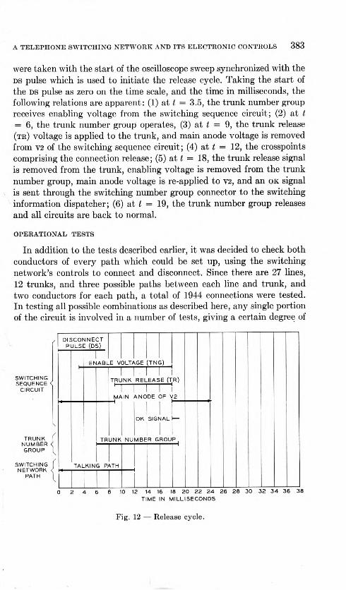
A TELEPHONE SWITCHING NETWORK AND ITS ELECTRONIC CONTROLS 383

were taken with the start of the oscilloscope sweep synchronized with the ds pulse which is used to initiate the release cycle. Taking the start of the ds pulse as zero on the time scale, and the time in milliseconds, the following relations are apparent: (1) at t = 3.5, the trunk number group receives enabling voltage from the switching sequence circuit; (2) at I = 6, the trunk number group operates, (3) at t = 9, the trunk release (tr) voltage is applied to the trunk, and main anode voltage is removed from V2 of the switching sequence circuit; (4) at t = 12, the crosspoints comprising the connection release; (5) at ^ = 18, the trunk release signal is removed from the trunk, enabling voltage is removed from the trunk number group, main anode voltage is re-applied to V2, and an ok signal is sent through the switching number group connector to the switching information dispatcher; (6) at t = 19, the trunk number group releases and all circuits are back to normal.

OPERATIONAL TESTS

In addition to the tests described earlier, it was decided to check both conductors of every path which could be set up, using the switching network's controls to connect and disconnect. Since there are 27 lines, 12 trunks, and three possible paths between each line and trunk, and two conductors for each path, a total of 1944 connections were tested. In testing all possible combinations as described here, any single portion of the circuit is involved in a number of tests, giving a certain degree of

SWITCHING SEQUENCE <

CIRCUIT

I

TRUNK f NUMBER < GROUP |

SWITCHING | NETWORK <;

PATH 1

0 2 4 6 8 10 12 14 16 18 20 22 24 26 28 30 32 34 36 38 TIME IN MILLISECONDS

DISCONNECT PULSE (DS)

ENABLE VOLTAGE (TNG)

TRUNK RELEASE (TR)

MAIN ANODE OF V2

OK SIGNAL I

TRUNK NUMBER GROUP

TALKING PATH

Fig. 12 — Release cycle.

384 THE BELL SYSTEM TECHNICAL JOURNAL, MARCH 1955

redundancy. Nevertheless, a full testing schedule was considered desir- able in the present instance for two reasons: (1) the operate and hold characteristics of crosspoints in a marginal case can be a function of how they are combined (i.e., crosspoints x and ij could operate satisfactorily in different paths, but fail to operate in a path which involved both of them); and (2) a full test increased the likelihood of discovering any incipient troubles. In testing a larger switching system by this method, the total number of operations required and the degree of redundancy associated with a full test would be excessive. In such a case the ideal test would operate on a fully automatic basis and would follow an abbreviated schedule which would test each element of the switching system the desired number of operations only.

PERFORMANCE OF NETWORK AND CONTROLS

For forty-two months the switching network and controls were oper- ated to gain information on reliability. The results of this operation are summarized briefly on Fig. 13. The left column lists the major circuits which required adjustment or replacement of elements. The second and third columns, give, respectively, element replacements made as a result of preventive maintenance and those made as a result of equip- ment failures. Most of the germanium diodes which were replaced were used as relay contact protection. Diodes used as logical combining ele- ments have functioned reliably with no failures. Three means of im- proving the situation regarding diodes used as contact protection are: (1) install all diodes on plug-in mounts so preventive maintenance can catch incipient troubles, (2) use a diode with a higher inverse voltage rating, or (3) use resistance-capacitance contact protection. The ger- manium diode failure rate diminished with time, indicating that we were weeding out the weaker diodes. Early in the tests the diodes were trans- ferred to plug-in mounts; therefore, most later diode replacements were made as a result of routine maintenance tests without incurring circuit failures.

Twenty-eight vacuum tubes were replaced during the tests. Ten were replaced as a result of circuit failure while eighteen were replaced as a result of routine tests. All of these vacuum tubes were used in the regu- lated power supplies. To catch weak tubes before they produced failures, the following monthly power supply regulation check was applied. With 80 per cent of the maximum rated load applied, the power supply out- put voltage should not sag more than 3 per cent. If a power supply passed this test, no further check was made. If it failed, tubes were

A TELEPHONE SWITCHING NETWORK AND ITS ELECTRONIC CONTROLS 385

CIRCUIT SERVICED

ELEMENTS REPLACED

ON ROUTINE BASIS

ELEMENTS REPLACED BECAUSE OF CIRCUIT

FAILURE

TYPE OF ELEMENTS RESPONSIBLE FOR SERVICING

REMARKS

POWER SUPPLIES 18 10 VACUUM TUBES

TYPE REQUIRING MOST REPLACEMENTS". SERIES REGULATOR TUBES,6Y6

NUMBER GROUPS 9 24 POINT CONTACT

GERMANIUM DIODES 18 DIODES FAILED SIMULTANEOUSLY DUE TO ABNORMAL POWER VOLTAGE. DIODES TYPE 400E

SWITCHING SEQUENCE

CIRCUIT - 2 POINT CONTACT GERMANIUM DIODES

2 DIODES TYPE 400E HAD LOW BACK RESISTANCE; REPLACED WITH GERMANIUM AREA JUNCTION DIODES

TRUNK FRAMES - 5 POINT CONTACT

GERMANIUM DIODES DIODES IN TRUNK HOLDING CIRCUIT (TYPE 400E) OPEN CIRCUITED

GENERAL - - COLD CATHODE GAS TUBES

BREAKDOWN TIMES ERRATIC; LIGHTS INSTALLED TO PROVIDE INITIAL PHOTO-IONIZATION

Fig. 13 — Maintenance summary.

checked individually and replacements made as needed. Vacuum tube failures were the chief source of trouble requiring further design effort. The higher degree of power reliability which would he necessary in a commercial system could be achieved by (1) duplicate power supplies with automatic switching to the spares, and (2) by designing individual supplies to a higher order of reliability.

Early in the tests, we discovered that gas tube breakdown times were longer and more erratic than desired. We know that all cold-cathode tubes for their operation depend on a small residual ionization. In the tubes we used, this ionization was provided by a small smear of radium bromide in each tube. The ionization from this source alone proved in- sufficient to assure stable sensitivities and breakdown times. Therefore, we installed three line-type incandescent light sources of GO watts each behind the dividing strips of the bays. The resulting photo-ionization produced very consistent tube performance.

Despite the troubles mentioned above, the overall reliability of the switching network and controls has been very satisfactory. Examination of our maintenance log reveals only 23 circuit failures in 42 months, most of the failures occurring early in the test. In particular, the re- liability of the cold cathode gas tubes, mercury relays and reed relays has been outstanding. Where germanium diodes function in logic circuits,

386 THE BELL SYSTEM TECHNICAL JOURNAL, MARCH 1955

we have encountered no failures. The transistor lockout circuit which performs the channel selection has operated throughout the period of test without any transistor replacements.

CONCLUSION

The construction and testing of a 27-line, 12-trunk model of a telephone switching network and its associated electronic control circuits and their operation in the laboratory for over three years have demonstrated the technical feasibility and the reliability of the basic design. On the basis of 50,000 calls per busy hour and 57 per cent active time of the control circuits, this network and its controls are fast enough to permit one-at-a- time operation in a busy 10,000 line telephone exchange. In the design of this skeletonized model, one of the objectives achieved was the use of relatively simple components having practical tolerances. Although the network and its controls were designed specifically for the DIAD telephone system, these circuits are sufficiently flexible that they could be adapted to other information handling systems such as digital com- puters.

ACKNOWLEDGEMENTS

A number of people have helped to make this high-speed network and its controls a success. We wish specifically to acknowledge the contribu- tions of E. Bruce to the basic reed-diode network and to the series- marking method of control. B. G. Bjornson designed the transistor lockout circuit used in the mactor. D. S. Peck and W. G. Stieritz de- signed and tested the A-1676 gas diode. The mechanical design of the crosspoint element and other parts is the work of J. F. Midler. L. Maggi and L. J. Robinson assembled and wired the equipment and assisted in the testing.

Appendix I

THE SWITCHING NETWORK AND ITS CONTROL

The switching network and mactors are shown on Fig. 14. The net- work is laid out in standard 4-stage fashion except that the entire circuit is skeletonized. Thus, a network which might contain 10,000 lines and 2,000 trunks in a large office is scaled down to contain 27 lines and 12 trunks. In Fig. 14 only one line frame and one trunk frame have been shown. The other line frames and trunk frames would be similar to those shown. The numbering of lines, switches and frames is such as to

o

M-

I

P P ci- 3 p

g° i n ^

t/z

m

(D -I

rn...

!u -H W

11

r

zo PS

It, M I

i:::. i I I

la M I

m.

rU

// // / z / ?? c« s iff

T

iKyv /" -

\0ri

S0t- N-—-X C±D |g^-z T

C T 0- SN^ NN-

-A/W— I D H

m:

-AAA— o O 3

S? 'J'

—WV— ■ a H

;tJ]:

CO

n rr m H < ni O'

la In I

[itr

£|» WV*-VvV - VWr^WV 131 IH I

nil ih

n " mC ££ m® Z0

J CO n? nx

A TELEPHONE SWITCHING NETWORK AND ITS ELECTRONIC CONTROLS 387

indicate the full-sized office on which the skeletonized model is based. In the body of this article we described the operation in terms of a single path through the switching network. Now we will see how this descrip- tion applies when we consider the complete switching network.

As a specific example, let us assume a connection is desired between the line appearing at vertical 50 on switch no. 8 of line frame 13 and the trunk appearing at vertical 4 on switch is of trunk frame 7. This line and trunk appear near the top of Fig. 14. Leads involved in estab- lishing and releasing a connection between this line and trunk have been shown by heavy lines on Fig. 14.

At the bottom center of Fig. 14 there are leads which carry line frame and trunk frame information on the basis of which the proper mactor connector relays may be operated. In the example we are con- sidering, the lfi3 and tf? leads would be energized, thus operating the two mactor connector relays which are shown on Fig. 14. Their operation associates the mactors with the b links extending between line frame 13 and trunk frame 7. Now let us examine the line frames and see how the proper line terminal is marked. This is done by first applying en- abling voltage to the idle a links of the desired switch and all other switches having the same switch number, and then applying marking voltage to the proper vertical number on all line primary switches. Since both of these voltages are required to produce breakdown in the line primary diodes, only diodes associated with the desired line or with similar numbered lines on other line frames are broken down. Referring again to Fig. 14, at the bottom center of the line frame are line switch leads designated ls n, ls 5, ls 8. In this case, the ls 8 lead is energized, resulting in the application of an enabling bias to the idle a links leading out of line primary switches numbered 8 on all line frames. At the bottom left of Fig. 14 are terminals designated lv sc, lv 09, and lv oo. In our present example, lv 56 has a marking voltage which is applied to vertical 56 on every line primary switch. However, since only the line switches numbered 8 have enabling marks on their links, the vertical mark is effective in breaking down only the crosspoint diodes associated with vertical 56 on line primary switches 8 of each line frame. At this point, it should be noted that if any of the a links had been busy, the voltage on the links would be determined primarily by the holding circuit of the busy path (which has a low impedance) rather than the link enabling voltage, which passes through a 100K link resistor. This link voltage for busy paths is arranged to act as a bias which prevents the breakdown of primary diodes. This same method of marking links busy applies to the c links.

388 THE BELL SYSTEM TECHNICAL JOURNAL, MARCH 1955

wv

11

"7

WV m ii 3^

AAA—VVv—

wH

vaH D O u) U {/) O lii

7

\ HH

uj

—n—o—VvV

~^-o-V\A-

O Q- zn > T

T1 IM P -z __ >•- (0 3 O UJ * *

WV u <

WV

A TELEPHONE SWITCHING NETWORK AND ITS ELECTRONIC CONTROLS 389

The foregoing paragraphs have described the process of marking the idle line links. In the ensuing description, let us assume that all of these links were found idle, and therefore were marked. The marks or voltage shifts are passed on to the appropriate inlets of the various line secondary switches of the line frames, here represented by ls i, ls 4, and ls 9 on LINE FRAME 13.

It will be noted that the line side relay of the mactor connector pair, when it operated, applied an enabling mark of -issv to the control leads of the b links leading out of line frame 13 toward trunk lead 7. Inter-frame links which go to other trunk frames or which come from other line frames receive no enabling marks and hence cannot be marked in the next step of the path tracing operation.

As a result of the marks appearing at the inlets of the line secondary switches, plus the enabling marks applied by th^ mactor connector relay, the secondary diodes which could be used in establishing the desired line-to-trunk path are broken down. (Note that secondary diodes on frames other than line frame 13 are not broken down because of the absence of the -issv b link enabling signal.) The breakdown of second- ary diodes on line frame 13 places path tracing marks on the corre- sponding control leads which pass through the contacts of the left mactor connector relay. These marks then proceed to the Li terminals of the various mactors. In this case, the marks from ls 1, ls 4 and ls 9 go, respectively, to mactors 1, 4 and 9. This completes the path tracing and marking operation for the line half of the connection.

The marking of the trunk half of the connection (again see Fig. 14) is similar to the marking of the line half of the connection in general principle but varies somewhat as to specific detail. First, all of the idle c links are enabled by the application of +37V to the terminals marked tse on the trunk frames. (Those c links which arc busy remain at a voltage which is determined by the division of the -48V holding battery in the busy paths.) Then a -85V trunk frame and vertical identifying signal is applied to the terminal tfv 74 while a trunk switch identifying signal of +130V is applied to terminal ts 15. As a result of these two sig- nals, a trunk number group element shown at the top right of Fig. 14 is selected and operated. The other elements have either no signals applied, or a signal on one side only, and hence do not operate. The switching sequence circuit then applies a "trunk connect" voltage of -178V to terminal tc. This voltage is passed up the number group multiple, through the connect contact of the operated number group relay, and placed on the control lead of vertical 4 of trunk primary switch 15 on trunk frame 7. The trunk connect voltage, in connection with the

390 THE BELL SYSTEM TECHNICAL JOURNAL, MARCH 1955

enabling voltage on idle c links, results in the breakdown of all primary switch diodes connecting between the marked trunk and the enabled links. The breakdown of these diodes places a voltage shift, or mark, on the idle links connecting trunk primary switch is to the various trunk secondary switches of trunk frame 7. For purposes of further descrip- tion, we will assume that all of the c links extending from trunk primary switch 15 to trunk secondary switches of trunk frame 7 were idle and hence received path tracing marks.

We will leave the path tracing marks for the time being and consider what is happening on the trunk side of the mactors and mactor con- nectors. It will be recalled that a pair of mactor connector relays has operated. The contacts on the trunk side mactor connector relay extend control leads from the trunk secondary switches of trunk frame 7 to the mactors. The control leads which are thus extended are those asso- ciated with the b links going from trunk frame 7 to line frame 13, the frames on which the desired trunk and line appear. The control leads are carried to the Ti and T2 terminals of the various mactors. In this par- ticular case, the control leads from trunk secondary switches 1, 4 and 9 are associated with mactors 1, 4 and 9 respectively. By means of an idle-test circuit which is a part of each mactor, the mactors examine the voltages on their Ti terminals. Voltages of approximately —24 volts at these points represent busy b links and prevent the idle-test circuits from functioning, while ground voltages represent idle paths and trigger the idle-test circuits. Assuming that each of the b links under test was found to be idle, each mactor idle-test circuit applies an enabling mark of -(-i07v to its Ti and T2 terminals. These enabling marks travel back over the mactor connector multiple and through the contacts on the mactor connector relay to reach the control terminals of the appropriate links leading from trunk secondary switches 1, 4 and 9. These en- abling marks, in connection with the path tracing marks which earlier were placed on the c links, cause breakdown of the trunk secondary diodes of the crosspoints which receive both of these signals. The break- down of these trunk secondary diodes extends the idle-path tracing marks to the Ti terminals of the mactors. In the case we are considering, the marks from ts 1, ts 4, and ts 9 are received on the Ti terminals of mactors 1, 4 and 9, respectively.

The mactors at this point have idle-path tracing marks on their Li terminals and also on their Ti terminals. Each mactor performs a match of these two marking voltages and thereby indicates the idle or busy status of the corresponding path between the desired line and trunk. Assuming that the match indicates the path to be idle, each mactor

A TELEPHONE SWITCHING NETWORK AND ITS ELECTRONIC CONTROLS 391

energizes its portion of the common transistor lockout circuit. The lockout circuit is designed so that only one transistor can remain in the conducting state. In this case, we will assume that it is the transistor in mactor 9 which conducts and selects the path, and that mactors 4 and i are locked out. mactor 9 then shorts out resistance in series with its Li and Ti terminals, thereby operating the 4 reed-diode crosspoints in its associated line to trunk path. The operated path is the one running across the top of Fig. 14 whose central link extends between line sec- ondary switch 9 and trunk secondary switch 9. The operation of the various crosspoint relays comprising this path establishes a metallic holding path between ground on the line end of the connection and -48v on the trunk end of the connection. The various enabling and marking voltages which were applied to the switching network by the switching sequence and number group circuits are now removed. Removal of these voltages causes the various gas tubes shown on Fig. 14 to de-ionize and restore to normal, while the newly operated path remains locked up to the -48v battery.

When it is desired to release the connection after the conversation is completed, the trunk number group is operated. Referring to Fig. 14, the trunk to be released is selected by the application of -ssv to terminal tfv 74 and +130V to terminal ts is. These two voltages operate a trunk number group element shown at the top right of Fig. 14. Then the switching sequence circuit grounds the tr lead and this ground is passed up the number group multiple, through a contact on the operated number group element, and onto the sleeve lead of the trunk. Ground appearing on the sleeve lead reduces the holding voltage to zero, and the crosspoint relays comprising the path release, freeing the crosspoints and links involved for subsequent use. Ground is now removed from the tr terminal, and the -ssv and +130V signals are removed from terminals tfv 74 and ts is, respectively. The previously operated trunk number group element releases, and at this point the entire switching network and controls are back in the original state.

Appendix 11

Mactor Operating Cycle

The mactor operating cycle may be followed by referring to Fig. 15. The sequence is as follows:

(1) Anode and cathode enabling voltages of +130V, ground, and -178V are applied by the switching sequence circuit to terminals ae i, ae 2, and ce i, respectively.

392 THE BELL SYSTEM TECHNICAL JOURNAL, MARCH 1955

(2) Through the operation of the appropriate mactor connector the Li terminal, and the Ti and T2 terminals are associated with control leads from the line frame and trunk frame, respectively, of one of the b links which could be used for the desired connection.

(3) If a particular b link is busy, a potential of about -24v appears on Ti, and hence on the control grid (cg) of vi, preventing transfer of the discharge to the main cathode-anode gap (mc-ma) ; however, assum- ing the b link to be idle, ground potential appears on cg via Ti. causing the transfer of discharge in vi to the mc-ma gap and causing the operation of relay li.

(4) Operation of relay li applies +107V to terminals Ti and Ta to enable the control leads associated with the trunk side of the b link and also extends the connection from terminal Li down to the start anode, sa, of V2.

(5) Assuming the line half of the path through the switching network to be idle, a path tracing mark of 0 volts (nominal) appears at the normally negative start anode, sa, of V2, initiating a discharge from this electrode to the mam cathode, mc.

(6) Discharge in V2 shifts to the main gap (mc-ma), thus operating relay L2.

(7) Operation of relay L2 applies -3GV to the main cathode of V4 and also extends the control terminal, Ti, to the start cathode, sc, of v4.

(8) Assuming the trunk half of the path through the switching net- work to be idle, a path tracing mark of -48V (nominal) appears at terminal, Ti, whence it is connected to the start cathode, sc, of V4.

(9) The appearance of -48v on the start cathode, sc, in conjunction with the +130V on the start anode, sa, causes the start gap of V4 to break down.

(10) With the start gap broken down, the discharge in V4 transfers to the main cathodc-to-anode gap (mc-ma), operating relay L4,

(11) Operation of relay L4 sends the switching sequence circuit a "match" signal of +107V via the terminal labeled MS, to indicate that the mactor has found its complete line-to-trunk path idle; operation of L4 also places the mactor's transistor in lockout competition with those in other Mactors by energizing the collector of the transistor with -G7V.

(12) Assuming that this transistor wins the lockout competition, it will go to the high current condition, and, in doing so, will produce in the common lockout resistor a voltage drop which will prevent transis- tors in other mactors from reaching the high current condition.

(13) The high current condition produces a negative voltage at the base, b, of the transistor, which negative voltage is passed to the start cathode, sc, of vs, initiating discharge in its start gap (sc-sa).

A TELEPHONE SW ITCHING NETWORK AND ITS ELECTRONIC CONTROLS 393

(14) Discharge in vs transfers to the main gap (mc-ma), operating relay L3.

(15) Operation of L3 increases the current and causes the crosspoint relays to operate in the line and trunk halves of the selected path through the switching network.

(Ifi) Previously applied enabling voltages appearing at terminals ae i, ae 2, and ce i are removed from the mactor by the switching sequence circuit, interrupting discharges in tubes vi, V2, and V3 and re- leasing relays li, L2 and L3.

(17) Release of L2 interrupts discharge in V4 by removing voltage from its main cathode, mc, while simultaneously causing relay L4 to release.

(18) During the release of the various relays, the ne-2 cold-cathode diodes absorb some of the inductively stored energy, thus limiting the magnitude of voltage transients.

(19) After a deionization time of a few milliseconds, the entire mactor is again in its normal state and ready to function on a new call.

(20) Because the connection which was just established remains held up over the sleeve lead's series metallic path, it requires no further servicing from the mactor.

Appendix III

DETAILED DESCRIPTION OF SWITCHING SEQUENCE CIRCUIT

Conned Cycle

Refer to Fig. 16, which shows the switching sequence circuit. On "connect" the voltage on the es lead rises abruptly from approxi- mately +ioov to +150v. This causes the control anode of tube vi to rise momentarily from ground to +50V. Thereupon, vi fires, conduction trans- fers to its main gap, and the two mercury contact relays Li and L2 operate. However, before li and L2 operate, the switching number group con- nector operates and applies the appropriate signals to the information leads of the number group. The operation of li: (a) enables all the trunk primary switches by applying +37V to the idle c links over the tse lead, and (b) enables the line and trunk number group decoding tubes of the switching number group circuit by applying +200V to their main anodes over the lng and tng leads. Relay L2 applies -i78v, +130V and ground to the mactors, +130V to the time-out tube (vs) and -i-isov to the match tube (v4) and -i7sv connect mark (tc) to the trunk frames.

If there is at least one idle path available, the mactor or mactors so indicate by applying +107V to the ms lead of the switching sequence circuit. This voltage fires the match tube, V4, which operates relay L4.

TSE \ TO TRUNK FRAMES

LNGs TO SWITCHING

TNG ( NUMBER GROUP

TR TO TRUNK TC ( FRAMES

TO MACTORS

TO block) switchinc ^ NUMBER

GROUP CONNECTOI

R 3 2000 Wv

10 K 0,1 MF

RI I00K

+ 37 V +200 V

C; L2 Trn

-46V > -176 V AE2 At 1

Z 2 2400

2 2

R4 '0^

R 9 MS I TO rMACTORS - C2 0.25 MF

cr 'J 560

L5 V5 RI3

OOK -48 V

2 > o ■p CC <. RI4

L4 -esv +150 v V 7 R20 R2I I—vw

2400 2400 +200V -48V RI5 ids; t- < O

S ? S <. C4 DS V2 18K 0.1 MF

1 RI9 I00K <\i > o (\j . en rr < r)

+200V -46V -46V

l

■n

vio .)

R23<- ISK.-'

+ 200V

| 1 I 1 -asv +i5ov

>R25 >560

TO 0K \ SWITCHINI

' ■ / NUMBER ) GROUP

CONNECTO

R24 > 18 K *GE NE-2

-esv +i50v

Fig. 16 — Switching sequence circuit. 394

A TELEPHONE SWITCHING NETWORK AHD ITS ELECTRONIC CONTROLS 395

When relay ja operates, it removes the +200V from the main anode of vi and at the same time starts the charging of condenser cg through resistance ris. Tube vi stops conducting and relays li and L2 release. In releasing, these relays remove the +37V and -178V connect marks from the trunk frames, remove +200V from the switching number group circuit, remove -178V, ground and +130V from the mactors and remove +130V from tubes vs and V4. During the approximately 7 milliseconds required to operate relay L4 and release relays li and L2, the crosspoint relays of the talking path are being operated.

After the switching number group and mactors are disabled and all the "connect" voltages are removed from the switching network, the connection is held up between -48v and ground via the sleeve lead. After relay L2 releases, relay L4 releases, thereby restoring +200V to the main anode of vi. At the same time condenser ce, which had become charged between +150V and -85v (to a total emf of 235 volts), is dis- charged through gas diode V7. This discharge current develops a negative voltage pulse across resistance Ri7 about 60 volts in peak amplitude and approximately 0.3 millisecond in duration. Thus, the voltage on the ok lead drops momentarily from +150V to +90V, and this voltage shift is transmitted via the switching number group connector to the DIAD circuits, indicating that the connection called for has been made and that the switching sequence circuit is back to normal and ready to handle another connect or release.

It is recognized that the match (ms) signal does not furnish a positive check that the path has been closed through from line to trunk. How- ever, since this can be verified later as a part of supervision, it was felt the extra time and increased circuit complexity required to make a positive determination that tip and ring are connected through the switching network was not justified.

In connection with the circuit for generating the match signal, it should be noted that one of the purposes of resistance rig is to prevent tube V7 from firing when the contacts of mercury relay L4 are "bunched" on operate. (The voltage, being divided between resistances ris and rig, is not high enough across rig to break down V7, which has a nominal breakdown of isov.) Also, rig completes the discharge of cg after its potential has dropped below the sustain voltage of V7.

If no complete idle path is available between the line and trunk in question, none of the mactors will be fully operated; that is, none of the L4 relays in the mactors will be operated. Thus, no match signal will be sent out by the mactors and condenser C2 in the switching sequence circuit will continue to charge toward +13OV through the series-parallel

396 THE BELL SYSTEM TECHNICAL JOURNAL, MARCH 1955

combination of R5, rg, Z2, and za until the potential across C2 reaches the breakdown voltage of the control gap of vs. This occurs about 25 milli- seconds after the appearance of the es signal. V3 fires, conducts in its main gap and relay L5 operates to perform in the same way as did relay L4 to restore the number group circuit, mactors, and switching network to normal and release relays li and L2. Relay ls also initiates the charg- ing of condenser C3 through resistance rs. Relay L2 in releasing removes voltage from V3, allowing it to de-ionize and relay L5 to release. When L5 releases, condenser cs discharges through gas diode V5 and a 60v (nega- tive) pulse similar to the ok signal appears on the block lead to indicate that the connection called for was not made. At the same time, voltage is restored to the main anode of tube vi and the switching sequence circuit is thus ready to accept another connect or release signal. While relay L5 is releasing, condenser C2 is discharged through resistance R4 and the series-parallel combination of rs, rg, Z2 and zs.

When the es signal is removed, that is, the voltage on the es lead drops abruptly from +150V to +ioov, condenser ci is discharged rapidly due to the low forward conducting resistance of the germanium varistor zi in parallel with resistance ri.

The two small gas diodes vs and vo which are connected in series across relays li and L2 have a nominal breakdown of oov and are em- ployed to limit the inductive voltage developed by the windings of these relays on release, without substantially increasing the relay operate or release time.

Release Cycle

The indication that a connection through the switching network is to be released is an abrupt rise in voltage on the ds lead from its normal potential of +ioov to +I50V. This abrupt rise fires gas tube V2 which operates relay L3. Relay ls (a) applies +200V to the trunk number group and (b) operates relay lg. Before the contacts of relay lg close, however, the trunk number group functions and the number group element cor- responding to the trunk in question is operated. Then relay lg applies re- lease ground (via a contact on the trunk number group element) to the trunk sleeve terminal. This reduces the holding voltage on the control path of the connection through the switching network to zero, causing the crosspoint relays to release.

The operation of relay lg also starts the charging of condenser C5 through resistance R23, and interrupts operating current to tube V2 and relay L3. When L3 releases it de-energizes lg and removes a connection of +200V from the trunk number group. (However, the trunk number

A TELEPHONE SWITCHING NETWORK AND ITS ELECTRONIC CONTROLS 397

group is still receiving +200V through lg.) Relay lg in releasing: (a) re- moves release ground from the trunk control terminal, (b) removes -(-200V from the trunk number group, (c) restores main anode voltage to tube V2 (which meanwhile has become de-ionized) and (d) allows con- denser C5 to discharge through gas diode vg and produce a gov negative pulse on the ok lead in the same way that the "connect" ok pulse is generated. About a millisecond following the ok pulse, the trunk number group releases. However, the switching sequence circuit is ready to handle another connect or release just as soon as the ok pulse appears, since the trunk number group is restored to normal before any of the relays li, L2 or L3 could be re-operated on a subsequent es or ds signal.

The sequence of operation in applying and removing the release ground is designed so that the relatively heavy release current (100 ma) is established and interrupted with mercury contacts instead of reed contacts of the trunk number group element. The release ground is held on the trunk for sufficient time to insure the release of the switching path crosspoint relays.

As in the case of a connect, no positive check of the release of the path is made and for much the same reasons.

The gas diode vio (nominal breakdown gov) limits the inductive voltage surge from the winding of relay lg without substantially in- creasing either its operate or release lime.

Appendix IV

DETAILED DESCRIPTION OF SWITCHING NUMBER GROUP CIRCUIT

Decoding

The decoding is accomplished by means of varistor-resistor networks and sensitive cold-cathode gas triodes. For an example, let us look at the Fig. 17, where the line vertical units digit of our skeletonized version is represented by the LV2, lv4 and lv? leads (5 would be required for a full digit lvo, lvi, LV2, LV4, and lv?). Let us assume that the LV2 and LV4 leads are at -hgov, while the LV7 lead is at +ioov. Furthermore, let us note the following circuit conditions: (a) the backward resistance of the varistors zs, Z4, etc. is greater than 100,000 ohms, (b) the forward resist- ance of the varistors is less than 1,000 ohms, (c) the resistance of the resistors R3, R4, etc., is 0.5 megohm ± 5 per cent, (d) the breakdown voltage of the control gap of the gas triodes lvg, lvg, and lvo varies from 62 to 89 volts, (e) the impedance of each source supplying voltage to the

398 THE BELL SYSTEM TECHNICAL JOURNAL, MARCH 1955

information leads is approximately 5,000 ohms, and (f) the bias voltage on the gas triodes is +50V ± 3 per cent. Under the foregoing conditions, the control anode of tube lvb will rise to a potential sufficient to fire the control gap of lvg, while the control anodes of lvo and lv9 will remain below the potential required to fire their control gaps. While we have supplied only three input leads and three output digits in our skeletonized number group, the circuit operating margins are very satisfactory with a fully equipped digit, i.e., one with five input leads and ten outputs.

It will be noted in Fig. 17 that not all of the information was coded; as for example, the line vertical tens 0 and 5 (lvto and lvts). Since only two numbers out of the possible ten of a digit were actually provided, it was more convenient to fire the number group tens digit tubes (such as lvto and lvts) directly from the +150V on one of the two information leads and omit the decoding network. This arrangement does not detract from the test value of the overall circuit, since the decoding network is being tested adequately in places where three numbers out of a possible ten are used.

Selection

As we have stated before, one of the functions of the number group circuits is to provide a means for selecting and marking the various points in the switching network. These selection circuits: line vertical, line switch, trunk, and mactor connector, are, in effect, digit combining cir- cuits. The line vertical number group, for example, combines tens and units digit information to select one out of a possible 70 line primary ver- ticals which might be provided in a full-sized office. Referring again to Fig. 17, let us assume that the signals on the information leads correspond to lvoo. This means that leads lvto, lv2, and lv? will carry +150V, and leads lvts and LV4 will carry +ioov. These voltages fire the start gaps of tubes lvto and lv9. When +200V is applied to the lng lead by the switch- ing sequence circuit, these tubes will transfer, conduct in their main gaps, and operate the reed-contact relays in their respective cathode circuits. Observe that the anode transfer current for digit tube LV9 is conducted through resistors R3 and R4 and varistors Z3 and Z4 effectively in parallel, with the varistors conducting in the backward direction. The circuit has been designed so that each start gap, when fired, receives sufficient cur- rent to insure anode transfer, even if the reverse resistance of the varis- tors is infinite. Relay LV9 applies +130V to the positive side of the lvoo vertical number group element which consists of a diode and reed relay in series. This diode and relay are identical with those used as crosspoint elements in the switching network. Relay lvto applies -ssv to the nega-

A TELEPHONE SWITCHING NETWORK AND ITS ELECTRONIC CONTROLS 399

tive side of both the voo and voq vertical number group elements. The breakdown potential of the diodes is isov ± 20v; hence, the only tube which receives sufficient voltage to fire is lvoq. When lvo9's associated reed relay operates, it applies the +130V connect mark on all the line primary switches in the switching network.

The line switch number group operates in the same manner as the line vertical number group. It selects a line primary switch and applies a -85v mark to the control leads of all the outlets of that switch. Instead of marking only one switch on one frame, however, it marks the same numbered switch on all of the line frames. For instance, if the informa- tion leads say that the switch in question is lps of line frame 13, the mark is applied to the idle a links of lps switches on all of the line frames.

The trunk number group is a four digit selection circuit in which the two digits, trunk-switch tens and trunk-switch units, are combined to select one out of a group of 20 tubes (one out of three in our skeleton version), each of which corresponds to a particular trunk switch. Also the two digits, trunk frame and trunk vertical, are combined to select one out of a group of 100 tubes (one out of 4 in the skeletonized circuit), each of which corresponds to a particular vertical on a particular trunk frame. Then these two primary selection groups of 20 and 100 are combined to select one out of 2,000 trunk number group elements (one of 12 in the laboratory model). Each trunk number group element corresponds to a particular vertical on a particular switch on a particular trunk frame. On a connect, this trunk number group element puts a -178V mark on the control lead of the particular trunk appearance. On a release, a ground release mark is applied to the control lead of the trunk appearance, as described in the operation of the switching network.

In the setting up of a connection, a mactor connector is used to connect the mactors to the line and trunk control leads of the unique group of channels or alternate paths between the line frame and the trunk frame on which the line and trunk in question appear. There is a mactor con- nector for the group of paths from each line frame to each trunk frame. For instance, in a large system having 20 line frames and 10 trunk frames, there would be 200 such mactor connectors, while in the laboratory ver- sion, there are 3 X 2 or 6. The relays and the diode comprising one con- nector are in series. One relay and the diode are mounted on the trunk frame, while the other relay is mounted on the line frame.

As indicated in Fig. 17, the proper mactor coimector is selected by com- bining line frame and trunk frame information in a manner similar to that employed in the other selecting circuits in the number group. Suppose we desire to connect a line on line frame 13 to a trunk on trunk frame

400 THE BELL SYSTEM TECHNICAL JOURNAL, MARCH 1955

2. We see that relay lfis applies +130V to a mactor connector appearance on trunk frame 2 and to a connector appearance on trunk frame 7, while relay TF2 applies -ssv to a mactor connector on each of the three line frames. The connectors and their diodes function as a combining

LINE VERTICAL TENS DIGIT

Z LV4

2 LV 7

VA LVT5

i r1

+60 VI 1-06 V

Wv to v—A/Vv #1

LVTO

-86V + 50 V ■77, LV09 LV09

130V LV9 WV--

R 4 + 60VI I + I30V

Wv— LV56 O LV56

+ 130 V LVG

r l"50 Vl I+-I30V LVOO LVOO

r + 30 V LVO COMBINED LINE

VERTICAL DIGITS Wv—

+ 50 vl I + I30V LINE VERTICAL UNITS DIGIT

66 7 LINE SWITCH DIGIT

TO LINKS ON LINE FRAMES

LINE FRAME TENS DIGIT

+130 V COMBINED LINE FRAME DIGITS

LINE FRAME UNITS DIGIT

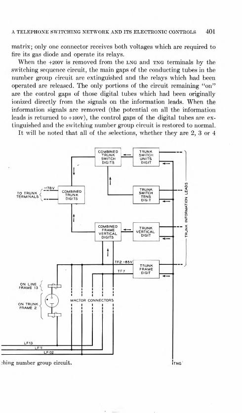
A TELEPHONE SWITCHING NETWORK AND ITS ELECTRONIC CONTROLS 401

matrix; only one connector receives both voltages which are required to fire its gas diode and operate its relays.

When the +200V is removed from the lng and tng terminals by the switching sequence circuit, the main gaps of the conducting tubes in the number group circuit are extinguished and the relays which had been operated are released. The only portions of the circuit remaining "on" are the control gaps of those digital tubes which had been originally ionized directly from the signals on the information leads. When the information signals are removed (the potential on all the information leads is returned to +ioov), the control gaps of the digital tubes are ex- tinguished and the switching number group circuit is restored to normal.

It will be noted that all of the selections, whether they are 2, 3 or 4

, -178 V COMBINED TRUNK DIGITS

ON LINE FRAME 13

ON TRUNK FRAME 2

COMBINED TRUNK SWITCH DIGITS

TRUNK SWITCH UNITS DIGIT

TRUNK SWITCH TENS DIGIT

TRUNK FRAME DIGIT

MACTOR CONNECTORS I I I I I I I I I I I I I I I

LF 03

COMBINED FRAME —■ VERTICAL DIGIT 1

VERTICAL DIGITS

<

;hing number group circuit. TNG

402 THE BELL SYSTEM TECHNICAL JOURNAL, MARCH 1955

digit, are made with nothing more complicated than gas diodes and triodes and reed-contact relays. In general, a selection of one out of any number can be made in this same fashion with the same simple elements, by breaking up the number into groups of digits and combining them in one or more stages as illustrated in the foregoing paragraphs. The gas diodes, triodes, and reed relays which perform the selection can have wide tolerances on their characteristics which means that inexpensive elements can be employed.

Appendix V

POWER SUPPLIES

The power voltages used in the switching network, number group and switching sequence circuits are: —178, —155, —85, —67, —48, —36, -24, -12, +37, +50, +107, +130, +150, and +200. Of these, the —67 volts is obtained by a tap on the — 85-volt supply, the —36, —24, and —12 by taps on the —48-volt supply, and the +37 by a tap on the +50-volt supply. These taps consist simply of resistance divider circuits with an adequate capacitive by-pass to ground. The +150-volt supply is associated only with the generation of an ok or block pulse for trans- mission from the switching sequence circuit to the switching information section of the DIAD. Since the switching information section of the DIAD uses +150 volts also, no separate source is provided on the switching bays. This leaves eight separate power supplies to consider. One of these, the -48-volt supply, is a heavy-duty, regulated rectifier in our laboratory model; however, all of the circuit design has been based on the use of standard -48-volt office battery with limits of 44 to 50 volts. The other seven supplies are small-capacity regulated rectifiers. These supplies are assumed to have a variation in output voltage due to all causes of ±3 per cent. Because of the one-at-a-time nature of the control, the peak load on the power supplies does not in- crease as the size of the office increases, so that the present supplies have sufficient capacity to handle the largest presently used switching net- works. The one exception to this statement occurs in the case of the — 48-volt supply which is used for holding the path operated and to supply talking battery. The loads due to these two functions have peaks which are directly proportional to the number of simultaneous con- versations. It should be mentioned, however, that the holding power for the reed-diode switching network is only one-half watt per path for the four stages.

Signal-Detection Studies, with

Applications

By E. L. KAPLAN

(Manuscript received October 10, 1954)

Curves are given relating the 'probability /3 oj detection of a signal in noise to the signal-to-noise power-ratio S/N, to the proportion a of false detections that can be tolerated, and to the time available {more specifically, to the number m of independent squared samples of the envelope of the filter output that are averaged in making a single attempt at detection). For the curves, three types of sinusoidal signals are assumed, according as the amplitude is constant, varies at random very slowly (fading), or varies as rapidly as the filtered noise itself. The second case is of course very unfavorable for reliable detection, and the third is also if one is limited to one or two sample points. The curves are applied to problems of optimizing radar parameters such as pulse energy, scan rate, averaging time, etc.

The Appendix gives the mathematical background for the foregoing and then proceeds to consider additional types of signal (dc and arbitrary Gaussian) and methods of detection (failure to rectify or take the envelope, counting of samples above a threshold, and averaging by continuous integra- tion) .

1. INTRODUCTION

The word detection suggests a decision between just two alternatives: either a signal was transmitted, or it was not. Typically, however, such decisions are made repeatedly at short intervals of time, with the effect that a multiplicity of possibilities are involved, namely the time intervals in which signals are received, and perhaps also the carrier frequencies at which they are transmitted. In radar and sonar systems, rotating direc- tional receivers map one, two, or three dimensions of space upon the time axis, so that the observation of time is translatable into an observa- tion of position. In these applications, of course, the received signal is a reflection of one transmitted by the observer, and the aircraft or other object to be detected is not attempting to communicate with the ob-

403

404 THE BELL SYSTEM TECHNICAL JOURNAL, MARCH 1955

server. Telegraphy and PCM are applications in which the signals do represent attempts to communicate. In all cases, random noise is present, and will hide signals whose intensity is sufficiently low.

If the bandwidth of the noise accompanying the signal is considerably larger than that of the signal, the best practical procedure is well known to be to pass the signal-plus-noise through a bandpass filter whose band- width approximates the larger of the following: (a) The bandwidth of the signal, (b) The reciprocal of the time available for detecting the signal.1 If the frequency of the signal is not known in advance, one of course moves the pass-band of the filter up and down the frequency scale and thus searches for the signal in frequency as well as in time; the pres- ent discussion applies equally well to this case.

In this way much of the noise may be eliminated, but that is not the end of the problem. Some noise still gets through. However, the presence of a signal may be expected to produce an increase in the magnitude of the rectified output. The purpose of this discussion is to indicate how great this increase should be required to be before one decides a signal is present, to draw conclusions therefrom regarding optimum procedures, and to illustrate the great importance of the nature of the signal and the method of detection. For simplicity, square-law rectification is assumed; it is known that linear rectification does not give very different results.2

The noise, and in some cases the signal also, is assumed to be Gaussian. We assume the following detection procedure, which may apply liter-

ally or else be approximately equivalent to that used in a physical system (e.g., averaging by continuous integration, as in Section 15; or by a human observer, or a phosphor). The rectified output is sampled at m different instants of time,3 which are far enough apart so that the values of the noise are effectively independent (uncorrelated). If the average output at these m instants exceeds the average noise level N by an amount kN or more, we decide that a signal is present; if not, we decide no signal is present. For simplicity, the value of N is assumed to be known as the result of past observation; since this is only approximately true in practice, the results will somewhat exaggerate the effectiveness of the detection procedure, especially for large values of m and low signal strengths. Another assumption made in calculating the curves is that if

1 Alternative (b) is superfluous if, in determining the bandwidth, the signal is defined to be zero outside the time interval within which it is available for analy- sis. . . . 2 M. Schwartz in his Harvard (1951) dissertation, "A Statistical Approach to the Automatic Search Problem," finds agreement to within 0.2 db. 3 This assumes a narrow-band output whose envelope is sampled; if no en- velope is obtained, the number of samples is denoted by 2m. The point will be dis- cussed below.

SIGNAL-DETECTION STUDIES, WITH APPLICATIONS 405

a signal is present at all, it is present at each of the m instants sampled; the methods for removing this assumption are discussed later.

It is well known (and shown in Section 5) that the averaging after rec- tification described above does not fully compensate for a filter whose passband is too wide; but when the filter has been made as selective as it can or should be, the post-rectification averaging, when it is possible, gives a further increase in sensitivity.

In practice many of these averages must be formed, and many deci- sions made, corresponding to the search for the signal in time and possibly also in frequency and in geometrical position (e.g., radar detec- tion of an airplane). The probability (for any one average or any one decision) of deciding that a signal is present is denoted by /3 or a accord- ing as the signal is actually present or not. Thus a is the proportion of false alarms among the total number of averages containing no signal, while (3 is the proportion of valid detections among all those averages that do contain the signal. A detection is considered valid only if it is associated with the average, or one of the averages, in which the signal actually occurs. The average time between decisions divided by a gives the average time between false alarms (in case the signal is usually absent).

The problem could now be formulated thus: to calculate the values of k and (3 corresponding to given values of m, a, and the signal-to-noise power-ratio S/N. Actually it has been convenient to regard m and S/N as the principal variables, and so to plot their relationship for a few different values of (3 and a. The number k depends only on m and a, and is numerically equal to the S/N values {not measured in db) given by the curves for (3 = 0.50 in Fig. 1. (These curves should be rigorously correct for k, whereas their use for S/N involves an approximation as discussed below.)

2. THE THREE TYPES OF SIGNAL AND EXPLANATION OF THE GRAPHS

Three kinds of signal are considered: (1) Steady sinusoid. (2) Fading sinusoid. (3) Noise-like signal. All of these are in a sense special cases, but other signals will generally be of some type intermediate to these.

Cases 1 and 2 are alike in that for both it is assumed that the w signal amplitudes occurring in an average are identical, whereas in Case 3 these m amplitudes are assumed to be independent random variables, just as the corresponding noise values are.

Cases 1 and 2 differ in that in Case 1 the signal-to-noise ratio S/N refers to the instantaneous signal power received, while in Case 2, S/N

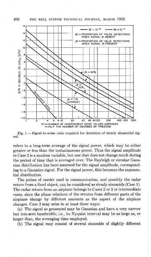
406 THE BELL SYSTEM TECHNICAL JOURNAL, MARCH 1955

A — to-6 A = 10-3

A = PROPORTION OF FALSE DETECTIONS WHEN SIGNAL IS ABSENT

/3 = PROPORTION OF VALID DETECTIONS WHEN SIGNAL IS PRESENT

\

/3 =99%

/3 - 50%

-4 fb = \% v (approx)

-6

Lti -10 4 6 8 10 20 40 60 80100 200 400 600 1000

m = NUMBER OF INDEPENDENT NOISE VALUES AVERAGED = HALF THE NUMBER OF DEGREES OF FREEDOM

Fig. 1 — Signal-to-noise ratio required for detection of steady sinusoidal sig- nal.

refers to a long-term average of the signal power, which may be either greater or less than the instantaneous power. Thus the signal amplitude in Case 2 is a random variable, but one that does not change much during the period of time that is averaged over. The Rayleigh or circular Gaus- sian distribution has been assumed for the signal amplitude, correspond- ing to a Gaussian signal. For the signal power, this becomes the exponen- tial distribution.

The pulses of carrier used in communication, and possibly the radar return from a fixed object, can be considered as steady sinusoids (Case 1). The radar return from an airplane belongs to Cases 2 or 3 or intermediate cases, since the phase relations of the returns from different parts of the airplane change by different amounts as the aspect of the airplane changes. Case 2 may arise in at least three ways:

(a) The signal as generated may be Gaussian and have a very narrow but non-zero bandwidth; i.e., its Nyquist interval may be as large as, or larger than, the averaging time employed.

(b) The signal may consist of several sinusoids of slightly different

SIGNAL-DETECTION STUDIES, WITH APPLICATIONS 407

frequencies beating against one another. If there are reflecting surfaces involved and the source of the signal, the observer, and the reflecting surfaces have any relative motion, the same phenomenon of beats occurs even with a single sinusoid, whenever multiple paths for its transmission exist. Interference between radar reflections from an airplane and from its image in the sea surface is a familiar example.

(c) Even if the signal in each instance is a steady sinusoid, one may still have to regard the collection of amplitudes encountered on different occasions as values of a random variable. Thus, since various airplanes have different speeds and radar cross-sections and are detected at differ- ent ranges, the strengths of their radar returns will differ accordingly. Another example is provided by the interference between direct and reflected signals in the absence of any relative motion among the signal

X v

= 99%

/ /

/ / /

N

4

/ / /

N s X

-N Xj3 = 90% s>-

/ / 'x >

N N •N

"N X

= 50%

r / /

/ /

fs N.

X

\ s., /3 = l%

/ X

X

X \

U — PROPORTION OF FA WHEN SIGNAL IS AE

x^ SENT X

WHEN SIGNAL IS PRESENT 1 1 i i .L I | 1 .J_ 1

, 2 4 6 6 10 20 40 60 80100 200 400 600 1000 m = NUMBER OF INDEPENDENT NOISE VALUES AVERAGED

= HALF THE NUMBER OF DEGREES OF FREEDOM

Fig. 2 — Signal-to-noise ratio required for detection of a fading sinusoidal sig- nal (amplitude steady during each detection, but variable from one detection to another).

408 THE BELL SYSTEM TECHNICAL JOURNAL, MARCH 1955

source, the observer, and the reflecting surface. Then the signal strength may be constant with time, but it will still be a random variable depend- ing on the positions that the source and the observer happen to occupy.

The exponential distribution of signal power assumed in the present treatment of Case 2 is theoretically exact for situation (a) above, and possibly as good as one can do for situation (b). In situation (c) the proper distribution may be quite different, though its effect should be qualita- tively similar.

In all cases the S/N value is defined as if the signal were continuously present; i.e., it does not depend on the duration of the signal. In Case 1, S is the peak signal power, while in Case 2 it is the average of the various possible peak signal powers. In Case 3, S might be described as the peak value of the statistical expectation of the power.

Curves of S/N versus m are given for the three cases in Figs. 1 to 3

\ \ \

o:=io-6 a=io-3

CC = PROPORTION OF FALSE DETECTIONS WHEN SIGNAL IS ABSENT

/3 = PROPORTION OF VALID DETECTIONS WHEN SIGNAL IS PRESENT

\\

w \ \ \ \

\ \ \ s s \ \ \ N \ = 99%

/ X

' Ns /3 =50% x> V

X v.. S

X

/ "x. X /3 =1% >x

X

1 1 1 ^4 1 1 2 4 6 0 10 20 40 60 60100 200 400 600 1000

m = NUMBER OF INDEPENDENT NOISE VALUES AVERAGED = HALF THE NUMBER OF DEGREES OF FREEDOM

Fig. 3 — Signal-to-noise ratio required for detection of a noise-like signal.

SIGNAL-DETECTION STUDIES, WITH APPLICATIONS 409

\ si

\

\ \ S FADING D-C

\ \ \ \v

\ \ \ \

\ \

V \ \

s \

\ \ \

N \

\ \ S. (2) FADING ^sSINUSOID

\ \

\ V NOISE-LIKE \ (SIGNAL ABSENT

\ Sv -N \ IN HALF

\ OF SAMPLES) k \ \

\ ■> \

\ s \

1 i L \ s 1

\ 1 1 1 1

6 6 10 m = NUMBER OF INDEPENDENT NOISE VALUES AVERAGED

= HALF THE NUMBER OF DEGREES OF FREEDOM

Fig. 4 — Comparison of the signal-to-noise ratios required for detecting various kinds of signals.

respectively, for a = 10-3 (dotted lines) and 10~6 (solid lines) and three values of /3. In Fig. 4 one curve from each of the other figures is repro- duced for comparison, and also one new curve (the broken line) to be discussed in Section 6. Curves for /3 = 90 per cent may be interpolated in Figure 1 (and in Fig. 3 when m ^ 10) at about 0.58 of the distance from the curve for d = 50 per cent toward the curve for /3 = 99 per cent. This may be done by eye, or n imerically with S/N expressed in decibels. The curves for /3 = 1 per cent on Figure 1 are probably of low accuracy.

These same three cases are also considered (for somewhat different values of the parameters) by M. Schwartz in his dissertation cited previ- ously, and by J. I. Marcum and P. Swerling in their work at the Rand Corporation.

The curve in the lower left corner of Fig. 1 shows the relation

S/N = 21"" - 1

410 THE BELL SYSTEM TECHNICAL JOURNAL, MARCH 1955

that would exist between S/N and in if the maximum information-carry- ing capacity of the system were utilized. The maximum capacity is (l/2m) bit per Nyquist interval (1/21T; see next Section), achieved by having the signal present with an independent probability of 1/2 in each average of m samples. According to C. E. Shannon's theorem,4 the maxi- mum capacity in terms of S/N is log2(l + S/N)1'2 bits per Nyquist inter- val. When m is large (or equivalently, S/N small), the relation is S/N - (logp2)/m.

3. DETAILS: DC SIGNALS, ENVELOPES, ETC.

This section discusses various other cases of less importance than the three defined in the preceding section; namely, dc signals, low-pass and broadband filters, the relations between instantaneous values and the envelope, and the distinction between narrow-band noise and a noise- modulated carrier. The first three topics are intimately connected; just as sinusoidal (ac) signals, narrow-band filters, and envelopes naturally go together (Sections 1 and 2), so are dc signals, low-pass filters, and instantaneous samples usually associated.

The optimum detection of a dc signal, given independent samples, is trivially easy. No filter is needed, and rectification is undesirable, as shown by the two lowest curves on Fig. 4. The lowest curve, labelled "steady dc," is obtained by the optimum procedure of taking the simple average of the unrectified sample values, some of which may be negative. If the squared values are averaged, the curve will coincide with the next higher curve, labelled "steady sinusoid," as shown later in connection with equations (13b) and (13c). The "fading dc" signal is one which is constant during each detection but has a Gaussian distribution of mean zero from detection to detection. Although it is the worst curve on the figure, quadratic averaging would make it still poorer. [On the other hand, (12c) shows that rectification is as indispensable for the detection of a lowpass noise-like signal as for any other rapidly oscillating signal.] Both of the dc curves are straight lines of 45° inclination, and for them the number of samples is not m but 2m. This adjustment keeps the total time the same, and in the case of quadratic averaging produces complete equivalence between the dc and the sinusoidal signal, as shown in Section 13. The simple formulas applying to the averaging of unrectified dc signals are given later as equations (12a) to (12c).

If a filter is used in detecting a dc signal, it must be of the low-pass 4 B.S.T.J., 27, pp. 379-423, 623-656, 1948. Proc. Inst. Radio Eng. 37, pp. 10-

21, 1949. Mathematical Theory of Communication (with Warren Weaver). Univ. Illinois Press, 1949.

SIGNAL-DETECTION STUDIES, WITH APPLICATIONS 411

type,5 and its effect is not essentially different from that of the assumed averaging of m sample values. In detecting an ac signal, a narrow-band filter is decidedly preferable to a low pass because it eliminates more noise; but it also has the effect of permitting the (squared) envelope of the filter output to be obtained, provided the frequencies contained in this output are confined to a range of less than 3 to 1. In this case the output of the square-law rectifier will contain two separate bands of frequencies of equal widths which (given a reasonable separation between them) can be separated by another filtration. The lower frequency-band is usually the only one that is wanted, and it gives half the square of the envelope of the output of the first filter. If the frequency range of the first filter output is 3 to 1 or more, the envelope is still susceptible of a theoretical definition but it cannot be isolated so easily and is then a somewhat artificial concept.

The general effect of a second filtration after rectification of an ac sig- nal, whether or not the envelope is actually obtained, is to increase the reliability of a single sample, without necessarily having a marked effect on an average over a long (fixed) period of time. The elimination of the sinusoidal component resulting from the signal, and having double its original frequency, is perhaps the main object. If this is not done, it will be necessary to do considerable averaging to eliminate the possibility of missing the signal because of sampling it at its troughs. In this respect instantaneous sampling of a sinusoidal signal is qualitatively similar to the various cases of the sampling of the noise-like signal.

The properties of the envelope will now be considered. Let nfff) and mit) be Gaussian noises containing no radian frequency above u/2. Then the spectrum of

n{t) = nff/) cos 9.1 + ni{t) sin 9t (3a)

is limited to the interval 9 - co/2, 9 + w/2. Conversely, consideration of the Fourier transform of n{t) shows6 that any (stationary) noise whose spectrum is limited to 9 ± co/2 can be expressed in the form (3a). It is found furthermore that

Eni{t)ni(u) = EniiOniiu) = f P(X) cos (X — 9)(t — u) d\ (3b) Jo

Eni(l)no(u) = —Eni(u)no(l) = f P(X) sin (X — 9)(t — u) dX Jo

6 This may not he true in a rigorous sense. If indefinitely prolonged dc signals are not encountered, a cut-off at a sufficiently low frequency is permissible. 6 For example, see S. O. Rice, B.S.T.J., 24, pp. 46-156, 1945, Section 3.7.

412 THE BELL SYSTEM TECHNICAL JOURNAL, MARCH 1955

where P(X) is the power per radian/sec. for frequencies in n{t) whose absolute values are in the neighborhood of X radians/sec. Let yf/o{t — u) and \p\{t — u) represent the two distinct covariances of (3b), the sub- scripts 0 and 1 reflecting the even and the odd characters of the two func- tions. Then

En(t)n{u) = \po(t — u) cos 0,(1 — u) — \pi{t — u) sin — u) (3c)

Replacing in (3a) by fio + gives

n{t) = {ni{t) cos Slit + riiit) sin Slit] cos Slot

+ [ —?ti(0 sin Slit + 712(0 cos ^1^] sin ^ot

so that the same envelope

Vn'iit) + nlit)

is obtained regardless of the value adopted for the "carrier" frequency. However, the highest frequency occurring in ni(t) and 712(0 will be mini- mized by taking SI in the center of band; and (3b) shows that if the power spectrum of n(t) has a center of symmetry which is taken as SI, then Eni(t)ni.{u) = 0.

The noise-like signal used in this study, like the filtered noise itself, has the form (3a). The curves do not apply quantitatively to a single term n\{t) cos Sit obtained by modulating the carrier cos Sit with a low- frequency Gaussian noise-like signal 7ii(0, though the necessary tools are given in equations (13g) and (13h) and the remarks following there- after.

The most obvious difference between the two signals resides in their envelopes, which are

Vni{t) + nl{t)

(with a Rayleigh distribution) and | niit) | (the absolute value of a Gaussian variable) respectively, but other differences may be discovered. The former can be, and is assumed to be, stationary, Gaussian, and ergodic. The latter is stationary only if the phase <p of the carrier cos (fii + ip) is taken to be random, but the relative phases of the sinusoidal components of ni{t) cos {Sit + ip) are still not completely random, and the signal is neither Gaussian nor ergodic. [The Gaussian variable ni{t) is multipled by cos {Sit -j- v), which has the distribution dz/ivs/l — z2.] Where detection is concerned, the two cases are qualitatively similar, but the single term ni{t) cos Sit has a greater amount of fluctuation for the same amount of power, and is therefore a little harder to detect than the sum of the two terms.

SIGNAL-DETECTION STUDIES, WITH APPLICATIONS 413

The results of this study have been phrased in terms of the narrow- band two-term form ni{t) cos Sit + noit) sin Sit for the noise and the noise- like signal. However, the curves apply also to the less important case of the detection of a dc signal by rectification (which is not the optimal procedure, as shown above). The word "sinusoid" is to be replaced by "dc signal," and two independent samples of the rectifier output are to be taken for every one that is prescribed in the narrow-band case. From a noise or signal that (at the input to the square-law rectifier) has a flat spectrum of width W cps, independent samples are obtainable at inter- val \/W seconds in the narrow-band case, and at interval 1/2TF in the lowpass (dc) case,7 so that for large m the averaging time is m/W seconds in both cases. The amplitude of the "fading" signal of Case 2 with its Rayleigh distribution is equivalent in the lowpass case to the RMS value formed from two independent samples of a Gaussian noise-like signal. The case of only one sample could be calculated but would give even less satisfactory detection.

4. NUMERICAL EXAMPLES (RADAR)

The following hypothetical example illustrates the concepts involved. Suppose one has a radar that searches in range and azimuth with a beam 3° wide, a pulse rate of 5,000 per second, a pulse length of 1 microsecond, and a scan rate of 10 per minute. On the average one false detection in 15 minutes can be tolerated. Pulses returned by a target during a single scan arc averaged (after rectification). What signal-to-noise ratio is required to give a probability of 90 per cent of detection in one scan?

This is the narrow-band case. The pulse length is usually about equal to the reciprocal of the bandwidth and so can be taken as the sampling interval. 200 samples of the radar return could then be taken in the 0.0002 sec. elapsing between consecutive transmitted pulses. Suppose that 150 of these arc relevant, giving 150 values of range that can be distinguished. Similarly the azimuth scan of 300° is covered by 120 beam-widths (this does not assume that the azimuth accuracy is no better than 3°). If a factor of 2 is allowed for overlap (in range or azimuth or both) among the averages, the number of decisions per scan is 2 X 120 X 150 = 36,000, or 5,400,000 in a period of 15 minutes. So a = 1/5, 400,000 = 2 X 10"'. In each scan the beam is on a target for 0.05 sec., the time required to turn 3°. In this time 250 pulses are transmitted; this is the value of m,

7 The latter interval is well-known; the former is twice as long because the smoothing accompanying rectification in the narrow-band case makes the sam- pling equivalent to the sampling of tn{l) and no(<), and their bandwidth is not W but only IT/2.

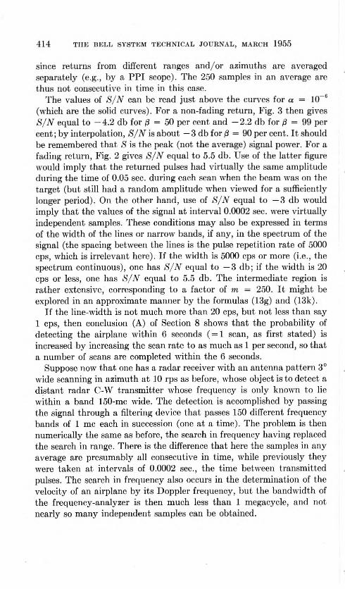
414 THE BELL SYSTEM TECHNICAL JOURNAL, MARCH 1955

since returns from different ranges and/or azimuths are averaged separately (e.g., by a PPI scope). The 250 samples in an average are thus not consecutive in time in this case.

The values of S/N can be read just above the curves for a = 10 h

(which are the solid curves). For a non-fading return, Fig. 3 then gives S/N equal to —4.2 db for = 50 per cent and —2.2 db for /3 = 99 per cent; by interpolation, S/N is about — 3 db for /3 = 90 per cent. It should be remembered that S is the peak (not the average) signal power. For a fading return, Fig. 2 gives S/N equal to 5.5 db. Use of the latter figure would imply that the returned pulses had virtually the same amplitude during the time of 0.05 sec. during each scan when the beam was on the target (but still had a random amplitude when viewed for a sufficiently longer period). On the other hand, use of S/N equal to — 3 db would imply that the values of the signal at interval 0.0002 sec. were virtually independent samples. These conditions may also be expressed in terms of the width of the lines or narrow bands, if any, in the spectrum of the signal (the spacing between the lines is the pulse repetition rate of 5000 cps, which is irrelevant here). If the width is 5000 cps or more (i.e., the spectrum continuous), one has S/N equal to —3 db; if the width is 20 cps or less, one has S/N equal to 5.5 db. The intermediate region is rather extensive, corresponding to a factor of m = 250. It might be explored in an approximate manner by the formulas (13g) and (13k).

If the line-width is not much more than 20 cps, but not less than say 1 cps, then conclusion (A) of Section 8 shows that the probability of detecting the airplane within 6 seconds (=1 scan, as first stated) is increased by increasing the scan rate to as much as 1 per second, so that a number of scans are completed within the 6 seconds.

Suppose now that one has a radar receiver with an antenna pattern 3° wide scanning in azimuth at 10 rps as before, whose object is to detect a distant radar C-W transmitter whose frequency is only known to lie within a band 150-mc wide. The detection is accomplished by passing the signal through a filtering device that passes 150 different frequency bands of 1 mc each in succession (one at a time). The problem is then numerically the same as before, the search in frequency having replaced the search in range. There is the difference that here the samples in any average are presumably all consecutive in time, while previously they were taken at intervals of 0.0002 sec., the time between transmitted pulses. The search in frequency also occurs in the determination of the velocity of an airplane by its Doppler frequency, but the bandwidth of the frequency-analyzer is then much less than 1 megacycle, and not nearly so many independent samples can be obtained.

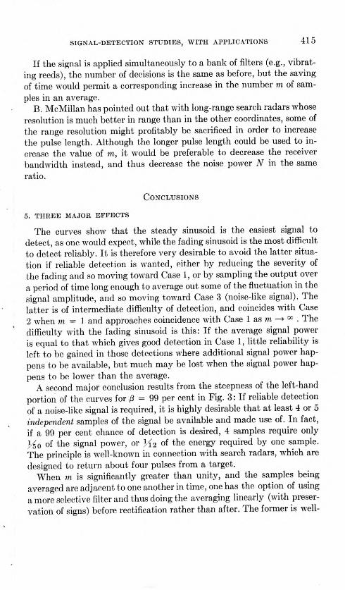
SIGNAL-DETECTION STUDIES, WITH APPLICATIONS 415

If the signal is applied simultaneously to a bank of filters (e.g., vibrat- ing reeds), the number of decisions is the same as before, but the saving of time would permit a corresponding increase in the number m of sam- ples in an average.

B. McMillan has pointed out that with long-range search radars whose resolution is much better in range than in the other coordinates, some of the range resolution might profitably be sacrificed in order to increase the pulse length. Although the longer pulse length could be used to in- crease the value of m, it would be preferable to decrease the receiver bandwidth instead, and thus decrease the noise power N in the same ratio.

Conclusions

5. THREE MAJOR EFFECTS

The curves show that the steady sinusoid is the easiest signal to detect, as one would expect, while the fading sinusoid is the most difficult to detect reliably. It is therefore very desirable to avoid the latter situa- tion if reliable detection is wanted, either by reducing the severity of the fading and so moving toward Case 1, or by sampling the output over a period of time long enough to average out some of the fluctuation in the signal amplitude, and so moving toward Case 3 (noise-like signal). The latter is of intermediate difficulty of detection, and coincides with Case 2 when m = 1 and approaches coincidence with Case 1 as w 00 . The difficulty with the fading sinusoid is this: If the average signal power is equal to that which gives good detection in Case 1, little reliability is left to be gained in those detections where additional signal power hap- pens to be available, but much may be lost when the signal power hap- pens to be lower than the average.

A second major conclusion results from the steepness of the left-hand portion of the curves for /3 = 99 per cent in Fig. 3: If reliable detection of a noise-like signal is required, it is highly desirable that at least 4 or 5 independent samples of the signal be available and made use of. In fact, if a 99 per cent chance of detection is desired, 4 samples require only 1,^0 of the signal power, or K2 of the energy required by one sample. The principle is well-known in connection with search radars, which are designed to return about four pulses from a target.

When m is significantly greater than unity, and the samples being averaged are adjacent to one another in time, one has the option of using a more selective filter and thus doing the averaging linearly (with preser- vation of signs) before rectification rather than after. The former is well-

41G THE BELL SYSTEM TECHNICAL JOURNAL, MARCH 1955

known to be the more effective in Cases 1 and 2. (Case 3, on the con- trary, represents the situation that results when the selectivity of the filter has already been made as great as it can profitably be.) Let the time available for the detection be fixed. Then m, the number of independent noise samples available, is proportional to the filter bandwidth; the latter is inversely proportional to S/N, provided the noise spectrum can be regarded as flat in the region considered, and the filter does not reject any of the signal frequencies. Thus m and S/N are inversely proportional, and one is operating along a 45° line in Figures 1 and 2 (both m and S/N being plotted logarithmically). Evidently 0 is maximized by keeping m (and hence the bandwidth) small.

6. MATCHING THE DURATIONS OF SAMPLE AND SIGNAL

It is fairly obvious intuitively that the chance of detection would be greatest if some one average coincided exactly with the period during which the signal was present. (The signal may be intermittent, as with the first radar of Section 4; if so, the sampling also should be intermittent in the same pattern.) There is no way to insure this if the duration of the signal is not known in advance, but if it is known, the desired coincidence could be approximated to some extent by having the averages overlap; e.g., run from 0 to 1 time unit, to 1 to 2, 1)^ to 2F£, etc. This increase in n necessitates use of a smaller value of a and hence requires an increase in signal strength, but the latter increase is insignificant: When 0 ^ 0.50, the curves show that it is 0.3 db or less for a factor of 2 in a. Similarly, the passbands may overlap when one searches in fre- quency, and the radar antenna patterns may overlap when one searches in direction.

If the averages include fewer samples (though all the samples in some average contain the signal), the effect in any of the Figs. 1 to 4 is to move to the left along a horizontal line. The detection probability 0 is decreased because there is no increase in the concentration of the signal energy, while the fluctuation of the noise is averaged out less effectively.

If the averages include too many samples, then some of these samples will always consist of pure noise, even when a signal is present, and the concentration of the signal energy is reduced relative to that of the noise. If a number m' of samples containing the signal are increased to m by adding m — m' samples of pure noise, the effect in Figs. 1 and 2 is to move down and to the right along a 45° line, since the signal-to-noise ratio is effectively reduced by the same factor m/m' by which the number of samples is increased. Evidently this decreases 0.

SIGNAL-DETECTION STUDIES, WITH APPLICATIONS 417

For the noise-like signal of Fig. 3, new calculations are required when m' < m, and the broken line in Fig. 4 shows some results obtained by the chi-square approximation of equation (13g), with m" = m'. This curve is plotted against m (assumed for this example to be twice m') and so shows the effect of halving the duration of the signal. To show the effect of adding an equal number of pure noise samples (the duration of the signal being kept fixed), the curve should be plotted against m', which is equivalent to moving the curve to the left a distance corresponding to a factor of 2. The resulting curve still lies above the solid curve (for which m = m') for a noise-like signal, but only by about 1 db, which is about

the same loss that one finds in Figs. 1 and 2. It is natural to ask which one should guard against the more, taking

too many samples or too few? The penalty for the former increases rather slowly as we have just seen. The latter is a more serious mistake (espe- cially for the noise-like signal of Fig. 3) if one remains limited to a single opportunity to detect the signal. However, if the signal samples missed by one average are included in another and so give another opportunity for detection, the loss is reduced but not eliminated, as shown below in connection with repeated searches.

7. DISTRIBUTION OF A FIXED AMOUNT OF SIGNAL ENERGY

The preceding discussion is closely related to the question of the op- timum utilization of a fixed amount of signal energy; assuming that m = m', is it better to have a big pulse of signal occurring in only one sample point, or a lower signal power occurring in a proportionately greater number of samples? Here the product of S/N and m is held con- stant, and one moves along a 45° line in all cases, including Case 3. Reference to the curves shows that with a sinusoidal signal one should take m = 1, or at least concentrate the signal energy enough to make the power ratio S/N very much above unity. With a noise-like signal, the same conclusion {in = 1) holds under conditions such that ^ 50 per cent, but when better detection is possible a larger value of m may be preferable. For example, take the solid curves (a = 10 ) in Fig. 3 and suppose that a one-pulse signal makes S/N =18 db. The corresponding 45° line is tangent to the curve /3 = 99 per cent at about m = 15. Thus the maximum detection probability is 99 per cent and is attained by taking S/N = 6.5 db, and so distributing the signal energy among 15 independent samples. Detection with 99 per cent probability by means of a single sample would require 20 times as much energy.

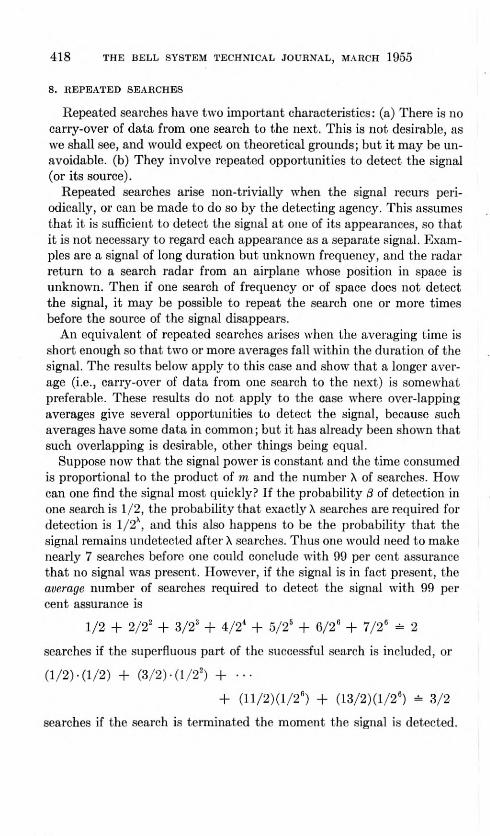
418 THE BELL SYSTEM TECHNICAL JOURNAL, MARCH 1955

8. REPEATED SEARCHES

Repeated searches have two important characteristics: (a) There is no carry-over of data from one search to the next. This is not desirable, as we shall see, and would expect on theoretical grounds; but it may be un- avoidable. (b) They involve repeated opportunities to detect the signal (or its source).

Repeated searches arise non-trivially when the signal recurs peri- odically, or can be made to do so by the detecting agency. This assumes that it is sufficient to detect the signal at one of its appearances, so that it is not necessary to regard each appearance as a separate signal. Exam- ples are a signal of long duration but unknown frequency, and the radar return to a search radar from an airplane whose position in space is unknown. Then if one search of frequency or of space does not detect the signal, it may be possible to repeat the search one or more times before the source of the signal disappears.

An equivalent of repeated searches arises when the averaging time is short enough so that two or more averages fall within the duration of the signal. The results below apply to this case and show that a longer aver- age (i.e., carry-over of data from one search to the next) is somewhat preferable. These results do not apply to the case where over-lapping averages give several opportunities to detect the signal, because such averages have some data in common; but it has already been shown that such overlapping is desirable, other things being equal.

Suppose now that the signal power is constant and the time consumed is proportional to the product of m and the number X of searches. How can one find the signal most quickly? If the probability /3 of detection in one search is 1/2, the probability that exactly X searches are required for detection is 1/2X, and this also happens to be the probability that the signal remains undetected after X searches. Thus one would need to make nearly 7 searches before one could conclude with 99 per cent assurance that no signal was present. However, if the signal is in fact present, the average number of searches required to detect the signal with 99 per cent assurance is

1/2 + 2/22 + 3/23 + 4/24 + 5/25 + 6/2fi + 7/26 = 2

searches if the superfluous part of the successful search is included, or

(1/2)-(1/2) + (3/2) • (1/22) + ..•

+ (ll/2)(l/26) + (13/2)(l/26) = 3/2

searches if the search is terminated the moment the signal is detected.

SIGNAL-DETECTION STUDIES, WITH APPLICATIONS 419

The latter result is the less favorable for repeated searching, since it is 3 times the result {\i) obtained with 99 per cent detection in a single search (which on the average could perhaps be terminated, due to detec- tion of the signal, when it was half completed).

The alternative way of increasing /3 from 50 per cent to 99 per cent is to increase the value of m by a factor lying between 2.3 and 5 for Figs. 1 and 3, while the fading sinusoid of Figure 2 requires a factor of the order of 1,000. Comparing these with the factors 2 (or 3) and 7 obtained previously gives the following conclusions, which have been confirmed by considering some other values of /3:

A. With a fading sinusoidal signal, repeated searching is extremely advantageous, 'provided it is true as assumed that independent samples of the signal are obtainable from search to search but not within a search.

B. Repeated searching may have a small advantage in Cases 1 and 3 (the steady sinusoid and the noise-like signal) provided (1) each search has /3 ^ 50 per cent, and (2) the criterion is the average time required to detect the signal when a signal is present, and one is not concerned with the (increased) time required to conclude that no signal is present (which of course is also the time required for the detection of some of the signals).

G. Repeated searching is somewhat disadvantageous in other cases, as one would expect; e.g., in Cases 1 and 3, if a fixed amount of time is available, the greatest probability of detection is achieved by using all of the time for a single search, rather than dividing it among several less sensitive searches.

Mathematical Appendix

9. PUKE NOISE (AND NOISE-LIKE SIGNAL = CASE 3)

If narrow-band Gaussian noise is applied to a square-law rectifier, the value of the output at any instant has a Rayleigh or exponential distribu- tion, as is well known. The average of m such values, taken far enough apart to be virtually independent has a chi-square (x) distribution with 2m degrees of freedom. The standard form of the distribution used in tables chooses the units so that the mean of the distribution is 2m, whereas we want the mean to equal the noise power N. The exact value of k can therefore be found by means of the relation

Pr(NxL/2m > (k + 1)A0 = « (9a)

or

Pr(xlm > 2m{k + 1)) = a

420 THE BELL SYSTEM TECHNICAL JOURNAL, MARCH 1955

where a. is the expected ratio of false detections to total number of deci- sions, when no signal is actually present.

The usual short tables of x2 (e.g., that in Fisher and Yates' Statistical Tables or that of Hartley and Pearson in Biometrika 37, p. 313) are useful but not entirely adequate for the needs of the problem. The most ex- tensive table is that of K. Pearson,8 which goes to m = 50. In terms of the function I tabulated by Pearson,

Pr(xL > A) = 1 - 7(A/2\/m, m - 1) (9b)

For m > 50 it is sufficient to use the expansion9

xlm = 2m + 2umm + %{u2 - 1) + Hsiu - 7u)m~112 - • • • (9c)

Here u is the standard normal10 deviate. Thus if ua is defined by

a = Pr{u > ua) = f e-"2/2 dw/V^TT ^ ua

one has

k = Ua/y/m + («a — l)/3m + • • • (9d)

If a noise-like signal is present, this is mathematically the same as an increase in the average noise power from N to N + S, the critical power level remaining at (k + 1) N. The probability of exceeding the critical level is now the probability 13 of a true detection. Thus

(3 = Pr[(N + S)xL/2m > (k + \)N\ (9e)

= Pr[xL > 2m(k +!)/(! + S/N)]

Writing xim(l3) for the number that is exceeded by the variable xlm with probability 0, one gets from (9a) and (9e)

1 + S/N = xU«)/xL(/3) (9f)

For large m (and only in that case), (9c) then gives

, , f 1 Ua — 2up~\ S/N * in. - uf) + -^J ( g)

8 K. Pearson, Tables of the Incomplete Gamma-Function, Biometrika Office, London, 1934. 0 The author first discovered this formula in T. Lewis, Biometrika 40, p. 424, 1953; but S. O. Rice has pointed out that G. A. Campbell published it as early as 1923 in the B.S.T.J., 2, page 95, in connection with Poisson distribution. Other references and inversion formulas are given by John Riordan. Ann. Math. Stat., 20, p. 417, 1949.

ic "Normal" is a synonym for "Gaussian." However a new application of the distribution is involved here, and so there is no disadvantage in making the con- ventional change in terminology.

SIGNAL-DETECTION STUDIES, WITH APPLICATIONS 421

where the standard normal deviate Up is defined by (3 = Pr(u > Up). It is negative when /3 > 50 per cent.

Wherever it occurs in equations, S/N naturally means the ratio of S to N, and not the value in db, which is 10 logio S/N.

10. NOISE PLUS STEADY SINUSOID (CASE l)

When a pure sinusoidal signal of constant amplitude is added to the noise, the distribution of the rectifier output has what is called a non- central chi-square distribution, which has been little tabulated. For- tunately the normal distribution gives a fair approximation in this case (with the probable exception of small values of 0, which are of little interest anyway). More accuracy could be obtained at the cost of addi- tional labor.11

Before rectification, the signal plus noise can be represented, as re- marked in Section 3, by the expression

■\/2S cos (SM + v?) + ni(t) cos (fi/ -f (^) + no(t) sin (12/ -f tp) (10a)

where the two Gaussian noise variables wi(/) and no(/) are independent and have zero means and a common variance N. After rectification and smoothing, half the square of the envelope is obtained, namely

Its mean value is N + S, and its variance is the sum of the variances of the terms in the expanded form, namely 0 + 2NS -f N'/2 + N2/2 or 2NS + N2. The average of m such independent variables has the same mean N -f S but the variance N(N -f 2S)/m.

The critical value (A: + l)iV of the rectifier output is reduced to stand- ard units by subtracting the mean output N -f S and dividing by the square root of the variance, giving

by using a table of the normal distribution, one can solve the preceding

11 P. B. Patnaik, Biometrika 36, p. 202, 1949.

[(\/2S + Wi(/))" + ni(t)']/2

After Up is found from

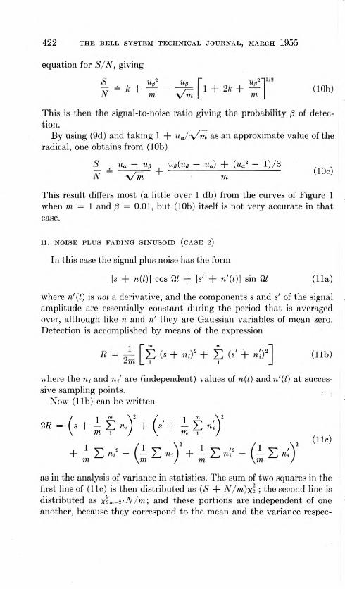
422 THE BELL SYSTEM TECHNICAL JOURNAL, MARCH 1955

equation for S/N, giving

« ,+ v %(" +«q"!

N m v m L m J

This is then the signal-to-noise ratio giving the probability 13 of detec- tion.

By using (9d) and taking 1 + ujy/m as an approximate value of the radical, one obtains from (10b)

8 Ua — Ug UffiUff — Ua) + (lla2 — l)/3 — — /— + (10c) IV v m m

This result differs most (a little over 1 db) from the curves of Figure 1 when m = 1 and $ = 0.01, but (10b) itself is not very accurate in that case.

11. NOISE PLUS FADING SINUSOID (CASE 2)

In this case the signal plus noise has the form

[s -f «(/)] cos Vll + [s' + n'{t)] sin Vll (Ha)

where n'{t) is not a derivative, and the components s and s' of the signal amplitude are essentially constant during the period that is averaged over, although like n and n' they are Gaussian variables of mean zero. Detection is accomplished by means of the expression

^ = 2~ (s + w,)2 + 53 (s' + Wi)2J (lib)

where the n,- and n/ are (independent) values of n(t) and n'(l) at succes- sive sampling points.

Now (lib) can be written

2R=(s+±t n,y +(s'+±± n'tY \ m 1 / \ m 1 /

+ 1 Z n.2 - (i Z n.Y + - E n? - Z m \m / m \m /

as in the analysis of variance in statistics. The sum of two squares in the first line of (11c) is then distributed as (S N/m)xi ; the second line is distributed as xlm-i -N/m\ and these portions are independent of one another, because they correspond to the mean and the variance respec-

SIGNAL-DETECTION STUDIES, WITH APPLICATIONS "423

tively of the sample of n,- (or n'i), and the sample mean and variance are known to be independent in the Gaussian case. Here the signal power S is the variance of each of s and s', and N is the variance of each of the iii and rii .

For detection R must exceed ^(1 + k). Hence if S/N is denoted by r, one has

d = Pr[(l + mr)x2 + xL-a > 2m(l + k)] (Ud)

Since (1 + mr)xl has the c.d.f. 1 - e-"w+",r) and xL-s has the density

function

e-"hm-2/2m-1T(m - 1),

/3 is obtained by convolution as

/3 = 1 — f [1 - e-(!-t),m+mr)]e-t,2tm-2dt/2m-lT{m - l) Jo

= Pr[x2m-2 > 2] + (He)

^ mrz 1 + mr ]

where z = 2m (1 + k). An excellent approximation is obtained by replacing the variable

X2m—a by its mean value 2m — 2; this is reasonable, since the ratio of the variances of xlL-a and (1 + mr)x2 is (m — 1)/(1 + m S/N)2, which is very small throughout the interesting area f/3 ^ 50 per cent), (lid) then gives

/3 = exp [-(1 + km)/(1 + m S/N)] (llf)

This result will be generalized in (13k) below. Using (9d) then gives

S . Ma , {uj + 2)/3 - fn (m - (n (1//3) = -7= + (Ug) N v m m

to a little lower order of accuracy when m is small, and still with ft ^ 50 per cent.

Before the foregoing results were obtained, the curves ot Fig. 2 had already been calculated12 on IBM equipment by the rather tedious proc- ess of integrating the results for Case 1 with respect to the random signal

12 By Mrs. L. R. Lee, at the request of the author.

424 THE BELL SYSTEM TECHNICAL JOURNAL, MARCH 1955

strength. This gives

p = [ $[(xS/N - AO Vm/(1 + 2xS/N)]p(x) dx (llh) Jo

for Case 2, where ■p{x) = e~r

and

^(w) = f e '2/2 di/■\/2ir ^ CO

If the fading is due to interference between two sinusoidal signals of powers Si and ^(aSi + -SO = S) and very slightly different frequencies, it can be shown that the appropriate form for p(a;) is I/tuv/A2 — (1 — x)2

for 1 — A < a: < 1 + A, and zero elsewhere, where A = 2\/SiS-i/ {Si + ^2). Here x can approach zero only in the special case Si = S2. Since one or both of Si and S2, and hence A, is likely to be a random variable, one apparently cannot say a priori that any particular dis- tribution p{x) is the appropriate one in this case.

12. COMPARISON OF 12 CASES

The three principal cases defined in Section 2 and analyzed in the last three sections may be expanded to 12 by considering dc signals as well as ac, and considering also a second method of detection. The original 3 cases will be labeled "ac envelope." (More precisely, half of its square is the quantity averaged.) If the envelope is not isolated but instantaneous squared values are sampled, the situation is "ac instantaneous." A pre- cise analysis of these latter cases would apparently be difficult. As indi- cated, quadratic rectification is assumed for all 6 of the ac cases. On the other hand, for the 6 dc cases, distinguished as rectified and unrectified, it is the instantaneous sampling that is assumed throughout.

The reduction of the rectified dc cases to the standard ac envelope cases has been indicated at the end of Section 3, and will be demonstrated at the beginning of the following section. The unrectified dc cases, which represent the better way to detect a steady or fading dc signal, involve nothing but the simple Gaussian distributions specified in Table I. If the number of samples averaged is denoted by 2m, one easily finds the the- oretically exact relations

S/N = (iia — up)2/2m

S/N = (ulv/uln - l)/2m

S/N = u'cn/upii - 1

(12a)

(12b)

(12c)

SIGNAL-DETECTION STUDIES, WITH APPLICATIONS 425

Table I — Variables to be Averaged

DC Unrectified DC Rectified

Steady... Fading Noise-likeJ

Steady... Fading Noise-like

Steady... Fading . . Noise-like

VS + n s -f n

S + 2n VS + n2

s2 + 2ns + n2

AC Envelope

S + n \/2S + (n* + n'2)/2 [{s + n)2 + (s' + n')2l/2

AC Instantaneous

[(VSS + n) cos v -f n' sin <p]2

[(s + «) cos v' + (s' T «') sin v']2

Ditto or s2 -1- 2ns + n2

for the steady, fading, and noise-like imrectified dc (or low-pass) signals. As usual, Up is defined by

f dl/s/'Itt = p Jup

In (12a) it is assumed that the steady dc signal of magnitude \/S is of known sign. Otherwise it would be necessary, as with fading and noise-like signals, to be prepared to detect both positive and negative dc signals, and quantities like ua/o enter in place of ua via the relation

/CO z*-"a/2

+ L =a-

As 0 approaches unity, i%2 approaches zero and S/N rapidly approaches infinity for the fading and the noise-like signal. In the latter case (12c), averaging has no effect (m does not appear), because the imrectified signal averages to zero as fast as the noise does. In fact, with instantaneous sampling of a noise-like signal, there is no essential difference between the lowpass ("dc") and narrow-band (ac) cases.

If n, n', s, s' are independent Gaussian variables with zero means and variances N, N, S, S respectively, and <p is uniformly distributed between 0 and 2ir, the variables that are averaged in the detection process have the forms given in Table I in the various cases, when a signal is present (if not, put s, s', and S equal to zero).

Table II gives the variances of the variables of Table I for the cases

426 THE BELL SYSTEM TECHNICAL JOURNAL, MARCH 1955

Table II — Variances

DC Unrectified DC Rectified

Steady Noise-like

Steady Noise-like

N N + S

2N2 + 4NS 2N2 + 4iVS + 2S2

AC Envelope AC Instantaneous

N2 + 2NS N2 + 2NS + S2 2N2 + 4ArS -|- tfS2

2N2 + INS + 2S2

of a steady or a noise-like signal. The means are and zero, respec- tively, for the dc unrectified variables, while all the others have the power iV + $ as their mean.

Table III gives the data for the fading signal. The reducible variance and the mean are calculated under the condition that s and s' are fixed; the irreducible variance is then the variance of the resulting mean when s and s' do vary. The distinction between the two variances is that by averaging, the first is reduced in the usual way (divided by the number of samples), while the second retains its full value. The variance already given for the steady signal can be derived from the reducible variances above by replacing s2 and .s'2 by S. The variances already given for the noise-like signal are equal to the irreducible variance plus the expected value of the reducible variance.

The steady ac instantaneous case will serve to illustrate the calculation of the variance. If the rectifier output is written in the form

S + n\/2S + (n + n'2)/2 + (w'\/2>S + nn') sin 2.?

+ [S + ns/:2S + {n — n'2)/2] cos 2^

it may be verified that the various terms are uncorrelated with one another, so that their individual variances may be added. Also E sin 2<p = E cos 2<p = 0, E sin2 2^ = E cos2 2<p = 3-^, En* = En'* = 3N',

Table III — Fading Signals

Reducible Variance Mean Irreducible Variance

DC unrectified DC rectified AC envelope AC instantaneous ...

N 2N2 + 4A's2

N2 + N (s2 + s'2) 2N2 + 2Ar (s2 -1- s'2) +

(s2 + s'2)2/8

s A" + s2

N + (s2 + s'2)/2 N + (s2 + s'2)/2

S 2S2

S2

S2

SIGNAL-DETECTION STUDIES, WITH APPLICATIONS 427

var n' = var n'~ = 2N'. These last relations are not obvious, but are a special case {I = u) of the relation cited below just prior to (15e). The variance is now obtained as

0 + 2NS + AN'/A + \^E(2Sri' + nn'-)

+ MEAS2 + 2Sn- + {n - 2n n'2 + n,4)/4]

= 2N0- -f ANS + S2/2

The variances tabulated indicate the relative merit of the various cases. If m is significantly greater than unity, the anomalous case of an unrecti- fied noise-like signal represented by (12c) gives the poorest detection; next come the fading signals with their irreducible variances. The steady dc unrectified signal with S/N proportional to m 1 (by 12a) is the easiest to detect. The steady signals are in all cases more easily detected than the noise-like at the higher signal strengths. However, instantaneous sampling of a steady ac signal loses some of this advantage; a term S2/2 appears, in addition to the expected doubling of the variance of a single sample.

13. DETECTION OF AN ARBITRARY GAUSSIAN SIGNAL

General formulas will now be derived which include Cases 1, 2, and 3 and also give approximations to intermediate cases. It will be more con- venient to deal with the Gaussian sample values s, + n,- of the signal plus noise in the dc or lowpass case, and 2m of them will be taken so that the results obtained will have the same form as those already given for the ac or narrow-band case. Detection is then accomplished by means of the variable

2 m 2 m /? = 2 (s' + n,)2/2m = X] (s.-2 + 2s,n,- + nr)/2m (13a) i i

It is assumed that the n, are independent of one another and of the s,-, while the s,- may be constant or mutually correlated. Also Erii = 0 and En2 = N, a constant.

An orthogonal transformation (rotation in 2m-dimensional space) can be used to show that (13a) has the same distribution as

£ {h + n/)72m (13b) i

or

£ (/i \/2 + n")' + £ w, 1 m+l

2m (13c)

428 THE BELL SYSTEM TECHNICAL JOURNAL, MARCH 1955

where h' = y.i"1 sf /2m, and the n/ or n" are new noise variables with exactly the same properties as the original n, . Evidently h2 is so defined as to leav^e unchanged the terms independent of the noise variables, while the orthogonal transformation by definition makes ^ nr = S ni ' = ^ n/'-. Thus it is only necessary to choose the transformation so that the original linear terms y.?'" sim/m go into h y.?"' n//m or \/2h "Y/" n"/m. This is always possible since all three expressions have the same norm (square root of sum of squares of coefficients), namely h \/2/m.

The forms (13b) and (13c) are appropriate to the instantaneous sam- pling of the square of a dc signal plus noise, and the sampling of the square of the envelope of an ac signal plus narrow-band noise, respec- tively, the latter being the standard case. Thus the equivalence (f the two cases is established. It is only necessary to observe that the number of samples taken is 2m in (13b) but only m in (13c). The noise powers are En/ and

E(ni cos (p + nm+i sin (p)2 = E(n/ + n,;l+t-)/2 = En/.

The signal powers are h' and E■ 2}i cosV = h2. Another consequence of (13b) or (13c) is that when the distribution of h has a known form, the distribution of R could be obtained from the results for Case 1 by inte- grating over h, as stated at the end of Section 11.

The mean and the variance of the general form (13a) will now be cal- culated. It is assumed that Es, = 0 and Es/ = S for the first 2m' values of i{m' ^ m), while s,- = 0 for the other 2(m — m') values of i. Then one has ER = N -\- m'S/m. If i and j are any two distinct integers, the five variables s/, s.n, , SjUj, n/, nf are all uncorrelated (though not all inde- pendent), and so one has

4m2 var R = var (Y */) + d ^ var (s.n.) + 2m var n/

Since var (s.-n.) = NS or 0 and var n/ = 2N2, this gives

var R = var h2 + 2m'NS/m2 + N2/m (13d)

with h1 = y.2"" s//2m. In Cases 1, 2, and 3, var h2 = 0, (m'S/m)2, and m'S2/m2 respectively. (In Case 2, m' of the s, have one identical value and m' have another identical value, independent of the first.) In general

var h2 = y (2m' — \i\)\p2(i)/2m2 (13e) —2m'+l

where \f/(i) = EsjSi+j for all j for which syst+y ^ 0. This is the discrete analogue of the integral appearing in (lo/o) below. It is convenient to define a number m" (which need not be an integer) such that var h2 =

SIGNAL-DETECTION STUDIES, WITH APPLICATIONS 429

{m! S/mf/m". Then putting S' = m'S/m gives

ER = N + S', var R = S,2/m" + (2NS' + N2)/m. (13f)

The mean and variance of R are identical with those of [S'2/m" + (2NS' + N2)/m]/2(N -f- S') times a chi-scjuare variable with

2m = 2{N + S'f/[S,2/m" + {2NS' -f N2)/m]

degrees of freedom. So one has approximately

0 = Pr(R > (k + 1)N)

= Pr[x\m > 2(k + 1)N(N + S,)/[S'2/m" + (2NS' + N2)/m]} (13g)

= Pr{u> (kN - S')/VS'2/m" + (2^' + N2)/m\

The last line can be used to verify that for fixed m, the optimum value of m' is m, and for fixed in', the optimum value of m is m'. Defining up by Pr(u > up) = 0 and solving for S/N = mS'/m'N gives

S/N

ink + up2 — up \/(2/c + I)in + — ufjm/m" — m'(l — up-/in")

The approximation breaks down if up2 ^ m". It can be shown that by replacing the symbols in', m", and £ in the

above formulas by m' 12, m" 12, and 28, one obtains the results for the narrow-band case in which the signal is a noise-modulated carrier s(t) cos til, while the noise as usual has the form n(t) cos fit + n'(t) sin fit.

In Cases 1, 2, and 3, w" = 00 , 1, and in' respectively; also, m' has been assumed equal to in. In the dc or lowpass case, m" could be as small as 3/2- One has m ^ m' always, and in' ^ in" when the signal is Gaussian (i.e., contains no steady sinusoidal or steady dc component).

When 111" is very small, (13g) and (13h) are of low accuracy, and it is much better to use (lie) or (Uf), or the following generalization of them. The derivation proceeds as if m'/m" were an integer, although this is probably not a necessary condition for the usefulness of the results. The averaged rectifier output is represented by

2m" m'/m" 2m—2m' 2mR = 2 £ (si + n.-y)2 -f £ n,-2 (13i)

<=1 y=i i

where the w.-y are 2m' independent Gaussian noise variables accompany- ing the signal variables s,- (which have only 2m" independent values), and the n,- are 2m — 2m' additional noise variables that are not accom-

430 THE BELL SYSTEM TECHNICAL JOURNAL, MARCH 1955

panied by a signal. Of course, the signal variables would not in reality fall into independent sets of identical values, so that an approximation enters here even if m'/m" is an integer.

(13f) may be written as 2m" 2m" m-/m"

2mR = (m'/m") X (s.- + Wf+)2 + £ 2 (^0 — >=1 j=i j=i

+ 2 ^ = (iV + m'S/m")x2m" + Nx2m-2m" 1

where m'/m''

fii+ = {in"/m') X! na 3=1

S = var Si

N = var Uij = var w,-

and the two x' variables are independent. If the ratio m"{m — m")/ (in" + m'S/Nf of the variances of the latter (including their multipliers) is small, one may replace X2m-2m" by its mean value 2m — 2m" and ob- tain

iS - Pr[R > (1 + h)N\ (13k)

= Pr[xL" > 2(m" + ink)/(1 + m'S/m"N)]

14. COUNTING SAMPLES ABOVE A THRESHOLD

It is sometimes suggested that instead of averaging the m samples, the number of such samples exceeding some threshold might be counted and used as the detection criterion. This is equivalent to replacing the average of the m samples by one of their order statistics, such as the median.

It is of interest to ask which order statistic is best to use, and how it compares in efficiency with the average. M. Schwartz (in the dissertation cited previously) made numerical calculations for the case of a steady sinusoid and in ^ 49, and concluded that the method of coincidences, as he called it, required S/N to be about 1.4 db above that which sufficed for equal performance using averages. For the larger values of m there appeared to be a small advantage in requiring less than half the samples to exceed the (suitably chosen) threshold. These results are confirmed by the following asymptotic analysis.

In the absence of a signal, a single sample of half the square of the

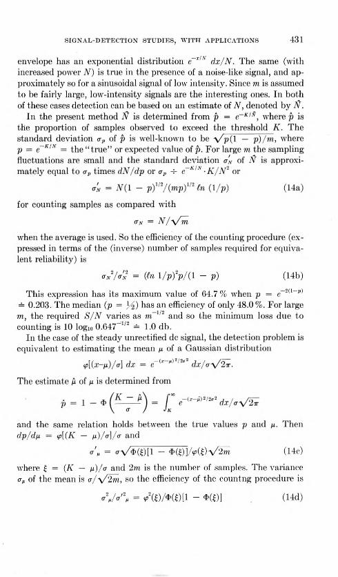
SIGNAL-DETECTION STUDIES, WITH APPLICATIONS 431

envelope has an exponential distribution e_x/A dx/N. The same (with increased power N) is true in the presence of a noise-like signal, and ap- proximately so for a sinusoidal signal of low intensity. Since m is assumed to be fairly large, low-intensity signals are the interesting ones. In both of these cases detection can be based on an estimate of N, denoted by N.

In the present method N is determined from p = e~KlN, where p is the proportion of samples observed to exceed the threshold K. The standard deviation <tp of p is well-known to be \/p(l — p)/m, where p = e~KIN = the "true" or expected value of p. For large m the sampling fluctuations are small and the standard deviation a'N of N is approxi- mately equal to o-p times dN/dp or <tp -h e~K,s -K/N' or

(r'N = A^(l - p)1'2/{mpf12 In (1/p) (14a)

for counting samples as compared with

(T,v = N/y/m

when the average is used. So the efficiency of the counting procedure (ex- pressed in terms of the (inverse) number of samples required for equiva- lent reliability) is

on/o'n = {fn l/p)lp/{\ - p) (14b)

This expression has its maximum value of 64.7 % when p = e-"2(1_p)

= 0.203. The median (p = j 2) has an efficiency of only 48.0%. For large m, the required S/N varies as m-1'2 and so the minimum loss due to counting is 10 logio O.G47~'/' — 1.0 db.

In the case of the steady unrectified dc signal, the detection problem is equivalent to estimating the mean ^ of a Gaussian distribution

(p[{x—p)/a\ dx = e (l dx/ay/'Iir.

The estimate A of /i is determined from

p = 1 - * e~(T~,1)2l2al dx/ay/^

and the same relation holds between the true values p and n- Then dp/dp = <p[{K — p)/(j\/(j and

o-'p = o-v/l5^)!! — <t>{£)]/(p(0\/2m (14c)

where ^ = (K — p)/<j and 2m is the number of samples. The variance o-p of the mean is a/y/'Zm, so the efficiency of the countng procedure is

c\/<r'\ = Ao/Hm - m]

432 THE HELL SYSTEM TECHNICAL JOURNAL, MARCH 1955

The following are some values of this expression:

^ 0 0.5 1 2 Efficiency 63.7% 58.0% 43.9% 13.1%

Thus the highest efficiency of 63.7 % is attained when £ = 0 or the threshold K equals the mean n- This corresponds to using the median as the statistic on which detection is based. This maximum efficiency is very nearly the same as that obtained in the preceding case. However, in the present case S/N varies as m-1 by (12a), so that the equivalent loss in signal strength is not 1.0 but 10 logic 1/0.637 — 2.0 db.

15. AVERAGING BY CONTINUOUS INTEGRATION

In practice, in place of the discrete sums of squares such as (lib) and (13a) one may have integrals such as

Ra = [ Z{t) dt/T and (15a) Jo

Re = f Z(t)etlT dt/T (15b) CO

where Z{t) is the variable to be averaged (usually a rectifier output), and the subscripts U and E refer to uniform and exponential weighting respectively. The purpose of this section is to calculate the mean /i and variance a'1 of each of these expressions for various cases. It will then be shown that for a flat spectrum and T —* <*>, n and cr2 are the same as those already given for the discrete averages of samples. The results are closely related to those given by Rice.13

It will suffice to consider steady signals. If the signal is absent, put S = 0. If the signal is fading, 5 is a random variable. If the signal is noise-like (with the same spectrum as the noise), put S = 0 and replace iV by iV + »S. The four combinations of ac and dc signals with two methods of detection (see Section 12) will be considered separately.

The exceptional case of an unrectified dc signal may be disposed of first. Then Z(t) = \/S + n(t) and Ru and Re both have Gaussian dis- tributions with mean \/S. The variance of is

E^nit) dt/fj

Writing the square as a double integral and taking the expectation under

13 S. O. Rice, B.S.T.J., 24, pp. 46-156, 1945, Eqns. 3.9-8 and 3.9-28. Also J. Acous. Soc. of Amer., 14, pp. 216-227,1943.

SIGNAL-DETECTION STUDIES, WITH APPLICATIONS 433

the integral sign gives

nr n(t)n(u) dt du/T2

fT *T .T (15c) = / / - u) dt du/T2 = 2 (T — v)t{v) dv/T2

Jo Jo Jo

where ^(v) = En(t)n(t + v), and ^(0) = N. Similarly

var Re = f0 r e-('+u)lTt(t - u) dt du/T2

Jo Jo dod)

= / e-vlTt{v) dv/T Jo

In the remaining three cases, Ru and Re always have the power N + S as their mean. Their distributions are not known exactly but they might be assumed to be distributed approximately like (o-2/2/x)x22M2/.r2

where u is the mean N + S and a2 is the appropriate variance given below. A probably more convenient procedure is to use the m = A" and a1 = o-q2 (see 15k and f) for the noise alone to determine an equivalent value N2/<to for m, and then use Figs. 1-3.

Consider next the rectified dc signal, so that

Z{t) = S + 2VSn(t) + n2(t)

The variance of i??/ is E[Ru — S — A]2 or

UT T \ 2 [nit) - A] dt/T + 2\/S fQ nit) dt/Tj ,

The cross-product has zero expectation. Expressing the squares as double integrals gives

E [T fT i[n2it) - N][n2in) - A] + 45n(0n(w)) dtdu/T2. Jo Jo

We now take the expectation under the integral sign. For

En2it)n2iu) = ^(O) -(- 2\f/'it — u)

see M. G. Kendall, The Advanced Theory of Statistics, Volume I, Sec- tion 3.28, equation

M22 = (1 + 2p')oT(T2'

434 THE BELL SYSTEM TECHNICAL JOURNAL, MARCH 1955

This gives

var Ru = [ [ — u) + 4S\p{t — ii)] dtdu/T2

Jo Jot (15e)

= 4 f (T - v)[t2(v) + 2St(v)J dv/T2

Jo

A similar treatment of R# gives

var R, = 2 [' e-'VW + 2Sf{v)] dv/T. (15t) Jo

The third ease is that of a sinusoidal signal with instantaneous sam- pling, for which

Z(t) = 2S cos2 (nt + ^) + 2y/2Sn(t) cos {Qt + ^) + n(t)

where ip is uniformly distributed in (0, 2t). The variance of Ru is now given by

E * \n\t) - A^J dl/T + 2 ^ s/28 cos + <p)n{t) dt/T

+ J »S[2 cos2 (iit + v3) — 1] dt/Tj

= E fTfr [n2{t) - M[nV) - N] dtdu/T2

Jo Jo nT

cos (fit + <p) cos (flu + <p)n(t)ii(u) dt du/T

nT

cos (2Qt + 2tp) cos (2flu + 2tp) dtdu/T2

To find E cos (fit + ip) cos (fiu + ip), expand the cosines, note that E cos2 ip = E sin2 f = H and E cos ip sin ^ = 0, and combine the re- sulting terms. This gives

var Ru — f [ (2ip2(t ~~ u) T 4S\f/(l — u) cos ffi(l — u) Jo Jo

+ >^S2 cos 2Sl(t - u)) dt du/T2 (15g)

= 4 fT (T - v)lt2(v) + 2St(v) cos Qv] dv/T2 + (S2/2T2fl2) sin2 flT. Jo

SIGNAL-DETECTION STUDIES, WITH APPLICATIONS 435

A similar treatment of Re gives

var Re =

/•« (I oh) 2 / e~v [\l/'{v) + 2S^{v) eos fiy] dv/T + £72(1 -f 4T2«2)

Jo

of which the last term is the evaluation of

s r r e-(,+u),T cos 2^t _ dt du/To 2 Jo Jo

It remains to consider the narrow-band case, with filtering after rectification to give half the square of the envelope. As in Sections 3 and 10, the final output has the form

Z(t) = £ + ■\/2Sni(t) -f [wi"(/) -f W2"(f)]/2

The variance of Ru is then

E Q f* [n^/) + nlil) - 2N] dt/T + V2S f* n,(0 dt/lj

The usual method of evaluation gives

var Ru = 2 [ (T - v)[tl{v) + tl(v) + 2£^o(c)] dv/T2 (15i) Jo

var Re = f e_,'/r[^o(y) + tiiv) + 2S\//o(v)] dv/T (15j) Jo

where

^o(y) = Eni(t)ni(t + v) = Enzityriiit + v) and

\pi{v) = Eni(t)ni{t + y) = — Eni{t +

Then 7' 00 , the ratio of the variances oi Re and Ru approaches one-half in all cases, so it will suffice to consider the latter. The spec- trum of the noise will be assumed to be flat, of width w radians per sec- ond. Then in (15c) and (15e) one has ^(y) = N sin uv/uv, and so the variance of Ru is asymptotically equal to

2 1"° N sin coy If 1 Jo coy

dv

and

respectively.

fi'D N' sin2 coy 2NS sin coy

(coy)2 coy dv

436 THE BELL SYSTEM TECHNICAL JOURNAL, MARCH 1955

Putting \P(v) = (2N/uv) sin (coy/2) cos Slv in (15g) gives

4 f" [-jV2 sin2 fartj/2 + 2iVasmM/2-| ^ T Jo L (coy/2)2 coy/2 J

Putting

Mv) = 0. ^o(y) = (2N/coy) sin (coy/2) in (15i) gives

2 r" f ^y2 sin2 coy/2 2^5 sin coy/2"| W i

TJo L (coy/2)2 coy/2 J

The first integral has the value ttN/uT and the last three all have the value (27r/coT)(iV'" + 2NS). Comparing these with the variances of single samples given for steady signals in Table II (Section 12), and writ- ing co/27r = W cps we see that Ru is asymptotically equivalent to 2WT independent samples in the two dc cases, and WT in the ac envelope case. The number is something above 2WT for instantaneous samples of ac. These results agree with those arrived at in Section 3 and 13. With the exception of the unrectified dc signal, the differences are seen to lie in the efficacy of an isolated sample, rather than in the long-term rate of transport of information.

When the signal is absent, (15e) to (15h) reduce to the results of Rice cited above:

var Ru == 4 fT (T — v)t\v) du/r (15k) Jo

and

var = 2 f e-'VW dv/T (150 Jo

The same is nearly true for (15i) and (15j) also, since by (3c), ^l(v) + rpl(v) is the square of the envelope of \p'2(v) in the narrow-band (ac) case.

16. OPTIMUM PROCEDURES AND THE BASIC ASSUMPTIONS

The rigorous determination of the optimum detection procedure is a deep problem with more or less complicated answers depending on the spectra and probably involving both discrete sampling and continuous integration, or even differentiation.1416 However, the solution of the prob-

14 U. Grenander, Stochastic Processes and Statistical Inference, Arkiv for Matematik, 1, p. 195, 1950, Sections 4.11 and 5.4. AT .

16 E Reich and P. Swerling, The Detection of a Sine Wave in Gaussian Noise. J. Appi. Phys., 24, p. 289, 1953. . ^ . xr ■ ^ 16 D. Slepian, Estimation of Signal Parameters in the Presence of Noise, trans. I.R.E., Professional Group on Information Theory, p. 68, March, 1954.

SIGNAL-DETECTION STUDIES, WITH APPLICATIONS 437

lem is known as soon as one restricts oneself to independent samples of the signal-plus-noise. Then square-law detection and averaging is the rigorously optimal procedure for detecting a noise-like signal, and it is virtually optimal for a steady sinusoid. The rigorous optimum in the latter case is well-known and depends on the assumed signal power S] if y is the amplitude of the envelope (output of a linear rectifier), then a non-linear rectifier or other device is to be used to convert v to log Io(vV2S/N), and the values of the latter are averaged. 7o(a:) is the Bessel function Jo(x V — 1). This corresponds very nearly to square-law rectification when S/N is small, and linear rectification when S/N is large. Since square-law is little different from linear rectifi- cation, as noted in Section 1, it is also little different from the optimal. For a steady dc signal, the optimal procedure uses the average of the algebraic values of the samples (without any rectification); the per- formance is given by (12a).

Motion of Individual Domain Walls

In a Nickel-Iron Ferrite

Erratum

By J. K. GALT

(Manuscript revised January 20, 1955)

In footnote (20) to a paper1 of the above title it was asserted that the theory of magnetic after-effect* given by L. N6el2 leads to zero loss tor large motions of a 180° domain wall. It has since become clear that this assertion is based on a misinterpretation of Section 10 of Neel's paper, and is therefore not correct. In fact, Professor Neel has pointed out in a private communication that if the general analysis in his paper is used to calculate the viscous drag on a 180° domain wall, a result substantially the same as that given by equation (38) in Reference 1 is obtained. Neel's theory therefore does not lead to a result inconsistent with the domain wall data given in Reference 1; it appears to be possible to account for this set of data with either his theory or the analysis pre- sented in Reference 1.

The following is a derivation, which is due to Neel, of the result which is to be compared with equation (38) in Reference 1. V'e start from equation (26) of Reference 2, and use Neel's notation:

P = -Wo f f(.U)g(i - t) dr (1) Jo

Here P is the pressure due to magnetic drag, I To is a constant which determines the magnitude of the energy to be gained by rearranging carbon atoms (valence electrons in the case of the ferrite) and g{t — r) is a weighting factor which takes the form

if only one relaxation time, 0, is involved. U is the distance between the

* Train age. ' J. K. Gait, B.S.T.J., 33, p. 1023, Sept., 1954. ■ L. Ndel, J. Phys. et Radium, 13, p. 249, 1952.

439

440 THE BELL SYSTEM TECHNICAL JOURNAL, MARCH 1955

positions of the wall at time r and at time t\f(U) is defined thus:

f(U) = (2)

where

f<-W=-4f r aw dx (3) W 0 J-co

The function F{U) is an integral, over a cylinder of unit cross-section normal to the wall, of the angular dependence of the energy Ed to be gained by rearranging carbon atoms (valence electrons in the case of the ferrite). Further details will be found in Reference 2.

In the case of a domain wall moving with constant velocity v,

U — VT — vt,

and we assume that only one relaxation time is important in the loss mechanism. In this case Equation (1) becomes

P= vd

1° f(U)eu,vedU (4) J—Vt

If we note that/(f7) is an odd function (Section 8 in Reference 2) and rearrange the limits of integration, this becomes:

p = Ef /" f{U)e~v,v6dU. (5) vd Jo

Now because of the factor e~ulvB, we only get contributions to the integral in Equation (5) from the region where U is comparable to or less than vd. If d is the thickness of the domain wall, and if the velocity of the domain wall is slow enough so that d » vd, U « d in the region of importance. We may therefore use the first term of the series for f(U) discussed in Section 8 of Reference 2. From this we find

- - EE f Ue-ulvedU Svdd Jo

IWovd 3d

(6)

If we set this pressure, due to viscous drag, equal to the pressure from the applied steady field on the domain wall, 2 M,Ho, we find

1 SMsd u ,_v "-elm110 (7)

MOTION OF INDIVIDUAL DOMAIN WALLS 441

This relation is to be compared with Equation 38 in Reference 1. They are of the same form, and in particular they both lead to the same de- pendence of v on applied field and temperature (note that the relaxation time 6 depends exponentially on the temperature). They both can there- fore be used to fit the experimental data in Reference 1, and compari- sons with other data will be necessary to distinguish between the two approaches.

Bell System Technical Papers Not

Published in this Journal

Anderson, 0. L.,1 and Stuart, D. A.9

The Calculation of the Activation Energy of Ionic Conductivity in Silica Glasses by Classical Methods, J. Am. Ceramic Society, 37, pp. 573-580, Dec., 1954.

Benes, V. E.1

Partial Model for Quine's "New Foundations", J. Symbolic Logic, 19, pp. 187-200, Sept., 1954.

Bogan, L. B.,' and Young, K. D.2

Simplified Transmission Engineering in Exchange Cable Plant De- sign, A.I.E.E. Commun. and Electronics, No. 15, pp. 498-502, Nov., 1954.

Bower, Frank H.3

Manufacturing Grown Junction Transistors, Electronics, 27, pp. 130- 134, Dec., 1954.

Brereton, D. S.,8 and Donnelly, H. J.'

480-Wye/277-Volt Power System in Telephone Building at Menands, N. Y., Elec. Eng., 73, pp. 1100-1105, Dec., 1954.

Burns, R. M.1

Crisis in Science Teaching, J. Electrochem. Soc., 101, pp. 261C- 262C, Nov., 1954.

Calbick, C. J.1

Ice, Letter to the Editor, Physics Today, 7, p. 27, Dec., 1954. 1 Bell Telephone Laboratories, Inc. 2 American Telephone and Telegraph Company. 3 Western Electric Company. 7 New York Telephone Company. 8 General Electric Company. 9 Cornell University.

443

444 THE BELL SYSTEM TECHNICAL JOURNAL, MARCH 1955

Campbell, Mary E., see Luke, C. L.

Clarke, K. B.,3 and Courage, J. W.3

Making Small Parts, Electronics, 27, pp. M15-M22, Oct., 1954.

Courage, J. W., see Clarke, K. B.

Cruser, V. I.1

Equipment and Mechanical Features of the AN/TRC-24 Radio Set, A.I.E.E. Commun. and Electronics, No. 15, pp. 544-547, Nov., 1954.

Danielson, W. E., see Pierce, J. R.

Danser, J. W., see Hazen, D. F.

Ditzenberger, J. A., see Fuller, C. S.

Donnelly, H. J., see Brereton, D. S.

Ebers, J. J.,1 and Moll, J. L.1

Large-Signal Behavior of Junction Transistors, I.R.E., Proc., 42, pp. 1761-1772, Dec., 1954.

Fuller, C. S.,1 and Ditzenberger, J. A.1

Diffusion of Boron and Phosphorus into Silicon, Letter to the Editor, J. Appl. Phys., 25, pp. 1439-1440, Nov., 1954.

Hazen, D. F.,4 Danser, J. W.,6 and Zilis, G. S.6

A Private Microwave Radio System for Power Company Use, A.I.E.E. Commun. and Electronics, No. 15, pp. 492-498, Nov., 1954.

Helm, H. A.1

Frequency Response Approach to the Design of a Mechanical Servo, Trans. A.S.M.E., 76, pp. 1195-1214, Nov., 1954.

Hoffmann, J. P.1

New Military Carrier Telephone Systems Equipment Features, A.I.E.E. Commun. and Electronics, No. 15, pp. 509-515, Nov., 1954. 1 Bell Telephone Laboratories, Inc. 3 Western Electric Company. 4 Illinois Power Company. B Illinois Bell Telephone Company.

TECHNICAL PAPERS 445

Huber, G. H.,1 Miller, W. F.,1 and Schramm, C. W.1

New Military Carrier Telephone Systems, A.I.E.E. Commun. and Electronics, No. 15, pp. 515-525, Nov., 1954.

Jensen, A. G.1

Evolution of Modem Television, J.S.M.P.T.E., 63, pp. 174-187, Nov., 1954.

Kelly, H. P.1

Differential Phase and Gain Measurements in Color Television Systems, A.I.E.E. Commun. and Electronics, No. 15, pp. 565-5G9, Nov., 1954.

Koiin, W.,1 sec Luttinger, J. M.

Luke, C. L.,1 and Campbell, Mary E.1

Photometric Determination of Magnesium in Electronic Nickel, Analyt. Chem., 26, pp. 1778-1780, Nov., 1954.

Luttinger, J. M.,1 and Kohn, W.1

Hyperfine Splitting of Donor Status in Silicon, Letter to the Editor, Phys. Rev., 96, p. 802, Nov. 1, 1954.

Mason, D. R.1

Design Method for the Calculation of Stagewise Reaction Systems, (in French), Chimie and Industrie, 72, pp. 241-251, Aug., 1954.

Mason, W. P.,1 and Wick, R. F.1

Ferroelectrics and the Dielectric Amplifier, Proc. I.R.E., 42, pp. 1606-1620, Nov., 1954.

McLean, D. A.,1 and Weiie, II. G.1

Miniature Lacquer Film Capacitors, I.R.E., Proc., 42, pp. 1799-1805 Dec., 1954.

McMillan, B.1

Absolutely Monotone Functions, Annals of Math., 60, pp. 467-501, Nov., 1954. 1 Boll Telephone Laboratories, Inc.

446 THE BELL SYSTEM TECHNICAL JOURNAL, MARCH 1955

Merrill, J. L., Jr.1

Theory of E-Type Repeaters, A.T.E.E. Commun. and Electronics, No. 15, pp. 443-447, Nov., 1954.

Miller, W. F., see Huber, G. H.

Miner, E. S.2

Is Your Safety Program Adequate?, Telephony, 147, pp. 17-19, Nov., 1954.

Moll, J. L.1

Large-Signal Transient Response of Junction Transistor, I.R.E. Proc., 42, pp. 1773-1784, Dec., 1954.

Moll, J. L., see Ebers, J. J.

Nordahl, J. G.1

A New Ultra High Frequency Multichannel Military Radio Relay System, A.I.E.E. Commun. and Electronics, No. 15, pp. 526-531, Nov., 1954.

Pfann, W. G.1 and Van Roosbroeck, W.1

Radioactive and Photoelectric p-n Junction Power Sources, J. Appl. Phys., 25, pp. 1422-1434, Nov., 1954.

Pierce, J. R.,1 and Danielson, W. E.'

Minimum Noise Figure of Traveling-Wave Tubes with Uniform Helices, J. Appl. Phys., 25, pp. 1163-1165, Sept., 1954.

Pierce, J. R.1

Some Recent Advances in Microwave Tubes, I.R.E. Proc., 42, pp. 1735-1747, Dec., 1954.

Quinlan, A. L.'i

Automatic Percussion Welding, A.I.E.E. Commun. and Electronics, No. 15, pp. 561-565, Nov., 1954.

Read, W. T., JR.1

Statistics of the Occupation of Dislocation Acceptor Centres, Phil. Mag., 45, pp. 1119-1128, Nov., 1954. 1 Bell Telephone Laboratories, Inc. 2 American Telephone and Telegraph Company. 3 Western Electric Company.

TECHNICAL PAPERS 447

Rose, A. F.2

Negative Impedance Telephone Repeaters — Application in the Bell System, A.I.E.E. Commun. and Electronics, No. 15, pp. 430-435, Nov., 1954.

Rowen, J. H., and Vonaulock, W.1

Measurement of the Complex Tensor Permeability of Ferrites, Letter to the Editor, Phys. Rev., 96, p. 1151, Nov. 15, 1954.

Schramm, C. W., see Huber, G. H.

Sernelius, W. C., see Van Uitert, L. G.

Smethurst, J. O.1

E-Type Telephone Repeaters — Description, Equipment, and Test- ing, A.I.E.E. Commun. and Electronics, No. 15, pp. 435-443, Nov. 1954.

Stuart, D. A., see Anderson, O. L.

Sullivan, J. W.1

A Wide Band Voltage Tunable Oscillator, Proc. I.R.E., 42, pp. 1658- 1665, Nov., 1954.

Thomas, D. E.1

Stability Considerations in VHF Point-Contact Transistor Parameter Measurements, Proc. I.R.E., 42, pp. 1636-1644, Nov., 1954.

Van Roosbroeck, W., sec Pfann, W. G.

Van Uitert, L. G.,1 and Sernelius, W. C.b

Determination of Thermodynamic Equilibrium Constants in Mixed Solvents, J. Am. Chcm. Soc., 76, pp. 5887-5888, Nov. 20, 1954.

Vonaulock, W.,1 see Rowen, J. H.

Wehe, H. G.,1 see McLean, D. A.

Wick, R. F., see Mason, W. P.

Young, K. D., see Bogan, L. B.

Zilis, G. S., see Hazen, D. F. 1 Bell Telephone Luboratcries, Inc. 2 American Telephone and Telegraph Company 6 Pennsylvania State University.

Recent Monographs of Bell System

Technical Papers Not Published

in This Journal

Christensen, H.

Surface Conduction Channel Phenomena in Germanium, Monograph 2304.

Corenzwit, E., see Matthias, B. T.

Danielson, W. E., see Pierce, J. 11.

Fag en, M. 1).

Bibliography on Ultrasonic Delay Lines, Monograph 2317.

Fuller, C. S., and Severiens, J. C.

Mobility of Impurity Ions in Germanium and Silicon, Monograph 2309.

Geballe, T. H., see Matthias, B. T.

Geller, S., see Matthias, B. T.

Hagstrum, H. D.

Auger Ejection of Electrons from Tungsten, Monograph 2313.

Hagstrum, H. D.

Auger Ejection of Electrons from Metals by Ions, Monograph 2351.

Karp, A.

Traveling-Wave Tube Experiments at Millimeter Wavelengths, Monograph 2369.

* Copies of these monographs may be obtained on request to the Publication Department, Bell Telephone Laboratories, Inc., 463 West Street, New York 14, N. Y. The numbers of the monographs should be given in all requests.

448

RECENT MONOGRAPHS 449

Law, J. T.

Effect of Water on Grown Germanium N-P Junctions, Monograph 2315.

Logan, R. A., and Schwartz, M.

Thermal Effects on Lifetime of Minority Carriers in Germanium, Monograph 2312.

Mahoney, J. J., see Perkins, E. H.

Matthias, B. T., Geballe, T. H., Geller, S., and Corenzwit, E. Superconductivity of NbaSn, Monograph 2355.

Merz, W. J.

Domain Formation and Domain Wall Motions in Ferroelectric BaTiOs Single Crystals, Monograph 2286.

Perkins, E. H., and Mahoney, J. J.

Type-N Carrier Telephone Deviation Regulator, Monograph 2318.

Pierce, J. R., and Danielson, W. E.

Minimum Noise Figure of Traveling-Wave Tubes with Uniform Helices, Monograph 2237.

Pierce, J. R., and Tien, P. K.

Coupling of Modes in Helixes, Monograph 2303.

Schwartz, M., see Logan, R. A.

Severiens, J. C., see Fuller, C. S.

Tien, P. K., see Pierce, J. R.

Tien, P. K.

Focusing of a Long Cylindrical Electron Stream, Monograph 2293.

Recent Monographs of Bell System

Technical Papers Not Published

in This Journal

Chrjbtensbk, H.

Surface Conduction Channel Phenomena in Germanium. Monograph

2301.

CoRENZwn, E., Matthias, B. T.

Daxikusox, W. E.. sec Pierce. J. H.

Faobx, M. D.

Bibliography on Ultrasonic Delay Lines. Monograph 2317.

Puller, C. S.. and Sevkhiens. J. C.

Mobility of Impurity Ions in Germanium and Silicon, Monograph

•2309.

Geballe, T. H., sec Matthias, B. T.

Gbller. S., sec Matthias, B. T.

Hagstrum, H. D.

Auger Ejection of Electrons from Tungsten. Monograph 2313.

Hagstrum. II. D.

Auger Ejection of Electrons from Metals by Ions. Monograph 2351.

Karp, A.

Traveling-Wave Tube Experiments at Millimeter Wavelengths,

Monograph 2369.

• Copies of Ihw monocraph? may he ohtaiocd on rrquf*! lo the PuUieation Department, Bell Telephone IjOwniloHefl, Inc.. 463 We«l Street, New Wk 14. N. Y. The numbers of the monocraphs should be pven in all requests.

448

■ECENT MONOfiR \PIIR 440

Law, J. T.

Effect of Water on Grown Oermanium N-P Junctions, Monograph

2315.

Ixksan, R. A., and Schwartz, M.

Thermal Effects on Lifetime of Minority Carriers in Germanium,

Monograph 2312.

Maiionet, J. J., see Perkins, E. H.

Matthias, B. T., Geballl. T. H., Geller, S., and Corexzwit, E.

Superconductivity of NbiSn. Monograph 2355.

Merz, W, J.

Domain Formation and Domain Wall Motions in Ferroelectric BaTiOi

Single Crystals, Monograph 2286.

Perkins, E. H., and Maiionet, J. J.

Type-N Carrier Telephone Deviation Regulator. Monograph 2318.

Pierce, J. R., and Dantelson, W. E.

Minimum Noise Figure of Traveling-Wave Tubes with Uniform

Helices, Monograph 2237.

Pierce, J. R., and Tien, P. K.

Coupling of Modes in Helixes. Monograph 2303.

Schwartz, M., see Logan, R. A.

Seveiuens, J. C., see Fuller, C. S.

Tien, P. K., see Pierce, J. R.

Tien, P. K.

Focusing of a Long Cylindrical Electron Stream. Monograph 2293.

Contributors to this Issue

S. Theodore Brewer, B.S. in E.E., M.S. in E.E., Purdue University, 1937 and 1938; Bell Telephone Laboratories, 1937-. His early work in- volved broad-band carrier systems and transformer coupled video ampli- fiers, and the design of measuring equipment associated with these sys- tems. Later, he was concerned with electronically controlled automatic switching. He holds patents on control and feedback systems and switching networks. Mr. Brewer is presently working on the application of transistors to high-speed switching networks. During World War II, he served as radar staff officer with the 62nd Fighter Wing. Member of I.R.E., Eta Kappa Nu, Tau Beta Pi and Sigma Xi.

Norman E. Earle, B.S. and M.S., M.I.T., 1929 and 1930. Bell Tele- phone Laboratories 1930-31, Timken Silent Automatic 1932-1933, Postal Telegraph 1934-1935, Western Electric Company 1936-. From 1936 to 1947 he engaged in product engineering on various types of transmission coils and transformers. Since 1947 Mr. Earle has been Engineer on Engineering Development and Test Set and Machine Design at the Haverhill Coil Shops. He is a member of the I.R.E.

James Gammie, B.Sc. in Electrical Engineering, University of Aber- deen, 1944; B.Sc. in Mathematics, Birkbeck College, University of London, 1951. Mr. Gammie was employed by the Standard Telephones and Cables Ltd., North Woolwich, London, from 1944 to 1951. He joined Bell Telephone Laboratories in 1952. For the British concern he was engaged on the design of test and frequency translating equipment associated with its coaxial and other carrier systems. At Bell Laboratories he has worked on the L3 coaxial system. Recently, Mr. Gammie has been doing development work on a short haul radio system.

George Hecht, B.S., 1930; E.E., 1951, Cooper Union. Mr. Hecht joined the Western Electric Company in 1924 and transferred to the Bell Telephone Laboratories the following year. Plis early work entailed fundamental studies of quartz crystals and tuning forks as resonators, and their applications as precision oscillators and frequency standards. In 1938 he began four years of work on circuit research in the field of ac

450

CONTRIBUTORS TO THIS ISSUE 451

key pulsing receivers for toll systems. From 1942 to 1945 he worked on military projects, particularly radar range indicators. Since 1945 he has been connected with research in switching, studying means of applying electronics to telephone systems. Senior Member, Institute of Radio Engineers.

Conyers Herring, A.B., University of Kansas, 1933; Ph.D., Prince- ton University, 1937; National Research Fellow, Massachusetts Insti- tute of Technology, 1937-39; Research Associate, Princeton University, 1939-40; Instructor of Physics, University of Missouri, 1940-41; Division of War Research, Columbia, 1941-45; Professor of Applied Mathematics, University of Texas, 1940; Bell Telephone Laboratories, 1945-. Dr. Herring has been engaged principally in research in physical electronics and solid state physics. He has given a number of lectures on solid state physics at the Institute for Advanced Study, Princeton, N. J. Fellow of the American Physical Society and member of the executive committee of the Society's Division of Solid State Physics. Member. A.A.A.S.; Board of Editors of the Physical Review, 1952-54. Awarded the Army-Navy Certificate of Appreciation.

Ole M. Hovgaard, B.S. in E.E., Massachusetts Institute of Tech- nology, 1926; Tropical Radio Telegraph Company, 1921-23; Briggs and Stratton Corp., 1927-28; Bell Telephone Laboratories, 1928-. Mr. Hovgaard's early work at Bell Laboratories was concerned with the design of broadcasting transmitter antennas. Later, he was engaged in the development of quartz crystals, precious metal contacts engineering, and military developments. He is presently concerned with the develop- ment of sealed switches. Mr. Hovgaard is the author of several technical papers. Senior member of I.R.E.

Edward L. Kaplan, B.S., Carnegie Institute of Technology, 1941; Ph.D., Princeton University, 1951. Dr. Kaplan worked at the LL S. Naval Ordnance Laboratory in Silver Spring, Md. from 1941 to 1948 and was a research assistant at Princeton University from 1948 to 1950. Since 1950 he has been concerned with military and Bell System applica- tions of probability theory and statistical methods at Bell Telephone Laboratories. Member of American Mathematical Society, Institute of Mathematical Statistics, American Statistical Association, Tail Beta Pi and Sigma Xi.

J. L. Merrill, Jr., B.S. and M.S., Pennsylvania State University,

452 THE BELL SYSTEM TECHNICAL JOURNAL, MARCH 1955

1928 and 1930; Elliott Research Fellow, 1928-1930; American Telephone and Telegraph Company, 1930-1934; Bell Telephone Laboratories, 1934-. Mr. Merrill spent his first years with the Laboratories on trans- missions features of such projects as the time and weather announcement systems and operator training programs. During World War II, he en- gaged in planning system operation of air raid warnings as well as work on tactical wire and radio networks for the armed forces. Later, he was concerned with the design and application of negative impedance re- peaters for the improvement of exchange transmission. He is presently engaged in long range studies of transmission systems. He holds several patents and is the author of a number of technical articles.

George E. Perreault, B.S. in M.E., Worcester Polytechnic Insti- tute, 1930; Bell Telephone Laboratories, 1930-. His early work was concerned with machine design of sound picture machines, picture trans- mission apparatus, vibration pickups, and hearing-test machines for the Bell System exhibit in the New York World's Fair. Later, he was en- gaged in the mechanical design of plotting boards and servo-mecha- nisms for various electrical gun directors. More recently he has been engaged in the apparatus development for vibrating reed selectors and crossbar switches. Mr. Perreault is presently concerned with develop- ment work on dry reed and mercury contact relays. He has been awarded several patents.