
Flexible Scheduling for Agile Earth-Observing Satellites
224
et discipline ou spécialité Jury : le Institut Supérieur de l’Aéronautique et de l’Espace Adrien MAILLARD lundi 9 novembre 2015 Production au sol de plans flexibles pour des satellites agiles d'observation de la terre Flexible Scheduling for Agile Earth Observing Satellites EDSYS : Systèmes embarqués et Robotique Équipe d'accueil ISAE-ONERA CSDV M. Gilles TROMBETTONI Université de Montpellier, France - Président M. Roman BARTAK Charles University, Czech Republic - Rapporteur M. Frédéric FONTANARI Airbus D&S, France M. Jean JAUBERT CNES, France M. Derek LONG King's College, United Kingdom M. Cédric PRALET ONERA, France - Co-directeur de thèse Mme Christine SOLNON INSA Lyon, France - Rapporteur M. Gérard VERFAILLIE ONERA, France - Directeur de thèse M. Gérard VERFAILLIE (directeur de thèse) M. Cédric PRALET (co-directeur de thèse)
-
Upload
khangminh22 -
Category
Documents
-
view
2 -
download
0
Transcript of Flexible Scheduling for Agile Earth-Observing Satellites

et discipline ou spécialité
Jury :
le
Institut Supérieur de l’Aéronautique et de l’Espace
AdrienMAILLARD
lundi 9 novembre 2015
Production au sol de plans flexibles pour des satellites agiles d'observation dela terre
Flexible Scheduling for Agile Earth Observing Satellites
EDSYS : Systèmes embarqués et Robotique
Équipe d'accueil ISAE-ONERA CSDV
M. Gilles TROMBETTONI Université de Montpellier, France - PrésidentM. Roman BARTAK Charles University, Czech Republic - Rapporteur
M. Frédéric FONTANARI Airbus D&S, FranceM. Jean JAUBERT CNES, France
M. Derek LONG King's College, United KingdomM. Cédric PRALET ONERA, France - Co-directeur de thèseMme Christine SOLNON INSA Lyon, France - RapporteurM. Gérard VERFAILLIE ONERA, France - Directeur de thèse
M. Gérard VERFAILLIE (directeur de thèse)M. Cédric PRALET (co-directeur de thèse)

Remerciements« On a à peine vu clair que c’est déjà la n. Batailler, s’imaginer
qu’on va bouleverser le monde pour avoir torché quelques milliers depages et raconté, et décanté sa petite tranche de vie en long et en large.La belle affaire ! Contente-toi de manger ta soupe en regardant lesétoiles. Toujours semblables à elles-mêmes dans le soir azuré. Depuisle vieil Adam. Et avant le vieil Adam. Et avant ce qui était avant qu’iln’y eût rien. Splendides et immuables, nos petites frangines les étoiles.Ont présidé ta naissance. Présideront à ta mort. T’ont vu vagissantdans les langes, laid comme un ouistiti. Te verront chenu, planté surdeux cannes, cadavérique, gé, couleur de suif, empaqueté dans ta caisse,aspergé d’eau bénite. »Louis Calaferte, Septentrion.
J’aimerais rendre hommage aux personnes que j’ai pu croiser pendant ces troisannées. D’abord, je remercie chaleureusement Gérard et Cédric qui ont eu la difficiletache d’encadrer ce travail à l’ONERA et de me gérer au quotidien. Vous avez été devrais modèles, à la fois doués et modestes, comme on s’attend à avoir en thèse.
Merci à ierry Desmousceaux qui a supervisé ce travail pour Airbus lors de lapremière année et demi. Frédéric Fontanari a pris la relève et a tout de suite contribuéà notre travail. Merci à Jean Jaubert qui a suivi mon travail pour le CNES avecbienveillance et qui m’a beaucoup aidé.
Merci à Marie-Jo Huguet et ierry Vidal d’avoir suivi mes travaux au travers dedeux fructueux comités de thèse.
Merci à Christine Solnon et Roman Bartak d’avoir accepté de rapporter cettethèse et d’avoir contribué à la ré exion sur mon travail.
Je remercie tous les ingénieurs de l’unité Conduite et Décision de m’avoir accueillidans de bonnes conditions. Merci à Françoise, Serge, et Valérie d’avoir été patientslorsqu’il s’agissait des missions et de l’organisation de la soutenance. Merci à PascaleSnini et Joelle Guinle pour ces aspect, au CNES.
Mais il a bien fallu se détendre un peu après le travail. Je remercie tous les membresde la section théâtre de l’ONERA. J’ai beaucoup aimé jouer avec vous dans Les Justesde Camus et dans L’équarrissage pour tous de Vian. ”La révolution, bien sûr! mais larévolution pour la vie, tu comprends?”, vous comprenez ?
Merci à tous les doctorants du département sans qui la vie au laboratoire n’auraitpas été aussi animée. Merci à Sergio, je souhaite vivement que notre club de cinémafranco-italien perdure dans le temps; Pierre et Simon, combien d’heures avons-nouspassé en pause à discuter joyeusement; Henri, nos discussions et débats politiques res-teront un temps fort de ma thèse, à bientôt en France, en Hongrie, à Cuba, ou bienen Équateur; Jérémy, je garde un excellent souvenir de notre déprime rédactionnelle;Nicolas, tes barbecues ont certainement contribué à la bonne humeur générale quandl’ONERA était vide en été, continue à être swag et à m’envoyer du rap à l’ancienne;Jacques, je sais qui contacter lorsqu’il sera l’Heure, fais attention à ne pas sauter enattendant; Patrick, merci pour l’animation, les jeux, les points de vue contradictoiresdans les débats; Francis, je ne t’ai pas beaucoup vu ces derniers mois mais je te souhaiteune bonne continuation; Emmanuel, hasta la victoria siempre, merci pour le cakeaux fruits, continue tes marches constructives ça a l’air de fonctionner, à très bientôt;Alvaro, comment vais-je faire pour choisir les lms que je ne vais pas voir ? Igor, tou-jours fourré dans un livre de mathématiques; Mathieu, je sais qui contacter si je veuxconstruire un avion un de ces jours; Jorrit, a bientôt pour une pause et une promenade
i
avec ton pote à 4 pattes; Hélène, passionnée par le spatial, tu m’as aussi montré quele sport est plein de politique;
Merci à Rémi et Maxime, mes deux colocataires qui me supportent depuis pra-tiquement 4 ans. Rémi, je me souviens de nos trajets quotidiens à vélo, à toute allure,le long du canal, à en perdre le souffle. Allez, remplissons les sacoches et partons surles chemins. Maxime, que de bons souvenirs dans les dunes illuminées du coucherde soleil marocain, j’espère qu’on aura l’occasion de repartir. Et qu’un jour j’entendraiton duo avec Hélène. Souvenez-vous, tous les deux, des repas du dimanche, de cettehorloge atroce que vous avez lâchement acheté dans mon dos, des réveillons festifs(et de la voisine), des mornes dimanches qu’il fallait occuper, des lacs italiens au petitmatin... Sachez que grâce à vous, je garde un souvenir très agréable de ces années.Tout cela s’en ira bien trop vite.
Des remerciements spéciaux vont à ma famille qui m’a toujours soutenu morale-ment et encouragé à poursuivre mes études.
Un dernier remerciement, particulièrement affectueux, à toi. Par chance, je t’airencontré ici à l’ONERA, il y a quelques mois seulement et j’espère continuer maroute avec toi encore longtemps. Nous étions faits pour être libres\Nous étions faits pourêtre heureux.
Pour terminer ces remerciements et comme je sais que c’est souvent la seule partielue dans une thèse, je veux maintenant rappeler les mots d’un homme qui a pensé lesystème technicien et qui a beaucoup à apporter aux techniciens que nous sommes.
«De plus en plus des techniciens prétendent formuler des problèmesde la société comme des problèmes exacts et en des termes qui perme-ttent une solution. Le mythe croissant de la solution, évacue progres-sivement de nos consciences le sens du relatif, c’est-à-dire de l’humilitédu politique vrai.»
Jacques Ellul, L’illusion politique.Pour que nous n’oubliions jamais que derrière les modèles, les équations, et les
algorithmes, il y a souvent des hommes. Dans cette thèse nous modélisons un prob-lème d’optimisation sous contraintes. J’encourage vivement mes contemporains à nepas considérer tous les aspects de la vie comme un tel problème, à la manière decertains économistes et scienti ques, et à rejeter l’idée d’une soi-disante neutralitéaxiologique de la science.
Comme disait Kessel, je voulais tant dire et j’ai dit si peu, merci à tous.
A MNovembre 2015, Toulouse
ii

Contents
1 Introduction 1
I Context and related works 5
2 A typical Earth-observation mission 72.1 System architecture . . . . . . . . . . . . . . . . . . . . . . . . . 7
2.1.1 Mission center . . . . . . . . . . . . . . . . . . . . . . . 72.1.2 Ground control stations . . . . . . . . . . . . . . . . . . . 72.1.3 Ground reception stations . . . . . . . . . . . . . . . . . 82.1.4 Users and observation requests . . . . . . . . . . . . . . . 92.1.5 Geostationnary satellite . . . . . . . . . . . . . . . . . . . 9
2.2 Characteristics of Earth-observation satellites . . . . . . . . . . . . 102.2.1 Orbit . . . . . . . . . . . . . . . . . . . . . . . . . . . . 102.2.2 Platform . . . . . . . . . . . . . . . . . . . . . . . . . . 112.2.3 Image acquisition chain . . . . . . . . . . . . . . . . . . . 14
2.3 Decision-making process and uncertainties . . . . . . . . . . . . . 18
3 Combinatorial optimization under uncertainty 213.1 General considerations . . . . . . . . . . . . . . . . . . . . . . . 213.2 Planning under uncertainty . . . . . . . . . . . . . . . . . . . . . 25
3.2.1 Conformant planning . . . . . . . . . . . . . . . . . . . . 253.2.2 Contingent planning . . . . . . . . . . . . . . . . . . . . 263.2.3 Markov Decision Processes . . . . . . . . . . . . . . . . . 273.2.4 Hindsight optimization . . . . . . . . . . . . . . . . . . . 293.2.5 Monte Carlo Tree Search . . . . . . . . . . . . . . . . . . 29
3.3 Managing time and resources under uncertainty . . . . . . . . . . 323.3.1 Job-Shop scheduling . . . . . . . . . . . . . . . . . . . . 323.3.2 Resource-Constrained Project Scheduling Problem . . . . 323.3.3 Simple Temporal Networks . . . . . . . . . . . . . . . . . 34
3.4 Combinatorial optimization under uncertainty . . . . . . . . . . . 363.4.1 Uncertainty in constraint programming . . . . . . . . . . 363.4.2 Online stochastic combinatorial optimization . . . . . . . 37
3.5 Planning and scheduling in the space domain . . . . . . . . . . . . 39
iv
II Building adaptable data download schedules 41
4 e Data Download Problem 454.1 Informal description . . . . . . . . . . . . . . . . . . . . . . . . . 454.2 Formal model of the data download scheduling problem . . . . . . 48
4.2.1 Problem data . . . . . . . . . . . . . . . . . . . . . . . . 484.2.2 Decision variables . . . . . . . . . . . . . . . . . . . . . . 504.2.3 Constraints . . . . . . . . . . . . . . . . . . . . . . . . . 524.2.4 Optimization criterion . . . . . . . . . . . . . . . . . . . 564.2.5 Problem analysis . . . . . . . . . . . . . . . . . . . . . . 594.2.6 Related works . . . . . . . . . . . . . . . . . . . . . . . . 60
5 Algorithms for the deterministic Data Download Planning Problem 615.1 Exact method: constraint programming . . . . . . . . . . . . . . . 615.2 Greedy algorithms . . . . . . . . . . . . . . . . . . . . . . . . . . 64
5.2.1 Scheduling le downloads onto channels and memory banks 645.2.2 A chronological greedy algorithm . . . . . . . . . . . . . . 645.2.3 A non-chronological greedy algorithm . . . . . . . . . . . 68
5.3 Metaheuristic: Squeaky Wheel Optimization . . . . . . . . . . . . 745.4 Analysis . . . . . . . . . . . . . . . . . . . . . . . . . . . . . . . 77
6 Flexible Scheduling for the Data Download Problem 796.1 Overview of the decision-making organization . . . . . . . . . . . 79
6.1.1 Overview of the pure ground approach . . . . . . . . . . . 796.1.2 Overview of the pure onboard approach . . . . . . . . . . 816.1.3 Overview of the ground-onboard mixed approach . . . . . 83
6.2 Scheduling on the ground . . . . . . . . . . . . . . . . . . . . . . 846.3 Adapting data download schedules on board . . . . . . . . . . . . 85
6.3.1 Preparing download schedule adaptation on the ground . . 866.3.2 Performing download schedule adaptation on board . . . . 88
6.4 Executing on-board . . . . . . . . . . . . . . . . . . . . . . . . . 946.4.1 Temporal exibility at execution . . . . . . . . . . . . . . 946.4.2 Building a exible plan from a complete plan . . . . . . . . 946.4.3 Execution . . . . . . . . . . . . . . . . . . . . . . . . . . 97
6.5 Experiments . . . . . . . . . . . . . . . . . . . . . . . . . . . . . 986.5.1 Approaches to be compared . . . . . . . . . . . . . . . . . 986.5.2 Scenarios . . . . . . . . . . . . . . . . . . . . . . . . . . 996.5.3 Evaluation criteria . . . . . . . . . . . . . . . . . . . . . 996.5.4 Result analysis . . . . . . . . . . . . . . . . . . . . . . . 100
6.6 Discussion . . . . . . . . . . . . . . . . . . . . . . . . . . . . . . 1046.6.1 Decisional exibility . . . . . . . . . . . . . . . . . . . . 1046.6.2 Missing evaluation and future works . . . . . . . . . . . . 104
III Building conditional acquisition schedules 107
7 Conditional observation scheduling 1117.1 Informal description of the observation scheduling problem . . . . 1117.2 Current approach . . . . . . . . . . . . . . . . . . . . . . . . . . 1127.3 Some preliminary design choices . . . . . . . . . . . . . . . . . . 1137.4 Related works . . . . . . . . . . . . . . . . . . . . . . . . . . . . 115
v
7.5 Building a conditional observation schedule on the ground . . . . . 1157.6 Executing a conditional observation schedule on board . . . . . . . 1207.7 Experiments . . . . . . . . . . . . . . . . . . . . . . . . . . . . . 121
7.7.1 Approaches to be compared . . . . . . . . . . . . . . . . . 1217.7.2 Scenarios . . . . . . . . . . . . . . . . . . . . . . . . . . 1217.7.3 Results . . . . . . . . . . . . . . . . . . . . . . . . . . . 122
7.8 Future works . . . . . . . . . . . . . . . . . . . . . . . . . . . . . 124
8 Conclusion and perspectives 125
A An experimental environment 129A.1 Simulator architecture . . . . . . . . . . . . . . . . . . . . . . . . 129
A.1.1 Input data . . . . . . . . . . . . . . . . . . . . . . . . . . 129A.1.2 Interactions between ground and onboard . . . . . . . . . 130A.1.3 Satellite internal architecture . . . . . . . . . . . . . . . . 133
A.2 Execution and outputs . . . . . . . . . . . . . . . . . . . . . . . . 134
B Guarantees for the R1 insertion rule 139B.1 Schedule Density . . . . . . . . . . . . . . . . . . . . . . . . . . 139B.2 Batch Insertion . . . . . . . . . . . . . . . . . . . . . . . . . . . 140
C OPL model of the data download problem 143
IV Résumé étendu 151
9 Introduction 153
10 Contexte applicatif 15510.1 Architecture du système . . . . . . . . . . . . . . . . . . . . . . . 155
10.1.1 Centre de mission . . . . . . . . . . . . . . . . . . . . . . 15510.1.2 Stations de contrôle . . . . . . . . . . . . . . . . . . . . . 15510.1.3 Stations de réception . . . . . . . . . . . . . . . . . . . . 15610.1.4 Utilisateurs, requêtes d’observation et centres de production 15710.1.5 Satellite géostationnaire . . . . . . . . . . . . . . . . . . . 158
10.2 Caractéristiques des satellites d’observation de la Terre . . . . . . . 15810.2.1 Orbite . . . . . . . . . . . . . . . . . . . . . . . . . . . . 15810.2.2 Plateforme . . . . . . . . . . . . . . . . . . . . . . . . . 15910.2.3 Chaîne d’acquisition image . . . . . . . . . . . . . . . . . 161
10.3 Processus de décision et incertitudes . . . . . . . . . . . . . . . . . 165
11 Ordonnancement exible des vidages 16711.1 Description du problème de vidage . . . . . . . . . . . . . . . . . 16811.2 Plusieurs processus de décision . . . . . . . . . . . . . . . . . . . 172
11.2.1 Aperçu de l’approche sol . . . . . . . . . . . . . . . . . . 17211.2.2 Aperçu de l’approche bord . . . . . . . . . . . . . . . . . 17311.2.3 Aperçu de l’approche mixte sol-bord . . . . . . . . . . . . 175
11.3 Expérimentations . . . . . . . . . . . . . . . . . . . . . . . . . . 17711.3.1 Approches à comparer . . . . . . . . . . . . . . . . . . . 17711.3.2 Scénarios . . . . . . . . . . . . . . . . . . . . . . . . . . 17811.3.3 Critères d’évaluation . . . . . . . . . . . . . . . . . . . . 179
vi
11.3.4 Analyse des résultats . . . . . . . . . . . . . . . . . . . . 179
12 Plani cation exible des acquisitions 18312.1 Quelques choix de conception . . . . . . . . . . . . . . . . . . . . 18412.2 Production d’un plan d’observation conditionnel au sol . . . . . . . 18412.3 Exécution d’un plan d’observation conditionnel à bord . . . . . . . 18712.4 Expérimentations . . . . . . . . . . . . . . . . . . . . . . . . . . 188
12.4.1 Approches à comparer . . . . . . . . . . . . . . . . . . . 18812.4.2 Scenarios . . . . . . . . . . . . . . . . . . . . . . . . . . 18812.4.3 Résultats . . . . . . . . . . . . . . . . . . . . . . . . . . 189
13 Perspectives 191
Bibliography 195
List of Figures 204
List of Tables 208
vii


Introduction 1
”Tu sais, je voudrais ne jamais descendre.”— Jean Mermoz
Earth observation from space is useful in many domains such as meteorology,geodesy, climate modelling, natural disaster management, or military reconnais-sance. It allows us to better understand natural phenomenas such as marine cur-rents, to prevent or follow natural disasters, to follow climate evolution, and manyother things. e space system we consider is made of Earth observation satellitesorbiting around the Earth. e latter realize acquisition of images for civil or militaryusers. ey are equipped with high-resolution optical instruments and communicatewith a large network of ground stations. ey acquire data, compress and record iton board, and then download it to the ground. eir usage for any acquisition is acomplex process. In this process, users rst submit observation requests to missioncentres. e latter build activity plans which are sent to the satellites. ese planscontain several types of actions such as orbital maneuvers, acquisition realizations,and acquisition downloads.
A key issue when scheduling activities of observation satellites is that they evolvein a dynamic environment where unexpected events occur, such as meteorologicalchanges or new urgent observation requests. Several parameters are uncertain whenplanning on the ground such as cloud cover or available power on board. Until now,plans are not to be modi ed on board. It means that in face of uncertainty, cur-rent plans need to be robust. It implies that on one hand, all the decisions are madeoffline on the ground and the satellite is a simple executive which neither makes,nor changes any decision, and on the other hand, worst-case assumptions are madeabout uncertain parameters. is makes planning very pessimistic and plans subop-timal. ese uncertainties make planning and scheduling satellites activities offlineon the ground more and more arguable. e objective of this work is to improveperformances by giving more autonomy to the satellite for decision-making withoutcompromising the predictability that is needed for some activities. e main idea isto share decision-making between ground and board to take advantage of the highcomputing power on the ground and of the low uncertainty on board. First we ap-ply this idea to download scheduling which consists in scheduling le downloadsduring ground station visibility windows. Second, we apply this idea to observationplanning.
Industrial context: the OTOS programDuring 2011 and 2012, two agile Earth-observing satellites, Pléiades-1A and
Pléiades-1B, were launched by Soyuz rockets at the Guiana Space Centre. It is theresult of a French-Italian cooperation program under management of the CentreNational d’Etudes Spatiales (CNES, the French space agency). Many Europeancountries contribute to this program such as Sweden (onboard computers) or Spain(S-band antenna).
OTOS is a technological program whose aim is to increase the performance ofsuch systems and to decrease usage costs. Parameters to improve include image res-olution (the number of meters per pixel on an image, the current resolution can be as
1

. I
F . : Artist view of a Pléiades satellite orbiting around Earth (CNES, 2003).
high as 20cm per pixel), altimetric precision when measuring reliefs, and the numberof spectral bands (number of frequencies at which the instrument is able to collectdata). Also, an improvement is wanted in mission-related parameters such as reac-tivity (delay between an observation request and its realization) which is importantwith regard to situations such as forest res or oods, and visiting frequency over thesame geographical zone; which can be useful for zone surveillance.
Contributions
Data download problemOur rst contribution concerns the data download problem which consists in
scheduling data downloads during communication windows with ground stations.Sophisticated onboard algorithms compress low-interest zones of acquired imagessuch as cloudy zones or low-interest zones such as uniform terrain. en, the amountof data that results from an acquisition and thus is recorded on board and must bedownloaded to the ground is more and more unpredictable. It depends on the datathat has been acquired.
As satellites are not continuously accessible by a ground control station, generatedvolumes are known rst on board before being communicated to the ground. isleads to think that decisions about downloads should be made on board just beforeany reception station visibility window with the exact knowledge of the volumes ofthe already recorded data. However, planning onboard is time-consuming and re-quires computing resources. Moreover, the resulting plans are unpredictable. isis problematic especially for high-priority acquisitions, because users who requestan image may want to know when data will be downloaded. In such conditions,it is still possible to build data download plans on the ground with the assumptionof maximum volumes (minimum default compression rate). e resulting plans are
2
then always executable on board, but suboptimal due to an under-use of the stationvisibility windows.
In this work, we introduce more decision-making autonomy on board satelliteswhile keeping some predictability for operators on the ground. e data downloadproblem is a complex scheduling problem with temporal and non-temporal con-straints, close to RCPSP/max or exible job-shop problems. However, no existingtechnique can be directly applied to this problem because of speci c features such astime-dependent temporal constraints or the objective of resource fair sharing in theoptimization criterion. To solve this problem, the idea is to build adaptable down-load schedules on the ground and to use the latest information about real volumeson board to adapt them. More precisely, a schedule is built on the ground withmaximum volume assumptions for high-priority downloads and expected volume as-sumptions for low-priority downloads. Ground planning over a large horizon withsufficient computing power and time allows to produce a plan with a good qualityand to take into account several criteria such as fair sharing between users or the ageof information, which could not be possible on board. For that, we use a SqueakyWheel Optimization scheme built upon a non-chronological greedy algorithm. enumerous problem constraints are checked with the constraint library InCELL. Be-cause of the use of expected volumes for low-priority acquisitions, the plan is not di-rectly executable onboard. Some volumes may be higher than expected and then theplan needs to be repaired. at is why onboard plan adaptation is performed beforeeach group of sufficiently close reception station visibility windows. is adaptationis performed by a fast greedy repair procedure which builds a consistent plan fromthe ground plan by removing low-priority acquisitions when they endanger futurehigh-priority ones. Bounds on resource availability computed on the ground allowto quickly check whether or not the real volumes of low-priority downloads endan-ger next high-priority downloads. With this look-ahead like mechanism, we ensurethat all high-priority downloads will be done. When real volumes are lower thanexpected, the onboard repairing procedure tries to insert downloads that are not inthe ground plan or to move forward future downloads. Onboard repairing allows totake advantage of real volumes and to update the plan in a limited time (comparedto pure onboard planning). e combination of these two planning phases into aexible scheme makes this approach a very competitive one, even better in some
cases than pure onboard planning in terms of criterion and much more predictablefor high-priority downloads.
Acquisition problemWe also investigate the acquisition problem which consists in selecting and
scheduling observations. Nowadays, observation plans are built on the ground. Adownload plan is then built, and the whole plan is simulated. In this procedure, en-ergy, temperature and memory constraints are checked. If they are violated, someof the low-priority acquisitions are removed and the constraint-checking process isstarted again. Because simulating the evolution of onboard energy and temperatureis computationally expensive, it cannot be done nely during the acquisition planningprocess. It is replaced by high-level constraints with safety margins during planning.
e parameters affected by these margins energy consumption, energy production,temperature evolution and observation volumes. Actual energy consumption is oftenlower than maximum and actual energy production is often higher than minimum,and so on. e real energy pro le is then always higher than predicted and a lotof acquisitions that could have been done are eliminated when planning because of
3

. I
the high-level constraints. To increase the system capability, the idea is to removesuch constraint checks on energy from the ground planning process for low-priorityacquisitions. However, contrarily to the data download problem, it is not possibleto adapt the plans on board because of limited computing capabilities and becausethis adaptation is far more complex than the adaptation of data download schedules.
en, the onboard software can only execute plans. In a new approach, observationplans produced on the ground are conditional plans involving conditions for trig-gering low-priority acquisitions. Building these conditional plans involves replacinghigh-level constraints by the determination of minimum levels of energy that mustbe present on board at the beginning of each low-priority acquisition to ensure that,even if the low-priority acquisition is performed, future high-priority acquisitions canbe done. ese levels are produced using a backward simulation scheme that startsfrom the end of the horizon and computes realization bounds on the levels of energy.Once on board, before each low-priority acquisition, if the actual level of energy ishigher than the required level computed on the ground, the acquisition is performed.If not, the observation instrument is not turned on, and energy is then saved. Com-pared with the current approach, this approach avoids wastage of resource and allowsmore acquisitions to be executed. Remaining work includes computing alternativesatellite movements to save more energy in case of acquisition cancelling (attitudemovements needed for the acquisition are still performed), extending this approachto other resources such as temperature, and generalizing to more generic problems.
Document structureis document is structured as follows:
– Part I is about the context of this study. Chapter 2 describes a typical Earth-observation mission. Chapter 3 points out related work in decision-makingunder uncertainty.
– Part II is about the download planning problem. Chapter 4 proposes a math-ematical model for this problem. Chapter 5 presents algorithms to solve thedeterministic version of the problem. Chapter 6 presents our exible approachand experiments.
– Part III details the work done on the observation planning problem. In Chap-ter 7, we describe the problem and the current approach to solve it, our exibleapproach for this problem, and the experiments.
We then conclude in Chapter 8, contributions are summed up, and a critical analysisis formulated. Possible future works are pointed out.
4
Part I
Context and related works
5

A typical Earth-observation mission 2
2.1 System architecture . . . . . . . . . . . . . . . . . . . . . . 72.1.1 Mission center . . . . . . . . . . . . . . . . . . . . 72.1.2 Ground control stations . . . . . . . . . . . . . . . 72.1.3 Ground reception stations . . . . . . . . . . . . . . 82.1.4 Users and observation requests . . . . . . . . . . . . 92.1.5 Geostationnary satellite . . . . . . . . . . . . . . . 9
2.2 Characteristics of Earth-observation satellites . . . . . . . . . 102.2.1 Orbit . . . . . . . . . . . . . . . . . . . . . . . . 102.2.2 Platform . . . . . . . . . . . . . . . . . . . . . . . 112.2.3 Image acquisition chain . . . . . . . . . . . . . . . 14
2.3 Decision-making process and uncertainties . . . . . . . . . . 18
In this chapter, we describe the components of a typical Earth-observation mis-sion, the different actors it involves, and the decision-making process leading to ac-tivity plans.
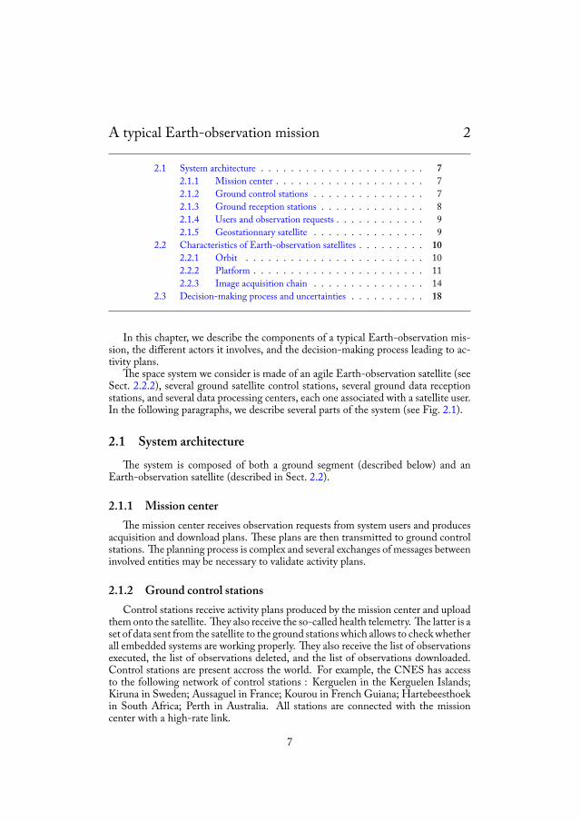
e space system we consider is made of an agile Earth-observation satellite (seeSect. 2.2.2), several ground satellite control stations, several ground data receptionstations, and several data processing centers, each one associated with a satellite user.In the following paragraphs, we describe several parts of the system (see Fig. 2.1).
2.1 System architecturee system is composed of both a ground segment (described below) and an
Earth-observation satellite (described in Sect. 2.2).
2.1.1 Mission centere mission center receives observation requests from system users and produces
acquisition and download plans. ese plans are then transmitted to ground controlstations. e planning process is complex and several exchanges of messages betweeninvolved entities may be necessary to validate activity plans.
2.1.2 Ground control stationsControl stations receive activity plans produced by the mission center and upload
them onto the satellite. ey also receive the so-called health telemetry. e latter is aset of data sent from the satellite to the ground stations which allows to check whetherall embedded systems are working properly. ey also receive the list of observationsexecuted, the list of observations deleted, and the list of observations downloaded.Control stations are present accross the world. For example, the CNES has accessto the following network of control stations : Kerguelen in the Kerguelen Islands;Kiruna in Sweden; Aussaguel in France; Kourou in French Guiana; Hartebeesthoekin South Africa; Perth in Australia. All stations are connected with the missioncenter with a high-rate link.
7
. A E -
F . : System architecture.
2.1.3 Ground reception stationsGround reception stations are exclusively used for receiving mission telemetry
which corresponds to data collected by the satellite instruments (images in an Earth-observation mission). Such data can be received when the satellite is in visibility, thatis when its telemetry antenna is able to communicate with the station antenna. Eachuser has one or several allowed stations for downloading data. Acquisitions receivedin a ground reception station are then sent to the user’s production center. e list ofacquisitions downloaded and the list of acquisitions stored on board the satellite aresent to the mission center. It is important to maintain consistency between groundstations and the satellite so that algorithms producing plans can rely on the mostrecent information. Because it is not always possible to maintain such a consistency,because of data transfer latency for example, it is also necessary to think about planrepair at execution when the plan built on the ground is not fully consistent with thereal state of the satellite.
8
2.1. System architecture
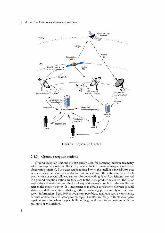
2.1.4 Users and observation requestsObservation requests are emitted by users of the system. Each observation is
de ned by:– a geographical zone to observe which is a polygon split into strips (see Fig.2.2);
each strip is referenced by its geographical coordinates, an observation dura-tion, a data volume; and sometimes weather forecast; the observation must becarried out during one of the visibility window of the strip;
– a priority level; priorities are said to be tight because the satisfaction of anyrequest of the high-priority is always preferred to the satisfaction of any set ofrequests of lower priorities;
– a weight, allowing to sort acquisitions which have the same priority level;– maximum observation angles: the larger the observation angle, the worst the
quality; the best quality is given with a nadir pointing , that is when the satelliteis pointing towards the center of the Earth.
polygon
strip
possible
acquired
directions
swath
F . : A geographical zone split into strips.
Once observation requests have been performed, associated data are sent to pro-duction centers which transform this raw mission telemetry into an image product.Each user of the system has its preferred production center.
2.1.5 Geostationnary satellitee network of ground reception stations for low Earth orbit satellites is not large
enough to cover the surface of the Earth. Geostationary satellites have a high altitudeof around 36000 kilometers which gives them a large coverage (1/3 of the Earth sur-face). anks to their orbit, their pointing is stationary above a given point. When alow-orbit satellite is ying over a zone without much ground reception stations, theonly way of immediately downloading data to the ground is to transmit data to geo-stationary satellites with an optical or a radio link. e geostationary satellite, withits much larger covering, will be able to download this data onto a ground receptionstation. is kind of satellite is frequently used in telecommunications and meteo-rology. In some missions, it is possible to make use of a network of geostationary
9
. A E -
satellites as a relay for downloading data to ground reception stations (such as theEuropean Data Relay System).
2.2 Characteristics of Earth-observation satellitesIn the following, we review some of the characteristics of a typical Earth-
observation satellite. We speak of attitude to designate the orientation of the satellitewith respect to an inertial frame of reference or another entity such as a planet. Asatellite is able to :
– perform attitude change maneuvers thanks to gyroscopic actuators. SeeSect. 2.2.2 for more details;
– perform orbital maneuvers thanks to engines with liquid propellants;– perform observations thanks to a telescope;– download observations thanks to a telemetry antenna;– perform heliocentric pointings, towards the sun, to ll up its batteries with
solar energy, and near-heliocentric pointings to favor download efficiency whilere lling the batteries;
– perform geocentric pointings towards the center of the Earth, to make com-munications with ground reception stations easier.
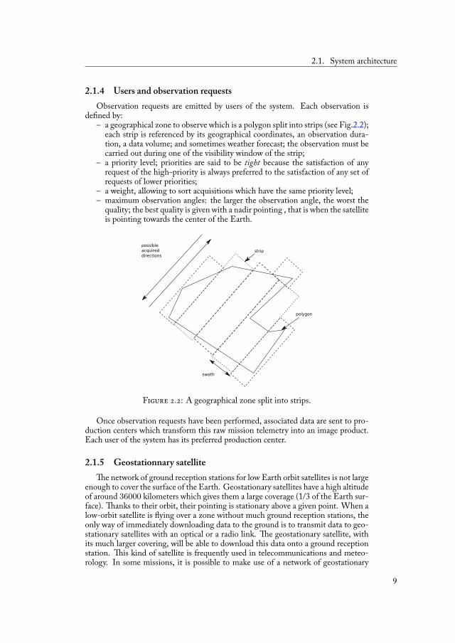
F . : View of an heliosynchronous orbit with respect to the Sun.
2.2.1 Orbite satellite is placed on a low geocentric orbit at an altitude between 700 and
1000 kilometers. is orbit is:– heliosynchronous: the angle between the orbit plan and the sun direction is
more or less constant (see Fig. 2.3) though the Earth equatorial bulges causesa precession on this orbit;
10

2.2. Characteristics of Earth-observation satellites
F . : Track of an heliosynchronous orbit.
– near-polar, the orbit is inclined compared to a line going from the North poleto the South pole but the inclination is very small, hence the satellite trajectoryis almost above the poles;
– of short periodicity; the satellite comes back frequently above a point at thesame solar hour (2 to 3 days).
Heliosynchronism combined to Earth rotation allows to cover almost entirelythe Earth surface in a given period (see Fig. 2.4). ese orbital characteristics favorsimilar sunshine conditions at each come back above a point which is interestingwhen one wishes to follow the evolution of a phenomena on the ground.
2.2.2 Platforme satellite considered in this manuscript must be compatible with the VEGA
European launcher, which is specialized in placing payload at low-orbit (see Fig. 2.5).e satellite mass will be less than 1500 kilograms, its power consumption will be
about 2 kilowatts, its lifetime will be 7 to 10 years, and it will be electrically or chem-ically propelled.
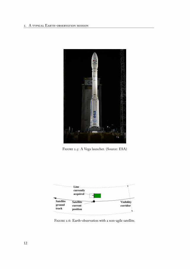
Agility Non-agile Earth-observing satellites have only one degree of freedomthanks to an orientable mirror put in front of each instrument. is mirror is ac-tionned on the roll axis between acquisitions. It allows the satellite to take image atthe right or left side of its ground track. An image is then produced by the movementof the satellite on its track on the ground (see Fig. 2.6). Time windows during whichimage acquisition is possible can be pre-computed for each observation request. In-deed, there is only one opportunity in each orbit to perform a given observation (seethe left of Fig. 2.7). When two opportunity windows overlap or are too close to eachother, it means that the two associated observations are not compatible. A choicehas then to be done. erefore, the resulting observation planning problem includesa selection problem.
In this study, we consider planning and scheduling for an agile Earth-observingsatellite (such as Pléiades). With this type of satellite, instruments and solar panelsare body-mounted (to avoid low-frequency attitude perturbations) and the platformis able to move quickly around its gravity center, along the roll, pitch and yaw axes,
11
. A E -
F . : A Vega launcher. (Source: ESA)
F . : Earth-observation with a non-agile satellite.
12

2.2. Characteristics of Earth-observation satellites
thanks to gyroscopic actuators, while moving along its orbit [Chrétien et al., 2004].e two additional agility axis, compared to the non-agile case, allow to greatly in-
crease the number of opportunities for image acquisitions. Indeed, the satellite canpoint ahead of its position or backwards with regard to nadir (see Fig. 2.8), the choiceof the start of acquisition becomes free in a time window that can be pre-computed(see Fig. 2.7). Such time windows are longer than when the satellite is not agile, andsome acquisitions that were not compatible become compatible thanks to this agility(see the right of Fig. 2.7). e resulting planning problem includes a selection and ascheduling problem, and it becomes more difficult.
corridorVisibility
Observationwindow
Satellitegroundtrack
observation
observation
corridorVisibility
Observationwindow
Visibilitywindow
Candidate
SelectedSatellitegroundtrack
F . : Comparison of observation capabilities between a non-agile satellite(left) and an agile satellite (right).
Moreover, for agile satellites, minimum transition durations between two suc-cessive observations depend on the start date of the transition (see Fig. 2.8). Com-puting these minimum durations is a continuous optimization problem under con-straints [Beaumet et al., 2007], which can be solved using solvers such as Real-Paver [Granvilliers and Benhamou, 2006] or IBEX [Chabert and Jaulin, 2009], orapproximate solution techniques (see Sect. 4.2.3).
e ability of the satellite to do attitude movements combined to its orbital tra-jectory allows to perform acquisitions by scanning the zone to acquire. Observationpro les, that is attitude movements done by the satellite while performing an obser-vation, are difficult to compute, and they depend on the start date of the observation.
13

. A E -
S2 S2 S2 S2
ground
satellite
Acq1 Acq2 Acq1 Acq2
F . : e duration of transition between two acquisitions depends on theangle to travel and then on the start date of the transition.
Orbital maneuver An orbital maneuver allows to change the orbit of a spacecraftthanks to a propeller system. For instance, orbital maneuvers are necessary to placespace probes into orbit around planets. Regularly, Earth-observation satellites de-viate from their orbit. It is then required to perform orbital maneuvers to rectifytheir trajectories. ese maneuvers, which are consuming propellant, are done abovezones that are not frequently observed such as poles.
2.2.3 Image acquisition chainWe now describe the onboard image acquisition chain that is visible on Fig. 2.9.
encryption
download
channels
instrument memory
memorybanks
datacompressors
detectorlines data
antennamobile
F . : How data is acquired, recorded, and downloaded.
2.2.3.1 TelescopeTo realize observations, the satellite is equipped with a telescope. Its large primary
mirror has a resolution of 20 to 30 centimeters and a swath of 15 to 20 kilometers.It is possible to take a minimum of 250 images per day. e focal plane is madeof several detector lines, each of which is dedicated to a frequency range. Severaldetector lines make an image channel. e following constraints must be taken intoaccount :
– a minimum pre-heating time is required before using the telescope;– the temperature increases linearly when the instrument is activated and has an
exponential decrease when the instrument is put off;– the temperature of the focal plane must not exceed a value which limits the
continuous period of use;– there must be a limited amount of ON/OFF cycles because they degrade the
instrument reliability;
14
2.2. Characteristics of Earth-observation satellites
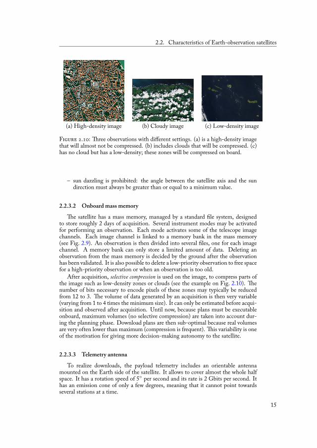
(a) High-density image (b) Cloudy image (c) Low-density image
F . : ree observations with different settings. (a) is a high-density imagethat will almost not be compressed. (b) includes clouds that will be compressed. (c)has no cloud but has a low-density; these zones will be compressed on board.
– sun dazzling is prohibited: the angle between the satellite axis and the sundirection must always be greater than or equal to a minimum value.
2.2.3.2 Onboard mass memory
e satellite has a mass memory, managed by a standard le system, designedto store roughly 2 days of acquisition. Several instrument modes may be activatedfor performing an observation. Each mode activates some of the telescope imagechannels. Each image channel is linked to a memory bank in the mass memory(see Fig. 2.9). An observation is then divided into several les, one for each imagechannel. A memory bank can only store a limited amount of data. Deleting anobservation from the mass memory is decided by the ground after the observationhas been validated. It is also possible to delete a low-priority observation to free spacefor a high-priority observation or when an observation is too old.
After acquisition, selective compression is used on the image, to compress parts ofthe image such as low-density zones or clouds (see the example on Fig. 2.10). enumber of bits necessary to encode pixels of these zones may typically be reducedfrom 12 to 3. e volume of data generated by an acquisition is then very variable(varying from 1 to 4 times the minimum size). It can only be estimated before acqui-sition and observed after acquisition. Until now, because plans must be executableonboard, maximum volumes (no selective compression) are taken into account dur-ing the planning phase. Download plans are then sub-optimal because real volumesare very often lower than maximum (compression is frequent). is variability is oneof the motivation for giving more decision-making autonomy to the satellite.
2.2.3.3 Telemetry antenna
To realize downloads, the payload telemetry includes an orientable antennamounted on the Earth side of the satellite. It allows to cover almost the whole halfspace. It has a rotation speed of 5 per second and its rate is 2 Gbits per second. Ithas an emission cone of only a few degrees, meaning that it cannot point towardsseveral stations at a time.
15
. A E -
Once the antenna pointing direction has been decided, the satellite-station track-ing is automatically carried on, taking into account current attitude movements. eground reception station and the satellite use ephemerides to track themselves mu-tually. It is also possible to have dynamical tracking by signal servoing between thesatellite and the station.
When planning downloads, one must take into account the rotation speed of theantenna, the satellite’s attitude and the station coordinates. A minimal transitionduration (that we will also call antenna transition) is required before starting commu-nication with a ground station even if the satellite is in the reception visibility coneof the station (pull-in time).
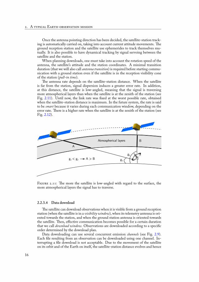
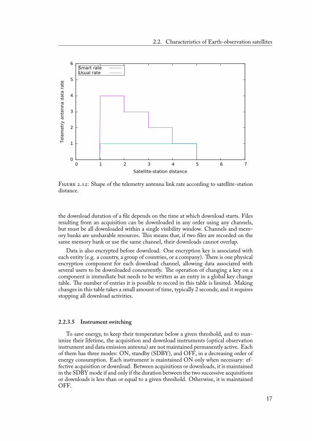
e antenna rate depends on the satellite-station distance. When the satelliteis far from the station, signal dispersion induces a greater error rate. In addition,at this distance, the satellite is low-angled, meaning that the signal is traversingmore atmospherical layers than when the satellite is at the zenith of the station (seeFig. 2.11). Until now, the link rate was xed at the worst possible rate, obtainedwhen the satellite-station distance is maximum. In the future system, the rate is saidto be smart because it varies during each communication window, depending on theerror rate. ere is a higher rate when the satellite is at the zenith of the station (seeFig. 2.12).
F . : e more the satellite is low-angled with regard to the surface, themore atmospherical layers the signal has to traverse.
2.2.3.4 Data downloade satellite can download observations when it is visible from a ground reception
station (when the satellite is in a visibility window), when its telemetry antenna is ori-ented towards the station, and when the ground station antenna is oriented towardsthe satellite. en, effective communication becomes possible for a certain durationthat we call download window. Observations are downloaded according to a speci corder determined by the download plan.
Data downloading can use several concurrent emission channels (see Fig. 2.9).Each le resulting from an observation can be downloaded using one channel. In-terrupting a le download is not acceptable. Due to the movement of the satelliteon its orbit and of the Earth on itself, the satellite-station distance evolves and hence
16
2.2. Characteristics of Earth-observation satellites
0
1
2
3
4
5
6
0 1 2 3 4 5 6 7
Tele
met
ry a
nten
na d
ata
rate
Satellite-station distance
Smart rateUsual rate
F . : Shape of the telemetry antenna link rate according to satellite-stationdistance.
the download duration of a le depends on the time at which download starts. Filesresulting from an acquisition can be downloaded in any order using any channels,but must be all downloaded within a single visibility window. Channels and mem-ory banks are unsharable resources. is means that, if two les are recorded on thesame memory bank or use the same channel, their downloads cannot overlap.
Data is also encrypted before download. One encryption key is associated witheach entity (e.g. a country, a group of countries, or a company). ere is one physicalencryption component for each download channel, allowing data associated withseveral users to be downloaded concurrently. e operation of changing a key on acomponent is immediate but needs to be written as an entry in a global key changetable. e number of entries it is possible to record in this table is limited. Makingchanges in this table takes a small amount of time, typically 2 seconds; and it requiresstopping all download activities.
2.2.3.5 Instrument switching
To save energy, to keep their temperature below a given threshold, and to max-imize their lifetime, the acquisition and download instruments (optical observationinstrument and data emission antenna) are not maintained permanently active. Eachof them has three modes: ON, standby (SDBY), and OFF, in a decreasing order ofenergy consumption. Each instrument is maintained ON only when necessary: ef-fective acquisition or download. Between acquisitions or downloads, it is maintainedin the SDBY mode if and only if the duration between the two successive acquisitionsor downloads is less than or equal to a given threshold. Otherwise, it is maintainedOFF.
17

. A E -
2.2.3.6 Instrument temperatureIf we consider an acquisition and download schedule, including the associated
instrument switching plan, we can build an approximation of the temperature pro leof each instrument and check whether or not temperature is always lower than orequal to a maximum acceptable level. Important margins are used in that domainbecause it is very difficult to model thermal interactions between the platform andthe instruments.
2.2.3.7 Onboard energyEnergy is consumed by the satellite platform, and by the acquisition and download
instruments according to their current mode (ON, SDBY, or OFF). It is producedby solar panels which are body-mounted on the satellite. Because the satellite orbitis quasi-polar, low-altitude, and helio-synchronous, it alternates day and night pe-riods (eclipse of the Sun by the Earth during night periods). Energy production isonly possible during day periods and, within these periods, it depends on the satelliteattitude trajectory. Produced energy is stored in batteries whose capacity is limited.See Fig. 2.13 for a typical energy pro le. Emax is the maximum energy level, equalto the battery capacity: the energy level cannot be greater than Emax. Emin is theminimum acceptable energy level: the energy level must not be lower than Emin. Ifwe consider an acquisition and download schedule, including the associated instru-ment switching plan, we can build the associated energy pro le and check whetheror not the energy level is always greater than or equal to Emin.
time
levelenergy
Emax
Emin
0
F . : Typical energy pro le.
2.3 Decision-making process and uncertaintiese satellite evolves in a dynamic environment and it must face several sources of
uncertainty :– the cloud coverage, conditioning the success of observations; weather forecasts
are useful but not always accurate;– the volume of les after selective compression; because the cloud coverage is
not exactly known in advance, the compression rate is not known either;– the reliability of the onboard/ground data link, which is in uenced by interfer-
ences; the actual quality of the data link can alter download durations;– the energy available on board, hard to model because it varies according to the
production by the solar panels and the consumption by the satellite systems;
18

2.3. Decision-making process and uncertainties
F . : Timelines representing a plan execution.
– the arrival of new urgent observation requests.ese uncertainties in uence activity planning. We say that the environment and
the resulting planning problem are dynamic because problem parameters are quicklyevolving. Planning and scheduling problems with uncertainties results in large searchspaces (as it includes hundreds of acquisitions per day in our case). Plans not takingthese uncertainties into account are destined to fail [Bresina et al., 2002b]. e cur-rent approach consists in building plans offline on the ground (typically every 8 hourswith a 24-hour gliding planning horizon), where acquisition and download schedulesare produced with precise start and end times for activities. ese schedules verifyall the constraints related to satellite attitude, to acquisition and download, and toonboard energy, memory, and temperature. ey are uploaded to the satellite duringground control station visibility windows and executed by the satellite without anychange (see typical timelines on Fig. 2.14).
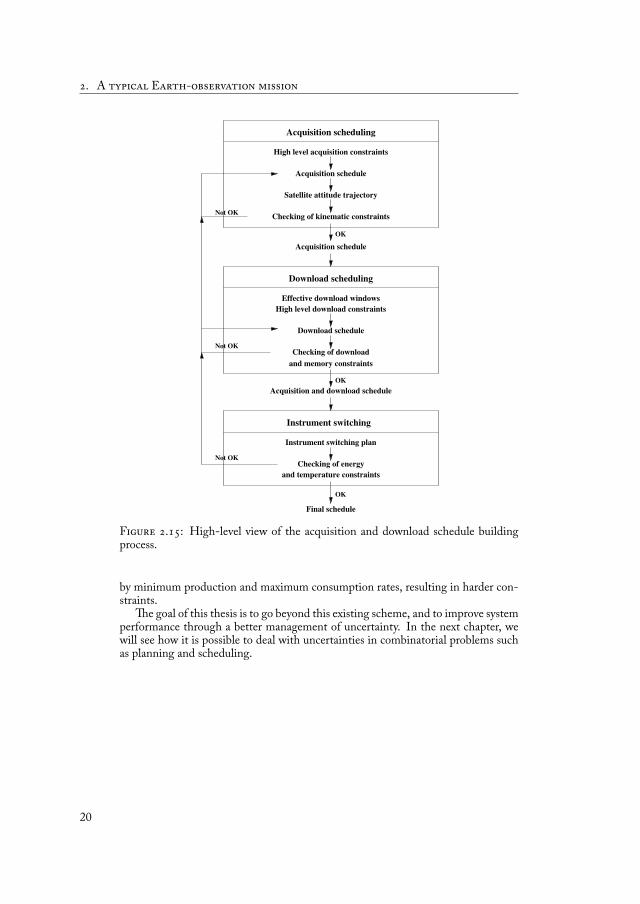
e existing acquisition and download schedule building process is illustrated inFig. 2.15. At the highest level, an acquisition schedule and then a download scheduleare proposed, taking into account user request priorities and high-level aggregatedconstraints such as no more acquisition time than a given threshold over each satelliterevolution or each set of consecutive satellite revolutions. e proposed schedules arethen checked according to all the constraints. In case of any constraint violation, theyare modi ed by removing for example some acquisitions or downloads. e processcontinues until a schedule that satis es all the constraints is found. is processalways terminates because an empty schedule (no acquisition and no download) isalways feasible if we assume a nominal satellite state and behavior.
To be sure that the proposed schedule is really executable by the satellite in spiteof the numerous uncertainties, safety margins are used when checking constraints.For example, the expected energy production and consumption rates are replaced
19
. A E -
F . : High-level view of the acquisition and download schedule buildingprocess.
by minimum production and maximum consumption rates, resulting in harder con-straints.
e goal of this thesis is to go beyond this existing scheme, and to improve systemperformance through a better management of uncertainty. In the next chapter, wewill see how it is possible to deal with uncertainties in combinatorial problems suchas planning and scheduling.
20
Combinatorial optimization under uncertainty 3
3.1 General considerations . . . . . . . . . . . . . . . . . . . . 213.2 Planning under uncertainty . . . . . . . . . . . . . . . . . . 25
3.2.1 Conformant planning . . . . . . . . . . . . . . . . 253.2.2 Contingent planning . . . . . . . . . . . . . . . . 263.2.3 Markov Decision Processes . . . . . . . . . . . . . 273.2.4 Hindsight optimization . . . . . . . . . . . . . . . 293.2.5 Monte Carlo Tree Search . . . . . . . . . . . . . . 29
3.3 Managing time and resources under uncertainty . . . . . . . 323.3.1 Job-Shop scheduling . . . . . . . . . . . . . . . . 323.3.2 Resource-Constrained Project Scheduling Problem . 323.3.3 Simple Temporal Networks . . . . . . . . . . . . . 34
3.4 Combinatorial optimization under uncertainty . . . . . . . . 363.4.1 Uncertainty in constraint programming . . . . . . . 363.4.2 Online stochastic combinatorial optimization . . . . 37
3.5 Planning and scheduling in the space domain . . . . . . . . . 39
“Une fois pris dans l ’événement, les hommes ne s’eneffraient plus. Seul l ’inconnu épouvante les hommes.”
— Antoine de Saint-Exupéry, Terre des hommes
Combinatorial optimization is a branch of mathematical optimization. e goal,in a combinatorial optimization problem, is to nd the best element in a nite setof possible elements. Generally, this set is very large and complete exploration isimpossible. Some methods have been developed to solve speci c problems such asplanning or scheduling. In this chapter, we brie y review techniques developed fortackling these problems in uncertain environments.
3.1 General considerationsFirst, we de ne some useful notions.
Determinism Determinism is a simpli cation of the world where actions have onlyone possible known outcome. In a deterministic world, results of successive dicerollings are known because all factors having an impact are known as well as theevolution of these factors.
Non-determinism is more realistic and proposes to model all the possible out-comes of an action. For example, an action can either succeed or fail. Taking this into
21

. C
account may be of importance for critical systems. Planning in non-deterministic do-mains features several difficulties compared to deterministic planning. On one hand,problem modeling is harder in terms of granularity and comprehensiveness becauseadditional variables have to be added to represent uncertainty. On the other hand,the search space is much larger and then longer to explore. When the different out-comes of an action can be associated with a probability, we speak of a stochastic action(see Fig. 3.1).
F . : Difference between a deterministic action, a non-deterministic action,and a stochastic action. e action in the upper-left part is deterministic, it hasonly one outcome. e action in the upper-right part is non-deterministic, it hasseveral outcomes. e action in the bottom part is stochastic, it has several outcomes,weighted by a probability of occurrence.
Observability Once sources of uncertainty have been sorted out, it is possible tocharacterize them. e state of the system is considered to be the set of variablesneeded to make a decision involving the system. For example, it may be the positionof a robot or the available power in its batteries. A state is said to be totally observableif the agent knows the values of all variables at every time. It is partially observablewhen the value of some of the variables is not accessible. In this case, the planningsystem may have to make assumptions about these variables.
Robust planning and scheduling Several de nitions are possible for robust plan-ning and scheduling but it is an important subject with regard to uncertainty. Arobust plan can be a plan that maximizes an expected reward but it can also be a planbuilt offline with the aim of resisting or absorbing the exogenous events that could dis-turb the execution [Cichy et al., 2005] (meaning that uncertain parameters revealedduring the online phase should not impact the plan built during the offline phase),a plan ensuring that the solution quality will not deteriorate [Sevaux and Sörensen,2002], or a plan which can be quickly adapted in face of the events encountered atexecution [Ginsberg et al., 1998].
Globally, the principle of robust planning and scheduling is to minimize the num-ber of changes at execution but it is not practicable to consider only an offline phaseunless the environment is assumed to be deterministic [Rasconi et al., 2010]. Someauthors are proposing methods to evaluate the robustness of such robust plans [Fox
22

3.1. General considerations
et al., 2006b] [Rasconi et al., 2010]. For example, in our case, a satellite activity planis built to satisfy several users. e level of satisfaction is measurable for each user.One of the goal can be to stabilize this level of satisfaction when replanning com-pared to a previous plan. ese levels of satisfaction depend on agreements betweenusers before sending the plan on board. If the system is supposed to be reliable, itshould automatically take these levels into account when planning.
Phases of decision-making In deterministic decision-making, available actions aredeterministic. When planning, data is supposed to be available and a plan can becomputed. It is often easier to compute a plan of good quality in this setting althoughit may be inconsistent with the environment when it is executed. In decision-makingunder uncertainty, data is not supposed to be complete when planning and/or it isupdated during execution. We then distinguish two phases in decision-making:
– the offline phase which is the phase before the execution of the plan; duringthis phase, only a part of the data is known;
– the online phase which is the phase during the execution of the plan; duringthis phase, uncertainties are progressively cleared up.
For example, if we look at a scheduling problem, we can de ne two subproblems: the static subproblem and the dynamic subproblem [Rasconi et al., 2010]. estatic subproblem (offline phase) consists in assigning start dates and end dates toactivities while ensuring constraints and optimizing a criterion. e dynamic sub-problem (online phase) consists in monitoring the execution and in repairing the planwhen necessary. In our satellite case, we have three phases : offline phases on theground, offline phases on board and online phases on board (see Sect. 6.1). We willsee that the planning and scheduling frameworks presented in this chapter can alsobe distributed among three categories: proactive approaches, reactive approaches, andexible approaches. Each category address more or less a speci c decicion-making
phase.
Proactive approaches A way of dealing with problems that include uncertainty isto adopt a proactive approach, that is to take uncertainty into account mainly duringthe offline phase. It can be done by modeling the missing or uncertain informationand by building a plan or a family of plans which will be the most efficient in thelight of the information that is available when planning. In this setting, we considerthat it is possible to anticipate uncertain events and that the resulting plan will onlyneed minor changes at execution. Most of the approaches presented from Sect. 3.2can be used as proactive planning schemes.
Reactive approaches Another way of planning in a dynamic and uncertain contextis to build a plan during the online phase, that is when most uncertainties have beencleared up. is approach often needs a fast decision-making paired with an imme-diate execution. Decisions may be locally optimal but are seldom globally optimal.Local repair is a reactive approach that is applied when a baseline plan becomes in-consistent because of exogenous events. e objective is to make the plan consistentagain by making a relatively small number of changes. Compared to replanning, lo-cal repair does not start from scratch. It can be an interesting approach when planstability is wanted, that is when the number of changes has to be minimized.
When a baseline plan is computed in the offline phase, reactive approachescan be local [Smith, 1995] if a relatively small set of activities is updated, or
23

. C
global if the whole plan becomes inconsistent [Sakkout and Wallace, 2000]. Re-active planning approaches have been experimentally used in the space domainwith CASPER [Knight et al., 2001] [Chien et al., 2004b] on the EO-1 satellite,RAX [Bernard et al., 1998], PROBA [Teston et al., 1999] and RASSO [de No-vaes Kucinskis et al., 2007] to deal with real-time events such as natural phe-nomenons. In [Beaumet et al., 2011], authors have investigated a reactive onboardplanning scheme for an agile Earth-observing satellite. In [Fox et al., 2006a], re-planning and local repair are compared and it is shown that the latter allows a greaterplan stability. Plan repair is also used in IxTeT-Exec, an extension of the temporalplanner IxTeT which is dedicated to plan execution [Lemai and Ingrand, 2004]. InIxTeT-Exec, replanning is used when it is impossible to repair the current plan. InASPEN, which is used in space missions, an iterative con ict repair is continuallyupdating the plan according to the events [Rabideau et al., 1999]. More generally,these approaches are exploring the links between planning and execution in criticalenvironments. Several methods may be considered for handling uncertainty aboutthe future in a reactive planning framework:
– the future is determinized, meaning that one outcome is chosen for each actionamong the set of possible outcomes;
– the future is stochastic and sampling is performed to make the problemtractable; we will see several methods such as Hindsight Optimization, Monte-Carlo based methods, and Online Stochastic Combinatorial Optimization whichcan be used in a reactive framework.
Flexible approaches Flexible planning and scheduling is a combination of proac-tive and reactive approaches. Over the whole set of decisions to be made, some aremade offline and some are made online or closer to execution. is allows to dividethe workload between the two phases. Computing resources are often more impor-tant during the offline phase but uncertainties are large. On the contrary, during theonline phase, computing resources and uncertainties are low. Flexible approachesproduce plans which are designed to be adapted during the online phase. Note thatthough we present these methods as exible, it is true that boundaries between ex-ible, reactive, and proactive approaches are sometimes a bit fuzzy.
In scheduling, there exist several forms of exibility : temporal exibility, exi-bility on resource access order and exibility on resource assignment [Billaut et al.,2013]. In [Wu et al., 1999], partial-order plans are built, providing temporal exibil-ity. Highly constrained subsets of activities are partially ordered. Temporal aspectssuch as exact start dates are set only at execution. is approach requires high com-puting resources both when planning and when executing to transform the offlineorder into a executable plan. Partial-Order Schedules (POS) synthesis [Policella et al.,2004b] also provides temporal exibility. A POS is a graph where nodes representactivities and edges represent precedence constraints between pairs of activities suchthat any temporal solution (start and end dates) enforcing these constraints betweenactivities is valid. e approach follows a least commitment strategy in which tasksare ordered according to their needs in resources. For that, precedence constraintsare introduced for tasks accessing the same resource. Almost no computation is re-quired online because all con icts have been solved contrarily to the previous ap-proach. In [Policella et al., 2009], robust and exible plans are built from completelyinstantiated plans. To do that, a high-quality plan is rst built. en, temporalexibility is added by transforming the plan structure into a Partial Order Schedule.
In this method, the transformation of an instantiated plan into a exible plan does
24
3.2. Planning under uncertainty
not diminish the plan quality in terms of criterion. On the other hand, a very high-quality plan can be difficult to transform because it is highly constrained and adjusted.In [Orlandini et al., 2011], temporally exible plans are represented as automatons(Timed Game Automaton) which makes them veri able (using a reachability game)with a formal veri cation tool (UPPAAL-TIGA [Behrmann et al., 2007]). In theparametric dispatching approach [Gerber et al., 1995], the goal is to schedule tasksin a real time system. ese tasks are ordered in a list and have temporal constraints.In this approach, there are two components : an offline component that computeslower and upper parametric bounds for each task such that each bound is a functionof the actual realization date of the predecessors of the task. Only the rst task hasnon-parametric bounds. Parametric bounds allow to have exibility when executingthe schedule. e online component updates these bounds and launches the tasks:when the actual bounds of a task are computed, the online component may dispatchthe task during the time window de ned by the bounds. Another form of exibilityconsists in optimizing not only several temporal or resource instantiations given aunique baseline plan but how plans can be quickly changed at execution. For ex-ample, in [Jensen, 2003], the objective is to build a plan that is easily adaptable onboard when unexpected events occur. For that, the optimization focuses not only ona speci c plan but on a neighborhood of plans. In case of replanning, a high-qualityplan is easily found in the immediate neighborhood.
3.2 Planning under uncertaintyWe now give a closer look to a classical combinatorial optimization problem,
planning, as it has many common features with our data download and observationproblems. A classical planning model Q is de ned as a tuple Q = ⟨S, s0, SG, A, f⟩where:
– S is a nite set of states;– s0 ∈ S is the initial state,– SG ⊆ S is the set of goal states,– A is the set of operators (the actions),– a state transition function f : S ×A→ S : (s, a)→ f(s, a) = s′.More precisely, given a description of the initial state of the world, a description
of the desired goals, and a description of a set of possible actions, the solution to aplanning problem is a plan, that is a sequence of actions, that leads to one of the goalstates. Several strategies exist for problem involving uncertainty about the effects, thatis the result of the state transition function, or durations of actions.
3.2.1 Conformant planningOne of the most important assumption when planning concerns state observability
and several planning frameworks are developed to address each possible assumption.Conformant planning is a sub eld of classical planning where the aim is to nda plan, in a non-deterministic domain, guaranteeing that the goal will be reachedwith no observability, that is when the result of actions is not known at execution.In a classical planning problem, there is an initial state, a goal and a set of actionsthat modify the state. A solution to such a problem is a sequence of actions thatleads from the initial state to the goal. In conformant planning, the goal must bereached whatever the effects of the actions and whatever the initial state among aset of possible initial states [Hoffmann and Brafman, 2006]. is problem is then
25

. C
much more complex than classical planning. Verifying a conformant plan is a hardproblem in itself because one has to explore all the possible outcomes of the actions.To solve this problem, it is possible to search in the space of belief states, that is thespace where the elements are the possible states of the world given actions previouslyexecuted. Unfortunately, the number of elements in this space is exponential withregards to the state space. Authors are then trying to represent these elements in themost compact way and in developing efficient heuristics to quickly move into thisspace [Palacios and Geffner, 2009]. See Fig. 3.2 for an illustration of the space ofbelief states and an example of conformant plan.
Start
a2
action effects
Start
(a) Belief space after action a1 (b) Belief space after action a2
Start
(c) Belief space after
sequence (a2, a2)
Conformant plan
a1
F . : A conformant plan for a robot moving on a grid. Action a1 is deter-ministic, action a2 is non-deterministic. Whatever the initial position of the roboton the grid and the action effects, the execution of the conformant plan will succeedin reaching the goal. Belief spaces in different cases is also shown.
Although the idea of computing a plan or a schedule that will always remainconsistent is interesting, modeling our problems as conformant planning problemswould not be satisfactory. Indeed, our problems do not need the assumption of noobservability to be solved as uncertain parameters are observable on board the satel-lite. In addition, building a conformant plan for the data download problem wouldconsists in assuming maximum volumes for all observations as it is already the casein the current approach and is too pessimistic.
3.2.2 Contingent planningConformant planning is adapted when the environment is not observable at all.
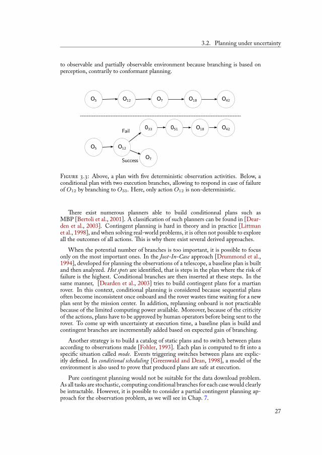
When observations are available, other frameworks are used. Recall that when theactions are non-deterministic, several outcomes are possible for each action. Withconditional planning, the plan is adapted to observed outcomes of actions and to ob-served exogenous events. A conditional plan has several execution branches dependingon the current state of the system. e plan produced is not a sequence of actionsbut a directed root tree or a directed acyclic graph where each path from the root toa leaf is a complex execution sequence (see Fig. 3.3). is type of plan is tailored
26
3.2. Planning under uncertainty
to observable and partially observable environment because branching is based onperception, contrarily to conformant planning.
F . : Above, a plan with ve deterministic observation activities. Below, aconditional plan with two execution branches, allowing to respond in case of failureof O12 by branching to O33. Here, only action O12 is non-deterministic.
ere exist numerous planners able to build conditionnal plans such asMBP [Bertoli et al., 2001]. A classi cation of such planners can be found in [Dear-den et al., 2003]. Contingent planning is hard in theory and in practice [Littmanet al., 1998], and when solving real-world problems, it is often not possible to exploreall the outcomes of all actions. is is why there exist several derived approaches.
When the potential number of branches is too important, it is possible to focusonly on the most important ones. In the Just-In-Case approach [Drummond et al.,1994], developed for planning the observations of a telescope, a baseline plan is builtand then analyzed. Hot spots are identi ed, that is steps in the plan where the risk offailure is the highest. Conditional branches are then inserted at these steps. In thesame manner, [Dearden et al., 2003] tries to build contingent plans for a martianrover. In this context, conditional planning is considered because sequential plansoften become inconsistent once onboard and the rover wastes time waiting for a newplan sent by the mission center. In addition, replanning onboard is not practicablebecause of the limited computing power available. Moreover, because of the criticityof the actions, plans have to be approved by human operators before being sent to therover. To come up with uncertainty at execution time, a baseline plan is build andcontingent branches are incrementally added based on expected gain of branching.
Another strategy is to build a catalog of static plans and to switch between plansaccording to observations made [Fohler, 1993]. Each plan is computed to t into aspeci c situation called mode. Events triggering switches between plans are explic-itly de ned. In conditional scheduling [Greenwald and Dean, 1998], a model of theenvironment is also used to prove that produced plans are safe at execution.
Pure contingent planning would not be suitable for the data download problem.As all tasks are stochastic, computing conditional branches for each case would clearlybe intractable. However, it is possible to consider a partial contingent planning ap-proach for the observation problem, as we will see in Chap. 7.
27
. C
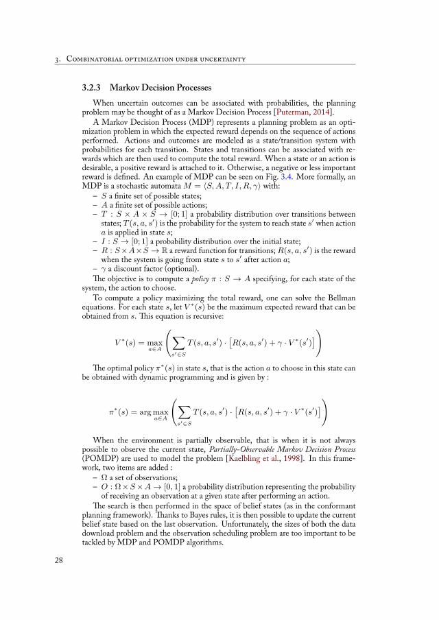
3.2.3 Markov Decision ProcessesWhen uncertain outcomes can be associated with probabilities, the planning
problem may be thought of as a Markov Decision Process [Puterman, 2014].A Markov Decision Process (MDP) represents a planning problem as an opti-
mization problem in which the expected reward depends on the sequence of actionsperformed. Actions and outcomes are modeled as a state/transition system withprobabilities for each transition. States and transitions can be associated with re-wards which are then used to compute the total reward. When a state or an action isdesirable, a positive reward is attached to it. Otherwise, a negative or less importantreward is de ned. An example of MDP can be seen on Fig. 3.4. More formally, anMDP is a stochastic automata M = ⟨S, A, T, I, R, γ⟩ with:
– S a nite set of possible states;– A a nite set of possible actions;– T : S × A × S → [0; 1] a probability distribution over transitions between
states; T (s, a, s′) is the probability for the system to reach state s′ when actiona is applied in state s;
– I : S → [0; 1] a probability distribution over the initial state;– R : S×A×S → R a reward function for transitions; R(s, a, s′) is the reward
when the system is going from state s to s′ after action a;– γ a discount factor (optional).
e objective is to compute a policy π : S → A specifying, for each state of thesystem, the action to choose.
To compute a policy maximizing the total reward, one can solve the Bellmanequations. For each state s, let V ∗(s) be the maximum expected reward that can beobtained from s. is equation is recursive:
V ∗(s) = maxa∈A
(∑s′∈S
T (s, a, s′) ·[R(s, a, s′) + γ · V ∗(s′)
])e optimal policy π∗(s) in state s, that is the action a to choose in this state can
be obtained with dynamic programming and is given by :
π∗(s) = arg maxa∈A
(∑s′∈S
T (s, a, s′) ·[R(s, a, s′) + γ · V ∗(s′)
])
When the environment is partially observable, that is when it is not alwayspossible to observe the current state, Partially-Observable Markov Decision Process(POMDP) are used to model the problem [Kaelbling et al., 1998]. In this frame-work, two items are added :
– Ω a set of observations;– O : Ω×S×A→ [0, 1] a probability distribution representing the probability
of receiving an observation at a given state after performing an action.e search is then performed in the space of belief states (as in the conformant
planning framework). anks to Bayes rules, it is then possible to update the currentbelief state based on the last observation. Unfortunately, the sizes of both the datadownload problem and the observation scheduling problem are too important to betackled by MDP and POMDP algorithms.
28
3.2. Planning under uncertainty
F . : Example of an MDP representing a planning problem involving a robotequipped with a sensor. Rectangles are states, actions are circles. e robot can movearound and try to acquire an image. A reward is obtained if the target is acquired.
ere are deterministic actions such as Move or Stop and stochastic actions. esensor error is modeled as a failure probability. Here the optimal policy is to get tostate not moving and then to try to acquire the target. e expected gain is thenmaximized.
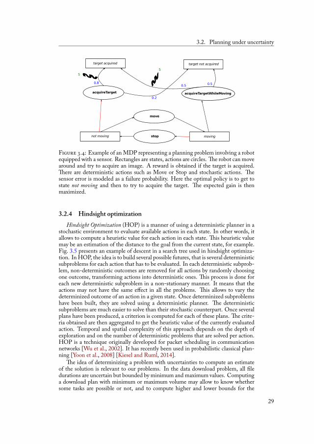
3.2.4 Hindsight optimizationHindsight Optimization (HOP) is a manner of using a deterministic planner in a
stochastic environment to evaluate available actions in each state. In other words, itallows to compute a heuristic value for each action in each state. is heuristic valuemay be an estimation of the distance to the goal from the current state, for example.Fig. 3.5 presents an example of descent in a search tree used in hindsight optimiza-tion. In HOP, the idea is to build several possible futures, that is several deterministicsubproblems for each action that has to be evaluated. In each deterministic subprob-lem, non-deterministic outcomes are removed for all actions by randomly choosingone outcome, transforming actions into deterministic ones. is process is done foreach new deterministic subproblem in a non-stationary manner. It means that theactions may not have the same effect in all the problems. is allows to vary thedeterminized outcome of an action in a given state. Once determinized subproblemshave been built, they are solved using a deterministic planner. e deterministicsubproblems are much easier to solve than their stochastic counterpart. Once severalplans have been produced, a criterion is computed for each of these plans. e crite-ria obtained are then aggregated to get the heuristic value of the currently evaluatedaction. Temporal and spatial complexity of this approach depends on the depth ofexploration and on the number of deterministic problems that are solved per action.HOP is a technique originally developed for packet scheduling in communicationnetworks [Wu et al., 2002]. It has recently been used in probabilistic classical plan-ning [Yoon et al., 2008] [Kiesel and Ruml, 2014].
e idea of determinizing a problem with uncertainties to compute an estimateof the solution is relevant to our problems. In the data download problem, all ledurations are uncertain but bounded by minimum and maximum values. Computinga download plan with minimum or maximum volume may allow to know whethersome tasks are possible or not, and to compute higher and lower bounds for the
29
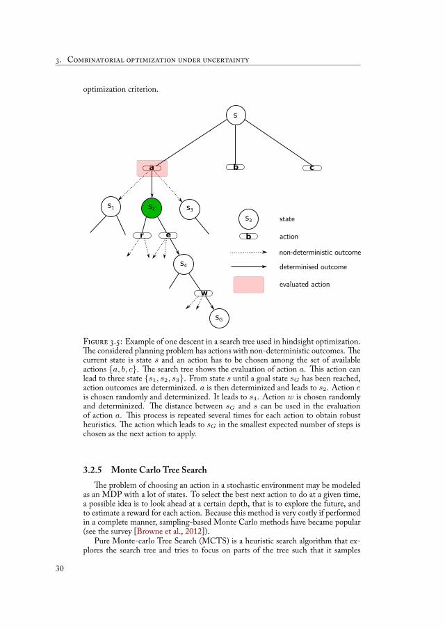
. C
optimization criterion.
F . : Example of one descent in a search tree used in hindsight optimization.e considered planning problem has actions with non-deterministic outcomes. e
current state is state s and an action has to be chosen among the set of availableactions a, b, c. e search tree shows the evaluation of action a. is action canlead to three state s1, s2, s3. From state s until a goal state sG has been reached,action outcomes are determinized. a is then determinized and leads to s2. Action eis chosen randomly and determinized. It leads to s4. Action w is chosen randomlyand determinized. e distance between sG and s can be used in the evaluationof action a. is process is repeated several times for each action to obtain robustheuristics. e action which leads to sG in the smallest expected number of steps ischosen as the next action to apply.
3.2.5 Monte Carlo Tree Searche problem of choosing an action in a stochastic environment may be modeled
as an MDP with a lot of states. To select the best next action to do at a given time,a possible idea is to look ahead at a certain depth, that is to explore the future, andto estimate a reward for each action. Because this method is very costly if performedin a complete manner, sampling-based Monte Carlo methods have became popular(see the survey [Browne et al., 2012]).
Pure Monte-carlo Tree Search (MCTS) is a heuristic search algorithm that ex-plores the search tree and tries to focus on parts of the tree such that it samples
30
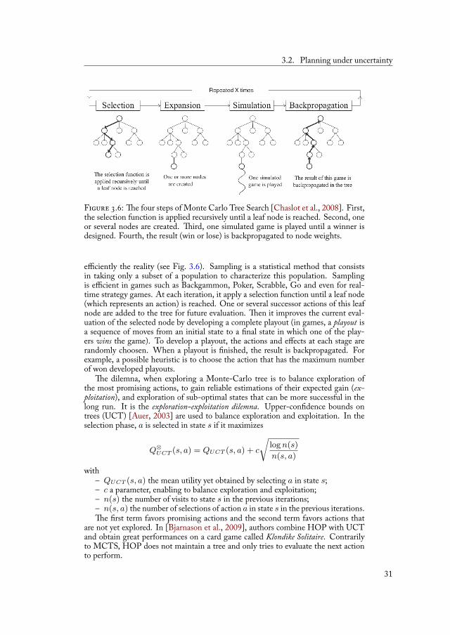
3.2. Planning under uncertainty
F . : e four steps of Monte Carlo Tree Search [Chaslot et al., 2008]. First,the selection function is applied recursively until a leaf node is reached. Second, oneor several nodes are created. ird, one simulated game is played until a winner isdesigned. Fourth, the result (win or lose) is backpropagated to node weights.
efficiently the reality (see Fig. 3.6). Sampling is a statistical method that consistsin taking only a subset of a population to characterize this population. Samplingis efficient in games such as Backgammon, Poker, Scrabble, Go and even for real-time strategy games. At each iteration, it apply a selection function until a leaf node(which represents an action) is reached. One or several successor actions of this leafnode are added to the tree for future evaluation. en it improves the current eval-uation of the selected node by developing a complete playout (in games, a playout isa sequence of moves from an initial state to a nal state in which one of the play-ers wins the game). To develop a playout, the actions and effects at each stage arerandomly choosen. When a playout is nished, the result is backpropagated. Forexample, a possible heuristic is to choose the action that has the maximum numberof won developed playouts.
e dilemna, when exploring a Monte-Carlo tree is to balance exploration ofthe most promising actions, to gain reliable estimations of their expected gain (ex-ploitation), and exploration of sub-optimal states that can be more successful in thelong run. It is the exploration-exploitation dilemna. Upper-con dence bounds ontrees (UCT) [Auer, 2003] are used to balance exploration and exploitation. In theselection phase, a is selected in state s if it maximizes
Q⊗UCT (s, a) = QUCT (s, a) + c
√log n(s)n(s, a)
with– QUCT (s, a) the mean utility yet obtained by selecting a in state s;– c a parameter, enabling to balance exploration and exploitation;– n(s) the number of visits to state s in the previous iterations;– n(s, a) the number of selections of action a in state s in the previous iterations.
e rst term favors promising actions and the second term favors actions thatare not yet explored. In [Bjarnason et al., 2009], authors combine HOP with UCTand obtain great performances on a card game called Klondike Solitaire. Contrarilyto MCTS, HOP does not maintain a tree and only tries to evaluate the next actionto perform.
31

. C
e idea of sampling may be interesting for our problems as their search spacesare very large. It would allow to reduce the number of search steps and still to takeuncertainty into account.
3.3 Managing time and resources under uncertaintyWe have seen that several techniques allow planning under uncertainty. Our
problems have planning features but also scheduling features. In this section, we ad-dress scheduling under uncertainty. e computational effort for solving schedulingproblems focuses on allocating time and resources to tasks. Managing uncertaintyin scheduling problems is very important in applications because, for example, taskssuch as manufacturing have rarely xed and known durations, and external eventsmay disturb the initial schedule. It is then necessary to have strategies to ensure thatexecution will not fail.
3.3.1 Job-Shop schedulingIn this section, we look at pure scheduling problems. Details on these problems
can be found in [Pinedo, 2012]. e Job-Shop Scheduling Problem ( JSSP) consistsin scheduling each job Ji in a set J = J1, ..., Jn onto M = M1, ..., Mmidentical machines while minimizing the total makespan, that is the total length ofthe schedule (see an example on Fig. 3.7). Each job is made of an ordered sequenceof tasks. Each task must be processed during an uninterrupted period on a machine.
e original problem is an online problem where jobs arrive one at a time and mustbe dispatched in an industrial manufacturing context. In the JSSP the route of jobis xed. It means that an order for tasks to be processed on machines is given asinput. is order is not given in the Open-Shop version of the problem. e FlexibleJob-Shop (FJSSP) version is even less restrictive as it allows a job to be processed byany machine of a given set. FJSSP is close to our data download problem whereles from observations are stored onto memory banks and have to be scheduled onto
identical communication channels. Finally, note that there exists a stochastic versionof the problem [Mahdavi et al., 2010] which can take into account machine failuresand stochastic task durations.
F . : Solution to a Job-Shop problem with 3 machines and 3 jobs.
3.3.2 Resource-Constrained Project Scheduling Probleme Resource-Constrained Project Scheduling Problem (RCPSP/max) [Bartusch
et al., 1988] is a classic NP-hard problem that has several real-world applications inlogistics and project scheduling. It is more general than the job-shop scheduling
32
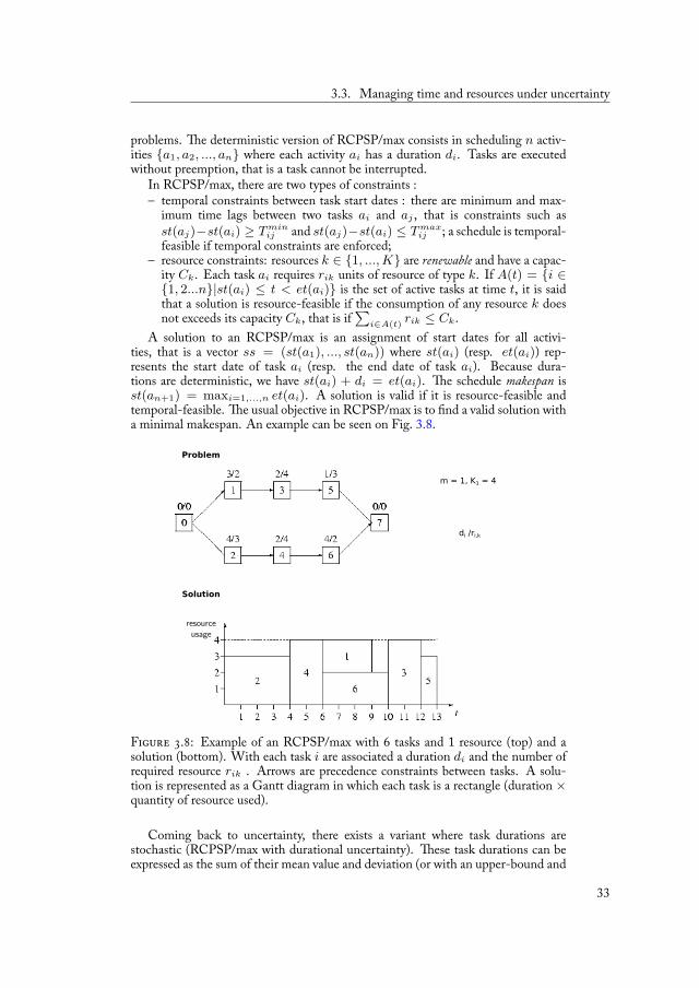
3.3. Managing time and resources under uncertainty
problems. e deterministic version of RCPSP/max consists in scheduling n activ-ities a1, a2, ..., an where each activity ai has a duration di. Tasks are executedwithout preemption, that is a task cannot be interrupted.
In RCPSP/max, there are two types of constraints :– temporal constraints between task start dates : there are minimum and max-
imum time lags between two tasks ai and aj , that is constraints such asst(aj)−st(ai) ≥ T min
ij and st(aj)−st(ai) ≤ T maxij ; a schedule is temporal-
feasible if temporal constraints are enforced;– resource constraints: resources k ∈ 1, ..., K are renewable and have a capac-
ity Ck. Each task ai requires rik units of resource of type k. If A(t) = i ∈1, 2...n|st(ai) ≤ t < et(ai) is the set of active tasks at time t, it is saidthat a solution is resource-feasible if the consumption of any resource k doesnot exceeds its capacity Ck, that is if
∑i∈A(t) rik ≤ Ck.
A solution to an RCPSP/max is an assignment of start dates for all activi-ties, that is a vector ss = (st(a1), ..., st(an)) where st(ai) (resp. et(ai)) rep-resents the start date of task ai (resp. the end date of task ai). Because dura-tions are deterministic, we have st(ai) + di = et(ai). e schedule makespan isst(an+1) = maxi=1,...,n et(ai). A solution is valid if it is resource-feasible andtemporal-feasible. e usual objective in RCPSP/max is to nd a valid solution witha minimal makespan. An example can be seen on Fig. 3.8.
F . : Example of an RCPSP/max with 6 tasks and 1 resource (top) and asolution (bottom). With each task i are associated a duration di and the number ofrequired resource rik . Arrows are precedence constraints between tasks. A solu-tion is represented as a Gantt diagram in which each task is a rectangle (duration ×quantity of resource used).
Coming back to uncertainty, there exists a variant where task durations arestochastic (RCPSP/max with durational uncertainty). ese task durations can beexpressed as the sum of their mean value and deviation (or with an upper-bound and
33
. C
lower-bound [Sotskov et al., 1998]): di = d0i + zi with d0
i the mean of di and zi
the deviation with an expected value of 0 and a standard deviation of ω. It is as-sumed that all variables zi are independent. Although start-to-start constraints arestill deterministic, other constraints become stochastic. For example the start-to-endconstraint st(aj)− et(ai) ≤ ∆ that constrains the start of an activity regarding theend of another activity becomes st(aj)− st(ai) ≤ ∆ + di. e resulting makespanis stochastic as well. One solution to this variant is a policy de ning tasks to launchregarding the actual durations. Such policies are compared in [Stork, 2001]. In gen-eral, the objective is to build high-quality robust plans with respect to a performancecriterion such as maximizing stability or minimizing failures at execution.
In [Fu et al., 2012], the objective is to build a Partial Order Schedule policy whileminimizing a robust makespan using local search. Makespan drm is said to be robustif for a certain acceptable level of risk 0 < ϵ ≤ 1, all plans built with the policy havea 1− ϵ probability of ending before drm.
e RCPSP/max problem, together with the job-shop scheduling problem, isclose to a part of our data download problem where les have to be scheduled ontochannels and memory banks. Indeed, observations may be seen as jobs as they aremade of several les. But this framework does not include all constraints of theproblem, such as assignments restrictions (some stations are not allowed to some ofthe users), or time-dependent aspects. Also the makespan criterion is not sufficient.
3.3.3 Simple Temporal NetworksAlthough there are several forms of exibility, temporal exibility is particularly
important when, in planning and scheduling, durations of tasks are uncertain. Tem-poral exibility may provide the necessary adjustments for a plan or a schedule toremain feasible. In this section, we describe a classical way of representing tem-poral exibility. Before speaking about Simple Temporal Networks, let rst describethe Simple Temporal Problem (STP). e latter is a constraint satisfaction problemwhich contains a set of temporal variables X1, ..., Xn with domains [lbi, upi] anda set of constraints aij ≤ Xj − Xi ≤ bij . A solution is a tuple (x1, ..., xn)such that xi ∈ [lbi, upi] and all constraints aij ≤ xj − xi ≤ bij are satis ed.Constraint aij ≤ Xj − Xi ≤ bij may be rewritten as: Xj − Xi ≤ bij andXi − Xj ≤ −aij. Solving an STP then amounts to solving a set of linear in-equalities, which is a well known problem in operations research (solvable with thesimplex method for example). An STP can also be transformed into a shortest-pathproblem in a graph and shortest path algorithms can be applied to solve it in a muchmore efficient way.
An STN can represent temporal constraints of an STP as a distance graphG(V, E) where nodes in V represents temporal variables X1, ..., Xn (to whichwe add an origin X0) and edges in E represent distances between these variables.
en for each inequality Xi − Xj ≤ wij, there is an edge (i, j) with a weightwij . is distance graph has interesting properties. e STN is consistent if its asso-ciated distance graph does not have any negative cycle. Moreover, if d0i is the lengthof the shortest path from origin X0 to node i and di0 is the length of the short-est path from node i to origin, then the set of possible values for Xi is [−di0, d0i].When a constraint is updated or added, modi cations can be efficiently propagatedthrough the graph. An STN allows to represent temporally exible plans, that isa set of plans not completely instantiated ( exibility measures have been proposedin [Wilson et al., 2014] for example).
34

3.3. Managing time and resources under uncertainty
F . : An example of distance graph associated to an STN.
To illustrate STNs; we consider the example which is depicted in Fig.3.9(from [Pralet and Verfailllie, 2012]). In this example, there are 3 acquisitionsa1, a2, a3 that must be realized in the following order a3 → a2 → a1. For eachi ∈ J1; 3K, T mini and T maxi are earliest start dates and latest end dates of ai andDai is the duration of acquisition ai. e minimum transition duration betweenthe end of a3 and the start of a1, and between the end of a1 and the start of a2 aredenoted Dt3,1 and Dt1,2 respectively. In the real problem, these durations are notconstant and vary with start/end times of activities. We consider two reception sta-tion visibility windows w1 = [T s1, T e1] and w2 = [T s2, T e2]. e satellite mustdownload a2 then a3 in window w1, then a1 in w2. Download duration of ai isdenoted Ddi.
is problem can be modeled as an STN including for each acquisition ai(i ∈J1; 3K), (a) two variables sai and eai, the start and end of acquisition ai, with do-mains d(sai) = d(eai) = [T mini, T maxi]; (b) two variables sdi and edi, the startand end dates of an acquisition download, with domains [T s1, T e1] for i = 2, 3 and[T s2, T e2] for i = 1. is STN contains constraints given in Eq. 3.1 to 3.4.
Equation 3.1 de ne the duration of observations and downloads, Equation 3.2imposes minimum transition times between acquisitions, Equation 3.3 is a non-overlapping constraint between downloads, and Equation 3.4 enforces that an ac-quisition cannot be downloaded before being nished.
∀i ∈ J1; 3K, (eai − sai = Dai) ∧ (edi − sdi = Ddi) (3.1)(sa1 − ea3 ≥ Dt3,1) ∧ (sa2 − ea1 ≥ Dt1,2) (3.2)(sd3 − ed2 ≥ 0) ∧ (sd1 − ed3 ≥ 0) (3.3)∀i ∈ J1; 3K, sdi − eai ≥ 0 (3.4)
ere exist many variations of STN, for instance to deal with disjunctive con-straints [Stergiou and Koubarakis, 2000]. Considerable work has been done to allowSTNs and its variants to be used as a support for planning and execution. Simpletemporal networks with uncertainty (STNU) [Vidal and Ghallab, 1996] allow to dealwith uncontrollable durations between events. For that, a set of contingent links isadded to the STN de nition. A contingent link (xi, l, u, xj) induces an uncontrol-lable bounded duration in [l, u] between the two temporal variables xi and xj . eproblem is to gure out if an STNU can be executed without becoming inconsistent.In other words, one has to nd how to execute the non-contingent variables, whichare not affected by a contingent link, such that temporal constraints are satis ed.Several levels of controllability have been developed. Dynamic controllability (DC) iscertainly the most important one. An STNU is said to be dynamically controllable
35
. C
if there is a strategy for setting the non-contingent temporal variables such that all ofthe constraints in the network will be satis ed, no matter how the durations of thecontingent links turn out. is property can be checked in polynomial time [Huns-berger, 2014].
A solution to our data download problem may be modeled as an STNU with ledownload durations being the contingent links. Enforcing DC would mean settingmaximum durations (and then maximum volumes) for all activities as it is alreadydone in the current pure ground approach. Also, it would lack onboard exibilityas all resource assignments would have to be done on the ground. Executing theSTNU may move forward downloads if volumes are lower than maximum but thisstrategy would be equivalent to a Partial Order Schedule as it would have the formof a directed acyclic graph. is is why STNUs would not be interesting for the datadownload problem.
But, we can look at another aspect of the data download problem. Becausedata link rate is not constant, the duration of a download depends on its startingtime. In the same manner, because the satellite perform attitudes moves, the du-ration of an antenna transition between two stations depends on its starting time.
ese two aspects may be represented in a Time-dependent Simple Temporal Network(TSTN) [Pralet and Verfaillie, 2013b]. e latter framework proposes to deal withtime-dependent constraints. In this framework, constraints between temporal vari-ables are not necessarily constant anymore but may depend on their assignments.In Chap. 6, we will use TSTN to deal with several aspects of the data downloadproblem. Finally, we note that there is no TSTNU framework which supports bothtime-dependent and uncontrollable durations.
3.4 Combinatorial optimization under uncertaintyWe now look at more general frameworks to tackle combinatorial optimization
problems in an uncertain and dynamic environment.
3.4.1 Uncertainty in constraint programmingConstraint Programming (CP) is a declarative programming paradigm [Rossi
et al., 2006]. In CP, variables and constraints linking these variables de ne the prop-erties of a solution. Several types of constraints (linear, non-linear...) and domains(such as boolean, integer) are authorized, which allows to model a great number ofproblems. Decision variables de ne what can be set. A criterion may be de ned andthe problem goes from a satisfaction problem to an optimization problem. en,generic methods are used to search in the space of assignments. One interestingidea in constraint programming is to specialize the processing of some constraintsbased on efficient methods to prune more efficiently the search space. For example,there exists a global constraint allDifferent(x1, ..., xn) that takes n variables as aninput and enforces that x1, ..., xn take different values. If n = 3 and if the domainsof x1, x2, x3 are equal to 0, 1, 2, this constraint forbids assignments (1, 1, 1) or(2, 2, 1) and allows assignments (2, 1, 3) or (1, 2, 3). Pruning domains with thisconstraint is modeled as a matching in a bipartite graph. Properties of the latterproblem is then used to derive an efficient ltering algorithm for the constraint. Anexample of constraint satisfaction problem is given in Fig. 3.10.
Extensions of CP have been designed to integrate uncertainty. When some vari-ables follow a probability distribution, we speak of a Stochastic Constraint Satisfaction
36
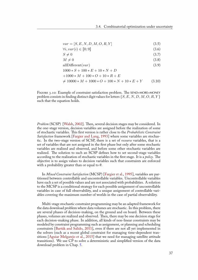
3.4. Combinatorial optimization under uncertainty
var = [S, E, N, D, M, O, R, Y ] (3.5)∀i, var(i) ∈ J0; 9K (3.6)S = 0 (3.7)M = 0 (3.8)allDifferent(var) (3.9)1000 ∗ S + 100 ∗ E + 10 ∗N + D
+1000 ∗M + 100 ∗O + 10 ∗R + E
= 10000 ∗M + 1000 ∗O + 100 ∗N + 10 ∗ E + Y (3.10)
F . : Example of constraint satisfaction problem. e SEND+MORE=MONEYproblem consists in nding distinct digit values for letters S, E, N, D, M, O, R, Y such that the equation holds.
Problem (SCSP) [Walsh, 2002]. en, several decision stages may be considered. Inthe one-stage version, decision variables are assigned before the realization of someof stochastic variables. is rst version is rather close to the Probabilistic ConstraintSatisfaction framework [Fargier and Lang, 1993] where some variables are stochas-tic. In the two-stage version of SCSP, there is a set of recourse variables, that is aset of variables that are not assigned in the rst phase but only after some stochasticvariables are realized and observed, and before some other stochastic variables arerealized. e solution to such an SCSP de nes how to set second-stage variablesaccording to the realization of stochastic variables in the rst stage. It is a policy. eobjective is to assign values to decision variables such that constraints are enforcedwith a probability greater than or equal to θ.
In Mixed Constraint Satisfaction (MCSP) [Fargier et al., 1995], variables are par-titioned between controllable and uncontrollable variables. Uncontrollable variableshave each a set of possible values and are not associated with probabilities. A solutionto the MCSP is a conditional strategy for each possible assignment of uncontrollablevariables in case of full observability, and a unique assignment of controllable vari-ables covering the maximum number of worlds in the case of partial observability.
Multi-stage stochastic constraint programming may be an adapted framework forthe data download problem where data volumes are stochastic. In this problem, thereare several phases of decision-making, on the ground and on board. Between thesephases, volumes are realized and observed. en, there may be one decision stage foreach decision-making phase. In addition, all kinds of non-linear constraints may bemodeled by constraint programming such as assignment, or planning and schedulingconstraints [Barták and Salido, 2011], even if there are not all yet implemented inthe solvers (such as a recent global constraint for managing time-dependent tran-sitions [Aguiar Melgarejo et al., 2015] that we need for managing satellite attitudetransitions). We use CP to solve a deterministic and simpli ed version of the datadownload problem in Chap. 5.
37

. C
3.4.2 Online stochastic combinatorial optimizationOnline Stochastic Combinatorial Optimization (OSCO) is an heuristic online
decision-making framework for problems where data is not available a priori butrevealed during execution [Hentenryck and Bent, 2009]. Targeted problems are forexample those with requests that must be dispatched. e problem consists in choos-ing which request to deal with to maximize utility. OSCO inherits of both onlinemethods, because the objective is to make a decision in a limited time and becausethe uncertainty lies only on the future, and stochastic optimization because samplingis used for decision-making.
Generic offline problem e framework assumes a discrete model of time andconsiders a time horizon H = [1, h]. e input is a sequence ⟨R1, . . . , Rh⟩where each Ri is a set of requests. A solution to the offline problem serves a re-quest r ∈ R1 ∪ . . . ∪ Rt at each time t ∈ H and is represented as a sequenceS = ⟨r1, . . . , rh⟩. is sequence must satisfy the problem-speci c constraints C(C(S) is true in this case) and as each request r ∈ R is associated with a rewardw(r) ≥ 0, w(S) is the reward of the sequence. It is assumed that an algorithm Oable to optimally solve this offline problem is available.
Generic online problem In the online version of the problem, the set of requests⟨R1, . . . , Rh⟩ are not available initially but are revealed progressively at each timestep t. At step t, the online algorithm has at its disposal the sequences ⟨R1, . . . , Rt⟩and the already served requests ⟨s1, . . . , st−1⟩. e goal is to decide which requestto serve. In this online version, the sets of requests ⟨R1, . . . , Rh⟩ are the realizationof random variables ⟨ξ1, . . . , ξh⟩ whose distribution is speci ed by I.
To solve the online stochastic problem, the online algorithms has two back-boxes:1. an offline optimization algorithm O which, given a set of past decisions and
sequence of requests, returns an optimal solution to the problem;2. a conditional sampling procedure S which given a time t and a sampling
horizon ∆, returns a sequence of
S (t, ∆) = ⟨Rt+1, . . . , Rt+∆⟩ (3.11)
realization of the random variables obtained by sampling distribution I.
Algorithm 1: O O (H)1 S0 = ⟨⟩;2 for t ∈ H do3 do st = C R (St−1, ⟨R1, . . . , Rt⟩);4 St → St−1 : st;
e generic online algorithm is shown in Algorithm 1. Different versions ofC R exist as maximizing expectation or hedging against the worst-casescenario. In the following, we only present one version of this procedure in Algo-rithm 2, the Online Expectation (C R -E) version, which is appropriatewhen time constraints are loose. At each time step, it evaluates all possible decisions
38
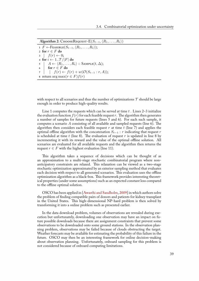
3.4. Combinatorial optimization under uncertainty
Algorithm 2: C R -E(St−1, ⟨R1, . . . , Rt⟩)1 F ←F (St−1, ⟨R1, . . . , Rt⟩);2 for r ∈ F do3 f(r)← 0;4 for i← 1..T /|F | do5 A← ⟨R1, . . . , Rt⟩ :: S (t, ∆);6 for r ∈ F do7 f(r)← f(r) + w(O(St−1 : r, A));8 return arg max(r ∈ F )f(r)
with respect to all scenarios and thus the number of optimizations T should be largeenough in order to produce high-quality results.
Line 1 computes the requests which can be served at time t . Lines 2–3 initializethe evaluation function f(r) for each feasible request r. e algorithm then generatesa number of samples for future requests (lines 5 and 6). For each such sample, itcomputes a scenario A consisting of all available and sampled requests (line 6). ealgorithm then considers each feasible request r at time t (line 7) and applies theoptimal offline algorithm with the concatenation St−1 : r indicating that request ris scheduled at time t (line 8). e evaluation of request r is updated in line 8 byincrementing it with its reward and the value of the optimal offline solution. Allscenarios are evaluated for all available requests and the algorithm then returns therequest r ∈ F with the highest evaluation (line 11).
is algorithm takes a sequence of decisions which can be thought of asan approximation to a multi-stage stochastic combinatorial program where non-anticipatory constraints are relaxed. is relaxation can be viewed as a two-stagestochastic optimization approximated by an exterior sampling method that evaluateseach decision with respect to all generated scenarios. is evaluation uses the offlineoptimization algorithm as a black-box. is framework provides interesting theoret-ical properties (under some assumptions) such as an expected constant loss comparedto the offline optimal solution.
OSCO has been applied in [Awasthi and Sandholm, 2009] in which authors solvethe problem of nding compatible pairs of donors and patients for kidney transplantin the United States. is high-dimensional NP-hard problem is then solved bytransforming it into a online problem such as presented earlier.
In the data download problem, volumes of observations are revealed during exe-cution but unfortunately, downloading one observation may have an impact on fu-ture possible downloads because there are assignment constraints that prevent someobservations to be downloaded onto some ground stations. In the observation plan-ning problem, observations may be failed because of clouds obstructing the target.Weather forecasts may be available for estimating the probability of this failure in thefuture. OSCO may then be an interesting framework for online decision-makingabout observation planning. Unfortunately, onboard sampling for this problem isnot considered because of onboard computing limitations.
39

. C
3.5 Planning and scheduling in the space domainWe have seen how to handle uncertainty for planning and scheduling in general
and now we focus on how these problems are solved in the space domain.Scheduling observations for an Earth-observing satellite is a complex problem :
scientists from several domains need a lot of acquisitions; possible windows to acquiredata are small; ground reception station must communicate with a lot of satellite atthe same time. In that case, the planner may not be able to make the best decisionand human operators often need to validate the automatically generated plans. In-deed, while used by the planning system, information from different sources are ag-gregated and decision-making may sometimes be hardly understandable by humans.Bringing automated tools to operators is difficult and interactive software allow theusers to modify information after visualizing a plan as in the Mixed-Initiative Plan-ning approach [Ai-Chang et al., 2004] which is used for martians rovers Spirit andOpportunity.
Problems from the space domain feature speci c constraints and large searchspaces. Solving these problems often involves new methods. In [Woods et al.,2009b], planning and scheduling techniques are implemented onto a ExoMars pro-totype so it is able to perform autonomous science on Mars. In [Frank et al., 2001],authors present the satellite domain and implement an algorithm based on a heuris-tic tree exploring mechanism called Heuristic Biased Stochastic Sampling [Bresina,1996]. is technique has originally been developed for scheduling observationson telescopes. Pemberton [Pemberton and Greenwald, 2002] proposes an algorithmcombining separation and evaluation with a greedy search for a acquisition schedul-ing problem in which acquisitions have priorities and xed durations. Wolfe andSorensen [Wolfe and Sorensen, 2000] solve a harder problem in which each activityhas an earliest start date, a latest end date, a minimum duration and a maximum du-ration (window-constrained packing problem). ey compare two greedy algorithmswith a genetic algorithm, which is proven to be the best.
Authors of [Lemaître et al., 2002] and [Verfaillie and Lemaître, 2001] are in-terested in scheduling observations on an agile Earth-observing satellite with con-straints close to ours. ey compare four approaches : a greedy algorithm, a dynamicprogramming strategy, constraint programming and local search. e latter presentsthe best performance.
In [Pralet and Verfaillie, 2008], the satellite Frankie of the Hotspot mission mustdetect ground phenomena such as volcanic eruptions or forest res. Onboard plan-ning is done with an anytime iterated stochastic greedy algorithm.
Space systems are expensive and critical resources that are used at their fullpotential. Users send a lot more observation requests than the system is able toprocess. at is why the resulting planning and scheduling resulting problems aresaid to be oversubscribed. Oversubscribed scheduling (OS) is a particular case ofscheduling. In that class of problem, there are not enough resources to processall the tasks. e problem then becomes a lot more difficult since it is not onlya scheduling problem, in which we must decide when tasks are processed and onwhich resources, but also a selection problem, in which we must select rst thebest subset of tasks to be processed. e problem of scheduling for the Air Forcecommunication satellites is studied in [Barbulescu et al., 2006]. Notably, an analysisshows that search spaces of OS problems seem to have large plateaus. is resultleads to design algorithms making large leaps in the search space to escape theseplateaus. In [Globus et al., 2004b], authors had already glimpsed this result bycomparing algorithms on a 2-satellite problem where hill climbing was much worse
40

3.5. Planning and scheduling in the space domain
than simulated annealing. Learning from this fact, we use a large neighborhoodsearch to compute data download plans in Sect. 5.3.
We have seen that planning and scheduling under uncertainty can be tackledwith various frameworks and methods. e challenge, in our case, is the size of theinstances, and many of the methods are not scalable to the thousands of tasks thatacquisition planning or data download scheduling problems include. In the next part,we will focus on the data download problem and provide a model, algorithms, and aexible decision-making approach for this problem.
41

Part II
Building adaptable data downloadschedules
43


IntroductionBecause of the use of more and more sophisticated compression algorithms, the
amount of data that results from an observation and thus is recorded on board andmust be downloaded to the ground is more and more unpredictable. It depends onthe data that has been acquired. In the case of optical instruments, the presenceof clouds over the observed area allows high compression rates and results in a lowamount of data to be recorded and downloaded.
As satellites are not continuously accessible by a ground control station, gener-ated volumes which are directly known on board are available on the ground onlywith some delay. is leads to think that decisions about downloads should be madeon board just before any reception station visibility window with the exact knowl-edge of the volumes of the already recorded data. is approach has been exploredin [Pralet et al., 2014c]. However, planning onboard is time-consuming. Moreover,the resulting plans are unpredictable. is is problematic especially for high-priorityobservations, because users who request an image may want to know when data willbe downloaded. In such conditions, it is still possible to build data download plans onthe ground with the assumption of maximum volumes (minimum default compres-sion rate). e resulting plans are then always executable on board, but suboptimaldue to an under-use of the station visibility windows.
In the work we present in this part, we want to introduce more autonomy onboard satellites while keeping some predictability. e main idea is to share decision-making between ground and board to take advantage of the high computing poweron the ground and of the low uncertainty on board.
First, we provide a model of the data download problem and analyze it. It isa complex scheduling problem with temporal and non-temporal constraints, closeto RCPSP/max or exible job-shop problems. We then design algorithms for thedeterministic version of the problem. We nally propose a exible decision-makingscheme to deal with this problem.
is part of the work has been presented at the following international and nationalconferences : ICAPS’14 [Pralet et al., 2014c], ICAPS’15 [Maillard et al., 2015a],i-SAIRAS’14 [Maillard et al., 2014], JFPC’14 [Pralet et al., 2014a], ROADEF’14,and ROADEF’15. A paper concerning exible scheduling for the data downloadproblem has been accepted for publication in the AIAA J AI S . A paper developing theoretical aspects of the le schedul-ing subproblem is currently being reviewed for publication in D AM .

e Data Download Problem 4
4.1 Informal description . . . . . . . . . . . . . . . . . . . . . 454.2 Formal model of the data download scheduling problem . . . 48
4.2.1 Problem data . . . . . . . . . . . . . . . . . . . . 484.2.2 Decision variables . . . . . . . . . . . . . . . . . . 504.2.3 Constraints . . . . . . . . . . . . . . . . . . . . . 524.2.4 Optimization criterion . . . . . . . . . . . . . . . . 564.2.5 Problem analysis . . . . . . . . . . . . . . . . . . . 594.2.6 Related works . . . . . . . . . . . . . . . . . . . . 60
As seen in Chap. 2, after the satellite has acquired data, it must download it dur-ing ground station visibility windows. In this chapter we formalize the problem ofbuilding an observation download schedule. Note that this problem involves real-lifeconstraints that are harder to tackle than a theoretical combinatorial optimizationproblem. Finding an appropriate way to present these aspects in a complete modelis a challenge. First, we give an informal description of the problem. en, we give aformal model including input data, decision variables, constraints, and an optimiza-tion criterion. Finally, we make some comments on the problem nature and pointsome related works. In the remainder of this manuscript, the words observation andacquisition on one hand, and download window and visibility window on the otherhand, refer to the same concept.
4.1 Informal descriptionTo build a download schedule, decisions must be made at three levels:1. observation download selection, assignment, and scheduling: this consists in
deciding which observations will be downloaded and in building a sequence ofobservation downloads, each download being made of an observation o and ofa download window w assigned to o; this problem is close to a Multi-knapsackproblem [Kellerer et al., 2004] where objects are observations and sacks arewindows, but rst sacks are preferred as freshness of information has to bemaximized, and con icts may exist between sacks (overlapping windows);
2. le download assignment and scheduling: each observation generates severalles; once an observation has been assigned to a download window, this sub-
problem consists in assigning each le of this observation to be downloadedan emission channel, and in building on each channel and on each memorybank a sequence of le downloads; in each download window, the schedul-ing problem is close to a Flexible Open-shop Scheduling problem [Pinedo, 2012]with two types of unsharable resources: channels and memory banks; each ledownload requires one resource of each type, but the choice of the channel isfree, whereas the bank is pre-allocated; the le download order is also free;
3. time management: this consists either in computing earliest and latest datesfor all the events, or in setting their precise dates; the events are the start and
47
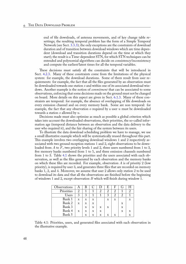
. T D D P
end of le downloads, of antenna movements, and of key change table re-settings; the resulting temporal problem has the form of a Simple TemporalNetwork (see Sect. 3.3.3); the only exceptions are the constraints of downloadduration and of transition between download windows which are time depen-dent (download and transition durations depend on the time at which theystart); the result is a Time-dependent STN, for which STN techniques can beextended and polynomial algorithms can decide on consistency/inconsistencyand compute the earliest/latest times for all the temporal variables.ese decisions must satisfy all the constraints that will be introduced in
Sect. 4.2.3. Many of these constraints come from the limitations of the physicalsystem: for example, the download durations. Some of them result from user re-quirements: for example, the fact that all the les generated by an observation mustbe downloaded towards one station s and within one of its associated download win-dows. Another example is the notion of commitment that can be associated to someobservations, enforcing that some decisions made on the ground must not be changedon board. More details on this aspect are given in Sect. 6.1.3. Many of these con-straints are temporal: for example, the absence of overlapping of le downloads onevery emission channel and on every memory bank. Some are non temporal: forexample, the fact that any observation o required by a user u must be downloadedtowards a station s allowed by u.
Decisions made must also optimize as much as possible a global criterion whichtakes into account the downloaded observations, their priorities, the so-called infor-mation age (temporal distance between an observation and the data delivery to theuser who required it), and the fair sharing of the system between its users.
To illustrate the data download scheduling problem we have to manage, we usea small illustrative example which will be systematically reused throughout this part.
is example involves two overlapping download windows 1 and 2 respectively as-sociated with two ground reception stations 1 and 2, eight observations to be down-loaded from A to F , two priority levels 1 and 2, three users numbered from 1 to 3,ve memory banks numbered from 1 to 5, and three emission channels numbered
from 1 to 3. Table 4.1 shows the priorities and the users associated with each ob-servation, as well as the les generated by each observation and the memory bankson which these les are recorded. For example, observation A is of priority 2 (lowpriority), is required by user 3, and generates three les that are recorded on memorybanks 1, 2, and 4. Moreover, we assume that user 2 allows only station 2 to be usedto download its data and that all the observations are nished before the beginningof windows 1 and 2, except observation B which will nish during window 1.
Observations A B C D E F G HPriorities 2 1 1 2 2 2 1 2
Users 3 3 1 1 3 2 2 1Bank 1 x x x x x xBank 2 x x x xBank 3 x x x x xBank 4 x x x x x xBank 5 x x x x x x
Table 4.1: Priorities, users, and generated les associated with each observation inthe illustrative example.
48

4.1. Informal description
Fig. 4.1 shows a possible download schedule and all its associated temporal con-straints. In this schedule, the sequence of observation downloads is C, H, B, G, Ewith observations C, H , and B downloaded in window 1 and observations G and Edownloaded in window 2. Observations A, D, and F are not downloaded (they willbe downloaded later). If we go down at the le level, we see on which channel andin which order the several les generated by an observation are downloaded: for ex-ample for observation C, le recorded in bank 4 ((C, 4)) on channel 1, les recordedin banks 2 and 5 ((C, 2) and (C, 5)) in sequence on channel 2, and les recorded inbanks 1 and 3 ((C, 1) and (C, 3)) in sequence on channel 3.
All the temporal constraints that result from this schedule are represented inFig. 4.1:
1. channel precedence constraints: these constraints express the fact there mustbe no overlapping between le downloads on the same channel; for example,the download of (C, 2) must precede the download of (C, 5) on channel 2;
2. memory bank precedence constraints: they express the fact there must be nooverlapping between le downloads from the same memory bank; for example,the download of (H, 4) must precede the download of (B, 4) because both arerecorded on the same bank;
3. acquisition precedence constraints: they express the fact that no observationcan be downloaded before being nished; for example, the download of (B, 4)cannot start before t1 which is assumed to be the end time of observation B(start and end of observations are provided by the observation schedule);
4. window precedence constraints: they express the fact that all the le downloadsassociated with an observation o must be included in the window assigned too; for example, the download of (G, 3) must start after the start time s2 ofwindow 2 and the download of (E, 3) must end before the end time e2 of thesame window;
5. antenna move transition constraints: they express the fact that moving the mo-bile emission antenna from a station to another one takes some time duringwhich no download is possible; for example, a minimum distance is requiredbetween the end of download of (B, 5) and the start of download of (G, 2);such a distance depends on both stations and on the time at which the transi-tion starts (time-dependent transition time);
6. table resetting transition constraints: they express the fact that resetting thekey change table used for encrypting user data takes some time during whichno download is possible; for example, because we assume that we take advan-tage of the antenna movement to reset the key change table, another minimumconstant distance is required between the end of download of (B, 5) and thestart of download of (G, 2);
7. le download duration constraints: they are represented in the gure by thelengths of the rectangles associated with each le download; because thedownload rate is not constant over a download window and depends on thesatellite-station distance, download durations depend on the time at whichthey start (time-dependent duration).
Fig. 4.2 shows the associated earliest schedule where all the downloads are sched-uled as soon as possible.
49
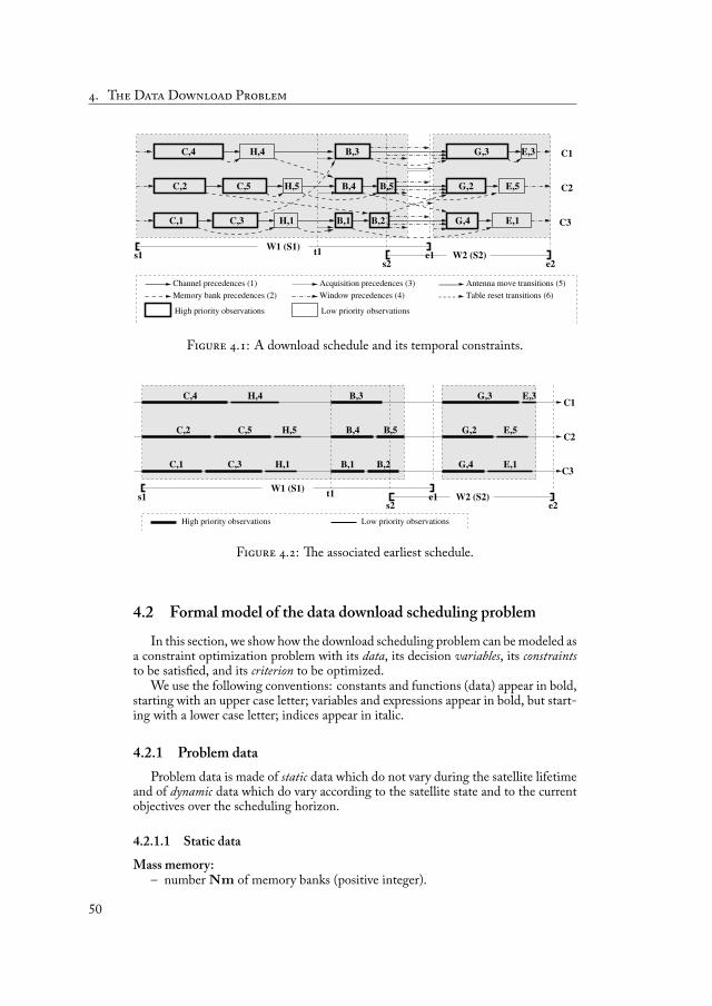
. T D D P
C1
C3
C,4
C2
C,1
C,5C,2
H,4
H,5
C,3
B,3
B,4
H,1
B,5
B,2B,1
G,2
G,4
G,3
E,5
E,1
E,3
e1s1W1 (S1)
e2s2W2 (S2)
Channel precedences (1)
Memory bank precedences (2)
t1
Window precedences (4)
Antenna move transitions (5)Acquisition precedences (3)
High priority observations Low priority observations
Table reset transitions (6)
F . : A download schedule and its temporal constraints.
High priority observations Low priority observations
B,3
B,1
B,5B,4C2
C3
C1E,3G,3
B,2 E,1
G,2 E,5
C,4 H,4
G,4
C,5 H,5C,2
C,3 H,1C,1
W2 (S2)e2
W1 (S1)s1
s2e1t1
F . : e associated earliest schedule.
4.2 Formal model of the data download scheduling problemIn this section, we show how the download scheduling problem can be modeled as
a constraint optimization problem with its data, its decision variables, its constraintsto be satis ed, and its criterion to be optimized.
We use the following conventions: constants and functions (data) appear in bold,starting with an upper case letter; variables and expressions appear in bold, but start-ing with a lower case letter; indices appear in italic.
4.2.1 Problem dataProblem data is made of static data which do not vary during the satellite lifetime
and of dynamic data which do vary according to the satellite state and to the currentobjectives over the scheduling horizon.
4.2.1.1 Static dataMass memory:
– number Nm of memory banks (positive integer).
50

4.2. Formal model of the data download scheduling problem
– capacity Cm of each memory bank (positive integer).
Emission antenna:– number Nc of emission channels (positive integer);– angular velocity Sa of the orientable antenna (positive oat).
Data encryption:– maximum number Nkmax of changes per channel that can be recorded in
the key change table (positive integer);– duration DuKct required to reset the key change table (positive oat).
Ground reception stations:– number Ns of ground reception stations (positive integer).
Users:– number Nu of users of the system (positive integer);– for each user u ∈ J1, NuK and each reception station s ∈ J1, NsK,
– a boolean Alls,u indicating whether or not data required by user u may bedownloaded towards station s;
– a data transfer rate Gtrs,u on the ground from s to the processing center ofu (positive oat).
Priorities:– number Np of priority levels (positive integer).
4.2.1.2 Dynamic dataScheduling horizon:
– Ts: start time of the download scheduling horizon (positive oat);– Te: end time of the download scheduling horizon (positive oat).
Download windows:– number Nw of (effective) download windows over the scheduling horizon
(positive integer); these windows are computed from the ground reception sta-tion visibility windows and from the observation schedule and the associatedsatellite attitude trajectory;
– for each download window w ∈ J1, NwK:– a start time Sww (positive oat);– an end time Eww (positive oat);– an associated reception station Stw (integer in J1, NsK);– a function Drw : [Sww, Eww] → R+ which gives the download rate
within download window w as a function of time; function Drw is assumedto be piecewise constant.
Observations:– number No of observations that can be downloaded over the scheduling hori-
zon (positive integer): observations that have been already performed but notdownloaded yet and observations that have been not performed yet, but arescheduled (present in the observation schedule);
51
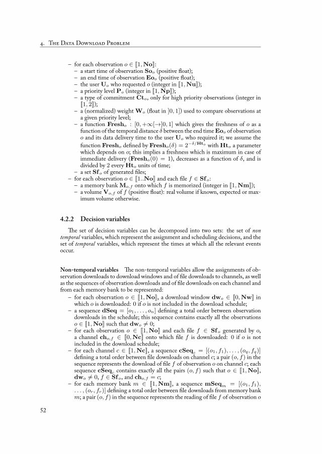
. T D D P
– for each observation o ∈ J1, NoK:– a start time of observation Soo (positive oat);– an end time of observation Eoo (positive oat);– the user Uo who requested o (integer in J1, NuK);– a priority level Po (integer in J1, NpK);– a type of commitment Cto, only for high priority observations (integer inJ1, 2K);– a (normalized) weight Wo ( oat in ]0, 1]) used to compare observations at
a given priority level;– a function Fresho : [0, +∞[→]0, 1] which gives the freshness of o as a
function of the temporal distance δ between the end time Eoo of observationo and its data delivery time to the user Uo who required it; we assume thefunction Fresho de ned by Fresho(δ) = 2−δ/Hto with Hto a parameterwhich depends on o; this implies a freshness which is maximum in case ofimmediate delivery (Fresho(0) = 1), decreases as a function of δ, and isdivided by 2 every Hto units of time;
– a set Sfo of generated les;– for each observation o ∈ J1..NoK and each le f ∈ Sf o:
– a memory bank Mo,f onto which f is memorized (integer in J1, NmK);– a volume Vo,f of f (positive oat): real volume if known, expected or max-
imum volume otherwise.
4.2.2 Decision variablese set of decision variables can be decomposed into two sets: the set of non
temporal variables, which represent the assignment and scheduling decisions, and theset of temporal variables, which represent the times at which all the relevant eventsoccur.
Non-temporal variables e non-temporal variables allow the assignments of ob-servation downloads to download windows and of le downloads to channels, as wellas the sequences of observation downloads and of le downloads on each channel andfrom each memory bank to be represented:
– for each observation o ∈ J1, NoK, a download window dwo ∈ J0, NwK inwhich o is downloaded: 0 if o is not included in the download schedule;
– a sequence dSeq = [o1, . . . , on] de ning a total order between observationdownloads in the schedule; this sequence contains exactly all the observationso ∈ J1, NoK such that dwo = 0;
– for each observation o ∈ J1, NoK and each le f ∈ Sf o generated by o,a channel cho,f ∈ J0, NcK onto which le f is downloaded: 0 if o is notincluded in the download schedule;
– for each channel c ∈ J1, NcK, a sequence cSeqc = [(o1, f1), . . . , (oq, fq)]de ning a total order between le downloads on channel c; a pair (o, f) in thesequence represents the download of le f of observation o on channel c; eachsequence cSeqc contains exactly all the pairs (o, f) such that o ∈ J1, NoK,dwo = 0, f ∈ Sfo, and cho,f = c;
– for each memory bank m ∈ J1, NmK, a sequence mSeqm = [(o1, f1),. . . , (or, fr)] de ning a total order between le downloads from memory bankm; a pair (o, f) in the sequence represents the reading of le f of observation o
52
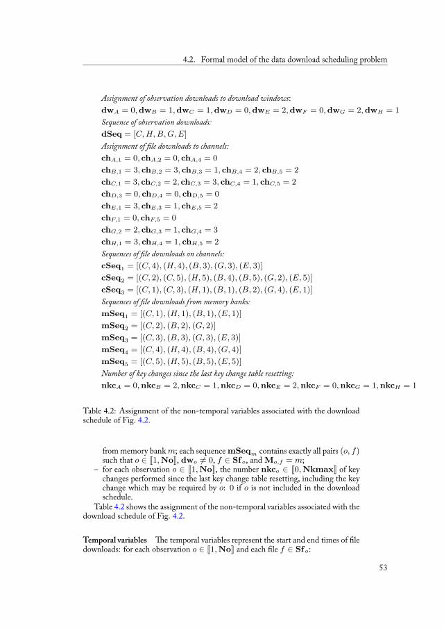
4.2. Formal model of the data download scheduling problem
Assignment of observation downloads to download windows:dwA = 0, dwB = 1, dwC = 1, dwD = 0, dwE = 2, dwF = 0, dwG = 2, dwH = 1Sequence of observation downloads:dSeq = [C, H, B, G, E]Assignment of le downloads to channels:chA,1 = 0, chA,2 = 0, chA,4 = 0chB,1 = 3, chB,2 = 3, chB,3 = 1, chB,4 = 2, chB,5 = 2chC,1 = 3, chC,2 = 2, chC,3 = 3, chC,4 = 1, chC,5 = 2chD,3 = 0, chD,4 = 0, chD,5 = 0chE,1 = 3, chE,3 = 1, chE,5 = 2chF,1 = 0, chF,5 = 0chG,2 = 2, chG,3 = 1, chG,4 = 3chH,1 = 3, chH,4 = 1, chH,5 = 2Sequences of le downloads on channels:cSeq1 = [(C, 4), (H, 4), (B, 3), (G, 3), (E, 3)]cSeq2 = [(C, 2), (C, 5), (H, 5), (B, 4), (B, 5), (G, 2), (E, 5)]cSeq3 = [(C, 1), (C, 3), (H, 1), (B, 1), (B, 2), (G, 4), (E, 1)]Sequences of le downloads from memory banks:mSeq1 = [(C, 1), (H, 1), (B, 1), (E, 1)]mSeq2 = [(C, 2), (B, 2), (G, 2)]mSeq3 = [(C, 3), (B, 3), (G, 3), (E, 3)]mSeq4 = [(C, 4), (H, 4), (B, 4), (G, 4)]mSeq5 = [(C, 5), (H, 5), (B, 5), (E, 5)]Number of key changes since the last key change table resetting:nkcA = 0, nkcB = 2, nkcC = 1, nkcD = 0, nkcE = 2, nkcF = 0, nkcG = 1, nkcH = 1
Table 4.2: Assignment of the non-temporal variables associated with the downloadschedule of Fig. 4.2.
from memory bank m; each sequence mSeqm contains exactly all pairs (o, f)such that o ∈ J1, NoK, dwo = 0, f ∈ Sfo, and Mo,f = m;
– for each observation o ∈ J1, NoK, the number nkco ∈ J0, NkmaxK of keychanges performed since the last key change table resetting, including the keychange which may be required by o: 0 if o is not included in the downloadschedule.
Table 4.2 shows the assignment of the non-temporal variables associated with thedownload schedule of Fig. 4.2.
Temporal variables e temporal variables represent the start and end times of ledownloads: for each observation o ∈ J1, NoK and each le f ∈ Sfo:
53
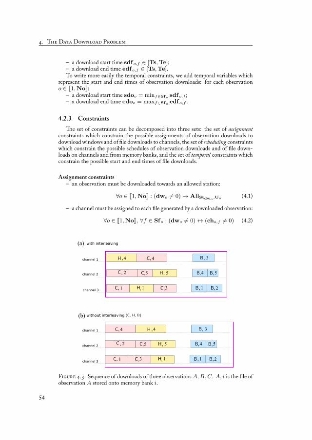
. T D D P
– a download start time sdf o,f ∈ [Ts, Te];– a download end time edfo,f ∈ [Ts, Te].To write more easily the temporal constraints, we add temporal variables which
represent the start and end times of observation downloads: for each observationo ∈ J1, NoK:
– a download start time sdoo = minf∈Sfo sdf o,f ;– a download end time edoo = maxf∈Sfo edf o,f .
4.2.3 Constraintse set of constraints can be decomposed into three sets: the set of assignment
constraints which constrain the possible assignments of observation downloads todownload windows and of le downloads to channels, the set of scheduling constraintswhich constrain the possible schedules of observation downloads and of le down-loads on channels and from memory banks, and the set of temporal constraints whichconstrain the possible start and end times of le downloads.
Assignment constraints– an observation must be downloaded towards an allowed station:
∀o ∈ J1, NoK : (dwo = 0)→ AllStdwo ,Uo (4.1)
– a channel must be assigned to each le generated by a downloaded observation:
∀o ∈ J1, NoK, ∀f ∈ Sf o : (dwo = 0)↔ (cho,f = 0) (4.2)
F . : Sequence of downloads of three observations A, B, C. A, i is the le ofobservation A stored onto memory bank i.
54
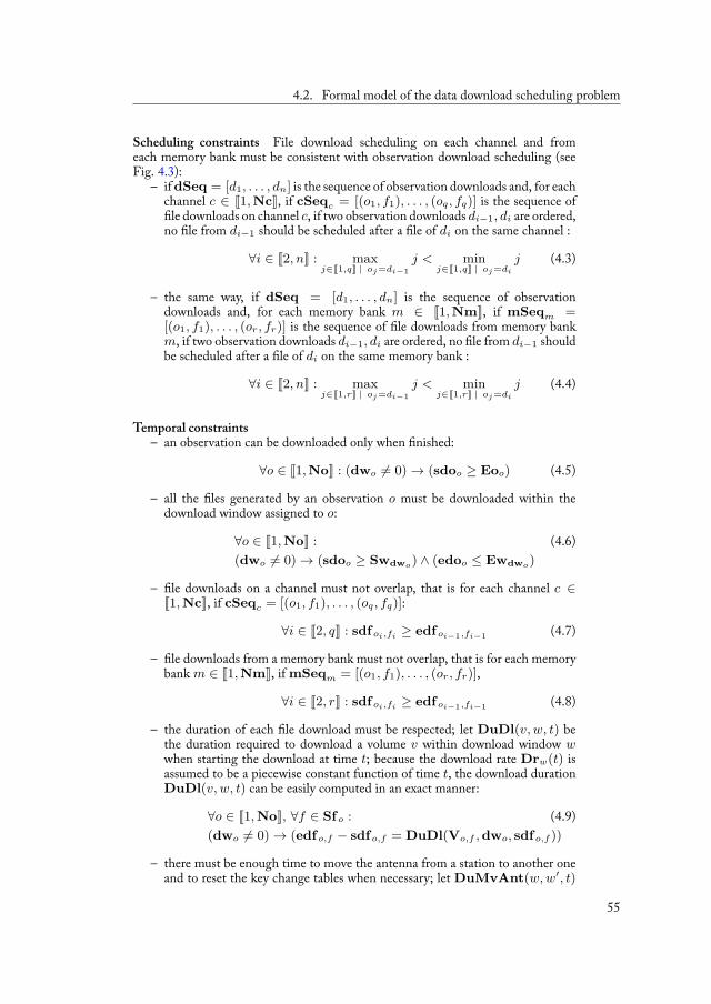
4.2. Formal model of the data download scheduling problem
Scheduling constraints File download scheduling on each channel and fromeach memory bank must be consistent with observation download scheduling (seeFig. 4.3):
– if dSeq = [d1, . . . , dn] is the sequence of observation downloads and, for eachchannel c ∈ J1, NcK, if cSeqc = [(o1, f1), . . . , (oq, fq)] is the sequence ofle downloads on channel c, if two observation downloads di−1, di are ordered,
no le from di−1 should be scheduled after a le of di on the same channel :
∀i ∈ J2, nK : maxj∈J1,qK | oj =di−1
j < minj∈J1,qK | oj =di
j (4.3)
– the same way, if dSeq = [d1, . . . , dn] is the sequence of observationdownloads and, for each memory bank m ∈ J1, NmK, if mSeqm =[(o1, f1), . . . , (or, fr)] is the sequence of le downloads from memory bankm, if two observation downloads di−1, di are ordered, no le from di−1 shouldbe scheduled after a le of di on the same memory bank :
∀i ∈ J2, nK : maxj∈J1,rK | oj =di−1
j < minj∈J1,rK | oj =di
j (4.4)
Temporal constraints– an observation can be downloaded only when nished:
∀o ∈ J1, NoK : (dwo = 0)→ (sdoo ≥ Eoo) (4.5)
– all the les generated by an observation o must be downloaded within thedownload window assigned to o:
∀o ∈ J1, NoK : (4.6)(dwo = 0)→ (sdoo ≥ Swdwo ) ∧ (edoo ≤ Ewdwo )
– le downloads on a channel must not overlap, that is for each channel c ∈J1, NcK, if cSeqc = [(o1, f1), . . . , (oq, fq)]:
∀i ∈ J2, qK : sdf oi,fi ≥ edf oi−1,fi−1 (4.7)
– le downloads from a memory bank must not overlap, that is for each memorybank m ∈ J1, NmK, if mSeqm = [(o1, f1), . . . , (or, fr)],
∀i ∈ J2, rK : sdf oi,fi ≥ edf oi−1,fi−1 (4.8)
– the duration of each le download must be respected; let DuDl(v, w, t) bethe duration required to download a volume v within download window wwhen starting the download at time t; because the download rate Drw(t) isassumed to be a piecewise constant function of time t, the download durationDuDl(v, w, t) can be easily computed in an exact manner:
∀o ∈ J1, NoK, ∀f ∈ Sf o : (4.9)(dwo = 0)→ (edfo,f − sdf o,f = DuDl(Vo,f , dwo, sdf o,f ))
– there must be enough time to move the antenna from a station to another oneand to reset the key change tables when necessary; let DuMvAnt(w, w′, t)
55

. T D D P
be the minimum duration required to move from a pointing towards stations associated with download window w to a pointing towards station s′ asso-ciated with download window w′ when starting the movement at time t; aniterative method, similar to the algorithms used to compute satellite attitudemovements in minimum time, is used to compute DuMvAnt(w, w′, t); ifdSeq = [o1, . . . , on] is the sequence of observation downloads:
∀i ∈ J2, nK :(sdooi−1 ≤ sdooi ) ∧ (edooi−1 ≤ edooi ) (4.10)
(dwoi = dwoi−1 )→ ((sdooi − edooi−1 ≥ (4.11)max(DuKct, DuMvAnt(dwoi−1 , dwoi , edooi−1 ))) ∧(nkcoi = 1))
((dwoi = dwoi−1 ) ∧ (Uoi = Uoi−1 ) ∧ (4.12)(nkcoi−1 = Nkmax))→ ((sdooi − edooi−1 ) ≥ DuKct) ∧(nkcoi = 1))
((dwoi = dwoi−1 ) ∧ (Uoi = Uoi−1 ) ∧ (4.13)(nkcoi−1 < Nkmax))→ (nkcoi = nkcoi−1 + 1)((dwoi = dwoi−1 ) ∧ (Uoi = Uoi−1 )
)→ (nkcoi = nkcoi−1 )(4.14)
Constraint 4.10 enforces that two successive observations downloads in the se-quence are actually scheduled in the same order on channels. Constraint 4.11 en-forces that, when two successive observation downloads are not in the same downloadwindow, there must be enough time between the end of the rst download and thestart of the second to move the antenna from the rst station to the second one andto reset the key change table (this reset is performed at each transition to make theproblem easier to solve). e current number of key changes is then reset to 1. atmeans that we take systematically bene t of antenna moves to reset the key changetable. Constraint 4.12 enforces that when two successive observation downloads onthe same download window do not belong to the same user and when the maximumnumber of changes in the table is reached, there must be enough time between theend of the rst download and the start of the second to reset the key change table.
e current number of key changes is then reset to 1. Constraint 4.13 enforces thatwhen two successive observation downloads on the same download window do notbelong to the same user and when the maximum number of changes in the table is notreached, the current number of key changes is incremented. Finally, constraint 4.14enforces that when two successive acquisition downloads on the same download win-dow belong to the same user, the number of key changes remains unchanged. atmeans that we reset the key change table only when necessary.
Computing antenna movement durations e term DuMvAnt(w, w′, t) rep-resents the duration required for the antenna to move from a pointing towards thestation associated with w to a pointing towards the station associated with w′ if
56
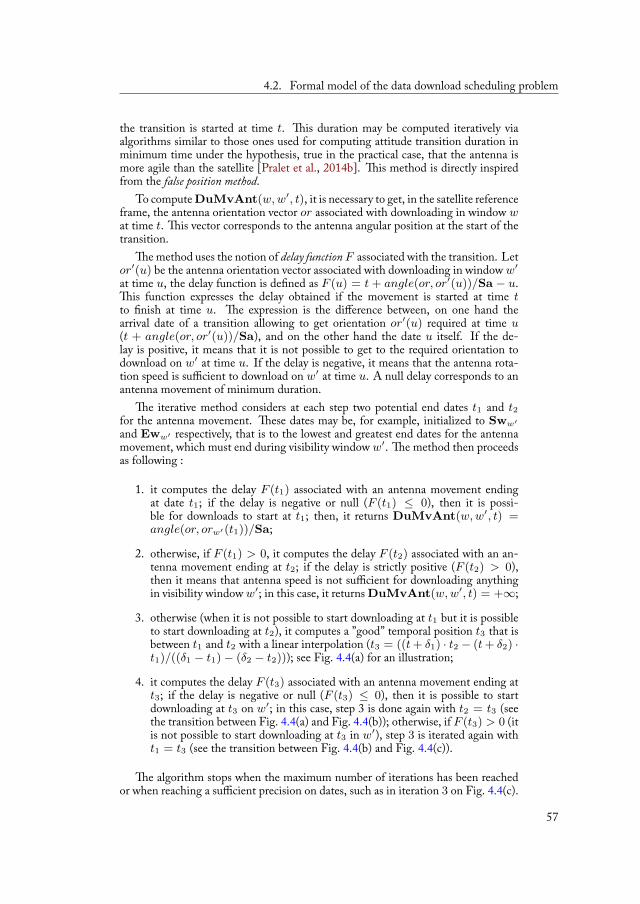
4.2. Formal model of the data download scheduling problem
the transition is started at time t. is duration may be computed iteratively viaalgorithms similar to those ones used for computing attitude transition duration inminimum time under the hypothesis, true in the practical case, that the antenna ismore agile than the satellite [Pralet et al., 2014b]. is method is directly inspiredfrom the false position method.
To compute DuMvAnt(w, w′, t), it is necessary to get, in the satellite referenceframe, the antenna orientation vector or associated with downloading in window wat time t. is vector corresponds to the antenna angular position at the start of thetransition.
e method uses the notion of delay function F associated with the transition. Letor′(u) be the antenna orientation vector associated with downloading in window w′
at time u, the delay function is de ned as F (u) = t + angle(or, or′(u))/Sa − u.is function expresses the delay obtained if the movement is started at time t
to nish at time u. e expression is the difference between, on one hand thearrival date of a transition allowing to get orientation or′(u) required at time u(t + angle(or, or′(u))/Sa), and on the other hand the date u itself. If the de-lay is positive, it means that it is not possible to get to the required orientation todownload on w′ at time u. If the delay is negative, it means that the antenna rota-tion speed is sufficient to download on w′ at time u. A null delay corresponds to anantenna movement of minimum duration.
e iterative method considers at each step two potential end dates t1 and t2for the antenna movement. ese dates may be, for example, initialized to Sww′
and Eww′ respectively, that is to the lowest and greatest end dates for the antennamovement, which must end during visibility window w′. e method then proceedsas following :
1. it computes the delay F (t1) associated with an antenna movement endingat date t1; if the delay is negative or null (F (t1) ≤ 0), then it is possi-ble for downloads to start at t1; then, it returns DuMvAnt(w, w′, t) =angle(or, orw′ (t1))/Sa;
2. otherwise, if F (t1) > 0, it computes the delay F (t2) associated with an an-tenna movement ending at t2; if the delay is strictly positive (F (t2) > 0),then it means that antenna speed is not sufficient for downloading anythingin visibility window w′; in this case, it returns DuMvAnt(w, w′, t) = +∞;
3. otherwise (when it is not possible to start downloading at t1 but it is possibleto start downloading at t2), it computes a ”good” temporal position t3 that isbetween t1 and t2 with a linear interpolation (t3 = ((t + δ1) · t2 − (t + δ2) ·t1)/((δ1 − t1)− (δ2 − t2))); see Fig. 4.4(a) for an illustration;
4. it computes the delay F (t3) associated with an antenna movement ending att3; if the delay is negative or null (F (t3) ≤ 0), then it is possible to startdownloading at t3 on w′; in this case, step 3 is done again with t2 = t3 (seethe transition between Fig. 4.4(a) and Fig. 4.4(b)); otherwise, if F (t3) > 0 (itis not possible to start downloading at t3 in w′), step 3 is iterated again witht1 = t3 (see the transition between Fig. 4.4(b) and Fig. 4.4(c)).
e algorithm stops when the maximum number of iterations has been reachedor when reaching a sufficient precision on dates, such as in iteration 3 on Fig. 4.4(c).
57
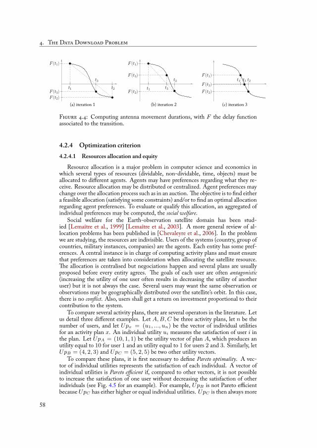
. T D D P
t3
t1F (t3)
t2
F (t2)
F (t1)
t2
t3t1F (t2)
F (t3)
F (t1)
F (t1)
F (t3)F (t2)
t3 t2t1
(c) iteration 3(b) iteration 2(a) iteration 1
F . : Computing antenna movement durations, with F the delay functionassociated to the transition.
4.2.4 Optimization criterion4.2.4.1 Resources allocation and equity
Resource allocation is a major problem in computer science and economics inwhich several types of resources (dividable, non-dividable, time, objects) must beallocated to different agents. Agents may have preferences regarding what they re-ceive. Resource allocation may be distributed or centralized. Agent preferences maychange over the allocation process such as in an auction. e objective is to nd eithera feasible allocation (satisfying some constraints) and/or to nd an optimal allocationregarding agent preferences. To evaluate or qualify this allocation, an aggregated ofindividual preferences may be computed, the social welfare.
Social welfare for the Earth-observation satellite domain has been stud-ied [Lemaître et al., 1999] [Lemaître et al., 2003]. A more general review of al-location problems has been published in [Chevaleyre et al., 2006]. In the problemwe are studying, the resources are indivisible. Users of the systems (country, group ofcountries, military instances, companies) are the agents. Each entity has some pref-erences. A central instance is in charge of computing activity plans and must ensurethat preferences are taken into consideration when allocating the satellite resource.
e allocation is centralised but negociations happen and several plans are usuallyproposed before every entity agrees. e goals of each user are often antagonistic(increasing the utility of one user often results in decreasing the utility of anotheruser) but it is not always the case. Several users may want the same observation orobservations may be geographically distributed over the satellite’s orbit. In this case,there is no con ict. Also, users shall get a return on investment proportional to theircontribution to the system.
To compare several activity plans, there are several operators in the literature. Letus detail three different examples. Let A, B, C be three activity plans, let n be thenumber of users, and let Upx = (u1, ..., un) be the vector of individual utilitiesfor an activity plan x. An individual utility ui measures the satisfaction of user i inthe plan. Let UpA = (10, 1, 1) be the utility vector of plan A, which produces anutility equal to 10 for user 1 and an utility equal to 1 for users 2 and 3. Similarly, letUpB = (4, 2, 3) and UpC = (5, 2, 5) be two other utility vectors.
To compare these plans, it is rst necessary to de ne Pareto optimality. A vec-tor of individual utilities represents the satisfaction of each individual. A vector ofindividual utilities is Pareto efficient if, compared to other vectors, it is not possibleto increase the satisfaction of one user without decreasing the satisfaction of otherindividuals (see Fig. 4.5 for an example). For example, UpB is not Pareto efficientbecause UpC has either higher or equal individual utilities. UpC is then always more
58

4.2. Formal model of the data download scheduling problem
F . : Example of Pareto front for a 2-objective problem. Solutions s1 and s2are on the front because f(s1) > f(s2) and g(s1) < g(s2). All solutions on thePareto front are Pareto-efficient.
interesting, in the sense of Pareto, than UpB . It is generally admitted that an oper-ator choosing a solution among several must choose a Pareto-efficient solution. edifficulty now is to choose a solution among several Pareto-efficient solutions.
Let now compare UpA and UpC with the∑
operator that sums all utilities. Sumis 10 + 1 + 1 = 12 for UpA and 5 + 2 + 5 = 12 for UpC . e
∑operator is said
to be utilitarist, it is Pareto-efficient and does not take into account equity betweenindividuals. If equity matters, the min operator can be used instead to choose thesolution maximizing the minimum individual utility. Unfortunately, it is not Pareto-efficient. If UpB and UpC are compared, minimum individual utilities are equal,this operator may choose UpB which is not Pareto-efficient. e leximin operatoris also favoring equality but is Pareto-efficient. If UpB and UpC are compared,their vectors are rst ordered by increasing individual utility. Vectors (2, 3, 4) and(2, 5, 5) are then lexicographically compared until one individual utility dominatesthe other (here, 5 dominates 3). Here, UpC is chosen. In the following, we presenta criterion which produces these individual utilities and includes a mechanism tosupport utilitarism or egalitarism.
4.2.4.2 Criterion for the Data Download Probleme optimization criterion we consider to discriminate several consistent down-
load schedules (which satisfy all the constraints) takes into account the user prefer-ences (observation priorities and weights), the information age (temporal distancebetween observations and data delivery to the users who required them), and the fairsharing of the system between its users.
Let Π be a xed download schedule where all decision variables (non temporaland temporal) have been set.
We can associate with each observation o ∈ J1, NoK a freshness value fro between0 et 1. is value depends on the temporal distance between the end time Eoo ofobservation o and the time dto at which the last le of o is delivered to the user uthat required o (including the ground transfer duration between the reception station
59
. T D D P
and the data production center of u, which can be estimated via simulation). Moreprecisely, the freshness fro of o is de ned by:
fro =
Fresho(dto −Eoo) = 2(Eoo−dto)/Hto if (dwo = 0)0 otherwise (4.15)
We can now associate with each observation o a corrected weight wco which is theproduct of its (normalized) weight Wo by its freshness fro: wco = Wo · fro. isway, we penalize observations regarding their freshness while taking their weight intoaccount.
In such conditions, we can associate with each priority level p ∈ J1, NpK andeach user u ∈ J1, NuK what we refer to as the individual utility ui(Π, p, u) of thedownload schedule Π at priority level p for user u. is utility is de ned by:
ui(Π, p, u) =
1 if ∃o ∈ J1, NoK | (Po = p) ∧ (Uo = u)∑o∈J1,NoK | (Po=p)∧(Uo=u)
wco otherwise (4.16)
It is equal to the sum of the corrected weights of the observations that are down-loaded in Π and that are of priority p and required by u if any exists. If none exists,it is is equal to 1 (perfect satisfaction because nothing is required). anks to weightnormalization, it takes its value in [0, 1].
e problem is now to aggregate individual utilities. Following [Lemaître et al.,2003], we associate with each priority level p ∈ J1, NpK what we refer to as the socialutility us(Π, p) of the download schedule Π at priority level p. Let Ps be a sharingparameter set in agreement with the system users. is utility is de ned by:
us(Π, p) =
(
1Nu ·
∑u∈J1,NuK (ui(Π, p, u))Ps
)1/Psif Ps = 0 ∏
u∈J1,NuKui(Π, p, u)
1/Nu
if Ps = 0(4.17)
As individual utilities do, it takes its value in [0, 1]. Parameter Ps allows thetrade-off between utilitarism (maximizing the total utility) and egalitarism (allowingevery user to have an equal utility) to be adjusted. When Ps = 1, the social utilityis the mean of the individual utilities: utilitarian approach without equity preoccu-pation. When Ps tends towards −∞, social utility tends towards the minimum ofthe individual utilities: pure egalitarian approach with a high equity preoccupation.Ps = 0 is a compromise between utilitarian and egalitarian approaches.
We can now associate with each download schedule Π a social utility vector wherea social utility is associated with each priority level:
vus(Π) = (us(Π, 1), . . . , us(Π, Np)) (4.18)
Two download schedules Π1 et Π2 can nally be compared by comparing theirassociated social utility vectors in a lexicographic way from the highest to the lowestpriority level. is expresses that any improvement at a priority level is preferred toany improvement at lower priority levels.
60
4.2. Formal model of the data download scheduling problem
4.2.5 Problem analysisMemory capacity e checking of the memory constraint (absence of memoryoverwriting) does not appear in the above download scheduling problem de nition.However, once a download schedule is built, the associated memory pro le can bebuilt and checked. ere are two main justi cations for such a two stage approach.First, thanks to the very high capacity of new generation onboard mass memories,this constraint is rarely violated. Second, the memory pro les that can be built re-main uncertain due to the uncertainty about (1) the actual volumes generated byobservations, (2) the arrival of data reception acknowledgments which allow data tobe removed from the mass memory and (3) the actual download decisions made onboard in the onboard and mixed approaches. is is why we prefer to use the obser-vation execution mechanism that will be presented in Sect. 6.1.2 and prevents anymemory overwriting from happening: if performing an observation o may lead toa memory overwriting, either o is not performed, or lower priority data is removedfrom memory to free space.
Temporal part of the problem It must be stressed that, once all the non temporalvariables have been set, that is once all the assignment and scheduling decisions havebeen made, the remaining part of the problem is made of temporal variables andconstraints. is temporal part has the form of a TSTN (Time-dependent Sim-ple Temporal Network [Pralet and Verfaillie, 2013b]). e TSTN framework is anextension of the STN framework. In the STN framework, all the variables repre-sent temporal positions and all the constraints are binary constraints of the formx − y ≥ d where x and y are variables and d is a constant, referred to as simpletemporal constraints. In the TSTN framework, all the constraints are of the formx − y ≥ d(x, y) where x and y are variables and d is a function of x and y (or ofthe form x − y ≥ d(x) where d is a function of x), referred to as time-dependentsimple temporal constraints.
Constraints from 4.5 to 4.8, as well as Constraint 4.12 are simple temporal con-straints, whereas Constraints 4.9 and 4.11 are time-dependent simple temporal con-straints (time-dependent durations of le downloads and antenna movements).
In [Pralet and Verfaillie, 2013b], it has been proven that the main results es-tablished in the STN framework can be under some assumptions about the formof the distance d functions (e.g. monotonicity, assumption that is satis ed in ourapplication) extended to the TSTN framework: existence of polynomial constraintpropagation algorithms that allow consistency or inconsistency of the TSTN to bedetermined and, in case of consistency, the earliest and latest times of each tempo-ral variable to be computed; consistency of the assignment where all the temporalvariables are set to their earliest time (or to their latest time).
is suggests an algorithmic constraint-based approach where assignment andscheduling decisions are made rst, temporal constraints are then propagated and, incase of consistency (no empty domain of a temporal variable), temporal variables areset to their earliest time in order to minimize information age.
Instance size As we will see in Sect. 6.5.2, the real-world instances we have tomanage involve more than one thousand of observations over each day. As a conse-quence, if we consider only download scheduling decisions (variable dSeq), the sizeof the search space is higher than !1000 (we note that the size of the search spacedoes not imply that the problem is hard as we can prune it). e size of this searchspace and the absence of polynomial scheduling algorithms prevent us from using
61
. T D D P
exact algorithms and suggest the use of approximate algorithms (based on greedy orlocal searches) to make assignment and scheduling decisions and then to propagatethe resulting temporal constraints (time-dependent or not).
4.2.6 Related worksData download planning Whereas the problem of selecting and scheduling obser-vations for Earth observation satellites has been extensively studied (see [Lemaîtreet al., 2002; Globus et al., 2004b] for partial surveys), studies about data downloadplanning are more seldom. e problem of planning (offline on the ground) datadownloads from a Mars orbiter to Earth has been studied in [Oddi et al., 2003;Cesta et al., 2007]. In [Oddi and Policella, 2004; Righini and Tresoldi, 2010], ithas been shown that this problem can be modeled as a Max-Flow problem and thussolved using either Max-Flow or Linear Programming polynomial algorithms. Touse a similar approach in our context, we should linearize the criterion and relax manyconstraints, for example the constraints that enforce that a le download cannot beinterrupted and distributed over several channels or download windows. Hence, aMax-Flow formulation of our problem can only produce upper bounds on the max-imum utility. In the context of the EO-1 experiment [Chien et al., 2004a], obser-vation requests may be generated either by ground users, or autonomously on boardfollowing the detection of ground phenomena such as volcanic eruptions, oods,or ice breakups by onboard data analysis algorithms. In such a context, observa-tion and download plans are built or adapted on board using an iterative repair ap-proach [Chien et al., 2000]: local search algorithms implemented in the genericCASPER planning tool.
Uncertain volumes e situation where the amount of data that is produced andmust be downloaded is variable and uncertain is present in planetary exploration aswell as in Earth observation and surveillance missions. In [Castano et al., 2007]and [Woods et al., 2009a], onboard planning and scheduling (including data down-load planning and scheduling) is studied in order to allow a planetary explorationrover to adapt itself to what it detects. More precisely, in [ ompson et al., 2008],what is downloaded is selected in order to meet download limitations and to maxi-mize the information value that scientists will be able to extract from it. In [Oddi andPolicella, 2004], an iterated procedure is designed to lower lling peaks in memorybanks in order to manage uncertainty about the volumes of data to be downloadedby a Mars orbiter and to limit the risk of memory bank overwriting. In [Righini andTresoldi, 2010], Integer Linear Programming formulations are proposed to addressthis problem. In [Chien et al., 2004a], uncertainty is managed using a reactive it-erative repair planning approach. In [Verfaillie et al., 2011], the operational contextis an electromagnetic Earth surveillance mission where the variability of the gener-ated data volumes is very high. Several mechanisms, especially designed for onboarddownload decision-making, are compared in terms of computing time, number ofdownloads, and window utilization: decision rules, reactive planning, or sampling +planning.
62
Algorithms for the deterministic Data Download PlanningProblem 5
5.1 Exact method: constraint programming . . . . . . . . . . . . 615.2 Greedy algorithms . . . . . . . . . . . . . . . . . . . . . . 64
5.2.1 Scheduling le downloads onto channels and mem-ory banks . . . . . . . . . . . . . . . . . . . . . . 64
5.2.2 A chronological greedy algorithm . . . . . . . . . . 645.2.3 A non-chronological greedy algorithm . . . . . . . . 68
5.3 Metaheuristic: Squeaky Wheel Optimization . . . . . . . . . 745.4 Analysis . . . . . . . . . . . . . . . . . . . . . . . . . . . . 77
We now present algorithms to solve the deterministic version of the data down-load scheduling problem, that is the version without uncertainties on data volumes.We look at an exact method rst and then we move to greedy searches and meta-heuristics.
5.1 Exact method: constraint programminge data download problem has been described as a constraint satifaction prob-
lem in Chap. 4. en, we can try to solve it with classical CP solvers, such as IBMCPLEX CP Optimizer. e latter is an optimization software developed by IBM inwhich speci c data structures for scheduling are available such as time intervals (visi-bility windows or data downloads) or sequences of time intervals (channel or memorybanks resources). Generic algorithms then nd an optimal solution to the problem.Users may de ne heuristics in the model to speed the search. e data downloadproblem that we have described in Sect. 4.2 has been written almost directly in OPL(Optimization Programming Language) which allows to express data, constraints andthe objective function. In the OPL model that can be found in Appendix C, simpli-cations have been made.
e model had to be adapted. e objective function de ned in Sect. 4.2.4.2includes several priorities. e plan has to be optimized for all priorities while main-taining a strict prioritization between them. As it is not possible to de ne a multi-objective function in OPL, we have built an iterative hierarchic optimization mecha-nism. e idea is to optimize only one priority level at a time while saving the optimalvalue of the objective function for priority levels that have already been processed.
More precisely, the algorithm calls the solver for each priority level. Let pc bethe current optimized priority. e solver starts with the highest priority pc = 1and nd a schedule Π. An optimal value us(Π, pc) is found. Because only prioritypc was optimized, it means that downloads from other priorities are not in the plan,because they do not contribute to the current optimization criterion us(Π, pc). Forthe same reason, if the algorithm simply launches the solver for the next prioritypc + 1, it will not include the downloads of priority pc. To bypass this difficultywe add utilMin[p] for all priorities p ∈ J1, NpK to the data part of the model.
is quantity represents the minimum value that the solver must attain for priority
63

. A D D P P
F . : OPL code extract.
p. At the beginning utilMin[p] = 0,∀p ∈ J1, NpK. en, at each iteration ofthe algorithm, utilMin[pc] is set to the optimal value us(Π, pc) found. Also, thisconstraint is added to the model :
∀p ∈ J1, pc − 1K, us(Π, p) ≥ utilMin[p] (5.1)
is forces the solver to optimize priority pc while maintaining a utility as goodas previously found for higher priorities.
On Fig 5.2, an example of iterative optimization is shown. Gradually, each setof observations corresponding to a priority is added to the plan. On this example,the scheduling remains the same for previous downloads but it is not always the case.
at is why a general constraint such as Constraint 5.1 is needed. e evolutionof download windows can be observed. On the upper part, we see how the high-priority downloads are scheduled rst. Optimizing the freshness is equivalent todownloading them at the earliest possible date. Once high-priority acquisitions arescheduled, priority two and then three are considered.
e main difficulty, when using such generic tools, is to provide a good modellingof the problem. Changing the model may seriously affect the performances and it issomehow necessary to know what type of algorithm is processing the model to do anefficient modeling. We must also note that it is not possible to model time-dependentconstraints (such as those used for the telemeasure antenna) in OPL. Moreover, com-puting an optimal solution for real instances is far from possible because of their sizes(> 5000 les). Finally, embedding such a solver on board a satellite is not acceptabledue to embedded software constraints. is is why this approach has been discarded.
64
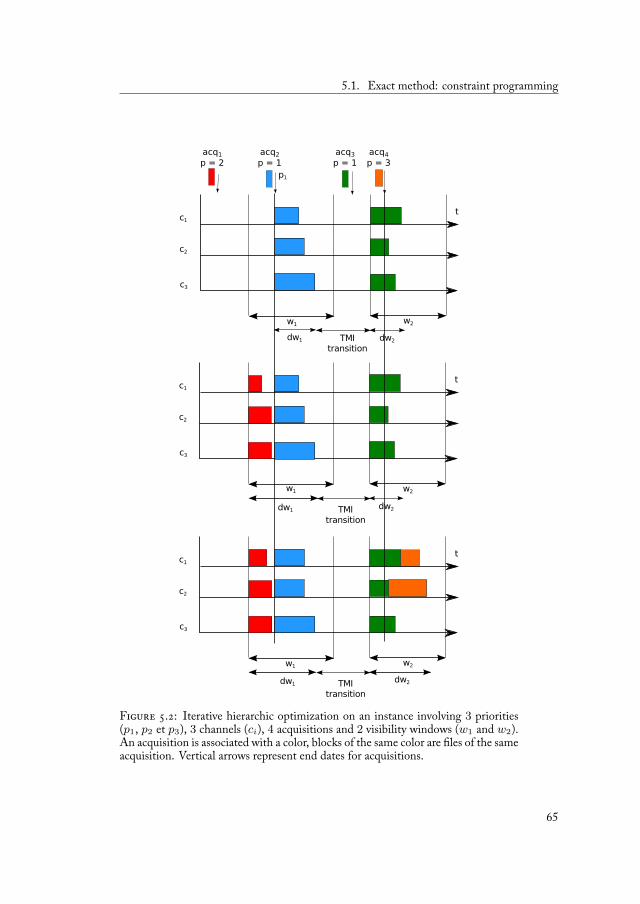
5.1. Exact method: constraint programming
F . : Iterative hierarchic optimization on an instance involving 3 priorities(p1, p2 et p3), 3 channels (ci), 4 acquisitions and 2 visibility windows (w1 and w2).An acquisition is associated with a color, blocks of the same color are les of the sameacquisition. Vertical arrows represent end dates for acquisitions.
65
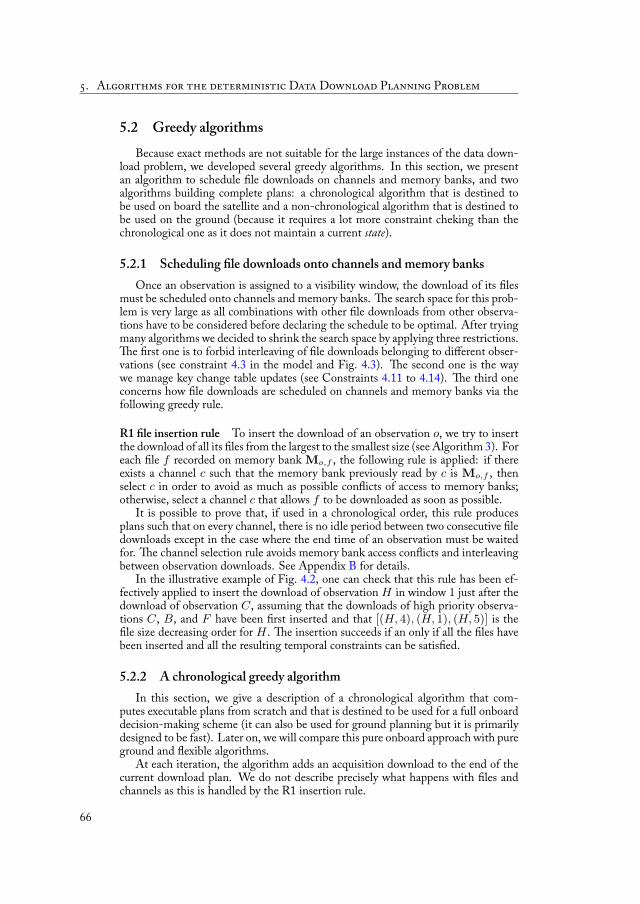
. A D D P P
5.2 Greedy algorithmsBecause exact methods are not suitable for the large instances of the data down-
load problem, we developed several greedy algorithms. In this section, we presentan algorithm to schedule le downloads on channels and memory banks, and twoalgorithms building complete plans: a chronological algorithm that is destined tobe used on board the satellite and a non-chronological algorithm that is destined tobe used on the ground (because it requires a lot more constraint cheking than thechronological one as it does not maintain a current state).
5.2.1 Scheduling le downloads onto channels and memory banksOnce an observation is assigned to a visibility window, the download of its les
must be scheduled onto channels and memory banks. e search space for this prob-lem is very large as all combinations with other le downloads from other observa-tions have to be considered before declaring the schedule to be optimal. After tryingmany algorithms we decided to shrink the search space by applying three restrictions.
e rst one is to forbid interleaving of le downloads belonging to different obser-vations (see constraint 4.3 in the model and Fig. 4.3). e second one is the waywe manage key change table updates (see Constraints 4.11 to 4.14). e third oneconcerns how le downloads are scheduled on channels and memory banks via thefollowing greedy rule.
R1 le insertion rule To insert the download of an observation o, we try to insertthe download of all its les from the largest to the smallest size (see Algorithm 3). Foreach le f recorded on memory bank Mo,f , the following rule is applied: if thereexists a channel c such that the memory bank previously read by c is Mo,f , thenselect c in order to avoid as much as possible con icts of access to memory banks;otherwise, select a channel c that allows f to be downloaded as soon as possible.
It is possible to prove that, if used in a chronological order, this rule producesplans such that on every channel, there is no idle period between two consecutive ledownloads except in the case where the end time of an observation must be waitedfor. e channel selection rule avoids memory bank access con icts and interleavingbetween observation downloads. See Appendix B for details.
In the illustrative example of Fig. 4.2, one can check that this rule has been ef-fectively applied to insert the download of observation H in window 1 just after thedownload of observation C, assuming that the downloads of high priority observa-tions C, B, and F have been rst inserted and that [(H, 4), (H, 1), (H, 5)] is thele size decreasing order for H . e insertion succeeds if an only if all the les have
been inserted and all the resulting temporal constraints can be satis ed.
5.2.2 A chronological greedy algorithmIn this section, we give a description of a chronological algorithm that com-
putes executable plans from scratch and that is destined to be used for a full onboarddecision-making scheme (it can also be used for ground planning but it is primarilydesigned to be fast). Later on, we will compare this pure onboard approach with pureground and exible algorithms.
At each iteration, the algorithm adds an acquisition download to the end of thecurrent download plan. We do not describe precisely what happens with les andchannels as this is handled by the R1 insertion rule.
66

5.2. Greedy algorithms
u1
u2
u3
u4
u5
w1
w3
w4
w2
u1
u2
u3
u4
u5
w1
w3
w4
w2
iteration 0 iteration 1
u1
u2
u3
u4
u5
w1
w3
w4
w2
u1
u2
u3
u4
u5
w1
w3
w4
w2
iteration 2 iteration 3
u1
u2
u3
u4
u5
w1
w3
w4
w2
u1
u2
u3
u4
u5
w1
w3
w4
w2
iteration 4 iteration 5
u1
u2
u3
u4
u5
w1
w3
w4
w2
u1
u2
u3
u4
u5
w1
w3
w4
w2
iteration 6 iteration 7
F . : Iterations of the chronological greedy algorithm, macroscopic viewwithout les and channels.
67
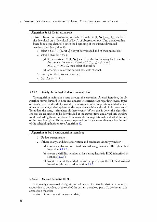
. A D D P P
Algorithm 3: R1 le insertion rule1 Data : observation o to insert; for each channel c ∈ J1, NcK, (oc, fc), the last
le download on c (download of le fc of observation oc). If no download hasbeen done using channel c since the beginning of the current downloadwindow, then (oc, fc) = ∅;
1. select a le f ∈ J1, Nf oK not yet downloaded and of maximum size;2. select a channel c for f :
(a) if there exists c ∈ J1, NcK such that the last memory bank read by c isthe same as the memory bank of f ((oc, fc) = ∅ andMoc,fc = Mo,f ), then select channel c;
(b) otherwise, select the earliest available channel;3. insert f on the chosen channel c;4. (oc, fc)← (o, f).
5.2.2.1 Greedy chronological algorithm main loope algorithm maintains a state through the execution. At each iteration, the al-
gorithm moves forward in time and updates its current state regarding several typesof events : start and end of a visibility window, end of an acquisition, end of an an-tenna movement, end of updates of the key change tables and end of le downloads.To update the state, it simulates all these events. When this is done, the algorithmchooses an acquisition to be downloaded at the current time and a visibility windowfor downloading this acquisition. It then inserts the acquisition download at the endof the download plan. is scheme is repeated until the current time reaches the endof the scheduling horizon (see Algorithm 4).
Algorithm 4: Full board algorithm main loop1. Update current state;2. if there is any candidate observation and candidate visibility window :
a) choose an observation o to download using heuristic HD1 (describedin section 5.2.2.2);
b) choose a visibility window w for o using heuristic HD2 (described insection 5.2.2.3);
c) insert o in w at the end of the current plan using the R1 le downloadinsertion rule described in section 5.2.1.
5.2.2.2 Decision heuristic HD1e greedy chronological algorithm makes use of a rst heuristic to choose an
acquisition to download at the end of the current download plan. To be chosen, thisacquisition must be:
– stored in memory at the current date;
68
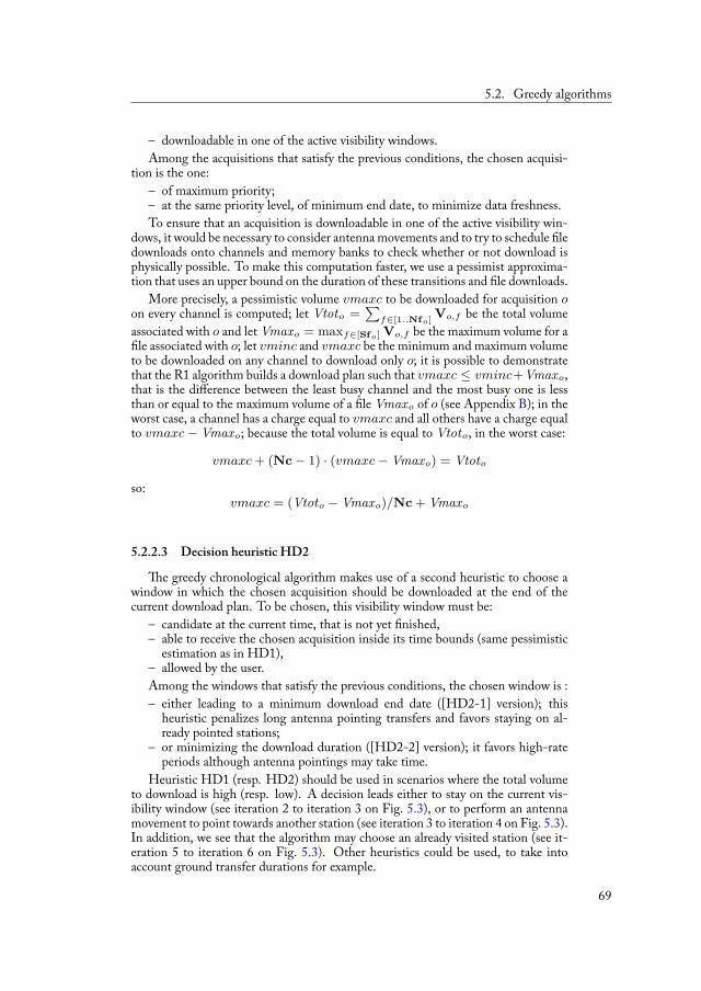
5.2. Greedy algorithms
– downloadable in one of the active visibility windows.Among the acquisitions that satisfy the previous conditions, the chosen acquisi-
tion is the one:– of maximum priority;– at the same priority level, of minimum end date, to minimize data freshness.To ensure that an acquisition is downloadable in one of the active visibility win-
dows, it would be necessary to consider antenna movements and to try to schedule ledownloads onto channels and memory banks to check whether or not download isphysically possible. To make this computation faster, we use a pessimist approxima-tion that uses an upper bound on the duration of these transitions and le downloads.
More precisely, a pessimistic volume vmaxc to be downloaded for acquisition oon every channel is computed; let Vtoto =
∑f∈[1..Nfo] Vo,f be the total volume
associated with o and let Vmaxo = maxf∈[Sfo] Vo,f be the maximum volume for ale associated with o; let vminc and vmaxc be the minimum and maximum volume
to be downloaded on any channel to download only o; it is possible to demonstratethat the R1 algorithm builds a download plan such that vmaxc ≤ vminc+Vmaxo,that is the difference between the least busy channel and the most busy one is lessthan or equal to the maximum volume of a le Vmaxo of o (see Appendix B); in theworst case, a channel has a charge equal to vmaxc and all others have a charge equalto vmaxc−Vmaxo; because the total volume is equal to Vtoto, in the worst case:
vmaxc + (Nc− 1) · (vmaxc−Vmaxo) = Vtoto
so:vmaxc = (Vtoto −Vmaxo)/Nc + Vmaxo
5.2.2.3 Decision heuristic HD2
e greedy chronological algorithm makes use of a second heuristic to choose awindow in which the chosen acquisition should be downloaded at the end of thecurrent download plan. To be chosen, this visibility window must be:
– candidate at the current time, that is not yet nished,– able to receive the chosen acquisition inside its time bounds (same pessimistic
estimation as in HD1),– allowed by the user.Among the windows that satisfy the previous conditions, the chosen window is :– either leading to a minimum download end date ([HD2-1] version); this
heuristic penalizes long antenna pointing transfers and favors staying on al-ready pointed stations;
– or minimizing the download duration ([HD2-2] version); it favors high-rateperiods although antenna pointings may take time.
Heuristic HD1 (resp. HD2) should be used in scenarios where the total volumeto download is high (resp. low). A decision leads either to stay on the current vis-ibility window (see iteration 2 to iteration 3 on Fig. 5.3), or to perform an antennamovement to point towards another station (see iteration 3 to iteration 4 on Fig. 5.3).In addition, we see that the algorithm may choose an already visited station (see it-eration 5 to iteration 6 on Fig. 5.3). Other heuristics could be used, to take intoaccount ground transfer durations for example.
69

. A D D P P
5.2.3 A non-chronological greedy algorithmis algorithm, as the chronological algorithm, builds a download schedule from
scratch. It is primarily designed to be used on the ground as it is non-chronologicaland then requires constraint propagation at each iteration.
e principle of the non-chronological greedy algorithm is very basic. It insertsacquisition downloads one after each other in the plan following an insertion order A(see Algorithm 5) given as an input (ordering observations by priorities and then byweights is a straightforward method to produce such an insertion order). e algo-rithm is said to be non-chronological because an observation that is considered lateraccording to the speci ed order may be nally downloaded earlier in the resultingdownload plan [Pralet et al., 2014b].
Algorithm 5: Non-chronological greedy algorithm1 Data : O = [o1, ..., on] the ordered set of candidate acquisitions over the
planning horizon1. Init P , an empty plan2. For i : 1→ n
a) Choose a visibility window wi ∈ J1, NwK and a position ki ∈ J1, nKin the sequence of acquisition downloads for oi using heuristic H1;
b) Insert (oi, wi) at position ki in the sequence of downloadsc) Insert all les of oi using rule R1;d) Check constraints;e) If constraint violation, undo changes and go to (a) when other (wi, ki)
pairs can be selected.
e algorithm starts from an empty schedule and considers all the observationsin the speci ed order. For each of them, it tries to insert its download in the cur-rent download schedule. To insert the download of an observation o, the algorithmexplores all the pairs made of a download window w and of a position k in the se-quence of downloads already scheduled. Pairs are explored chronologically from theearliest to the latest in order to minimize information age. After each insertion, allthe non-temporal constraints are checked and all the temporal constraints are prop-agated in the current TSTN (see Sect. 5.2.3.2 for more details). If any constraint isviolated, another pair window/position is selected for o until all the possible pairs areexhausted. If all of them have been exhausted without any success, o is rejected.
Fig. 5.4 shows the rst iterations of the non-chronological greedy algorithm.ere are ve users (u1 to u5). Each iteration adds a new observation download
in the plan, not necessarily at the end. See for example between iteration 3 and iter-ation 4, where an acquisition associated with user u2 is added before other downloadsalready in the plan.
5.2.3.1 H1 decision heuristic
e H1 decision heuristic chooses an allowed visibility window w and a positionp for o in the current download sequence dSeq = [o1, . . . , on]. ere are two
70
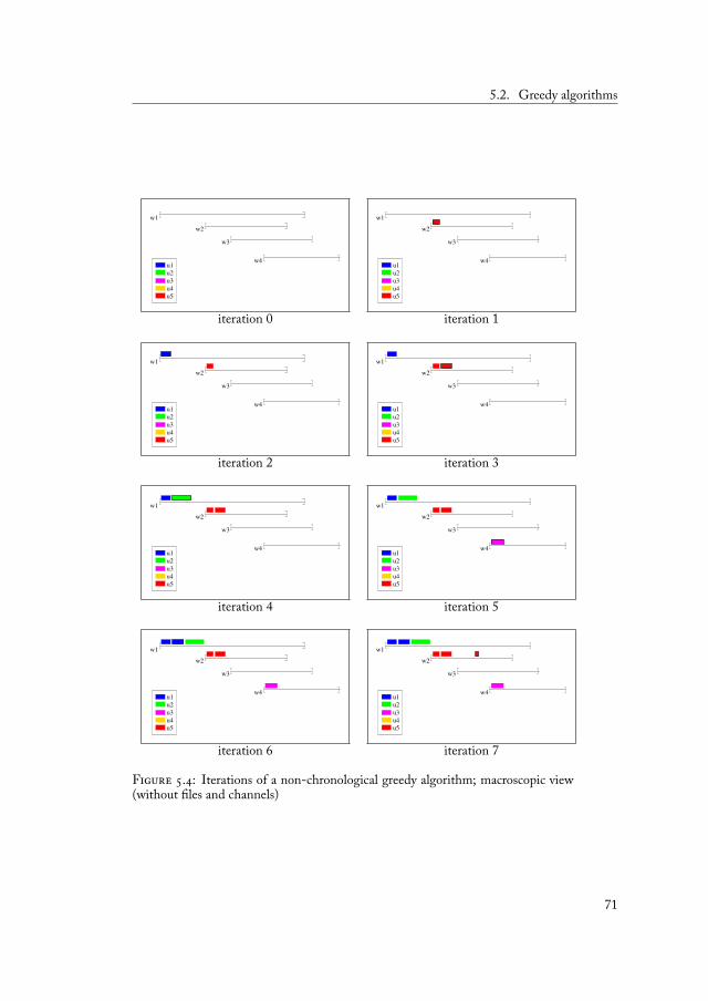
5.2. Greedy algorithms
u1
u2
u3
u4
u5
w1
w3
w4
w2
u1
u2
u3
u4
u5
w1
w3
w4
w2
iteration 0 iteration 1
u1
u2
u3
u4
u5
w1
w3
w4
w2
u1
u2
u3
u4
u5
w1
w3
w4
w2
iteration 2 iteration 3
u1
u2
u3
u4
u5
w1
w3
w4
w2
u1
u2
u3
u4
u5
w1
w3
w4
w2
iteration 4 iteration 5
u1
u2
u3
u4
u5
w1
w3
w4
w2
u1
u2
u3
u4
u5
w1
w3
w4
w2
iteration 6 iteration 7
F . : Iterations of a non-chronological greedy algorithm; macroscopic view(without les and channels)
71

. A D D P P
versions for this heuristic. In the following paragraph, let Vtoto be the total volumeassociated with observation o, with Vtoto =
∑f∈[Sfo] Vo,f .
De nition: Idle period Let dSeq = [o1, . . . , on] be the sequence of observationdownloads. It is said that there is an idle period between two downloads oi−1 and oi
in the sequence if and only if the download end date sdooi−1 of the les of oi−1 isnot constraining the download start date of the les of oi. More formally, there is anidle period before the observation download oi if and only if the smallest downloadstart date of a le of oi is equal to the visibility window start date which contains oi
(date Swdwoi) or to the end of the observation oi (date Eooi ). is de nition is
valid even if oi is the rst observation download of the plan. Note that observationsending during the planning horizon may induce idle periods.
[H1-1] version e rst version of the H1 heuristic, H1-1, aims at optimizing datafreshness. e heuristic chooses rst an allowed visibility window w such that theestimated delivery date to the requesting user is minimized for the selected observa-tion.
To compute this estimated delivery date, we maintain for each visibility windoww and each user u allowing downloads onto w, the volume Vgndw,u of data down-loaded onto w and aimed at u in the schedule. ese volumes are initialized to 0.
An optimistic estimation eo,w of the delivery date for the observation o to bedownloaded onto w is given by:
eo,w = max(Sww, Eoo)+DuDl(Vtoto/Nc, w, max(Sww, Eoo))+(Vgndw,Uo
+ Vtoto)/GtrStw,Uo
or, in other words, it is the sum of:– an optimistic estimation of the earliest download start date of o
(max(Sww, Eoo));– an optimistic estimation of the required duration for download-
ing o with an equitable repartition of the volume over the channels(DuDl(Vtoto/Nc, w, max(Sww, Eoo)), with DuDl(v, w, t) whichreturns the required duration to download a volume v onto window w whenstarting at time t;
– a realistic estimation of the required duration for transmitting the acquisitionreceived by w; the estimation uses the ground transfer rate between the groundreception station Stw and the production center associated to the user request-ing o ((Vgndw,Uo
+ Vtoto)/GtrStw,Uo ); it also implicitly models networkcongestion by considering that o is transmitted last.e H1-1 heuristic selects a visibility window w, allowed for user Uo, such that
the estimation eo,w is minimized. When an acquisition download o is actually in-serted into w, the volume of data downloaded onto w is incremented as:
Vgndw,Uo← Vgndw,Uo
+ Vtoto
Once w has been selected, an insertion position p is to be chosen. To nd a goodposition, the heuristic chronologically traverses the download sequence dSeq =[o1, . . . , on]. At each step, if oi is the next acquisition to be downloaded:
72
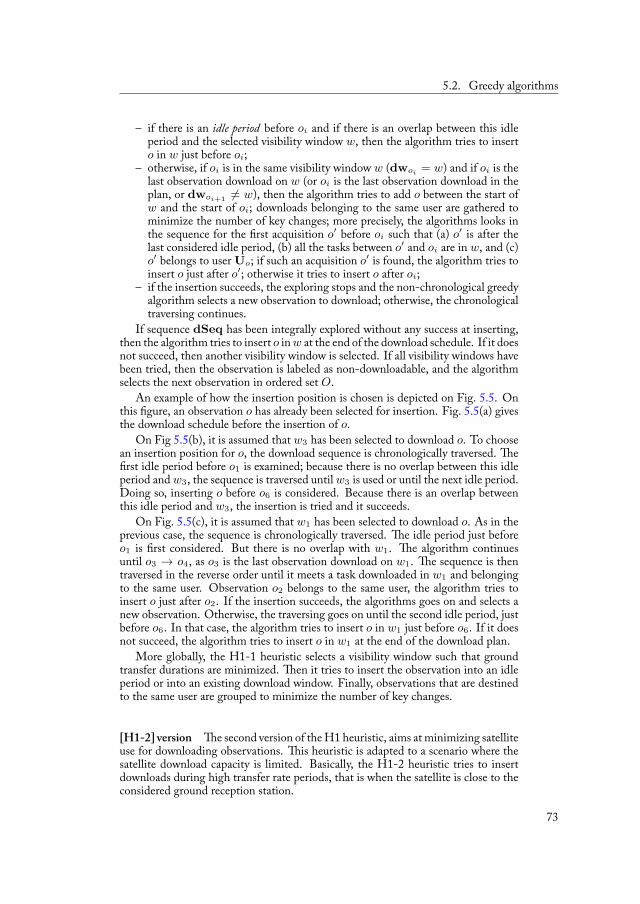
5.2. Greedy algorithms
– if there is an idle period before oi and if there is an overlap between this idleperiod and the selected visibility window w, then the algorithm tries to inserto in w just before oi;
– otherwise, if oi is in the same visibility window w (dwoi = w) and if oi is thelast observation download on w (or oi is the last observation download in theplan, or dwoi+1 = w), then the algorithm tries to add o between the start ofw and the start of oi; downloads belonging to the same user are gathered tominimize the number of key changes; more precisely, the algorithms looks inthe sequence for the rst acquisition o′ before oi such that (a) o′ is after thelast considered idle period, (b) all the tasks between o′ and oi are in w, and (c)o′ belongs to user Uo; if such an acquisition o′ is found, the algorithm tries toinsert o just after o′; otherwise it tries to insert o after oi;
– if the insertion succeeds, the exploring stops and the non-chronological greedyalgorithm selects a new observation to download; otherwise, the chronologicaltraversing continues.
If sequence dSeq has been integrally explored without any success at inserting,then the algorithm tries to insert o in w at the end of the download schedule. If it doesnot succeed, then another visibility window is selected. If all visibility windows havebeen tried, then the observation is labeled as non-downloadable, and the algorithmselects the next observation in ordered set O.
An example of how the insertion position is chosen is depicted on Fig. 5.5. Onthis gure, an observation o has already been selected for insertion. Fig. 5.5(a) givesthe download schedule before the insertion of o.
On Fig 5.5(b), it is assumed that w3 has been selected to download o. To choosean insertion position for o, the download sequence is chronologically traversed. erst idle period before o1 is examined; because there is no overlap between this idle
period and w3, the sequence is traversed until w3 is used or until the next idle period.Doing so, inserting o before o6 is considered. Because there is an overlap betweenthis idle period and w3, the insertion is tried and it succeeds.
On Fig. 5.5(c), it is assumed that w1 has been selected to download o. As in theprevious case, the sequence is chronologically traversed. e idle period just beforeo1 is rst considered. But there is no overlap with w1. e algorithm continuesuntil o3 → o4, as o3 is the last observation download on w1. e sequence is thentraversed in the reverse order until it meets a task downloaded in w1 and belongingto the same user. Observation o2 belongs to the same user, the algorithm tries toinsert o just after o2. If the insertion succeeds, the algorithms goes on and selects anew observation. Otherwise, the traversing goes on until the second idle period, justbefore o6. In that case, the algorithm tries to insert o in w1 just before o6. If it doesnot succeed, the algorithm tries to insert o in w1 at the end of the download plan.
More globally, the H1-1 heuristic selects a visibility window such that groundtransfer durations are minimized. en it tries to insert the observation into an idleperiod or into an existing download window. Finally, observations that are destinedto the same user are grouped to minimize the number of key changes.
[H1-2] version e second version of the H1 heuristic, aims at minimizing satelliteuse for downloading observations. is heuristic is adapted to a scenario where thesatellite download capacity is limited. Basically, the H1-2 heuristic tries to insertdownloads during high transfer rate periods, that is when the satellite is close to theconsidered ground reception station.
73
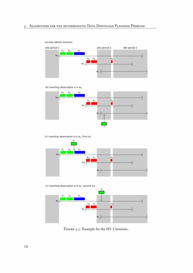
. A D D P P
F . : Example for the H1-1 heuristic.
74

5.2. Greedy algorithms
Compared to the H1-1 heuristic which chooses rst a window and then a posi-tion in the download sequence, the H1-2 heuristic chooses simultaneously a visibilitywindow w and a position p. To make this choice (w, p), H1-2 chronologically tra-verses idle periods.
For each idle period P , the algorithm tries to insert o into P . More precisely, leto′ denote the next observation just after P , if it exists. en,
– the algorithm evaluates the insertion of o just before o′ for all allowed visibilitywindows w that overlap P ; this evaluation uses the metric duVido, an estimateof the download duration of o; the visibility window w which minimizes duVidis kept, to consider rst high transfer rate periods; let duVid∗ be the durationgiven by this best option; in what follows, any better option for inserting omust not decrease the idle period by a duration higher than duVid∗ + 1 (1 isa penalty for depointing);
– the algorithm evaluates the insertion of o in download windows that are beforethe current idle period; to do this, the sequence of downloads is traversed inreverse order from o′; when there is a task oi downloaded in a different visibilitywindow w than the one used for oi+1, the algorithm assess whether insertingo into w after oi is better than the best option found so far; if it is the case, thecurrent insertion position is kept;
– when the previous analysis has been done, the algorithm tries to insert theobservation at the best position, and observations that are destined to the sameuser are grouped to minimize the number of key changes.
If an insertion has failed, the next idle period is analyzed. As soon as an insertionsucceeds, the algorithm selects a new observation to download.
Fig. 5.6 shows an example of insertion positions considered by H1-2. e con-sidered idle period is the one before o6. e H1-2 heuristic tries to ll the idle periodand to minimize satellite use.
F . : Example for the H1-2 heuristic.
5.2.3.2 Constraint checkingAfter each observation download insertion, the resulting download schedule can
be checked with regard to all the temporal constraints. As already said in Sect. 4.2.5,the resulting temporal problem forms a TSTN. e InCELL library [Pralet and
75

. A D D P P
Verfaillie, 2013a] is used to determine whether or not the TSTN is consistent and, incase of consistency, to compute the earliest and latest times of each temporal variable.
InCELL is a generic constraint-based evaluation library developed at Onerawhich allows constraint-based models to be formulated, non temporal constraintsand criteria to be evaluated, and temporal (time-dependent or not) constraints to bepropagated. Its has been built from the ideas of constraint-based local search [Hen-tenryck and Michel, 2005] and around the notion of invariant and of DAG (directedacyclic graph) of invariants. Any constraint optimization problem is modeled as aDAG of invariants with decision variables at the roots of the DAG and constraintsand criterion at the leaves. DAG modeling allows any assignment of the decisionvariables to be evaluated (checking of the constraints and evaluation of the criterion).In the context of a greedy or local search, it allows any new (neighbor) assignment tobe very quickly reevaluated thanks to an incremental reevaluation mechanism. isallows each local move to be quickly performed and a huge number of local movesto be performed in a limited amount of time. Moreover, InCELL includes sev-eral modeling and solving functionalities speci cally dedicated to the managementof (oversubscribed) scheduling problems: for example, existence of global (T)STNinvariants in charge of the propagation of temporal constraints.
When a download schedule has been built, with all its constraints checked, anearliest schedule can be produced (see the example of Fig. 4.2). However temporalvariables can remain unassigned and a partial order schedule de ned by a precedencegraph can also be produced to allow a exible schedule execution (see Sect. 6.4).
5.3 Metaheuristic: Squeaky Wheel Optimizatione non-chronological algorithm takes an insertion order as input. is order can
be determined either with a heuristic once for all or updated during search. One issueis that this insertion order has a great in uence on the result and the heuristic canbe bad. at is why an algorithm designed to avoid such a situation has been used:Squeaky Wheel Optimization, which is a general method for solving combinatorialproblems [Joslin and Clements, 1999]. Basically, there are three components in anSWO algorithm :
– a builder, which consists in a greedy algorithm without backtrack; an orderedlist of elements is used by this algorithm in order to allocate resources in anordered manner;
– the grader; after a valid plan has been produced, the grader analyzes the planand blames elements which deteriorate the most the solution; it generates agrade for each element: the higher the grade, the higher the deterioration;
– the prioritizer, which changes the order of elements in the list according totheir grades; the more the grade of an element is high the more this element ismoved forward in the list; the idea is to allocate resources earlier for elementswhich have a high grade because they deteriorate the most the solution.
SWO is primarily moving into the priority space. A small number of changes intothe priority space may be a large step into the solution space. is characteristic is im-portant for searching solutions for scheduling problem as this class of problems oftenhave large plateaus in terms of criterion [Barbulescu et al., 2006]. Algorithm 6 showshow we build upon the non-chronological greedy algorithm presented in Sec. 5.2.3to obtain an SWO search scheme.
For the rst greedy search, observations are ordered in O′ from the highest to thelowest priority level and, at the same priority level, from the biggest to the lowest
76

5.3. Metaheuristic: Squeaky Wheel Optimization
Algorithm 6: Squeaky Wheel Optimization1 Data : O, the set of candidate observations over the planning horizon;
1. Init O′, an ordering of O;2. i← 0;3. While time is available :
a) i← i + 1;b) From O′, build a plan Pi using a greedy algorithm (see Algorithm 5
and Algorithm 4);c) Save Pi;d) Analyze weaknesses of Pi;e) Modify O′ by moving forward observations whose freshness is low in
Pi;4. Select P in P1, ..., Pi such that the optimization criterion is maximum.
weight, in order to favor high-priority acquisitions. In our case, the grade associatedwith each acquisition o for a plan Pi depends on the freshness of o in Pi. Aftereach greedy search producing a plan Pi, the insertion order O′, between acquisitionsof the same priority, is updated by moving sequentially forward in O′ acquisitionswhose freshness is lower than the mean freshness. is move is proportional to thedifference between both freshnesses.
To be more concrete, let fro be the freshness of o in a plan P . Let f be the meanfreshness over all downloaded acquisitions. Let fW and fB be respectively the worstand best freshness in the plan, and let be ip the index of o in the sub-sequence ofpriority p in O′. If fro < f , acquisition o is moved forward in O′ and its new indexi′p in the sub-sequence of priority p is :
i′p =
⌊
ip −f − fro
fW − fB× ip
⌋if fro < f
ip otherwise(5.2)
is process is repeated as shown in Algorithm 6. e best plan over all theruns according to the optimization criterion (see Sect 4.2.4.2) is nally selected. Anexample can be seen on Fig. 5.7. is example aims at showing that the insertionorder has a great important with respect to the solution quality. In this example, thereare four observations o1, o2, o3, o4 to be downloaded. Each observation oi mayonly be downloaded in one visibility window wi. At each iteration, a chronologicalalgorithm takes observations from the ordered list, puts them in the plan and buildsa complete plan. In the rst iteration, o1 and o2 are downloaded as soon as possiblewhich results in preventing o3 and o4 from being downloaded. In iteration 2, theorder is updated with respect to the absence of o3 and o4 in the schedule, movingthem forward in the insertion order. In iteration 3, o4 is inserted rst which allowsto download it during its only possible window.
e SWO scheme may be used with the non-chronological algorithm and stayvery useful as the order of insertion is critical in this algorithm with regard the ex-ploration of the solution space.
77
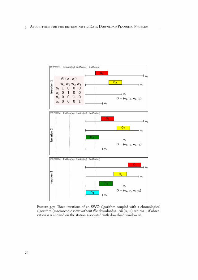
. A D D P P
F . : ree iterations of an SWO algorithm coupled with a chronologicalalgorithm (macroscopic view without le downloads). All(o, w) returns 1 if obser-vation o is allowed on the station associated with download window w.
78
5.4. Analysis
5.4 AnalysisEach algorithm has its advantages and drawbacks. e greedy chronological al-
gorithm is faster and has a smaller memory consumption. It is because it only main-tains a current state rather than maintaining a model of the problem over the wholeplanning horizon. On the negative side, building efficient heuristics for this type ofalgorithm is not always easy and the algorithm often ends up to be myopic.
e non-chronological greedy algorithm is slower and has a greater memory con-sumption but it is built upon a formal model which is easily updatable. In addition,it is less myopic that the chronological version because it is reasoning over the wholeplanning horizon. Typically, it produces plans with less go-and-back between groundstations and less key changes, thanks to the heuristic that groups downloads associ-ated with the same user. By contrast with the chronological version, when insertinga download before existing downloads, it must often propagate and check the con-straints through the whole horizon, which is a costly operation. Another drawbackis the high dependence on the input ordered list.
at is why a Squeaky Wheel Optimization scheme has been developed upon thenon-chronological algorithm. By updating the list after each iteration, it explores thesolution space efficiently. However, it still depends on the internal heuristics of thealgorithm. A way to deal with this would be to introduce stochastic parameters intothe heuristics so that there is a probability to make another decision given the sameinitial state.
All these algorithms are used in the next chapter to design full decision-makingschemes.
79

Flexible Scheduling for the Data Download Problem 6
6.1 Overview of the decision-making organization . . . . . . . . 796.1.1 Overview of the pure ground approach . . . . . . . 796.1.2 Overview of the pure onboard approach . . . . . . . 816.1.3 Overview of the ground-onboard mixed approach . . 83
6.2 Scheduling on the ground . . . . . . . . . . . . . . . . . . . 846.3 Adapting data download schedules on board . . . . . . . . . 85
6.3.1 Preparing download schedule adaptation on the ground 866.3.2 Performing download schedule adaptation on board . 88
6.4 Executing on-board . . . . . . . . . . . . . . . . . . . . . . 946.4.1 Temporal exibility at execution . . . . . . . . . . . 946.4.2 Building a exible plan from a complete plan . . . . 946.4.3 Execution . . . . . . . . . . . . . . . . . . . . . . 97
6.5 Experiments . . . . . . . . . . . . . . . . . . . . . . . . . 986.5.1 Approaches to be compared . . . . . . . . . . . . . 986.5.2 Scenarios . . . . . . . . . . . . . . . . . . . . . . 996.5.3 Evaluation criteria . . . . . . . . . . . . . . . . . . 996.5.4 Result analysis . . . . . . . . . . . . . . . . . . . . 100
6.6 Discussion . . . . . . . . . . . . . . . . . . . . . . . . . . 1046.6.1 Decisional exibility . . . . . . . . . . . . . . . . . 1046.6.2 Missing evaluation and future works . . . . . . . . . 104
In the previous chapters, we presented the data download problem and algorithmsto solve its deterministic version. In this chapter, we present a exible approach toshare decision-making on data downloads between ground and board. For that wedescribe the decision-making chain organization from the ground planning to theonboard execution for several approaches: pure ground scheduling, pure onboardscheduling, and the contribution of this chapter, exible scheduling.
6.1 Overview of the decision-making organizationIn this section, we show how decision-making about observations and downloads
can be organized in each of the three approaches we compare.
6.1.1 Overview of the pure ground approachFig. 6.1 shows the overall organization of decision-making in the pure ground
approach, where all the decisions are made on the ground in the mission center. Suchan approach is used to manage the currently operational Earth-observing Pleiadessatellites.
81
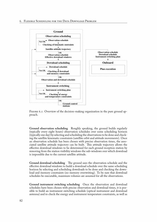
. F S D D P
Observation schedule
Observation scheduling
Checking of kinematic onstraints
Satellite attitude trajectory
OK
OK
Not OK
Not OK
Instrument switching
OK
and temperature constraints
Instrument switching plan
Instrument switching plan
Checking of energy
Observation scheduleDownload schedule
Plan execution
Ground
Observation scheduleEffective download windows
Download scheduling
Observation and download schedule
Checking of download
Download schedule
Not OK
and memory constraints
stationsGround control
Onboard
F . : Overview of the decision-making organization in the pure ground ap-proach.
Ground observation scheduling Roughly speaking, the ground builds regularly(typically every eight hours) observation schedules over some scheduling horizon(typically one day) by selecting and scheduling the observations to be done and check-ing the satellite kinematic constraints (satellite orbit and attitude movements). Oncean observation schedule has been chosen with precise observation times, the asso-ciated satellite attitude trajectory can be built. is attitude trajectory allows theeffective download windows to be determined for each ground reception station byremoving from the station visibility windows the sub-windows over which downloadis impossible due to the current satellite attitude.
Ground download scheduling e ground uses the observation schedule and theeffective download windows to build a download schedule over the same schedulinghorizon by selecting and scheduling downloads to be done and checking the down-load and memory constraints (no memory overwriting). To be sure that downloadschedules be executable, maximum volumes are assumed for all the observations.
Ground instrument switching scheduling Once the observation and downloadschedules have been chosen with precise observation and download times, it is pos-sible to build an instrument switching schedule (optical instrument and downloadantenna) and to check the energy and instrument temperature constraints, as well as
82

6.1. Overview of the decision-making organization
the instrument limitations in terms of On duration and number of On/Off over thescheduling horizon.
Onboard schedule execution Once all these schedules have been built on theground, they can be sent to the satellite using any ground control station visibilitywindow and then executed as they are, without any change.
e rst justi cation for this decision-making organization is that one needs toknow the observation schedule to build the satellite attitude trajectory, the effectivedownload windows, and then the download schedule, and that one needs to know theobservation and download schedules to build the instrument switching schedule. esecond justi cation is that is has been observed on the currently operational Earth-observing Pleiades satellites that the limitations of the system in terms of observationcapacity come in a decreasing order of impact from (1) the kinematic satellite attitudeconstraints, (2) the download constraints, (3) the energy constraints, (4) the instru-ment temperature constraints, and (5) the mass memory constraints. Checking rstthe most limiting constraints is known as a good practice.
6.1.2 Overview of the pure onboard approachFig. 6.2 shows the overall organization of decision-making in the pure onboard
approach, where all the decisions about downloads are made on board. Such anapproach has been explored in [Pralet et al., 2014c].
Observation scheduling
Observation schedule
Satellite attitude trajectory
Checking of kinematic onstraints
Not OK
OK
Ground
Not OK
Instrument switching
Instrument switching plan
and temperature constraintsChecking of energy
OK
Ground controlstations
Observation schedule
Observation scheduleEffective download windowsInstrument switching plan
Download scheduling
Download schedule
download constraintsChecking ofNot OK
OK
Observation execution
Checking ofmemory constraints
Download execution
Execution of theprecedence graph
Download precedence graph
Onboard
F . : Overview of the decision-making organization in the pure onboard ap-proach.
Ground observation scheduling Observation scheduling is performed on theground in the mission center exactly as it is in the pure ground approach.
Ground instrument switching scheduling Because we do not know on the groundthe downloads that will be decided on board, we make the pessimistic assumptionthat all the effective download windows will be entirely used for data downloading.On this basis, it is possible to build an instrument switching schedule and to check the
83

. F S D D P
energy and instrument temperature constraints, as well as the instrument limitationsin terms of On duration and number of On/Off.
Onboard download scheduling e observation schedule and the effective down-load windows can then be sent to the satellite using any ground control station vis-ibility window and used for download scheduling. On board, because informationabout the actual volumes to be downloaded arrives as observations nish, downloadscheduling is performed just before any group of overlapping download windows (atthe latest time to take advantage of the maximum information), with this group ofwindows as scheduling horizon. Two download windows are considered as over-lapping if and only if they effectively overlap or there is not enough time betweenthe end of the rst and the beginning of the second to decompose the downloadscheduling problem into two subproblems. Exact volumes are considered for all theobservations that are nished at the scheduling time and maximum volumes for thosethat will nish between the scheduling time and the end of the scheduling horizonin order to guarantee that download schedules be executable.
Onboard observation and instrument switching execution Observations are per-formed and instruments are switched as speci ed by the ground observation andinstrument switching schedules. However, because the memory constraint cannotbe checked on the ground (downloads not decided yet), a simple mechanism is usedon board when executing observations in order to avoid any memory overwriting:if performing an observation o may lead to a memory overwriting, either o is notperformed, or lower priority data is removed from memory to free space.
Onboard download execution Downloads are performed as speci ed by the suc-cessive download schedules, over the successive groups of overlapping download win-dows. However, to take into account the remaining uncertainty about the volumes ofdata produced by the observations that will nish between the scheduling time andthe end of the scheduling horizon, the download schedules sent for execution arenot xed, but remain temporally exible. Concretely, they have the form of a prece-dence DAG (Directed Acyclic Graph) where each node is executed as soon as all itspredecessor nodes have been executed. is allows to take advantage of downloadswhose duration is strictly smaller than the maximum duration that has been con-sidered when scheduling and thus to start downloads earlier than in the pessimisticdownload schedule.
Keeping observation scheduling on the ground is justi ed by the fact that obser-vation scheduling calls for time consuming computations of satellite attitude move-ments: movements to move from any observation to the following and precise move-ments to perform any observation with the required quality level. ese movementsare far more complex with agile satellites (movements of the whole satellite) thanwith previous generation non agile satellites, such as the rst Spot satellites (move-ments of a mobile mirror). Engineers consider that the current technology does notallow these movements to be efficiently computed on board. On the contrary, mov-ing download scheduling on board is justi ed by the fact that download schedulingis far less time consuming than observation scheduling is. is organization is alsojusti ed by the fact that uncertainty about volumes of data directly impacts downloadscheduling, but only indirectly observation scheduling.
84

6.1. Overview of the decision-making organization
6.1.3 Overview of the ground-onboard mixed approachFig. 6.3 shows the overall organization of decision-making in the ground-
onboard mixed approach, where the decisions about downloads are shared betweenground and onboard.
Observation execution
Checking ofmemory constraints
Observation schedule
Observation scheduling
Checking of kinematic onstraints
Satellite attitude trajectory
OK
OK
Not OK
Not OK
Instrument switching
OK
and temperature constraints
Instrument switching plan
Ground
Checking of energy
Observation scheduleEffective download windows
Download scheduling
Observation and download schedule
Checking of download
Download schedule
Not OK
and memory constraints
stationsGround control
Download execution
OK
precedence graphExecution of the
adaptation
Download precedence graph
Download schedule
Download schedule
download constraintsChecking of
Not OK
and commitments
Commitments
Instrument switching plan
Effective download windowsDownload schedule
Onboard
Observation schedule
Maximum resource consumption levels
F . : Overview of the decision-making organization in the mixed ground-onboard approach.
With each observation, is associated a priority level de ned by an integer between1 and Np, with 1 the highest priority level and Np the lowest. In the sequel of thischapter, we refer to as high priority observations all the observations of priority level1 and as low priority observations all the others, of priority level greater than or equalto 2.
Ground observation scheduling Observation scheduling is performed on theground in the mission center exactly as it is in the previous two approaches.
Ground download scheduling e ground uses the acquisition schedule and theeffective download windows to build a download schedule over the same schedulinghorizon by selecting and scheduling downloads to be done and checking the down-load and memory constraints as it is done in the pure ground approach. e onlydifference is that maximum volumes are assumed only for the high priority obser-vations in order to guarantee that these observations be anyway downloaded. Forthe low priority observations, for which the same guarantee is not required, only ex-pected volumes are assumed. With each high priority observation o, is associated acommitment of type 1 or 2 de ned by the user who requires o. A commitment oftype 1 associated with an observation means that it must be downloaded during thedownload window decided on the ground. In other words, on board, it can only be
85
. F S D D P
moved forward in same window. A commitment of type 2 allows the observationto be downloaded during the download window decided on the ground or earlier,possibly in an earlier download window.
Ground instrument switching scheduling Because we do not know on the groundthe downloads that will be nally decided on board (download schedules producedon the ground will be adapted on board), we make the pessimistic assumption thatall the effective download windows will be entirely used for data downloading (sameassumption as in the previous pure onboard approach). On this basis, it is possibleto build an instrument switching schedule and to check the energy and instrumenttemperature constraints, as well as the instrument limitations in terms of On durationand number of On/Off.
Onboard download schedule adaptation e observation schedule, the effectivedownload windows, the download schedule (including commitments to high pri-ority observations), and the instrument switching schedule can then be sent to thesatellite, using any ground control station visibility window. It can be used for on-board download schedule adaptation. On board, as in the previous pure onboardapproach, download scheduling is performed just before any group of overlappingdownload windows with this group of windows as scheduling horizon, by consid-ering exact volumes for all the observations that are nished at the scheduling timeand maximum volumes for those that will nish between the scheduling time andthe end of the scheduling horizon. e only difference is that download schedulingis not performed from scratch, but uses the download schedule built on the ground.It adapts this ground schedule while guaranteeing that all the commitments to highpriority observations be met.
Onboard schedule execution Observations, instrument switchings, and downloadsare executed on board exactly as in the previous pure onboard approach.
Fig. 6.4 offers another view of how decision-making is temporally organized be-tween ground and onboard in the ground-onboard mixed approach.
e rst justi cation for this decision-making organization with regard to theprevious one is that, although download scheduling is far less time consuming thanobservation scheduling, it remains consuming if we consider the strictly limited com-puting resources available on board. As a consequence, this may be a good idea totake advantage of the computing resources available on the ground to build highquality download schedules and to use only simple decision rules to adapt them onboard. ese schedules are built by considering maximum volumes for high pri-ority observations in order to guarantee their download, and expected volumes forlow priority observations with the idea that higher volumes will be compensated bylower ones (see [Bon etti et al., 2014] for a theoretical and experimental study ofthis phenomenon). e second justi cation is that such an organization increasesthe download predictability, at least for the high priority observations: for each ofthem, the user knows in which window or in which window at the latest it will bedownloaded.
86

6.2. Scheduling on the ground
downloads
download
observation
observations
scheduleadaptation Satellite
data acknowledgementsinstrument switching plan
commitmentsdownload schedule
effective download windowsobservation schedule
execution
observation data
and downloadGround
satellite control data downloadobservation
scheduling
executiondownload
window window
maximum resource consumption levels
F . : How decision-making is temporally organized between ground and on-board in the ground-onboard mixed approach.
6.2 Scheduling on the ground
Now we describe more in details each part of the exible mechanism. Due to thehuge number of acquisitions and les to be managed (> 1000 acquisitions, > 5000les), the usage of exact optimal methods for planning downloads must be left out,
even with the computational resources available on the ground. We chose to use theSWO algorithm that performs a sequence of non-chronological greedy searches asexplained in Sect. 5.3.
Inconsistencies between ground and board Because plans are computed before acontrol window, data downloaded by the satellite since the end of the previous controlwindow are not taken into account.
When a production center has successfully received an observation, a signal calledacknowledgment is sent to the mission center to con rm the reception of the obser-vation. en, it is sent onboard to allow the satellite to delete the observation fromits internal memory. Acknowledgments also allow the ground scheduler to removethe observation from the pool of observations to be downloaded. e signal cantake some time to arrive to the mission center because of transmission delays on theground network. is leads to inconsistencies between the onboard state and theground state. For example, assume that the satellite has downloaded observation o1on station s1, but the signal is not yet arrived at the mission center when the nextdownload planning happens. o1 may then be scheduled in the next download plan.More generally, there is an uncertainty about the state of observations (acquired, can-celed, deleted, and downloaded) on the ground. Because such inconsistencies mayappear, we need to have a decision rule onboard. Here, the onboard software is op-timistic and we consider that if a download has been performed, it has succeeded.
is way, when the onboard software gets a new download request for an observationthat has been already downloaded, this request is ignored, except when a negative ac-knowledgement has been received.
87

. F S D D P
6.3 Adapting data download schedules on boardIn this section, which is the main technical contribution of this chapter, we
show how, in the mixed ground-onboard approach, download schedules built on theground can be adapted on board to take into account new information about the vol-umes generated by observations. Ground download schedules have been built withthe assumption of maximum volume for all the high priority observations and of ex-pected volume for the others. On board, for the observations that are nished at thescheduling time, the actual volume is known: it may be smaller for the high priorityobservations and smaller or greater for the others. For the observations that are notnished yet, we make the assumption of maximum volumes, whatever the priority
level is, in order to guarantee that schedules be anyway executable (see Fig. 6.5 foran example).
F . : Example of an observation nishing during a visibility window and thatis immediately downloaded. Because the volume was not known when planning onboard, maximum volumes have been considered for all les.
e objective of onboard schedule adaptation is to adapt ground schedules aswell and as efficiently as possible to this new data. We describe rst how scheduleadaptation can be prepared on the ground and then how it can be performed onboard.
6.3.1 Preparing download schedule adaptation on the groundOn the ground, it is possible to build download schedules as described in Chap. 5.Let HSeq be the sequence of high priority observation downloads in the down-
load schedule produced on the ground. Let LHSeq be the last observation down-load in HSeq. For any high priority observation o ∈ HSeq, let NHSeqo bethe next observation download in HSeq and NsHSeqo be the sequence of ob-servation downloads that follow o in HSeq (o included). Let Ch be the set ofchannels, Mb be the set of memory banks, and Kct be the key change table. LetR = Ch∪Mb∪Kct be the set of resources required by any observation down-load. Channels and memory banks are unsharable renewable resources, whereas thekey change table is a consumable/rechargeable resource.
From any ground download schedule, it is possible to compute for each highpriority observation o ∈ HSeq and each resource r ∈ R a maximum resourceconsumption level mrco,r when starting downloading o which allows NsHSeqo
to be performed (download of o and of all the following high priority observations).If r ∈ Ch, mrco,r represents the latest time at which the download of o can start
88
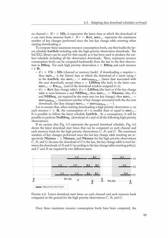
6.3. Adapting data download schedules on board
on channel r. If r ∈ Mb, it represents the latest time at which the download ofo can start from memory bank r. If r = Kct, mrco,r represents the maximumnumber of key changes performed since the last key change table resetting whenstarting downloading o.
To compute these maximum resource consumption levels, one rst builds the lat-est schedule LatSch including only the high priority observation downloads. eInCELL library can be used for that exactly as it has been used to produce the ear-liest schedule including all the observation downloads. en, maximum resourceconsumption levels can be computed backwardly from the last to the rst observa-tion in HSeq. For each high priority observation o ∈ HSeq and each resourcer ∈ R:
– if r ∈ Ch ∪Mb (channel or memory bank): if downloading o requires r,then mrco,r is the (latest) date at which the download of o starts using rin the LatSch; else mrco,r = mrcNHSeqo,r (latest date associated withthe next download), except when o = LHSeq (the last); in the latter case,mrco,r = Ewdwo (end of the download window assigned to o);
– if r = Kct (key change table): if o = LHSeq (the last) or if the key changetable is reset between o and NHSeqo, then mrco,r = Nkmax; else, if oand NHSeqo are required by the same user (no key change), then mrco,r =mrcNHSeqo,r (maximum number of key changes associated with the the nextdownload), else (key change) mrco,r = mrcNHSeqo,r − 1.
Let us assume that, when starting downloading a high priority observation o, oneach resource r ∈ R, the consumption of r is smaller than or equal to mrco,r .It is possible to follow the latest schedule LatSch. As a consequence, it will bepossible to perform NsHSeqo (download of o and of all the following high priorityobservations).
If we assume that Fig. 4.2 represents the ground download schedule, Fig. 6.6shows the latest download start times that can be computed on each channel andeach memory bank for the high priority observations C, B, and G. e maximumnumbers of key changes performed since the last key change table resetting are re-spectively Nkmax− 1, Nkmax, and Nkmax for the high priority observationsC, B, and G, because the download of G is the last, the key change table is reset be-tween the downloads of B and G (according to the key change table resetting policy),and C and B are required by two different users.
C2
C3
C1
G,2
G,4
G,3
B,5B,4
B,3
B,1C,3 B,2
C,5C,2
C,1
W1 (S1)W2 (S2)
C,4
s1 e1e2s2
High priority observations
t1
F . : Latest download start times on each channel and each memory bankcomputed on the ground for the high priority observations C, B, and G.
Once these maximum resource consumption levels have been computed, the
89
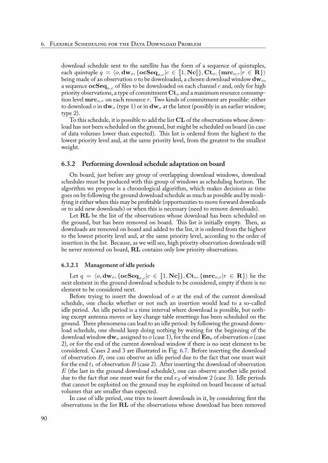
. F S D D P
download schedule sent to the satellite has the form of a sequence of quintuples,each quintuple q = ⟨o, dwo, ocSeqo,c|c ∈ J1, NcK, Cto, mrco,r|r ∈ R⟩being made of an observation o to be downloaded, a chosen download window dwo,a sequence ocSeqo,c of les to be downloaded on each channel c and, only for highpriority observations, a type of commitment Cto and a maximum resource consump-tion level mrco,r on each resource r. Two kinds of commitment are possible: eitherto download o in dwo (type 1) or in dwo at the latest (possibly in an earlier window;type 2).
To this schedule, it is possible to add the list CL of the observations whose down-load has not been scheduled on the ground, but might be scheduled on board (in caseof data volumes lower than expected). is list is ordered from the highest to thelowest priority level and, at the same priority level, from the greatest to the smallestweight.
6.3.2 Performing download schedule adaptation on boardOn board, just before any group of overlapping download windows, download
schedules must be produced with this group of windows as scheduling horizon. ealgorithm we propose is a chronological algorithm, which makes decisions as timegoes on by following the ground download schedule as much as possible and by modi-fying it either when this may be pro table (opportunities to move forward downloadsor to add new downloads) or when this is necessary (need to remove downloads).
Let RL be the list of the observations whose download has been scheduled onthe ground, but has been removed on board. is list is initially empty. en, asdownloads are removed on board and added to the list, it is ordered from the highestto the lowest priority level and, at the same priority level, according to the order ofinsertion in the list. Because, as we will see, high priority observation downloads willbe never removed on board, RL contains only low priority observations.
6.3.2.1 Management of idle periodsLet q = ⟨o, dwo, ocSeqo,c|c ∈ J1, NcK, Cto, mrco,r|r ∈ R⟩ be the
next element in the ground download schedule to be considered, empty if there is noelement to be considered next.
Before trying to insert the download of o at the end of the current downloadschedule, one checks whether or not such an insertion would lead to a so-calledidle period. An idle period is a time interval where download is possible, but noth-ing except antenna moves or key change table resettings has been scheduled on theground. ree phenomena can lead to an idle period: by following the ground down-load schedule, one should keep doing nothing by waiting for the beginning of thedownload window dwo assigned to o (case 1), for the end Eoo of observation o (case2), or for the end of the current download window if there is no next element to beconsidered. Cases 2 and 3 are illustrated in Fig. 6.7. Before inserting the downloadof observation B, one can observe an idle period due to the fact that one must waitfor the end t1 of observation B (case 2). After inserting the download of observationE (the last in the ground download schedule), one can observe another idle perioddue to the fact that one must wait for the end e2 of window 2 (case 3). Idle periodsthat cannot be exploited on the ground may be exploited on board because of actualvolumes that are smaller than expected.
In case of idle period, one tries to insert downloads in it, by considering rst theobservations in the list RL of the observations whose download has been removed
90
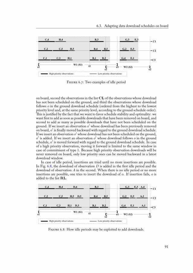
6.3. Adapting data download schedules on board
High priority observations Low priority observations
B,3
B,4 B,5
C1
B,1C3
B,2
C2
H,4
C,2
C,4
H,5
C,1
C,5
H,1
G,3
C,3 G,4 E,1
G,2
E,3
W1 (S1)
E,5
e2s1 W2 (S2)t1
s2e1
F . : Two examples of idle period
on board, second the observations in the list CL of the observations whose downloadhas not been scheduled on the ground, and third the observations whose downloadfollows o in the ground download schedule (ordered from the highest to the lowestpriority level and, at the same priority level, according to the ground schedule order).
is is justi ed by the fact that we want to favor schedule stability and optimality: wewant rst to add as soon as possible downloads that have been removed on board, andsecond to add as many as possible downloads that have not been scheduled on theground. If we insert an observation o′ whose download has been previously removedon board, o′ is nally moved backward with regard to the ground download schedule.If we insert an observation o′ whose download has not been scheduled on the ground,o′ is added. If we insert an observation o′ whose download follows o in the groundschedule, o′ is moved forward with regard to the ground download schedule. In caseof a high priority observation, moving it forward is limited to the same window incase of commitment of type 1. Because high priority observation downloads will benever removed on board, only low priority ones can be moved backward in a latestdownload window.
In case of idle period, insertions are tried until no more insertions are possible.In Fig. 6.8, the download of observation D is added in the rst idle period and thedownload of observation A in the second. When there is no idle period or no moreinsertions are possible, one tries to insert the download of o. If insertion fails, o isadded to the list RL.
High priority observations Low priority observations
B,3
B,1
B,5B,4C2
C3
C1C,4 H,4
B,2
C,5 H,5C,2
C,3 H,1C,1
G,2
G,4
G,3
E,5D,5
E,1
D,4
D,3
E,3 A,4
A,1
A,2
W2 (S2)e2
W1 (S1)s1 e1t1
s2
F . : How idle periods may be exploited to add downloads.
91
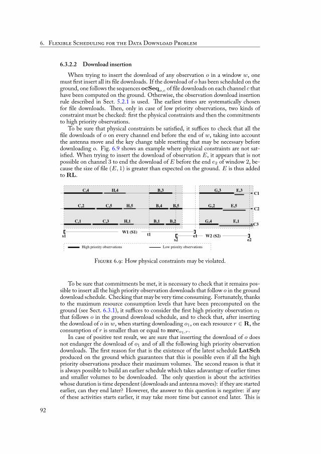
. F S D D P
6.3.2.2 Download insertionWhen trying to insert the download of any observation o in a window w, one
must rst insert all its le downloads. If the download of o has been scheduled on theground, one follows the sequences ocSeqo,c of le downloads on each channel c thathave been computed on the ground. Otherwise, the observation download insertionrule described in Sect. 5.2.1 is used. e earliest times are systematically chosenfor le downloads. en, only in case of low priority observations, two kinds ofconstraint must be checked: rst the physical constraints and then the commitmentsto high priority observations.
To be sure that physical constraints be satis ed, it suffices to check that all thele downloads of o on every channel end before the end of w, taking into account
the antenna move and the key change table resetting that may be necessary beforedownloading o. Fig. 6.9 shows an example where physical constraints are not sat-is ed. When trying to insert the download of observation E, it appears that is notpossible on channel 3 to end the download of E before the end e2 of window 2, be-cause the size of le (E, 1) is greater than expected on the ground. E is thus addedto RL.
High priority observations Low priority observations
B,4
B,1
B,3C1
C2B,5
B,2
H,4
C3H,1
E,3
H,5
E,1
G,3
E,5G,2
C,4
G,4C,1 C,3
C,2
W1 (S1)W2 (S2)
C,5
t1s1e2s2
e1
F . : How physical constraints may be violated.
To be sure that commitments be met, it is necessary to check that it remains pos-sible to insert all the high priority observation downloads that follow o in the grounddownload schedule. Checking that may be very time consuming. Fortunately, thanksto the maximum resource consumption levels that have been precomputed on theground (see Sect. 6.3.1), it suffices to consider the rst high priority observation o1that follows o in the ground download schedule, and to check that, after insertingthe download of o in w, when starting downloading o1, on each resource r ∈ R, theconsumption of r is smaller than or equal to mrco1,r .
In case of positive test result, we are sure that inserting the download of o doesnot endanger the download of o1 and of all the following high priority observationdownloads. e rst reason for that is the existence of the latest schedule LatSchproduced on the ground which guarantees that this is possible even if all the highpriority observations produce their maximum volumes. e second reason is that itis always possible to build an earlier schedule which takes adavantage of earlier timesand smaller volumes to be downloaded. e only question is about the activitieswhose duration is time dependent (downloads and antenna moves): if they are startedearlier, can they end later? However, the answer to this question is negative: if anyof these activities starts earlier, it may take more time but cannot end later. is is
92
6.3. Adapting data download schedules on board
obvious for download durations: if it is possible to download a le f from t1 to t2and if we start downloading f at t′
1 < t1, in the worst case, nothing is downloadedfrom t′
1 to t1 and the le f is downloaded from t1 to t2; as a consequence, f willbe downloaded at t2 at the latest. is is also true for antenna move durations if weassume that the antenna is more agile than the satellite (able to be trained on a stationin spite of any satellite attitude movement): if it is possible to move the antenna fromstation s1 to station s2 from t1 to t2 and if we start moving the antenna at t′
1 < t1,in the worst case, the satellite remains trained on station s1 from t′
1 to t1 and theantenna movement is performed from t1 to t2; as a consequence, the movement endsat t2 at the latest.
However, in case of negative test result, for two reasons, we are not sure thatinserting the download of o really endangers the download of o1 and of all the fol-lowing high priority observation downloads. e rst reason is that the maximumresource consumption levels have been computed on the ground with the assumptionof maximum volumes for all the high priority observations. e second is that someof the high priority observation downloads that follow o in the ground downloadschedule may have been moved forward and have no longer to be considered. As aconsequence, on every resource r, mrco1,r is pessimistic: it is a lower bound on theactual maximum resource consumption levels.
If we really want to know whether or not inserting the download of o allows com-mitments to be met, an option is to recompute the maximum resource consumptionlevels for all the future high priority observations with the information about theactual volumes for those that are nished, as well as the information about forwardmoves. Because this may be time consuming, we propose a kind of lazy lookahead.Let NsHSeqo1 = [o1, . . . , on] be the sequence of the high priority observationdownloads that follow o in the ground download schedule:
– at the rst lookahead step, we check that, by inserting the download of o and o1(with the new information about o1), when starting downloading o2, on eachresource r ∈ R, the consumption of r is smaller than or equal to mrco2,r ; incase of positive answer, inserting the download of o is possible and if, on everyresource r ∈ R, the resource consumption level when starting downloading o1is greater than mrco1,r , it is used to update mrco1,r (less pessimistic lowerbound on the actual maximum resource consumption levels); in case of negativeanswer, we can still check further;
– if necessary, at the ith lookahead step (i < n), we check that, by insertingthe download of o and o1, o2, …, and oi (with the new information about o1,o2, …, and oi), when starting downloading oi+1, on each resource r ∈ R,the consumption of r is smaller than or equal to mrcoi+1,r ; in case of pos-itive answer, inserting the download of o is possible and, for each observa-tion oj | 1 ≤ j ≤ i, if, on every resource r ∈ R, the resource consumptionlevel when starting downloading oj is greater than mrcoj ,r , it is used to up-date mrcoj ,r (less pessimistic lower bound on the actual maximum resourceconsumption levels); in case of negative answer, we can still check further byincrementing i;
– if necessary, at the last lookahead step, we check that it is possible to inserto and o1, o2, …, and on (with the new information about o1, o2, …, andon); in case of positive answer, inserting o is possible and, for each observationoi | 1 ≤ i ≤ n, if, on every resource r ∈ R, resource consumption level whenstarting downloading oi is greater than mrcoi,r , it is used to update mrcoi,r
(less pessimistic lower bound on the actual maximum resource consumptionlevels); in case of negative answer, inserting the download of o is de nitely
93

. F S D D P
impossible and o is added to RL.Performing lookahead until i = n may be time consuming too. It must be how-
ever stressed, on the one hand, that lookahead may stop earlier in case of a positiveanswer and, on the other hand, it may be safely stopped at any step in case of negativeanswer: the download of o is not inserted and o added to RL, even if its insertionwould have been nally possible. In any case, high priority downloads are not en-dangered. If lookahead is never stopped, it is said to be complete. Otherwise, it issaid to be incomplete.
Fig. 6.10 shows an example where future high priority observation downloadsmight be endangered. When trying to insert the download of observation H , itappears that is not possible on channel 2 to start the download of B (the rst highpriority observation download that follows H in the ground download schedule)before its latest download start time, because the size of le (H, 5) is greater thanexpected on the ground.
High priority observations Low priority observations
C1
C3
C2B,5
B,3
B,2
B,4
C,4
B,1
C,5C,2
C,3C,1
H,5
H,4
W1 (S1)
H,1
e2W2 (S2)e1s1
s2
t1
F . : How high priority observation downloads might be endangered.
At the rst lookahead step, nothing changes because observation B ends dur-ing window 1 and maximum volumes are assumed on board as well on the ground(no new information available on board about B). However, at the second and lastlookahead step, it appears in Fig. 6.11 that, because of the actual volumes of ob-servation G (the second and last high priority observation download that follows Hin the ground download schedule) it is nally possible to insert H , B, and G. edownload of H is thus inserted.
Fig. 6.12 gives a more macroscopic view of the onboard repair procedure. ereare 8 observations to be downloaded. Only 6 of them have been scheduled in theground plan (o1, o2, o3, o4, o7, o8). Maximum volumes have been considered forhigh-priority observations and average for low-priority observations. Only lateststart dates are shown at each iteration (and not for each channel). On board, onlytwo volumes are different with respect to the assumptions made on the ground: o1is lower than maximum (green) and o7 is higher than average (red). e onboardprocedure follows the original ground plan. It manages to insert the download ofobservation o5 by taking advantage of an idle period created by the smaller volumefor o1. At iteration 3, it tries to insert low-priority observation download o7 but thelatest start date check shows that it may endanger future high-priority downloads.
en, at iteration 4, a lookahead is performed and because the volume of o3 and o4have not changed, o7 is discarded. At iteration 5, the download of o6 is introduced
94
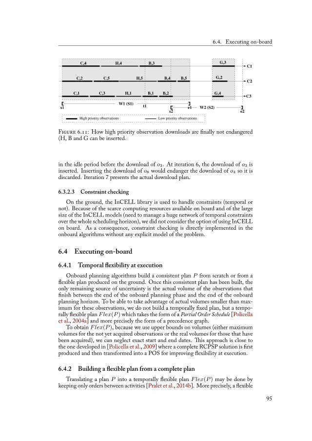
6.4. Executing on-board
High priority observations Low priority observations
C2
C3
C1
C,2 C,5
C,4
C,3
H,4
C,1 H,1
W1 (S1)
H,5
e2s1 W2 (S2)t1
s2e1
G,2
G,4
G,3
B,1 B,2
B,3
B,4 B,5
F . : How high priority observation downloads are nally not endangered(H, B and G can be inserted.
in the idle period before the download of o3. At iteration 6, the download of o3 isinserted. Inserting the download of o8 would endanger the download of o4 so it isdiscarded. Iteration 7 presents the actual download plan.
6.3.2.3 Constraint checkingOn the ground, the InCELL library is used to handle constraints (temporal or
not). Because of the scarce computing resources available on board and of the largesize of the InCELL models (need to manage a huge network of temporal constraintsover the whole scheduling horizon), we did not consider the option of using InCELLon board. As a consequence, constraint checking is directly implemented in theonboard algorithms without any explicit model of the problem.
6.4 Executing on-board
6.4.1 Temporal exibility at executionOnboard planning algorithms build a consistent plan P from scratch or from a
exible plan produced on the ground. Once this consistent plan has been built, theonly remaining source of uncertainty is the actual volume of the observations thatnish between the end of the onboard planning phase and the end of the onboard
planning horizon. To be able to take advantage of actual volumes smaller than max-imum for these observations, we do not build a temporally xed plan, but a tempo-rally exible plan F lex(P ) which takes the form of a Partial Order Schedule [Policellaet al., 2004a] and more precisely the form of a precedence graph.
To obtain F lex(P ), because we use upper bounds on volumes (either maximumvolumes for the not yet acquired observations or the real volumes for those that havebeen acquired), we can neglect exact start and end dates. is approach is close tothe one developed in [Policella et al., 2009] where a complete RCPSP solution is rstproduced and then transformed into a POS for improving exibility at execution.
6.4.2 Building a exible plan from a complete planTranslating a plan P into a temporally exible plan F lex(P ) may be done by
keeping only orders between activities [Pralet et al., 2014b]. More precisely, a exible
95
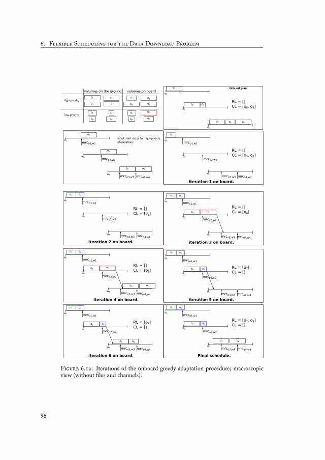
. F S D D P
F . : Iterations of the onboard greedy adaptation procedure; macroscopicview (without les and channels).
96
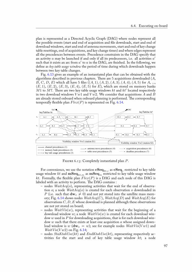
6.4. Executing on-board
plan is represented as a Directed Acyclic Graph (DAG) where nodes represent allthe possible events (start and end of acquisition and le downloads, start and end ofdownload windows, start and end of antenna movements, start and end of key changetable resettings, end of acquisitions, and key change times) and where edges representall the precedences between events. Precedence constraints in the DAG specify thatan activity a may be launched if and only if all its predecessors, i.e. all activities a′
such that it exists an arc from a′ to a in the DAG, are nished. In the following, wede ne as key table usage window the period of time during which downloads happenbetween two key table changes.
Fig. 6.13 gives an example of an instantiated plan that can be obtained with thealgorithms described in previous chapters. ere are 5 acquisitions downloaded (A,B, C, D, E) which all have 5 les ((A, 1), (A, 2), (A, 3), (A, 4), (A, 5) for A, ...,(E, 1), (E, 2), (E, 3), (E, 4), (E, 5) for E), which are stored on memory banksM1 to M7. ere are two key table usage windows kt and kt′ located respectivelyin two download windows V w1 and V w2. We consider that acquisitions A and Bare already stored onboard when onboard planning is performed. e correspondingtemporally exible plan F lex(P ) is represented on Fig. 6.14.
F . : Completely instantiated plan P .
For convenience, we use the notation cSeqkt,c as cSeqc restricted to key tableusage window kt and mSeqkt,m as mSeqm restricted to key table usage windowkt. Formally, the exible plan F lex(P ) is a DAG and each node of this DAG islabeled with an activity to perform. e DAG contains :
– nodes WaitAcq(o), representing activities that wait for the end of observa-tion o; a node WaitAcq(o) is created for each observation o downloaded inP (i.e. such that dwo = 0) and not yet stored into the satellite mass mem-ory; Fig. 6.14 shows nodes WaitAcq(C), WaitAcq(D) and WaitAcq(E) forobservations C, D, E whose download is planned although these observationsare not yet stored on board;
– nodes WaitVis(w), representing activities that wait for the beginning of adownload window w; a node WaitVis(w) is created for each download win-dow w used in P for downloading acquisitions, that is for each download win-dow w such that there exists at least one acquisition a whose assigned down-load window is w (dwa = w); see for example nodes WaitVis(V w1) andWaitVis(V w2) on Fig. 6.14;
– nodes StaKtabUse(kt) and EndKtabUse(kt), representing respectively ac-tivities for the start and end of key table usage window kt; a node
97
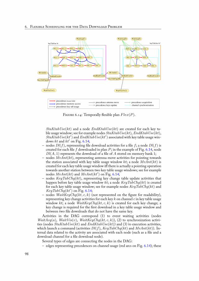
. F S D D P
F . : Temporally exible plan F lex(P ).
StaKtabUse(kt) and a node EndKtabUse(kt) are created for each key ta-ble usage window; see for example nodes StaKtabUse(kt), EndKtabUse(kt),StaKtabUse(kt′) and EndKtabUse(kt′) associated with key table usage win-dows kt and kt′ on Fig. 6.14;
– nodes Dl(f), representing le download activities for a le f ; a node Dl(f) iscreated for each le f downloaded in plan P ; in the example of Fig. 6.14, nodeDl(A, 1) represents the download of a le of A stored on memory bank 1;
– nodes MvAnt(kt), representing antenna move activities for pointing towardsthe station associated with key table usage window kt; a node MvAnt(kt) iscreated for each key table usage window iff there is actually a pointing operationtowards another station between two key table usage windows; see for examplenodes MvAnt(kt) and MvAnt(kt′) on Fig. 6.14;
– nodes KeyTabChg(kt), representing key change table update activities thathappen before key table usage window kt; a node KeyTabChg(kt) is createdfor each key table usage window; see for example nodes KeyTabChg(kt) andKeyTabChg(kt′) on Fig. 6.14;
– nodes WaitKeyChg(kt, c, k) (not represented on the gure for readability),representing key change activities for each key k on channel c in key table usagewindow kt; a node WaitKeyChg(kt, c, k) is created for each key change; akey change is required for the rst download in a key table usage window andbetween two le downloads that do not have the same key.
Activities in the DAG correspond (1) to event waiting activities (nodesWaitAcq(a), WaitVis(v), WaitKeyChg(kt, c, k)), (2) to synchronization activi-ties (nodes StaKtabUse(kt) and EndKtabUse(kt)) and (3) to execution activities,which launch a command (activities Dl(f), KeyTabChg(kt) and MvAnt(kt)). In-ternal data related to the activity are associated with each node (such as a le and adownload channel for a le download node).
Several types of edges are connecting the nodes in the DAG:– edges representing precedences on channel usage (red arcs on Fig. 6.14); these
98
6.4. Executing on-board
edges between download nodes Dl(.) are obtained directly from sequencescSeqkt,c for each channel c ∈ J1, NcK and each key table usage windowkt;
– edges representing precedences for reading access to memory banks (deep blueedges on Fig. 6.14); these edges between download nodes Dl(.) are obtaineddirectly from sequences mSeqkt,m for each memory bank m ∈ J1, NmK andeach key table usage window kt;
– edges representing precedences between observation acquisition and download(green edges on Fig. 6.14); for each observation a not yet stored on board andwhose download is planned in P , an edge from WaitAcq(a) to Dl(f) is addedfor each le f of observation a;
– edges representing precedences between start dates of download windows andstart dates of key table usage windows (dotted edges on Fig. 6.14); for eachkey table usage window kt in download window w, a edge is added from nodeWaitVis(w) to node StaKtabUse(kt);
– edges representing precedences between the start of key table usage windowsand the start of le downloads (light blue edges on Fig. 6.14); for each key tableusage window kt and each channel c ∈ J1, NcK, an edge is added from nodeStaKtabUse(kt) to node Dl(f) with f the rst le downloaded in sequencecSeqkt,c (if it exists);
– edges representing precedences between the end of le downloads on channelsand the end of key table usage windows (light blue edges on Fig. 6.14); for eachkey table usage window kt and each channel c ∈ J1, NcK, an edge is addedfrom node Dl(f) to node EndKtabUse(kt) with f the last le downloaded insequence cSeqkt,c (if it exists);
– edges representing precedences between the end of key table usage windowsand the start of antenna movements for pointing towards the station linkedto the next key table usage window (double line edges on Fig. 6.14); for eachcouple of adjacent key table usage windows (kti−1, kti), an edge is added fromnode EndKtabUse(kti−1) to node MvAnt(kti) (if it exists);
– edges representing precedences between the end of antenna movements andthe start of key table usage windows (double line edges on Fig. 6.14); for eachkey table usage window kt, an edge is added from node MvAnt(kt) to nodeStaKtabUse(kt);
– edges representing precedences between the end of key table usage windowsand key change tables updates (black line edges on Fig. 6.14); for each coupleof adjacent key table usage windows (kti−1, kti), an edge is added from nodeEndKtabUse(kti−1) to node KeyTabChg(kti);
– edges representing precedences between the end of key change tables updatingand the start of key table usage windows (black line on Fig. 6.14); for each keytable usage window kt, an edge is added from node KeyTabChg(kt) to nodeStaKtabUse(kt);
– edges (not shown on the gure) representing precedences between key changesand le downloads; for each key table usage window kt and each channelc ∈ J1, NcK, an edge is added from node WaitKeyChg(kt, c, k) to nodeDl(f) with f the le such that the kth key change has to be done before fis downloaded.
99
. F S D D P
6.4.3 Executione precedence graph is represented as a Directed Acyclic Graph G = (V, E)
with V a set of nodes and E a set of pairs of nodes called edges. A graph is acyclic iff,starting from any node, there is no path leading to that node. A node x is a prede-cessor of node y iff there exists an arc (x, y). A node may have several predecessors.
In this graph, we can distinguish controllable events (starts of activities which areunder the control of the executive) and uncontrollable events (ends of activities whichare under the control of the environment). With each node is associated a counterrepresenting the number of its predecessors that are not nished yet.
is precedence graph is then executed with the following policy: any node isactivated as soon as all its parents in the graph are executed, until all the events areexecuted. is policy may allow observations to be downloaded earlier than expectedin the plan.
For three reasons, no event in the precedence graph can be triggered later thanexpected in the download schedule. e rst reason is that the download schedulesare pessimistic (assumption of maximum volumes for all the observations that are notnished yet). e second is, even if some activity durations (downloads and antenna
moves) are time-dependent, if these activities start earlier, they may take more timebut cannot end later (see Sect.6.3.2.2). e third is that each event is triggered assoon as all its predecessors in the graph have been triggered. is guarantees that allthe precedence constraints that have been checked in the pessimistic schedule willbe satis ed at execution. In particular, no le download will end after the end of thedownload window it has been assigned to.
Last, to model a download plan without temporal exibility, the only thing todo is to add temporal waiting nodes in the DAG for each activity. at way, nodownload or antenna transition is moved forward.
6.5 Experiments
6.5.1 Approaches to be comparedTo assess the positive impact of sharing decision-making between ground and on-
board, we implemented and compared the following four approaches in the simulatorpresented in Appendix A:
1. scheduling on the ground (Ground) : download scheduling is performed onthe ground with maximum volumes for all the observations, using an SWOalgorithm built on top of a non-chronological greedy algorithm, as describedin Sect. 5.3; this schedule is then executed on board; the only difference withthe currently operational approach is that a precedence DAG built from theschedule allows temporal exibility to be exploited on board and downloadsto be started earlier than in the pessimistic ground schedule, as described inSect. 6.4; this slightly favors the ground approach in terms of information age;
2. scheduling on board (Board) : download scheduling is performed on boardfrom scratch before each group of overlapping download windows with ex-act volumes for the observations that are already nished and maximum vol-umes for the others, using a chronological greedy algorithm, as described inSect. 5.2.2; as in the previous approach, a precedence DAG built from theschedule allows temporal exibility to be exploited;
100
6.5. Experiments
3. download scheduling is performed on the ground with maximum volumes forthe high-priority observations and expected volumes for the others, using anSWO algorithm built on top of a non-chronological greedy algorithm, as inthe ground approach; then, download scheduling is performed on board be-fore each group of overlapping download windows with exact volumes for theobservations that are already nished and maximum volumes for the others,by following and adapting the ground schedule, as described in Sect. 6.3; asin the previous approaches, a precedence DAG built from the schedule allowstemporal exibility to be exploited; two variants of the onboard adaptationmechanisms have been implemented:
a) a very simple board adaptation mechanism (SimpleRepair): downloads ofany priority level are removed from the ground schedule when they arephysically unfeasible; this means that only physical constraints are con-sidered; commitments to high priority observations are not considered;
b) an intelligent board adaptation mechanism (SmartRepair): low prioritydownloads are removed from the schedule either when they are phys-ically unfeasible or when they prevent future high priority downloadsfrom being performed; downloads are also added or moved forward whenpossible; this means that commitments to high priority observations, aswell as physical constraints, are considered; to check that commitmentscan be met, a complete lookahead mechanism is used; see Sect. 6.3 fordetails.
6.5.2 ScenariosWe use two realistic scenarios provided by Airbus Defence and Space (see their
characteristics in Table 6.1). Both scenarios have been produced from the same ac-tual one-day observation schedule built for a currently operational Earth-observingsatellite (about 14 satellite revolutions around Earth over the whole day). ey dif-fer from each other according to the number of available ground reception stations:Scenario 1 (the least constrained) involves a large number of ground reception sta-tions (23) resulting in many download windows (115), whereas Scenario 2 (the mostconstrained) involves a small number of ground reception stations (3) resulting inonly few download windows (20). ey also differ in the way observations are dis-tributed between users and priority levels: 275 (resp. 247) high priority observationsand 1089 (resp. 1117) low priority observations for Scenario 1 (resp. 2). Actual levolumes are randomly generated between Vmax/4 and Vmax, with Vmax themaximum le volume. 15 instances of actual volumes have been randomly generatedand all the results are mean values over these 15 instances. Experiments were run ona Xeon 4-core 3GHz cpu with 8GB RAM, with Ubuntu 12.04 LTS.
6.5.3 Evaluation criteriaExecution results are compared according to several criteria:1. the number of observation downloads, at each priority level;2. the mean information age over all the downloaded observations, at each pri-
ority level;3. the global criterion described in Sect. 4.2.4.2, at each priority level, computed
with a sharing parameter equal to −3; because this complex criterion aggre-gates many different characteristics of a schedule (weights of the downloaded
101

. F S D D P
Scenario 1 Scenario 2# of memory banks 5 5
# of channels 3 3# of ground reception stations 23 3
# of download windows 115 20# of users 5 5
# of priority levels 2 2# of observations 1364 1364
# of high-priority observations 275 247# of low-priority observations 1089 1117
# of generated les 6820 6820# of volume instances 15 15
Table 6.1: Scenario characteristics.
observations, information age, sharing between users), its exact value has noreal importance; what is important is only the fact that it may be higher withan approach than with another one;
4. the mean computing time consumed by onboard scheduling, over the succes-sive groups of overlapping download windows;
5. only for the third and fourth approaches, the differences between the groundand onboard schedules: number of downloads that are added, removed, movedforward, and moved backward, at each priority level.e rst three criteria measure the quality of the execution results. e fourth
one measures the cost of onboard scheduling. e fth one measures the stability ofthe onboard schedules with regard to the ground ones.
6.5.4 Result analysisNumber of observation downloads With regard to the number of downloads (seeFig. 6.15), whatever the scenario is, high priority observations are all downloaded,except with the SimpleRepair approach which does not check whether or not futurehigh priority downloads are endangered when inserting low priority ones. Low pri-ority observations are all downloaded on Scenario 1, but not on Scenario 2. On thelatter scenario (the most constrained), only the SmartRepair and Board approachesallow all of them to be downloaded.
Mean information age Signi cant differences appear in Fig. 6.16 only for low pri-ority observations on Scenario 2 (the most constrained). Mean information age de-creases from the Ground approach to the Board one, suggesting that the higher exi-bility in onboard decision-making, the lower resulting information age.
Global criterion With regard to the global criterion, Fig. 6.17 shows that, for highpriority observations on Scenario 1, the Ground and SmartRepair approaches are bet-ter than the SimpleRepair and Board approaches. For the SimpleRepair approach, thiscan be explained by the fact that it removes high priority downloads. For the Board
102
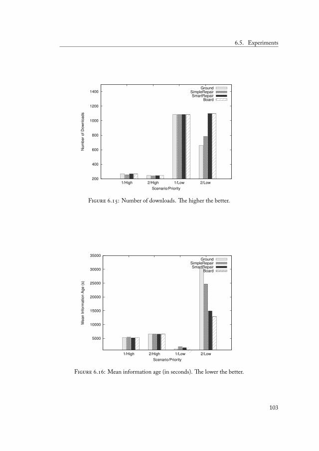
6.5. Experiments
200
400
600
800
1000
1200
1400
1/High 2/High 1/Low 2/Low
NumberofDownloads
Scenario/Priority
GroundSimpleRepairSmartRepair
Board
F . : Number of downloads. e higher the better.
5000
10000
15000
20000
25000
30000
35000
1/High 2/High 1/Low 2/Low
MeanInform
ationAge(s)
Scenario/Priority
GroundSimpleRepairSmartRepair
Board
F . : Mean information age (in seconds). e lower the better.
103
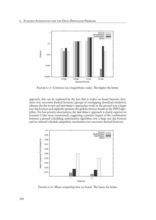
. F S D D P
0.0001
0.001
0.01
0.1
1
1/High 2/High 1/Low 2/Low
Crite
rio
n
Scenario/Priority
GroundSimpleRepairSmartRepair
Board
F . : Criterion (on a logarithmic scale). e higher the better.
approach, this can be explained by the fact that it makes on board heuristic deci-sions over successive limited horizons (groups of overlapping download windows),whereas the the Ground and SmartRepair approaches work on the ground over a largerone-day horizon and explicitly optimize the global criterion thanks to the SWO algo-rithm. For low priority observations, the SmartRepair approach is clearly superior onScenario 2 (the most constrained), suggesting a positive impact of the combinationbetween a ground scheduling optimization algorithm over a large one-day horizonand an onboard schedule adaptation mechanism over successive limited horizons.
0.01
0.02
0.03
0.04
0.05
0.06
0.07
0.08
0.09
0.1
1 2
MeanComputingTimeOnboard(s)
Scenario
GroundSimpleRepairSmartRepair
Board
F . : Mean computing time on board. e lower the better.
104
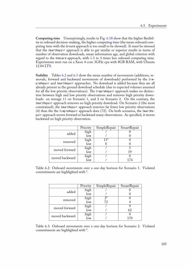
6.5. Experiments
Computing time Unsurprisingly, results in Fig. 6.18 show that the higher exibil-ity in onboard decision-making, the higher computing time (the mean onboard com-puting time with the Ground approach is too small to be showed). It must be stressedthat the SmartRepair approach is able to get similar or superior results in terms ofnumber of observation downloads, mean information age, and global criterion withregard to the Onboard approach, with 1.5 to 3 times less onboard computing time.Experiments were run on a Xeon 4-core 3GHz cpu with 8GB RAM, with Ubuntu12.04 LTS.
Stability Tables 6.2 and 6.3 show the mean number of movements (additions, re-movals, forward and backward movements of downloads) performed by the Sim-pleRepair and SmartRepair approaches. No download is added because they are allalready present in the ground download schedule (due to expected volumes assumedfor all the low priority observations). e SimpleRepair approach makes no distinc-tion between high and low priority observations and removes high priority down-loads: on average 11 on Scenario 1, and 2 on Scenario 2. On the contrary, theSmartRepair approach removes no high priority download. On Scenario 2 (the mostconstrained), the SmartRepair approach removes far fewer low priority observations(4) than the the SimpleRepair approach does (72). On both scenarios, the SmartRe-pair approach moves forward or backward many observations. As speci ed, it movesbackward no high priority observation.
Priority SimpleRepair SmartRepairadded high / 0
low / 0removed high 11* 0
low 0 0moved forward high / 5
low / 19moved backward high / 0
low / 174
Table 6.2: Onboard movements over a one-day horizon for Scenario 1. Violatedcommitments are highlighted with *.
Priority SimpleRepair SmartRepairadded high / 0
low / 0removed high 2* 0
low 72 4moved forward high / 9
low / 62moved backward high / 0
low / 170
Table 6.3: Onboard movements over a one-day horizon for Scenario 2. Violatedcommitments are highlighted with *.
105
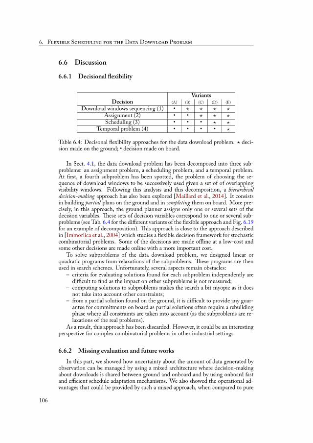
. F S D D P
6.6 Discussion
6.6.1 Decisional exibility
VariantsDecision (A) (B) (C) (D) (E)
Download windows sequencing (1) • ⋆ ⋆ ⋆ ⋆Assignment (2) • • ⋆ ⋆ ⋆Scheduling (3) • • • ⋆ ⋆
Temporal problem (4) • • • • ⋆
Table 6.4: Decisonal exibility approaches for the data download problem. ⋆ deci-sion made on the ground; • decision made on board.
In Sect. 4.1, the data download problem has been decomposed into three sub-problems: an assignment problem, a scheduling problem, and a temporal problem.At rst, a fourth subproblem has been spotted, the problem of choosing the se-quence of download windows to be successively used given a set of of overlappingvisibility windows. Following this analysis and this decomposition, a hierarchicaldecision-making approach has also been explored [Maillard et al., 2014]. It consistsin building partial plans on the ground and in completing them on board. More pre-cisely, in this approach, the ground planner assigns only one or several sets of thedecision variables. ese sets of decision variables correspond to one or several sub-problems (see Tab. 6.4 for the different variants of the exible approach and Fig. 6.19for an example of decomposition). is approach is close to the approach describedin [Immorlica et al., 2004] which studies a exible decision framework for stochasticcombinatorial problems. Some of the decisions are made offline at a low-cost andsome other decisions are made online with a more important cost.
To solve subproblems of the data download problem, we designed linear orquadratic programs from relaxations of the subproblems. ese programs are thenused in search schemes. Unfortunately, several aspects remain obstacles:
– criteria for evaluating solutions found for each subproblem independently aredifficult to nd as the impact on other subproblems is not measured;
– computing solutions to subproblems makes the search a bit myopic as it doesnot take into account other constraints;
– from a partial solution found on the ground, it is difficult to provide any guar-antee for commitments on board as partial solutions often require a rebuildingphase where all constraints are taken into account (as the subproblems are re-laxations of the real problems).
As a result, this approach has been discarded. However, it could be an interestingperspective for complex combinatorial problems in other industrial settings.
6.6.2 Missing evaluation and future worksIn this part, we showed how uncertainty about the amount of data generated by
observation can be managed by using a mixed architecture where decision-makingabout downloads is shared between ground and onboard and by using onboard fastand efficient schedule adaptation mechanisms. We also showed the operational ad-vantages that could be provided by such a mixed approach, when compared to pure
106
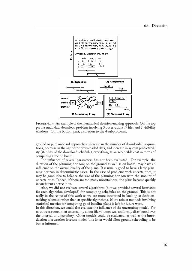
6.6. Discussion
F . : An example of the hierarchical decision-making approach. On the toppart, a small data download problem involving 3 observations, 9 les and 2 visibilitywindows. On the bottom part, a solution to the 4 subproblems.
ground or pure onboard approaches: increase in the number of downloaded acquisi-tions, decrease in the age of the downloaded data, and increase in system predictabil-ity (stability of the download schedule), everything at an acceptable cost in terms ofcomputing time on board.
e in uence of several parameters has not been evaluated. For example, theduration of the planning horizon, on the ground as well as on board, may have anin uence on the overall quality of the plans. It is usually good to have a large plan-ning horizon in deterministic cases. In the case of problems with uncertainties, itmay be good idea to balance the size of the planning horizon with the amount ofuncertainties. Indeed, if there are too many uncertainties, the plans become quicklyinconsistent at execution.
Also, we did not evaluate several algorithms (but we provided several heuristicsfor each algorithm developed) for computing schedules on the ground. is is notreally in the scope of this work as we are more interested in looking at decision-making schemes rather than at speci c algorithms. More robust methods involvingstatistical metrics for computing good baseline plans is left for future work.In this direction, we could also evaluate the in uence of the uncertainty model. Fornow, we assumed that uncertainty about le volumes was uniformly distributed overthe interval of uncertainty. Other models could be evaluated, as well as the intro-duction of a weather forecast model. e latter would allow ground scheduling to bebetter informed.
107


Part III
Building conditional acquisition schedules
109

IntroductionIn the previous part, we described how exible download schedules are produced
on the ground when volumes are uncertain, together with commitments to high-priority data downloads. ese schedules are then adapted on board when exactvolumes are known. e onboard adaptation process guarantees that ground com-mitments to high-priority downloads be satis ed, but guarantees nothing about low-priority downloads. It only tries to perform the latter as well as possible. With suchan approach, the onboard adaptation process remains computationally light and themain computing effort is supported by the ground.
In this chapter, we switch to observation scheduling. More precisely, we presentan approach that has been developed to perform observation scheduling under un-certainty about the real energy level available on board at execution time. In this ap-proach, conditional observation schedules are produced on the ground where energylevels are uncertain, together with commitments to high priority observations. eonboard adaptation process guarantees that ground commitments to high-priorityobservations be satis ed: they will be performed exactly as foreseen in the groundschedule. However, it guarantees nothing about low-priority observations: each ofthem will be performed if and only if the current level of energy allows it and allowsall the future high-priority observations to be performed as well.
is part of the work has been presented at the IJCAI’15 International Workshopon Planning & Scheduling for Space (IWPSS’15) [Maillard et al., 2015b].

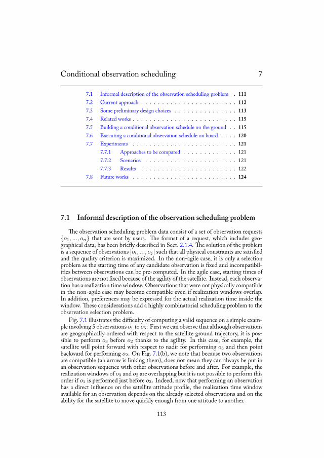
Conditional observation scheduling 7
7.1 Informal description of the observation scheduling problem . 1117.2 Current approach . . . . . . . . . . . . . . . . . . . . . . . 1127.3 Some preliminary design choices . . . . . . . . . . . . . . . 1137.4 Related works . . . . . . . . . . . . . . . . . . . . . . . . . 1157.5 Building a conditional observation schedule on the ground . . 1157.6 Executing a conditional observation schedule on board . . . . 1207.7 Experiments . . . . . . . . . . . . . . . . . . . . . . . . . 121
7.7.1 Approaches to be compared . . . . . . . . . . . . . 1217.7.2 Scenarios . . . . . . . . . . . . . . . . . . . . . . 1217.7.3 Results . . . . . . . . . . . . . . . . . . . . . . . 122
7.8 Future works . . . . . . . . . . . . . . . . . . . . . . . . . 124
7.1 Informal description of the observation scheduling problem
e observation scheduling problem data consist of a set of observation requestso1, ..., on that are sent by users. e format of a request, which includes geo-graphical data, has been brie y described in Sect. 2.1.4. e solution of the problemis a sequence of observations [oi, ..., oj ] such that all physical constraints are satis edand the quality criterion is maximized. In the non-agile case, it is only a selectionproblem as the starting time of any candidate observation is xed and incompatibil-ities between observations can be pre-computed. In the agile case, starting times ofobservations are not xed because of the agility of the satellite. Instead, each observa-tion has a realization time window. Observations that were not physically compatiblein the non-agile case may become compatible even if realization windows overlap.In addition, preferences may be expressed for the actual realization time inside thewindow. ese considerations add a highly combinatorial scheduling problem to theobservation selection problem.
Fig. 7.1 illustrates the difficulty of computing a valid sequence on a simple exam-ple involving 5 observations o1 to o5. First we can observe that although observationsare geographically ordered with respect to the satellite ground trajectory, it is pos-sible to perform o3 before o2 thanks to the agility. In this case, for example, thesatellite will point forward with respect to nadir for performing o3 and then pointbackward for performing o2. On Fig. 7.1(b), we note that because two observationsare compatible (an arrow is linking them), does not mean they can always be put inan observation sequence with other observations before and after. For example, therealization windows of o3 and o2 are overlapping but it is not possible to perform thisorder if o1 is performed just before o3. Indeed, now that performing an observationhas a direct in uence on the satellite attitude pro le, the realization time windowavailable for an observation depends on the already selected observations and on theability for the satellite to move quickly enough from one attitude to another.
113
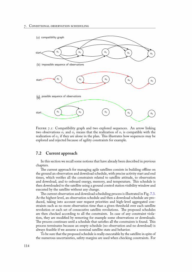
. C
F . : Compatibility graph and two explored sequences. An arrow linkingtwo observations oi and oj means that the realization of oi is compatible with therealization of oj if they are alone in the plan. is illustrates how sequences may beexplored and rejected because of agility constraints for example.
7.2 Current approachIn this section we recall some notions that have already been described in previous
chapters.e current approach for managing agile satellites consists in building offline on
the ground an observation and download schedule, with precise activity start and endtimes, which veri es all the constraints related to satellite attitude, to observationand download, and to onboard energy, memory, and temperature. is schedule isthen downloaded to the satellite using a ground control station visibility window andexecuted by the satellite without any change.
e current observation and download scheduling process is illustrated in Fig. 7.3.At the highest level, an observation schedule and then a download schedule are pro-duced, taking into account user request priorities and high-level aggregated con-straints such as no more observation time than a given threshold over each satelliterevolution or each set of consecutive satellite revolutions. e proposed schedulesare then checked according to all the constraints. In case of any constraint viola-tion, they are modi ed by removing for example some observations or downloads.
e process continues until a schedule that satis es all the constraints is found. isprocess terminates because an empty schedule (no observation and no download) isalways feasible if we assume a nominal satellite state and behavior.
To be sure that the proposed schedule is really executable by the satellite in spite ofthe numerous uncertainties, safety margins are used when checking constraints. For
114

7.3. Some preliminary design choices
example, the expected energy production and consumption rates are replaced by min-imum production and maximum consumption rates, resulting in harder constraints.
ese margins are used in high-level constraint checking phases. In Tab. 7.1, wecan see that the proportion of accepted observations over an initial pool of observa-tion requests is low (about 14%). Among the causes of rejection, about 34% are dueto energy and temperature high-level constraints. In Fig. 7.2, we can see the greatdifference between the expected energy pro le computed with margins (in green)and the real onboard pro le (in black). ese facts motivate a more exible decision-making approach to deal with these constraints. In this chapter, we focus only on theuncertainty about the onboard energy (uncertain productions and consumptions).
F . : Satellite energy pro les (in percentage of the maximum energy levelEmax) over a 24-hour scenario. e green line is the rst ground prediction withmargins produced by the current approach. e black line represents the actual en-ergy pro le resulting from the onboard execution of a conditional schedule. e redline is the minimum level of energy Emin, equal to 0.85 · Emax.
7.3 Some preliminary design choicesIn the previous part, a exible download scheduling approach has been proposed
to deal with the uncertainty about the volume of data generated by observations.Roughly speaking, this approach replaces the ground checking of the download andmemory constraints by a lighter checking which considers only high priority down-loads. For low-priority downloads, decision is delayed online on board and allows theground download schedule to be modi ed while guaranteeing ground commitmentsto high-priority downloads.
Our objective is to extend such an approach by proposing a exible observationscheduling approach to deal with uncertainty about energy production and consump-tion. Whereas we focus on energy in this chapter, the approach could be applied totemperature constraints.
accepted ∼ 14%rejected - kinematic con icts (agility constraints) ∼ 51%rejected - energy high-level constraints ∼ 25%rejected - temperature high-level constraints ∼ 9%rejected - other constraints ∼ 1%
Table 7.1: Causes of observation rejection in the planning process. Evaluation onsix 24-hour scenarios from Pléiades satellites (with one observation scheduling phaseper day). e number of candidate observations varies from 1416 to 2560.
115
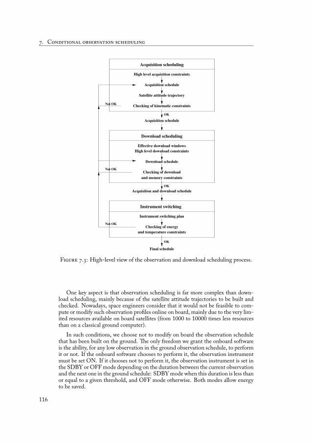
. C
F . : High-level view of the observation and download scheduling process.
One key aspect is that observation scheduling is far more complex than down-load scheduling, mainly because of the satellite attitude trajectories to be built andchecked. Nowadays, space engineers consider that it would not be feasible to com-pute or modify such observation pro les online on board, mainly due to the very lim-ited resources available on board satellites (from 1000 to 10000 times less resourcesthan on a classical ground computer).
In such conditions, we choose not to modify on board the observation schedulethat has been built on the ground. e only freedom we grant the onboard softwareis the ability, for any low observation in the ground observation schedule, to performit or not. If the onboard software chooses to perform it, the observation instrumentmust be set ON. If it chooses not to perform it, the observation instrument is set inthe SDBY or OFF mode depending on the duration between the current observationand the next one in the ground schedule: SDBY mode when this duration is less thanor equal to a given threshold, and OFF mode otherwise. Both modes allow energyto be saved.
116
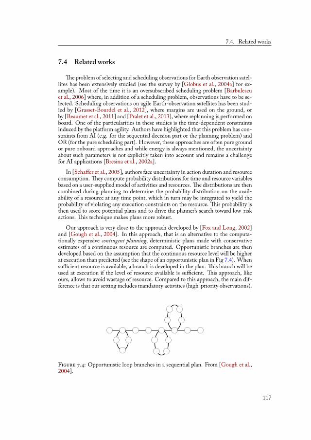
7.4. Related works
7.4 Related works
e problem of selecting and scheduling observations for Earth observation satel-lites has been extensively studied (see the survey by [Globus et al., 2004a] for ex-ample). Most of the time it is an oversubscribed scheduling problem [Barbulescuet al., 2006] where, in addition of a scheduling problem, observations have to be se-lected. Scheduling observations on agile Earth-observation satellites has been stud-ied by [Grasset-Bourdel et al., 2012], where margins are used on the ground, orby [Beaumet et al., 2011] and [Pralet et al., 2013], where replanning is performed onboard. One of the particularities in these studies is the time-dependent constraintsinduced by the platform agility. Authors have highlighted that this problem has con-straints from AI (e.g. for the sequential decision part or the planning problem) andOR (for the pure scheduling part). However, these approaches are often pure groundor pure onboard approaches and while energy is always mentioned, the uncertaintyabout such parameters is not explicitly taken into account and remains a challengefor AI applications [Bresina et al., 2002a].
In [Schaffer et al., 2005], authors face uncertainty in action duration and resourceconsumption. ey compute probability distributions for time and resource variablesbased on a user-supplied model of activities and resources. e distributions are thencombined during planning to determine the probability distribution on the avail-ability of a resource at any time point, which in turn may be integrated to yield theprobability of violating any execution constraints on the resource. is probability isthen used to score potential plans and to drive the planner’s search toward low-riskactions. is technique makes plans more robust.
Our approach is very close to the approach developed by [Fox and Long, 2002]and [Gough et al., 2004]. In this approach, that is an alternative to the computa-tionally expensive contingent planning, deterministic plans made with conservativeestimates of a continuous resource are computed. Opportunistic branches are thendeveloped based on the assumption that the continuous resource level will be higherat execution than predicted (see the shape of an opportunistic plan in Fig 7.4). Whensufficient resource is available, a branch is developed in the plan. is branch will beused at execution if the level of resource available is sufficient. is approach, likeours, allows to avoid wastage of resource. Compared to this approach, the main dif-ference is that our setting includes mandatory activities (high-priority observations).
F . : Opportunistic loop branches in a sequential plan. From [Gough et al.,2004].
117

. C
7.5 Building a conditional observation schedule on the groundHere, we assume that a sequence Seq = [oi, ..., oj ] enforcing agility constraints
has been produced. A conditional observation schedule is a classical observationschedule, that is a sequence Seq of observations, where a required level of energy isassociated with each observation. e required level of energy associated with anobservation i ∈ Seq is the minimum level of energy that is necessary to perform iand all the mandatory activities that follow i, that is all the high-priority observationsthat follow i in Seq and all the future required activities such as downloads. Anexample of conditional schedule is given in Fig. 7.5.
F . : Conditional observation schedule. High-priority observations aremandatory and low-priority observations are executed only if the current onboardlevel of energy E is greater than the required level of energy Ren computed on theground.
Because the download schedule is exible (see previous part), we do not exactlyknow what will be actually downloaded (other than the certainty that high-prioritydownloads will be executed). To overcome this difficulty, we make a pessimisticassumption: all the download windows or at least those used to download high-priority observations will be completely used; hence, the antenna will be maintainedON over these windows and SDBY or OFF between these windows, according to therules presented in Sect.7.3. Of course, when several download windows overlap, weassume that the instrument will be maintained ON only during the window resultingfrom their union.
118
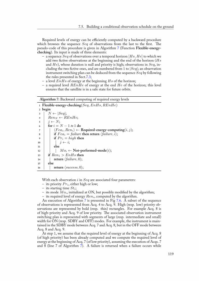
7.5. Building a conditional observation schedule on the ground
Required levels of energy can be efficiently computed by a backward procedurewhich browses the sequence Seq of observations from the last to the rst. epseudo-code of this procedure is given in Algorithm 7 (Function Flexible-energy-checking). Its input is made of three elements:
– a sequence Seq of observations over a temporal horizon [Hs, He] to which weadd two ctive observations at the beginning and the end of the horizon (Hsand He), whose duration is null and priority is high; observations in Seq, in-cluding the two ctive ones, and are numbered from 1 to |Seq|; an observationinstrument switching plan can be deduced from the sequence Seq by followingthe rules presented in Sect.7.3;
– a level EnHs of energy at the beginning Hs of the horizon;– a required level REnHe of energy at the end He of the horizon; this level
ensures that the satellite is in a safe state for future orbits.
Algorithm 7: Backward computing of required energy levels1 Flexible-energy-checking(Seq, EnHs, REnHe)2 begin3 N ← |Seq|;4 RenN ← REnHe;5 j ← N ;6 for i = N − 1 to 1 do7 ⟨F eai, Reni⟩ ← Required-energy-computing(i, j);8 if F eai = failure then return ⟨failure, i⟩;9 if P ri = high then
10 j ← i;11 else12 Moi ← Not-performed-mode(i);13 if Ren1 > EnHs then14 return ⟨failure, 0⟩;15 else16 return ⟨success, 0⟩;
With each observation i in Seq are associated four parameters:– its priority P ri, either high or low;– its starting time Sti;– its mode Moi, initialized at ON, but possibly modi ed by the algorithm;– its required level of energy Reni, computed by the algorithm.An execution of Algorithm 7 is presented in Fig 7.6. A subset of the sequence
of observations is represented from Acq. 4 to Acq. 9. High (resp. low) priority ob-servations are represented by bold (resp. thin) rectangles. For example Acq. 8 isof high-priority and Acq. 9 of low priority. e associated observation instrumentswitching plan is represented with segments of large (resp. intermediate and small)width for ON (resp. SDBY and OFF) modes. For example, the instrument is main-tained in the SDBY mode between Acq. 7 and Acq. 8, but in the OFF mode betweenAcq. 8 and Acq. 9.
At step 1, we assume that the required level of energy at the beginning of Acq. 8(of high priority) has been already computed and we compute the required level ofenergy at the beginning of Acq. 7 (of low priority), assuming the execution of Acqs. 7and 8 (line 7 of Algorithm 7). A failure is returned when a failure occurs while
119
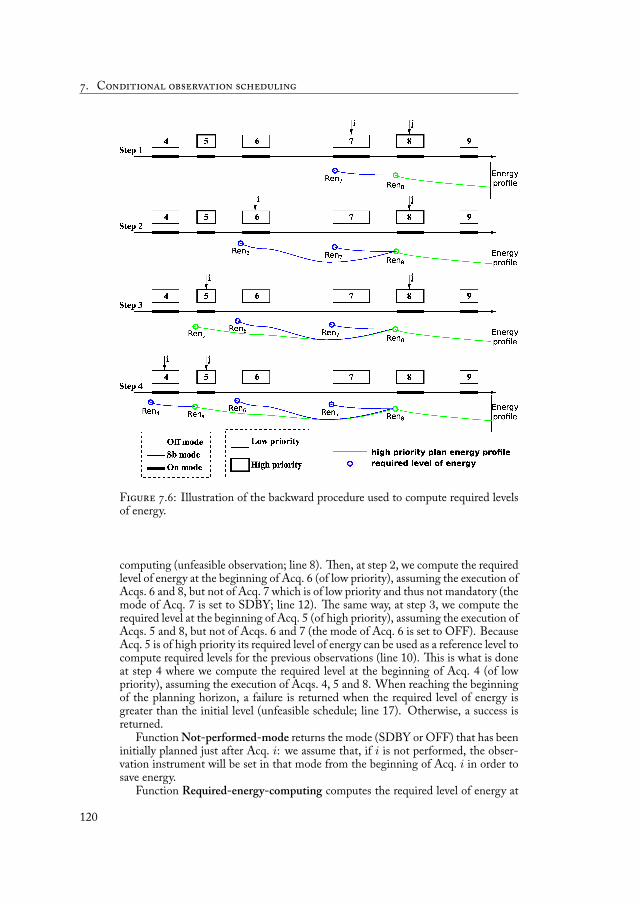
. C
F . : Illustration of the backward procedure used to compute required levelsof energy.
computing (unfeasible observation; line 8). en, at step 2, we compute the requiredlevel of energy at the beginning of Acq. 6 (of low priority), assuming the execution ofAcqs. 6 and 8, but not of Acq. 7 which is of low priority and thus not mandatory (themode of Acq. 7 is set to SDBY; line 12). e same way, at step 3, we compute therequired level at the beginning of Acq. 5 (of high priority), assuming the execution ofAcqs. 5 and 8, but not of Acqs. 6 and 7 (the mode of Acq. 6 is set to OFF). BecauseAcq. 5 is of high priority its required level of energy can be used as a reference level tocompute required levels for the previous observations (line 10). is is what is doneat step 4 where we compute the required level at the beginning of Acq. 4 (of lowpriority), assuming the execution of Acqs. 4, 5 and 8. When reaching the beginningof the planning horizon, a failure is returned when the required level of energy isgreater than the initial level (unfeasible schedule; line 17). Otherwise, a success isreturned.
Function Not-performed-mode returns the mode (SDBY or OFF) that has beeninitially planned just after Acq. i: we assume that, if i is not performed, the obser-vation instrument will be set in that mode from the beginning of Acq. i in order tosave energy.
Function Required-energy-computing computes the required level of energy at
120

7.5. Building a conditional observation schedule on the ground
Algorithm 8: Backward computing of required energy levels1 Required-energy-computing(i, j)2 begin3 ren← Renj ;4 t← Stj ;5 while t > Sti do6 ren← max(Emin, ren− Power(t) ·∆t);7 if ren > Emax then return ⟨failure, ren⟩;8 t← t−∆t;9 return ⟨success, ren⟩;
the beginning of Acq. i assuming that the required level of energy at the beginningof Acq. j (of high priority) has been already computed. Such a computation is per-formed backward step-by-step from the beginning of Acq. j to the beginning ofAcq. i. It is performed step-by-step because the production and consumption of en-ergy are variable. e production depends on the fact that the satellite is in eclipse ornot and, if it is not in eclipse, on the satellite attitude. e consumption depends onthe mode of the instruments (observation instrument and emission antenna) whichmay be ON, SDBY, or OFF. We assume a step of length ∆t, small enough toconsider that energy production and consumption are constant over any interval oflength ∆t.
e pseudo-code of this function is given in Algorithm 8. At each step, therequired level of energy at time t−∆t is computed from the required level of energyat time t already computed. Function Power returns the power produced betweent − ∆t and t (assumed to be constant). is power takes into account the powerproduction of the solar panels Ppsolar(t) and the power consumption Pc(t) of theobservation instrument, of the emission antenna, and of the satellite platform. It isde ned as:
Power(t) = Ppsolar(t)−Pc(t) (7.1)Hence, it may be positive or negative. During day periods, power production
Ppsolar(t) depends on the satellite attitude att(t) at time t and hpAtt(t) the opti-mal attitude where solar panels are directed towards the Sun:
Ppsolar(t) = max(0, Psun · cos(angle(att(t), hpAtt(t)))) (7.2)e forward evolution of the energy level en on board the satellite from t −∆t
to t is given by Eq. 7.3, where we assume that Emin ≤ en(t−∆t) ≤ Emax withEmin and Emax the minimum and maximum energy levels:
en(t) = min(Emax, en(t−∆t) + Power(t) ·∆t) (7.3)
is equation takes into account that the energy level cannot be greater thanEmax. A failure occurs when the energy level is lower than Emin (unacceptablelevel).
From this forward equation, it is possible to deduce an equation which givesthe backward evolution of the required level of energy ren on board the satel-
121

. C
lite from t to t − ∆t. If we assume that Emin ≤ ren(t) ≤ Emax:
ren(t−∆t) = min(e | (min(Emax, e + Power(t) ·∆t)≥ ren(t)) ∧ (e ≥ Emin)
= min(e | (Emax ≥ ren(t))∧(e + Power(t) ·∆t ≥ ren(t))∧(e ≥ Emin)
= min(e | (e ≥ ren(t)− Power(t) ·∆t)∧(e ≥ Emin) (7.4)
= max(Emin, ren(t)− Power(t) ·∆t)
Eq. 7.4 is used at line 6 of Algorithm 8. A failure is returned when the requiredenergy level is greater than Emax (unsatis able requirement; line 7).
7.6 Executing a conditional observation schedule on boardOn board, all high-priority observations are executed. Before each low-priority
observation i, if the current level of energy is greater than or equal to the required levelof energy Reni computed on the ground, observation i is executed. Otherwise theobservation instrument is put into the mode (SDBY or OFF) that has been initiallyplanned just after observation i in order to save energy (see Fig. 7.7 for an example).
F . : Observation cancellation and its effect on energy. On board, there is arequired level of energy for each observation o1, o2, o3, o4, o5. Before a low-priorityobservation such as o3, if the onboard energy level is lower than the required levelcomputed on the ground, the observation is canceled to save energy to ensure thatfuture high-priority observations can still be executed.
As in the exible approach for data download scheduling, we want to ensure thatthe mechanism allows all high-priority observations to be performed. First, at theend of the backward procedure, it is sure that the plan made only of high-priority
122
7.7. Experiments
observations is executable as maximum energy consumptions and minimum energyproduction have been used for this subset of observations. If observation oi at indexi has high-priority, it is sure that all high-priority observations after oi can be done.Now let us consider a low-priority observation oi−1 at index i − 1. e requiredlevel of energy for oi−1 has been computed by going from the required level for oi
and by simulating backward from oi to the start of oi−1. All download windowshave been accounted for. en, if the onboard energy is greater than Reni−1 at thestart of oi−1, it is sure that it is greater than Reni at the start of oi. en all futurehigh-priority observations can be executed.
7.7 ExperimentsIn this section we evaluate the exible observation scheduling mechanism pro-
posed.
7.7.1 Approaches to be comparedTo assess the positive impact of sharing decision-making between ground and
onboard planning for observation scheduling, we implemented and compared thefollowing three approaches into a satellite simulator we developed (details are givenin Appendix A) and already used for experiments on the data download problem:
1. Planning on the ground with coarse energy checking (GroundHiLevel): obser-vation planning is performed on the ground with an algorithm which veri-es high-level constraints limiting the observation duration over each orbit
to indirectly enforce energy constraints. If the schedule is inconsistent withthese constraints, the least valuable observations are removed and the processis started again. On board, the plan is executed without any change. ismethod is close to the currently operational method.
2. Planning on the ground with ne energy checking (GroundFine): observationplanning is performed on the ground with an algorithm which simulates theexecution of the schedule step-by-step with maximum power consumptionand minimum power production for all observations (high and low-priority).During simulation, when the onboard level of energy is strictly lower thanEmin, low-priority observations are removed from the plan and the processis started again. On board, the plan is executed without any change.
3. Conditional planning (Conditional): observation planning is performed onthe ground with an algorithm which computes backward, for all low-priorityobservations, the level of energy that is required to perform it and all the futurehigh-priority observations (see Algorithm 7). During backward computing,if the required level of energy for an observation o is greater than Emax,meaning that more than the maximum level of energy is needed to perform oand the future high-priority observations, observations are removed from theplan and the process is started again. On board, low-priority observations areexecuted if and only if the current level of energy is greater than the requiredlevel computed on the ground.
7.7.2 ScenariosWe used one realistic scenario produced by Airbus Defence and Space. is sce-
nario covers one day. It involves 5 users, 2 priority levels (high and low), 3 ground
123
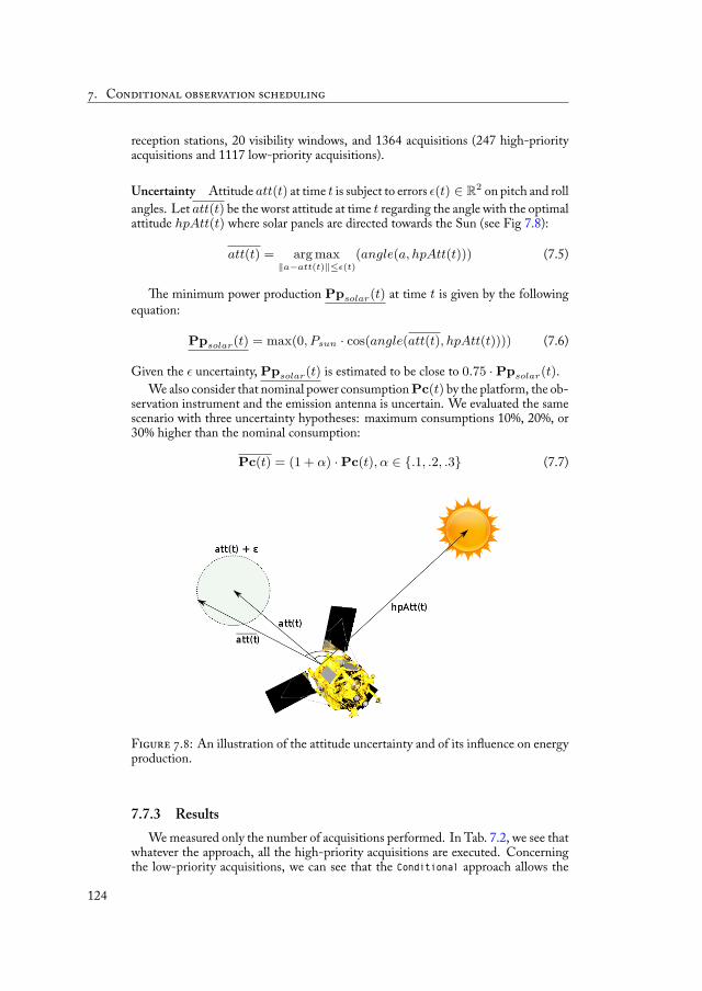
. C
reception stations, 20 visibility windows, and 1364 acquisitions (247 high-priorityacquisitions and 1117 low-priority acquisitions).
Uncertainty Attitude att(t) at time t is subject to errors ϵ(t) ∈ R2 on pitch and rollangles. Let att(t) be the worst attitude at time t regarding the angle with the optimalattitude hpAtt(t) where solar panels are directed towards the Sun (see Fig 7.8):
att(t) = arg max∥a−att(t)∥≤ϵ(t)
(angle(a, hpAtt(t))) (7.5)
e minimum power production Ppsolar(t) at time t is given by the followingequation:
Ppsolar(t) = max(0, Psun · cos(angle(att(t), hpAtt(t)))) (7.6)
Given the ϵ uncertainty, Ppsolar(t) is estimated to be close to 0.75 ·Ppsolar(t).We also consider that nominal power consumption Pc(t) by the platform, the ob-
servation instrument and the emission antenna is uncertain. We evaluated the samescenario with three uncertainty hypotheses: maximum consumptions 10%, 20%, or30% higher than the nominal consumption:
Pc(t) = (1 + α) ·Pc(t), α ∈ .1, .2, .3 (7.7)
F . : An illustration of the attitude uncertainty and of its in uence on energyproduction.
7.7.3 ResultsWe measured only the number of acquisitions performed. In Tab. 7.2, we see that
whatever the approach, all the high-priority acquisitions are executed. Concerningthe low-priority acquisitions, we can see that the Conditional approach allows the
124
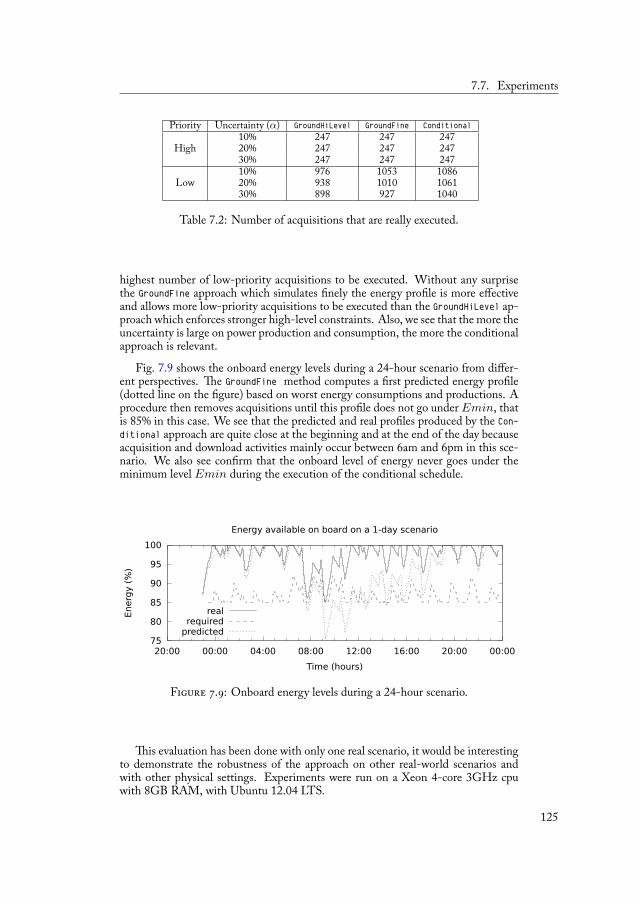
7.7. Experiments
Priority Uncertainty (α) GroundHiLevel GroundFine Conditional
High10% 247 247 24720% 247 247 24730% 247 247 247
Low10% 976 1053 108620% 938 1010 106130% 898 927 1040
Table 7.2: Number of acquisitions that are really executed.
highest number of low-priority acquisitions to be executed. Without any surprisethe GroundFine approach which simulates nely the energy pro le is more effectiveand allows more low-priority acquisitions to be executed than the GroundHiLevel ap-proach which enforces stronger high-level constraints. Also, we see that the more theuncertainty is large on power production and consumption, the more the conditionalapproach is relevant.
Fig. 7.9 shows the onboard energy levels during a 24-hour scenario from differ-ent perspectives. e GroundFine method computes a rst predicted energy pro le(dotted line on the gure) based on worst energy consumptions and productions. Aprocedure then removes acquisitions until this pro le does not go under Emin, thatis 85% in this case. We see that the predicted and real pro les produced by the Con-ditional approach are quite close at the beginning and at the end of the day becauseacquisition and download activities mainly occur between 6am and 6pm in this sce-nario. We also see con rm that the onboard level of energy never goes under theminimum level Emin during the execution of the conditional schedule.
75
80
85
90
95
100
20:00 00:00 04:00 08:00 12:00 16:00 20:00 00:00
Ener
gy (%
)
Time (hours)
Energy available on board on a 1-day scenario
realrequired
predicted
F . : Onboard energy levels during a 24-hour scenario.
is evaluation has been done with only one real scenario, it would be interestingto demonstrate the robustness of the approach on other real-world scenarios andwith other physical settings. Experiments were run on a Xeon 4-core 3GHz cpuwith 8GB RAM, with Ubuntu 12.04 LTS.
125
. C
7.8 Future worksCoupling with the data download planning e acquisition scheduling problem isstrongly connected with the data download problem (see Fig. 7.3). In the exibleapproach, we make the strong assumption that all download windows are used fordownloading. Whereas this is close to reality in over-subscribed scenarios such asdefense scenarios where there are few ground stations and then few visibility win-dows, it is far from true in civil-oriented scenarios where there are a large number ofground stations that cover all continents and are generally underused. is assump-tion makes the acquisition schedule very pessimistic. Work remains to be done to useresults from the download planning phase during the computation of required energylevels. One possibility would be to consider that downloading high-priority acqui-sitions is the only mandatory requirement. In that case, only the visibility windowsneeded for that would be taken into account when simulating the schedule. Fol-lowing the same Conditional approach, required energy levels would be computedon the ground for each group of visibility windows (a group constitutes an onboarddownload planning horizon). On board, before any of these groups, if the actuallevel of energy is sufficient, then the whole group could be used for downloading.Otherwise, only high-priority downloads would be executed to save energy.
Temperature As said, this conditional mechanism can be easily extended to takethe uncertainty about onboard temperature into account. A ne temperature modelis not available on the ground when planning. High-level constraints are then usedduring the planning process. In Tab. 7.1, we see that 9% of the observations are re-jected during the planning phase because of these high-level temperature constraints.
Computing observation pro les on board As already said in a previous chapter,computing observation pro les and more generally attitude trajectories can be mod-eled as a continuous CSP [Beaumet et al., 2007]. Space engineers consider that thecurrent technology does not allow observation pro les to be efficiently computed onboard because of the scarce computing resources. at is why observation schedulingis kept on the ground. Being able to compute these pro les onboard would allow todesign the same kind of mixed decision-making mechanism as in the data downloadproblem (as it has recently been done for the EO-1 satellite [Chien and Troesch,2015]). If onboard computation is not possible, it is still manageable to compute onthe ground conditional observation plans with associated pro les for each branch.
126
Conclusion and perspectives 8
In this manuscript, we have tried to show the possibilities and bene ts of adecision-making mechanism that is shared between ground and onboard for an agileEarth-observation satellite.
After having introduced some preliminaries about decision-making under uncer-tainty, it was observed that the current methods for handling uncertainty in Earth-observation missions was either computing robust low-quality plans on the groundor unpredictable high-quality plans on board. More general methods from combi-natorial optimization were shown and their limitations have been pointed out withregard to our problems.
e main contribution of this thesis is the development of exible decision-making mechanisms. It is inspired by both proactive and reactive methods. Inthis exible approach, differently from pure ground or pure onboard approaches,the available computing power on the ground is used to produce high-quality ro-bust plans together with additional features allowing to quickly adapt plans on boardwhere uncertainty is low. Advantages from both planning phases, offline and online,are being used to balance efficiency and predictability.
Such an approach has been rst applied to tackle the dynamic data downloadproblem with uncertainty about le volumes. is problem has been modeled asa discrete optimization problem. e latter contains some features which are closeother combinatorial problems such as multi-knapsack problems or job-shop schedul-ing problems but it also contains application features which prevented us from di-rectly reusing existing search schemes.
Exact and approximation algorithms have been used to solve the deterministicversion of this data download problem, that is the version without uncertainty. Exactmethods has not seemed scalable to real instances and approximation algorithms havebeen able to produce high-quality solutions.
In the exible decision-making mechanism developed, a metaheuristic builds adownload schedule on the ground as well as bounds on resource consumption forall high-priority observations. is schedule is produced on a deterministic versionof the problem where mean volumes are used for low-priority observations, whichallows to schedule more downloads than in the pure ground approach, and maxi-mum volumes are used for high-priority observations. An onboard chronologicaladaptation mechanism is used (1) to quickly repair the schedules if real volumes oflow-priority observations endanger future high-priority observations, (2) to insertnew observation downloads if possible, (3) to move observation downloads forwardin the schedule if possible. Various algorithms have been implemented into a satellitesimulator and experiments have been conducted to compare this exible mechanismwith its pure ground and pure onboard counterparts. In the end, exible schedul-ing is able to perform as well as pure onboard scheduling on most criteria and tooutperform it on the sharing of the system.
e observation planning problem has been investigated as well and the samedecision-making sharing mechanism has been applied to tackle uncertainty on en-ergy production and energy consumption on board the satellite. However in this case,plans are not adaptable plans but conditional plans containing branches dependinglevel of energy available at execution time. In the same spirit as in the previous prob-lem, the idea is to perform the maximum number of low-priority activities whileensuring that future high-priority activities will be executable with regard to their
127
. C
resource consumption. Experiments have showed that the mixed approach is verypromising against existing approaches.
Perspectives
Future works have been pointed out in previous chapters. We summarize themand point out other more general perspectives.
Data download scheduling problem
– Approximation algorithms such as the SWO scheme are used to compute datadownload schedules. Estimating their efficiency by comparing the quality oftheir solutions to optimal solutions would be interesting. As it seems quite dif-cult to compute optimal solutions for real-life scenarios, there are two options
which are not perfect but satisfying enough to get an idea. A rst option wouldbe to try to compute the distance between optimal and approximate solutionson smaller but sufficiently constrained instances. e second option would in-volve the real scenarios but the approximation algorithms would be comparedwith optimal solutions for the relaxed subproblems only (such as the assign-ment or scheduling subproblems) as there are far easier to solve than whenthey are all integrated.
– We used a very simple model of uncertainty. For now, we assumed that uncer-tainty about le volumes was uniformly distributed over the interval of uncer-tainty. Other models could be evaluated as well as the introduction of a forecastmodel. Such a model would allow ground scheduling to be better informed.
– We could evaluate exible data download with new metrics, more scenarioswith a greater variability of stations and repartition of observations betweenusers. For example, an important issue that has still to be addressed is thedesign of a exibility criterion that would assess the exibility of a ground plan.
– Some algorithms have been proposed to build complete download plans. Onthe ground, an SWO scheme on top of a non-chronological greedy algorithmis used. Other metaheuristics could be used such as genetic algorithms. In thesame spirit, it would be interesting to evaluate the in uence of parameters suchas the duration of the planning horizon. On this point, it is usually good to havea large planning horizon in deterministic cases. In the case of problem withuncertainties, it may be a good idea to balance the size of the planning horizonwith the amount of uncertainties. Indeed, if there are too much uncertainties,the plans become quickly inconsistent at execution.
– One of the temporal phases has not really been investigated yet on board, theexecution phase. During this execution, temporal exibility is provided by theformat of the schedule. An onboard reactive rule could be designed to makedecisions for observations nishing during the planning horizon. For example,if such an observation has lower volume than maximum, the execution may bewaiting for other acquisitions for the next station to be reached. In that case,an onboard reactive decision rule may be able, during execution, to insert newdownloads into the schedule to take advantage of this kind of idle period.
128
Observation scheduling problem– Concerning the observation scheduling problem, extensive computational ex-
periments should be conducted on other scenarios to demonstrate the bene tsof the approach proposed.
– Also, it would be desirable to relax the assumption that all visibility windows areused for downloading. Whereas this is close to reality in over-subscribed sce-narios such as defense scenarios where there are few ground stations and thenfew visibility windows, it is far from true in civil-oriented scenarios where thereare a large number of ground stations that cover all continents and are generallyunderused. is assumption makes the acquisition schedule very pessimistic asthe antenna is assumed to be ON most of the time and then consuming a lotof energy. A better option would be to compute on the ground the energylevel required for using each group of visibility windows. On board, beforeany of these groups, if the actual level of energy is sufficient, then the wholegroup could be used freely for downloading data. Otherwise, only high-prioritydownloads would be executed to save energy.
– Future research could consist in adapting the exact same conditional mecha-nism to take the uncertainty about onboard temperature into account. It wouldallow to relax the high-level constraints used during the ground planning phasethat reject 9% of the observations.
– Finally, a signi cant extension would consist in computing observation pro-les on board. is would allow to make the satellite more autonomous and
to design an even more exible decision-making mechanism such as the ex-ible approach for the data download problem. Since it is not possible to com-pute these pro les onboard for the time being, it would still be manageable tocompute conditional observation plans with a conditional attitude pro le (onepro le for each branch of the schedule built on the ground).
Experimental platformAn interesting perspective, for both the data download problem and the obser-
vation scheduling problem would be, as this is part of early design stage, to ll thegap between theory and practice by performing tests on onboard testbed computers.Implementing the approaches would represent a challenge as it would involve thewhole satellite system. Also, speci c constraints for onboard algorithms would haveto be taken into account with regard to the performance and capabilities of onboardcomputers.
Generic exible decision-makingWe have seen that exible decision-making may be used in problems involving
large horizons and uncertainties on a lot of tasks. When some activities are manda-tory such as high-priority observations or downloads, it is still possible to guaranteetheir realization if it is possible to gather worst-case estimations of their resource con-sumptions (maximum les volumes, maximum energy consumption, minimum en-ergy productions...). Several frameworks already existed for decision-making underuncertainty but they sometimes lack scalability, such as stochastic programming forexample. In this manuscript, we have showed that handling large and complex prob-lems is manageable. One possible direction for future works would be to generalizethe framework we have designed for agile Earth-observing satellites to other prob-
129

. C
lems involving uncertainties. Online stochastic combinatorial optimization proposesthe similar idea of unifying two decision-making phases: online fast decision-makingwith offline methods such as sampling. In our approach, the goal is to focus the com-putational effort with regard to the decision-making phase and to ease the adaptationof plans computed offline. Finally, we address more the resource constraints and theidea of guaranteeing the realization of mandatory activities.
130
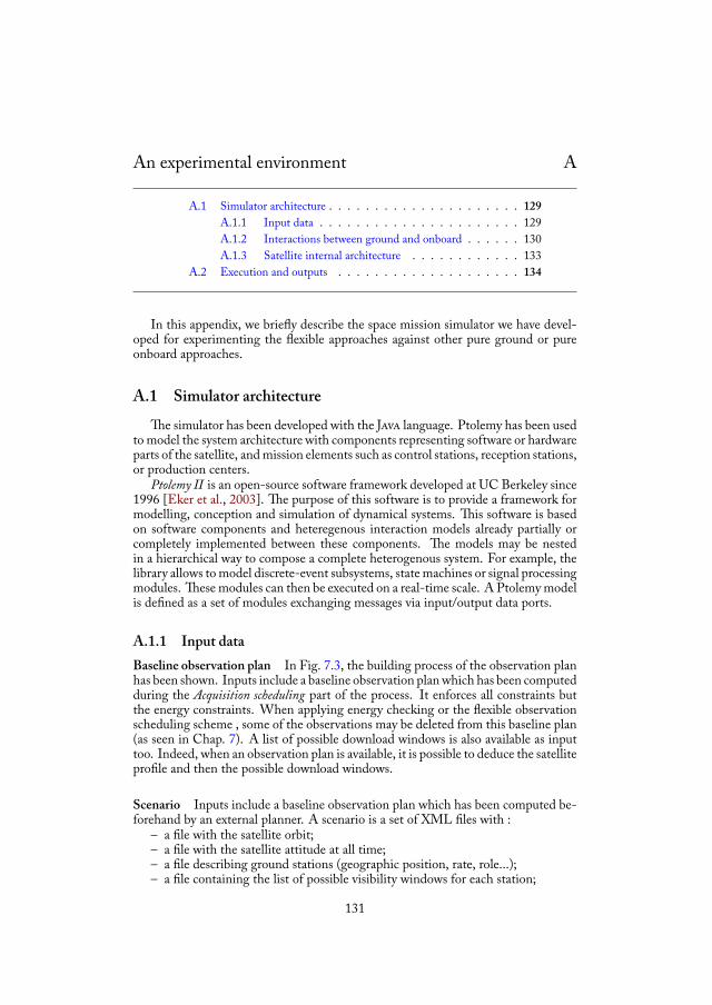
An experimental environment A
A.1 Simulator architecture . . . . . . . . . . . . . . . . . . . . . 129A.1.1 Input data . . . . . . . . . . . . . . . . . . . . . . 129A.1.2 Interactions between ground and onboard . . . . . . 130A.1.3 Satellite internal architecture . . . . . . . . . . . . 133
A.2 Execution and outputs . . . . . . . . . . . . . . . . . . . . 134
In this appendix, we brie y describe the space mission simulator we have devel-oped for experimenting the exible approaches against other pure ground or pureonboard approaches.
A.1 Simulator architecturee simulator has been developed with the J language. Ptolemy has been used
to model the system architecture with components representing software or hardwareparts of the satellite, and mission elements such as control stations, reception stations,or production centers.
Ptolemy II is an open-source software framework developed at UC Berkeley since1996 [Eker et al., 2003]. e purpose of this software is to provide a framework formodelling, conception and simulation of dynamical systems. is software is basedon software components and heteregenous interaction models already partially orcompletely implemented between these components. e models may be nestedin a hierarchical way to compose a complete heterogenous system. For example, thelibrary allows to model discrete-event subsystems, state machines or signal processingmodules. ese modules can then be executed on a real-time scale. A Ptolemy modelis de ned as a set of modules exchanging messages via input/output data ports.
A.1.1 Input dataBaseline observation plan In Fig. 7.3, the building process of the observation planhas been shown. Inputs include a baseline observation plan which has been computedduring the Acquisition scheduling part of the process. It enforces all constraints butthe energy constraints. When applying energy checking or the exible observationscheduling scheme , some of the observations may be deleted from this baseline plan(as seen in Chap. 7). A list of possible download windows is also available as inputtoo. Indeed, when an observation plan is available, it is possible to deduce the satellitepro le and then the possible download windows.
Scenario Inputs include a baseline observation plan which has been computed be-forehand by an external planner. A scenario is a set of XML les with :
– a le with the satellite orbit;– a le with the satellite attitude at all time;– a le describing ground stations (geographic position, rate, role...);– a le containing the list of possible visibility windows for each station;
131

A. A
– a le giving the list of users; for each user, the list of authorized control stationsand reception stations;
– a le containing the acquisition plan initially computed for the scenario.Other mission parameters are generic such as the number of memory banks of
the central memory, the number of download channels, the TMI antenna angularrotation speed, the characteristics of the key table, the maximum number of les thatthe memory can contain... ese parameters are xed according to hypothesis givenby the space agency.
Planning parameters Finally there are several parameters relative to planningwhich specify for example :
– the planning approaches used for data download and observation;– the planning algorithms used on the ground and on board;– the minimum planning horizon on the ground and on board for data download;– the minimum duration required x between the end of the onboard planning
process and the beginning of its execution. By default, this duration is givenby x = 2 · δ/Sa seconds with δ the depointing half-angle and Sa the angularvelocity of the antenna; it then allows to schedule downloads on any stationbecause the antenna will be able to cover any angular distance from its currentposition at the end of the onboard planning process.
A.1.2 Interactions between ground and onboardFig. A.3 shows a simpli ed view of the internal architecture of the simulator for a
scenario with 2 ground reception stations, 2 productions centers, and 1 ground con-trol station. ere is also a Satellite module made of others submodules that we willdetail later. e ground segment is made of one ground reception station module foreach reception station in the scenario, one production center module for each user,control stations and a single mission center. Interactions between ground and on-board are described in Sect. ??. File downloads are represented as communicationsbetween the satellite channels and the ground reception stations. Acknowldegmentsare modeled by messages sent from ground control stations modules to the Down-load module of the satellite. On the ground segment, production centers receive ledownloads from ground reception stations and transmit acknowledgement to controlstations. All theses exchanged messages are delayed with speci c delay generic actorsto represent varying distances and link rates between entities.
e behavior of each actor is de ned in a Java class. It de nes how the actoris processing each message received. It may launch a procedure or send an outputmessage to another module. For example, a production center will send an acknowl-edgement to control stations (to be then sent on board) once it has received all ledownloads for an acquisition. Fig. A.2 shows the Ptolemy networks of connectionsbetween ground actors and satellite actors for an example scenario.
A.1.2.1 Decison-making on the groundOn the ground, decision-making for pure ground or exible scheduling is per-
formed in the Mission center module. For data download scheduling, algorithmspresented in earlier chapters are implemented on top of a constraint-based modelof the data download problem (see Fig. A.3). e library we use for modelling andchecking constraints is presented below.
132

A.1. Simulator architecture
F A. : Schematic view of the simulator.
InCELL Invariant-based Constraint EvaLuation Library or InCELL isconstraint-based local search library developed at ONERA [Pralet and Verfaillie,2013c] that we use in the ground planning system.
InCELL allows to process dynamic problems by using only static models, whichdo not change over the mission horizon. Software embeddedment operational con-straints motivates the use of static models. Avoiding dynamic generation of modelsallows to know beforehand the memory capacity required for planning. It also guar-antees, that there will not be any memory leaks, any memory over ow or wasted timefor model generation.
e library is built upon local search techniques. e latter allows to quicklybuild good quality solutions, using a low amount of memory. Generic techniquesof constraint-based local search, implemented in tools such as COMET [Michel andVan Hentenryck, 2005] and LocalSolver [Benoist et al., 2011]. e basic element
133
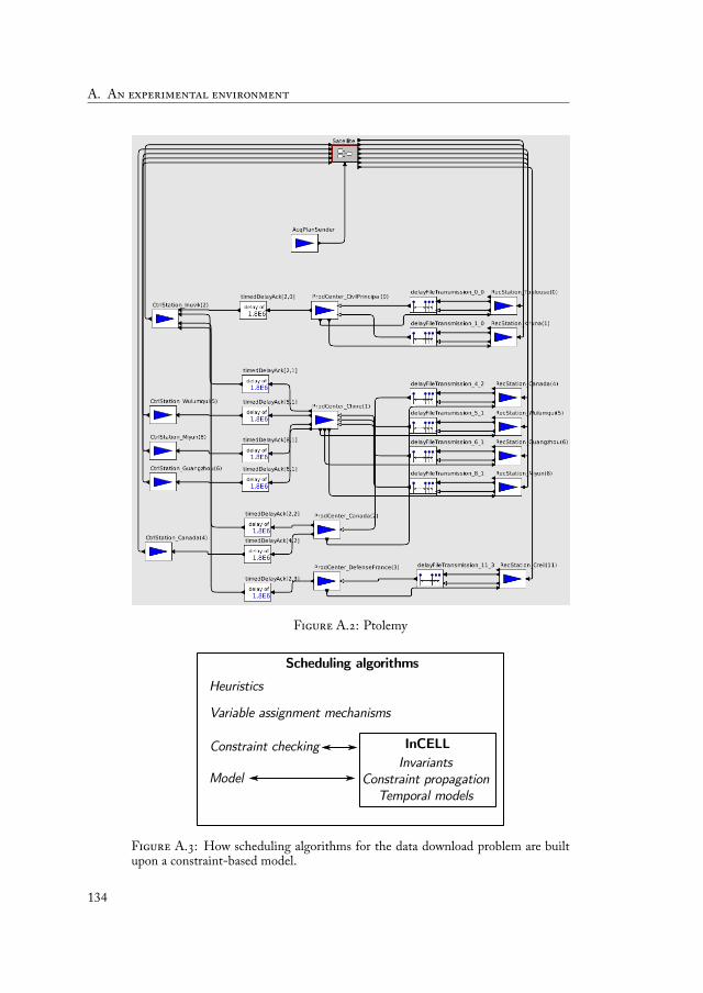
A. A
F A. : Ptolemy
F A. : How scheduling algorithms for the data download problem are builtupon a constraint-based model.
134

A.1. Simulator architecture
handled in these tools is the invariant. Invariants allows to model combinatory con-straints, temporal constraints, resource constraints, and optimization criterions. eypermit to quickly evaluate these values from a model assignement and to incremen-tally reevaluate them when a change is made to the model. e library also includestechniques to manage Simple Temporal Networks [Dechter et al., 1991] and Time-dependant STN [Pralet and Verfaillie, 2013b].
Invariants are the heart of constraint-based local search. In the COMETtool [Michel and Van Hentenryck, 2005], an invariant is de ned as a unidirectionnalconstraint x← exp with x a variable and exp a functional expression of other vari-ables of the problem, for example x← sum(i ∈ [1..N ]) yi. Invariants are automat-ically and incrementally maintained through local search movements. Incrementalevaluation decreases the amount of work required to recompute output values (leftpart of the equation) of invariants following local modi cations in the assignementsof variables contained in the input values (right part of the equation). In the previousexample, if yk changes for k ∈ [1..N ], it is not needed to recompute x from scratch,it simply has to increment x with the difference between the old value of yk and itsnew value. e only requirement to allow incremental reevaluation is that invariantsmust be acyclic, so that a variable is not a function of itself.
In constraint-based local search, the main challenge consists in reevaluating in-variants quickly enough to allow many moves to be done. For that, the evaluationprocess maintains a priority list made of invariants to reevaluate. is list is orderedaccording the topological position of invariants in the directed acyclic graph of invari-ants, which allows to reevaluate invariants no more than once. e list of invariantsto reevaluate initially contains all successors of modi ed root variables. When aninvariant is reevaluated, all successors are added to the priority list (if they were notin it already). e reevaluation process is stopped as soon as the priority list is empty.
F A. : Set of invariants and associated DAG (ite(b; x; y) stands for “if b thenx else y”). From [Pralet and Verfaillie, 2013c].
A.1.3 Satellite internal architecturee Satellite module is said to be composite because it is made of several low-level
modules. Two main modules, Download and Observation, handle onboard decision-making (when applicable) and action execution . ey have a deliberative-reactivebehavior [Lemaître and Verfaillie, 2007]. In this kind of behavior, two distinct ele-ments may be distinguished (see Fig. A.5):
– A deliberative submodule, which is called periodically or following an event.For the Download module, it is activated before each group of sufficiently closedownload windows. is submodule builds a temporally exible plan from aexible plan as de ned in Sect. 6.4.2. It then lls the key change table which
135
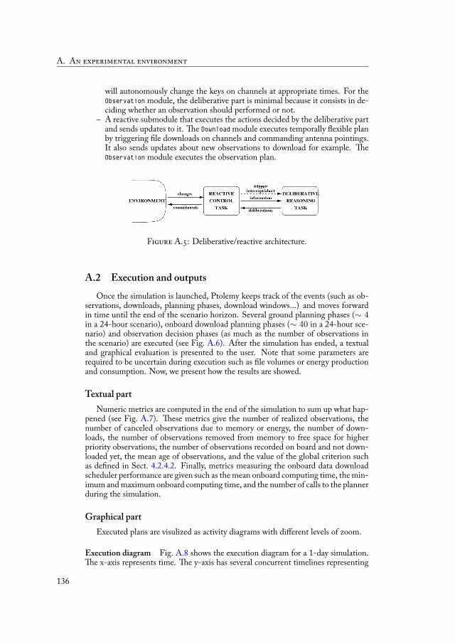
A. A
will autonomously change the keys on channels at appropriate times. For theObservation module, the deliberative part is minimal because it consists in de-ciding whether an observation should performed or not.
– A reactive submodule that executes the actions decided by the deliberative partand sends updates to it. e Download module executes temporally exible planby triggering le downloads on channels and commanding antenna pointings.It also sends updates about new observations to download for example. eObservation module executes the observation plan.
F A. : Deliberative/reactive architecture.
A.2 Execution and outputsOnce the simulation is launched, Ptolemy keeps track of the events (such as ob-
servations, downloads, planning phases, download windows...) and moves forwardin time until the end of the scenario horizon. Several ground planning phases (∼ 4in a 24-hour scenario), onboard download planning phases (∼ 40 in a 24-hour sce-nario) and observation decision phases (as much as the number of observations inthe scenario) are executed (see Fig. A.6). After the simulation has ended, a textualand graphical evaluation is presented to the user. Note that some parameters arerequired to be uncertain during execution such as le volumes or energy productionand consumption. Now, we present how the results are showed.
Textual partNumeric metrics are computed in the end of the simulation to sum up what hap-
pened (see Fig. A.7). ese metrics give the number of realized observations, thenumber of canceled observations due to memory or energy, the number of down-loads, the number of observations removed from memory to free space for higherpriority observations, the number of observations recorded on board and not down-loaded yet, the mean age of observations, and the value of the global criterion suchas de ned in Sect. 4.2.4.2. Finally, metrics measuring the onboard data downloadscheduler performance are given such as the mean onboard computing time, the min-imum and maximum onboard computing time, and the number of calls to the plannerduring the simulation.
Graphical partExecuted plans are visulized as activity diagrams with different levels of zoom.
Execution diagram Fig. A.8 shows the execution diagram for a 1-day simulation.e x-axis represents time. e y-axis has several concurrent timelines representing
136

A.2. Execution and outputs
F A. : Data download planning horizons during simulation. On the top part,the onboard data download planning horizon for a rst set of download windows canbe seen. On the bottom part, the same for the next set of download windows.
download channels (CH_0, ..., CH_4), instrument switching (TELESCOPE, ANTENNA),planning phases (GRDPLAN, BDPLAN), download windows (in green with Vis(Toulouse)for example), and effective communication windows (in red with Dl(Toulouse) forexample).
Fig. A.9 shows a zoomed version of the previous diagram where we can see moreclearly le downloads on channels. Each color is associated with an observation.Observation cancellations due to energy can be seen on the Telescope timeline as itis put into SDBY mode (in yellow).
An activity report is also given as a CSV le. It contains details about the statusof each observation such as its state (done, downloaded, recorded...), its real volumeafter random drawing, or other useful data.
Energy diagram Fig. A.10 shows the real onboard energy pro le (in black) in per-centage of the battery usage. e minimum level of energy to be available onboardis here set to 80%. Concerning the exible observation scheduling approach, it alsoshows the simulated energy pro le when taking into account worst-case energy con-sumptions (in green) and the minimum required level of energy computed for en-suring at each instant that the future high-priority observations will be possible (inblue).
Memory diagram Fig. A.11 shows the memory consumption pro le for one mem-ory bank. is pro le shows the global usage (in black) and the usage per prioritylevel (in red for high-priority observations, in blue for low-priority observations).
137
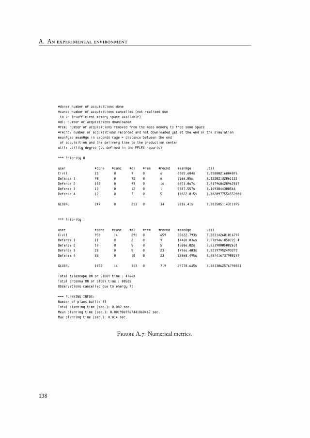
A. A
#done: number of acquisitions done#canc: number of acquisitions cancelled (not realized dueto an insufficient memory space available)
#dl: number of acquisitions downloaded#rem: number of acquisitions removed from the mass memory to free some space#recnd: number of acquisitions recorded and not downloaded yet at the end of the simulationmeanAge: meanAge in seconds (age = distance between the endof acquisition and the delivery time to the production center
util: utility degree (as defined in the PFLEX reports)
*** Priority 0
user #done #canc #dl #rem #recnd meanAge utilCivil 15 0 9 0 6 6565.684s 0.05000216804076Defense 1 98 0 92 0 6 7266.85s 0.12202132861121Defense 2 109 0 93 0 16 6651.067s 0.017968428962817Defense 3 13 0 12 0 1 5987.557s 0.1693844300566Defense 4 12 0 7 0 5 10922.015s 0.0020977554552008
GLOBAL 247 0 213 0 34 7016.41s 0.003585114311875
*** Priority 1
user #done #canc #dl #rem #recnd meanAge utilCivil 950 14 291 0 659 30622.793s 0.003142601016797Defense 1 11 0 2 0 9 14468.036s 7.678946105072E-4Defense 2 10 0 5 0 5 15006.02s 0.03398805082631Defense 3 28 0 5 0 23 14966.403s 0.02197952493272Defense 4 33 0 10 0 23 23068.495s 0.007416737908159
GLOBAL 1032 14 313 0 719 29778.645s 0.0013062576790861
Total telescope ON or STDBY time : 4766sTotal antenna ON or STDBY time : 8052sObservations cancelled due to energy 71
=== PLANNING INFOS:Number of plans built: 43Total planning time (sec.): 0.082 sec.Mean planning time (sec.): 0.0019069767441860467 sec.Max planning time (sec.): 0.014 sec.
F A. : Numerical metrics.
138

A.2. Execution and outputs
F A. : Execution diagram (no zoom) during a 1-day simulation.
F A. : Execution diagram (zoom on a group of activities) during a 1-day sim-ulation.
139
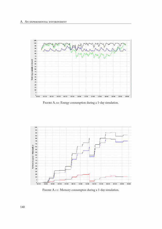
A. A
F A. : Energy consumption during a 1-day simulation.
F A. : Memory consumpton during a 1-day simulation.
140
Guarantees for the R1 insertion rule B
B.1 Schedule Density . . . . . . . . . . . . . . . . . . . . . . . 139B.2 Batch Insertion . . . . . . . . . . . . . . . . . . . . . . . . 140
In this appendix, we provide two guarantees concerning the R1 insertion rulewhich can be seen in Algorithm 3 in Sect. 5.2.1. is procedure is here decomposedinto two other procedures : the E B algorithm which is a generaliza-tion of the R1 insertion algorithm as no heuristic is used for choosing the next leto schedule and the E procedure which schedules one le. First we provethat enqueuing a le with algorithm E returns a schedule without resourcecon ict. Second, we prove that by using iteratively E to schedule all lesof an observation, E B (and then the R1 insertion algorithm) produceschedules that are somewhat balanced on every channels. is work is extracted froma journal paper submitted to Discrete Applied Mathematics [Hebrard et al., 2015].
In this appendix, we use vocabulary from the scheduling literature. Jobs representles and a batch is a set of les linked to an acquisition, resources correspond to
memory banks and parallel machines to telecommunication channels.Also, we use the following notations and conventions:
n: the number of jobs, denoted a1, . . . , an
res(a): the resource required by job apa: the size of job a, whereas pmin and pmax stand for the
minimum and maximum job sizes, respectivelysa and ea: the start and end time of job a in the schedule, respec-
tivelym: the number of machines, denoted M1, . . . , Mm
eM : the end time of the last job scheduled on machine Memin and emax: the completion time of the last job on the ma-
chine nishing rst and last, respectively. at is,emin = min(eMj | 1 ≤ j ≤ m) and emax =max(eMj | 1 ≤ j ≤ m)
λ: the number of resources, denoted R1, . . . , Rλ; More-over, we also use the symbol R to denote the set of jobsrequiring this resource and L(R) stands for the load ofthis resource, that is, the total processing time of its jobs:L(R) =
∑a∈R
pa
B.1 Schedule DensityWe consider a greedy heuristic which iteratively inserts a job a into a partial sched-
ule S. We can de ne an heuristic as an ordering on the jobs and an insertion proce-dure called E and shown in Algorithm 9.
e algorithm E considers a job a and a partial schedule S. We shall seethat there is at most one machine whose last job requires the same resource as a. ejob a is inserted at the back of such machine if it exists, and at the back of the rstavailable machine otherwise.
141
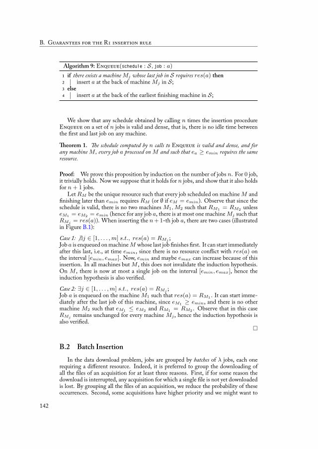
B. G R
Algorithm 9: E (schedule : S, job : a)1 if there exists a machine Mj whose last job in S requires res(a) then2 insert a at the back of machine Mj in S;3 else4 insert a at the back of the earliest nishing machine in S;
We show that any schedule obtained by calling n times the insertion procedureE on a set of n jobs is valid and dense, that is, there is no idle time betweenthe rst and last job on any machine.
eorem 1. e schedule computed by n calls to E is valid and dense, and forany machine M , every job a processed on M and such that ea ≥ emin requires the sameresource.
Proof: We prove this proposition by induction on the number of jobs n. For 0 job,it trivially holds. Now we suppose that it holds for n jobs, and show that it also holdsfor n + 1 jobs.
Let RM be the unique resource such that every job scheduled on machine M andnishing later than emin requires RM (or ∅ if eM = emin). Observe that since the
schedule is valid, there is no two machines M1, M2 such that RM1 = RM2 unlesseM1 = eM2 = emin (hence for any job a, there is at most one machine Mj such thatRMj = res(a)). When inserting the n + 1-th job a, there are two cases (illustratedin Figure B.1):
Case 1: ∃j ∈ [1, . . . , m] s.t., res(a) = RMj ;Job a is enqueued on machine M whose last job nishes rst. It can start immediatelyafter this last, i.e., at time emin, since there is no resource con ict with res(a) onthe interval [emin, emax]. Now, emin and maybe emax can increase because of thisinsertion. In all machines but M , this does not invalidate the induction hypothesis.On M , there is now at most a single job on the interval [emin, emax], hence theinduction hypothesis is also veri ed.
Case 2: ∃j ∈ [1, . . . , m] s.t., res(a) = RMj ;Job a is enqueued on the machine M1 such that res(a) = RM1 . It can start imme-diately after the last job of this machine, since eM1 ≥ emin, and there is no othermachine M2 such that eM1 ≤ eM2 and RM1 = RM2 . Observe that in this caseRMj remains unchanged for every machine Mj , hence the induction hypothesis isalso veri ed.
B.2 Batch InsertionIn the data download problem, jobs are grouped by batches of λ jobs, each one
requiring a different resource. Indeed, it is preferred to group the downloading ofall the les of an acquisition for at least three reasons. First, if for some reason thedownload is interrupted, any acquisition for which a single le is not yet downloadedis lost. By grouping all the les of an acquisition, we reduce the probability of theseoccurrences. Second, some acquisitions have higher priority and we might want to
142
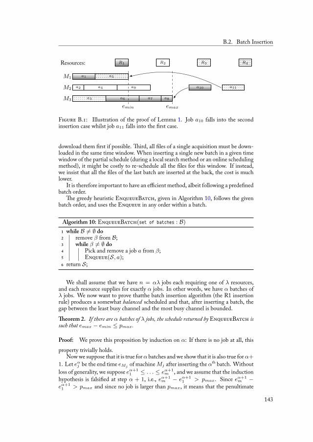
B.2. Batch Insertion
Resources: R1 R2 R3 R4
M1 a1 a5
M2 a2 a4 a9
M3 a3 a6 a7 a8
emin emax
a10 a11
F B. : Illustration of the proof of Lemma 1. Job a10 falls into the secondinsertion case whilst job a11 falls into the rst case.
download them rst if possible. ird, all les of a single acquisition must be down-loaded in the same time window. When inserting a single new batch in a given timewindow of the partial schedule (during a local search method or an online schedulingmethod), it might be costly to re-schedule all the les for this window. If instead,we insist that all the les of the last batch are inserted at the back, the cost is muchlower.
It is therefore important to have an efficient method, albeit following a prede nedbatch order.
e greedy heuristic E B , given in Algorithm 10, follows the givenbatch order, and uses the E in any order within a batch.
Algorithm 10: E B (set of batches : B)1 while B = ∅ do2 remove β from B;3 while β = ∅ do4 Pick and remove a job a from β;5 E (S, a);6 return S;
We shall assume that we have n = αλ jobs each requiring one of λ resources,and each resource supplies for exactly α jobs. In other words, we have α batches ofλ jobs. We now want to prove thatthe batch insertion algorithm (the R1 insertionrule) produces a somewhat balanced scheduled and that, after inserting a batch, thegap between the least busy channel and the most busy channel is bounded.
eorem 2. If there are α batches of λ jobs, the schedule returned by E B issuch that emax − emin ≤ pmax.
Proof: We prove this proposition by induction on α: If there is no job at all, thisproperty trivially holds.
Now we suppose that it is true for α batches and we show that it is also true for α+1. Let eα
j be the end time eMj of machine Mj after inserting the αth batch. Withoutloss of generality, we suppose eα+1
1 ≤ . . . ≤ eα+1m , and we assume that the induction
hypothesis is falsi ed at step α + 1, i.e., eα+1m − eα+1
1 > pmax. Since eα+1m −
eα+11 > pmax and since no job is larger than pmax, it means that the penultimate
143
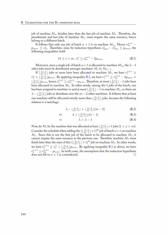
B. G R
job of machine Mm nishes later than the last job of machine M1. erefore, thepenultimate and last jobs of machine Mm must require the same resource, hencebelong to a different batch.
It follows that only one job of batch α + 1 is on machine Mm. Hence eα+1m −
pmax ≤ eαm. erefore, since by induction hypothesis eα
max − eαmin ≤ pmax, the
following inequalities hold:
∀1 ≤ i < m, eαi ≥ eα+1
m − 2pmax (B.1)
Moreover, since a single job of batch α+1 is allocated to machine Mm, the λ−1other jobs must be distributed amongst machines M1 to Mm−1.
If ⌊ λ−1m−1⌋ jobs or more have been allocated to machine M1, we have eα+1
1 ≥eα
1 + ⌊ λ−1m−1⌋pmin. By applying inequality B.1, we have eα+1
1 ≥ eα+1m − 2pmax +
⌊ λ−1m−1⌋pmin, hence eα+1
1 ≥ eα+1m −pmax. erefore, at most ⌊ λ−1
m−1⌋−1 jobs havebeen allocated to machine M1. In other words, among the λ jobs of the batch, onehas been assigned to machine m and at most ⌊ λ−1
m−1⌋−1 to machine M1, so there areλ−⌊ λ−1
m−1⌋ jobs to distribute over the m− 2 other machines. It follows that at leastone machine will be allocated strictly more than ⌊ λ−1
m−1⌋ jobs, because the followingrelation is a tautology:
λ− ⌊ λ−1m−1⌋ > ⌊ λ−1
m−1⌋(m− 2) (B.2)⇔ λ > ⌊ λ−1
m−1⌋(m− 1) (B.3)⇐ λ > λ− 1 (B.4)
Now, let Mj be the machine that was allocated at least ⌊ λ−1m−1⌋+1 jobs (1 < j < m).
Consider the schedule when adding the (⌊ λ−1m−1⌋+1)th job of batch α+1 on machine
Mj . Since this is not the rst job of the batch to be allocated to machine Mj , itcannot require the same resource as the previous one. erefore machine M1 mustnish later than the start of this (⌊ λ−1
m−1⌋+ 1)th job on machine Mj . In other words,we have eα+1
1 ≥ eαj + ⌊ λ−1
m−1⌋pmin. By applying inequality B.1 as above, we haveeα+1
1 ≥ eα+1m − pmax. In both cases, the assumption that the induction hypothesis
does not lift to α + 1 is contradicted.
144

OPL model of the data download problem C
1 using CP;2
3 / *number of channels * /4 i n t Nc = . . . ;5 a s se r t Nc > 0 ;6 / * channels * /7 range Ncs = 1 . .Nc ;8
9 / *number of windows* /10 i n t Nw = . . . ;11 a s se r t Nw > 0 ;12 / *windows* /13 range Nws = 1 . .Nw ;14
15 / * Acquis i t ions * /16 i n t Na = . . . ;17 a s se r t Na > 0 ;18 range Nas = 1 . .Na ;19
20 / *Number of f i l e s * /21 i n t Nf = . . . ;22 / * F i l e s * /23 range Nfs = 1 . .Nf ;24
25 / *number of ground s t a t i on s * /26 i n t Nst = . . . ;27 a s se r t Nst > 0 ;28 / * S ta t ions * /29 range S t s = 1 . . Nst ;30 range Stz = 0 . . Nst ;31
32 / *Number of memory blocks * /33 i n t Nmb = . . . ;34 a s se r t Nmb > 0;35 range Nmbs = 1 . .Nmb;36
37 / *number of e n t i t i e s * /38 i n t Ne = . . . ;39 a s se r t Ne > 0 ;40 / * E n t i t i e s * /41 range Es = 1 . .Ne ;42
43 / *number of p r i o r i t y leve l s * /44 i n t Np = . . . ;45 a s se r t Np > 0 ;46 / * P r i o r i t é s * /
145
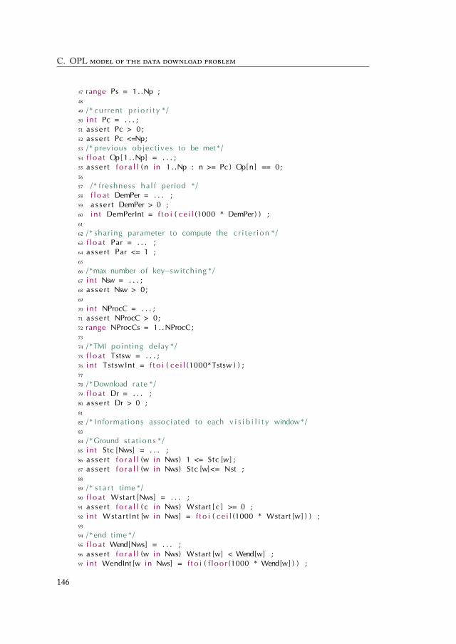
C. OPL
47 range Ps = 1 . .Np ;48
49 / * current p r i o r i t y * /50 i n t Pc = . . . ;51 a s se r t Pc > 0;52 a s se r t Pc <=Np;53 / * previous object ives to be met * /54 f l o a t Op[ 1 . .Np] = . . . ;55 a s se r t f o r a l l ( n in 1 . .Np : n >= Pc ) Op[n] == 0;56
57 / * f reshness ha l f period * /58 f l o a t DemPer = . . . ;59 as se r t DemPer > 0 ;60 i n t DemPerInt = f t o i ( ce i l (1000 * DemPer ) ) ;61
62 / * sharing parameter to compute the c r i t e r i on * /63 f l o a t Par = . . . ;64 a s se r t Par <= 1 ;65
66 / *max number of key−switching * /67 i n t Nsw = . . . ;68 a s se r t Nsw > 0;69
70 i n t NProcC = . . . ;71 a s se r t NProcC > 0;72 range NProcCs = 1 . .NProcC;73
74 / *TMI pointing delay * /75 f l o a t Tstsw = . . . ;76 i n t Ts tswInt = f t o i ( ce i l (1000*Tstsw ) ) ;77
78 / *Download ra te * /79 f l o a t Dr = . . . ;80 a s se r t Dr > 0 ;81
82 / * Informations associated to each v i s i b i l i t y window* /83
84 / *Ground s t a t i on s * /85 i n t Stc [Nws] = . . . ;86 a s se r t f o r a l l (w in Nws) 1 <= Stc [w] ;87 a s se r t f o r a l l (w in Nws) Stc [w]<= Nst ;88
89 / * s t a r t time * /90 f l o a t Wstart [Nws] = . . . ;91 a s se r t f o r a l l ( c in Nws) Wstart [ c ] >= 0 ;92 i n t Wstar t In t [w in Nws] = f t o i ( ce i l (1000 * Wstart [w] ) ) ;93
94 / * end time * /95 f l o a t Wend[Nws] = . . . ;96 a s se r t f o r a l l (w in Nws) Wstart [w] < Wend[w] ;97 i n t WendInt [w in Nws] = f t o i ( f l oo r (1000 * Wend[w] ) ) ;
146

98
99 / * compute the overa l l horizon * /100 f l o a t WstartMin = min (w in Nws) Wstart [w] ;101 f l o a t WendMax = max(w in Nws) Wend[w] ;102 i n t WstartMinInt = min (w in Nws) Wstar t In t [w] ;103 i n t WendMaxInt = max(w in Nws) WendInt [w] ;104
105 / * Informations associated to each acquis i t ion * /106 / * s t a r t time * /107 f l o a t As ta r t [Nas] = . . . ;108 a s se r t f o r a l l ( a in Nas ) As ta r t [ a ] >= 0 ;109 / * end time * /110 f l o a t Astop [Nas] = . . . ;111 i n t AstopInt [ a in Nas] = f t o i ( ce i l (1000 * Astop [a ] ) ) ;112
113 f l o a t Adeadline [Nas] = . . . ;114 a s se r t f o r a l l ( a in Nas ) Adeadline [ a ] >= 0 ;115 i n t AdeadlineInt [ a in Nas] = f t o i ( ce i l (1000 * Adeadline [ a ] ) ) ;116
117 / * p r i o r i t y * /118 i n t Pa [Nas] = . . . ;119 a s se r t f o r a l l ( a in Nas ) 1 <= Pa[a ] ;120 a s se r t f o r a l l ( a in Nas ) Pa [ a ] <= Np ;121
122 / * normalised weight * /123 f l o a t Wn[Nas] = . . . ;124 a s se r t f o r a l l ( a in Nas ) Wn[a ] > 0 ;125 f l o a t Wnmin = min ( a in Nas ) Wn[a ] ;126 f l o a t Umin = 0.0000001;127
128 / * associated en t i t y * /129 i n t Ea [Nas] = . . . ;130 a s se r t f o r a l l ( a in Nas ) Ea [ a ] <= Ne ;131 a s se r t f o r a l l ( a in Nas ) 1 <= Ea [a ] ;132
133 / * Informations fo r each f i l e * /134
135 / *memory block * /136 i n t Mb[Nfs ] = . . . ;137 a s se r t f o r a l l ( f in Nfs ) Mb[ f ] >= 1 ;138 a s se r t f o r a l l ( f in Nfs ) Mb[ f ] <= Nmb ;139
140 / * corresponding acquis i t ion * /141 i n t Acqf [Nfs ] = . . . ;142
143 / * encrypting key * /144 i n t Kf [Nfs ] = . . . ;145
146 / * generated volume* /147 f l o a t V[Nfs ] = . . . ;148 a s se r t f o r a l l ( f in Nfs ) V[ f ] >= 0 ;
147
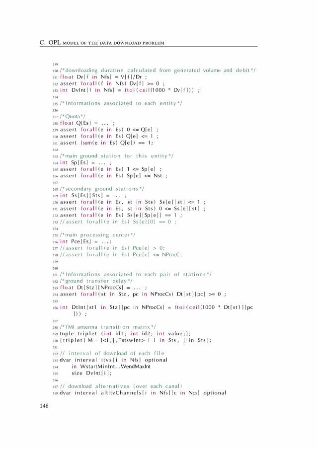
C. OPL
149
150 / * downloading duration calculated from generated volume and debit * /151 f l o a t Dv[ f in Nfs ] = V[ f ] / Dr ;152 a s se r t f o r a l l ( f in Nfs ) Dv[ f ] >= 0 ;153 i n t DvInt [ f in Nfs ] = f t o i ( ce i l (1000 * Dv[ f ] ) ) ;154
155 / * Informations associated to each en t i t y * /156
157 / *Quota * /158 f l o a t Q[ Es ] = . . . ;159 a s se r t f o r a l l ( e in Es ) 0 <= Q[e ] ;160 a s se r t f o r a l l ( e in Es ) Q[e ] <= 1 ;161 a s se r t ( sum( e in Es ) Q[e ] ) == 1;162
163 / *main ground s ta t ion fo r t h i s en t i t y * /164 i n t Sp [ Es ] = . . . ;165 a s se r t f o r a l l ( e in Es ) 1 <= Sp[e ] ;166 a s se r t f o r a l l ( e in Es ) Sp [e ] <= Nst ;167
168 / * secondary ground s t a t i on s * /169 i n t Ss [ Es ] [ S t s ] = . . . ;170 a s se r t f o r a l l ( e in Es , s t in S t s ) Ss [ e ] [ s t ] <= 1 ;171 a s se r t f o r a l l ( e in Es , s t in S t s ) 0 <= Ss [ e ] [ s t ] ;172 a s se r t f o r a l l ( e in Es ) Ss [ e ] [ Sp [e ] ] == 1 ;173 / / a s s e r t f o r a l l ( e in Es ) Ss [ e ] [0 ] == 0 ;174
175 / *main processing center * /176 i n t Pce [ Es ] = . . . ;177 / / a s s e r t f o r a l l ( e in Es ) Pce [ e ] > 0;178 / / a s s e r t f o r a l l ( e in Es ) Pce [ e ] <= NProcC;179
180
181 / * Informations associated to each pair of s t a t i on s * /182 / * ground t r an s f e r delay * /183 f l o a t Dt [ Stz ] [NProcCs ] = . . . ;184 a s se r t f o r a l l ( s t in Stz , pc in NProcCs ) Dt [ s t ] [ pc ] >= 0 ;185
186 i n t DtInt [ s t1 in Stz ] [ pc in NProcCs ] = f t o i ( ce i l (1000 * Dt [ s t1 ] [ pc] ) ) ;
187
188 / *TMI antenna t r an s i t i on matrix * /189 tuple t r i p l e t i n t id1 ; i n t id2 ; i n t value ; ;190 t r i p l e t M = < i , j , TstswInt > | i in Sts , j in S t s ;191
192 / / i n t e r va l of download of each f i l e193 dvar in t e r va l i t v s [ i in Nfs ] optional194 in WstartMinInt . .WendMaxInt195 s ize DvInt [ i ] ;196
197 / / download a l t e rna t i ve s ( over each canal )198 dvar in t e r va l a l t I tvChannels [ i in Nfs ] [ c in Ncs] optional
148

199 in WstartMinInt . .WendMaxInt200 s ize DvInt [ i ] ;201
202 / / download a l t e rna t i ve s ( over each window)203 dvar in t e r va l altItvWindows [ i in Nfs ] [w in Nws] optional204 in Wstar t In t [w] . . WendInt [w]205 s ize DvInt [ i ] ;206
207 / / sequence of downloads fo r each canal208 dvar sequence dlseq [c in Ncs] in209 a l l ( i in Nfs ) a l t I tvChannels [ i ] [ c ] types210 a l l ( i in Nfs ) Kf [ i ] ;211
212 / * span of a l l downloads fo r each window * /213 dvar in t e r va l spanOverWindows[w in Nws] optional214 in Wstar t In t [w] . . WendInt [w]215 s ize 0 . .WendInt [w] − Wstar t In t [w] ;216
217 / / sequence of windows218 dvar sequence dlseqw in219 a l l (w in Nws) spanOverWindows[w] types220 a l l (w in Nws) Stc [w] ;221
222 / / key associated with the download preceding the download of af i l e on the same canal
223 dexpr i n t keyPrev [ i in Nfs ] = max( c in Ncs ) typeOfPrev ( dlseq [c ] ,a l t I tvChannels [ i ] [ c ] ,0 ) ;
224
225 dexpr i n t nChangeKeys = sum( f in Nfs ) ( keyPrev [ f ] != 0 && keyPrev [ f] != Kf [ f ] ) ;
226
227 dexpr i n t acqdl [ i in Nas] = max( f in Nfs : Acqf [ f ] == i ) presenceOf( i t v s [ f ] ) ;
228
229 / / s t a t i on where a i s downloaded230 dexpr i n t d lS ta t ion [a in Nas] = max(w in Nws, f in Nfs : Acqf [ f ] ==
a ) presenceOf ( altItvWindows [ f ] [w] ) * Stc [w] ;231
232 / / time when the l a s t f i l e of a i s downloaded233 dexpr i n t endOfLastFi ledl [ a in Nas] = max( f in Nfs : Acqf [ f ] == a )
endOf ( i t v s [ f ] ) ;234
235 / / delay between the end of acquis i t ion a and i t s download date236 dexpr f l o a t dia [ a in Nas] = ( endOfLastFi ledl [ a ] + DtInt [ d lS ta t ion [a
] ] [ Pce [ Ea [ a ] ] ] − AstopInt [ a ] ) ;237
238 / / u t i l i t y computing239 dexpr f l o a t f resh [ a in Nas] = ( acqdl [ a ] == 1)*(2^(−dia [ a ] / DemPerInt
) ) ;240
241 dexpr f l o a t wncMin = (min ( a in Nas ) (Wn[a ] *(2^(−( AdeadlineInt [ a ] −
149

C. OPL
AstopInt [ a ] ) / DemPerInt ) ) ) ) − Umin;242
243 dexpr i n t nbAcqPE[p in Ps ] [ e in Es ] = sum( a in Nas ) ( ( Pa [ a ] == p ) &&( Ea [a ] == e ) ) ;
244
245 dexpr f l o a t oep[p in Ps ] [ e in Es ] =246 maxl (wncMin, ( sum( a in Nas : ( Pa [ a ] == p ) && ( Ea [a ] == e ) )247 (Wn[a ] * f resh [a ] ) ) ) ;248
249 dexpr f l o a t oepMax[p in Ps ] [ e in Es ] =250 ( nbAcqPE[p ] [ e ] == 0) + ( ( nbAcqPE[p ] [ e ] != 0) *251 maxl (wncMin, ( sum( a in Nas : ( Pa [ a ] == p ) && ( Ea [a ] == e ) ) Wn[a
] ) ) ) ;252
253 / * u t i l i t y by en t i t y and p r i o r i t y leve l * /254 / *Umin i s the minimum* /255 dexpr f l o a t oepm[p in Ps ] [ e in Es ] =256 ( nbAcqPE[p ] [ e ] == 0) + ( ( nbAcqPE[p ] [ e ] != 0) * oep[p ] [ e ] ) ;257
258 / / / * u t i l i t y by p r i o r i t y leve l * /259 dexpr f l o a t op[p in Ps ] =260 ( ( p < Np) *261 ( ( ( sum( e in Es ) (oepm[p ] [ e ]^( Par ) ) ) / Ne) ^(1/ Par ) ) ) +262 ( ( p == Np) *263 ( ( ( sum( e in Es ) (Q[e ] * ( ( oepm[p ] [ e ] / Q[e ] )^Par ) ) ) ^(1/ Par ) ) / ( (
sum( e in Es ) Q[e ] * (oepMax[p ] [ e ] /Q[e ] )^Par ) ^(1/ Par ) ) ) ) ;264
265 / * downloaded acquis i t ions by p r i o r i t y and en t i t y * /266
267 dexpr i n t nep[p in Ps ] [ e in Es ] =268 sum( a in Nas : ( Pa [ a ] == p ) && ( Ea [a ] == e ) ) ( acqdl [ a]==1) ;269
270 / * ****************** * /271 / * Search parameters * /272 / * ****************** * /273
274 execute 275 cp . param . re la t i veop t imal i t y to le rance = 1.0E−8;276 ;277
278 / / Maximize the current p r i o r i t y279 maximize op[Pc ] ;280
281 cons t ra in t s 282 / / two f i l e s from the same memory block cannot be downloaded in
the same time283 f o r a l l (mb in Nmbs) 284 noOverlap ( a l l ( f in Nfs : Mb[ f ] == mb) i t v s [ f ] ) ;285 286
287 / / compute actual downloading windows
150
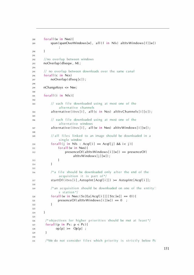
288 f o r a l l (w in Nws) 289 span ( spanOverWindows[w] , a l l ( f in Nfs ) altItvWindows [ f ] [w] )
;290 291
292 / / no overlap between windows293 noOverlap ( dlseqw , M) ;294
295 / / no overlap between downloads over the same canal296 f o r a l l ( c in Ncs )297 noOverlap ( dlseq [c ] ) ;298
299 nChangeKeys <= Nsw;300
301 f o r a l l ( i in Nfs ) 302
303 / / each f i l e downloaded using at most one of thea l t e rna t i ve channels
304 a l t e rna t i ve ( i t v s [ i ] , a l l ( c in Ncs ) a l t I tvChannels [ i ] [ c ] ) ;305
306 / / each f i l e downloaded using at most one of thea l t e rna t i ve windows
307 a l t e rna t i ve ( i t v s [ i ] , a l l (w in Nws) altItvWindows [ i ] [w] ) ;308
309 / / a l l f i l e s l inked to an image should be downloaded in as ing le window
310 f o r a l l ( j in Nfs : Acqf [ i ] == Acqf [ j ] && i < j ) 311 f o r a l l (w in Nws) 312 presenceOf ( altItvWindows [ i ] [w] ) == presenceOf (
altItvWindows [ j ] [w] ) ;313 314 315
316 / * a f i l e should be downloaded only a f t e r the end of theacquis i t ion i t i s par t of * /
317 s ta r tOf ( i t v s [ i ] , AstopInt [Acqf [ i ] ] ) >= AstopInt [Acqf [ i ] ] ;318
319 / * an acquis i t ion should be downloaded on one of the en t i t ys s t a t i on * /
320 f o r a l l (w in Nws: ( Ss [ Ea [Acqf [ i ] ] ] [ Stc [w] ] == 0) ) 321 presenceOf ( altItvWindows [ i ] [w] ) == 0 ;322 323
324 325
326 / * object ives fo r higher p r i o r i t i e s should be met at l e a s t * /327 f o r a l l ( p in Ps : p < Pc ) 328 op[p] >= Op[p] ;329 330
331 / *We do not consider f i l e s which p r i o r i t y i s s t r i c t l y below Pc
151

C. OPL
* /332 f o r a l l ( f in Nfs : Pa [Acqf [ f ] ] > Pc ) 333 presenceOf ( i t v s [ f ] ) == 0 ;334 335
336
152

Quatrième partie
Résumé étendu
153

Introduction 9
L’observation de la Terre depuis l’espace est utile dans de nombreux domainescomme la météorologie, la géodésie, la modélisation du climat, la gestion des catas-trophes naturelles, ou la reconnaissance militaire. Le système spatial que nous consi-dérons est composé de satellites orbitant autour de la Terre. Ces derniers sont équipésd’instruments optiques à haute résolution, qui permettent d’acquérir des images pourdes utilisateurs civils ou militaires, et communiquent avec un réseau de stations sol.Les données acquises sont ensuite compressées, enregistrées, et télé-déchargées (ouvidées) au sol. Les utilisateurs du systèmes soumettent des requêtes d’observation aucentre de mission qui produit des plans d’activités qui sont envoyés aux satellites.Ces plans contiennent plusieurs types d’actions tels que les manœuvres orbitales, lesacquisitions ou les vidages.
Un aspect à ne pas négliger lors de la plani cation d’activités pour des satellitesd’observation est que ceux-ci évoluent dans un environnement dynamique où desévénements imprévus arrivent, comme des changements météorologiques ou des re-quêtes d’observation urgentes. Plusieurs paramètres sont incertains lorsque la plani-cation des activités est réalisée au sol, comme la couverture nuageuse ou la quan-
tité d’énergie disponible à bord. Jusqu’à aujourd’hui, les plans d’activités ne doiventpas être modi és à bord. Ils doivent donc être robustes aux incertitudes pour ne pasmettre le satellite dans un état non désiré. Cela implique d’une part, que toutes lesdécisions sont prises hors-ligne au sol et que le satellite ne fait qu’exécuter strictementle plan sans le modi er d’aucune façon, et d’autre part, que des hypothèses de pirescénario concernant les paramètres incertains sont considérées. Cela rend la plani -cation pessimiste et les plans en résultant sont sous-optimaux. Dans ce contexte, cesincertitudes rendent la plani cation et l’ordonnancement hors-ligne des activités deplus en plus discutables. L’objectif de ce travail est d’améliorer les performances endonnant plus d’autonomie au satellite pour la prise de décision sans compromettrela prévisibilité requise pour certaines activités. L’idée principale est alors de partagerle processus de décision entre le sol et le bord de manière à pro ter des capacitésde calcul au sol et de la faible incertitude restant à bord. D’abord, on applique cetteidée au vidage des acquisitions qui consiste à ordonnancer des télé-déchargements dechiers durant des fenêtres de visibilité satellite/station sol. Puis, on applique cette
idée à la plani cation des observations.
Contexte industriel : le programme OTOSEn 2011 et 2012, deux satellites agile d’observation de la Terre, Pléiades-1A et
Pléiades-1B, ont été mis en orbite par des fusées Soyouz lancées du Centre SpatialGuyanais. Ce programme de coopération entre la France et l’Italie a été géré par leCentre National d’Etudes Spatiales (CNES). Plusieurs pays européens ont contribuéà ce programme comme la Suède (calculateurs de bord) ou l’Espagne (antenne bandeS).
OTOS est un programme technologique dont le but est d’améliorer les perfor-mances de ces systèmes d’observations tout en diminuant leur coût. Les paramètres àaméliorer incluent la résolution d’image (la surface réelle couverte par un pixel, la ré-solution actuelle allant jusqu’à 20cm2 par pixel), la précision altimétrique pour mesu-rer des reliefs, et le nombre de bandes spectrales (le nombre de fréquences auxquelles
155
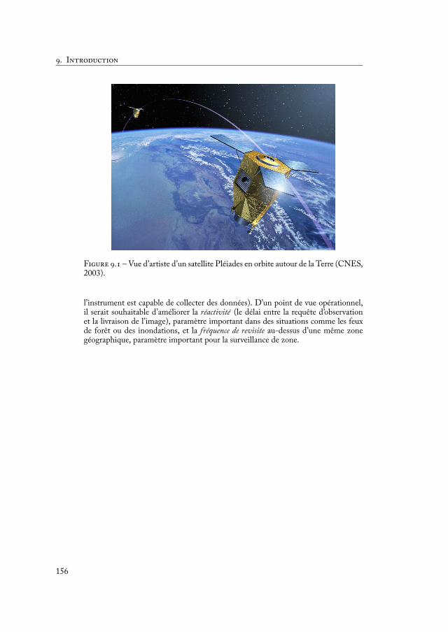
. I
F . – Vue d’artiste d’un satellite Pléiades en orbite autour de la Terre (CNES,2003).
l’instrument est capable de collecter des données). D’un point de vue opérationnel,il serait souhaitable d’améliorer la réactivité (le délai entre la requête d’observationet la livraison de l’image), paramètre important dans des situations comme les feuxde forêt ou des inondations, et la fréquence de revisite au-dessus d’une même zonegéographique, paramètre important pour la surveillance de zone.
156
Contexte applicatif 10
10.1 Architecture du système . . . . . . . . . . . . . . . . . . . . 15510.1.1 Centre de mission . . . . . . . . . . . . . . . . . . 15510.1.2 Stations de contrôle . . . . . . . . . . . . . . . . . 15510.1.3 Stations de réception . . . . . . . . . . . . . . . . 15610.1.4 Utilisateurs, requêtes d’observation et centres de pro-
duction . . . . . . . . . . . . . . . . . . . . . . . 15710.1.5 Satellite géostationnaire . . . . . . . . . . . . . . . 158
10.2 Caractéristiques des satellites d’observation de la Terre . . . . 15810.2.1 Orbite . . . . . . . . . . . . . . . . . . . . . . . . 15810.2.2 Plateforme . . . . . . . . . . . . . . . . . . . . . . 15910.2.3 Chaîne d’acquisition image . . . . . . . . . . . . . 161
10.3 Processus de décision et incertitudes . . . . . . . . . . . . . 165
Dans ce chapitre, on décrit les éléments d’une mission typique d’observation dela Terre, les différents acteurs impliqués, et le processus de décision permettant laplani cation des activités.
Le système spatial que l’on considère est constitué d’un satellite agile d’observationde la Terre (voir Section 10.2.2), de plusieurs stations sol de contrôle, de plusieursstations sol de réception, et de plusieurs centres de traitement des données, chacunassociés avec un utilisateur du système. Dans les paragraphes suivants, on décrit lesdifférents éléments du système (voir Figure 10.1).
10.1 Architecture du systèmeIl y a un segment sol, que l’on décrit ci-dessous, et un satellite d’observation de la
Terre, que l’on décrit en Section 10.2.
10.1.1 Centre de missionLe centre de mission reçoit les requêtes d’observations de la part des utilisateurs
du système et produit des plans d’acquisition et de vidage. Ces plans sont ensuitetransmis à des stations de contrôle. Le processus de plani cation est complexe et denombreux échanges, non détaillés ici, entre les entités peuvent être nécessaire pourvalider les plans d’activités.
10.1.2 Stations de contrôleLes stations de contrôle reçoivent les plans d’activité produits par le centre de
mission et les téléchargent à bord du satellite. Elles reçoivent aussi ce qu’on appelle latélémétrie de servitude. Cette dernière est un ensemble d’informations envoyé depuisle satellite qui permet de véri er que tous les systèmes bord fonctionnent correcte-ment. Les stations de contrôle reçoivent aussi la liste des observations effectuées, laliste des observations supprimées de la mémoire, et la liste des observations vidées.Les stations de contrôle sont réparties sur la surface du globe. Par exemple, le CNES
157

. C
F . – Architecture du système.
a accès au réseau suivant de stations de contrôle : Kerguelen dans les îles Kerguelen ;Kiruna en Suède ; Aussaguel en France ; Kourou en Guyane Française ; Hartebees-thoek en Afrique du Sud ; Perth en Australie. Toutes ces stations sont connectéesavec le centre de mission par un lien haut-débit.
10.1.3 Stations de réceptionLes stations de réception sont exclusivement utilisées pour recevoir de la télémétrie
mission qui correspond aux données collectées par les instruments de la charge utiledu satellite (des images dans notre cas). Ces données peuvent être transférées quandle satellite est en visibilité, c’est à dire quand son antenne de télémétrie est capable decommuniquer avec l’antenne de la station. Chaque utilisateur a une ou plusieurs sta-tions autorisées pour le vidage des données. Les acquisitions reçues dans une stationde réception sont ensuite envoyées dans le centre de production associé à l’utilisateurdemandeur.
158

10.1. Architecture du système
La liste des acquisitions vidées et la liste des acquisitions stockées en mémoireà bord du satellite sont envoyées au centre de mission. Notons qu’il est importantde maintenir la cohérence entre l’état de la connaissance entre les stations sol et lesatellite de façon à ce que les algorithmes sol puissent s’appuyer sur les données lesplus récentes pour produire des plans. Pourtant, ce n’est pas toujours possible, à causedes délais de transfert au sol par exemple. Il est nécessaire de penser à la réparationdu plan lors de l’exécution quand le plan produit au sol n’est plus cohérent avec l’étatréel du satellite (comme par exemple un plan de vidage qui contient le vidage d’uneacquisition qui a déjà été effacée à bord).
10.1.4 Utilisateurs, requêtes d’observation et centres de productionLes requêtes d’observation sont émises par les utilisateurs du système. Chaque
observation est dé nie par :– une zone géographique à observer qui est un polygone découpé en bandes (voir
Figure10.2) ; chaque bande est référencée par ses coordonnées géographiques,une durée d’observation, et un volume de données ; et parfois des prévisionsmétéo pour la zone ; l’observation doit être réalisée dans une des fenêtres devisibilité de la bande ;
– un niveau de priorité ; les priorités sont dites étanches car il est toujours pré-férable de satisfaire une requête de haute priorité plutôt que n’importe quelensemble de requêtes de plus basse priorité ;
– un poids, permettant de trier les acquisitions qui ont le même niveau de prio-rité ;
– des angles d’observation maximum : plus l’angle d’observation est grand, moinsla qualité est bonne ; la meilleure qualité est donnée par un pointage nadir, c’està dire quand le satellite pointe vers le centre de la Terre.
polygon
strip
possible
acquired
directions
swath
F . – Une zone géographique découpée en bandes.
Une fois que les observations ont été réalisées, les données brutes associées sontenvoyées vers les centres de production qui les transforment en images livrables.Chaque utilisateur du système a son centre de production préféré.
159
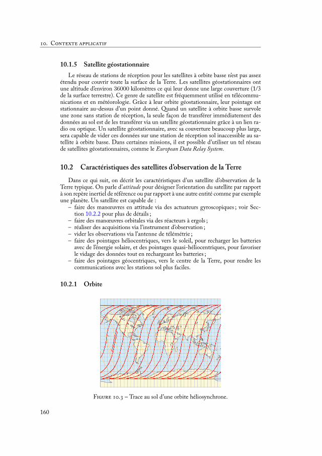
. C
10.1.5 Satellite géostationnaireLe réseau de stations de réception pour les satellites à orbite basse n’est pas assez
étendu pour couvrir toute la surface de la Terre. Les satellites géostationnaires ontune altitude d’environ 36000 kilomètres ce qui leur donne une large couverture (1/3de la surface terrestre). Ce genre de satellite est fréquemment utilisé en télécommu-nications et en météorologie. Grâce à leur orbite géostationnaire, leur pointage eststationnaire au-dessus d’un point donné. Quand un satellite à orbite basse survoleune zone sans station de réception, la seule façon de transférer immédiatement desdonnées au sol est de les transférer via un satellite géostationnaire grâce à un lien ra-dio ou optique. Un satellite géostationnaire, avec sa couverture beaucoup plus large,sera capable de vider ces données sur une station de réception sol inaccessible au sa-tellite à orbite basse. Dans certaines missions, il est possible d’utiliser un tel réseaude satellites géostationnaires, comme le European Data Relay System.
10.2 Caractéristiques des satellites d’observation de la TerreDans ce qui suit, on décrit les caractéristiques d’un satellite d’observation de la
Terre typique. On parle d’attitude pour désigner l’orientation du satellite par rapportà son repère inertiel de référence ou par rapport à une autre entité comme par exempleune planète. Un satellite est capable de :
– faire des manœuvres en attitude via des actuateurs gyroscopiques ; voir Sec-tion 10.2.2 pour plus de détails ;
– faire des manœuvres orbitales via des réacteurs à ergols ;– réaliser des acquisitions via l’instrument d’observation ;– vider les observations via l’antenne de télémétrie ;– faire des pointages héliocentriques, vers le soleil, pour recharger les batteries
avec de l’énergie solaire, et des pointages quasi-héliocentriques, pour favoriserle vidage des données tout en rechargeant les batteries ;
– faire des pointages géocentriques, vers le centre de la Terre, pour rendre lescommunications avec les stations sol plus faciles.
10.2.1 Orbite
F . – Trace au sol d’une orbite héliosynchrone.
160
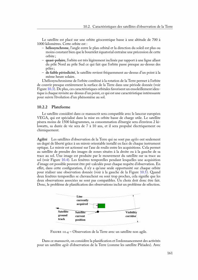
10.2. Caractéristiques des satellites d’observation de la Terre
Le satellite est placé sur une orbite géocentrique basse à une altitude de 700 à1000 kilomètres. Cette orbite est :
– héliosynchrone, l’angle entre le plan orbital et la direction du soleil est plus oumoins constant bien que le bourrelet équatorial entraîne une précession de cetteorbite ;
– quasi-polaire, l’orbite est très légèrement inclinée par rapport à une ligne allantdu pôle Nord au pôle Sud ce qui fait que l’orbite passe presque au-dessus despôles ;
– de faible périodicité, le satellite revient fréquemment au-dessus d’un point à lamême heure solaire.
L’héliosynchronisme de l’orbite combiné à la rotation de la Terre permet à l’orbitede couvrir presque entièrement la surface de la Terre dans une période donnée (voirFigure 10.3). De plus, ces caractéristiques orbitales favorisent un ensoleillement iden-tique à chaque revisite au-dessus d’un point, ce qui est une caractéristique intéressantepour suivre l’évolution d’un phénomène au sol.
10.2.2 PlateformeLe satellite considéré dans ce manuscrit sera compatible avec le lanceur européen
VEGA, qui est spécialisé dans la mise en orbite basse de charge utile. Le satellitepèsera moins de 1500 kilogrammes, sa consommation d’énergie sera d’environ 2 ki-lowatts, sa durée de vie sera de 7 à 10 ans, et il sera propulsé électriquement ouchimiquement.
Agilité Les satellites d’observation de la Terre qui ne sont pas agiles ont seulementun degré de liberté grâce à un miroir orientable installé en face de chaque instrumentoptique. Le miroir est actionné sur l’axe de roulis entre les acquisitions. Cela permetau satellite de prendre des images de zones situées à la droite ou à la gauche de satrace au sol. Une image est produite par le mouvement du satellite sur sa trace ausol (voir Figure 10.4). Les fenêtres temporelles pendant lesquelles une acquisitiond’image est possible peuvent être pré-calculée pour chaque requête d’observation. Eneffet, dans cette con guration, il n’y a qu’une seule opportunité sur chaque orbitepour réaliser une observation donnée (voir à la gauche de la Figure 10.5). Quanddeux fenêtres temporelles se chevauchent ou sont trop proches, cela signi e que lesdeux observations associées ne sont pas compatibles. Un choix doit donc être fait.Donc, le problème de plani cation des observations inclut un problème de sélection.
F . – Observation de la Terre avec un satellite non agile.
Dans ce manuscrit, on considère la plani cation et l’ordonnancement des activitéspour un satellite agile d’observation de la Terre (comme les satellite Pléiades). Avec
161

. C
ce type de satellite, les instruments et les panneaux solaires sont xés (body-mounted)sur la plateforme (pour éviter les perturbations d’attitude à basse fréquence), et c’estla plateforme qui est mobile sur les trois axes (roulis, tangage et lacet) grâce à desactionneurs gyroscopiques [Chrétien et al., 2004]. Ces deux axes d’agilité supplé-mentaires permettent de décupler les opportunités pour chaque image. En effet, lesatellite peut maintenant pointer en avant ou en arrière de sa position nadir (voir Fi-gure 10.6). Le début d’une acquisition devient libre dans une fenêtre temporelle quipeut être pré-calculée (voir Figure 10.5). Ces fenêtres temporelles sont plus grandesque dans le cas non agile, et certaines acquisitions qui n’étaient pas compatibles de-viennent compatibles grâce à cette agilité (voir à la droite de la Figure 10.5). Leproblème de plani cation résultant inclut un problème de sélection et un problèmed’ordonnancement, le rendant plus difficile.
corridorVisibility
Observationwindow
Satellitegroundtrack
observation
observation
corridorVisibility
Observationwindow
Visibilitywindow
Candidate
SelectedSatellitegroundtrack
F . – Comparaison des capacités d’observations entre un satellite non agile(gauche) et un satellite agile (droite).
De plus, dans le cas des satellites agiles, la durée minimum de transition entredeux observations successives depend de la date de début de la transition (voir Fi-gure 10.6). Calculer ces durées minimum est un problème d’optimisation continusous contraintes [Beaumet et al., 2007], qui peut être résolu en utilisant des solveurstels que RealPaver [Granvilliers and Benhamou, 2006] ou IBEX [Chabert and Jaulin,2009], ou des techniques d’approximation.
La capacité du satellite à faire des mouvements en attitude combinée à sa trajec-toire orbitale permet de réaliser des acquisitions en scannant la zone à acquérir. Les
162
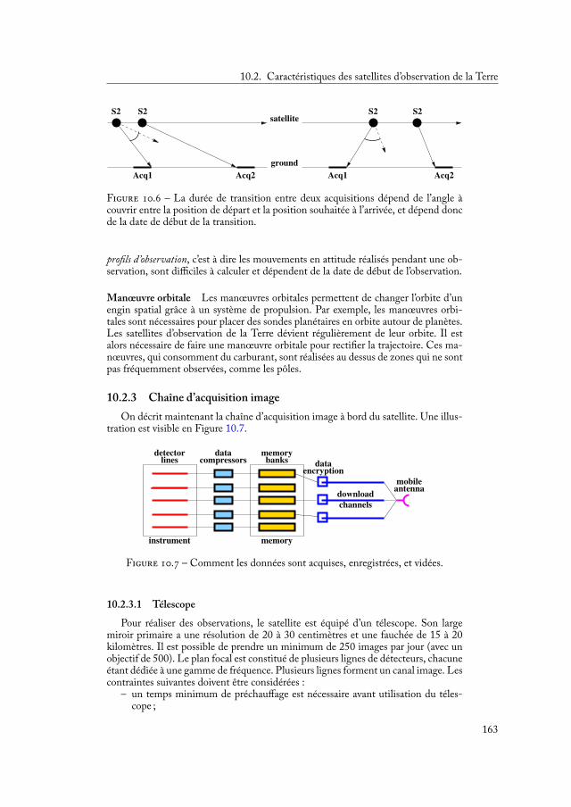
10.2. Caractéristiques des satellites d’observation de la Terre
S2 S2 S2 S2
ground
satellite
Acq1 Acq2 Acq1 Acq2
F . – La durée de transition entre deux acquisitions dépend de l’angle àcouvrir entre la position de départ et la position souhaitée à l’arrivée, et dépend doncde la date de début de la transition.
pro ls d’observation, c’est à dire les mouvements en attitude réalisés pendant une ob-servation, sont difficiles à calculer et dépendent de la date de début de l’observation.
Manœuvre orbitale Les manœuvres orbitales permettent de changer l’orbite d’unengin spatial grâce à un système de propulsion. Par exemple, les manœuvres orbi-tales sont nécessaires pour placer des sondes planétaires en orbite autour de planètes.Les satellites d’observation de la Terre dévient régulièrement de leur orbite. Il estalors nécessaire de faire une manœuvre orbitale pour recti er la trajectoire. Ces ma-nœuvres, qui consomment du carburant, sont réalisées au dessus de zones qui ne sontpas fréquemment observées, comme les pôles.
10.2.3 Chaîne d’acquisition imageOn décrit maintenant la chaîne d’acquisition image à bord du satellite. Une illus-
tration est visible en Figure 10.7.
encryption
download
channels
instrument memory
memorybanks
datacompressors
detectorlines data
antennamobile
F . – Comment les données sont acquises, enregistrées, et vidées.
10.2.3.1 TélescopePour réaliser des observations, le satellite est équipé d’un télescope. Son large
miroir primaire a une résolution de 20 à 30 centimètres et une fauchée de 15 à 20kilomètres. Il est possible de prendre un minimum de 250 images par jour (avec unobjectif de 500). Le plan focal est constitué de plusieurs lignes de détecteurs, chacuneétant dédiée à une gamme de fréquence. Plusieurs lignes forment un canal image. Lescontraintes suivantes doivent être considérées :
– un temps minimum de préchauffage est nécessaire avant utilisation du téles-cope ;
163
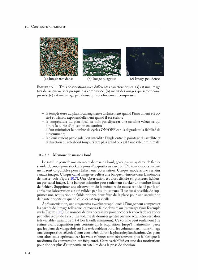
. C
(a) Image très dense (b) Image nuageuse (c) Image peu dense
F . – Trois observations avec différentes caractéristiques. (a) est une imagetrès dense qui ne sera presque pas compressée. (b) inclut des nuages qui seront com-pressés. (c) est une image peu dense qui sera fortement compressée.
– la température du plan focal augmente linéairement quand l’instrument est ac-tivé et décroit exponentiellement quand il est éteint ;
– la température du plan focal ne doit pas dépasser une certaine valeur ce quilimite la durée d’utilisation en continu ;
– il faut minimiser le nombre de cycles ON/OFF car ils dégradent la abilité del’instrument ;
– l’éblouissement par le soleil est interdit : l’angle entre le pointage du satellite etla direction du soleil doit toujours être plus grand ou égal à une valeur minimale.
10.2.3.2 Mémoire de masse à bord
Le satellite possède une mémoire de masse à bord, gérée par un système de chierstandard, conçu pour stocker 2 jours d’acquisitions environ. Plusieurs modes instru-ment sont disponibles pour réaliser une observation. Chaque mode active certainscanaux images. Chaque canal image est relié à une banque mémoire dans la mémoirede masse (voir Figure 10.7). Une observation est alors divisée en plusieurs chiers,un par canal image. Une banque mémoire peut seulement stocker un nombre limitéde chiers. Supprimer une observation de la mémoire de masse est décidé par le solaprès que l’observation ait été validée par les utilisateurs. Il est aussi possible de sup-primer une acquisition de faible priorité pour faire de la place pour une acquisitionde haute priorité ou quand celle-ci est trop vieille.
Après acquisition, une compression sélective est appliquée à l’image pour compresserles parties de l’image telles que les zones à faible densité ou les nuages (voir l’exemplesur la Figure 10.8). Le nombre de bits nécessaires pour encoder les pixels de ces zonespeut être réduit de 12 à 3. Le volume de données généré par une acquisition est alorstrès variable (variant de 1 à 4 fois la taille minimum). Ce volume peut seulement êtreestimé avant acquisition puis constaté après acquisition. Jusqu’à maintenant, parceque les plans de vidage doivent être exécutables à bord, les volumes maximums (imagesans compression sélective) sont considérés durant la phase de plani cation. Ces planssont alors sous-optimaux car les vrais volumes sont très souvent plus faibles que lemaximum (la compression est fréquente). Cette variabilité est une des motivationspour donner plus d’autonomie au satellite dans la prise de décision.
164
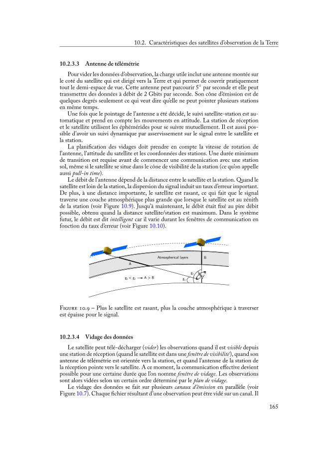
10.2. Caractéristiques des satellites d’observation de la Terre
10.2.3.3 Antenne de télémétriePour vider les données d’observation, la charge utile inclut une antenne montée sur
le coté du satellite qui est dirigé vers la Terre et qui permet de couvrir pratiquementtout le demi-espace de vue. Cette antenne peut parcourir 5 par seconde et elle peuttransmettre des données à débit de 2 Gbits par seconde. Son cône d’émission est dequelques degrés seulement ce qui veut dire qu’elle ne peut pointer plusieurs stationsen même temps.
Une fois que le pointage de l’antenne a été décidé, le suivi satellite-station est au-tomatique et prend en compte les mouvements en attitude. La station de réceptionet le satellite utilisent les éphémérides pour se suivre mutuellement. Il est aussi pos-sible d’avoir un suivi dynamique par asservissement sur le signal entre le satellite etla station.
La plani cation des vidages doit prendre en compte la vitesse de rotation del’antenne, l’attitude du satellite et les coordonnées des stations. Une durée minimumde transition est requise avant de commencer une communication avec une stationsol, même si le satellite se situe dans le cône de visibilité de la station (ce qu’on appelleaussi pull-in time).
Le débit de l’antenne dépend de la distance entre le satellite et la station. Quand lesatellite est loin de la station, la dispersion du signal induit un taux d’erreur important.De plus, à une distance importante, le satellite est rasant, ce qui fait que le signaltraverse une couche atmosphérique plus grande que lorsque le satellite est au zénithde la station (voir Figure 10.9). Jusqu’à maintenant, le débit était xé au pire débitpossible, obtenu quand la distance satellite/station est maximum. Dans le systèmefutur, le débit est dit intelligent car il varie durant les fenêtres de communication enfonction du taux d’erreur (voir Figure 10.10).
F . – Plus le satellite est rasant, plus la couche atmosphérique à traverserest épaisse pour le signal.
10.2.3.4 Vidage des donnéesLe satellite peut télé-décharger (vider) les observations quand il est visible depuis
une station de réception (quand le satellite est dans une fenêtre de visibilité ), quand sonantenne de télémétrie est orientée vers la station, et quand l’antenne de la station dela réception pointe vers le satellite. A ce moment, la communication effective devientpossible pour une certaine durée que l’on nomme fenêtre de vidage. Les observationssont alors vidées selon un certain ordre déterminé par le plan de vidage.
Le vidage des données se fait sur plusieurs canaux d’émission en parallèle (voirFigure 10.7). Chaque chier résultant d’une observation peut être vidé sur un canal. Il
165
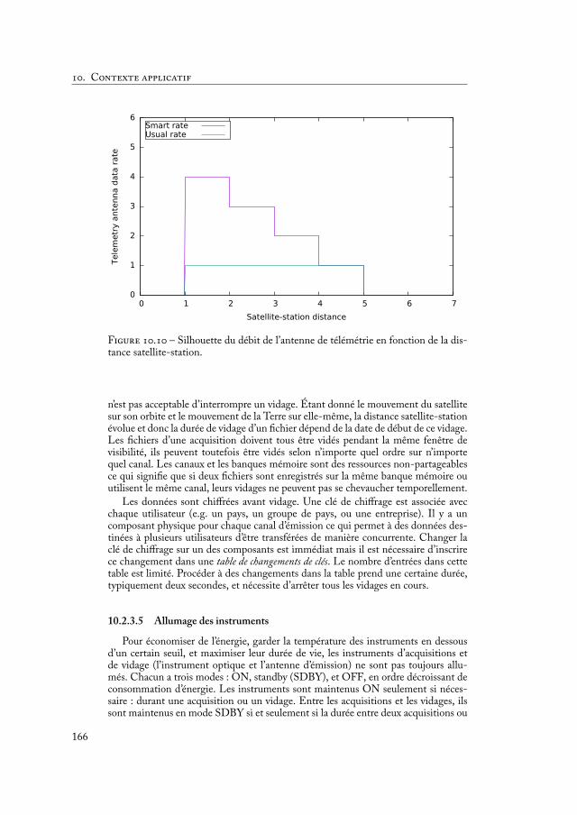
. C
0
1
2
3
4
5
6
0 1 2 3 4 5 6 7
Tele
met
ry a
nten
na d
ata
rate
Satellite-station distance
Smart rateUsual rate
F . – Silhouette du débit de l’antenne de télémétrie en fonction de la dis-tance satellite-station.
n’est pas acceptable d’interrompre un vidage. Étant donné le mouvement du satellitesur son orbite et le mouvement de la Terre sur elle-même, la distance satellite-stationévolue et donc la durée de vidage d’un chier dépend de la date de début de ce vidage.Les chiers d’une acquisition doivent tous être vidés pendant la même fenêtre devisibilité, ils peuvent toutefois être vidés selon n’importe quel ordre sur n’importequel canal. Les canaux et les banques mémoire sont des ressources non-partageablesce qui signi e que si deux chiers sont enregistrés sur la même banque mémoire ouutilisent le même canal, leurs vidages ne peuvent pas se chevaucher temporellement.
Les données sont chiffrées avant vidage. Une clé de chiffrage est associée avecchaque utilisateur (e.g. un pays, un groupe de pays, ou une entreprise). Il y a uncomposant physique pour chaque canal d’émission ce qui permet à des données des-tinées à plusieurs utilisateurs d’être transférées de manière concurrente. Changer laclé de chiffrage sur un des composants est immédiat mais il est nécessaire d’inscrirece changement dans une table de changements de clés. Le nombre d’entrées dans cettetable est limité. Procéder à des changements dans la table prend une certaine durée,typiquement deux secondes, et nécessite d’arrêter tous les vidages en cours.
10.2.3.5 Allumage des instruments
Pour économiser de l’énergie, garder la température des instruments en dessousd’un certain seuil, et maximiser leur durée de vie, les instruments d’acquisitions etde vidage (l’instrument optique et l’antenne d’émission) ne sont pas toujours allu-més. Chacun a trois modes : ON, standby (SDBY), et OFF, en ordre décroissant deconsommation d’énergie. Les instruments sont maintenus ON seulement si néces-saire : durant une acquisition ou un vidage. Entre les acquisitions et les vidages, ilssont maintenus en mode SDBY si et seulement si la durée entre deux acquisitions ou
166
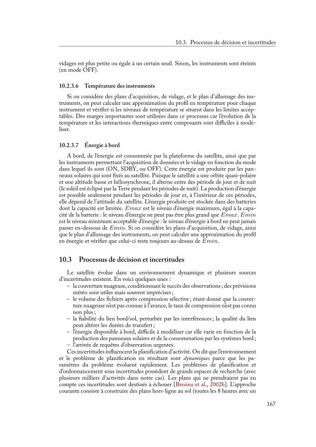
10.3. Processus de décision et incertitudes
vidages est plus petite ou égale à un certain seuil. Sinon, les instruments sont éteints(en mode OFF).
10.2.3.6 Température des instrumentsSi on considère des plans d’acquisition, de vidage, et le plan d’allumage des ins-
truments, on peut calculer une approximation du pro l en température pour chaqueinstrument et véri er si les niveaux de température se situent dans les limites accep-tables. Des marges importantes sont utilisées dans ce processus car l’évolution de latempérature et les interactions thermiques entre composants sont difficiles à modé-liser.
10.2.3.7 Énergie à bordA bord, de l’énergie est consommée par la plateforme du satellite, ainsi que par
les instruments permettant l’acquisition de données et le vidage en fonction du modedans lequel ils sont (ON, SDBY, ou OFF). Cette énergie est produite par les pan-neaux solaires qui sont xés au satellite. Puisque le satellite a une orbite quasi-polaireet une altitude basse et héliosynchrone, il alterne entre des période de jour et de nuit(le soleil est éclipsé par la Terre pendant les périodes de nuit). La production d’énergieest possible seulement pendant les périodes de jour et, à l’intérieur de ces périodes,elle dépend de l’attitude du satellite. L’énergie produite est stockée dans des batteriesdont la capacité est limitée. Emax est le niveau d’énergie maximum, égal à la capa-cité de la batterie : le niveau d’énergie ne peut pas être plus grand que Emax. Eminest le niveau minimum acceptable d’énergie : le niveau d’énergie à bord ne peut jamaispasser en-dessous de Emin. Si on considère les plans d’acquisition, de vidage, ainsique le plan d’allumage des instruments, on peut calculer une approximation du pro len énergie et véri er que celui-ci reste toujours au-dessus de Emin.
10.3 Processus de décision et incertitudesLe satellite évolue dans un environnement dynamique et plusieurs sources
d’incertitudes existent. En voici quelques unes :– la couverture nuageuse, conditionnant le succès des observations ; des prévisions
météo sont utiles mais souvent imprécises ;– le volume des chiers après compression sélective ; étant donné que la couver-
ture nuageuse n’est pas connue à l’avance, le taux de compression n’est pas connunon plus ;
– la abilité du lien bord/sol, perturbée par les interférences ; la qualité du lienpeut altérer les durées de transfert ;
– l’énergie disponible à bord, difficile à modéliser car elle varie en fonction de laproduction des panneaux solaires et de la consommation par les systèmes bord ;
– l’arrivée de requêtes d’observation urgentes.Ces incertitudes in uencent la plani cation d’activité. On dit que l’environnement
et le problème de plani cation en résultant sont dynamiques parce que les pa-ramètres du problème évoluent rapidement. Les problèmes de plani cation etd’ordonnancement sous incertitudes possèdent de grands espaces de recherche (avecplusieurs milliers d’activités dans notre cas). Les plans qui ne prendraient pas encompte ces incertitudes sont destinés à échouer [Bresina et al., 2002b]. L’approchecourante consiste à construire des plans hors-ligne au sol (toutes les 8 heures avec un
167

. C
F . – Vue générale du processus de construction des plans d’acquisition,de vidage, et d’allumage des instruments.
horizon glissant de 24 heures), dans lesquels les activités ont des dates de début et den xées. Toutes les contraintes relatives à l’attitude du satellite, à l’acquisition et au
vidage, à l’énergie, à la mémoire, et à la température, sont véri ées au sol. Pour êtrecertain que les plans soient exécutables sans changements, des marges de sureté sontutilisées tout au long du processus. Par exemple la production d’énergie espérée estremplacée par la pire production possible. Cela résulte en un problème encore pluscontraint. Les plans sont ensuite envoyés au satellite durant une fenêtre de visibilitéde station de contrôle et exécutés strictement par le satellite.
Le but de cette thèse est d’aller au-delà de ce schéma et d’améliorer les perfor-mances par une meilleure gestion des incertitudes. Dans le prochain chapitre, nousverrons les différentes façon d’organiser la décision pour parvenir à cela dans le cas dela plani cation des vidages.
168

Ordonnancement exible des vidages 11
11.1 Description du problème de vidage . . . . . . . . . . . . . . 16811.2 Plusieurs processus de décision . . . . . . . . . . . . . . . . 172
11.2.1 Aperçu de l’approche sol . . . . . . . . . . . . . . . 17211.2.2 Aperçu de l’approche bord . . . . . . . . . . . . . . 17311.2.3 Aperçu de l’approche mixte sol-bord . . . . . . . . . 175
11.3 Expérimentations . . . . . . . . . . . . . . . . . . . . . . . 17711.3.1 Approches à comparer . . . . . . . . . . . . . . . . 17711.3.2 Scénarios . . . . . . . . . . . . . . . . . . . . . . 17811.3.3 Critères d’évaluation . . . . . . . . . . . . . . . . . 17911.3.4 Analyse des résultats . . . . . . . . . . . . . . . . . 179
Notre première contribution 1 concerne le problème de vidage des acquisitionsqui consiste à ordonnancer des vidages de chiers durant des fenêtres de communi-cation entre le satellite et les stations de réception sol. Des algorithmes sophistiquéscompressent les zones de faible intérêt sur les images acquises à bord, comme parexemple les nuages ou les terrains uniformes. Ainsi, la quantité de données résultantd’une acquisition, devant être enregistrée à bord, et ensuite vidée au sol est imprévi-sible puisque qu’elle dépendra des données acquises et de l’environnement à l’instantde la prise de vue.
Comme il n’est pas possible de communiquer continuellement avec les satellites,les volumes de données générés sont d’abord connus à bord avant de pouvoir êtrecommuniqués au sol. Cela mène à penser que les décisions concernant les vidagesdevraient être prises à bord juste avant les fenêtres de communication avec les sta-tions sol. A ce moment les volumes réel des données sont connus et la plani cationà bord peut donc produire des plans d’une grande qualité. Cependant la plani ca-tion à bord prend du temps et des ressources informatiques importantes. De plus, lesplans produits ne sont pas connus au sol avant leur exécution et le comportement dusatellite est donc imprévisible du point de vue du contrôle opérationnel au sol. Celaest problématique, particulièrement pour les acquisitions de haute priorité car les uti-lisateurs ayant demandé ces acquisitions peuvent parfois exiger de savoir quand lesdonnées seront disponibles. Dans ces conditions, il est toujours possible de construiredes plans de vidage au sol avec des hypothèses pire-cas sur les volumes de données,c’est à dire en supposant que tous les volumes sont maximum (cela correspondant àsupposer que la compression à bord sera minimale). Ces plans seront toujours exécu-tables à bord mais largement sous-optimaux étant donné que les fenêtres de vidagesseront sous-utilisées en réalité puisque les volumes effectifs sont bien souvent plusfaibles que le maximum.
Dans ce travail, nous introduisons un mécanisme qui résulte en plus d’autonomieà bord du satellite mais qui conserve une certaine prévisibilité pour les opérateurs au
1. Cette partie du travail a été présentée aux conférences nationales et internationales suivantes :ICAPS’14 [Pralet et al., 2014c], ICAPS’15 [Maillard et al., 2015a], i-SAIRAS’14 [Maillard et al., 2014],JFPC’14 [Pralet et al., 2014a], ROADEF’14, et ROADEF’15. Un article concernant l’approche mixte sol-bord pour le vidage des acquisitions a été accepté dans AIAA J A I S -
. Un article développant des aspects théoriques du sous-problème d’ordonnancement des vidages dechiers est actuellement revu pour publication dans D A M .
169
. O
sol. Le problème de vidage est un problème complexe d’ordonnancement avec descontraintes temporelles et non temporelles, proche de problèmes de type RCPSP/-max ou exible job-shop. Cependant, aucune technique existante ne peut être direc-tement appliquée à notre problème car celui-ci présente des caractéristiques particu-lières telles que des contraintes temporelles de type time-dependent ou un objectif dejuste répartition de la ressource dans le critère d’optimisation. Pour résoudre ce pro-blème, l’idée est de construire des plans de vidages au sol et d’utiliser l’information laplus récente concernant les volumes pour adapter ce plan à bord. Plus précisément,un ordonnancement est produit au sol avec des hypothèses de volumes maximumspour les acquisitions de haute priorité et des hypothèses de volumes moyens pour lesacquisitions de faible priorité. La plani cation au sol sur un large horizon temporelavec des capacités de calcul suffisantes permet de produire des plans de bonne qualitéet de prendre en compte un critère d’optimisation complexe incluant la juste répar-tition de l’utilisation du système parmi les utilisateurs ou la minimisation de l’agede l’information, ce qui ne serait pas possible à bord. Pour faire cela, on utilise unalgorithme de type Squeaky Wheel Optimization au-dessus d’un algorithme gloutonnon-chronologique. Les nombreuses contraintes du problème sont véri ées avec lalibrairie InCELL. De par l’utilisation des volumes moyens pour certaines acquisi-tions, le plan n’est pas directement exécutable à bord. Certains volumes peuvent êtreplus grands que prévus et il faut donc réparer le plan. Une adaptation du plan sol estdonc entreprise avant chaque groupe de fenêtres de visibilité. Un algorithme glou-ton rapide construit un plan exécutable depuis le plan sol en supprimant du plan lesvidages de faible priorité s’ils mettent en danger la réalisation future des vidages dehaute priorité. Des bornes sur la disponibilité des ressources, calculées au sol, per-mettent de véri er rapidement si le volume réel des acquisitions de faible priorité vamettre en danger les vidages futurs. Avec un mécanisme de recherche en avant, onassure que toutes les vidages de haute priorité seront effectués. Quand les volumesréels sont plus faibles que prévus, la procédure d’adaptation essaie d’insérer des vi-dages qui n’étaient pas prévus par le plan sol ou d’avancer des vidages plus tôt dansle plan. L’adaptation à bord permet de pro ter de la connaissance des vrais volumeset de mettre à jour le plan dans un temps acceptable (en comparaison avec la plani -cation totalement à bord). La combinaison de ces deux phases de plani cation dansun mécanisme exible rend cette approche très compétitive, parfois même meilleureque la plani cation purement à bord en terme de critère d’optimisation, et beaucoupplus prévisible que celle-ci.
11.1 Description du problème de vidage
Comme vu précédemment, après que le satellite ait acquis des données, il doitles vider durant une fenêtre de visibilité de station de réception. Dans ce chapitre,on décrit de manière informelle le problème d’ordonnancement des vidages menantà un plan de vidage et les différentes méthodes que nous avons mis en œuvre pourle traiter. Remarquons que les contraintes de ce problème proviennent d’un systèmeréel et qu’elles rendent le problème plus difficile à traiter qu’un problème théoriqued’optimisation.
Dans le reste de ce résumé, les mots observation et acquisition d’un coté, et fenêtrede vidage et fenêtre de visibilité d’un autre coté, se référent au même concept.
Pour bâtir un plan de vidage, des décisions doivent être prises à trois niveauxdifférents :
170
11.1. Description du problème de vidage
1. la sélection, l’affectation et l’ordonnancement des vidages d’observations : celaconsiste à décider quelles observations vont être vidées et à bâtir une séquencede vidages d’observation, chaque vidage étant constitué d’une observation o etd’une fenêtre de vidage w, allouée à o ; ce problème est proche du problème detype multi-sac-à-dos [Kellerer et al., 2004] ou les objets sont les observationset les sacs sont les fenêtres, mais , dans notre cas, les premiers sacs sont pré-férés puisque la fraicheur de l’information doit être maximisée, et des con itspeuvent exister entre sacs (chevauchements entre fenêtres) ;
2. affectation et ordonnancement des chiers : chaque observation génère plu-sieurs chiers ; une fois qu’une observation a été assignée à une fenêtre de vi-dage, ce sous-problème consiste à assigner chaque chier de cette observationà un canal d’émission, et à bâtir pour chaque canal d’émission et chaque banquemémoire, une séquence de vidages de chiers ; dans chaque fenêtre de vi-dage, ce problème est proche du Flexible Open-shop Scheduling problem [Pinedo,2012] avec deux types de ressources non-partageables : canaux et banques mé-moires ; chaque vidage de chier a besoin d’une ressource de chaque type, maisle choix du canal est libre alors que la banque est pré-allouée ; l’ordre de vidagesur les canaux et les tranches est aussi libre ;
3. gestion des dates : cela consiste soit à calculer les dates au plus tôt et au plus tardpour tous les évènements, soit à xer les dates précises ; les événements concer-nés sont les débuts et ns de vidages de chiers, de mouvements d’antenne, etde mises à jour de la table des changements de clés ; le problème temporel ré-sultant a la forme d’un Simple Temporal Network ; la seule exception concerneles durées de vidages de chiers et de transitions entre fenêtres de vidage quisont dépendantes de leurs dates de début (elle sont dites time-dependent) ; lerésultat est un Time-dependent STN, pour lequel les techniques développéessur les STN peuvent être étendues.
Ces décisions doivent satisfaire toutes les contraintes qui sont détaillées ci-après.Beaucoup de celles-ci proviennent des limitations du système physique : par exemple,les durées de vidage. D’autres proviennent de contraintes utilisateur : par exemple, lefait que tous les chiers générés par une observation doivent être vidés sur une sta-tion s et durant une de ses fenêtres de vidage associée. Un autre exemple est la notiond’engagement qui peut être associé à certaines observations, empêchant certaines déci-sions prises au sol d’être modi ées à bord. Plus de détails seront données dans la Sec-tion 11.2.3. Beaucoup de contraintes sont temporelles : par exemple, l’absence de che-vauchement entre vidages de chiers sur les canaux et les tranches. Certaines ne sontpas temporelles : par exemple, le fait qu’une observation demandée par l’utilisateur udoive être vidée sur une station autorisée par u.
Les décisions doivent aussi optimiser un critère global qui prend en compte lesobservations vidées, leurs priorités, l’age de l’information (la distance temporelle entreune observation et la livraison des données à l’utilisateur les ayant demandées), et lajuste répartition du système satellite entre les utilisateurs.
Pour illustrer le problème de plani cation des vidages, voici un exemple. Cetexemple implique deux fenêtres de vidage 1 et 2 se chevauchant respectivement as-sociées avec deux stations de réception 1 et 2, huit observations à vider de A à F ,deux niveaux de priorité 1 et 2, trois utilisateurs numérotés de 1 à 3, cinq banquesmémoire numérotées de 1 à 5, et trois canaux d’émission numérotés de 1 à 3. Le ta-bleau 11.1 montre les priorités et les utilisateurs associés à chaque observation, ainsique les chiers générés par chaque observation et les banques mémoire sur lesquellesceux-ci sont enregistrés. Par exemple, l’observation A est de priorité 2 (faible prio-
171
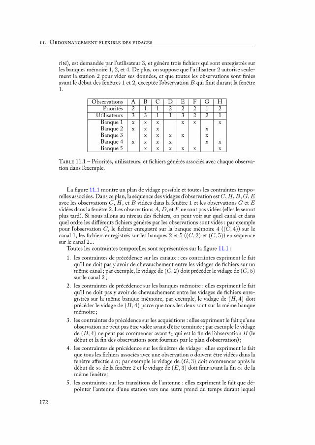
. O
rité), est demandée par l’utilisateur 3, et génère trois chiers qui sont enregistrés surles banques mémoire 1, 2, et 4. De plus, on suppose que l’utilisateur 2 autorise seule-ment la station 2 pour vider ses données, et que toutes les observations sont niesavant le début des fenêtres 1 et 2, exceptée l’observation B qui nit durant la fenêtre1.
Observations A B C D E F G HPriorités 2 1 1 2 2 2 1 2
Utilisateurs 3 3 1 1 3 2 2 1Banque 1 x x x x x xBanque 2 x x x xBanque 3 x x x x xBanque 4 x x x x x xBanque 5 x x x x x x
T 11.1 – Priorités, utilisateurs, et chiers générés associés avec chaque observa-tion dans l’exemple.
La gure 11.1 montre un plan de vidage possible et toutes les contraintes tempo-relles associées. Dans ce plan, la séquence des vidages d’observation est C, H, B, G, Eavec les observations C, H , et B vidées dans la fenêtre 1 et les observations G et Evidées dans la fenêtre 2. Les observations A, D, et F ne sont pas vidées (elles le serontplus tard). Si nous allons au niveau des chiers, on peut voir sur quel canal et dansquel ordre les différents chiers générés par les observations sont vidés : par exemplepour l’observation C, le chier enregistré sur la banque mémoire 4 ((C, 4)) sur lecanal 1, les chiers enregistrés sur les banques 2 et 5 ((C, 2) et (C, 5)) en séquencesur le canal 2...
Toutes les contraintes temporelles sont représentées sur la gure 11.1 :1. les contraintes de précédence sur les canaux : ces contraintes expriment le fait
qu’il ne doit pas y avoir de chevauchement entre les vidages de chiers sur unmême canal ; par exemple, le vidage de (C, 2) doit précéder le vidage de (C, 5)sur le canal 2 ;
2. les contraintes de précédence sur les banques mémoire : elles expriment le faitqu’il ne doit pas y avoir de chevauchement entre les vidages de chiers enre-gistrés sur la même banque mémoire, par exemple, le vidage de (H, 4) doitprécéder le vidage de (B, 4) parce que tous les deux sont sur la même banquemémoire ;
3. les contraintes de précédence sur les acquisitions : elles expriment le fait qu’uneobservation ne peut pas être vidée avant d’être terminée ; par exemple le vidagede (B, 4) ne peut pas commencer avant t1 qui est la n de l’observation B (ledébut et la n des observations sont fournies par le plan d’observation) ;
4. les contraintes de précédence sur les fenêtres de vidage : elles expriment le faitque tous les chiers associés avec une observation o doivent être vidées dans lafenêtre affectée à o ; par exemple le vidage de (G, 3) doit commencer après ledébut de s2 de la fenêtre 2 et le vidage de (E, 3) doit nir avant la n e2 de lamême fenêtre ;
5. les contraintes sur les transitions de l’antenne : elles expriment le fait que dé-pointer l’antenne d’une station vers une autre prend du temps durant lequel
172
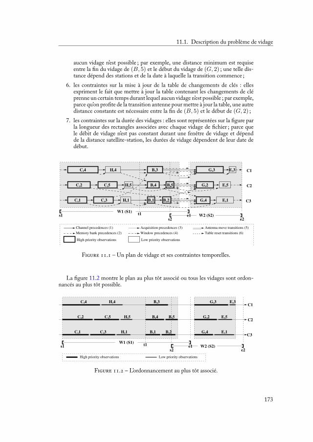
11.1. Description du problème de vidage
aucun vidage n’est possible ; par exemple, une distance minimum est requiseentre la n du vidage de (B, 5) et le début du vidage de (G, 2) ; une telle dis-tance dépend des stations et de la date à laquelle la transition commence ;
6. les contraintes sur la mise à jour de la table de changements de clés : ellesexpriment le fait que mettre à jour la table contenant les changements de cléprenne un certain temps durant lequel aucun vidage n’est possible ; par exemple,parce qu’on pro te de la transition antenne pour mettre à jour la table, une autredistance constante est nécessaire entre la n de (B, 5) et le début de (G, 2) ;
7. les contraintes sur la durée des vidages : elles sont représentées sur la gure parla longueur des rectangles associées avec chaque vidage de chier ; parce quele débit de vidage n’est pas constant durant une fenêtre de vidage et dépendde la distance satellite-station, les durées de vidage dépendent de leur date dedébut.
C1
C3
C,4
C2
C,1
C,5C,2
H,4
H,5
C,3
B,3
B,4
H,1
B,5
B,2B,1
G,2
G,4
G,3
E,5
E,1
E,3
e1s1W1 (S1)
e2s2W2 (S2)
Channel precedences (1)
Memory bank precedences (2)
t1
Window precedences (4)
Antenna move transitions (5)Acquisition precedences (3)
High priority observations Low priority observations
Table reset transitions (6)
F . – Un plan de vidage et ses contraintes temporelles.
La gure 11.2 montre le plan au plus tôt associé ou tous les vidages sont ordon-nancés au plus tôt possible.
High priority observations Low priority observations
B,3
B,1
B,5B,4C2
C3
C1E,3G,3
B,2 E,1
G,2 E,5
C,4 H,4
G,4
C,5 H,5C,2
C,3 H,1C,1
W2 (S2)e2
W1 (S1)s1
s2e1t1
F . – L’ordonnancement au plus tôt associé.
173
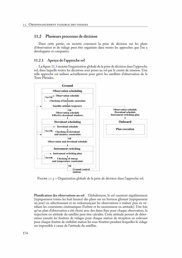
. O
11.2 Plusieurs processus de décisionDans cette partie, on montre comment la prise de décision sur les plans
d’observation et de vidage peut être organisée dans toutes les approches que l’on adéveloppées et comparées.
11.2.1 Aperçu de l’approche solLa gure 11.3 montre l’organisation globale de la prise de décision dans l’approche
sol, dans laquelle toutes les décisions sont prises au sol par le centre de mission. Unetelle approche est utilisée actuellement pour gérer les satellites d’observation de laTerre Pléiades.
Observation schedule
Observation scheduling
Checking of kinematic onstraints
Satellite attitude trajectory
OK
OK
Not OK
Not OK
Instrument switching
OK
and temperature constraints
Instrument switching plan
Instrument switching plan
Checking of energy
Observation scheduleDownload schedule
Plan execution
Ground
Observation scheduleEffective download windows
Download scheduling
Observation and download schedule
Checking of download
Download schedule
Not OK
and memory constraints
stationsGround control
Onboard
F . – Organisation globale de la prise de décision dans l’approche sol.
Plani cation des observations au sol Globalement, le sol construit régulièrement(typiquement toutes les huit heures) des plans sur un horizon glissant (typiquementun jour) en sélectionnant et en ordonnançant les observations à réaliser puis en vé-ri ant les contraintes cinématiques (l’orbite et les mouvement en attitude). Une foisqu’un plan d’observation a été choisi avec des dates xes pour chaque observation, latrajectoire en attitude du satellite peut être calculée. Cette attitude permet de déter-miner ensuite les fenêtres de vidages pour chaque station de réception en enlevantpour chaque fenêtre de visibilité station les sous-fenêtres pendant lesquelles le vidageest impossible à cause de l’attitude du satellite.
174
11.2. Plusieurs processus de décision
Plani cation des vidages au sol Le sol utilise le plan d’observation et les fenêtresde vidage effectives pour bâtir un plan de vidage sur le même horizon temporel ensélectionnant et en ordonnançant les vidages à faire et en véri ant les contraintesrelatives au vidage et à la mémoire (pas de surcharge). Pour être sûr que les plansde vidages sont exécutables, les volumes maximums sont considérés pour toutes lesobservations.
Ordonnancement de l’allumage des instruments au sol Une fois que les plansd’observation et de vidage ont été produits avec des dates de début précises pour lesobservations et les vidages, il est possible de bâtir un plan d’allumage des instruments(pour l’instrument optique et l’antenne de télémétrie) et de véri er les contraintesd’énergie et de température, ainsi que les limitations relatives aux instruments enterme de durée maximale de mise en route sur l’horizon de plani cation.
Exécution des plans à bord Une fois que tous ces plans ont été produits au sol, ilssont envoyés au satellite durant une fenêtre de visibilité de station de contrôle, etexécutés tels quels, sans aucun changement.
La première justi cation pour cette organisation de la prise de décision est qu’il estnécessaire de connaitre le plan d’observation pour construire la trajectoire en attitudedu satellite, les fenêtres de vidage effectives, et le plan de vidage, et qu’il est nécessairede connaitre le plan d’observation et de vidage pour construire le plan d’allumagedes instruments. La deuxième justi cation est qu’il a été observé dans les satellitesPléiades d’observation de la Terre actuellement en vol que les limitations en termede capacité d’observation sont dans un ordre décroissant d’impact, (1) les contraintescinématiques en attitude, (2) les contraintes relatives au vidage, (3) les contraintesrelatives à l’énergie, (4) les contraintes relatives à la température des instruments, et(5) les contraintes relatives à la mémoire de masse. Véri er d’abord les contraintes lesplus limitantes est connu comme une bonne pratique.
11.2.2 Aperçu de l’approche bordLa gure 11.4 montre l’organisation globale de la prise de décision dans l’approche
bord, dans laquelle toutes les décisions sur les vidages sont prises à bord. Cette ap-proche a été explorée dans [Pralet et al., 2014c].
Plani cation des observation au sol La plani cation des observations est réaliséeau sol dans le centre de mission exactement comme dans l’approche sol.
Ordonnancement de l’allumage des instruments au sol Parce que le sol ne sait pasquel sera le plan de vidage produit à bord, on suppose de manière pessimiste quetoutes les fenêtres de vidage seront utilisées pour le vidage. Sur cette base, il est pos-sible de bâtir un plan d’allumage des instruments et de véri er les contraintes surl’énergie et la température, ainsi que les limitations relatives aux instruments en termede durée maximale de mise en route sur l’horizon de plani cation.
Plani cation des vidages à bord Le plan d’observation et les fenêtres de vidageseffectives sont envoyés au satellite, en utilisant n’importe quelle fenêtre de visibi-lité de station de contrôle, et utilisés pour la plani cation des vidages. A bord, parce
175

. O
Observation scheduling
Observation schedule
Satellite attitude trajectory
Checking of kinematic onstraints
Not OK
OK
Ground
Not OK
Instrument switching
Instrument switching plan
and temperature constraintsChecking of energy
OK
Ground controlstations
Observation schedule
Observation scheduleEffective download windowsInstrument switching plan
Download scheduling
Download schedule
download constraintsChecking ofNot OK
OK
Observation execution
Checking ofmemory constraints
Download execution
Execution of theprecedence graph
Download precedence graph
Onboard
F . – Organisation globale de la prise de décision dans l’approche bord.
que l’information à propos des volumes arrive au moment où les observations se ter-minent, la plani cation des vidages est réalisée avant chaque groupe de fenêtres de vi-dage se chevauchant (au dernier moment, pour pro ter du maximum d’informationsconcernant les volumes), avec ce groupe de fenêtres comme horizon de plani cation.Deux fenêtres de vidage sont considérées comme se chevauchant si et seulement sielles se chevauchent temporellement ou s’il n’y a pas assez de temps entre la n dela première et le début de la seconde pour replani er les vidages. Les volumes exactssont considérés pour toutes les observations qui sont terminées au moment de la pla-ni cation et les volumes maximums pour celles qui vont nir entre le début de laplani cation et la n de l’horizon de plani cation, cela pour garantir que le plan estexécutable et n’aura pas besoin de modi cations en ligne.
Exécution des plans d’observation et d’allumage à bord Les observations sont réa-lisées et les instruments sont allumés selon le plan d’allumage produit au sol. Ce-pendant, parce que les contraintes sur la mémoire n’ont pas pu être véri ées au sol(puisque le plan de vidage est produit à bord), un mécanisme simple est utilisé à bordlors de l’exécution des observations pour éviter le dépassement de la capacité mémoireet l’écrasement de données : si la réalisation de l’observation o peut mener à un écra-sement mémoire, soit o n’est pas réalisée, soit une observation de plus faible prioritéest effacée de la mémoire pour libérer de l’espace.
Exécution du plan de vidage à bord Les vidages sont exécutés tels que spéci és parles plans de vidage, au cours des groupes de fenêtres de vidage successifs. Cependant,pour prendre en compte l’incertitude restante concernant le volume des données pro-duit par les observations qui vont nir entre le début de la plani cation des vidages etla n de l’horizon de plani cation, le plan de vidage envoyé pour exécution n’est pasxe, mais reste temporellement exible. Concrètement, ces plans ont la forme d’un
graphe de précédence (graphe orienté acyclique) dans lequel chaque nœud est exécutédès que tous ses prédécesseurs ont été exécutés. Cela permet de pro ter des vidagesdont la durée est strictement plus petite que la durée maximum qui a été considéréelors de la plani cation et ainsi de commencer les vidages plus tôt que prévu dans leplan pessimiste.
176

11.2. Plusieurs processus de décision
Garder la plani cation des observations au sol est justi é par le fait que cette pla-ni cation nécessite de nombreux calculs de mouvements en attitude du satellite : desmouvements pour passer d’une observation à une autre et des mouvements précis pourréaliser les observations avec la qualité requise. Ces mouvements sont beaucoup pluscomplexes à calculer dans le cas des satellites agiles (puisque tout le satellite doit bou-ger) que dans le cas des satellites d’ancienne génération, comme les premiers satellitesSpot (miroir mobile uniquement). Les ingénieurs considèrent que la technologie ac-tuelle ne permet pas le calcul de ces mouvements à bord. Au contraire, déporter laplani cation des vidages à bord est justi é par le fait qu’elle prend beaucoup moinsde temps que la plani cation des observations. Cette organisation est aussi justi éepar le fait que l’incertitude sur les volumes de données implique directement la plani-cation des vidages, mais seulement indirectement la plani cation des observations.
11.2.3 Aperçu de l’approche mixte sol-bordLa gure 11.5 montre l’organisation de la prise de décision dans l’approche mixte
sol-bord, principale contribution de ce chapitre, dans laquelle les décisions à proposdes vidages sont partagées entre le sol et le bord.
Observation execution
Checking ofmemory constraints
Observation schedule
Observation scheduling
Checking of kinematic onstraints
Satellite attitude trajectory
OK
OK
Not OK
Not OK
Instrument switching
OK
and temperature constraints
Instrument switching plan
Ground
Checking of energy
Observation scheduleEffective download windows
Download scheduling
Observation and download schedule
Checking of download
Download schedule
Not OK
and memory constraints
stationsGround control
Download execution
OK
precedence graphExecution of the
adaptation
Download precedence graph
Download schedule
Download schedule
download constraintsChecking of
Not OK
and commitments
Commitments
Instrument switching plan
Effective download windowsDownload schedule
Onboard
Observation schedule
Maximum resource consumption levels
F . – Organisation de la prise de décision dans l’approche mixte sol-bord.
Avec chaque observation, est associé un niveau de priorité dé ni par un entierentre 1 et Np, avec 1 la plus haute priorité et Np la plus basse. Dans la suite, on sedésigne par observation de haute priorité les observations de priorité 1 et observationde basse priorité toutes les autres, c’est à dire celles dont le niveau de priorité est plusgrand ou égal à 2.
Plani cation des observations au sol La plani cation des observations est réaliséeau sol dans le centre de mission comme dans les deux approches précédentes.
177
. O
Plani cation des vidages au sol Le sol utilise le plan d’observation et les fenêtres devidage effectives pour bâtir un plan de vidage sur le même horizon de plani cationen sélectionnant et en ordonnançant les vidages à faire et en véri ant les contraintesconcernant le vidage et la mémoire, comme c’est fait dans l’approche sol. La seule dif-férence est que les volumes maximums sont utilisés seulement pour les acquisitionsde haute priorité, de manière à garantir qu’elles pourront être vidées. Pour les acqui-sitions de basse priorité, pour lesquelles le même genre de garantie n’est pas requis,seuls les volumes espérés sont considérés. Avec chaque acquisition de haute prioritéo, on associe un engagement de type 1 ou 2 dé ni par l’utilisateur qui a demandé o.Un engagement de type 1 associé avec une observation signi e que celle-ci doit êtrevidée durant la fenêtre de vidage décidée au sol. En d’autres termes, le vidage peutseulement être avancé durant la même fenêtre. Un engagement de type 2 signi e quel’observation doit être vidée dans la fenêtre décidée au sol ou plus tôt, possiblementdans une fenêtre de vidage antérieure.
Plani cation de l’allumage des instruments au sol Parce que le sol ne sait pas quelsera le plan de vidage produit à bord (puisqu’il sera adapté à bord), on suppose demanière pessimiste que toutes les fenêtres de vidage seront utilisées pour le vidage(même supposition que dans l’approche bord). Sur cette base, il est possible de bâtirun plan d’allumage des instruments et de véri er les contraintes sur l’énergie et latempérature, ainsi que les limitations relatives aux instruments en terme de duréemaximale de mise en route sur l’horizon de plani cation.
Adaptation du plan de vidage à bord Le plan d’observation, les fenêtres de vidageseffectives, le plan de vidage (avec les engagements attachés aux acquisitions de hautepriorité), et le plan d’allumage des instruments sont envoyés au satellite comme pré-cédemment. Ces éléments sont utilisés pour l’adaptation du plan de vidage à bord.Comme dans l’approche bord, cette adaptation est réalisée avant chaque groupe defenêtres de vidage se chevauchant avec ce groupe comme horizon de plani cation.Les volumes exacts sont considérés pour toutes les observations qui sont terminéesau début de la plani cation et les volumes maximums sont considérés pour les ob-servations qui se termineront d’ici la n de l’horizon. La seule différence est que laplani cation ne se fait pas à partir de rien mais utilise le plan produit au sol. Ellel’adapte tout en garantissant les engagements relatifs aux acquisitions de haute prio-rité.
L’algorithme que nous proposons est chronologique et glouton, il construit unplan exécutable en suivant au maximum le plan de vidage produit en sol. Il le modi eparfois, (1) en avançant des acquisitions ou en insérant des acquisitions supplémen-taires non présentes dans le plan quand des volumes plus faibles que prévus créent desespaces vides dans le plan, ou (2) en supprimant des vidages qui mettent en danger laréalisation des engagements des vidages liés à des acquisitions de haute priorité. Lavéri cation à bord de la faisabilité des engagements après modi cation étant une opé-ration potentiellement couteuse en temps, des bornes majorantes sur les ressourcessont pré-calculées au sol et permettent des véri cations très rapides à bord.
Exécution des plans à bord Les plans d’observation, d’allumage, et de vidage sontexécutés à bord exactement comme dans l’approche bord précédemment présentée.
Figure 11.6 offre une autre vision de la façon dont la prise de décision est organiséetemporellement entre le sol et le bord dans l’approche mixte sol-bord.
178

11.3. Expérimentations
downloads
download
observation
observations
scheduleadaptation Satellite
data acknowledgementsinstrument switching plan
commitmentsdownload schedule
effective download windowsobservation schedule
execution
observation data
and downloadGround
satellite control data downloadobservation
scheduling
executiondownload
window window
maximum resource consumption levels
F . – Aperçu dont la prise de décision est organisée temporellement entrele sol et le bord dans l’approche mixte sol-bord.
La première justi cation de cette organisation de la prise de décision par rapportà la précédente est que, bien que la plani cation des vidages prenne bien moins detemps que la plani cation des observations, elle reste onéreuse si on considère lesressources de calcul très limitées à bord. Cela peut être une bonne idée de pro terdes ressources de calcul disponibles au sol pour bâtir des plans de vidage de qualitéet d’utiliser de simples règles de décision pour les adapter à bord. Ces plans sontproduits en considérant les volumes maximums pour les acquisitions de haute prioritépour garantir leur vidage, et les volumes espérés pour les acquisitions de basse prioritéavec l’idée que les volumes plus importants que les volumes prévus seront compenséspar les volumes moins importants que prévus (voir [Bon etti et al., 2014] pour uneétude théorique et empirique de ce phénomène). La seconde justi cation est quecette organisation augmente la prévisibilité du système, pour les observations de hautepriorité en tout cas : pour chacune d’elles, l’utilisateur sait dans quelle fenêtre ou dansquelle fenêtre au plus tard elle sera vidée.
11.3 Expérimentations
11.3.1 Approches à comparerPour apprécier l’impact positif d’un partage de la prise de décision entre le sol et
le bord, nous avons implémenté et comparé les quatre approches suivantes dans unsimulateur de satellite (présenté en anglais en Annexe A) :
1. plani cation au sol (Ground) : la plani cation des vidages est réalisée ausol à partir des volumes maximums pour toutes les observations, en utili-sant un algorithme de type SWO reposant sur un algorithme glouton non-chronologique (décrit en anglais en Section 5.3) ; ce plan est ensuite exécutéà bord ; la seule différence avec l’approche actuellement en utilisation dans lesopérations et que le graphe acyclique à bord permet une certaine exibilitétemporelle et permet à certains vidages de commencer plus tôt que dans le planpessimiste du sol (décrit en anglais en Section 6.4) ; ce dernier mécanisme joue
179
. O
plutôt en faveur de l’approche sol en terme d’age de l’information par rapportà la réalité ;
2. plani cation à bord (Board) : la plani cation des vidages est réalisée à bord àpartir de rien avant chaque groupe de fenêtres de vidage se chevauchant avecles volumes exacts pour les observations étant déjà terminées et les volumesmaximums pour les autres, en utilisant un algorithme glouton chronologique(comme décrit en anglais en Section 5.2.2) ; comme dans l’approche précé-dente, un graphe acyclique permet une certaine exibilité temporelle ;
3. la plani cation des vidages est réalisée au sol avec les volumes maximums pourles observations de haute priorité et les volumes espérés pour les autres, en utili-sant un algorithme SWO, comme dans l’approche sol ; ensuite, la plani cationest réalisée à bord avant chaque groupe de fenêtres se chevauchant avec les vo-lumes exacts pour les observations déjà terminées et les volumes maximumspour les autres, en suivant et en adaptant le plan du sol (comme décrit pré-cisément en anglais en Section 6.3) ; comme dans les approches précédentes,un graphe acyclique est construit et permet une certaine exibilité temporelle ;deux variantes du mécanisme d’adaptation à bord ont été implémentées :
a) un mécanisme d’adaptation très simple (SimpleRepair) : les vidages den’importe quelle priorité sont supprimés du plan sol s’ils sont physique-ment infaisables ; cela signi e que seules les contraintes physiques sontprises en compte ; les engagements vis-à-vis des observations de hautepriorité ne sont pas considérés ;
b) un mécanisme d’adaptation intelligent (SmartRepair) : les vidages debasse priorité sont supprimés du plan sol soit quand ils sont physique-ment infaisables, soit quand ils empêchent les vidages de haute prioritéfuturs ; des vidages sont ajoutés ou avancés quand c’est possible ; cela veutdire que les engagements, ainsi que les contraintes physiques, sont tou-jours considérés ; pour véri er que les engagements seront tenus, un mé-canisme de recherche en avant est utilisé (voir Section 6.3 en anglais pourdes détails).
11.3.2 ScénariosOn utilise deux scénarios réalistes fournis par Airbus Defence and Space. Les deux
scénarios sont produits à partir du même plan d’observation de un jour qui a été faitpour un satellite d’observation de la Terre actuellement opérationnel (environ 14 révo-lutions autour de la Terre au cours de la journée). Ils diffèrent par rapport au nombrede stations sol disponibles pour le vidage : le scénario 1 (le moins contraint) impliqueun nombre important de stations sol de réception (23) résultant dans de nombreusesfenêtres de vidage (115), tandis que le scénario 2 (le plus contraint) implique un pe-tit nombre de stations de réception (3) résultant en un petit nombre de fenêtres devidage (20). Ils diffèrent aussi dans la distribution des observations parmi les utili-sateurs et les niveaux de priorité : 275 (resp. 247) observations de haute priorité et1089 (resp. 1117) observations de basse priorité pour le scénario 1 (resp. 2). Les vo-lumes réels des chiers sont générés de façon aléatoire dans l’intervalle compris entreVmax/4 et Vmax, avec Vmax le volume maximum d’un chier. 15 instances desvolumes réels ont été générées et tous les résultats sont des valeurs moyennes sur ces15 instances. Les expérimentations on été réalisées avec un processeur Xeon 4-coeurs3GHz avec 8GB RAM, sur Ubuntu 12.04 LTS.
180
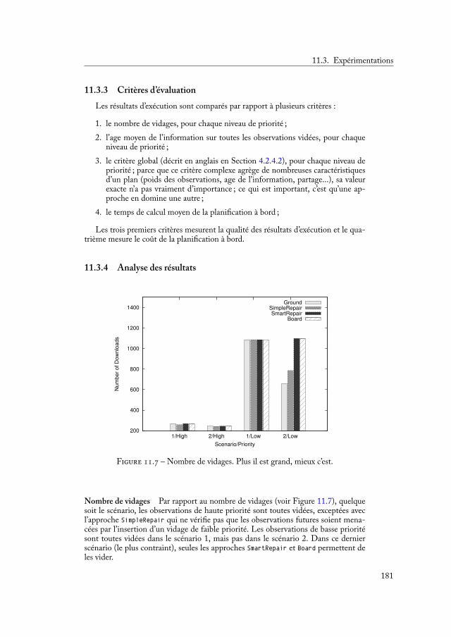
11.3. Expérimentations
11.3.3 Critères d’évaluationLes résultats d’exécution sont comparés par rapport à plusieurs critères :
1. le nombre de vidages, pour chaque niveau de priorité ;2. l’age moyen de l’information sur toutes les observations vidées, pour chaque
niveau de priorité ;3. le critère global (décrit en anglais en Section 4.2.4.2), pour chaque niveau de
priorité ; parce que ce critère complexe agrège de nombreuses caractéristiquesd’un plan (poids des observations, age de l’information, partage...), sa valeurexacte n’a pas vraiment d’importance ; ce qui est important, c’est qu’une ap-proche en domine une autre ;
4. le temps de calcul moyen de la plani cation à bord ;
Les trois premiers critères mesurent la qualité des résultats d’exécution et le qua-trième mesure le coût de la plani cation à bord.
11.3.4 Analyse des résultats
200
400
600
800
1000
1200
1400
1/High 2/High 1/Low 2/Low
NumberofDownloads
Scenario/Priority
GroundSimpleRepairSmartRepair
Board
F . – Nombre de vidages. Plus il est grand, mieux c’est.
Nombre de vidages Par rapport au nombre de vidages (voir Figure 11.7), quelquesoit le scénario, les observations de haute priorité sont toutes vidées, exceptées avecl’approche SimpleRepair qui ne véri e pas que les observations futures soient mena-cées par l’insertion d’un vidage de faible priorité. Les observations de basse prioritésont toutes vidées dans le scénario 1, mais pas dans le scénario 2. Dans ce dernierscénario (le plus contraint), seules les approches SmartRepair et Board permettent deles vider.
181

. O
5000
10000
15000
20000
25000
30000
35000
1/High 2/High 1/Low 2/Low
MeanInform
ationAge(s)
Scenario/Priority
GroundSimpleRepairSmartRepair
Board
F . – Age moyen de l’information (en secondes). Plus il est petit, mieuxc’est.
Age moyen de l’information Des différences importantes apparaissent sur la Fi-gure 11.8, mais seulement pour les observations de basse priorité sur le scénario 2(le plus contraint). L’age moyen de l’information diminue à mesure que la prise dedécision est déportée à bord.
0.0001
0.001
0.01
0.1
1
1/High 2/High 1/Low 2/Low
Crite
rio
n
Scenario/Priority
GroundSimpleRepairSmartRepair
Board
F . – Critère global (sur une échelle logarithmique). Plus il est grand, mieuxc’est.
Critère global Par rapport au critère global, la Figure 11.9 montre que, pour lesobservations de haute priorité sur le scénario 1, les approches Ground et SmartRepair
182

11.3. Expérimentations
sont meilleures que les approches SimpleRepair et Board. Pour l’approche SimpleRe-pair, cela peut être expliqué par le fait que l’algorithme d’adaptation supprime desvidages de haute priorité. Pour l’approche Board, cela peut être expliqué par le fait queles plani cations bord sont effectuées successivement sur des horizons très limités,tandis que les approches Ground et SmartRepair travaillent sur un grand horizon de pla-ni cation et optimisent explicitement le critère global avec l’algorithme SWO. Pourles observations de basse priorité, l’approche SmartRepair est clairement supérieuresur le scénario 2, suggérant l’impact positif d’une combinaison entre un algorithmed’optimisation au sol sur un large horizon et une adaptation du plan à bord sur despetits horizons successifs.
0.01
0.02
0.03
0.04
0.05
0.06
0.07
0.08
0.09
0.1
1 2
MeanComputingTimeOnboard(s)
Scenario
GroundSimpleRepairSmartRepair
Board
F . – Temps moyen de calcul à bord. Plus il est petit, mieux c’est.
Temps moyen de calcul à bord Sans surprise, les résultats sur la Figure 11.10montrent que plus la prise de décision est déportée à bord, plus le temps moyen decalcul à bord est important (ce temps est trop faible pour être montré pour l’approcheGround). Signalons que l’approche SmartRepair est capable d’obtenir des résultats si-milaires ou supérieurs en terme de nombre de vidages, d’age de l’information, et decritère global, par rapport à l’approche bord avec 1.5 à 3 fois moins de temps de calculà bord.
183

Plani cation exible des acquisitions 12
12.1 Quelques choix de conception . . . . . . . . . . . . . . . . 18412.2 Production d’un plan d’observation conditionnel au sol . . . . 18412.3 Exécution d’un plan d’observation conditionnel à bord . . . . 18712.4 Expérimentations . . . . . . . . . . . . . . . . . . . . . . . 188
12.4.1 Approches à comparer . . . . . . . . . . . . . . . . 18812.4.2 Scenarios . . . . . . . . . . . . . . . . . . . . . . 18812.4.3 Résultats . . . . . . . . . . . . . . . . . . . . . . . 189
Nous avons aussi examiné le problème de plani cation des acquisitions quiconsiste à sélectionner et ordonnancer les observations que le satellite réalisera 1. Denos jours, les plans d’observation sont produits au sol. Un plan de vidage est ensuiteconstruit et le tout est simulé pour véri er que les contraintes sur l’énergie, la tem-pérature et la mémoire sont bien respectées par le plan. Si certaines contraintes sontviolées, des acquisitions de faible priorité sont supprimées du plan d’observation et devidage et le processus de simulation est relancé. Parce que la simulation de l’évolutionde l’énergie ou de la température est une opération nécessitant de fortes ressourcesde calcul, cela ne peut pas être fait nement durant la plani cation. Cette simulationne est donc remplacée par des contraintes de haut niveau ajoutées au problème. Ces
contraintes sont très margées par rapport à la réalité pour assurer la sûreté du satel-lite. Les paramètres affectés par ces marges sont la consommation et la productiond’énergie, l’évolution de la température et le volumes des observations. La consom-mation d’énergie réelle est souvent moins importante que celle prévue par les marges,la production d’énergie réelle est souvent plus importante que celle prévue par lesmarges, et ainsi de suite. Le pro l d’énergie est donc toujours plus haut que prévu etpourtant, un nombre important d’acquisitions qui auraient pu être réalisées et vidéessont éliminées de la plani cation à cause des contraintes de haut niveau. Pour amé-liorer la capacité du système, l’idée développée ici est de supprimer ces contraintes dehaut niveau pour les acquisitions de faible priorité. Cependant, et contrairement auproblème de vidage, il n’est pas possible d’adapter les plans à bord à cause des faiblescapacités de calcul disponibles à bord et de la difficulté d’adaptation qui est plus beau-coup grande. Cela signi e que le bord peut seulement exécuter les plans. Dans unenouvelle approche, les plans d’observation produits au sol sont des plans condition-nels contenant des conditions pour déclencher les acquisitions de faible priorité. Bâtirces plans conditionnels implique le remplacement des contraintes de haut niveau parun mécanisme dans lequel on calcule d’abord les niveaux minimums d’énergie de-vant être présents à bord au début de chaque acquisition de faible priorité de manièreà assurer que si on réalise cette acquisition, toutes les futures acquisitions de hautepriorité pourront être effectuées. Ces niveaux sont produits grâce à une procédurede simulation à rebours qui commence à la n de l’horizon et qui calcule des bornesde réalisation sur les niveaux d’énergie. Une fois à bord, avant chaque acquisition defaible priorité, si le niveau d’énergie réel est plus important que le niveau requis calculéau sol, l’acquisition est réalisée. Sinon, l’instrument d’observation n’est pas allumé et
1. Cette partie du travail a été présentée au IJCAI’15 International Workshop on Planning & Schedulingfor Space (IWPSS’15) [Maillard et al., 2015b].
185
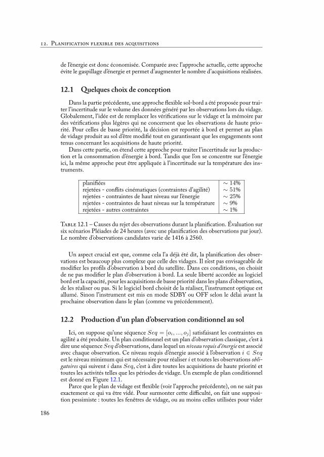
. P
de l’énergie est donc économisée. Comparée avec l’approche actuelle, cette approcheévite le gaspillage d’énergie et permet d’augmenter le nombre d’acquisitions réalisées.
12.1 Quelques choix de conceptionDans la partie précédente, une approche exible sol-bord a été proposée pour trai-
ter l’incertitude sur le volume des données généré par les observations lors du vidage.Globalement, l’idée est de remplacer les véri cations sur le vidage et la mémoire pardes véri cations plus légères qui ne concernent que les observations de haute prio-rité. Pour celles de basse priorité, la décision est reportée à bord et permet au plande vidage produit au sol d’être modi é tout en garantissant que les engagements sonttenus concernant les acquisitions de haute priorité.
Dans cette partie, on étend cette approche pour traiter l’incertitude sur la produc-tion et la consommation d’énergie à bord. Tandis que l’on se concentre sur l’énergieici, la même approche peut être appliquée à l’incertitude sur la température des ins-truments.
plani ées ∼ 14%rejetées - con its cinématiques (contraintes d’agilité) ∼ 51%rejetées - contraintes de haut niveau sur l’énergie ∼ 25%rejetées - contraintes de haut niveau sur la température ∼ 9%rejetées - autres contraintes ∼ 1%
T 12.1 – Causes du rejet des observations durant la plani cation. Évaluation sursix scénarios Pléiades de 24 heures (avec une plani cation des observations par jour).Le nombre d’observations candidates varie de 1416 à 2560.
Un aspect crucial est que, comme cela l’a déjà été dit, la plani cation des obser-vations est beaucoup plus complexe que celle des vidages. Il n’est pas envisageable demodi er les pro ls d’observation à bord du satellite. Dans ces conditions, on choisitde ne pas modi er le plan d’observation à bord. La seule liberté accordée au logicielbord est la capacité, pour les acquisitions de basse priorité dans les plans d’observation,de les réaliser ou pas. Si le logiciel bord choisit de la réaliser, l’instrument optique estallumé. Sinon l’instrument est mis en mode SDBY ou OFF selon le délai avant laprochaine observation dans le plan (comme vu précédemment).
12.2 Production d’un plan d’observation conditionnel au solIci, on suppose qu’une séquence Seq = [oi, ..., oj ] satisfaisant les contraintes en
agilité a été produite. Un plan conditionnel est un plan d’observation classique, c’est àdire une séquence Seq d’observations, dans lequel un niveau requis d’énergie est associéavec chaque observation. Ce niveau requis d’énergie associé à l’observation i ∈ Seqest le niveau minimum qui est nécessaire pour réaliser i et toutes les observations obli-gatoires qui suivent i dans Seq, c’est à dire toutes les acquisitions de haute priorité ettoutes les activités telles que les périodes de vidage. Un exemple de plan conditionnelest donné en Figure 12.1.
Parce que le plan de vidage est exible (voir l’approche précédente), on ne sait pasexactement ce qui va être vidé. Pour surmonter cette difficulté, on fait une supposi-tion pessimiste : toutes les fenêtres de vidage, ou au moins celles utilisées pour vider
186
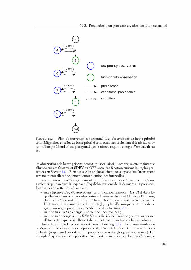
12.2. Production d’un plan d’observation conditionnel au sol
F . – Plan d’observation conditionnel. Les observations de haute prioritésont obligatoires et celles de basse priorité sont exécutées seulement si le niveau cou-rant d’énergie à bord E est plus grand que le niveau requis d’énergie Ren calculé ausol.
les observations de haute priorité, seront utilisées ; ainsi, l’antenne va être maintenueallumée sur ces fenêtres et SDBY ou OFF entre ces fenêtres, suivant les règles pré-sentées en Section12.1. Bien sûr, si elles se chevauchent, on suppose que l’instrumentsera maintenu allumé seulement durant l’union des intervalles.
Les niveaux requis d’énergie peuvent être efficacement calculés par une procédureà rebours qui parcourt la séquence Seq d’observations de la dernière à la première.Les entrées de cette procédure sont :
– une séquence Seq d’observations sur un horizon temporel [Hs, He] dans la-quelle nous ajoutons deux observations ctives au début et à la n de l’horizon,dont la durée est nulle et la priorité haute ; les observations dans Seq, ainsi queles ctives, sont numérotées de 1 à |Seq| ; le plan d’allumage peut être calculégrâce aux règles présentées précédemment en Section12.1 ;
– un niveau EnHs d’énergie au début de l’horizon Hs ;– un niveau d’énergie requis REnHe à la n He de l’horizon ; ce niveau permet
d’être certain que le satellite est dans un état sûr pour les prochaines orbites.Une exécution de la procédure est présenté en Fig 12.2. Un sous-ensemble de
la séquence d’observations est réprésenté de l’Acq. 4 à l’Acq. 9. Les observationsde haute (resp. basse) priorité sont représentées en rectangles gras (resp. mince). Parexemple Acq. 8 est de haute priorité et Acq. 9 est de basse priorité. Le plan d’allumage
187
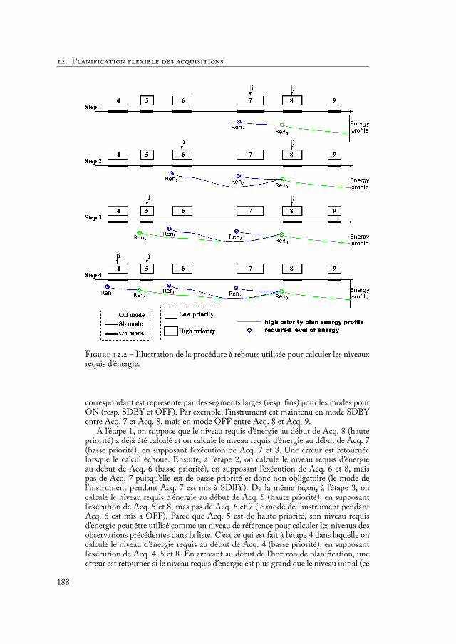
. P
F . – Illustration de la procédure à rebours utilisée pour calculer les niveauxrequis d’énergie.
correspondant est représenté par des segments larges (resp. ns) pour les modes pourON (resp. SDBY et OFF). Par exemple, l’instrument est maintenu en mode SDBYentre Acq. 7 et Acq. 8, mais en mode OFF entre Acq. 8 et Acq. 9.
A l’étape 1, on suppose que le niveau requis d’énergie au début de Acq. 8 (hautepriorité) a déjà été calculé et on calcule le niveau requis d’énergie au début de Acq. 7(basse priorité), en supposant l’exécution de Acq. 7 et 8. Une erreur est retournéelorsque le calcul échoue. Ensuite, à l’étape 2, on calcule le niveau requis d’énergieau début de Acq. 6 (basse priorité), en supposant l’exécution de Acq. 6 et 8, maispas de Acq. 7 puisqu’elle est de basse priorité et donc non obligatoire (le mode del’instrument pendant Acq. 7 est mis à SDBY). De la même façon, à l’étape 3, oncalcule le niveau requis d’énergie au début de Acq. 5 (haute priorité), en supposantl’exécution de Acq. 5 et 8, mas pas de Acq. 6 et 7 (le mode de l’instrument pendantAcq. 6 est mis à OFF). Parce que Acq. 5 est de haute priorité, son niveau requisd’énergie peut être utilisé comme un niveau de référence pour calculer les niveaux desobservations précédentes dans la liste. C’est ce qui est fait à l’étape 4 dans laquelle oncalcule le niveau d’énergie requis au début de Acq. 4 (basse priorité), en supposantl’exécution de Acq. 4, 5 et 8. En arrivant au début de l’horizon de plani cation, uneerreur est retournée si le niveau requis d’énergie est plus grand que le niveau initial (ce
188

12.3. Exécution d’un plan d’observation conditionnel à bord
qui voudrait dire que le plan est infaisable). Sinon, l’algorithme termine correctement.
12.3 Exécution d’un plan d’observation conditionnel à bord
A bord, toutes les acquisitions de haute priorité sont exécutées. Avant chaqueacquisition de basse priorité i, si le niveau d’énergie à bord et plus grand ou égalau niveau requis d’énergie Reni calculé au sol, l’acquisition i est réalisée. Sinon,l’instrument d’observation est mis dans le mode initialement prévu juste aprèsl’observation i pour économiser de l’énergie (voir Figure 12.3 pour un exemple).
F . – Annulation d’une observation et son effet sur l’énergie à bord. Il y aun niveau requis d’énergie pour chaque observation o1, o2, o3, o4, o5. Avant chaqueobservation de basse priorité comme o3, si le niveau d’énergie courant est plus petitque le niveau requis calculé au sol, l’observation est annulée pour assurer la réalisationdes toutes les futures acquisitions de haute priorité.
Comme dans l’approche exible pour le vidage des données, on veut que ce mé-canisme assure la réalisation des observations de haute priorité. Premièrement, sila procédure à rebours termine normalement, on est sûr que le sous-plan constituéseulement des observations de haute priorité est exécutable puisque les consomma-tions d’énergie maximum et les productions d’énergie minimum ont été utilisées pource sous-ensemble d’observations. Si l’observation oi à l’indice i est de haute priorité,il est sûr que toutes les observations de haute priorité situées après oi peuvent êtreréalisées. Maintenant, on considère une observation de basse priorité oi−1 à l’indexi− 1. Le niveau requis d’énergie pour oi−1 a été calculé en partant du niveau requispour oi et en simulant à rebours depuis oi jusqu’au début de oi−1. Toutes les fenêtresde vidages ont été prises en compte. Alors si le niveau d’énergie à bord est plus grandque Reni−1 au début de oi−1, on est sûr qu’il est plus grand que Reni au début deoi. Alors, toutes les observations de haute priorité futures peuvent être réalisées.
189
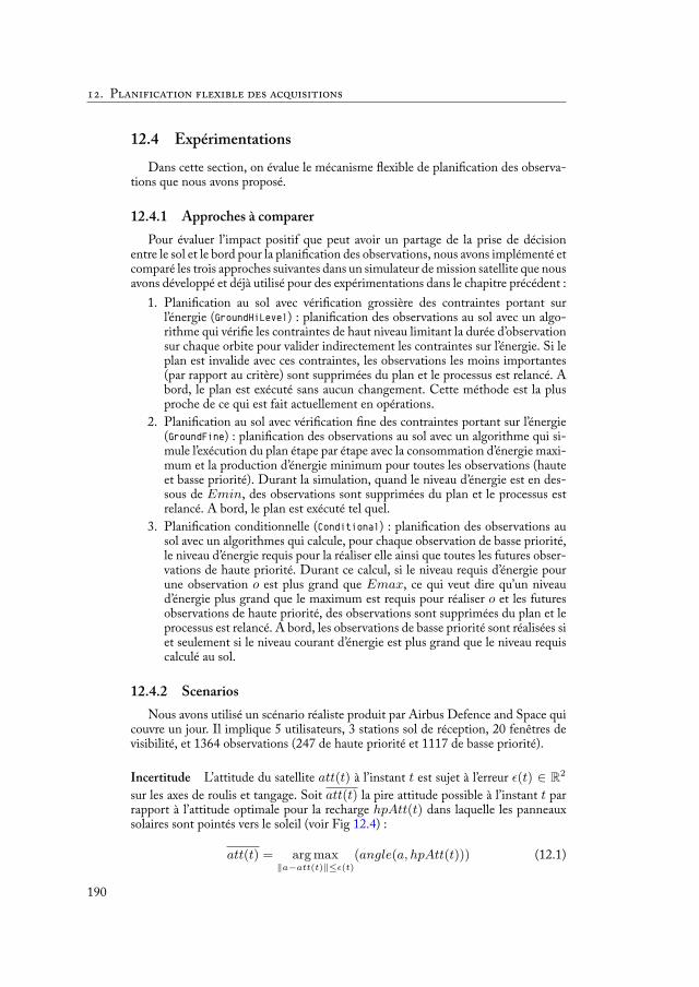
. P
12.4 ExpérimentationsDans cette section, on évalue le mécanisme exible de plani cation des observa-
tions que nous avons proposé.
12.4.1 Approches à comparerPour évaluer l’impact positif que peut avoir un partage de la prise de décision
entre le sol et le bord pour la plani cation des observations, nous avons implémenté etcomparé les trois approches suivantes dans un simulateur de mission satellite que nousavons développé et déjà utilisé pour des expérimentations dans le chapitre précédent :
1. Plani cation au sol avec véri cation grossière des contraintes portant surl’énergie (GroundHiLevel) : plani cation des observations au sol avec un algo-rithme qui véri e les contraintes de haut niveau limitant la durée d’observationsur chaque orbite pour valider indirectement les contraintes sur l’énergie. Si leplan est invalide avec ces contraintes, les observations les moins importantes(par rapport au critère) sont supprimées du plan et le processus est relancé. Abord, le plan est exécuté sans aucun changement. Cette méthode est la plusproche de ce qui est fait actuellement en opérations.
2. Plani cation au sol avec véri cation ne des contraintes portant sur l’énergie(GroundFine) : plani cation des observations au sol avec un algorithme qui si-mule l’exécution du plan étape par étape avec la consommation d’énergie maxi-mum et la production d’énergie minimum pour toutes les observations (hauteet basse priorité). Durant la simulation, quand le niveau d’énergie est en des-sous de Emin, des observations sont supprimées du plan et le processus estrelancé. A bord, le plan est exécuté tel quel.
3. Plani cation conditionnelle (Conditional) : plani cation des observations ausol avec un algorithmes qui calcule, pour chaque observation de basse priorité,le niveau d’énergie requis pour la réaliser elle ainsi que toutes les futures obser-vations de haute priorité. Durant ce calcul, si le niveau requis d’énergie pourune observation o est plus grand que Emax, ce qui veut dire qu’un niveaud’énergie plus grand que le maximum est requis pour réaliser o et les futuresobservations de haute priorité, des observations sont supprimées du plan et leprocessus est relancé. A bord, les observations de basse priorité sont réalisées siet seulement si le niveau courant d’énergie est plus grand que le niveau requiscalculé au sol.
12.4.2 ScenariosNous avons utilisé un scénario réaliste produit par Airbus Defence and Space qui
couvre un jour. Il implique 5 utilisateurs, 3 stations sol de réception, 20 fenêtres devisibilité, et 1364 observations (247 de haute priorité et 1117 de basse priorité).
Incertitude L’attitude du satellite att(t) à l’instant t est sujet à l’erreur ϵ(t) ∈ R2
sur les axes de roulis et tangage. Soit att(t) la pire attitude possible à l’instant t parrapport à l’attitude optimale pour la recharge hpAtt(t) dans laquelle les panneauxsolaires sont pointés vers le soleil (voir Fig 12.4) :
att(t) = arg max∥a−att(t)∥≤ϵ(t)
(angle(a, hpAtt(t))) (12.1)
190
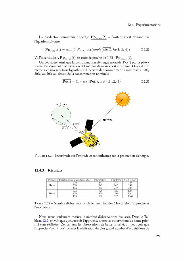
12.4. Expérimentations
La production minimum d’énergie Ppsolar(t) à l’instant t est donnée parl’équation suivante :
Ppsolar(t) = max(0, Psun · cos(angle(att(t), hpAtt(t)))) (12.2)
Vu l’incertitude ϵ, Ppsolar(t) est estimée proche de 0.75 ·Ppsolar(t).On considère aussi que la consommation d’énergie normale Pc(t) par la plate-
forme, l’instrument d’observation et l’antenne d’émission est incertaine. On évalue lemême scénario avec trois hypothèses d’incertitude : consommation maximale à 10%,20%, ou 30% au-dessus de la consommation nominale :
Pc(t) = (1 + α) ·Pc(t), α ∈ .1, .2, .3 (12.3)
F . – Incertitude sur l’attitude et son in uence sur la production d’énergie.
12.4.3 Résultats
Priorité Incertitude sur la production (α) GroundHiLevel GroundFine Conditional
Haute10% 247 247 24720% 247 247 24730% 247 247 247
Basse10% 976 1053 108620% 938 1010 106130% 898 927 1040
T 12.2 – Nombre d’observations réellement réalisées à bord selon l’approche etl’incertitude.
Nous avons seulement mesuré le nombre d’observations réalisées. Dans le Ta-bleau 12.2, on voit que quelque soit l’approche, toutes les observations de haute prio-rité sont réalisées. Concernant les observations de basse priorité, on peut voir quel’approche Conditional permet la réalisation du plus grand nombre d’acquisitions de
191

. P
basse priorité. Sans surprise, l’approche GroundFine qui simule nement le pro l enénergie est plus efficace et permet la réalisation de plus d’observations de basse prio-rité que l’approche GroundHiLevel qui valide les contraintes de haut niveau seulement.De plus, on peut voir que plus l’incertitude est grande sur la production et la consom-mation d’énergie, plus l’approche conditionnelle est intéressante.
La Figure 12.5 montre le niveau d’énergie à bord durant l’exécution d’un scéna-rio de 24 heures à travers différentes perspectives. La méthode GroundFine calculed’abord un pro l en énergie simulé (pointillés sur la gure) en se basant sur les piresproductions et consommations d’énergie. Une procédure supprime des observationjusqu’à ce que ce pro l ne passe plus en-dessous de Emin, c’est à dire 85% de Emaxdans ce cas. On peut voir que le pro l prédit et le pro l réel produit par l’approcheConditional sont assez proches au début et à la n du jour parce que les activitésd’observation et de vidage sont réalisées principalement entre 6 heures et 18 heures.On peut aussi con rmer que le niveau d’énergie à bord ne tombe jamais en dessousdu niveau minimum Emin durant l’exécution du plan conditionnel.
75
80
85
90
95
100
20:00 00:00 04:00 08:00 12:00 16:00 20:00 00:00
Ener
gy (%
)
Time (hours)
Energy available on board on a 1-day scenario
realrequired
predicted
F . – Niveau d’énergie à bord au cours d’un scénario de 24 heures.
Cette évaluation a été réalisées en utilisant un seul scénario, il aurait été intéressantde montrer la robustesse de l’approche sur d’autres scénarios réalistes et avec d’autresparamètres physiques. Les expérimentations ont été faites sur un processeur Xeon4-coeur 3GHz avec 8GB RAM, sur Ubuntu 12.04 LTS.
192
Perspectives 13
Dans ce manuscrit, nous avons tenté de montrer les propriétés et les avantagesd’un mécanisme de prise de décision qui serait partagé entre le sol et le bord pour unsatellite agile d’observation de la Terre. On décrit maintenant quelques perspectives.
Problème de plani cation du vidage des observations– Des algorithmes d’approximation sont utilisées pour produire des plans de vi-
dages, tels que l’algorithme de type SWO. Il serait intéressant de comparerla qualité des solutions trouvées avec les solutions optimales. Cela parait biendifficile de calculer ces solutions optimales dans le cas des scénarios réalistes.Il y a pourtant deux options qui ne sont pas parfaites mais assez satisfaisantespour avoir une idée à ce propos. Une première option serait de calculer la dis-tance entre les solutions optimales et approximées sur des instances plus petitesmais suffisamment contraintes du problème. La seconde option impliquerait lesscénarios réalistes mais les approximations seraient comparés avec les solutionsoptimales sur des relaxations des sous-problèmes (comme les sous-problèmesd’allocation ou d’ordonnancement) puisque ceux-ci sont beaucoup plus simplesà résoudre séparément que lorsqu’ils sont tous intégrés.
– Nous avons utilisé un modèle d’incertitude très simpli é. Pour l’instant, nousavons supposé que les volumes réels des chiers étaient distribués de manièreuniforme sur l’intervalle d’incertitude. D’autres modèles pourraient être consi-dérés. Un modèle météo pourrait permettre une plani cation plus informéeaussi.
– Nous pourrions évaluer la plani cation exible des vidages avec de nouvellesmétriques, avec d’autres scénarios possédant une plus grande variabilité enterme de nombre de stations et de répartition des observations parmi les utili-sateurs. Par exemple, un des points qui reste à aborder est la conception d’uncritère permettant d’optimiser la exibilité d’un plan de vidage au sol.
– Des algorithmes ont été proposés pour bâtir des plans de vidage complets.Au sol, un algorithme SWO bâti au-dessus d’un glouton non-chronologiqueest utilisé. D’autre métaheuristiques pourraient être utilisées, comme les al-gorithmes génétiques par exemple. Dans le même esprit, il serait intéressantd’évaluer l’in uence des paramètres, comme la taille de l’horizon de plani -cation. Sur ce point, il est habituellement positif d’avoir un grand horizon deplani cation dans le cas déterministe. Dans le cas d’un problème avec incer-titude, il faut certainement équilibrer la taille de l’horizon de plani cation enfonction de la quantité d’incertitudes. En effet, s’il y a trop d’incertitudes surle futur, les plans deviennent vite invalides à l’exécution.
– La prise de décision lors de la phase d’exécution du plan à bord n’a pas étéencore explorée. Durant cette phase, de la exibilité temporelle est fournie parle format du plan. Une règle réactive pourrait être conçue pour prendre desdécisions pour les observations se terminant pendant cette phase. Par exemple,si une de ces observations possède un volume plus faible que prévu (plus faibleque maximum), et que l’exécution attend la n d’une autre observation, unerègle de décision peut être capable d’insérer de nouveaux vidages dans le planpour pro ter de ces espaces inutilisés.
193
. P
Problème de plani cation des observations– Un nombre plus important d’expérimentations devraient être réalisées sur une
plus large gamme de scénarios pour démontrer la viabilité de l’approche pro-posée.
– Il serait désirable de relâcher l’hypothèse que toutes les fenêtres de vidages sontutilisées pour le vidage. Tandis que cette hypothèse est proche de la réalité dansles scénarios sur-contraints, dans lesquels il y a peu de stations sol et donc peude fenêtres de vidage, l’hypothèse est bien loin de la réalité dans les scénarioscivils dans lesquels il y a de nombreuses stations couvrant tous les continents etdans lesquels les fenêtres de vidages sont sous-utilisées. Cette hypothèse rendla plani cation des vidages très pessimiste puisque il est supposé que l’antenned’émission est pratiquement toujours allumée. Une meilleure option consiste-rait à calculer au sol le niveau requis pour utiliser un groupe de fenêtres devidage. A bord, avant chacun de ces groupes, si le niveau d’énergie à nord estsuffisant, alors le groupe peut être utilisé librement pour vider des données.Sinon, seules les observations de hautes priorité seraient vidées, cela pour éco-nomiser de l’énergie.
– Des recherches futures pourraient consister à adapter le même mécanisme deplani cation conditionnelle pour traiter l’incertitude sur la température des ins-truments. Cela permettrait de relâcher les contraintes de haut niveau utiliséeslors de la plani cation, contraintes qui conduisent à rejeter 9% des observations.
– Finalement, une extension importante consisterait à calculer les pro lsd’observation à bord. Cela permettrait de rendre le satellite plus autonome etde concevoir un mécanisme de prise de décision encore plus exible, tel que ce-lui pour la plani cation des vidages. Bien qu’il ne soit pas possible de calculerces pro ls à bord pour l’instant, il serait faisable de calculer des plans avec despro ls d’attitude conditionnels (un pro l pour chaque branche du plan).
Plateforme expérimentaleUne perspective intéressante, que ce soit pour le problème de plani cation des vi-
dages ou de plani cation des observations, serait de combler le fossé entre la théorie etla pratique en menant des expérimentations sur des ordinateurs de bord. Implémen-ter ces approches représenteraient certainement un dé puisqu’ils impliquent tout lesystème sol et bord. De plus, certaines contraintes relatives aux algorithmes bord de-vraient être considérées, comme par exemple le temps de calcul et les performances.
Un cadre de prise de décision génériqueNous avons vu que la prise de décision exible peut être utilisée pour des problèmes
impliquant de larges horizons de plani cation et des incertitudes sur beaucoup detâches. Quand certaines tâches sont obligatoires, comme les observations de hautepriorité ou leurs vidages, il est possible de garantir leurs réalisations s’il est possiblede récupérer des estimations pire-cas de leurs consommations en ressources (volumesde chiers maximums, productions et consommations d’énergie maximums...). Plu-sieurs cadres existent déjà pour la décision dans l’incertain mais la mise à l’échelle serévèle souvent difficile (typiquement le cadre stochastic programming). Dans ce manus-crit, on a montré qu’il est possible de prendre en compte des problèmes complexes detaille importante. Généraliser le cadre qui a été développé pour la plani cation des ac-tivités de satellites d’observation de la Terre permettrait de traiter d’autres problèmes
194

de la même façon. Online stochastic combinatorial optimization propose un peu l’idéesimilaire qui consiste à uni er deux phases de prise de décision : une phase de dé-cision rapide en-ligne avec des méthodes habituellement utilisées hors-ligne commel’échantillonnage. Dans notre approche, le but est de spécialiser l’effort calculatoire enfonction de la phase de décision et de faciliter l’adaptation en-ligne des plans calculéshors-ligne. Finalement, nous nous concentrons plus sur les contraintes relatives auxressources et à l’idée de garantir la réalisation de certaines activités obligatoires.
195

Bibliography
P. Aguiar Melgarejo, P. Laborie, and C. Solnon. A Time-Dependent No-OverlapConstraint: Application to Urban Delivery Problems. In 12th International Con-ference on Integration of Arti cial Intelligence and Operations Research Techniques inConstraint Programming (CP-AI-OR), LNCS, pages 1–17. Springer, May 2015.
M. Ai-Chang, J. Bresina, L. Charest, A. Chase, J.-J. Hsu, A. Jonsson, B. Kanefsky,P. Morris, K. Rajan, J. Yglesias, et al. Mapgen: mixed-initiative planning andscheduling for the mars exploration rover mission. Intelligent Systems, IEEE, 19(1):8–12, 2004.
P. Auer. Using con dence bounds for exploitation-exploration trade-offs. e Journalof Machine Learning Research, 3:397–422, 2003.
P. Awasthi and T. Sandholm. Online stochastic optimization in the large: Appli-cation to kidney exchange. In Proc. of the 21st International Joint Conference onArti cial Intelligence, Pasadena, California, USA, pages 405–411, 2009.
L. Barbulescu, A. E. Howe, M. Roberts, and L. D. Whitley. Understanding Al-gorithm Performance on an Oversubscribed Scheduling Application. Journal ofArti cial Intelligence Research, 27:577–615, 2006.
R. Barták and M. A. Salido. Constraint satisfaction for planning and schedulingproblems. Constraints, 16(3):223–227, 2011.
M. Bartusch, R. H. Möhring, and F. J. Radermacher. Scheduling project networkswith resource constraints and time windows. Annals of operations Research, 16(1):199–240, 1988.
G. Beaumet, G. Verfaillie, and M. Charmeau. Estimation of the Minimal Dura-tion of an Attitude Change for an Autonomous Agile Earth-observing Satellite.In Proc. of the 13th International Conference on Principles and Practice of ConstraintProgramming (CP-07), pages 3–17, Providence, RI, USA, 2007.
G. Beaumet, G. Verfaillie, and M. Charmeau. Feasibility of Autonomous DecisionMaking on board an Agile Earth-observing Satellite. Computational Intelligence,27(1):123–139, 2011.
G. Behrmann, A. Cougnard, A. David, E. Fleury, K. G. Larsen, and D. Lime.Uppaal-tiga: Time for playing games! In Proc. of the 19th International Conferenceon Computer Aided Veri cation (CAV), pages 121–125, Berlin, Germany, 2007.
197
B
T. Benoist, B. Estellon, F. Gardi, R. Megel, and K. Nouioua. Localsolver 1.x: ablack-box local-search solver for 0-1 programming. 4OR, 9(3):299–316, 2011.
D. Bernard, G. A. Dorais, C. Fry, E. B. Gamble, B. Kanefsky, J. Kurien, W. Millar,N. Muscettola, P. Nayak, B. Pell, K. Rajan, N. Rouquette, B. Smith, and B. C.Williams. Design of the remote agent experiment for spacecraft autonomy. InAerospace Conference, volume 2, pages 259–281. IEEE, 1998.
P. Bertoli, A. Cimatti, M. Pistore, M. Roveri, and P. Traverso. Mbp: a model basedplanner. In Proc. of the IJCAI’01 Workshop on Planning under Uncertainty and In-complete Information, 2001.
J.-C. Billaut, A. Moukrim, and E. Sanlaville. Flexibility and robustness in scheduling.John Wiley & Sons, 2013.
R. Bjarnason, A. Fern, and P. Tadepalli. Lower bounding klondike solitaire withmonte-carlo planning. In Proc. of the 19th International Conference on AutomatedPlanning and Scheduling (ICAPS-09), 2009.
A. Bon etti, M. Lombardi, and M. Milano. Disregarding Duration Uncertaintyin Partial Order Schedules? Yes, We Can! In Proc. of the International Con-ference on Integration of Arti cial Intelligence and Operations Research Techniquesin Constraint Programming for Combinatorial Optimization Problems (CP-AI-OR-14), pages 210–225, Cork, Ireland, 2014.
J. Bresina, R. Dearden, N. Meuleau, S. Ramkrishnan, D. Smith, and R. Washington.Planning under Continuous Time and Resource Uncertainty: A Challenge for AI.In Proc. of the 18th International Conference on Uncertainty in Arti cial Intelligence(UAI-02), pages 77–84, Edmonton, Alberta, Canada, 2002a.
J. Bresina. Heuristic-biased stochastic sampling. In Proc. of the irteenth NationalConference on Arti cial Intelligence and Eighth Innovative Applications of Arti cialIntelligence Conference, AAAI, IAAI, Portland, Oregon, pages 271–278, 1996.
J. L. Bresina, R. Dearden, N. Meuleau, S. Ramakrishnan, D. E. Smith, andR. Washington. Planning under continuous time and resource uncertainty: Achallenge for AI. In Proc. of the 18th Conference in Uncertainty in Arti cial Intelli-gence, University of Alberta, Edmonton, Alberta, Canada, pages 77–84, 2002b.
C. B. Browne, E. Powley, D. Whitehouse, S. M. Lucas, P. I. Cowling, P. Rohlfsha-gen, S. Tavener, D. Perez, S. Samothrakis, and S. Colton. A survey of monte carlotree search methods. Computational Intelligence and AI in Games, IEEE Transac-tions on, 4(1):1–43, 2012.
R. Castano, T. Estlin, R. Anderson, D. Gaines, A. Castano, B. Bornstein,C. Chouinard, and M. Judd. OASIS: Onboard Autonomous Science Investi-gation System for Opportunistic Rover Science. Journal of Field Robotics, 24(5):379–397, 2007.
A. Cesta, G. Cortellessa, S. Fratini, A. Oddi, and N. Policella. An Innovative Prod-uct for Space Mission Planning: An A Posteriori Evaluation. In Proc. of the 17thInternational Conference on Automated Planning and Scheduling (ICAPS-07), Prov-idence, RI, USA, 2007.
G. Chabert and L. Jaulin. Contractor programming. Arti cial Intelligence, 173(11):1079–1100, 2009.
198
Bibliography
G. Chaslot, S. Bakkes, I. Szita, and P. Spronck. Monte-carlo tree search: A newframework for game AI. In Proc. of the Fourth Arti cial Intelligence and InteractiveDigital Entertainment Conference, October 22-24, 2008, Stanford, California, USA,2008.
Y. Chevaleyre, P. E. Dunne, U. Endriss, J. Lang, M. Lemaitre, N. Maudet, J. Padget,S. Phelps, J. A. Rodriguez-Aguilar, and P. Sousa. Issues in multiagent resourceallocation. Informatica (Slovenia), 30(1):3–31, 2006.
S. Chien, R. Knight, A. Stechert, R.Sherwood, and G. Rabideau. Using IterativeRepair to Improve the Responsiveness of Planning and Scheduling. In Proc. of the5th International Conference on Arti cial Intelligence Planning and Scheduling (AIPS-00), pages 300–307, Breckenridge, CO, USA, 2000.
S. Chien, R. Sherwood, D. Tran, B. Cichy, G. Rabideau, R. Castano, A. Davies,R. Lee, D. Mandl, S. Frye, B. Trout, J. Hengemihle, J. D’Agostino, S. Shul-man, S. Ungar, T. Brakke, D. Boyer, J. VanGaasbeck, R. Greeley, T. Doggett,V. Baker, J. Dohm, and F. Ip. e EO-1 Autonomous Science Agent. In Proc.of the 3rd Conference on Autonomous Agents and Multi-Agent Systems (AAMAS-04),pages 420–427, New York City, USA, 2004a.
S. Chien and M. Troesch. Heuristic onboard pointing re-scheduling for an earthobserving spacecraft. Proc of the ICAPS’15 Scheduling and Planning ApplicationsWorkshop (SPARK), 2015.
S. Chien, R. Sherwood, D. Tran, B. Cichy, G. Rabideau, R. Castano, A. Davies,R. Lee, D. Mandl, S. Frye, et al. e eo-1 autonomous science agent. In Proc. of the
ird International Joint Conference on Autonomous Agents and Multiagent Systems-Volume 1, pages 420–427. IEEE Computer Society, 2004b.
J.-P. Chrétien, M. Llibre, and F. Jouhaud. Agilité en attitude par actionneurs gyro-scopiques: génération de consignes et commande boucle fermée. In Atelier CNES”Commande optimale, Commande boucle fermée”, Toulouse, France, 2004.
B. Cichy, S. Chien, S. Schaffer, D. Tran, G. Rabideau, and R. Sherwood. Validatingthe autonomous eo-1 science agent. WS5, page 39, 2005.
F. de Novaes Kucinskis, M. G. V. Ferreira, and R. Arias. Increasing the auton-omy of scienti c satellites to deal with short-duration phenomena. In AerospaceConference, 2007 IEEE, pages 1–12. IEEE, 2007.
R. Dearden, N. Meuleau, S. Ramakrishnan, D. Smith, and R. Washington. Incre-mental contingency planning. In ICAPS’03 Workshop on Planning under Uncer-tainty and Incomplete Information, pages 38–47, 2003.
R. Dechter, I. Meiri, and J. Pearl. Temporal Constraint Networks. Arti cial Intelli-gence, 49:61–95, 1991.
M. Drummond, J. L. Bresina, and K. Swanson. Just-in-case scheduling. In Proc. ofthe 12th National Conference on Arti cial Intelligence (AAAI-94), pages 1098–1104,Seattle, WA, USA, 1994.
J. Eker, J. Janneck, E. A. Lee, J. Liu, X. Liu, J. Ludvig, S. Sachs, Y. Xiong, andS. Neuendorffer. Taming heterogeneity - the ptolemy approach. Proc. of the IEEE,91(1):127–144, 2003.
199

B
H. Fargier and J. Lang. Uncertainty in Constraint Satisfaction Problems: A Prob-abilistic Approach. In Proc. of the European Conference on Symbolic and Quanti-tavive Approaches of Reasoning under Uncertainty (ECSQARU-93), pages 97–104,Grenade, Spain, 1993.
H. Fargier, J. Lang, R. Martin-Clouaire, and T. Schiex. Mixed Constraint Sat-isfaction : a Framework for Decision Problems under Uncertainty. In Proc. ofthe 11th International Conference on Uncertainty in Arti cial Intelligence (UAI-95),Montréal, Canada, 1995.
G. Fohler. Realizing changes of operational modes with a pre run-time scheduledhard real-time system. In Responsive Computer Systems, pages 287–300. Springer,1993.
M. Fox and D. Long. Single-trajectory opportunistic planning under uncertainty.In Proc. of the UK Planning and Scheduling SIG meeting, Delft, e Netherlands,2002.
M. Fox, A. Gerevini, D. Long, and I. Serina. Plan stability: Replanning versusplan repair. Proc. of the 16th International Conference on Automated Planning andScheduling (ICAPS-06), 2006a.
M. Fox, R. Howey, and D. Long. Exploration of the robustness of plans. In Pro-ceedings, e Twenty-First National Conference on Arti cial Intelligence and the 18thInnovative Applications of Arti cial Intelligence Conference, July 16-20, 2006, Boston,Massachusetts, USA, pages 834–839, 2006b.
J. Frank, A. Jonsson, R. Morris, and D. Smith. Planning and scheduling for eetsof earth observing satellites. In Proc. of the 6th international symposium on arti cialintelligence, robotics, automation and space, 2001.
N. Fu, H. C. Lau, P. Varakantham, and F. Xiao. Robust local search for solvingrcpsp/max with durational uncertainty. Journal of Arti cial Intelligence Research, 43(1):43–86, 2012.
R. Gerber, W. Pugh, and M. Saksena. Parametric dispatching of hard real-timetasks. Computers, IEEE Transactions on, 44(3):471 –479, March 1995.
M. L. Ginsberg, A. J. Parkes, and A. Roy. Supermodels and robustness. In Proc. of the15th National Conference on Arti cial Intelligence and 10th Innovative Applicationsof Arti cial Intelligence Conference, AAAI 98, IAAI 98, July 26-30, 1998, Madison,Wisconsin, USA., pages 334–339, 1998.
A. Globus, J. Crawford, J. Lohn, and R. Morris. A Comparison of Techniques forScheduling Earth Observing Satellites. In Proc. of the 16th Conference on InnovativeApplications of Arti cial Intelligence (IAAI-04), San Jose, CA, USA, 2004a.
A. Globus, J. Crawford, J. D. Lohn, and A. Pryor. A comparison of techniques forscheduling earth observing satellites. In Proc. of the 19th National Conference onArti cial Intelligence, 16th Conference on Innovative Applications of Arti cial Intelli-gence, July 25-29, 2004, San Jose, California, USA, pages 836–843, 2004b.
J. Gough, M. Fox, and D. Long. Plan execution under resource consumption uncer-tainty. In Proc. of the ICAPS Workshop on Connecting Planning eory with Practice,Whistler, British Columbia, Canada, 2004.
200
Bibliography
L. Granvilliers and F. Benhamou. Algorithm 852: Realpaver: an interval solver us-ing constraint satisfaction techniques. ACM Trans. Math. Softw., 32(1):138–156,2006.
R. Grasset-Bourdel, G. Verfaillie, and A. Flipo. Action and Motion Planning forAgile Earth-observing Satellites. Acta Futura, 5:121–131, 2012.
L. Greenwald and T. Dean. A conditional scheduling approach to designing real-time systems. In Proceedings of the 4th International Conference on Arti cial Intelli-gence Planning Systems, Pittsburgh, Pennsylvania, USA, pages 224–231, 1998.
E. Hebrard, M.-J. Huguet, N. Jozefowiez, A. Maillard, C. Pralet, and G. Verfaillie.Approximation of the parallel machine scheduling problem with additional unitresources. Discrete Applied Mathematics, Submitted, 2015.
P. V. Hentenryck and L. Michel. Constraint-based Local Search. MIT Press, 2005.
P. V. Hentenryck and R. Bent. Online stochastic combinatorial optimization. MITPress, 2009.
J. Hoffmann and R. I. Brafman. Conformant planning via heuristic forward search:A new approach. Arti cial Intelligence, 170(6-7):507–541, 2006.
L. Hunsberger. A faster algorithm for checking the dynamic controllability of simpletemporal networks with uncertainty. In Proc. of the 6th International Conference onAgents and Arti cial Intelligence, Volume 1, ESEO, Angers, Loire Valley, France, 6-8March, 2014, pages 63–73, 2014.
N. Immorlica, D. Karger, M. Minkoff, and V. S. Mirrokni. On the costs and bene-ts of procrastination: approximation algorithms for stochastic combinatorial op-
timization problems. In Proc. of the 15th annual ACM-SIAM symposium on Discretealgorithms, pages 691–700. Society for Industrial and Applied Mathematics, 2004.
M. T. Jensen. Generating robust and exible job shop schedules using genetic algo-rithms. IEEE Trans. Evolutionary Computation, 7(3):275–288, 2003.
D. Joslin and D. P. Clements. Squeaky wheel optimization. Journal of Arti cialIntelligence Research ( JAIR), 10:353–373, 1999.
L. P. Kaelbling, M. L. Littman, and A. R. Cassandra. Planning and acting in partiallyobservable stochastic domains. Arti cial Intelligence, 101(1-2):99–134, 1998.
H. Kellerer, U. Pferschy, and D. Pisinger. Knapsack Problems. Springer, 2004.
S. Kiesel and W. Ruml. Planning under temporal uncertainty using hindsight opti-mization. In Proc. of the ICAPS’14 Workshop on Planning and Robotics, Portsmouth,NH, USA, 2014.
S. Knight, G. Rabideau, S. Chien, B. Engelhardt, and R. Sherwood. Casper: Spaceexploration through continuous planning. Intelligent Systems, IEEE, 16(5):70–75,2001.
S. Lemai and F. Ingrand. Interleaving Temporal Planning and Execution in RoboticsDomains. In Proc. of the 19th National Conference on Arti cial Intelligence (AAAI-04), San Jose, CA, USA, 2004.
201
B
M. Lemaître, G. Verfaillie, H. Fargier, J. Lang, N. Bataille, and J. Lachiver. Equi-table allocation of Earth observing satellites resources. In Proc. of the 5th ONERA-DLR Aerospace Symposium, 2003.
M. Lemaître, G. Verfaillie, and N. Bataille. Exploiting a common property resourceunder a fairness constraint: A case study. In Proc. of the 16th International JointConference on Arti cial Intelligence (IJCAI-99), pages 206–211, Stockholm, Swe-den, 1999.
M. Lemaître and G. Verfaillie. Interaction between reactive and deliberative tasksfor on-line decision-making. In Proc. of the ICAPS-07 Workshop on ”Planning andPlan Execution for Real-world Systems”, Providence, RI, USA, 2007.
M. Lemaître, G. Verfaillie, F. Jouhaud, J.-M. Lachiver, and N. Bataille. Selectingand scheduling observations of agile satellites. Aerospace Science and Technology, 6(5):367 – 381, 2002.
M. L. Littman, J. Goldsmith, and M. Mundhenk. e computational complexityof probabilistic planning. Journal of Arti cial Intelligence Research ( JAIR), 9:1–36,1998.
I. Mahdavi, B. Shirazi, and M. Solimanpur. Development of a simulation-baseddecision support system for controlling stochastic exible job shop manufacturingsystems. Simulation Modelling Practice and eory, 18(6):768–786, 2010.
A. Maillard, C. Pralet, G. Verfaillie, J. Jaubert, and T. Desmousceaux. BuildingFlexible Download Plans for Agile Earth-Observing Satellites. In Proc. of In-ternational Symposium on Arti cial Intelligence, Robotics, and Automation in Space(i-SAIRAS-14), Montreal, Canada, 2014.
A. Maillard, C. Pralet, J. Jaubert, I. Sebbag, F. Fontanari, and J. L’Hermitte. Groundand Board Decision-Making on Data Downloads. In Proc. of the 25th InternationalConference on Automated Planning and Scheduling (ICAPS-15), Jerusalem, Israël,2015a.
A. Maillard, C. Pralet, G. Verfaillie, J. Jaubert, I. Sebbag, and F. Fontanari. Postpon-ing Decision-Making to Deal with Resource Uncertainty on Earth-ObservationSatellites. In Proc. of 9th International Workshop on Planning and Scheduling forSpace, Buenos Aires, Argentina, 2015b.
L. Michel and P. Van Hentenryck. e comet programming language and system.In Principles and Practice of Constraint Programming-CP 2005, pages 881–881.Springer, 2005.
A. Oddi and N. Policella. A Max-Flow Approach for Improving Robustness ina Spacecraft Downlink Schedule. In Proc. of the 4th International Workshop onPlanning and Scheduling for Space (IWPSS-04), Darmstadt, Germany, 2004.
A. Oddi, N. Policella, A. Cesta, and G. Cortellesa. Generating High Quality Sched-ules for a Spacecraft Memory Downlink Problem. In Proc. of the 9th InternationalConference on Principles and Practice of Constraint Programming (CP-03), pages570–584, Cork, Ireland, 2003.
202
Bibliography
A. Orlandini, A. Finzi, A. Cesta, and S. Fratini. Tga-based controllers for exibleplan execution. In J. Bach and S. Edelkamp, editors, KI 2011: Advances in Arti -cial Intelligence, volume 7006 of Lecture Notes in Computer Science, pages 233–245.Springer Berlin Heidelberg, 2011. ISBN 978-3-642-24454-4.
H. Palacios and H. Geffner. Compiling uncertainty away in conformant planningproblems with bounded width. Journal of Arti cial Intelligence Research, 35(2):623,2009.
J. Pemberton and L. Greenwald. On the need for dynamic scheduling of imagingsatellites. International Archives Of Photogrammetry Remote Sensing and Spatial In-formation Sciences, 34(1):165–171, 2002.
M. Pinedo. Scheduling: eory, Algorithms, and Systems. Springer, 2012.
N. Policella, S. Smith, A. Cesta, and A. Oddi. Generating Robust Schedules throughTemporal Flexibility. In Proc. of the 14th International Conference on AutomatedPlanning and Scheduling (ICAPS-04), pages 209–218, Whistler, Canada, 2004a.
N. Policella, S. F. Smith, A. Cesta, and A. Oddi. Generating robust schedulesthrough temporal exibility. In Proc. of the Fourteenth International Conference onAutomated Planning and Scheduling (ICAPS 2004), June 3-7 2004, Whistler, BritishColumbia, Canada, pages 209–218, 2004b.
N. Policella, A. Cesta, A. Oddi, and S. F. Smith. Solve-and-robustify. J. Scheduling,12(3):299–314, 2009.
C. Pralet and G. Verfaillie. Dynamic Online Planning and Scheduling using a StaticInvariant-based Evaluation Model. In Proc. of the 23rd International Conference onAutomated Planning and Scheduling (ICAPS-13), Rome, Italy, 2013a.
C. Pralet and G. Verfaillie. Time-dependent Simple Temporal Networks: Propertiesand Algorithms. RAIRO Operations Research, 47(2):173–198, 2013b.
C. Pralet and G. Verfailllie. Time-Dependent Simple Temporal Networks. In Proc.of the 18th International Conference on Principles and Practice of Constraint Program-ming (CP-12), pages 322–338, Quebec City, Canada, 2012.
C. Pralet, A. Maillard, G. Verfaillie, E. Hébrard, N. Jozefowiez, M.-J. Huguet,T. Desmousceaux, P. Blanc-Paques, and J. Jaubert. Gestion du vidage de don-nées satellite avec incertitude sur les volumes. In 10èmes Journées Francophones deProgrammation par Contraintes - JFPC 2014, Angers, France, 2014a.
C. Pralet, G. Verfaillie, E. Hebrard, M.-J. Huguet, and N. Jozefowiez. Plani cationmission exible. Technical report 2/21065 DCSD, ONERA, 2014b.
C. Pralet, G. Verfaillie, A. Maillard, E. Hebrard, N. Jozefowiez, M.-J. Huguet,T. Desmousceaux, P. Blanc-Paques, and J. Jaubert. Satellite Data DownloadManagement with Uncertainty about the Generated Volumes. In Proc. of the24th International Conference on Automated Planning and Scheduling (ICAPS-14),Portsmouth, NH, USA, 2014c.
C. Pralet and G. Verfaillie. Decision upon observations and data downloads by anautonomous earth surveillance satellite. In Proc. of the 9th International Symposiumon Arti cial Intelligence, Robotics, and Automation for Space (i-SAIRAS-08), 2008.
203

B
C. Pralet and G. Verfaillie. Dynamic online planning and scheduling using a staticinvariant-based evaluation model. In Proc. of the Twenty- ird International Con-ference on Automated Planning and Scheduling, ICAPS 2013, Rome, Italy, 2013c.
C. Pralet, G. Infantes, and G. Verfaillie. A generic constraint-based local searchlibrary for the management of an electromagnetic surveillance space mission. InProc. of ICAPS’13 Scheduling and Planning Applications Workshop (SPARK), 2013.
M. L. Puterman. Markov decision processes: discrete stochastic dynamic programming.John Wiley & Sons, 2014.
G. Rabideau, R. Knight, S. Chien, A. Fukunaga, and A. Govindjee. Iterative repairplanning for spacecraft operations using the aspen system. In Proc. of i-SAIRAS’99,volume 440, page 99, 1999.
R. Rasconi, A. Cesta, and N. Policella. Validating scheduling approaches againstexecutional uncertainty. Journal of Intelligent Manufacturing, 21(1):49–64, 2010.
G. Righini and E. Tresoldi. A Mathematical Programming Solution to the MarsExpress Memory Dumping Problem. IEEE Transactions on Systems, Man, andCybernetics, Part C, 40(3):268–277, 2010.
F. Rossi, P. Van Beek, and T. Walsh. Handbook of constraint programming. Elsevier,2006.
H. E. Sakkout and M. Wallace. Probe backtrack search for minimal perturbation indynamic scheduling. Constraints, 5(4):359–388, 2000.
S. R. Schaffer, B. J. Clement, and S. A. Chien. Probabilistic reasoning for planrobustness. In IJCAI-05, Proc. of the 19th International Joint Conference on Arti cialIntelligence, Edinburgh, Scotland, UK, pages 1266–1271, 2005.
M. Sevaux and K. Sörensen. A genetic algorithm for robust schedules in a just-in-time environment. Technical report, 2002.
S. F. Smith. Reactive scheduling systems. In Intelligent scheduling systems, pages155–192. Springer, 1995.
Y. N. Sotskov, V. S. Tanaev, and F. Werner. Stability radius of an optimal schedule:A survey and recent developments. 1998.
K. Stergiou and M. Koubarakis. Backtracking algorithms for disjunctions of tem-poral constraints. Arti cial Intelligence, 120(1):81–117, 2000.
F. Stork. Stochastic resource-constrained project scheduling. PhD thesis, Universitäts-bibliothek, 2001.
F. Teston, R. Creasey, J. Bermyn, D. Bemaerts, and K. Mellab. Proba: Esa’s auton-omy and technology demonstration mission. Technical report, 1999.
D. ompson, T. Smith, and D. Wettergreen. Information-Optimal Selective DataReturn for Autonomous Rover Traverse Science and Survey. In Proc. of IEEEInternational Conference on Robotics and Automation (ICRA-08), pages 968–973,2008.
204
Bibliography
G. Verfaillie, G. Infantes, M. Lemaître, N. éret, and T. Natolot. On-boardDecision-making on Data Downloads. In Proc. of the 7th International Workshopon Planning and Scheduling for Space (IWPSS-11), Darmstadt, Germany, 2011.
G. Verfaillie and M. Lemaître. Selecting and scheduling observations for agile satel-lites: some lessons from the constraint reasoning community point of view. InProc. of Principles and Practice of Constraint Programming (CP’01), pages 670–684.Springer, 2001.
T. Vidal and M. Ghallab. Dealing with uncertain durations in temporal constraintnetworks dedicated to planning. In Proc of the 12th European Conference on Arti cialIntelligence, Budapest, Hungary, pages 48–54, 1996.
T. Walsh. Stochastic Constraint Programming. In Proc. of the 15th European Con-ference on Arti cial Intelligence (ECAI-02), pages 111–115, Lyon, France, 2002.
M. Wilson, T. Klos, C. Witteveen, and B. Huisman. Flexibility and decoupling insimple temporal networks. Arti cial Intelligence, 214:26–44, 2014.
W. J. Wolfe and S. E. Sorensen. ree scheduling algorithms applied to the earthobserving systems domain. Management Science, 46(1):148–166, 2000.
M. Woods, A. Shaw, D. Barnes, D. Price, D. Long, and D. Pullan. AutonomousScience for an ExoMars Rover-Like Mission. Journal of Field Robotics, 26(4):358–390, 2009a.
M. Woods, A. Shaw, D. Barnes, D. Price, D. Long, and D. Pullan. Autonomousscience for an exomars rover-like mission. Journal of Field Robotics, 26(4):358–390,2009b.
G. Wu, E. K. Chong, and R. Givan. Burst-level congestion control using hindsightoptimization. Automatic Control, IEEE Transactions on, 47(6):979–991, 2002.
S. D. Wu, E.-S. Byeon, and R. H. Storer. A graph-theoretic decomposition of the jobshop scheduling problem to achieve scheduling robustness. Operations Research,47(1):113–124, 1999.
S. W. Yoon, A. Fern, R. Givan, and S. Kambhampati. Probabilistic planning viadeterminization in hindsight. In Proc. of the Twenty- ird Conference on Arti cialIntelligence, AAAI, Chicago, Illinois, USA,, pages 1010–1016, 2008.
205

List of Figures
1.1 Artist view of a Pléiades satellite orbiting around Earth (CNES, 2003). 2
2.1 System architecture. . . . . . . . . . . . . . . . . . . . . . . . . . . . 82.2 A geographical zone split into strips. . . . . . . . . . . . . . . . . . . 92.3 View of an heliosynchronous orbit with respect to the Sun. . . . . . . . 102.4 Track of an heliosynchronous orbit. . . . . . . . . . . . . . . . . . . . 112.5 A Vega launcher. (Source: ESA) . . . . . . . . . . . . . . . . . . . . 122.6 Earth-observation with a non-agile satellite. . . . . . . . . . . . . . . 122.7 Comparison of observation capabilities between a non-agile satellite and
an agile satellite . . . . . . . . . . . . . . . . . . . . . . . . . . . . . 132.8 Duration of a transition between two acquisitions for an agile satellite . 142.9 How data is acquired, recorded, and downloaded. . . . . . . . . . . . . 142.10 ree observations with different settings. (a) is a high-density image
that will almost not be compressed. (b) includes clouds that will becompressed. (c) has no cloud but has a low-density; these zones willbe compressed on board. . . . . . . . . . . . . . . . . . . . . . . . . . 15
2.12 Shape of the telemetry antenna link rate according to satellite-stationdistance . . . . . . . . . . . . . . . . . . . . . . . . . . . . . . . . . 17
2.13 Typical energy pro le. . . . . . . . . . . . . . . . . . . . . . . . . . . 182.14 Timelines representing a plan execution. . . . . . . . . . . . . . . . . 192.15 High-level view of the acquisition and download schedule building process. 20
3.1 Difference between a deterministic action, a non-deterministic action,and a stochastic action . . . . . . . . . . . . . . . . . . . . . . . . . . 22
3.2 A conformant plan for a robot moving on a grid and the associated beliefspace. . . . . . . . . . . . . . . . . . . . . . . . . . . . . . . . . . . 26
3.3 Sequence plan and contingent/conditional plan . . . . . . . . . . . . . 273.4 Example of a Markov Decision Process. . . . . . . . . . . . . . . . . . 283.5 Example of one descent in a search tree used in hindsight optimization 303.6 e four steps of Monte Carlo Tree Search [Chaslot et al., 2008]. First,
the selection function is applied recursively until a leaf node is reached.Second, one or several nodes are created. ird, one simulated gameis played until a winner is designed. Fourth, the result (win or lose) isbackpropagated to node weights. . . . . . . . . . . . . . . . . . . . . 31
3.7 Solution to a Job-Shop problem with 3 machines and 3 jobs (with 3 tasksper job). . . . . . . . . . . . . . . . . . . . . . . . . . . . . . . . . . 32
3.8 Example of an RCPSP/max with 6 tasks and 1 resource. . . . . . . . . 33
206
List of Figures
3.9 An example of distance graph associated to an STN. . . . . . . . . . . 353.10 Example of constraint satisfaction problem. e SEND+MORE=MONEY
problem consists in nding distinct digit values for lettersS, E, N, D, M, O, R, Y such that the equation holds. . . . . . . . . 37
4.1 A download schedule and its temporal constraints. . . . . . . . . . . . 484.2 e associated earliest schedule. . . . . . . . . . . . . . . . . . . . . . 484.3 Sequence of downloads of three observations A, B, C. A, i is the le of
observation A stored onto memory bank i. . . . . . . . . . . . . . . . 524.4 Computing antenna movement durations . . . . . . . . . . . . . . . . 564.5 Example of Pareto front for a 2-objective problem. Solutions s1 and
s2 are on the front because f(s1) > f(s2) and g(s1) < g(s2). Allsolutions on the Pareto front are Pareto-efficient. . . . . . . . . . . . . 57
5.2 Iterative hierarchic optimization mechanism . . . . . . . . . . . . . . 635.3 Iterations of the chronological greedy algorithm, macroscopic view with-
out les and channels. . . . . . . . . . . . . . . . . . . . . . . . . . . 655.4 Iterations of a non-chronological greedy algorithm; macroscopic view
(without les and channels) . . . . . . . . . . . . . . . . . . . . . . . 695.5 Example for the H1-1 heuristic. . . . . . . . . . . . . . . . . . . . . . 725.6 Example for the H1-2 heuristic. . . . . . . . . . . . . . . . . . . . . . 735.7 ree iterations of an SWO algorithm coupled with a chronological al-
gorithm (macroscopic view without le downloads). All(o, w) returns1 if observation o is allowed on the station associated with downloadwindow w. . . . . . . . . . . . . . . . . . . . . . . . . . . . . . . . . 76
6.1 Overview of the decision-making organization in the pure ground ap-proach. . . . . . . . . . . . . . . . . . . . . . . . . . . . . . . . . . . 80
6.2 Overview of the decision-making organization in the pure onboard ap-proach. . . . . . . . . . . . . . . . . . . . . . . . . . . . . . . . . . . 81
6.3 Overview of the decision-making organization in the mixed ground-onboard approach. . . . . . . . . . . . . . . . . . . . . . . . . . . . . 83
6.4 How decision-making is temporally organized between ground and on-board in the ground-onboard mixed approach. . . . . . . . . . . . . . 85
6.5 Example of an observation nishing during a visibility window and thatis immediately downloaded. Because the volume was not known whenplanning on board, maximum volumes have been considered for all les. 86
6.6 Latest download start times on each channel and each memory bankcomputed on the ground for the high priority observations C, B, and G. 87
6.7 Two examples of idle period . . . . . . . . . . . . . . . . . . . . . . . 896.8 How idle periods may be exploited to add downloads. . . . . . . . . . 896.9 How physical constraints may be violated. . . . . . . . . . . . . . . . 906.10 How high priority observation downloads might be endangered. . . . . 926.11 How high priority observation downloads are nally not endangered (H,
B and G can be inserted. . . . . . . . . . . . . . . . . . . . . . . . . 926.12 Iterations of the onboard greedy adaptation procedure; macroscopic view
(without les and channels). . . . . . . . . . . . . . . . . . . . . . . . 936.13 Completely instantiated plan P . . . . . . . . . . . . . . . . . . . . . . 956.14 Temporally exible plan F lex(P ). . . . . . . . . . . . . . . . . . . . 966.15 Number of downloads. e higher the better. . . . . . . . . . . . . . . 1006.16 Mean information age (in seconds). e lower the better. . . . . . . . . 101
207
L F
6.17 Criterion (on a logarithmic scale). e higher the better. . . . . . . . . 1026.18 Mean computing time on board. e lower the better. . . . . . . . . . 1026.19 An example of the hierarchical decision-making approach. On the top
part, a small data download problem involving 3 observations, 9 les and2 visibility windows. On the bottom part, a solution to the 4 subproblems.105
7.1 Compatibility graph and two explored sequences. An arrow linking twoobservations oi and oj means that the realization of oi is compatible withthe realization of oj if they are alone in the plan. is illustrates howsequences may be explored and rejected because of agility constraints forexample. . . . . . . . . . . . . . . . . . . . . . . . . . . . . . . . . . 112
7.2 Satellite energy pro les (in percentage of the maximum energy levelEmax) over a 24-hour scenario. e green line is the rst ground pre-diction with margins produced by the current approach. e black linerepresents the actual energy pro le resulting from the onboard executionof a conditional schedule. e red line is the minimum level of energyEmin, equal to 0.85 · Emax. . . . . . . . . . . . . . . . . . . . . . 113
7.3 High-level view of the observation and download scheduling process. . 1147.4 Opportunistic loop branches in a sequential plan. From [Gough et al.,
2004]. . . . . . . . . . . . . . . . . . . . . . . . . . . . . . . . . . . 1157.5 Conditional observation schedule. High-priority observations are
mandatory and low-priority observations are executed only if the cur-rent onboard level of energy E is greater than the required level of energyRen computed on the ground. . . . . . . . . . . . . . . . . . . . . . 116
7.6 Illustration of the backward procedure used to compute required levelsof energy. . . . . . . . . . . . . . . . . . . . . . . . . . . . . . . . . 118
7.7 Observation cancellation and its effect on energy. On board, there is arequired level of energy for each observation o1, o2, o3, o4, o5. Before alow-priority observation such as o3, if the onboard energy level is lowerthan the required level computed on the ground, the observation is can-celed to save energy to ensure that future high-priority observations canstill be executed. . . . . . . . . . . . . . . . . . . . . . . . . . . . . . 120
7.8 An illustration of the attitude uncertainty and of its in uence on energyproduction. . . . . . . . . . . . . . . . . . . . . . . . . . . . . . . . 122
7.9 Onboard energy levels during a 24-hour scenario. . . . . . . . . . . . . 123
A.1 Schematic view of the simulator. . . . . . . . . . . . . . . . . . . . . 131A.2 Ptolemy . . . . . . . . . . . . . . . . . . . . . . . . . . . . . . . . . 132A.3 How scheduling algorithms for the data download problem are built
upon a constraint-based model. . . . . . . . . . . . . . . . . . . . . . 132A.4 Set of invariants and associated DAG (ite(b; x; y) stands for “if b then x
else y”). From [Pralet and Verfaillie, 2013c]. . . . . . . . . . . . . . . 133A.5 Deliberative/reactive architecture. . . . . . . . . . . . . . . . . . . . . 134A.6 Data download planning horizons during simulation. On the top part,
the onboard data download planning horizon for a rst set of downloadwindows can be seen. On the bottom part, the same for the next set ofdownload windows. . . . . . . . . . . . . . . . . . . . . . . . . . . . 135
A.7 Numerical metrics. . . . . . . . . . . . . . . . . . . . . . . . . . . . 136A.8 Execution diagram (no zoom) during a 1-day simulation. . . . . . . . . 137A.9 Execution diagram (zoom on a group of activities) during a 1-day sim-
ulation. . . . . . . . . . . . . . . . . . . . . . . . . . . . . . . . . . 137
208
List of Figures
A.10 Energy consumption during a 1-day simulation. . . . . . . . . . . . . 138A.11 Memory consumpton during a 1-day simulation. . . . . . . . . . . . . 138
B.1 Illustration of the proof of Lemma 1. Job a10 falls into the second in-sertion case whilst job a11 falls into the rst case. . . . . . . . . . . . . 141
9.1 Vue d’artiste d’un satellite Pléiades en orbite autour de la Terre (CNES,2003). . . . . . . . . . . . . . . . . . . . . . . . . . . . . . . . . . . 154
10.1 Architecture du système. . . . . . . . . . . . . . . . . . . . . . . . . 15610.2 Une zone géographique découpée en bandes. . . . . . . . . . . . . . . 15710.3 Trace au sol d’une orbite héliosynchrone. . . . . . . . . . . . . . . . . 15810.4 Observation de la Terre avec un satellite non agile. . . . . . . . . . . . 15910.5 Comparaison des capacités d’observations entre un satellite non agile et
un satellite agile . . . . . . . . . . . . . . . . . . . . . . . . . . . . . 16010.6 Durée d’une transition entre deux acquisitions pour un satellite agile. . . 16110.7 Comment les données sont acquises, enregistrées, et vidées. . . . . . . 16110.8 Trois observations avec différentes caractéristiques. (a) est une image
très dense qui ne sera presque pas compressée. (b) inclut des nuagesqui seront compressés. (c) est une image peu dense qui sera fortementcompressée. . . . . . . . . . . . . . . . . . . . . . . . . . . . . . . . 162
10.10Silhouette du débit de l’antenne de télémétrie en fonction de la distancesatellite-station . . . . . . . . . . . . . . . . . . . . . . . . . . . . . 164
10.11Vue générale du processus de construction des plans d’acquisition, devidage, et d’allumage des instruments. . . . . . . . . . . . . . . . . . . 166
11.1 Un plan de vidage et ses contraintes temporelles. . . . . . . . . . . . . 17111.2 L’ordonnancement au plus tôt associé. . . . . . . . . . . . . . . . . . . 17111.3 Organisation globale de la prise de décision dans l’approche sol. . . . . 17211.4 Organisation globale de la prise de décision dans l’approche bord. . . . 17411.5 Organisation de la prise de décision dans l’approche mixte sol-bord. . . 17511.6 Aperçu dont la prise de décision est organisée temporellement entre le
sol et le bord dans l’approche mixte sol-bord. . . . . . . . . . . . . . . 17711.7 Nombre de vidages. Plus il est grand, mieux c’est. . . . . . . . . . . . . 17911.8 Age moyen de l’information (en secondes). Plus il est petit, mieux c’est. 18011.9 Critère global (sur une échelle logarithmique). Plus il est grand, mieux
c’est. . . . . . . . . . . . . . . . . . . . . . . . . . . . . . . . . . . . 18011.10Temps moyen de calcul à bord. Plus il est petit, mieux c’est. . . . . . . 181
12.1 Plan d’observation conditionnel. Les observations de haute priorité sontobligatoires et celles de basse priorité sont exécutées seulement si leniveau courant d’énergie à bord E est plus grand que le niveau requisd’énergie Ren calculé au sol. . . . . . . . . . . . . . . . . . . . . . . . 185
12.2 Illustration de la procédure à rebours utilisée pour calculer les niveauxrequis d’énergie. . . . . . . . . . . . . . . . . . . . . . . . . . . . . . 186
12.3 Annulation d’une observation et son effet sur l’énergie à bord. Il y a unniveau requis d’énergie pour chaque observation o1, o2, o3, o4, o5. Avantchaque observation de basse priorité comme o3, si le niveau d’énergiecourant est plus petit que le niveau requis calculé au sol, l’observation estannulée pour assurer la réalisation des toutes les futures acquisitions dehaute priorité. . . . . . . . . . . . . . . . . . . . . . . . . . . . . . . 187
209

L F
12.4 Incertitude sur l’attitude et son in uence sur la production d’énergie. . . 18912.5 Niveau d’énergie à bord au cours d’un scénario de 24 heures. . . . . . . 190
210

List of Tables
4.1 Priorities, users, and generated les associated with each observation inthe illustrative example. . . . . . . . . . . . . . . . . . . . . . . . . . 46
4.2 Assignment of the non-temporal variables associated with the downloadschedule of Fig. 4.2. . . . . . . . . . . . . . . . . . . . . . . . . . . . 51
6.1 Scenario characteristics. . . . . . . . . . . . . . . . . . . . . . . . . . 1006.2 Onboard movements over a one-day horizon for Scenario 1. Violated
commitments are highlighted with *. . . . . . . . . . . . . . . . . . . 1036.3 Onboard movements over a one-day horizon for Scenario 2. Violated
commitments are highlighted with *. . . . . . . . . . . . . . . . . . . 1036.4 Decisonal exibility approaches for the data download problem. ⋆ deci-
sion made on the ground; • decision made on board. . . . . . . . . . . 104
7.1 Causes of observation rejection in the planning process. Evaluationon six 24-hour scenarios from Pléiades satellites (with one observationscheduling phase per day). e number of candidate observations variesfrom 1416 to 2560. . . . . . . . . . . . . . . . . . . . . . . . . . . . 113
7.2 Number of acquisitions that are really executed. . . . . . . . . . . . . . 123
11.1 Priorités, utilisateurs, et chiers générés associés avec chaque observationdans l’exemple. . . . . . . . . . . . . . . . . . . . . . . . . . . . . . . 170
12.1 Causes du rejet des observations durant la plani cation. Évaluation sursix scénarios Pléiades de 24 heures (avec une plani cation des observa-tions par jour). Le nombre d’observations candidates varie de 1416 à2560. . . . . . . . . . . . . . . . . . . . . . . . . . . . . . . . . . . 184
12.2 Nombre d’observations réellement réalisées à bord selon l’approche etl’incertitude. . . . . . . . . . . . . . . . . . . . . . . . . . . . . . . . 189
212

Earth-observation satellites are space sensors which acquire data, compress and record it on board, and then down-load it to the ground. ey evolve in a dynamic environment which implies several uncertain parameters such as cloud cover or available energy on board. ese uncertainties make planning and scheduling satellite activities offline on the ground more and more arguable. Until now, plans are often built on the ground and are not to be modi ed on board. It means that in face of uncertainties, current plans need to be robust. It implies that on one hand, all the decisions are made offline on the ground and the satellite is a simple executive which neither makes, nor changes any decision and on the other hand, worst-case assumptions are made about uncertain parameters. is makes planning very pessimistic and plans suboptimal. is dissertation details our efforts at designing a exible decision-making scheme that allows to pro t from the realization of uncertain parameters on board while keeping a fair level of predictability on the ground.
Our rst contribution concerns the data download problem. Sophisticated onboard algorithms compress low-interest zones of acquired images such as cloudy zones. e amount of data resulting from an acquisition is then unpredictable on the ground. Until now, all decisions regarding downloads are made on the ground, and data volumes are assumed to be maximum to make the plan robust. is makes plans highly suboptimal because real volumes are al-most always lower than maximum and download windows are then underused. A exible decision-making mechanism has been designed where only high-priority acquisitions are scheduled with worst-case assumptions. Other acquisition downloads are scheduled with expected volumes and conditioned by resource availability. e plan is then adapted on board: if acquisitions have a lower volume than predicted, acquisition downloads are added to the plan. If a low-priority acquisition has a higher volume than predicted, a look-ahead is performed to prevent future high-priority downloads to be endangered. is decision-making mechanism has been evaluated against pure ground and pure onboard ap-proaches and showed great properties, ensuring predictability for the high-priority acquisitions and efficiency for the low-priority acquisitions while being computationally light on board. Our second contribution concerns the acquisi-tion planning problem. When an acquisition plan is computed on the ground, resource availability such as memory or energy must be checked to ensure that the execution of the plan will not in endanger the satellite. From a technical point of view, because simulating the evolution of onboard energy and temperature is computationally expensive, it cannot be done nely during the planning process. It is replaced by high-level constraints with safety margins. e negative side of such a strategy is that the real energy pro le is always better than predicted, and a lot of acquisitions that could have been done are eliminated when planning because of these high-level constraints. In a new decision-making scheme, these high-level constraints are removed for low-priority acquisitions. Observation plans produced on the ground are conditional plans involving conditions for triggering low-priority acquisitions. Compared with the current approach, this approach avoids wastage of resource and allows more acquisitions to be executed.
Les satellites d’observation de la Terre sont des senseurs qui acquièrent des données, les compressent et les mé-morisent à bord, puis les vident vers le sol. Ils évoluent dans un environnement dynamique ce qui implique que certains paramètres comme la couverture nuageuse ou l’énergie disponible à bord sont incertains. Ces incertitudes rendent la plani cation des activités au sol de plus en plus discutable. Jusqu’à maintenant, les plans d’activité sont produits au sol et exécutés strictement à bord. Les paramètres incertains sont réglés aux pires valeurs possibles pour que les plans soient robustes aux incertitudes. Les plans sont alors largement sous-optimaux. Cette thèse détaille la conception d’une plan-i cation mixte qui permet de pro ter de la réalisation des paramètres incertains à bord tout en préservant la prévisibilité de l’exécution pour les opérateurs au sol. Notre première contribution concerne le problème de plani cation des vidages. A bord, des algorithmes compressent les zones de faible intérêt, telles que les zones nuageuses, après acquisition des images. La quantité de données résultant d’une acquisition est donc imprévisible au sol. Jusqu’à maintenant, la plani -cation des vidages est réalisée au sol avec des volumes maximums pour permettre l’exécution robuste du plan. Les plans sont alors largement sous-optimaux puisque les volumes réels sont presque tout le temps plus faibles. Un mécanisme de plani cation exible a été conçu dans lequel seules les acquisitions de haute priorité sont plani ées avec les volumes maximums. Les autres sont plani ées avec des volumes espérés. A bord, un algorithme adapte le plan en fonction des volumes réels, en s’assurant que le vidage des acquisitions de haute priorité est toujours garanti, et insère des nouveaux vidages si possible. Comparé avec des mécanismes de plani cation purement bord ou sol, ce mécanisme exible permet d’exécuter des plans plus efficaces, prévisibles pour les acquisitions de haute priorité, tout en consommant un minimum de ressources informatiques à bord du satellite. Notre deuxième contribution concerne le problème de plani cation des acquisitions. Quand un plan d’acquisition est calculé au sol, il faut véri er que l’exécution du plan ne dépasse pas la capacité des ressources, telles que la mémoire et l’énergie. Puisque simuler nement l’évolution de la température ou de l’énergie sur un horizon temporel important n’est pas faisable, des contraintes de haut niveau avec des marges sur l’utilisation des ressources sont en pratique ajoutées au problème. Au sol, ces contraintes contribuent à éliminer du plan de nombreuses acquisitions qui auraient pu être réalisées car les niveaux d’énergie à bord sont souvent plus hauts que ceux prévus par ces contraintes. Dans un nouveau mécanisme de décision, ces contraintes sont supprimées pour les acquisitions de basse priorité. Le sol produit des plans conditionnels dans lesquels la réalisation des acquisitions de basse priorité est conditionnée par des niveaux d’énergie requis. Comparé à d’autres mécanismes, cette approche permet d’éviter le gaspillage d’énergie et permet de réaliser plus d’acquisitions.