the consumer gains from direct broadcast satellites and the ...

Econometrica, Vol. 72, No. 2 (March, 2004), 351–381

THE CONSUMER GAINS FROM DIRECT BROADCAST SATELLITESAND THE COMPETITION WITH CABLE TV

BY AUSTAN GOOLSBEE AND AMIL PETRIN1

This paper examines direct broadcast satellites (DBS) as a competitor to cable. Wefirst estimate a structural consumer level demand system for satellite, basic cable, pre-mium cable and local antenna using micro data on almost 30000 households in 317markets, including extensive controls for unobserved product quality and allowing thedistribution of unobserved tastes to follow a fully flexible multivariate normal distrib-ution. The estimated elasticity of expanded basic is about −15, with the demand forpremium cable and DBS more elastic. The results identify strong correlations in thetaste for different products not captured in conventional logit models. Estimates ofthe supply response of cable suggest that without DBS entry cable prices would beabout 15 percent higher and cable quality would fall. We find a welfare gain of between$127 and $190 per year (aggregate $2.5 billion) for satellite buyers, and about $50 (ag-gregate $3 billion) for cable subscribers.

KEYWORDS: Television, satellite dish, cable, competition, multinomial probit.

1. INTRODUCTION

ALTHOUGH CABLE TELEVISION began in the 1950’s with the modest goal of im-proving network broadcast signals to rural households, it’s rise to prominencein the last 25 years has been extraordinary. Today, almost 70 percent of U.S.households subscribe to cable. Its success is largely due to Americans strongtaste for watching television, by far their most popular leisure time activity.

Historically, cable systems have not faced much competition. Until theTelecommunications Act of 1996, they were primarily viewed as natural mo-nopolies, given exclusive franchises, and directly regulated. The Act phasedout almost all price regulation of cable. Instead, it argued that competitionarising from the entry of telephone companies and new cable start-ups (knownas “overbuilds”) would keep prices down. In reality, though, few companies at-tempted entry and those that did have had major financial problems. Indeed,were it not for the growth of direct broadcast satellites (DBS) as an alterna-tive source of programming (and one that was barely considered at the time ofthe Telecommunication Act), most markets in the U.S. would be classified asunregulated monopolies.

1We would like to thank an editor, three anonymous referees, Lanier Benkard, Steve Berry,Severin Borenstein, Judy Chevalier, Greg Crawford, Ulrich Kaiser, Kevin Murphy, Ariel Pakes,Greg Werden, and numerous seminar participants. We would also like to thank Andrew Lee forsuperb research assistance. Goolsbee and Petrin would like to acknowledge the Centel Founda-tion/Robert P. Reuss Faculty Research Fund at the University of Chicago, GSB. Goolsbee alsoacknowledges the National Science Foundation (SES 9984567) and the Alfred P. Sloan Founda-tion for financial support, and Petrin thanks the Center for the Study of Industrial Organizationat Northwestern University for generous support. Much of this work was completed while Petrinwas a Griliches Fellow at the NBER.

351

352 A. GOOLSBEE AND A. PETRIN

The role of DBS as the only competitor to cable makes understanding thenature of this competition fundamental for telecommunications policy. It iscentral to the debate over the extent of cable market power, where the rapid in-crease in the real price of cable since deregulation has many consumer groupscalling for re-regulation.2 It has also been a key issue in discussions of antitrustpolicy toward mergers in the cable and satellite industries.

In this paper we provide direct estimates of the nature of competition be-tween cable and DBS.3 We do this in three ways. First, we estimate own- andcross-price elasticities for cable and satellite to get the degree of demand sub-stitutability between products. Second, we look at the supply side response ofcable systems to the rise of DBS by examining how cable prices and charac-teristics respond to DBS. Third, we compute the implied change in consumerwelfare caused by entry of DBS for adopters and nonadopters.

To estimate the demand system, we use detailed micro data on televisionchoices—expanded basic cable, premium cable, DBS, and local antenna only—and the cable system characteristics of almost 30,000 households living in 317cable system areas. There is substantial cross-sectional variation in prices ofexpanded basic and premium cable across cable franchises. For DBS, however,there is no cross-sectional price variation. To identify this price elasticity we relyon Slutsky symmetry and the fact that the market shares sum to one. Together,they imply that the impact on household demand of raising the satellite priceby one dollar is the same as the impact of lowering the price of all substituteproducts by one dollar.

Since, at the micro level of our data, households choose only one alternative,we use a discrete choice model to characterize demands (e.g., see McFadden(1986)). In particular, we use a multinomial probit model, avoiding the re-strictions on taste heterogeneity implied by conventional logit and nested logitmodels (and the well-known problems associated with such restrictions). By es-timating all of the parameters of an unconstrained multivariate normal (MVN)variance–covariance matrix we allow unobserved taste heterogeneity to varyproduct by product and to be correlated across products (e.g., a strong taste forDBS can imply strong taste for premium cable). The results show that this flex-ibility is important. All of the parameters in the variance–covariance matrix aresignificant, tastes are strongly correlated across products, and the implications

2See the discussions in Consumers Federation of America (2001), Kimmelman (1998), andGregory, Brenner, Schooler, and Nicoll (2000).

3The paper is related to an older literature that sought to examine the demand for cable tele-vision (then newly available) and the impact it had on the demand for network television (seeEllickson (1979) and Park (1971)), as well as the large literature testing for market power amongcable companies (such as Wildman and Dertouzos (1990), Rubinovitz (1993), Jaffe and Kanter(1990), Prager (1990), Zupan (1989), Mayo and Otsuka (1991), or Hazlett and Spitzer (1997)).Within the literature on cable, Crawford (1997, 2000) and Chipty (2001) are the first papers toapply modern industrial organization/econometric methods to the issue.

DBS AND COMPETITION WITH CABLE 353

of these correlations for elasticities and welfare are economically meaningfuland cannot be captured in a conventional logit model.

We also control for unobserved product quality differences by including sep-arate product fixed effects for each market. This approach requires a two-stepestimator to recover the price elasticity (as in, for example, Berry, Levinsohn,and Pakes (1998)). Without such controls for unobserved quality, the demandelasticities are strongly biased toward zero. Our corrected estimates indicatethat the demand for DBS and for premium cable are more elastic than thedemand for expanded basic and that consumers view DBS to be a closer sub-stitute for premium cable than it is for expanded basic. We find the impliedaverage annual surplus for DBS subscribers between $127 and $190.

After estimating the demand system, we turn to the supply side responseof cable systems to the rise of DBS. We model cable prices as a function ofthe observed and unobserved factors that affect the quality of DBS, cable, andpremium television in the market and other exogenous factors such as averageconsumer demographics. Here our estimates from the demand side play animportant role, providing us with a set of controls that reflect the unobservedquality and tastes for each product in each market. The results suggest thathigher DBS quality in a market is correlated with lower cable prices. We alsolook at changes in cable characteristics and find evidence of modest improve-ments in quality in response to DBS entry. Overall, the annual average percapita surplus ranges between $50 and $60 a year for consumers that remainwith cable.

The paper proceeds in nine sections. In Section 2, we give background on theindustry. In Section 3 we describe our data and identification strategy. In Sec-tion 4 we outline our demand model and in Section 5 we describe the two-stepestimation method. In Section 6 we discuss the basic results and price elastici-ties. In Section 7 we examine the cable response to DBS growth. In Section 8we compute the consumer gains from the existence of DBS. In Section 9 weconclude.

2. THE MARKET FOR TELEVISION SERVICES

In 2001, virtually every household in the U.S. had a television.4 The threeprinciple ways to receive television programming in the U.S. are via localantenna reception (i.e., over-the-air), via cable, or via DBS. Local antenna re-ception is free but offers only the local broadcast stations (channels 2–13 andthe local UHF channels), and the reception quality tends to be low.

For an average price of about $28 per month, consumers can instead chooseexpanded basic cable, which typically delivers about 60 channels (including thelocal broadcast channels). For an additional fee of about $10 per channel, theycan become premium cable subscribers, adding channels like Home Box Office

4The fraction in 2001 was over 99% (see FCC (2001)).


(HBO). In most locations, households have no choice in who provides themcable.5

The other alternative households can choose is DBS. Although it deliversmany of the same channels as cable, DBS systems are quite different fromlocal cable. DBS systems are national companies that broadcast directly fromsatellites in geosynchronous orbit to individual home satellite dish receiversaround 18 inches in diameter.6 The two leading providers of DBS in 2001 wereDirecTV and the DISH Network (Echostar). Both of them charged the sameprice in every cable system area across the country (one charged $30 per monthfor the basic package, the other $32). In the 30 largest television markets, userscould also get their local broadcast stations for an additional $5 per month.Households subscribing to satellite must pay more than just the monthly fees,however. They must also purchase the satellite dish and a tuner, typically ata cost of $100 to $200. Our calculation of the DBS price will treat this as anongoing annual expense of $50 per year. This is more appropriate than viewingit as a fixed cost since used equipment trades frequently in an active resalemarket (such as the Satellite section of eBay where there are thousands oflistings at any given time).

While on average slightly more expensive than cable, DBS has a numberof appealing features, including more than 200 available channels. It also hasmore extensive pay per view options than most cable systems, some exclusivesports and international programming, and better quality audio and video thantypical cable.

The main drawback of DBS, other than the higher price, comes from the po-tential for signal interference. Households need an unobstructed line-of-sighttoward the satellite in order to receive the signal.7 Anything that might blockthe view, such as mountains, buildings, and trees can affect the quality of thereception. As a result things like terrain, elevation and latitude have a directimpact on the quality of satellite in an area.8 Further, people living in a singleunit dwelling are more likely to have a clear line-of-sight in the direction of thesatellite than are people living in a multi-unit dwelling. Similarly, renters arenot allowed to put a dish on the roof of their building without the landlord’spermission, so they typically have more difficultly getting a clear line-of-sight.

5FCC (2002a) indicates that in 2002 overbuilds accounted for only about 2 percent of systems.Their market share is low even in places where they exist.

6Being in geosynchronous orbit means that the satellite remains at a fixed point in the sky,rotating exactly with the earth’s surface. This prevents the receiver from having to track thesatellite’s movement in the sky. To remain in the orbit, the satellite must be over the equatorat approximately 23,000 miles above the earth. Owen (1999) gives a history of DBS systems.

7The exact direction depends on the location of the customer’s house relative to the satellitelocation, but the satellite is above the equator so from North America it is always to the south.

8Regarding latitude, a person in Seattle, for example, needs a clear line of site at 31.5 degreesabove the horizon. In Houston, they need a clear line at only 55 degrees. This problem of greaterinterference at higher latitudes is well known in the industry (see, e.g., Owen (1999)).


TABLE I

CABLE AND DBS SUBSCRIBERS(MILLIONS OF HOUSEHOLDS)

Year Cable DBS

1994 59.4 .41995 62.1 2.21996 63.5 4.31997 64.9 5.01998 66.1 7.21999 66.7 10.12000 67.7 13.02001 69.0 16.1

Source: FCC, 2001 CS 01-001.

Many consumers have embraced DBS since its introduction at the endof 1994. As Table I shows, from a base of only 400,000 users in 1994, the numberof households subscribing to satellite rose to 5 million by 1997 (FCC (2001)).Since then, two important factors have helped the number of DBS subscriberscontinue to climb. First, the relative price of DBS has fallen substantially overtime, both because cable prices have been rising steadily since deregulationand also because DBS equipment prices have fallen. Second, in 1999, Congressrepealed the rule preventing DBS from providing local networks. With thechange, almost 75% of DBS subscribers can get this local network content foran additional $5 per month.

3. DATA AND IDENTIFICATION

3.1. Household Level Data on Television Choices

Our analysis starts with household level information on television choices.This comes from a survey sponsored by Forrester Research as part of theirTechnographics 2001 program.9 Forrester is a leading market research com-pany focusing on the information economy and its annual survey of manythousands is designed to be nationally representative.10 The survey providesvarious demographic information about households in addition to their zipcode and their television market.11 The survey also asks people several ques-tions about their television choices. Households report whether they have

9The survey was conducted by mail from December 2000 to February 2001 and the field workwas done by NFO Worldwide using their ongoing consumer panel.

10More details on the survey itself can be found in Bernhoff, Morrisette, and Clemmer (1998)or Goolsbee (2000).

11The television market is known as the Designated Market Area or DMA and it typicallycontains several cable franchise areas.


cable. Cable subscribers report yes or no to whether they receive any premiumchannels (e.g., HBO). Respondents also report whether they have DBS.12

From these questions we construct four mutually exclusive television choices.Cable users are classified as expanded basic customers unless they reportsubscribing to any premium service, in which case they are defined as pre-mium subscribers. Anyone reporting having DBS is classified as a satellitesubscriber.13 Households reporting no cable and no DBS are classified as local-antenna only.14

We restrict our sample to people living in cable franchise areas with atleast 30 respondents in the Forrester survey. In doing so, we keep the demandsystem computationally manageable (with 951 fixed effects) and we reduce thesampling error in the estimated market shares, each of which is important forthe estimation procedure. This yields a sample of approximately 30,000 house-holds in 317 cable franchise areas spread across 118 television markets. Table II

TABLE II

SUMMARY STATISTICS: CONSUMER DATA

Variable Mean Std. Dev.

IndicatorsLocal antenna only .218 .413Expanded basic cable .446 .497Premium cable .233 .423Satellite .100 .300Rent .171 .376Single unit dwelling .834 .371Single male .093 .290Single female .097 .297

Average education (yrs.) 14.417 2.151Household size 2.562 1.225Household income $63,605 $47,185Observations 29,484

Source: Authors’ calculations using Forrester Techno-graphics, 2001.

12We drop from the sample households reporting DBS service provided from someone otherthan DirecTV or DISH Network since they are likely to be owners of C-band dishes (the older,9-foot type). Such services are notably inferior to the new generation of DBS and are not consid-ered competitive with cable. Their use is in serious decline and almost entirely restricted to ruralareas.

13Satellite users can, of course, simultaneously subscribe to cable and about 2% of the sampledoes so. Since the higher channel offerings on satellite fully dominate the cable offerings in al-most all markets during our sample, we assume that anyone reporting that they subscribe to bothsatellite and cable are subscribing to the minimum cable package only to get access to the localbroadcast networks. Thus we classify these households as DBS subscribers.

14Because virtually all U.S. households have a television, local-antenna reception is the equiv-alent of the outside good in our framework.


provides summary statistics for these 30,000 households.15 Approximately 22%of them choose antenna reception only, 45% expanded basic cable, 23% pre-mium cable, and 10% DBS.

For demographic information, we include household income, size, an indi-cator for male and single and an indicator for female and single, and averageyears of schooling among the household’s adults, all of which may affect tastesfor television. We also include one indicator for renter status and one for singleunit dwelling status since they may influence the ability to receive satellite.

3.2. Cable Franchise Characteristics

To these household data on choices we match information on the pricesand cable franchise characteristics each household would have if they chosecable. These data come from Warren Publishing’s 2002 Television and CableFactbook, the standard source for cable system characteristics in the industry.We match households to the cable company in their area using Warren’s ICAsystem identification number, which is based on zip code information. Thisallows us to match the survey households to a local cable franchise even if theydo not subscribe to cable. The cable characteristics we include in the demandsystem are the channel capacity of the cable system, whether pay per view isavailable, the price of basic plus expanded basic service, the price of premium(where the regular cable price plus the price of HBO serves as the proxy),the year the franchise system began (as a proxy for technology), dummy vari-ables for the number of major premium movie channels available (there aresix major ones), and ownership dummies for the seven largest multiple systemoperators (MSO’s). We also use the city franchise tax/fee on the cable system,and the number of over-the-air channels in the local franchise area (as mea-sured by the number of local channels carried on the cable system). Table IIIreports summary statistics on the franchises for 2001.16

As Table III indicates, there is substantial variation in expanded basic andpremium prices across cable franchise areas. For example, expanded basicprices range from $15.50 dollars per month ($186 per year) to almost $45 permonth ($540 per year). This compares to an annual cost of DBS that is $422per year in every franchise area (i.e., an average DBS price of $31 per month

15Restricting the sample in this way means, of course, that it does not represent the entirenation. Instead, we are estimating the degree of competition between products in large cablefranchises. These large franchise areas tend to be more concentrated, as one might expect, in thelarger markets. About half our sample respondents are in the top 15 DMA’s versus 37 percentof households in the U.S. population. More than 75 percent of our sample lives in the top 35DMA’s versus 57 percent nationally (see Nielsen Media Research (2002) for data on the U.S.population).

16When we look at the supply response of cable companies to DBS entry, we will also useinformation on the same systems in 1994 using the 1995 Television and Cable Factbook.


TABLE III

SUMMARY STATISTICS: TELEVISION MARKETS

Variable Mean Std. Dev.

Monthly cable price $2711 $569Premium cable price $3860 $606Channel capacity 6614 2187Pay-per-view available 785 411Year franchise began 197344 886No. top 6 premium channels 426 96Number of over-the-air channels 1082 426City fixed fee (tax) 41% 14%

Indicator: ATT 277 448Indicator: Adelphia 078 269Indicator: Cablevision 037 191Indicator: Charter Comm 135 342Indicator: Comcast 126 332Indicator: Cox Comm 034 183Indicator: Time-Warner 173 379

Observations 317

Source: Authors’ calculations using Warren Publishing 2002 Tele-vision and Cable Factbook.

plus the annualized $50 cost of the equipment). While our results will con-trol for many other factors, in the raw data we do see that high relative pricesappear to be correlated with low market shares. Cable systems with prices inthe top one percent, for example, have average expanded basic prices of about$44.50 per month and the DBS share in those system areas exceeds 25 percent(some two and a half times greater than the average DBS share of 10 percentin systems with average prices of $28 per month).

3.3. Identifying the DBS Price Elasticity

Since DBS prices are the same across markets, our demand model will relyon Slutsky symmetry to identify the DBS price elasticities, using variation inprice differences to estimate demands. Slutsky symmetry holds for optimizingconsumers in standard settings, and Anderson, de Palma, and Thisse (1992)show that it also holds in discrete choice settings if the marginal utility of in-come is constant over the relevant price changes. By using household level datawe avoid imposing a constant marginal utility of income across people, whichis often rejected by data. The specification allows for income effects to enterflexibly, although we find only a very small income effect for these products, as


the compensated and uncompensated demand elasticities are equal frequentlyto the second decimal place.17

With symmetry, identifying the own- and cross-price elasticities in a demandsystem of J products requires variation in only J − 1 prices. In our case, toidentify the satellite own-price elasticity, we know (because the shares sum toone in this market) that

∂sSat

∂pSat= −∂sBase

∂pSat− ∂sPrem

∂pSat− ∂sAnt

∂pSat(1)

where sSat, sBase, sPrem, and sAnt are market shares for satellite, expanded basic,premium, and antenna respectively. Slutsky symmetry says that

∂sBase

∂pSat= ∂sSat

∂pBase(2)

and similarly for premium and antenna. Thus, observing the response of satel-lite share to price changes of expanded basic cable, premium cable, andantenna is enough to infer the satellite own-price elasticity. Intuitively, in-creasing the price of a good by one dollar has the same effect on demandsas decreasing the price of all competing goods by one dollar.

We face one additional problem, though; antenna is free in all markets. Interms of our example, we do not directly “observe” ∂sSat/∂pAnt because theprice of antenna does not vary (although its quality does). If the substitutabilitybetween satellite and antenna is negligible, we might simply assume that thisderivative is zero. In fact, the stark differences in these products’ characteristicsare suggestive of a very low cross-price elasticity, as DBS systems offer morethan 200 channels delivered with digital audio/video quality at a cost of morethan $400 per year, while local antenna reception costs nothing and offers “onaverage” 13 channels of mediocre quality.18

Instead of ruling out such substitution, we estimate a characteristics-baseddemand model, in which preferences over product characteristics are parame-terized as a function of observed and unobserved household characteristics(e.g., see Lancaster (1971), McFadden (1973, 1986)). Following the literature,given the tastes for product characteristics implied by a household’s demo-graphics, we assume that the marginal effect on utility for a given household

17Symmetry will not hold if the products have large one-way switching costs (say, from learn-ing), or if the market is not in equilibrium. Although DBS shares were growing before 2001, aswe mentioned before, this growth can be explained by the steep fall in relative prices and theregulatory changes that were enhancing the quality of satellite.

18We tried regressing the local antenna share in a franchise market on factors correlated withsatellite quality, such as dish angle, weather, and elevation, to get a sense of a quality adjustedcross-price effect (holding price constant and improving quality is similar to holding quality fixedand lowering price). We found no evidence that antenna share is greater in markets where satel-lite quality is lower.


from a small change in a product characteristic (like price) is common acrossproducts.19 Our approach captures any substitution effects between antennaand satellite arising because of differences in the price or number of channels,and the results suggest that the substitution between antenna and satellite isquite small.

4. DEMAND SPECIFICATION

Given the discrete nature of household-level demand, we choose a discretechoice demand specification. We index our specification by household (n),product (j), and franchise (market) area (m).20 The price and attributes of theproducts vary over M market areas. The product price and product attributeswe observe in the data are denoted pmj and xmj. For example, xmBase containsthe characteristics of expanded basic for the local cable franchise such as chan-nel capacity, whether pay-per-view is available, and so on. Of course, some ofthe attributes of the products and of the consumers are not observable in thedata. The utility that customer n living in market area m gets from product j isdecomposed into observed and unobserved parts:

Unj = V (pmjxmj zn)+ enj(3)

where zn denotes the observed characteristics of the customer, V (·) is a calcu-lable function up to parameters of the observable data and enj is defined as thedifference that makes the equation an identity.

Our specification for V (·) and enj is given as

Unj = α0pmj +5∑

g=2

αgpmjdgn +βxmj +L∑l=1

βjlznl + (ξmj + εnj)(4)

The price effect common to all households is α0. Price sensitivity is allowedto vary by five household income levels, with the lowest income group takenas the base, and the dummy variable dgn equal to one if household n is in in-come group g and zero otherwise. Thus, the price coefficient for a householdin the lowest income group is α0 while that for a household in a higher incomegroup is α0 + αg.21 We also include product-specific constants for each of the

19Note that assuming an equal effect on utility from raising price by one dollar across productsis not the same thing as assuming an equal effect of raising price on demand across products sincethis is a discrete choice setting.

20The more correct but more cumbersome notation would be to write m(n) as the market inwhich n resides.

21We tried many alternative specifications, including product specific income coefficients, in-come group dummy variables combined with the product specific coefficients, and also leavingthe income effects out entirely. All of these approaches yielded almost identical demand results.


alternatives in each of the markets (in the xmj). In addition, for each prod-uct j, these constants are interacted with L demographic variables—given bythe term

∑L

l=1 βjlznl— which permits demographics to affect purchase proba-bilities for each of the four products differently.22

The error term enj is given in parentheses in terms of its two componentsξmj and εnj. ξmj represents the market area-wide average value of omitted at-tributes and other unobserved factors (it is constant across people in the samecable franchise area). εnj is the unobserved idiosyncratic taste household n hasfor product j. Household n in market m chooses good j (conditional on zn,xmjpmj) with probability

snj =∫Anj

dF(en)

where Anj = en |Unj > Unk ∀k = j and dF(en) is the density of this compositeerror.

If the omitted attributes of the products, ξmj, are correlated with prices pmj,then enj will not be independent of the regressors. Ignoring this correlation(i.e., assuming enj and pmj are independent) will make consumers look lessprice sensitive than they actually are. For example, we do not observe customerservice. Local cable franchises with good service will typically charge a higherprice and have higher demand than their high price indicates they should (sug-gesting to the econometrician that consumers are not responsive to price).

We deal with this potential bias by following Berry, Levinsohn, and Pakes(1998), including alternative-specific constants (fixed-effects) for each productin each area.23 Denote the fixed effects as δmj. When they are included in thespecification, they incorporate the value of all observed and unobserved at-tributes for product j that do not vary within the market area, that is, from (4),

δmj = α0pmj +βxmj + ξmj(5)

Rewriting (4) with these fixed effects,

Unj = δmj +5∑

g=2

αgpmjdgn +L∑l=1

βjlznl + εnj(6)

Since we now condition on the part of the error correlated with price (ξmj),the remaining household error term, εnj , is uncorrelated with price. For a very

22Since local antenna reception is the outside good, we make all of the necessary normaliza-tions to it. For example, since choice data only identify relative rankings, we normalize βAnt = 0and ξmAnt = 0 for all markets m.

23See Petrin and Train (2003) for an alternative approach based on control functions.


general class of choice models Berry (1994) shows that such fixed effects existand are unique.

This approach places few restrictions on either the mean or the varianceof the unobserved quality/taste error ξmj for each product, or on the covari-ance in the errors between products. The trade-off for this flexibility is theneed to estimate a fixed effect for every product (other than the outside good)in every market area. In our case this adds 951 parameters to the estima-tion. In principle, these could be estimated by maximum likelihood with theother parameters, but in practice the high-dimensional parameter space cou-pled with the nonlinear environment makes locating the maximum a difficultcomputational problem.

The typical solution to the problem is to assume that the error term εnj is dis-tributed as extreme value (so when normalized to the outside good the errorterm is distributed logit). The logit distributional assumption reduces compu-tational burden because a closed form solution exists for the integration overthe unobserved idiosyncratic term εnj . In addition, for the logit case, Berry,Levinsohn, and Pakes (1995) have developed an algorithm for locating thefixed effects conditional on the other parameters in the model, so they canbe concentrated out during estimation.

The cost of the logit assumption, however, is well known. Logit models im-pose restrictions on the substitution patterns that are often unreasonable.24

Although computationally more demanding, a probit-type model with an un-restricted (multivariate normal) covariance matrix will not suffer from theseproblems. In the case of television, we believe that allowing unobserved tastesto vary product by product and to covary across products is crucial for correctlyestimating consumer substitution patterns. The variance-covariance matrixadds a vector of five parameters that we call σ .25

5. ESTIMATION

Our estimation consists of two steps. First, we maximize the likelihood func-tion using the household level data and including the separate product specific

24See the discussions in Hausman and Wise (1978), Berry, Levinsohn, and Pakes (1995), Berryand Pakes (1999), Petrin (2002), Train (1986), or Bajari and Benkard (2001).

25Since choice data can only identify relative rankings, we again normalize to local antennareception, i.e.,

ε∗n = (εBase − εAnt εPrem − εAnt εSat − εAnt)∼ MVN(0Ω∗)(7)

which also is distributed multivariate normal with a variance covariance matrix given by

Ω∗ =[ 1 σBP σBS

σ2P σPS

σ2S

](8)

σBP is (for example) the covariance between the base minus antenna only term and the premiumminus antenna only term. σ2

B is normalized to one.


dummies in every market. This identifies all of the parameters except the onesabsorbed in the fixed effects (i.e., the market level parameters α0 and β). Toestimate the α0 and β, we use a second stage regression of the estimated fixedeffects on price and product characteristics (i.e., we estimate equation (5)), andinstrument the pmj price with a cost shifter (the franchise tax rate) to controlfor correlation with the error ξmj .

In the first stage of estimation, for any candidate values of θ = (αβBaseβPremβSatσ) and vector of fixed effects δ, the probability that household npurchases good j is snj = sj(θδ;zn), given by

snj =∫Bnj

dP(εn)(9)

where Bnj = εn |Unj > Unk ∀k = j is the set of εn such that product j providesmaximal utility. We compute it by conditioning on zn θ, and δ, and numeri-cally integrating out the multivariate normal errors.26 The likelihood functionis then given by

L =N∏n=1

J∏j=1

sj(n)nj (10)

where j(n) is the indicator function

j(n)=

1 if household n chose j,0 otherwise.

We do not maximize the likelihood over the entire space of (θδ) directly.Instead, in the spirit of Berry, Levinsohn, and Pakes (1998), we concentrateout the likelihood function and only search over the space of θ. To do this wecondition on θ and, market by market, solve for the vector δm(θ) that matchesobserved market shares to those predicted by the model.27 The likelihood func-tion value for θ is then computed at (θδ(θ)). Thus, parameter values θ arechosen to maximize a likelihood function that, conditional on θ, includes addi-

26We use a frequency simulator with 4000 draws per household.27At each θ and for each market m we use a nonlinear least squares search routine to solve for

δm(θ) = arg minδm

3∑j=1

(smj(θ δm)− smj)2

where smj(θ δm) is j’s predicted share in market m at δm (and θ), and smj is the observed mar-ket share from our data. Because the fixed effects exist and are unique, the δm(θ) that sets thisobjective function to zero exists and, once located, is known to be the unique minimum.


tional fixed effect parameters that exactly match observed to predicted marketshares for each product in each market.28

6. DEMAND RESULTS

In our first stage, we include the variables described in Section 3: householdincome, size, and education, and indicators for single male and single female.Each demographic enters each product’s utility equation. In the satellite equa-tion we also add controls for renter and single unit dwelling status. Finally,we include fixed effects for each product-market pair. These control for ob-served and unobserved factors that vary at the market level, including the priceand characteristics of the local cable franchise, the quality differences acrossmarkets in satellite and the local antenna only option, and unobserved product-market specific tastes.29

As with any nonlinear framework, the coefficients from Table IV do notgive the marginal effects on purchase probabilities. Instead, they indicate thechange in the value of the latent variable (utility) relative to the local antennaonly option. Almost every variable enters the specification significantly. Thefour price coefficients imply that higher income households are less price sen-sitive than lower income households.30 Living in a single unit dwelling and notrenting is associated with higher utility from satellite. Single males get greaterutility from premium and satellite while single females get less. Increases inthe average level of household education are associated with increases in theutility of antenna only (relative to multichannel video).

We translate the parameters from Table IV into marginal effects in Table V(holding the fixed effects constant at their estimated levels). For any marginaleffect, we compute the average percentage change in the four purchase prob-abilities (holding the households’ other characteristics fixed). For example, incolumn 1 we report the average percentage change in purchase probabilityfor multi-unit (MU) dwellers that move to single-unit dwellings. DBS adop-tion responds strongly, increasing (for multi-unit dwellers) by almost 100%(from 4.8% to 9.5%), largely at the expense of expanded basic and premium ca-ble (which have smaller percentage changes because their base probability formulti-unit dwellers is much larger). Similarly, from column 2, switching from

28The usual formulas for the standard errors of θ will not apply in this case since there issampling error in the observed market shares smj across locations in the Forrester data. TheAppendix describes our methodology for deriving the appropriate standard errors.

29While satellite programming characteristics are the same across markets (up to the avail-ability of local channels), geographic differences like dish angle, the weather, elevation and itsvariance, lead to differences in the quality of reception. Similarly, the number of over-the-airchannels available and the quality of this reception varies across markets.

30Since the price sensitivity for the lowest income group is α0 and for any other group g isα0 +αg , the positive and increasing parameter estimates for αg indicate that as income increases,consumers become less price sensitive.


TABLE IV

FIRST STAGE PARAMETER ESTIMATES

Explanatory Variable Coefficient Standard Error

Price for income group 2 046 002Price for income group 3 071 002Price for income group 4 087 003Price for income group 5 098 003

Interactions with expanded basic dummyEducation −030 001Male*Single −100 022Female*Single 071 021HHSize −037 004

Interactions with premium dummyEducation −060 002Male*Single 022 016Female*Single −072 025HHSize −003 002

Interactions with satellite dummyEducation −066 003Male*Single 116 042Female*Single −479 059HHSize −002 004Single Unit Dwelling 490 032Rent −174 036

Multivariate normalσBP 596 036σBS 1042 069σPS 1425 080σ2P 1186 065

σ2S 3126 135

Log likelihood −34768Observations 29454

Note: Specification is estimated using 951 product-market fixed effects for the 317markets. See footnote 26 for a description of the multivariate normal parameters.The Appendix describes the approach to estimating the reported asymptotic standarderrors.

renter to nonrenter also substantially increases the satellite adoption prob-ability. Thus, even after conditioning on demographics and product-marketeffects, factors influencing the household’s ease of line-of-sight play an impor-tant role in determining the likelihood of dish adoption.

Column 3 reports the effect of increasing income 10%. This leads to a .6%increase in satellite adoption, implying a very modest income elasticity of lessthan .1. When coupled with the fact that total television expenditures are, foralmost all households, less than one-half of one percent of their budget, it


TABLE V

MARGINAL EFFECTS ON PURCHASE PROBABILITIES (ESTIMATED PERCENTAGE CHANGES)

HouseholdFor changing to: MU Dweller Renter IncomeChange in probability (in %) SU Dweller Nonrenter Increases 10%

Antenna only −181 −72 −432Expanded basic −433 −167 42Premium −895 −343 261Satellite 9583 2557 61

For changing to: Not Male Single Not Female Single High School Educ.Change in probability (in %) Male Single Female Single College Educ.

Antenna only 684 −99 2279Expanded basic −1185 1572 145Premium 811 −556 −1752Satellite 1934 −4610 −1208

Notes: The table reports the average percentage change in purchase probabilities arising from changing all peoplewith the characteristic in the top row to having the characteristic listed in the bottom row. Because they are percentagechanges, they do not sum to one. MU/SU Dwelling is Multi-Unit/Single Unit Dwelling, and Educ. is an index ofaverage household education.

follows that the compensated and uncompensated demand curves are almostidentical. This finding is a common one in the demand literature for goods withsmall budget shares (e.g., see Willig (1976)).

The parameters of the multivariate normal are reported at the bottom ofTable IV. They are all highly significant, rejecting the restrictions typically im-posed by logit and nested logit approaches. More than statistical significance,however, these parameters substantially affect estimated consumer substitu-tion patterns, as shown in Table VI. In our setting, when DBS is removed fromthe choice set, 46.7% of DBS subscribers switch to premium cable, 45.6%switch to expanded basic, and only 7.7% switch to local-antenna reception.These substitution patterns are very different from what comes out of reesti-

TABLE VI

MULTIVARIATE NORMAL VS. LOGIT : SUBSTITUTIONPATTERNS FOR DBS SUBSCRIBERS

(WITH DBS UNAVAILABLE)

Multivariate% Substituting to: Normal Logit

Antenna only 77% 230%Expanded basic 456% 509%Premium 467% 259%

Source: Authors’ calculation as described in the text.


mating our model with a logit error.31 In that case, the results indicate sub-stitution along the lines of aggregate market shares of the products: 25.9% topremium cable, 50.9% to expanded basic, and 23% to local antenna. The logitmodel does not capture the high correlation in tastes between DBS and pre-mium cable, understating their substitutability by almost one-half. Similarly, itoverstates the substitutability of DBS and local antenna by a factor of almostthree.

Estimates of the price elasticities require estimates of α0 and the β’s, whichnecessitates a second step of estimation. In it we regress the estimated fixedeffects on product characteristics and prices (that is, we estimate the system ofequations implied by (5)). Since satellite prices and characteristics do not varyacross markets, we use only two of the three equations for the δ’s: expandedbasic and premium cable. We estimate this system in two ways, first withoutinstruments, using seemingly unrelated regressions (denoted SUR), and thenwith instruments, using three stage least squares (denoted 3SLS). The tax onlocal cable franchise revenue is the price instrument in the 3SLS setup. This taxis typically negotiated and then fixed for long periods of time (i.e., decades),and is reported in Warren Publishing (2002). The other characteristics en-tering the system are those that vary only at the market level (and are thusabsorbed in the fixed effects). These include the cable company characteristics,like channel capacity, pay-per-view availability, the franchise age, and dummyvariables for the MSO’s and for the number of the six most popular premiumchannels available. To account for differences in the amount of sampling errorarising from the estimated market shares, we weight the market-level regres-sions by the estimated variances of the δ’s from the first stage. The standarderrors also account for the fact that the unobserved ξBasem and ξPremm in eachmarket may be correlated. Except for the coefficients on the seven MSO indi-cators and the premium channel dummy variables, we test and cannot rejectthat the marginal effects of characteristics on utility are the same for both theexpanded basic and premium equations (this is the standard characteristics-based restriction).32 We report the results with the restrictions imposed (forefficiency purposes) in Table VII.

Columns 1 and 2 of Table VII report the results from the SUR regressionof the estimated fixed effects on the observed characteristics and prices, whichis equivalent to assuming no correlation between price and the unobservablecomponent of utility (which reflects, e.g., unobserved quality). We have arguedthat this price coefficient will be biased toward zero. Columns 3 and 4 containthe estimates from 3SLS. The SUR coefficient on price is only one-sixth themagnitude of that from the 3SLS system. This large difference suggests that

31We do not report the parameter estimates on all the demographics from the logit model butthey are similar to those in Table IV.

32We could not reject the restrictions for the five characteristics where we imposed them eitherjointly or individually.


TABLE VII

STAGE TWO ESTIMATES FROM FIXED EFFECTS REGRESSIONS(STANDARD ERRORS IN PARENTHESES)

SUR SUR 3SLS 3SLSExplanatory Variable Exp Basic Premium Exp Basic Premium

Price −056 (014) −056 (014) −312 (095) −312 (095)Channel capacity −001 (001) −001 (001) 001 (001) 001 (001)Pay per view available 095 (052) 095 (052) 323 (105) 323 (105)Year franchise began −010 (002) −010 (002) −010 (002) −010 (002)No. over-the-air channels −002 (004) −002 (004) −010 (006) −010 (006)Two premium channels 189 (182) 219 (199)Three premium channels 078 (063) 024 (069)Four premium channels −048 (053) −115 (061)Five premium channels −033 (058) −060 (062)ATT is MSO −295 (076) −107 (080) −495 (115) −343 (130)Adelphia Comm is MSO −001 (110) 263 (115) 032 (128) 266 (141)Cablevision is MSO −313 (101) 455 (107) −295 (118) 402 (132)Charter Comm is MSO −227 (093) −082 (097) −324 (113) −193 (125)Comcast is MSO −211 (087) 133 (091) −366 (117) −039 (129)Cox Comm is MSO −093 (096) 076 (101) −145 (113) −010 (127)Time-Warner is MSO −103 (080) 175 (083) −031 (096) 222 (103)Constant 21220 (4160) 21009 (4164) 23579 (5148) 24113 (5159)

Observations 254 254 254 254

Note: Specification is estimated using the 254 markets for which the tax on franchise revenues is reported in WarrenPublishing. SUR is seemingly unrelated regressions (not instrumented). 3SLS is three stage least squares using the taxto instrument price. Over the air channels appears here because local antenna only is the good to which the system isnormalized. SUR regressions with all 317 observations yielded a very similar estimate of the price coefficient.

the unobserved quality of cable in an area is positively correlated with the priceof cable. The coefficients we obtain on the other variables are consistent withour priors, as the characteristics we associate with higher quality increase δ(and thus the purchase probability). Higher quality systems are those systemsthat have pay-per-view, more channel capacity, and more pay channels. Mostof the coefficients in this regression are significant. Over the air channels entersignificantly and negatively, meaning improved local antenna options reducethe market share of both cable packages.

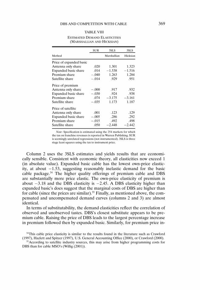
With the estimates of all of the model parameters, we can compute the ownand cross-price elasticities for each television choice. In column 1 of Table VIIIwe present results using the SUR estimates from the fixed effects regression.Assuming no endogeneity problems leads to estimates of the own price elas-ticities of expanded basic, premium, and satellite that are slightly positive,implying that television demand is almost completely insensitive to price.33

33For a discussion of the importance of instruments in the context of estimating welfare gains,see the debate in Hausman (1997b), Hausman (1997a), Bresnahan (1997), and Petrin (2002).


TABLE VIII

ESTIMATED DEMAND ELASTICITIES(MARSHALLIAN AND HICKSIAN)

SUR 3SLS 3SLS

Method Marshallian Hicksian

Price of expanded basicAntenna only share 020 1301 1323Expanded basic share 014 −1538 −1516Premium share −040 1263 1284Satellite share −014 929 951

Price of premiumAntenna only share −000 917 932Expanded basic share −030 924 938Premium share 074 −3175 −3161Satellite share −035 1173 1187

Price of satelliteAntenna only share 001 123 129Expanded basic share −005 286 292Premium share −015 492 498Satellite share 050 −2448 −2442

Note: Specification is estimated using the 254 markets for whichthe tax on franchise revenues is reported in Warren Publishing. SURis seemingly unrelated regressions (not instrumented). 3SLS is threestage least squares using the tax to instrument price.

Column 2 uses the 3SLS estimates and yields results that are economi-cally sensible. Consistent with economic theory, all elasticities now exceed 1(in absolute value). Expanded basic cable has the lowest own-price elastic-ity, at about −153, suggesting reasonably inelastic demand for the basiccable package.34 The higher quality offerings of premium cable and DBSare substantially more price elastic. The own-price elasticity of premium isabout −318 and the DBS elasticity is −245. A DBS elasticity higher thanexpanded basic’s does suggest that the marginal costs of DBS are higher thanfor cable (since the prices are similar).35 Finally, as mentioned above, the com-pensated and uncompensated demand curves (columns 2 and 3) are almostidentical.

In terms of substitutability, the demand elasticities reflect the correlation ofobserved and unobserved tastes. DBS’s closest substitute appears to be pre-mium cable. Raising the price of DBS leads to the largest percentage increasein premium followed then by expanded basic. Similarly, for premium price in-

34This cable price elasticity is similar to the results found in the literature such as Crawford(1997), Hazlett and Spitzer (1997), U.S. General Accounting Office (2000), or Crawford (2000).

35According to satellite industry sources, this may arise from higher programming costs forDBS than for cable MSO’s (Willig (2001)).


creases, DBS has the largest cross-price, followed again by expanded basic.Consistent with the differences in observed characteristics, local antenna is nota close substitute to DBS.

7. CABLE’S RESPONSE TO DBS ENTRY

The incumbent firm’s response to entry is often an important part of theproduct-market competition. In most empirical work this effect is ignored,even though it can substantially impact consumer welfare. In the cases whereit is recognized (such as Petrin (2002) and Hausman and Leonard (2002)),incumbents are assumed to respond only by changing prices. Because of therapid rise of DBS and the fact that it is a higher quality alternative on manydimensions, we examine the response of both cable prices and cable charac-teristics to entry. To do so we use our 2001 cross-section of cable systems. Asa complement to these results, we also match the 2001 cable systems to theirprices and characteristics in 1994 to ask the same questions.36

The only previous analyses of the impact of satellite competition on cableprices come from two government reports: U.S. General Accounting Office(2000) and FCC (2002b). These studies use cross-sectional data and regresscable prices on satellite share, controlling for product characteristics anddemographic averages. These studies have found that increasing satellite pen-etration is associated with higher cable prices. Our data set (which comes froma different source) yields a similar finding in such regressions. However, sincesatellite share is neither exogenous nor likely to enter the equilibrium pricingfunction linearly, it is problematic to conclude that the positive correlation ofprices is, in fact, causal. For example, the positive correlation may simply re-flect the fact that within markets unobserved tastes for multichannel video arecorrelated.37

These difficulties are symptomatic of the fact that supply responses are hardto estimate. This is especially true when a more structural approach is de-sired. In addition to the demand side estimation, a structural approach requirescost measures for each product. It also requires the type of competition to becompletely specified (e.g. Cournot or Bertrand–Nash, static or dynamic).38

We—like most researchers—neither observe marginal costs nor know exactlywhat the mode of conduct is for the supply side. Given these difficulties, weintroduce a reduced-form approach that exploits our demand side estimates toconstruct an estimator for the value to consumers of the entry-induced changesin cable price and characteristics.

36This information comes from the 1995 Television and Cable Factbook.37Some of the previous work has tried instrumenting for the satellite share. Unfortunately, this

does not correct the inconsistency problem if the pricing equation is a nonlinear function of theDBS share (or exogenous instruments for satellite entry are not available).

38Often, the assumption regarding the type of competition is combined with estimates of de-mand side elasticities to infer markups and (thus) marginal costs.


Our approach is to estimate an equilibrium pricing function directly andthen use it to ask whether cable prices vary systematically with the qualityof satellite, holding the other market-level factors entering the equation con-stant. The demand side model coupled with micro/econometric theory impliesthat the price for cable is potentially a nonlinear function of all exogenous fac-tors that affect demand and supply. These include demographics, the observedcharacteristics of all the products in the market (including the identity of thesellers), the franchise fee, and proxies for the unobserved factors of each prod-uct (which, for cable, Table VII shows are strongly correlated with prices).39

To provide a measure of these unobserved factors, we turn to the estimatesfrom our demand model. They provide us with consistent estimates of themagnitude of unobserved characteristics and tastes (together) in the units ofutility for every product-market pair. These estimates are given by the residualsin (5), and are computed as a function of the estimated δ’s, β’s, and observedcharacteristics:

ξmj = δmj −βxmj − α0pmj(11)

Estimates for δmj, βxmj, and α0pmj for expanded basic and premium cable areavailable directly from the second stage regressions in Table VII. For satellite,programming characteristics and prices do not vary across U.S. markets, so anequivalent decomposition yields a residual that only differs from δmSat by aconstant; we just use δmSat as the satellite regressor (and provide a robustnesscheck below).

Our basic cable pricing equation is given in column 1 of Table IX. It treatscable prices as a linear function of many market-specific factors: the mean de-mographics, the observed characteristics of both expanded basic and premiumcable, including indicator variables for those systems belonging to the largestseven multiple system operators and indicators for the number of leading pre-mium channels equal to two, three, four, or five (six is the excluded group), thecity franchise fee, residuals for expanded basic and premium cable from (11)and, similarly, the satellite fixed effect δmSat.

Many variables enter significantly and with the anticipated sign, includingpay-per-view, over-the-air channels, and some of the premium and MSO own-ership indicators. In particular, entering most significantly are δmSat and bothof the cable residuals.40 Overall, the R2 of .62 suggests these factors havereasonable explanatory power for the cable price. We estimate several spec-ifications that included higher-order terms to check for the importance ofnonlinearities, testing for the significance of the sets of additional coefficients.

39We present only the regressions using the prices of expanded basic for simplicity but theresults for premium were very similar in every case.

40The standard errors for this and future regressions are all corrected for the fact that manyregressors are estimated (following Murphy and Topel (1985)).


TABLE IX

SUPPLY SIDE RESPONSE OF CABLE SYSTEMS

Price Price Price βxmBase βxmBaseExplanatory Variable Exp Basic Exp Basic Exp Basic (Chars Ind) ( Chars Ind)

δ∗mSat −2390 −2447 −2215 043 056

(552) (527) (804) (021) (022)δ∗mBase 5038 4083

(817) (1255)δ∗mPrem 3990 3980

(709) (1096)ξmBase 5175

(896)ξmPrem 3761

(755)Channel capacity 019

(012)Pay per view 3340

(692)Year fran began −004

(033)Over-the-air channels −122

(066)City fee (tax) 244 441 038 −004 −013

(243) (226) (357) (010) (065)βxmBase (for 1994) −8861

(3377)HH size 868 1588 4156 −037 −135

(1415) (1419) (2198) (060) (065)Male single 2746 5173 11994 −737 −624

(6287) (6134) (9575) (262) (282)Female single 4308 4096 1715 −353 −550

(4625) (4610) (7006) (193) (205)Rent 2062 525 −5365 371 400

(4943) (4857) (7700) (207) (229)Single unit −1377 −2121 −9855 −281 −095

(4434) (4430) (6762) (187) (201)Income −813 −887 −1201 −031 −013($10,000) (369) (348) (519) (015) (016)Education 2816 2955 1993 051 006

(1059) (1051) (1559) (044) (046)

94/01 Owner Ind No/Yes No/No Yes/No No/Yes Yes/Yes94/01 Prem Ind No/Yes No/No Yes/No No/Yes No/NoR2 627 582 377 187 704Observations 250 250 243 250 247

Notes: The levels/differences regressions use 2001/1994–2001 data. The δ∗ , βxmBase , and ξ’s are demand sideestimates of observed and unobserved quality (described in text). Demographics are franchise area averages. “94/01Owner Ind” is Yes if separate indicators are included for the 1994 or 2001 multiple system operators (all regressionsinclude some kind of proxy for ownership variables), and similarly for the top six premium channel indicators with“94/01 Prem Ind.” Standard errors are corrected for the estimated nature of some regressors.


This included second-order approximations using all squared and interactionterms for all programming characteristics (136 total extra regressors), usingjust demographics (an additional 28 regressors), and using just δmSat and thecable residuals jointly (an additional 6 regressors). None of these specificationsrejected the null hypothesis that all additional higher order coefficients equalzero. Finally, the results do suggest that, holding other factors constant, wheresatellite quality is higher, prices for cable are lower.41

Our preferred approach to evaluating the magnitude of the price effectwould be to assume that eliminating satellite is equivalent to reducing δmSat

until demand is zero (by, for example, raising satellite’s price to its reservationlevel). In our data, the lowest satellite share we observe is 2%, so instead we usethe pricing function to ask how cable prices would change if we reduced satel-lite quality in every market to the estimated δmSat from this market, holdingall other observed and unobserved characteristics and tastes for the productsconstant.42 The price regression suggests that doing so would raise the aver-age cable price by $4.17 per month, an increase of about 15%, holding otherfactors constant.

In general, the specification in column 1 can be very demanding on the data.Even with just four goods, a linear approximation has 25 regressors, and acomplete second-order approximation has 357 regressors (which exceeds thenumber of market level observations in our sample). A natural, more parsimo-nious alternative, and one that is perhaps easier to interpret, is to include justthe price-adjusted quality index given by

δ∗mj = βxmj + ξmj(12)

which adjusts each δmj by the price effect α0pmj (see (5)). For each good j,including the δ∗

mj index in place of each of the xmj and the ξmj as regressorsin the pricing function imposes kj restrictions, where kj is the number of ob-served characteristics for good j.43 This set of restrictions is equivalent to as-suming that the δ’s from the demand side are sufficient proxies for both the

41As an alternative specification, we also tried using OLS to decompose δmSat into a compo-nent related to geographic factors that may affect satellite reception such as the dish angle inthe franchise area (computed using the DirecTV Dishpointer, DirecTV (2000) for the primaryzip code in the DMA), the average elevation in the market, and the variance in elevation inthe market (computed for us by David Rowley of the Geophysical Sciences department at theUniversity of Chicago using the one degree U.S. Geologic Survey Digital Elevation Model for a30 pixel by 30 pixel area centered at the geographic center of the DMA), and the climate mildnessand brightness score (as measured by the Places Rated Almanac by Savageau and Lotus (1997)).The R2 of .05 yields estimates of satellite residuals that differ little from the estimates of δmSat.Including both the predicted value and the residual separately in the column 1 regression (in-stead of δmSat) results in an insignificant parameter estimate on the predicted value and a verysignificant coefficient on the residual that is virtually identical to the coefficient on δmSat fromcolumn 1.

42This is Greenfield, Wisconsin near Milwaukee.43The kj + 1 coefficients on each of the βkxmjk and the ξmj are assumed to be identical.


demand and supply factors entering the equilibrium pricing function. Column2 reports this regression, imposing these restrictions for both expanded basicand premium cable. The R2 falls from .62 to .58, an insignificant amount forthe number of restrictions, so the more parsimonious approach is not rejected.The coefficient on δ∗

mSat is almost identical to column 1, leading to a similarpredicted price change.44

We also use our matched sample of 1994–2001 cable systems to ask whethersystems appear to have changed their prices and characteristics in responseto DBS entry (since DBS essentially did not exist in 1994). The added com-plication, however, is that the differences in prices over time are potentiallya nonlinear function of all exogenous factors from both 1994 and 2001. Sincethe Forrester data was not collected in 1994, we cannot estimate the demandsystem for that year. Instead, we assume that the tastes β for observed char-acteristics are constant over time and construct an equivalent 1994 βxmj indexfor expanded basic, up to controlling for MSO effects (the MSO’s in 1994 aredifferent from 2001). Because of the data limitations, we cannot correct foreither the unobserved factors for 1994 (derived from the δ’s) or the 1994 de-mographic averages.

Column 3 reports this estimated specification. The R2 for the price differ-ences is still reasonably high at .38.45 The coefficients on the δ∗ terms aresimilar to the cross-sectional regression and all enter significantly. In particu-lar, the coefficient on δmSat is −222 (vs. −239 in the cross-section), suggestinga relative price increase of about $3.86 per month for the average system with-out DBS entry.46 Thus, the matched sample and cross-sectional predictions arevery similar.

These estimated price changes hold cable characteristics constant. Althoughharder to measure than changing prices, cable systems may have respondedto DBS competition by innovating on characteristics like channel capacity andpay per view availability, especially given the seven year time frame. Indeed,some industry sources have argued that changing quality has been one of themost important ways that cable responded to DBS growth (see Watts (2003)).To investigate this question we ask whether, for the characteristics we observe,higher measured observed characteristics are positively correlated with higherDBS quality.

44We also consider a restriction which specified prices as a function of relative quality indices,which leads to δ∗

mSat − δ∗mBase and δ∗

mPrem − δ∗mBase replacing δ∗

mSat δ∗mBase, and δ∗

mPrem as regres-sors. The R2 falls from .62 to .32, which rejects this restriction.

45We again found that all of the specifications including higher-order terms and interactionterms to test for nonlinearities as described above lead to no rejections of the null hypothesis oflinearity.

46Note that this does not imply average prices were 12% lower in 2001 than they were in 1994,only that prices were 12% lower than they would have been without DBS entry. Indeed, averagecable prices rose by more than 25% over this time period, much of it (according to the cablefranchises) due to the rising costs of programming (see the discussion in FCC (2002b)).


We look at both the cross-sectional data from 2001 (column 4) and thematched sample (column 5). To construct the dependent variable, we againuse the weights from the utility function to construct a characteristics’ indexdefined as βxmBase. Since we are trying to explain the characteristics’ index(and the change in it), we only use as regressors the market demographics, thefranchise fee, and δ∗

mSat. The R2 is .19 and δ∗mSat has a positive and significant

coefficient. The average predicted change for this index if every satellite sys-tem were moved to its lowest observed quality level is between .075 and .1 inthe two specifications. If we use the estimate of the marginal utility of incomefrom Table VII to translate this into a “price-equivalent,” the regressions sug-gest that, moving to the characteristics prior to satellite results in a welfare lossequal to between $1.04 to $1.38 per month.47 We emphasize that this calcula-tion provides only a lower bound on the improvements in quality that systemsundertook, as this index does not include all characteristics (e.g., whether dig-ital cable is available), just the ones we observe.

8. THE CHANGE IN CONSUMER WELFARE

The results from Sections 6 and 7 suggest that the introduction of DBS hasimpacted the welfare of both DBS and cable subscribers.48 In this section weuse the demand and supply estimates to compute the overall changes to eachgroup, and the aggregate effect (weighting each household equally). Our baselevel of welfare is that achieved by households in 2001 with DBS available asan alternative. We ask how much income would have to change for a house-hold to achieve that same utility level in 2001 with DBS not available (i.e., thecompensating variation).49

We write compensating variation for household n as yn. Formally defined, itis the difference in the value of the expenditure function between the two eco-nomic environments under consideration. Let Vn = V (p0 yn n) be the welfarelevel in the base environment, that is, the highest utility household n with in-come yn can achieve when facing prices/characteristics p0 available in 2001 withDBS in the market. The expenditure necessary for household n to achieve Vn

is given by en(p0 Vn). Defining p1 as the prices/characteristics faced in thecounterfactual of no DBS entry, the expenditure necessary for household n to

47The price equivalent is calculated by solving for the price increase that exactly offsetsthe increase in utility from the improved characteristics, or the p such that (say) 075 −312p = 0, where .312 is the estimated marginal utility of income from Table VII. Since theoriginal demand specification is estimated using weekly prices, this p must then be multipliedby (52/12) to get the monthly price equivalent.

48Local antenna subscribers in 2001 experience no change in welfare; without DBS, local an-tenna remains free and the cable alternatives get worse.

49See Diamond and McFadden (1974) or Hicks (1946). Hause (1975) and Mishan (1977) alsoprovide helpful discussions.


achieve Vn is en(p1 Vn). Our measure of household level compensating varia-tion is then

yn = en(p1 Vn)− en(p0 Vn)= en(p1 Vn)− yn(13)

Welfare increases for satellite consumers for two reasons. First, at the ob-served 2001 prices and characteristics, DBS consumers’ willingness to pay forsatellite exceeds the price. Second, the results from Sections 6 and 7 suggestthat, without DBS, almost all of these satellite consumers would subscribe tocable at both a higher price and a lower quality than that observed in 2001.Similarly for cable consumers, surplus increases because they pay both lowerprices and get higher quality cable than they would have without DBS entry.

A standard empirical concern when calculating welfare gains from newgoods is that much of the estimated gain may come from extrapolating anestimated functional form to areas outside the region of the observed priceand quantity variation (i.e., that the true maximum willingness to pay is notobserved in the actual price variation). To determine how important this is inour case, we provide a lower bound estimate on welfare by raising the priceof satellite to the largest observed difference in the actual data (as opposed toraising the satellite price to infinity as with compensating variation). Similarly,as described in the previous section, for cable subscribers our lower bound es-timate reduces the quality of satellite only to the lowest observed level of δ∗

mSat

observed in our data.We begin by reiterating the importance of the controls for unobserved qual-

ity. Generally, when the price sensitivity is biased toward zero, welfare isbiased upward. Without the controls for unobserved quality our estimates (incolumn 1 of Table VII) are so biased that the demand curve is actually slightlyupward sloping, a case for which welfare estimation makes little economicsense.

If cable prices and characteristics are held constant at their observed 2001levels, the corrected (i.e., 3SLS) estimate for the welfare gain to DBS usersaverages about $127 per year, or $10.58 per month above what they pay for theservice. When satellite prices are raised to only the maximum observed pricedifference in the sample, the per capita average is about $100. This confirmsthat most of our estimated welfare gain for DBS subscribers (almost 80%)comes from a part of the demand curve that is not extrapolated. If we calcu-late welfare assuming annual cable prices would be $4 higher per month with-out DBS (from the supply regressions), the average welfare gain increases to$175 per year rather than $127. Finally, adding the characteristics’ effect yieldsa total gain of almost $190 per year, the average additional amount a DBSconsumer would willingly pay every year (over what they currently pay), oncedifferences in cable franchises induced by DBS entry are taken into account.

Although our sample is not representative of the entire country, if we ex-trapolate our results to all 16 million DBS adopters at the time of our sample


(rather than just to the urban customers), it would imply an aggregate welfaregain of between $2.5 billion and $3 billion for DBS subscribers.

For cable subscribers, our results suggest that cable prices are at least $4per month lower than they would have been. In the aggregate, given the 70million cable subscribers, the price effect yields a total welfare gain of about$3.3 billion for the consumers that stay with cable. The quality improvementsto cable characteristics are worth approximately another $1 per month of sur-plus, which adds another $800–900 million to the welfare change. In the end,while these supply-side calculations are less structural than the demand sideestimates, they point to a substantial aggregate welfare gain from DBS entryof as much as $4 billion per year for cable consumers.

9. CONCLUSION

Because DBS is the only direct competitor to cable in most markets, thenature of its competition with cable television is fundamentally important fordeveloping telecommunications policy. This paper examines the introductionof Direct Broadcast Satellites (DBS), the nature of that competition, and thewelfare gains satellites generate for consumers. We estimate a household-leveldiscrete choice demand system for satellite, basic cable, premium cable, and lo-cal antenna using micro data on the television choices of almost 30,000 house-holds, as well as price and characteristics data on cable companies throughoutthe nation. Our structural demand framework has extensive controls for un-observed product quality and permits the distribution of unobserved tastes tofollow a fully flexible multivariate normal distribution.

The results indicate that the own-price elasticity of expanded basic is atabout −15 while the demands for premium cable and DBS are substantiallymore elastic (−32 and −24). The cross-price elasticities suggest that DBS andpremium are the closest substitutes. The flexibility of the multivariate normaldistribution is crucial for understanding consumers’ true substitution patternsas the correlation of unobserved tastes for DBS and premium cable are partic-ularly high and are not captured in a conventional logit model.

Our approach to inferring the supply side response is more reduced form innature, using an estimated equilibrium pricing equation to ask whether cableprices vary systematically with the level of competition provided by satellite.The supply side results exploit the estimated controls from the structural de-mand side model and suggest that more competition from DBS is correlatedwith lower cable prices and somewhat higher quality cable. Overall there isa significant welfare gain to the 16 million satellite buyers between $2–3 bil-lion, depending upon whether changes in cable prices and characteristics areadded back into the calculation. The aggregate gains to the 70 million cableusers amount to between roughly $3–4 billion. In the end, our results suggestlarge gains from DBS entry, some of which are not captured if the price and


characteristics’ response is ignored. The overall gains from this product intro-duction may be as large as $7 billion, illustrating once again the importance ofunderstanding the impact of new goods on consumer welfare.

Graduate School of Business, University of Chicago, 1101 E. 58th St., Chicago,IL 60637, U.S.A.; [email protected]; http://gsbadg.uchicago.edu

andGraduate School of Business, University of Chicago, 1101 E. 58th St., Chicago,

IL 60637, U.S.A.; [email protected]; http://gsb.uchicago.edu/fac/amil.petrin.

Manuscript received March, 2002; final revision received August, 2003.

APPENDIX

If there is no sampling error in the product-market shares, the usual formulas for the stan-dard errors of the likelihood function estimates are valid for θ (with the fixed effect constraintsimposed). When sampling error enters the share estimates, it must be accounted for when com-puting the standard errors for θ (and δ).50 This appendix describes one method that accounts forthis source of error.

Before describing the method we follow, we begin at a more natural starting point for thinkingabout this correction, the first-order conditions of the likelihood function written with δ as afunction of θ, or

∂L(θk δ(θ))

∂θk

= 0 (k = 1 K)

These moment conditions include a term that accounts for the derivative of the likelihood func-tion with respect to θ (holding δ constant), the derivative of the likelihood function with respectto each δ, and the derivative of each δ with respect to each θ. Obtaining estimates of the stan-dard errors of θ and δ requires one to differentiate these first-order conditions, a nontrivial taskrequiring the evaluation of some computationally difficult terms.

Instead of following this approach, we make use of the fact that we can characterize the as-ymptotic behavior of the parameter estimates using a generalized method of moments (GMM)representation (similar, e.g., to Petrin (2002) or Berry, Levinsohn, and Pakes (1998)). This char-acterization provides a set of moments that have derivatives that are much easier to evaluatenumerically.

There are two different types of moments that are zeroed at the estimates (θ δ). First, thedifference between the observed and the fitted shares for each product-market pair is zeroed, or

smj(θ δ)− smj = 0 ∀ j ∀m(14)

where smj(θ δ) is the predicted market share for product j in market m and smj is the observedmarket share. J ∗ (M − 1) of these moments are independent (one moment in each market isredundant because the shares in each market sum to one). In each market m there are Nm ob-servations on each moment (where Nm is the number of households observed in market m).

50Our estimates for market shares are constructed using between thirty and several hundredobservations per market.


The second set of moments are derived from the likelihood function itself. At the maximum,the first-order conditions for the likelihood function are zeroed for each of the K parametersin θ, holding δ constant. Thus, an additional K moments are given by

∂L(θk δ)

∂θk

= 0 (k = 1 K)

There are N observations on each of these moments, where N = ∑Mm=1 Nm .

To compute the standard errors, all of the moments must be written in terms of the overall Nobservations. To do so, the first set of moments in (14) are reexpressed to yield the share ofadopters of good j in market m in the entire sample of N observations. For good j in market mthis moment is given by∑N

n=1 Im(n)Ij(n)

N

where Im(n) is an indicator that is on if individual n resides in market m, and Ij(n) is an indicatorthat is on if individual n purchases good j.51 The transformed moments—which are also zeroedby the parameter estimates—provide for a common index n = 1 N for all of the observa-tions entering the estimator, which is equivalent to multiplying each of the moments from (14)by Nm/N , a weight that accounts for the differences in market sizes.

Having transformed the moments so that each observation contributes to every moment, theasymptotic behavior of all parameter estimates can be represented as a function of N . If thestandard regularity conditions for GMM estimators hold in this data, the parameter estimates(θ δ) are asymptotically normally distributed around the true values (θ0 δ0) and can be writtenin terms of N , the variance of the (stacked) moments V evaluated at (θ0 δ0), and the matrix ofmoment gradients Γ with respect to θ and δ (also evaluated at (θ0 δ0)):

√N

(θ− θ0

δ− δ0

)A∼ N

(0 (Γ ′ Γ )−1 Γ ′ V Γ (Γ ′ Γ )−1

)

Because Γ is a square invertible matrix, we can rewrite this as

√N

(θ− θ0

δ− δ0

)A∼ N(0 Γ −1V Γ ′−1)

Reported standard errors evaluate Γ and V at (θ δ) using numerical approximations when nec-essary.

REFERENCES

ANDERSON, S. P., A. DE PALMA, AND J.-F. THISSE (1992): Discrete Choice Theory of Product Dif-ferentiation. Cambridge, MA: MIT Press.

BAJARI, P., AND L. BENKARD (2001): “Discrete Choice Models as Structural Models of Demand:Some Economic Implications of Common Approaches,” Working Paper.

BERNHOFF, J., S. MORRISETTE, AND K. CLEMMER (1998): “Technographics Service Explained,”Forrester Report, Vol. 1, Issue 0.

BERRY, S. T. (1994): “Estimating Discrete-Choice Models of Product Differentiation,” RANDJournal of Economics, 25, 242–262.

BERRY, S., J. LEVINSOHN, AND A. PAKES (1995): “Automobile Prices in Market Equilibrium,”Econometrica, 63, 841–890.

51Predicted market shares are computed in a similar manner using the model.


(1998): “Differentiated Products Demand Systems from a Combination of Micro andMacro Data: Autos Again,” Working Paper.

BERRY, S., AND A. PAKES (1999): “Estimating a Pure Hedonic Discrete Choice Model,” WorkingPaper, Yale University.

BRESNAHAN, T. (1997): “The Apple–Cinnamon Cheerios War: Valuing New Goods, Identify-ing Market Power, and Economic Measurement,” Draft Comment, http://www.stanford.edu/∼ tbres/research/replytobresnahan.pdf.

CHIPTY, T. (2001): “Vertical Integration, Market Foreclosure, and Consumer Welfare in the Ca-ble Television Industry,” American Economic Review, 91, 428–453.

CONSUMERS FEDERATION OF AMERICA (2001): “Lessons from 1996 Telecommunications Act:Deregulation Before Meaningful Competition Spells Consumer Disaster,” Unpublished Re-port, Consumers Federation of America.

CRAWFORD, G. S. (1997): “New Products, New Programs, and Prices: Measuring Con-sumer Benefits to Changes in Cable Television Choices, 1989–1995,” Working Paper,http://uaeller.arizona.edu/∼ crawford/research/cableind.html.

(2000): “The Impact of the 1992 Cable Act on Household Demand and Welfare,” RANDJournal of Economics, 31, 422–449.

DIAMOND, P., AND D. MCFADDEN (1974): “Some Issues of the Expenditure Function,” Journalof Public Economics, 3, 3–21.

DIRECTV (2000): “Dish Pointer, http://www.directv.com/howtoget, accessed January 15, 2000,”Discussion paper, DirecTV.

ELLICKSON, B. (1979): “Hedonic Theory and the Demand for Cable Television,” American Eco-nomic Review, 69, 183–189.

FCC (2001): “Federal Communications Commission Annual Assessment of the Status of Com-petition in the Market for the Delivery of Video Programming,” Seventh Annual Report, CS01-001, http://www.fcc.gov/mb/csrptpg.html.

(2002a): “Federal Communications Commission Annual Assessment of the Status ofCompetition in the Market for the Delivery of Video Programming,” MB Docket No 02-145,http://www.fcc.gov/mb/csrptpg.html.

(2002b): “Federal Communications Commission Statistical Report on Average Rates forBasic Service, Cable Programming Service, and Equipment,” MM Docket No 92-266, http://www.fcc.gov/mb/csrptpg.html.

GOOLSBEE, A. (2000): “In a World Without Borders: The Impact of Taxes on Internet Com-merce,” Quarterly Journal of Economics, 115, 561–576.

GREGORY, K., D. BRENNER, M. SCHOOLER, AND D. NICOLL (2000): “Reply Comments of theNational Cable Television Association in the Matter of Annual Assessment of the Status ofCompetition in Markets for the Delivery of Video Programming,” FCC CS Docket No 00-132,http://www.fcc.gov/mb/csrptpg.html.

HAUSE, J. C. (1975): “The Theory of Welfare Cost Measurement,” Journal of Political Economy,83, 1145–1182.

HAUSMAN, J. (1997a): “Reply to Professor Bresnahan,” Draft Comment, http://www.stanford.edu/∼ tbres/research/hausmanrecomment.pdf.

(1997b): “Valuation of New Goods Under Perfect and Imperfect Competition,” in TheEconomics of New Goods, ed. by R. Gordon and T. Bresnahan. Chicago: University of ChicagoPress, Chap. 5, pp. 209–237.

HAUSMAN, J., AND G. LEONARD (2002): “The Competitive Effects of a New Product Introduc-tion: A Case Study,” Journal of Industrial Economics, 50, 3, 237–263.

HAUSMAN, J., AND D. WISE (1978): “A Conditional Probit Model for Qualitative Choice: Dis-crete Decisions Recognizing Interdependence and Heterogeneous Preferences,” Economet-rica, 46, 403–426.

HAZLETT, T., AND M. SPITZER (1997): Public Policy Toward Cable Television. Cambridge, Massa-chusetts and Washington, DC: MIT Press and AEI Press.


HICKS, J. R. (1946): “The Generalized Theory of Consumers’ Surplus,” Review of Economic Stud-ies, 13, 68–74.

JAFFE, A., AND D. KANTER (1990): “Market Power of Local Cable Television Franchises: Evi-dence from the Effects of Deregulation,” RAND Journal of Economics, 21, 226–234.

KIMMELMAN, G. (1998): “Time to Put a Lid on Cable Rates,” http://www.consumersunion.org/telecom/telecom.htm, accessed 5/14/2001.

LANCASTER, K. (1971): Consumer Demand: A New Approach. New York: Columbia UniversityPress.

MAYO, J., AND Y. OTSUKA (1991): “Demand, Pricing, and Regulation: Evidence from the CableTV Industry,” RAND Journal of Economics, 22, 396–410.

MCFADDEN, D. (1973): “Conditional Logit Analysis of Qualitative Choice Behavior,” in Frontiersin Econometrics, Vol. 3, ed. by P. Zarembka. New York: Academic Press.

(1986): “Econometric Analysis of Qualitative Response Models,” in Handbook of Econo-metrics, Vol. 3, ed. by Z. Griliches and M. Intriligator. Amsterdam: North-Holland.

MISHAN, E. J. (1977): “The Plain Truth About Consumer Surplus,” Zeitschrift für Nation-alokonomie, 37, 1–24.

MURPHY, K., AND R. TOPEL (1985): “Estimation and Inference in Two-Step Econometric Mod-els,” Journal of Business and Economic Statistics, 3, 370–379.

NIELSEN MEDIA RESEARCH (2002): “Nielsen Media Research Local Universe Estimates (US),”http://www.nielsenmedia.com, accessed January 15, 2003.

OWEN, B. (1999): The Internet Challenge to Television. Cambridge, MA: Harvard University Press.PARK, R. (1971): “The Growth of Cable TV and Its Probable Impact on Over-The-Air Broadcast-

ing,” American Economic Review, 61, 69–73.PETRIN, A. (2002): “Quantifying the Benefits of New Products: The Case of the Minivan,” Journal

of Political Economy, 110, 705–729.PETRIN, A., AND K. TRAIN (2003): “Omitted Product Attributes in Discrete Choice Models,”

NBER Working Paper 9452.PRAGER, R. (1990): “Firm Behavior in Franchise Monopoly Markets,” RAND Journal of Eco-

nomics, 21, 211–225.RUBINOVITZ, R. (1993): “Market Power and Price Increases for Basic Cable Service since Dereg-

ulation,” RAND Journal of Economics, 24, 1–18.SAVAGEAU, D., AND G. LOTUS (1997): Places Rated Almanac. New York: Macmillan.TRAIN, K. (1986): Qualitative Choice Analysis. Cambridge, MA: MIT Press, Chap. 1, 2.U.S. GENERAL ACCOUNTING OFFICE (2000): “The Effect of Competition from Satellite

Providers on Cable Rates,” Report to Congressional Requesters, GAO/RCED-00-164. Washing-ton, DC: Govt. Printing Office.

WARREN PUBLISHING (2002): Warren Publishing Television and Cable Factbook. Washington, DC:Warren Publishing Inc.

WATTS, T. (2003): “Outside the Box: Can DBS Compete Against Cable?” Sky Report,http://www.skyreport.com/skyreport/apr2003/040203.shtmfour.

WILDMAN, S., AND J. DERTOUZOS (1990): “Competitive Effects of Broadcast Signals on Cable,Attachment to Comments of National Cable Television Association,” FCC MM 89-600 90-4.

WILLIG, R. (1976): “Consumer’s Surplus Without Apology,” American Economic Review, 66,589–597.

(2001): “Declaration of Robert Willig on Behalf of Echostar Communications Corpo-ration, General Motors Corporation and Hughes Electronics Corporation,” Attachment A toConsolidated Application for Authority to Transfer Control, Vol. I, FCC Filing.

ZUPAN, M. (1989): “The Efficacy of Franchise Bidding Schemes in the Case of Cable Television,”Journal of Law and Economics, 32, 401–456.

the consumer gains from direct broadcast satellites and the ...

Documents

Transcript of the consumer gains from direct broadcast satellites and the ...