modulation techniques for range measurements from satellites

ERC/R&D 66-1017

MODULATION TECHNIQUES FOR RANGE

MEASUREMENTS FROM SATELLITES

¢D9

CO

LU

fD --m mag a.a.

m

COQ- u.

U

e_ t-o o

Contract Number NAS 12-146

FINAL REPORT

JUNE 1967

National Aer0nautics and Space Administration

Electronics Research Center

N68- 1313 2 i,

(PAGES) .

._ {NASA CR OR TMX OR AD NUMBER)

(THRU)

/

(CATEGORY)

SPECIAL INFORMATION PRODUCTSDEPARTMENT

GENERAL @ ELECTRIC

SYRACUSE,NEW YORK

DEFENSE ELECTRONICSDIVISION

• q

ERC/R&D 66-1017

MODULATION TECHNIQUES FOR RANGE

MEASUREMENTS FROM SATELLITES

Contract Number NAS 12-146

FINAL REPORT

JUNE 1967

National Aeronautics and Space Administration

Electronics Research Center

SPECIAL INFORMATION PRODUCTSDEPARTMENT

GENERALQ ELECTRIC

SYRACUSE,NEWYORK

DEFENSEELECTRONICSDIVISION

Section

II

III

IV

V

TABLE OF CONTENTS

Title

GENERAL

A. INTRODUCTION

B. PURPOSE AND ORGANIZATION OF THE REPORT

C. CONCLUSIONS

D. RECOMMENDATIONS

OPERATIONAL PARAMETERS

A. EXPECTED TRAFFIC

B. FREQUENCY ALLOCATIONS

C. GROWTH CAPABILITY

D. ORBIT PARAMETERS

E. PROPAGATION TIME DELAY EFFECTS

SINGLE PULSE AMPLITUDE MODULATION

A. TECHNIQUE DESCRIPTION

B. PERFORMANCE ANALYSIS

C. IMPLEMENTATION CONSIDERATIONS

MULTIPLE PULSE TRAIN RANGING

A. INTRODUCTION

B. TECHNIQUE DESCRIPTION

C. PERFORMANCE ANALYSIS

1. Orbit and Stabilization Effects

2. Frequency Effects

3. Multiple Access Capability

4. Growth Capacity

5. Error Analysis

D. AN ILLUSTRATION OF SOME PARAMETERS OF A PULSE TRAIN

RANGING SYSTEM

SIDE TONE MODULATION

A. TECHNIQUE DESCRIPTIONS


C. HYBRID MODULATION IMPLEMENTATION

1. Ground-to-Satellite Link

2. Satellite-to-User Link

3. User-to-SateUite Link

4. Satellite-to-Ground Link

Page

I-I

I-i

I-3

I-4

I-6

II-1

If-1

II-3

II-3

II-8

II-9

III-I

III-1

III-1

III-7

IV-1

IV-I

IV-2

IV-11

IV- 11

IV-11

IV-12

IV-13

IV-15

IV-16

V-I

V-I

V-7

V-10

V-19

V-19

V-19

V-19

Section

APPENDIX A

APPENDIX B

APPENDIX C

APPENDIX D

APPENDIX E

TABLE OF CONTENTS (CONT.)

Title

A MULTIPLE ACCESS APPROACH

WAVEFORM DESCRIPTIONS AND PARAMETERS

FM PULSE COMPRESSION




FM-CW TRIANGULAR MODULATION



1. Power Budget

2. Doppler Effects

3. Multiple Access

4. Growth Capacity

5. Equipment Considerations

6. Propagation Effects

7. Interference Effects

8. Detailed Performance Analysis


PSEUDO RANDOM CODE TECHNIQUES

A. INTRODUCTION AND CODE GENERATION

B. CODE PROPERTIES

C. PSEUDO NOISE CODE ACQUISITION

D. PSEUDO NOISE RECEIVER IMPLEMENTATION

E. MEASUREMENT ACCURACIES

F. ACQUISITION TIME

G. SUMMARY

H. DETAILED ANALYSES

1. Frequency Band Occupancy and Information Transfer Rate

2. Signal-to-Noise Ratio and Frequency Band Occupancy for Various Modesof Transmission

3. Multiplexing Speech and Ranging Channels and Range Determination

4. Modulation by Binary Sequence for Ranging and Acquisition Time

5. Binary Sequences That are Generated by Boolean Function of Component

Sequences and their Correlation Functions

6. Pseudo-Random Sequences and Shift Register Sequence Generators

7. Determine the Periods of Component Sequences in the Boolean Sequence

and the Actual Improvement in Acquisition Time

8. Auto-Correlation Function Shape

A-1

B-1

C-1

C-1

C-4

C-7

D-1

D-1

D-2

D-2

D-4

D-6

D-6

D-7

D-7

D-7

D-7

D-17

E-I

E-I

E-3

E-5

E-6

E-7

E-8

E-12

E-12

E-12

E-16

E-20

E-22

E-25

E-31

E-34

E-35

ii

Section

APPENDIX F

APPENDIX G

APPENDIX H

APPENDIX J

RE FERE NCE S

TABLE OF CONTENTS (CONT.)

Title

SQUARE LAW DETECTION AND POST DETECTION FILTERING OF

ASYMMETRICAL SIGNALS

MATCHED FILTERS AND AMBIGUITY FUNCTIONS

A. UNIFORM PULSE TRAIN

B. STAGGERED REPETITION INTERVAL PULSE TRAINS

C. CODED-PULSE PULSE TRAINS

D. MULTIPLE CARRIER PULSE TRAINS

RELATIONSHIP BETWEEN SYSTEM PARAMETERS

LIST OF SYMBOLS

Page

F-I

G-I

G-7

G-10

G-f1

G-12

H-I

J-i

R-I

iii

Figure

I-1

II-1

II-2

II-3

II-4

II-5

II-6

II-7

II-8

II-9

II-10

II-11

II-12

III-1

III-2

IV-1

IV-2

IV-3

IV-4

IV-5

IV-6

IV-7

IV-8

V-I

V-2

V-3

V-4

V-5

V-6

V-7

V-8

V-9

V-10

LIST OF ILLUSTRATIONS

Title

Satellite Communication Geometry

Expected Traffic

Earth's Shadow Geometry

Geometrical Multiplication of Measurement Errors

Recording of GEOS I Satellite Signal

Plot of Integrated Phase Difference

Plot of Integrated Phase Difference-Pass 23

Plot of Integrated Phase Difference-Pass 28

Total Path Length Change Accumulated from 90 ° Elevation (GMT:05.00-11:00)

Total Path Length Change Accumulated from 90 ° Elevation (GMT:l1:00-17:00)

Total Path Length Change Accumulated from 90 ° Elevation (GMT.17:00-23:00)

Total Path Length Change Accumulated from 90 ° Elevation (GMT:23:00-05:00)

Synchronous Satellite Coverage and Accuracy (VHF Ranging System)

Satellite Transmitter Power Requirements

Equipment Block Diagrams

Envelope of Typical Pulse Train

Hlustration of Pulse Train Waveform Spare

Pulse Train Detector

Multiple Pulse System

User Equipment

Satellite Equipment

Maximum Doppler Frequency Shifts and Reciprocal Doppler Due to 5600 Miles

Orbit Satellite and 2100 Miles per Hour Aircraft

Probability of False Address

Ground Station Typical Receiver and Tone Extractor

FM Side Tone Transponder

Maximum Sweep Rate versus Noise Bandwidth with Proportional Plus

Integral Control Filter

Change (feet) in One-Way Range Resulting in One-Degree Phase Changeat Receiver

Tone Signal Processing

Hybrid Ranging System

Satellite to User Transmitter

User CSSB-AM Receiver

Test and Calibration Set

Hybrid Modulation System Address Timing

Page

I-2

II-2

II-6

II-10

II-20

II-21

II-22

II-23

II-24

II-24

II-25

II-25

II-26

III-3

III-8

IV-1

IV-3

IV-5

IV-6

IV-7

IV-8

IV-12

IV-14

V-2

V-3

V-4

V-8

V-9

V-12

V-14

V-15

V-16

V-18

iv

LIST OF ILLUSTRATIONS (CONT.)

Figure Title

A-1

C-1

C-2

C-3

D-1

D-2

D-3

D-4

D-5

D-6

D-7

D-8

D-9

D-10

D-11

D-12

D-13

D-14

E-1

E-2

E-3

E-4

E-5

E-6

E-7

E-8

E-9

E-10

E-11

E-12

E-13

E-14

E-15

E-16

E-17

F-1

F-2

F-3

Multiple Access Timing

Pulse Compression Radar

Dispersive Element

FM Pulse Compression Radar

Transmit-Receive Waveforms

"Small" Doppler Effect

"Large" Doppler Effect

Frequency Difference Variation with Range

Sweep Frequency

Frequency Difference

I fbJ avg.[fb[ avg.

r in Fractions of P

r in Fractions of P

Ambiguity Interval Shift

Relationship of Ambiguity Interval and Bandwidth

Equipment Block Diagram

Equipment Block Diagrams

Basic Shift Register Action

Truth Table and Logic Symbol for Half-Adder

Sequence Generator (Pseudo Noise)

Maximal and Non-Maximal Length Sequences

Autocorrelation Function

Pseudo Noise Receiver Implementation

Autocorrelation FunctionsmFiltered and Unifiltered Spectra

Double Correlator Control Function

Acquisition Accuracy

Impulse Responses Obtainable with Various Sinusoidal Rell-Offs

Cross Approximation of Sinusoidal Roll-Off Lowpass Filter Characteristic tothe Linear Phase Lowpass Filter Characteristic

Various Spectra

The Correlator of Two Binary Sequence Modulated Waveforms

Auto-Correlation Function of U

Cross-Correlation of U and Its Components

Block Diagram of Correlation Receiver

Shift Register Sequence Generator

Square Law Device

FunctionS (_)x

Function S (k - _)X

A-3

C-2

C-3

C-3

D-2

D-4

D-5

D-8

D-9

D-10

D-11

D-12

D-13

D-14

D-15

D-17

D-18

D-19

E-2

E-3

E-3

E-4

E-5

E-6

E-9

E-10

E-11

E-13

E-16

E-17

E-23

E-28

E-30

E-31

E-34

F-1

F-3

F-3

LISTOF ILLUSTRATIONS (CONT.)

Figure Title

F-4

F-5

F-6

F-7

F-8

F-9

F-10

F-11

F-12

F-13

G-1

G-2

G-3

G-4

G-5

G-6

G-7

G-8

H-1

H-2

Function S (_- k)X

Function I@)

Function S (_)

Function S (_)n

2 n 2 @)Function S n ,

FunctionAc2 IS n(_-_c ) + Sn (_ + _c)_

FunctionA, 2 [Sn(_ _) + Sn(_ + _)J

Power Spectrum at Low-Pass Filter Output

Ideal Bandpas s

Power SpectrummSpecial Case

Plot of Ambiguity Surface for Single Rectangular Pulse

Plog of Ambiguity Surface for Single Gaussian Pulse

Sketch of the Ambiguity Surface of a Swept Frequency Pulse

Envelope--Recurrent Pulse Train with Staggered Interpulse Spacing

(Average Value of AT n = 0)

Illustrations of the Ambiguity Surface of Uniform Pulse Trains

(From Reference 4)

I11ustrations of Ambiguity Surfaces for Staggered Repetition Interval Pulse

Trains (From Reference 4)

Sketches of Ambiguity Surface of Pulse Train Consisting of Uniformly Spaced,

Pseudo Randomly Frequency _ifted Pulses (From Reference 4)

Thumb Tack Ambiguity Surface

Waveform Space (Ds = 2, m - 3)

Time Dimension of Waveform Space

F-4

F-5

F-5

F-9

F-10

F-10

F-II

F-12

F-13

F-16

G-3

G-5

G-6

G-7

G-9

G-10

G--II

G-13

H-3

H-5

vi

Table

II-1

II-2

III-1

III-2

III-3

V-1

V-2

D-1

E-1

LIST OF TABLES

Title

Possible Allocations for Navigation Satellite Use

Typical Available Powers (Synchronous Satellites)

Power Budget

Bandwidth--Range Resolution

FrequencymPulse Energy

Power Budget

Doppler _ift

Power Budget

Logic of Direct Portion

Page

II-4

II-6

III-5

III-6

III-7

V-11

V-12

D-3

E-34

vii

SECTION I

GENERAL

A. INTRODUCTION

This report contains analyses and evaluations of modulation techniques for range measurements from

satellites. The material is presented as an aid in the selection of concepts and in the design of systems

using satellites for navigation and traffic control. Satellites are attractive for these applications because

they can serve as relays for line of sight transmission between fixed earth stations and distant ships and

aircraft.

Present-day ship and aircraft long-range communications use ionospheric reflection in the medium

and high frequency bands from 3000 kHz to 30 MHz. Propagation at these frequencies is dependent upon

solar activity and the transmissions are not reliable. Satellites have already demonstrated that they can be

used to provide superior communications for these craft.

Figure I-1 depicts the transmission links between an earth station, a satellite and a user craft. High

signal-to-noise ratios can be achieved between the earth station and the satellite at the information rates

necessary for navigation and traffic control because it is practical to use high transmitter power and high

gain antennas at the earth station.

The transmission links between the satellite and the user craft present more difficult problems to the

system designer. The limitations are set by the energy available in the satellite and by the small aperture

of a mobile user antenna. Solar cells are the only currently available practical energy source for satellites

that must have a long life in orbit. They are not efficient and the number that can be attached to a satellite

of practical size and weight is limited so that the prime power available is on the order of 1 kW.

Fortunately, the state-of-the-art in satellite stabilization has progressed so that it is possible to use

the radiated energy efficiently. As indicated by the dotted lines in Figure I-l, it is possible to direct the

satellite' s transmitted energy towards the earth so that very little is lost in space.

In spite of the advantage gained by using a directive antenna on the satellite, its radiated energy is

spread over a very large area, and therefore the power density seen by a receiving antenna is small. The

power captured for the receiver is a function of the antenna' s physical dimensions. The system designer is

faced with the conflicting requirements for large capture area; wide beamwidth; and for aircraft, aero-

dynamic acceptability. The selection of an operating frequency for a system is involved in this trade-off.

For a given capture area, the antenna directivity increases as the frequency increases. At frequencies

above VHF it becomes necessary to point the antenna in the direction of the satellite and this introduces

design problems, particularly for aircraft application.

I-1

//

////

//

\\\\\\\\\\\\

Figure I-1. Satellite Communication Geometry

The transmission link from the user craft to the satellite will usually have a higher signal-to-noise

ratio than the link from the satellite to the user, because the transmitter power aboard the user craft can

be higher than the satellite transmitter power.

Economic considerations have an important influence on satellite and user equipment designs. A

satellite mean time to failure of approximately 5 years is desirable. Reliability of user equipment is also

important. While preventative and repair maintenance can be performed, the revenue lost by taking an

I-2

aircraft or ship out of service for maintenance must be considered in the maintenance cost. The cost and

ease of retrofitting existing aircraft to make them serviceable in a traffic controlled environment must be

taken into account in the system design.

Although the communication links between the satellites and the ground terminals require careful

engineering, successful transmissions between earth stations and aircraft through the Syncom and ATS

satellites have demonstrated the practical advantages of satellites for communication with mobile terminals.

The results have matched predicted performance and together with data available from other satellite experi-

ments, they serve as the basis for confident predictions that satellites can be used advantageously for navi-

gation and positionfixing.

B. PURPOSE AND ORGANIZATION OF THE REPORT

This report is limited to a consideration of position fixing by range measurements from two or more

satellites. It is further restricted to measuring range by measuring the propagation time of a radio fre-

quency signal from the satellite to the user craft and return. Propagation time is measured by introducing

a time marker on the radio frequency signal and measuring the time required for the marker to travel from

the satellite to the user and back to the satellite. There are several ways in which the time marker can be

modulated onto the radio frequency signal. The accuracy of the range measurement does not depend upon

the choice of the modulation technique. In theory the energy required for the measurement is very nearly

the same for every modulation technique. In practice they differ widely in their means of implementation,

and have a greater influence on system design than any other major consideration.

The four transmission links up and down between the earth station and the satellite and down and up

between the satellite and the user craft have such different characteristics that the best choice of modulation

technique for one link may not always be the best choice for another. The equipment complexity necessary

to change from one form of modulation to another must be assessed against the equipment complexity with-

out the change in technique and also against the benefits of such a change.

Section II of the report deals with requirements, constraints and parameters common to all of the

modulation techniques. It serves as the basis for the analysis of each technique.

Section III presents the single pulse ranging technique that has been used for many years in simple

radars. It is included as a basis for comparing the various modulation techniques. As an aid in making the

comparisons, a power budget table and graph are included showing the satellite to user path transmitter

power required for range measurements over a wide range of frequencies and system parameter values.

Section IV is devoted to pulse train ranging. Pulse train ranging differs from single pulse ranging in

that a coded sequence of pulses is transmitted instead of the single pulse. Section IV presents side tone

modulation, including a side tone-single pulse hybrid implementation.

Several appendixes are included to provide additional detail. Appendix A describes a multiple access

approach for a large number of users; Appendices B, G and H present additional information beyond that

discussed in Section IV regarding the properties and applications of pulse trains.

I-3

A number of modulation techniques were studied in detail. Several of them proved to have serious

limitations for the application. The analyses made during the study and the resulting evaluations of these

techniques are also included as appendices as follows:

Appendix C--FM Pulse Compression

Appendix D--FM-CW Triangular Modulation

Appendix E--Pseudo-Random Code Techniques

Recognizing the voluminous studies that have been accomplished on Pseudo Random Codes, Appendix E

examines those aspects of the technique that are unique to this application. The interleaving of ranging

information and data and voice information is analyzed. Also a detailed analysis of various techniques to

improve the acquisition properties of pseudo random code is presented.

Appendix F develops the evaluation equations for the hybrid assymetrical spectrum presented in

Section V.

Appendix J presents a list of symbols employed in each section of the report.

C. CONCLUSIONS

Range measurement accuracy and the energy required for measurement are theoretically very nearly

the same for all of the modulation techniques studied. The techniques differ considerably in equipment

complexity and compatibility with existing communications equipment and procedures. They differ also in

acquisition time, ease of addressing large numbers of users, and the methods for resolving ambiguity. As

a result of these differences, the techniques vary widely in the efficiency of their use of radio frequency

energy. Specific conclusions about each of the modulation techniques are summarized below.

• Single Pulse Modulation

1. The concept is simple and performance is easily predicted.

2. User equipment is simple, but it is difficult to equip the satellite for transmitting the required

high peak power.

3. It is highly efficient in the use of radio frequency energy.

4. It is efficient in the use of the measurement time available because ambiguities do not have to

be resolved.

5. Some loss of efficiency results because address codes do not contribute to the measuring

process.

6. It is compatible with existing AM receivers.

7. It requires high peak power.

• Multiple Pulse or Pulse Train Modulation

1. Each pulse in a multiple pulse address code can contribute to the measurement accuracy.

2. The basic transmitting and receiving equipment are the same as for single pulse ranging;

however, additional pulse processing equipment is necessary.

3. It is highly efficient in the use of radio frequency energy, because the pulse train can contain

the range measurement information and the user' s address and can also provide the ambiguity

re solution.

I-4

4. Flexibility mcodingdesi_ allowsa widevariationof system_rameter values.5. Bycomparison_th asinglepulsesystem,peakpulsepowercanbereducedbya factor_-

tween_ andntimes, wheren is thenumberofthepulsesin_e pulsetrain.i

6. _ a stable phase control clock is used in _e pulse processing equipment, the return trans-

mission from a transponder can be delayed until after the entire train is received. A single

antenna may be used for receiving and transmi_iag by the use of an electronic coaxial switch,

ra_er t_n a _plexer. Reception and transmission may be on the same frequency.

• FM _lse Compression

1. This is prima_ly a coding scheme for single pulse ran_ng.

2. The technique permits a wide range of trade-offs m range resolution, measurement time,

band_dth and peak power.

3. _en band_dth is limited, there is a _rect ratio between _ak _wer and range resolution.

4. The characteristics of _e dispersive elements in _e transmitter and receiver must be closely

matched.

• FM-CW Trian_lar Modulation

1. Measurement time is long and the measurement must be made in several _screte steps.

2. Acquisition and address times are long,

3. Bandwid_, accuracy and ambi_ity interval are inter-related.

4. The techmque is inefficient in the use of radio frequency ener_ because of the long measure-

ment time. _ ad_tion, ambi_ity resolution r_uires the measurement to be made in several

steps.

• Multiple Side Tone Modulation

a. Transponded FM Side Tone

1. Acquisition t_e on the return link from the user is so long _at it can seriously reduce

multiple access capability.

2. S_cial pu_ose phase locked transponders are required.

3. It com_rison with other techniques, transmi_ed power can be low since the receiver

bandwidth can be reduced to a few Hertz by means of tracking filters. _is advantage is

achieved at the expense of long ac_isition times.

4. _ a phase lock receiver is not used, relatively high transmi_er power is necessary of _e

FM _reshold effect in the receiver.

b. Hybrid AM _de Tone

This hybrid tec_ique is descried m detail m _ction V. FM side _ne is used from the

ground to the satellite, AM side tone from _e satellite to the user, and a single pulse return

from _e user _rou_ the satellite to _e _ound terminal.

1. A conventional _ receiver may be employed by the user.

2. Sisal processing equipment is relatively simple.

3. _st detection filtering contribu_s to high efficiency in the use of satellite energy.

4. A store-and-forward tec_ique may be _plemented in the user equipment to simpli_ the

s_ring of the antenna for transmi_ing and receiving.

I-5

5. A large multiple access capacity can be achieved with the use of a block code multiple

access concept as described in Appendix A.

6. As with all "CW"types of modulation, initial system acquisition creates an energy penalty

unless the system is near time saturation.

• Pseudo-Random Codes

1. Implementation is relatively complex.

2. Acquisition times are long.

3. The technique is relatively insensitive to interference.

4. Multiple addressing of many users is comparatively simple.

5. Data, voice and digital communications may be multiplexed with range measurements.

Pulse modulation systems are efficient in their use of both energy and time. Peak power is compari-

tively high. However, there are a number of coding techniques that allow variation in pulse system param-

eter values. In general, the larger the number of pulses in the waveform, the greater is the freedom in the

selection of parameter values. The equipment is not complex; however, as the number of pulses increases

and the coding becomes more complex, the pulse processing equipment also becomes more complex.

Continuous wave systems usually require low power. They are not efficient in the use of energy or

time because the acquisition time becomes long. Efficiency increases as the interrogation rate increases

toward a 100 percent use of the channel. Implementation can be simple or complex, depending upon the

trade-off between acqusition time and power.

Combination or hybrid systems, in which different modulation techniques are used on each transmission

link, should be considered for the design of any system. If the processing equipment to change from one

form of modulation to another is simple, the special problems of each link may be solved independently.

Multiple access capability is severely limited by the acquisition time on the links from the user to the

satellite to the earth terminal. Since the range from the user to the satellite is not known, there is little

a priori knowledge available for reducing acquisition time on the return signal. As a consequence, techni-

ques that require short acquisition times are to be preferred if the user interrogation rate is high.

D. RECOMMENDATIONS

The study did not lead to a recommendation of one modulation technique that would be best for all appli-

cations. However, recommendations are made for two important applications. Multiple pulse train modula-

tion is recommended for a navigation and air traffic control system operating in the 118 to 135 MHz VHF

band. It is further recommended that a hybrid technique using side tone ranging on the links to the user and

pulses on the return link be considered for L-band implementation of a navigation/air traffic control system.

I-6

Multiple pulse train ranging was found to have the following advantages for the VHF implementation:

1. The equipment can be compatible with presently used VHF aircraft transmitters and receivers.

2. User equipment cost is low.

3. The equipment may be easily retrofitted to existing aircraft.

4. It is possible to use pulsed data and voice transmissions in the range measurement process so

that one channel and one set of equipment can be used for all functions.

While equipment costs may preclude fully coherent signal processing, satellite peak power can be

reduced to almost the same level needed for continuous wave ranging through the use of non-coherent pro-

cessing of the pulse train.

The choice of a modulation system for L-band operation (1540-1660 MHz) is not as clear cut as the

choice at VHF. The trade-off between antenna effective area and beamwidth requires either higher satellite

power or the ability to point the antenna toward the satellite. The current state-of-the-art will not permit a

large enough increase in satellite power for non-directional antennas on the aircraft. L-band operation will

require that operationally and aerodynamically acceptable antennas be developed for high performance air-

craft. The trade-off between peak power and efficient use of the energy available in the satellite must be

examined for L-band operation.

Communication equipment for L-band is not presently available, so that completely new designs will

be required for L-band operation. When the application is defined in detail, each transmission link must be

examined to ascertain the optimum use of equipment, power and spectrum. Studies directed towards an

L-band navigation/traffic control system implementation should include consideration of the hybrid system

described in Section V.

Frequencies lower than approximately 100 MHz are not useful because uncertainty in propagation delay

and ray path bending in the ionosphere introduce such excessive range errors. Frequencies above approxi-

mately 500 MHz require directional antennas on the user craft. Such antennas introduce operational and

aerodynamic design problems.

I-7

SECTION II

OPERATIONAL PARAMETERS

A. EXPECTED TRAFFIC

Aside from average satellite consumed power, the major effect of traffic density on a satellite naviga-

tion system occurs at that point when the simple "one-at-a-time w'approach to measurements is exceeded.

For a satellite in a 24-hour orbit, an average round trip propagation time of 0.52 second per measurement

exists (earth to satellite to earth and return). Thus, for a fix of position to be made (at least two range

measurements) a single user essentially ties up the system for 1.04 seconds; allowing approximately 3460

fixes per hour. This assumes that range measurements are completed sequentially. Thus, if the expected

traffic requires a fix rate in excess of 3460 fixes per hour, some form of multiple access to the system will

be necessary. With parallel channel operation utilizing two satellites, the fix rate without multiple access

rises to 6920 per hour.

Several studies have been conducted to prepare estimates of expected traffic for such a system. A

result of the "Study of Satellites for Navigation" (NASw-740) predicted traffic similar to that shown as curve

A in Figure II-1. Since that time, development has begun on the large or "jumbo t, jet aircraft and the super-

sonic transport (SST) aircraft. Certainly these aircraft are going to make a large modification in the air

traffic market.

A British Ministry of Aviation study, including the effects of the large Jets and SST' s, has shown an

expected peak of aircraft in the air in the late 1970is. Barring a presently unforeseen large increase in the

air traffic volume, an actual reduction in numbers of aircraft is anticipated after this due to the gradual

take-over of SST's. To relate this study tothe NASw 740 study, a fix rate for the SST aircraft of threetimes

that of a subsonic jet was assumed. This assumption was based mainly on an expected air traffic control

desire to know an aircraftVs position (regardless of type of aircraft) within a certain maximum uncertainty.

This assumption, along with the British Ministry of Aviation prediction, was the basis of the additional

curve (B) in Figure II-1 which incorporates the effect of the large jets and SSTVs o

It should be noted that these predicted traffic curves are for the North Atlantic which is used as a

model for this modulation study.

The significance of these traffic predictions to the modulation study is that they greatly exceed the

3460 or 6920 fix rate per hour that is the threshold of a multiple access requirement. Thus, either multiple

channels or time multiple access, or both, will be needed to fully meet the system needs.

II-1

120

With Large Jets and SST

8o

Total

_ , c

_ 40 _

B

1960 1970

Year

1980 1990

Figure II-1. Expected Traffic

II-2

Noting that the traffic model used for the NASw 740 study was based on 25 to 50 percent use by air traffic,

the curves of Figure II-1 are suspect if applied to the air traffic control case. Since tight traffic control is

already becoming necessary, a more likely curve for fix rate is curve C of Figure II-1. This curve is

based upon a 100-percent use by air traffic. There will be times when 100-percent use will not be neces-

sary; however, if weather is not going to seriously disrupt traffic flow, an air traffic control system must

be capable of 100 percent use. The curves shown in Figure II-1 thus represent a composite of air traffic

density predictions and navigation traffic ground rules. The importance of these curves lies not in their

complete accuracy but in that they serve to define the bounds of an engineering study. The data ultimately

can be grossly wrong in either direction and not alter the fact that a modulation technique that allows

multiple access measurements will be needed.

B. FREQUENCY ALLOCATIONS

At this time it is nearly impossible to predict exactly what allocation for a navigation satellite system

may be made in the radio frequency spectrum. Table I represents a survey of the current allocations indi-

cating the frequencies that have similar usage and could be considered for the system without a greater

perturbation in international allocations. Except for the VHF and low UHF bands, there is not a great

amount of equipment already in use with users. This does not say, however, that the current equipment

could not be used. It may well be possible to precede a present VHF receiver, for example, with a simple

solid state crystal controlled converter and use the current receiver for a microwave band. This conver-

sion to higher frequencies carries the penalty of decreased antenna capture area. As a result the power

requirements will generally rise with increasing frequency. Such simple conversions are, perhaps, not

available for user transmitters, though they could likely be used as driver RF sources for higher frequency

transmit equipment. Thus, in studying the area of modulation techniques, a specific frequency band does

not necessarily rule out the importance of compatibility with present equipment. In a like fashion, it is not

mandatory that a user receive and transmit on the sameband, eventhough that is what present VHF systems

equipment usually do. Conversely, it may be desirable in some cases to have transmission and reception

on the same frequency. In any event, Table II-1 indicates the likely frequency bands for a navigation

satellite system.

C. GROWTH CAPABILITY

The purpose of this section is to organize an approach to evaluating the future traffic handling capacity

of various modulation techniques. The use of many satellites can undoubtedly increase a given systemVs

capacity, especially on a world wide basis. The amount of increase, per satellite, would be heavily

dependent on the system implementation of the satellite, however, the actual modulation technique involved

would have very little or no impact on the affect of multiple satellites. As a result, this section of the

report will treat the capacity problem on a "per satellite" basis.

In general, there can be two limits to the traffic capacity of a satellite. One restriction on the system

would be due to power limitations in the satellite. Another restriction is the time-bandwidth restrictions of

the system.

H-3

o°,..i

o

0_;w

..Q

c_

.o

Z

_o

o

oo

Q)

0

u

z

.o

c_

I ._I.

I

3

c_

I

o

o_I,o

o

_o o'._'_o

._ o._

i

_ ss s

co co co co _o co c_ _ co

"r ,_ A

• ° .

_v

• ° .o

_ o

._ t--

v_

el

el

ooooooo

._ ._._

o

_oc_

II-4

0

v

1:1Q

I::I

0

rn

0

Z

0

0f..,q

0

I

Q_

i

!!-_°,

®

J_

' !i_ H

_. s _ _i "__. ,o_ ,_ _I _

i

_ o_

i

I"I-5

To assess the power limitations of the satellite requires a survey of the state-of-the-art in long life

satellite power sources. The results of such a survey have indicated that through the next decade, solar

cell power sources will most likely remain superior in cost over other systems. For solar cell power

sources, typical available powers are summarized in Table II-2.

Table II-2

Typical Available Powers (Synchronous Satellites)

Gravity Gradient andFlywheel Stabilization

Spin Stabilization

Satellite s/LaunchVehicle

1/Arias Agena

2/Atlas Agena

Syncom

Spinning GlobalComsat

Satellite

/wei_htl

950 Pounds

425 Pounds (each)

76 Pounds

250 Pounds

Average PowerAvailable

10 3 watts--4 years

4 x 10 2 watts--4 years

28 watts--1 year

40 watts

A secondary limitation on available power is the earth' s shadow interruptions of the input power.

These interruptions require the satellite to carry sufficient batteries to handle the system energy require-

ments during the shadowed time. The solar cell input power must be sufficiently above the system energy

requirements during the illuminated portions of the orbit to recharge the batteries.

For a worst case shadow, where the satellite's orbital plane is not inclined with respect to the earth-

sun axis, the shadow time can be evaluated as pictured in Figure II-2 o

._j/

Figure II-2° Earth's Shadow Geometry

The time a satellite spends in the earth's shadow is then:

ST(R e - h sinj_)

(2-1)

II-6

where:Reh

ge

= radius of the earth

-- satellite altitude (from center of the earth)

= gravitational constant of the earth

S T = (0.458 - 0.615 x 10 -6 h)¢_ minutes

for h in nautical miles.

(2-2)

Thus, for a geostationary satellite, the maximum eclipse time is 67.4 minutes, occurring once a day

near the equinoxes. The satellite is not eclipsed near mid-winter and mid-summer. A medium altitude

satellite (6-hour period) is eclipsed for 43 minutes, four times a day. These times, then, represent the

worst case for "power off" operation. The peak energy requirements during these dark periods will deter-

mine the battery storage requirements for the payload power.

An evaluation of the capacity limit, set by time and bandwidth, requires an extensive study of measure-

ment geometry, channel availability and time delays. If there is no time interleaving of interrogations, the

round trip radio propagation time sets a capacity limit for high altitude satellites. A capacity limit due to

propagation time may be defined as:

1C T =

Tp (2-3)

where Tp is the round trip propagation time o

In the instance of satelliteswhere this propagation time is long enough to be limiting,a possible way

to avoid the fullpenalty is to intermix several messages during the propagation time. The limitof this

mixing is:

TpM =

T M + TA + T D + T G

where

TM = message length (in time)

TA = acquisition times that may be necessary for signal reception

T D = data gathering time (may be greater than T M if message integration is necessary)

T G = time guard band between messages.

(2-4)

Actually it does not make sense to intermix fractional messages so this factor may be further defined

as some K -M where K is constrained to be an integer.

II-7

Another factor of importance is the efficiency of a technique for gathering data which may be defined

as:

T M + T A

= TM + TA + TD (2-5)

As a function of these various factors the limit (due to time) of a modulation technique is defined as:

C = K • C T • 77 ° (2-6)

Of course, for multiple channel operation this value would be multiplied accordingly. Since the factor C T

is independent of the modulation technique, a time figure of merit for the growth capacity of a modulation

technique can be defined as:

F T = K • 77 . (2-7)

A possible implementation of multiple access that takes advantage of interleaving of messages is described

in Appendix A.

Thus, the various modulation techniques can be compared (with respect to growth limit) on the basis

of two factors:

1. Power efficiency with respect to both average and shadow power availability

2. Time figure of merit.

D. ORBIT PARAMETERS

One of the major effects, aside from the great propagation distances involved, of the orbit used for

the satellite is the geometrical degradation of the range measurements. As pointed out in the analysis in

"Study of Satellites for Navigation" (NASw-740), a simple range measurement from one satellite fixes a

user somewhere along a circle on the earth's surface. Ranging from two satellites yields two such circles

which usually intersect in two areas. For this system, some other navigation means (dead reckoning, sun

or star fixes, etc.) is needed to resolve the intersection ambiguity.

The size of the intersection area is a variable dependent upon the range measurement error, satellite

position errors and user position with respect to the sub-satellite point (that point on the earth's surface

directly beneath the satellite)o Analyses were performed on NASw-740 that were based upon 100-foot errors

in range measurements and in satellite position. For the higher frequency bands considered, these assump-

tions were reasonable. However, when the lower frequencies are considered, the available bandwidth is

constrained and the propagation errors due to the ionosphere increase. These factors can force the assumed

100-foot ranging errors to increase greatlymperhaps to as high as 3500 to 4000 feet (as examined in the

propagation time delay effects section (II-E) of this report_o

II-8

Since error results may not simply scale accordingly to the change in range measurement accuracy,

a computer analysis (pages II-17 and II-18) has been run to determine the effects of the measurement geom-

etry and the range measurement errors on the user position errors. Figure II-3 is a graph which illustrates

the geometrical effects. For example, for a user 76 nautical miles (140.8 KM) from the sub-satellite point

of a geostationary satellite, a unit range measurement error would result in a 54 unit error in the calculated

user position. However, as the user position becomes far from the sub-satellite point, the geometrical

degradation becomes much less (reducing by an order of magnitude when the user is 550 nautical miles

(1019 KM) from the sub-satellite point). The graph of Figure II-3 does not assume any position errors in

the satellite.

To evaluate, more completely, the expected fix accuracies of the system, another computer program

(pages II-11 to II-18) was run. This program was set up for either two or three satellites, with complete

freedom as error values and positions of the users and satellites. Five locations were considered:

1. New York to London great circle midpoint

2. New York Coastal area

3. Mid-Atlantic near equator

4. Just south of Canary Island

5. Mid-North Atlantic

As a point of interest the data also shows the effects of altitude errors. As is to be expected, the maximum

errors occur near the equator as the user approaches the mid-point of the two satellites. Also this analysis

includes in the error figure, the calculated altitude errors. As such, the fix "on the ground"error would be

less than calculated. This analysis presents the data as the root-sum-square of the three errors of a

rectangular coordinate set centered at the center of the earth.

While this analysis does not include all error sources, nor does it systematically include all coverage

areas, it does indicate the relative fix accuracy available from the results indicate that a range measurement

error of +_1000 feet (304.8 meters) is sufficient to provide a fix accuracy of one nautical mile throughout a

usefully large coverage area.

E. PROPAGATION TIME DELAY EFFECTS

An experimental investigation of propagation effects is presently being conducted at the GE Radio

Optical Observatory near Schenectady, New York. This investigation employs signals from the GEOS I

Satellite which is in an orbit inclined 59 degrees to the equator with a perigee of 1115 KM and an apogee of

2275 KM. Passes over Schenectady include all azimuth and elevation angles at changing times of day.

Passes have a maximum period of approximately 20 minutes, so that an essentially stationary ionosphere

is scanned.

II-9

lOO

E

O

1

lOO

Satellite

1000

User Location-Great Circle Distance from Sub-Satellite Point-Nautical Miles

10,000

Figure II-3. Geometrical Multiplication of Measurement Errors

II-lO

ERR 9:19 SN TUE 12/2_/66

CALCULATION OF GEOMETRY EFFECTS ON MEASUREMENT ERRORS FOR

RANGING FROM A SATELLITE TO THE EARTH'S SURFACE

F6R A SATELLITE ALTITUDE (NAUTICAL MILES) OF ? 19327

RANGE (NM) DISTANCE (NM) ERROR RATIO

19328 76.4256 54.¢429

19337 241.751 12.11¢819347 342.¢_3 8.56423

19357 419.¢_7 6.9985

19367 483.99 6.¢666119377 541.299 5.4314719387 593.163 4.96316

19397 64¢.9_5 4.5996194_7 685.387 4.3_686

19417 727.2_8 4._6463

19427 766.8_3 3.85995

19437 8_4.5_2 3.684_5

19447 84_.559 3.53_78

19457 875.177 3.39571

19467 9_8.522 3.27551

19477 94_.728 3.16766

19487 971.91 3. ¢7¢2119497 1¢_2.16 2. 98157

195_7 1¢31.57 2.9_53

19517 1¢6¢. 19 2. 826_419527 1¢88.11 2.7573

19627 1337.21 2.27457

19727 1549.41 1.99¢3719827 1738.32 1.79897

19927 191_.92 1.65967

2_27 2¢71.34 1.553¢5

2_127 2222.26 1.46851

2_227 2365.56 1.3997

2_327 25_2.59 1.34259

2_427 2634.38 1.29446

2_527 2761.72 1.25342

2_627 2885.25 1.218_8

2_727 3¢95.49 1.18742

2¢827 3122.86 1.16¢67

2_927 3237.73 1.13723

21¢27 335¢.4 1.11662

21127 3461.14 1._9848

21227 357¢.17 1._8249

21327 3677.7 1._684121427 3783.91 1._56_421527 3888.96 1._4521

21627 3993. 1._3579

21727 4_96.16 1._2765

21827 4198.57 1.¢2¢69

21927 43_.34 1._148422_27 44_1.57 I._i_4

22127 45_2.38 i._622

22227 46¢2.85 1._334

22327 47_3._8 1._136

22427 48_3.15 i._26

22527 4993.16 1._2

II-ii

ERR 9:19 SN TUE 12/2fl/66

CALCULATION OF GEOMETRY EFFECTS ON MEASUREMENT ERRORS FOR

RANGING FROM A SATELLITE TO THE EARTH'S SURFACE

FOR A SATELLITE ALTITUDE (NAUTICAL MILES) OF ? 5595

_RANGE - _(_N_M_) ...... DI _8IRAN_CE _(__NI_IJ...... ERROR RATIO .......................

5596 65.2765 46.16_2

56fl5 2fl6.533 1fl.35195615 292.256 7.32613

5625 358.153 5.99141

5635 413.8_6 5.19768

5645 462.926 4.65712

5655 5fl7.412 4.25887

5665 548.395 3.94992

5675 586.6_9 3.7_138

5685 622.564 3.49589

5695 656,631 3.32236

57_5 689._92 3.17337

5715 72_.162 3.fl4367

5725 75fl.fl16 2.92943

5735 778.793 2.82788

5745 8fl6.6_8 2.73682

5755 833.558 2.6546

5765 859,725 2,5799

5775 885.178 2.51164

5785 9_9.976 2.44896

7795 934.173 2.39116

5895 115_.97 1.98694

5995 1336.98 1.751

6_95 15fl3.73 1.5935

6195 1657.12 1.47995

6295 18_.63 1.39386

6395 1936.51 1.32629

6495 2_66.32 1.27189

6595 2191.21 1.22726

6695 2312._3 1.19_12

6795 2429.43 1.15887

6895 2543.96 1.13237

6995 2656._3 1.1_975

7_95 2766._2 1,_9_38

7195 2874.2 1._7375

7295 298_,85 i._5948

7395 3_86.17 1._4726

7495 319¢.36 1.¢3683

7595 3293.59 1,_28_1

7695 3396._1 1._2_61

7795 3497.75 1._145

7895 3598.95 1._958

7995 3699.7 1._576

8_95 38_.13 1._295

8195 39_.33 1._1_9

8295 4_fl_.38 1._15

8395 41_.39 1._7

II-12

WHERE_ 13:49 $1 THU 02/23/6?

IF YOU WISH THE USER COVARIANCE MATRIX PRINTED TYPE- I3IF NOT TYPE O? O

HOW MANY SATELLITES ARE THERE IN THE SYSTEM? 3

WHAT IS LATITUDE [DEG], LONGITUDE [DEG] AND ALTITUDE [NM]OF EACH SATELLITE

? 0,40, 19327,0,20, 19327,15,20, 19327WHAT ARE THE SATELLITE POSITION ERRORS [FT]? 100,.100, I00, I00, I00, I00, 100, I00, lO0

WHAT IS USER'S LATITUDE [DEG],LONGITUDE [DE.G],AND ALTITUDEEFT]

.? 54_27,35E3WHAT ARE THE RANGE AND ALTITUDE MEASUREMENT ERRORS 'EFT]'? 1000' 1000, 1000, 500

RSS POSITION ERROR [NM] -583697 [ 1.08101 KM ]

DO YOU WISH ANOTHER USER POSITION? IF SO, TYPE I;

IF NOT, TYPE O? I

WHATIS USER,S LATITUDE [DEG],LONGITUDE {DEG],AND ALTITUDE[FT]? 40,75, lOE3

WHAT ARE THE RANGE AND ALTITUDE MEASUREMENT ERRORS [FT]? 1000, 1000, 1000, 500 "

RSS POSITION ERROR [NM] .537737 [ .995889 KM]

DO YOU WISH ANOTHER USER POSITION? IFSO, TYPE lJ

IF NOT, TYPE 0? 1

WHAT IS USER'S LATITUDE [DEG],LONGITUDE [DEG],AND ALTITUDE[FT]? 1,3,4,40E3 _WHAT ARE THE RANGE IAND ALTI'TUDE MEASUREMENT 'ERRORS {FT]

? 1000, 1000, 1000, 500

\

RSS POSITION" ERROR [NM] .935353 [ 1.73227 KM ]

DO, YOU WiSH ANOTHER USER .POSITION? IF SO, TYPE.IJ

I F NOT, TYPEiO? 1

II-13

WHAT IS USER'S LATITUDE [DEG],LONGITUDE [DEG],AND ALTITUDE[FT]

? 25,25,30E3WHAT ARE THE RANGE AND ALTITUDE MEASUREMENT ERRORS EFT]

? 1000, 1000, 1000. 500

RSS POSITION ERROR [NM] .662812 [ 1.22753 KM ]

DO YOU WISH ANOTHER USER POSITION? IF SO, TYPE 13

IF NOT, TYPE O? I

WHAT IS USER'S LATITUDE [DEG],LONGITUDE [DEG],AND ALT.ITUDE[FT]? 35,,45,30E3WHAT ARE THE RANGE AND ALTIT'UDE MEASUREMENT ERRORS EFT]

I000, I000, 1000,500

RSS POSITION ERROR [NM] .538588 [ .997465 KM ]

DO YOU V.!ISIIANOTHER USER POSITION? IF SO., TYPE 13IF NOT, TYPE O? I

WHAT I,S USER'S UATITUDE [DEG],LONGITUDE [DEG],AND ALTITUDE[FT]? 54, 27, 35E3

WHAT ARE THE RANGE AND ALTITUDE MEASUREMENT ERRORS EFT]

? I000, 1gO0, I000, 50

RSS POSITION ERROR [NM] .550575 r i.0!967 KM ]

DO YOU WISH ANOTHER USER .POSITION? IF SO, TYPE 13

IF NOT, TYPE O? I

WHAT IS USER'S LATITUDE [DEG],LONGITUDE [DEG],AND ALTITUDE[FT]

? 40, 75, fOE3

WHAT ARE THE RANGE AND ALTITUDE MEASUREMENT ERRORS [FT].? . I000, !000, I000,50

RSS POSITION ERROR (NM] .511849 [ .947945 KM ]


IF NOT, TYPE O? 1

II-14

WHAT_IS usER's LATITUDE [DEG]ILONGITUDE [DEG,]_,AND ALTITUDE[FT]? Is34, 40E3

WHAT ARE THE RANGE AND ALTITUDE MEASUREMENT ERRORS [FT]? I000, IO00, I000, 50

RS$ P'OSITION ERROR INN] -913301 c 1.69i43 KM 3

DO YOU WISH ANOTHER "USER POSITION? IF SO, TY,PE I;IF NOT, TYPE O? l

WHAT IS USER'S LATITUDE [DEG],LONGITUDE [DEG]JAND ALTITUDE[FT]? 25,25, 30E3

WHAT-ARE THE RANGE ;_D ALTITUDE MEASUREMENT ERRORS-[FT]

? I 000, I000, I000, 50

RSS POSITION ERROR [NM] .583271 [ I: 08022 KM ]

DO YOU WISH ANOTHER USER POSITION? IF SOt TYPE 13IF NOT. TYPE O? I

WHAT IS USER'S LATITUDE [DEG],LONGITUDE [DEG],AND ALTITUDE[FT]? '35, 45, 30E3

WHAT ARE THE RANGE AND ALTITUDE MEASUREMENT ERRORS [FT]? lO00, I000, I000, 50

RSS POSITION ERROR [NM]'.'493927 £ .914753 KM ]

DO YOU WISH ANOTHER USER .POSITION? IF'SO, TYPE l;.'

IF NOT, TYPE O? 0 '

//

TIME: 59 SECS.

If-15

WHERE* 14"04 St THU 02/23/67

IF YOU WISH THE USER COVARIANCE MATRIX PRINTED TYPE 11

IF NOT TYPE O? 0

HOW MANY SATELLITES ARE THERE IN THE SYSTEM? 2WHAT IS LATITUDE [DEG]s LONGITUDE [DEG] AND ALTITUDE [NM]

OF EACH SATELLITE

? 01 401.1932710J 201 I932"/WHAT ARE THE'SATELLITE POSITION' ERRORS [FT]

? I00JI00_10011001 1001 lO0

WHAT IS USER'S LATITUDE [DEG]_,LONGITUDE [DEG]J, AND A'LTITUDE[FT]

? 541 2"7* 35E3WHAT ARE TH_ RANGE AND ALTITUDE MEASUREMENT ERRORS [FT]

? I0001 I000, 500

RSS POSITION ERROR [NM] t659525 £ I. 22144 KM" ]

DO YOU WISH ANOTHER USER POSITION? IF SO, TYPE I;IF NOTJ TYPE O? l

WHAT IS USER'S LATITUDE [DEG]ILONGITUDE [DEG]IAND ALTITUDE[FT]

? 40., 75, fOE3

WHAT ARE THE RANGE AND ALTITUDE MEASUREMENT. ERRORS [FT]

? I000_ 1000., 500

RSS POSITION ERROR ENM] .855408 [ t.5{_422 KM ]

DO YOU WISH ANOTHER USER POSITION? IF SO_, TYPE I;

IF NOT, TYPE O? I

WHAT IS LISER'S LATITUDE [DEG]JLONGITUDE [DEG],AND' ALTITUDE[FT]

? 1.34.40E3

WHAT ARE THE RANGE AND ALTITUDE MEASUREMENT ERRORS [FT]

? I000, I000. 500

RSS POSITION ERROR [NM] 8,44126 [ 15.6332 KM ]

DO YOU WISH ANOTHER USER POSITION? IF SO_, TYPE I;

IF NOT* TYPE O? I

II-16

WHAT IS USER'S LATITUDE [DEG]-LONGITUDE [DEG],AND ALTITUDE[FT]? 25,25, 30E3 "

WHAT ARE THE RANGE AND ALTITUDE MEASUREMENT ERRORS [FT]? I000, !000, 500

RSS POSITION ERROR [NM] ,702258 [ 1.30058 KM ]

DO .YOU WISH ANOTHER USER POSITION? IF SO, TYPE IJIF NOT, TYPE 07. I.

WHAT IS USER'S LATITUDE [DEG],LONGITUDE [DEG],AND ALTITUDE[FT]? 35, 45,30E3

WHAT ARE THE RANGE AND ALTITUDE MEASUREMENT ERRORS [FT]?' I000, I000, 500

RSS POSITION ERROR [NM] .698266 [ 1.29319 KM ]

DO YOU WISH ANOTHER USER POSITION? IF SO, TYPE I;IF NOT, TYPE O? !

WHAT IS USER'S LATITUDE [DEG],LONG!TUDE [DEG],AND _ALTITUDE[FT]? 54, 27, 35E3

WHAT ARE THE RANGE AND ALTITUDE MEASUREMENT ERRORS [PT]? I000, 1000'50

RSS POSITION ERROR [NM] .635435 [ I',17683 KH ]


IF NOT, TYPE O? I

WHAT IS USER'S LATITUDE [DEG],LONGITUDE [DEG],AND ALTITUDE[FT]? 40,75, lOE3

WHAT. ARE THE RANGE' AND ALTITUDE MEASUREMENT ERRORS .[FT]

? ,1000, 1000, 50

RSS POSITION ERROR [NM] .828499 1'. 53438 KM ]

DO YOU WISH ANOTHER USER POSITION? IF SO, TYPE I;IF NOT. TYPE O? 1

II-17

WHAT IS USER'S LATITUDE [DEG]JLONGITUDE [DEG],AND ALTITUDEEFT]

? 1,34, 40E3WHAT ARE THE RANGE AND ALTITUDE MEASUREMENT ERRORS [FT]

? 1000, 1000, 50

RSS POSITION ERROR [NM] 6,2616,_ [ 11.5966 KM ]

DO YOU WISH ANOTHER !_ISE.R POSITION? IF SO,, TYPE 13•IF NOT, TYPE O? 1

WHAT IS USER'S LATITUDE [DEG],LONGITUDE [DEG]JAND ALTITUDEEFT]? _5, _5, 30E8_.'!HAT .a.r,ETHE PANGE AND ALTITUDE MEASUREMENT ERRORS [FT]

? 1000, 1000, 50

F_SS FO£ITION ERROR [NM] .643123 [ 1. 19 106 I_M ]


IF NOT, TYPE O? I

WHAT 1.'3 USER'S LATITUDE [DEG],LONGITUDE [DEG],AND ALTITUDE[FT]? 35, 45,30E3

t,!HA7 ARE THE RANGE AND ALTITUDE MEASUREMENT ERRORS [FT]

? 1000, I000, 50

RSS FOSITION ERROR [NM] .66156 [ 1.22521 KM ]


IF NOT, TYPE O? 0

TIME: __I £ECS.

II-18

The satellite transmits very stable, phase coherent signals at 162 and 324 MHz. These are received

on highly stable phase-locked receivers at the Observatory. A 30-foot steerable antenna is used to receive

the signals so that the data is not corrupted by noise. The voltage controlled oscillators of the two-phase

locked receivers are on the same frequency. If there were no ionosphere, these oscillators would have a

constant phase difference between them when locked to the coherent signals from the satellitewi.e., doppler

shift is cancelled by this process. At a point in the frequency multiplying chains ,where both are at 162 MHz,

the signals are applied to a phase comparator and thence to a paper chart recorder. The integral of the

phase difference is also recorded. One cycle of phase difference is recorded each time the path delay differ-

ence changes by the period of one cycle at 162 MHz (6.07 feet). A portion of a recording is shown in Fig-

ure II-4.

Plots of integrated phase difference for three passes are shown in Figures II-5, II-6, and II-7. The

first indicates that the ionosphere was uniform in its structure, the second indicates a very irregular struc-

ture, and the third shows an interesting phase reversal that was observed frequently but only within narrow

azimuth and elevation limits. The reason for the phase reversals have not yet been determined, but it has

been noted that they occur when the ray path is through or along the edge of the auroral zone.

The phase difference recordings provide a direct and precise measurement of the difference in path

length change at 162 and 324 MHz. Assuming that the effects are proportional to 1/f 2, a close estimate of

the path length change can be made at 162 and, similarly, at 118 to 136 MHz.

Data from 36 passes, taken at various times of data were plotted to determine the path length change

due to the ionosphere for each 5-degree change in elevation angle. The results are summarized in Figures

II-8 through II-11, which can be used to determine the mean and the ninety percentile values at any eleva-

tion angle.

The values in Figures 1"[-8 to II-11 are not to be taken as total range error due to the ionosphere,

however, as they do not include the error at the zenith. In addition to phase measurements, highly accu-

rate, high time-resolution measurements were made at both frequencies through the passes. It is believed

that these data can be used to determine the zenith angle error for each pass. But the data analysis has not

yet been completed to provide that result.

The zenith angle range error can be estimated as follows:

S

_ 40 x 106fARg _ I Ndh . (2- 8)

- O

The range of values for the integral is from 10 i2 to 1014, depending on diurnal, seasonal, and solar activity

changes. Conditions of the ionosphere are known at any time, so that the range uncertainty can be reduced

to much less than the 50-to-5000 feet total variation of AR at VHF.g

II-19

324 LOCK/LEVEL 162 LOCK/LEVEL I/4 j:r _ 182

S/22/ES Clg4SZ1965-09A . _ COMPAiq||ONNAX. EL. 45" AT lilJ KH:AZ 186- 46E

Figure II-4. Recording of GEOS I Satellite Signal

II-20

L9

¢q

72

144 j

/360

/

720

1080

Elevation: Azimuth in Degrees

oo o. oo oo oo o, °o °o °°

2,5

Pass: 2A

Date: 4-8-66

GMT: 01:16

10

15

2O

o_

_9

L9

1440

0 5 10 20 30

Time in Seconds from Beginning of Pass

25

Figure II-5. Plot of Integrated Phase Difference--Pass 2A

1]-21

72

144

360

h_

720

1080

1440

Elevation: Azimuth in Degrees

............ ., ..

Pass: 23

Date: 5-2-66

GMT: 18:46

5 10 20 30


2.5

-- 5

*$

@J

lO

15 N

2o

25

Figure II-6. Plot of Integrated Phase Difference--Pass 23

II-22

Elevation:

tf_ C_l O0v-q v-q _•. ., o.v=_ Cr_ O0

0

/ \144

_ Pass:Date:

}' X GMT:360

(D

_J

720

i

1080

oo

Azimuth in Degrees

1440

tt_ ao ,$

&" _ &"

\

5 10 20 30


28

5-3-6618:50 --

2.5

q3¢D

10_

e,

15

2O

25

Figure II-7. Plot of Integrated Phase Difference--Pass 28

II-23

20O0

_ 1000

_ 0

90 80 70 60 50 40 30 20 10 0

Elevation Angle in Degrees

Figure II-8. Total Path Length Change Accumulated from 90" Elevation (GMT:05:00-11:00)

A

• ,-4 ._

3000

2000

1000

I

I !

Percentile

I/, 0

90 80 70 60 50 40 30 20 10 0


Figure II-9. Total Path Length Change Accumulated from 90 ° Elevation (GMT:l1:00-17 :00)

II- 24

.$ ._ 3000

_'N

_ 2000

ooo

I

Percentile

1

i

9O

90 80 70 60 50 40 30 20 10 0


Figure II-10. Total Path Length Change Accumulated from 90 ° Elevation (GMT:17:00=23:00)

_._

2000

1000

J !

Percentile

_ _ -10

-100090 80 70 60 50 40 30 20 10 0


Figure II-11. Total Path Length Change Accumulated from 90 ° Elevation (GMT:23:00-05:00)

II-25

Totalrangeerror atVHF may be estimated by combining the propagation errors and those due to

noise jitter on the ranging signals. Since each contribution is independent of the others, they may be com-

bined as their root-mean-square to provide a one-sigma estimate of their total contribution. The total

range measurement error is used in the computation of fix accuracy by applying the geometrical dilution

factor for the region of interest.

Figure II-12 shows estimated position error contours determined theoretically. An independent

estimate using the observatory measurements yielded a 3-sigma error of 30, 200 feet for a region of the

Atlantic near the theoretical 6-nautical mile, 3-sigma contour line of Figure II-12. The estimate is based

on the parameters selected for the system described in Section IV.

221 I "1 1

_ Satellites ]

Underlined Numbers are Absolute Accuracy, 3(_

Others are Relative Accuracy, 3_

Figure II-12. Synchronous Satellite Coverage and Accuracy (VHF Ranging System)

II-26

SECTION III

SINGLE PULSE AMPLITUDE MODULATION


Single pulse amplitude modulation is the simplest concept for ranging. It is of interest as a possible

method for implementation, particularly at lower frequencies, and it is of further interest because it can

serve as a basis for comparing modulation methods. To aid this comparison, power budget calculations at

representative frequencies and bandwidths are included in this section.

A range measurement is accomplished by first addressing the individual user with a digital address

sent as a sequence of pulses. A single ranging pulse of short duration follows. The address and ranging

pulse are sent from the ground station to the satellite, which repeats the sequence pulse by pulse. After

the user's equipment recognizes its own address, it repeats the ranging pulse, which is again transponded

by the satellite. The ground station measures the time between the two repetitions of the ranging pulse by

the satellite, and thus determines the two-way propagation time between satellite and user plus the response

time of the user and satellite transponders. When the known transponder response times are subtracted

from measurement, it yields the range from the known position of the satellite to the user.

The pulses are transmitted by keying the transmitter "on" for the pulse duration. They are detected

using envelope detectors.


No special requirements are placed on the orbit design. Attitude stabilization of the satellite is not

required for the basic measurement since the satellite serves only as a relay for the pulsed signals. Alti-

tude stabilization is desirable, however, to permit the highest possible gain for the satellite antenna. Maxi-

mum antenna gain is especially important with this method because it requires the highest peak effective

radiated power of all the methods considered. In fact, one of the strongest reasons for considering methods

other than this one is this high peak power requirement.

Envelope detection of an amplitude modulated pulse requires that its peak signal be considerably

greater than the root mean square noise power in the bandwidth occupied by the pulse. Time can be resolved

to a fraction of the duration of the pulse if the signal-to-noise ratio is high. Woodward, gives the following

relationship of time resolution, bandwidth, and signal-to-noise ratio:

1 (3-i)6T =

/_(R)I

III-1

where:

R

5r

= effective bandwidth of pulse

= ratio of received signal energy in pulse to noise density

= standard deviation of _ (seconds).

This equation applies if the bandwidth of the receiver is matched to the bandwidth of the pulse, and if

R is large. System design constraints are most likely to set limits on range resolution and bandwidth. With

these constraints, the signal-to-noise ratio is determined from Equation 3-1 and a power budget drawn to

determine peak transmitter power. Equipment state-of-the-art sets the limit on peak power. The intended

use of the system and frequency allocation regulations determine range resolution, operating frequency, and

bandwidth.

Power budgets were calculated for several postulated implementations of the method and plotted on a

chart (Figure III-1) to show required transmitter power for the links between the satellite and user.

Figure III-1 relates peak power to user antenna beamwidth. Beamwidth is an important parameter in

a ranging system design because it determines the magnitude of the antenna pointing problem faced by the

user and also the user antenna aperture and, hence, antenna gain and physical size. Hemisphere coverage

is desirable because it eliminates the pointing problem. In general, a practical upper limit for antenna gain

in most mobile applications may be between 10 and 15 db; that is, between approximately 60- and 30-degree

beamwidths for practical antennas.

The ordinates of Figure IH-1 may be read directly in watts for single pulse ranging, where N is one.

The 1/_'N factor on the left hand ordinate scale gives a lower bound of the reduction in peak power for the

average of a number of single pulse measurements or for a pulse train. They may be further reduced if

pulse compression is used.

No method of ranging is more efficient than single pulse ranging in terms of the energy required for a

range measurement, neglectingthe energy required for address, if it is assumed that noise in the channel is

Gaussian and that only one user is interrogated at a time. In practice, single pulse ranging may be slightly

more efficient than other pulse methods because the equipment is simple. For example, a matched filter

for a single pulse is the intermediate frequency amplifier of the receiver adjusted for proper bandwidth.

The slightly greater efficiency that may be achieved using single pulse ranging is of minor significance.

The high peak power may be an overiding disadvantage in some cases. Furthermore, energy needed for

addressing users and furnishing communications is much larger than that required for the actual range

measurement itself,

Efficiency of single pulse measurement is emphasized to point out that other methods may reduce peak

power but they do not save energy over single pulse ranging. They trade between time, bandwidth, and peak

power. They may offer some other advantages as well. For example, pulse train ranging may accomplish

both the addressing and the range measurement in one pulse train. Other methods may also provide better

protection against impulse noise for a given energy per interrogation.

III-2

107

4 GHz, 1 MHz bandwidth

-- _ including propagation

/allowances.

N = Number of pulses

in train.

106 If pulse compression is used,

_- peak power may be reduced bycompression ratio. 100:1 is

feasible.

101

1600 MHz, 50 kHz bandwidth

including propagation

allowances.

500 MHz, 1 MHz bandwidth

including propagationallowances.

104

t 50 kHz bandwidthincluding propagation

103 allowances.

50 kHz bandwidth

no allowance for propagation

variables.

15 kHz bandwidth

conservative allowance for

propagation variables

(lees than 0.1 percent fade-out)

102

} 15 kHz bandwidth

no allowanee for propagation

variables.

10 100 180

User Antenna Beamwidth-Degreee

Figure III-1. Satellite Transmitter Power Requirements

III-3

Table HI-1 includes power budget calculations for several representative frequencies and bandwidths.

Values selected for the various parameters are reasonable values, but some are subject to wide variation

depending on equipment design and propagation conditions, particularly at lower frequencies. The 125 and

400 MHz cases plotted in Figure III-1 indicate the ranges of these values at the two frequencies.

Tropospheric and ionospheric attenuation and scintillation are small most of the time, so that the 6 db

value at 125 MHz is conservative, except for infrequent periods lasting from minutes to approximately an

hour, when short period fading fluctuations much greater than 6 db may take place.

Multipath fading occurs when the signal reflected from the earthVs surface arrives out of phase and

tends to cancel the direct signal from the satellite. Reflection coefficient varies with ground conductivity,

sea state and polarization. The ratio of the direct and reflected signals depends on the beamwidth and

pointing direction of the userWs antenna. As the user moves, he may pass through regions where the direct

and reflected signals alternately add in phase and cancel, so that the received signal level varies between

enhancement and degradation in comparison with the direct signal above. Under some circumstances multi-

path can cause complete cancellation. When a directional antenna is pointed upward toward a satellite,

multipath fading may be small. For this reason, in plotting Figure IH-1, itwas not considered important

for user antenna beamwidths smaller than approximately 90 ° . Although it can be important at any antenna

beamwidth if the antenna is pointed close to the horizon.

Satellite antenna peak to full coverage allowance is affected both by antenna beam shape and satellite

stabilization. The earth subtends 17.5 degrees at synchronous altitude. A 17 db antenna has a beamwidth

of 24 degrees between its half-power points. The power budget assumed a satellite stabilization of approxi-

mately +-3 degrees so that a user who sees the satellite on the horizon would suffer the 3 db loss, if the satel-

lite were at maximum tilt in the direction away from him.

Polarization loss is affected by Faraday rotation and antenna design. Faraday rotation can cause more

than a 90 ° change in the polarization of a plane polarized wave at 500 MHz, and much greater rotation at lower

frequencies. Signal reduction due to Faraday rotation may be avoided by using circularly polarized antennas

on both satellite and user craft. Circular polarization on the satellite and linear polarization on the user

craft can eliminate polarization fading, but cause a loss of 3 db in received signal. The power budget calcu-

lation assumed the use of circularly polarized antennas at both ends of the link. The -1 db allowance is for

ellipticity of the polarization.

Figure III-1 extends the power budget calculations to narrower antenna bandwidths. The calculations

and plots are presented without regard to whether they can be implemented. Peak power may be reduced at

least in proportion to square root of the number of pulses averaged, and in proportion to the pulse compres-

sion ratio, as explained in Appendix C. Hence, if 100 pulses were averaged, and each pulse were trans-

mitted with a 100:1 compression ratio, the peak power would be reduced by a factor approaching_/100 x 100 =

1000. Such reduction requires matched filter techniques, however. Simple envelope detection of pulses far

below the noise level is not possible. These considerations are discussed further in Section IV and

Appendix C.

III-4

ga

g_

A_I zttPI I

ZHPI 00g

g o]oH

• • . • o • • o o •

oo .oooo,o °

oo ..,,i., •

.o °,.°,oo o

oo ,o.oooo o

_m N

,_ o_.,_

_. _ ._

• ° • • • .....

• 0 ° o ° ° • o 0 •

• • ° ° • • . • o o

_-t I _1_-t i-4

• o o ° • •

+o o o + + I I + I

_J

° _ ._

_2, _ "_ WTwi:CI _) _)

•_ _, "_ OO

•,.._ o _ F_ = _.,..

_ _ g"_ _'_

oo

L-,,-

• . • o

.0oo

o

[" _ _ E",[-',

0

_. _._

_._ _

_ o

_ o

.,-i

,...i

_._ __._

o °

_.R_] _ _

_" o,_._ _._

'_o_oo_=

,-; d d

III-5

Envelope detection of the amplitude modulated pulses is not affected by doppler shift of the carrier

frequency.

The ultimate limit on interrogation rate is set by the differential propagation time to the various users.

Interrogations may be interleaved so that several can be made in the propagation time from the ground

station through satellite to user, and back. Various procedures for address coding and use of a priori knowl-

edge of user ranges may be used to program interrogations. This was discussed in Section II-C and an ex-

ample is presented in Appendix A.

Although single pulse ranging is well adapted to time division multiple access, it is not well adapted to

frequency division multiple access. The bandwidth of the range measuring pulses is wide compared to some

other ranging methods so that relatively small number of channels may be accommodated within a bandwidth

assignment.

Growth capacity is determined by the energy required for a range measurement and by multiple access

capability. The energy for the range measurement itself is small. The energy for addressing users and

transmitting their positions and other information is much greater than that for the measurement, and, thus,

is one of the limitations on total capacity. Multiple access capability is a limitation on growth capacity

because it determines the ability to use available channel assignments through multiplexing the transmissions.

Equation 3-1 relates bandwidth, signal-to-noise ratio, and resolution. If the noise in the channel is

Gaussian, white noise, the timing resolution can be a fraction of the pulse duration. For a 20 db signal-to-

noise ratio, thetiming resolution can be one-tenth the pulse duration. For the examples of Table III-1, a

20 db receiver output signal-to-noise ratio was assumed. Various bandwidths were used as examples. The

selections were made on the basis of fixed accuracy requirements as they are now understood for various

services.

The range resolutions of Table III-2 apply to each transmission link. There are a total of four links

in the measurement; ground station to satellite, thence to user, back to satellite, and from there to the ground

station. Because the ground station antenna can be large, thirty feet in diameter or larger, and the trans-

mission frequency and bandwidth can both be high on the links between the ground station and satellite, range

resolution can be sufficiently high that the links give a very small error contribution compared to the user-

satellite links. Range jitter on the links is not correlated and hence, the total error has a one sigma standard

deviation equal to the root sum square of the four link errors.

Table III-2

Bandwidth--Range Resolution

Pulse Prop. Time RangeService Bandwidth Duration Resolution Resolution

15 kHz 6.7 x 10 -6 sec.Air Traffic Control

Air and Marine

Position Fixing

High AccuracyMarine Position Fixing

50 kHz

1 mHz

0.67 x 10 -4 sec.

0.2x10 -4sec.

1.0 x 10-6 sec.

2.0 x 10-6 sec.

0.1 x 10-6 sec.

6700 feet

2000 feet

100 feet

III-6

Lapsedtimefor ameasurementof a user's range is essentially the propagation time from the ground

station to the satellite, thence to user and return; that is, approximately 0.5 second. Time for the signal to

pass through the satellite and user transponders must be added to the propagation time, but it is negligibly

small by comparison. For position fixing, measurements must be made from two satellites, but these may

be done essentially simultaneously so that both measurements are made in the same half-second. The results

of a previous study(2) indicated that the fix computation time was only about 3 ms in a large computer. Con-

sequently, the range measurements and fix computation can all be completed in a lapsed time of approximately

one-half second.

Equipment for single pulse ranging is conceptually simple. Important in the design of the user equip-

ment is the stability and uniformity of circuit delay between reception and retransmission of the pulses.

The delay must be constant and known to approximately one-tenth the duration of the pulse. It must be the

same for all user equipments. It is also critical to design the pulse detector for a consistent decision on

the timing of the pulse leading edge. Pulse shape must be maintained, and amplitude linearity must be main-

tained over a dynamic range sufficient to accommodate the full range of signal levels. An automatic gain

control must be provided to set and hold the gain from one received pulse to the next with a proper time con-

stant to accommodate changes in signal level. Fortunately, the dynamic range and gain control problems

are minimized because the total change in signal level due to the users' changing range from the satellite

is only about 1.5 db. While signal level changes due to atmospheric scintillation and multipath may be con-

siderably greater at lower RF frequencies, a dynamic range of 30 to 40 db should be sufficient for the re-

ceiver. Figure III-2 shows typical block diagrams for the ground equipment, satellite repeater and user

transponder.

Single pulse ranging is susceptible to impulse noise interference. Noise pulses that could be mistaken

for ranging pulses could cause a disruption of the system. Means to discriminate against noise pulses that

differ in amplitude or duration, or expected time of reception, can be provided to minimize the problem.

But the interfering pulses are similar to the ranging pulses and if they can occur within expected reception

periods, they could cause confusion in the measurements.


The energy in a pulse is its peak power multiplied by its duration in seconds.

lated in Table IH-1, the energies are:

For the examples calcu-

Table III-3

FrequencymPulse Energy

Peak Power Pulse Duration Energy

Frequency BW (watts) (seconds) (watt-seconds)

125 mHz

400 mHz

1600 mHz

4 gHz

500 mHz

15 kHz

50 kHz

50 kHz

1 mHz

1 mHz

1.00 x 103

2.5 x 103

6 x 104

7x106

4 x 104

67 x 10-6

20 x 10 -6

20 x 10 -_

10 -6

10-6

O. 067

0.05

1.2

7.0

0.04

IH-7

Address Code I

and Pulse

RangeGenerator

Iete ° Computer

ITransmitter

IPulse

Modulator

H Diplexer ___30-FootI _Antenna

I I IRangePulse

_ Gate _ Off

Counter ]

Receiver I_

Ground Station

Equipment

Diplexer H Receiver H G:

Address Code

Receiver and

I Communication

Transmitter

Satellite

Equipment

eHro erHoeer

[ G t L [ Rec ver

ViOiplexerH

Transmitter

ReceiverH Address Code

RegisterCommunicator

Gate

Display ]

Modulator

IUser

Equipment

Figure III-2. Equipment Block Diagrams

III-8

The energies shown in Table III-3 are selected as being within conservative design range for wide angle

antennas. They can be reduced in proportion to the curves of Figure IH-1 for user antennas of larger

aperture_i.e., narrower beamwidths.

Satellites of a cost and size considered to be economically attractive for the navigation functions can

supply bus power in excess of 150 watts. Assuming a transponder bus to RF efficiency of 33 percent,

50 watts is available for the navigation functions. The number of range measurements per second may be

determined by dividing energy in watt-second into the 50 watts available. For the values shown in Table III-3,

seven to several hundred range measurements could be made each second.

As noted above, the energy needed for addressing and transmitting fix information is much larger--in

the range of fifty to one hundred times the energy needed for the ranging above. Practical systems may,

therefore, be limited to the order of ten position fixes per second by the energy available in the satellite.

III-9

A. INTRODUCTION

In this technique,

Figure IV-1.

SECTK)N IV

MULTIPLE PULSE TRAIN RANGING

the ranging waveform transmitted is a group of pulses much as that indicated in

Amplitude

Time

Figure IV-1 o Envelope of Typical Pulse Train

Because the accuracy of a range measurement depends primarily upon the ranging waveform bandwidth

and the energy it contains, pulse trains have several desirable features. One is that the energy can be in-

creased by increasing the number of pulses without increasing the peak power. This is important because

many applications impose peak power limitations.

A second advantage exists when addressing or interrogating one of many users. In this case the pulse

train can be coded, for example, by coding the pulse spacing to make it serve as both the ranging waveform

and the address.

Figure IV-1 shows a simple pulse envelope _of pulses separated in time and implies a constant carrier

frequency. This is probably one of the most interesting cases. However, it should be noted that the pulse

train ranging technique need not be restricted to the use of such pulses. It is possible to utilize pulse to

pulse variation of carrier frequency and phase in addition to the staggering of the interpulse spacing as

indicated in Figure IV-lo Further, within the pulse envelope the frequency or the carrier phase can be

varied. These various forms of frequency and phase coding are particularly useful when it is necessary to

use minimum time for the rangingwaveform, when severe peakpower limitations exist, or when amplitude limit-

ing amplifiers are to be used in the system o Phase and frequency coding permit the time and bandwidth

allotted to the ranging waveform to be used most efficiently. When time duration is to be minimized, phase

or frequency ceding can be used to construct waveforms of nearly constant envelope amplitude. Hence the

energy is maximized; ye_ because of the coding, the bandwidth required for ranging accuracy and the possi-

bility of constructing various address codes is retained. Similarly, maximum bandwidth and energy can be

obtained when the peak power limitations are stringent. The use of amplitude limiting amplifiers require

phase or frequency coding to avoid signal suppression in the limiter. In general the detection of the pulse

train ranging waveform utilizes matched filters followed by detectors. The pulse train is most efficiently

detected through the use of a filter matched to the pulse train as a whole. However, considerations of

IVol

equipmentcomplexity,stabilityrequirementon oscillators and matched filters, the effects of Doppler fre-

quency shifts and repeater design may make the use of filters matched to the pulse train as a whole imprac-

tical. In this case, it is possible to detect the pulse train by parts,utilizing filters matched to the parts. In

the limit, the smallest parts of the pulse train are their individual pulses. When these are simple pulse

amplitude modulated carrier waveforms, the receiver IF amplifier can be a good approximation of a filter

matched to the individual pulses.

Individual pulse detection has the advantage that repeaters and transponders need only preserve the

envelope and phase relationship within a pulse; whereas detection of a pulse train by a filter matched to the

train as a whole requires that transponders and repeaters preserve the phase relationships between pulses

as well as the spacing of pulses. In the limit of simple amplitude modulated carrier pulses, individually

detected, the transponder can be a pulsed oscillator because phase coherence between pulses is not required.

The use of longcoherent processing times is limited by frequency stabilityrequirements, in additionto

equipment complexity. A serious loss of signal occurs for frequency shiftsequal to the reciprocal ofthe

processing time. However, this sensitivityto frequency shiftcan possibly be used to advantage in frequency

division multiplexing.

B. TECHNIQUE DESCRIPTION

This technique is based on the use of matched filters in detection of the pulse train. These filters,

discussed in Appendix G, coherently process the waveform to which they are matched. Generally, this gives

a time compression of the waveform, resulting in a pulsed waveform at the filter output which has a peak

signal-to-noise power ratio of about E/No; where E is the energy of the pulse train and No is the single sided

noise power density.

Appendix H introduces the concept of waveforrn space dimensionality and considers a method for

specifying waveforms in that space. Figure IV-2 shows diagrams illustrating waveform spaces of interest.

The largest space is that assigned to the complete pulse train and it has dimensions T s and Ws. As dis-

cussed in Appendix I_ in a space of this size waveforms with 2TsW s independent parameters may be speci-

fied. The independent parameters were taken as amplitudes of the waveform envelope spaced 1/2W s seconds

apart, in the case of low pass waveform s, and simultaneous samples of the inphase and quadrature compon-

ents of the waveforrn spaced 1/W s apart, in the case of bandpass waveforms. The smallest region of the

space to which a waveform can sensibly be confined has unit area in the passband case and considering the

inphase and quadrature components of the waveform, this allows 2TsW s elementary waveforms to be defined

in the space. This number is defined as the dimensionality of the space, D s.

It is convenient when considering pulse trains to divide T s into N intervals and define a pulse space

dimensionality Dp -- 2WsT, where T -- Ts/N. Each of the pulse waveforms with dimensionality Dw _ Dp isfitted into one of the pulse spaces. Figure IV-2 shows the pulse waveform made up from three short pulses

which may, for example, be phase shifted versions of each other. The resulting pulse waveform is shown

at various positions in the pulse space. Some of the many other possible ways of utilizing the space to define

pulse train waveforms are shown in Figure IV-2b, IV-2c, and IV-2d.

IV-2

ao

T-W

S

J__

1

•_w_ _-_ k I

S

bo

Lr

Co

T-W

S

J_T

TS

dl

T-W

S

J__

V/////A

"//////_

l_Tp V/////A

TS

Figure IV-2. Illustration of Pulse Train Waveform Space

IV-3

The method considered gives approximately orthogonal waveforms; the number being

M = D + 1P P

where

M = number of waveforms in pulse spaceP

D = dimensionality of pulse space = 2W T.p s

Which can be written as

(4-1)

M = 2TW + 1 . (4-2)p s

In order for a detector to distinguish between all these waveforms, it must have knowledge of the carrier

phase, in addition to the phase structure of the pulse waveform. In the system to be described, this informa-

tion is fairly easy to acquire on all links, except that, from user to satellite which would require an oscillator

synchronizing signal from the user. To avoid this complication and to give somewhat more conservative

results, the number of waveforms available is taken as

m = TW (4-3)S

_M for large TW2 p s"

As mentioned in the appendix, the waveforms, specified by the method described there, have optimally

low crosscorrelation coefficients, butnot necessarily good, uniformly low, crosscorrelation functions. It

is probable that a systematic transformation of the waveforms could be found, which would yield better

correlation functions. But since the transformation is not known, the number of available waveforms

specified is a reasonable approximation. References (3) and (8) give data useful in designing waveforms.

Figure IV-3 shows one way in which matched filters can be used in pulse train detection. It is appli-

cable only when the pulse waveforms have the same bandwidth and center frequency. It is not directly

applicable to the waveforms in Figure IV-2c and IV-2d. In Figure IV-3 the pulse train is applied to a par-

allel bank of matched filters. Each filter is matched to one of the N pulse waveforms. The response of

each matched filter is delayed to bring it into time coincidence with the other filter responses and detected.

The detected output may be applied either to a coincidence circuit or to a summing circuit and threshold

detector. A particular group of N pulses represents a user address. Coincidence of the N pulses or the

sum of the detected pulses exceeding a threshold notifies the user that he is being addressed.

R is apparent that the delay elements and matched filter can be interchanged assuming both are linear.

Alternately the detectors can precede the delays. When the pulse train is detected as a whole, only one

matched filter is used which incorporates the necessary delays and the detected pulse is applied to a thresh-

old circuit.

IV-4

PulseTrain

Input

IMatched Filters

No. 1

No. 2

Delays

No. 1

No. 2

No. N H No. N

EnvelopeDetector

H No. N _---_

CoincidenceDetector

or

SummingAmplifier

and

ThresholdDetector

Figure IV-3. Pulse Train Detector

The matched filter technique of Figure IV-3 can be used with equal bandwidth pulses in the train be-

cause each pulse has the same range resolving power as the train as a whole, although it contains less

energy. However, pulses of different center frequency such as shown in Figure IV-2c and IV-2d do not

individually have the bandwidth required for range resolution_the required bandwidth is contained in the

pulse train as a whole. Figure IV-3 can be adapted to such waveforms by removing the detectors and

summing the delayed responses before detection.

Detection of pulse trains as a whole has the primary advantage of minimizing both the peak and aver-

age power. The power is minimized because the pulse resulting from compressing the whole waveform

has the maximum possible amplitude, thereby giving least possibility for suppression by noise. If each of

the N pulses are individually detected, the energy is 1/N th of the train energy and greater suppression of

signal in the detector is possible. The advantages of long processing time are paid for by complexity in

the receiver in the form of the required matched filter and tighter tolerances on repeater performance.

Also, because pulse trains are comparatively long, the matched filter response is more sensitive to doppler

and other frequency shifts than is the response of a filter matched to the individual pulses. Appendix G

points out a serious loss of signal strength at the matched filter output for frequency shifts of about 1/t o,

where t o is the coherent processing time defined in Appendix B. to is not necessarily equal to the duration

of the signal as conventionally defined. The relationship can be found from the equations in the appendix.

However, it is convenient and in most cases adequately accurate, to take t o as equal to the conventional

duration of the waveform to which the filter is matched.

As illustrated in Appendix G, the sensitivity of pulse trains to frequency shifts can be utilized for

frequency division multiplexing. That is, with long pulse trains coherently processed by matched filters,

only small frequency offsets are required to greatly reduce filter response. Ambiguity functions of

Appendix G illustrate the effects.

IV-5

One possible implementation of the pulse train ranging technique is illustrated in Figures IV-4, IV-5, and

IV-6. The implementation is chosen to show general principles rather than to show an optimum configura-

tion. Figure IV-4 illustrates the operations to be performed by the system. Figures IV-5 and IV-6 provide

more detail on the user and satellite equipment. Pulse trains are used for both ranging and identifying the

user. The N different pulses making up the pulse train are taken as phase coded pulses chosen from a set

of k mutually orthogonal, equal energy, equal duration pulses, where N < k <- m. Each of the N pulses in

the train is detected through the use of a matched filter, followed by a square law detector. Pulse time

compression takes place in the matched filters and each of the N compressed pulses is detected and applied

to a digital matched filter which provides the delay and summing features described earlier.

User

Address

Detector

Address

Transmitter

Satellite

AddressEncoder

AddressDetector

k symbol alphabet

N symbols/address

Decoder

Encoder

Ground

Station

Figure IV-4. Multiple Pulse System

For illustration, the matched filters for the phase coded pulses are shown in Figure IV-5, as made up

from tapped delay lines. A single tapped delay line with N sets of tap weights, in a tap weight matrix, is

used to construct the N required matched filters. It is important to note that the pulse train detection is

done in two levels; first level is the pulse detection; the second level is the detection of a specific pulse

pattern.

An interrogation from a ground station via a satellite contains N pulses. The delay line, one set of

tap weights and a summing amplifier form a filter matched to a specific pulse waveform.

IV-6

I!

,a= o

I

Q) •

T

: I

z_ z_ z_

_e _e _ejY

xN_IAI 9,H_!OA_ d_&

:)

t_

t_!

IV-7

L

<

q

.1_ 0 ialO

I-_ I0 I

II

T-"

-'.i

I-- ----,

o_

in

!

0

IV-8

It is possible to have one or more of the pulse waveforms the same, except, for a time displacement

within the pulse space. In this case, onlyone set of tap weights is required for each pulse waveform.

The matched filter responses after detection are summed, used to phase control a clock and also

applied to a gate. Since the pulses making up the address are used in other user addresses, though not in

the same pattern, many pulses are used in controlling the phase of the clock. It is assumed that the ground

station interrogations are time quantized by a clock. The gate, driven by the synchronized clock, samples

the detected matched filter responses and applies them to the input of a shift register, which acts as a delay

line. N stages of the shift register are tapped to a summing amplifier. The taps correspond to the positions

of the detected pulses, which are sent to a threshold detector.

If some preselected level is exceeded at the threshold detector--meaning some preset number of

pulses in the train have been detected--a signal is generated to trigger a pulse code generator. The pulse

code generator forms an N pulse group corresponding to the time position of the pulses in the user pulse

train address. Each set of tap weights generates, in response to each pulse from the code generator, the

waveform to which the corresponding filter is matched. The pulse code enters the delay line at the opposite

end from the signal. Switches controlled by the pulse code generator select the time pattern of the phase

coded pulses for transmission. After summing the N pulses, theyare frequency translated and transmitted

to the satellite. IF, RF and power amplifiers, required in operational equipment, are not shown in the

figure. An important feature of this technique is the use of many received pulses to control clock phase.

This means the arrival time of an interrogation is known much better than could be determined from a

single pulse train. The function of the pulse train is to identify which of the clock pulses represents the

arrival time.

A variety of satellite equipment can be used with pulse train ranging. If the satellite-ground station

link is wideband and good quality, very little data processing is required at the satellite. For example,

pulse trains made up of phase or frequency coded pulses can be transmitted directly through amplitude limit-

ing amplifiers in the satellite. In this case, useraddress generation for interrogation and matched filter

detection of the user response can be done at the ground station with little loss in system performance.

When high energy pulse trains are used, itmay be more convenient to generate them in the satellite.

Figure IV-6 shows a possible implementation. The satellite equipment has separate receivers and trans-

mitters for communicating with the ground station and the user. It is assumed that power and receiver

sensitivity are not problems on the ground station to satellite link. Consequently, a modem different from

that on the user-satellite link might well be used to reduce the time required to send interrogations and

responses. Since this link is not critical, ithas not been analyzed. However, the ground station transmits

user addresses in some arbitrary format and the transmission contains timing information, so that trans-

missions to users can be accurately timed. The ground station transmission is detected and a pulse group

generated to excite the tapped delay line. Since the N pulses in the user pulse train address can be selected

from k possible waveforms, the tap weight matrix on the tapped delay line must contain k sets of weights.

Otherwise, the satellite equipment generates user addresses in the same manner as the user generates a

response.

IV-9

Receptionofuserresponsesalsorequiresk matchedfilters plusthedelayandaddfunction.Sincetheuseraddressis transmittedto thesatellitebythegroundstation,thisinformationis usedto simplifythereceivingequipment.

Detectedmatched filter outputs are fed to a decoder circuit which provides the delay and add function

through the use of a digital delay line. As the system has been described, no timing information is sent

from the user except that contained in the responded address. Because the arrival time of the user

response must be derived from the response, the detector output pulses must be sampled at a rate such

that several samples are taken of each pulse. This is necessary to achieve accurate definition of the pulse

leading and/or trailing edge. The shift register delay line clock must be at the sampling rate. Since the

total delay required is constant and equal to the address duration, the number of shift register stages re-

quired increases linearly with clock rate. This may make the technique unattractive when long address

duration are used.

One alternative to digital delay lines is the use of passive delay lines as the delay mechanism. A

passive delay line does not require sampling of the detector output. A second alternative is use of one of

the possible pulse trains exclusively for timing information. N detectors would be permanently wired to the

input of a passive delay line, tappedto detect the timing train pulse pattern. The address train arrival time

then would need only to be known accurately enough to gate the timing pulse to the encoders. The sampling

rate required for the other delay lines, if they are digital, is much lower than that needed to define the

beginning and end of pulses. Gating of the timing pulse is required only if user responses are allowed to

overlap in time at the satellite.

Since many user responses must be detected, it is cumbersome to have one delay line properly tapped

and connected to the detectors for each of the users. This is avoided through the use of the information

available at the satellite about the addresses currently in use. Specifically, each detector drives a bank of

parallel gates--the number of gates required at each detector is equal to the maximum number of addresses

that will be in use in any 43 microseconds interval. The 43 microseconds is the uncertainty in the user

response delay and is equal to the two way propagation time over the earth radius. One gate on each

detector is connected to a delay lin_ which is tapped at intervals equal to the minimum, discrete, position

the pulses can occupy in the pulse train. Each tap is gated to a summing amplifier.

For each address in use, the appropriate N detector gates are energized to pass the detected pulses to

a delay line. The delay line tap gates corresponding to the user pulse groups are also energized. Thus, a

detector for each of the addresses in use is set up. The detector remains set up for a maximum of

43 microseconds and then is readjusted to detect a new address.

The address information is delayed between the ground station decoder and the user response decoder

by a time interval equal to the fixed system delays, suchas the propagation time from satellite altitude to

the earth and back,

IV-10

C. PERFORMANCE ANALYSIS

1. ORBIT AND STABILIZATION EFFECTS

These factors uniquely affect this technique only through doppler frequency shifts produced.

effects are discussed below.

Doppler

2. FREQUENCY EFFECTS

The carrier frequency determines the space loss, antenna gain for a fixed aperture, scintillation due

to ionosphere and magnitude of doppler shifts. These effects are common to all techniques. Only doppler

has a unique effect on this system. So the discussion will be confinded to doppler.

The doppler frequency shift,one way, is given by

Z" __ f Hz (4-4)Vd c c

where

_t = range rate

c = propagation velocity

fc = the carrier frequency.

For a 5,600 mile orbit, the maximum range rate is about 4,200 miles per hour. A mach three aircraft can

contribute about 2100 miles per hour to the range rate. These range rates give maximum doppler shifts of

Vd, sat = 6.3'f cHz

Vd, ac = 3.15 fcHZ

for fc in megahertz. Over the frequency range of 118 to 1660 MHz, the maximum contributions to doppler

shifts go from Ud, sat = 744 to 10,460 Hz and Vd, ac = 372 to 5, 230 Hz. As discussed previously, the

detector output is low, if the waveform is mismatched by I/t ° Hz from the matched filter center frequency.

Consequently, uncompensated doppler limits the coherent processing time to

< i (4-5)to Vd, sat + Ud, ac

Automatic frequency control can be imcorporated into the system to compensate for doppler. Since

Vd, sat + Vd, ac can reach a maximum of 15, 690 Hz, the system would be limited to coherent processing of

simple pulses, if the system bandwidth is similarly restricted. Simple pulses require high peak power. The

peak power reduction possible is proportional to the dimensionality of the pulse waveform. Consequently,

if the bandwidth is restricted by assignment and doppler is large, high peak power is required.

Figure IV-7 shows maximum doppler shifts and the corresponding restrictions on processing time as

a function of carrier frequency.

IV-11

e_o

4 20

[ Vd, sat+ Vd, aJ

I/Vd, ac J3 I 15

/ 1/Vd, sat

i2

a 5"_ 1

00

Figure IV-7.

500 1000 1500 2000

Carrier Frequency--MHz

Maximum Doppler Frequency Shifts and Reciprocal Doppler Due to 5600 MilesOrbit Satellite and 2100 Miles per Hour Aircraft

3. MULTIPLE ACCESS CAPABILITY

The multiple access capabilities can be estimated as follows o Assume pulse train's made up of N

coded pulses. The coding is such that the pulses are nearly mutually orthogonal to eliminate considerations

of partial contributions. This may be achieved by a combination of time and phase coding. In any case, the

pulses are spaced by a nominal interval of T seconds. Each of the N places can contain one of k orthogonal

pulses. For example, if the pulses are simple, uncoded pulses may lie in one of k non-overlapping time

slots in the pulse space.

The limit of the multiple access capability technique is taken as the number of user response

pulse trains that may be simultaneously handled by the satellite receiver without the probability of falsely

generating an address currently in use exceeding some prescribed level. False addresses generated in

satellite transmission will with high probability be rejected by the satellite, if respondedto by a user. It is

assumed that each of the N pulses making up a train is chosen randomly from the set of k waveforms. The

random choice is for convenience in analysis and would not be used in practice, becauseofthe possibility of

duplicating addresses. However, such a choice results in a conservative estimate of the multiple access

capability.

IV-12

Let L be the number of user responses simultaneously arriving at the satellite. L is assumed to be

constant*. Let

Pl = probability that in the jth pulse period one of the L users has one of the k •

waveforms matching a given user address.

= 1/k

P2 = probability that none of the L users has the particular waveform in the interval

= (1-pl) L = (1- l/k) L

P3 = probability of one or more of the L users having the waveform in the given interval

-- - : -[1-(i- /z)Lj

P4 = probability of one or more of the L users having a given waveform in each of the N

intervals

= probability of falsely generating a given user address

: --[i- (i-i/k)L]N

If q is the number of addresses in use at a given time, the probability that one of them is falsely generated

is approximately

(4-6)

P5 = q P4 (4-7)

Figure IV-8 shows a plot of Equation (4-6) for N = 5, 10 and k = 5, 10, 20. It shows that the multiple

access capability is heavily influenced by the degree of security against false address generation required.

Note that the curves strictly apply only when the pulse waveforms are chosen randomly. Practically, the

would be chosen by design and this would decrease the probability of generating a false address, when L is

small, from that shown on the curves. For example, when L = 1, there is only one user transmitting to the

satellite and that waveform would be different by design from all other users. That would make the proba-

bility of false address zero. Therefore, the curves should go to infinity at L = 1. From a few calculations

wherein the non-random choice of waveforms is taken into account, it appears that the curves show a prob-

ability of false address that is large by a factor of 3--i.e., the curve are low by 1/2 division, at L = 2 and

the error is smaller for larger L.

In addition to the limitation on multiple access caused by false address generation, there is a limita-

tion due to interference between pulses. This is due to the fact that the k pulses cannot be strictly ortho-

gonal for all relative time displacements. This results in a low level noise-like response of a matched filter

to a waveform to which it is not matched. This point is discussed in Appendix G.

4. GROWTH CAPACITY

The example of paragraph D, which follows, shows that the technique is capable of handling more than

the expected traffic.

*L is actually not constant because the users are distributed in range. A more accurate result requiresaveraging over the distribution of L. See Reference (9).

IV-13

_z ._

'_ _ _

_._

/I'll

,ill_ i

II / ,i //i//, °: / ;

/ ///_I__ _I/d

I

,.-i ,-t ,...I ,.-4 I I I I I I I I II I I I I

(sso:tpp V ani_,4 lo £1t.l!qvqo,_d) Otto I

"0<

0

.,._

o.J

IV-14

5. ERROR ANALYSIS

The basic limitation on accuracy of the range measurement is given by the error in measurement of

range delay. For thermal noise the error is given by Equation B-7, discussed in Appendix B, which is

= 1 1 second. (4-8)

r 2flo_ ° Jl a2-

Ifthe frequency modulation is small a _ 0 and Equation 4-8 becomes

ar 2Esecond. (4-9)

If E is the total energy of the pulse train, Equation 4-8 applies when the pulse train is detected as a unit.

Under large signal-to-noise conditions it also applies (Reference 6 , Chapter 8) when: 1) a range delay

measurement is made on each of the pulses in the train and the range delay taken as the average; or 2) the

detected outputs of the matched filters for the several pulses are appropriately delayed and added, as dis-

cussed in reference to Figure IV-3, and the range delay measurement made on the sum. The second method

is potentially more efficient because each of the pulses need only contain enough energy so that the matched

filter responses are not suppressed by noise in the detector following the matched filter. If Ep is the energy

of the pulse waveform (E = NEp), this requires Ep/N ° _ 3, assuming the train contains enough pulses so

that NEp is large enough to give reliable detection, about 50. The effects of dividing the pulse train energy

into various numbers of pulses and detecting each individually, relates to the discussions of Reference (10).

The data presented there is a useful guide to effects of energy distribution in the pulse train. The energy

to noise density required in each pulse in the first ranging method is only a few db less than that required

in the whole pulse train when the second method is used. As N becomes small, the efficiency of the two

techniques becomes nearly equal.

When waveforms, overlappingin time and with almost completely overlapping spectra, are applied to a

receiver, as occurs in waveform and some forms of frequency division multiplexing, the quantity N o needs

some interpretation. In this case in addition to the contribution to No from thermal noise and other sources,

each of the waveforms contributes interference of energy density about 1/flot ° down from the energy of the

pulse train, as discussed in Appendix G. If there are L pulse trains of the types described, allof equal energy,

simultaneously applied to a receiver in addition to the one intended for the receiver, thenthe effect on rang-

ing accuracy is about the same as that due to noise of power densityL/fiot o. This puts a limit on the number

of multiplexed pulses.

In addition to errors due to noise and interference, there are systematic errors. These come from

variations in the delay of amplifiers, clock phase errors and so on. When the bandwidth is small, an

important possible source of error is variation in the pulse detection level. A narrow bandwidth results in

a slow pulse rise time and variations of detection level can give large delays. This means that good pulse

leveling or pulse splitting techniques are required when the bandwidth is small.

IV-I5

In the system shown in Figures IV-5 and IV-6, it is expected that the user to satellite link would con-

tribute the major part of the ranging errors because timing and frequency are continually shifting as differ-

ent users respond.

D. AN ILLUSTRATION OF SOME PARAMETERS OF A PULSE TRAIN RANGING SYSTEM

This section is an example worked out to show some typical results for the VHF case and the applica-

tion of equations presented earlier.

The general parameters of the VHF "probable" case, showninthe power budget of Table III-1 in

Section III, will be used.

Assume a useable system bandwidth of 15 kHz. Frequency instability is not important and will be

discussed later. The number of user addresses is one million.

From Reference (10), a pulse train energy to noise density ratio of 17 db appears appropriate and per-

haps somewhat conservative. If L + 1 pulse trains are allowed to overlaI>--meaning that each pulse train is

subjected to interference from L others, the noise level includes the interference. Using the approximation

discussed previously-namely, that the interference between pulse trains is similar to thermal noise at a

level of E//_ot ° for each interferring pulse train, the approximate total noise is

= + N. (4-10)Nt No 1

where N i is the interferring pulse train noise and N o is the thermal noise. Equation (4-10) can be written

= + L_.__E.E (4-11)Nt No floto

giving the signal-to-noise ratio

E E 1

Nt N + L E N O L

o floto _-+ riot---_

where equal energy and flo to product is assumed for all waveforrns.

Given a required E/N t the necessary E/N o can be determined from Equation (4-12) as

(4-12)

E 1

No Nt L

E flo to

Equation 4-13 shows that, since E/N o > 0, the following must hold

(4-13)

flo to E> __ (4-14)

L N T '

IV-16

From the power budget of Table III-1, the attenuation from satellite to user is 175 db and the thermal

noise power density N o is -(154.5 + 42) = -196,5 db, Since E/N ° of 23 db is required, the received

energy must be

E = N - 23 = -196.5 + 23 = -173.5 dbO

referenced to onewatt-second. The transmitted pulse train energy is E T = 175 - 173.5 = 1.5 db refer-

enced to one watt-second or E T = 1.42 watt-second. This energy is spread over T s seconds which, from

the assumption of W s = 15 kHz and Equations (4-18) and (4-21)

m

Ts - W N (4-22)S

2015 x 10 _ (10) = 13.3 msec.

The pulse space duration is T = m/W s = 1.33 msec. Assuming the energy E T is spread uniformly over

the pulse train--which means that the pulses are phase coded and 1.33 msec long, the peak transmitted

power per pulse train is

= ET/T s = 1.42/13.3 x 10 -3 = 107 wattsPp

Individual pulse detection has been assumed and the pulse duration taken as 1.33 msec.

the pulse matched filter output will be very small for a frequency offset of

(4-23)

This means that

1 1= - = 750 Hz . (4-24)

v T 1.33 x 10 -3

Practically the frequency offset would have to be restricted to a few hundred Hz. This is a stringent

requirement. It can be relaxed by making the pulse waveform dimenionality smaller, while retaining pulse

space dimensionality, and using time translations of the pulses to generate the m different waveforms. The

sensitivity to frequency offset decreases directly with pulse duration. But peak power increases as the

pulse is shortened.

It has been assumed that L = 3. This means that a receiver has L + 1 = 4 pulse trains applied to

it. If one of the pulse trains is its address, three other pulse trains cause interference. The previous

results have shown some of the pulse train requirements for the receiver to operate properly in this case.

To those receivers not addressed, all the pulse trains represent interference and in applying Figure IV-8,

L should be taken as 4. From the figure, for the present case, N = 10, k = m = 20 and L = 4, it is seen

that the probability that a user is falsely addressed is about 10 -7 .

IV-18

ApproximatingBotoas WsTs, Equation (4-14) can be written

WTs s E

L N t(4-15)

which means that the pulse train waveform dimensionality must be larger than L times the required signal

to total noise ratio. It is convenient to put the equation in terms of pulse space parameters, W s and T.

Since T = NT, Equation (4-15) givesS

WTChoosing WsT = 20 and using E/N t = 50 (17 db) as specified earlier, gives the requirement that

N> 2.5 (4-17)

From Equation (4-3) the number of waveforms available in the pulse spacels

m = WsT = 20 . (4-18)

Writing user addresses with k symbols in N places gives as the maximum number of addresses

U = (k)N . (4-19)

In the present case k <- M and it is required that U = l0 s . Choosing L = 3, Equation (4-17) gives

N > 7.5 .

This givesU>> 106 ifk = m = 20 is used in Equation (4-19). Let

(4-20)

N = i0 .

Using the approximation WsT

be determined:

(4-21)

= _oto/N, in Equation (4-13), the signal energy to the thermal noise ratio can

E 1

No Nt L

E NWTS

1= 1 3 = 200 (23db) .

50 10(20)

Because most of the noise is due to N i, system performance will not be very sensitive to thermal noise N o.

IV-17

If no pulse trains are allowed to overlap, the total noise is thermal noise and the restriction of

Equations (4-11) through (4-17) do not apply. Consequently, a great deal more freedom is available in the

design of pulse trains. For comparison, assume the pulse train parameters remain the same, except over-

lap is not permitted. From Equation 4-12 it is seen that E/N t -- E/N ° = 17 db which is 6 db less than that

required with four overlapping. Therefore, the peak power transmitted is 1/4 of that shown in Equation

(4-123), or about 28 watts per pulse train.

The addressing rates for the parameters chosen are 300 per second when 4 trains overlap and about

75 per second with no overlap.

The range delay measurement accuracy is given by Equation (4-8) which is for a = 0

(YT

1

O

Taking _o = Ws and the assumed E/N t = 50 gives

1 lO-S= = 7 x

r 15 x 10s_/_

which gives a la range error of about 3500 feet.

IV-19

SECTION V

SIDE TONE MODULATION

A. TECHNIQUE DESCRIPTIONS

To develop a frame of reference for the multiple side tone (MST) scheme, first look at the "conventional"

application, which has been highly developed in many systems. The basis of the technique is to use the time

or phase delay of a low frequency signal to measure the propagation path length. Modulation is used to allow

effective transmission of the low measurement frequencies. Because the cyclic nature of a tone creates

measurement ambiguities every cycle of the tone, it is common to use multiple tones to allow ambiguity

resolution of the higher frequency tones. By extension of this, at least in theory, any given range can be

measured to any given accuracy.

The normal MST system transmits to a phase locked transponder an FM (or PM) signalwhich contains

the range tones. The use of a phase locked transponder is quite common due to itsgood sensitivityand highly

accurate tone phase control. In general, the output signalof the transponder isused as the firstlocal oscilla-

tor for the transponder receiver. In thismanner, thereceiver compares the phase differencebetween the

received tones and the transmitted tones. This forms the basis of a servo controlloop allowing the normal

tone phase errors to be reduced by the magnitude of the control loop gain.

The transponder transmitted signal is then received at the ground station and the received tones are

phase compared with the tones originally transmitted by the measuring station.

In phase comparison for data extraction, system bias phase shifts are generally removed. Through

system calibration and checkout, both with and without the use of a sample transponder, the values for bias

errors can be determined. Adjustable phase shifters, similarto that shown in Figure V-1 in the ground

station, canbe then used to compensate for the bias errors and effectively remove them'from the data. The

same results can be obtained in computer processing of the data by including bias effects in the computer

programming. Figure V-2 shows a block diagram of a transponder for such a system.

To assess the ultimate multiple access capability of an FM MST system, the lock-up time for the

receiver must be calculated. Considerable work has been done at General Electric on several past systems

to evaluate the minimum acquisition time for a phase locked loop.

For the past several years General Electric has been designing and building a large number of phase

locked receivers for use in missile guidance and instrumentation systems. As a result a large effort has

been applied to determining the acquisition characteristics of phase locked receivers. This effort has re-

sulted in a determination of the maximum rate that frequency uncertainty can be searched. This rate, as

shown in Figure V-3, is a function of signal-to-noise ratio in the phase locked loop, loop noise bandwidth,

and first time acquisition probability.

V-1

Eu

JL

0

0

0

I

¢)

V-2

7Mixer

TDiplexer

IF

Amplifier

FrequencyMultiplier

PhaseDetector

Loop

StabilizingFilter

_V

VCO

Figure V-2. FM Side Tone Transponder

For a practical system, it should be possible to keep the user receivers locked (if phase locking re-

ceivers are used) at all times; thus, the acquisition time of importance is that of the ground receiver. A

deep fade would momentarily disrupt the system until the user receivers relocked. This, however, should

only cause occasional data interruptions. If phase coherent transponders are used, the returned signals will

have the doppler shift over the propagation path as the only uncertainty. On the other hand, if the return

signal transmitters are free running, their frequency error must be added to that of the doppler shift.

Based upon the system parameters, the ground receiver signal-to-noise conditions could be assessed

and the maximum tolerable bandwidth of the receiver carrier and tone loops could be determined. The car-

rier loop should see a minimum output signal-to-noise ratio of 10 db. While the "threshold" of a phase

locked receiver is generally considered to be 6 db, the probability of continuous lock at this signal-to-noise

ratio is small. Recently some empirical and analytical studies have been done to predict the mean time to

unlock.(ll, 12} Condensing these studies, for a 6 db signal-to-noise ratio, a prediction of mean-time-to-

unlock can be made as:

Wp _- 1200 (5-1)see

n

where, B n is the two-sided noise bandwidth of the loop in Hz. For example, for a one kHz noise bandwidth

loop, at the 6 db threshold, a 1.2-second mean time to unlock is to be expected. As can be seen, this could

easily interfere with data gathering.

From the previously mentioned relation:

1s/N -

2(¢_)_(5-2)

V-3

0

0

¢D

t_¢D

0

0

0

0Z

r_

_4!

V-4

the output signal-to-noise ratio of the tone loops can be calculated.

the tone loop bandwidth can be determined based upon the signal-to-noise improvement:

(S/N)o = BC_._L (S/N)iBTL

where

(S/N)o = output signal-to-noise ratio

(S/N)i = input (to tone loop) signal-to-noise ratio

BCL = noise bandwidth of carrier loop

BTL = noise bandwidth of tone loop.

With all the bandwidths set, the acquisition time can be calculated from:

T A = T C + T T

where:

T A = acquisition time

T C = carrier loop acquisition time

T T = tone loop acquisition time.

The acquisition time of a loop can be calculated from:

where:

Af

SR

= total frequency uncertainty

= sweep rate from Figure V-3.

The factor of K/B n in the time equation allows for loop settling time prior to data measurements.

is the loop noise bandwidth and K can range from 3 to 5 typically.

With the system error budget established,

(5-3)

(5-4)

(5-5)

Where Bn

From the expressions of Section II,

TpM =

T M + T A + T D + T G

and

T M + T A=

T M + T A + T D '

(2-4)

(2-5)

V-5

the time figure of merit for a MST scheme can be determined.

needed. Also the data gathering does not take significant time in addition to the message time. Therefore,

T M + T D -_ TM, and:

Tp TM + TA

M = TD + TA ; _ - TM + TA~ 1

For this system no "guard time" per se is

(5-6)

To resolve the range ambiguities, the tone system must contain a tone whose period is at least equal to

the possible time variations in the return signals. This constrains the "message time" to be in the order of

45 milliseconds minimum. To keep the data gathering time to this level requires the data readout to be

capable of measuring phase on one cycle. Under these conditions:

M -_ 0.5 (5-7)0.045 + T A

and

0.045 + TAV = (5-8)

0.045 + T A

Thus, from these relations, and considering that the acquisition time can be a large part of a second, or

even greater than one second in some cases, the time Figure of Merit for a full FM MST system could be-

come small. In fact, as acquisition time becomes large with respect to propagation time, the acquisition

begins to seriously reduce multiple access. The multiple access capability of a FM MST system, therefore,

can become a direct function of the power received at the measuring terminal. If low power is used, the loop

bandwidths must be small, requiring long acquisition times. With a small amount of received power, the

acquisition time could become dominant with respect to the round trip propagation time. The net result of

these relations being that the multiple access and growth capacity of this type of system are a function of the

transmit power on the link to the data gathering terminal. This relation holds until the acquisition time is

small with respect to the range ambiguity time.

The accuracy of a MST system will be tied directly to the frequency of the highest tone used, ancl thus

is bandwidth limited. To achieve the most accuracy per unit of bandwidth, it is imperative that the applica-

tion of the information (tones) to the carrier be as efficient as possible. This gives rise to serious questions

regarding the use of FM (or PM) as a basic modulation, in that FM is basically a spread-spectrum noise

improvement technique ° As long as it is reasonable to generate such a signal, it appears that the most

efficient technique to use would be a "compatible single side band" (CSSB) AM technique. This technique

has two attractive points:

1. Highest bandwidth efficiency

2. Compatible with current AM receivers.

V-6

So

the bandwidth available and the frequency errors to be expected.

the frequency errors will be:

1. Doppler: 750 Hz

2. Satellite Transmitter (0.5 ppm stability) +62 Hz

3. Receiver L.O. (20 ppm stability) _+2500 Hz

the total frequency error will, therefore, be (as a worst case) the sum of the parts or 5874 Hz.

bandwidth, subtracting the drift, yields a usable bandwidth of 19.12 kHz maximum.

uses 18 kHz.

PERFORMANCE ANALYSIS

Assuming a CSSB-AM modulation, the frequency of the highest usable tone can be calculated by knowing

Considering first the VHF case (125 MHz),

For a 25 kHz

The following example

From the frequency-period of a sine wave relation, the measurement error in feet per degree phase

measurement error was calculated. This relation is plotted in Figure V-4. From this graph, a figure of

approximately 70 feet per degree phase error is found. This represents then, the measurement error intro-

duced by phase changes (in degrees) in the receiver.

To estimate the phase errors produced by a receiver, a computer program was written to calculate

the phase shift as a function of frequency for a typical double tuned transformer circuit. At this time, it is

unknown just what the current VHF receivers are equivalent to, in terms of double tuned circuits, since it is

the phase non-linearities that are important. As an attempt at a worst case, it is assumed that a current

VHF receiver looks equivalent to five cascaded double tuned stages with respect to phase non-linearities.

Using a 18 kHz spectral line separation and a total of 6 kHz drift, the differential phase error calculates to

be 2.58 degrees per stage or 12.90 degrees total. This error is for a 25 kHz bandwidth circuit with center

frequency at 250 kHz. As a comparison, using a center frequency of 500 kHz and a 25 kHz bandwidth, the

resultant phase error is 1.32 degrees per stage or 6.61 degrees total. Taking the worst case of 12.90 de-

grees-at 18 kHz; this would result in a measurement error of 903 feet, which is getting very close to the

1000-foot "goal" indicated in Section II. This indicates that a current VHF receiver, if used, should have

better frequency control with respect to its IF circuits than the 20 parts per million assumed.

A swept side tone modulation, suchas examined in "Feasibility Study of Satellites for Range Instru-

mentation " (AF19(628)-4200) would be affected by the total phase change across the IF bandpass, not just by

non-linearities in phase. As such, unless this technique were used in a full phase locked loop, the change of

phase of the receiver would be completely intolerable.

The susceptibility of the receiver and tone processing equipment to interference will be primarily in

two modes. Since the technique is capable of operating with such a weak predetection signal-to-noise ratio,

an obvious form of interference would be that of a relatively strong signal, within the passband of the IF,

developing an AGC voltage which would suppress the desired signal. If, however, the interfering signal

were not strong enough to suppress the desired signal by AGC action, then, to cause trouble, this interfering

signal would have to significantly affect the output of the tone filters. If a two degree criteria were put on

this "noise" for example, then the AM spectral components of the interference would have to equal or

V-7

¢,2 0 0 0 0 ¢.2

douanboad ouoz

u)

r_

g]

0

0

0

0 Q)

C,

[I/

t_

0>

000

C

,=

Ul

%

1

©

c

_2

0

I

C

©

a

C

,.C

I

>

%

g

V-8

exceed 0.035 of the desired tone voltage. This would be due to sufficient amplitude of the interfering signal

within the bandpass of the tone filter for a sufficient length of time. To arrive at an explicit expression for

the effect of an interfering signal, the frequency-time statistics for the signal would have to be known. In

any event, given the ratio of the interfering tone to the desired tone to be A, and the response of the tone

filter to a signal within its bandpass to be f(t), then:

A • f(t) -< 0.035 (5-9)

must hold for the two degree arbitrary requirement. The performance of the system with regard to the

power budget depends heavily upon the post-detection processing or filtering of the tones. Figure V-5 shows

the processing steps used on the measurement tones, ifa conventional AM receiver is used. The input signal,

at the IF point, is an asymmetrical signal not centered in the IF bandpass. Instead the "carrier" is displaced

to one side with the highest measurement tone spectral line displaced equally to the other side of the IF band-

pass. If the input carrier-to-noise ratio to the square law detector is low, there will be noise suppression of

the output tone due to the non-linear detection process. Overriding this noise suppression, is the process

gain of the final tone bandpass filter. As an example for a power budget and for a guide in a typical imple-

mentation, the case of a one db carrier-to-noise input to the square law detection was picked. In Appendix F,

the output tone-to-noise ratio for such a detection-processing system has been calculated. A 25 kHz pre-

detection bandwidth and a 90 Hz post-detection bandwidth were assumed. The assumed carrier-to-tone

spectral power ratio was 6:1. This resulted in a 15.2 db tone output-to-noise ratio.

",,,,,',,a,,H s"are"awH "°w"a" H b 'oneInput Filter Detector Filter Filter Output

Figure V-5. Tone Signal Processing

Using the relationship:

S/N 1

2(¢e)_

where _ is phase jitter in radians. The resultant phase jitter can be calculated.

(5-1o)

1= = 0.123 radian (5-11)

¢¢ _ x 33

¢c = 7.05 degrees rms. (5-12)

This value is jitter due to receiver noise only and must, of course, be combined with other error sources

to arrive at an overall error performance. At this point _ itis, however, significant that a one db input

V-9

carrier-to-noise ratio will result in acceptable performance. As such this can serve as a typical value for

range-power budget calculations. For this case, a power budget can be established similar to the budget for

the single pulse technique. Using the same factors, except where indicated, results in the budget of

Table V-1 for the carrier power required.

Thus, by applying the indicated correction factors of

1° -17 db

2. -20 db

3. -22 db

4. -22 db

5. -35 db

6. -35 db

to the ordinate of the curve of Figure III-1 the power required for a MST system can be achieved°

The frequency error on the 18 kHz tone out of the detector, due to doppler, is inthe order of 0.054 Hz

for the geostationary case and about 0.33 Hz for the six-hour case. For the geostationary satellite, the

doppler due to a SST transport looking at a satellite "on the horizon" represents the worst case doppler shift.

For the six-hour orbit satellite case, the worst case doppler is calculated from the sum of the satellite and

the user vehicle velocities ° Using the familiar

fV

fd = o c (5-13)

approximation to the doppler shift, the doppler can be calculated. For the carrier doppler in the cases

represented by the various frequency bands chosen as representative, the Table V-2 can be calculated.

C. HYBRID MODULATION IMPLEMENTATION

The advantages and disadvantages of a multiple side tone ranging scheme have been highlighted. It is

apparent from a study of the four links of the system:

1. ground station-to-satellite uplink

2. satellite-to-user downlink

3. user-to-satellite uplink

4. satellite-to-ground station downlink

that the various links have different problems ° In fact, a good solution for one link can create near intoler-

able problems for another link, ifthatsame solution is applied there also. For this reason, thehybrid system

of Figure V-6 is described here. Some of the factors that influenced the major selections in this implementa-

tion are:

1.

2.

3.

4.

5.

6.

Large antenna gains available at the ground stations

Satellite equipment that is as self-correcting as possible without undue complexity

Minimizing the satellite peak power requirements

Minimum user equipment cost

Multiple access capability

Relative freedom from propagation effects.

V-10

I

a

ZHI&I ggI

I o_0bI

ZHI_ ggI

• ° ........

• ° ° ° .... ° 0

_o ooooooo o• 0 ° . ° . ° o 0 °

• ....... . 0

,,,???_ ?

• •

o _ Ao _

<'_.

..a e_ 0 0

©

o ooooo¢.o¢_ o ¢_

• ° ° 0 , . o . . o

_._._._._._._.h _. h

_._._._.,2._._._ _. _

• o ......

+0 0 0 + + I I + I

zz ._ _ _z_

• ° , o

oooo

.'_ + _:

>

<_

<

m

_ _°_

i _

o

_ _._

_ _ _._

o

o _ 0 o

_ o _ _ o

_'_'_= _

o (D_-

°z _oo-=SZ_o_

J _ ,4

V-If

Frequency

125 MHz

400 MHz

1600 MHz

4000 MHz

Table V-2

Doppler ShiR

Geostationary

±438

±1400

±5600

±14000

Six Hour

±1200

±3840

±15400

±38400

Satellite To Ground

50 Watt Peak Power

Pulse 1 _second

Repeated from User

Satellite to User

CSSB-AM Side Tone

Tones Repeated FromGround Station

Ground Transmission

FM Side Tones

18kHz Highest Tone

User l0 s watt

Peak Power Pulse

_ 1 _ s ec OencdeiveP_ 1_ :nd_ive d

Figure V-6. Hybrid Ranging System

V-12

In the light of these factors, the system, as shown, utilizes a multiple FM side tone technique from the

ground station to the satellite. From the satellite to the user, the modulation is multiple AM sidetones. On

the return path, single pulse transmission is used to increase multiple access as much as possible. As

discussed in Section II-E, it appears that the 1600 MHz frequency band is about the lowest frequency that

will allow ionospheric disturbances without exceeding the total system error budget. Thus, as an illustrative

example, it is assumed the system will operate within the 1540 to 1660 Aeronautical Radio Navigation band.

It is desired that the signal at the user be detectable by a standard AM receiver. As such, a basic

amplitude modulation scheme is indicated. To achieve, within the receiver bandwidth, as high a modulation

frequency as possible, the AM spectrum on one side of the carrier only (and the carrier) will be transmitted.

This then, is a so-called compatible-single-sideband transmission.

Due to the difficulty of achieving high efficiency in linear amplifiers in the microwave region, the

satellite transponder will receive, detect and reconstitute a transmitted signal to the user. Perhaps the

easiest way to generate the CSSB AM signal is to modulate a signal in the conventional AM fashion and then

filter off the unwanted sidebands. The signal is then translated (if necessary) to the transmission frequency

and amplified.

The ground transmitter signal will be received in the satellite as an FM signal in a FMFB receiver.

By using a feedback receiver, the phase shifts on the tones due to that receiver can be very well controlled.

This implementation takes advantage of the high, effective radiated power possible from a ground station.

To control the phase shift errors in the satellite receiver, anassumed open loop gain of 40 db at 18 kHz is

used. With a 60 db/decade slope on the receiver loop characteristic {and a properly stabilized loop) the

minimum noise bandwidth of such a receiver would be 80.5 kHz. Thus, with the gain of the satellite antenna,

and considering a 28-foot tracking parabola at the ground station, a power as low as 200 milliwatts at the

ground station transmitter would provide an acceptable signal at the satellite.

The demodulated tones are then used to create a transmit signal for the satellite. For illustrative pur-

poses, it is assumed that no linear amplifier with the desired life and efficiency at these frequencies is

available. Thus, to generate the signal to the user, the "tone modulated" signal will be made up of five

separate signals. These signals can be derived fromfive, relatively small, separate solid state transmitters,

(Figure V-7). The output of the five signals (after they are added on to one line) is sampled by a simple

diode detector. The resultant demodulated tones will be compared with the demodulated tones from the

ground in phase detectors to generate control signals to control the frequency and phase of the "tone"

transmitters. Thus the phase error of the transmitted tones from the satellite can be controlled as a func-

tion of loop gain.

At the user, the received 1600 MHz signal will be fed into a tunnel diode preamplifier and then to amixer,

where the signal is heterodyned down to a channel in a receiver like the current VHF-AM receivers (Fig-

ure V-8). This receiver would be modified (ff necessary) to have the last IF signal available as an output.

V-13

© ©

O-_ O •

©

_>

O _

2_

O

T

I

©_9

o_

T¢D O

TN

_D

¢D

t"-!

¢D

V-14

w

o

b ,-.

_m

b_

I

A

!

!

I

V-15

TheIF signal from the receiver is used to provide an input to a discriminator. As was pointed out

earlier, the doppler shift at 1600 MHz plus the possible drift of the receiver could introduce far too much

shift (from the receiver IF) in the tones, to permit accurate ranging. To counteract this, the frequency shift

and drifts are sensed in the discriminator and the output is used to control the frequency of the local oscilla-

tor for the front end mixer. This is the same sort of AFC used on conventional FM receivers. The net

result of this frequency loop would be a greatly reduced frequency shift with respect to the receiver IF sys-

tem. Without the loop, the doppler plus drift could range from 10 to 40 kHz (geostationarym"6 Hr" satel-

lites). A 20 db gain loop could reduce this to 400 Hz shift maximum. This would, (in the previously used

worst case) result in one to two degrees of phase shift error (maximum) or a range error of 70 to 140 feet.

The output tones of the VHF receiver would be processed, as shown in Figure V-8, by bandpass filters,

adjustable phase shifters, amplifier-limiters and astable multivibrators to generate an output pulse for re-

transmission purposes. For example, the pulse could be generated when all received tones simultaneously

cross the zero volts axis in a positive direction.

It is envisioned that this user receiver could be calibrated quite easily. Figure V-9 indicates a "test

set" that would generate an input signal and a time base sweep for a CRT. The vertical axis of the CRT

would be fed from the outputs of the multivibrators. Thus, by means of the adjustable phase shifters, the

output pulse of the user receiver could be adjusted to a standard time, relative to the phases of the input

signal and its modulated tones. This would provide the system with a simple method of achieving a "standard

user transponder."

USER CSSB - AM Test

Receiver -- Outputs

08SB - AM I

IGenerator

(Similar to

Figure V-7)

18 kHz Tone

Generator

TI +

1

Time BaseGenerator

Figure V-9. Test and Calibration Set

V-16

With regard to multiple access, the major disadvantage of the tone system is the acquisition time for

the returned ranging tones from many users. Therefore, the return signal will be, instead of tones, a single

pulse. Since the receiver can be receiving the satellite signals at all times, it does not contribute to acquisi-

tion time. With a single pulse return the satellite receiver does not have an acquisition factor, Therefore,

this factor has been completely removed from multiple access consideration. Thus, during a span of time

covering the possible range differences, the tones will be amplitude modulated to interrogate a block of

users. When the user interrogation code matches, a fixed delay after the interrogate code (counted 18 kHz

pulses) is received, the "and" gate to the transmitter will be activated, causinga return pulse to the satellite.

By keeping the block code and delay time length to within the range difference time, itcan be sent on its way

while the satellite is listening to the last block of users; thus no extra time is inserted in the multiple access

consideration.

As an illustrative example of the address possibilities for the hybrid modulation approach, consider the

following implementation, designed to accommodate 1024 blocks of users. Immediately after a range return

is made from a block of users, the address is started for the next block. During the first 1/36 of a second,

the 1.8 kHz tone will be moved to one of 64 points, 18Hz wide between 1836 Hz and 4140 Hz. During this

time, the user equipment will search for address activation by sensing the output of a tunable filter in the

receiver. When the user "reports in" to the system, hewill be given an address to set into his equipment.

One part of this address is a tunable filter, which is manually set to the proper channel much as one tunes a

radio. The second part of the address is made up of an effective "on-off" modulation of the 18 kHz tone

during the first 4/90 of a second following the previous range return. This modulation can be accomplished

by either moving the 18 kHz tone more than 90 Hz or not, so that output of the receiver filter looks like an

on-off keyed signal. By transmitting a "bit" every 1/90 of a second, this modulation can send 4 bits or

16 unique combinations in the 4/90 of a second allocated. This part of the address will be selected by a

switch or switches. A diagram of this modulation is shown in Figure V-10. The 1.8 kHz tone will be re-

turned to its nominal frequency and phase for the last half cycle of the 18 Hz tone. For the last 1/90 of a

second of that half cycle the 18 kHz tone will also be returned to its nominal frequency and phase. Thus at

the end of the 18 Hz cycle, theones will be in their nominal relationships, sothat they all cross zero at the

same time triggering a range return from that block of users addressed. Immediately

sequence for the next block of users is started.

The user equipment, by definition, is in an environment, as compared to the satellite, that is much

more tolerant of maintenance and power needs. This factor, along with the multiple access factor, has

influenced the choice of a simple, single pulse transmitter in the user equipment. It is assumed the band-

width at the satellite receiver will be 200 kHz. Based upon Section HI, this would require 2 x 104 watts peak

power. For a 5-microsecond pulse, even if interrogated once per second, the average output power would

be only 0.1 watt.

At the satellite, the return pulses will be detected and used to trigger a return pulse to the ground.

Since this link has approximately a 33 db advantage over the satellite-user link, the peak power necessary

will be 50 watts. Here, of course, the duty cycle will be much higher and the average power can approach

8 watts. (This is based on a 6 _seconds one nautical mile time uncertainty of the return pulses; requiring

a spacing at least that great in the return block of pulses. This also assumes an ideal interleaving situation.)

V-17

\

!//I

\\

\\

//

!

<

<

<

<

N

0

0

COO0

00

0

(O

CO

0

0

©

N

oo

mm

0

_O

Q;0

o_

E_

_O

mm

0

mm

_q

_o

f/l

0

r_

0

e_

I

>0

blbl

• 0

><E_

_q

oo 0

V-18

The system just described is, with respect to modulation, a hybrid system. It appears, however, that

solving the special problems attendant to each leg of the link results in such a system being indicated. To

assess the total error of such a system the following error budget is felt to be reasonable for the individual

cases specified.

1. GROUND-TO-SATELLITE LINK

Tone control ground transmitter

Tone control satellite receiver

Noise jitter

0.3 degree

0.3 degree

1.0 degree

In both of these cases, phase locked loops are used to control errors, so that errors are decreased by

the value of loop gain. In the transmitter case, this includes control of a time reference with respect to the

tones. This time reference is used to "measure" the return pulses from the system.

2. SATE LLITE-TO-USER LINK

Tone control satellite transmitter 0.I degree

In this case an overall phase locked loop is used to create the modulated signal.

User receiver tone error

Tone filter phase errors

Tone and trigger pulse processing

Tone harmonic distortion

Frequency errors

Noise jitter

RSS TOTAL

6.0 degrees

2.0 degrees

1.0 degree

1.7 degrees

2.0 degrees

7.05 degrees

9.9 degrees

31 USER-TO-SATELLITE LINK

Trigger-to-RF pulse jitter

Propagation jitter

Satellite receiver noise jitter

20 nanoseconds

50 nanoseconds

500 nanoseconds

4. SATELLITE-TO-GROUND LINK

Trigger-to-RF pulse jitter

Propagation jitter

Ground receiver noise jitter

(1) Ground-to-satellite link propagation jitter

(2) Satellite-to-ground link propgation jitter

RSS TOTAL

20 nanoseconds

50 nanoseconds

100 nanoseconds

50 nanoseconds

50 nanoseconds

511 nanoseconds

V-19

Range Errors

9.9 degrees tone phase error

511 nanoseconds time jitter

TOTAL RSS RANGE

ERROR

695.0 feet

511.0 feet

862.8 feet

User equipment cost is a critical factor in the system parameters. As such, the equipment shown in

Figure V-8 should be as inexpensive to implement as possible. This configuration has been picked to meet

this critieria. The use of an AFC loop will compensate for the drifts such that less stable oscillators may

be used. For reasonable values of loop gain (up to 100 db), thetrade-off of frequency loop gain versus fre-

quency stability rests heavily in favor of loop gain. This, of course, is all the more true when doppler is

independent of stability. The system power budget has been based upon reasonable parameters obtainable

from passive tone filters. Tone loops, of course, could further decrease the satellite power required.

However, the resultant user cost would be quite high.

With these trade-off areas as described, it is estimated that the equipment of Figure V-8 could be

implemented for $1,600 each, excluding the costs of the VHF receiver and the basic pulse transmitter. The

VHF receiver and pulse transmitter have been excluded from this price, inasmuch, as they are "standard

current components." In many cases these components will already be "on-board." This is especially true

of the VHF receiver. The price estimated for the signal processing and frequency translation equipment is

based on current catalog prices. With the exception of the monolithic digital parts, this equipment is not

generally in high production and, as such, the prices tend to be somewhat premium.

A summary of this implementation, providing a list of "specifications" on the various equipments,

given below.

Ground Station

Transmitter

Carrier Frequency "_ 1600 mHz

Power 10 watts

Tone Frequencies 18 kHz, 1.8 kHz

180 Hz and 18 Hz

Modulation:

18 kHz--FM Mod Index 1.2

1.8 kHz--FM Mod Index 0.7

180 Hz--FM on 18 kHz

Tone Mod Index 0.7

18 Hz--FM on 18 kHz

Tone Mod Index 0.7

Modulation applied progressively as satellite receiver locks up on carrier and individual tone

loops.

Address initialed 50 ms prior to all tone simultaneous positive going zero crossings.

V-20

Antenna--28-foot tracking antenna Parabolic Reflector.

Receiver--1540 to 1660 MHz

Bandwidth--matched to one _sec pulse

Noise Figure -_ 5 db

Satellite

FM Receiver

Frequency--same as ground transmitter

Bandwidth

Carrier Loop 1 kHz

Tone Loop 10 Hz

Noise Figure -< 5 db

Pulse Receiver

Frequency--same as user transmitter

Bandwidth--matched to one _sec pulse

Noise Figure _< 5 db

AM Transmitter

Individual phase and frequency controlled solid state CW transmitters

Carrier Frequency (fc) in 1540-1660 bandCarrier Powerm68 watts

Tone Frequency fc + 18 kHz

Power--28.3 watts

Tone Frequency fc + 1.8 kHz

Powers5.65 watts*

Tone Frequency fc + 180 Hz

Power--5.65 watts*

Tone Frequency fc + 18 Hz

Power--ll. 3 watts*

Pulse Transmitter

Carrier Frequency in 1540-1660 band

Peak Power--50 watts

Duty Cycle -< 0.16

Pulse Width 1 _sec

All Solid State

Antenna 17 db gain--earth oriented (Fixed)

User

Receiver

"Standard" VHF AM receiver with additional IF output

*These powers have been calculated on the basis of 7.5 degrees total rss jitter which is quite conservativefor ambiguity resolution.

V-21

Converter

Frequency--same as Satellite AM Transmitter

RF Preamp Tunnel Diode

Noise Figure -< 5 db

Local Oscillator--Solid state VCO

4 mw output power

AFC Loop

Gain > 40 db

Bandwidth _ 1 Hz

Tone Processing

Filters--Passive

Bandwidth 18 kHz

1.8 kHz

180 Hz

18 Hz

Output Pulse Width 1 _second

Transmitter

Carrier Frequency in 1540-1660 Band

2 x 104 wattsPeak Power

Duty Cycle < 10 -6

Pulse Width

Antenna

5 9second

- 90 Hz Bandpass

- 18 Hz Bandpass

18 Hz Bandpass

- 36 Hz Lowpass

140-10-10-degree beamwidth switchable to cover entire hemisphere. Two 10-degree lobes

from horizon to +10 degrees, from 10 degrees to 20 degrees above the horizon and a 140-

degree lobe across the zenith.

T-R switch receiver protection during transmission.

V-22

APPENDIX A

A MULTIPLE ACCESS APPROACH

As pointed out in Section IIC, a method of intermixing of messages could provide a multiple access

capability, which wouldimprove the time figure of merit. A possible means of implementing this approach is

presented in this appendix. This discussion uses, as an example, a pulse coded system; however, through

modifications in the basic techniques, the same principles can apply to other modulation techniques.

For a satellite at 33 degrees elevation relative to a ground terminal, the slant range is 125 x 106 feet.

Slant range from a user to the satellite varies from 117 x 106 to 138 x 106 feet over the useful service area.

Thus, the one-way range sum may be from 242 x 106 to 263 x 106 feet.

The round trip travel time is between 490 milliseconds and 535 milliseconds. Therefore, if it were

necessary to complete the interrogation-response cycle of a specific user before beginning the next, the

minimum interrogation rate would be less than two per second, or about 6750 per hour.

Two levels of improvement are possible.

1. Interrogations can proceed without completing the cycle, allowing a "guard interval" for each

response of 50 milliseconds (the amount the transit time may vary plus some margin for time to

actually execute the interrogation and response). The resulting rate may be as high as 20 interro-

gations per second, or 72, 000 per hour.

2. The next level of improvement exploits the facts that

a. the actual time to receive a response can be significantly less than the 50 millisecond guard

interval, and

b. due to differences in range, the transmit time between interrogation and response is different

for various users. Ordering the interrogation sequence so as to prevent interference requires

control of the sequence by a computer, using available data to predict actual time of arrival

of responses. The remainder of this section addresses this factor and describes a scheme

for ordering the interrogation cycle to achieve maximum efficiency.

The ground station transmits to all users, via the satellite, blocks of pulse-coded data. Each block

consists of an address word, an advisory data word, and a sync word.

The repetitious sync word is utilized by all users to generate bit synchronization for decoding the

address and data words. When a user equipment recognizes its address, it responds by coherently repeat-

ing back, via the satellite, the next following sync word, which upon receipt is used by the terminal station

to determine range sum.

A-1

At any point in time, each user bears a priority assigned by the computer. Also some interrogation

addresses will have been transmitted, with the upcoming times of arrival of the corresponding responses

predictable by the computer from previous position data. These we designate as "committed" responses.

The computer also predicts the time of arrival of responses of each of the top n users (n is to be

determined) that are to be interrogated at the next opportunity, and it designates for interrogation the highest

priority user, who can respond without interfering with a committed response.

As soon as a response has been received from a specific user, his priority is dropped to last, from

which he works back up toward the highest. (In some cases, certain users may require a higher average

measurement rate than others. In that case, such "blue chip" users can be reinserted higher up in the

standings upon completion of a measurement, rather than dropped to last.)

The maximum overall interrogation rate depends upon the data block rate, which of course depends

upon the brevity of the data block.

Typical operation is illustrated in the example which follows. The assumed system parameters are

for illustrative purposes only, and do not constitute recommendations.

Assumptions:

1. Bit Rate = 12 x 103 bits per second

2. Round trip transmit time:

minimum = 490 milliseconds

maximum = 535 milliseconds

3. Ground Terminal Transmission:

Address = 12 bits

Data = 12 bits

Ranging word = 16 bits

41

Total = 40 bits

Block length = 3.33 milliseconds

User Transmits (upon demand):

Range word = 16 bits

Data (altitude) = 12 bits

Total = 28 bits

Block length = 2.33 milliseconds

Refer to Figure A-1. The time-axis indicated by (T) indicates transmissions at the ground terminal;

(R) indicates received events at the same ground terminal.

Prior to t o, the computer must determine which user address A o to transmit at time t o in order to

get a suitable response keyed to R o, the range word. (All R are identical, while A and D are not.}

A-2

rrE

E_

7F-I--

.LI..

J

_

II

+_ /.

J

1FF-

i._L.

J

1I

,ml

i

m,,l_,q

,ml

°r_

c_

_L

imi

I

Ill

A number of responses (cross-hatched) are already committed--the appropriate addresses having

been sent. Using last measured position (plus flight history, if necessary), the computer has predicted the

arrival times of the cross-hatched data blocks.

It is clear that any response to R (suggested by dotted blocks) must occur during the interval betweeno

t 2 and t3, so attention can be directed to this interval.

The computer starts with the top priority user, and from last measured data predicts when (during

the t 2 - t 3 interval) his response to Ro would occur. If it is in a clear interval, such as t 4, that user's

address is sent as Ao, and the computer turns its attention to the next block, keyed to R 1. If a response to

R from the top priority user would interfere with a committed (cross-hatched) response, the computero

tests the next priority user, and so on, until compatibility is found.

Ao

If it should happen that no match can be made, a dummy address (for example, all zeros) is sent as

which results in no response, and attention is directed to A 1.

When a high priority user is passed by, he maintains his position in the standings. Similarly, if a

response is missed, that user remains near the top. (A prolonged series of missed responses from a

given user would be cause for alerting the system operator.)

A user accidently responding when not addressed, would probably interfere with another response,

causing it to be missed, in which case it would be treated as above.

During periods of low system utilization, many of the address and data words may be omitted (all

zeros). If a PAM system is selected, this would conserve power throughout the system. The repetitious

range word would be sent, however, to permit all users to remain synchronized and ready to receive when

addressed.

In the foregoing example, the 12-bit address allows for approximately 4000 users. Since the data

block for responses was assumed shorter than the interrogation data block, the latter establishes the sys-

tem interrogation rate, which is 300 interrogations per second, or over a million per hour, for this

example.

If the full complement of 4000-plus users were active, the average interval between interrogations is

13.5 seconds.

The number of users the system can accommodate can be doubled by adding one bit to the address

word (at the expense of the data word}. Since the system interrogation rate remains the same, it is clear

that the average interval between interrogations for a given user would also be doubled to 26 seconds.

A-4

APPENDIX B

WAVEFORM DESCRIPTIONS AND PARAMETERS

This appendix outlines the use of complex notation in waveform analysis and gives definitions of band-

width, time duration and phase structure parameters of waveforms. The relationship of these parameters

to the ranging accuracy is also given.

Although physical signals are real, much of the analytical work with matched filters utilizes complex

signals for mathematical convenience.

A physical signal s (t) can be written in terms of complex waveforms asP

Sp(t) = Re I_(t)eJ_Ot 1

where _ (t) is called the complex envelope and Re [ ] means the real part of the bracketed quantity.

complex envelope can be written as:

(b-l)

The

(t)

where

a(t)

@(t)

= a(t)eJ@(t)

= envelope of s(t)

= real quantity > 0

= phase modulation function of complex envelope

= phase modulation hmction of carrier.

(b-2)

Using the above relationships, Sp(t)can be written:

Sp(t) = a(t) cos [_o t + _(t)_ . (0-3)

This is the observable waveform. The important point in the above description of Sp(t) is that all the neces-

sary information about the waveform is contained in the complex envelope _(t). All that is missing is the

carrier frequency and that is important primarily in calculating the magnitude of doppler shifts.

It is convenient to describe the performance of pulse trains and other waveforms in ranging applica-

tions in terms of general definitions of bandwidth, time duration and phase structure. Such definitions are

given below, alongwith the relationship of these parameters to the attainable ranging accuracy. In general,

these definitions give values different from more conventional measures of the parameters, such as 3 db

bandwidths and time between half power points. Helstron (6) gives a good treatment of the derivation of the

following equations.

B-1

Bandwidth -- /30

/3O2

(27r) 2

oo

f2 i M(f) 12 df

--00

cO

1M(f) 12 dfmOO

(radians 2 per second 2) (b-4)

Time Duration = tO

t 20

(2_)2

f i a) l2 dt

(seconds 2) (b_5)

Phase Structure = a

2_r ; t(_' (t) ]_(t) t 2 dt

co

f t p(t ) ! 2 dt--Co

0:)-6)

where

Range Delay Measurement Error = (rT

(_T

1 1

f_ 2E 1

flo2to2

(seconds)

_(t) :-- complex envelope

f = frequency in Hz

M(f) = Fourier transform of/_(t)

_b(t) = phase function of/l(t)

= d/dt [¢(t)]¢'(t)

E = energy of ranging waveform

O0

2E = ( I. )12dt--oo

N = white, Gaussian noise power density in watts/Hz = kTO

a = rms error in the measurement of range delay, r.T

(b-7)

B-2

Some comment on these formulas is needed. Equations (b-4} and (b-5)compress all the information about

the pulse train spectra and envelope into two numbers, _o and t o. While these are analytically convenient,

far more detail may be required in a specific application. For example, the maximum value of the spectrum

as a function of frequency may be prescribed. It is assumed in Equations (b-4)and (b-5)that the frequency

origin and time origin are chosen such that the mean frequency of the waveform and mean time are both

zero, i.e., the frequency origin is in the "center" of the waveform spectrum and the time origin is at the

"center" of the pulse train.

The constant a from Equation (b-6)is a measure of the weighted phase structure within the waveform

or pulse train. _'(t} is the instantaneous frequency as a function of time. Equation (b-6), therefore, can be

thought of as the weighted correlation between time and phase, a tends to be large, for example, when

large linear frequency shifts take place within a waveform.

Finally, Equation (b-7)relates those quantities to the rms error in the range delay measurement.

Equation (b-7)must be applied carefully. It is applicable when the energy in the ranging waveform, e.g., a

pulse train, is appreciably larger than the noise power density N o. Note that it is the total waveform

energy (not peak or average power as such} that is important. Also, itdoes not take into account errors

introduced by spurious responses at a matched filter output. Such responses are illustrated by the ambiguity

surfaces discussed in Appendix G, which provides a convenient means of evaluating the possibility of error.

In words, Equation (b-7)states that the range error decreases directly with bandwidth, only as the

square root of energy, andthat large values of a will cause an increase in range error. This means that

energy is minimized, for a fixed range error, by making the bandwidth large and the exchange of bandwidth

for energy is very favorable. Doublingbandwidth decreases the required energy by four (when a -- 0).

B-3

APPENDIX C

FM PULSE COMPRESSION


This modulation technique is a means of achieving trade-offsbetween the parameters of a singlepulse

of RF energy. By transmitting a pulse thathas been specially shaped in time and frequency and using a

receiver that is matched to this special shaping, a radar can overcome some device characteristicsthat

would ordinarily limit itsperformance.

As an example, a common application is that of achieving very high time resolution in a radar signal.

In most microwave tubes, there is a limit to the narrowest pulse that can be transmitted due to the tube

characteristics. Where shorter video pulses are required, a swept frequency pulse and its associated

matched filter receiver can accomplish the desired results. Figure C-1 shows in block form such operation.

Even though the transmitter cannot transmit a pulse as short as that generated by the pulse generator,

advantage can be taken of the known frequency-time relations of the transmitted and received signals to

re-create the initial short pulse for the ranging circuits. As might be expected, the better the match be-

tween the transmitted pulse characteristics and the matched filter, the better the recreation of the initial

trigger pulse. For this reason pulse compression systems very often use the same element in a time

shared fashion to shape the transmitted signal and to recreate the short pulse for the received signal. Thus,

in Figure C-1, the "Pulse Time-Frequency Shaping" element and the "Matched Filter" element become one

and the same. These networks can be designed so that no matter which form is used for the input of the

network, the output will be the other form of the reciprocal pair. In this way, averyhigh degree of match

between the received signal and the matched filter can be achieved.

The general method of implementation for FM Pulse Compression is based upon the network shown in

Figure C-2. When appliedtothe transmitter, a shortpulse is used to excitea band offilterswith adjacent

bandpasses. The filteroutputs are then appliedto a delay line,which insertsprogressively longer delays

across the totalband ofthe adjacent bandpass filters. The output ofthe delay lineis, therefore, a stretched

pulse progressively rising or fallingin a step fashionin frequency.

Applying the same dispersive element inthe receiver will invertthe process. Assuming the network

of Figure C-2 is designed to yield an approximation to the time frequency plots ofthe transmitted signalof

Figure C-1, thenthe highest center frequency filterwillhave the longestdelay. To invert the process, the

local oscillatorinthe receiver isplaced on the high side of the received signal. This will cause an inver-

sion of the frequency-time relationof the signal out ofthe receiver. In terms of Figure C-1, the slope of

the frequency-time plotfor the received signalwillbe inverted to a negative slope. Thus, the earliest fre-

quency applied to the filterbank of the dispersive element of Figure C-2 willbe the highest frequency.

C-1

opn_!IdU_V

//

CD

0

0t

]._

• iduiv_P

¢2

0

<D

@

¢D

!

_D

C-2

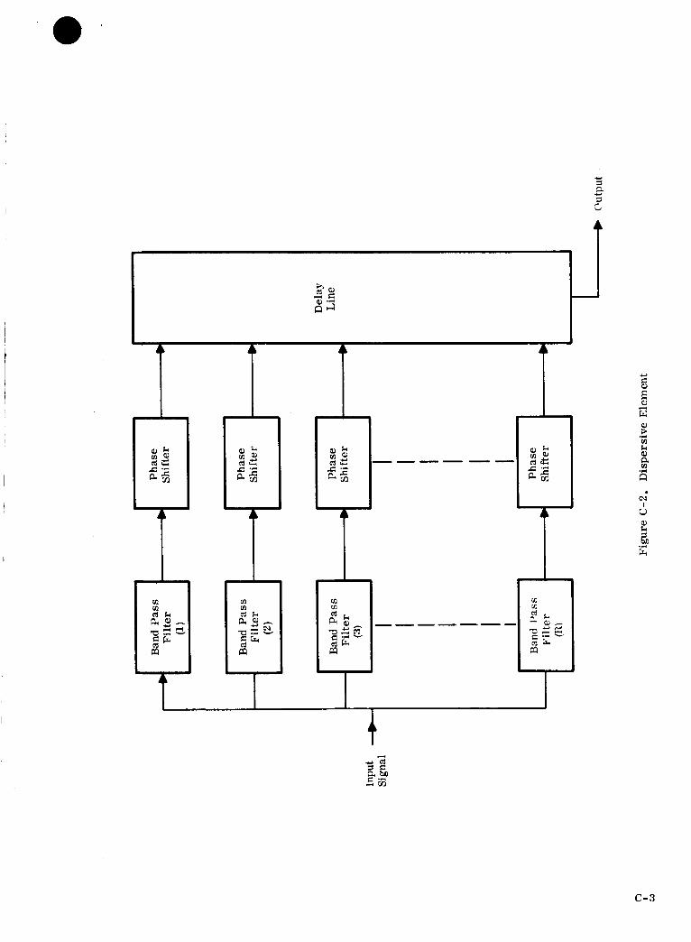
Lk & Lk

_k &I

Lk

r_

8I

Lk

Lk

C_

T_

I

C-3

Whenthe entire received signal has been applied to the filter band and the output arrives at the delay line

output, the energy will have been recombined into a short pulse of IF energy. The phase shifters, shown in

Figure C-2, areused to make fine adjustments of the delay line length to assure that the energy at the delay

line output adds in phase. It is necessary that the ratio of the center frequency of the filters to their band-

pass be such that, over the time of the trigger pulse width, there is not a significant loss of phase coherence

between the highest and lowest frequency.

Be PERFORMANCE ANALYSIS

To evaluate the trade-off performance of the system, some relationships must be defined. Let:

Bb = Total bandwidth occupied by the transmitted signal

Bf = Bandwidth of an individual filter, as shown in Figure C-2

R = Compression ratio = Bb/B f

t t = Width of trigger pulse (transmit mode)

t = Width of transmitted pulseP

t D -- Time required for detection of received signal.

It is assumed, here, that the delay line is so arranged, such that:

t

-_ = R . (c-l)tt

In consideration of the lower frequency allocations (VHF) and/or low cost user equipment, the signals

used for ranging are going to be bandwidth limited. As a result, in considering FM Pulse Compression, this

constraint requires the technique be considered in the light of limiting the total bandwidth for the transmitted

signals to be comparable to the bandwidth required by other modulation techniques. This is an unusual con-

straint for FM Pulse Compression.

The signal-to-noise ratio of the output of the FM Pulse Compression receiver can be assessed by

examining the dispersive elements. Assuming, for the moment, constant peak power transmitted, bothwith

and without compression, the signal voltage out of one of the filters should be the same as the signal voltage

out of a conventional receiver of the same gain and antenna capture area. The output noise of the filter,

however, will be diminished by 1/R. This assumes the same noise density in both receivers. Thus, the

voltage output signal-to-noise ratio of one of the filters is:

Vs _ Vs

(S/N)v - V = V " (c=2)n n

C-4

Further, itis assumed the FM Pulse Compression receiver is built so that the signal voltages from the

filters all add in phase at the end of the delay line, whenit is used as a receiver element. It is also assumed

that the noise voltages from the filters arrive at the end of the delay line in a totally uncorrelated fashion.

Under these conditions, the output of the delay line with respect to signal will be:

V s = R V s (c-3)o

Also, the uncorrelated noise voltage at the output of the delay line will be:

Vno (c-4)

where, Vnf is the noise output voltage of any one of the filters. Combining these terms, the total output signal-

to-noise voltage is:

R V Vs

(S/N)T V _ s - R " v'-r" .

Vnf n

Therefore, the output power signal-to-noise ratio is:

(c-5)

S/N = R 2 (S/N)p (c-6)

where, (S/N)pis the output power signal-to-noise ratio of the hypothetical single pulse receiver. Thus, the

peak power transmitted can be reduced by the factor R 2 for the same output signal-to-noise performance.

The FM Pulse Compression scheme, under the constant bandwidth constraint, also has its drawbacks.

Due to the matched filter processing, Woodward's relation can be used:

15_- -

(S/N)_ (c-7)

(which holds over a reasonable range of practical signal-to-noise ratio) and the factor 5r can be evaluated.

This factor is important, as itdirectly represents the measurement error achievable in the system. The

factor, B, in the relation, is the proportional to Bf of the FM Pulse Compression receiver; just as flis pro-

portional to B b of the "conventional" receiver.

Thus for the case of equal output signal-to-noise power ratio, the measurement error of the FM Pulse

Compression system will be R times that of the "conventional or single pulse" system. Within the range of

signal-to-noise ratios, where Woodward' s (1) relation holds, a trade-off between signal peak power and

measurement accuracy can be made. It must be recognized, however, that the error improves with the

square root of the power increase.

C-5

Another factor of system importance is the detection time. Since traffic handling capacity can be of

importance to the overall system, the time required for a detection (and range measurement) is an important

factor in the modulation technique performance.

Assuming the predetection filter shown in Figure C-2 acts in a fashion similar to a single section

filter, the output voltage will behave as:

e° = K' 1- e . (c-8)

For the case where the previously derived power advantage is not compromised in the power-accuracy

trade-off, the time a received signal must remain within the bandpass of a given filter is that time required

to allow the output voltage to rise to the detection threshold. Thus,

Kt

t D = _-- (c-9)

The required time is inversely proportional to the bandwidth involved. From this, a comparison of FM Pulse

Compression with the single pulse technique can be made:

%tD - Bf = R" . (c-10)c tDp tDp

In addition to the "dwell time" within a filter, the signal must traverse R filters; thus, the total detection

time is:

T D = R • RtDp = R 2 tDp . (c-11)

In this instance, if the accuracy penalty is held constant, a trade-off between dwell time and peak power can

be made. Since this trade-off does not affect the delay line length, the trade-off involves a decrease in

detection time, T D, with the square root of the peak power increase. Conversely, if the peak power is kept

high, a direct accuracy-detection time trade-off can be made. It is important to note that the full advantage

of reduced peak power comes only at the full sacrifice of accuracy and detection time.

The time figure of merit for the modulation technique, with respect to a single pulse technique, can be

evaluated as a function of R. For both the single pulse and FM Pulse Compression techniques, the message

length and detection times are very nearly one and the same. Thus, the intermixing factor:

Tp

M = TM + TA + TD + TG (2-4)

reduces to

Tp

M = TM + TA + TG . (c-12)

C-6

Furthermore, the acquisition time is nearly zero. Also, in both cases, the guard time, TG, probably

reaches a minimum near the value of one to three times the message length. So:

~ TpM

j TM (c-i 3)

where the factor J, accounting for message length plus guard time, probably ranges from two to four. From

the previous analysis, we can say that:

Mp

M c = R2 (c-I4)

where M c is the FM Pulse Compression factor and Mp is the factor for the single pulse technique. In both

techniques, there is not a significant amount of integration performed, in addition to the message length,

itself. Therefore:

T M ~ T M ~

= TM + TA + TD TM 1 .(c-15)

Thus, the data gathering efficiency is independent of the compression. The overall time figure of

merit for FM Pulse Compression is approximately:

FTp

FTC - R2 • (c-16)


In the usual implementation of a FM Pulse Compression modulation, the circuits of Figure C-2 are

inserted sequentially first in the transmit trigger channel and second in the receiver detection channel.

Toward the antenna end of the equipment, the signals in both the transmitter and receiver are amplified and

heterodyned to and from the proper operating frequency (Figure C-3). Thus, except for the somewhat

unusual transmitter technique of heterodyning to the operating frequency and amplifying to the desired power

level, the "extra" equipment necessary is as pictured in Figure C-2. In most cases, however, the FM

Pulse Compression technique has been used on "skin trackers." Here, however, a transponder at the user

site at least, is inserted in the transmission path. Thus, the earlier assumptions of the received signals

adding in phase at the output of the delay line must be examined carefully. One of the major reasons for

using the same circuits in the transmit channel and in the receive channel is to keep the received signal as

well controlled as possible in amplitude and phase. There are three possible cases to examine: (1) The

user equipment detects the received signal and constructs a similar transmit signal, (2) The user equip-

ment detects the received signal and transmits a different type of signal and, (3) The user equipment merely

frequency offsets the received signal and amplifies itfor retransmission.

C-7

©

00

.R

00

!o

13-8

In the first case, insomuch as the characteristics of the transmit dispersive element (Figure C-2) of

the satellite can be duplicated at each user, the full advantage of the trade-off functions can be realized at

the user receiver. While no data has been found on this particular aspect of the problem, the realization

can probably be near theoretical. With the small number of satellites that would be used, it is reasonable

to talk of having all satellite transmit dispersive elements very closely matched. Under these conditions,

the user receiver, when installed, could be phased properly when receiving satellite transmission and thus,

be properly phased for all satellites by a screwdriver adjustment.

On the return path, however, the satellite receiver must operate with literally thousands of user

transmitters. To expect that these user transmitters, in addition to being low cost, would all be precisely

matched to a common standard is unreasonable. This very real problem which would definitely degrade

performance, along with the realization that high peak power is not of as crucial a concern with the user

transmitter compared with the satellite, leads one to case two.

In this case the receiver situation for the user would be exactly as in case one. However, the

received pulse at the end of the delay line would be used to fire a simple pulse transmitter for return trans-

mission to the satellite. Thus, the FM Pulse Compression would only be used on the satellite-user down

link.

In the third case, theuser equipment would consist of a non-detecting receiver that would be used to

drive a mixer-amplifier for signal re-transmission. This is, of course, an attempt to make the user return

look like a frequency offset "skin return." In order to avoid degradation of the phase characteristics of the

signal, the receiver would probably have to be rather broad band. Unfortunately, if the receiver bandwidth

is broadened to minimize degradation of the transponded signal, the peak power saving is compromised.

Thus, the implementation trade-off here would be received bandwidth, satellite peak power and user return

transmitted noise. In this case, itmay well be worth while to have the user transmitted signal not completely

noise-free in order to ease the peak-power-bandwidth problem. Here, the satellite receiver processing is

relied upon to free the resultant ranging signal from noise.

From a preliminary look at the implementation problems, it appears that the second case is the most

desirable case.

With the second case of FM Pulse Compression on the satellite-user down link and single pulse on

the up link, it appears that some reasonable compromises have been made. The circuits of Figure C-2 are

additional items for the user receiver. The satellite peak power can be reduced. The user transmitter

and the user-satellite up link receiver can be simple pulse-type equipments. The user receiver and the

satellite-user down link transmitter will need to be R times better in frequency stability than for a single

pulse scheme. This stability criteria, however, with present state-ofTthe-art techniques is not a severe

constraint. For example, current typical specification, for aircraft receivers, require 20 parts per million

frequency stability, while one-half part per million oscillators without ovens, are readily available today.

C-9

One aspect of the use of FM Pulse Compression that must be recognized, however, is that the accuracy

suffers as peak power is reduced. This is true due to the fixed total bandwidth constraint. At VHF and low

UHF frequencies, the fixed total bandwidth is a real constraint due to the limited spectra available. It is,

also, atthese bandwidths and frequencies that a degradation in accuracy is least acceptable. Thus, the

application of FM Pulse Compression is most likely in the areas of the spectrum where bandwidths of 500

kHz and more are available. This is, fortunately, where peak power reduction is most needed.

C-10

APPENDIX D

FM-CW TRIANGULAR MODULATION


Frequency modulated-continuous wave triangular modulation radar is used in some radio altimeters.

It can provide high resolution at close range. As an example, the AN/APN-22 radar altimeter provides an

accuracy of _+2feet from 0 to 40 feet and an accuracy of _+5percent of altitude from 40 to 20, 000 feet. (Refer-

ence [13J .) Altitude of the aircraft is measured by sweeping a transmitted frequency back and forth between

two values. The frequency received back from ground reflection thus differs from the frequency being trans-

mitted by an amount proportional to the propagation time and, thus, the altitude of the aircraft.

The same concept may be applied to ranging from a satellite. A ground station transmits a signal that

is continually swept between two radio frequencies. The satellite translates the signal to a different carrier

frequency and retransmits it. The signal is transponded in a similar manner by the user, thence, back

through the satellite to the ground station.

The phase of the swept frequency modulation being received from the satellite is compared with that

being transmitted to yield the total distance from the ground terminal through the satellite to the user. The

known distance from the ground station to the satellite is subtracted to give the range from the satellite to

the user.

The relationships of the transmitted and received waveforms are shown in Figure D-1. As range

increases, the received signal is correspondingly delayed in time. Range is measured by heterodyning the

transmitted and received signals to produce a beat frequency, as shown in the lower part of Figure D-1. The

propagation time from the ground terminal to the user craft and return is so long that it is necessary to

sweep the frequency back and forth between itslimits several times during the propagation interval. This is

necessary in order to keep the bandwidth of the transmission within reasonable limits. The sweep rate must

be sufficiently high to give adequate range resolution. An ambiguity exists for each sweep cycle. If the

duration of the cycle can be made long enough, the ambiguity may be resolved by "a priori" information

about the approximate location of the user. However, the range resolution required, the sweep rate, and

hence the bandwidth of the signal are inter-related in such a way that the ambiguity interval may be too short

for a priori resolution. Two approaches to ambiguity resolution are recognized. In one apporach, it is

resolved in steps, starting with a long period for the sweep to provide a long ambiguity interval, but with

low range resolution. In subsequent steps, the period of sweep is shortened, locating the user in progressively

smaller range intervals, untilthe desired resolution is achieved. In the other method, a second modulating

waveform is superimposed on the frequency swept signal.

D-1

+

,-_ ¢q

'rime

Figure D-1. Transmit-Receive Waveforms


The FM-CW triangular modulation method does not impose any unique requirements on orbits or

satellite attitude stabilization. The satellite serves only as a signal relay at a reference point in space.

Its attitude does not affect the measurement, except, insofar as control of the attitude makes it possible to

improve the anterma gain and thus, reduce transmitter power both at the satellite and at the user.

1. POWER BUDGET

Power budgets are calculated for minimum signal-to-noise ratio and bandwidth. These are conven-

iently adaptable from those of Section IIIB for single pulse amplitude modulation. Referring to Table III-1,

Part L "power Delivered to User Receiver" is unchanged, as the same satellite configuration is assumed °

Only a few values of Part rl, "Receiver Power Required" are changed, as the same noise figures are

assumed.

The minimum signal-to-noise ratio in the BF bandwidth for the detection threshold of an FM receiver using

a hard limiter and no feedback is 9 db, in accordance with the following expression (Reference _4], page 55):

1/2_/_S t = 4k 1 (flfD)

St = rms carrier threshold

k 1 = rms noise voltage per unit bandwidth

flfD = bandwidth of an FM signal

(d-l)

D-2

hence:

Pt = Ski 2 fifD ; (d-2)

where, Pt = signal power at threshold.

Pt

k12 flfD= 8 : 9 db . (d-3)

In the example at the end of this section (Appendix D), the minimum bandwidth for 1000-foot range

resolution is calculated to be 4900 Hz, if doppler shift is negligible and the counting resolution is assumed to

be 4 Hz. For 100-foot resolution, using the same assumptions, the bandwidth is 15, 500 Hz.

The FM-CW triangular modulation power budgets for 100-foot range resolution are as shown in Table

D-1. The values allow 6 db above the detection threshold. Average power transmitted by the satellite is

the value indicated because the transmission is continuous.

Table D-1

Power Budget

I, Power Delivered to User Receiverdbw/watt radiation (into isotropicantenna)

II. Receiver Power RequiredReceiver Bandwidth Factor

(Change from Table III-1)

Receiver Noise Power (change fromTable 1TI-1 )

Desired C/N Ratio (change fromTable III-1)

>

DBW Required at User Receiver(actual -dbw)

III. Balancing the Budget

DBW/watt Radiated less dbw Requiredat Receiver

User Antenna Gain

Satellite Transmitted Power

Satellite Transmitted Power

dbw

db

dbw

watts

157 175

-4.8 -4.8

-4.8 -4.8

-5 -5

146.8 111.3

10.2 30.7

3 3

7.2 27.7

5.3 590

°,._ °,-4

• 0 •

172 182.5

-5 -5

190.5

-18.3

-5 -5 -18.3

-5 -5 -5

144.7 141.6 142.1

27.3 140.9 48.4

3 3 3

24.3 37.9 45.4

270 6200 54,000

D-3

Power values may be reduced in proportion to bandwidth for poorer range resolution. For 1000-

foot resolution, the power in watts may be reduced by the ratio 4, 900/15,500. Power budgets in Tables III-1

and D-1 assume user antennas With hemispheric coverage. If the beamwidth of the user's antenna is reduced,

the aperture becomes larger, and the satellite transmitter power requirement is reduced in accordance

with the curves of Figure IH-1.

Other detection methods may permit a reduction in power requirements. Feedback does not appear to

offer a large saving, however, as the noise bandwidth of a frequency modulation with feedback (FMFB) re-

ceiver is essentially that of the modulating waveform. As will be shown later, the modulating waveform

bandwidth is one-half the RF bandwidth when, P, the sweep period, is chosen for minimum bandwidth.

Hence, the saving with feedback would be less than 3 db.

Matched filter techniques might offer a substantial saving in noise bandwidth and a proportional saving

in power. A technique using comb filters was considered briefly. It would resolve range in discrete steps

and require matching the sweep period to the filter characteristics for each measurement. It did not appear

attractive because of its complexity and, therefore, it was not studied in detail.

2. DOPPLER EFFECTS

Frequency changes due to relative motion of the user, the satellite, and the ground station can cause

a frequency difference between the transmitted and received signals and, hence, a beat frequency. Figure

D- 2 shows the effect for doppler shifts to be smaller than r df/dt (where r is the time delay between transmitted

and received waveforms, and df/dt is the rate of change of frequency).

f2 + 6f

fl +Sf

/ ReceivedSignal Signal

0Time

Figure D-2, "Small" Doppler Effect

D-4

The average value of fb' the beat frequency between the transmitted and received waveforms over an

integral number of frequency sweep periods, is unchanged from the value without doppler shift.

On the other hand, if the doppler shift is greater than r df/dt, the average value is changed, as shown

in Figure D-3.

{:r

ft + 5f "___° __df

T_

f_

Time

Figure D-3° "Large" Doppler Effect

Doppler shift therefore, restricts the minimum T in the range interval so that

5fT > --

df

dt

where

5f = frequency shift due to doppler effect.

(d-4)

A convenient rule of thumb for one-way doppler shift is

one Hz/MHz/mach

(if "roach, " the speed of sound, is considered as 670 mph). Two-way doppler shift, as in an active ranging

system, will double the value.

Extreme cases for doppler shift occur when supersonic aircraft are on the horizon for the satellite

and moving directly toward or away from it° In the VHF aircraft band, the doppler shift of the signals for

a mach three aircraft can be as large as 820 Hz and in the 1540-1660 MHz band, as large as 10 kHz.

Doppler effects are a function of carrier frequency. Frequency sweep must be approximately twice

the maximum doppler in order to insure that a range measurement can be made without the doppler shift

exceeding T df/dt.

D-5

Other factors determining bandwidth are independent of carrier frequency. But doppler shift is not.

Hence the bandwidth at higher carrier frequencies may be determined primarily by doppler shift, if fast

aircraft are to be accommodated.

3. MULTIPLE ACCESS

As with other methods of range measurement, there are two factors that affect the multiple access

capability. These are:

a. Time for measurement and the capability for interleaving user interrogation during measurements.

b. The bandwidth required for the measurement.

The time for measurement is the sum of the address time, lock-up time, measurement time and guard time

between measurements. The total bandwidth required for the measurements must include the guard bands

between channels.

Users of the system may be interrogated in sequence or on separate radio frequency channels.

Propagation time from ground station through a synchronous satellite to a user and return is approxi-

mately one-half second. Several sweep cycles are needed to resolve the user's position within each ambiguity

interval. If no a priori information about the userVs range is available, the initial sweeps are 40 milliseconds

long. Between five and ten sweeps may be necessary to resolve the ambiguity, since several different slight

variations of the period must be sent in order to insure that the position of the interval in space places the

user in the favorable portion of the interval. (This is further discussed later in this section and illustrated

by Figure D-11.) The initial measurement takes at least several tenths of a second. While subsequent steps

in the position measurement use shorter sweep periods, the number is such that the total measurement time

will be between one and two seconds per user. Thus, the method does not compare favorably with some

other methods for time sequential multiple access.

The simultaneous measurement of a number of users on separate radio frequency channels is a possi-

bility. The bandwidth required for the measurement can be minimized, if the ambiguity interval is made

relatively short. However, an optimum system design may require a relatively large bandwidth and, thus,

limit the number of simultaneous measurements that can be made using frequency division multiple access.

4. GROWTH CAPACITY

Growth capacity is affected by both factors described for multiple access, and in addition, it is affected

by the energy required per measurement. Energy per measurement limits growth capacity because of the

limited amount of energy available in the satellite to supply additional channels. Since the transmissions are

continuous, the satellite transmitted power calculations in Table D-1 may be used to estimate satellite bus

power requirements for each channel. Bus to RF efficiency is in the range of 20 to 40 percent, depending on

frequency and transponder design. FM-CW triangular modulation is low in overall efficiency in comparison

with other methods; thus, it has a relatively poor growth capacity.

D-6

5. EQUIPMENTCONSIDERATIONS

Thereare no unusual requirements on equipment performance o Bandwidth and equipment stability

requirements are similar to those for other ranging methods. Signal propagation times through the various

equipments must be constant and known. It must not vary from one user's equipment to another by more

than the delay time allowed for the range measurement error attributable to that cause. Frequency stability

requirements for the transponders in the satellites and users are not unusually stringent. It is important

that the frequency stability be such that no more than one cycle of frequency change shall occur during the

time of measurement. As this measurement time is approximately 0.2 of a second, stability would be five

parts in 10s at 100 MHz or five parts in 109 at a thousand MHz. While this requires good frequency stability,

it is reasonable for operational equipments.

It is essential that the period of the triangular swept modulation be held very stably and be known very

accurately, sincethe modulation envelope is essentially a measuring scale in space. A frequency error will

cause a cumulative error along the length of the scale. It is reasonable to hold the error to approximately

one foot, sothat it will not contribute appreciably to the total error of the system. Such accuracy requires

that the frequency not change by more than one part in 65 million. Oscillators with a stability of one part

in 10 l° are readily available, sothat this equipment requirement is easily met.

6. PROPAGATION EFFECTS

There are no propagation effects unique to the FM-CW triangular modulation method of ranging.

atmospheric effects are as described in Section liE.

The

7. INTERFERENCE EFFECTS

Continuous wave interference within the passband of the satellite transponder will tend to capture a

portion of the satellite transmitted energy. Interference of this type was experienced during the initial

ground to air tests on VHF using the ATS-1 satellite. Transmissions from aircraft to the satellite on MHz

were subject to interference from unidentified, but probably legally operating sources. At times, the levelof

interference was large enough to capture enough of the 135.6 MHz down link power, so that the aircraft

transmissions were not relayed effectively. Interference of this type can be troublesome for a hard limited

transponder on a synchronous satellite because the satellite is in view of a large portion of the earth and,

therefore, of many potential interfering sources. On the other hand, the hard limited transponder is rela-

tively insensitive to impulsive type interference.

8. DETAILED PERFORMANCE ANALYSIS

The remainder of this section, on the performance analysis of FM-CW Triangular Modulation tech-

niques, is intendedto provide the analysis and derivations upon which the previous statements have been

based. It also discusses the ambiguity problem inherent in this type of modulation scheme.

D-7

iI

The maximum difference, or beat frequency, between the transmitted and received frequencies is

dffb max = _ r (d-5)

where r is the round trip delay time between transmitted and received signals. The maximum frequency

increases linearly with delay until the round trip delay time is equal to the time of the linear frequency

sweep in one direction. It then decreases linearly, becoming zero at the end of the triangular waveform

period. Ambiguity can be resolved within the triangular waveform period, P, by observing that, if T is less

than P/2, the increasing received frequency follows the increasing transmitted frequency. But, if r is greater

than P/2, the decreasing received frequency precedes the decreasing transmitted frequency.

The duration of the maximum frequency difference becomes a shorter portion of the sweep cycle, as

range is increased, untilthe round trip delay time equals P/2-the duration of the frequency excursion, i.e.,

one-half the sweep cycle. At that point, the maximum difference frequency is reached, but the time avail-

able for its measurement becomes zero. It is then more desirable to observe the average difference of the

transmitted and received frequencies over an integral number of sweep periods. Maximum and average

frequency differences as a function of range are plotted in Figure D-4.

b

Maximum fb as

range increases_

\ /

2 r 2 -

Increasing Transmitted Decreasing Received

Frequency Leads Increas- Frequency Leads Decreas-

ing Received Frequency by ing Transmitted Frequency

Less than Half Sweep Period. by Less than Half Sweep Period.

Time available for

J measuring maximum fb

Time

r : Two-way propagation time, or delay of received signal behindtransmitted signal.

P Sweep period.

Figure D-4. Frequency Difference Variation with Range

Average frequency difference, [fb Javg'

Figure D-4.

follows a parabolic curve as range is increased, as shown in

D-8

The pattern of average frequency versus range is repeated for every interval of range corresponding

to the two-way travel time in period P. For free space, there is a range ambiguity for every Pc/2 range

increment, where c is the velocity of light. Range measurement requires that the ambiguity increment must

not be shorter than the uncertainty in a priori knowledge of the user's range, or limits of range that can be

determined by another measurement, such as an additional modulation waveform on the signal.

When ranging from satellites, the desired accuracy of the range measurement may be high, and the

range differences between the nearest to the most distant users may be very great. For example, a syn-

chronous satellite system may require that ranges be measured to users anywhere between the subsatellite

point and the horizon. The total range from the satellite to the nearest and most distant users is, thus, be-

tween 19, 300 and 22, 500 nautical miles, respectively. The ambiguity interval is 3200 nautical miles. The

two-way propagation time for the ambiguity interval is 40 milliseconds; thus, requiring the P in the triangular

waveform modulation be at least that long if no other means is used to resolve the ambiguity.

Range accuracy of a practical navigation system must be a very small part of the total range ambiguity

interval. One way to achieve desired accuracy is to measure the range in steps, first locating the user to

a reasonably small part of the total interval, then within the smaller interval. The process is repeated in

several steps until the range has been determined to the desired accuracy.

It would be feasible to build a system in which the measurement resolution in units of P, An p, would

be in the range of 0.01 to 0.1 P. The first measurement will determine the range to /_lP, the second to

_2P, etc.

The measurement of AnP requires that average frequency over one modulation period be determined

to high accuracy. The resolution required in the measurement of average frequency is highest near the

mid-range because of the inflection in the slope of the parabolic relationship of average frequency and range

or period, as shown in Figure D-6. For a change of Ap centered at the midpoint of P, the change in average

frequency has a magnitude corresponding only to the change for AP/2 because of the inflection. It is also

the smallest value of change in average frequency for AP anywhere in P. It thus determines the change in

the measurement of average frequency that must be resolved in order to measure range to the desired

resolution. The expression for frequency counting resolution as a function of range, or period, is derived

below.

Given a signal which varies in frequency with time, as shown in the sketch below (solid line),

Time

Figure D-5. Sweep Frequency

D-9

the signal is to be compared with another signal with exactly the same frequency-time characteristics, but

delayed by a time r which is less than one period, P, of the original signal. This second signal is shown by

the dotted line in the following sketch:

{

Tim e

Figure D-6. Frequency Difference

The above figure shows the frequency difference of the two signals expressed as a positive number. The

average of the absolute value of the frequency difference I fb I avg' is the area under the curve in the figure,

divided by the base, P, or:

Ifb tav

simplifying:

T_P (d-6)

df ( r) (d-7)l_lav = _'a_ : - _ "

The expression is plotted in Figure D-7o Given the parabola of Figure D-7, partial differentiation yields:

A Ifb {av - dt 1 - AT . (d-S)

This equation is valid in the region given by

P Ar (d-9){_-- _} ->_

remembering that 0 _ r _-- P. But to be certain of the ends, let

Ar < r < P Ar (d-10)2 2

D-IO

Ifblav

I0 j_: T _ Time

P

Figure D-7. t fb t avg.

[ P[ < A r then our sampling with A rtakes _ fb [ avIf however T - _ -- 7-, to the peak of the parabola and

part-way down the other side. Thus, /x I fb Iav is the peak value of the parabola minus the lowest end of

the projection of the sample Ar upon the curve.

dfP r' dfll _- ]Ifb Iav = d-__ - _ - ' (d-ll)

d_[_ _, ___] (d-12)

when

D-11

and

T,=P IP i AT_ + _- T +--f- . (d-14)

If r and AT are expressed as fractions of P, values of I A I fb Iav I versus T for various AT aredf

given in Figures D-9 and D-10 in units of P _]_.

dfI fb I av is in units of P _. Reconsidering the original signal:

df

/,2_ P d-_

/ I

Figure D-8. A _fb I avg"

A{f {av--2 . (d-15)

In other words, to get A { fb { av as a multiple of the total frequency excursion of the original signal, its

numerical value, as determined by the equations on the previous pages, should be multiplied by two. Or

(p dr) = 2F(T)(_ dr) (d-16)A{ {av -- •

It is desirable to avoid using the center portion of the range ambiguity interval because Af bav is small

in that region. In order to resolve an increment of range, the change in Af bav must at least equal the

resolution of the counter that measures fb av" If the center portion of the ambiguity interval is used, thedf

total frequency excursion P _-_ becomes much larger than would be necessary if that portion were avoided.

As an example, if the range resolution is 0.05 P, Figure D-9 shows that the change in Af bav at the centerdf

of the interval is only 0.000625 P _ for an increment of range change. The total frequency sweep would

then have to be(1/6.25 x 10-_ Nor 1600N, where N is the counting resolution of the frequency counter. On

the other hand, if the portion of the interval between 0.46 and 0.54 of the interval is avoided, the minimum

Af. is 0.004 dfo a_l f P _]T' sothatthe frequency excursion is only 250N. Since the signal bandwidth is a function

of P _, there is a large saving in bandwidth by avoiding the use of the center of the ambiguity interval.

D-12

O

o

<1

0.020

0.015

0.010

0.005

\\

\\

\'\

\

0

0.4

\\\\

\\\

\\

\\\ \\\\

X\\_,'\\\\

0.0009

O. 000225i , I

iiII

//

/

//j //

//////Ii7 /

//i/"

,/-.-_/_/'/-,o.oo_

7 ] 1 0.000625, ,

0.5

i///.-

//.'/

T

0,6

T in Fractions of P

_" O.1P

0.06 P

0.05 P

0.03 P

Figure D-9. T in Fractions of P

D-13

A

0 .i0

0.09

0.08

0.07

t\\\t

_0o0\09

_9

>

0.05

<] 0.04

0.03

0.02

0.01

/

//\\ \

\ /

\ \\\ ///\ \\\ ///

"\\\t /#/,),\ I,il,t\X\ ,IZl

0.1 0.2 0.3 0.4 0.5 0.6 0.7

T in Fractions of P

Figure D-10. r in Fractions of P

//¢J�

/.///.

//

//

0.8 0.9

/

1.0

r=0.1 P

r = 0.06 P

r=0.05 P

T= 0.03 P

D-14

The ends of the interval, where _- is small, should also be avoided for two reasons. One is that fb

becomes vanishingly small as r approaches zero or P. But r must be large enough to provide a sufficient

number of cycles during the interval. The other reason for avoiding the ends of the interval is that r must

be large enough to accommodate doppler shift as explained previously.

Itis obvious thatthe center and ends ofthe ambiguity intervalcannot be avoided by ignoring range

intervals, for the user can be at any range from the satellite.Itis,therefore,necessary to avoid these por-

tions by shiftingthe intervalin space.

This can be done by changing P, the period of the sweep. The longest range ambiguity that must be

resolved is approximately the radius of the earth. A synchronous satellite is approximately six earth radii

from the earth's surface. The sweep period for resolving the largest ambiguity is thus one-seventh the

propagation time from the satellite to the limb of the earth; that is, to where the most distant user is located.

The ambiguity intervalmay be shiftedin range by one-fourth itslengthby changing the sweep period

by one twenty-eighth ofitsvalue. For shorterrange ambiguity intervals,the proportionate shiftin period is

smaller. Figure D-11 illustrateshow the ambiguity intervalis shiftedwith respect to a user's position.

User

Figure D-I1. Ambiguity IntervalShift

In the application of the method, there is no prior knowledge of the user's relative position in the

ambiguity interval, hence, a measurement must be made to determine if he is in a favorable part of the

interval. If he is, the measurement sequence proceeds to the next smaller interval. If not, the interval

must be shifted appropriately to place him in a favorable part. The test must be made for each successive

interval throughout the range measurement.

The measurement of range to the user requires that the sweep period be known accurately, for it is

in effect the calibrated unit of measurement on the distance scale. The accuracy of the positions of the

ambiguity intervals in space is determined by the timing accuracy of the frequency swept waveform.

To insure that the ambiguity interval limits are within the specified accuracy for the system, the fre-

quency of the modulating waveform must be known to within the ratio of range resolution to the total range.

Fortunately, the state-of-the-art in frequency measurement and control is such that the requirement is

easily met. The maximum range is approximately 1.3 x 108 feet. An accuracy of one part in 0.65 x 10 -8

would suffice for one foot resolution. The factor of two results because of the two-way propagation for active

D-15

ranging. Suitable oscillators are available as standard items. When the unfavorable parts of the ambiguity

interval are avoided by changing the period of the triangular sweep, the required frequency sweep is the

number of cycles that can be resolved by the counter, multiplied by the number of range resolution elements

in the sweep period. From this simple relationship, wecan derive an approximation to the signal bandwidth.

LetP

ambiguity interval =

range resolution interval = Ar

counting resolution = N

(N refers to the counting resolution of the counter, not to the stability of the reference oscillator. Counters

normally have a resolution of +1 count regardless of the number of events counted_ then the swept frequency

is

Pfs = N _ cycles . (d-17)

From Carson's rule for FM modulation, the bandwidth is the sum of the swept frequency plus twice

the highest modulating frequency, f. For a triangular waveshape, we approximate the modulating frequency

as three times the reciprocal of the triangular waveform period

~ 3 (d-18)

The transmitted signal bandwidth is:

fb _ N p 6 (d-19)w 2-Z'7 + _ "

The relationship of the terms in this expression are shown in Figure D-12. Approximating the highest

frequency component of the triangular waveform by fn = 3/P, implies that modulation sideband components higher

than the third harmonic will not be passed by the receiver. The effect is to introduce a small frequency modula-

tion component that averages out over a sweep cycle and also a small amount of amplitude modulation.

Minimum bandwidth may be determined by differentiating and setting to zero the expression for fbw"

Thus, minimum bandwidth occurs when

p2 = 120At (d-20)N "

Ambiguity must be resolved without excessive bandwidth. This may be done using the method described

previously, keeping bandwidth constant and using a difference _ for each step.

Another method is by the use of a second modulating waveform, superimposed on the transmitted wave-

form with a wave-length in space sufficient for the larger ambiguity interval. It may be sinusoidal in form.

This technique has been called double modulated FM (Reference 13 ). The envelope of the sinusoidal mod-

ulation is detected and the transmitted and received phases compared.

D-16

NP 6fbw := 2_ +

Minimum point

6

Ambiguity Interval

Figure D-12. Relationship of Ambiguity Interval and Bandwidth


Figures D-13 and D-14 are block diagrams of ground station, satellite and user equipments for the

FM-CW triangular modulation method. For illustration, we assume a system operating on VHF aeronautical

frequencies and a desired range resolution of one thousand feet.

A highly stable oscillator, preferably a cesium beam standard or a high stability quartz oscillator, is

suggested as the basic frequency reference. A cesium beam standard drifts approximately one part in 10 -11

during the life of the cesium beam tube; while a high stability quartz oscillator has a stability of approxi-

mately five parts in 10 -it per day. When used in a system in which the user transponds, frequency stability

of approximately one part in 10 -7 is required. However, if the system is to be used in a passive direct

ranging mode, as well-one in which the users receive signals and compare their modulation phase with an

on-board reference, the timing of the signals must be maintained to high accuracy with reference to stand-

ard time. The relatively small additional cost for providing the passive mode capability strongly suggests

that the high stability oscillator be furnished.

The output of the oscillator drives a clock pulse generator, thus, furnishing high accuracy timing for

the modulation phase. A ramp generator develops a triangular waveform that sweeps between two voltage

levels. The triangular waveform is applied to the modulator of the transmitter, so that the transmitted

frequency is swept linearly between two values.

D-17

Modulator

Clock

Pulse

Generator

RampGenerator

Counter,Time

IntervalPulse

Generator

AmbiguityInterval

Shift

Logic

/_VV

-- Coupler

t_ ransmitter] [i -_

FiTM

Figure D-13°

Synthesizer [

LStable

Gscillator

q p

Gate

[ i [ Co!te r

To Position

Fix Computer

Equipment Block Diagram

Diplexer

ntenna

Receiver

70 MHz

D-18

pd

_q

¢q

,-4

li![--

u_

O

D-19

Frequency sweep, counting resolution and range resolution at minimum bandwidth are related by

Equation (d-21).

p2 = 12A.___.__T (d-21)N

Ar = 2 x 10 -6 seconds for 1000 feet range resolution

N = 4 a value selected to allow for the _+1 count resolution of a normal counter plus possible false

or missed counts due to noise..

P = 2.45 x 10-_ (d-22)

The sweep frequency can be determined from Equation (d-17).

P (d-23)fs = N 2A---_

= 2450 Hz.

Doppler shift in the VHF aircraft band will not exceed approximately 800 Hz and, therefore, no addi-

tional allowance must be made to accommodate the shift.

Radio frequency bandwidth for the highest range resolution is the sum of both terms in Equation (d-19).

fbw = 2450 + 6 = 4900 Hz (d-24)2.45 x 10 -3

If the range to the user is completely unknown, he can be at any range from the subsatellite point to

the horizon; the initial triangular sweep period is 40 x 10 -3 seconds. The ramp generator, Figure D-13, is• P

adjusted to generate a voltage that will sweep the transmitter frequency 2450 Hz m _, or 20 x 10 -3 seconds.

The signal will be transponded by the satellite and user equipments. Each of the transponders is

designed to cancel the effects of drift in its local oscillator, byusingthe same frequency source for all fre-

quency translation. Doppler shift cannot be cancelled out by such a technique.

After approximately one-half second, the signal is returned from the user, and heterodyned with the

signal being transmitted to produce fb"

The ambiguity interval shift logic circuit resolves the ambiguity, causedby the increasing and decreas-

ing sweeps, by noting if the increasing received frequency follows the increasing transmitted frequency byp df

less than or more than _. It then observes the waveform to determine if doppler shift is larger than T

and also observes the average beat frequency to determine that it is below its maximum possible value-in2450

this case, _ or 1225 Hz. If one of the conditions is not met, the logic circuit shifts the period of the

sweep waveform appropriately so that the user' s range is within the acceptable portion of the ambiguity

interval.

D-20

Whenit has been established that the user is in the acceptable range, the Time Interval Pulse Gener-

ator opens the Gate and the beat frequency is counted over an integral number of frequency sweep intervals.

The total count is divided by the time of the counting interval to provide a measure of range within the

ambiguity limits.

Resolution depends on the location of the user within the ambiguity interval. As explained previously,

resolution is highest when the received frequency is close to the transmitting frequency, and decreases

linearly until the frequency difference approaches its maximum value. For the parameters selected, the

resolution will be in the range of 0.6 percent to approximately 5 percent, depending on where the user is

located in the interval. For 5 percent resolution, he is located to within 3200 x 0.05 = 160 nautical miles.

The sweep interval is then changed, but the magnitude of the frequency sweep is not. The sweep

interval, P, is longer than the two-way radio propagation time for the range interval, or

320P > _-_ x 10 -3 = 1.98 x 10 -3 seconds.

The measurement sequence, described above, is repeated for the new interval with the frequency sweep

remaining 2450 Hz. Range resolution is better than 0.05 x 160 = 8.0 nautical miles.

A third and fourth repetition of the process will locate the user within the desired 1000-foot resolution.

Four steps were needed because there was no a priori knowledge of the user's range and because the

user was assumed to be in the unfavorable portion of the ambiguity interval. In practice, it is unlikely that

four steps would be necessary;two, and, in some cases, onemay suffice for most measurements in an opera-

tional system, where the ranges are known approximately because they are measured frequently o

Numerous variations are possible in a system implementation. For example, the time for a range

measurement can be reduced, if the waveform transmitted from the ground station contains a sequence of

different sweep periods to insure that all the ambiguities are resolved, and that at least one sequence of

pulses in each ambiguity interval is proper for each possible location within the interval.

The basic user equipment is simple- consisting of a hard limited transponder. Its cost compares

favorably with that required for other modulation methods. It must receive and transmit simultaneously;

therefore, a diplexer is required. When the receive and transmit frequencies can be separated by approximately

10 percent, and wide bandwidth antennas are readily designed for the application, a diplexer can be provided

at reasonable cost. For aircraft at VHF frequencies, a diplexer may present a more serious problem, be-

cause it is difficult to design wide bandwidth antennas that are aerodynamically acceptable.

A discussion of the means that might be used for addressing users and for communicating, which might

be an important adjunct to the ranging function, has not been included. The communication functions can be

provided in essentially the same manner as in other modulation methods. Except for detection circuits,

there need be no essential differences in the address recognition, communication and display equipments.

D-21

APPENDIXE

PSEUDORANDOMCODETECHNIQUES

A. INTRODUCTION AND CODE GENERATION

In the past 10 years, there has been considerable effort on pseudo noise (PN} code application to com-

munications and to range measurements. This section of the report will draw from this work and analyze

properties of PN codes to determine their applicability for the system use, addressed by this study. Perhaps

one of the easiest ways to approach an explanation and analysis of PN codes is through the mechanics of

their generation. The ease with which these codes can be generated is one of the major reasons for their

wide application.

A pseudo noise sequence, or code, is generally generated from a binary shift register and logic cir-

cuit. The shift register is a series of digital flip flop circuits, that are arranged so as to shift a binary word

through the register in step with an applied train of "clock" or "shift" pulses. The individual stages of the

register, when triggered by a shift pulse, take the state of the previous stage in the previous bit time, as

shown in Figure E-1. Thus, the shift register can move a sequence through itself in exact synchronism

with a shift pulse train. To use a shift register to generate a code, itis necessary to use the output of the

register to provide the input through some suitable logic. One of the simplest forms of this logic has been

called by names, suchas "half adder" or modulo two "adder." This logic is most precisely described by the

"truth" table, shownin Figure E-2.

If the register of Figure E-1 were connected by half-adder logic, as shown in Figure E-3, the register,

when driven by a clock pulse train, would generate a sequence 255 bits long, without repeating. Looking at

the first line of the truth table of Figure E-2, notethe output of a half adder is a zero state if its inputs are

both zero. Thus, if the generator of Figure E-3 were set up with all zeros in the eight stages, this state

would never change. Should the eight stages be preset to any other configuration of ones and zeros, however,

as the clock or shift pulses drive the register, it would take on, successively, all possible states, except the

all zeros state. The serial sequence seen at the output would therefore, be a repetitive sequence 255 bits

long. Expressed mathematically, the sequence length is 2N-1 bits long; where N is the number of stages in

the shift register. Since 2N is the maximum number of different binary states N stages can possibly have,

and since the all-zero state must be excluded from the sequence, the value 2N-1 is a maximal length

sequence.

The logic arrangement, shownin Figure E-3, was picked specifically as an arrangement that will gen-

erate a maximal length code. The code generated is unique to the logic shown. Other logic or feedback,

configurations may or may not generate maximal length codes. The particular arrangement shown was

picked from a set of tables so that the sequence would be maximal length.

E-1

ClockorShift Pulses

Shift Register

_9

E

---_0

_9

O

O

---_0

Stage Stage .......... Stage1 2 8

*Numerals indicate the binary state of individual stages.

Figure E-1. Basic Shift Register Action

Figure E-4 shows cyclic diagrams depicting maximal and non-maximal length codes. In the reference

of these diagrams, the register, in generating a PN code, proceeds around the cycle of states the small

circles, each representing a particular state of the stages of the generator. The codes generated are cyclic

in nature. When a non-maximal length sequence is generated, there may also be other independent sequences

that can be generated by the same logic. The sequence generated can_ therefore, be dependent upon the state

from which the register starts. As indicated in the non-maximal length cycle A, there may be one or more

states that lead to a sequence, but which are never repeated once the sequence starts. By varying the length

of the register involved, the feedback logic and, perhaps, inthe case of non-maximal length codes, the initial

state of the register, codes of most any length can be generated.

E-2

Input A

Input B v Outout

Truth Table

Inputs

A B Out

0 0 0

0 1 1

1 0 1

1 1 0

Figure E-2. Truth Table and Logic Symbol for Half-Adder

8 Stage Shift Register

Output

Figure E-3. Sequence Generator (Pseudo Noise)

B. CODE PROPERTIES

In order to examine the application possibilities of the codes, it is helpful to look at some of the prop-

erties of the PN codes generated, as described. A property of major interest for PN codes is the auto

correlation function. Figure E-5 shows a plot of the autocorrelation function of a typical code. In this

case,At represents the time shift of the code with respect to an identical reference code. The autocorrela-

tion function, of course, repeats once per cycle period of the code. From the point of maximum correlation,

the function decreases linearly to complete loss of correlation in a one bit time space. Thus, the pseudo

noise codes are uniquely definable every bit period of their cyclic length.

E-3

2 3

2N_l

MaximalLengthSequence

Non-MaximalLengthSequences

FigureE-4. MaximalandNon-MaximalLengthSequences

E-4

Eventheshortest possible code may cause untenable acquisition times; therefore, acquisition short

cuts are desirable. A short cut analyzed in Para. H of this Appendix is to take advantage of the properties

of a code generated by a partitioned generator. As an example, assume a code of length 1 is made up of aP

logical combination of three sub codes of lengths 1K, 1M, and IN. The lengths of the sub codes will satisfy

the relation:

lp = OK) x (1M) x (IN) . (e-l)

The ',average length" of the sub codes will therefore be:

IAV = 3_]¢_p . (e-2)

If such a partition were physically realizable, the problem would then be to acquire three codes of length 1AV.

Taking advantage of the cross-correlationpeaks to trigger decision thresholds, the three codes can be

searched individually, acquiring first one sub-code, then another and finally the third to achieve full acquisi-

tion. Thus, only 3X (1AV) bit times need to be searched to acquire. In practice, itis often not possible to

realize exactly .3v/_-n as a code length; thus, the product of IK • IM • 1N is an approximation to the ideal.

In this case 1K + 1M + 1N bit times must be searched to acquire. The value 3 3_p is a lower bound on

maximum acquisition time and is not always exactly realizable. The value is, however, close to practical

results and a valuable estimation for a three part code, or more generally J J_, where J equals the num-

ber of sub-code lengths used.

D ° PSEUDO NOISE RECEIVER IMPLEMENTATION

Perhaps, themost common form of receiver for use with pseudo noise codes is shown in Figure E-6.

This receiver multiplies the received PN signal with a locally generated PN reference.

Input _ MixerSignal X H VCO ]

I

H Amplifter Detector Filter

t 1 r ns-Trans- l

mitter mitter

Shift PulseGenerator

Figure E-6. Pseudo Noise Receiver Implementation

E-6

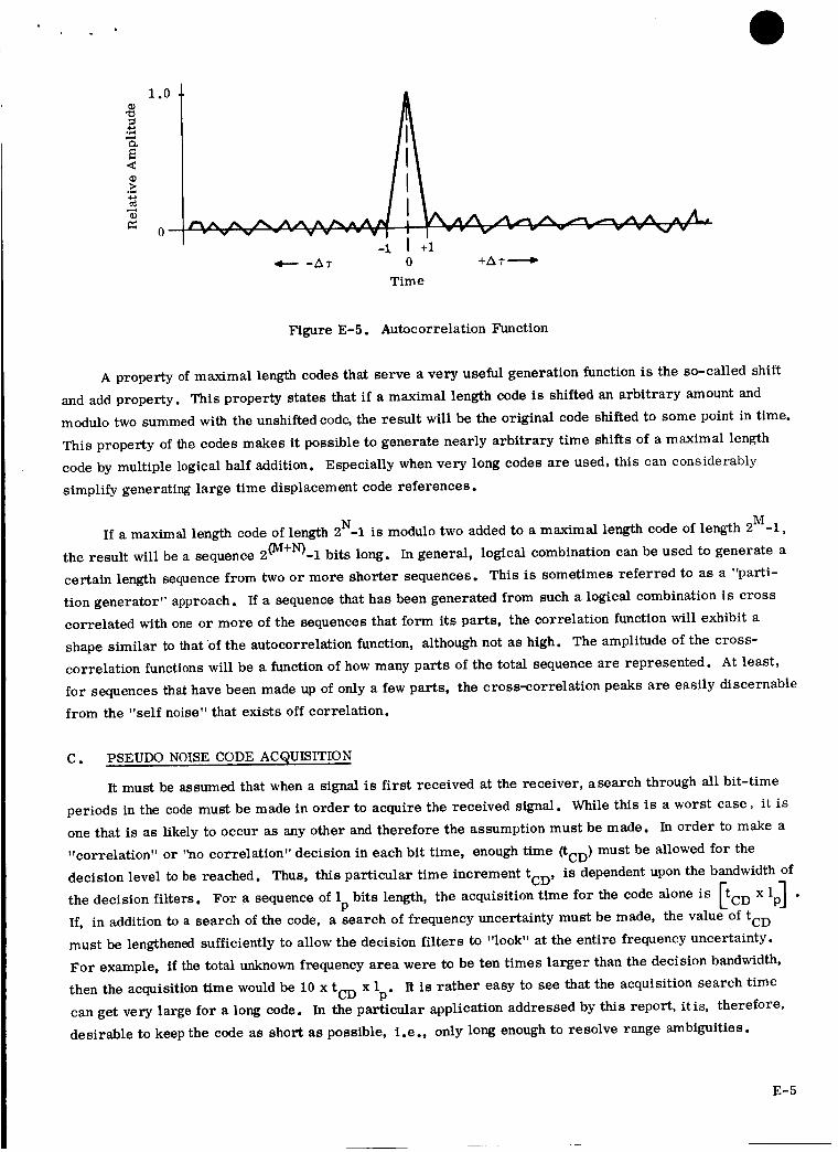
CD

°_

<O

?.c_

1.0

0 " v v _ " V v -v V{

-i-At

l v. V " v v v _ v _v

+1

+_ r'-_

Tim e

Figure E-5. Autocorrelation Function

A property of maximal length codes that serve a very useful generation function is the so-called shift

and add property. This property states that if a maximal length code is shifted an arbitrary amount and

modulo two summed with the unshifted code, the result will be the original code shifted to some point in time.

This property of the codes makes it possible to generate nearly arbitrary time shifts of a maximal length

code by multiple logical half addition. Especially when very long codes are used, this can considerably

simplify generating large time displacement code references.

If a maximal length code of length 2N-1 is modulo two added to a maximal length code of length 2M-1,

the result will be a sequence 2(M+N)-I bits long. In general, logical combination can be used to generate a

certain length sequence from two or more shorter sequences. This is sometimes referred to as a "parti-

tion generator" approach. If a sequence that has been generated from such a logical combination is cross

correlated with one or more of the sequences that form its parts, the correlation function will exhibit a

shape similar to that of the autocorrelation function, although not as high. The amplitude of the cross-

correlation functions will be a function of how many parts of the total sequence are represented. At least,

for sequences that have been made up of only a few parts, the cross-correlation peaks are easily discernablc

from the "self noise" that exists off correlation.

C. PSEUDO NOISE CODE ACQUISITION

It must be assumed that when a signal is first received at the receiver, asearch through all bit-time

periods in the code must be made in order to acquire the received signal. While this is a worst case, it is

one that is as likely to occur as any other and therefore the assumption must be made. In order to make a

"correlation" or "no correlation" decision in each bit time, enough time (tCD } must be allowed for the

decision level to be reached. Thus, this particular time increment tCD , is dependent upon the bandwidth,. -_°f

the decision filters. For a sequence of lp bits length, the acquisition time for the code alone is [ted x lpl o

L.

If, in addition to a search of the code, a search of frequency uncertainty must be made, the value of tCD

must be lengthened sufficiently to allow the decision filters to "look" at the entire frequency uncertainty.

For example, if the total unknown frequency area were to be ten times larger than the decision bandwidth,

then the acquisition time would be 10 x tCD x lp. It is rather easy to see that the acquisition search time

can get very large for a long code. In the particular application addressed by this report, itis, therefore,

desirable to keep the code as short as possible, i.e o, only long enough to resolve range ambiguities.

E-5

Assuming the two signals are correlated, the output of interest of the mixing process will be a spectral

line at the frequency difference of the received PN signal and the local reference. This signal is then

amplified and applied to a phase detector. In the phase detector, the correlated spectral line is compared

with a multiple of the VCO to develop a phase lock signal for the VCO. The VCO is also used to generate

shift pulses for the pseudo noise generator (PNG). This receiving approach assumes the transmitted PN

signal bit rate and carrier are phase coherent. Generally, a higher multiple of the VCO than the phase

detector reference is modulated to provide the first mixer reference. By means of removing or inserting

shift pulses, the PNG output can be shifted in time to mechanize a systematic time search for correlation.

Generally an output of the phase detector is used to sense correlation and stop the time search process when

full correlation has been achieved. If it is necessary to search out frequency uncertainties, this can be done

with a VCO sweep signal in conjunction with the shift pulse gating for time search. The receiver briefly

described here is of course, a basic phase locked receiver and can be analyzed as such.

In the succeeding sections of this Appendix, considerable analysis has been done to predict the per-

formance of PN codes to the application of this study. Based upon the results of this analysis, an example

is presented to illustrate possible performance of a pseudo noise system. The receiver of Figure E-6 is

assumed to derive its input signal from a standard VHF receiver IF. To maintain coherence, the LO of the

VHF receiver will be synthesized from the phase locked receiver VCO output. The phase detector operates

at 5 MHz. Since the phase locked receiver can be unlocked by noise, a signal-to-noise ratio in the loop of

10 db is assumed to be minimum allowable for consistent operation. While 6 db is generally considered to

be loop threshold for unlock, the probability of unlock, at this signal-to-noise ratio is quite high. For the

10 db signal-to-noise ratio, the phase jitter on the 5 MHz VCO derived signal can be calculated from the

phase error relation of Section V,

1S/N -

2 _E) 2 (e-3)

Ce - 1 = 0.5 _ 0.224 rad xl0

At 5 MHz, this corresponds to a time jitter of:

(e-4)

0.224x 1/5 x 1066T = 2_ = 7.1 nanoseconds (io). (e-5)

In practice, the receiver would be built with a 5 MHz oscillator, whichwould be divided to produce the de-

sired bit rate of 8 KHz. The division process generally does not reduce the time jitter. Therefore, the 7.1

nanosecond figure is a good estimate of the locally generated rms code jitter. This number is, of course,

much, much smaller than the other range errors that will occur at VHF and as such, can be ignored.

E. MEASUREMENT ACCURACIES

A major source of range measurement error for the pseudo-noise receiver is the receiver's ability

to locate the peak of the correlation function. As can be seen from the preceding discussion on phase lock,

the post-acquisition time jitter will be very small ; however, the acquisition accuracy must be treated

separately.

E-7

The accuracy with which the correlation function can be acquired is a function of the shape of the

correlation function of the pseudo noise signal. The shape of the correlation function is a triangle for

unfiltered pseudo noise; however, this is not the case for a filtered spectrum. As shown at the end of this

section, the equations for the autocorrelation function were derived for a spectrum filtered at the first

zero of the (sin x/x) 2 shape. This function was evaluated by the time share computer to obtain data on both

the autocorrelation function R(T)and its derivative R'(7). The data is included with the programs used to

generate the information. Figure E-7 shows the autocorrelation functions of the filtered and unfiltered

spectra.

Two approaches to acquisition of a PN correlation function have been popular. One approach is to

differentiate the output of a single correlator and use the result as a control function to position a servo

controlled local generator. Another approach is to use two correlators with their reference inputs dis-

placed in time relative to each other. This is done quite simply by tapping separate stages of the shift

register for the reference signals. The outputs of the two correlators are then differenced to yield a con-

trol function such as shown in Figure E-8.

With either approach, a servo control loop can be mechanized to center the local generator once the

code search has established some correlation between the local generator and the received signal. In both

cases, amplitude sensing of the correlation function must be used to sense acquisition and turn loop control

over to the VCO phase lock instead of correlation lock. In the case of the single correlator, the peak of

the correlation function must be sensed. For the double correlators the null of the differenced output can

be used. As can be seen in Figure E-7, the filtering process has rounded off the peak of the auto correla-

tion function. This makes the determination of the peak amplitude difficult, since the slope becomes so

small. Figure E-9 is based upon the slope of the autocorrelation function and is an estimate of the signal-

to-noise ratio required to make an acquisition decision to a given range accuracy. These curves ignore the

factors of frequency errors, amplitude errors, equipment drift and the like.

The coherent pseudo noise system can make very precise range measurements once phase lock is

established. The accuracy of those measurements, however, is a function of the accuracy of the acquisition

decision, basedupon the correlation function.

F. ACQUISITION TIME

A factor which has a major effect on actual acquisition time is the frequency errors that the system

must tolerate. As an illustrative example, assume one kilohertz frequency uncertainty and one watt trans-

mitted power. Using the second column of Table III-1, as a power budget, some calculations can be made.

For a phase locked loop signal-to-noise ratio of 10 db, the bandwidth factor would be: 42 - 27.5 =

14.5 db or 28.2 Hz closed loop noise bandwidth. AssumIng double correlators and 16,000-foot acquisition

accuracy, a 20 db acquisition circuit signal-to-noise ratio is necessary or a 2.8 Hz acquisition decision

filter (_D) .

E-8

]

r_

I

0

.!

0o

I

E-9

Figure E-8. Double Correlator Control Function

For initial correlation-no correlation decision, the output of the phase locked loop phase detector can

be used. As such, the frequency error can be searched out in accordance with the results of Section V.

Figure V-3 indicates a sweep rate of 100 Hz per second 2. Thus, ten seconds will be used to search out the

1.0 kHz frequency uncertainty per bit of code. For the 24 bits indicated in the analysis, aworst case time

of 240 seconds is necessary for establishment of correlation. For the 7 kHz bit rate being considered, the

16,000-foot range accuracy represents approximately 0.11 bit periods. Therefore, a search of nine time

slots may be required to establish full acquisition. The double correlator will have resolved plus or minus

limiting the search to one side of the control function of Figure E-8. For a 0.8/_ D time to decision per

time slot, this will require 7.2/2 x 2.8 seconds or 0.406 second. Thus, a worst case acquisition would take

240.4 seconds.

This acquisition time is very much a function of the received signal level. The curves for search rate

for a phase locked loop (Figure V-3) show:

SR = K _2

where

SR = sweep rate

Bn = closed loop noise bandwidth

K = constant depending uponlooptype, generally 0.1 -< K -< 0.16.

(e-6)

For a constant signal-to-noise ratio, the bandwidth is going to be directly related to transmitted power.

Therefore, the search time due to frequency uncertainty will vary inversely with the square of transmitted

power. Thus, 36 watts transmitted power could reduce the establishment of correlation to 40 seconds. The

time search for range accuracy acquisition varies inversely with bandwidth. Therefore the time search of

the correlation function would be 0.011 second. Of course, a direct time reduction can also be made by

limiting the frequency uncertainty.

E-10

v-_ N

//

/

0

0_9

¢D

J

/

A_r

/I

/

/

///

/!

//

qp - oT_H ogToN o'4 [_u_is po._TnbokI

17/I

i!/

ec_

¢x]

09

00

I

f_

¢.J0

t_0

¢/]

0

0

¢,J¢,J

0

,,..4

¢.J

I

E-II

G. SUMMARY

In a practical sense, pseudo noise codes require a relatively sophisticated receiver and can require

very long times for acquisition. Trade-offs of acquisition time for power can be made. However, if very

short times are a goal, the power required can get very high.

The range accuracy is a direct function of the bit rate used for the code. For low bit rates, rather

impractical signal-to-noise ratios for acquisition would be necessary. Time for signal-to-noise ratio trade-

offs can be made in this area also. However, this will only hold as long as circuit noise after the decision

filter remains small with respect to the noise out of the filter.

In general, PN codes appear to require too much time for acquisition and too costly a receiver for the

applications envisioned in this study.

H. DETAILED ANALYSES

i. FREQUENCY BAND OCCUPANCY AND INFORMATION TRANSFER RATE

In a pulsed communication system with fixed sampling rate, the power spectrum of the signal wave-

form is shaped for bandwidth economy. A major consideration is minimizing inter-symbol interference and

a minor consideration is reducing delay distortion. R is well-known that an ideal low-pass filter with a

cutoff frequency at 09v produces an impulse response of sin 09t/09vt type with uniformly spaced zeros at

t = k_/09 v. (Where k = _+1, 2..... } When sampled at the proper times, no inter-sample interference occurs

between such responses. But, because of the relatively large side lobes of this impulse response, errors

in the sampling times give rise to an intolerable residual inter-symbol interference. Furthermore, rela-

tively large delay variation associated with the sharp frequency cutoff of practical filters will time disperse

the response and enhance the inter-symbol interference.

According to theoretical results of Nyquist, the oscillating nature of the pulse tail can be reduced and

a more linear phase characteristic can be achieved by replacing this sharp cutoff by a more gradual cutoff

characteristic having even symmetry about the original cutoff frequency 09v" He has shown that such modi-

fication retains all the zero crossing points of the sin ¢Ovt/09vt type response and adds more zeros. In

particular, we may consider the raised cosine type spectrum for a low-pass filter; i.e., for some real

the even symmetric angular spectrum A(_ol) can be specifiedand 0 < 09 <X COV'parameters, u-- 1_o I - 09v

in terms of u as A*(u), thus

- sin _u/209v)1

A(I091) = A*(u) = E (1

o

-09 < U < -09V X

(e-7)lut -_ x

U > coX

E-12

The resulting impulse response of A(I co I) is given by Sunde (15) as

a(t)co sin co t cos co t

V V X

cotv [1- (2coxt/Tr)2 ]

(e-8)

Figure E-10 shows the normalized response with _x/co v as a parameter, for COx/cov = 1, 3/4, and 1/2.

With the reduction of COx/cov from unity to half, the maximum values of the side lobes of the response are

slightly increased, but the uniformly spaced zeros of a(t) are still spaced 7r/cov = 1/2f v apart.

A(tcol)1

cox=1

Cdx 1

_v 4

co

V2co V

a(t)

f

t _

Figure E-IO. Impulse Responses Obtainable with Various Sinusoidal Roll-Offs

E-13

For a signal transmitted through a time-varying medium, as long as the fading rate is relatively

small in comparison with the rate of information transfer, the time variation in the medium can be neg-

lected. The carrier phase can be determined at the receiver through a phase locked loop. In such a situa-

tion, it is highly desirable to use a product detector. The communication system is thus operated in a

phase-coherent mode with vestigial sideband-suppressed carrier transmission to minimize the frequency

band occupancy of the system. On a minimum bandwidth system, where only a single sideband is trans-

mitted, the rf spectrum occupies a frequency band from the carrier frequency ¢oc to an upper cutoff fre-

quency cod" Since such transmission characteristics involve a sharp cutoff at the carrier frequency coc' it

has all the drawbacks associated with the ideal low pass filter discussed before. On the other hand, a

vestigial symmetric case requires a slightly greater frequency band occupancy, butit allows a gradual filter

roll-off. By applying the Nyquist criterion used before, with the upper and lower sideband roll-off charac-

teristic matched to yield an odd symmetry about the carrier frequency ¢oc, the equivalent low-pass charac-

teristics of the system will be preserved.

= < cod - co " The bandpass angular fre-For some real parameters, let v I co I - coc and 0 < COy c

quency spectrum B(]co]), which has even symmetry about zero frequency, is defined in terms of B*(v) as

follow s:

B(}col) = B*(V)

<V <-co0 for -cov y

Try

1/2 (1 + sin_) Iv ]-<coy (e-9)

<V1 coy -<cod

,0 v >cod

N

When the low band-pass analogy is applied, the resultant angular frequency spectrum c(Ico I) of the

vestigial sideband system is defined as

(,col : B(,col [A(tu+ coet + A(lu- cocl ]

Recalling v = 1col - cod we can express c(lco I) in terms of v as c*(v), then

(e-10)

c(Icol) = c*(v)

0 for -co < v <-coc y

1/2(1 + sin_y) lv I-<coy

1

1/2 - sin _;

0

<V < coY- cocoy x

co -co _<V_<Co +cov x V x

v >coy +cox =cod

(e-ll)

E-14

where the zero frequency of the low pass characteristic A(1¢o I) is identified with the carrier frequency _c"

The corresponding double sideband characteristic c*(l_01) is the band-pass analog of B(]¢o I).

the linear sum c*(v) + c*(-v) which has even symmetry about v = O; therefore¢,

0 for Iv l>_ +_V X

Il_r(v+_v)]2_1/2 .+sin -_ - ¢_ -<v -<-_

V X VX

C(l_1)= _*(Ivl)= c*(v)+ c*(-v) =1

1/2 -sin 2_'x _v-_x_V-_W +_V X

The condition that assumes that the maximum response of c(_l) remains equal to unity is given by

-_ + u_ -----V _ -V X V x

It should equal

X

(e-12)

_x + _y -< _v = _d - _x " (e-13)

2_x

For the case of utmost symmetry whenX

-<_v°r_x-_v/2"-

= _y, the above relation is reduced into _ + ¢_ =x y

Then, inthe expression of c(_]),the true B(I_I) A (_u + _ ]) has even symmetry with respect toC

- (_c + _v/2) and the term B(]_I) A (_ - _c l) has similar even symmetry with respect to _c + _v/2" If we

also let_ = _ = _ /2, andx y v

_J

v _ ]_ 1 - _ - _ , (e-14)W = _] - _C 2 C X

the band-pass characteristic will have even symmetry with respect to its band center frequency w = 0, and

we may rewrite c(] _1) in terms of w as c(lwl)

c(l_I) = 3(twl)

Ii/2 1 - sin for iw I -< _ 1

( x= x (e-15)

0 Tw I>_o .X

According to analysis by Sunde (15), such a roll-off characteristic is one of those closest to a linear

phase characteristic as shown in Figure E-11. Therefore, it will only introduce negligible delay distortion.

All the spectra discussed above are shown in Figure E-12.

E-15

I_N_ i / Sinusoidal

"Anear_ Roll-Off

0 ¢o 2_V V

Figure E-11. Cross Approximation of the Sinusoidal Roll-Off Lowpass Filter

Characteristic to the Linear Phase Lowpass Filter Characteristic

2e SIGNAL-TO-NOISE RATIO AND FREQUENCY BAND OCCUPANCY FOR VARIOUS MODES OF

TRANSMISSION

If a modulating signal v(t) modulates a sinusoidal carrier A cos _o t by amplitude modulation, thec

modulated signal s(t) can be expressed as

s(t) = A _1 + v(t)] cos _c t . (e-16)

But if a balanced modulator is used to suppress the carrier, then the resulting double sideband signal

s2(t ) is given as

s2(t ) = Av2(t ) cos ¢Oct .

Let v2(t ) = cos ¢o t, then,X

s2(t ) = Acos ¢OxtCOS¢O t = A A __x)tc _ cos @c + ¢°x)t + _ cos (¢oc

If a high pass filter with cutoff frequency ¢oc

signal is given as

(e-I7)

• (e-18)

is used to remove the lower sideband, then the single sideband

sl(t ) = Avl(t ) cos ¢Oct . (e-19)

Suppose we let vl(t ) =_-cos ¢Oxt, then, after extracting the lower sideband, we obtain

A (e-20)

st(t ) = _ cos (co c - COx)t .

The peak power, A2/2, of the double sideband signal s2(t ) is reached when both sidebands reach their peak

power together. But the single side signal sl(t ) also has a peak power of A2/2. Thus, sl(t ) and s2(t ) have

identical transmitting peak power.

E-16

/ I0

A(t_l)

LOV

u=O U=_X

-COC

/

i lC

v=O V=_

Y

,!,-_c 0 coc _d

B(J_l) v=0 v= w v=_ v-_ +wy v v x

C

/.J

= i/2X V

=_ =1/2 coX y V

B(f_1)

v=0

A(I_])

co co=0 _dC

v=O V=CO V=_X V V=_v _ COX

CO _ _ + COX V V X

Figure E-12. Various Spectra

E-17

When a product detector with local oscillator voltage K m cos ¢Oct is used to demodulate either the

double or single sideband signal, the recovered signals r2(t ) and rl(t ) respectively, are given as

AK AK AK

rn t+--_ cos (2co +cox) t + mr2(t ) = Kms2(t ) cos coc t = _ cos cox c _ cos (2coc - cox)t (e- 21)

AK AK

rl(t) = Kmsl(t) coS_Oct = 2---_ cOS_xt + _cos (2Wc-C_x)t .

After passing through an ideal low-pass filter with cutoff frequency co ,when coV V

outputs r2(t ) and r_(t), respectively, are given as

> O_X_

(e-22)

the resultant baseband

AK m

r2(t ) = --_ cos coxt . (e-23)

AKm

= -- t (e-24)Xrl(t) 2/'2 cos ¢o ,

-v

where the peak power of the recovered baseband signal for a double sideband system is exactly twice the

corresponding peak power of a single sideband system.

If stationary white Gaussian noise n(t) is associated with the transmitted signal for either s2(t ) or sl(t )

with power per unit bandwidth given as No, then n(t) has a uniform power density of No/4_ per radian from

= -co to oo.

Since we are only interested in narrow band communication systems, we may replace the white noise

n(t) by a corresponding narrow band noise process expressed as

n(t) = nc(t ) cOS_ct - ns(t ) sincoct , (e-25)

where both nc(t ) and ns(t ) are stationary, white, Gaussiannoise with identical power density per unit band-

width as n(t). Thus, the demodulated noise output from the product detector rn(t ) is given as

Kmnc(t) Kmnc(t) t Kmns(t) sin 2¢0 t (e-26)rn(t) - 2 + 2 cos 2coc 2 c "

¢o < 2co c, the baseband noiseAfter passing through an ideal low pass filter with cutoff frequency _v' v

process rn(t ) is given as

Kmn c (t)

rn(t) = 2 " (e-27)

If the receiver filter has a transfer function H(co), the mean square output noise power (_N 2 is given as

qN 2 = --Kin4E = __m167r° H (I¢oi) 2d_o = m8_ o H (I¢oi) d¢o . (e-28)

--oo O

E-18

For the double sideband signal, the ideal bandpass filter IH2(1_ D

I 1 for I_-_ 1 -_

l 1 °H2(_ )

0 T_-_c 1 >_v '

t I'and for the single sideband signal, I-I1 (I_1) is specified by

,2{ 0t HI(_) = 1

0

for _ - _ < 0c

0 -_ _ - _ <_c v

c v

Therefore,

_is specified by

}(e-29)

(e-30)

K 2N f K 2N f(y 2 : m o v and 2 - m o vN 2 2 ¢YN1 4 (e-31)

The corresponding peak signal-to-mean square noise power ratios P2 and Pl for double and single

sideband systems, respectively, are given by

A2K 2m

4 A 2P2 =

K 2N f 2N_m ov ov

2

(e-32)

A 2 K 2m

8 A 2Pl = =

K 2N f 2Nf 'm O V OV

4

wheref = C_v/2_. It is clear thatpl = P2 = P.

(e-33)

If we use a gradual roll-off filter instead of using an ideal bandpass filter, for the double sideband

system, and also minimize inter-symbol interference, the previous analysis shows that the desired recov-

ered signal spectrum is givenby Equation (e-8}. The corresponding bandpass characteristic for the case

2C_x = c_v is given by Equation (e-12) as Cv(lC_ I). According to the matched filter theory for minimizing the

interference caused by added Gaussian noise, the transmitting and receiving filter must have conjugate

spectra so that

I H2"(¢_) I = _1 * (e-34)

E-19

Then the power spectrum of the receiving filter is given by

t H2"(lc°1) I 2 = Cv(I o_ !)

and

(e-35)

(e-36)

Similarly, for the vestigial sideband case, when the desired bandpass characteristic is specified by Equation

(e-15)asc_l). Also according to matched filter theory, the receiving filter spectrum is

The power spectrum of the receiving filter is given by

and

I Ht*(l¢°]) I 2 = c(_]) , (e-38)

(e-39)

Therefore, the peak signal-to-mean-square-noise-power ratio for the double sideband gradual roll-off case

and vestigial sideband case are given as P2* and Pt*, respectively, and

A2

P = 02* = Pt* = 2N--N-'-t_ " (e-40)O V

Therefore, the four different coherent systems, discussed, allhave identical information transfer rates and

identical peak signal-to-mean-square-noise power ratios, p. Their only difference is the frequency band

occupancy.

The vestigial sideband system is chosen as an engineering compromise because of its smaller fre-

quency band occupancy and lower sidelobe response. In the subsequent analysis, it is more convenient to

determine signal-to-noise ratios on the basis of the double sideband system.

3. MULTIPLEXING SPEECH AND RANGING CHANNELS AND RANGE DETERMINATION

We next consider a particular communication system, in which two channels are multiplexed together--

one channel for speech transmission and the other for ranging by a eontinuou_ waveform. The speech

channel requires an information transfer rate of 7 x i0 3 pulses per second to avoid any sacrifice of its

quality. We assume the ranging channel can handle the same information transfer rate theoretically. But

in practice, its critical rate of information transfer may be much slower. Therefore, the total information

transfer rate of the combined communication system is assigned a rate of 1.4 x 10 4 bits per second.

E-20

According to the previous analysis in this section, if a coherent system with vestigial sideband transmis-

sion is adopted, a frequency band occupancy of 1.4 x 104 Hertz is adequate. We will consider both time

division multiplex, TDX, and frequency division multiplex, FDX, for multiplexing the two channels.

For coherent transmission with limited frequency band occupancy, the speech signals are most

efficiently transmitted by bi-polar pulse amplitude modulation. Because such a system has a suppressed

carrier, it need not transmit any pulses at all during pauses in speech. Thus, it achieves an important

energy saving for satellite application.

Because the two channels are multiplexed together, the speech channel is always available except for

the small portion of time set aside for user identification signals. The ranging channel contains a contin-

uous sequentially modulated waveform, originated at the ground station. The userts equipment automatically

transponds the ranging signal. Ranging and speech signals from the ground station are relayed from the

satellite and demultiplexed in the userWs receiver. The received ranging signal is multiplexed with the

user's speech signal and shifted to a different frequency to be rebroadcast toward the satellite for relay to

the ground station. Range determination is made at ground station. The total round trip delay rd is ex-

pressed in terms of discrete phase or number of bit intervals m i, a positive interger, and 0 the vernier

phase is a positive realconstant, 0 -< 0 -< 2_, that is

rd = m i + _-_ d r , (e-41)

where, d r = 1/f v is the bit duration or interval, and fv = Fo/k v, where 1% is a positive integer and F ° is the

frequency band occupancy of the combined communication system. The range accuracy is determined by

the accuracy of the vernier phase, 0, which is determined by a phase locked loop.

The variance of range error ¢ 2 in the direction of a unit vector u, thatlies on the straight line joiningr

the user and satellite, is

2 C2_r = _02dr 2 _ , (e-42)

where a02 is the variance of the vernier phase error 0c and c is the velocity of an electromagnetic wave.

The variance _d 2 of the actual range error is the projection of ar2 onto the user's horizon in the case of

an aircraft, its artificial horizon. Let h be a unit vector in the direction determined by the intersection of

the plane of incidence of the electro-magnetic wave and the user's artificial horizon. Then, the cosine of

the angle • between u and h is given by l u • h _ and we have

= • c2_02 dr2 _ . (e-43)

The signal-to-noise ratio is least at the edge of the coverage, and at the same time, the vector _ almost

lies on the user' s artificial horizon; that is I-u • h I _ 1, and ad 2 _ _r 2, so that this case results in the

maximum range error.

E-21

4. MODULATION BY BINARY SEQUENCE FOR RANGING AND ACQUISITION TIME

Ifthe ranging system must cover a long unambiguous time interval T, the transmitted signal must

equal or be larger than T. If such a signal s(t) is to be generated by a binary sequence v(t), modulating a

sinusoidal carrier wave of angular frequency ¢oc by amplitude modulation, the relation between s(t) and v(t)

is given by

s(t) = A [1 + v(t)] cos ¢Oct. (e-44)

But if a balanced modulator is used to suppress the carrier, then

s(t) = Av(t) cos ¢Oct. (e-45)

Now if v(t) is a binary sequence having the values +1 and -1, clearly

+_ cos ¢Oct for v(t) = +1 1

s(t) = (e-46)

- cos _ t v(t) = -Ic

The waveform of such a signal is called phase shift keying where the phase is shifted by 7r radians

between the '_nark,' and "space" of the modulation signal.

Let fc = ¢°c/27r' andletthe binary sequence have a bit-rate of f bits per second, then, for the case of

coherent transmission, the carrier frequency fc must be an integral multiple of the bit-rate fv" According

to the previous analysis for the product detector, the frequency band occupancy is equal to the bit-rate of

information transfer. Therefore, thebit duration of the binary sequence is given by

d = __1 (e-47)r f "

v

Now if such system is time multiplexed into two channels, one of which is for ranging and the other

for speech transmission, the length of the ranging binary sequence must be _ bits long such that

> T (e-48)-_--_ .

In the receiver, the component of greatest concern is the product detector. If the two inputs to the

product detector are PSK signals of identical bit duration, as described before,

Sc(t ) = A cVc(t ) coS(_c t + 0c)

sb(t ) = Ab Vb(t ) cos (_b t + 0b)

(e-49)

(e-50)

E-22

then,theresponseof theproductdetectoris

AcAbK m

r <t)-- 2 Vc )Vb< )cos coc-copt ÷ (0c - °0]

AcAbK m

2 Vc(t } Vb(t ) cos _¢o c + ¢ob)t + (0e + 0b)]

where K m is the net gain through the product detector.

I (e-51

If one of the sidebands (say the upper one) is removed by a linear filter, and the resultant response

r(t) and the bit duration between the two input signals has been synchronized, (i.e., Oc - Ob = 0), then

AcAbKm 1r(t) = 2 Vc(t ) Vb(t ) cos (¢oc - ¢ob)t = A Vl(t ) cos (coc - ¢°b)t (e-52

where q

Ac% A = 2 and Vl(t ) = V(t) Vb(t ) (e-53'

Since Vc(t ) and Vb(t ) are binary sequences, Vl(t ) must also be a binary sequence, which takes on the values

+1 or -1, accordingto the following Karnaugh chart

V b {t)

+1 -1

+I +i -I

V c (t)-1 -1 +1

It is interesting to note that, if a very narrow bandpass filter has its center frequency at angular fre-

quency coc - C°b' it will integrate r(t). If both Vc(t ) and Vb(t ) have period T, then the sampled output of the

narrow bandpass filter, after multiplication by cos (coc - cob )t in a product detector, is the correlator output

for two input modulated sequences, as shown in Figure E-13.

V c t(t) cos coc

Narrow BandSampler

v[ Filter [--_

¢Vb(t ) cos ¢obt Samplingclock

Correlation

Function

Indicator

cos (coc - _b ) t

Figure E-13. The Correlator of Two Binary Sequence Modulated Waveforms

E-23

A

We now define acquisition time, Tac q, as the time required for determining the discrete phase m i orthe exact number of bits thatthe received sequence has been shifted relative to the transmitted sequence. For

any long sequence with a two level correlation function, such a determination can be made by selecting the

peak output among all the outputs of a set of correlators whose reference sequences consist of every possi-

ble shifted version of the transmitted sequence • If an integrator takes k bit-durations to quench after samp-

ling before it is ready for the next integration, and the total number of correlators in the receiver is h, then

^ £ + k)drTacq h ' (e-54)

is a good measure of the acquisition time• It is obvious Tae q is proportional to_2• The integer k is

usually small compared with 1. Therefore, for a single receiver having a single correlator, Tac q _ IT.

In order to reduce Tac q, the most obvious solution is to increase the number of correlators in thereceiver. But for long unambiguous range, _ is large, and we would need hundreds of correlators before

Tac q would be reduced to a practical value. An alternate way to achieve the same goal has been proposed

by Golomb (16) and realized by Easterling (17)• It has been successfully applied in spacecraft ranging sys-

tems. Since our pKoblem is similar to the spacecraft ranging problem, a slightly modified version of this

ranging system will be discussed in detail •

An apparent difficulty of binary correlator receivers is that simplicity can only be achieved with long

acquisition time • This may be remedied, however, by adopting a composite sequence formed from many

shorter sequences • For instance, if several sequences all have different periods, such that the common

factor between any pair of periods is unity, then the common period of the composite sequence must be

equal to the product of the periods of the component sequences• If a total of J component sequences is used

to form a composite sequence in this way, the approximate period of component sequences is only the jth_

root of the period of the composite sequence. Then, according to the Chinese remainder theory (reference

1181) which states that

every system of linear congruence

X 1 = C1 rood _ 1

x.

] = cj mod_j

in which the moduli _j (1 < j -_ J) are pair wise relative prime,

is the product of all the moduli in the system, i.e.

is solvable,

(e-55)

and the modulus solution x

JJ

x : crood_llej: croodZj:l

(e-56)

P E-24i

Therefore,the _ discrete phases of the composite sequence is uniquely specified by a J-triple vector

cj _ - -c = (c 1..... ), cj nod j for 1 < j <J,

the set of discrete-phases of all component sequences.

ranging system, using such a composite sequence, is

(e-57)

Therefore, the approximate acquisition time of a

(_-_ _j/(_+k) d rT J = _=1 ~ J l 1/J(l + k) d r

acq h h (e-58)

But the ranging system, using composite sequences,.requires a frequency band occupancy J times the original

frequencyband oceupency, because now J component sequences must be transmitted in parallel.

5. BINARY SEQUENCES THAT ARE GENERATED BY BOOLEAN FUNCTION OF COMPONENTSEQUENCES AND THEIR CORRELATION FUNCTIONS

In a pseudo-random sequence of length _ (_odd), there are (_- 1)/2 minus ones and (_ $ 1)/2 plus

ones or vice versa. We assume here that the first case is true, and fromnowon, we use the notation'" "+"

for "+1" and "-" for "-1." The relative frequencies with which the sequence assumes the individual value

+ or - are then given by

P(-) =

p(+) = (_+I) (e-59)2

Two sequences with relative prime periods, _i and _2, respectively, [i.e., (21, _2) =i] , take on all

possible discrete phases with respect to each other during the combined period _ = 1112. Knowing the

phase of either sequence does not give any information concerning the other sequence. If we state this con-

dition differently, we consider the sampling of two sequences randomly. The occurrence of a particular digit

in one sequence does not affect the probability of the corresponding digit in the other sequence. Thus, we

are assured that the two sequences of mutually prime periods are mutually independent statistically. We

may use this property to compute various in-phase and out-of-phase correlation functions between sequences.

For example, we may choose the first sequenceX: {+++-+--} and the second sequenceY: {++-}.

The relative frequency of the value + or -, occurring in the X and Y sequence, are given as

_) = 3 1

7

X (e-60)

(.p(+) = 47 "

1

y_P(-) = 3 }2 (e-61)

kp(+) = .

E-25

Then the joint relative frequencies of certain XY pairs occurring in the correlator are

3 1 3p(-,-) = _x _ _ 2-Y

3 2 6p(-,+) = _ x _ = 2-Y

4 1 4p(+,-) = _ x _ = 2"-]"

4 2 8p(+,+) = _ x 3 - 21

(e-62)

The above states of the auto-correlation function can be represented by the Karnaugh graph, where the

resultant state is the product of the corresponding states in X and Y sequences as shown below at the left,

and the corresponding joint relative frequencies are as show below at the right.

Y

+

1

2

X X3

321

6

4

421

821

The relative frequency of bits between X and Y sequences, being in agreement, is the sum, of the joint

relative frequencies of all the states denoted + in the left square, and the relative frequency of bits in dis-

agreement is the sum of the joint relative frequencies of all the states denoted by - in the left square.

Therefore, the normalized correlation function Pxy(J ) , according to the formula given in Equation (e-62), isas follows

1Pxy (j) = P(+' +) + P(-'-) - P(-'+) - P(+'-) = 2-'_ j mod _ . (e-63)

Such a Boolean sequence, formed bythe Boolean function of two or more sequences, digit by digit, has the

desired properties for ranging. Although it has multiple peaks in its auto-correlation function, the sub-

peaks may be used for the alignment of component sequences. In particular, the most important properties

of the composite sequence are: 1) the number of occurrences of + or - must be balanced; and 2) there should

be a dominating sequence such that in the auto-correlation function, the sub-peak only occurs when the dom-

inating component sequence is in phase. If only one non-dominating sequence is in phase or only several

non-dominating sequences are in-phase at the same time, the correlation function must remain at small

value.

Eastering gives such a Boolean function for three component sequences, X, Y and Z, when X is the

dominating component sequence. The Boolean sequence U is defined by

Y -- x (r_ z). (e-64)

E-26

where, all.the component sequences are pseudo random sequences, having mutually prime periods _ x' _ y and

lz. The period of U is _ = lxiylz"

The "AND" ("OR") logic used to combine the sequences Y and Z and the product ("AND") logic used to

combine X and (Y & X) are given by the following Karnaugh graphs.

Y Y&Z

- + - +

Z X

+ - + + - +

"OR" "AND"

Every possible state of this Boolean sequence is given by

Z - + ÷ - - + + -

y - - + + + + - -

(Y&Z) - - + +

X + + + +

U + + - + - + - _

(e-65)

The computations of the correlation function of binary Boolean sequences with pseudo random sequences as

components are much simplified by assuming the component sequences to have an equal number of +'s and

-'s--the longer the sequence period, the better the approximation. Under such an approximation, when

computing the auto-correlation function of U and u (where the lower case letter is used to differentiate the

out-of-phase version of the same sequence denoted by the capital letter), the following four different situa-

tions between corresponding values of U and u occur equally often:

(-, -) (-, +) (+, -) and (+, +) .

Since the particular Boolean function, specified U, is symmetric in Y and Z, we note, in computing the

correlationof U and u. that the correlation with the Y component alone in phase must be identical with the

correlation with the Z component alone in phase, and the correlation with X and Y components in phase must

be identical with the correlation with X and Z components in phase. In computing the correlation, we list

every possible state of U and u sequences on adjoining sides of a square; then in every element of the square

matrix, if the column state is in agreement with the row state, + is entered, otherwise - is entered. The

number of + and - entires in the square matrix must now be counted. The out-of-phase correlation is

easily computed in this way, for each entry occurs equally often. When some components of the sequenc_

are in phase, certain combinations of states in the square matrix become forbidden states. If we shade all

of these forbidden states, the correlation can be found by counting the number of agreements and disagree-

ments in the remaining unshaded squares of the square matrix. In Figure E-14, we have determined the

auto-correlation function of the U sequence by this method. The results can be summarized as follows:

For no components in phase, Pu = 0

For Y component alone in phase, Pu = 0

E-27

Z Y X

+ + -

- + +

+ + +

+ - +

+

Z " + + - - + + -

y - + + + + - _

X + + + +

u

+

+

+

+

- - + - + - + +

+ + - + - + - -

+ + - + - + - -

- - + - + - + +

+ + - + - + - -

- - + - - + - -

+ + - + + - + +

- - + - - + - -

u = x(Y & z)

Pu = O, No Component in Phase Pu = 1, All Components in Phase

y - _ + + + + - _

Y U - - + - + - + +

- +

- +

Ou = O, Y Component in Phase

X

+

+

Jc

+

X + + + +

U - - + - + - + +

- + + - +

+

+

+

+

p u = 1/4, X Component in Phase

Z Y

+ +

- +

- +

+ +

+ -

Y

U

- +

$

+ -

- + + + + -

- - + + + + - -

- _ + - + - + +

' _V +1 _1

_..I

Pu = 0, Y& Z Components in Phase

Y X

+ -

+ -

÷ +

+ +

- +

- +

y - _ + + + +

X + + + +

U - - + - + - + +

_ + +R z

- /

/

+ /

+ //

_ /

+

+

PU = 1/2, X & Y Components in Phase

Figure E-14. Auto-Correlation Function of U

E-28

For Z component alone in phase, Pu = 0

For Y and Z components in phase together, Pu = 0

For X component alone in phase, Pu = 1/4

For X and Y components in phase together, Pu = 1/2

For X and Z components in phase together, Pu = 1/2

For all X, Y and Z components in phase, Pu = 1.

The above method can also be applied to compute the cross-correlation function between a Boolean

sequence and one of its component sequences; likewise the cross-correlation function between a Boolean

function and some of its composite sub-sequences, formed by several components, can be computed. The

cross-correlation function of the U sequence is computed by this method, as shown in Figure E-15. The

results can be summarized as follows:

For no component in phase, PUX = 0

For X component in phase, PUX = -1/2

For no component in phase, PUY = 0

For Y component in phase, PUY = 0

For no component in phase, PUZ = 0

For Z component in phase, PUZ = 0

For X component in phase alone, PU(XY) = 0

For X & Y component in phase together, PU(XY) = -1/2

For X component in phase alone, PU(XZ) = 0

For X & Z components in phase together, PU(XZ) = -1/2

Based upon the known properties of the auto-correlation function and cross-correlation function of

the Boolean sequence U, we can formulate the acquisition procedure as follows:

First step: cross-correlate U with X component alone

X component not in phase PUX = 0

Second step: stepping X component until

X component in phase PUX = -1/2

Third step: auto-correlate u with U, (Ipul decreases)

X component in phase alone Pu = 1/4

Fourth step: stepping Y component until

X and Y components in phase together Pu = 1/2

Fifth step: stepping Z component until

X, Y and Z components all in phase Pu = 1

The block diagram of such a device, with a phase locked-loop to acquire the clock phase, is shown in Figure

E-16. This particular Boolean function, which generates the U sequence, is limited to three sequences.

This is sufficient in our application. But there exist other good Boolean functions, which can be used to

generated Boolean sequences with larger numbers of components, if longer unambiguous time intervals are

required.

E-29

Y Z

- +

+ +

+ -

X - - + +

- + + -X

+ - + -

- _ + - +

- - + - +

+ + - + .

_ -- ÷ -- +

Pux = 0, X Component out of Phase

X -I + -i+

y Z_"+ - + -

+ + + +

+-

Pux = -1/2, X Component in Phase

Y Z

- +

+ +

+ -

Y + +

X - + + -

+

- - + - +

- - + - +

+ + - + -

_ - + - +

yZ

- +

+ +

+ -

Puy 0 ,Y Component out of Phase

Y-I- + +

X-l+ +

I

Puy = 0, Y Component in Phase

Y

+

Y

+

Y

Z

&

Y

z

&

V = XY, No. Z Component

-- -- + --

Puv = 0, X Component in PhaseY Component out of Phase

- - :+ +

- +_+ -

_ - _+ -

z,] [=1= (V & Z)Y

Puv = -1/2, X Component in PhaseY Component in Phase

Figure E-15. Cross-Correlation of U and Its Components

E-30

From Receiver I-F

X[Y & Z] COSWct

Modulator

Full Wave ___Narrow Band_-_

Rectifier [ [ Filter J -L

! _Correlator_

Frequency Hcos _0bt Multiplier

Phase Locked Loop

:_ LoopFilter

L

; [ VCO

?

Clock I

t

X GeneratoI Stepper

Boolean

Function

TY Generator Stepper

Z Generator Stepper

Figure E-16. Block Diagram of Correlation Receiver

6. PSEUDO-RANDOM SEQUENCES AND SHIFT REGISTER SEQUENCE GENERATORS

All the pseudo-random sequences of length _= 4t - 1 are known only when: (a) 4t - 1 is a prime

number; (b) 4t - 1 = 2 k - 1; or (c) 4t - 1 is equal to the product of two successive odd numbers, both of

which are prime. These three types of pseudo-random sequence are called respectively: (a) Legendre

sequences; (b) m-sequences; and (c) Jacobi sequences.

a. Legendre Sequences

A Legendre sequence (reference [24 is also called a quadratic residue sequence,when _ = 4t - 1 is

a prime number. Then, atwo-level sequence(xj) of length _ can be constructed by putting

1 if j is a quadratic residue mod _ "_xj = ) (e-66)-1 otherwise.

When _ is an odd prime number, the integer j is a quadratic residue mod _,ify 2 = i _mod_) has a solution

and j and _ are mutually prime, i.e., (j, _) = 1. Then x i can also be defined by the Legendre symbol

X. = _'_') • (e-67)J

E-31

b. m-Sequence (21)

The m-sequence stands forthemaximal length,linear recurring sequence. Itsconstruction is by re-

cursiveformula, which can be derived from the algebraic theory of such sequences (reference[21]). Ifan m-

sequence of period 2k - 1 is desired, itcan be based upon any irreduciblekth degree polynomial over a

Golois Field oftwo elements. Since any fieldmust contain the zero element and the unity element, the two

element fieldsmust be composed of these two elements. For any degree k, associated with the irreducible

polynomial

n

f(x) = Z CjXj = 0 , (e-68)

there is the recursive relation

A A ^ A A A

+ C ix + + Ckxm_ k = O, (e-69)Co Xm m-1 " ""

^ 2k_l, ^ ^which defines a binary sequence CX. "_in elements 0 and i of length with any initial k states (X1, X2,^ ^ k .]J

.... Xk),withall Xinot all equal to zero for 1 -< j -<^k. If^it is an irreducible polynomial of degree k, the

coefficients^ Co and Ck must^be non-zero.^ ^Theref°re' Co = Ck = 1. Then the above recurrence relation

defines Xk+ _ from assigned X1, X 2..... X k. The formula for defining the logic to produce a successor is

given as

Xk+l = Xl + k-j (e-70)

1 -<j -<k- 1

^

c. #o .l

The most simple irreducible polynomial is a trinomial, for which the summation in the above formula

consists of only a single term. Unfortunately,not all values of k have an irreducible trinomial. Watson (22)

lists a primitive (i.e., period 2k-1) irreducible polynomial for all k, k -< 100.

f _

Now we need an m-sequence ___Xj_ with binary values +1 and -1. Such a sequence is definedas

^

X.X. = (-1) J .

J(e-71)

The corresponding formula, for defining the logic to produce the successor, is given by

Xk+ 1 = X1 H Xk_ j

1 -<j -<k- 1

c. _ 0J

and will generate a periodic sequence of length_, if initial states X 1..... X k are not all +1.

(e-72)

E-32

c. Jacobi Sequence (23)

rfi i is an odd prime for i = 1, 2, and _= _1_2, then the Jacobi symbol (i/_) is related to the

Legendre symbols (i/_l) and (i/_ 2) as follows

• i(_-) = (T1) (_) where(i,_) = 1. (e-73)

Now let _, 2 = _ 1 + 2, then the Jacobi sequence of length _ is defined as

I (i/_) if (i,_) = 1X i = 1 i R 0 rood 12

-1 otherwise.

Such a Jacobi sequence is also called a twin prime sequence.

(e-74)

All the pseudo-random sequences can be generated by shiftregisters. For a shiftregister of k con-

secutive 2-state memory cells,regulated by a common clock, at eachclockpulse, the state(+or -) of each

memory cellis shiftedintothe next cellon the line. A shiftregister is converted intoa periodic sequence

generator, throughthe additionof a suitablyconnected feedback loop. The output stateof the feedback loop

is determined by the kth-state inthe memory cellof the shiftregister before the shifting. The feedback

loop can be divided intodirect and logicalportions. The successor stateis the product of the output of the

direct and logicalportions. The output ofthe direct portionistheproduct ofthe stateof the kth cell and

some odd numbers of statesof particularchosen cells,among the Istto the (k-l)th cells. The output of the

logicportion is the Boolean functionof the statesofthe 1st to (_-1)th cellsinclusive. Such a shiftregister

is sketched in Figure E-17.

For the generation of an m-sequence 2k-1 bits long, a k-cell shift register sequence generator is

adequate. For an irreducible trinomial, the direct portion is the product of the 1st and another state. For

certain k, such as k = 8, 12, 13, 14, 16 and 19, there is no irreducible trinomial. For k _< 20, the out-

put of the direct portion is the product of 4 states. For the m-sequence generator, the Boolean function of

the indirect portion can be omitted, or alternatively provides an affirmative "-" output, when all first k-1

cells are in the "+" state, to assure that the generator be self-starting, evenwhen initially loaded with all

+ states.

A possible logic for the direct portion of the k-cell m-sequence generator is listed in Table E-l, for

k -<20.

For generating Legendre or Jacobi sequences, the length of this shift register must be at least equal

to the longest run of identical states in the sequence, if there are no identical words of length equal to the

longest run within the period. Otherwise, the least length is that, which assures no identical words within

the period. Baumert has listed the Boolean functions in the logical portion for generating such sequences by

shift registergenerators, for lengths up to 107bits, while the logic in the direct portion of such a generator is

fixed as XlX2,in the book cited as reference (19).

E-33

LOGIC

l

Figure E-17.

={+IXj -1

Shift Register Sequence Generator

Table E-1

Logic of Direct Portion

k direct portion

1 X I

2 XlX 2

3 XlX 2

4 X1X 2

5 XlX 3

k direct portion k direct portion k direct portion

6 XiX 2

7 XiX 2

8 XlXsX6X 7

9 XiX s

i0 XiX 4

II XiX 3

12 XIX2X3Xn

13 XIX2XaX13

14 XIX2XaXI3

15 x_x 2

16 XIX3X4X6

17 XlX 4

18 XlXR

19 XlX2X3X 6

20 XlX 4

7. DETERMINE THE PERIODS OF COMPONENT SEQUENCES IN THE BOOLEAN SEQUENCE AND THE

ACTUAL IMPROVEMENT IN ACQUISITION TIME

We assume an ambiguous propagation time interval T = 58 x 10 -3 seconds, which is longer than the

two-way range ambiguity interval for a synchronous satellite ranging to users on the earth. First,we deter-

mine the bit duration d r of the ranging sequence,by letting k v = 2, then the bit duration for the TDX and

FDX ranging sequence is given respectively as

2 10 -4 seconds. (e-75)(dr) T = - 1.43 x

1.4 x 10 -4

2 10 -4 seconds. (e-75)(dr)F = - 2.86 x

7 x 10 -4

E-34

Thenthe length _ of period of the ranging sequence, expressed in bits, is given respectively as

58 x 10 -3= -> 406 ,T 1.43 x 10 -4 (e-77)

_F = 58 x 10 -3 > 203 (e-78)2.86 x 10 -4

For the component Boolean sequence, U = X(Y & Z), we choose X with period _x = 2 for both TDX

and FDX systems. Let ly 11 and _z -- 19 for TDX system, then

_T = _x " _y " _z = 2 x 11 x 19 = 418 -> 406. (e-79)

But_y = 7 and _z = 15 for FDXsystem. Then

_F = '_x " _y " _z = 2 x 7 x 15 = 210 -> 203 . (e-S0)

For determining the acquisition time, replace the approximation value JJ_/_ by the exact value

J

s = Zij ,j=l

then we have (e-81)

ST = (_x + _y + L_z)T = 2 + Ii + 19 = 32 (e-82)

SF = (_x + _y + _z)F = 2 + 7 + 15 = 24 . (e-82)

8. AUTO-CORRELATION FUNCTION SHAPE

For the case of Pseudo Noise that has been filtered, the auto-correlation function Ro(T), will not be

a triangle, but instead will be "rounded off." To calculate the shape of this function, the pseudo noise signal' s

power spectrum Si(¢o) is considered to befiltered, so as to only have energy out to the first zero of the

spectrum. To calculate the Ro0" ),the auto-correlationfunction Ri(T) of the unfiltered Si(¢_)is eonvolved with

h(T), which is the impulse response of anideal filter, which cuts Si(_) off at the first zero.

With Ro(T ) defined, the function is differentiated to form Ro('r ), sothat the slope of Ro(T ) can be

calculated.

E-35

Theinput signal, fi(t), to an ideal low-pass filter, H(_), is a pulse defined by:

fi(t)= _1 for It ] < 1/2

0 elsewhere o

Thus, the input signal can be represented by

11I'i't)l1

-_ 0 +½

where

H(_)

el sewhere o

}(e-84)

(e-85)

The frequency spectrum of the input signal, Fi(cz), is thus given by:

Fi(,,,)

! ¢0

/:o+ts= dt = (e-86)

Now the Power Spectrum of the input signal, Si(¢o), is defined by

Si(,,_) = Fi(_) Fi*(co)

sin2 (2)

where * denotes complex conjugate. The auto-correlation function is then determined to be:

(e-87)

1 /_ e+j1_Ri(r) = 2"-_ Si(¢°) d¢o .

(e-88)

E-36

Or

-i + 1 for-1 -< • -< 0Ri(r) -- + 1 for 0 -< r -< 1

elsewhere

Ri(_)

I

-1 0 +1

The auto-correlation function of the output signal, Ro(r), is given by

T --'---'_

(e-89)

_o sin2 (2)

1 f H (e) ej Too deRo( /- 2

Or alternately

(e-90)

Ro(T) = Ri(T ) (_ h(T) ,

where (_ denotes convolution and h(T) is the inverse Fourier Transform of H(e). That is:

(e-91)

27r

_ 1 J_2 ej re de -h(T) 27r

_ _-

Using Equation (e-91)

sin 27r T

7r T(e-92)

or

Ri(T- X)h(k)dk (e-93)

r+l

Ro(r) = fT

sin 2_

7rk

T

(r - X + 1) d)t --f sin 2_X7r)tJ,_ 1

(-r + k + 1)dX (e-94)

E-37

Or

Now let

O

RO(T) = c°s2_

O

T+I c os__ tr

r /_2 T - 1

T T+I

+ (1 - T) f sin_k27rk d k + (1 + T) f

J_ JT• -1

sin 27r_d_ .

(e-95)

27rk = y

so that

dX = dy27r

then

(e-96)

(e-97)

Thus

Ro(T) =r 2/21(T +i)

2(1 - r) siny dy + 2(1 + T)2r y 27r

27r(r-1) T

siny dyY

(e-98)

+ (1 +T)Tr {Si [27r(r + 1)] - Si(27rT) }

Where Si(x ) is the sine-integral of X defined by

(e-99)

X

--_ _i"Y dy .Si(x) y

0

Now the derivative of the output auto-correlation function, R ' (r), isO

dRo(T) _ (1- T} L 2_''r "27r (T ("TI_ 1 + +'I"_ L 27r (T+I)F.si._n.2ZT sin 2_r 1} 1 rsin 27r ('r + 1}

R' (r)o d7 7r

(e-100)

(e-101)

E-38

LI ST

R(T) 16:08 CH2 TH 05/II/67

I00 PRINT "TAU","R(TAU)"a"SI INDEX"

II0 LET N7=2'

120 GO SUB 910

130 LET P=3.14159265

140 LET HI=0

150 LET H2_0

160 LET H3=0

170 LET K=I

180 FOR T=2*K*IE-9,T0 K*IE-8 STEP K*IE-9

190 LET SI=O

200 LET $2=0

210.LET $3=0

220 LET RI=O

230-LET Hl=O

240 LET H2=O

250 LET H3=O

260 LET R2=0

270 LET R3=O

280 LET A=T-! '

290 LET EI=SIN(2*P*A)

300 LEt E2=SIN(2*P*(A÷I))

310 LET E3=SIN(fi*P*(A÷2))

'320 FOR N=O TO I00

330 LET R2=2*N+I

340 IF N=0 THEN 360

350 GO TO 380

360 LET R3=I

370 GO TO 400

380. LET R3=R3*(2*N)

390 LET R3=R3*(2*N+_)

400 LET R4=R2*R3410 LET C=A420 IF H1=1 THEN 490

430 GOSUB 870440 LET St=St+Dr

450 IF ABS(DI)<(IE-4_*ABS(SI) THEN 470

460 GO TO 490

470 LET H1=1 •

480 LET AI=N

490 LET C=A+I

500 IF H2=I THEN 570

510 GOSUB 870

520 LET 52=$2+DI

530 IF ABS(D1)<IE-20 THEN 550

540 G0'T0 570

550 LET H2=1

560 LET A2=N

!570 LET C=A+2!

_ 580 IF H3=1ITHEN670

E-40

This function, when evaluated for T = 0, gives

-; }Ro(T) IT=o = Ro(O ) : _y dy + sinyy dy0

(e-102)

or

Ro(O) = 01 • (e-103)

Tables of Si(x) are available in the literature. Using the series expansion for Si(x ) the following time

share computer programs were run to calculate both Ro(r) and Ro(r ) .

E-39

590 60SUB 870

6N0 I.ET $3=$3+D1

¢,I(] IF AUS(DI)<IF.-15 THEN 650

6_.0 IF N<IO THEN 750

63(} IF t_BSCDI)<CIE-4)*ABS(S3) THEN 650

an0 (_0 TO 750

650 LEr H3=I

A60 LEI' A3=N

670 IF HI=I THEN 690

6gN _0 TO 750

aO0 IF H2=1 THEN 710

700 r_0 I'0 750

710 IF H3=I THEN 730

720 _0 to 75c_

730 LF.r N=lO0

7a0 I.Er N=100

7_0 NEXt

770 !.]<i' Jl=((1-1)/l_)*(5_.-Sl) -

7_0 LKi J2=((I+T)/P)*(S3-S2)

79D Ltdf i_;O=J1+Jg.

gO0 PRINI" IjrCO_AIIAP.;A3

al0 GOSUB 910

8P.O NEXF T

_30 LET K=IO*H

_4(3 IF .R=IE9 THEN 860

_50 {40 T0 180

36(1 G0 TO 1010

_7C] LEt B=a*P*C

/<80 LET nl=C(-I) TN),CBIC2,N+I))

,qg0 LET DI=t_I/I%Zl

90t] 'REr URN

910 LET NT=NT÷I

9P.0 IF N7=51 THEN 940

93o _.E ruR:_

9/40 LET N7=2

95N V0R N_I=0 TO 13

960 PhINI

970 _IEKT N8

9_0 PRINT "Tno","ix(rnu)","sI INDEX"

990 PHI Mr

1000 t_EI Oi..,;k

1010 END

E-41

q !

.,t'(T) 14,'21 CHP TH 05/11/67

100 PRINT "TAU"a"R'(TAU)","SI INDEX"II0 LET N7"2120 GO SUB 910

130 LET P=3.14159265

140 LET Hi=O,150 LE'I" H2:0

160 LET H3:0

170 LET K=I

180 FOB T:2*I_*lE-9 T0 K*IE-8 STEP K,I, 1E_-9190 I.ET .%1---0

_.130 LET SH=0al0 LEI" $3=0

220 LET RI=0

230 LET HI=0

2/40 LET H2:O

250 LET H3=O

2,60 LET R2=0

P.70 LEt R3:0

280 LET _-:T-I

290 LET EI:SIN(a*P*,_)

300 LET E2=SIN(2*P*(A+I))

310 LET E3:SIN(2*P*(A+2))

320 FOR W:O TO 100

330 LET R2:2*N+l

340 IF N=0 THEN 360

350 GO TO 380

360 LET R3=I

370 G0 TO 400

380 LET R3=R3*(2*N)

390 LET R3:R3*(2*N+I)

400 LET I_4:R2*R3

410 LET C:A420 IF HI=I THEN 490

430 GOSUB 870

zt40 LET SI=SI+D1450 IF ABS(DI)<(1E-4)*AB5(51) THEN 470

460 GO TO 490

470 LET HI=I

480 LET AI=N

490 .LEi' C=_3+1 ,500 IF Ha=I THEN 570

510 GOSUB 870

5P.0 LET 52=$2+DI

530 IF AIgS(DI)<IE-20" THEN 550

5/40 GO T0 570

550 LET H2:l

560 LET _%2:N

570 LET C=A+2

580 IF H3=l THEN670

E-42

590 GOSUB 870

600 LET $3=$3+DI

610 IF ABS(D1)<1E-15 THEN 650

6?0 IF N<IO THEN 750

6:30 IF ABS(D1)<(IE-4)*ADS(S3) THEN 650

640 GO I"0 750

(%50 LET H3=1

660 LET A3=N

670 IF HI=1 THEM 690 . .

680 G0 TO 750

(%90 IF H2=I THEN 710

70_3 i_0 TO 750

"/10 IF H3=1 THEN 730

7P, O ,30 TO 750

730 LE/ N=IO0

740 LET N=100

750 NEKT N

760 LET J0=(1/P)*C51+S3-(P,*SQ-))770 LET JI=((I-T)/P)*(EP,/T-EI/(T-I))

7g0 LET J2=((I+T)/P)*(E3/(T+I)-E2/T)

7g0 LET R0=,J0+JI+J2 "

S00 PRINT T,R0,A1;A2JA3glN GOSUB 910_20 NEXT T

_30 LEI" K=IO*K

8"'0 IF K:lg9 THEN 860

_50 GO TO 180

_360 GO TO 1010

870 LEI" B=2*P*C

S80 LET RI=((-I) tN)*CBt(2*N+I).)890 LET DI=RIIR4

900 RE?URN

910 LET N7=N7+I

920 IF N7=51 THEN 940

930 RETURN940 LET N7=2

950 FOR Ng=0 T0 13

960 Pl_ I N'£970 NEXT ,N_

980 P,_INT "TAU","R'(T_.U)","SI INDEX"

990 PHI NT

1000 NETURN1010 END

E-43

_UN

H(T) 16:00 CH2 TH 05/11/67

TAU2.00000 E-9

3.00000 E-9

4•00000 E-9

5• 00000 E-9

6,• NNOOO ]<-97•00000 1--9

8.0O000 E-9

9 o00000 E-9

1.00000 E-82•00000 E-8

3.00000 F:-84•00000 E-8

5.00000 K-F{

6. 00000 E-8

7.00000 I:-x

8.00000 E-8

9.00000 F,-8

1.00o00 h-7

E•O0000 ]!:-73•(10000 E-7

4•00000 E-7

5.00000 E-7

6.00000 E-7

7•00000 E-7

8.00000 E-7

9.00000 E-1

• 000001

.000002

• 0o00o3

.0000O4

•000005

•000006

• 000007

.000008

.000009

.00001

.00002

.00003

.00004

•00005

.00006

.00007

.00008

.00009

.0001

•0002

.0003

.0004

_[fAU]

.902826

.902826

.902826

.902826

.902826

.902826

-902826

.90a826

.902826

,902826

.902826

.902826

,902826

.902826

o90_826

.902826

.902826

.902826

.902826

.902826

.902826

.902826

.902826

.902826

.902826

.9o2826

.9oe826

.902826

.902826

.902826

.902826

.902826

.9028_6

.902826

.902826

.902826

.902826

.902826

.902826

.902826

.902826

.902826

.902826

.902826

.902826

.902826

.902825

.902825

51 INDEX

10 1

10 1

10 1

10 1

lO 1

10 1

10 1

10 1

10 1

10 1

10 1

10 1

10 1

10 1

10 1

10 1

10 1

10 2

10 2

10

I0 a

10 2

10 21o 2

10 2

10 210 2

10 2

10 2

10 2

10 2

10 2

10 2

10 2

10 2

10 2

10 2.10 2

10 a

lO 2

10 3

10 3I0 3I0 3I0 3

I0 3I0 3I0 3

I0

I0

I0

I0

I0

I0

I0

I0

I0

I0

I0

I0

I0

I0

I0

I0

I0

I0,I0

I0

I0

I0

I0

I0

I0

I0

I0

I0

I0

I0

I0

I0

I0

I0

I0

I0

I0

I0

I0

I0

I0

I0

I0

I0

I0

I0

I0

I0

E-44

tAb

•0005

•0006

•0007

•0008•0009

.001

•002

•O03•004

•005

•006

• [)U7

.008

•009

.01

.02

.03

.04

.05

.06

.07

•08

.09

.1

.2

.3

.4

.5

.6

.7

•8

.9

I.

R CI'AU ]

.90_825

.902825

.90_8_b

.90282zj

•902824

.902824

•902818

.902808

-902794

.902776

•90_%754

•9oe728

.90_698

.902664

•00_6_6

.90_026

.901028

•899631

.897835

,895647

-893068

•890096

.886742

.883006

.82574

*73719

.626603

• 504898.383063.270769

,175162

• 100304

4.71249 E-2

SI INDEX

I0 3

I0 3

I0 3

10 3

I0 3

I0 4

i0 4

I0 4

I0 /4

I0 4

10 5

I0

I0

I0

I0

10

I0

I0

10

I0

I0

9

9

9

8

8

7

6

54

4

3

I

5

5

5

5

6 10

6 10

7 10

7 11

8 11

8 ,118 11

9 11

9 11

11 19.

13 13

14 13

16 14

17 15

18 16

19 17

20 17

21 18

I0

I0

I0

I0

I0-

I0

10

I0

I0

I0

10

I0

10

10

10

"rIME: 19 SECS.

E-45

RUN

WA I T •

}{' CT) 14"09 CH2 'I'M 05/11/67

R' [TAU]

-1.6"7638 E-8

-1.30385 E-8

-1.86265 E-8

-2.60770 E-5

-3.91155 E-8

-5.96046 E-8

-3. 72529 E-8

-4.84_88 E-8

-4.84288 E-8

-9. 1_696 E-8

-1.28523 E-7

-1.75089 E-7

-2.06754 E-7

-2,51457 E-7

-2.92435 E-7

-3,29688 E-7

-3.65078 E-7

-4.00469 E-7

-8.06525 E-7

-1.22935 E-6

-1.60933 E-6

-2.00793 E-6

-2,41026 E-6

-2.81446 E-6

-3.21679 E-6

-3.62098 E-6

-4.00469 E-6

-8.00192 E-6

-1.20215 E-5

- 1.60094 E-5

-2.00085 E-5

-2.39909 E-5

-2.79862 g-5

-3.20170 E-5

-3.60142 E-5

-4.00096 E-5

-8.00099 E-5

-I. 19997 E-4

-I,60001 E-4

-2,00009 E-Z;

-2.40002 E-4

-2.79998 E-4-3.20015 E-4

-3.60001 E-4

-4.00009 E-4

-8.0000/4 E-4-1.19999 E-3

-1.59999 E-3

TAO

2.00000 E-93.00000 E-9

4.00000 E-O

50130!_!](] ';-9

6.00000 E-9

7.00000 ET9

8.00000 E-99.00000 E-9

1.00000 E-8

2.00000 E-8

3. 00000 E-8

4. 00000 E-_5.00000 E-8

6.00000 E-87.00000 E-88.00000 E-8

9.00000 E-8

1.00000 E-7

2.00000 E-7

3.00000 E-7_.00000 E-7

5.O0000 E-7

6.00000 E-7

7,00000 E-7

8.00000 E-7

9.00000 E-7

.000001.000002.000003

.000004

.000005

.000006

.000007

.000008

.000009

.00001.00002

.00003

.00004

.00005

.00006

.00007

.00008

.00009

.0001

.0002

.0003

.0004

5I INDEX

10 1

10 1

10 1

10 1

10 1

10 1

10

10

10

10

10

10

10

10

10

10

10

10

1010

10

lO

10

10

10

10

10

10

10

10

• 10

10

10

10

10

10

10

10

10

10

10

10

1010

10

10

10

10

1

1

1

1

1

1

1

1

1

12

a

2

2

2

2

2

p.

2'

2

2

2

a2

2-2

2

2

2

2

3

3

3

3

3

3

3

3

10

10

10

10

10

10

10

1010

10

10

10

10

10

10

10iO

10

10

10

IO

10

10

1010

10

10

10

10

10

10

10

10

10

10

10

10

10

10

10

10

10

10.10

10

10

10

10

E-46

TAU

•0005

•0006

•0007

•0008

•0009

.001

•002

.003

.00/4

.005• 0O6

• 007•008

.009.01.02

.03• 04.05.06.07.08

• 09

.I

.2

.3

.zl

.5

.6

.7

.8

.9

I.

R' [TAU]

-1.99998 E-3

-2.39997 E-3

-2.79997 E-3

-3.199_7 E-3

-3,59997 E-3

-3o99995 E-3

-7.9998/4 E-3

-I. 19996 E-P.

- I • 59993 E-2

-1.99988 E-2

-_.39981 E-2

-2.'19971 E-e

-3. 19958 E-2

-3, 599441 E-2

-,039992-7.9939/4 E'2

-. 119798

- • 159 b22

-. 199073

-.23839g

- •277/459

-.316208

- • 35/4461

-. 39_26 18

-.742347

-1.01295

- 1 • 18027

- 1 • 23538

- 1 • Ig495

- I • 04897

-.856327

-°639256

- •/4278/49

SI INDEX

10 3

I0 3

10 3'

I0 3

10 3

10 4

10 4

I0 4

10 4

I0 /4

10 5

10 5

10 5

10 5

10 5

10 6

10 6

10 7

10 7

10 8

10 8

9 8

9 9

9 9

8 11

8 13

7 14

6 16

5 17

/4 18

/4 193 2O

1 21

10I0

I0

I0

I0

I0

I0

I0

I0

I0

I0

I0

I0

I0

I0

I0

I0

I0

11

11

II

11

11

-I112

13

13

14

15

16

17

17

18

rIME: 21 SECS.

E-47

APPENDIX F

SQUARE LAW DETECTION AND POST DETECTION FILTERING OF ASYMMETRICAL SIGNALS

Let x(t) and [(t) be the input and output random signals of a square law device.

x¢)

Square Law Device

v'_ y(t)

Figure F-1. Square Law Device

Where

_(t) = a x2(t)

and "a" is a constant.

(f-l)

If fx (x) denotes the probability density function (p.d.f.) of the random input, then the p.d.f, of the

random output, fy(y), is given by:

1

fY(Y)_ 2

Where

(f-2)

1 fory- 0U(y) = (f-3)

0 elsewhere

Also, if Fx(x) denotes the probability that the random variable x is less than or equal to the value x, then the

probability that the random output y is less than or equal to the value y, F_(y),is given by:

F (y)= I2Fx(,_a ) - 11 U(y ).(f-4)

Now let x(t) be a stochastic process,stationary in the strict sense (stationary of order two would

suffice) ,with fx(x) and fxl, x2(Xl, x2, T),the first and second order probability density functions of x(t). Where

it is understood that

xl = ;_l(tl) _ (f-5)

= x2(t2) )

F-1

and

t 2 - t 1 = r

The expected value of the output, ElY(t) ]is then given by:

--0o

and the autocorrelation of the output, Ryy(r), by:

Oo oO

Ry_T, _- f f a _ x_ 2 x 2' f 1,_2(x .x2. T, dxl, dx 2 .

-oo --I_

(f-6)

(f-7)

For the case where a =1,

= x 2 (f-S)

and where x is a stationary normal process,with zero mean and autocorrelation function Rx(T), the p.d.f.

becomes:

-y

1 2Rx(0)-- e

f(y) J2TrRxl0)y U(y) (f-9)

and

R 2(0) + 2 (T) (f-10)R (_) = R (r)= X Rx2

and

Y 1 2(0) . (f-11)E 2(t) = Ry(0) = 3R x

The variance of y(t), ay 2, is then

ay2 = E(_2(t)_-E2(y(t))= 2Rx2(0 ) (f-12)

Now,if Sx@ ) is the power spectrum of x(t), then the power spectrum of the output, S_(_), is given by:

1 (f-13)Sy(_) = 27rRx2(0 ) 5(_) + _ Sx(_) (_ Sx(_)

where

(_ denotes convolution.

For the case where the process x(t) is ideal bandpass, that is:

I A fore -< l_l-<_S@) = 2 3

0 elsewhere

(f-14)

F-2

Sx(_)

A

Figure F-2.

Then

oo

Rx(0) = y_ S @)- T=0

1/ A= _ Sx(-,)d_ = 7( %--0o

- _)

and

I@) = Sx(¢_)~ * S @) = S S (k) Sx@- k) dh

where

Sx(k - _) is shown below in Figure F-3.

Function Sx(¢O)

(f-15)

(f-16)

Sx (x- _)

>0

A

_2+_ _3+¢_

Figure F-3. Functions ()_- co)x

F-3

Now Sx{¢O- _) is just Sx (;_ - ¢o) reversed about zero, as shown in Figure F-4.

Thus for

¢o _>0

for

for

for

for

0 -< o_ -< u¢ - _'i

_3-co

I(_) = 2 J

_-_-<_'_ 2_

I(_) = 0

2_ -<¢o -<_ +

I(_) ; f

_+ _ -<¢o _ 2_

¢0_J-- ¢0

i(,_) = f

-¢o 3

and, for

¢o> 2_

I(_) = 0

s x (_ - x)_>0

A

Figure F-4. Function S (¢o- k)

A 2dX = 2A 2(u¢ - _ - ¢_)

A 2dX = A2(-o_ - _ + ¢o) = A2(_ -2_)

A zdk = A2(u¢ - ,._ + _) = A2(2u¢ - ¢_)

(f-17)

(f-18)

(f-19)

(f-20)

(f-21)

(f-22)

F-4

Because of symmetry

I(-_) = I(_),

so that summarizing

I(_) = s(_) * Sx(_) =_

1(09) is shown below in Figure F-5.

2A2 [(_ - ¢,-2)-

0

A2(I 091 - 2o¢)

A2(2_ - i_l)

0

for0 _< 1091 -< _ -

for_-_ 2 _< ]09]-< 2_2

for2_ -< ]_l _ _¢ + "_

for_+_ _ 1091-<2_

forl_ I > 2._

(f-23)

(f-24)

--09,

I@)

2A2 @3-_°2)

-2°92 -_3 + 092 093- _2

-093

2_2 [ 2093

_2 + 093

Figure F-5. Function 1(09)

Substituting Equations (f-15) and (f-24) into Equation (f-13) yields

S(¢_) = 2A27r(m - _2)2_(_) + i__I(_)

Therefore, a sketch of the output power spectrum, S[(_), is as shown below:

--09,-_3

s (_) 2_

2A2-7- (_3 - _°2)

A_/_/4 @:_- _2)

_3 - °_2

A2 (093 - 092)2 5(_)

Figure F-6.Function Sy@)

_2 + _3

09 --------4b

(f-25)

F-5

For the special case,where the input random process ;s(t) is comprised of three random components

corresponding to a carrier, _c(t), a tone, xl(t), and noise n(t), then

x(t) = Xc(t) + xl(t) + n(t) (f-26)

where

Xc(t ) = A c cos (coct + 0c ) (f-27)

xl(t ) = A 1 cos (colt + O1). (f-28)

0 and _1 are independent andrandomvariables over the interval[0 to 27r]and where _(t) is an ideal band-

pass Gaussian random process, with zero mean. From Equation (f-8),the output of the square law device is

given by:

y(t) = .Xc2 + xt2(t) + n2(t) + 2_c(t) ;st(t) + 2Xc(t) _(t) + 2 st(t ) t_(t). (f-29)

The autocorrelation of the output, l_(r), is thus given by:

= E {_x2(t)+ x_(t)

+ 2 xc(t) _(t) +

+ _2(t) + 2 x(t) ;st(t )

2_l(t ) n(t)] Cx2(t + ri(f-30)

+ x12(t + T) + n2(t + T) + 2_c(t + r) xt(t + T)

+ 2xc(t+ r) _(t+ T) + 2_l(t + T) n(t+ _')_ • j

Because O, _t' and t_(t) have been assumed independent and because _(t) is stationary with zero mean,

expected values involving n(t) or n(t + _) to the first power drop out. Also, since the expected value of the

product of two independent random variables is equal to the product of the expected value of each, then one

may write:

R (T) : %2,Xc2(r ) + R 2,_2(T) + Rn,,n2(, ) + 4Rxxl, XcX(T)

n(r) + 4R n(T) + 2R x (T)+ 4Rxcn , x c x 1 n, x 1 c 2, X12 (f-31)

+ 2R x 2 nR(T) + 2Rxl2, n2(T) •C

The power spectrum of the output of the square law device, S_(_o), is then determined from

oO

S(co) = f R(T) e -jcor dr_o0

(f-32)

F-6

or from Equation (f-31)

Sy(co) = Sx_c2'_cX 2 (_) + S_1,x12 2 (_) + Sn2~,n2(_)_ + 4Sx~c_IX'XX_c_i{co)

+ + 4S v .,_ _(co) (_)4S_cn, Xc]_(co) _I_ _I_ + 2S_c2, x12

+ 2S_ 2' ~n2(co) + 2Sx_12'n2(_)~ •

The following Fourier Transform pairs are easily determined.

4 cos _

Ac ll + c )Rx,x 2(_) = -_- 2

7rAe4 I_ 6(co - 2_C) + 5(_ + 2_C) ]Sxc2, Xc2(co) = _ (_) + 4 "

(f-33)

(f-34)

And

A-'L 1+44 ( cos 2_I_.)2RX12,X12 ('r) =

7rA14 [ 6(_ - 2col) + 5(co + 2col)]

SxI2'Xl2(co) = _ L 5(_) + 4 J

(f-35)

Rn2 ' n2 (r) and Sn2 ' n2 (¢o) can be obtained by substitution from Equation (f-10), and (f-24), respectively. Now

= E{A cos (_c t + A 1 cos (colt + A cos [¢Oc(t + _) + _c]Rxcx ,,xcxl (r) c _c ) _1 ) " c

AIcos I_(t+1 T)+,iI) (f-36)

where again J_l and O c are independent stationary random processes,uniformly distributed between[0 and 27r].

So that

with

RXcX1 ,xc x (T) = 1 C8 OS (coC + col)T + COS (coC - U_l) (f-37)1

SXcXl, XcX_co) =

_'A1 c

S (_- % - _,) + _(co+ % + _,)

+ _(co- % + co,)+ _(_ + % - _)]1

(f-38)

F-7

.i

Also,

Rxcn, Xcn(r) = E(Xc(t) Xc(t + v) n(t) n(t + T))

= Rxc, Xc(T) Rn, n(T)

which leads to

1

Sxcn, Xcn(_) = _ Sx c, Xc(_) * Sn, n(_) •

However, since

7rA 2

-----_c [5(_- ) + 5(_ +Sxc,xc(_) = 2 % %)

one obtains

A 2

and similarly

A 2

1 [Sn( _ _ + +Sxln, xln(_) - 4 _1 ) Sn(_ _)] •

(f-39)

(f-40)

(f-41)

(f-42)

(f-43)

Now

= E [Ac2COS(_ct + _Oc)] • E [A12cos{col(t + r) + _I}]

A2A 21 C

4

and

Sxc2, x12 (o_) =

_rA2A 21 C

Similarly

2,n2(T ) = E Xc2(t ) •

A 2

[ _ ° 2E n2(t + "r 2 _n

where _n 2 is the noise power in.

(f-44)

(f-45)

(f-46)

F-8

This gives

Sxc2 , n 2 (0+)

and

A 2 2

C n(f-47)

Sxl2,n2 (c_) = 7rA12 _n 2 5(c_)(f-48)

Substituting these results into Equation (f-33), yields:

[2 4 + A14) + 7rA12Ac2 + 27r.2(Ac2 + A12_ 5(0+)S(0+) = (Ac

+ _ Ac4 (0+ - 2¢Oc) + 5(¢o + 2¢oc + g A14 1¢o - 2¢ol) + 5(¢o + 2¢o1)1

nA 2A 2 f.

+ Sn2,n2(C_) + 1 c2 (0+- % - 0+1) + _(0++ % + _1) + _(0+- % + ¢o)Lo+ 5(0+ + % - o+1)I

.J

2Is [ ,]+ Ac n{o+-%) + Sn(o++% + A12 Sn{o+-0+l) + Sn(o+ + 0+1

(f-49)

Only those terms containing noise alone remain to be explicitly defined. These spectra are shown in

Figure F-7. Now the noise power spectrum Sn(0+ ) is ideal bandpass of bandwidth 2_rB radians per second,

centered at 0+=+_ (0+1+ _c)/2. Thus,

t2Bt-_31 ] I-0+2"_1 -<de

_ (0+,+ 0+c)2

sn (0+)(_ 2

t2n:3 t

I

_ I I0+_0+C 0+1

_°l + 0+C

2

0+ ------4_

where

o_ + 0+1 C

co = _'B2 2

¢o 3 ---- 2

_n 2A _ m

2B

+ _B

Figure F-7. Function Sn(0+)

(f-50)

F-9

Substituting these relations into Equation (f-25) the following sketches result:

Sn2 n 2(_)

2;r an4 (5 (_)

-_ 3 -_ 2 -2_B 0 +2_B _2 _ 3

- (c_2 + c_3) c_ 2 + c_ 3

2 2

Figure F-8. Function Sn2 ' n2(_)

-(c_1+ 3_ c)

2

-_°3 + _°C I 0I

_2 - _c

Ac2 [Sn(_ -_° c)

A2_2C n

B

/

_3-co C

+ Sn(_ + _c )]

A 2_ 2C n

-_o 2 + _o c

2B_" 27rB "I

e 1 + 3_C

,+Figure F-9. Function A c Sn(c_

F-10

r_. 27r_

-(3_1 + _c)

2

A1 [Sn(_ -_1) + S n (¢° +¢_1)]

-(_3 + _I l 0I

_2 - C°l

A12 (_n2

B

A12 (_n 2

2B

co3 - co1

-(.02 + co1

_- 2_B_

3_°1 + _e

Figure F-10. Function A12 [Sn(¢O - col) + S n (c_ + ¢ol)]

Now let us suppose that the output of the squaring device is passed through an ideal low-pass zonal filter, so

that only those terms in the vicinity of zero frequency remain. Denoting the output of the zonal filter by Z(t),

the power spectrum of _(t), SZ(_ ) will be given by:

(Ac4 + AI4 )S_(_) = 7r , 2 + A2A 2 + 2 +1 c 2_n2 (Ac

_-AI2 Ac2 f-_

+ 2 _(_ - C°c + _) +

2+ S2, n2(_) + A c n (_ - %) ÷

A12)1 5(cu)

_1_+ % - %_

where the ^ denotes the selection of that part lying within the low-pass filter.

(f-51)

Let the low-pass filter have cutoff frequency _r, where

¢or = 2_B . (f-52)

F-II

Thus, the power spectrum out of the low-pass filter, S_(og), is as shown below:

an4 ( A12 + Ac2

7rA12 Ac 2 7rA12 Ac 2

I I

Figure F-11. Power Spectrum at Low-pass Filter Output

Where

TI 4 + A4

AI c

2 + A12Ac2 + 2(Yn 2(Ac2 + A12) + 2an4

m2B

(f-53)

(f-54)

i2 + Ac 2

= 2B an

and, where

(y 4n

2B- -- + 27rB

(f-55)

(f-56)

F-12

The impulses located at ±(¢o1 - _c) correspond to the carrier-"tone" cross term and shall be referred to

simply as "tone." Thus, the tone has frequency

(f-57)

It is now of interest to determine the tone-to-noise ratio at the output of an ideal bandpass filter of

width 2_B 1, centered at _ = _1 - _c 'int° which the signal _t) is fed. Let the output of this filter be denoted by

V_(t) as shown below:

z(t)

2_B I 2_B i

11H--+-(_t - _c) 0 _ - _c

Figure F-12. Ideal Bandpass

The power spectrum of Vl(t), Sy1(¢_), is then given by:

Svl(_) = I_ _(_) f°r_l-_C-_elsewhere Bt -< I_1 -< _

Thus the noise power out of this filter, is given byPN 1'

-- G_C + _B I

co

1

PN I = 2-"_ Svl(_) d_-co

or by symmetry

PN1

2 1

From Figure F-11, one finds

s(¢o)

0 for ,,, >- 2_B

for2

+ 7rB < _ -< 2vB

A12+Ac2 _ _ - ¢o2 for c 1" "2%" J _n 2

A12 + Ac2 )

B _n 2 for 0 -< _ < --

-- +TrB< ¢o <--

%-_

¢% - ¢oc

+ _B

+ _B

Region I

Region II

Region HI

Region IV

(f-58)

(f-59)

(f-60)

(f-61)

jF-13

PN1

For the ideal bandpass falling completely within any of these regions, Equation (f-60) yields:

,B[,+1_,,1Crn 1 27r

an4Bl[ 2 (c_ - ,)]_B _ B +

°'n4B1__B 7r (¢_I-¢°c)I+B

B 1

_" ¢;n 2 (A12 + Ac2 )

2B 1CYn2(A12 + AC2 )

Region I

Region II

Region III

Region IV

(f-62)

From Equation (f-51), the tone output power Pxc,x 1, is given by:

A2A 2i c

px c, x 1 2

Thus, the tone-to-noise power output, Fo, is determined to be

(f-63)

A2A 21 c

r O =2 PNI

with PNI given by Equation (f-62).

(f-64)

The carrier power input, PXc, is given by

A 2c

PX =e

The noise power input, Pn, is found from Figure F-7 to be

Pn = °n2

Sothat the input, carrier-to-noise power ratio, Fi, is given by

(f-65)

(f-66)

A 2c2 •

Now if one denotes by, F1, the ratio of these two ratios, then

Fo

r =1 ri

I A12 AC2 / AC2 I A12 an2

(f-67)

(f-68)

F-14

Where again, PNt is given by Equation (f-62}. It is observed that the an2 will be divided by _n 4 , so that with

A12 = #IAc2 (f-69)

one may write

ro

. If-70,

L-:JSo that, the final result has been expressed in terms of the input carrier-to-noise power ratio and the input

carrier-to-'tone" power ratio.

Figure F-13 shows the power spectrum SZ(_ } for the special case where:

Special Caseh

B = 25 kHz (

ffl - fc = 18.4kHz

¿f-71)

For this case, it is observed that the tone is in Region II. Now, the bandpass filter will fall completely

within this region provided

B < 7.0 kHz _f__o_1

So that, with this restriction, one obtains from Equation (f-62),

_n4Bt I ¢+t - _c]PN1 = _ 2+ B

B

+ _! an2 (A2 + Ac2 ) . (f-73)

Thus

e

#l

F = n ,,__A,t.l. i,.-_i

"B" B + (1 + _t)\2an_ /

for Region II.

Letting

B = 90 Hz1

(f-75)

F-15

F-16

u_

o

3

u_I

I

u_

I

I

I

I

u_

I

I

t_

I

I

c_

0

I

¢)

I

and substituting from Equation (f-71) gives

F1

Pl I--c } x 103

_2 _n 2 /

0.95 + 3.6(1 + _1)(A2_

x 2 ¢yn2,/

Now for

1 db,

(f-76)

(f-77)

A 2

c _ 1.26

and, with

1

(f-78)

(f-79)

F _ 33.64.I (f-S0)

F-17

APPENDIX G

MATCHED FILTERS AND AMBIGUITY FUNCTIONS

A filter matched to a signal s(t), has an impulse response h(t) given by

h(t) = s*(A - t). (g-l)

Where * means complex conjugate and A is an arbitrary time delay to make h(t) realizable, i.e., h(t) must

be zero for negative time because _ h(t) represents the response of the filter at time t to an impulse applied at

time zero. A response for negative time means that the filter responds before the impulse is applied.

For real signals, s*(A- t) = s(A - t). Therefore h(t) = s(A - t), showing that the matched filter impulse

response is s(t_ reversed in time and delayed by an arbitrary amount A.

The response x(t) of a filter, with an impulse response h(t), to a signal s l(t ) is given formally by the

following convolution integral

g_

x(t) = _oo sl(T) h(t - T) dT(g-2)

Let the signal sl(t ) be the signal s(t), offsetinfrequency by v Hz. Further, let h(t) be the impulse response

of a filter matched to s(t). Ignoring the time delay factor A,

h(t) = s*(-t).

j 2_fts(t) = #(t)e

Now

j2_vt j27rf to

= _(t)e e

therefore,

. s,(t)

j 2_foth(t) = s*(-t) = /_*(-t) e

and

If above expressions for st(t ) and h(t) are substituted into the convolution integral, the following is obtained:

J27rfo_eof° eJ27r vr d .x(t) = e /z(r) /_*(r - t) r (g-3)

G-1

The integral (g-3) gives the complex envelope of the filter response. Suppressing the exponential outside the

integral, because we are interested in the response envelope, and arbitrarily interchanging t and r, gives

CO

Xl(T, V) =_-oo _(t) _*(t - T) e j2u_t dt(g-4)

which is nearly the quantity defined as the ambiguity function of the signal Sp(t). The ambiguity function is

usually taken as the normalized function x( r, v) = (1/2E)x1( T, v), where E is the energy contained in the physical

signal Sp(t').

x(r, v) is important in the study of the waveforms for ranging, because it displays not only the filter

output as a function of time T,but also shows how the filter output behaves as a function of frequency offset v.

Because the matched filter output is usually detected by a square law or similar device, performance

of the matched filter is conveniently given in terms of the square magnitude of the ambiguity function =

IX(T, v)12. When this function is plotted above the r, v plane, a surface called the ambiguity surface results.

A consideration of some simple, single pulses illustrates these ideas. The physical signal of a carrier,

amplitude modulated by a rectangular pulse, is

Sp(t) = Acos_o t 0 < t < T O

= 0 otherwise.

(g-5)

The pulse energy is E = 1/2 A2To. The complex envelope in this case is real and is

_(t) = A 0 <t < To

= 0 otherwise.(g-6)

The ambiguity function

CO

1/X(r, _) = _- _(t) _*(t - T) eJ2_rdtco

(g-7)

becomes

X(r, _)

T1

A2T °

TO

(A) (A)e j27n_ dt 0 -r -<To

J2_To _ eJ2mJr I

G-2

EvaluatingX(T,u) for -T < T 0 shows the ambiguity surface. The squared magnitude of X(_, u ) is

IX(7, v) 12 = X*(r, v)

IT1- To - T -< T < TT_ 7rV(r TO) ] o - o

(g-S)

Figure G-1 is a sketch of this equation. The sketch illustrates much of what is known from experience.

For example, a reasonable approximation of the idealized pulse and matched filter described above are pro-

vided by nearly rectangular radar pulses and the IF amplifier-filter used in their reception. In this case, the

IF output pulse width is nearly twice that of the input, in agreement with Figure G-1 for v = 0. Also detuning

the pulse from the center frequency of the IF amplifier, so as to place the pulse carrier at the edge of the

passband, resultsin an IF output with appreciable amplitude confined to the regions near the leading and

trailing edges of the pulse. This effect is shown in Figure G-1 by taking a cut through the surface parallel

to the r axis, throughv = 1/To; the resulting curve peaks at T =-+ To/2.

Figure G-1.

T o

-T T 1" TO O O O

2 2

2T

O

Sp(t) =A cos _o tfor 0 < t < T

O

Sp(t) =0 for 0 >t >T O

Plot of Ambiguity Surface for Single Rectangular Pulse

G-3

To illustrate the effect of pulse shape on the ambiguity surface, consider a carrier, amplitude modulator

with a Gaussian pulse:

Sp(t) = Ae -at2 cos _o t (g-9)

in this case

2

_(t} = Ae -at (g-10)

and the energy of the pulse is

E = 2 n (g-ll)

The ambiguity function is, from (g-7) and (g-10)

X(T,v)= 1 _ _Ae-at2_A /

_- e -a(t - T)2 e j2mst dt

00

_-_A2 e-aT2/2___ e -2a(t - T/2)2 e j2r_t dt

(g-12)

The integral can be evaluated from the known Fourier transform of a Gaussian pulse, giving

A2 _a -aT2/2 - 7r2p2/2a eJTrvrx(7, v) = _-_ e

which, using (g-11) to eliminate E, results in

IX(T, v)l 2 = e-( a_ + _2v2/a)

Figure G-2 shows a sketch of the intersection of this surface with two principle planes. It drops off

from I at _ = T = 0 according to a Gaussian curve.

(g-13)

(g-14)

Another single pulse of considerable interest is that in which the frequency is swept linearly during the

pulse. This type of pulse is often called a Chirp pulse. It is convenient to take the pulse as having a

Gaussian envelope,as the previously considered pulse had. The complex waveform is:

s(t) = Ae -(a - jb)t2 e j_°t (g-15)

and the complex envelope is

_(t) = Ae -(a - jb)t2 = Ae -at2 e jbt2 • (g-16)

It is the factor b in the exponent that generates the frequency sweep. The instantaneous radian frequency is

given by d [_b(t)]/tit,where, in this case, _b(t) =bt 2. Therefore

de(t) = 2bt rad/sec_(t) = dt

G-4

and

bt cycles/sec1

f(t) : :

which shows that, assuming b > O, the instantaneous frequency increases linearly with time.

function

/jX(r,v) = _- /_(t) #*(t - T) ej2nvT dt

The ambiguity

can be manipulated into the form

A a -(a/2 + jb) -2a(t - r/2) a j2_(_ + tX(r,v) = _ e e e dt

where, with a change of frequency variable, the integral can be evaluated from known Fourier transforms.

This gives

X(r, v) = e-aT2/2 - (Tr2/2a) (br/Tr + v)2 e-J(2bT2 + 7try) . (g-17)

This represents the complex envelope at the matched filter output.

Sp(t) = Ae -at2 cos _o t

Figure G-2. Plot of Ambiguity Surface for Single Gaussian Pulse

G-5

Theambiguitysurfaceis givenby:

IX(T ' v)12 = e-(1/a) _a 2 + b2) T2 + (2_rbvr) + (_r2_)]. (g-iS)

The exponent in (g-18) can be recognized as the equation of an ellipse, whose axes are rotated with

respect to the r, v coordinates.

Figure G-3 is a sketch of the ambiguity surface for this Chirp, or swept frequency pulse.

\

Figure G-3. Sketch of the Ambiguity Surface of a Swept Frequency Pulse

The sketch and Equation(g-18) show several siguificant features . The first term in the exponent, which

contains b 2, shows that sweeping the frequency narrows the response in the T direction for a fixed pulse dura-

tion,as controlled by a. This shows that the ranging accuracy is better than that of an unswept frequency

pulse, as would be expected, because sweeping the frequency results in a larger flo in Equation(b-7) of

Appendix B. The second factor, however, contains _T terra, which causes the rotation of the ellipse axis.

Equation(b-6) showsthat _ > 0 for the waveform and consequently the range accuracy is reduced. This is a

result which also shows that frequency shifts and time shifts are coupled: a frequency shift causes a pro-

portional time shift. The lastfactor showsthat, at r =0, the response drops off with frequency shift v at.'4 !

Cr-6

the same rate as an unswept-frequency pulse of the same time duration. The implication of the coupling

between r and u is that unless we know one of the parameters exactly, there is an error introduced in the

measurement of the other parameter. In the normal ranging situation, neither r nor r is known precisely

and if range is to be measured, v must be controlled so as to make the range uncertainty due to frequency

shifts small.

This background in ambiguity functions and surfaces provides a basis for interpreting and applying

some work by Rihaczek. (4' 5)

Rihaczek considers envelope-recurrent pulse trains. Although it is not difficult to visualize pulse

trains excluded from this class, many pulse trains of practical interest are included. Envelope-recurrent

pulse trains are those in which each of the component pulses has the same real envelope and the same band-

width. The spacing between pulses, the phase structure within each pulse, and the center frequency of each

pulse may be varied to achieve desired ambiguity functions. Figure G-4 shows a sketch of the envelope-

recurrent pulse train. The envelope shown is arbitrary. N is the number of pulses in the train. Pulse

staggering is restricted to _Tnl -< T/2 to preserve pulse train characteristics.

AT AT 1

0 T

AT 2 AT 3 ATN_ 1

_J2T 3T (N - 1)T

Figure G-4. Envelope-Recurrent Pulse Train with Staggered Interpulse

Spacing ( Average Value of AT n = 0 )

With these restrictions the following cases were considered.

A. UNIFORM PULSE TRAIN

For this case AT n = 0 and each of the component pulses has the same phase structure, bandwidth

and carrier frequency.

The absolute value of the ambiguity function for such a pulse train is:

N1 iNlmIX( r, v)] N _ I%(T- roT, v)t" Z ej 2m, nT

m=-(N-1) n =0

(g-19)

G-7

The ambiguity surface is

N-11

m=- (N-l)

tXp(r-mT, v)12 .sin2 lrv(N - lml)Tsin 27rv T

(g-20)

Xp( r - mT, p) is the ambiguity function for the component pulses of the train delayed by the factor mT

from r = 0. Since the pulses are subject only to the restrictions mentioned previously, the pulse shape, and

therefore the ambiguity function, can take on a wide variety of forms. For example, the component pulses

might be the rectangular, Gaussian or swept frequency pulses, discussed previously, or others.

The sin 2 _ v(n -Im l)T/sin2vvT factor in Equation (g-20)samplesthe component pulse ambiguity surface

in the frequency shift direction. Thus, Equation (g-20) shows that the ambiguity surface of the uniform pulse

train is generated by repeating the ambiguity surface of the component pulses at intervals of T along the r

axis, scaling each surface in amplitude by (1 - m/N) 2, and sampling each surface in the frequency shift

direction. The number of time intervals T along the T axis from r = 0 can be interpreted as m.

Figure G-5a, the gross ambiguity surface of the uniform pulse train, illustrates the repetition of the

component pulse surface along the r axis./

Figure G-5b, a cut through the surface at T = 0, illustrates the fine structure in the v direction,intro-

duced by the sampling function.

Figure G-5c, shows the more detailed sketch of the pulse train ambiguity surface.

These figures illustrate two important features of pulse trains. First, signal energy can be reduced

in large regions of the frequency shift axis,in which energy exists for the single pulse case. Secondly, this

is accomplished without reducing the range resolving power of the central surface. That is, the width of the

central surface in the r direction is the same as for a single pulse. Unfortunately, the uniform pulse train

ambiguity surface has subsidiary peaks along the r axis which, although separated from the central surface,

can cause false responses.

The reduction of energy in certain frequency bands has important implications for frequency division

multiplexing ° As shown in Figure G-5b, the width of the regions containing large amounts of energy is about

1/NT Hz at the half power points and 2/NT at the base. This means that a filter matched to a uniform pulse

train,identical to that for which the diagrams are drawn except displaced in carrier frequency by v Hz,

1/NT < I v I < 1/T - 1/NT, will have only a small output given by the level between spikes, in response to the

pulse train. Consequently two systems using identical, (except for a small difference in carrier frequency),

uniform pulse trains can operate in substantially the same frequency band° This can be extended to more

than two systems. The limit is ultimately reached when the responses between spikes of the several pulse

trains is comparable to the energy in the spikes. Frequency shifts due to oscillator instabilities or doppler

frequency shifts put a lower limit on the width in the v direction of the usable central surface. The sensitivity

of the filter response to frequency offset is proportional to N. Saturation of receivers and power amplifiers

may be another limitation on the use this special form of frequency division.

G-8

E_vI,x(__t21/IXo 12

/-'3T/-'224-'T]0 I_ 12T 13T r----_

/G-5a. Gross Structure of the Ambiguity Surface

of the Uniform Pulse Train

Ix(o,v)12

RcmovcdVoluml-'_d _p (0, v) p

-T-'_'T T T T T T

G-5b. Fine Structure of the Ambiguity Surface

along the Frequency Shift Axis

x L#,

/�'fiefi

G-5c. Ambiguity Surface of the UniformPulse Train

Figure G-5. Illustrations of the Ambiguity Surfaces of UniformPulse Trains (from Reference[4])

G-9

B. STAGGERED REPETITION INTERVAL PULSE TRAINS

This pulse train consists of N identical pulses, but, in contrast to the uniform pulse train, the pulses

are more or less randomly shifted from the positions they would occupy in the uniform train case. This

shifting implies that, when simple pulses are used, the pulse train is restricted to a lower duty cycle than

the uniform pulsetrain, so as to avoid pulse overlap. When the component pulses are more complex, avoiding

overlap is not necessary if the system is linear, because the pulses can be resolved after compression.

Amplitude limiters or other nonlinearities would cause signal suppression and distortion.

The expression for the ambiguity function for staggered repetition interval trains, given in reference [4],

is complicated and will not be given here. Figure G-6 shows sketches of the ambiguity surface for this case.

It is apparent that secondary responses in both the r and p directions have been suppressed by the pulse

staggering. Because of the normalizing factor 2E in the definition of the ambiguity function, the value of

IX(r, v)l 2 for the waveform is always unity at T= v =0,even though, as in Figure G-6, the pulse train contains

more energy than the single pulse.

It is possible to suppress the responses along the r axis by 1/N2,compared to the central peak of unity

normalized amplitude. Similar reductions are possible along the v axis.

///z ////

/

x(7, 0 12

P

• //I/ /I//

G-6a. Gross Ambiguity Surface Showing the Suppression of

Responses Along the _ Axis

f°

/III

Ix<o, 012

._]Xp (0, P) l 2

\\\

____'_.'_.8 6 4 2 0 2 4 6 8 v ...._T T T T T T T T

G-6b. Smearing of the Doppler Ambiguities by Staggering of the Repetition

Interval ( Note Decrease of Surface Width in v Direction)

Figure G-6. Illustrations of Ambiguity Surfaces for Staggered Repetition

Interval Pulse Trains (from Reference[4])

G-10

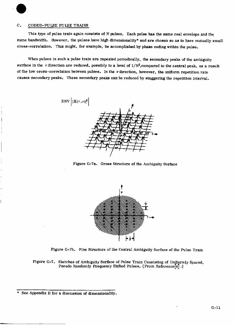
C. CODED-PULSE PULSE TRAINS

This type of pulse train again consists of N pulses. Each pulse has the same real envelope and the

same bandwidth. However, the pulses have high dimensionality* and are chosen so as to have mutually small

cross-correlation. This might, for example, be accomplished by phase coding within the pulse.

When pulses in such a pulse train are repeated periodically, the secondary peaks of the ambiguity

surface in the r direction are reduced, possibly to a level of 1/N2,compared to the central peak, as a result

of the low cross-correlation between pulses. In the _ direction, however, the uniform repetition rate

causes secondary peaks. These secondary peaks can be reduced by staggering the repetition interval.

ENV [ IX(7", v)[tt

Figure G-7a. Gross Structure of the Ambiguity Surface

Figure G-7b. Fine Structure of the Central Ambiguity Surface of the Pulse Train

Figure G-7. Sketches of Ambiguity Surface of Pulse Train Consisting of Uniformly Spaced,Pseudo Randomly Frequency Shifted Pulses. (From Reference[4] .)

* See Appendix H for a discussion of dimensionality.

G-II

D. MULTIPLE CARRIER PULSE TRAINS

The individual pulses again have the same envelope and bandwidth but different carrier frequencies.

It is assumed that the pulses in the train do not sensibly overlap in either frequency or trim and are sepa-

rated in frequency by integer multiples of a frequency differences F.

Figure G-7 shows the structure of the ambiguity surface for the case of pseudo-random shifting of the

carrier frequency of uniformly spaced pulses.

Figure G-7a illustrates the ultimate reduction of the gross structure of the secondary surfaces

possible with a properly selected pulse train. To achieve such an ambiguity surface, it is required that the

pulse train be so constructed that if it is moved in the time-frequency plane, component pulses will not co-

incide with the original positions of the pulses in more than one place at a time for any movement.

Figure G-7b shows the fine structure of the central surface. The amplitude of the secondary surfaces

can be reduced by staggering the interpulse spacing.

An examination of Figures G-5, G-6, and G-7 shows that waveform selection can be used to move the

volume of the ambiguity surface around in the T, _ plane. ' But, decreasing the volume in one region increases

it in another. This is an illustration of a general theorem that states that the volume under an ambiguity

surface is equal to unity, i.e.

CO cO

(g-21)

Figure G-5, for the uniform pulse train, illustrates this effect quite clearly.

large decrease in the volume of the central surface, compared to a single pulse, due largely to a decrease

in width in the v direction. The volume decrease results in the removed volume being shifted to many

secondary, somewhat isolated in this case, responses spread over the T, _ plane.

Repeating the pulse causes a

If the time-bandwidth product of a waveform is large, the central spike contains relatively little vol-

ume, as is illustrated bythe preceding figures. The volume, therefore, is largely contained in secondary

responses surrounding the central spike. These secondary responses can be made uniformly low by the

methods discussed. When this is done, it is conceptually and analytically convenient to have a general ap-

proximate description of the ambiguity surface. The so-called thumb tack surface, shown in Figure G-8,

provides such a description. Note that the volume in the pedestal, representing the secondary response,

is unity. This representation is especially useful when considering filter responses to several waveforms,

identical to the one to which it is matched, except shifted intime and/or frequency. It shows that the

average interference from a displaced waveform is about 1/flot o below the response of the matched wave-

form, assuming both contain the same energy.

G-12

Cross ambiguity functions X12 (T, v) describe, in general, a filter response to waveforms other than

that to which it is matched. The definition is similar to Equation (g-4), if both waveforms are normalized

to unit energy, i.e.,

O0

X12 (r, v) = f Pl (t) p_* (t - T) eJ27rvtdt (g-22)--oO

It has been shown (Reference [7])that the volume under the cross-ambiguity surface _12 (r, v)12 is also unity

This means that two large/3"o to, equal (unit) energy waveforms, having low crosscorrelation functions for

all frequency shifts, have a cross-ambiguity surfaces, _12 (T, v) 1_, representable by the pedestal only of

Figure G-8. Therefore, in general, the interference between equal energy waveforms is about 1//3 o to

below the matched waveform response.

The "thumb tack" representation assumes small average value of the t_bv (t) product, that is, _. When

for the pulse train is not small, it is not possible to realize a thumb tack surface. It is possible, however,

to construct pulse trains with small _ from pulses, not identical, which individually have large _.

Ix(r, v)12

1

1t

0

t0

Figure G-8. Thumb Tack Ambiguity Surface

G-13

To illustratethe use of ambiguity diagrams_ consider theuniformpulse train. It might be thought that

the relatively clear intervals along the r axis in Figure G-5 could be used effectively in time division multi-

plexing of pulse trains. This is true, in some cases, but for ranging from satellites, it is not attractive be-

cause, since a response can come from anywhere on approximately half the earth surface, the ambiguous

range delay is about 43 reset. This means the ambiguity surface of the pulse train can have no large

secondary peaks within 43 msee. of the central peak. Therefore, T must be greater than 43 msec. and

1/T < 23 Hz. To gain appreciable energy increase over a single pulse¢ N > 10. The half width at the

base of the central surface would then be only about 2.3 Hzo With such a narrow width, oscillator instability

and doppler frequency shifts would cause severe fading. Automatic frequency control can be used to reduce

fading; but, the long processing time makes the technique unattractive.

It is important to note that the half width of this central spike in v is the reciprocal of the pulse train

duration, NTo This is generally true for coherently processed pulse trains, forwhich the phase factor

is small.

Figure G-6 shows that repetition interval staggering reduces secondary peaks in both the r and

directions. This effect can be used to remove the restrictions on T (i. e., T > 43 msec. ). The re-

striction on the train duration, resulting from frequency instability remains, bu_ is not important because T,

and therefore the train duration, can be made small. Note that the secondary surfaces can be smeared out,

but not eliminated. The smeared surfaces introduce interference but, being at a low level, it is analogous

to noise.

G-14

APPENDIX H

RELATIONSHIP BETWEEN SYSTEM PARAMETERS

Some of the relationships between system parameters are derived in this appendix. Because the con-

cept of dimensionality of waveforms and waveform space is useful in deriving these relationships, this

section will start with a discussion of this concept. As with the use of bandwidth, time duration and phase

parameters discussedpreviously, the results obtained using the concept of dimensionality will be approxi-

mately correct. But, the accuracy of the approximation will depend on the specific problem considered.

Probably,the most straight-forwardway to illustrate the dtmensionality of a waveform space is

through the use of the sampling theorem.

Effectively this theorem states that any baseband waveform with frequency components, confined to the

interval If I < Ww Hz, can be described by amplitude samples of the waveform, separated by 1/2Ww seconds,

interpolated by appropriate sync functions. More specifically, if s(t) is a baseband waveform then

co

s(t) = E a.x sinc(2Wwt - i) (h-l)

where

, sinc x -?rx

The ai are the amplitudes of the waveform at t -- i/2Ww,where i is an integer. From a filter viewpoint,

the theorem means that any wave form,with frequency components confined to I f I < W s , can be generated

by applying appropriate amplitude samples spaced 1/2W s seconds to an ideal low pass filter with cutoff

frequency W s Hz. If the samples are spaced closer than 1/2W s second, they either cannot be picked in-

dependently, or if they are independent ,the filter will introduce correlation between samples, so that the

output will be a waveform capable of being defined by samples, separated by 1/2W s seconds.

In view of the above, if a waveform is confined to atime interval of TW

interval l f I < Ww, equation (h-l) can be written

2W 1W W

second and the frequency

s(t) = E ai sinc (2Wwt - i) (h-2)

i=1

This approximation is useful for 2W T larger than 2 or 3 and becomes better as 2W T increases. It isW W W W

possible theoretically to confine a waveform in both time and frequency, but for engineering purposes the

H-1

portion of the signal outside the time and frequency intervals can be made small enough, especially for

large 2WwT w, so that the approximation is useful.

One interpretation of equation (h-2) is that, if awaveform is confined to frequency and time intervals

of _fl <W w and Tw, it can be defined by 2WwT w or less parameters, which are the amplitudes of samples

spaced 1/2W w second. Therefore, the dimensionality of the waveform is defined as

D = 2W T (h-3)w w w

Similarly, if bandwidth of an ideal low pass channel is lfl < w s and the duration of a signal in that

channel is limited to T s, the dimensionality of the waveform space is

D = 2W T (h-4)s s s

A similar result is obtained in the case of bandpass waveforms. If s(t) is such a waveform, confined

to a bandwidth, Ww, centered at fc' i.e., its positive frequency components are restricted to the interval

W Ww <f <f + w

fc - -T c -'5-

it can be written as

s(t) = s i(t) cos w t - s (t) sin _ t (h-5)c q c

where ¢0 = 2_rfc c

s i (t) and Sq (t) are the amplitudes of the in-phase and quadrature components of the waveform and can

be independent. They arebasebandwaveforms, confinedto the frequency interval If ] < Ww/2 . From the

previous discussion of baseband waveforms,it is apparent that if s(t) is T w seconds long,both si(t) and Sq(t)

can require, at most, TwW w parameters in their description. Since they can be independent and each can

require TwW w parameters, then s (t) can require, at most, 2TwW w parameters.

Therefore, if either baseband or passband waveforms are restricted to a bandwidth Ww and a duration

T w, they can contain no more than 2TwW w independent parameters, taken here as amplitude samples. The

waveform is said to have 2TwW w dimensions,corresponding to the maximum number of independent ampli--< T andW < W , which requirestude samples. Such a waveform will fit into a waveform space,if T w s w s

the D _ D . Given the dimensionality of a waveform space,some method of defining useful waveformsw s

fitting the space is needed. The following is a discussion of one method that appears appropriate for applica-

tion to pulse train ranging and gives a useful relationship between waveform duration, bandwidth and the

number of waveforms available in the waveform space.

With Ds,the dimensionality of the waveform space, it has been shown that communication using this

space is done with the least power, if the information is coded into M symbol waveforms, M = D s + 1,

which correspond to the vertices of a regular polyhedron, with M vertices, centered at the origin of the

space. The crosscorrelation coefficient of these waveforms is - 1/D s =- 1/M - 1, corresponding geo-

metrically, to the projection of a vector from the origin to a vertex on a similar vector, drawn to any other

vertex. Figure H-1 illustrates the case where Ds = 2, M = 3. The regular polyhedron is an equilateral

H-2

Figure H-1. Waveform Space (D s = 2, M ---3)

triangle. The three vectors represent the waveforms. For baseband waveforms, the projections of a vector

on the coordinates represents the amplitude of two samples, a I and a2, from which the waveform can be

found by applying equation (h-1).

For bandpass waveforms, the projections and the coordinates represent the amplitude of simultaneous

samples of si(t) and Sq(t). Figure H-l, in this case, represents three equal amplitude, constant frequency

pulses, differing from each other only by 120 degrees in carrier phase.

In summary, this method of specifying waveforms gives, in a space of DS

M = D + 1 = 2W T + 1S S S

dimension,

with mutual crosscorrelation coefficients

M waveforms

(h-6)

1 1

D s (M - 1) (h-7)

The energy content is the same for all M waveforms. Equation (h-7) shows that the waveforms become

nearly orthogonal as D s becomes large, i.e. T -* 0 as D s increases. It should be noted that, although the

crosscorrelation coefficients are small, the autocorrelation and crosscorrelation functions of the waveforms

are not necessarily small for all time shifts. However, the correlation functions can be varied by rotation

of reference axes, and it will be assumed that usefully low values of the correlation functions can be obtained

by a suitable rotation.

Because of the role played by the phase information, detection of these waveforms must be done co-

herently, such as by a matched filter. But one important implementation of pulse train ranging utilizes

simple, amplitude modulatedpulseswhich are non-coherently detected, e.g. by envelope or square law

envelope detectors. Also, it is convenient to make these pulses of equal amplitude. In this case, since phase

information is not utilized by the detector and amplitude variations are not allowed, about the only variable

available is the time of occurrence of the pulse. If the simple pulses, at different time positions, are to have

small crosscorrelation coefficients, they must, in the bandpass case, be separated by at least 1/W s seconds.

This gives TsW s positions for the pulses in a time interval of T seconds. This will be taken as theS

H-3

number of orthogonal waveforms available in a bandpass space of D s dimensions, when simple envelope de-

tected pulses are used.

The methods discussed, for definingwaveforms and relating these to the waveform space, permit the

derivation of the relationship between bandwidth, time and address coding.

Let W c be the assigned channel bandwidth and Wu be the portion of W c usable for transmissions. If

Vst is the maximum plus and minus deviation of a transmission center frequency from the channel center

frequency, the restriction on the transmission bandwidth is

Wut = Wc - 21_stl Hz(h-8)

Vst is the sum of frequency shifts due to doppler and transmitter oscillator instability. Consequently the

transmission is confined to Wut to avoid transmission outside the assigned channel.

In addition to transmitted center frequency shifts, receiver instabilities may further restrict the

usable bandwidth. Considering the receiver instabilities only and letting Vsr be the frequency shift of the

receiver center frequency, the restriction on the usable bandwidth is

= W - 2 lVsr 1 (h-9)Wur e

Considering both possible frequency shifts, gives the maximum usable bandwidth as

Ws = Wc_ 2 (.Vstl + ,rsr,) Hz (h-10)

It is often possible to make the contribution of the receiver frequency shift to bandwidth reduction small by

receiver AFC ;thereby, making Vdt the major consideration. W s is the bandwidth limitation of the waveform

space.

The time dimension of the waveform space, T s, will usually be restricted by addressing rate require-

ments or equipment complexity. The time duration of coherently processed waveforms Tw will similarly

be restricted by equipment complexity or possibly by frequency errors. The error frequency for coherent

processing is the difference between the waveform center frequency, when applied to the matched filter, and

the filter center frequency. Temperature changes, for example, may change the filter center frequency.

If vf is the shift in filter frequency, (it may be positive or negative), an error frequency may be defined as

% = Vst- (_sr + vf) (h-ll)

As discussed in Appendix G, the matched filter response can be significantly decreased by frequency offsets

(errors). The exact relation depends upon the waveform and can be worked out from the definition of the

ambiguity function. Usually, itis desirable to limit l_el < 1/to, (where t o is the RMS waveform duration

described in Appendix B), giving abound on the coherent processing time of

t < 1 (h-12)o

Tw, which corresponds to conventional definition of waveform duration, is proportional to t o. But, the defini-

tion of t does not give a general proportionality constant. The constant can be found for any specific waveformO

H-4

from the equations of Appendix B. Consequently, .ve will place an upper bound on T w. But, the exact value has

to be worked out for a specific waveform.

To apply the concept of dimensionality and the method discussed for waveform coding to pulse trains

consider the time dimension of the waveform space divided into N intervals ,T seconds long, as shown in Fig-

ure H-2. Each T second interval contains a pulse, T w seconds long.

0 T 2T 3T (N-1)T

Figure H-2. Time Dimension of Waveform Space

The pulses, in general, are staggered aboutthe midpoints of the T second intervals and have the same

real envelope and bandwidth, but not necessarily, the same center frequency and phase function.

Let the bandwidth of the pulse train space,which is equivalent to the waveform space discussed before,

be W s and the time duration Ts, giving a dimensionality of D s = 2TsWs , as before. The pulse waveform

dimensionality is D w = 2TwWw, which must be less than or equal to the pulse space dimensionality,

= 2TW . Fromthedefinitions,T -T <-T s, W <-W andD _ D -<D . If U is the numberDp 8 w w 8 w p s

of users to be addressed, that number of distinguishable waveforms must be specified in the D s space.

This can be done by considering the pulse train as a N digit code word with one digit for each pulse space °

Each digit can take on D + 1 = M different values, which are represented by the number of nearlyP P

orthogonal waveforms (symbols) available in Dp space. If D w is less than D , frequency and/or time

shifted versions of a pulse waveform are taken as a distinct waveform, provided the frequency shift is greater

than 1/T w or that the time shift is greater than 1/W w. It is assumed that frequency and time shifts are

integral multiples of 1/T w and 1/W w, andthe allowed shifts do not take the waveform out of the pulse space.

These assumptions permit M waveforms in D space, even if D is smaller than D .p p w p

In a code word of N digits, each of which can be any one of MP

words is

U = (Mp) N

= [2TW s + 1] N

symbols, the number of different code

(h-13)

TwsThis equation relates the number of addresses, pulse train space dimensions and the number of pulses in

the train.

H-5

When N = 1, U = 2TsW s + 1. This is the case when the pulse train is coherently processed as a

whole. Itmeans-assuming 2TsW s >> 1 (which is usually true), the dimensionality of the pulse train space is

equal to the number of users. When the number of user addresses is large, this may require processing

times longer than permitted by economic or frequency stability requirements.

Increasing N and coherently processing only thepulse waveform, decreases the coherent processing

time requirements and increases the number of addresses available.

I-I-6

SECTION II

ST

Re

h

ge -

C T -

Tp -

M -

T M -

T A -

T D -

T G -

K -

77 -

C -

F T -

f -

_R -g

SECTION III.

R

N

C/N -

APPENDIX J

LIST OF SYMBOLS

Operational Parameters

time satellite spends in earth's shadow

radius of earth

satellite altitude (from center of earth)

gravitational constant of earth

traffic capacity factor

round trip propagation time

no. of messages--limit of mixing messages

message length in time

acquisition time

data gathering time

time guard band between messages

integral number of messages

data gathering technique efficiency

limit (due to time) of a modulation technique

time figure of merit for growth capacity

transmission frequency

zenith angle range error

Single Pulse Amplitude Modulation

effective bandwidth of pulse

ratio of received _ignal energy in pulse to

noise density

standard deviation of r (seconds)

number of pulses in a pulse train

carrier-to-noise ratio

J-1

SECTION IV.

E

N0

T S

W S

D S

Dp

D w -

Mp

N

m

-

-

C -

f -C

t -0

L -

q -

T

-

U -

t -op

T -

SECTION V.

Tp -

B n -

S/N -

APPENDIX J (CONT.)

LIST OF SYMBOLS

Multiple Pulse Train Ranging

energy of a pulse train

single sided noise power density

period (duration) of signal

waveform space bandwidth

dimensionality of waveform space

dimensionality of pulse space

dimensionality of pulse waveform

number of waveforms in pulse space

number of pulses in a pulse train

number of available waveforms

one-way doppler frequency shift

range rate

propagation velocity

carrier frequency

time duration of pulse train

number of simultaneous user responses

number of addresses in use at a given time

range delay measurement error

bandwidth of pulse train

number of user addresses required

coherent processing time of matched filter

period (duration) of pulse

Side Tone Modulation

mean-time-to-unlock

two-sided noise bandwidth of loop

si_aal-to-noise ratio

J-2

SECTION V.

_S/N)° -

(S/N)i -

BCL -

BTL -

T A

T C

T T

SR

Af

M

T M

T D

T G

%

C/N -

APPENDIX A.

t

O

A

R

D

APPENDIX B.

Sp(t) -

_(t) -

flo -

t -0

APPENDIX J (CONT.)

I/ST OF SYMBOI._

(CONT.) Side Tone Modulation

phase jitter

output signal-to-noiseratio

input signal-to-noiseratio

noise bandwidth of carrier loop

noise bandwidth of tone loop

acquisitiontime

carrier loop acquisitiontime

tone loop acquisitiontime

sweep rate

total frequency uncertainty

no. of messages--limit of mixing messages


data gathering time



doppler frequency shift


A Multiple Access Approach

reference (origin) time

address word

range word

data word

Waveform Descriptions and Parameters

a physical signal (function)

complex envelope


time duration of pulse train

J-3

APPENDIX B. (CONT.)

O/

(yT

M(f) -

¢ (t) -

E

NO

APPENDIX C.

% -

Bf -

R -

t t -

t -P

t D -

(S/NI v -

V -S

V -n

(S/NIp -

T D -

M -

T M -

T A -

T G -

T -P

7/ -

F T -

APPENDIX J (CONT.)

LIST OF SYMBOLS

Waveform Descriptions and Parameters

phase structure of pulse train

range delay measurement error

Fourier transform of _ (t)

phase function of _ (t)

energy of ranging waveform

white, Ganssian noise power density

FM Pulse Compression

total bandwidth of transmitted signal

bandwidth of individual filter

compression ratio

width of trigger pulse

width of transmitted pulse

time required for detection of received signal

voltage signal-to-noise ratio

signal voltage

noise voltage

output power signal-to-noise ratio (single pulse rcvr)

total detection time

no. of messagesmlimit of mixing messages


acquisition time


round trip propagation time


time figure of merit for growth capacity

J-4

APPENDIX D.

f

C

St

kI

Bf D -

Pt

C/N

p

T

fb -

fl -

f2 -

_ -

Ap _n

N -

AT -

f -S

p/2 -

f -n

% -

APPENDIX E.

N

AT

M

tCD -

Ip

lK

1 M -

LIST OF SYMBOIS (CONT.)

FM-CW Triangular Modulation

carrier frequency

rms carrier threshold

rms noise voltage per unit bandwidth

bandwidth of an FM signal

signal power at threshold


sweep period

time delay between transmitted and receivedwaveforms (round trip)

beat, or difference, frequency between transmittedand received waveforms

frequency at start of sweep

frequency at end of sweep

frequency shift due to doppler effect

measurement resolution in units of P, the sweep

period

counting resolution

range resolution interval

sweep frequency

ambignity interval

highest modulating frequency

transmitted signal bandwidth

Pseudo Random Code Technique

number of stages in shift register

time shift of code with respect to reference code

number of stages in shift register (M_N)

time for correlation decision

number of bits in a code sequence

number of bits in a code sub-sequence

number of bits in a code sub-sequence

J-5

APPE_a_IXE (CONT.)

1N

1AV -

S/N -

4_c

6T

R(_') -

R'('r) -

SR

B n

% -

K

J

(,0V

0._O

A(_) -

_d -

B(y_T) -

e(_f) -

v¢) -

s¢) -

s,¢) -

s2¢) -

A

v,¢) -

v2¢) -

Km

rl(t ) -

r2(t ) -

LIST OF SYMBOLS (CONT.)


- number of bits in a code sub-sequence

average bit length of sub-sequences

signal-to-noise ratio

phase error

time jitter

auto-correlation function

derivative of auto-correlation function

sweep rate

closed loop noise bandwidth

bandwidth of decision filter

constant

number of sub-codes in pseudo code

cut-off frequency of low pass filter

carrier frequency

a symmetric angular frequency spectrum

upper cut-off frequencymsingle sidebandr.f. spectrum

bandpass angular frequency spectrum

resultant angular frequency spectrum

modulating signal

modulated signal (carrier + modulation)

single sideband signal

double sideband (suppressed carrier) signal

carrier amplitude

modulating signal for single sideband case

modulating signal for double sideband case

local oscillator signal amplitude

recovered single sideband signal

recovered double sideband signal

J-6

APPENDIX E {CONT.)

n(t)

N0

rn(t ) -

H(_o)

O" _

n

fV

p

r d -

m° -1

d -r

o" 2 _

r

¢_ -

fro _

C -

Taeq -

h

P( ) -

p xy(j) _

S T -

S F -

RO(T ) -

s (_) -i

h(t) -

F i (_) -



- white Gaussian noise associated with r.f. signal

noise power {per unit bandwidth)

baseband noise

transfer function of receiver filter

mean square output noise power

cut-off frequency of receiver low pass filter

peak signal-to-mean square noise power ratio

round trip delay time

number of bit intervals

b_t duration or interval

variance of range error

vernier phase error

variance of vernier phase error

. propagation velocity

acquisition time

total number of correlators in receiver

relative frequency of binary sequence ( )

normalized correlation function

number of bits to be searched in time multiplex case

number of bits to be searched in frequency multi-

plex case

auto-correlation function

power spectrum, pseudo noise input signal

impulse response of an ideal filter

frequency spectrum of input pseudo noise signal

J-7

APPENDIX F.

_)

z(t)

Rxtr)

cy 2Y

s (_)x

s (_)Y

Xc¢)

x,¢)

n (t) -

S (_)n

2_B

z ¢)

S (_)z

(.0

v

PN

I_

o

F.

1

APPENDIX G.

s(t)

h(t)

A


Square Law Detection and Post Detection Filterin G

of Asymmetrical Signals

input random signal

output random signal

probability density function of the random input

probability density function of the random output

expected value of the output

autocorrelation of the output

autocorrelation of the input

variance of y (t)

power spectrum of x (t)

power spectrum of output

input carrier

input tone

input noise

noise power spectrum

bandwidth of ideal bandpass filter (rad/sec)

output of zonal filter

power spectrum of z (t)

cut-off frequency of low-pass filter

noise power out of filter

output tone-to-noise power ratio

input carrier-to-noise power ratio

ratio of F to 17o 1

Matched Filters and Ambiguity Functions

signal function

impulse response function

arbitrary time delay

J-8

APPENDIX G (CONT.)

I-'

T

E

T -O

N -

Bo -

APPENDIX H.

W w -

s(t) -

W S -

T S -

T W -

D w -

D S -

fc

M -

W C -

W -U

/_st

Vsr

vf -

Ve

t0

U

DP

N


Matched Filters and Ambiguity Functions

offset frequency

time shift

energy contained in a pulse

period of pulse train

number of pulses in a train


Relationship Between System Parameters

bandwidth of signal

baseband waveform

cutoff frequency of low-pass filter

period (duration) of signal

period of waveform

dimensionality of waveform

dimensionality of waveform space

center frequency

integer--no, of symbol waveforms

assigned channel bandwidth

portion of W useable for transmissionsc

maximum total deviation of transmission center frequency

frequency shift of receiver center frequency

shift in filter frequency

error frequency

time duration of rms waveform

no. of users to be addressed

pulse space dimensionality

no. of digits in code word (no. of pulse spaces)

J-9

3

4

5

6

7

8

9

10

11

12

13

14

15

16

17

18

19

2O

21

22

23

REFERENCES

Woodward, P.M. ; "Probability and Information Theory with Application to Radar," McGrawHill Book Company, New York.

Univac; "Autoscan, An Automatic Satellite/Computer Aid to Navigation," NASA 706,1 February 1964.

Eckler, A.R. ; "The Construction of Missile Guidance Codes Resistant to Random Interference,"BSTJ, 3.._9.9,pp. 973-994; July 1960.

Rihaczek, A.W. ; "Radar Resolution Properties of Pulse Trains," PROC. IEEE, pp. 153-164;February 1964.

Rihaczek, AoW. ; "Radar Signal Design for Target Resolution," PROC. IEEE, pp. 116-128;February 1965.

Helstrom, C.W. ; "Statistical Theory of Signal Detection," New York, Pergamon Press; 1960.

Stutt, C oA. ; "A Note on Invariant Relations for Ambiguity Functions," IRE Trans. onInformation Theory, pp. 164-167; December 1959.

Pettit, R.H. ; "Pulse Sequences with Good Autocorrelation Properties," Microwave Journal,pp. 63-67; February 1967.

Chesler, D° ; "Performance of a Multiple Address RADA System," IEEE Trans. onCommunication Tech., pp. 369-375; August 1966.

Urkowitz, H. ; "Energy Detection of Unknown Deterministic Signals," Proc. IEEE, ppo 523-531;April 1967.

Viterbi, A.M. ; "Phase Locked Dynamics in the Presence of Noise by Fokker-Planck Techniques,"Proceedings of IEEE; December 1963.

Smith, B.M. ; "A Semi-Empirical Approach to the PLL Threshold," IEEE Transactions onAerospace and Electronic Systems; July 1966.

Skolnik, M.I. ; "Introduction to Radar Systems," McGraw-Hill Book Company, Inc., 1962o

Nichols & Ranch; "Radio Telemetry," Second Edition, John Wiley and Sons, Inc., New York, 1956.

Sunde, E.D. ; "Theoretical Fundamentals of Pulse Transmission-I," B.S.T.J. 33, May 1954,pp. 579-660.

Golomb, S.W., "Deep Space Range Measurement," Research Summary No. 36-1,JPL-Pasadena, California, 15 February 1960, pp. 39-42.

Easterling, M., "Long Range Precision Ranging System," Tech. Report No. 32-80,JPL-Pasadena, California, 10 July 1961, pp. 1-7.

LeVeque, W.J., "Elementary Theory of Numbers," Theorem 3-12, po 52, Addison-Wesley,Reading, Massachusetts, 1962.

Golomb, S.W., Ed., "Digital Communication with Space Applications," Chapter 5, pp. 65-105,Prentice Hall, Englewood, New Jersey, 1964.

Plotkin, M., "Binary Sequence with Specified Minimum Distance," Trans. IRE IT-6,4 September 1954, pp. 38--49.

Zierler, N., "Linear Recurring Sequence, " J. Soc. Ind. &App. Math. 7 (1959)31-48.

Watson, E.J., "primitive Polynomials (Mod. 2), "Mathematics of Computation 16, 368-69 (1962).

Brauer, A., "On a New Class of Hadamard Determinante," Mathmatische Zeitschrift 58,219-25 (1953).

R-1

modulation techniques for range measurements from satellites

Documents

Transcript of modulation techniques for range measurements from satellites