Learning about precipitation orographic enhancement from ...

Learning about precipitation orographic enhancement fromsnow-course data improves water-balance modelingFrancesco Avanzi1, Giulia Ercolani1, Simone Gabellani1, Edoardo Cremonese2, Paolo Pogliotti2,Gianluca Filippa2, Umberto Morra di Cella2,1, Sara Ratto3, Hervè Stevenin3, Marco Cauduro4, andStefano Juglair4

1CIMA Research Foundation, Via Armando Magliotto 2, 17100 Savona, Italy2Climate Change Unit, Environmental Protection Agency of Aosta Valley, Loc. La Maladière, 48-11020 Saint-Christophe,Italy3Regione Autonoma Valle d’Aosta, Centro funzionale regionale, Via Promis 2/a, 11100 Aosta, Italy4Direzione Operativa Operations, C.V.A. S.p.A., Via Stazione 31, 11024 Châtillon, Italy

Correspondence: Francesco Avanzi ([email protected])

Abstract.

Precipitation orographic enhancement depends on both synoptic circulation and topography. Since high-elevation headwaters

are often sparsely instrumented, the magnitude and distribution of this enhancement remain poorly understood. Filling this

knowledge gap would allow a significant step ahead for hydrologic-forecasting procedures and water management in general.

Here, we hypothesized that spatially distributed, manual measurements of snow depth (courses) could provide new insights5

into this process. We leveraged 11,000+ snow-course data upstream two reservoirs in the Western European Alps (Aosta Valley,

Italy) to estimate precipitation orographic enhancement in the form of lapse rates and consequently improve predictions of a

snow-hydrologic modeling chain (Flood-PROOFS). We found that Snow Water Equivalent (SWE) above 3000 m ASL was

between 2 and 8.5 times higher than recorded cumulative seasonal precipitation below 1000 m ASL, with gradients up to 1000

mm w.e. km−1. Enhancement factors estimated by blending precipitation-gauge and snow-course data were quite consistent10

between the two hydropower headwaters (median values above 3000 m ASL between 4.1 and 4.8). Including blended gauge-

course lapse rates in an iterative precipitation-spatialization procedure allowed Flood-PROOFS to remedy underestimations of

both SWE above 3000 m ASL (up to 50%) and importantly precipitation vs. observed streamflow. Runoff coefficients based

on blended lapse rates were also more consistent from year to year that those based on precipitation gauges alone (standard

deviation of 0.06 and 0.19, respectively). Thus, snow courses bear a characteristic signature of orographic precipitation, which15

opens a window of opportunity for leveraging these data sets to improve our understanding of the mountain water budget. This

is all the more important due to their essential role in supporting water security and ecosystem services worldwide.

1

https://doi.org/10.5194/hess-2020-571Preprint. Discussion started: 26 November 2020c© Author(s) 2020. CC BY 4.0 License.

1 Introduction

Orographic precipitation is a critical driver of the Earth’s water budget (Jiang, 2003), particularly as it affects amount and20

distribution of snowpack at high elevations and thus freshwater supply and water security during the warm season (Serreze

et al., 1999; Bales et al., 2006; Viviroli et al., 2007b; Blanchet et al., 2009; Mott et al., 2014; Sarmadi et al., 2019). On shorter

time scales, orographic precipitation may contribute generating floods (Buzzi et al., 1998; Galewsky and Sobel, 2005; Panziera

et al., 2015), as well as trigger landslides and avalanches (Roe, 2005). A feature of both stratiform and convective systems

(Roe, 2005), orographic precipitation introduces sharp transitions between wet, windward and dry, leeward slopes that are25

ubiquitous across continents (rain shadows, see Houston and Hartley, 2003; Anders et al., 2006; Galewsky, 2009; Viale and

Nuñez, 2011; Da Ronco et al., 2020). These mechanisms shape local climates, ecosystems, and societies (see Michalet et al.,

2003; Roe, 2005; Poschlod, 2015, and references therein). Thus, better understanding how precipitation interacts with elevation

has important implications within and beyond Geosciences.

Orographic precipitation has already been subject of extensive research (Bonacina, 1945; Sarker, 1966; Alpert, 1986; Barros30

and Kuligowski, 1997; Smith and Barstad, 2004; Roe, 2005; Smith, 2006; Rotunno and Houze, 2007; Allamano et al., 2009;

Avanzi et al., 2015; Napoli et al., 2019; Ruelland, 2020). The emerging consensus is that distribution, intensity, and duration

of orographic precipitation depend on three modulating factors (Rotunno and Houze, 2007): synoptic-circulation patterns,

intensity of mesoscale lifting along slopes, and timing of water condensation through convection and turbulence. Interactions

across these three primary factors are notoriously elusive, with cloud microphysics, local terrain heterogeneity, and boundary-35

layer thermodynamics challenging the somewhat naive notion that precipitation increases with elevation (see Roe, 2005, for

a review). For example, Napoli et al. (2019) have showed a saturation-like effect in orographic enhancement above ∼1000

m ASL in the Alps, associated with a monotonous increase in annual-precipitation variability with elevation. This saturation

effect was also highlighted by Blanchet et al. (2009) for mean and maximum snowfall across Switzerland. Avanzi et al. (2015)

observed increased variability in extreme-precipitation quantiles with elevation and a reverse orographic effect for annual40

maximum precipitation of short duration.

This complex nature of precipitation orographic enhancement means that some of its fundamental aspects are still poorly

understood, especially across headwaters with complex terrain. This includes magnitude and seasonality of precipitation gra-

dients, how they vary across the landscape during specific events, or how they interact with temperature and relative humidity

to determine precipitation phase (Harpold et al., 2017; Avanzi et al., 2020a). These knowledge gaps are exacerbated by pre-45

cipitation measurements in snow-dominated headwaters being prone to large errors, such as wind-driven undercatch and snow

plugging (Rasmussen et al., 2012; Avanzi et al., 2014). These issues have progressively discouraged the deployment of mea-

surement stations in snow-dominated regions unless frequent maintenance and ground truthing is performed – which is very

rare due to its high costs and logistical constraints. Meanwhile, radar or satellite-based measurements in mountain terrain are

challenged by complex topography, radar-beam shielding, and ground echoing (Germann et al., 2006). Despite substantial50

efforts in recent years to achieve more reliable precipitation measurements (such as the WMO SPICE initiative, see Nitu et al.,

2018), the World’s water towers (Viviroli et al., 2007b) remain largely ungauged.

2


Better understanding precipitation distribution across mountain landscapes is not only an open question for fundamental

research, but also for operational forecasting (Frei and Isotta, 2019). Precipitation spatialization in mountain-hydrology models

is generally performed through assigning a-priori precipitation-lapse rates (e.g., see Bergström., 1992; Viviroli et al., 2007a;55

Markstrom et al., 2015) or interpolating precipitation-gauge data with various degrees of geostatistical complexity (Frei and

Schär, 1998; Daly et al., 2008; Isotta et al., 2014; Foehn et al., 2018; Frei and Isotta, 2019). While cross-validation accuracy

of these spatialization methods is high at measurement sites (e.g., mean absolute errors for monthly precipitation below ∼12

mm in Daly et al., 2008), gauge-based spatialization approaches cannot fully overcome the lack of signal at high elevations.

For instance, the seminal work by Frei and Schär (1998) considered an advanced distance-weighting scheme for spatializing60

daily precipitation across the European Alps, but the vast majority of measurement sites was located below ∼2500 m ASL.

In the US, the Parameter-elevation Relationships on Independent Slopes Model (PRISM, see Daly et al., 2008) adopts a

weighted climate–elevation relationship based on physiographic similarity, but Zhang et al. (2017) showed that this approach

underestimates both precipitation totals above ∼2400 m ASL and the seasonal precipitation lapse rate in the central Sierra

Nevada, California. It follows that predicting precipitation above this “precipitation-gauge line” at ∼2500 m ASL will always65

imply some degrees of extrapolation.

A largely unexplored solution to grasp precipitation gradients above the precipitation-gauge line is provided by snow-course

data. These are spatially distributed measurements of snow depth (HS) and optionally snow density (ρS) performed over

transects of various extent (generally 1+ km) to estimate snow-water resources across the landscape and inform water-supply

forecasting or other applications (see e.g. Hart and Gehrke, 1990; Rice and Bales, 2010). Snow-course data are routinely70

collected in various regions of the world, such as the western US (Pagano et al., 2004), Norway (Skaugen et al., 2012), or

Finland (Lundberg and Koivusalo, 2003), and have frequently been used to develop and evaluate snow-hydrologic models (Jost

et al., 2009), snow-mapping algorithms (Dressler et al., 2006; Margulis et al., 2016), or satellite-retrieval methods (Metsämäki

et al., 2005).

In the present study, we hypothesized that snow courses bear an additional, characteristic signature of seasonal orographic75

enhancement, which can be leveraged to fill the gap in precipitation measurements above the precipitation-gauge line and

improve hydrologic-model predictive skills as a result. In order to verify this hypothesis, we focused on two high-elevation,

hydropower catchments in the western European Alps (Aosta Valley, NW Italy) where 10,000+ snow-course data points have

been collected for water-supply forecasting since 2008. We combined these data with ground-based precipitation to first inves-

tigate the relationship between seasonal precipitation totals below the precipitation-gauge line and peak-accumulation snow-80

course water equivalent (SWE) above 3000 m ASL, and thus derive a climatology of lapse rates obtained by merging these

two data sets (blended lapse rates). We then leveraged these blended lapse rates to develop an iterative, two-step spatialization

procedure of precipitation that accounts for seasonal orographic effects in addition to daily precipitation variability below the

precipitation-gauge line. Third, we evaluated this spatialization procedure using streamflow measurements as well as opera-

tional snow-hydrologic modeling (S3M and Continuum, see Silvestro et al., 2013; Laiolo et al., 2014).85

3


2 Data

2.1 Study area

Aosta Valley (one of the twenty Italian administrative regions) is located at the north-western edge of the Italian peninsula

(Figure 1, a). Embraced by some of the highest peaks in the Alps (Mont Blanc, 4808 m ASL; Monte Rosa, 4634 m ASL;

and Gran Paradiso, 4061 m ASL), Aosta Valley is a typical inner-Alpine valley with marked rain shadows (Isotta et al.,90

2014). Annual precipitation totals can be as high as ∼1600-1800 mm across the south-eastern, windward slopes or the Mont-

Blanc area in the north-western corner of the region, and lower than 600 mm in the central valley. Such comparatively low

precipitation totals, coupled with pronounced temperature gradients, make this region prone to droughts and the associated

vegetation stress (Cremonese et al., 2017). Precipitation is year-round, with somewhat bimodal seasonality and prevalent peaks

in spring and fall (Crespi et al., 2018). Its topographic imbalance in precipitation distribution and the associated marked95

orographic gradients make Aosta Valley an ideal region for the present study. About 134 km2 out of 3261 km2 of Aosta Valley

are covered by glaciers (4%), meaning this is the most glacierized region in Italy (Smiraglia et al., 2015; Patro et al., 2018).

We focus on two hydropower catchments for testing our research hypothesis: Valpelline (VP) and Beauregard in Valgrisenche

(VG, see Figure 1, a and c). The total drainage area of Beauregard is ∼110 km2, 14% of which are covered by glaciers (11.4

km2); elevation ranges from ∼1800 m ASL at the outlet to ∼3500 m ASL. Valpelline spans both a larger extent and a higher100

elevation range than Beauregard; total drainage area is ∼130 km2, while minimum and maximum elevation are 1539 and 3934

m ASL, respectively. About 12.4 km2 of the drainage area of Valpelline is glacierized (9.5%). Beauregard and Valpelline are

located on two opposite sides of Aosta Valley and thus have different prevalent aspect (northwards and westwards, respectively).

Both systems are composed by a reservoir and a number of auxiliary intakes, which we lumped together as a single catchment.

Both catchments are ungauged with regard to precipitation or snow-depth automatic weather stations (Figure 1, a and c).105

2.2 Data

We employed (1) weather and snow data from the network of monitoring stations of the regional authority (https://cf.regione.

vda.it/portale_dati.php, visited on June 6, 2020), (2) reconstructed streamflow data for the two hydropower catchments of

Beauregard and Valpelline, and (3) high-elevation, manual peak-snow-depth snow courses. The study period covered water

years 2008 through 2019 based on data availability, with a specific focus on water years 2017 through 2019 when most of110

the snow-course data were collected. We define a “water year” as the period between September 1 and the following August

31, using the calendar year in which it ends (e.g., water year 2019 went from September 1 2018 to August 31 2019). We used

September to August rather than October to September (which is frequent eslewhere) because snow accumulation in this region

may start as early as September.

Weather data comprised hourly air temperature, relative humidity, incoming-shortwave-solar-radiation, wind, and total-115

precipitation data at up to∼100 (temperature),∼50 (relative humidity),∼30 (incoming shortwave solar radiation),∼60 (wind),

and ∼80 (total precipitation) measurement points. The actual number of available measurement points changed from day to

day because of potential malfunctioning or communication issues. Data were collected, processed, quality-checked, and stored

4


by the civil-protection regional authority (data access and geometry of the monitoring network: http://presidi2.regione.vda.it/

str_dataview, accessed on June 12, 2020). Quality checks were based on a mixture of automatic filtering and visual screening.120

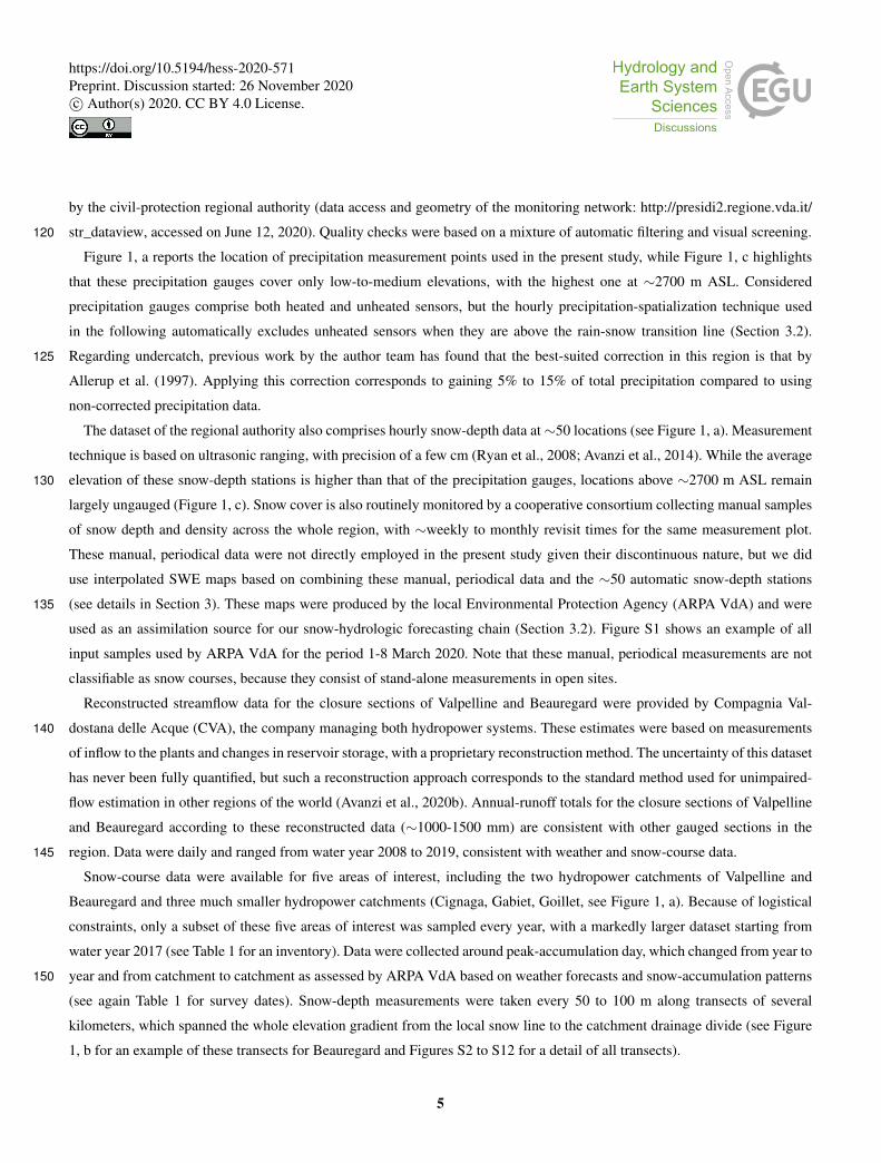
Figure 1, a reports the location of precipitation measurement points used in the present study, while Figure 1, c highlights

that these precipitation gauges cover only low-to-medium elevations, with the highest one at ∼2700 m ASL. Considered

precipitation gauges comprise both heated and unheated sensors, but the hourly precipitation-spatialization technique used

in the following automatically excludes unheated sensors when they are above the rain-snow transition line (Section 3.2).

Regarding undercatch, previous work by the author team has found that the best-suited correction in this region is that by125

Allerup et al. (1997). Applying this correction corresponds to gaining 5% to 15% of total precipitation compared to using

non-corrected precipitation data.

The dataset of the regional authority also comprises hourly snow-depth data at∼50 locations (see Figure 1, a). Measurement

technique is based on ultrasonic ranging, with precision of a few cm (Ryan et al., 2008; Avanzi et al., 2014). While the average

elevation of these snow-depth stations is higher than that of the precipitation gauges, locations above ∼2700 m ASL remain130

largely ungauged (Figure 1, c). Snow cover is also routinely monitored by a cooperative consortium collecting manual samples

of snow depth and density across the whole region, with ∼weekly to monthly revisit times for the same measurement plot.

These manual, periodical data were not directly employed in the present study given their discontinuous nature, but we did

use interpolated SWE maps based on combining these manual, periodical data and the ∼50 automatic snow-depth stations

(see details in Section 3). These maps were produced by the local Environmental Protection Agency (ARPA VdA) and were135

used as an assimilation source for our snow-hydrologic forecasting chain (Section 3.2). Figure S1 shows an example of all

input samples used by ARPA VdA for the period 1-8 March 2020. Note that these manual, periodical measurements are not

classifiable as snow courses, because they consist of stand-alone measurements in open sites.

Reconstructed streamflow data for the closure sections of Valpelline and Beauregard were provided by Compagnia Val-

dostana delle Acque (CVA), the company managing both hydropower systems. These estimates were based on measurements140

of inflow to the plants and changes in reservoir storage, with a proprietary reconstruction method. The uncertainty of this dataset

has never been fully quantified, but such a reconstruction approach corresponds to the standard method used for unimpaired-

flow estimation in other regions of the world (Avanzi et al., 2020b). Annual-runoff totals for the closure sections of Valpelline

and Beauregard according to these reconstructed data (∼1000-1500 mm) are consistent with other gauged sections in the

region. Data were daily and ranged from water year 2008 to 2019, consistent with weather and snow-course data.145

Snow-course data were available for five areas of interest, including the two hydropower catchments of Valpelline and

Beauregard and three much smaller hydropower catchments (Cignaga, Gabiet, Goillet, see Figure 1, a). Because of logistical

constraints, only a subset of these five areas of interest was sampled every year, with a markedly larger dataset starting from

water year 2017 (see Table 1 for an inventory). Data were collected around peak-accumulation day, which changed from year to

year and from catchment to catchment as assessed by ARPA VdA based on weather forecasts and snow-accumulation patterns150

(see again Table 1 for survey dates). Snow-depth measurements were taken every 50 to 100 m along transects of several

kilometers, which spanned the whole elevation gradient from the local snow line to the catchment drainage divide (see Figure

1, b for an example of these transects for Beauregard and Figures S2 to S12 for a detail of all transects).

5


Mean elevation of these snow courses was much higher than the elevation captured by the precipitation-gauge and snow-

depth-sensor networks (often above 3000 m ASL). The location of transects across each catchment was chosen to capture155

a variety of physiographic characteristics, while the number of transects for each catchment-year depended on available re-

sources. Snow depth was measured using manual probes, and location of each measurement was recorded using a portable GPS

with a precision on the order of meters. Snow-course data for each area of interest were accompanied by a few measurements

of bulk-snow density at representative locations, which were averaged to provide a reference estimate for each survey and

hence derive SWE.160

3 Methods

3.1 Estimating blended gauge-course lapse rates

We derived blended precipitation-gauge-snow-course lapse rates for Beauregard (water years 2017 through 2019) and Valpelline

(water years 2008 through 2013, 2015 through 2019) by first detecting the onset of the snow season for each catchment and

each water year as the first hour with at least 20 cm of snow on the ground for a mid-elevation, nearby snow-depth sensor165

(red squares in Figure 1, elevation was ∼1860 and 1970 m ASL for the snow depth sensor of Beauregard and Valpelline, re-

spectively). We then accumulated hourly precipitation between this onset date and the snow-course date for every precipitation

gauge in the same valley of each hydropower catchment – this was done separately for each water year. We finally derived

orographic-precipitation enhancement factors for each valley and water year by dividing seasonally cumulative precipitation

at gauges and average SWE above 3000 m ASL by seasonally cumulative precipitation at the lowest-elevation precipitation170

gauge in the same valley; these adimensional enhancement factors measure the magnitude of orographic-precipitation elevation

gradients, regardless of seasonal-precipitation totals.

Blended precipitation-gauge-snow-course lapse rates were computed as a least-square-error regression fit between elevation

and these enhancement factors. Although snow-course data were also available for other three study areas (Figure 1 and Table

1), these were too small compared to the respective valleys for deriving robust precipitation lapse rates. We therefore calibrated175

blended precipitation-gauge-snow-course lapse rates only using data from Beauregard and Valpelline (separately, see Section

3.3 for details on the use of the additional courses in this paper).

The general assumption behind blended precipitation-gauge-snow-course lapse rates is that snow-course measurements

above 3000 m ASL are representative of total precipitation fallen at those elevations from the onset of the snow season through

the snow-course date. In other words, such blended lapse rates assume that the snowpack above 3000 m ASL behaves as a180

natural precipitation gauge, with no significant mass loss throughout the accumulation season due to snowpack runoff, evapo-

ration, or sublimation. In this framework, accumulating seasonal precipitation since the first hour with at least 20 cm of snow

on the ground aimed at capturing precipitation totals for the bulk of the accumulation season, while excluding early-season

snowfall events that might result in complete or partial depletion of the snowpack.

While no continuous-time measurement of SWE was available to validate the 3000m-elevation threshold above which to185

compute average snow-course SWE, and while prescribing a constant threshold for all water years necessarily neglects inter-

6


annual variability in weather, Hantel et al. (2012) have found snow-line elevations across the Alps on the order of ∼800 m

ASL in winter and ∼3000 m ASL in summer (period 1961-2010). Thus our chosen threshold can be used to assume absence

of significant snowmelt before at least May.

Because we computed blended lapse rates using seasonally cumulative precipitation and peak SWE data, these lapse rates190

are representative of winter-precipitation gradients. Correctly capturing these seasonal gradients is vital for estimating peak

snow-cover distribution and amount and thus forecast summer water supply (e.g., see Pagano et al., 2004; Harrison and Bales,

2016), although precipitation gradients for specific storms may significantly diverge from the observed seasonal lapse rates.

Likewise, these lapse rates are not necessarily representative of summer-storm elevation gradients; in this region as well as

across the Alps in general, summer storms are mostly convection-driven (Giorgi et al., 2016), a process that is rare during195

winter and therefore cannot be fully captured by peak-season SWE measurements.

3.2 Spatialization of precipitation based on blended lapse rates

Blended precipitation-gauge-snow-course lapse rates developed in Section 3.1 were used to design an iterative, two-step

precipitation-spatialization procedure accounting for orographic effects above the precipitation-gauge line. The ultimate goal

of designing such a spatialization procedure was twofold: on the one hand, we aimed to confirm whether annual-precipitation200

totals obtained by blended precipitation-gauge-snow-course lapse rates agreed with annual reconstructed runoff, especially in

terms of annual runoff coefficients. On the other hand, we aimed to assess whether blended precipitation lapse rates could

improve hydrologic predictions (Section 3.3).

To this end, we employed the operational snow-hydrologic forecasting chain Flood-PROOFS, as validated in this region by

Laiolo et al. (2014). Flood-PROOFS consists in automatic spatialization-downscaling procedures for weather input data, a dis-205

tributed, pixel-based snow model (S3M), a distributed, pixel-based hydrologic model (Continuum), and snow-depth mapping

algorithms used for snow-data assimilation (Rebora et al., 2006; Boni et al., 2010; Laiolo et al., 2014; Silvestro et al., 2013).

In this paper, we forced Flood-PROOFS with historical data, which corresponds a standard hydrologic simulation in reanalysis

mode. The implementation of Flood-PROOFS considered in this paper runs with a spatial resolution of 120 m; the computa-

tional domain covers the entire Aosta-Valley region. More details about Flood-PROOFS’s parametrizations and spatialization210

techniques can be found in the Supporting Information, Section S1.

Similar to other snow-hydrologic models, precipitation spatialization in Flood-PROOFS relies on in-situ precipitation mea-

surements. In the current spatialization procedure, these precipitation measurements are interpolated using a modified-Kriging

approach called GRISO (Random Generator of Spatial Interpolation from uncertain Observations, see Pignone et al., 2010;

Puca et al., 2014). The most significant asset of GRISO is that interpolated precipitation for pixels including a precipitation215

gauge will maintain the same value as that measured by that precipitation gauge (in other words, measurements at precipitation-

gauge locations are preserved during interpolation). The covariance structure for each precipitation gauge is dynamical, while

precipitation-field values far from all precipitation gauges tend either towards the mean of the precipitation field observed by

gauges, or towards zero. In this paper, we chose the second option, but also set an influence radius for each precipitation gauge

7


equal to 20 km following previous validations of GRISO in Aosta Valley. No pixel of the study area was thus ”far enough”220

from all gauges for this choice to be relevant.

This one-step precipitation-spatialization procedure assumes that measurements taken by the precipitation-gauge network

are representative of the overall range of variability in precipitation across the study domain. As we outlined in the Intro-

duction and will further show in Section 4, this assumption does not necessarily hold true in mountain regions that straddle

the precipitation-gauge line, because interpolated precipitation-fields will likely underestimate precipitation totals due to oro-225

graphic effects missed by the ground-based measurement network. We overcame this issue by developing a modified, two-step

GRISO approach as follows. For each time step of interest (in our case, each hour), GRISO was first run using precipitation

gauges alone (GRISO1). Second, interpolated-precipitation values at select pixels above 2700 m ASL were enhanced according

to their elevation and the seasonal winter enhancement-factor profile calibrated in Section 3.1. Third, GRISO was re-run using

as input the measurements from the physical precipitation gauges and estimates at these select pixels (GRISO2). In this two-230

step procedure, these orographically enhanced precipitation estimates act as virtual precipitation gauges at high elevations (see

location in Figure S13), with orographic enhancement being informed by snow-course measurements at peak accumulation.

High-elevation pixels were selected by first defining a regular grid with spacing equal to 5% of the longitudinal and latitudinal

range of the study area, and then taking as candidate locations for these virtual gauges the nodes of this grid. Second, we filtered

out any candidate virtual gauge with elevation below 2700 m ASL as well as those falling outside the study area. Figure S13235

shows that the final location of these virtual precipitation gauges is coherent with the orography of out study region, and

complements the spatial coverage of the physical precipitation-gauge network (Figure 1).

3.3 Evaluating blended precipitation-gauge-snow-course lapse rates from a water-balance perspective

We evaluated precipitation estimates informed by blended precipitation-gauge-snow-course lapse rates by comparing predic-

tions of Flood-PROOFS using GRISO1 vs. those using GRISO2 (see Section 3.2). The evaluation period was water years 2017240

to 2019, since these three water years saw a peak in evaluation-data availability (particularly snow-course data). Although

water years 2017 to 2019 were also used to calibrate the blended precipitation-gauge-snow-course lapse rates and therefore

this was not a fully independent evaluation, doing so was necessary given the lack of snow-course data before 2017 for one of

the hydropower catchments (Beauregard) and the need for considering as many years as possible for lapse-rate calibration to

capture interannual variability.245

Input-data maps were first used to force the snow model of Flood-PROOFS, S3M, and generate hourly equivalent-precipitation

fields that were then used as an input for the hydrologic model Continuum; equivalent precipitation is the pixel-wise sum of

rainfall, snowpack runoff, and glacier runoff – if any (see Section S1 for details on these models). S3M can be run in two

different modes, that is, only relying on weather inputs (Open-Loop run), or assimilating SWE information from independent

sources (Full-Assim run). SWE is assimilated as both weekly maps produced by ARPA VdA through interpolation of man-250

ual measurements according to physiographic features (see Section 2.2) and daily maps produced within Flood-PROOFS by

training a multilinear regression across concurrent ultrasonic-snow-depth-sensor measurements (predictand) and physiographic

features like elevation, slope, and aspect (predictors). In the present study, evaluation of peak-SWE predictions by S3M against

8


snow courses was carried out with reference to both Open-Loop and Full-Assim simulations, to disentangle the impact of pre-

cipitation spatialization from that of data assimilation. Simulations of the complete Flood-PROOFS chain (S3M + Continuum)255

were only performed in Full-Assim mode because of computational-time constraints.

As we will show in Section 4, assimilated snow maps – and in particular those derived from snow-depth sensors – suffer

from a similar bias as that of precipitation at elevations above the snow-depth-sensor line (see Figure 1). This bias is likely

due to the snow-depth-sensor network being skewed toward representing mid-elevation snowpack. Assimilating these biased

snow maps would largely nullify the potentially positive effect of enhancing orographic effects in GRISO2, so we developed a260

correction factor by first recalibrating the snow-depth multilinear-regression model with snow-course data in addition to snow-

depth-sensor data. This recalibration was performed for each week when snow-course data were available between water years

2017 and 2019, and considering all five areas of interest were snow-course data were collected to maximize variety of data. The

mean value of the ratio between recalibrated snow-depth maps and the original ones was then used as a multiplicative factor for

original maps to remedy for high-elevation biases. This correction was only estimated for snow-depth-sensor-based maps both265

because preliminary assessments showed that they are the major source of bias compared to weekly SWE maps, and because

they are assimilated daily and as such play a much more important role than weekly SWE maps in driving Flood-PROOFS’

accuracy.

We focused on three evaluation exercises: first, we compared basinwide estimated precipitation according to GRISO1 and

GRISO2 with measured reconstructed streamflow, hence runoff coefficients; second, we ground-truthed peak-SWE predictions270

by Flood-PROOFS’s snow model (S3M) forced using GRISO1 vs. GRISO2 against snow-course data; third, we compared

cumulative daily streamflow predicted by Flood-PROOFS’s hydrologic model (Continuum) forced using GRISO1 vs. GRISO2

against reconstructed streamflow. The first and third evaluation exercises had a traditional water-balance perspective; they

determined whether estimated precipitation with and without orographic enhancement can explain annual total runoff and its

seasonal patterns (both important targets for water-supply forecasting). The second exercise assessed the impact of orographic-275

precipitation enhancement on the simulation of snow storage, an intermediate prediction target between precipitation and runoff

with significant implications beyond hydrology (e.g., avalanche forecasting, glacier mass balance).

4 Results

4.1 Water-balance climatology

Average monthly precipitation across gauges in the valleys of Beauregard and Valpelline (variable P , in mm) was bimodal,280

with peaks in November and May (Figure 2, a, reference period was water year 2009 through 2019 due to earlier gaps in P

for Beauregard, Figure S14, a). Monthly precipitation was similar between the two valleys (mean difference -2.5 ±7.1 mm).

Nonetheless, precipitation in Beauregard was up to 15 mm higher than in Valpelline during fall and winter (September to

March) and up to ∼6 mm lower during summer (April to August), which highlighted that Beauregard may be more exposed to

winter storms coming from the Mediterranean Sea, with Valpelline being more affected by summer storms from the Atlantic285

Ocean. This tallies with the bimodal and the summer-dominated precipitation regimes of the southern and northern sides of

9


the Alps, respectively (Frei and Schär, 1998; Isotta et al., 2014). However, we stress that P only accounts for precipitation

gauges, meaning precipitation totals above the precipitation-gauge line remained unaccounted. Annual P in both valleys was

consistent from year to year: ∼ 700± 84mm and ∼ 730± 94mm in Valpelline and Beauregard, respectively (Figure 3, a and

S14, a).290

According to the reference snow-depth sensors used in Section 3.1 to accumulate winter precipitation, the average snow

season started in October in both Beauregard and Valpelline (Figure 2, b, reference period is water years 2008 through 2017

due to later gaps in snow-depth data for Valpelline, see Figure 3, b). The end-of-season date generally occurred in May, with

both catchments being exposed to late snowfall events even in June. In contrast with precipitation, peak snow depth showed a

remarkable interannual variability (standard deviation of maximum annual snow depth was 31 and 77 cm at Beauregard and295

Valpelline, respectively), with three of the four water years with shallow snowpacks occurring between 2014 and 2019 (Figure

3, b and S14, b). During some of these shallow-snowpack water years, the snow cover was ephemeral at these snow-depth

sensor sites (e.g., water years 2017 at Beauregard, Figure S15, b). Monthly snow depth at the reference sensor of Valpelline

was significantly higher than that of Beauregard (Figure 2, b), which we explain because the former is at a higher elevation of

the latter (∼ 100 m).300

Reconstructed streamflow in both catchments was highly seasonal, with minimum flow during winter and maximum flow

in June, when precipitation, snow melt, and ice melt overlap (Figure 2, c, reference period is water years 2008 through 2019).

Monthly streamflow was similar between the two catchments (mean difference was -0.11 ± 18 mm), with the only exception

that streamflow in Beauregard was higher (up to ∼20 mm) between November and June and lower (up to ∼45 mm) between

July and October than in Valpelline. This is likely connected to average monthly precipitation in Beauregard being higher and305

lower than in Valpelline during winter and summer, respectively (see Figure 2, a). A second argument is favor of Beauregard

and Valpelline being hydrologically similar catchments was the similarity in precipitation-runoff relationship (Figure 3, d),

that is, the fundamental rule relating annual precipitation to annual runoff (Saft et al., 2016; Avanzi et al., 2020b). Compared

to precipitation climatology, reconstructed streamflow in both catchments showed comparatively large interannual variability

(Figure 3, c and S14, c), owing to both precipitation and climate variability.310

In summary, ground-based precipitation, streamflow, and snow-depth sensor data showed that water-supply generation in

both these two hydropower catchments is fundamentally cryosphere-dominated. They also showed that ground-based sen-

sor data located across low- and mid-elevations are largely insufficient to grasp the full water balance of these cryosphere-

dominated headwaters, as also demonstrated by (1) annual P being systematically smaller than the corresponding annual

streamflow totals (Figure 3, d), and (2) peak monthly snow depth occurring in February in both catchments. While no315

continuous-time measurement of snow-depth and SWE was available above ∼2700 m ASL (Figure 1), general consensus

in the Alps as well as our experience is that peak-SWE date occurs around April 1 or later in high-elevation, Alpine catchments

(Marty et al., 2017).

10


4.2 Precipitation vs. SWE orographic gradients

We report in Figure 4, a and b, examples of precipitation-gauge vs. snow-course orographic gradients obtained in 2018 for320

Beauregard and Valpelline, respectively. At Beauregard, precipitation gauges recorded a positive, but mild precipitation lapse

rate – on the order of ∼250 mm km−1. At Valpelline, the lapse rate recorded by precipitation gauges was even smaller, ∼75

mm km−1. The orographic trend recorded by gauges agreed with GRISO1 (see again Figure 4, a and b), which was expected

given that GRISO1 used precipitation gauges as a starting point to distribute precipitation across the landscape. Snow-course

data drew a substantially different picture from precipitation gauges, with SWE sharply increasing with elevation (Figure 4, a325

and b): ∼1000 and 567 mm w.e. km−1 in Beauregard and Valpelline, respectively. Thus, peak SWE close to (or above) 3000

m ASL in 2018 was 2-3 times total winter precipitation measured by precipitation gauges below the precipitation-gauge line.

Examining all water years for which snow-course surveys were available confirmed that these surveys yield much larger

orographic gradients than precipitation gauges in both hydropower catchments (Figure 5, a and b and Figures S15 through S25,

where missing panels imply that some of the information needed to perform this comparison was missing for that water year).330

In particular, precipitation gradients based on gauges hardly exceeded 200 mm w.e. km−1, whereas snow-course gradients were

often higher than 400 mm w.e. km−1 and reached values as high as 1000 mm w.e. km−1; snow-course-based gradients were

particularly high at Beauregard compared to Valpelline. This sharp increase in snow accumulation with elevation was consistent

across water years and was generally underestimated by both snow maps assimilated by Flood-PROOFS in proximity of the

snow-course surveys (Figure 5, a and b and S15 to S25); note that these independent maps do take into account physiography.335

This is another piece of evidence that ground-based sensor data located across low- and mid-elevations do not capture the

complete range of variability in snow distribution at high elevations.

Snow-course-based orographic gradients increased with average snow depth above 3000 m ASL (correlation coefficient ρ=

0.67, see Figure 5, c), whereas the correlation between these gradients and snow-course survey date was much weaker (ρ=

0.2, see Figure 5, d). Moreover, the correlation of snow-course orographic gradients with average snow depth above 3000 m340

ASL was statistically significant, while that with snow-course survey date was not (p-value of 0.02 and 0.52, respectively).

Thus, the choice of survey date had a limited impact on the quantification of snow-course orographic gradients, which suggests

that these gradients may preserve themselves through time.

4.3 Orographic-enhancement factors

Snow-course measurements of peak SWE above 3000 m ASL were between ∼2 and ∼8.5 times and between ∼4 and ∼5.5345

times winter cumulative precipitation at the lowest-precipitation gauge of Valpelline and Beauregard valleys, respectively

(Figure 6). Interannual variability was significant and partially driven by snowpack amount, with the four highest enhancement

factors being associated with water years with low or medium snowpack (see again Figure 6). However, this was not systematic,

since the five lowest enhancement factors were recorded during years with mixed characteristics (two with low snowpack, one

with medium snowpack, and two with high snowpack). This tallies with Figure 5, c, where only some dependency between350

snowpack amount and orographic gradients was found.

11


Contrary to snow courses, precipitation-gauge-based enhancement factors at low- and mid-elevations showed little to none

orographic trends and less interannual variability. Also, they never exceeded 2, meaning precipitation at precipitation-gauge

locations was (at best) twice that at the lowest measurement point in the same valley (Figure 6). At Valpelline, a substantial

amount of these precipitation-gauge-based enhancement factors were even lower than 1, meaning seasonal cumulative precipi-355

tation at intermediate elevations was often lower than that at the lowest-elevation gauge in the valley. This outcome is coherent

with the negative elevation trend occasionally reported in Figures S15 to S25.

Deriving a single blended lapse rate from Figure 6 was challenging, owing to the remarkable interannual variability in

enhancement factors – especially above 3000 m ASL. Several options were considered, and a first assumption was made

to exclude a indefinitely exponential growth such as that depicted by the dashed lines in Figure 6. We also assumed that360

enhancement factors larger than 6 were suspicious, and so we restricted the fitting pool to factors lower than 6. We finally

postulated a maximum value of 3 for the fitted curve, supported by an evident cluster of snow-course-based enhancement

factors from 2 to 3. While no consensus on this matter has been reached in the literature, these choices were based on scattered,

but consistent pieces of evidence showing that precipitation gradients tend to saturate at very high elevation, once the bulk of

orographic precipitation has been exhausted (e.g., see Alpert, 1986; Napoli et al., 2019). The resulting curve is depicted in red365

in Figure 6 and follows this equation:

εf = 0.395e0.628z, (1)

where εf is the predicted enhancement factor, z is elevation in km, and εf is capped to 3 where Equation 1 exceeds 3. The

95% confidence bounds for the two parameters read (0.2857, 0.5041) and (0.5223, 0.7328), respectively, with coefficient of

determination r2 = 0.44 and Root Mean Square Error (RMSE) = 0.76.370

Equation 1 was implemented in GRISO1 and used to correct predicted precipitation at virtual gauges above the precipitation-

gauge line; this spatialization procedure was then re-run to take into account orographic gradients (GRISO2, see Section 3.2).

We stress that Equation 1 only serves the scopes of this paper and is no definitive answer to the problem of capturing orographic

gradients. More work should be dedicated to fully comprehend the large scatter in enhancement factors at high elevations and

thus derive a more robust parametrization. Some starting points for future investigations are discussed in Section 5.375

Snow-depth maps produced by including snow-course data in the calibration pool allocated on average more snowpack

than those produced using only snow-depth sensors for all elevations and all water years at Beauregard (Figure 7, a to c). At

Valpelline, the map obtained by including snow courses predicted on average more snow in 2017 and 2019 and less snow in

2018 than the snow-depth-sensor-based map (Figure 7, e to g). On average across all elevations and these three water years,

the ratio between maps including snow courses and those using only snow-depth sensors was∼ 1.5 at Beauregard and∼ 2.1 at380

Valpelline, confirming a general underestimation obtained by using snow-depth sensors only. Snow-depth-sensor-based maps

were multiplied by these ratios to remedy for this bias, as explained in Section 3.3.

Note that the bias of snow-depth maps was not caused by an underestimation of snow-depth lapse rates, as it could be

expected based on results for precipitation (e.g., Figure 2). Instead, maps calibrated by including snow-course data predicted

12


steeper gradients than snow-depth sensors only in one case out of six (water year 2019 at Beauregard). This means that the385

relative underestimation of snowpack storage was often larger at the lowest elevations of the considered hydropower catchments

(that is, ∼ 2000 m ASL), and progressively smaller at higher elevations.

4.4 Evaluation of water-balance predictive accuracy

Water-year cumulative precipitation obtained using only precipitation gauges (GRISO1, variable Pv1) was consistently smaller

than observed water-year cumulative streamflow (variable Qobs) for all water years and both hydropower catchments (Figure390

8). In particular, the ratio between Qobs and Pv1 (runoff coefficient) was between 1.56 and 1.77 at Beauregard and between

1.36 and 1.81 at Valpelline (Table 2). On the contrary, runoff coefficients using GRISO2 as informed by blended precipitation-

gauge-snow-course lapse rates were between 0.78 and 0.85 at Beauregard and between 0.69 and 0.75 at Valpelline (Table 2).

This means that, in contrast to GRISO1, GRISO2 predicted more annual precipitation (variable Pv2) that streamflow in both

catchments, which is generally expected in mountain catchments where subsurface storage plays a minor role in the annual395

water balance (see Section 5). Runoff coefficients using GRISO2 were also more consistent from year to year than those based

on GRISO1 (Beauregard: standard deviation of 0.1 and 0.04 for GRISO1 and GRISO2, respectively; Valpelline: standard

deviation of 0.25 and 0.03 for GRISO1 and GRISO2, respectively). This is a further piece of evidence that GRISO2 better

captured precipitation patterns across the mountain landscape than GRISO1.

The underestimation of annual precipitation using GRISO1 was confirmed when looking at Full-Assim annual equivalent400

precipitation (Figure 8, variable Rv1 and Rv2 for GRISO1 and GRISO2, respectively); equivalent precipitation is the sum

of rainfall, snowpack-, and glacier-runoff – Section 3.3. Values of Rv1 where closer to Qobs than Pv1, with ratios between

Qobs and Rv1 between 1.03 and 1.24 at Beauregard and between 1.02 and 1.19 at Valpelline (Table 2). This confirms that

assimilating snow maps in Flood-PROOFS successfully compensated for S3M’s conceptual uncertainty in snow distribution

across the landscape (Boni et al., 2010), although some underestimation remained. Ratios betweenQobs andRv2 were, instead,405

consistently lower than 1 for all water years and both catchments (Table 2). Assimilating snow maps also reduced interannual

variability inQobs/Rv1 compared toQobs/Pv1 (standard deviation of 0.11 and 0.09 at Beauregard and Valpelline, respectively),

but Qobs/Rv2 was still much more consistent from water year to water year than Qobs/Rv1 (standard deviation of 0.04 and

0.07 at Beauregard and Valpelline, respectively).

Consistent with this general underestimation of incoming precipitation, simulated annual streamflow according to GRISO1410

(Qv1) was smaller than Qobs in four out of six catchment-water years (Qv1/Qobs between 1.23 and 1.37 in Beauregard and

between 0.95 and 1.08 in Valpelline – Table 2). Based on visual screening of observed vs. simulated cumulative hydrographs,

the unexpected overestimation of Qobs by Qv1 for two water years at Valpelline could be explained by an overestimation of

late-summer runoff, likely because of underestimated evapotranspiration or overestimated convective rainfall (Figure 8, c and

g). In all other catchment-water years, underestimation started from the beginning of the water year and thus regarded both415

winter baseflow and summer peaks (Figure 8, b, f, j, and k). Although those two water years at Valpelline with more simulated

than observed streamflow, biases of Qv1 were negative for all water years and catchments and ranged from -150 to -10 mm

(Table 2). This together with the comparatively high Root Mean Square Errors (RMSE, from ∼20 to ∼200 mm in Table 2)

13


confirmed that Flood-PROOFS simulations forced by GRISO1 generally underestimated water supply in these catchments.

Yet, Kling-Gupta Efficiencies (KGE, see Gupta et al., 2009; Kling et al., 2012) for Qv1 were consistently higher than 0.65 and420

thus well above the benchmark represented by mean flow (-0.41, see Knoben et al., 2019), which has been often regarded as an

arguable threshold between ”bad” and ”good” model performance (Schaefli and Gupta, 2007; Knoben et al., 2019). Contrary

to RMSE and biases, KGE is the composition of bias, variability, shape, and timing error terms (Santos et al., 2018), meaning

the issue with GRISO1-based simulations was really with total volume rather than with seasonal patterns.

Simulations using GRISO2 improved Qv2/Qobs compared to Qv1/Qobs for four out of six catchment-water years (Table 2425

and Figure 8). Predictions ofQv2 also yielded smaller biases and RMSEs (as absolute values) for all water years and catchments

(Table 2). The improvement of Qv2 over Qv1 was particularly evident during the late-melt period (that is, from May on), when

the highest elevations in these catchments start contributing runoff (Figure 8). Improvements during the accumulation period

were much more modest, likely because streamflow generation during that period of the year is governed by processes that we

did not focus on here (e.g., groundwater flow, year-round glacier runoff due to basal melt). KGE coefficients also improved in430

five out of six catchment-water years, reaching values as high as 0.93.

Focusing on SWE, simulations of S3M using GRISO1 underestimated snow-course measurements both whether an Open-

Loop and whether a Full-Assim mode was used (Figure 9). This underestimation was particularly significant for Open-Loop

simulations, which agreed with results for precipitation vs. equivalent precipitation above (Table 2), whereas it showed no con-

sistent trend with elevation, which is instead consistent with results in Section 4.3 and Figure 7 regarding snowpack elevation435

gradients being particularly elusive to capture. Biases using GRISO2 were smaller than those using GRISO1 in five out of six

catchment-water years (Full Assim mode), but again elevation trends were inconsistent (Figure 9). Using an Open-Loop simu-

lations with GRISO2 would actually overestimate at the highest elevations in two out of six cases (2017 and 2018, Valpelline,

Figure 9, d and h).

We derived two main results from this final focus on SWE: the first is an expected, net improvement in predicting high-440

elevation SWE when snow-course measurements are used in model development (especially at Beauregard). The second is

that precipitation orographic gradients are highly seasonal as well as spatially variable, and remain challenging to fully capture

with a one-fits-all approach as the one we used here (e.g., Equation 1 and Figure 7, d and h).

5 Discussion

5.1 Main findings445

Snow courses have been a frequent option for conducting snow surveys since the seminal 1910 campaign by Church (1914,

1933) at Mount Rose, Nevada (US). Compared to stand-alone devices like snow pillows (Cox et al., 1978), courses allow

operators to capture spatial variability of snow cover and so derive a more representative estimate of SWE across the landscape

(Malek et al., 2017). This is why courses are now a cornerstone of water-supply forecasting in the western US (Pagano et al.,

2004; Harrison and Bales, 2016) and elsewhere (Metsämäki et al., 2005). In addition to their century-old role as indicator of450

snow water resources, in this paper we hypothesized that snow courses could be rethought as natural precipitation gauges,

14


in the hope that they could provide new information about precipitation totals and their orographic trends at elevations that

are usually ungauged. This hypothesis follows intuitions by other authors, such as Lundquist et al. (2015) or Zhang et al.

(2017), who used pillow SWE and snow depth as a surrogate of precipitation, respectively. Others, such as Immerzeel et al.

(2015), addressed this problem by inferring precipitation from glacier mass balances and runoff. Our novelty was to mine new455

information from snow courses, which provide spatial snapshots in lieu of point values.

The main findings of this paper in this regard are two. First, peak-season snow-course SWE above 3000 m ASL can be 2 to

8.5 times higher than measured winter cumulative precipitation at elevations below 2000 m ASL (Figure 6), with orographic

trends that are up to five times those captured by the precipitation-gauge network (Figure 2). While orographic precipitation has

been a target of extensive research so far (see the Introduction), extrapolating precipitation-gauge signal above the precipitation-460

gauge line still lacks solid guidelines (Ruelland, 2020). In this paper, we contributed highly-needed, multi-year estimates of

orographic trends across sharp altitudinal gradients.

Second, leveraging snow courses to refine the precipitation- and snow-depth-spatialization algorithms of an operational

flood-forecasting chain (Flood-PROOFS) allowed for improvements in modeling accuracy not only for SWE (Figure 9), but

importantly for the whole water balance (Figure 8). This result is encouraging given that no model recalibration was performed,465

and as such we did not mix the effect of precipitation correction with other confounding factors that may lead to equifinality

issues (Beven and Freer, 2001; Lundquist et al., 2015). Although the bulk of mountain river basins in the European Alps lies

below 2000 m ASL (Elsen et al., 2020), areas above the precipitation-gauge line are a fundamental hydropower resource and

represent a significant portion of higher-elevation mountain ranges such as the Himalayas. This paper outlined opportunities to

obtain more robust hydrologic predictions without necessarily investing into long recalibration efforts.470

Despite these promising findings, the question remains whether our blending approach (Section 3.1) reconstructed the true

precipitation lapse rate, or whether it captured other drivers of snowpack distribution at high elevations (e.g., wind drift). While

both scenarios would be an argument in favor of using snow courses for informing hydrologic predictions, only the first would

imply that we achieved the right answer for the right reason (Kirchner, 2006). In essence, this question points to determining

whether snow-course data are primarily a reflection of orographic precipitation or, e.g., of wind drift or solar radiation.475

Several hints point to our reconstruction method capturing actual orographic trends in precipitation, rather than other snow-

distribution processes. First, previous studies in the Alps already showed that annual mean precipitation at 1000-2000 m

ASL is generally up to 2 times precipitation below 1000 m ASL, (Frei and Schär, 1998; Napoli et al., 2019), a mechanism

that the precipitation network at Beauregard and Valpelline did not fully capture but that is consistent with our estimates of

blended orographic-enhancement factors (Figure 6 and Equation 1). Second, several previous attempts to improve estimates of480

hydrologic models in mountain regions through snow-data assimilation alone reported inconclusive results (Tang and Letten-

maier, 2010), whereas the clear improvements in this study suggest that we did capture at last some components of orographic

precipitation in addition to snow patterns. Third, we computed orographic-enhancement factors by averaging snow-course

measurements above 3000 m ASL rather than considering each of them individually, in an effort to reduce the effects of small-

scale spatial variability. Fourth, values of snow-course SWE at elevations close to the local precipitation-gauge line (∼2000 m485

ASL) are comparable to cumulative precipitation estimated by the nearest gauge (Figure 4), which suggests that the connection

15


between precipitation-gauge-based and snow-course-based lapse rates was smooth and realistic. Thus, we conclude that snow

courses do bear a characteristic signature of precipitation orographic enhancement.

5.2 Implications

The fact that snow courses reflect orographic gradients has three main implications. First, it shows that the lack of measurements490

above the precipitation-gauge line plays an important role in the misrepresentation of orographic gradients. Many previous

papers have already reported that precipitation-gauge networks tend to underestimate precipitation at high elevations, including

Zhang et al. (2017) in the Sierra Nevada of California or Ruelland (2020) in the French Alps, among others. However, this

misrepresentation has often been explained in combination with undercatch (Valery et al., 2009; Zhang et al., 2017; Collados-

Lara et al., 2018), rather than as a peculiar effect of precipitation undersampling at high elevations (Lundquist et al., 2015;495

Ruelland, 2020). In fact, the magnitude of orographic enhancement inferred through snow courses (Figure 6) was certainly

larger than what could be estimated based on standard correction approaches for undercatch (see Rasmussen et al., 2012;

Kochendorfer et al., 2017, and Section 2.2). Also, both GRISO1 and snow-depth-sensor-based maps underestimated these

orographic gradients: we conclude that the main cause of this misrepresentation was the lack of data above the precipitation-

gauge line. Even though measuring precipitation across cryosphere-dominated headwaters is no easy task (Rasmussen et al.,500

2012), this paper shows that this is still an urgent priority for future research.

Second, snow courses emerge as a valuable source of information not only to estimate snow water resources, but more

generally precipitation distribution. This role of snow courses has been at the foundation of their use as predictors of annual

runoff in water-supply forecasting (Hart and Gehrke, 1990; Pagano et al., 2004), but in that context snow courses are used in

a lumped way and their orographic signature is never fully leveraged. More in general, the value of snow courses has often505

been overlooked in favor of temporally more dense, but also much less spatially diverse automatic devices like snow pillows or

snow-depth sensors. The result is that snow courses, or other labor-intensive survey methods, are a rare feature of operational

snow surveys, when they have not been discontinued already (see the case of The Historical Snow Survey of Great Britain in

Spencer et al., 2014). The significant variability in enhancement factors between Beauregard and Valpelline, along with the fact

that snow-course-based enhancement factors were significantly larger than those based on precipitation gauges, demonstrates510

that collecting spatially distributed snow data is still worth the effort. Moreover, the longest snow-course time-series will

soon approach one century (Huning and AghaKouchak, 2020), meaning these courses could be used to explore orographic

enhancement from a climatological standpoint. Recent advances in remote sensing, such as the Airborne Snow Observatory

(Painter et al., 2016) or the Sentinel-1-based snow-depth retrieval algorithm by Lievens et al. (2019), could also be considered

as less time-consuming alternatives, with only a minor drop in accuracy – if any.515

Third, correctly capturing orographic gradients matters, despite this component being often simplified in many hydrologic

models (see Ruelland, 2020, and the Introduction). More specifically, our results quantified that only relying on low- to mid-

elevation precipitation gauges may lead to underestimating both headwater snowpack (Figure 9) and annual runoff (Table

2) by up to 50% or more. This agrees with Lundquist et al. (2015), who also found errors of 50% or more with respect to

high-elevation snow pillows for specific storms as represented by gridded precipitation datasets that only used low-elevation520

16


precipitation data. Also, our results suggest that snow (and consequently runoff) predictions benefit from a multi-source frame-

work, where both precipitation-spatialization and snow-assimilation protocols are involved (see again Figure 9).

5.3 Sources of uncertainty and outlook

We made a number of assumptions that may have represented sources of potential uncertainty and thus opportunities for future

work. First, we primarily focused on elevation gradients, since these are the most important factors driving the mountain water525

budget (Bales et al., 2006). Doing so was at the expenses of exploring other spatial patterns, such as those driven by aspect

and slope. The variability in enhancement factors between the predominantly north-facing Beauregard and the south-to-west

facing Valpelline suggests that these additional factors are important. Our results also showed significant interannual variability

in enhancement factors, which somehow disagrees with the recurring finding that snow patterns are consistent from year to

year (Zheng et al., 2018). Future work could focus on deriving a multivariate alternative to Equation 1 that fully embraced530

physiographic features besides elevation, and in particular aspect, slope, and canopy cover (Malek et al., 2017). For example,

Vögeli et al. (2016) showed significant improvements for a spatially distributed snow model when scaling its predictions with

remote-sensing data. Winter climatology may also be considered as an additional predictor of orographic enhancement, for

example in the form of predominant synoptic conditions as done by Garavaglia et al. (2010).

Second, we applied GRISO2 across the whole water year (September to August), although we estimated our orographic-535

enhancement factors only with winter data. This was done both for consistency reasons, and because we expect orographic

enhancement to be at play during summer too. Nonetheless, mechanisms behind summer precipitation are significantly different

from those behind winter precipitation (convective vs. stratiform, see e.g. Avanzi et al., 2015). No specific dataset can replace

our snow courses during summer, but at the same time efficiency of precipitation gauges is much higher for rainfall than

snowfall (Peck, 1972). Thus, measuring precipitation at elevations above 3000 m ASL is much more feasible during summer540

than winter, which could be leveraged in the future to explore specific parametrizations of Equation 1 for summer.

Third, we converted snow-course snow depth to SWE using one average density value for each catchment-water year, with

density being measured to a significantly smaller number of locations than snow depth due to logistical constraints. We expect

this assumption to play a minor role in our assessment, given that snow-density spatial variability is much smaller than that of

snow depth (López Moreno et al., 2013). Yet, Raleigh and Small (2017) showed that snow-density modeling becomes the major545

source of uncertainty when mapping basin-wide SWE with Lidar. This means that targeted campaigns measuring snow-density

variability across the landscape would still be beneficial to improve this work.

Fourth, peak-SWE date was assessed based on expert knowledge and changed from year to year. This protocol was different

from other snow-course surveys, which are generally performed on recurring dates every year (Hart and Gehrke, 1990). Based

on results in Figure 5, we expect this assumption to have little to no impact on our estimates of orographic gradients. On550

the other hand, changing survey date based on when peak-SWE is supposed to occur favored our work because it allowed

us to assume that snow-course SWE represented total winter precipitation falling at that location. Doing so would have been

challenging with monthly courses performed on pre-defined dates.

17


Fifth, our assessment in Figure 8 assumed that the subsurface storage was a secondary source of annual streamflow compared

to precipitation, so that Q/P < 1 rather than Q/P > 1 was the desired outcome. We are lacking the necessary data to fully555

resolve the water budget of these catchments, as done in California by Avanzi et al. (2020b). Still, the interannual consistency

in Q/P based on GRISO2, together with the quasi linearity in precipitation-runoff relationship (Figure 3), do suggest a clear

correspondence between annual precipitation and annual runoff, and thus that Q/P > 1 by GRISO1 was suspicious.

Sixth, we did not use any additional precipitation dataset in addition to precipitation gauges (for example, radars). Besides

known issues with radars in mountain regions (see the Introduction), this was also because the present study leveraged the560

precipitation-spatialization algorithm that is currently being maintained by the author team in Aosta Valley (Laiolo et al., 2014).

Future efforts by this team include an operational deployment of GRISO2 for flood forecasting, potentially in combination with

a newly developed, in-house precipitation product based on conditional merging between precipitation gauges and radar.

6 Conclusions

We addressed the recurring challenge of estimating precipitation across ungauged, high-elevation headwaters above the “precipitation-565

gauge line”. We did so by hypothesizing that snow courses could be rethought as natural precipitation gauges and thus be

leveraged to reconstruct blended precipitation-gauge-snow-course lapse rates. We found that winter precipitation estimated

through peak-SWE snow-course data was 2 to 8.5 times higher than what recorded by nearby precipitation gauges, evidence

that orographic precipitation in this inner Alpine valley develops with unexpectedly large orographic gradients that would be

missed by using low-to-mid-elevation precipitation gauges. These gradients were also miscaptured by snow-depth sensors,570

both because their elevation range is only slightly larger than that of precipitation gauges and because they are installed in open

and flat areas. Elevation trends of snow-course data were highly seasonal, with only some correlation with mean seasonal snow

depth; this revealed a feedback mechanism between orographic enhancement and winter precipitation climatology that par-

tially challenged the generalization of our results. Blending precipitation-gauge and snow-course data into a unique lapse rate

and using this information in an operational hydrologic-modeling chain (Flood-PROOFS) allowed us to improve predictions575

for not just Snow Water Equivalent, but importantly for the water budget (specifically, the interannual consistency of runoff

coefficients). Snow courses bear a signature of orographic enhancement, which we successfully mined to gain insight into the

process of orographic precipitation and improve real-world hydrologic models.

Code and data availability. Sources of data used in this are reported in Section 2.2, and comprise the Aosta Valley Regional Authority

(https://cf.regione.vda.it/portale_dati.php, visited on July 30, 2020), Compagnia Valdostana delle Acque (https://www.cvaspa.it/_welcome_/,580

visited on July 30, 2020), and the Aosta Valley Environmental Protection Agency (http://www.arpa.vda.it/it/, visited on July 30, 2020). Flood-

PROOFS is described in Laiolo et al. (2014) and partially available at https://github.com/c-hydro (visited on July 30, 2020).

18


Author contributions. FA, GE, and SG conceived the investigation, with contributions from all coauthors. FA and GE carried out analyses

and performed model simulations. EC, PP, GF, and UMdC collected snow-course data and prepared SWE maps, as well as shared general

knowledge about cryospheric processes in the study catchments. SR and HS provided weather and snow data collected by the Aosta Valley585

Regional Authority, as well as shared general knowledge about hydrologic processes in the study catchments. MC and SJ provided recon-

structed streamflow data and shared general knowledge about hydropower processes in the study catchments. FA, GE, SG, and EC led result

interpretations, with inputs from all coauthors. FA prepared the manuscript, with inputs from all coauthors.

Competing interests. Authors declare no competing interest.

Acknowledgements. This work was supported by the Aosta Valley Regional Administration and CVA S.p.A.590

19


References

Allamano, P., Claps, P., Laio, F., and Thea, C.: A data-based assesment of the dependence of short-duration precipitation on elevation, Physics

and Chemistry of the Earth, 34, 635–641, https://doi.org/10.1016/j.pce.2009.01.001, 2009.

Allerup, P., Madsen, H., and Vejen, F.: A Comprehensive Model for Correcting Point Precipitation, Hydrology Research, 28, 1–20,

https://doi.org/10.2166/nh.1997.0001, https://doi.org/10.2166/nh.1997.0001, 1997.595

Alpert, P.: Mesoscale indexing of the distribution of orographic precipitation over high mountains, Journal of Climate and Applied Meteo-

rology, 25, 532–545, https://doi.org/http://dx.doi.org/10.1175/1520-0450(1986)025<0532:MIOTDO>2.0.CO;2, 1986.

Anders, A. M., Roe, G. H., Hallet, B., Montgomery, D. R., Finnegan, N. J., and Putkonen, J.: Spatial patterns of precipitation and topography

in the Himalaya, in: Tectonics, Climate, and Landscape Evolution, Geological Society of America, https://doi.org/10.1130/2006.2398(03),

https://doi.org/10.1130/2006.2398(03), 2006.600

Avanzi, F., De Michele, C., Ghezzi, A., Jommi, C., and Pepe, M.: A processing-modeling routine to use SNOTEL hourly data in snowpack

dynamic models, Advances in Water Resources, 73, 16–29, https://doi.org/10.1016/j.advwatres.2014.06.011, 2014.

Avanzi, F., De Michele, C., Gabriele, S., Ghezzi, A., and Rosso, R.: Orographic Signature on Extreme Precipitation of Short Durations,

Journal of Hydrometeorology, 16, 278–294, https://doi.org/10.1175/JHM-D-14-0063.1, 2015.

Avanzi, F., Maurer, T., Glaser, S. D., Bales, R. C., and Conklin, M. H.: Information content of spatially distributed ground-based605

measurements for hydrologic-parameter calibration in mixed rain-snow mountain headwaters, Journal of Hydrology, 582, 124 478,

https://doi.org/https://doi.org/10.1016/j.jhydrol.2019.124478, 2020a.

Avanzi, F., Rungee, J., Maurer, T., Bales, R., Ma, Q., Glaser, S., and Conklin, M.: Climate elasticity of evapotranspiration shifts

the water balance of Mediterranean climates during multi-year droughts, Hydrology and Earth System Sciences, 24, 4317–4337,

https://doi.org/10.5194/hess-24-4317-2020, https://hess.copernicus.org/articles/24/4317/2020/, 2020b.610

Bales, R., Molotch, N. P., Painter, T. H., Dettinger, M. D., Rice, R., and Dozier, J.: Mountain hydrology of the western United States, Water

Resources Research, 42, W08 432, https://doi.org/10.1029/2005WR004387, 2006.

Barros, A. P. and Kuligowski, R. J.: Orographic effects during a severe wintertime rainstorm in the Appalachian mountains, Monthly Weather

Review, 126, 2648–2672, https://doi.org/http://dx.doi.org/10.1175/1520-0493(1998)126<2648:OEDASW>2.0.CO;2, 1997.

Bergström., S.: The HBV model - its structure and applications., Tech. rep., SMHI Reports Hydrology, 1992.615

Beven, K. and Freer, J.: Equifinality, data assimilation, and uncertainty estimation in mechanistic modelling of complex environmental

systems using the GLUE methodology, Journal of Hydrology, 249, 11 – 29, https://doi.org/https://doi.org/10.1016/S0022-1694(01)00421-

8, 2001.

Blanchet, J., Marty, C., and Lehning, M.: Extreme value statistics of snowfall in the Swiss Alpine region, Water Resources Research, 45,

W05 424, https://doi.org/10.1029/2009WR007916, 2009.620

Bonacina, L. C. W.: Orographic rainfall and its place in the hydrology of the globe, Quarterly Journal of the Royal Meteorological Society,

71, 41–55, https://doi.org/10.1002/qj.49707130705, 1945.

Boni, G., Castelli, F., Gabellani, S., Machiavello, G., and Rudari, R.: Assimilation of MODIS snow cover and real time snow depth point

data in a snow dynamic model, in: 2010 IEEE International Geoscience and Remote Sensing Symposium, pp. 1788–1791, 2010.

Buzzi, A., Tartaglione, N., and Malguzzi, P.: Numerical Simulations of the 1994 Piedmont Flood: Role of Orography and Moist Processes,625

Monthly Weather Review, 126, 2369–2383, https://doi.org/http://dx.doi.org/10.1175/1520-0493(1998)126<2369:NSOTPF>2.0.CO;2,

1998.

20


Church, J. E.: Recent studies of snow in the United States, Quarterly Journal of the Royal Meteorological Society, 40, 43–52,

https://doi.org/10.1002/qj.49704016905, https://rmets.onlinelibrary.wiley.com/doi/abs/10.1002/qj.49704016905, 1914.

Church, J. E.: Snow Surveying: Its Principles and Possibilities, Geographical Review, 23, 529 – 563, 1933.630

Collados-Lara, A.-J., Pardo-Igúzquiza, E., Pulido-Velazquez, D., and Jiménez-Sánchez, J.: Precipitation fields in an alpine Mediterranean

catchment: Inversion of precipitation gradient with elevation or undercatch of snowfall?, International Journal of Climatology, 38, 3565–

3578, https://doi.org/10.1002/joc.5517, https://rmets.onlinelibrary.wiley.com/doi/abs/10.1002/joc.5517, 2018.

Cox, L., Bartee, L., Crook, A., Farnes, P., and Smith, J.: The care and feeding of snow pillows, in: Proceedings of the 46th Annual Western

Snow Conference, pp. 40–47, Otter Rock, Oregon, 1978.635

Cremonese, E., Filippa, G., Galvagno, M., Siniscalco, C., Oddi, L., Morra di Cella, U., and Migliavacca, M.: Heat wave hinders green

wave: The impact of climate extreme on the phenology of a mountain grassland, Agricultural and Forest Meteorology, 247, 320 – 330,

https://doi.org/https://doi.org/10.1016/j.agrformet.2017.08.016, 2017.

Crespi, A., Brunetti, M., Lentini, G., and Maugeri, M.: 1961–1990 high-resolution monthly precipitation climatologies for Italy, International

Journal of Climatology, 38, 878–895, https://doi.org/10.1002/joc.5217, https://rmets.onlinelibrary.wiley.com/doi/abs/10.1002/joc.5217,640

2018.

Da Ronco, P., Avanzi, F., De Michele, C., Notarnicola, C., and Schaefli, B.: Comparing MODIS snow products Col-

lection 5 with Collection 6 over Italian Central Apennines, International Journal of Remote Sensing, 41, 4174–4205,

https://doi.org/10.1080/01431161.2020.1714778, 2020.

Daly, C., Halbleib, M., Smith, J. I., Gibson, W. P., Doggett, M. K., Taylor, G. H., Curtis, J., and Pasteris, P. P.: Physiographically sensitive645

mapping of climatological temperature and precipitation across the conterminous United States, International Journal of Climatology, 28,

2031–2064, https://doi.org/10.1002/joc.1688, 2008.

Dressler, K. A., Leavesley, G. H., Bales, R. C., and Fassnacht, S. R.: Evaluation of gridded snow water equivalent and satellite snow cover

products for mountain basins in a hydrologic model, Hydrological Processes, 20, 673–688, https://doi.org/10.1002/hyp.6130, 2006.

Elsen, P. R., Monahan, W. B., and Merenlender, A. M.: Topography and human pressure in mountain ranges alter expected species responses650

to climate change, Nature Communications, 11, 1–10, 2020.

Foehn, A., Hernández, J. G., Schaefli, B., and Cesare, G. D.: Spatial interpolation of precipitation from multiple rain gauge net-

works and weather radar data for operational applications in Alpine catchments, Journal of Hydrology, 563, 1092 – 1110,

https://doi.org/https://doi.org/10.1016/j.jhydrol.2018.05.027, 2018.

Frei, C. and Isotta, F. A.: Ensemble Spatial Precipitation Analysis From Rain Gauge Data: Methodology and Application in the European655

Alps, Journal of Geophysical Research: Atmospheres, 124, 5757–5778, https://doi.org/10.1029/2018JD030004, 2019.

Frei, C. and Schär, C.: A precipitation climatology of the Alps from high-resolution rain-gauge observations, International Journal of Clima-

tology, 18, 873–900, https://doi.org/10.1002/(SICI)1097-0088(19980630)18:8<873::AID-JOC255>3.0.CO;2-9, 1998.

Galewsky, J.: Rain shadow development during the growth of mountain ranges: An atmospheric dynamics perspective, Journal of Geo-

physical Research: Earth Surface, 114, https://doi.org/10.1029/2008JF001085, https://agupubs.onlinelibrary.wiley.com/doi/abs/10.1029/660

2008JF001085, 2009.

Galewsky, J. and Sobel, A.: Moist Dynamics and Orographic Precipitation in Northern and Central California during the New Year’s Flood

of 1997, Monthly Weather Review, 133, 1594–1612, https://doi.org/10.1175/MWR2943.1, https://doi.org/10.1175/MWR2943.1, 2005.

21


Garavaglia, F., Gailhard, J., Paquet, E., Lang, M., Garçon, R., and Bernardara, P.: Introducing a rainfall compound distribution model based

on weather patterns sub-sampling, Hydrology and Earth System Sciences, 14, 951–964, https://doi.org/10.5194/hess-14-951-2010, https:665

//hess.copernicus.org/articles/14/951/2010/, 2010.

Germann, U., Galli, G., Boscacci, M., and Bolliger, M.: Radar precipitation measurement in a mountainous region, Quarterly Journal of the

Royal Meteorological Society, 132, 1669–1692, https://doi.org/10.1256/qj.05.190, 2006.

Giorgi, F., Torma, C., Coppola, E., Ban, N., Schär, C., and Somot, S.: Enhanced summer convective rainfall at Alpine high elevations in

response to climate warming, Nature Geoscience, 9, 584–589, 2016.670

Gupta, H. V., Kling, H., Yilmaz, K. K., and Martinez, G. F.: Decomposition of the mean squared error and NSE performance criteria: Impli-

cations for improving hydrological modelling, Journal of Hydrology, 377, 80–91, https://doi.org/10.1016/j.jhydrol.2009.08.003, 2009.

Hantel, M., Maurer, C., and Mayer, D.: The snowline climate of the Alps 1961–2010, Theoretical and applied climatology, 110, 517–537,

2012.

Harpold, A. A., Kaplan, M. L., Klos, P. Z., Link, T., McNamara, J. P., Rajagopal, S., Schumer, R., and Steele, C. M.: Rain or snow: hydrologic675

processes, observations,prediction, and research needs, Hydrology and Earth System Sciences, 21, 1–22, https://doi.org/10.5194/hess-21-

1-2017, https://www.hydrol-earth-syst-sci.net/21/1/2017/, 2017.

Harrison, B. and Bales, R.: Skill Assessment of Water Supply Forecasts for Western Sierra Nevada Watersheds, Journal of Hydrologic

Engineering, 21, 04016 002, https://doi.org/10.1061/(ASCE)HE.1943-5584.0001327, 2016.

Hart, D. and Gehrke, F.: Status of the California cooperative snow survey program, in: Proceedings of the 58th Annual Western Snow680

Conference, pp. 9–14, Sacramento, California, 1990.

Houston, J. and Hartley, A. J.: The central Andean west-slope rainshadow and its potential contribution to the origin of hyper-aridity in the

Atacama Desert, International Journal of Climatology, 23, 1453–1464, https://doi.org/10.1002/joc.938, https://rmets.onlinelibrary.wiley.

com/doi/abs/10.1002/joc.938, 2003.

Huning, L. S. and AghaKouchak, A.: Approaching 80 years of snow water equivalent information by merging different data streams, Scien-685

tific Data, 7, 1–11, 2020.

Immerzeel, W. W., Wanders, N., Lutz, A. F., Shea, J. M., and Bierkens, M. F. P.: Reconciling high-altitude precipitation in the upper Indus

basin with glacier mass balances and runoff, Hydrology and Earth System Sciences, 19, 4673–4687, https://doi.org/10.5194/hess-19-4673-

2015, https://hess.copernicus.org/articles/19/4673/2015/, 2015.

Isotta, F. A., Frei, C., Weilguni, V., Percec Tadic, M., Lassègues, P., Rudolf, B., Pavan, V., Cacciamani, C., Antolini, G., Ratto, S. M., Munari,690

M., Micheletti, S., Bonati, V., Lussana, C., Ronchi, C., Panettieri, E., Marigo, G., and Vertacnik, G.: The climate of daily precipitation in the

Alps: development and analysis of a high-resolution grid dataset from pan-Alpine rain-gauge data, International Journal of Climatology,

34, 1657–1675, https://doi.org/10.1002/joc.3794, 2014.

Jiang, Q.: Moist dynamics and orographic precipitation, Tellus A, 55, 301–316, https://doi.org/10.1034/j.1600-0870.2003.00025.x, https:

//onlinelibrary.wiley.com/doi/abs/10.1034/j.1600-0870.2003.00025.x, 2003.695

Jost, G., Dan Moore, R., Weiler, M., Gluns, D. R., and Alila, Y.: Use of distributed snow measurements to test and

improve a snowmelt model for predicting the effect of forest clear-cutting, Journal of Hydrology, 376, 94 – 106,

https://doi.org/https://doi.org/10.1016/j.jhydrol.2009.07.017, 2009.

Kirchner, J. W.: Getting the right answers for the right reasons: Linking measurements, analyses, and models to advance the science of

hydrology, Water Resources Research, 42, https://doi.org/10.1029/2005WR004362, 2006.700

22


Kling, H., Fuchs, M., and Paulin, M.: Runoff conditions in the upper Danube basin under an ensemble of climate change scenarios, Journal

of Hydrology, 424-425, 264 – 277, https://doi.org/https://doi.org/10.1016/j.jhydrol.2012.01.011, 2012.

Knoben, W. J. M., Freer, J. E., and Woods, R. A.: Technical note: Inherent benchmark or not? Comparing Nash–Sutcliffe and Kling–

Gupta efficiency scores, Hydrology and Earth System Sciences, 23, 4323–4331, https://doi.org/10.5194/hess-23-4323-2019, https://www.

hydrol-earth-syst-sci.net/23/4323/2019/, 2019.705

Kochendorfer, J., Rasmussen, R., Wolff, M., Baker, B., Hall, M. E., Meyers, T., Landolt, S., Jachcik, A., Isaksen, K., Brækkan, R., et al.: The

quantification and correction of wind-induced precipitation measurement errors, Hydrology and Earth System Sciences, 21, 1973, 2017.

Laiolo, P., Gabellani, S., Rebora, N., Rudari, R., Ferraris, L., Ratto, S., Stevenin, H., and Cauduro, M.: Validation of the Flood-PROOFS

probabilistic forecasting system, Hydrological Processes, 28, 3466–3481, https://doi.org/10.1002/hyp.9888, 2014.

Lievens, H., Demuzere, M., Marshall, H.-P., Reichle, R. H., Brucker, L., Brangers, I., de Rosnay, P., Dumont, M., Girotto, M., Immerzeel,710

W. W., et al.: Snow depth variability in the Northern Hemisphere mountains observed from space, Nature communications, 10, 1–12,

2019.

López Moreno, J. I., Fassnacht, S. R., Heath, J. T., Musselman, K. N., Revuelto, J., Latron, J., Móran-Tejeda, E., and Jonas, T.: Small scale

spatial variability of snow density and depth over complex alpine terrain: Implications for estimating snow water equivalent, Advances in

Water Resources, 55, 40–52, 2013.715

Lundberg, A. and Koivusalo, H.: Estimating winter evaporation in boreal forests with operational snow course data, Hydrological Processes,

17, 1479–1493, https://doi.org/10.1002/hyp.1179, 2003.

Lundquist, J. D., Hughes, M., Henn, B., Gutmann, E. D., Livneh, B., Dozier, J., and Neiman, P.: High-Elevation Precipitation Patterns:

Using Snow Measurements to Assess Daily Gridded Datasets across the Sierra Nevada, California*, Journal of Hydrometeorology, 16,

1773–1792, https://doi.org/10.1175/JHM-D-15-0019.1, https://doi.org/10.1175/JHM-D-15-0019.1, 2015.720

Malek, S. A., Avanzi, F., Brun-Laguna, K., Maurer, T., Oroza, C. A., Hartsough, P. C., Watteyne, T., and Glaser, S. D.: Real-Time Alpine

Measurement System Using Wireless Sensor Networks, Sensors, 17, https://doi.org/10.3390/s17112583, 2017.

Margulis, S. A., Cortés, G., Girotto, M., and Durand, M.: A Landsat-Era Sierra Nevada Snow Reanalysis (1985-2015), Journal of Hydrome-

teorology, 17, 1203–1221, https://doi.org/10.1175/JHM-D-15-0177.1, 2016.

Markstrom, S. L., Regan, R. S., Hay, L. E., Viger, R. J., Webb, R. M., Payn, R. A., and LaFontaine, J. H.: PRMS-IV, the Precipitation-Runoff725

Modeling System, Version 4, Tech. rep., U.S. Geological Survey Techniques and Methods, https://doi.org/10.3133/tm6B7, 2015.

Marty, C., Tilg, A.-M., and Jonas, T.: Recent Evidence of Large-Scale Receding Snow Water Equivalents in the European Alps, Journal of

Hydrometeorology, 18, 1021–1031, https://doi.org/10.1175/JHM-D-16-0188.1, https://doi.org/10.1175/JHM-D-16-0188.1, 2017.

Metsämäki, S. J., Anttila, S. T., Markus, H. J., and Vepsäläinen, J. M.: A feasible method for fractional snow cover mapping in boreal

zone based on a reflectance model, Remote Sensing of Environment, 95, 77 – 95, https://doi.org/https://doi.org/10.1016/j.rse.2004.11.013,730

http://www.sciencedirect.com/science/article/pii/S0034425704003657, 2005.

Michalet, R., Rolland, C., Joud, D., Gafta, D., and Callaway, R.: Associations between canopy and understory species increase along a

rainshadow gradient in the Alps: habitat heterogeneity or facilitation?, Plant Ecology, 165, 145–160, 2003.

Mott, R., Scipión, D., Schneebeli, M., Dawes, N., and Lehning, M.: Orographic effects on snow deposition patterns in mountainous terrain,

Journal of Geophysical Research, 119, 1419–1439, https://doi.org/10.1002/2013JD019880, 2014.735

Napoli, A., Crespi, A., Ragone, F., Maugeri, M., and Pasquero, C.: Variability of orographic enhancement of precipitation in the Alpine

region, Scientific reports, 9, 1–8, https://doi.org/10.1038/s41598-019-49974-5, 2019.

23


Nitu, R., Roulet, Y.-A., Wolff, M., Earle, M., Reverdin, A., Smith, C., Kochendorfer, J., Morin, S., Rasmussen, R., Wong, K., Alastrué,

J., Arnold, L., Baker, B., Buisán, S., Collado, J., Colli, M., Collins, B., Gaydos, A., Hannula, H.-R., Hoover, J., Joe, P., Kontu, A.,

Laine, T., Lanza, L., Lanzinger, E., Lee, G., Lejeune, Y., Leppänen, L., Mekis, E., Panel, J.-M., Poikonen, A., Ryu, S., Sabatini, F.,740

Theriault, J., Yang, D., Genthon, C., van den Heuvel, F., Hirasawa, N., Konishi, H., Motoyoshi, H., Nakai, S., Nishimura, K., Senese,

A., and Yamashita, K.: WMO Solid Precipitation Intercomparison Experiment (SPICE), Tech. rep., World Meteorological Organization,

https://library.wmo.int/doc_num.php?explnum_id=5686, 2018.

Pagano, T., Garen, D., and Sorooshian, S.: Evaluation of Official Western U.S. Seasonal Water Supply Outlooks, 1922-2002, Journal of

Hydrometeorology, 5, 896–909, https://doi.org/10.1175/1525-7541(2004)005<0896:EOOWUS>2.0.CO;2, 2004.745

Painter, T. H., Berisford, D. F., Boardman, J. W., Bormann, K. J., Deems, J. S., Gehrke, F., Hedrick, A., Joyce, M., Laidlaw, R., Marks, D.,

Mattmann, C., McGurk, B., Ramirez, P., Richardson, M., Skiles, S. M., Seidel, F. C., and Winstral, A.: The Airborne Snow Observatory:

Fusion of scanning lidar, imaging spectrometer, and physically-based modeling for mapping snow water equivalent and snow albedo,

Remote Sensing of Environment, 184, 139 – 152, https://doi.org/http://dx.doi.org/10.1016/j.rse.2016.06.018, 2016.

Panziera, L., James, C. N., and Germann, U.: Mesoscale organization and structure of orographic precipitation producing flash floods in750

the Lago Maggiore region, Quarterly Journal of the Royal Meteorological Society, 141, 224–248, https://doi.org/10.1002/qj.2351, https:

//rmets.onlinelibrary.wiley.com/doi/abs/10.1002/qj.2351, 2015.

Patro, E. R., De Michele, C., and Avanzi, F.: Future perspectives of run-of-the-river hydropower and the impact of glaciers’ shrinkage:

The case of Italian Alps, Applied Energy, 231, 699 – 713, https://doi.org/https://doi.org/10.1016/j.apenergy.2018.09.063, http://www.

sciencedirect.com/science/article/pii/S0306261918313795, 2018.755

Peck, E. L.: Snow measurement predicament, Water Resources Research, 8, 244 – 248, 1972.

Pignone, F., Rebora, N., Silvestro, F., , and Castelli, F.: GRISO (Generatore Random di Interpolazioni Spaziali da Osservazioni incerte) -

Piogge, Tech. rep., 2010.

Poschlod, P.: The origin and development of the central European man-made landscape, habitat and species diversity as affected by climate

and its changes–a review, Interdisciplinaria Archaeologica, Natural Sciences in Archaeology, 6, 197–221, 2015.760

Puca, S., Porcu, F., Rinollo, A., Vulpiani, G., Baguis, P., Balabanova, S., Campione, E., Ertürk, A., Gabellani, S., Iwanski, R., Jurašek, M.,

Kanák, J., Kerényi, J., Koshinchanov, G., Kozinarova, G., Krahe, P., Lapeta, B., Lábó, E., Milani, L., Okon, L., Öztopal, A., Pagliara, P.,

Pignone, F., Rachimow, C., Rebora, N., Roulin, E., Sönmez, I., Toniazzo, A., Biron, D., Casella, D., Cattani, E., Dietrich, S., Di Paola, F.,

Laviola, S., Levizzani, V., Melfi, D., Mugnai, A., Panegrossi, G., Petracca, M., Sanò, P., Zauli, F., Rosci, P., De Leonibus, L., Agosta, E.,

and Gattari, F.: The validation service of the hydrological SAF geostationary and polar satellite precipitation products, Natural Hazards765

and Earth System Sciences, 14, 871–889, https://doi.org/10.5194/nhess-14-871-2014, https://www.nat-hazards-earth-syst-sci.net/14/871/

2014/, 2014.

Raleigh, M. S. and Small, E. E.: Snowpack density modeling is the primary source of uncertainty when mapping basin-wide SWE with lidar,

Geophysical Research Letters, 44, 3700–3709, https://doi.org/10.1002/2016GL071999, https://agupubs.onlinelibrary.wiley.com/doi/abs/

10.1002/2016GL071999, 2017.770

Rasmussen, R., Baker, B., Kochendorfer, J., Meyers, T., Landolt, S., Fischer, A. P., Black, J., Thériault, J. M., Kucera, P., Gochis, D., Smith,

C., Nitu, R., Hall, M., Ikeda, K., and Gutmann, E.: How Well Are We Measuring Snow: The NOAA/FAA/NCAR Winter Precipitation

Test Bed, Bulletin of the American Meteorological Society, 93, 811–829, https://doi.org/10.1175/BAMS-D-11-00052.1, 2012.

Rebora, N., Ferraris, L., von Hardenberg, J., and Provenzale, A.: RainFARM: Rainfall Downscaling by a Filtered Autoregressive Model,

Journal of Hydrometeorology, 7, 724–738, https://doi.org/10.1175/JHM517.1, https://doi.org/10.1175/JHM517.1, 2006.775

24


Rice, R. and Bales, R. C.: Embedded-sensor network design for snow cover measurements around snow pillow and snow course sites in the

Sierra Nevada of California, Water Resources Research, 46, W03 537, 2010.

Roe, G. H.: Orographic Precipitation, Annu. Rev. Earth Planet. Sci., 33, 645–671, https://doi.org/10.1146/annurev.earth.33.092203.122541,

2005.

Rotunno, R. and Houze, R. A.: Lessons on orographic precipitation from the Mesoscale Alpine Programme, Quarterly Journal of the Royal780

Meteorological Society, 133, 811–830, https://doi.org/10.1002/qj.67, 2007.

Ruelland, D.: Should altitudinal gradients of temperature and precipitation inputs be inferred from key parameters in snow-

hydrological models?, Hydrology and Earth System Sciences, 24, 2609–2632, https://doi.org/10.5194/hess-24-2609-2020, https://www.

hydrol-earth-syst-sci.net/24/2609/2020/, 2020.

Ryan, W. A., Doesken, N. J., and Fassnacht, S. R.: Evaluation of Ultrasonic Snow Depth Sensors for U.S. Snow Measurements, Journal of785

Atmospheric and Oceanic Technology, 25, 667–684, https://doi.org/10.1175/2007JTECHA947.1, 2008.

Saft, M., Peel, M. C., Western, A. W., and Zhang, L.: Predicting shifts in rainfall-runoff partitioning during multiyear drought: Roles of dry

period and catchment characteristics, Water Resources Research, 52, 9290–9305, https://doi.org/10.1002/2016WR019525, 2016.

Santos, L., Thirel, G., and Perrin, C.: Technical note: Pitfalls in using log-transformed flows within the KGE criterion, Hydrology and Earth

System Sciences, 22, 4583–4591, https://doi.org/10.5194/hess-22-4583-2018, 2018.790

Sarker, R. P.: A dynamical model of orographic rainfall, Monthly Weather Review, 94, 555–572,

https://doi.org/http://dx.doi.org/10.1175/1520-0493(1966)094<0555:ADMOOR>2.3.CO;2, 1966.

Sarmadi, F., Huang, Y., Thompson, G., Siems, S. T., and Manton, M. J.: Simulations of orographic precipitation in the Snowy Mountains

of Southeastern Australia, Atmospheric Research, 219, 183 – 199, https://doi.org/https://doi.org/10.1016/j.atmosres.2019.01.002, http:

//www.sciencedirect.com/science/article/pii/S0169809518313401, 2019.795

Schaefli, B. and Gupta, H.: Do Nash values have value?, Hydrological Processes, 21, 2075?–2080, https://doi.org/10.1002/hyp.6825, 2007.

Serreze, M. C., Clark, M. P., Armstrong, R. L., McGinnis, D. A., and Pulwarty, R. S.: Characteristics of the western United States snowpack

from snowpack telemetry (SNOTEL) data, Water Resources Research, 35, 2145–2160, https://doi.org/10.1029/1999WR900090, 1999.

Silvestro, F., Gabellani, S., Delogu, F., Rudari, R., and Boni, G.: Exploiting remote sensing land surface temperature in distributed hydrolog-

ical modelling: the example of the Continuum model, Hydrology and Earth System Sciences, 17, 39–62, https://doi.org/10.5194/hess-17-800

39-2013, https://www.hydrol-earth-syst-sci.net/17/39/2013/, 2013.

Skaugen, T., Stranden, H. B., and Saloranta, T.: Trends in snow water equivalent in Norway (1931–2009), Hydrology Research, 43, 489–499,

https://doi.org/10.2166/nh.2012.109, https://doi.org/10.2166/nh.2012.109, 2012.

Smiraglia, C., AzzONI, R. S., D’Agata, C., Maragno, D., Fugazza, D., Diolaiuti, G. A., et al.: The evolution of the Italian glaciers from

the previous data base to the New Italian Inventory. Preliminary considerations and results, Geografia Fisica e Dinamica Quaternaria, 38,805

79–87, 2015.

Smith, R. B.: Progress on the theory of orographic precipitation, Tech. Rep. 398, Geological Society of America,

https://doi.org/10.1130/2006.2398(01), 2006.

Smith, R. B. and Barstad, I.: A linear theory of orographic precipitation, Journal of the Atmospheric Sciences, 61, 1377–1391,

https://doi.org/http://dx.doi.org/10.1175/1520-0469(2004)061<1377:ALTOOP>2.0.CO;2, 2004.810

Spencer, M., Essery, R., Chambers, L., and Hogg, S.: The historical snow survey of Great Britain: digitised data for Scotland, Scottish

Geographical Journal, 130, 252–265, 2014.

25


Tang, Q. and Lettenmaier, D. P.: Use of satellite snow-cover data for streamflow prediction in the Feather River Basin, California, Interna-

tional Journal of Remote Sensing, 31, 3745–3762, https://doi.org/10.1080/01431161.2010.483493, 2010.

Valery, A., Andréassian, V., Perrin, C., et al.: Inverting the hydrological cycle: when streamflow measurements help assess altitudinal precip-815

itation gradients in mountain areas, Iahs Publ, 333, 281–286, 2009.

Viale, M. and Nuñez, M. N.: Climatology of Winter Orographic Precipitation over the Subtropical Central Andes and Associated Synoptic

and Regional Characteristics, Journal of Hydrometeorology, 12, 481–507, https://doi.org/10.1175/2010JHM1284.1, 2011.

Viviroli, D., Gurtz, J., and Zappa, M.: The Hydrological Modelling System PREVAH, Tech. rep., Geographica Bernensia P40. Berne: Institute

of Geography, University of Berne, 2007a.820

Viviroli, D., Messerli, H. H. D. B., Meybeck, M., and Weingartner, R.: Mountains of the world, water towers for humanity: Typology,

mapping, and global significance, Water Resources Research, 43, W07 447, 2007b.

Vögeli, C., Lehning, M., Wever, N., and Bavay, M.: Scaling Precipitation Input to Spatially Distributed Hydrological Models by Measured

Snow Distribution, Frontiers in Earth Science, 4, 108, https://doi.org/10.3389/feart.2016.00108, 2016.

Zhang, Z., Glaser, S., Bales, R., Conklin, M., Rice, R., and Marks, D.: Insights into mountain precipitation and snowpack from a basin-scale825

wireless-sensor network, Water Resources Research, 53, 6626–6641, https://doi.org/10.1002/2016WR018825, 2017.

Zheng, Z., Molotch, N. P., Oroza, C. A., Conklin, M. H., and Bales, R. C.: Spatial snow water equivalent estimation for moun-

tainous areas using wireless-sensor networks and remote-sensing products, Remote Sensing of Environment, 215, 44 – 56,

https://doi.org/https://doi.org/10.1016/j.rse.2018.05.029, 2018.

26


Table 1. Inventory of available snow-course surveys, including survey date (day/month), number of samples per survey (N), and mean survey elevation (ZMEAN).

Only a subset of the five areas was surveyed every year, due to budgetary and logistical constraints. The spatial distribution of these samples is showed in Figures

S2-S12, Supporting Information. Note that 2641 out of 5349 measurements collected at Goillet in 2017 were performed on 10/04. Snow courses for this area and

water year were part of a large intercomparison workshop, hence the much larger sample size than other years and areas.

Water Year Valpelline Beauregard Cignana Gabiet Goillet

Date N ZMEAN, m Date N ZMEAN, m Date N ZMEAN, m Date N ZMEAN, m Date N ZMEAN, m

2008 24/06 519 3239 - - - - - - - - - - - -

2009 25/05 1130 2932 - - - - - - - - - - - -

2010 02/05 791 2882 - - - - - - - - - - - -

2011 13/05 566 2932 - - - - - - - - - - - -

2012 10/05 659 2826 - - - - - - - - - 10/05 95 2921

2013 16/04 1054 2847 - - - 16/04 257 2637 - - - 24/05 58 2832

2015 12/05 599 2931 - - - - - - - - - - - -

2016 19/04 302 2936 - - - - - - - - - 19/04 226 2977

2017 10/04 738 2858 10/04 634 2544 - - - 10/04 382 2933 06/04 5349 2933

2018 11/05 1124 2784 10/05 572 2433 24/04 593 2683 21/04 338 3004 - - -

2019 17/04 755 2922 30/04 853 2627 18/04 257 2643 11/04 248 3004 18/04 193 3059

27


Table 2. Evaluation metrics of Flood-PROOFS simulations driven by GRISO1 vs. those driven by GRISO2. The first distributed precipitation

only using precipitation gauges, whereas the second included an orographic correction developed in the present study based on snow courses.

Q, P and R are annual streamflow, precipitation, and equivalent precipitation, respectively (with equivalent precipitation being the sum of

rainfall, snowpack runoff, and glacier runoff). obs, v1 and v2 refers to observed data and simulated data according to GRISO1 and GRISO2,

respectively. RMSE is Root Mean Square Error, bias is simulated minus observed, and KGE is the Kling-Gupta efficiency according to Kling

et al. (2012).

Metric Beauregard Valpelline

2017 2018 2019 2017 2018 2019

Precipitation P

Qobs/Pv1 (-) 1.56 1.69 1.77 1.39 1.36 1.81

Qobs/Pv2 (-) 0.78 0.86 0.85 0.69 0.74 0.75

Equivalent precipitation R

Qobs/Rv1 (-) 1.03 1.24 1.06 1.02 1.04 1.19

Qobs/Rv2 (-) 0.75 0.83 0.8 0.71 0.75 0.85

Reconstructed streamflow Q

Qobs/Qv1 (-) 1.23 1.37 1.28 0.95 0.95 1.08

Qobs/Qv2 (-) 0.93 0.96 0.95 0.91 0.86 1.00

RMSEv1 (mm) 114.99 201.72 145.69 19.52 42.87 74.38

RMSEv2 (mm) 31.93 47.07 53.85 44.03 86.02 62.52

Biasv1 (mm) -83.05 -149.74 -116.96 -10.5 -19.25 -61.47

Biasv2 (mm) 24.41 -30.79 -16.38 5.63 18.78 -42.34

KGEv1 (-) 0.79 0.65 0.71 0.95 0.86 0.82

KGEv2 (-) 0.93 0.88 0.88 0.89 0.87 0.81

28


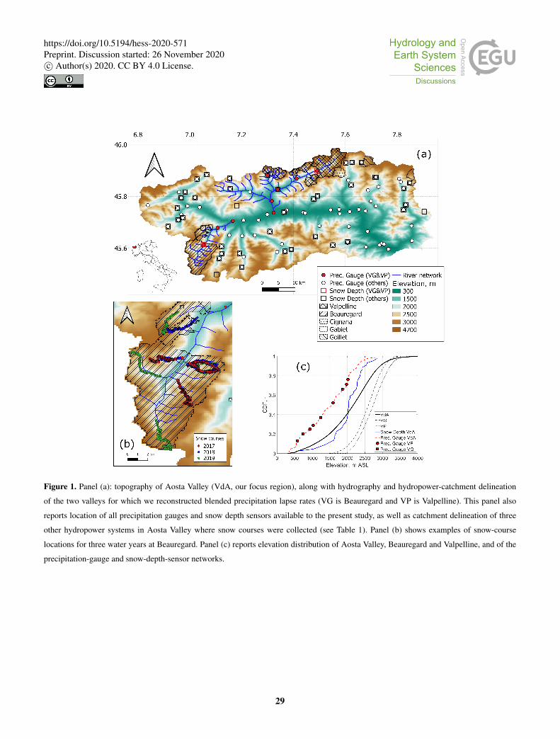
Figure 1. Panel (a): topography of Aosta Valley (VdA, our focus region), along with hydrography and hydropower-catchment delineation

of the two valleys for which we reconstructed blended precipitation lapse rates (VG is Beauregard and VP is Valpelline). This panel also

reports location of all precipitation gauges and snow depth sensors available to the present study, as well as catchment delineation of three

other hydropower systems in Aosta Valley where snow courses were collected (see Table 1). Panel (b) shows examples of snow-course

locations for three water years at Beauregard. Panel (c) reports elevation distribution of Aosta Valley, Beauregard and Valpelline, and of the

precipitation-gauge and snow-depth-sensor networks.

29


Figure 2. Average monthly cumulative precipitation (a), snow depth (b), and cumulative reconstructed streamflow (c) for Beauregard and

Valpelline. Precipitation was calculated across all gauges in the valleys of Beauregard and Valpelline (variable P , see gauge locations in

Figure 1). Snow depth was from two representative, mid-elevation sensors (elevation was ∼1860 and 1970 m ASL for the snow depth

sensor of Beauregard and Valpelline, respectively). Reconstructed streamflow refers to the hydropower catchments delineated in Figure 1.

The reference period used for these statistics varied from variable to variable due to data gaps (see Section 4.1 for details). VG and VP are

Beauregard and Valpelline, respectively.

30


Figure 3. Summary of daily precipitation (a), snow depth (b), and reconstructed streamflow (c) for Valpelline. Precipitation was calculated

across all gauges in the valleys of Valpelline (variable P , see gauge locations in Figure 1). Snow depth was from a representative, mid-

elevation sensor (elevation was ∼1970 m ASL). Reconstructed streamflow refers to the hydropower catchment delineated in Figure 1. Low,

medium, and high snow seasons were estimated based on percentiles of mean seasonal snow depth at Beauregard, which had a complete

record between water years 2008 and 2019 (Figure S14). This classification is only functional to the scopes of this paper and has no long-

term climatological meaning. Panel (d) reports the estimated precipitation-runoff relationship for both hydropower catchments, where WY P

and WY Q are water-year cumulative precipitation and reconstructed streamflow, respectively (P is systematically smaller than Q because

high-elevation headwaters are ungauged).

31


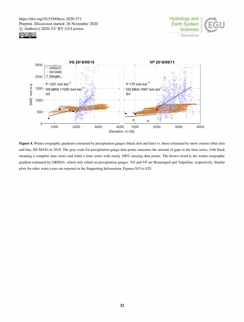
Figure 4. Winter orographic gradients estimated by precipitation gauges (black dots and line) vs. those estimated by snow courses (blue dots

and line, HS MAN) in 2018. The grey scale for precipitation-gauge data points measures the amount of gaps in the time series, with black

meaning a complete time series and white a time series with nearly 100% missing data points. The brown cloud is the winter orographic

gradient estimated by GRISO1, which only relied on precipitation gauges. VG and VP are Beauregard and Valpelline, respectively. Similar

plots for other water years are reported in the Supporting Information, Figures S15 to S25.

32


Figure 5. Annual winter orographic gradients estimated by precipitation gauges, snow courses (HS MAN), and the two snow maps assim-

ilated by Flood-PROOFS at Valpelline (a) and Beauregard (b). HS map and SWE map are the snow-depth-sensor map and the SWE map,

respectively. Details on Flood-PROOFS and these assimilated maps are reported in Section 3.3. Panels (c) and (d) show estimated orographic

gradients by snow courses as a function of mean course snow depth above 3000 m ASL (Avg. HS MAN) and survey day of the year (DOY),

respectively. ρ is Pearson’s correlation coefficient.

33


Figure 6. Orographic-enhancement factors εf for Beauregard (VG) and Valpelline (VP) across all water years as estimated using precipitation

gauges (blue and black) and snow courses (grey and light blue). The dashed lines are exponential fits between orographic-enhancement factors

and elevation, while the red line is a capped-exponential fit that was chosen to be implemented in Flood-PROOFS (Equation 1). Details on

this choice are reported in Section 4.3, while details on Flood-PROOFS are reported in Section 3. Enhancement factors are the ratio between

winter cumulative precipitation measured by gauges or estimated through snow courses above 3000 m ASL and precipitation measured by

the lowest-elevation gauge in the same valley. The orientation of triangles responds to the classification of each water year in terms of mean

snow depth, see Figure 3.

34


Figure 7. Orographic gradients of snow-depth maps derived by only using snow-depth sensors vs. those derived including high-elevation

snow courses in the calibration pool (panels a to c for Beauregard and panels e to g for Valpelline). Panels d and h show the orographic trend

of the ratio between maps derived including snow courses in the calibration pool and those derived by only using snow-depth sensors. VG

and VP are Beauregard and Valpelline, respectively.

35


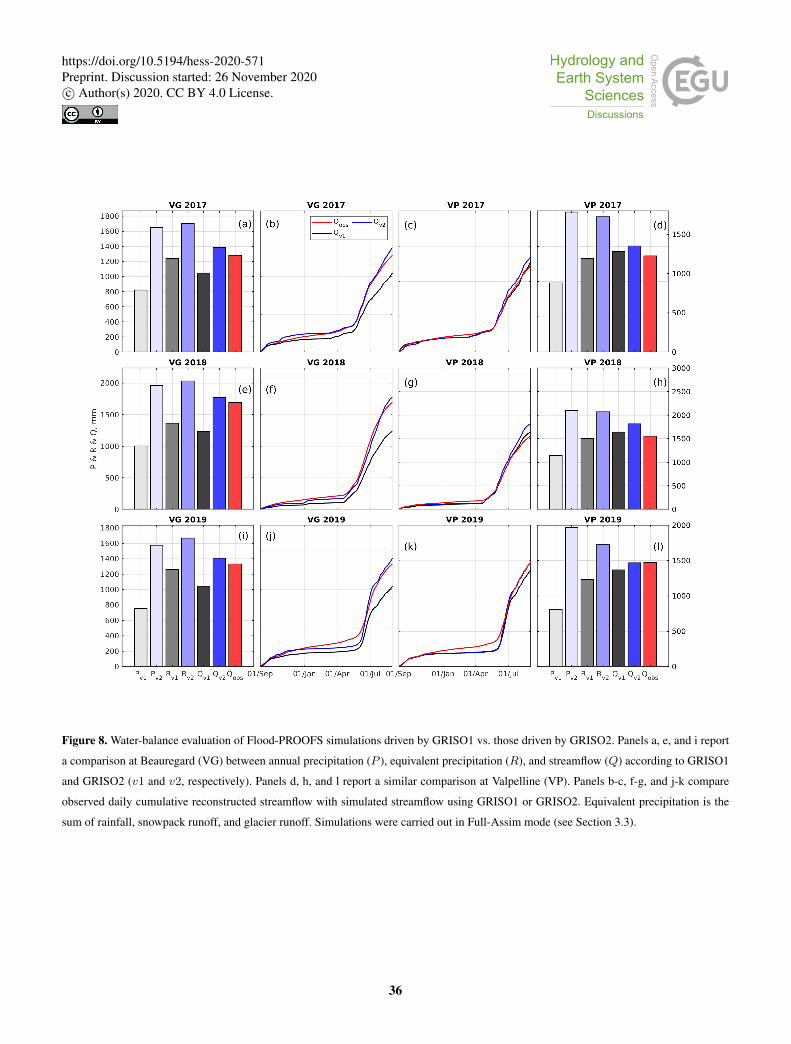
Figure 8. Water-balance evaluation of Flood-PROOFS simulations driven by GRISO1 vs. those driven by GRISO2. Panels a, e, and i report

a comparison at Beauregard (VG) between annual precipitation (P ), equivalent precipitation (R), and streamflow (Q) according to GRISO1

and GRISO2 (v1 and v2, respectively). Panels d, h, and l report a similar comparison at Valpelline (VP). Panels b-c, f-g, and j-k compare

observed daily cumulative reconstructed streamflow with simulated streamflow using GRISO1 or GRISO2. Equivalent precipitation is the

sum of rainfall, snowpack runoff, and glacier runoff. Simulations were carried out in Full-Assim mode (see Section 3.3).

36


Figure 9. Evaluation of Flood-PROOFS simulations of Snow Water Equivalent (SWE) driven by GRISO1 vs. those driven by GRISO2 (v1

and v2, respectively). Panels a, e, and i report orographic trends of model bias with respect to snow-course measured SWE at Beauregard

(VG). Panels d, h, and l report a similar comparison at Valpelline (VP). Panels b-c, f-g, and j-k compare simulated SWE using both GRISO1

or GRISO2. Simulations were carried out both in Open-Loop and in Full-Assim mode (see Section 3.3).

37


Learning about precipitation orographic enhancement from ...

Documents

Transcript of Learning about precipitation orographic enhancement from ...