PRECIPITATION PRECIPITATION

PRECIPITATION

PRECIPITATION

Precipitation occurs when 3 conditions

are met

• Atmosphere is saturated

▪ Air mass cooled by lifting ( Frontal systems, orographic

effects, convection )

• Small particles are present

▪ Dust, Aerosols, Salts ( N, S, compounds)

• Drops are big enough to reach the surface

▪ Condensation and Aggregation

SCHEMATIC OF THE

PRECIPITATION PROCESS

Water Vapor

Many droplets

decrease in size

due to evaporation Size of droplets

increase by

condensation

Droplets become heavy

enough to fall ( ~0.1mm)

Formation of Droplets

Nucleation – Vapor

condenses on aerosols

Some droplets

increase in size

due to impact and

aggregation

Larger drops break up

(3 – 5mm)

Rain Drops ( 0.1 – 3mm)

PRECIPITATION AT EARTH’S

SURFACE

Dominant factors influencing precipitation rate

• Fall velocity

• Size distribution

Terminal velocity is proportional to √diameter

▪ Atlas and Ulbrich, 1977:

v(D) = 3.86 D0.67 (D 0.8-4.0 mm)

(m/s) (mm)

Drop size Distribution

• Found by relating drop density (no. of drops/m3) with

distribution of drop sizes (mm)

Marshall-Palmer distribution

N(D) = No exp(-ΛD) where

N(D) and No = drops/m3/mm of drop diameter

Λ = mm-1 = 4.1R-0.21

No = 8000 m-3mm-1

R = Rainfall rate mm/h


SURFACE

Radar reflectivity factor (mm6/m3)

M

i ii DvDVR1

314 )()106(

3

1

319 )()1012

(

M

i iiw DvDVKE

M

i iDVZ1

61


SURFACE Drop size Distribution

• Automated instruments used – Distrometer,

Raindrop camera

Interception • Throughfall

• Stemflow

• Interception loss

Interception loss by vegetation = f(rainfall characteristics & vegetative cover)

Precipitation scavenging Mechanisms of removing aerosol from atmosphere and

delivery of atmospheric pollutants to the land.

• >50% of atmospheric moisture acidity is due to

precipitation scavenging

• Acid (sulfuric) rain: sulfur particles due to burning of

coal and oil


SURFACE

Rain gauges

• Recording type

• Non recording type

• Recording type with telemetry ( real-time

transmission)

▪ Type of Recording Rain gauges

• Weighing type

• Float and siphon

• Tipping-bucket

PRECIPITATION MEASUREMENT

▪ Weighing type rain gauge


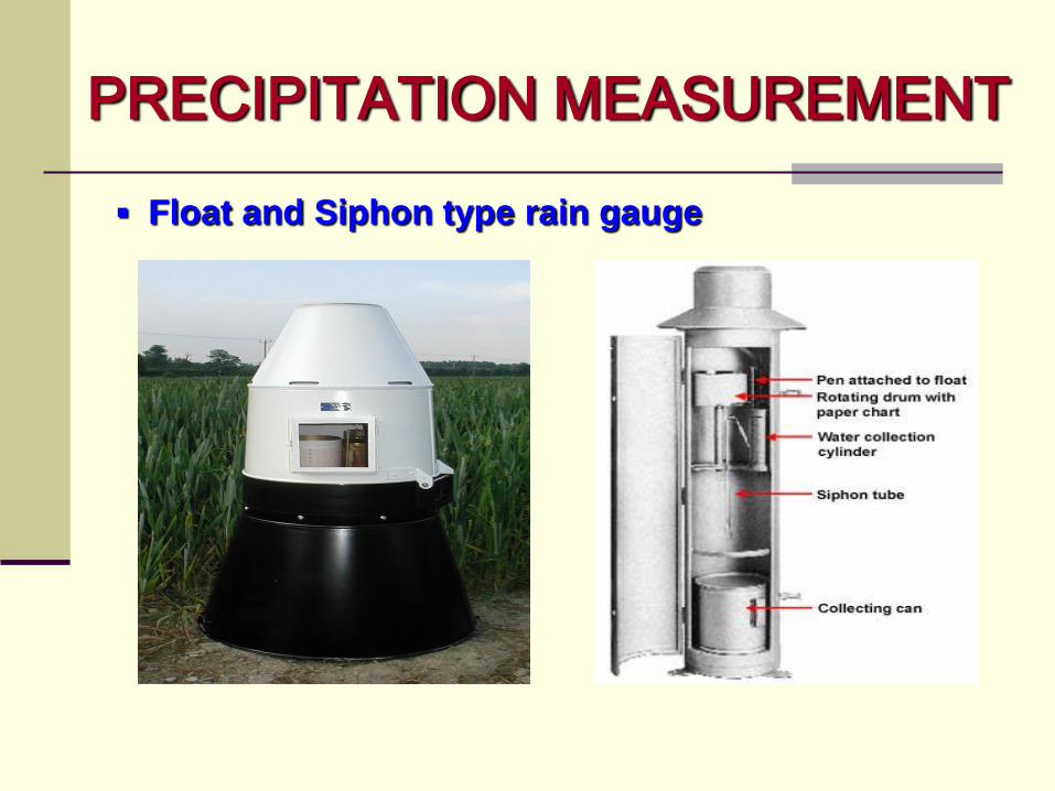
▪ Float and Siphon type rain gauge


▪ Tipping bucket type rain gauge


SPATIAL ESTIMATION OF

RAINFALL

Concept

ai = station weights Σai=1

Pi = rainfall at station i

Methods

• Arithmetic mean

• Thiessen polygon

• Isohyetal method

n

i ii PaP1

“KRIGING TECHNIQUE”

• m grid boxes mean of m estimates

n

i ij

n

i iijj

da

PdaP

1

12

1

2

)(

. j . gauge i


RAINFALL


RAINFALL

• Arithmetic mean method

Measured rainfall at six rain gauges

Watershed boundary


RAINFALL

• Arithmetic mean method

Pavg = (ΣWiPi) / ΣWi

All gauges are given an equal weight = 1

Pavg = {1.62 + 2.15 + 1.80 + 2.26 + 2.18 +1.81} /6

Pavg = 1.97 in.

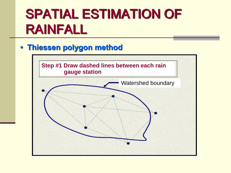
• Thiessen polygon method

Step #1 Draw dashed lines between each rain gauge station

Watershed boundary


RAINFALL



RAINFALL

Step #2 Draw the perpendicular bisector lines

Watershed boundary



RAINFALL

Step #3 Determine the area of each polygon

Watershed boundary



RAINFALL

Step #4 Calculate the average rainfall

Pavg = (ΣWiPi) / ΣWi

Pavg = {(56 x 1.62) + (150 x 2.15) + (136 x 1.80)

+(269 x 2.26) + (216 x 2.18) + (65 x 1.81)} /

(56 + 150 + 136 + 269 + 216 + 65)

Pavg = 2.08 in.

Isohyet

Area*

enclosed

(sq.km)

Net area

(sq.km)

Avg.

Prec.

(mm)

Prec. volume

(Col.3xCol.4)

127 34 34 135 4590

102 233 199 117 23283

76 534 300 89 26700

51 1041 508 64 32448

25 1541 500 38 19000

<25 1621 80 20 1600

107621

Average = 107621 / 1621 = 66 mm

* Within basin boundary


RAINFALL • Isohyetal method

RADAR MEASUREMENT OF

RAINFALL


RAINFALL

▪ Principle of Rainfall measurement by RADAR

• Electromagnetic waves released

• The waves interact with obstructions

(raindrops) in their path and send a

signal back to the radar

• Based on the reflectivity, the return

energy is digitally converted to

estimates of rainfall

Reflectivity depends on

▪ Drop size distribution

▪ Drop density

▪ Physical state

▪ Shape

▪ Aspect w.r.t. radar


RAINFALL

Attenuation • Loss of radar energy due to passage through

precipitation

Average returned power

C = constant depends on wavelength, beam shape and width, pulse

length, transmitted power, antenna gain, etc.

L = fractional signal losses by attenuation

Z = radar reflectivity factor =

r = range = distance between target and radar

M

i iDV1

61

2r

CLZP

http://images.google.co.th/imgres?imgurl=http://www.weatheronline.co.uk/daten/gifs/uk_radar_promo_v3op.gif&imgrefurl=http://www.weatheronline.co.uk/member/&h=445&w=324&sz=18&hl=th&start=1&sig2=eof11moQSJ1k-nEocAuq6g&um=1&usg=__yKyS7Bd41MJmOoVIMSHtFwoNItU=&tbnid=SphRayerF6Eq-M:&tbnh=127&tbnw=92&ei=ZaKwSJCkCZes6gP4ibj_Dw&prev=/images%3Fq%3DRAINFALL%2BRADAR%2BIMAGES%26um%3D1%26hl%3Dth

Power law models (Z-R relationships)

a and b are power law parameters

Wavelengths of 5 to 10 cm with beam width

less than 2° are used

baZR


RAINFALL

Major satellite monitoring programs for rainfall

• Global Precipitation Climatology Project (GPCP)

• Tropical Rainfall Measuring Mission (TRMM)

Mechanism used to determine rainfall

• Infrared imagery -- Radiant energy from atmosphere, land or water

is converted into temperature using Stefan-Boltzmann Law

BRIGHTNESS TEMPERATURE

Lapse rate

Cloud top height

▪ Low brightness temp high cloud top large thickness and high

probability of rainfall

▪ Relationship between cloud properties cloud-top height and rainfall

are being developed

SATELLITE MEASUREMENT

OF RAINFALL

ESTIMATING MISSING

PRECIPITATION DATA

Station average method

• Consider “n” rain gages present in a region with measured

data for a given storm event

• If data at station “X” is missing

• Then,

• Use this method when the annual rainfall of any station is within

the 10% of the average annual rainfall from the gauges

ESTIMATING MISSING

PRECIPITATION DATA Normal Ratio Method

• Used where the average annual rainfall differs considerably

between locations

PX = Missing rainfall data at “X”

NX = Annual rainfall at “X”

NA, NB, NC = Annual rainfall at A, B &C

PA, PB, PC = Rainfall for particular storm at A, B &C

CCBBAAx

C

C

x

B

B

x

A

A

x

x

PbPbPbaP

PN

NP

N

NP

N

NP

3

1

Multiple linear regression

a ≈ zero

b’s = three coefficients divided

by 3

DATA CONSISTENCY

Double mass Analysis

• It is a plot of successive cumulative annual precipitation of a

suspect gauge versus the cumulative annual precipitation of

other gauges in the same region for the same duration.

• A change in proportionality between the measurements at the

suspect station and those of the region is reflected in a

change in the slope of the trend of the plotted points

DATA CONSISTENCY

Example

• The problem is in

station E

• Find the average for

stations A to D and

then the cumulative

• Find the cumulative

for station E

DATA CONSISTENCY

• Plot cumulative E versus average cumulative A-D

DATA CONSISTENCY

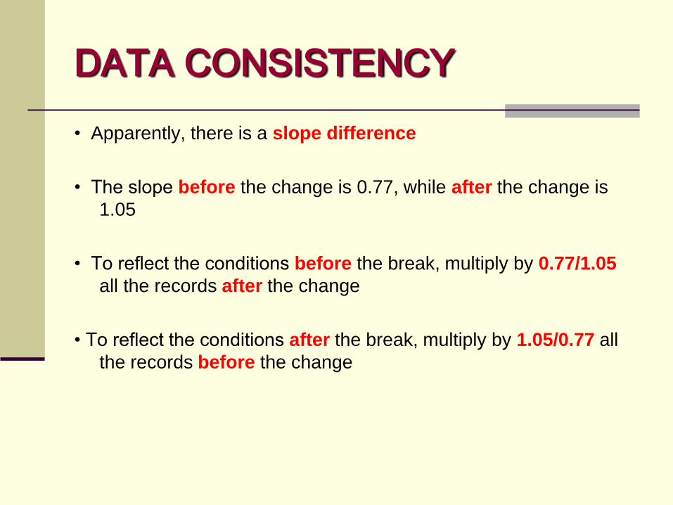
• Apparently, there is a slope difference

• The slope before the change is 0.77, while after the change is

1.05

• To reflect the conditions before the break, multiply by 0.77/1.05

all the records after the change

• To reflect the conditions after the break, multiply by 1.05/0.77 all

the records before the change

DATA CONSISTENCY

STATION E STATION E

Original Data Adjusted Data Original Data Adjusted Data

32.85 44.80 30.00 22.00

28.08 38.29 42.82 31.40

33.51 45.70 37.93 27.82

29.58 40.34 50.67 37.16

23.76 32.40 46.85 34.36

58.39 42.82 50.52 37.05

46.24 33.91 34.38 25.21

30.34 22.25 47.60 34.91

46.78 34.31

DATA CONSISTENCY

Need for rainfall frequency analysis

• Design of engineering works to control runoff

Examples – Storm sewers, Highway/Railway culverts etc

Objective of rainfall frequency analysis

To compute

• Amount of rainfall y IN duration x

Given probability p WITH return period T

pT

1

RAINFALL FREQUENCY

ANALYSIS

“Theoretically the greatest depth of precipitation

for a given duration that is physically possible

over a given size storm area at a particular

geographical location at certain time of year.”

• Three meteorological components determine

maximum precipitation possible

▪ Amount of precipitable water

▪ Rate of convergence

▪ Vertical motion

PROBABLE MAXIMUM

PRECIPITATION

MOISTURE MAXIMIZATION

AND STORM TRANSPOSITION

Data required

• Catalogue of extreme events

• Surface dew point temperatures

Precipitable water

RH = Relative humidity

q = Specific humidity

p = Pressure

p

RHeq s622.0

Moisture maximization

Surface dew point

• Moisture maximization

• Highest over a period of 50 years (WMO)

Storm transposition (Meteorologically homogeneous)

• Meteorological analysis of the storm (storm type)

• Determine transposition limits

• Apply adjustments for changes in storm location

GENERALIZED PMP

MOISTURE MAXIMIZATION

AND STORM TRANSPOSITION

WORLD’S GREATEST

OBSERVED POINT RAINFALLS Duration Depth (mm) Location Day

1 min 38 Guadeloupe 26-Nov-70

3 min 126 Bavaria 25-May-20

15 min 198 Jamaica 12-May-16

42 min 305 Holt, Mo. 22-Jun-47

2 hr 10 min 483 Rockport, W.Va July 18, 1889

9 hr 1087 Belouve, Reunion 28-Feb-64

12 hr 1340 Belouve, Reunion Feb 28-29, 1964

24 hr 1870 Cilaos, Reunion Mar 15-16, 1952

2 days 2500 Cilaos, Reunion Mar 15-17, 1952

7 days 4110 Cilaos, Reunion Mar 12-19, 1952

15 days 4798 Cherrapunji, India June 24-July 8, 1931

31 days 9300 Cherrapunji, India July 1861

2 mo 12767 Cherrapunji, India June-July 1861

6 mo 22454 Cherrapunji, India Apr-Sept 1861

1 year 26461 Cherrapunji, India Aug 1860-July 1861

2 years 40768 Cherrapunji, India 1860-1861

STATION

DURATION

MINUTES HOURS

5 15 30 1 6 24

New York, N.Y. 26 41 59 75 113 243

7/5/1973 7/10/1905 8/12/1926 8/26/1947 10/1/1913 10/8/1908

St. Louis, Mo. 22 35 65 88 148 223

3/5/1897 8/8/1923 8/8/1923 7/23/1933 7/9/1942 8/15/1946

New Orleans, La. 25 48 81 120 219 356

2/5/1955 4/25/1953 4/25/1953 4/25/1953 9/6/1929 4/15/1927

Denver, Colo. 23 40 51 56 74 166

7/14/1912 7/25/1965 7/25/1965 8/23/1921 8/23/1921 5/21/1876

San Francisco,

Calif. 8 17 21 27 59 119

11/25/1926 11/4/1918 3/4/1912 3/4/1912 10/11/1926 1/29/1881

MAXIMUM RECORDED RAINFALL

(mm) OF 5 MAJOR US CITIES

AREA

(km2)

DURATION (hr)

6 12 18 24 36 48 72

26 627a 757b 922c 983c 1062c 1095c 1148c

259 498b 668c 826c 894c 963c 988c 1031c

518 455b 650c 798c 869c 932c 958c 996c

1295 391b 625c 754c 831c 889c 914c 947c

2590 340b 574c 696c 767c 836c 856c 886c

5180 284b 450c 572c 630c 693c 721c 754c

12950 206bd 282b 358b 394c 475c 526e 620e

25900 145d 201f 257g 307g 384c 442e 541e

51800 102d 152f 201g 244g 295c 351e 447e

129500 64gh 107i 135g 160g 201g 251l 335l

259000 43h 64hk 89g 109g 150m 168j 226j

STORM DATE LOCATION

a July, 17-18,1942 Smethport. Pa.

b Sept. 8-10, 1921 Thrall, Tex.

c Sept. 3-7, 1950 Yankeetown, Fla.

d June 27-July 4, 1936 Bebe, Tex.

e June 27-July 1, 1899 Hearne, Tex.

f Apr. 12-16, 1927 Jefferson Parish, La.

g Mar. 13-15, 1929 Elba, Ala.

h May 22-26, 1908 Chattanooga, Okla.

i Apr. 15-18, 1900 Eutaw, Ala.

j July 5-10, 1916 Bonifay, Fla.

k Nov. 19-22, 1934 Millry, Ala.

l Sept. 19-24, 1967 Sombreretillo, Mex.

m Sept. 29-Oct. 3, 1929 Vernon, Fla.

MAXIMUM OBSERVED DEPTH

AREA DURATION DATA FOR US

Average Rainfall (mm)

DEPTH AREA CURVE

Depth- area curves for reducing point rainfall to obtain areal average values

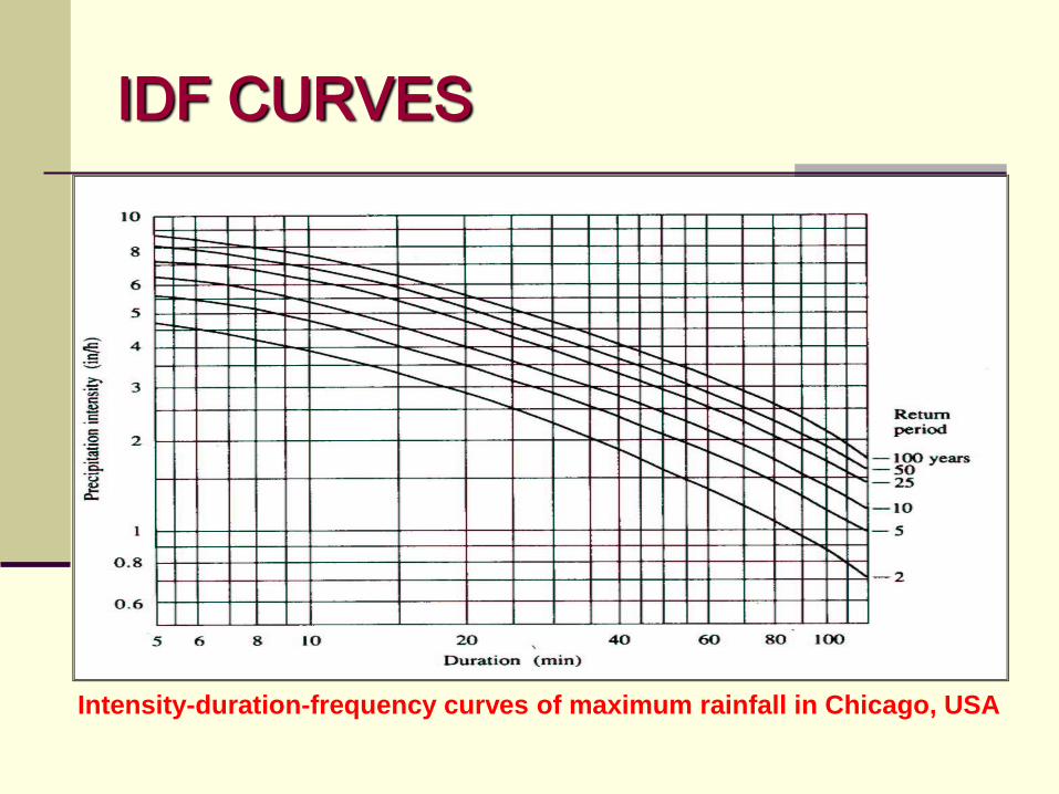
IDF CURVES

Intensity-duration-frequency curves of maximum rainfall in Chicago, USA

IDF CURVES

Intensity-duration-frequency curves for Oklahoma City

PRECIPITATION PRECIPITATION

Documents

Transcript of PRECIPITATION PRECIPITATION