Characterizing and Modelling

Precipitation in Zirconium Alloys

A thesis submitted to the University of Manchester

for the degree of

Doctor of Philosophy

in the

Faculty of Science and Engineering

2019

Zaheen D Shah

School of Natural Sciences

Department of Materials

2

Table of Contents

List of Figures ........................................................................................................................... 6

List of Tables .......................................................................................................................... 16

Abstract .................................................................................................................................. 17

Declaration ............................................................................................................................. 18

Copyright Statement .............................................................................................................. 19

Acknowledgements ................................................................................................................ 21

Abbreviations ......................................................................................................................... 24

1 Introduction ................................................................................................................... 25

1.1 Thesis Outline and Project Objectives ................................................................... 29

2 Literature Review ........................................................................................................... 30

2.1 Zirconium Alloys ..................................................................................................... 30

2.1.1 Zirconium-Tin Based Alloys ............................................................................ 31

2.1.2 Zirconium-Niobium Based Alloys ................................................................... 32

2.2 Development of Zirconium Alloy Fuel Cladding ..................................................... 32

2.2.1 Cold Pilgering ................................................................................................. 34

2.2.2 Heat Treatments ............................................................................................ 34

2.3 Second Phase Particles (SPPs) in Zirconium Alloys ................................................ 35

2.3.1 Alloying Zirconium with Tin ........................................................................... 35

2.3.2 Alloying Zirconium with Iron, Chromium and Nickel ..................................... 36

2.3.3 SPP Morphology and Distribution .................................................................. 39

2.4 SPP Characterization Techniques ........................................................................... 41

2.4.1 Scanning Electron Microscopy ....................................................................... 41

2.4.2 (Scanning) Transmission Electron Microscopy .............................................. 44

2.4.3 Atom Probe Tomography ............................................................................... 46

2.4.4 Differential Scanning Calorimetry .................................................................. 47

2.4.5 Thermoelectric Power .................................................................................... 48

2.4.6 X-ray Diffraction ............................................................................................. 50

2.5 Effect of Processing on SPPs in Zr Cladding ........................................................... 52

2.5.1 β-Quenching ................................................................................................... 52

2.5.2 Hot Extrusion .................................................................................................. 53

2.5.3 Cold Pilgering ................................................................................................. 53

2.5.4 Heat Treatments ............................................................................................ 54

3

2.5.5 The Role of SPPs in Reactor Conditions ......................................................... 58

2.6 Second Phase Particle Precipitation in the Solid State .......................................... 59

2.6.1 SPP Nucleation ............................................................................................... 59

2.6.2 SPP Growth .................................................................................................... 63

2.6.3 SPP Coarsening ............................................................................................... 66

2.7 Modelling SPP Precipitation Kinetics ..................................................................... 67

2.7.1 Johnson-Mehl-Avrami-Kolmogorov Model .................................................... 67

2.7.2 Lifshitz-Slyozov-Wagner and Kahlweit Theories ............................................ 67

2.7.3 Kampmann-Wagner Numerical Model .......................................................... 69

2.8 Summary and the Present Work ............................................................................ 72

3 Experimental Methods .................................................................................................. 75

3.1 Material .................................................................................................................. 75

3.2 Sample Preparation ............................................................................................... 75

3.2.1 Mechanical Polishing for Scanning Electron Microscopy .............................. 75

3.2.2 Electropolishing STEM Samples ..................................................................... 77

3.2.3 DSC Samples ................................................................................................... 77

3.2.4 TEP Samples ................................................................................................... 77

3.3 Scanning Electron Microscopy ............................................................................... 79

3.3.1 Energy and Angle Selective Backscatter Detector ......................................... 82

3.3.2 Electron Backscatter Diffraction .................................................................... 86

3.3.3 Energy Dispersive X-Ray Spectroscopy .......................................................... 86

3.4 Scanning Transmission Electron Microscopy ......................................................... 88

3.4.1 STEM Imaging ................................................................................................. 89

3.4.2 STEM-EDX ....................................................................................................... 89

3.5 Differential Scanning Calorimetry .......................................................................... 90

3.6 Thermoelectric Power ............................................................................................ 92

4 Experimental Characterization of Second Phase Particles ............................................ 94

4.1 Electron Microscopy .............................................................................................. 94

4.1.1 SEM ................................................................................................................ 94

4.1.2 STEM ............................................................................................................ 102

4.1.3 Comparison of SEM and STEM Characterization ......................................... 107

4.2 DSC ....................................................................................................................... 112

4.3 TEP ........................................................................................................................ 115

4.4 Summary .............................................................................................................. 117

4

5 Evolution of SPP Characteristics throughout Thermomechanical Processing ............. 121

5.1 SPP Characteristics in Zircaloy-2 and HiFi ............................................................ 121

5.2 Industrial β-quenched Material ........................................................................... 123

5.2.1 SEM Analysis ................................................................................................ 123

5.2.2 STEM Analysis .............................................................................................. 123

5.3 Industrial Hot Work, Pilger, and Anneal Stages ................................................... 126

5.3.1 SPP Evolution in Zircaloy-2 ........................................................................... 126

5.3.2 SPP Evolution in HiFi .................................................................................... 132

5.4 Effect of Thermomechanical Processes on SPP Characteristics........................... 139

5.4.1 Effect of Hot Extrusion ................................................................................. 139

5.4.2 Effect of Cold Work ...................................................................................... 142

5.4.3 Effect of Annealing ....................................................................................... 144

5.4.4 SPP Solute Distribution ................................................................................ 147

5.5 Summary .............................................................................................................. 150

6 Simulating Precipitation Kinetics in Zircaloy-2 and HiFi ............................................... 151

6.1 KWN Model Operation ......................................................................................... 151

6.2 Additional Features .............................................................................................. 153

6.2.1 Precipitation of Multiple SPPs ...................................................................... 153

6.2.2 Heterogeneous Nucleation of SPPs ............................................................. 153

6.2.3 Co-Precipitation ........................................................................................... 154

6.2.4 Particle Morphology ..................................................................................... 155

6.3 Input Parameters ................................................................................................. 155

6.3.1 Effective Solute Diffusion and Activation Energy ......................................... 155

6.3.2 SPP Molar Volume........................................................................................ 158

6.3.3 Particle Interfacial Energy ............................................................................ 159

6.3.4 Effective Nucleation Site Density ................................................................. 160

6.3.5 Matrix Solute Concentration in Equilibrium with Precipitates .................... 160

6.3.6 Average Concentration of Solute in Matrix ................................................. 165

6.3.7 Solute Concentration within Precipitates .................................................... 165

6.3.8 Heat Treatments .......................................................................................... 165

6.4 Model Calibration ................................................................................................ 165

6.4.1 Effective Interfacial Energy .......................................................................... 168

6.4.2 Nucleation Site Density ................................................................................ 172

6.4.3 Comparison with Experimental Data ........................................................... 174

5

6.5 Application of KWN Model .................................................................................. 175

6.5.1 Modelling SPP Kinetics in HiFi ...................................................................... 175

6.5.2 Application to Industrial Processing ............................................................ 177

6.6 Summary .............................................................................................................. 181

7 Conclusions .................................................................................................................. 184

7.1 SPP Characterization Techniques ......................................................................... 184

7.2 SPP Evolution throughout Thermomechanical Processing .................................. 185

7.3 Simulating SPP Kinetics in Zircaloy-2 and HiFi ..................................................... 186

8 Future Work ................................................................................................................. 188

8.1 Effect of Thermomechanical Processing on SPP Characteristics ......................... 188

8.2 Quantity of Solutes in SPPs and Matrix................................................................ 188

8.3 Modelling Zr2(Fe,Ni) kinetics ................................................................................ 189

8.4 Simulating the Effect of Deformation and Grain Growth on SPP Kinetics ........... 190

9 References ................................................................................................................... 191

Word Count: 47,120

6

List of Figures

Figure 1-1: Electricity generation by technology, adapted from [2]. ........................ 25

Figure 1-2: Operating status of different nuclear reactors worldwide, adapted from

[12]. ............................................................................................................................ 26

Figure 1-3: Schematic of fuel assemblies used in BWRs, and PWRs, adapted from [13].

.................................................................................................................................... 27

Figure 2-1: Thermomechanical processing of Zr alloy final cladding material from Zr

sponge, schematically shown with: a) a flowchart where the red boxes indicate each

the main processing stages, and b) a process map where the horizontal dashed line

represents the α-Zr to β-Zr phase transformation temperature and RT indicates room

temperature. .............................................................................................................. 33

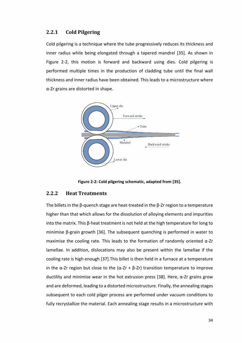
Figure 2-2: Cold pilgering schematic, adapted from [35]. ......................................... 34

Figure 2-3: Zr-Sn binary phase diagram, adapted from [56]. .................................... 36

Figure 2-4: Binary phase diagrams at the Zr-rich end where: a) shows Zr-Fe (where α

and β represent α-Zr and β-Zr respectively while ρ represents either tetragonal Zr2Fe

precipitate or orthorhombic Zr3Fe precipitate), adapted from [40], b) shows Zr-Cr

(where α, β, and ρ represent α-Zr, β-Zr and Zr(Fe,Cr)2 precipitate respectively),

adapted from [40], and c) shows Zr-Ni (where α and β represent α-Zr and β-Zr

respectively), adapted from [60]. .............................................................................. 37

Figure 2-5: Unit cell and lattice parameters [49] of: a) Zr(Fe,Cr)2, and b) Zr2(Fe,Ni) ,

adapted from [64]. ..................................................................................................... 38

Figure 2-6: Different SPP types identified in Zry-2 using (a) bright field imaging, and

EDX to map (b) Zr, (c) Sn, (d) Fe, (e) Cr and (f) Ni in a scanning transmission electron

microscope [67]. ......................................................................................................... 39

Figure 2-7: Schematic of SPP size and shapes in Zry-2, adapted from [61]. .............. 40

Figure 2-8: SEM imaging of SPPs where: a) shows the electropolishing and chemical

polishing technique, b) shows a BSE image of SPPs in Zry-2, and c) illustrates the

obtained cumulative number of particles per mm2 that are larger than the given SPP

size. Adapted from [66]. ............................................................................................. 43

7

Figure 2-9: PSD of SPPs in: a) recrystallized Zry-2, and b) recrystallized Zry-2 subject

to 1000 °C β-heat treatment and water quench, 50 % cold reduction and anneal at

600 °C for 2 hr, adapted from [17]. ............................................................................ 45

Figure 2-10: APT reconstruction of irradiation-induced precipitates with Fe and Cr,

adapted from [67]. ..................................................................................................... 47

Figure 2-11: Phase transformation upon heating in Zr-Nb(FeSn) alloys where: a)

shows the temperature of β-Nb dissolution, and b) shows the correlation between β-

Nb content and measured enthalpy, adapted from [89]. ......................................... 48

Figure 2-12: TEP evolution in α-quenched Zry-2 is heat-treated at 450 °C – 600 °C with

varying times, adapted from [94]. ............................................................................. 50

Figure 2-13: Synchrotron radiation diffraction pattern of Zry-2 with 𝛸CAP of 1 ×

10−16 hr, adapted from [49]. ..................................................................................... 51

Figure 2-14: PSD of Zr-0.85Sn-0.4Nb-0.1Cr-0.05Cu alloy annealed at 600 °C / 0.5 hr,

650 °C / 30 hr, and 700 °C / 30 hr, adapted from [72]. .............................................. 54

Figure 2-15: PSD of SPPs in Zry-4 where: a) illustrates the distribution of SPPs from

different 𝛸CAP conditions, and b) shows the evolution of SPP size ranges with CAP,

adapted from [101]. ................................................................................................... 56

Figure 2-16: Effect of 𝛸CAP on SPP size distribution in Zry-2, adapted from [43] . ... 57

Figure 2-17: Precipitation phase transformation in simple binary alloy where: β is the

single phase, α is the metastable supersaturated solid solution, ϕ is the precipitate,

T is temperature and cB is the concentration of the “B” phase. Adapted from [121].

.................................................................................................................................... 59

Figure 2-18: Gibbs free energy as a function of particle size for solid phase

precipitation, adapted from [121]. ............................................................................ 61

Figure 2-19: Gibbs free energy for heterogeneous (∆𝐺het) and homogeneous (∆𝐺hom)

nucleation as a function of particle size, adapted from [121]. .................................. 63

Figure 2-20: Schematic illustrating the effect that the radius of curvature of a particle

has on the free energy (G) of the system (Gibbs-Thomson effect) and the solute

concentration in the matrix adjacent to the particle (XB). Particles with differing radii

of curvature, residing in the matrix (with a free energy, Gα), have different interfacial

energies. A smaller particle (radius of curvature, r2) has a higher interfacial energy

than that for the larger particle (radius of curvature r1). The smaller particle therefore

8

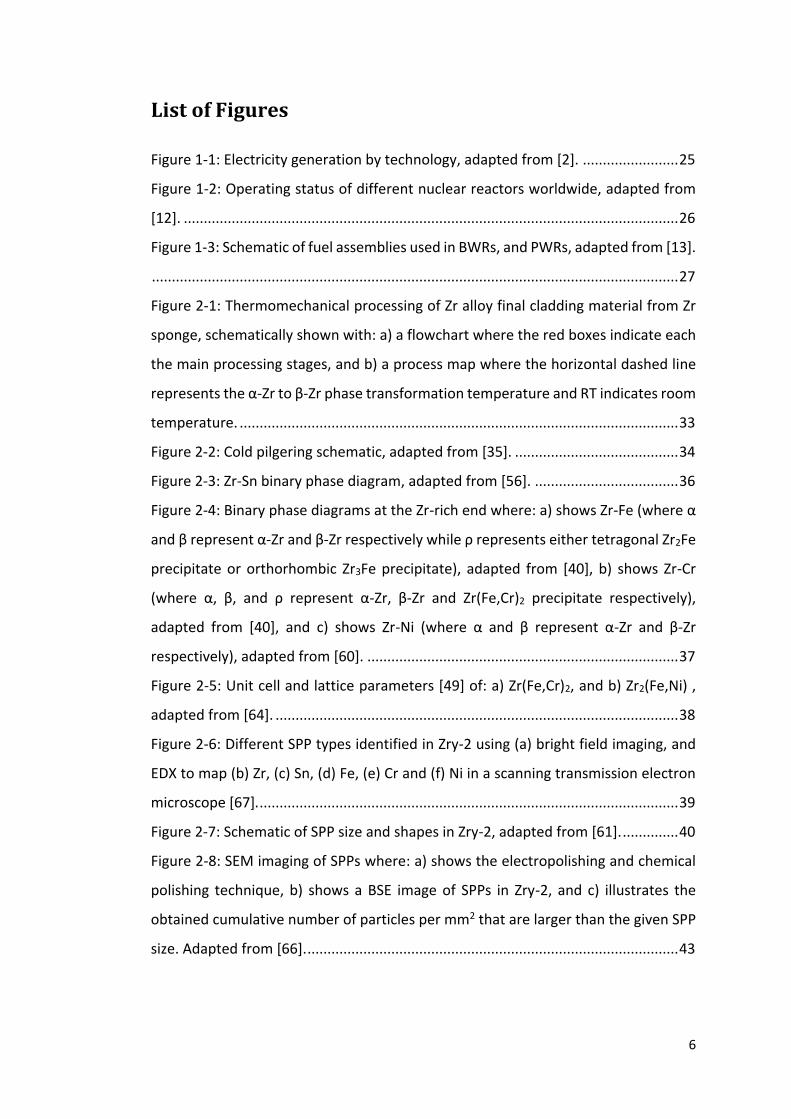
has a larger free energy and thus has a larger solute concentration adjacent to it in

the matrix (X2) than that associated to the larger particle (X1). Adapted from [121].

.................................................................................................................................... 65

Figure 2-21: SPP growth rate affected by: a) interfacial growth rate and interface

type, and (b) solute diffusion to and along grain boundaries, adapted from [121]. . 66

Figure 2-22: Comparison of LSW size distribution and experimental γ’ PSD in Ni-8.74Ti

heat treated at 692 °C / 1455 min, adapted from [123, 128]. ................................... 68

Figure 2-23: KWN model developed by Robson [134] used to predict the evolution of

SPP characteristics where: (a) shows the predicted precipitate dimension and spacing

when aged at 500 °C compared against data from [154] and, (b) shows the predicted

matrix Nb evolution against DSC and TEP from [155] and [156]. Adapted from [134].

.................................................................................................................................... 71

Figure 2-24: Simulated evolution of characteristics of Zr(Fe,Cr)2 particles in Zry-4 at

307 °C with and without irradiation at a displacement rate of 15 dpa/year where: (a)

shows particle volume fraction and matrix solute level and, (b) shows particle

number density and mean radius. Adapted from [150]. ........................................... 72

Figure 3-1: Hydrocarbon contamination and presence of colloidal silica particles in

SEM image. ................................................................................................................. 76

Figure 3-2: β-heat treatment and quench temperature profile used for TEP samples.

.................................................................................................................................... 78

Figure 3-3: SEM configuration where: a) illustrates the schematic of the whole SEM

column, and b) illustrates the schematic of the objective lens system, adapted from

[163]. .......................................................................................................................... 80

Figure 3-4: Signals produced in interaction volume generated in sample. ............... 81

Figure 3-5: Sample interaction volume size with an accelerating voltage of: a) 3 keV,

and b) 20 keV. ............................................................................................................ 82

Figure 3-6: Schematic of SEM column where the in-lens detector is used to detect

low voltage SEs and the energy selective backscatter detector is used to detect high

energy BSEs, adapted from [165]. ............................................................................. 83

Figure 3-7: SE and BSE radial distributions in the plane of the in-lens detector [166].

.................................................................................................................................... 83

9

Figure 3-8 Diagrams illustrating the BSE distribution and their associated energies in

Zry-2 at accelerating voltages of: a) 2 keV, c) 2.5 keV, e) 3 keV, and g) 3.5 keV. The

vertical dashed line indicates the filter grid voltage of 1500 eV. The simulated BSE

interaction volumes in Zry-2 show BSE energies (as a percentage of the incident

electron energy) as a function of position at accelerating voltages of: b) 2 keV, d) 2.5

keV, f) 3 keV, and h) 3.5 keV. ..................................................................................... 85

Figure 3-9: Schematic of characteristic x-rays where: a) shows how x-rays are

generated, and b) illustrates the classification of characteristic x-rays. It should be

noted that the atom in this figure is based on the Bohr model of the atom where the

inner to outer shells are labelled K, L, M, and N. Adapted from [167]. ..................... 87

Figure 3-10: Schematics of different DSC types where: a) shows a heat flux DSC, and

b) shows a power conpemsation DSC [175]. ............................................................. 91

Figure 3-11: Phase transformations identfied in Zr-2.5wt%Nb: a) when water

quenched and subsequently annealed [89], and b) shown in the Nb-Zr phase diagram

[176]. .......................................................................................................................... 91

Figure 3-12: TEP set-up: a) shown schematically [180], and b) TechLab instrument

with hot and cold junctions. ...................................................................................... 93

Figure 4-1: BSE image of SPPs in HiFi with associated EDX and EBSD of the different

SPP types. ................................................................................................................... 95

Figure 4-2: Backscatter coefficient: a) as a function of atomic number at an

accelerating voltage above 5 keV, and b) as a function of accelerating voltage (less

than 2 keV) for different materials, adapted from [73]. ............................................ 96

Figure 4-3: ESB image and associated EDX of SPPs in Zry-2. ..................................... 97

Figure 4-4: PSD of SPPs in Zry-2 final cladding material where: a) shows the effective

particle size, and b) shows the true particle size. The error bars on the red histogram

bars and cyan histogram bars show the standard error of the Zr(Fe,Cr)2 number

density and Zr2(Fe,Ni) number density respectively. The error bar on the horizontal

red line and on the horizontal orange line are the standard errors of the mean

Zr(Fe,Cr)2 size and mean Zr2(Fe,Ni) size respectively. The class width was determined

using Equation 4-6 from Gros and Wadier [107]. ...................................................... 99

10

Figure 4-5: Schematic illustrating the contribution that SPPs < 18 nm in size have to

BSE signal where the SPP is: a) present on the sample surface, and b) present under

the sample surface. .................................................................................................. 100

Figure 4-6: Cubic volume containing randomly oriented features, adapted from [185].

.................................................................................................................................. 101

Figure 4-7: STEM analysis of SPPs in Zry-2 where electron imaging is performed using:

a) STEM-BF, and b) STEM-HAADF. Associated STEM-EDX is performed where: c)

shows the Zr map, d) shows the Cr/Ni map, and e) shows the Fe map. Raw counts of

STEM-EDX are shown in: f) for Cr-rich SPP, and g) for Ni-rich SPP. ......................... 103

Figure 4-8: Mass-thickness contrast masking the presence of small Zr(Fe,Cr)2 particles

surrounding the larger Zr2(Fe,Ni) particle in industrially β-quenched HiFi. ............ 104

Figure 4-9: Thickness variation in electropolished foil. ........................................... 104

Figure 4-10: Foil thickness measurement in STEM where: a) schematically illustrates

method, and b) shows an electron image with the two ends of the through-thickness

hole. .......................................................................................................................... 105

Figure 4-11: Diffraction pattern of basal plane in Zry-2. ......................................... 108

Figure 4-12: Comparison of PSDs and cumulative size distributions in HiFi at the

intermediate anneal stage using SEM and STEM where: a) shows the Zr(Fe,Cr)2 PSD,

b) shows the Zr(Fe,Cr)2 cumulative size distribution, c) shows Zr2(Fe,Ni) PSD, and d)

shows the Zr2(Fe,Ni) cumulative size distribution. The error bars on the pink

histogram bars and blue histogram bars show the standard error of the number

density of both SPP types obtained using SEM and STEM imaging respectively. The

error bar on the horizontal red line and on the horizontal orange line are the standard

errors of the mean size for both SPP types obtained using SEM and STEM imaging

respectively. The class width was determined using Equation 4-6 from Gros and

Wadier [107]. ........................................................................................................... 111

Figure 4-13: DSC and DDSC of industrially β-quenched Zry-2. ................................ 113

Figure 4-14: DSC and DDSC of industrially β-quenched HiFi.................................... 114

Figure 4-15: Variation of TEP against isothermal heat treatment time of β-quenched

Zry-2 and HiFi relative to its β-quenched reference where: a) shows β-quenched Zry-

2 heat treated at 600 °C, b) shows β-quenched Zry-2 heat treated at 700 °C, c) shows

β-quenched HiFi heat treated at 600 °C, and d) shows β-quenched HiFi heat treated

11

at 700 °C. The error bars at each data point show the standard error of the mean of

all TEP measurements produced at each heat treatment condition. ...................... 116

Figure 5-1: SPP size distributions of Zry-2 and HiFi for: a) Zr(Fe,Cr)2, and b) Zr2(Fe,Ni)

& cumulative density distributions for both alloys for: c) Zr(Fe,Cr)2, and d) Zr2(Fe,Ni).

The mean particle size of both SPP types are shown as vertical lines. SPP imaging is

performed using the SEM. ....................................................................................... 122

Figure 5-2: ESB image of β-quenched HiFi where the passive oxide layer dominates

the surface. .............................................................................................................. 123

Figure 5-3: Presence of SPPs in β-quenched Zry-2 where: a) shows the STEM-BF

image, b) shows the associated STEM-EDX map for Fe, and c) shows the associated

STEM-EDX map for Cr and Ni. SPPs can also form on dislocations as shown in: d) with

a STEM-BF image of the highlighted region, e) shows the associated STEM-EDX map

for Fe, and f) shows the associated STEM-EDX map for Cr and Ni. ......................... 124

Figure 5-4: PSDs of SPPs observed in β-quenched: a) Zry-2, and b) HiFi. ................ 125

Figure 5-5: Evolution of SPP characteristics throughout thermomechanical processing

in Zry-2 cladding material at the β-quench stage (using STEM imaging), and from the

hot work stage to the final stage (using SEM imaging) where: a) shows SPP volume

fraction, b) shows mean SPP size, and c) shows SPP number density (axis breaks are

used to illustrate the high SPP number density present at the β-quench stage). ... 127

Figure 5-6: Size distributions of SPPs in the following processing stages of Zry-2

material: a) PSD at the hot work stage, b) cumulative number density at the hot work

stage, c) PSD at the intermediate pilger stage, d) cumulative number density at the

intermediate pilger stage, e) PSD at the intermediate anneal stage, and f) cumulative

number density at the intermediate anneal stage. ................................................. 131

Figure 5-7: Size distributions of SPPs in the following processing stages of Zry-2

material: a) PSD at the final pilger stage, b) cumulative number density at the final

pilger stage, c) PSD at the final anneal stage, and d) cumulative number density at

the final anneal stage. .............................................................................................. 132

Figure 5-8: Evolution of SPP characteristics throughout thermomechanical processing

in HiFi cladding material at the β-quench stage (using STEM imaging), and from the

hot work stage to the final stage (using SEM imaging) where: a) shows SPP volume

12

fraction, b) shows mean SPP size, and c) shows SPP number density (axis breaks are

used to illustrate the high SPP number density present at the β-quench stage). ... 134

Figure 5-9: Size distributions of SPPs in the following processing stages of HiFi

material: a) PSD at the hot work stage, b) cumulative number density at the hot work

stage, c) PSD at the intermediate pilger stage, d) cumulative number density at the

intermediate pilger stage, e) PSD at the intermediate anneal stage, and f) cumulative

number density at the intermediate anneal stage. ................................................. 137

Figure 5-10: Size distributions of SPPs in the following processing stages of HiFi

material: a) PSD at the final pilger stage, b) cumulative number density at the final

pilger stage, c) PSD at the final anneal stage, d) cumulative number density at the

final anneal stage. .................................................................................................... 139

Figure 5-11: Schematic showing the potential mechanism for SPP evolution

throughout the hot extrusion process where the red particles represent Zr(Fe,Cr)2,

the blue particles represent Zr2(Fe,Ni) , and the black lines represent grain

boundaries. Grain growth takes place throughout the extrusion process. SPPs grow

and coalesce during the prior extrusion heat treatment. During hot extrusion, smaller

SPPs dissolve and solutes distribute throughout the matrix, leading the SPP

growth/coarsening and nucleation of small SPPs. Grain distortion is also present the

extrusion process. Subsequent air cooling lead to further grain growth and SPP

coarsening. ............................................................................................................... 140

Figure 5-12: ESB images taken on the SEM of SPPs at the hot work stage in: a) Zry-2,

and b) HiFi. ............................................................................................................... 141

Figure 5-13: SPP clustering at the intermediate pilger stage in Zry-2. .................... 143

Figure 5-14: The effect of CAP on mean SPP size in Zry-2 production cladding material,

adapted from [44]. ................................................................................................... 145

Figure 5-15: Schematic showing the effect of annealing on solute diffusion where cθ

is the solute concentration, φ resembles a SPP, cαφθ is the solute concentration at the

particle/matrix interface, v1 and v2 are the velocities of SPP growth/dissolution of

the two SPPs, and Jθ is the solute concentration gradient between the small and large

SPPs. Adapted from [123]. ....................................................................................... 146

Figure 5-16: Amalgamation of two Zr2(Fe,Ni) particles in HiFi at the intermediate

anneal stage. ............................................................................................................ 147

13

Figure 5-17: Solute distribution in SPPs at the intermediate anneal stage. ............ 147

Figure 5-18: Variation in solute ratio (obtained using STEM-EDX) with SPP size at the

intermediate pilger stage where: a) shows Fe/Ni and Fe/Cr ratios in Zry-2, and b)

shows Fe/Ni and Fe/Cr ratios in HiFi in Zr2(Fe,Ni) and Zr(Fe,Cr)2 respectively. ....... 149

Figure 5-19: Variation in solute ratio (obtained using STEM-EDX) with SPP size where:

a) shows Fe/Ni and Fe/Cr ratios in Zry-2 at the intermediate pilger and intermediate

anneal stages, b) shows Fe/Ni and Fe/Cr ratios in HiFi at the intermediate pilger and

intermediate anneal stages...................................................................................... 149

Figure 6-1: Operation of the KWN model, adapted from [133]. ............................. 151

Figure 6-2: Reallocation of particles from size class 2 to classes 3-5 after the

application of growth rates vL and vU where L and U are the lower and upper edges

of the size class, adapted from [131]. ...................................................................... 152

Figure 6-3: Lattice diffusivity of Fe, Cr, and Ni in α-Zr in Zry-2 with temperature. . 157

Figure 6-4: Diffusivity vs. temperature of 𝐷Crα Zry−2

from Pande et al. [190], and 𝐷effFe+Cr

from Massih and Jernkvist [151] without the diffusivity ratio for Cr along grain

boundaries relative to that within grains in α-Zr. .................................................... 158

Figure 6-5: Zr-rich end of experimental Zr-Fe-Cr phase diagram, adapted from [40].

.................................................................................................................................. 161

Figure 6-6: Correlation between the ln(c∞) and 1 𝑇⁄ for (Fe+Cr) solutes. ............... 162

Figure 6-7: Zr-Cr phase diagram, adapted from[192]. ............................................. 162

Figure 6-8: Concentration of solutes in the matrix in equilibrium with SPPs in the Zr-

Cr (taken from Okamoto [192] and JMatPro simulations [188]) and Zr-Fe-Cr (taken

from Charquet et al. [40] and JMatPro simulations [188]) systems at the Zr-rich end.

.................................................................................................................................. 163

Figure 6-9: Concentration of solutes in the matrix in equilibrium with SPPs in the Zr-

Ni (taken from Kirkpatrick and Larsen [60], Zr-Fe-Cr (taken from Charquet et al. [40])

and Zr-Fe-Ni (taken from JMatPro [188]) systems at the Zr-rich end. .................... 164

Figure 6-10: PSD of SPPs in: a) Zry-2, and b) HiFi after the β-quench stage with a

cooling rate of approximately 1500 °C/s. PSDs were obtained using STEM imaging.

.................................................................................................................................. 166

14

Figure 6-11: PSDs of Zr(Fe,Cr)2 and Zr2(Fe,Ni) in β-quenched Zry-2, subsequently

isothermally heat treated at: a) 600 °C / 20 hr, and b) 700 °C / 2hr. PSDs are also

shown of SPPs in β-quenched HiFi, isothermally heat treated at: c) 600 °C / 10 hr, and

d) 700 °C / 1 hr. PSDs were obtained using SEM imaging. ...................................... 168

Figure 6-12: SPP volume fraction of Zry-2 isothermally heat-treated at 600 °C where:

a) shows the comparison between TEP results, the un-calibrated simulated total SPP

volume fraction, and total SPP volume fraction obtained from SEM imaging after a

600 °C / 20 hr heat treatment (where the TEP and total SPP volume fraction axes are

freely scaled), and b) shows the un-calibrated simulated volume fraction of both SPP

types in addition to experimentally obtained SPP volume fractions. The SPP volume

fraction of Zry-2 isothermally heat-treated at 700 °C is presented where: c) shows the

comparison between TEP results, the un-calibrated simulated total SPP volume

fraction, and total SPP volume fraction obtained from SEM imaging after a 700 °C /

20 hr heat treatment (where the TEP and total SPP volume fraction axes are freely

scaled), and d) shows the un-calibrated simulated volume fraction of both SPP types

in addition to experimentally obtained SPP volume fractions. ............................... 170

Figure 6-13: Predicted evolution of Zr(Fe,Cr)2 characteristics in Zry-2 with time, for

varying particle interfacial energy values, when subject to a 700 °C / 10 hr heat

treatment with: a) mean particle radius, b) nucleation rate, c) mean solute

concentration in the matrix, and d) volume fraction. The vertical line in each plot

shows the time at 2 hr (i.e. the time taken to reach the onset of coarsening identified

when β-quenched Zry-2 is heat treated at 700 °C). ................................................. 172

Figure 6-14: Predicted evolution of Zr(Fe,Cr)2 characteristics with time, for varying

nucleation site density values, when subject to a 700 °C / 10 hr heat treatment with:

a) mean particle radius, b) nucleation rate, c) mean solute concentration in the

matrix, and d) volume fraction. The vertical line in each plot shows the time at 2 hr

(i.e. the time taken to reach the onset of coarsening identified when β-quenched Zry-

2 is heat treated at 700 °C). ..................................................................................... 173

Figure 6-15: Predicted evolution of the total SPP volume fraction in Zry-2 compared

with TEP data and total SPP volume fraction obtained using SEM imaging at: a)

600 °C, and b) 700 °C. The predicted mean radius of Zr(Fe,Cr)2 and Zr2(Fe,Ni) is also

15

compared to that obtained at the onset of SPP coarsening using the SEM at: c)

600 °C, and d) 700 °C. .............................................................................................. 175

Figure 6-16: Predicted evolution of the total SPP volume fraction in HiFi compared

with TEP data and total SPP volume fraction obtained using SEM imaging at: a)

600 °C, and b) 700 °C. The predicted mean radius of Zr(Fe,Cr)2 and Zr2(Fe,Ni) is also

compared to that obtained at the onset of SPP coarsening using the SEM at: c)

600 °C, and d) 700 °C. .............................................................................................. 177

Figure 6-17: Schematic of thermal history with hot anneal, intermediate anneal, and

final anneal stages. ................................................................................................... 178

Figure 6-18: Evolution of both SPP types in Zry-2 throughout a simulated thermal

history where the following characteristics are shown: a) mean particle radius, b)

particle number density, c) particle nucleation rate, d) mean solute concentration in

the matrix, e) SPP volume fraction and equilibrium SPP volume fraction, and f) the

PSD after the final anneal. The hot anneal, intermediate, and final anneal stages are

abbreviated to: HA, IA, and FA. ................................................................................ 181

16

List of Tables

Table 1-1: Different nuclear reactor types and operating conditions [5–11]. ........... 26

Table 2-1: Experimental technique capabilities for SPP characterization. ................ 41

Table 2-2: Particle growth kinetics predictions using Kahlweit’s theory [40, 107]. .. 68

Table 3-1: Composition of Zry-2 and HiFi (wt%). ....................................................... 75

Table 3-2: Simulated interaction volume size. ........................................................... 84

Table 3-3: Characteristic x-ray energy lines (keV) [174]. ........................................... 88

Table 3-4: Electron wavelength as a function of accelerating voltage. ..................... 88

Table 4-1: SPPs characteristics of Zr(Fe,Cr)2 and Zr2(Fe,Ni) in HiFi at the intermediate

anneal stage, obtained using SEM and STEM. ......................................................... 111

Table 4-2: Experimental technique capabilities for SPP characterization in Zry-2 and

HiFi. ........................................................................................................................... 118

Table 5-1: SPPs characteristics in industrially β-quenched Zry-2 and HiFi. ............. 126

Table 5-2: Largest Zr(Fe,Cr)2 and Zr2(Fe,Ni) size in Zry-2 and HiFi at each processing

stage. ........................................................................................................................ 144

Table 5-3: Fe/Ni and Fe/Cr solute ratios respectively in Zr2(Fe,Ni) and Zr(Fe,Cr)2 in Zry-

2 and HiFi at the intermediate pilger stage, the intermediate anneal stage, and under

equilibrium conditions at the intermediate temperature as predicted by JMatPro

[188]. ........................................................................................................................ 148

Table 6-1: Proportion of SPPs, by number, formed in the grain interior and on grain

boundaries in Zry-2 and HiFi, isothermally heat treated at 600 °C or 700 °C.......... 154

Table 6-2: Proportion of SPPs precipitating from one another in Zry-2 and HiFi when

isothermally heat treated at 600 °C or 700 °C from the β-quenched condition. .... 155

Table 6-3: (Fe+Cr) solute concentration and temperature data points along solvus.

.................................................................................................................................. 161

Table 6-4: SPP characteristics of Zr(Fe,Cr)2 and Zr2(Fe,Ni) in Zry-2 and HiFi after the β-

quench stage with a cooling rate of approximately 1500 °C/s. ............................... 166

17

Abstract

Zirconium alloys (Zr) are used in the nuclear industry in components present in light- and heavy-water reactors cores. Zr alloys experience corrosion, which is thought to be minimised by adding alloying elements such as iron (Fe), chromium (Cr), and nickel (Ni). This leads to the formation of second phase particles (SPPs): Zr(Fe,Cr)2 and Zr2(Fe,Ni). SPP size, number density, and distribution are thought to be affected by the thermomechanical processing applied to Zr alloys. Therefore, it is important to understand how processing affects these SPP characteristics, which in turn is thought to affect Zr alloy corrosion performance. Such characteristics can be predicted by modelling SPP kinetics. This has the potential to replace expensive experimental procedures when determining SPP characteristics for optimal Zr alloy performance.

In this study, SPPs in Zircaloy-2 and HiFiTM – a novel high-Fe alloy – fuel cladding material were analysed using different characterization techniques to determine SPP characteristics and technique limitations. Scanning electron microscopy (SEM) and scanning transmission electron microscopy (STEM) directly counted the number of both SPP types. SEM imaging produced reliable particle size distributions, enabling a large number of particles to be counted to give good statistics, although resolution is limited. STEM imaging instead has a higher resolution and enables detailed analysis of SPP chemistry, though fewer SPPs can be counted in a reasonable time-frame. Differential scanning calorimetry (DSC) and thermoelectric power (TEP) are capable of tracking SPP kinetics when the alloys are heat-treated. SPP dissolution temperatures are identified using DSC although their endothermic peaks cannot be separated and thus it is not suitable for discriminating between SPP phases. Changes in solute concentration with further heat treatments were ascertained using TEP, providing a measurement of the aggregate SPP volume fraction, and was used to rapidly determine the onset time for important microstructural events, such as the start of coarsening dominated kinetics.

The evolution of SPP characteristics throughout processing was determined using SEM and STEM. SPPs are located on grain boundaries and dislocations during the β-quench stage where SPP nucleation and growth are present. These regimes are complete during the hot work stage with SPP coarsening being dominant. The highest SPP volume fraction is obtained at this stage with subsequent cold pilger and intermediate temperature anneal stages having a similar SPP volume fraction. The hot work stage deforms the microstructure where SPPs are present within the grain interior and on grain boundaries. Cold pilgering decreases the mean SPP size and increases SPP number density as larger SPPs break up. Annealing is dominated by SPP coarsening where the mean SPP size increases and SPP number density decreases.

A physical kinetics model, based on classical nucleation, growth and coarsening theories, has been developed to capture the evolution of SPP characteristics when subject to thermal exposure. Model calibration is based on the TEP data and mean SPP size obtained at certain heat treatments. This model, calibrated on data from Zircaloy-2, has been applied directly to predict SPP kinetics in HiFi, demonstrating a good predictive capability. In addition, this model has been applied to a thermal history used in the production of Zr cladding, enabling the dominant SPP evolution process to be determined throughout processing and confirming that coarsening is the main operating mechanism for all annealing stages.

18

Declaration

No portion of the work referred to in the thesis has been submitted in support of an

application for another degree of qualification of this or any other university or other

institute of learning.

19

Copyright Statement

The author of this thesis (including any appendices and/or schedules to this thesis)

owns certain copyright or related rights in it (the “Copyright”) and s/he has given The

University of Manchester certain rights to use such Copyright, including for

administrative purposes.

Copies of this thesis, either in full or in extracts and whether in hard or electronic

copy, may be made only in accordance with the Copyright, Designs and Patents Act

1988 (as amended) and regulations issued under it or, where appropriate, in

accordance with licensing agreements which the University has from time to time.

This page must form part of any such copies made.

The ownership of certain Copyright, patents, designs, trademarks and other

intellectual property (the “Intellectual Property”) and any reproductions of copyright

works in the thesis, for example graphs and tables (“Reproductions”), which may be

described in this thesis, may not be owned by the author and may be owned by third

parties. Such Intellectual Property and Reproductions cannot and must not be made

available for use without the prior written permission of the owner(s) of the relevant

Intellectual Property and/or Reproductions.

Further information on the conditions under which disclosure, publication and

commercialisation of this thesis, the Copyright and any Intellectual Property

and/or Reproductions described in it may take place is available in the University IP

Policy (see http://documents.manchester.ac.uk/DocuInfo.aspx?DocID=24420), in

any relevant Thesis restriction declarations deposited in the University Library, The

University Library’s regulations (see

http://www.library.manchester.ac.uk/about/regulations/) and in The University’s

policy on Presentation of Theses.

20

“Your mind is like this water, my friend.

When it is agitated, it becomes difficult to see.

But if you allow it to settle, the answer becomes clear.”

(Grand Master Oogway in DreamWorks Animation’s Kung Fu Panda, 2008)

21

Acknowledgements

Starting with the formal acknowledgements, I would like to thank Prof. Joe Robson

and Prof. Michael Preuss for their services to this project over the three and a half

years. Without the structure, this thesis would most likely be a mess with ideas flying

everywhere! A big thank you also goes to Ken Gyves and Dave Strong for their help

with sample preparation. In addition, listening to their stories about things that shall

never be mentioned again is the only thing that let me enjoy the monotonous task of

creating shiny metal samples week after week for three years! You know what I mean

if you have had to this. Credit also goes to Claire Hinchcliffe, formerly at the Advanced

Metallic Systems (AMS) CDT, who gave the opportunity to a student with limited

knowledge of metallurgy the chance to show the world (i.e. the AMS 2015 cohort,

and anyone who ever decided to listen to me) that zirconium is not all that bad.

I am also thankful for the help that I have got for some of the experimental work.

Firstly, I am grateful for the help that Allan Harte, formerly University of Manchester

PDRA and AMS CDT alumnus, who was basically the god of TEM for zirconium alloys.

His experience, advice and operation of the super fancy FEI Titan helped with the

initial sample preparation and characterization of SPPs. Hopefully, Allan is enjoying

life in Oxford! Next, thanks goes to Sam Armson – or Mr. Takk as I like to call him (ask

him why if you’re interested) – for the EBSD work on the SPPs. I could have done this

but why waste time on something that someone else can do in a couple of hours,

right? Sam is currently looking for a job after his PhD so for those interested, he is a

skilled electron microscopist with expertise in SEM and more importantly TEM (he

loves spending time in dark rooms…), and knows a thing or two about zirconium

oxide with the aim of forming cubic zirconia and making jewellery out of it! He is also

willing to relocate to the North West of England…though this is mainly because of

geographical issues.

A special thanks goes to my industrial sponsors: Westinghouse Sweden and Sandvik

AB. In particular, I am grateful for the conversations with my industrial supervisors

Magnus Limbäck (Westinghouse Sweden), and Mattias Alm (Sandvik AB) and their

colleagues in Clara Anghel (Westinghouse Sweden), Perr Witt (Sandvik AB). In

addition, with their help I was able to visit both the Westinghouse and Sandvik sites

in Sweden! Finally, I am grateful for all the help that the recently retired Mats

Dählback has provided. If you have decided to read this, I would like to personally

thank you for the insightful conversations about zirconium metallurgy but more

importantly, I would like to thank you for letting me visit the industrial sites with you

in Sweden, France, and the United States. Those were well needed breaks from the

PhD! If you have decided that you are officially done with zirconium, I am sure that

someone will quietly update you while you are sunbathing in Spain.

22

Away from the project, I have to acknowledge Baset out of fear more than anything

and Marcus for being a great friend in general, super competitive friend in squash,

and most importantly dealing with Baset and I…but I will one day beat you in Super

Smash Bros! Moving on, time with the 2015 cohort in the AMS CDT was great with

any opportunity to run away for a drink or two…or more. Ben, Rob, Marta, Sarah, and

Shaun in Sheffield seem to be doing well? In Manchester with “The Cool Kids” group,

which somehow evolved to “The Consumer Review Kids” group with Tom, Manolis,

Claudius (though he quit this group because he disagrees with the WhatsApp data

protection notice), Alessandro, and additions in Matt and Sultan from the Nuclear

CDT, and Yudong Peng. These lot have provided with some sanity and hope that I am

not the only one that finds reasons to procrastinate on a daily basis. In addition, those

gaming days where we drink while playing Mario Kart, Super Smash Bros, and

zombies in Call of Duty are times you cannot forget…or maybe we did because of the

drinking! Unfortunately, we have lost a few soldiers in our cohort along the way so

let there be a moment of silence of their passing…

Away from Manchester all together, I guess I have to thank Giles Faria BsC MD DFC

TMFI SIFA FGFY YAFMG YAFS WAFW QFD SYFC YUFP for listening to my life problems

and giving some decent advice despite the fact I think that he isn’t usually thinking

straight. I’ve known this guy for way too long but it’s good that we have those times

where we just play TimeSplitters, Nightfire and Call of Duty, or watch Manchester

United games without too much optimism. Another person that I am grateful for

having in my life is Keshme Shah who, even though we’ve only reconnected in the

last couple of years, is the voice in my ear when I need it most. Without those weekly

conversations, I know that I would be the person that I am right now!

I guess I also have to thank my family since everyone else is doing it so…thanks?

Now that the “normal” acknowledgements are out of the way, I can move on to the

quotes that have kept me sane and smiling over the last 4 years…assuming that my

sanity is still there (or those reading this, I suggest asking one of my friends who will

give a very real answer to this). These quotes probably make no sense since you have

to be there but it made me laugh!

Scenario: Conversation about working after a PhD (Un-named person)

“Yeah, like a proper job!” (A. Adrych-Brunning, 2018)

Scenario: Trying to image SPPs on the SEM

“Apply intellect until it works” (T. Woodward, 2016)

Scenario: Moving apartment from Didsbury to Chorlton

“I’m freeeeeeeeeeeeee!!!” (Yudong Peng, 2017)

23

Scenario: General life…while pressuring people to be in relationships

“I want everyone to be as happy as I am!” (T. Woodward, 2016)

Scenario: Listening to Titanium by David Guetta and Sia while driving in Arizona, USA

“This is song about a proper material!” (C. Dichtl (an avid “worker” on

titanium), 2018)

Scenario: Writing club with the “The Consumer Review Kids” group

“Everyone has cocaine everyday” (S. M, 2019)

Scenario: Eating homemade falafel in Didsbury

“These are meatballs…made of vegetables” (Y. Peng, 2017)

Scenario: visiting Sheffield CDT lot

“If you don’t stick to your chips, it just ain’t worth it” (S. Earl, 2019)

Scenario: A German looking PDRA reads T. Woodward’s report

“We are scientists! We do not hope, we do!” (A. Janßen, 2016)

Scenario: General chatter about life

“Are you sure that you are sane?” (V. Landais, 2018)

Scenario: Talking about projects

“I’m a real PhD student!” (C. Hunt, 2019)

Scenario: Trying to see SPPs on the Titan

“Yayyyy, stuff! Stuff is good!” (A. Harte, 2017)

Scenario: Training on the TF30 with a small spot size

“It’s blinding – that’s TEM alignment for you!” (M. Smith, 2018)

And finally…

A positive outlook on life:

“It’ll be K!” (M. Maric, 2019)

24

Abbreviations

AGR Advanced Gas-Cooled Reactor

APT Atom Probe Tomography

BSE Backscatter Electron

BWR Boiling Water Reactor

CANDU Canadian Pressurised Heavy-Water Reactor

CAP Cumulative Annealing Parameter

DSC Differential Scanning Calorimetry

EBSD Electron Backscatter Diffraction

EDX Energy-Dispersive X-ray Spectroscopy

ESB Energy and Angle Selective Backscatter

FBR Fast Breeder Reactor

KWN Kampmann-Wagner Numerical Model

PHWR Pressurised Heavy Water Reactor

PSD Particle Size Distribution

PWR Pressurised Water Reactor

RBMK Reaktor Bolshoy Moshchnosti Kanalnyy – “High Power Channel-type

Reactor”

SE Secondary Electron

SEM Scanning Electron Microscope

SOCAP Second Order Cumulative Annealing Parameter

SPP Second Phase Particle

STEM Scanning Transmission Electron Microscope

TEM Transmission Electron Microscope

TEP Thermoelectric Power

VVER Vodo-Vodyanoi Energetichesky Reaktor – “Water-Water Energetic Reactor”

XRD X-ray Diffraction

25

1 Introduction

Nuclear power is a reliable and sustainable source of energy production that will be

relied on in the future. Predictions were made before 2011 that there would be a

renaissance in the construction of nuclear power plants [1]. However, since the

accident at the Fukushima-Daichi power station in March 2011, demand for nuclear

power dropped in favour of increased consumption of fossil fuels (coal, oil, and

natural gas) or renewable energy (solar, wind, hydroelectric power, and bioenergy)

though this is slowly increasing due to environmental concerns with fossil fuels.

Figure 1-1 illustrates this.

Figure 1-1: Electricity generation by technology, adapted from [2].

Nonetheless, the use of nuclear power allows for the shift away from energy

production from fossil fuels since nuclear power plants have a considerably smaller

carbon footprint. This will allow countries such as the UK to follow the legal obligation

to reduce emissions of greenhouse gases to 80% of that produced in 1990 [3].

Furthermore, nuclear power is sustainable and can provide long-term energy

security. Table 1-1 summarises the different types of reactor in use with operating

conditions and materials. The different reactor types can be split into two groups:

gas-cooled reactors or water-cooled reactors. Figure 1-2 presents the location of all

reactors that are either in operation, shutdown, or under construction worldwide. At

this moment in time, the UK mainly operate Generation II gas-cooled reactors. The

lifetimes of such reactors have been extended (from 30 years to approximately 50

26

years) to cope with rising energy demands [4]. Therefore, further research in nuclear

engineering and nuclear materials is required in order to take full advantage of the

environmental benefits and cost-effectiveness from nuclear power stations.

Table 1-1: Different nuclear reactor types and operating conditions [5–11].

Magnox AGR PWR BWR PHWR VVER RBMK FBR

Main Countries

UK UK

US, France, Japan, Russia

US, Japan,

Sweden Canada

Russia, China, Finland

Russia Russia

Fuel Natural

Uranium Enriched

UO2 Enriched

UO2 Enriched

UO2 Natural

Uranium Enriched

UO2 Enriched

UO2 PuO2 &

UO2

Coolant CO2 CO2 H2O H2O D2O H2O H2O Various

Coolant Pressure /

Temp

25 bar / 410 °C

40 bar / 650 °C

160 bar / 270 °C

70 bar / 285 °C

10 bar / 290 °C

150 bar / 270 °C

70 bar / 285 °C

Various

Moderator Graphite Graphite H2O H2O D2O H2O Graphite -

Fuel Cladding Material

Mg Alloy Stainless

Steel Zr Alloy Zr Alloy Zr Alloy Zr Alloy Zr Alloy Various

Figure 1-2: Operating status of different nuclear reactors worldwide, adapted from [12].

This study focusses on materials used in the fuel assemblies of water-cooled reactors:

zirconium (Zr) alloys. Zr alloys have desirable properties that allow them to be used

in water-cooled reactors instead of stainless steels. Zr has a higher melting

temperature than iron (Fe) and a high corrosion performance in water-cooled reactor

operating conditions [13]. This is important especially in a loss of coolant accident

scenario where temperatures in excess of 1500 °C can be obtained (higher than the

melting point of stainless steel – approximately 1450 °C). Most significantly, Zr has a

much lower thermal neutron absorption cross section (0.2 x 10-28 m2/atoms) than Fe

(2.6 x 10-28 m2/atoms), allowing for a higher neutron efficiency [13].

27

Figure 1-3: Schematic of fuel assemblies used in BWRs, and PWRs, adapted from [13].

Zr alloys are used in fuel claddings, spacers and channel strips (Figure 1-3). In this

project, Zr alloys used in fuel cladding in BWRs are studied: Zircaloy-2 (Zry-2) and

HiFiTM. Fuel claddings are structural components designed to prevent the escape of

fission products, during the fission process, into the coolant and to contain the

nuclear fuel pellets. Nuclear fuel is designed and licensed to sustain a specific

maximum utilization (burnup and residence time). It could, in certain cases, be

advantageous to increase the burnup and residence time even further. One of the

key limiting factors is the long term performance of the Zr cladding. The corrosion

performance of Zr alloys in the reactor environment is one of the limiting factors and

considerable efforts are consequently focused on the evolution of Zr-alloys.

Corrosion of Zr is in the form of oxidation (ZrO2) of the Zr surface which is thought to

be affected by the size, number density, and distribution of nano-sized precipitates

or second phase particles (SPPs). Nodular and uniform corrosion are the two types

of corrosion that take place. Nodular corrosion is thought to be inhibited by the

presence of a high number density of SPPs smaller than 100 nm in size [14–19].

Uniform corrosion on the other hand is thought to be reduced by high number

density of large SPPs (> 200 nm in size) [20, 21]. Minimising both types of Zr corrosion,

and thus optimising Zr performance under reactor operating conditions, can be

achieved by obtaining a hybrid of both aforementioned particle size distributions

(PSDs). This is thought to be obtained by the thermomechanical processing applied

to the material. This includes hot/cold work, and heat treatments with varying times

28

and temperatures. Understanding the impact that these processes have on SPP

characteristics will provide information of their evolution and thus potentially can be

adjusted to improve Zr alloy performance. It should be noted that the change in SPP

characteristics could affect Zr alloy mechanical properties. However, this is minimal

since Zr alloys consist of a very small quantity of alloying elements

(generally ≤ 2 wt%).

The changes in SPP characteristics can be predicted using numerical modelling

techniques. This is beneficial since SPP characteristics can be manipulated without

resorting to expensive changes in thermomechanical processing stages. Therefore,

SPP characteristics in final product can be obtained for optimal Zr alloy performance.

Modelling techniques can be trained or calibrated against experimental data

obtained, for example, using electron microscopy (looking at regions that are many

micrometres in size down to nanometre-sized features). As a result, SPP kinetics can

be simulated in multiple grains or in a much smaller region on the atomic scale,

leading to qualitatively accurate predictions of precipitation kinetics.

Thus far, experimental studies on SPP distributions in a number of Zr alloys have been

performed. Further, research has been conducted on Zry-2 microstructure and

chemistry for optimal performance in BWRs. However, there is limited research on

HiFi since this alloy is a recent development [22–25]. Accurate experimental SPP

characterization, to date, has been limited to instrument limitations. For example,

the SPPs with sizes smaller than 50 nm are difficult to observe and chemically analyse

in scanning electron microscopy (SEM) due to inadequate resolution. Therefore,

transmission electron microscopy (TEM) is usually utilised. This relies on observing

specimens with a limited geometry, thus providing an inadequate SPP

characterization on the global scale, for example, in order to determine reliable PSDs.

Moreover, SPP evolution throughout thermomechanical processing is not well

understood. Different processing stages can affect the SPP characteristics and thus

affect alloy performance. This can be emphasised further by modelling SPP kinetics.

Optimisation of predicted SPP characteristics can lead to improved Zr alloy

performance under reactor conditions. Therefore, the intention of this project is to

29

understand the precipitation and growth kinetics of the SPPs as they evolve with

different processing parameters.

1.1 Thesis Outline and Project Objectives

Herein, the thesis covers a literature review of the SPPs in Zr alloys in Chapter 2. The

history Zr alloys in the nuclear industry, thermomechanical processing of Zr alloys,

and different SPP types of interest are introduced. The different experimental SPP

characterization techniques are examined before the effect of processing on SPP

kinetics is discussed. Thereafter, theories of SPP precipitation kinetics are presented

prior to a background review of numerical modelling of SPP precipitation in Zr alloys.

Chapter 3 provides details of the experimental procedures used in this study.

The project objectives are divided into individual chapters. The first objective, given

in Chapter 4, is to characterize the SPPs in Zry-2 and HiFi using different experimental

techniques. Drawbacks and benefits of these techniques are examined and

discussed. Chapter 5 studies the second objective: the effect that thermomechanical

processing of cladding tube material has on SPP evolution. This objective is studied

using the techniques mentioned in Chapter 4. Here, the individual effects that

deformation and heat treatments have on SPP characteristics such as number

density, size and distribution are discussed. The final objective, outlined in Chapter 6,

is to develop a numerical model capable of predicting SPP kinetics in both Zry-2 and

HiFi. Model development and calibration are discussed here. In addition, examples

of model operation is shown relating to SPP evolution in current processing

techniques.

The final two chapters outline the conclusions drawn from this study and introduces

potential future projects that can lead on from this project in order to further

enhance the understanding of SPP kinetics in Zr alloys.

30

2 Literature Review

An overview of the current literature relating to the characterization and modelling

of second phase particles (SPPs) in zirconium alloy cladding material is presented in

this section. A historical overview of Zr alloys and the thermomechanical processing

of cladding material is introduced before moving to a summary of the SPPs present

in Zr systems of interest. Different SPP characterization techniques are examined

before exploring the role that processing has on SPPs and the effect that in-reactor

conditions have on SPPs. Finally, existing approaches to modelling solid-state

precipitation kinetics and their application to Zr alloys are examined. It should be

noted that all alloys contain alloying elements in wt% unless stated.

2.1 Zirconium Alloys

Pure Zr undergoes a phase transformation at approximately 860 °C where on heating

the hexagonal close-packed α-Zr phase transforms to the body centred cubic β-Zr

phase. Under operating conditions in light- or heavy-water reactors (Table 1-1), α-Zr

is present. The alloying elements used in commercial Zr alloys are those that stabilise

either α- or β-phase. Examples of α-stabilisers include tin (Sn), nitrogen (N) and

oxygen (O) and examples of β-stabilisers include iron (Fe), chromium (Cr), nickel (Ni)

and niobium (Nb) [26]. Such alloying elements were introduced into the Zr matrix in

order to enhance the material’s corrosion and mechanical properties. Sn was added

to Zr in order to improve the material’s strength and creep resistance. In addition,

the presence of Sn reduces aqueous corrosion of Zr due to the presence of N. Further,

O is added to the alloy in order to improve material strength via solution

strengthening though this is limited to avoid making the material too brittle [27]. Fe,

Cr and Ni were added to Zr alloys to improve the material’s aqueous corrosion

resistance. Finally, Nb was added to Zr alloys since this vastly improves long term

mechanical and corrosion properties in the reactor environment [27, 28]. The

quantity of alloying elements in Zr is limited to approximately 2 wt% to limit the

increase in thermal neutron absorption cross section. In addition, a lower melting

eutectic is present at higher solute concentrations [29]. There are two families of Zr

alloys that are used in nuclear applications: zirconium-tin and zirconium-niobium.

31

2.1.1 Zirconium-Tin Based Alloys

The development of Zr alloys started with the addition of Sn. As a result, Zircaloy-1

(Zr-2.5Sn) was developed though this alloy was never widely used due to its poor

corrosion resistance when tested and thus became obsolete [30, 31].

Circa this time, a batch of Zircaloy-1 had become contaminated with elements in

stainless steel (namely Fe, Cr and Ni) leading to significant improvements in the

batch’s corrosion resistance. Zry-2 was produced with a nominal composition of Zr-

1.5Sn-0.15Fe-0.1Cr-0.05Ni. The Sn content was reduced in comparison to that in

Zircaloy-1 due to the latter’s poor corrosion resistance, and the Fe and Ni contents

were kept to a minimum value in order to ease cladding fabrication. The Cr content

was kept at 0.1 wt% to minimise the increase in alloy hardness [27]. Both alloys have

similar tensile properties though Zry-2 showed improved higher temperature

corrosion resistance over Zircaloy-1 [30]. It should be noted that Zry-2 is currently

being used in BWRs.

Following this, the Sn content in the alloy was reduced to a level just necessary to

inhibit the negative impact of nitrogen picked up in the melting process since

nitrogen caused a significant increase in corrosion rate [30]. This was conducted due

to uncertainties of Sn on corrosion performance. Zircaloy-3 (Zr-0.25Sn-0.25Fe) was

therefore produced though it had poor strength compared to Zry-2 [27, 30].

Ni in Zr alloys was observed to enhance hydrogen pick-up. This resulted in the

development of “nickel-free” Zry-2 (Zr-1.5Sn-0.15Fe-0.1Cr) and Zircaloy-4 (Zr-1.5Sn-

0.22Fe-0.1Cr) where the Fe content in Zircaloy-4 (Zry-4) was increased to balance the

reduction in nickel. The “nickel-free” Zry-2 displayed poor corrosion resistance when

tested while Zry-4 showed good corrosion resistance including reduced hydrogen

absorption when tested in water [27, 30]. Zry-4 is currently used in PWRs though this

is being replaced by Zr-Nb type alloys.

With the aim of improved hydrogen pick-up and corrosion resistance in BWRs, a new

Zr alloy has been developed by Nuclear Fuel Industries, Ltd. with 0.4 wt% Fe content,

HiFi. The Fe content in HiFi is greater than the upper limit for Zry-2 [24, 25].

32

2.1.2 Zirconium-Niobium Based Alloys

In high corrosion duty nuclear power stations of PWR type, Zry-4 was found to have

insufficient hydriding and corrosion properties. Zr-Nb alloys, which were developed

in the Soviet Union well before they were introduced in western type PWRs, replaced

Zry-4 in such applications. Examples of Zr-Nb alloys in use are ZIRLOTM (Zr-1.0Sn-

1.0Nb-0.1Fe) and M5TM (Zr-1.0Nb-0.02Fe). These are currently utilised in PWRs,

VVERs and CANDU-type reactors.

2.2 Development of Zirconium Alloy Fuel Cladding

The use of Zr in nuclear reactors resulted from the decision made by the US Navy in

the 1950s when designing the propulsion system for submarines [30, 32]. The PWR

concept was utilised and thus a metal with sufficient properties was required. Testing

of raw Zr led to the observation that the metal contained approximately 2 wt%

hafnium, an element with a thermal neutron capture cross section two orders of

magnitude larger than that for Zr. Subsequent removal of hafnium resulted in a

material that would be suitable for nuclear fuel cladding not only in submarines but

also in commercial civil nuclear reactors [33].

Reactor grade Zr contains impurities that result in inconsistent corrosion behaviour

when tested. Then again, impurities such as chromium, iron, and nickel are beneficial

to the material’s corrosion resistance. High purity grade Zr is produced through the

Kroll process, a magnesium reduction process, to produce Zr alloy sponges [30, 34].

The Zr sponge along with recycled material and alloying additions are welded

together to form an electrode. Following this, the electrode is thermomechanically

processed into different components in the nuclear fuel assembly. Figure 1-3

provides examples of such components.

This project focusses on Zr alloy cladding tube material. The thermomechanical

processing stages from electrode to the final cladding material is schematically

shown in Figure 2-1(a) as a flowchart where the red boxes indicate the main

processing stages. In addition, Figure 2-1(b) illustrates a processing map showing the

mechanical and heat-treatment steps taken to produce cladding tubes. The electrode

33

is initially vacuum arc melted multiple times to form an ingot with a homogenous

distribution of alloying elements. This ingot is then forged into a smaller bar and cut

into smaller billets before β-quenching. The material is then hot extruded into a thick-

walled tube, which is then subject to a number of cold pilgering and subsequent

annealing stages to produce the final fuel cladding tube. Visual and ultrasonic checks

are conducted to ensure that the cladding material is defect free and within

geometrical tolerance. It should be noted that at the end of each stage from hot

extrusion to final cold pilger, the material is straightened and cut into smaller pieces.

Figure 2-1: Thermomechanical processing of Zr alloy final cladding material from Zr sponge,

schematically shown with: a) a flowchart where the red boxes indicate each the main

processing stages, and b) a process map where the horizontal dashed line represents the

α-Zr to β-Zr phase transformation temperature and RT indicates room temperature.

34

2.2.1 Cold Pilgering

Cold pilgering is a technique where the tube progressively reduces its thickness and

inner radius while being elongated through a tapered mandrel [35]. As shown in

Figure 2-2, this motion is forward and backward using dies. Cold pilgering is

performed multiple times in the production of cladding tube until the final wall

thickness and inner radius have been obtained. This leads to a microstructure where

α-Zr grains are distorted in shape.

Figure 2-2: Cold pilgering schematic, adapted from [35].

2.2.2 Heat Treatments

The billets in the β-quench stage are heat-treated in the β-Zr region to a temperature

higher than that which allows for the dissolution of alloying elements and impurities

into the matrix. This β-heat treatment is not held at the high temperature for long to

minimise β-grain growth [36]. The subsequent quenching is performed in water to

maximise the cooling rate. This leads to the formation of randomly oriented α-Zr

lamellae. In addition, dislocations may also be present within the lamellae if the

cooling rate is high enough [37].This billet is then held in a furnace at a temperature

in the α-Zr region but close to the (α-Zr + β-Zr) transition temperature to improve

ductility and minimise wear in the hot extrusion press [38]. Here, α-Zr grains grow

and are deformed, leading to a distorted microstructure. Finally, the annealing stages

subsequent to each cold pilger process are performed under vacuum conditions to

fully recrystallize the material. Each annealing stage results in a microstructure with

35

equiaxed grains that marginally increase in size, have random texture and reduced

dislocation density [39].

2.3 Second Phase Particles (SPPs) in Zirconium Alloys

The low solubility limits of certain alloying elements in α-Zr lead to the precipitation

of intermetallic SPPs. The SPP size usually ranges from a few nm up to 1 µm in

diameter [14, 15, 17–19, 40–42]. This size range is affected by thermomechanical

processing parameters including β-quenching rate, annealing time, and annealing

temperature [20, 41, 43–50]. It should be noted that impurities such as C, and Si, are

also present in the different alloys though these are not considered since the quantity

of impurities is not sufficient to form precipitates [51]. In this study, SPP evolution in

Zry-2 and HiFi is examined. Therefore, the main alloying elements in both alloys are

discussed herein.

2.3.1 Alloying Zirconium with Tin

Sn is dissolved in the matrix of both Zry-2 and HiFi since there is a low concentration

of Sn in both alloys (≤ 1.5 wt%). Carpenter et al. observed this when binary Zr-Sn

alloys were heat treated in the temperature range of 700 K to 1000 K for times up to

1000 hr with Sn concentrations ranging from 1 wt% to 9 wt% [52]. This is in line with

previous experimental work on commercial Zr alloys where Zr-Sn particles have not

been detected [53–55]. The exception to this was identified in Zr-8Sn alloy

(recrystallized after β-quenching and cold-working) where an inhomogeneous

distribution of Sn-rich particles was observed on grain boundaries [52]. Figure 2-3

illustrates the Zr-Sn binary phase diagram this where α-Zr is present at the Zr-rich

end.

36

Figure 2-3: Zr-Sn binary phase diagram, adapted from [56].

The quantity of Sn in Zr alloys is limited to approximately 1.5 wt%. Exceeding this limit

would negatively affect corrosion weight gains [36]. In addition, Sn drastically

enhances the post-transition corrosion rate. This has been shown in long-term

corrosion tests on Zry-2 and Zry-4 in 360 °C water and 400 °C steam

environments [57]. Further, reduced Sn content in Zr alloys correlates to improved

corrosion resistance through ZrO2 stabilisation [58, 59], but may also challenge the

mechanical properties needed and degrade the corrosion resistance, for example, in

oxidizing environments and in high-Li water chemistries.

2.3.2 Alloying Zirconium with Iron, Chromium and Nickel

The solubility limit of Fe, Cr, and Ni in α-Zr is in the range of 100-200 wppm.

Charquet et al. performed a study on the solubility limits of SPPs in Zr-1.4Sn-xFe-xCr

alloys and demonstrated that the solubility limits for Fe and Cr at 820 °C and 860 °C

respectively to be 120 wppm and 200 wppm and the solubility limit for (Fe+Cr) at

810 °C being 150 wppm [40]. Figure 2-4(a) and Figure 2-4(b) demonstrates the

solubility limits of Fe and Cr in α-Zr respectively. Kirkpatrick and Larsen determined

the solubility of Ni in α-Zr (approximately 200 wppm at 845 °C) by arc-melting reactor

grade Zr and Johnson-Matthey standardized nickel to varying compositions [60]. The

corresponding phase diagram is illustrated in Figure 2-4(c).

37

Figure 2-4: Binary phase diagrams at the Zr-rich end where: a) shows Zr-Fe (where α and β

represent α-Zr and β-Zr respectively while ρ represents either tetragonal Zr2Fe precipitate

or orthorhombic Zr3Fe precipitate), adapted from [40], b) shows Zr-Cr (where α, β, and ρ

represent α-Zr, β-Zr and Zr(Fe,Cr)2 precipitate respectively), adapted from [40], and c)

shows Zr-Ni (where α and β represent α-Zr and β-Zr respectively), adapted from [60].

As a result, two different SPP types form in alloys containing sufficient quantities of

Fe, Cr, and Ni: the Laves phase, Zr(Fe,Cr)2 (C14-type hexagonal close packed

structure), and Zr2(Fe,Ni) (body centred tetragonal structure) [61–63]. Figure 2-5

illustrates this. Both SPP types are present in both Zry-2 and HiFi where the crystal

structure of the SPPs in HiFi were determined using x-ray diffraction [22]. It should

be noted that Zry-4 does not precipitate out the Zr2(Fe,Ni) phase since the alloy does

not contain any meaningful quantities of Ni.

38

Figure 2-5: Unit cell and lattice parameters [49] of: a) Zr(Fe,Cr)2, and b) Zr2(Fe,Ni) , adapted

from [64].

Figure 2-6 shows an example of the different SPPs in Zry-2. The stoichiometry of the

SPPs is determined using energy dispersive spectroscopy on the scanning

transmission electron microscope (STEM-EDX). The Fe/Cr ratio in Zr(Fe,Cr)2 has been

found to be 0.65-0.85 [61, 63, 65, 66] while the Fe/Ni ratio in Zr2(Fe,Ni) is found to

be 0.60-1.67 [61–63, 65]. The alloying element ratios of SPPs in HiFi have not been

determined thus far.

The chemical composition of the Zr(Fe,Cr)2 phase in Zry-4 is different to that in Zry-2

where the Fe/Cr ratio in Zr(Fe,Cr)2 precipitates in Zry-4 is observed to be 2.0-2.5

[53, 54, 62, 65]. It is believed that the Fe/Cr ratio in Zr(Fe,Cr)2 precipitates in Zry-2 is

much less than that in Zry-4 because of the formation of the Zr2(Fe,Ni) phase [54].

Despite this, Motta et al. has reported that the crystal structure of the Laves phase

in both Zry-2 and Zry-4 have similar lattice parameters [49].

39

Figure 2-6: Different SPP types identified in Zry-2 using (a) bright field imaging, and EDX to

map (b) Zr, (c) Sn, (d) Fe, (e) Cr and (f) Ni in a scanning transmission electron

microscope [67].

2.3.3 SPP Morphology and Distribution

SPP morphology is thought to be affected by the processing applied to the material.

For instance, SPPs formed after the β-quench process tend to be irregularly

shaped [47, 68–70]. This irregularity in SPP morphology stays after “hot” rolling

processes. Chen et al. performed “hot” rolling at 480 °C and 600 °C [68, 69] and Qiu

et al. performed this process at 650 °C showing that such processes at these

temperatures are inadequate to change SPP morphology [70]. Nonetheless,

subsequent cold pilgering processes have shown to alter SPP morphology where Qiu

et al. identified spherical, rod-shaped and angular SPPs in pilgered Zr-1.0Sn-1.0Nb-

0.12Fe alloy [70]. Different morphologies have been observed when heat treatments

have been applied. Short time / low temperature heat treatments seem to have

minimal effect on SPP morphology. Chen et al. demonstrated this on hot- and cold-

rolled Zr-Sn-Nb-Fe-Cu-Si-O alloy subject to different heat treatments [68]. However,

with adequate heat treatments, the SPPs tend to be spherical/ovoid or less irregular

in shape [47, 61, 63, 68–72]. All aforementioned morphologies were identified by

Chemelle et al. in recrystallized Zry-2 using TEM. Figure 2-7 illustrates this where

Zr2(Fe,Ni) particles are considered to be either spherical or ovoid while Zr(Fe,Cr)2

particles have been identified to be either spherical, ovoid or angular [61]. Clusters

40

containing multiple SPPs are also observed in Zry-2 which consist of one Zr2(Fe,Ni) in

contact with one or multiple Zr(Fe,Cr)2 particles though this is not frequent. It is

postulated that there Zr(Fe,Cr)2 nucleates on Zr2(Fe,Ni) and that there is a

crystallographic relationship between the different SPP types [61]:

(11̅0)𝑍𝑟2(𝐹𝑒,𝑁𝑖)||(101̅1)𝑍𝑟(𝐹𝑒,𝐶𝑟)2

(002)𝑍𝑟2(𝐹𝑒,𝑁𝑖)||(2̅110)𝑍𝑟(𝐹𝑒,𝐶𝑟)2

Figure 2-7: Schematic of SPP size and shapes in Zry-2, adapted from [61].

SPP distribution is either homogeneous or heterogeneous depending on the

thermomechanical processing. After the β-quench process, SPPs have been observed

to form on grain boundaries, leading to a linear/heterogeneous

distribution [29, 50, 68]. As with SPP morphology, such a heterogeneous SPP

distribution does not evolve further when low temperature “hot” roll processes are

applied [68–70]. Increased cold pilgering seems to have the effect of weakening the

linearity of the SPP distribution as a result of the radial and tangential compressive

stresses that this process exhibits [70]. This dispersive or homogeneous SPP

distribution can also be attained when subsequent heat treatments are long enough

and are at a high enough temperature. Here, a greater proportion of SPPs are

situated within α-Zr grains than those on grain boundaries [50, 68, 72]. It should be

noted that SPPs on grain boundaries tend to be larger than those within α-Zr

41

grains [50, 71]. Further, Chai et al. and Chen et al. demonstrated that homogeneous

SPP distributions can be obtained by performing a “pre-deformation & annealing”

step prior to any hot rolling or annealing. This introduces defects that could be

preferred nucleation sites for SPPs and therefore promote a homogeneous

distribution of SPPs [69, 71].

2.4 SPP Characterization Techniques

SPPs are characterised in terms of their size distribution, number density, chemical

compositions, and crystallography. Table 2-1 shows the techniques used thus far for

SPP characterization including capabilities. It should be noted that the “direct”

techniques are capable of measuring SPP sizes while “indirect” techniques cannot.

Table 2-1: Experimental technique capabilities for SPP characterization.

Direct Indirect

SEM (S)TEM APT DSC TEP XRD

Sample Volume

cm's in size

3 mm diam., 100 nm thick

Sharp needle

Max 5 mm

Long, thin matchstick

cm's in size

Examined Area

Large (> 200 µm2)

Small (< 200 µm2)

< 1 μm needle

Sample volume

Sample volume

Sample volume

SPP Size Measurement

SPP Number Density

SPP Volume Fraction

SPP Identification

SPP Chemistry

Mean Matrix Chemistry

Required Time

Quick Slow Slow Quick Quick Slow

2.4.1 Scanning Electron Microscopy

Scanning electron microscopy (SEM) is a technique that can image features from a

size smaller than the achievable resolution of optical microscopy down to a sub-

micron size. Secondary electrons, backscattered electrons and characteristic x-rays

are produced in the interaction volume. These signals can provide the relevant

42

information of the material though this is dependent on the accelerating voltage

used. SEMs have been operated at high accelerating voltages (> 6 keV) thus far since

the beam diameter reduces with increasing accelerating voltage without

compromising image quality [73, 74]. Therefore, certain characteristics of sub-micron

sized features can be obtained. However, this high voltage leads to a large interaction

volume which can limit the characteristic information for smaller features. Using

lower accelerating voltages reduces the interaction volume size to sizes smaller than

1 μm. In addition, signal strength is reduced though the image resolution is improved.

From this, detailed characteristic information can be obtained from the sample

surface using the aforementioned signals. Low keV imaging has been made possible

by improvements in detector design and efficiency in the current state-of-the-art

SEMs [73].

Materials that are centimetres in size can be examined in SEMs due to their large

chambers. In doing so, quantitative data for large number of SPPs can be counted in

a large total image area. Massih et al. provides an example of this where the authors

count 1979 SPPs in an examined area of 1624 µm2 [20]. Consequently, SEMs are

considered to be a direct method since SPPs can be imaged and counted. Reliable

PSDs can therefore be established and SPP characteristics such as mean SPP size, and

SPP number density can be determined as well as global quantities including SPP

volume fraction. SEMs have the capabilities of determining SPP chemistry through

EDX though this is unreliable due to the large interaction volume generated with high

accelerating voltages. Further, mean matrix chemistries cannot be determined due

to the limited information obtained from the interaction volume. Nonetheless, SPP

data acquisition using SEM is rapid and convenient since sample preparation,

subsequent imaging and data analysis are quick.

SEM characterization of SPPs is also dependent on sample preparation methods. The

majority of sample preparation methods thus far have utilised electropolishing or

chemical polishing. Both methods are quick and easy to use, allowing for the SPPs to

be revealed against the matrix, though the different preparation techniques can lead

to dissimilar results on the specimen surface. This is illustrated in Figure 2-8(a).

Rudling et al. argues that by chemically polishing Zr alloys, SPPs have positive relief.

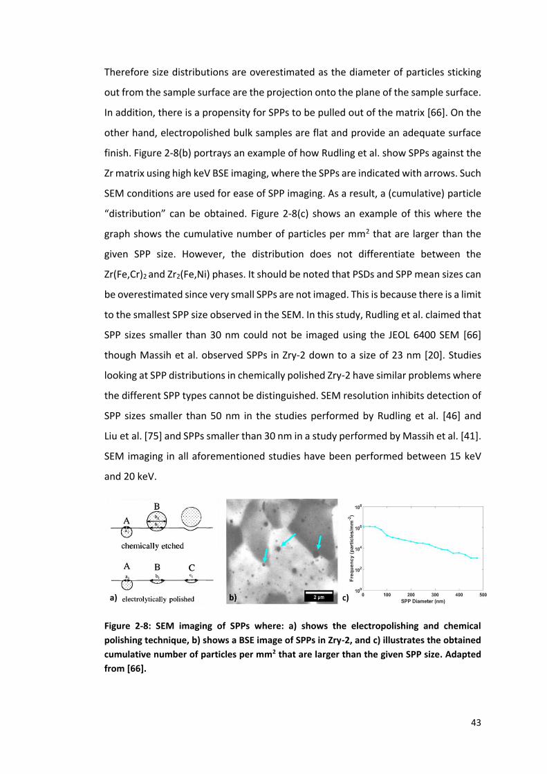
43

Therefore size distributions are overestimated as the diameter of particles sticking

out from the sample surface are the projection onto the plane of the sample surface.

In addition, there is a propensity for SPPs to be pulled out of the matrix [66]. On the

other hand, electropolished bulk samples are flat and provide an adequate surface

finish. Figure 2-8(b) portrays an example of how Rudling et al. show SPPs against the

Zr matrix using high keV BSE imaging, where the SPPs are indicated with arrows. Such

SEM conditions are used for ease of SPP imaging. As a result, a (cumulative) particle

“distribution” can be obtained. Figure 2-8(c) shows an example of this where the

graph shows the cumulative number of particles per mm2 that are larger than the

given SPP size. However, the distribution does not differentiate between the

Zr(Fe,Cr)2 and Zr2(Fe,Ni) phases. It should be noted that PSDs and SPP mean sizes can

be overestimated since very small SPPs are not imaged. This is because there is a limit

to the smallest SPP size observed in the SEM. In this study, Rudling et al. claimed that

SPP sizes smaller than 30 nm could not be imaged using the JEOL 6400 SEM [66]

though Massih et al. observed SPPs in Zry-2 down to a size of 23 nm [20]. Studies

looking at SPP distributions in chemically polished Zry-2 have similar problems where

the different SPP types cannot be distinguished. SEM resolution inhibits detection of

SPP sizes smaller than 50 nm in the studies performed by Rudling et al. [46] and

Liu et al. [75] and SPPs smaller than 30 nm in a study performed by Massih et al. [41].

SEM imaging in all aforementioned studies have been performed between 15 keV

and 20 keV.

Figure 2-8: SEM imaging of SPPs where: a) shows the electropolishing and chemical

polishing technique, b) shows a BSE image of SPPs in Zry-2, and c) illustrates the obtained

cumulative number of particles per mm2 that are larger than the given SPP size. Adapted

from [66].

44

2.4.2 (Scanning) Transmission Electron Microscopy

SEM characterization of SPPs is not as readily performed as transmission electron

microscopy (TEM) or scanning-TEM (STEM) characterization. SEM characterization

does not capture the presence of very small SPPs due to its limited resolution [46].

(S)TEM can achieve higher resolution with higher accelerating voltages and reducing

the sample thickness to 100 nm. This thickness is obtained mainly from twinjet

electropolishing of the TEM foils from an initial thickness of approximately 100 μm.

It should be noted that thinner specimens can be obtained from focussed ion beam

(FIB) milling of specific regions of interest in the material.

Specimens examined in (S)TEM are limited to the size of approximately 3 mm. With

the small thickness, feature characterization over a spatial range from the atomic

scale through to the micrometre scale can be achieved [76]. SPP counts can vary

depending on the SPP size imaged. Figure 2-9 illustrates this from a study performed

by Kruger et al. using STEM on Zry-2 specimens subject to different

thermomechanical processes [17]. The “as-received”, in Figure 2-9(a), sample only

has 84 SPPs imaged with a larger mean size. Specimen “B+1”, in Figure 2-9(b), has

357 SPPs imaged since they are smaller and more frequent despite the small image

area. However, in the majority of material treatments, there is a limit to SPP counts

and total area that can be imaged. For instance, Garzarolli et al. used TEM to study

SPPs in Zry-2 and Zry-4 where measurements were performed in an area of

200 µm2 [44]. Nevertheless, as with SEM imaging, SPP analysis in (S)TEM is a direct

method since SPP sizes can be measured, leading to SPP characteristics such as mean

size and number density being determined. Global quantities such as SPP volume

fraction can also be determined. Another difference between SEM and TEM is that

the latter has the capability of using electron diffraction to determine crystal

structures. In addition, STEM specifically allows for more accurate chemical

identification of features down to the atomic scale [76]. However, as with the SEM,

mean matrix chemistries are not reliably determined using chemical analysis due to

the large contribution that the matrix can have to the signals. The benefits of the

higher resolution are balanced by the time required for SPP analysis. Unlike SPP

analysis using SEM, (S)TEM analysis requires more time for sample preparation,

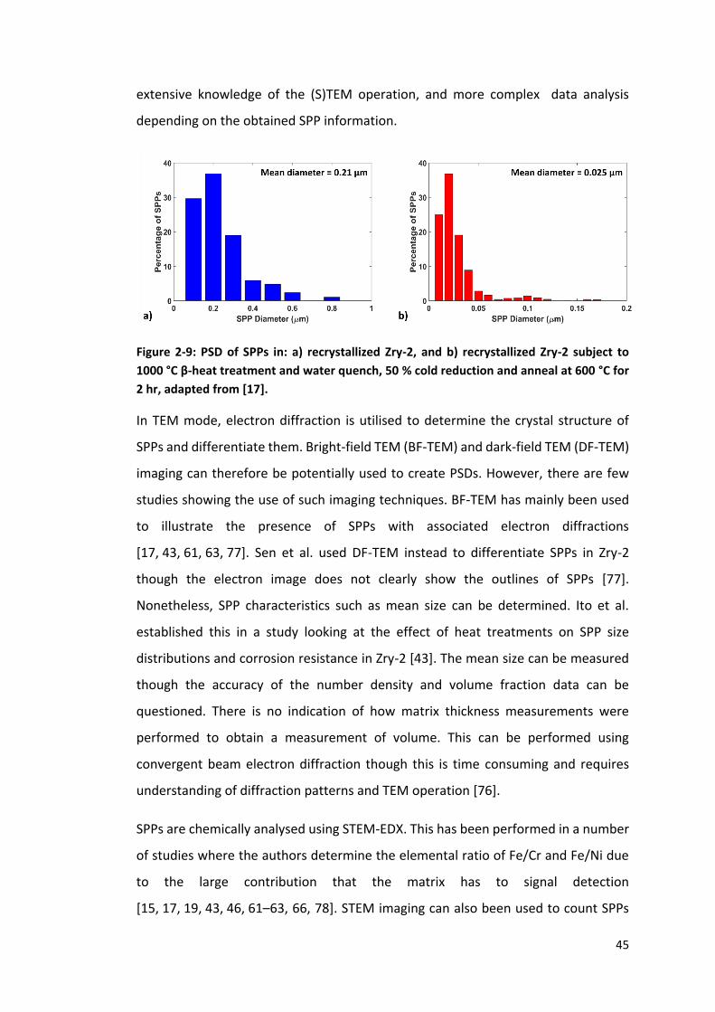
45

extensive knowledge of the (S)TEM operation, and more complex data analysis

depending on the obtained SPP information.

Figure 2-9: PSD of SPPs in: a) recrystallized Zry-2, and b) recrystallized Zry-2 subject to

1000 °C β-heat treatment and water quench, 50 % cold reduction and anneal at 600 °C for

2 hr, adapted from [17].

In TEM mode, electron diffraction is utilised to determine the crystal structure of

SPPs and differentiate them. Bright-field TEM (BF-TEM) and dark-field TEM (DF-TEM)

imaging can therefore be potentially used to create PSDs. However, there are few

studies showing the use of such imaging techniques. BF-TEM has mainly been used

to illustrate the presence of SPPs with associated electron diffractions

[17, 43, 61, 63, 77]. Sen et al. used DF-TEM instead to differentiate SPPs in Zry-2

though the electron image does not clearly show the outlines of SPPs [77].

Nonetheless, SPP characteristics such as mean size can be determined. Ito et al.

established this in a study looking at the effect of heat treatments on SPP size

distributions and corrosion resistance in Zry-2 [43]. The mean size can be measured

though the accuracy of the number density and volume fraction data can be

questioned. There is no indication of how matrix thickness measurements were

performed to obtain a measurement of volume. This can be performed using

convergent beam electron diffraction though this is time consuming and requires

understanding of diffraction patterns and TEM operation [76].

SPPs are chemically analysed using STEM-EDX. This has been performed in a number

of studies where the authors determine the elemental ratio of Fe/Cr and Fe/Ni due

to the large contribution that the matrix has to signal detection

[15, 17, 19, 43, 46, 61–63, 66, 78]. STEM imaging can also been used to count SPPs

46

though PSDs obtained using this technique do not separate the individual

contributions that the SPP types have on the distribution.

2.4.3 Atom Probe Tomography

Atom probe tomography (APT) is performed on needle shaped specimens, with

specific features such as SPPs, grain boundaries etc., with a sharp tip in the order of

10’s nm and a length of less than 1 µm. This is produced initially with electropolishing

before a lift-out with FIB milling is performed [79]. This technique identifies elements

as a function of position. As a result of this, the distribution of alloying elements in

the matrix and along grain boundaries can be determined [80–83]. For example,

Kruger et al. utilised APT to show trends in nodular corrosion resistance with matrix

solute content and SPP size distribution where the optimum performance is obtained

with small SPPs and high solute concentration in the matrix [17]. SPPs can be

observed within the needle though their size is limited. Figure 2-10 illustrates how

the sample geometry limitation affects SPP sizes where they are less than 50 nm. As

with (S)TEM analysis, SPP counts are dependent on their size in the needle.

Sundell et al. showed that there is a high number density of SPPs, mainly Zr(Fe,Cr)2

with sizes less than 5 nm, in Zry-2 after 9 cycles of in-reactor exposure [82]. It should

be noted that the resolution of APT is approximately 1 nm [84]. Then again, if the

SPPs are larger, then there is a lower SPP count. Nonetheless, SPP sizes, number

density, and volume fraction can be evaluated though these will not be

representative of those observed in bulk materials. SPP chemistry can also be

determined by counting ions in the clusters though the SPP crystal structures cannot

be determined using APT. APT is considered to be a slow technique for SPP analysis

since the needle preparation needs to be extremely accurate.

47

Figure 2-10: APT reconstruction of irradiation-induced precipitates with Fe and Cr, adapted

from [67].

2.4.4 Differential Scanning Calorimetry

Differential scanning calorimetry (DSC) is a technique that measures the difference

in heat flux between a sample and a reference, in the same furnace, while the

temperature changes. This determines the change in energy involved in phase

transformations in metals such as the dissolution or formation of SPPs.

DSC samples are limited to the size of the crucible that they are placed in. Sample

volumes are not stated in literature though sample masses are measured given that

the DSC outputs are measured in μV/mg. Sample masses range from

10 – 130 mg [85–88]. SPPs cannot be counted using this technique and as a result,

the number density, and SPP size cannot be directly determined. Further, SPPs are

not identified or chemically analysed and the mean matrix chemistry cannot be

determined using DSC. However, the evolution in SPP volume fraction can be

estimated indirectly by considering the magnitude of the enthalpy peaks when SPPs

dissolve into the matrix for different specimens subject to different heat treatments.

Transformation enthalpies are determined by calculating the area under the curves.

These curves will have varying transformation enthalpies depending on the quantity

of precipitates present in the system. In addition, the phase transformation

temperatures can be determined. Toffolon-Masclet et al. presented this by

performing high temperature, high sensitivity DSC measurements and

complementary STEM analysis on Zr-Nb alloys to show the correlations between the

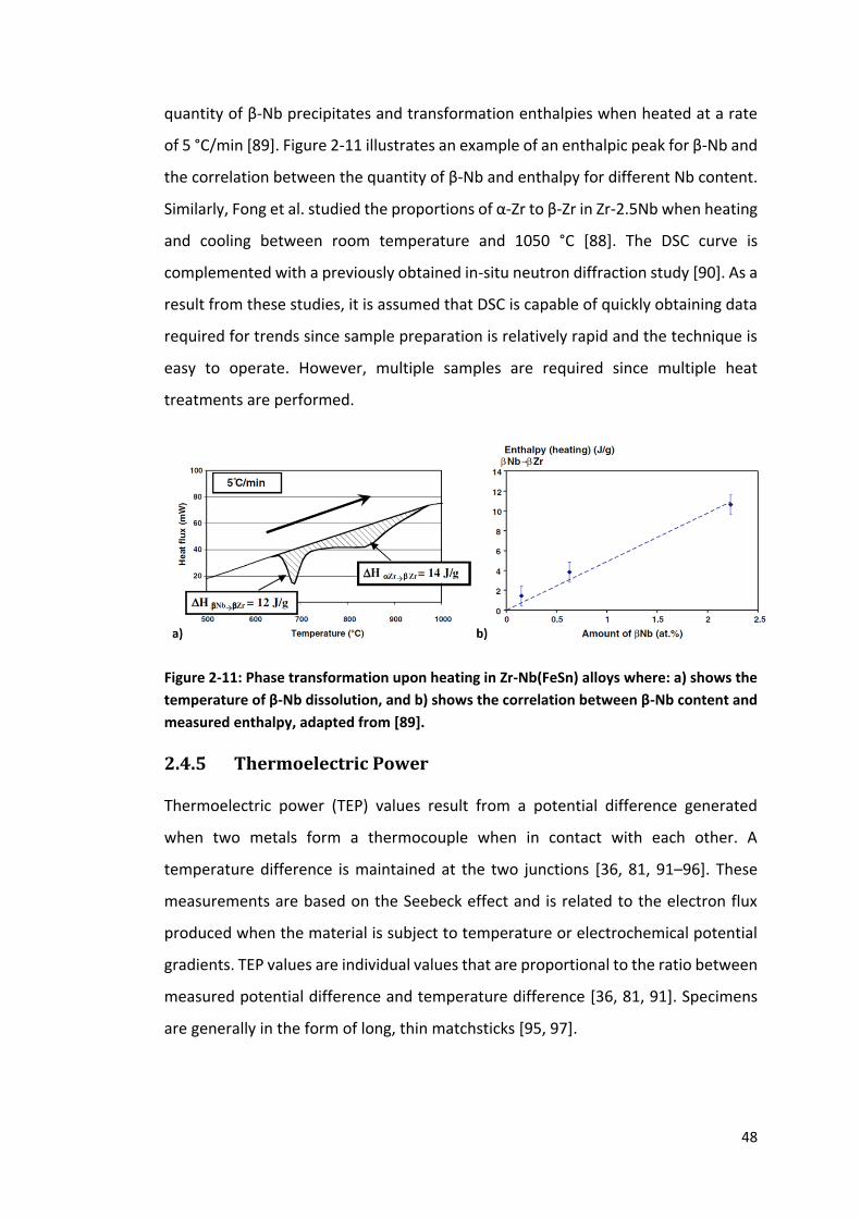
48

quantity of β-Nb precipitates and transformation enthalpies when heated at a rate

of 5 °C/min [89]. Figure 2-11 illustrates an example of an enthalpic peak for β-Nb and

the correlation between the quantity of β-Nb and enthalpy for different Nb content.

Similarly, Fong et al. studied the proportions of α-Zr to β-Zr in Zr-2.5Nb when heating

and cooling between room temperature and 1050 °C [88]. The DSC curve is

complemented with a previously obtained in-situ neutron diffraction study [90]. As a

result from these studies, it is assumed that DSC is capable of quickly obtaining data

required for trends since sample preparation is relatively rapid and the technique is

easy to operate. However, multiple samples are required since multiple heat

treatments are performed.

Figure 2-11: Phase transformation upon heating in Zr-Nb(FeSn) alloys where: a) shows the

temperature of β-Nb dissolution, and b) shows the correlation between β-Nb content and

measured enthalpy, adapted from [89].

2.4.5 Thermoelectric Power

Thermoelectric power (TEP) values result from a potential difference generated

when two metals form a thermocouple when in contact with each other. A

temperature difference is maintained at the two junctions [36, 81, 91–96]. These

measurements are based on the Seebeck effect and is related to the electron flux

produced when the material is subject to temperature or electrochemical potential

gradients. TEP values are individual values that are proportional to the ratio between

measured potential difference and temperature difference [36, 81, 91]. Specimens

are generally in the form of long, thin matchsticks [95, 97].

49

TEP is sensitive to a material’s microstructure including the presence of

imperfections, and alloying elements in solution. Variations in TEP is affected by

processing parameters such as cold work, and heat treatment temperature and

time [98]. TEP measurements have thus far mainly been performed at ambient

temperature since sensitivity of TEP to materials is high [95, 97]. Since the TEP values

are dependent on the presence features such as defects and impurity/solute atoms,

and provides an individual value, this technique does not provide information

regarding SPP characteristics such as mean size, number density, and volume

fraction. In addition, SPP chemistry and crystal structure cannot be identified.

Instead, TEP has the capability of measuring the extent of the solute concentration

in the matrix. The valence electrons in solute atoms occupy the hybridized d-level

orbitals of the solvent atoms, leading to a more negative TEP than that for the solvent

on its own [91]. In addition, if solute atoms have fewer available d-orbitals than that

for the solvent, the TEP becomes more negative. In the case of Zry-2 and HiFi, the

solute elements of Fe, Cr, and Ni have fewer available d-orbitals than Zr. This means

the addition of these solute atoms decreases the TEP. The greater the solute content,

the more negative the TEP value. When precipitation occurs, the concentration of

solutes reduces and the TEP value to be more positive [99]. Figure 2-12 provides an

example for this where α-quenched Zry-2 is heat-treated at 450 °C – 600 °C for

different lengths of time [94]. The plateau in TEP value at longer heat treatment

times, especially seen at 600 °C, suggests that the solute concentration in the matrix

is constant and the precipitation process is complete. From this, TEP data is quick to

obtain since sample preparation is quick and a single data point is obtained for each

sample. Though as with DSC, multiple samples are required since multiple heat

treatments are usually performed in order to identify trends.

50

Figure 2-12: TEP evolution in α-quenched Zry-2 is heat-treated at 450 °C – 600 °C with

varying times, adapted from [94].

2.4.6 X-ray Diffraction

With X-ray diffraction (XRD), large samples, centimetres in size, can be used to

identify the crystal structure of SPPs in the matrix. The larger the sample, the greater

the peak intensity at particular d-spacings. Synchrotron XRD is usually used for SPP

analysis since laboratory XRD has a lower energy source and thus has insufficient

resolution to differentiate SPP peaks [36]. SPPs cannot be counted using this

technique and therefore the number density cannot be determined. The SPP volume

fraction also cannot be determined directly using XRD though it could be tracked.

With further heat treatments, the SPP peaks sharpen and new peaks form,

corresponding to the formation of new SPPs. Motta et al. and Erwin et al. illustrated

this in their studies of synchrotron radiation on SPPs in Zr alloys where, looking at

Zry-2 and Zry-4, the authors performed a number of heat treatments on β-quenched

material [49, 100]. Figure 2-13 illustrates the diffraction pattern obtained for Zry-2

with a cumulative annealing parameter (𝛸CAP) of 1 × 10−16 hr. Towards this high

CAP value, the intensity peaks seem to be reaching a constant intensity. Though it

should be noted that a high temperature / low time combination (815 °C / 1 hr) has

been used to model 𝛸CAP where different temperature/time combinations for the

same 𝛸CAP values change SPP size distributions [42–44, 50, 80, 101, 102]. As seen

from Figure 2-13, SPPs can be identified from the diffraction patterns obtained

51

though the SPP chemistry – for instance the ratio of solutes in the SPPs – cannot be

established.

Figure 2-13: Synchrotron radiation diffraction pattern of Zry-2 with 𝜲𝐂𝐀𝐏 of 𝟏 × 𝟏𝟎−𝟏𝟔 hr,

adapted from [49].

Synchrotron XRD can also be used to measure the mean concentration of solutes in

the matrix. This is accomplished by measuring the change in lattice parameter in the

matrix. Ivermark et al. showed this by performing a study on deformed or un-

deformed Nb-containing Zr alloys which were subsequently heat-treated. This is

identified by the slight shifts in the α-Zr and β-Zr intensity peaks with further heat-

treatments [103].

Small angle x-ray scattering (SAXS) is another technique available at synchrotrons. It

is capable of identifying the shape and size distribution of SPPs in Zr alloys though it

is not used as readily as synchrotron XRD. One of the drawbacks to this technique is

the limited sample geometry where the sample has to be chemically polished in a

solution of nitric acid and hydrofluoric acid to be 15-25 µm thick [77, 104].

Nonetheless, Sen et al. used SAXS it investigate the evolution of SPPs in stress-

relieved Zry-2, and β-quenched Zry-2 which was subsequently heat treated at

550 °C [77]. The authors were able to track the increase in SPP size with increased

ageing though SPPs larger than 200 nm could not be observed due to instrument

52

limitations where 𝑞 range in reciprocal space was limited (where 𝑞 is the scattering

vector magnitude). Alternatively, ultra-small angle x-ray scattering (USAXS) can be

used to provide information on precipitates in the size range of 10 nm to 2 µm. USAXS

has a better 𝑞 resolution than SAXS, leading to much larger sample sizes

(approximately 100 µm thick) and larger SPP counts. Srirangum et al. performed

USAXS on Zry-4 that was β-quenched and then heat treated at 600 °C to illustrate

how this affects the evolution of Zr(Fe,Cr)2 particles [105]. The authors clearly

demonstrated that with increased ageing, the PSD broadens, and the volume fraction

and number density both increase. However, the different SPP types cannot be

distinguished using either SAXS or USAXS though complimentary TEM or STEM-EDX

experimental work can account for this. In addition, SPP chemistry and the matrix

chemistry cannot be measured using (U)SAXS.

2.5 Effect of Processing on SPPs in Zr Cladding

2.5.1 β-Quenching

Water quenching from a solution heat treatment in the β-Zr phase (≥ 1050 °C) to

room temperature can have cooling rates up to 1500 °C/s [36, 37, 105]. The phase

transformation from β-Zr to α-Zr leads to the formation of α-Zr laths accompanied

with dislocations within the lath and SPPs along the lath boundaries [14, 37, 68]. A

number of studies on β-quenched Zry-4 have observed SPP sizes ranging from 10 nm

to 100 nm [37, 104, 105] while Massih et al. observed SPPs in Zry-2 within the size

range of 20 nm to 500 nm with a high number density of SPPs less than 50 nm in

size [41]. Jeong et al. demonstrated that quenching rates up to 2100 °C/s can be

obtained by quenching in an ice-brine solution. From TEM imaging, the formation of

SPPs seem to be prohibited (since the authors do not present SPP sizes or volume

fraction data for this particular process) and thus the matrix is supersaturated in

solutes [37]. However, this could result from the fact that the SPP sizes following

quenching in an ice-brine solution are lower than the TEM’s resolution limit. Slower

cooling rates are achieved by cooling in oil, air, or the furnace with cooling rates

approximately of 110, 4, and 0.1 °C/s [37]. This leads to larger α-Zr laths and generally

small number density of larger SPPs, and a larger SPP volume fraction [20, 37, 41].

53

2.5.2 Hot Extrusion

Hot extrusion involves preheating the material before the extrusion process. Hot

rolling is used to simulate hot extrusion by examining plates instead of tubes. Liu et

al. performed hot rolling, with approximately 60 % reduction, with pre-heat

temperatures ranging from 750 °C to 820 °C on Zr-Sn-Nb-Fe-Cr plates [106]. The

750 °C hot roll showed homogenous SPP distribution though higher temperature

rolls led to SPP agglomeration since β-Zr is formed and retains solutes which then

precipitated out on cooling or further annealing. On the other hand, Chen et al.

performed different studies on hot rolling of β-quenched Zr-Sn-Nb-Fe-Cu-O-(Si) with

a maximum reduction of 75 % with a pre-heat at 480 °C and 600 °C. SPPs are mainly

found along grain boundaries, similar to that seen after β-quenching, though there is

slight distortion to the microstructure with increased percentage reduction [68, 69].

Limited SPP growth is observed in both studies though the SPP size is larger when the

pre-heat is at 600 °C, where the average size is approximately 50 nm, than that at

480 °C where the average SPP size is 30 nm.

2.5.3 Cold Pilgering

Cold pilgering reduces the inner radius and thickness of tubes at room temperature.

Cold pilgering with a high enough deformation can change the spatial distribution of

SPPs present from previous β-quenching or extrusion processes. Qiu et al.

demonstrated this with reductions up to 50 % on Zr-1.0Sn-1.0Nb-0.12Fe tube

material where this is thought to result from the radial and tangential compression

that the tube is subject to during the pilgering process [70]. In addition, it was

observed that with increased deformation, the mean SPP size reduces very slightly

despite the SPP volume fraction staying constant, suggesting that precipitation took

place prior to the cold pilger process. In contrast, Garzarolli et al. discovered that the

mean SPP size of Zry-2 and Zry-4 cladding tubes, from different processing routes, is

unaffected by the accumulation of cold-work steps [44]. Though it should be noted

that the SPP mean size was obtained when examining the final product.

54

2.5.4 Heat Treatments

SPPs increase in size when both the annealing temperature and annealing time

increases. The SPP size distribution also widens and shifts to larger sizes with the

spread becoming less skewed with further heat treatments. Kruger et al.

demonstrated this when comparing SPP sizes on as-received Zry-2 tubing and that

subject to a heat treatment of 800 °C / 1 hr [17]. Here, the median SPP size increases

slightly with the heat treatment while the number density of SPPs smaller than

200 nm decreases. Luan et al. also demonstrates this on β-quenched Zr-0.85Sn-

0.4Nb-0.1Cr-0.05Cu subject to heat treatments at 600-700 °C for 0.5-30 hr [72].

Increasing the annealing time, for the same annealing temperature, leads to an

increase in SPP mean size. The same is observed when increasing annealing

temperature at a constant annealing time (Figure 2-14) though the SPP distribution

is much broader at the higher temperature. This illustrates the profound effect that

temperature has on SPP growth. Nonetheless, the SPP volume fraction was found to

be relatively constant at 2.10 ± 0.05 % for all heat treatments, suggesting that all SPPs

have precipitated out. Gros and Wadier observed a similar effect on SPPs in Zry-4

when subject to heat treatments at 650-780 °C for 0.5-30 hr [107].

Figure 2-14: PSD of Zr-0.85Sn-0.4Nb-0.1Cr-0.05Cu alloy annealed at 600 °C / 0.5 hr,

650 °C / 30 hr, and 700 °C / 30 hr, adapted from [72].

Heat treatments during manufacturing can be interpreted by the annealing

parameter, 𝛸A. Equation 2-1 illustrates this where Steinburg et al. correlated the final

55

annealing temperature and final annealing time to the material’s yield strength in

recrystallized Zry-4 tubes [108]:

𝛸A = 𝑡 exp [−𝑄

𝑅𝑇] (2-1)

where 𝑡 is the annealing time, 𝑇 is the annealing temperature, 𝑄 is the activation

energy for recrystallization in Zry-4, and 𝑅 is the molar gas constant. Equation 2-1 is

an exponential (Arrhenius) relationship since it empirically correlated the annealing

time and temperature to the yield strength of recrystallized Zry-4 [108].

Andersson et al. accounted for the contribution that intermediate heat treatments

have, following the last β-quench, by defining the cumulative annealing parameter,

𝛸CAP [48]:

𝛸CAP = ∑ 𝑡𝑖 exp [−𝑄

𝑅𝑇𝑖]𝑖

1 (2-2)

where 𝑖 represents the accumulation of different heat treatments. The value of the

activation energy, 𝑄, is the average of the activation energies from different

combinations of annealing time and temperature, and oxide weight gain on Zry-4

tubing. 𝛸CAP is in the form shown in Equation 2-2 since Andersson et al. assumed

that Zry-4 corrosion properties are controlled by thermal processes such as diffusion

of alloying elements [48]. It should be noted that the authors used 𝛸CAP to describe

corrosion properties of Zry-4 tubing without coupling to material properties such as

SPP size and solute concentration. Nonetheless, many studies have established

correlations between 𝛸CAP and mean SPP size where the mean SPP size increases

with increased 𝛸CAP [42–44, 50, 80, 101, 102]. As a result, SPP distributions widen

and shift to larger sizes. Figure 2-15(a) depicts an example of this where Anada et al.

demonstrated the effect of varying 𝛸CAP on sheet Zry-4 [101]. There is a high number

density of SPPs that are smaller than 200 nm in size when the 𝛸CAP is 8.2 × 10−19 hr

and this decreases with increased 𝛸CAP. This leads to a distribution that is less skewed

to smaller SPP sizes. In addition, quantities of SPPs in certain size ranges evolve with

𝛸CAP. Figure 2-15(b) shows this where the “< 100 nm” range decreases in SPP

frequency with increased 𝛸CAP while the SPP frequency of the “> 300 nm” range

increases. The frequency of the “200-300 nm” range increases more rapidly than the

“> 300 nm” range due to the rapid ripening of SPPs smaller than 200 nm.

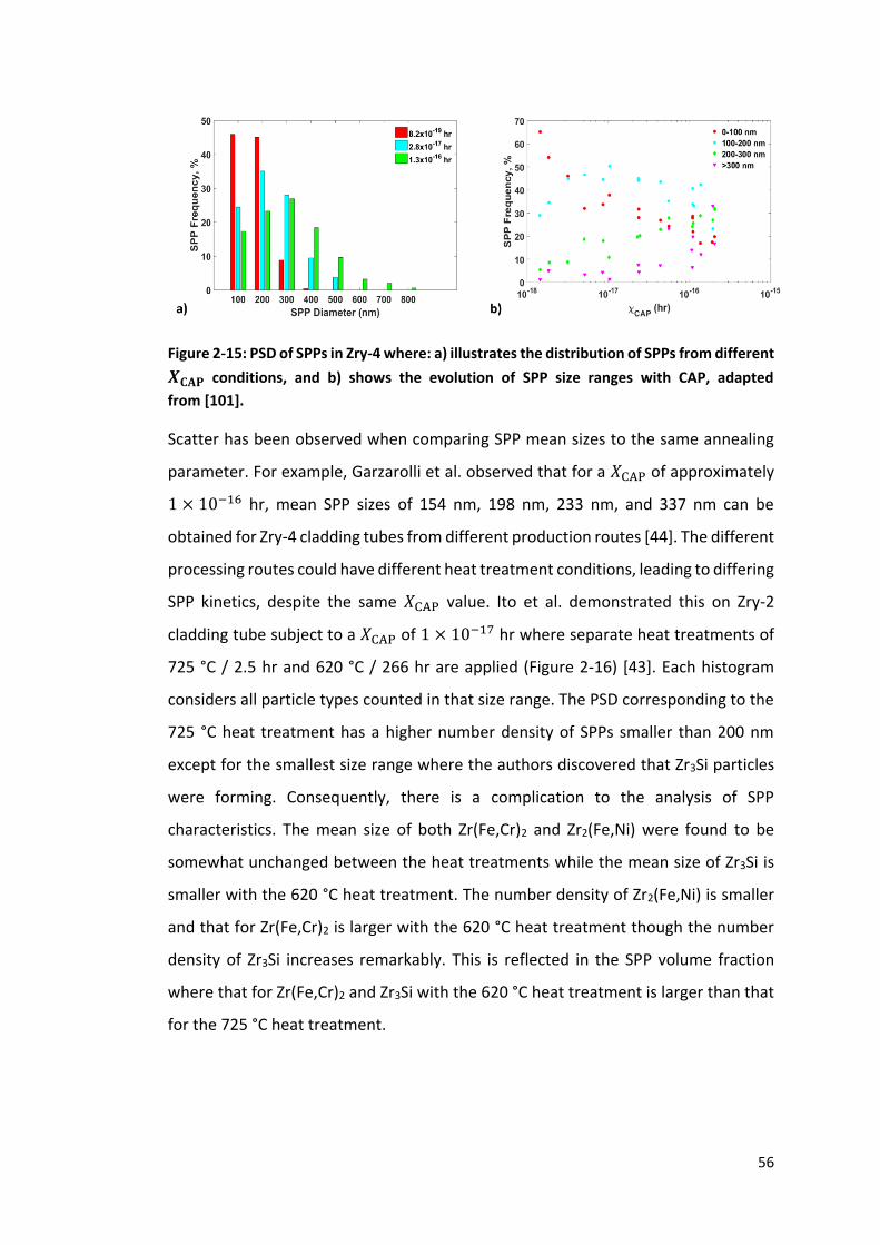
56

Figure 2-15: PSD of SPPs in Zry-4 where: a) illustrates the distribution of SPPs from different

𝜲𝐂𝐀𝐏 conditions, and b) shows the evolution of SPP size ranges with CAP, adapted

from [101].

Scatter has been observed when comparing SPP mean sizes to the same annealing

parameter. For example, Garzarolli et al. observed that for a 𝛸CAP of approximately

1 × 10−16 hr, mean SPP sizes of 154 nm, 198 nm, 233 nm, and 337 nm can be

obtained for Zry-4 cladding tubes from different production routes [44]. The different

processing routes could have different heat treatment conditions, leading to differing

SPP kinetics, despite the same 𝛸CAP value. Ito et al. demonstrated this on Zry-2

cladding tube subject to a 𝛸CAP of 1 × 10−17 hr where separate heat treatments of

725 °C / 2.5 hr and 620 °C / 266 hr are applied (Figure 2-16) [43]. Each histogram

considers all particle types counted in that size range. The PSD corresponding to the

725 °C heat treatment has a higher number density of SPPs smaller than 200 nm

except for the smallest size range where the authors discovered that Zr3Si particles

were forming. Consequently, there is a complication to the analysis of SPP

characteristics. The mean size of both Zr(Fe,Cr)2 and Zr2(Fe,Ni) were found to be

somewhat unchanged between the heat treatments while the mean size of Zr3Si is

smaller with the 620 °C heat treatment. The number density of Zr2(Fe,Ni) is smaller

and that for Zr(Fe,Cr)2 is larger with the 620 °C heat treatment though the number

density of Zr3Si increases remarkably. This is reflected in the SPP volume fraction

where that for Zr(Fe,Cr)2 and Zr3Si with the 620 °C heat treatment is larger than that

for the 725 °C heat treatment.

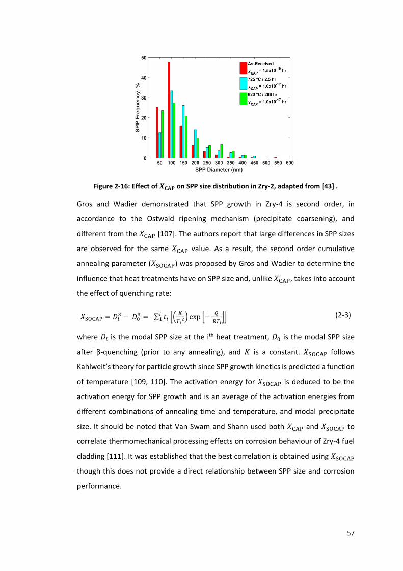
57

Figure 2-16: Effect of 𝜲𝐂𝐀𝐏 on SPP size distribution in Zry-2, adapted from [43] .

Gros and Wadier demonstrated that SPP growth in Zry-4 is second order, in

accordance to the Ostwald ripening mechanism (precipitate coarsening), and

different from the 𝛸CAP [107]. The authors report that large differences in SPP sizes

are observed for the same 𝛸CAP value. As a result, the second order cumulative

annealing parameter (𝛸SOCAP) was proposed by Gros and Wadier to determine the

influence that heat treatments have on SPP size and, unlike 𝛸CAP, takes into account

the effect of quenching rate:

𝛸SOCAP = 𝐷𝑖3 − 𝐷0

3 = ∑ 𝑡𝑖 [(𝐾

𝑇𝑖2) exp [−

𝑄

𝑅𝑇𝑖]]𝑖

1 (2-3)

where 𝐷𝑖 is the modal SPP size at the ith heat treatment, 𝐷0 is the modal SPP size

after β-quenching (prior to any annealing), and 𝐾 is a constant. 𝛸SOCAP follows

Kahlweit’s theory for particle growth since SPP growth kinetics is predicted a function

of temperature [109, 110]. The activation energy for 𝛸SOCAP is deduced to be the

activation energy for SPP growth and is an average of the activation energies from

different combinations of annealing time and temperature, and modal precipitate

size. It should be noted that Van Swam and Shann used both 𝛸CAP and 𝛸SOCAP to

correlate thermomechanical processing effects on corrosion behaviour of Zry-4 fuel

cladding [111]. It was established that the best correlation is obtained using 𝛸SOCAP

though this does not provide a direct relationship between SPP size and corrosion

performance.

58

2.5.5 The Role of SPPs in Reactor Conditions

2.5.5.1 Corrosion

Corrosion in Zr alloys is observed through the formation of ZrO2 on the surface. There

are two different types of corrosion that can be present: nodular corrosion and

uniform corrosion. Nodular corrosion is shown in the form of white nodules on the

Zr alloy surface. Uniform corrosion is seen as an even thickness layer of

oxide [112, 113].

SPPs are thought to affect the corrosion resistance of Zr alloys. This is thought to be

due to galvanic coupling between the Zr matrix and the SPPs in the alloy, limiting the

oxidation of SPPs [114]. Zry-2 cladding tubes with a high number density of small

particles (less than 100 nm in size) are thought to minimise nodular

corrosion [14, 15]. Studies also show that the solute concentration in the matrix

contributes to nodular corrosion resistance with the optimal nodular corrosion

resistance being attained with small precipitates and high solute concentration in the

matrix. Here, it is thought that local areas in the matrix that are low solute

concentration levels can be potential nucleation sites for nodules [16–19]. The

relevant size distributions can be attained by implementing a β-quench close to the

end of the processing route [14, 15, 18]. On the other hand, optimal uniform

corrosion resistance is believed to be achieved due to the presence of large SPPs

(greater than 100 nm in size) with a low number density and when solute

concentration in the matrix is at an equilibrium value. A slow β-quench rate and 𝛸CAP

values larger than 1 × 10−18 hr ensure that such conditions are met [20, 21].

2.5.5.2 Irradiation

SPPs transform from a crystalline state to an amorphous state when irradiated. This

amorphous region is correlated by a diffraction pattern with a “halo ring” and a

depletion of Fe [115, 116]. It should be noted that new SPPs can also form as a result

of irradiation. Fe- or Cr-rich nano-rods or clusters (≤ 150 nm) have been observed in

neutron and proton irradiated Zry-2 using STEM-EDX and atom probe tomography.

These small SPPs could have formed due to the driving force for re-precipitation

counteracting the randomised distribution of solutes caused by irradiation and the

59

low solubility limit of Fe and Cr in α-Zr [82, 117, 118]. This has the effect of shifting

the PSD to smaller sizes and thus improving corrosion resistance [119, 120].

However, it is unclear whether the re-precipitation is caused by irradiation itself or

by post-irradiation cooling.

2.6 Second Phase Particle Precipitation in the Solid State

SPP precipitation kinetics in Zr alloys is of importance since SPPs evolve throughout

the stages in thermomechanical processing. This is separated into separate regimes:

nucleation, growth, and coarsening.

2.6.1 SPP Nucleation

Phase transformations of interest are thermally activated, leading to change from

the single phase region of the phase diagram to the region where multiple phases

are stable. Precipitation, illustrated in Figure 2-17, can be expressed as:

𝛽 → 𝛼 + 𝜑 (2-4)

where 𝛽 is the single phase, 𝛼 is the metastable supersaturated solid solution, and 𝜑

is the precipitate. Nucleation of the precipitate in the solid state can either be

homogeneous or heterogeneous.

Figure 2-17: Precipitation phase transformation in simple binary alloy where: β is the single

phase, α is the metastable supersaturated solid solution, ϕ is the precipitate, T is

temperature and cB is the concentration of the “B” phase. Adapted from [121].

60

2.6.1.1 Homogeneous Nucleation

Homogeneous nucleation takes place with equal probability without there being a

bias towards a specific location. Precipitation of a secondary phase from a

supersaturated solid solution requires a number of atoms diffusing together to form

a small cluster. This transformation leads to a change in free energy. The chemical

driving force of the system reduces when the cluster forms. In addition, an interface

between the cluster and matrix is formed, providing a positive contribution to the

free energy change. Further, a misfit strain energy is present since the new phase will

not perfectly match the matrix lattice, another positive contribution to the free

energy. Equation 2-5 expresses the aforementioned changes to the free energy for

homogeneous nucleation of precipitates, ∆𝐺hom [121]:

∆𝐺hom = −𝑉φ(∆𝐺V − ∆𝐺s) + 𝐴𝛾 (2-5)

where 𝑉φ is the volume of the 𝛾 precipitate, ∆𝐺V is the change in free energy per unit

volume between the 𝛽 and 𝛼 phases (where ∆𝐺V = ∆𝐺Vβ

− ∆𝐺Vα), ∆𝐺s is the strain

energy per unit volume between the different phases, 𝐴 is the area of the interface

between the 𝛽 and 𝛼 phases, and 𝛾 is the interfacial energy. It should be noted that

the value of the interfacial energy depends on the nature of the particle interface.

This ranges between 0.1 J/m2 (coherent interface) and 1 J/m2 (incoherent interface).

The strain energy is also affected by interface type where coherent interfaces have a

higher strain energy and incoherent interfaces have a lower strain energy [122, 123].

Assuming the precipitate is spherical, ∆𝐺hom can be expressed as [121, 123]:

∆𝐺hom = −4

3𝜋𝑟3(∆𝐺V − ∆𝐺s) + 4𝜋𝑟2𝛾 (2-6)

Figure 2-18 demonstrates the contribution of the terms in Equation 2-6 where the

strain energy term reduces the transformation’s effective driving force.

61

Figure 2-18: Gibbs free energy as a function of particle size for solid phase precipitation,

adapted from [121].

There is a critical radius, 𝑟∗, shown in Figure 2-18, where the change in free energy is

at its maximum. If a cluster forms with a radius less than 𝑟∗, free energy has to be

inputted into the system in order to overcome this activation energy. The cluster is

therefore unstable and thus dissolves into the solid solution. Conversely, if a cluster

is larger than 𝑟∗, the system is able to reduce its free energy whilst the cluster grows.

𝑟∗ is determined by differentiating Equation 2-6. In turn, the critical free energy, ∆𝐺∗,

is established:

𝑟∗ = 2𝛾

(∆𝐺V−∆𝐺s) (2-7)

∆𝐺hom∗ =

16𝜋𝛾3

3(∆𝐺V−∆𝐺s)2 (2-8)

The nucleation rate of nuclei, 𝐽hom, with a critical size is defined in Equation 2-9.

𝐽hom = 𝐶0𝑍𝑓 exp [−(∆𝐺hom

∗ )

𝑘𝑇] (2-9)

where 𝐶0 is the number of homogeneous nucleation sites per unit volume, where

each atom represents a potential site for nucleation, 𝑍 is the dimensionless Zeldovich

factor (considers the probability of continued growth of thermally activated critically

sized clusters), 𝑓 is the rate of attachment of a solute atom to the nucleus, 𝑘 is the

Boltzmann constant, and 𝑇 is the temperature [123, 124].

It should be noted that homogeneous nucleation is not usually seen in real materials

with the exception of Cu-Co binary alloys with Co concentrations ranging from

62

0.5 at% to 2.7 at%. The 2 % difference in lattice parameter between Cu and Co (both

face-centred cubic crystal structures) leads to minimal coherency strain when Co

particles are formed [121, 125–127].

2.6.1.2 Heterogeneous Nucleation

Heterogeneous nucleation in the solid state takes place on defects such as vacancies,

dislocations, grain boundaries, and inclusions [121, 123]. These nucleation sites

increase the system’s free energy. Therefore, if a cluster forms on a defect and

destroys it, some free energy is released from the system and the activation energy

barrier reduces. The free energy for heterogeneous nucleation, ∆𝐺het, is expressed

in Equation 2-10 [121]:

∆𝐺het = −𝑉φ(∆𝐺V − ∆𝐺s) + 𝐴𝛾 − ∆𝐺d (2-10)

The (critical) free energies for homogeneous and heterogeneous nucleation are

similar with the difference being that heterogeneous nucleation has the addition of

a shape factor, 𝑆(𝜃). Equation 2-11 illustrates this where 𝑆(𝜃) is dependent on the

angle between the matrix and cluster interface [121, 123]. Further, the shape factor

changes depending on the type of defect on which heterogeneous nucleation occurs

on. Equation 2-12 provides an example of the form of the shape factor for grain

boundary nucleation.

∆𝐺het∗ = ∆𝐺hom

∗ 𝑆(𝜃) (2-11)

𝑆(𝜃) = 1

2(2 + cos 𝜃)(1 − cos 𝜃)2 (2-12)

The shape factor is in the range of 0 ≤ 𝑆(𝜃) ≤ 1 since it is dependent on 𝜃 (the

shape of the nucleus). Therefore, ∆𝐺het∗ will always be smaller than ∆𝐺hom

∗ , as

illustrated in Figure 2-19.

63

Figure 2-19: Gibbs free energy for heterogeneous (∆𝑮𝐡𝐞𝐭) and homogeneous (∆𝑮𝐡𝐨𝐦)

nucleation as a function of particle size, adapted from [121].

Similarly to the homogeneous nucleation rate (Equation 2-9), the heterogeneous

nucleation rate can be expressed as [123, 124, 128]:

𝐽het = 𝐶1𝑍𝑓 exp [−(∆𝐺het

∗ )

𝑘𝑇] (2-13)

where 𝐶1 is the number of heterogeneous nucleation sites per unit volume.

2.6.2 SPP Growth

The driving force for SPP growth is the solute diffusion between the newly formed

nucleus and the supersaturated matrix. This is due to a solute concentration gradient

present around the nucleus. The growth rate is controlled in one of two ways. For

smaller particles, the rate controlling factor is the rate of atoms crossing the

particle/matrix interface. The rate controlling factor for larger particles is the

diffusion of atoms to the interface. Though it should be noted that the widely-

accepted rate controlling factor for particle growth is the diffusion of atoms to the

interface since this is adequate to obtain equilibrium at the

interface [122, 123, 128, 129]. Equation 2-14 depicts the growth rate of spherical

particles where the diffusion of atoms to the interface is the rate controlling

factor [122, 123, 128, 130–135]:

𝑣(𝑟) = 𝑑𝑟

𝑑𝑡 =

𝑐i− 𝑐r

𝑐φ− 𝑐r

𝐷

𝑟 (2-14)

64

where 𝑐i is the instantaneous solute concentration in the matrix, 𝑐φ is the solute

concentration within the particle, 𝐷 is the solute diffusion coefficient, and 𝑐r is the

solute concentration of the interface on the matrix side and . Equation 2-15 describes

the diffusion coefficient of solutes:

𝐷 = 𝐷0 exp [−𝑄

𝑅𝑇] (2-15)

where 𝐷0 is the diffusivity coefficient of solutes in the matrix. Solute diffusion is a

thermally activated process where an atom moves from one site to another. The

activation energy, 𝑄, is the energy necessary for the atom to move. Equation 2-15

describes the probability of such a motion where it depends exponentially from

temperature i.e. follows the Arrhenius dependence.

𝑐r portrays the effect that the particle’s finite radius of curvature has on the solute

concentration at the interface on the matrix side:

𝑐r = 𝑐α∞ exp [

2𝛾𝑉φm

𝑅𝑇∙

1

𝑟] (2-16)

where 𝑐α∞ is the solute concentration in the matrix when at equilibrium, 𝑉φ

m is the

molar volume of the precipitate, and 𝑅 is the gas constant. The addition of new

particles to the matrix increases the free energy of the system, and shifts it away

from equilibrium, by introducing particle interfaces. This known as the Gibbs-

Thomson effect (Figure 2-20) [122, 123, 128]. If there are two β-phase particles of

different sizes in the α-phase matrix, the smaller particle (with a smaller radius of

curvature r2) has a higher molar free energy than that for the larger particle. This is

due to the higher interfacial energy associated with the smaller particle. From

Equation 2-16, the smaller particle will therefore have a higher concentration of

solutes in the matrix adjacent to the particle. With increasing radius of curvature, the

system’s free energy and thus the solute concentration in the matrix adjacent to the

particle decreases further until an equilibrium value is reached.

65

Figure 2-20: Schematic illustrating the effect that the radius of curvature of a particle has

on the free energy (G) of the system (Gibbs-Thomson effect) and the solute concentration

in the matrix adjacent to the particle (XB). Particles with differing radii of curvature,

residing in the matrix (with a free energy, Gα), have different interfacial energies. A smaller

particle (radius of curvature, r2) has a higher interfacial energy than that for the larger

particle (radius of curvature r1). The smaller particle therefore has a larger free energy and

thus has a larger solute concentration adjacent to it in the matrix (X2) than that associated

to the larger particle (X1). Adapted from [121].

During the growth regime, the precipitates’ morphology is affected by the anisotropy

of the interfacial energy at the particle/matrix interfaces. The driving force is to

obtain minimal total interfacial energy. Precipitates usually have a combination of

interface types (coherent, semi-coherent or incoherent) that limit its shape through

interface migration at different migration rates. For example, incoherent interfaces

have a high mobility in comparison to semi-coherent interfaces, leading to disc- or

plate-shaped precipitates, as shown in Figure 2-21(a). Precipitates formed on

defects, such as grain boundaries, generally grow at larger rates since they act as

sinks for solutes. Solutes then diffuse along the grain boundary, attaching to the

precipitate before diffusing along the interfaces. Figure 2-21(b) illustrates this. This

type of growth is more common for substitutional diffusion. It should be noted that,

solute segregation to grain boundaries in Zr is possible throughout

thermomechanical processing though no studies have been performed to

demonstrate this. Instead, studies have identified that solute segregation to and

from grain boundaries takes place during neutron irradiation of Zry-2 though this was

not reviewed extensively and appears to be minimal [117].

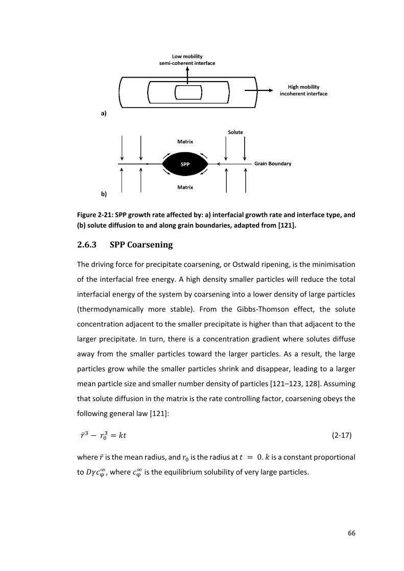
66

Figure 2-21: SPP growth rate affected by: a) interfacial growth rate and interface type, and

(b) solute diffusion to and along grain boundaries, adapted from [121].

2.6.3 SPP Coarsening

The driving force for precipitate coarsening, or Ostwald ripening, is the minimisation

of the interfacial free energy. A high density smaller particles will reduce the total

interfacial energy of the system by coarsening into a lower density of large particles

(thermodynamically more stable). From the Gibbs-Thomson effect, the solute

concentration adjacent to the smaller precipitate is higher than that adjacent to the

larger precipitate. In turn, there is a concentration gradient where solutes diffuse

away from the smaller particles toward the larger particles. As a result, the large

particles grow while the smaller particles shrink and disappear, leading to a larger

mean particle size and smaller number density of particles [121–123, 128]. Assuming

that solute diffusion in the matrix is the rate controlling factor, coarsening obeys the

following general law [121]:

�̅�3 − 𝑟03 = 𝑘𝑡 (2-17)

where �̅� is the mean radius, and 𝑟0 is the radius at 𝑡 = 0. 𝑘 is a constant proportional

to 𝐷𝛾𝑐φ∞, where 𝑐φ

∞ is the equilibrium solubility of very large particles.

67

2.7 Modelling SPP Precipitation Kinetics

Modelling SPP precipitation kinetics is achieved either analytically or numerically, as

discussed below.

2.7.1 Johnson-Mehl-Avrami-Kolmogorov Model

The Johnson-Mehl-Avrami-Kolmogorov (JMAK) model – developed by Johnson, Mehl

and Avrami [136], and independently by Kolmogorov [137] – is a simple and efficient

analytical approach to simulate phase transformations. This model uses the

extended volume approach to treat the impingement of secondary phases where

nucleation is allowed in transformed regions and secondary phases can grow through

each other. It should be noted that contributions to the change in real volume of the

secondary phase can be made by only the changes in extended volume that lie in

untransformed regions. In addition, no spatial information is required. The JMAK

model is applicable to phase transformations including matrix transformations,

recrystallization of grains, and precipitation. From this model, individual particle

information is lost when converting from extended to actual volume. Therefore, only

average quantities can be expressed using this model such as grain size and volume

fraction though not their respective distributions [122, 123, 138, 139]. It should be

noted that the JMAK model has not been used thus far to model SPP precipitation

kinetics in Zr alloys.

2.7.2 Lifshitz-Slyozov-Wagner and Kahlweit Theories

The Lifshitz-Slyovoz-Wagner (LSW) theory – developed by Lifshitz and Slyozov [140],

and independently by Wagner [141] – is an analytical approach to treating the

problem of particle coarsening by describing the evolution of the mean radius in the

asymptotic limit (𝑡 → ∞) [142]. The LSW theory is applicable when the mean and

critical radii are equivalent [132, 143]. This theory predicts SPP coarsening and PSDs

for dilute alloy systems (volume fraction → 0), and does not consider particle-particle

interactions to be important [123, 144]. The possible rate controlling steps are solute

diffusion in the matrix or transfer at the interface [40, 72, 107]. Figure 2-22 illustrates

the stationary size distribution given by LSW theory though, as illustrated by Ardell

68

on the normalised 𝛾′ PSD in Ni-8.74Ti, size distributions tend to be broader and more

symmetric [128, 145]. Another discrepancy is that there is a prolonged time period

between the onsets of SPP coarsening and LSW coarsening. Numerous studies have

shown this when modelling precipitates in dilute systems where the equilibrium

volume fraction of precipitates is obtained much earlier than LSW coarsening

behaviour [131, 133, 146]. This is in line with the onset of particle coarsening where,

due to the Gibbs-Thomson relationship (Section 2.6.3), particles smaller than the

critical size shrink. This suggests that the assumption of LSW coarsening being

attained once equilibrium volume fraction is reached is incorrect [131].

Figure 2-22: Comparison of LSW size distribution and experimental γ’ PSD in Ni-8.74Ti heat

treated at 692 °C / 1455 min, adapted from [123, 128].

The LSW theory was refined by Kahlweit by introducing a mechanism with second

order kinetics [109, 110]. From this, SPP growth kinetics is predicted as a function of

temperature, as depicted in Table 2-2:

Table 2-2: Particle growth kinetics predictions using Kahlweit’s theory [40, 107].

Rate Controlling Step Growth Law

Matrix Diffusion 𝐷3 − 𝐷03 =

𝐾d𝐷dt

𝑇

Interface Transfer 𝐷2 − 𝐷02 =

𝐾i𝐷it

𝑇

Second Order Mechanism 𝐷3 − 𝐷03 =

𝐾𝑡𝑒−(

𝑄𝑅𝑇⁄ )

𝑇2

where 𝐷d and 𝐷i are the diffusion coefficients of the solute for matrix diffusion and

interface transfer respectively, and 𝐾d, 𝐾i, and 𝐾 are constants. Charquet et al.

demonstrated that experimentally observed PSDs in Zr-Sn-Fe-Cr alloys somewhat

agrees with Kahlweit’s theory and that precipitate volume grows linearly with

69

increased ageing [40]. Gros and Wadier utilised Kahlweit’s theory for SPP coarsening

in Zry-4 to identify the temperature dependence of the coarsening coefficient and an

expression for the mean SPP size (Equation 2-3) [107]. This expression has been used

by Massih et al. to predict SPP growth kinetics in Zry-2 and demonstrated that limited

SPP growth is observed in a short anneal (700 °C / 1 hr) both experimentally and

theoretically [41].

2.7.3 Kampmann-Wagner Numerical Model

The Kampmann-Wagner Numerical (KWN) model, developed by Kampmann and

Wagner [124], is a modification of the analytical Langer-Schwartz (LS) model and

modified-LS (MLS) model. The former describes droplet kinetics in near-critical

fluids [147] while the latter treats precipitation kinetics in supersaturated solid

solutions [142]. The aforementioned analytical models predict the evolution of

average particle parameters, such as size, for assumed size distributions [132, 142].

The KWN model however is a more detailed and versatile computational model

framework based on classical nucleation theory that does not require prior

assumptions and predicts the full PSD evolution [131–133, 148]. In its simplest form,

this framework predicts the evolution of spherical precipitates in binary alloy systems

(such as Ni-Al [124, 125], Cu-Ti [124, 149], Cu-Co [131], Al-Sc [131], and Zr-Nb [134]

alloy systems) where the nucleation, growth, and coarsening regimes are sequential

and concomitant processes [130, 133, 148]. The expressions for (homogeneous)

nucleation and growth are taken from Section 2.6.1. Coarsening develops naturally

due to particle curvature effects on the local chemical composition at the interface

between the matrix and the particle [103, 130–133, 148, 150]. The PSD is discrete

with defined particle size classes, either fixed or dynamic [142]. The continuous time

evolution is divided into smaller time-steps. At each step, new particles form and

existing ones grow/dissolve, resulting in new PSDs and updated precipitate volume

fractions and mean solute concentration in the matrix. It should be noted that the

mean solute concentration is determined using the mean field approximation where

this value is specifically obtained at an infinite distance from the precipitate

interface [132]. Nevertheless, these new volume fraction and mean solute

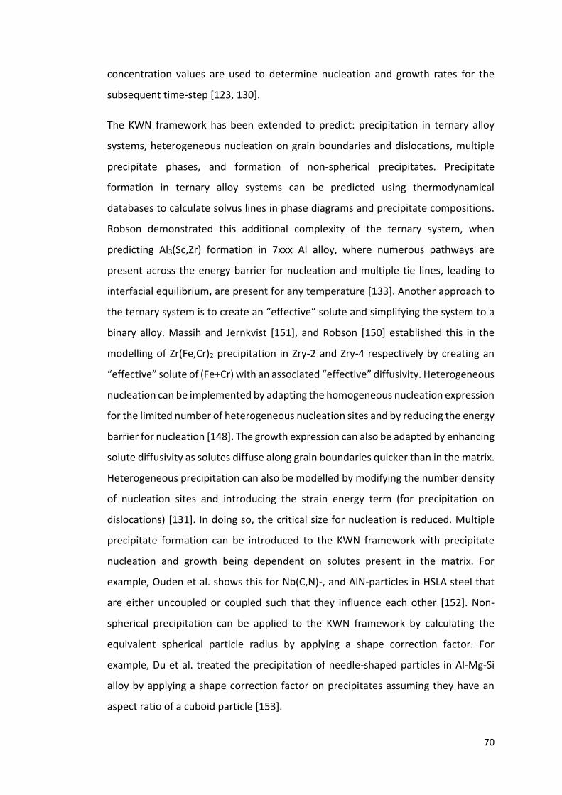
70

concentration values are used to determine nucleation and growth rates for the

subsequent time-step [123, 130].

The KWN framework has been extended to predict: precipitation in ternary alloy

systems, heterogeneous nucleation on grain boundaries and dislocations, multiple

precipitate phases, and formation of non-spherical precipitates. Precipitate

formation in ternary alloy systems can be predicted using thermodynamical

databases to calculate solvus lines in phase diagrams and precipitate compositions.

Robson demonstrated this additional complexity of the ternary system, when

predicting Al3(Sc,Zr) formation in 7xxx Al alloy, where numerous pathways are

present across the energy barrier for nucleation and multiple tie lines, leading to

interfacial equilibrium, are present for any temperature [133]. Another approach to

the ternary system is to create an “effective” solute and simplifying the system to a

binary alloy. Massih and Jernkvist [151], and Robson [150] established this in the

modelling of Zr(Fe,Cr)2 precipitation in Zry-2 and Zry-4 respectively by creating an

“effective” solute of (Fe+Cr) with an associated “effective” diffusivity. Heterogeneous

nucleation can be implemented by adapting the homogeneous nucleation expression

for the limited number of heterogeneous nucleation sites and by reducing the energy

barrier for nucleation [148]. The growth expression can also be adapted by enhancing

solute diffusivity as solutes diffuse along grain boundaries quicker than in the matrix.

Heterogeneous precipitation can also be modelled by modifying the number density

of nucleation sites and introducing the strain energy term (for precipitation on

dislocations) [131]. In doing so, the critical size for nucleation is reduced. Multiple

precipitate formation can be introduced to the KWN framework with precipitate

nucleation and growth being dependent on solutes present in the matrix. For

example, Ouden et al. shows this for Nb(C,N)-, and AlN-particles in HSLA steel that

are either uncoupled or coupled such that they influence each other [152]. Non-

spherical precipitation can be applied to the KWN framework by calculating the

equivalent spherical particle radius by applying a shape correction factor. For

example, Du et al. treated the precipitation of needle-shaped particles in Al-Mg-Si

alloy by applying a shape correction factor on precipitates assuming they have an

aspect ratio of a cuboid particle [153].

71

SPP precipitation kinetics in Zr alloys have been modelled, using a KWN framework,

on Zr-2.5Nb alloy [134] and Zry-4 [150]. Both alloy systems are binary where Zry-4

has an effective solute of (Fe+Cr). Regardless, the KWN models used were altered to

provide simulations of different scenarios. The kinetics model predicting

precipitation in Zr-2.5Nb considers the presence of retained or transformed β-Zr to

β-Nb particles while simulating β-Nb precipitation. This model was calibrated using

experimental data obtained from literature such as [154, 155] (Figure 2-23). In both

circumstances, the predicted measurements agree well with that obtained

experimentally.

Figure 2-23: KWN model developed by Robson [134] used to predict the evolution of SPP

characteristics where: (a) shows the predicted precipitate dimension and spacing when

aged at 500 °C compared against data from [154] and, (b) shows the predicted matrix Nb

evolution against DSC and TEP from [155] and [156]. Adapted from [134].

The simulation predicting precipitation in Zry-4 is a KWN model coupled with model

developed by Motta et al. [157] that predicts the effect that neutron irradiation has

on Zr(Fe,Cr)2 particles. The simulation is not quantitatively accurate hence it did not

need to be calibrated against experimental data. Nevertheless, as with the Zr-2.5Nb

model, this model required input parameters taken from previous research,

72

specifically [107, 151], on modelling the evolution of SPPs. Here, it is assumed that

the particles only dissolve once fully destabilised as a result of the irradiation.

Figure 2-24 illustrates how the Zr(Fe,Cr)2 particles are predicted to evolve with time

with and without exposure to irradiation. It can be seen that for a short period of

time, the simulation results for both non-irradiated and irradiated cases are

matching. Thereafter, the results of the irradiated condition deviate from that

obtained for the non-irradiated condition due to amorphization and dissolution of

SPPs, leading to a reduction in volume fraction and particle number density. It should

be noted that the sharp increase in mean particle radius is due to the fact that the

larger particles take longer to dissolve whilst the particles smaller than the critical

radius dissolve first.

Figure 2-24: Simulated evolution of characteristics of Zr(Fe,Cr)2 particles in Zry-4 at 307 °C

with and without irradiation at a displacement rate of 15 dpa/year where: (a) shows

particle volume fraction and matrix solute level and, (b) shows particle number density

and mean radius. Adapted from [150].

2.8 Summary and the Present Work

Zr alloys can be thermomechanically processed from large Zr sponge through a series

of hot- and cold-work processes, and heat treatments to thin-walled cladding tubes

used in nuclear fuel assemblies. In BWRs, the alloys of interest are Zry-2 and the novel

high Fe alloy, HiFi. Increased Fe content in HiFi is the only difference between the

two alloys.

73

Two SPP types form: hexagonal Zr(Fe,Cr)2 and tetragonal Zr2(Fe,Ni). This is well-

recognized for Zry-2 while not so for HiFi. At times, clusters of SPPs form in Zry-2

where one Zr2(Fe,Ni) in contact with one or multiple Zr(Fe,Cr)2 particles. Further, SPP

morphology and distribution changes throughout processing where they are more

irregularly shaped and heterogeneously distributed in early processing stages while

more spherical and homogeneously distributed SPPs are observed in later stages or

after higher and/or longer anneals.

SPPs have characteristics such as mean size, volume fraction, mean solute

concentration, SPP type, and chemistry. SPP characterization is performed using a

number of experimental techniques. SEM and (S)TEM can thus far directly image

SPPs (without reliably distinguishing SPP types), leading to determination of SPP

mean size, and volume fraction though SPP type and accurate chemical analysis can

only be determined by diffraction in TEM thus far. APT can also directly determine a

number of SPP characteristics though the limited sample geometry leads to reduced

SPP counts. TEP, DSC, XRD and SAXS are indirect methods of examining

characteristics such as mean matrix chemistry, SPP volume fraction, and SPP type

with varying sample volumes. These methods can complement electron microscopy

analysis on SPPs though the required time for sample preparation and analysis varies.

Different thermomechanical processing stages affect SPP characteristics. Water

quenching from temperatures at the β-Zr phase leads to lath structures and small

SPP formation on grain boundaries. Subsequent hot extrusion can affect SPP size and

distribution, and lead to distorted microstructures depending on the temperature

and reduction of the process. The degree of reduction in cold pilgering affects the

linearity or distribution of SPPs though it is questioned whether SPP sizes are affected

by the degree of cold work. Application of heat treatments tend to increase the mean

size of SPPs, and SPP volume fraction also increases up to a point when it stays

constant – the onset of SPP coarsening. The effect of subsequent heat treatments on

SPP size is captured using 𝛸CAP though scatter is observed on mean SPP sizes for the

same 𝛸CAP value. This leads to the introduction of 𝛸SOCAP, a supposedly more

accurate representation of how heat treatments affect SPP size. The resulting SPP

distributions that are skewed small sizes (< 100 nm) lead to improved nodular

74

corrosion resistance while that skewed to large sizes (> 100 nm) lead to improved

uniform corrosion resistance. Irradiation leads to SPP amorphization. Re-distribution

of solutes is possible with re-precipitation of SPPs, leading to PSDs skewed to small

sizes and thus improved corrosion performance.

Numerous kinetics models have been developed to predict SPP kinetics. The JMAK

model is a simple analytical approach that describes SPP kinetics in the form of single

transformation parameter between 0 (untransformed) and 1 (fully transformed)

though only average values of characteristics such as SPP size are expressed. The LSW

theory predicts the SPP PSD after an infinite quantity of time though the onset of this

has been shown to take place well after the onset of particle coarsening. Kahlweit’s

theory is thought to provide a better fit to SPP behaviour. Finally, the KWN

framework is versatile and allows for further modifications such as the inclusion of

heterogeneous nucleation sites, and multiple SPP types. However, precipitation

kinetics of SPPs in Zry-2 have not been modelled extensively where the SPP types are

dependent on each other due to the presence of Fe.

The aim of the present work is to utilise the technological advances in electron

microscopy and differentiate the different SPP type in Zry-2 and HiFi. This can be

complimented with easy, reproducible techniques such as TEP and DSC, both of

which have not extensively been used to determine SPP characteristics in Zry-2 and

HiFi. More detailed information of SPP characteristics can therefore be produced at

all stages of thermomechanical processing from the β-quenched condition to the

final cladding tube. Such data can be used to calibrate a unique precipitation kinetics

model that has been developed to predict the SPP kinetics in both Zry-2 and HiFi,

allowing for an enhanced understanding of the correlation between heat treatments

and SPP size.

75

3 Experimental Methods

3.1 Material

In this present work, Zry-2 and HiFi were analysed in the condition as supplied by

Sandvik AB. Table 3-1 displays the composition of the aforementioned Zr alloys. As

mentioned in Section 2.3, oxygen is added to the alloy in order to improve material

strength via solution strengthening [27]. It should be noted that the main impurities

in both alloys are: silicon (100 wppm), and carbon (100 wppm). Hydrogen

concentration in the alloys was not measured at any processing stage though it is

thought that this is less than that stated in the ASTM specification limits

(< 25 wppm) [158].

Table 3-1: Composition of Zry-2 and HiFi (wt%).

Sn Fe Cr O Ni Zr

Zry-2 1.3 0.18 0.12 0.12 0.055 Balance

HiFi 1.3 0.40 0.12 0.12 0.055 Balance

3.2 Sample Preparation

3.2.1 Mechanical Polishing for Scanning Electron Microscopy

Mechanical polishing was performed to generate a mirror-like finish on the sample

surface for high resolution scanning electron microscopy. It should be noted that

electropolishing of SEM samples was not performed since SPPs have the tendency to

pull out from the matrix. This would lead to a reduction in SPPs counts and inaccurate

PSDs. SEM imaging at low accelerating voltages on mechanically polished samples

can lead to the formation hydrocarbon deposition (Figure 3-1). If this is thick enough,

SEM imaging would be adversely affected [159]. Therefore, certain steps were

performed in mechanical polishing to minimise this.

76

Figure 3-1: Hydrocarbon contamination and presence of colloidal silica particles in SEM

image.

Firstly, the sample was mounted in a thermoplastic resin composed of poly(methyl

methacrylate). Using P800 silicon carbon (SiC) abrasive paper, the sample was ground

flat until parallel, unidirectional scratches are visible. The sample was polished with

6 µm monocrystalline oil-based diamond suspension until all P800 scratches were

removed from the sample surface. Thereafter, polishing was conducted using 3 µm

monocrystalline oil-based diamond suspension until the majority of 6 μm scratches

were removed. 1 µm monocrystalline oil-based diamond suspension polishing just

before initial pit formation was the next step. Afterward, 0.25 µm monocrystalline

oil-based diamond suspension polishing was performed to remove the majority of

1 μm scratches. The sample was then etched in a solution of diluted Kroll’s reagent

(2 ml HF, 4 ml HNO3, and 188 ml H2O) for a fraction of a second. The final polishing

step was in water-based alkaline colloidal silica (pH 9-11) with particles of 60 nm,

resulting in a scratch-free sample surface with minimal mechanical damage.

Thereafter, the sample was cleaned thoroughly to remove any residual colloidal silica

particles present on the sample surface (Figure 3-1). This is conducted by cleaning

the sample in water and soap for at least 10 minutes. The sample is removed from

the thermoplastic resin using a hot plate at a temperature above the glass transition

temperature (> 105 °C). If the sample is left in the resin, hydrocarbons are formed

when the electron beam interacts with the resin and thus contrast is minimised in

the electron images. To ensure that the samples are clean, they are then placed in a

beaker of isopropanol and left in an ultrasonic bath prior to adhering on an

77

aluminium SEM stub with silver paint. Finally, the samples are stored in a vacuum

desiccator after sample preparation to minimise contact with air and dirt. The final

cleaning step is performed in the SEM where a plasma cleaner is operated to prevent

hydrocarbon formation.

3.2.2 Electropolishing STEM Samples

STEM foils were prepared by grinding the material of interest to a thickness of

approximately 100 μm using P800 SiC abrasive paper. 3 mm discs were then

mechanically punched from the material. These samples were subsequently

electropolished using the twin-jet Tenupol-5 electropolisher in a solution of 10 %

perchloric acid, 20 % 2-butoxyethanol in ethanol at -5 °C [160]. Electropolishing is

complete when the discs have perforated and electron transparent regions have

formed.

As with SEM samples, STEM foils are susceptible to contamination in the microscope.

This is minimised by storing the foils in a vacuum desiccator after electropolishing

and plasma cleaning the foils prior to use in the STEM. It should be noted that plasma

cleaning should not be performed for too long since this could remove any electron

transparent regions formed after electropolishing.

3.2.3 DSC Samples

DSC samples are limited to a maximum diameter of 5 mm. β-quenched Zry-2 and HiFi

supplied by Sandvik AB were cut into small pieces. Thereafter, P800 SiC abrasive

paper was used to carefully grind the small pieces to dimensions of

4 mm x 4 mm x 1 mm.

3.2.4 TEP Samples

TEP measurements were performed on β-quenched material. The TEP specimens

were EDM cut from a block β-quenched material supplied by Sandvik AB (initial

dimensions of 85 mm x 30 mm x 10 mm) to 85 mm x 5mm x 2mm matchsticks, with

the resulting surface damage being carefully removed using P800 SiC abrasive paper.

Since the cooling rate between the outer surface and the centre of the β-quenched

78

block is different, an additional β-quench was performed on the matchsticks. The

heat treatment was performed using a horizontal Carbolite tube furnace in an argon

atmosphere from room temperature to 1150 °C. This temperature was chosen since

this replicates the β-heat treatment used in industry, provides a good margin from

the α-Zr to β-Zr phase transformation, and allows the dissolution of all precipitates

and impurities present in the alloys [38]. A rapid water quench is performed once the

maximum temperature is reached by dragging the samples from the furnace to a

bucket of cold water. This minimises the formation of SPPs. SPP formation is not

thought to be fully suppressed since the cooling rate is not larger than 2000 °C/s [37].

The quenching rate of the β-quenching procedure was established by measuring the

temperature profile of the sample. Figure 3-2 illustrates this. The cooling rate could

not be established therefore it is thought to be approximately 1500 °C/s [37]. It

should be noted that the matchsticks are left in the argon atmosphere for at least

30 minutes prior to the heat treatment to minimise contamination with oxygen and

minimise oxide growth.

Figure 3-2: β-heat treatment and quench temperature profile used for TEP samples.

Following the β-heat treatment, the matchstick thickness was reduced to

approximately 1 mm using SiC paper ranging from P120 to P800 grit. Thereafter,

different heat treatments were performed on different matchsticks, using the

Carbolite tube furnace in an argon atmosphere, to promote SPP formation. Finally,

the matchsticks were reduced to a thickness of 0.5 ± 0.05 mm with P800 SiC paper.

79

Prior to TEP measurements, the matchsticks were lightly ground with P1200 SiC

abrasive paper, to remove surface oxides, and finally cleaned in ethanol.

3.3 Scanning Electron Microscopy

Optical microscopy has the advantages of identifying features at a very low

magnification such as scratches and pitting. However, optical microscopy has

limitations with regards to imaging SPPs in Zr alloys. SPPs are in the order of 100 nm

and thus a much higher magnification is required. This higher magnification is

attained by using an electron probe where the electrons are emitted from either a

tungsten filament or a field emission gun.

Here, the Zeiss Merlin SEM, with a field emission gun (FEG), was utilised to image and

identify the SPPs. This microscope is capable of accelerating electrons to voltages

within the range of 0.02-30 keV. The Zeiss Merlin SEM utilises a Gemini 2 column

which consists of a double condenser lens system (as opposed to the single

condenser lens used in the majority of SEM columns). Significantly higher probe

currents (3 pA – 40 nA) can therefore be used. In addition, a much smaller probe size

can be formed since there is an additional electron crossover point in the

column [161, 162]. The objective lens system, below the condenser lens system,

produces the final spot size on the sample of interest. This system consists of a double

deflection coil (allows the beam to be rastered in the x- and y-axes), a stigmator

(produces symmetrical magnetic field), and an aperture (controls electron beam

current). Figure 3-3 illustrates a schematic of the SEM configuration.

80

Figure 3-3: SEM configuration where: a) illustrates the schematic of the whole SEM column,

and b) illustrates the schematic of the objective lens system, adapted from [163].

Images are generated when specific signals, produced from the interaction between

electrons in the beam and the sample, are collected by detectors either located in

the SEM chamber or SEM gun column. As displayed in Figure 3-4, secondary electrons

(SEs), backscatter electrons (BSEs) and characteristic x-rays are the signals of interest.

SEs are produced due to inelastic interactions between the electrons in the beam and

the sample surface and therefore have energies less than 50 eV. This type of signal

provides sample topographical information. BSEs are produced by elastic scattering

events and have a much higher energy than SEs, providing compositional contrast,

while the generated x-rays provide elemental information [163]. In this project, both

Zry-2 and HiFi consist of SPPs with different compositions. Therefore, the signals of

interest are BSEs and characteristic x-rays.

81

Figure 3-4: Signals produced in interaction volume generated in sample.

Since SPPs in Zr alloys are generally less than 1 µm in size, a low accelerating voltage

is required. This leads to a smaller interaction volume, as illustrated in Figure 3-5.

Here, Monte Carlo simulations in the CASINO software package [164] was used to

simulate the theoretical interaction volume size in Zr alloys at 3 keV and 20 keV. With

a SPP with a thickness of, for example, 50 nm from the surface, more information is

obtained from using a 3 keV accelerating voltage. The whole interaction volume

would be encompassed within the SPP. Thus detection of signals from the matrix

below the SPP is limited. On the other hand, the interaction volume generated from

the 20 keV beam provides more matrix information beneath the SPP.

82

Figure 3-5: Sample interaction volume size with an accelerating voltage of: a) 3 keV, and b)

20 keV.

3.3.1 Energy and Angle Selective Backscatter Detector

The energy and angle selective backscatter (ESB) detector, located in the SEM gun

column (Figure 3-6), is located above the In-lens detector, a SE detector that collects

the low energy secondary electrons. The ESB detector is capable of obtaining surface-

sensitive compositional information.

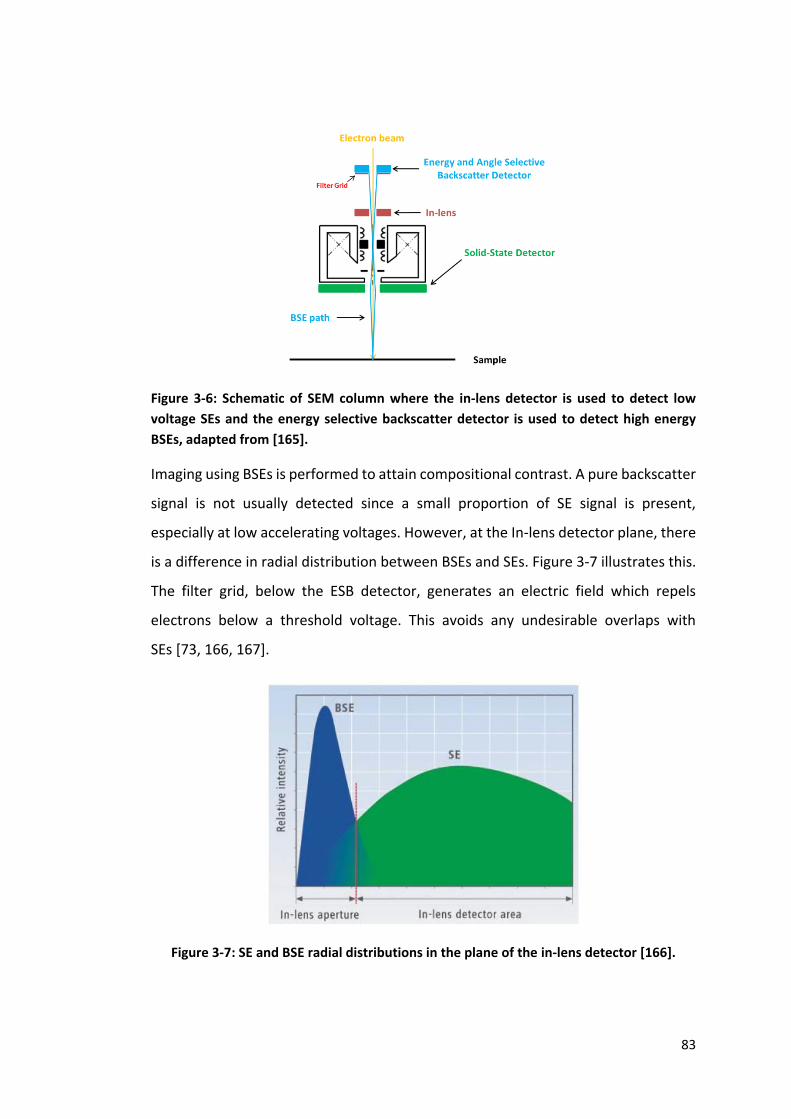
83

Figure 3-6: Schematic of SEM column where the in-lens detector is used to detect low

voltage SEs and the energy selective backscatter detector is used to detect high energy

BSEs, adapted from [165].

Imaging using BSEs is performed to attain compositional contrast. A pure backscatter

signal is not usually detected since a small proportion of SE signal is present,

especially at low accelerating voltages. However, at the In-lens detector plane, there

is a difference in radial distribution between BSEs and SEs. Figure 3-7 illustrates this.

The filter grid, below the ESB detector, generates an electric field which repels

electrons below a threshold voltage. This avoids any undesirable overlaps with

SEs [73, 166, 167].

Figure 3-7: SE and BSE radial distributions in the plane of the in-lens detector [166].

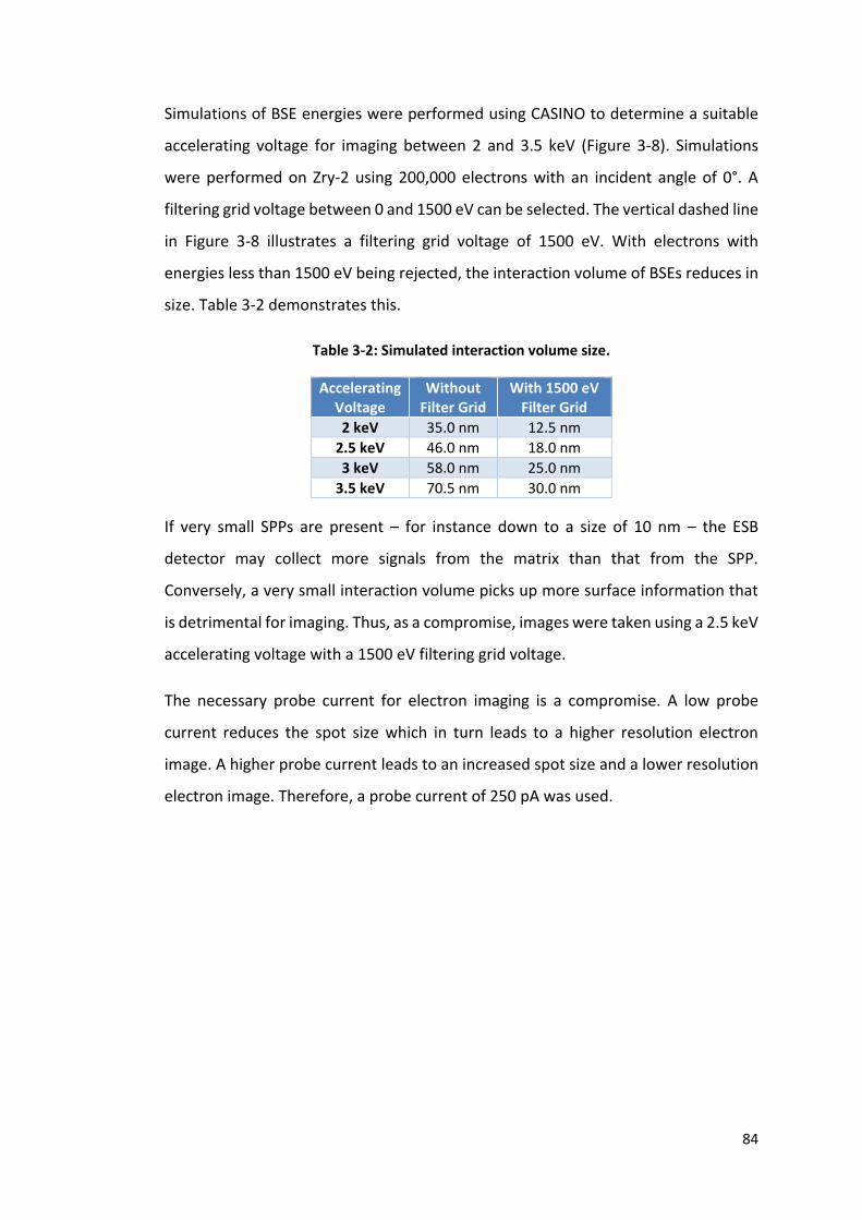
84

Simulations of BSE energies were performed using CASINO to determine a suitable

accelerating voltage for imaging between 2 and 3.5 keV (Figure 3-8). Simulations

were performed on Zry-2 using 200,000 electrons with an incident angle of 0°. A

filtering grid voltage between 0 and 1500 eV can be selected. The vertical dashed line

in Figure 3-8 illustrates a filtering grid voltage of 1500 eV. With electrons with

energies less than 1500 eV being rejected, the interaction volume of BSEs reduces in

size. Table 3-2 demonstrates this.

Table 3-2: Simulated interaction volume size.

Accelerating Voltage

Without Filter Grid

With 1500 eV Filter Grid

2 keV 35.0 nm 12.5 nm

2.5 keV 46.0 nm 18.0 nm

3 keV 58.0 nm 25.0 nm

3.5 keV 70.5 nm 30.0 nm

If very small SPPs are present – for instance down to a size of 10 nm – the ESB

detector may collect more signals from the matrix than that from the SPP.

Conversely, a very small interaction volume picks up more surface information that

is detrimental for imaging. Thus, as a compromise, images were taken using a 2.5 keV

accelerating voltage with a 1500 eV filtering grid voltage.

The necessary probe current for electron imaging is a compromise. A low probe

current reduces the spot size which in turn leads to a higher resolution electron

image. A higher probe current leads to an increased spot size and a lower resolution

electron image. Therefore, a probe current of 250 pA was used.

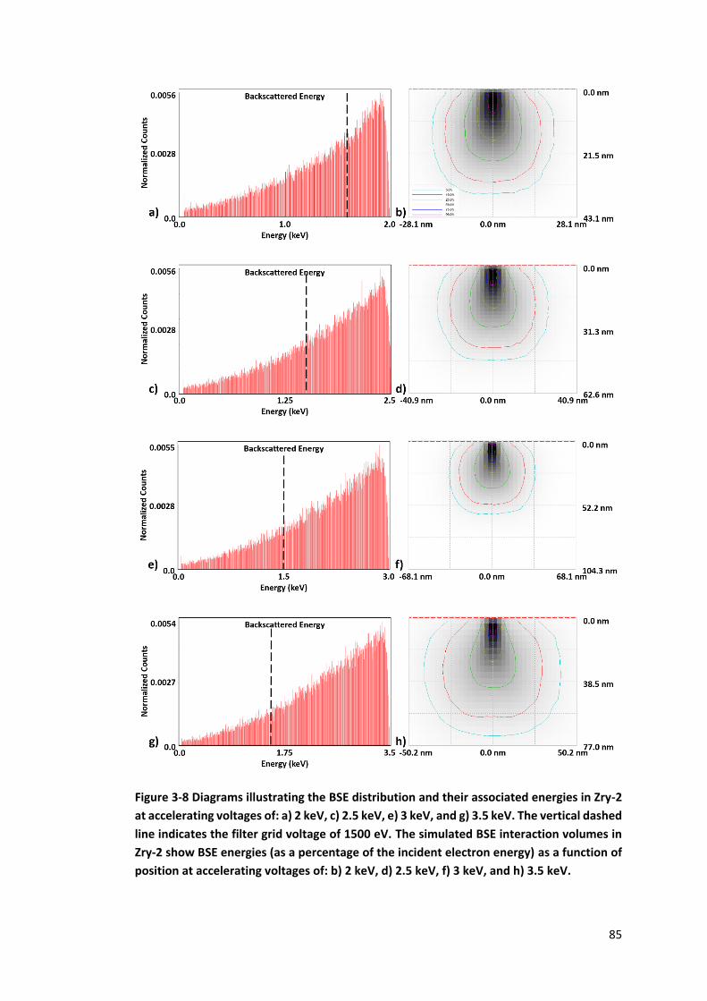
85

Figure 3-8 Diagrams illustrating the BSE distribution and their associated energies in Zry-2

at accelerating voltages of: a) 2 keV, c) 2.5 keV, e) 3 keV, and g) 3.5 keV. The vertical dashed

line indicates the filter grid voltage of 1500 eV. The simulated BSE interaction volumes in

Zry-2 show BSE energies (as a percentage of the incident electron energy) as a function of

position at accelerating voltages of: b) 2 keV, d) 2.5 keV, f) 3 keV, and h) 3.5 keV.

86

3.3.2 Electron Backscatter Diffraction

Electron backscatter diffraction (EBSD) was used to identify the crystallography of

the SPPs in HiFi. It should be noted that this was not performed on Zry-2 since the

SPPs in this alloy have been identified previously using TEM or x-ray synchrotron

studies [22, 61–63, 65, 66]. Inelastically scattered BSEs that diffract according to

Bragg’s law, for specific crystallographic planes, lead to the formation of Kikuchi

diffraction patterns with specific interplanar angles. Tilting the sample by 70° allows

the inelastic BSEs to escape from the sample surface, reduce electron absorption and

maximise Kikuchi pattern indexing. The experimentally formed Kikuchi patterns are

then compared to interplanar angles of theoretical Kikuchi patterns that are based

on pre-determined crystal structures.

Given that the SPPs are smaller than 1 μm in size, an accelerating voltage smaller

than that used for grain orientation analysis [39, 117, 168–170] was used to improve

resolution. In this study, EBSD was performed using a 10 keV accelerating voltage, at

a current of 4 nA, and working distance of 15 mm. A step size of 20 nm was selected,

generating 3-4 points per SPP. EBSD patterns were obtained using the Oxford

Instruments Nordlys S detector.

3.3.3 Energy Dispersive X-Ray Spectroscopy

Energy dispersive x-ray spectroscopy (EDX) is utilised to perform elemental analysis

on features in samples. When a primary electron from the electron beam interacts

with atoms, an electron from the inner shell is ejected and the atom is energised. To

return it to its ground state, the vacancy in the inner shell is filled by an outer shell

electron and the associated characteristic X-ray is released, as shown in Figure 3-9(a).

Characteristic x-rays are classified depending on the electron jump from outer shell

to inner shell. Figure 3-9(b) illustrates this where an electron jumping to the adjacent

inner shell is termed α x-rays, and an electron jumping two or three inner shells are

termed β- and γ- x-rays respectively.

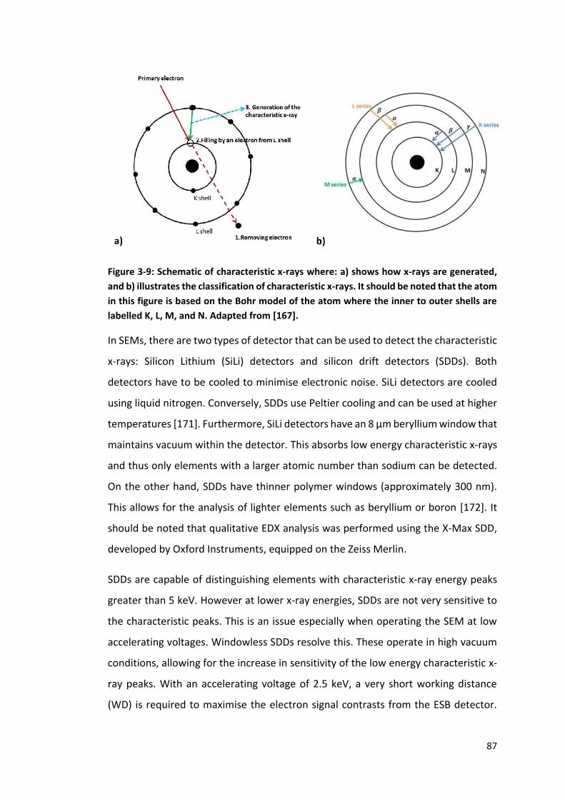
87

Figure 3-9: Schematic of characteristic x-rays where: a) shows how x-rays are generated,

and b) illustrates the classification of characteristic x-rays. It should be noted that the atom

in this figure is based on the Bohr model of the atom where the inner to outer shells are

labelled K, L, M, and N. Adapted from [167].

In SEMs, there are two types of detector that can be used to detect the characteristic

x-rays: Silicon Lithium (SiLi) detectors and silicon drift detectors (SDDs). Both

detectors have to be cooled to minimise electronic noise. SiLi detectors are cooled

using liquid nitrogen. Conversely, SDDs use Peltier cooling and can be used at higher

temperatures [171]. Furthermore, SiLi detectors have an 8 µm beryllium window that

maintains vacuum within the detector. This absorbs low energy characteristic x-rays

and thus only elements with a larger atomic number than sodium can be detected.

On the other hand, SDDs have thinner polymer windows (approximately 300 nm).

This allows for the analysis of lighter elements such as beryllium or boron [172]. It

should be noted that qualitative EDX analysis was performed using the X-Max SDD,

developed by Oxford Instruments, equipped on the Zeiss Merlin.

SDDs are capable of distinguishing elements with characteristic x-ray energy peaks

greater than 5 keV. However at lower x-ray energies, SDDs are not very sensitive to

the characteristic peaks. This is an issue especially when operating the SEM at low

accelerating voltages. Windowless SDDs resolve this. These operate in high vacuum

conditions, allowing for the increase in sensitivity of the low energy characteristic x-

ray peaks. With an accelerating voltage of 2.5 keV, a very short working distance

(WD) is required to maximise the electron signal contrasts from the ESB detector.

88

Therefore, the SDD is required to operate and collect x-rays from a short WD. The X-

Max Extreme detector, also developed by Oxford Instruments, allows for such data

acquisition [173]. Both the X-Max SDDs and an X-Max Extreme detector are equipped

on the Zeiss Merlin though only the X-Max Extreme detector is used in this study.

Here, a probe current between 200 pA and 800 pA is used. This improves the

acquisition rate compared to the probe current used for electron imaging. The

sample WD is at 4.5 mm for the X-Max Extreme detector. This was kept at the same

value for all SEM imaging.

The elements of interest in Zry-2 and HiFi are Zr, Fe, Cr and Ni. The characteristic x-

ray energy lines produced for these elements are displayed in Table 3-3. The

characteristic x-rays of interest at a 2.5 keV accelerating voltage are the L series x-

rays.

Table 3-3: Characteristic x-ray energy lines (keV) [174].

Kα Kβ Lα Lβ Mα

Zr 15.775 17.667 2.042 2.124 -

Fe 6.403 7.057 0.705 0.719 -

Cr 5.415 5.947 0.573 0.583 -

Ni 7.478 8.265 0.852 0.869 -

3.4 Scanning Transmission Electron Microscopy

The observed features in SEMs are reflected from the sample surface. In TEMs, such

features are seen through the thickness of electron transparent foils. The regions of

interest in the foils are approximately 100 nm thick. Here, the accelerating voltage is

much greater than that in the SEM and thus the electron wavelength is smaller.

Table 3-4 depicts this where Equation 3-1 calculates the electron wavelength [76].

𝜆 = ℎ

√2𝑚𝑒𝑉≈ √

(1.5 nm2V−1)

𝑉 (3-1)

Table 3-4: Electron wavelength as a function of accelerating voltage.

Voltage (keV) Electron Wavelength (nm)

5 0.0173

10 0.0122

20 0.0086

200 0.0027

89

where ℎ is Planck’s constant, 𝑚 is the mass of an electron, 𝑒 is the electronic charge,

and 𝑉 is the accelerating voltage. The reduction in wavelength in turn reduces the

spot size of the beam and enhances resolution. The resulting image is produced from

the transmitted electrons (both elastically and in-elastically scattered) below the

sample.

SPP imaging was performed using the FEI Talos F200X G2 in STEM mode. As with the

SEM, the electron beam is generated from the FEG though the beam is at an

accelerating voltage of 200 keV. The beam passes through the condenser lens

system, keeping it parallel. Thereafter, the beam passes through the mini condenser

lens – producing a convergent or parallel beam – and the objective lens system which

forms a diffraction pattern of the specimen in the back focal plane. This diffraction

pattern is then converted into an image and magnified by the intermediate and

projector lenses. In STEM, like in a SEM, the condenser and objective lens systems

are used to create a fine convergent beam which rasters over the specimen by

scanning coils.

3.4.1 STEM Imaging

The bright field (BF) detector is mainly used in this study. It is aligned with the

microscope’s optic axis, below the projector lens. The BF detector collects

transmitted electrons that have not diffracted. Electrons diffracted from the optic

axis are collected using an annular dark-field (ADF) detector. Electron detection using

ADF detectors is defined by the detector collection angle and the inner radius of the

detector. Electrons diffracted at large angles are collected using the high angle ADF

(HAADF) detector. This provides mass-thickness contrast due to the Rutherford

scattering – or incoherent elastic scattering – of electrons [76]. In turn, the HAADF

detector provides atomic number (Z) contrast.

3.4.2 STEM-EDX

In this study, STEM-EDX was performed using the Super-X EDX detector system

equipped on the FEI Talos F200X G2. This system consists of four windowless SDDs in

the vicinity of the specimen. This provides a collection angle of approximately

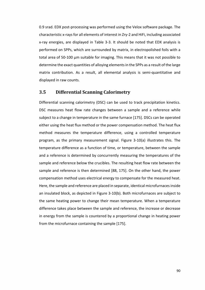
90

0.9 srad. EDX post-processing was performed using the Velox software package. The

characteristic x-rays for all elements of interest in Zry-2 and HiFi, including associated

x-ray energies, are displayed in Table 3-3. It should be noted that EDX analysis is

performed on SPPs, which are surrounded by matrix, in electropolished foils with a

total area of 50-100 μm suitable for imaging. This means that it was not possible to

determine the exact quantities of alloying elements in the SPPs as a result of the large

matrix contribution. As a result, all elemental analysis is semi-quantitative and

displayed in raw counts.

3.5 Differential Scanning Calorimetry

Differential scanning calorimetry (DSC) can be used to track precipitation kinetics.

DSC measures heat flow rate changes between a sample and a reference while

subject to a change in temperature in the same furnace [175]. DSCs can be operated

either using the heat flux method or the power compensation method. The heat flux

method measures the temperature difference, using a controlled temperature

program, as the primary measurement signal. Figure 3-10(a) illustrates this. The

temperature difference as a function of time, or temperature, between the sample

and a reference is determined by concurrently measuring the temperatures of the

sample and reference below the crucibles. The resulting heat flow rate between the

sample and reference is then determined [88, 175]. On the other hand, the power

compensation method uses electrical energy to compensate for the measured heat.

Here, the sample and reference are placed in separate, identical microfurnaces inside

an insulated block, as depicted in Figure 3-10(b). Both microfurnaces are subject to

the same heating power to change their mean temperature. When a temperature

difference takes place between the sample and reference, the increase or decrease

in energy from the sample is countered by a proportional change in heating power

from the microfurnace containing the sample [175].

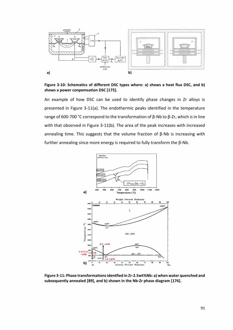
91

Figure 3-10: Schematics of different DSC types where: a) shows a heat flux DSC, and b) shows a power conpemsation DSC [175].

An example of how DSC can be used to identify phase changes in Zr alloys is

presented in Figure 3-11(a). The endothermic peaks identified in the temperature

range of 600-700 °C correspond to the transformation of β-Nb to β-Zr, which is in line

with that observed in Figure 3-11(b). The area of the peak increases with increased

annealing time. This suggests that the volume fraction of β-Nb is increasing with

further annealing since more energy is required to fully transform the β-Nb.

Figure 3-11: Phase transformations identfied in Zr-2.5wt%Nb: a) when water quenched and subsequently annealed [89], and b) shown in the Nb-Zr phase diagram [176].

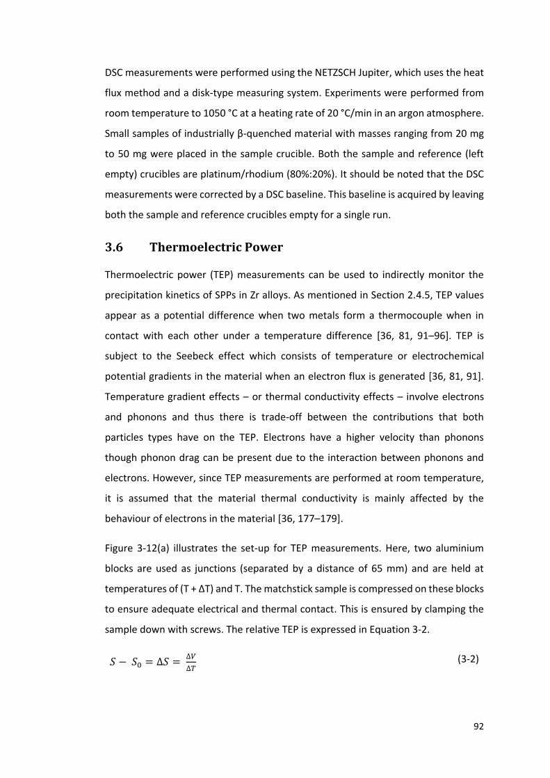
92

DSC measurements were performed using the NETZSCH Jupiter, which uses the heat

flux method and a disk-type measuring system. Experiments were performed from

room temperature to 1050 °C at a heating rate of 20 °C/min in an argon atmosphere.

Small samples of industrially β-quenched material with masses ranging from 20 mg

to 50 mg were placed in the sample crucible. Both the sample and reference (left

empty) crucibles are platinum/rhodium (80%:20%). It should be noted that the DSC

measurements were corrected by a DSC baseline. This baseline is acquired by leaving

both the sample and reference crucibles empty for a single run.

3.6 Thermoelectric Power

Thermoelectric power (TEP) measurements can be used to indirectly monitor the

precipitation kinetics of SPPs in Zr alloys. As mentioned in Section 2.4.5, TEP values

appear as a potential difference when two metals form a thermocouple when in

contact with each other under a temperature difference [36, 81, 91–96]. TEP is

subject to the Seebeck effect which consists of temperature or electrochemical

potential gradients in the material when an electron flux is generated [36, 81, 91].

Temperature gradient effects – or thermal conductivity effects – involve electrons

and phonons and thus there is trade-off between the contributions that both

particles types have on the TEP. Electrons have a higher velocity than phonons

though phonon drag can be present due to the interaction between phonons and

electrons. However, since TEP measurements are performed at room temperature,

it is assumed that the material thermal conductivity is mainly affected by the

behaviour of electrons in the material [36, 177–179].

Figure 3-12(a) illustrates the set-up for TEP measurements. Here, two aluminium

blocks are used as junctions (separated by a distance of 65 mm) and are held at

temperatures of (T + ΔT) and T. The matchstick sample is compressed on these blocks

to ensure adequate electrical and thermal contact. This is ensured by clamping the

sample down with screws. The relative TEP is expressed in Equation 3-2.

𝑆 − 𝑆0 = ∆𝑆 = ∆𝑉

∆𝑇 (3-2)

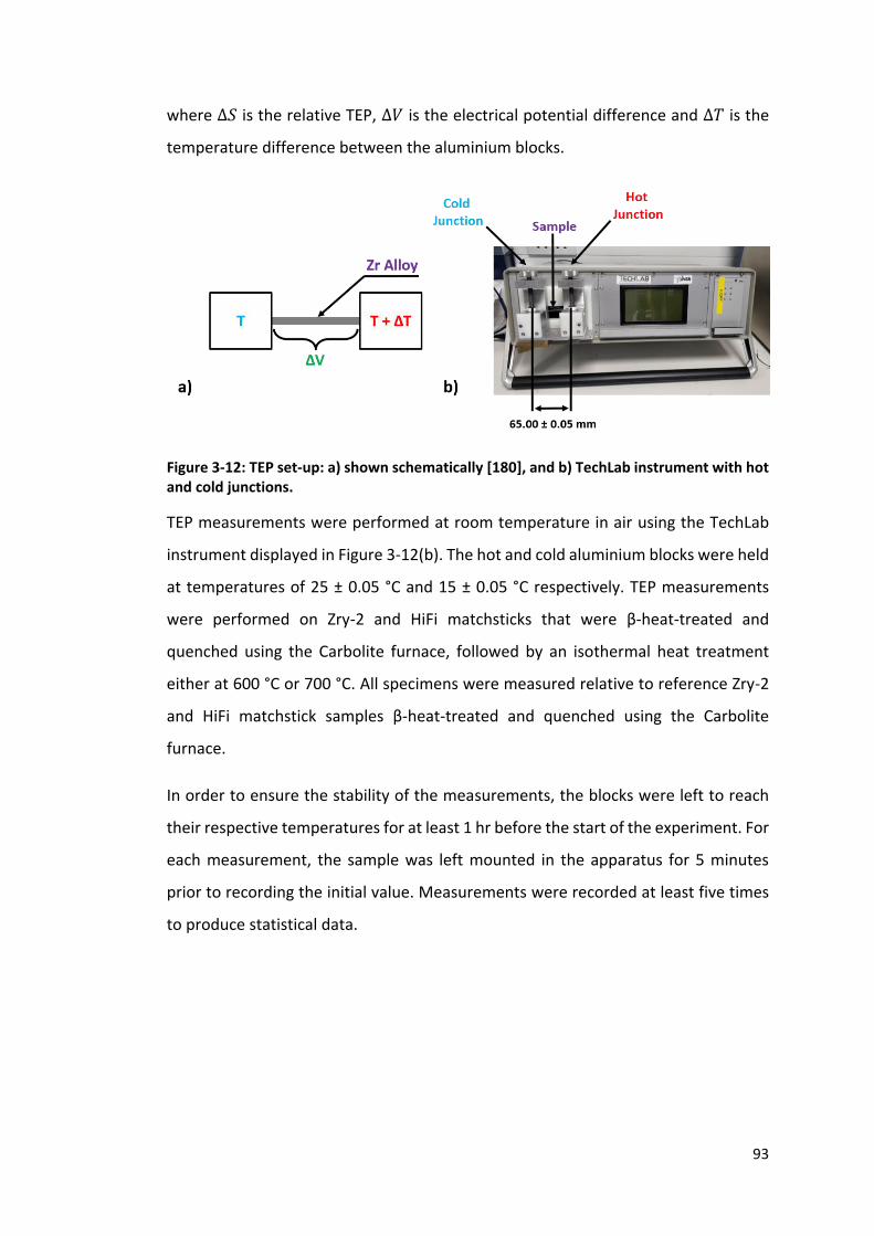
93

where ∆𝑆 is the relative TEP, ∆𝑉 is the electrical potential difference and ∆𝑇 is the

temperature difference between the aluminium blocks.

Figure 3-12: TEP set-up: a) shown schematically [180], and b) TechLab instrument with hot and cold junctions.

TEP measurements were performed at room temperature in air using the TechLab

instrument displayed in Figure 3-12(b). The hot and cold aluminium blocks were held

at temperatures of 25 ± 0.05 °C and 15 ± 0.05 °C respectively. TEP measurements

were performed on Zry-2 and HiFi matchsticks that were β-heat-treated and

quenched using the Carbolite furnace, followed by an isothermal heat treatment

either at 600 °C or 700 °C. All specimens were measured relative to reference Zry-2

and HiFi matchstick samples β-heat-treated and quenched using the Carbolite

furnace.

In order to ensure the stability of the measurements, the blocks were left to reach

their respective temperatures for at least 1 hr before the start of the experiment. For

each measurement, the sample was left mounted in the apparatus for 5 minutes

prior to recording the initial value. Measurements were recorded at least five times

to produce statistical data.

94

4 Experimental Characterization of Second Phase

Particles

This section presents the results obtained from the experimental procedures

outlined in Section 3. Here, the different experimental techniques are reviewed and

compared with regards to their suitability to the characterization of SPPs in Zry-2 and

HiFi.

4.1 Electron Microscopy

4.1.1 SEM

4.1.1.1 HiFi

Figure 4-1 shows SPPs in HiFi imaged using the ESB detector equipped on the Zeiss

Merlin. The highlighted SPPs observed in this electron image are displayed as two

separate grayscale values against the matrix The darker particle is shown to be rich

in Fe and Cr, while the brighter particle is rich in Fe and Ni. Both SPPs types are

deficient in Zr. It should be noted that the Extreme detector has not been calibrated

for quantitative analysis. Therefore, this EDX mapping analysis is qualitative and the

EDX maps do not show the quantity of elements present in the SPPs. EBSD mapping

of the darker SPP shows that it has a hexagonal crystallographic structure with the

following lattice parameters: a = 0.50 nm, and c = 0.82 nm. EBSD mapping of the

brighter SPP shows that it has a body-centred tetragonal crystallographic structure

with lattice parameters: a = 0.648 nm, and c = 0.526 nm. This is equivalent to the

Zr(Fe,Cr)2 and Zr2(Fe,Ni) particles identified by Motta et al. when using synchrotron

radiation to study SPPs in Zr alloys [49]. It should be noted that the unindexed regions

in the EBSD maps (black pixels) result either from overlapping Kikuchi patterns from

the SPP and matrix, or insufficient indexing.

95

Figure 4-1: BSE image of SPPs in HiFi with associated EDX and EBSD of the different SPP

types.

The difference in grayscale between the SPP types result from differences in the

electron backscattering coefficient. This is defined as the proportion of primary

electrons (energies > 50 eV) that interact with atoms in the sample, both elastically

and inelastically, and reflect back through the sample surface. At accelerating

voltages above 5 keV, the backscattering coefficient increases with increasing atomic

number (𝑍) meaning that higher 𝑍 phases appear brighter in BSE images, as shown

in Figure 4-2(a). Figure 4-2(b) shows that at accelerating voltages less than 2 keV, the

backscattering coefficient behaviour changes where higher 𝑍 materials have smaller

interaction volume sizes than lower 𝑍 materials at the same accelerating voltage due

to a higher number of elastic scattering events. Though, given that BSE imaging in

this study was performed at 2.5 keV, the backscattering coefficient of each material

in Figure 4-2(b) can be extended slightly. This shows that the behaviour of the back

scattering coefficient is similar to that observed in Figure 4-2(a) where this value

increases with increasing 𝑍 [73]. Since the average atomic number for both Zr(Fe,Cr)2

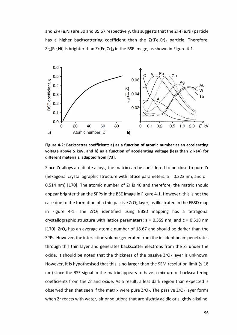
96

and Zr2(Fe,Ni) are 30 and 35.67 respectively, this suggests that the Zr2(Fe,Ni) particle

has a higher backscattering coefficient than the Zr(Fe,Cr)2 particle. Therefore,

Zr2(Fe,Ni) is brighter than Zr(Fe,Cr)2 in the BSE image, as shown in Figure 4-1.

Figure 4-2: Backscatter coefficient: a) as a function of atomic number at an accelerating

voltage above 5 keV, and b) as a function of accelerating voltage (less than 2 keV) for

different materials, adapted from [73].

Since Zr alloys are dilute alloys, the matrix can be considered to be close to pure Zr

(hexagonal crystallographic structure with lattice parameters: a = 0.323 nm, and c =

0.514 nm) [170]. The atomic number of Zr is 40 and therefore, the matrix should

appear brighter than the SPPs in the BSE image in Figure 4-1. However, this is not the

case due to the formation of a thin passive ZrO2 layer, as illustrated in the EBSD map

in Figure 4-1. The ZrO2 identified using EBSD mapping has a tetragonal

crystallographic structure with lattice parameters: a = 0.359 nm, and c = 0.518 nm

[170]. ZrO2 has an average atomic number of 18.67 and should be darker than the

SPPs. However, the interaction volume generated from the incident beam penetrates

through this thin layer and generates backscatter electrons from the Zr under the

oxide. It should be noted that the thickness of the passive ZrO2 layer is unknown.

However, it is hypothesised that this is no larger than the SEM resolution limit (≤ 18

nm) since the BSE signal in the matrix appears to have a mixture of backscattering

coefficients from the Zr and oxide. As a result, a less dark region than expected is

observed than that seen if the matrix were pure ZrO2. The passive ZrO2 layer forms

when Zr reacts with water, air or solutions that are slightly acidic or slightly alkaline.

97

The passive ZrO2 layer most likely formed when the material was mechanically

polished with alkaline colloidal silica solution. To minimise the growth of the oxide,

the colloidal silica polishing step was kept as short as possible.

4.1.1.2 Zircaloy-2

Figure 4-3 shows a BSE image of SPPs in Zry-2. As with that shown in HiFi, the SPPs

observed in this electron image are displayed as two separate grayscale values

against the matrix. As discussed in Section 2.3, Zr(Fe,Cr)2 and Zr2(Fe,Ni) are present

in Zry-2. This is confirmed using EDX analysis where the lighter particles in the BSE

image are shown to be rich in Fe and Ni while the darker particles are rich in Fe and

Cr. The quantity of Zr in both types of particles decreases relative to the matrix. As

with HiFi, the matrix in Figure 4-3 is darker than that expected for Zr due to the

formation of the passive oxide layer.

Figure 4-3: ESB image and associated EDX of SPPs in Zry-2.

4.1.1.3 Particle Size Analysis

From the BSE images, SPPs were counted and their sizes were measured using ImageJ

[181]. Each BSE image had their scale set and then the particle size was determined

by manually drawing around the perimeter of each particle. ImageJ calculated the

area of the particle, the value of which was then converted to an “effective” particle

size (Equation 4-1) assuming that the particle is spherical in nature.

98

𝐷eff = √4 ×𝐴

𝜋 (4-1)

where 𝐷𝑒𝑓𝑓 is the effective particle size, and 𝐴 is the particle area. However, the

effective particle size is not the true particle size since mechanical polishing does not

reveal the real diameter of the sphere. The true particle size can be obtained by

relating the average linear intercept (or the particle size measured in ImageJ) to the

particle’s surface area and volume. This is illustrated in Equation 4-2, as shown by

Tomkeieff [182]:

𝐷eff = 4𝑉SPP

𝑆SPP (4-2)

where 𝑉SPP is the volume of the particle (equal to 4

3𝜋𝑟3 for a spherical particle) and

𝑆SPP is the particle’s surface area (equal to 4𝜋𝑟2 for a spherical particle). This leads

to Equation 4-3:

𝐷eff = 4

3𝑟 (4-3)

The true particle radius, 𝑟, is then converted to true particle diameter (𝐷true) to form

Equation 4-4.

𝐷eff = 2

3𝐷true (4-4)

Or simply:

𝐷true = 3

2𝐷eff (4-5)

Figure 4-4 shows the PSD of the effective and true sizes of both SPP types in the final

cladding material in Zry-2. The error bars on the red histogram bars and cyan

histogram bars show the standard error of the Zr(Fe,Cr)2 number density and

Zr2(Fe,Ni) number density respectively. The error bar on the horizontal red line and

on the horizontal orange line are the standard errors of the mean Zr(Fe,Cr)2 size and

mean Zr2(Fe,Ni) size respectively. The class width, from Gros and Wadier [107], was

determined using Equation 4-6.

𝐷max − 𝐷min

√𝑁 (4-6)

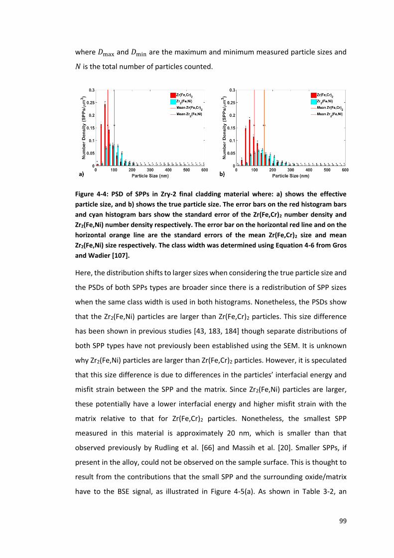
99

where 𝐷max and 𝐷min are the maximum and minimum measured particle sizes and

𝑁 is the total number of particles counted.

Figure 4-4: PSD of SPPs in Zry-2 final cladding material where: a) shows the effective

particle size, and b) shows the true particle size. The error bars on the red histogram bars

and cyan histogram bars show the standard error of the Zr(Fe,Cr)2 number density and

Zr2(Fe,Ni) number density respectively. The error bar on the horizontal red line and on the

horizontal orange line are the standard errors of the mean Zr(Fe,Cr)2 size and mean

Zr2(Fe,Ni) size respectively. The class width was determined using Equation 4-6 from Gros

and Wadier [107].

Here, the distribution shifts to larger sizes when considering the true particle size and

the PSDs of both SPPs types are broader since there is a redistribution of SPP sizes

when the same class width is used in both histograms. Nonetheless, the PSDs show

that the Zr2(Fe,Ni) particles are larger than Zr(Fe,Cr)2 particles. This size difference

has been shown in previous studies [43, 183, 184] though separate distributions of

both SPP types have not previously been established using the SEM. It is unknown

why Zr2(Fe,Ni) particles are larger than Zr(Fe,Cr)2 particles. However, it is speculated

that this size difference is due to differences in the particles’ interfacial energy and

misfit strain between the SPP and the matrix. Since Zr2(Fe,Ni) particles are larger,

these potentially have a lower interfacial energy and higher misfit strain with the

matrix relative to that for Zr(Fe,Cr)2 particles. Nonetheless, the smallest SPP

measured in this material is approximately 20 nm, which is smaller than that

observed previously by Rudling et al. [66] and Massih et al. [20]. Smaller SPPs, if

present in the alloy, could not be observed on the sample surface. This is thought to

result from the contributions that the small SPP and the surrounding oxide/matrix

have to the BSE signal, as illustrated in Figure 4-5(a). As shown in Table 3-2, an

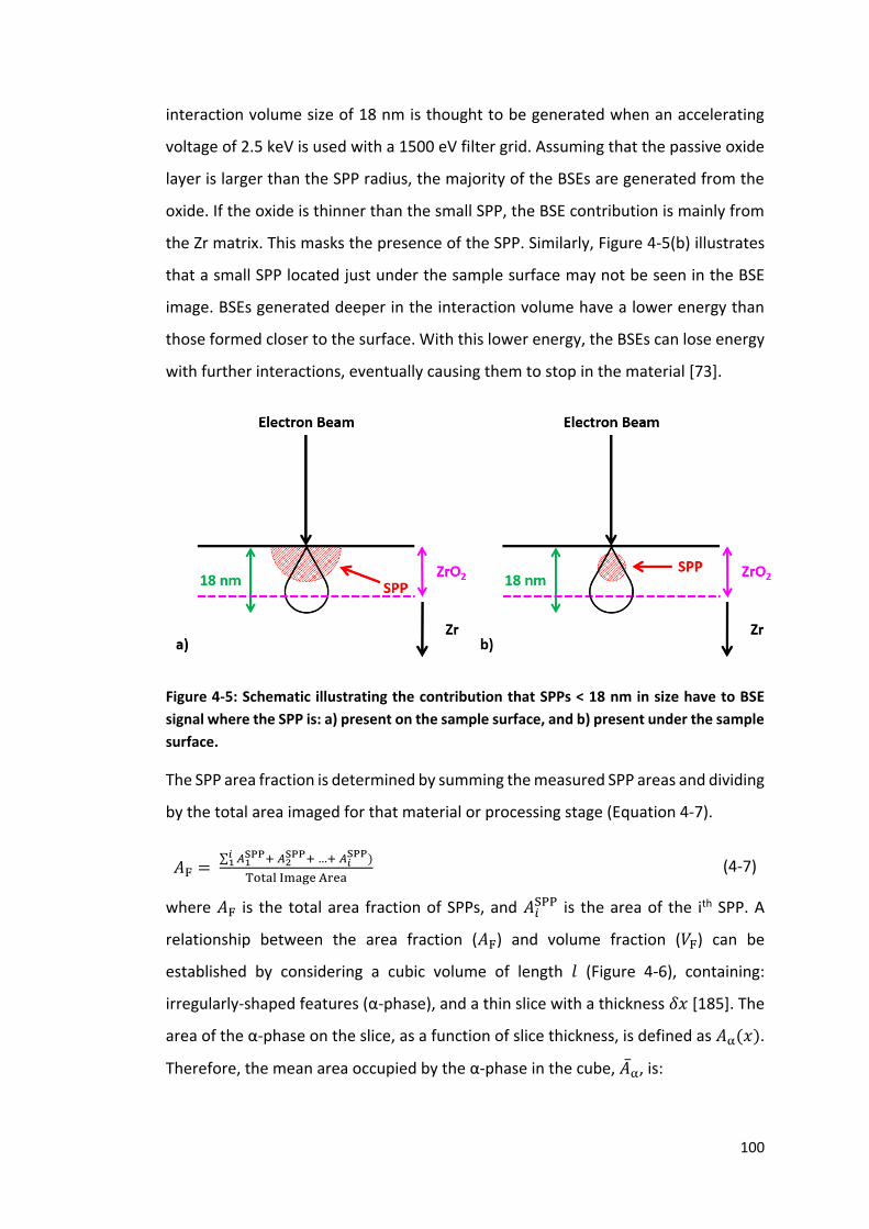
100

interaction volume size of 18 nm is thought to be generated when an accelerating

voltage of 2.5 keV is used with a 1500 eV filter grid. Assuming that the passive oxide

layer is larger than the SPP radius, the majority of the BSEs are generated from the

oxide. If the oxide is thinner than the small SPP, the BSE contribution is mainly from

the Zr matrix. This masks the presence of the SPP. Similarly, Figure 4-5(b) illustrates

that a small SPP located just under the sample surface may not be seen in the BSE

image. BSEs generated deeper in the interaction volume have a lower energy than

those formed closer to the surface. With this lower energy, the BSEs can lose energy

with further interactions, eventually causing them to stop in the material [73].

Figure 4-5: Schematic illustrating the contribution that SPPs < 18 nm in size have to BSE

signal where the SPP is: a) present on the sample surface, and b) present under the sample

surface.

The SPP area fraction is determined by summing the measured SPP areas and dividing

by the total area imaged for that material or processing stage (Equation 4-7).

𝐴F = ∑ 𝐴1

SPP+ 𝐴2SPP+ …+ 𝐴𝑖

SPP)𝑖1

Total Image Area (4-7)

where 𝐴F is the total area fraction of SPPs, and 𝐴𝑖SPP is the area of the ith SPP. A

relationship between the area fraction (𝐴F) and volume fraction (𝑉F) can be

established by considering a cubic volume of length 𝑙 (Figure 4-6), containing:

irregularly-shaped features (α-phase), and a thin slice with a thickness 𝛿𝑥 [185]. The

area of the α-phase on the slice, as a function of slice thickness, is defined as 𝐴α(𝑥).

Therefore, the mean area occupied by the α-phase in the cube, �̅�α, is:

101

�̅�α = 1

𝑙∫ 𝐴α(𝑥)

𝑙

0 𝑑𝑥 (4-8)

The α-phase volume in the thin slice is defined in Equation 4-9, and in the limit the

total α-phase volume is expressed in Equation 4-10.

𝛿𝑉α = 𝐴α(𝑥)𝛿𝑥 (4-9)

𝑉𝛼 = ∫ 𝐴𝛼(𝑥)𝑙

0 𝑑𝑥 (4-10)

Equation 4-8 and Equation 4-10 can be equated to form Equation 4-11. This is then

divided by the total volume, 𝑉T to form Equation 4-12.

𝑉α = 𝑙�̅�α (4-11)

𝑉α

𝑉T=

�̅�α

𝐴T (4-12)

Or for simplicity:

𝑉F = 𝐴F (4-13)

From this, it can be assumed that the SPP area fraction from the above particle

analysis is equivalent to the SPP volume fraction since the SPP measurements are

performed on a flat, two-dimensional area with minimal relief that is viewed with

electrons reflected from the sample surface [186]. In this case, the slice area is

equivalent to the image area and the slice thickness is the depth of the interaction

volume. In addition, the number of SPPs per unit volume (µm-3) is equivalent to the

SPP number per unit area (µm-2).

Figure 4-6: Cubic volume containing randomly oriented features, adapted from [185].

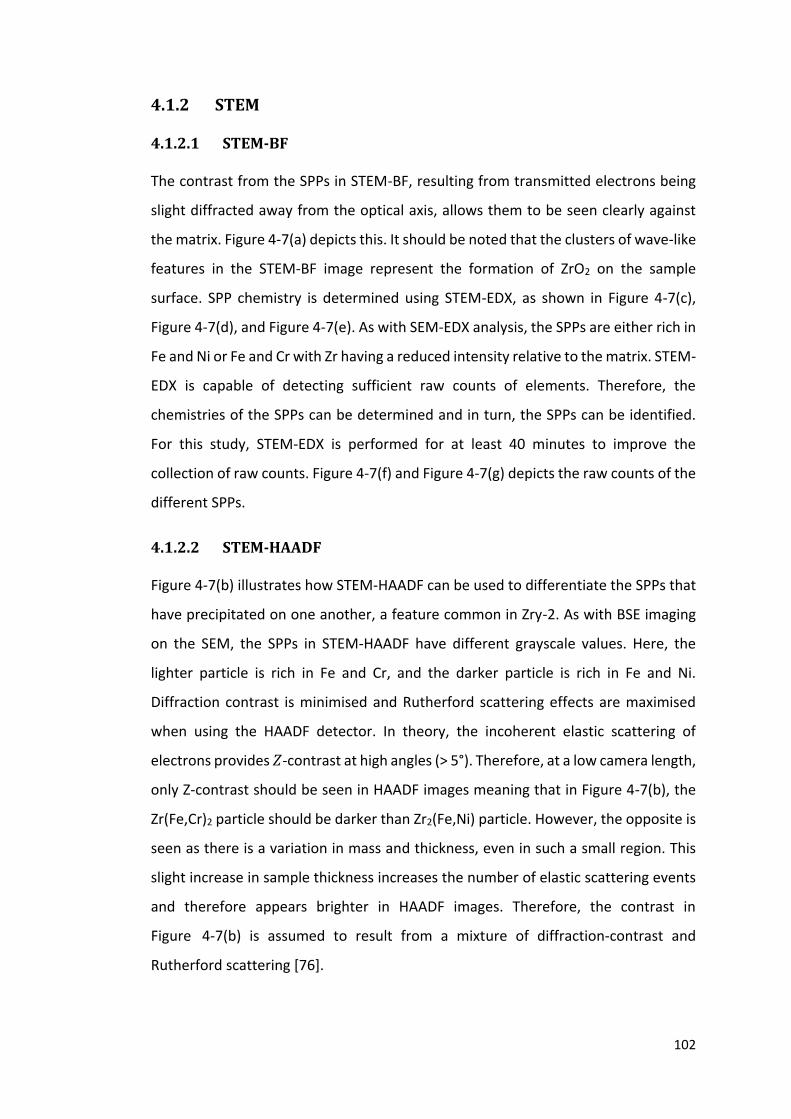
102

4.1.2 STEM

4.1.2.1 STEM-BF

The contrast from the SPPs in STEM-BF, resulting from transmitted electrons being

slight diffracted away from the optical axis, allows them to be seen clearly against

the matrix. Figure 4-7(a) depicts this. It should be noted that the clusters of wave-like

features in the STEM-BF image represent the formation of ZrO2 on the sample

surface. SPP chemistry is determined using STEM-EDX, as shown in Figure 4-7(c),

Figure 4-7(d), and Figure 4-7(e). As with SEM-EDX analysis, the SPPs are either rich in

Fe and Ni or Fe and Cr with Zr having a reduced intensity relative to the matrix. STEM-

EDX is capable of detecting sufficient raw counts of elements. Therefore, the

chemistries of the SPPs can be determined and in turn, the SPPs can be identified.

For this study, STEM-EDX is performed for at least 40 minutes to improve the

collection of raw counts. Figure 4-7(f) and Figure 4-7(g) depicts the raw counts of the

different SPPs.

4.1.2.2 STEM-HAADF

Figure 4-7(b) illustrates how STEM-HAADF can be used to differentiate the SPPs that

have precipitated on one another, a feature common in Zry-2. As with BSE imaging

on the SEM, the SPPs in STEM-HAADF have different grayscale values. Here, the

lighter particle is rich in Fe and Cr, and the darker particle is rich in Fe and Ni.

Diffraction contrast is minimised and Rutherford scattering effects are maximised

when using the HAADF detector. In theory, the incoherent elastic scattering of

electrons provides 𝑍-contrast at high angles (> 5°). Therefore, at a low camera length,

only Z-contrast should be seen in HAADF images meaning that in Figure 4-7(b), the

Zr(Fe,Cr)2 particle should be darker than Zr2(Fe,Ni) particle. However, the opposite is

seen as there is a variation in mass and thickness, even in such a small region. This

slight increase in sample thickness increases the number of elastic scattering events

and therefore appears brighter in HAADF images. Therefore, the contrast in

Figure 4-7(b) is assumed to result from a mixture of diffraction-contrast and

Rutherford scattering [76].

103

Figure 4-7: STEM analysis of SPPs in Zry-2 where electron imaging is performed using: a)

STEM-BF, and b) STEM-HAADF. Associated STEM-EDX is performed where: c) shows the Zr

map, d) shows the Cr/Ni map, and e) shows the Fe map. Raw counts of STEM-EDX are

shown in: f) for Cr-rich SPP, and g) for Ni-rich SPP.

Mass-thickness contrast adversely affect the imaging of SPPs smaller than that

observed in Figure 4-7(b). Figure 4-8 presents an example of this in β-quenched HiFi

supplied by Sandvik AB. The contribution of the matrix to mass-thickness contrast

masks the presence of the Zr(Fe,Cr)2 particles in the matrix that surround the larger

Zr2(Fe,Ni) particle in the STEM-HAADF image.

104

Figure 4-8: Mass-thickness contrast masking the presence of small Zr(Fe,Cr)2 particles

surrounding the larger Zr2(Fe,Ni) particle in industrially β-quenched HiFi.

Variations in mass and thickness over “large” distances are mainly observed in

electropolished foils. Perforation takes place during electropolishing, leading to the

formation of electron transparent regions. These regions are wedge-shaped from the

edge of the perforation to the foil periphery. Figure 4-9 illustrates this where the

grayscale value changes from the perforated area (darker) to the thicker region

(lighter) of the electropolished foil. This in turn adversely affects the contrast

observed on SPPs since SPPs furthest from the perforated region will have a greater

matrix contribution to the STEM-HAADF signal than the SPP closest to the perforated

region. Therefore, STEM-HAADF is not an ideal technique suitable for establishing

PSDs without consideration of the effects of variable thickness, which requires time-

consuming thickness measurements of the foil.

Figure 4-9: Thickness variation in electropolished foil.

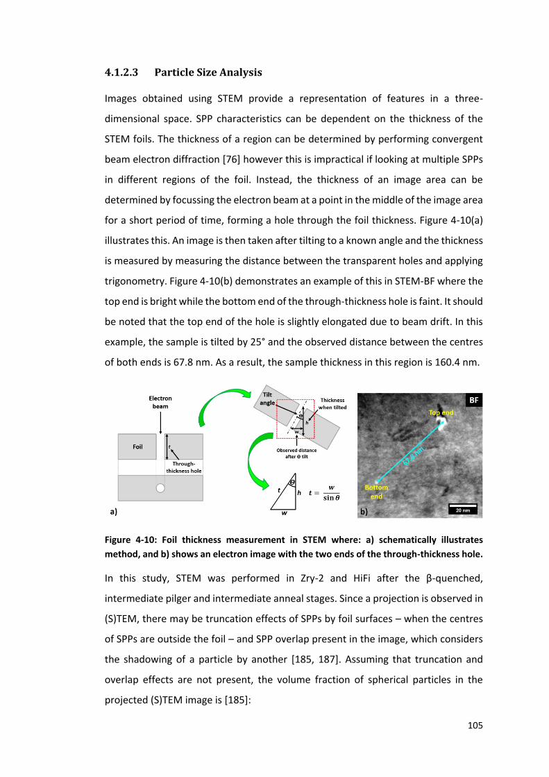
105

4.1.2.3 Particle Size Analysis

Images obtained using STEM provide a representation of features in a three-

dimensional space. SPP characteristics can be dependent on the thickness of the

STEM foils. The thickness of a region can be determined by performing convergent

beam electron diffraction [76] however this is impractical if looking at multiple SPPs

in different regions of the foil. Instead, the thickness of an image area can be

determined by focussing the electron beam at a point in the middle of the image area

for a short period of time, forming a hole through the foil thickness. Figure 4-10(a)

illustrates this. An image is then taken after tilting to a known angle and the thickness

is measured by measuring the distance between the transparent holes and applying

trigonometry. Figure 4-10(b) demonstrates an example of this in STEM-BF where the

top end is bright while the bottom end of the through-thickness hole is faint. It should

be noted that the top end of the hole is slightly elongated due to beam drift. In this

example, the sample is tilted by 25° and the observed distance between the centres

of both ends is 67.8 nm. As a result, the sample thickness in this region is 160.4 nm.

Figure 4-10: Foil thickness measurement in STEM where: a) schematically illustrates

method, and b) shows an electron image with the two ends of the through-thickness hole.

In this study, STEM was performed in Zry-2 and HiFi after the β-quenched,

intermediate pilger and intermediate anneal stages. Since a projection is observed in

(S)TEM, there may be truncation effects of SPPs by foil surfaces – when the centres

of SPPs are outside the foil – and SPP overlap present in the image, which considers

the shadowing of a particle by another [185, 187]. Assuming that truncation and

overlap effects are not present, the volume fraction of spherical particles in the

projected (S)TEM image is [185]:

106

𝑉F =2𝐴F�̅�true

3𝑡 (4-14)

where 𝐴F is the measured SPP area fraction, �̅�true is the mean value of the measured

SPP sizes, and 𝑡 is the foil thickness which is assumed to be even throughout the

image. Equation 4-15 is used instead if truncation is present, Equation 4-16 is used if

only SPP overlap is present (where 𝑡𝐷⁄ ≫ 1), and Equation 4-17 is used if both

truncation and SPP overlap is present [185].

𝑉F = 𝐴F (2𝐷true

2𝐷true+3𝑡) (4-15)

𝑉F = [−2 ln(1 − 𝐴F)] (𝐷true

𝑖

𝐷true𝑖 +3𝑡

) (4-16)

𝑉F = 𝐴F𝑖 (

𝐷true𝑖

𝐷true𝑖 +3𝑡

) (4-17)

where 𝐴F𝑖 is the area fraction of the ith SPP, and 𝐷true

𝑖 is the true size of the ith SPP.

Similarly, the number of SPPs per unit volume is described in Equation 4-18 if

truncation and overlap effects are not present, Equation 4-19 shows that for the

presence of truncation only, and Equation 4-20 shows that for SPP overlap only [185].

𝑁V = 𝑁A

𝑡 (4-18)

𝑁V = 𝑁A

(𝑡+�̅�true) (4-19)

𝑁V = 𝑁A+ 𝑀A

(𝑡+�̅�true) (4-20)

where 𝑁V is the number of SPPs per unit volume (particles/µm-3), 𝑁A is the SPP

number per unit area (particles/µm-2), and 𝑀A is the particle number per unit area

lost by overlap. SPPs were counted and their sizes were measured from the electron

images and EDX maps using ImageJ. Each image had their scale set and the particle

area was calculated. The area was then converted to the particle size, assuming it to

be spherical. This value is considered to be the “true” particle size since the real

diameter is imaged using STEM.

107

4.1.3 Comparison of SEM and STEM Characterization

4.1.3.1 Sample Preparation

As mentioned in Section 2.4, the time required for sample preparation, use of the

technique, and image analysis is different for both microscopy techniques. In this

study, the sample preparation for SEM specimens is different to those used in

previous studies [41, 66]. However, this SEM preparation technique (Section 3.2.1) is

still quicker, reproducible, and more reliable than that for producing TEM foils. Foil

production is time-consuming since care is required to produce a number of 100 µm

thick foils before electropolishing. The electropolishing process is not reliable since

the degree of perforation can change from foil to foil, which needs to be inspected

prior to use in the STEM.

4.1.3.2 Imaging

SEM imaging is performed on samples that are centimetres in size. Therefore, a large

number of SPPs can be imaged, generating reliable PSDs. Despite this, the resolution

limit of the SEM restricts the imaging of SPPs smaller than 18 nm. Nevertheless, a

field width of approximately 4 µm for each image is adequate enough to capture the

full range of particle sizes. However, the signal to noise (S/N) ratio for the ESB should

be suitable enough to provide adequate contrast between the SPPs. Thus, improving

the S/N increases the time required to generate BSE images. Figure 4-3 shows the

capabilities of the ESB detector, with a suitable S/N ratio, and windowless EDX

detector. Further, SPPs are crystallographically identified using EBSD. This is a quick

process and can be used over a large area.

Conversely, STEM imaging is performed on a limited sample size, restricting the

number of SPPs for the PSD. However, STEM is capable of producing atomic

resolution images. Thus, a higher density of SPPs smaller than 18 nm can be imaged

and identified. Electron transparent regions in STEMs that operate at 200 keV are

usually less than approximately 100 nm [76]. However, as seen in Figure 4-9, pits are

usually observed. This is caused by a difference in electrochemistry between the

matrix and SPP where the matrix polishes at a quicker rate than the SPP. If the matrix

becomes too thin, it can no longer hold the SPP in place, causing the SPP to drop out

108

from the matrix. This is prominent in the amorphous regions or regions where the

thickness is less than 100 nm but not frequently seen in thicker regions. Therefore,

SPPs in STEM foils are not limited to a maximum size of 100 nm but can be larger

when imaged in the thicker regions. Furthermore, very small particles, like those seen

in Figure 4-8, can be identified in the thickness of the matrix. This is one of the

advantages of using (S)TEM where the transmitted electrons provide information

throughout the foil thickness. STEM-BF imaging of SPPs is quicker since the S/N ratio

does not require adjustment. Since STEM-BF imaging cannot differentiate the SPPs,

STEM-EDX is performed for each image. This can be a quick and simple procedure if

producing EDX maps though it can be time consuming if a large number of raw counts

are required to not only identify the correct SPP type and allow for solute ratio

analysis. SPPs can be crystallographically identified using diffraction in the

conventional TEM. This is a time consuming process since this requires knowledge of

diffraction pattern zone axes and multiple adjustments when tilting the sample to

correctly image the diffraction pattern. In addition, since the SPPs are generally

located in thick regions of the foil, the SPPs provide a very small contribution to the

diffraction pattern. Figure 4-11 illustrates this for the attempted diffraction pattern

of Zr(Fe,Cr)2 in Zry-2 where the diffraction spots are associated to the Zr basal plane.

Figure 4-11: Diffraction pattern of basal plane in Zry-2.

4.1.3.3 SPP Characterization Analysis

Figure 4-12 shows a comparison of the PSDs and cumulative number density (which

includes all SPPs larger than the considered particle size) graphs obtained from both

109

SEM and STEM for both SPP types in HiFi at the intermediate anneal stage of

thermomechanical processing. The error bars on the pink histogram bars and blue

histogram bars show the standard error of the number density of both SPP types

obtained using SEM and STEM imaging respectively. The error bar on the horizontal

red line and on the horizontal orange line are the standard errors of the mean size

for both SPP types obtained using SEM and STEM imaging respectively. The class

width was determined using Equation 4-6 from Gros and Wadier [107]. Here, the

SPPs in the SEM were imaged in an approximate area of 325 µm2 and the SPPs imaged

in STEM covered an area of approximately 90 µm2. It should be noted that the SPP

measurements in STEM were performed at least 5 µm from perforation. This is due

to the fact that after electropolishing, large SPPs have the tendency to drop from the

matrix when located in thin regions surrounding the perforation. As a result, the foil

thickness in the regions of interest was approximately 500 nm. With the relatively

large particles present, it can be assumed that no truncation or overlap is present.

Therefore, SPP number density using STEM was determined using Equation 4-18.

Figure 4-12 shows that SPP number densities observed in the SEM are generally

lower than that from STEM. From Figure 4-12(b) and Figure 4-12(d), a high number

density of SPPs smaller than 150 nm in size is observed where STEM demonstrates

the number density of Zr(Fe,Cr)2 particles and Zr2(Fe,Ni) particles being 0.42 µm-3 and

0.28 µm-3 respectively while that observed using SEM shows a number density of

0.26 µm-3 and 0.16 µm-3 respectively. This illustrates the advantages of using STEM

with regards to this technique’s higher spatial resolution. Then again, the SEM

measurements identify SPPs smaller than that measured using STEM. Table 4-1

illustrates this. Further, the SEM identifies larger SPPs than that identified in STEM.

Specimens used in SEM do not have the same restrictions that STEM specimens have

and therefore, there is no upper limit to measured feature size in SEM. On the other

hand, STEM-EDX measurements further away from the perforated region could

reveal larger SPPs present in the foil though the foil thickness would be difficult to

measure. The mean Zr2(Fe,Ni) size measured using SEM is larger than obtained from

STEM. This is expected since larger particles are readily observed in SEM than that in

STEM. On the other hand, the mean Zr(Fe,Cr)2 size is similar with that obtained using

110

STEM being slightly larger. Nonetheless, the reliability of the PSDs obtained using

STEM is questionable since only a total of 61 SPPs were counted while 285 SPPs were

observed in SEM. The difference in total image area from both techniques

contributes to this where STEM is limited with sample size. This could lead to the

differences in SPP number density and volume fraction obtained using both

techniques. The SPP number density obtained using SEM is lower than that obtained

from STEM. This could result from the fact that STEM imaging uses transmitted

electrons and therefore is capable of identifying SPPs through the thickness of the

sample while SEM imaging uses reflected electrons that provide information at the

specimen surface. Conversely, the volume fraction of both SPP types is larger when

imaged using SEM than that obtained from STEM imaging. These differences most

likely originate from the SPP volume fraction defined by Equation 4-14. This term is

dependent on the thickness of (S)TEM foils where the thickness associated to the

STEM images at this stage is an average value. Variations in foil thickness between

the image extremities can have a significant impact on the contribution that the SPP

has on volume fraction. As a result, the volume fraction obtained from STEM could

be an underestimate to the actual volume fraction.

111

Figure 4-12: Comparison of PSDs and cumulative size distributions in HiFi at the

intermediate anneal stage using SEM and STEM where: a) shows the Zr(Fe,Cr)2 PSD, b)

shows the Zr(Fe,Cr)2 cumulative size distribution, c) shows Zr2(Fe,Ni) PSD, and d) shows the

Zr2(Fe,Ni) cumulative size distribution. The error bars on the pink histogram bars and blue

histogram bars show the standard error of the number density of both SPP types obtained

using SEM and STEM imaging respectively. The error bar on the horizontal red line and on

the horizontal orange line are the standard errors of the mean size for both SPP types

obtained using SEM and STEM imaging respectively. The class width was determined using

Equation 4-6 from Gros and Wadier [107].

Table 4-1: SPPs characteristics of Zr(Fe,Cr)2 and Zr2(Fe,Ni) in HiFi at the intermediate anneal

stage, obtained using SEM and STEM.

Zr(Fe,Cr)2 Zr2(Fe,Ni)

SEM STEM SEM STEM

Min SPP size (nm)

54.9 71.0 79.2 114.0

Max SPP size (nm)

377.3 354.6 494.1 315.2

Mean SPP size (nm)

167.6 175.8 213.8 195.3

SPP Number

135 31 150 30

Number density (µm-3)

0.44 0.70 0.49 0.66

Volume Fraction

0.005 0.003 0.009 0.003

112

4.2 DSC

DSC was performed on the industrially β-quenched Zry-2 and HiFi to show how valid

this technique is for SPP characterization. Figure 4-13 illustrates the DSC

measurements (red line) for β-quenched Zry-2. Here, there are two endothermic

peaks between the temperatures of 800 °C and 1000 °C which are of interest. The

higher temperature peak, labelled as 2, corresponds to the α-Zr to β-Zr phase

transformation. The peak identified as 1 corresponds to the dissolution of the SPPs.

Since there are two separate SPP types present in Zry-2, there should be two

endothermic peaks corresponding to their respective dissolution. Since only one

peak is present here, the SPP peaks cannot be separated via a deconvolution of

enthalpic peaks since the dissolution temperatures are too close together. The

presence of the different SPP types can be confirmed using the differential of the DSC

measurements (DDSC). This is shown with a blue line. The peaks at 822 °C and 833 °C

relate to the dissolution temperatures of the SPPs. It should be noted that the

changes in enthalpy from room temperature to approximately 800 °C can be

attributed to the formation of ZrO2 on the sample surface.

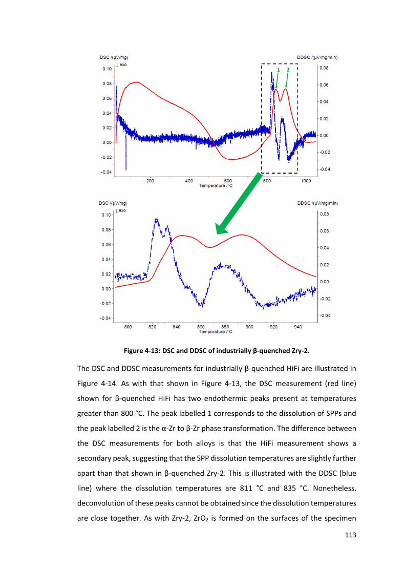
113

Figure 4-13: DSC and DDSC of industrially β-quenched Zry-2.

The DSC and DDSC measurements for industrially β-quenched HiFi are illustrated in

Figure 4-14. As with that shown in Figure 4-13, the DSC measurement (red line)

shown for β-quenched HiFi has two endothermic peaks present at temperatures

greater than 800 °C. The peak labelled 1 corresponds to the dissolution of SPPs and

the peak labelled 2 is the α-Zr to β-Zr phase transformation. The difference between

the DSC measurements for both alloys is that the HiFi measurement shows a

secondary peak, suggesting that the SPP dissolution temperatures are slightly further

apart than that shown in β-quenched Zry-2. This is illustrated with the DDSC (blue

line) where the dissolution temperatures are 811 °C and 835 °C. Nonetheless,

deconvolution of these peaks cannot be obtained since the dissolution temperatures

are close together. As with Zry-2, ZrO2 is formed on the surfaces of the specimen

114

during the DSC measurement during the heating stage from room temperature to

800 °C.

Figure 4-14: DSC and DDSC of industrially β-quenched HiFi.

The DSC is capable of measuring the enthalpy of the dissolution of separate SPPs and

distinguishing the different temperatures at which this take place. However, since

the dissolution temperatures are within 25 °C of each other, the SPP dissolution

peaks cannot be differentiated and therefore, the DSC is not a suitable technique for

tracking SPP precipitation kinetics.

115

4.3 TEP

Figure 4-15 demonstrates TEP measurements of Zry-2 and HiFi, β-quenched from

1150 °C followed by isothermal heat treatments at either 600 °C or 700 °C. These are

measured relative to a β-quenched reference. The error bars at each data point show

the standard error of the mean of all TEP measurements produced at each heat

treatment condition. In all cases, there is an increase in relative TEP value before it

plateaus. This trend is consistent with a study performed by Loucif et al. on the TEP

evolution in α-quenched Zry-2, heat treated in the temperature range of 450 °C to

600 °C (Figure 2-12) [94]. However, the TEP at 600 °C for Zry-2 in this study reaches

a plateau at longer heat treatment times than that seen by Loucif et al. This is due to

the fact that Loucif et al. performed their water quench process from 805 °C. As

shown in Figure 4-13, SPP dissolution temperatures are higher than 805 °C.

Therefore, the SPPs are not fully dissolved and matrix is not fully supersaturated in

solute. Subsequent heat treatments would then be shorter in time in order to

complete the precipitation process. In addition, in this study the maximum TEP at

600 °C for Zry-2 is larger than that observed in the study performed by Loucif et al.

This is attributed to the supersaturation obtained in the β-quench process performed

in this study. The β-quenched reference has minimum SPP formation due to the large

cooling rate and therefore a higher solute concentration than that obtained from α-

quenching from 805 °C [99]. Heat treatments following β-quenching lead to larger

changes in solute concentration in the matrix and therefore larger changes in TEP are

observed. This also explains the difference in maximum TEP obtained between Zry-2

and HiFi for the same temperature. Since HiFi has a higher Fe content than Zry-2,

there is more Fe in solution which then precipitates out. This larger reduction in Fe

concentration during the heat treatments from the β-quenched state to the fully

precipitated state leads to a more positive TEP. It should be noted that TEP is also

sensitive to changes in the concentration of specific solutes in the matrix. However,

the solutes of interest (Fe, Cr, and Ni) have electron arrangements that lead to similar

effects on TEP for each element, and all influence TEP in the same sense [91].

116

Figure 4-15: Variation of TEP against isothermal heat treatment time of β-quenched Zry-2

and HiFi relative to its β-quenched reference where: a) shows β-quenched Zry-2 heat

treated at 600 °C, b) shows β-quenched Zry-2 heat treated at 700 °C, c) shows β-quenched

HiFi heat treated at 600 °C, and d) shows β-quenched HiFi heat treated at 700 °C. The error

bars at each data point show the standard error of the mean of all TEP measurements

produced at each heat treatment condition.

Figure 4-15(a) illustrates that when β-quenched Zry-2 is isothermally heat treated at

600 °C, the precipitation process is complete, or the equilibrium SPP volume fraction

is attained, after approximately 20 hr. On the other hand, Figure 4-15(c) shows that

the precipitation process in β-quenched HiFi for the same heat treatment is complete

after 10 hr. This suggests that the increased Fe content in HiFi leads to accelerated

precipitation kinetics. This is confirmed, though to a lesser extent, by Loucif et al.

where the authors compared the time taken to reach 90 % of TEP variation in

isothermally heat treated Zr-Fe alloys with varying Fe content [94]. The increased Fe

content leads to accelerated SPP formation and therefore an accelerated reduction

in solute concentration with increased heat treatment time. This effect is similarly

shown between Figure 4-15(b) and Figure 4-15(d) when both β-quenched Zry-2 and

HiFi are isothermally heat treated at 700 °C.

117

Accelerated precipitation is also seen when the isothermal heat treatment

temperature increases. Figure 4-15(b) shows that the precipitation process in β-

quenched Zry-2 heat treated at 700 °C is complete after 2 hr and Figure 4-15(d)

illustrates that β-quenched HiFi completes the precipitation process after 1 hr when

heat treated at 700 °C. With increasing temperature, the diffusion of solutes such as

Fe, Cr, and Ni increases in α-Zr. This in turn increases the SPP growth rate and thus

reduces the solute concentration in the matrix quicker than when the materials are

heat treated at 600 °C [121, 123]. As a result, the equilibrium SPP volume fraction is

attained sooner.

TEP has the potential of tracking the change in solute concentration with processing

stages, especially when heat treatments are applied to the materials. The change in

solute concentration is linked to the change in SPP volume fraction. From this, the

time for the completion of precipitation, or the time at which particle coarsening

takes place, can be determined. Therefore, TEP is a suitable technique for tracking

the overall precipitation kinetics of SPPs.

4.4 Summary

This chapter introduced the experimental techniques that have been used to attempt

SPP characterization in Zry-2 and HiFi. The capabilities of the aforementioned

techniques’ is presented in Table 4-2.

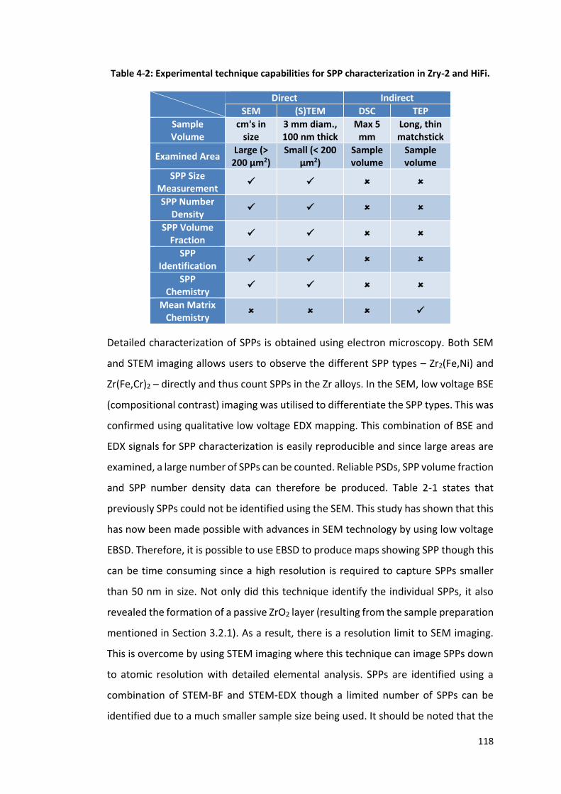
118

Table 4-2: Experimental technique capabilities for SPP characterization in Zry-2 and HiFi.

Direct Indirect

SEM (S)TEM DSC TEP

Sample Volume

cm's in size

3 mm diam., 100 nm thick

Max 5 mm

Long, thin matchstick

Examined Area Large (>

200 µm2) Small (< 200

µm2) Sample volume

Sample volume

SPP Size Measurement

SPP Number Density

SPP Volume Fraction

SPP Identification

SPP Chemistry

Mean Matrix Chemistry

Detailed characterization of SPPs is obtained using electron microscopy. Both SEM

and STEM imaging allows users to observe the different SPP types – Zr2(Fe,Ni) and

Zr(Fe,Cr)2 – directly and thus count SPPs in the Zr alloys. In the SEM, low voltage BSE

(compositional contrast) imaging was utilised to differentiate the SPP types. This was

confirmed using qualitative low voltage EDX mapping. This combination of BSE and

EDX signals for SPP characterization is easily reproducible and since large areas are

examined, a large number of SPPs can be counted. Reliable PSDs, SPP volume fraction

and SPP number density data can therefore be produced. Table 2-1 states that

previously SPPs could not be identified using the SEM. This study has shown that this

has now been made possible with advances in SEM technology by using low voltage

EBSD. Therefore, it is possible to use EBSD to produce maps showing SPP though this

can be time consuming since a high resolution is required to capture SPPs smaller

than 50 nm in size. Not only did this technique identify the individual SPPs, it also

revealed the formation of a passive ZrO2 layer (resulting from the sample preparation

mentioned in Section 3.2.1). As a result, there is a resolution limit to SEM imaging.

This is overcome by using STEM imaging where this technique can image SPPs down

to atomic resolution with detailed elemental analysis. SPPs are identified using a

combination of STEM-BF and STEM-EDX though a limited number of SPPs can be

identified due to a much smaller sample size being used. It should be noted that the

119

reduced number density of SPPs in STEM imaging can be related to the fact that STEM

sample preparation (Section 3.2.2) leads to SPPs dropping out of the matrix close to

the electron-transparent region. In addition to this, extensive analysis is required to

characterize SPPs using STEM. Since images are seen through the foil thickness, SPP

truncation and overlap have to be taken into consideration. Furthermore, foil

thickness measurements are necessary to determine SPP volume fraction and

number density. Nonetheless, PSDs, SPP volume fraction and SPP number density

data can be produced though this is less reliable than that produced using SEM

imaging. Finally, matrix chemistry could be obtained using EDX in both SEM and STEM

though the matrix thickness was too large to obtain any relevant information.

Nevertheless, electron microscopy can be used to characterize SPPs in Zry-2 and HiFi.

This is illustrated further in Chapter 5 where SPP characterization is performed at

each thermomechanical processing stage from the β-quench stage down to the final

product.

DSC and TEP are both indirect techniques and thus SPPs cannot be observed.

However, with multiple sample runs using either technique can provide information

that can be tracked. DSC had been identified to track the SPP volume fraction with

further heat treatments by considering the area under the enthalpy peaks relating to

SPP dissolution. Experiments using β-quenched Zry-2 and HiFi (supplied by Sandvik

AB) easily show the α-Zr to β-Zr phase transformation (point 2 in Figure 4-13 and

Figure 4-14) and an additional enthalpy peak at a slightly lower temperature (relating

to SPP dissolution). However, since the dissolution temperatures for Zr2(Fe,Ni) and

Zr(Fe,Cr)2 are too close together, their respective enthalpy peaks cannot be

distinguished and thus tracking the evolution of SPP volume fraction was not

possible. Therefore, the DSC is not a suitable technique for tracking SPP precipitation

kinetics.

TEP had been identified as a technique of tracking the solute concentration in the

matrix with further heat treatments. The change in solute concentration is inversely

proportional to the change in SPP volume fraction (where decreasing solute

concentration in the matrix shows an increase in SPP volume fraction). TEP

measurements of heat treated material were made possible if they were relative to

120

a reference (β-quenched material with a quenching rate of 1500 °C/s). At heat

treatment temperatures of 600 °C and 700 °C, TEP measurements (Figure 4-15) show

that solute concentration in the matrix reaches a plateau. At this point, the volume

fraction is at a constant value and the precipitation process is complete (SPP

coarsening is dominant). The onset of SPP coarsening is the point at which the

plateau starts. TEP measurements at the plateau for Zry-2 are smaller than that for

HiFi since fewer solutes are precipitating out of the matrix (Zry-2 has a lower solute

concentration in the β-quenched material). Further, the onset of coarsening is

started earlier at 700 °C for both alloys due to accelerated kinetics. However, the

SPPs cannot be distinguished using TEP and thus this technique is presenting the

combined kinetics of both SPP types. Nonetheless, TEP is a technique that is suitable

for tracking the overall SPP precipitation kinetics. The results from the TEP can be

coupled with SEM and STEM imaging, providing in-depth analysis of the behaviour of

both SPPs types during these heat treatments. This analysis will be used to calibrate

a precipitation kinetics model, described in Chapter 6.

121

5 Evolution of SPP Characteristics throughout

Thermomechanical Processing

SEM and STEM were implemented to describe SPP evolution throughout

thermomechanical processing of Zry-2 and HiFi cladding material. Firstly, a

comparison of SPP characteristics in both alloys are compared at the same processing

stage. Thereafter, SPP characterization is performed at all stages of

thermomechanical processing from the β-quench stage to the final anneal stage.

Thermomechanical processing of the cladding tubes was performed by Sandvik AB

and the material used in this study was taken directly after each stage. This allowed

for the independent effects of hot work, cold pilgering, and annealing on SPP

characteristics to be investigated.

5.1 SPP Characteristics in Zircaloy-2 and HiFi

Comparisons between the SPP characteristics in Zry-2 and HiFi are performed by

analysing the particle distributions at the final anneal stage using SEM imaging with

a total image area of 325 µm2 examined for each alloy. The error bars on the pink

histogram bars and blue histogram bars show the standard error of the number

density of both SPP types in Zry-2 and HiFi respectively. The error bar on the

horizontal red line and on the horizontal orange line are the standard errors of the

mean size for both SPP types in Zry-2 and HiFi respectively. The class width was

determined using Equation 4-6 from Gros and Wadier [107]. Figure 5-1 illustrates the

SPP and cumulative density distributions (which includes all SPPs larger than the

considered particle size) of both SPP types in Zry-2 and HiFi where the mean sizes of

both SPP types in HiFi are larger than the respective SPP mean sizes in Zry-2.

122

Figure 5-1: SPP size distributions of Zry-2 and HiFi for: a) Zr(Fe,Cr)2, and b) Zr2(Fe,Ni) &

cumulative density distributions for both alloys for: c) Zr(Fe,Cr)2, and d) Zr2(Fe,Ni). The

mean particle size of both SPP types are shown as vertical lines. SPP imaging is performed

using the SEM.

From Figure 5-1(a), Zry-2 has a larger number density of Zr(Fe,Cr)2 particles smaller

than 50 nm in size while HiFi seems to have a larger number density of Zr(Fe,Cr)2

particles larger than 100 nm in size. The distribution of the Zr2(Fe,Ni) particles on the

other hand, in Figure 5-1(b), looks similar for both alloys though as with the Zr(Fe,Cr)2

particles, Zry-2 has a larger number density of Zr2(Fe,Ni) particles smaller than

100 nm. These trends are illustrated in the cumulative density graphs shown in

Figure 5-1(c) and Figure 5-1(d). The total SPP number density can be examined using

the cumulative number density graphs. At this processing stage, Zry-2 has a higher

total number density of Zr(Fe,Cr)2 particles and a similar total number density of

Zr2(Fe,Ni) particles to that in HiFi. The higher number density of Zr(Fe,Cr)2 particles

smaller than 50 nm in Zry-2 is illustrated by the steeper gradient in comparison to

that for HiFi, as illustrated in Figure 5-1(c). The same is observed in the behaviour of

Zr2(Fe,Ni) particles in Figure 5-1(d) where a slightly steeper gradient for Zry-2 shows

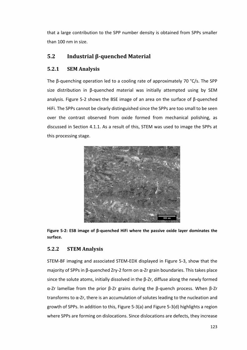
123

that a large contribution to the SPP number density is obtained from SPPs smaller

than 100 nm in size.

5.2 Industrial β-quenched Material

5.2.1 SEM Analysis

The β-quenching operation led to a cooling rate of approximately 70 °C/s. The SPP

size distribution in β-quenched material was initially attempted using by SEM

analysis. Figure 5-2 shows the BSE image of an area on the surface of β-quenched

HiFi. The SPPs cannot be clearly distinguished since the SPPs are too small to be seen

over the contrast observed from oxide formed from mechanical polishing, as

discussed in Section 4.1.1. As a result of this, STEM was used to image the SPPs at

this processing stage.

Figure 5-2: ESB image of β-quenched HiFi where the passive oxide layer dominates the

surface.

5.2.2 STEM Analysis

STEM-BF imaging and associated STEM-EDX displayed in Figure 5-3, show that the

majority of SPPs in β-quenched Zry-2 form on α-Zr grain boundaries. This takes place

since the solute atoms, initially dissolved in the β-Zr, diffuse along the newly formed

α-Zr lamellae from the prior β-Zr grains during the β-quench process. When β-Zr

transforms to α-Zr, there is an accumulation of solutes leading to the nucleation and

growth of SPPs. In addition to this, Figure 5-3(a) and Figure 5-3(d) highlights a region

where SPPs are forming on dislocations. Since dislocations are defects, they increase

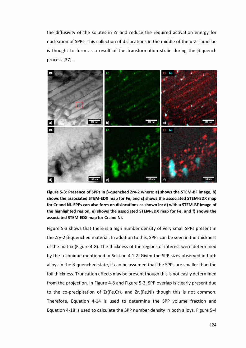
124

the diffusivity of the solutes in Zr and reduce the required activation energy for

nucleation of SPPs. This collection of dislocations in the middle of the α-Zr lamellae

is thought to form as a result of the transformation strain during the β-quench

process [37].

Figure 5-3: Presence of SPPs in β-quenched Zry-2 where: a) shows the STEM-BF image, b)

shows the associated STEM-EDX map for Fe, and c) shows the associated STEM-EDX map

for Cr and Ni. SPPs can also form on dislocations as shown in: d) with a STEM-BF image of

the highlighted region, e) shows the associated STEM-EDX map for Fe, and f) shows the

associated STEM-EDX map for Cr and Ni.

Figure 5-3 shows that there is a high number density of very small SPPs present in

the Zry-2 β-quenched material. In addition to this, SPPs can be seen in the thickness

of the matrix (Figure 4-8). The thickness of the regions of interest were determined

by the technique mentioned in Section 4.1.2. Given the SPP sizes observed in both

alloys in the β-quenched state, it can be assumed that the SPPs are smaller than the

foil thickness. Truncation effects may be present though this is not easily determined

from the projection. In Figure 4-8 and Figure 5-3, SPP overlap is clearly present due

to the co-precipitation of Zr(Fe,Cr)2 and Zr2(Fe,Ni) though this is not common.

Therefore, Equation 4-14 is used to determine the SPP volume fraction and

Equation 4-18 is used to calculate the SPP number density in both alloys. Figure 5-4

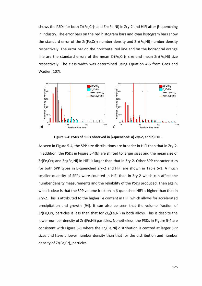
125

shows the PSDs for both Zr(Fe,Cr)2 and Zr2(Fe,Ni) in Zry-2 and HiFi after β-quenching

in industry. The error bars on the red histogram bars and cyan histogram bars show

the standard error of the Zr(Fe,Cr)2 number density and Zr2(Fe,Ni) number density

respectively. The error bar on the horizontal red line and on the horizontal orange

line are the standard errors of the mean Zr(Fe,Cr)2 size and mean Zr2(Fe,Ni) size

respectively. The class width was determined using Equation 4-6 from Gros and

Wadier [107].

Figure 5-4: PSDs of SPPs observed in β-quenched: a) Zry-2, and b) HiFi.

As seen in Figure 5-4, the SPP size distributions are broader in HiFi than that in Zry-2.

In addition, the PSDs in Figure 5-4(b) are shifted to larger sizes and the mean size of

Zr(Fe,Cr)2 and Zr2(Fe,Ni) in HiFi is larger than that in Zry-2. Other SPP characteristics

for both SPP types in β-quenched Zry-2 and HiFi are shown in Table 5-1. A much

smaller quantity of SPPs were counted in HiFi than in Zry-2 which can affect the

number density measurements and the reliability of the PSDs produced. Then again,

what is clear is that the SPP volume fraction in β-quenched HiFi is higher than that in

Zry-2. This is attributed to the higher Fe content in HiFi which allows for accelerated

precipitation and growth [94]. It can also be seen that the volume fraction of

Zr(Fe,Cr)2 particles is less than that for Zr2(Fe,Ni) in both alloys. This is despite the

lower number density of Zr2(Fe,Ni) particles. Nonetheless, the PSDs in Figure 5-4 are

consistent with Figure 5-1 where the Zr2(Fe,Ni) distribution is centred at larger SPP

sizes and have a lower number density than that for the distribution and number

density of Zr(Fe,Cr)2 particles.

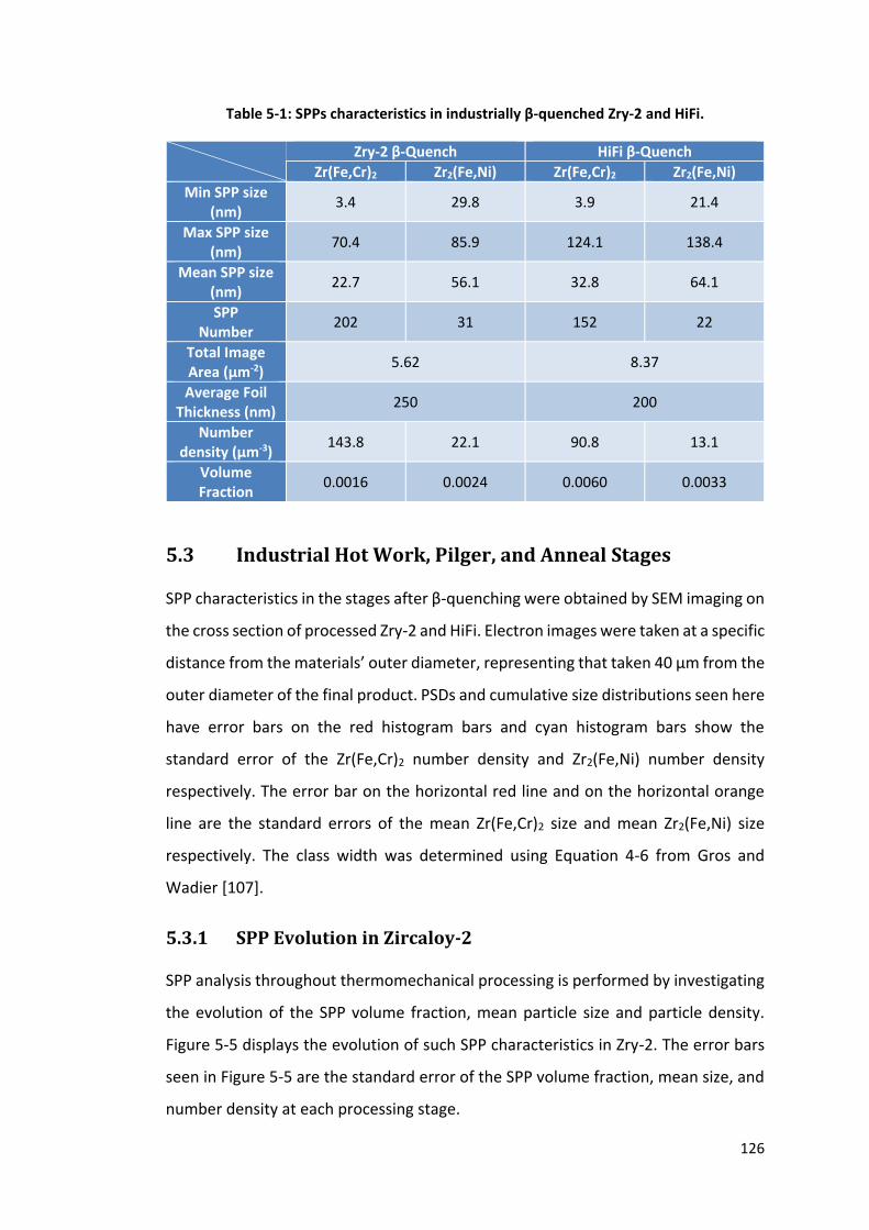
126

Table 5-1: SPPs characteristics in industrially β-quenched Zry-2 and HiFi.

Zry-2 β-Quench HiFi β-Quench

Zr(Fe,Cr)2 Zr2(Fe,Ni) Zr(Fe,Cr)2 Zr2(Fe,Ni)

Min SPP size (nm)

3.4 29.8 3.9 21.4

Max SPP size (nm)

70.4 85.9 124.1 138.4

Mean SPP size (nm)

22.7 56.1 32.8 64.1

SPP Number

202 31 152 22

Total Image Area (μm-2)

5.62 8.37

Average Foil Thickness (nm)

250 200

Number density (µm-3)

143.8 22.1 90.8 13.1

Volume Fraction

0.0016 0.0024 0.0060 0.0033

5.3 Industrial Hot Work, Pilger, and Anneal Stages

SPP characteristics in the stages after β-quenching were obtained by SEM imaging on

the cross section of processed Zry-2 and HiFi. Electron images were taken at a specific

distance from the materials’ outer diameter, representing that taken 40 µm from the

outer diameter of the final product. PSDs and cumulative size distributions seen here

have error bars on the red histogram bars and cyan histogram bars show the

standard error of the Zr(Fe,Cr)2 number density and Zr2(Fe,Ni) number density

respectively. The error bar on the horizontal red line and on the horizontal orange

line are the standard errors of the mean Zr(Fe,Cr)2 size and mean Zr2(Fe,Ni) size

respectively. The class width was determined using Equation 4-6 from Gros and

Wadier [107].

5.3.1 SPP Evolution in Zircaloy-2

SPP analysis throughout thermomechanical processing is performed by investigating

the evolution of the SPP volume fraction, mean particle size and particle density.

Figure 5-5 displays the evolution of such SPP characteristics in Zry-2. The error bars

seen in Figure 5-5 are the standard error of the SPP volume fraction, mean size, and

number density at each processing stage.

127

Figure 5-5: Evolution of SPP characteristics throughout thermomechanical processing in

Zry-2 cladding material at the β-quench stage (using STEM imaging), and from the hot work

stage to the final stage (using SEM imaging) where: a) shows SPP volume fraction, b) shows

mean SPP size, and c) shows SPP number density (axis breaks are used to illustrate the high

SPP number density present at the β-quench stage).

128

The total SPP volume fraction increases from 0.0040 to 0.0086 between the β-quench

stage to hot work stage. Thereafter, the total SPP volume fraction decreases slightly

from the hot work stage to the final product, from 0.0086 to 0.0069 though this

seems to be within error. SPP coarsening is thought to be taking place between the

hot work and final anneal stages since the volume fraction is relatively constant. This

is consistent with the TEP analysis in Section 4.3. After the hot work stage, the total

volume fraction of both SPP types decreases slightly from the intermediate pilger to

final anneal stage though these differences are within the error measured in SPP

measurements. The volume fraction of Zr2(Fe,Ni) generally decreases from the hot

work stage (0.0057) to the final anneal stage (0.0039) while the volume fraction of

Zr(Fe,Cr)2 particles is relatively constant throughout processing.

The mean particle size of both SPP types increases drastically from the β-quench

stage to the hot work stage. This suggests that significant SPP growth has taken place

at the hot work stage. Figure 5-6(a) illustrates this where the PSDs of both SPP types

are shifted to larger sizes relative to that seen in Figure 5-4(a). Thereafter, the mean

particle size decreases slightly from the hot work stage to the final anneal stage from

an overall mean size of 145.1 nm to 119.5 nm. However, it can be seen that the mean

particle size decreases with each pilger step and increases with each anneal step. The

decrease in mean particle size after pilgering is illustrated further by examining the

PSDs and cumulative number densities of SPPs at the hot work stage, depicted in

Figure 5-6(a) and Figure 5-6(b), and intermediate pilger stage, shown in Figure 5-6(c)

and Figure 5-6(d). A higher number density of smaller particles is present in the

intermediate pilger stage. Figure 5-6(c) illustrates this for both SPP types since the

PSDs are skewed to smaller SPP sizes. This is also confirmed in Figure 5-6(d) through

the examination of the cumulative number density graphs where a sharper reduction

in number density is seen in the intermediate pilger stage for both SPP types at

particle sizes smaller than 75 nm. The increase in SPP size during annealing is

analysed by comparing the PSDs and cumulative density graphs obtained from the

intermediate pilger and intermediate anneal stages. Figure 5-6(e) and Figure 5-6(f)

illustrates this for the intermediate anneal stage. Figure 5-6(e) shows that the size

distribution of Zr(Fe,Cr)2 particles skews a little to larger particle sizes in comparison

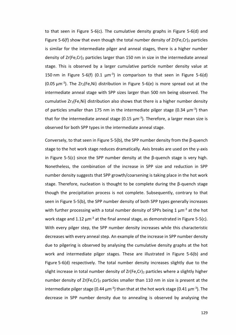
129

to that seen in Figure 5-6(c). The cumulative density graphs in Figure 5-6(d) and

Figure 5-6(f) show that even though the total number density of Zr(Fe,Cr)2 particles

is similar for the intermediate pilger and anneal stages, there is a higher number

density of Zr(Fe,Cr)2 particles larger than 150 nm in size in the intermediate anneal

stage. This is observed by a larger cumulative particle number density value at

150 nm in Figure 5-6(f) (0.1 µm-3) in comparison to that seen in Figure 5-6(d)

(0.05 µm-3). The Zr2(Fe,Ni) distribution in Figure 5-6(e) is more spread out at the

intermediate anneal stage with SPP sizes larger than 500 nm being observed. The

cumulative Zr2(Fe,Ni) distribution also shows that there is a higher number density

of particles smaller than 175 nm in the intermediate pilger stage (0.34 μm-3) than

that for the intermediate anneal stage (0.15 μm-3). Therefore, a larger mean size is

observed for both SPP types in the intermediate anneal stage.

Conversely, to that seen in Figure 5-5(b), the SPP number density from the β-quench

stage to the hot work stage reduces dramatically. Axis breaks are used on the y-axis

in Figure 5-5(c) since the SPP number density at the β-quench stage is very high.

Nonetheless, the combination of the increase in SPP size and reduction in SPP

number density suggests that SPP growth/coarsening is taking place in the hot work

stage. Therefore, nucleation is thought to be complete during the β-quench stage

though the precipitation process is not complete. Subsequently, contrary to that

seen in Figure 5-5(b), the SPP number density of both SPP types generally increases

with further processing with a total number density of SPPs being 1 μm-3 at the hot

work stage and 1.12 μm-3 at the final anneal stage, as demonstrated in Figure 5-5(c).

With every pilger step, the SPP number density increases while this characteristic

decreases with every anneal step. An example of the increase in SPP number density

due to pilgering is observed by analysing the cumulative density graphs at the hot

work and intermediate pilger stages. These are illustrated in Figure 5-6(b) and

Figure 5-6(d) respectively. The total number density increases slightly due to the

slight increase in total number density of Zr(Fe,Cr)2 particles where a slightly higher

number density of Zr(Fe,Cr)2 particles smaller than 110 nm in size is present at the

intermediate pilger stage (0.44 μm-3) than that at the hot work stage (0.41 μm-3). The

decrease in SPP number density due to annealing is observed by analysing the

130

cumulative density graphs at the intermediate pilger and intermediate anneal stages.

Figure 5-6(f) shows the cumulative density graph for the intermediate anneal stage.

Here, the decrease total number density is mainly attributed to the large change in

the total number density of Zr2(Fe,Ni) particles between the intermediate pilger

stage (0.46 μm-3) and the intermediate annealing stage (0.37 μm-3). This is observed

by the higher Zr2(Fe,Ni) particle number density of Zr2(Fe,Ni) particles smaller than

175 nm at the intermediate pilger stage (0.34 μm-3) compared to that for the

intermediate anneal stage (0.24 μm-3).

Figure 5-7 shows the PSDs and cumulative density graphs obtained from the final

pilger and final anneal stages. The mean size at the final pilger stage (114.2 nm) is

smaller than that at the intermediate anneal stage (142.3 nm). This is demonstrated

by comparing the PSD and cumulative density graphs for the intermediate anneal

stage, displayed in Figure 5-6(e) and Figure 5-6(f), and final pilger stage, presented in

Figure 5-7(a) and Figure 5-7(b). As with the intermediate pilger stage, the final pilger

stage exhibits a PSD that is skewed to smaller SPP sizes where a much higher number

density of Zr(Fe,Cr)2 particles smaller than 110 nm are present. The cumulative PSD

in Figure 5-7(b) confirms this where a Zr(Fe,Cr)2 particle density of 0.52 μm-3 is

observed at the final pilger stage while that for the intermediate anneal stage is

0.39 μm-3. The Zr2(Fe,Ni) particle distribution behaves similarly to that for the

Zr(Fe,Cr)2 though to a lesser extent. Figure 5-7(b) shows that even though the total

cumulative Zr2(Fe,Ni) distribution is similar to that at the intermediate anneal stage,

there is a slightly higher number density of Zr2(Fe,Ni) particles smaller than 65 nm at

the final pilger stage. The final anneal stage shows a slight increase in mean SPP size

to 119.5 nm. Figure 5-7(c) demonstrates this with the PSDs shifting to larger sizes.

This is confirmed by the cumulative Zr(Fe,Cr)2 distribution in Figure 5-7(d) where the

Zr(Fe,Cr)2 number density of particles smaller than 85 nm is smaller at the final anneal

stage (0.47 μm-3) than that at the final pilger stage (0.53 μm-3). The Zr(Fe,Cr)2 number

density of particles larger than 85 nm at both stages is the same (0.24 μm-3). The

cumulative density of Zr2(Fe,Ni) particles at the final anneal stage is slightly higher at

each class width, suggesting slightly higher mean Zr2(Fe,Ni) size.

131

Figure 5-6: Size distributions of SPPs in the following processing stages of Zry-2 material:

a) PSD at the hot work stage, b) cumulative number density at the hot work stage, c) PSD

at the intermediate pilger stage, d) cumulative number density at the intermediate pilger

stage, e) PSD at the intermediate anneal stage, and f) cumulative number density at the

intermediate anneal stage.

132

Figure 5-7: Size distributions of SPPs in the following processing stages of Zry-2 material:

a) PSD at the final pilger stage, b) cumulative number density at the final pilger stage, c)

PSD at the final anneal stage, and d) cumulative number density at the final anneal stage.

The final pilger stage has a larger SPP number density (1.14 μm-3) to that in the

intermediate anneal stage (0.95 μm-3). This is mainly attributed to the large increase

Zr(Fe,Cr)2 particle number density, especially in smaller than 150 nm. The Zr2(Fe,Ni)

number density is similar in both stages.

5.3.2 SPP Evolution in HiFi

The evolution of the volume fraction, mean size, and number density of SPPs in HiFi

throughout processing is shown in Figure 5-8. The error bars seen in Figure 5-8 are

the standard error of the SPP volume fraction, mean size, and number density at each

processing stage. Both the volume fraction, and mean particle size of both SPP types

are greater in HiFi than those in Zry-2 throughout the processing history. Conversely,

the SPP number density is similar in both alloys with the exception of that seen at the

β-quench stage where the SPP number density in HiFi is lower than that in Zry-2. As

with that in Zry-2, the total SPP volume fraction increases from 0.0093 to 0.0155

though this is prominent with the Zr2(Fe,Ni) volume fraction. The Zr(Fe,Cr)2 volume

133

fraction is similar to that seen at the hot work stage, suggesting that Zr(Fe,Cr)2 growth

is complete at the β-quench stage. Subsequently, the total SPP volume fraction

decreases from the hot work stage (0.0155) to the intermediate pilger stage (0.0141)

and then stays relatively constant (within error) to the final anneal stage. The

evolution of the total Zr2(Fe,Ni) volume fraction follows a similar behaviour while the

total volume fraction of Zr(Fe,Cr)2 stays relatively constant throughout processing.

SPP coarsening is thought to be taking place between the hot work and final anneal

stages since the volume fraction is relatively constant (as seen in Section 4.3).

As with that seen in Figure 5-5(b), the mean SPP size between the β-quench stage

and the hot work stage in HiFi increases significantly. This is demonstrated in

Figure 5-9(a), the PSDs obtained at the hot work stage, where the PSDs of both SPP

types are broader and shifted to larger sizes than that seen in Figure 5-4(b).

Conversely, the total SPP number density between the β-quench stage and the hot

work stage decreases substantially. It should be noted that axis breaks have been

used in Figure 5-5(c) due to the high SPP number density at the β-quench stage. As

with that seen at the Zry-2 β-quench stage in Figure 5-5, the increase in SPP size and

decrease in SPP number density suggest that SPP growth and coarsening are taking

place during the hot work stage while nucleation is complete during the β-quench

stage.

134

Figure 5-8: Evolution of SPP characteristics throughout thermomechanical processing in

HiFi cladding material at the β-quench stage (using STEM imaging), and from the hot work

stage to the final stage (using SEM imaging) where: a) shows SPP volume fraction, b) shows

mean SPP size, and c) shows SPP number density (axis breaks are used to illustrate the high

SPP number density present at the β-quench stage).

135

Thereafter, the evolution of the mean particle size in HiFi however differs from that

for Zry-2 where the average SPP size at the intermediate pilger and intermediate

anneal stages are larger than that present in the hot work stage. The intermediate

pilger and intermediate anneal stages also show a large reduction in SPP number

density, as displayed in Figure 5-8(c). This is illustrated in Figure 5-9 with the PSDs

and cumulative density graphs for the hot work, intermediate pilger, and

intermediate anneal stages. It is clear that the intermediate pilger stage has a much

smaller number density of Zr(Fe,Cr)2 particles smaller than 130 nm (0.24 μm-3) than

that at the hot work stage (0.46 μm-3). From the cumulative distributions of the hot

work and intermediate pilger stages, Figure 5-9(b) and Figure 5-9(d) respectively, the

increase in mean SPP size in the intermediate pilger stage is mainly attributed to the

higher number density of Zr(Fe,Cr)2 particles larger than 150 nm. The Zr2(Fe,Ni)

particle distribution on the other hand is similar in both stages though it is skewed to

smaller sizes in the intermediate pilger stage. Figure 5-9(d) shows this is a sharper

gradient observed in the 110-195 nm size range. These cumulative density graphs

show that the total number density of both SPP types reduces from the hot work to

intermediate pilger stage. This is more prominent for Zr(Fe,Cr)2 than for Zr2(Fe,Ni)

where the total number density of Zr(Fe,Cr)2 particles reduces from 0.66 μm-3 to

0.46 μm-3. However, the total cumulative number densities of both SPP types larger

than 130 nm are very similar in the hot work and intermediate pilger stages. The total

number density of Zr(Fe,Cr)2 particles larger than 130 nm is approximately 0.2 μm-3

and that for Zr2(Fe,Ni) particles is 0.3 μm-3. Therefore, the abnormal change in mean

size and number density is attributed to the difference in total SPPs smaller than

130 nm. Since the intermediate pilger stage is a cold reduction process by at least

75 %, there is a possibility that very small SPPs are present in the intermediate pilger

stage. However, they could be smaller than the resolution limit of the SEM and hence

not been detected, as discussed in Section 4.1.1.

The mean SPP size in the intermediate anneal stage is slightly smaller than that seen

in the intermediate pilger stage, in contrast to that seen in Zry-2. This is due to the

decrease in mean Zr2(Fe,Ni) size being larger than the increase in Zr(Fe,Cr)2 particle

size. Figure 5-9(e) shows that there is a larger number density of Zr2(Fe,Ni) particles

136

in the 150-325 nm size range than that in Figure 5-9(c) though there is a smaller

number density of Zr2(Fe,Ni) particles larger than 325 nm in size. Figure 5-9(d) and

Figure 5-9(f) confirm this with having similar cumulative number densities of

approximately 0.11 μm-3 of Zr2(Fe,Ni) particles larger than 240 nm. There is a higher

number density of Zr2(Fe,Ni) particles smaller than 240 nm present in the

intermediate anneal stage than in the previous stage, leading to a smaller mean

Zr2(Fe,Ni) size. The Zr(Fe,Cr)2 particle distribution at the intermediate anneal stage,

shown in Figure 5-9(e), shifts slightly to larger sizes due to the higher number density

of Zr(Fe,Cr)2 particles in the 150-260 nm size range. Figure 5-9(f) illustrates this

increase in SPP size with a smaller number density of Zr(Fe,Cr)2 particles that are

smaller than 85 nm at the intermediate anneal stage (0.10 μm-3) than that at the

intermediate pilger stage (0.14 μm-3) in Figure 5-9(d). This leads to an increase in

mean Zr(Fe,Cr)2 size. Again in contrast to that seen in Zry-2, the total number density

of SPPs increases from the intermediate pilger stage (0.84 μm-3) to the intermediate

annealing stage (0.92 μm-3). This is mainly attributed to the increase in total Zr2(Fe,Ni)

particle number density from 0.38 μm-3 to 0.49 μm-3 between the stages. This is due

to the increase in Zr2(Fe,Ni) particle number density of particles smaller than 195 nm

in size. This could be due to annealing allowing SPPs, which could not be detected in

the previous pilger stage, to grow to sizes larger than the SEM resolution limit.

Conversely, the total Zr(Fe,Cr)2 particle number density decreases from 0.46 μm-3 to

0.44 μm-3. This behaviour is similar to that observed in Zry-2. This decrease in number

density is due to the slightly smaller proportion of Zr(Fe,Cr)2 particles smaller than

150 nm present in the intermediate anneal stage.

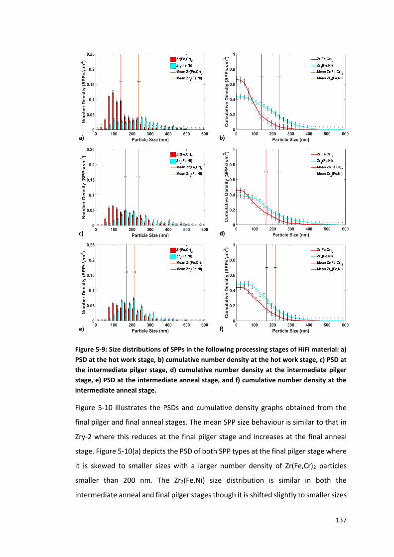
137

Figure 5-9: Size distributions of SPPs in the following processing stages of HiFi material: a)

PSD at the hot work stage, b) cumulative number density at the hot work stage, c) PSD at

the intermediate pilger stage, d) cumulative number density at the intermediate pilger

stage, e) PSD at the intermediate anneal stage, and f) cumulative number density at the

intermediate anneal stage.

Figure 5-10 illustrates the PSDs and cumulative density graphs obtained from the

final pilger and final anneal stages. The mean SPP size behaviour is similar to that in

Zry-2 where this reduces at the final pilger stage and increases at the final anneal

stage. Figure 5-10(a) depicts the PSD of both SPP types at the final pilger stage where

it is skewed to smaller sizes with a larger number density of Zr(Fe,Cr)2 particles

smaller than 200 nm. The Zr2(Fe,Ni) size distribution is similar in both the

intermediate anneal and final pilger stages though it is shifted slightly to smaller sizes

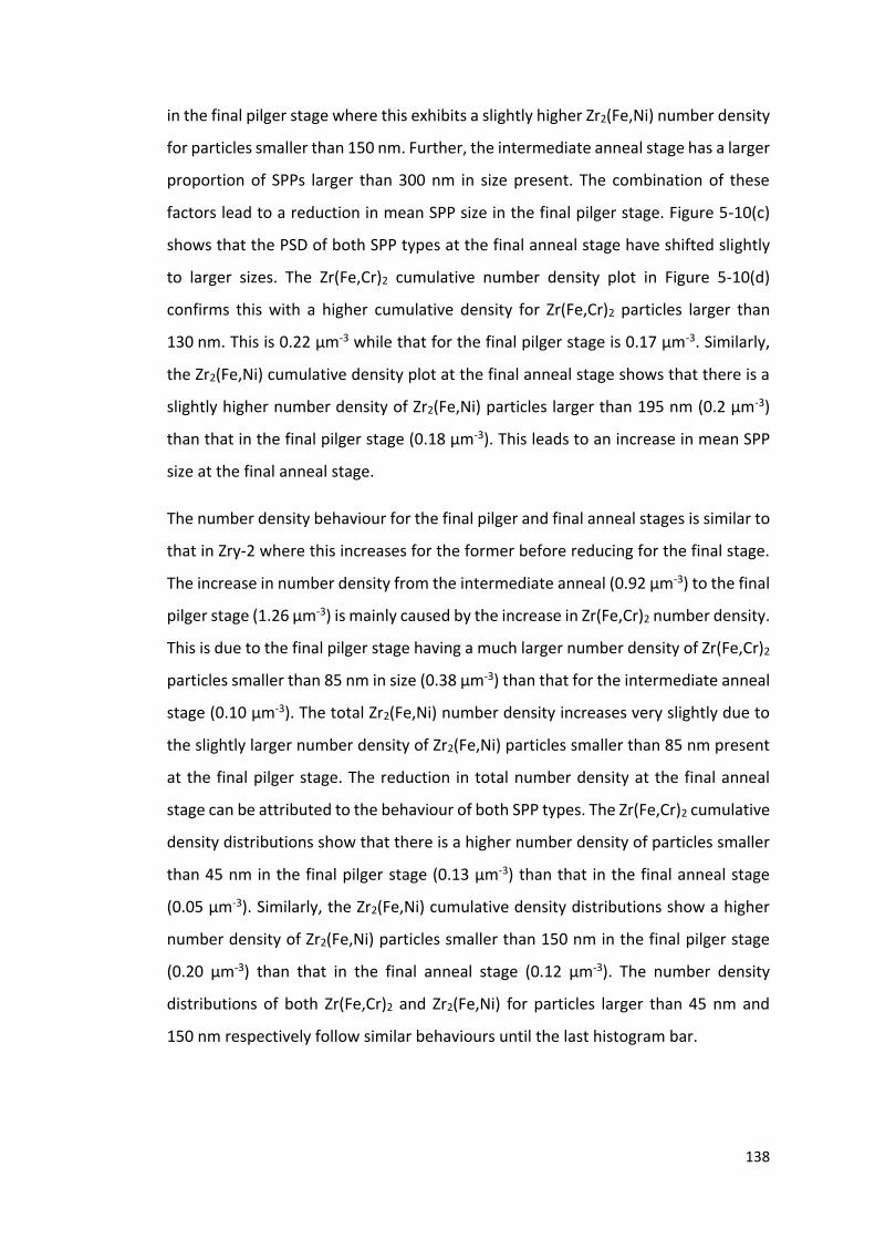
138

in the final pilger stage where this exhibits a slightly higher Zr2(Fe,Ni) number density

for particles smaller than 150 nm. Further, the intermediate anneal stage has a larger

proportion of SPPs larger than 300 nm in size present. The combination of these

factors lead to a reduction in mean SPP size in the final pilger stage. Figure 5-10(c)

shows that the PSD of both SPP types at the final anneal stage have shifted slightly

to larger sizes. The Zr(Fe,Cr)2 cumulative number density plot in Figure 5-10(d)

confirms this with a higher cumulative density for Zr(Fe,Cr)2 particles larger than

130 nm. This is 0.22 μm-3 while that for the final pilger stage is 0.17 μm-3. Similarly,

the Zr2(Fe,Ni) cumulative density plot at the final anneal stage shows that there is a

slightly higher number density of Zr2(Fe,Ni) particles larger than 195 nm (0.2 μm-3)

than that in the final pilger stage (0.18 μm-3). This leads to an increase in mean SPP

size at the final anneal stage.

The number density behaviour for the final pilger and final anneal stages is similar to

that in Zry-2 where this increases for the former before reducing for the final stage.

The increase in number density from the intermediate anneal (0.92 μm-3) to the final

pilger stage (1.26 μm-3) is mainly caused by the increase in Zr(Fe,Cr)2 number density.

This is due to the final pilger stage having a much larger number density of Zr(Fe,Cr)2

particles smaller than 85 nm in size (0.38 μm-3) than that for the intermediate anneal

stage (0.10 μm-3). The total Zr2(Fe,Ni) number density increases very slightly due to

the slightly larger number density of Zr2(Fe,Ni) particles smaller than 85 nm present

at the final pilger stage. The reduction in total number density at the final anneal

stage can be attributed to the behaviour of both SPP types. The Zr(Fe,Cr)2 cumulative

density distributions show that there is a higher number density of particles smaller

than 45 nm in the final pilger stage (0.13 μm-3) than that in the final anneal stage

(0.05 μm-3). Similarly, the Zr2(Fe,Ni) cumulative density distributions show a higher

number density of Zr2(Fe,Ni) particles smaller than 150 nm in the final pilger stage

(0.20 μm-3) than that in the final anneal stage (0.12 μm-3). The number density

distributions of both Zr(Fe,Cr)2 and Zr2(Fe,Ni) for particles larger than 45 nm and

150 nm respectively follow similar behaviours until the last histogram bar.

139

Figure 5-10: Size distributions of SPPs in the following processing stages of HiFi material: a)

PSD at the final pilger stage, b) cumulative number density at the final pilger stage, c) PSD

at the final anneal stage, d) cumulative number density at the final anneal stage.

5.4 Effect of Thermomechanical Processes on SPP

Characteristics

5.4.1 Effect of Hot Extrusion

The SPP distribution formed from the β-quench stage is subject to change from prior

extrusion heat treatment, the hot work process, and the subsequent air cooling.

Figure 5-11 illustrates the potential mechanism for the SPP evolution.

140

Figure 5-11: Schematic showing the potential mechanism for SPP evolution throughout the

hot extrusion process where the red particles represent Zr(Fe,Cr)2, the blue particles

represent Zr2(Fe,Ni) , and the black lines represent grain boundaries. Grain growth takes

place throughout the extrusion process. SPPs grow and coalesce during the prior extrusion

heat treatment. During hot extrusion, smaller SPPs dissolve and solutes distribute

throughout the matrix, leading the SPP growth/coarsening and nucleation of small SPPs.

Grain distortion is also present the extrusion process. Subsequent air cooling lead to

further grain growth and SPP coarsening.

After the β-quench stage, the material is subject to a heat treatment from room

temperature to a high temperature α-Zr phase region. As shown in Figure 5-11, the

α-Zr lamellae structure is replaced by large grains and the small SPPs are thought to

coalesce and grow slightly. At the high temperature, the solubility limit is higher and

therefore there should be a lower volume fraction of SPPs present in the system (if

equilibrium is reached). However, the volume fraction of SPPs obtained after the hot

work process is larger than that obtained after the β-quench stage in Zry-2 where the

total SPP volume fraction increases from 0.0040 to 0.0086. The total SPP volume

fraction in HiFi increases from 0.0093 to 0.0155 from the β-quench stage to the hot

work stage. In addition, as seen in Figure 5-5 (a) and Figure 5-8(a), the SPP volume

fraction for Zry-2 and HiFi at the hot extrusion process is larger than that identified

at the lower temperature anneals performed at the intermediate and final anneal

stages. This suggests that SPP coarsening takes place during the subsequent

extrusion and slow cooling.

141

The high SPP volume fraction could result from the extrusion process though this

cannot be confirmed. However, the high deformation in this process does lead to a

more homogeneous distribution of SPPs (Figure 5-12) with the exception of SPPs that

are attached to one another. This is consistent with the study performed with

Liu et al. on hot rolled Zr-Sn-Nb-Fe-Cr alloy where SPPs were homogenously

distributed in α-Zr grains [106]. However, the hot rolling operation was performed at

60 % reduction, which is lower than that used in the hot extrusion of the β-quenched

material in this study. As shown by Chen et al. [68], a larger reduction leads to a

distorted microstructure though this was performed at temperatures less than

600 °C. At higher temperatures, this distortion is thought to be present, due to the

combination of recovery and recrystallization, though to a lesser extent [168]. In

addition, the material increases in temperature during the hot extrusion process

from that obtained during the prior extrusion heat treatment to that very close to

the (α-Zr + β-Zr) phase region [69]. From Section 4.2, the SPPs dissolve into the matrix

at temperatures close to the α-Zr to β-Zr phase transformation temperature so there

could be a redistribution of solutes during the deformation process. This has the

potential to either accelerate the particle coarsening process or redistribute solutes

such that new precipitates form on cooling after the extrusion process due to the

increase in supersaturation.

Figure 5-12: ESB images taken on the SEM of SPPs at the hot work stage in: a) Zry-2, and b)

HiFi.

Subsequent air cooling is thought to be approximately 4 °C/s from the high

temperature to room temperature [37]. Since SPPs have already been formed during

the β-quench and hot extrusion processes, it is thought that SPP coarsening regime

142

is dominant. With a slow cooling rate, large SPPs and a high SPP volume fraction are

present. This is attributed to the fact that with the slower cooling rate, the

equilibrium concentration of solutes in the matrix is approached [37], resulting in an

excess of SPPs present in the system. From the PSDs for both Zry-2 and HiFi,

illustrated in Figure 5-6(a) and Figure 5-9(a) respectively, SPPs as large as 500 nm

have been identified. This suggests that the SPP growth regime, if present, has taken

place during the prior extrusion heat treatment. However, SPP coarsening is most

likely prominent throughout the hot work process since the PSDs are broader and at

larger SPP sizes than those obtained after β-quenching (Figure 5-4).

5.4.2 Effect of Cold Work

The cold pilger process reduces the mean SPP size in both alloys by a maximum of

30 nm. This differs from a study by Garzarolli et al. that examined the effect of 𝛸CAP

on mean SPP size where it was hypothesised that cold work has no effect on SPP

size [44]. On the other hand, the decrease in SPP size due to cold work has been

experimentally shown by Qiu et al. where the authors performed a maximum cold

reduction of 50 % on Zr-1.0Sn-1.0Nb-0.12Fe alloy [70]. However, in this study the

minimum reduction performed on the tube material is 75 %. In addition to this, cold

pilgering performed on Zry-2 and HiFi generally increases the SPP number density by

a maximum of 0.2 µm-3. The exception to this is at the intermediate pilger stage for

HiFi. Nevertheless, this increase in SPP number density with the reduced mean SPP

size can result from either the nucleation of new small particles which would require

a very strong accelerating effect of the deformation induced defects (vacancies and

dislocations), or SPPs being broken or sheared into smaller pieces.

Cold pilgering induces a high dislocation density in the material and excess vacancies.

Both of these factors can greatly accelerate diffusion, clustering, and nucleation of

new small SPPs. However, even with this strong acceleration, diffusion distances at

room temperature (cold deformation) of the relevant solutes in Zr, are expected to

be too low for new precipitation to form under cold conditions. Therefore, solute

diffusion and formation of new clusters is not thought to be a potential mechanism

for the change in SPP distribution.

143

The reduction in SPP size and increase in number density could be attributed to the

crushing or shearing of large SPPs. The SPPs that have been subject to shearing would

then lead to a cluster of SPPs in that location. An example of this is displayed in

Figure 5-13 where two clusters of Zr2(Fe,Ni) particles are highlighted. These have an

effective size range of 80-216 nm in the image and it can be assumed that these could

have originated from larger Zr2(Fe,Ni) particles since they are in close proximity. With

these SPP clusters, the Zr2(Fe,Ni) particle number density in this image is 0.62 µm-3

while this reduces to 0.37 µm-3 if there were only two large Zr2(Fe,Ni) particles

instead of the clusters. The Zr2(Fe,Ni) mean size in turn increases from 131.4 nm to

169.5 nm assuming that the two larger Zr2(Fe,Ni) particles are present instead of the

smaller ones. This concept of particle shearing does not seem to take place

frequently. Table 5-2 illustrates this where the largest SPP size for both SPP types

does not always reduce when pilgering takes place. In addition to this, the SPPs

appear to be undeformed after the pilger process. Nonetheless, if particle shearing

takes place on a sufficient number of SPPs, the overall number density and mean size

would be affected such that it can be observed in Figure 5-5 and Figure 5-8.

Figure 5-13: SPP clustering at the intermediate pilger stage in Zry-2.

144

Table 5-2: Largest Zr(Fe,Cr)2 and Zr2(Fe,Ni) size in Zry-2 and HiFi at each processing stage.

Zry-2 HiFi

Zr(Fe,Cr)2 Zr2(Fe,Ni) Zr(Fe,Cr)2 Zr2(Fe,Ni)

Hot Extrusion 277 nm 382 nm 483 nm 491 nm

Inter. Pilger 315 nm 336 nm 491 nm 461 nm

Inter. Anneal 284 nm 508 nm 377 nm 573 nm

Final Pilger 257 nm 362 nm 377 nm 474 nm

Final Anneal 287 nm 343 nm 458 nm 460 nm

5.4.3 Effect of Annealing

Each annealing step was performed at an intermediate temperature in the α-Zr phase

region and held at this temperature for the same period of time at each annealing

stage. Annealing after pilgering leads to a maximum increase in SPP size of 21 nm in

both alloys. The maximum reduction in SPP number density from pilger to anneal

stage in both alloys is 0.13 µm-3. The exception to these observations in mean size

and number density is seen at the intermediate anneal stage for HiFi (Section 5.3.2).

Nonetheless, the increase in SPP size is similar to that shown by Qiu et al. on Zr-1.0Sn-

1.0Nb-0.12Fe alloy, cold worked with a reduction of 50 % and subsequently annealed

at 590 °C for 2 hr [70]. It should be noted though this heat treatment is slightly higher

in temperature than the heat treatments used in the processing route in the present

study, although the annealing time is similar. The higher imposed deformation

(percentage reduction) in addition to the different heat treatment used in this study

leads to a smaller increase in average SPP size than that shown by Qiu et al. with an

increase in mean SPP size of 10 nm.

The effect of processing on mean SPP size in Zry-2 cladding material has also been

examined by Garzarolli et al. [44]. This is shown as a relationship between 𝛸CAP and

the mean SPP size where both Zr2(Fe,Ni) and Zr(Fe,Cr)2 particles are considered

(Figure 5-14). In addition, the mean SPP size obtained after final annealing for Zry-2

in this study is displayed in Figure 5-14. The 𝛸CAP value for the processing route used

in this study was 3.89 × 10−18 hr. This assumes that the heat treatment prior to

extrusion was performed at a constant temperature though, in reality, the

temperature profile is relatively linear from room temperature to the target

temperature. The dashed red line in Figure 5-14 is an interpolation between the data

points at 2.51 × 10−18 hr and 1.72 × 10−17 hr. At 3.89 × 10−18 hr, the interpolation

145

from Garzarolli et al. suggests that the mean SPP size should be 91 nm. However, the

mean SPP size in Zry-2 from this study is 80 nm. The difference in mean SPP size is

thought to result from the fact that the Zry-2 samples in the study performed by

Garzarolli et al. were taken from different processing routes. These samples would

have undergone differing heat treatments and thus these may cancel out potential

effects that cold work has on SPP size distributions.

Figure 5-14: The effect of CAP on mean SPP size in Zry-2 production cladding material,

adapted from [44].

Figure 5-5(a) and Figure 5-8(a) show that from the intermediate pilger stage to the

final anneal stage in both alloys, the SPP volume fraction decreases slightly. This

suggests that the equilibrium volume fraction of SPPs at the intermediate/final

anneal temperature is still exceeded even though a large reduction in SPP volume

fraction is observed at the intermediate pilger stage. Despite this, the particle

coarsening regime seems to be present in the anneal stages since the mean SPP size

is increasing while the particle number density generally decreases for both SPP

types.

The increase in mean size from pilger to anneal stages could also be attributed to

solute diffusion from particle to particle. Figure 5-15 illustrates a schematic of the

mechanism for SPP coarsening. Initially, solutes are present in SPPs assuming that

the matrix is fully depleted of solute. During annealing, solutes diffuse from smaller

to larger particles since the equilibrium solute concentration at the particle/matrix

interface is higher for the smaller particles than that for the larger particles. As a

146

result, a concentration gradient is present between the smaller and larger particles.

Particle coarsening can be accelerated by the presence of dislocations though this is

not critical to the process.

Figure 5-15: Schematic showing the effect of annealing on solute diffusion where 𝐜𝛉 is the

solute concentration, 𝛗 resembles a SPP, 𝐜𝛉𝛂𝛗

is the solute concentration at the

particle/matrix interface, 𝐯𝟏 and 𝐯𝟐 are the velocities of SPP growth/dissolution of the two

SPPs, and 𝐉𝛉 is the solute concentration gradient between the small and large SPPs.

Adapted from [123].

The increase in mean SPP size observed in Figure 5-5(b) and Figure 5-8(b) could also

be attributed to the amalgamation of multiple particles into one larger particle.

Figure 5-16 shows an example of this where two initially separated Zr2(Fe,Ni)

particles are merged into one as a result of the diffusion of Fe or Ni. The new particle

is then considered as one large particle with a larger mean size. For example, the

large Zr2(Fe,Ni) particle in Figure 5-16 has an effective particle size of 194 nm while

before the amalgamation the two smaller Zr2(Fe,Ni) particles would have an effective

particle size of 125 nm and 145 nm.

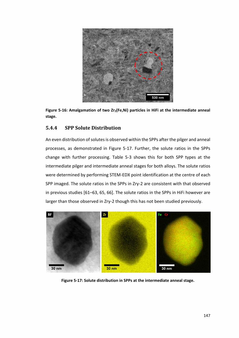
147

Figure 5-16: Amalgamation of two Zr2(Fe,Ni) particles in HiFi at the intermediate anneal

stage.

5.4.4 SPP Solute Distribution

An even distribution of solutes is observed within the SPPs after the pilger and anneal

processes, as demonstrated in Figure 5-17. Further, the solute ratios in the SPPs

change with further processing. Table 5-3 shows this for both SPP types at the

intermediate pilger and intermediate anneal stages for both alloys. The solute ratios

were determined by performing STEM-EDX point identification at the centre of each

SPP imaged. The solute ratios in the SPPs in Zry-2 are consistent with that observed

in previous studies [61–63, 65, 66]. The solute ratios in the SPPs in HiFi however are

larger than those observed in Zry-2 though this has not been studied previously.

Figure 5-17: Solute distribution in SPPs at the intermediate anneal stage.

148

Table 5-3: Fe/Ni and Fe/Cr solute ratios respectively in Zr2(Fe,Ni) and Zr(Fe,Cr)2 in Zry-2 and

HiFi at the intermediate pilger stage, the intermediate anneal stage, and under equilibrium

conditions at the intermediate temperature as predicted by JMatPro [188].

Zry-2 HiFi

Fe/Ni Fe/Cr Fe/Ni Fe/Cr

Intermediate Pilger

1.58 ± 0.02 0.77 ± 0.02 3.68 ± 0.06 1.53 ± 0.05

Intermediate Anneal

1.50 ± 0.01 0.76 ± 0.02 3.53 ± 0.03 1.44 ± 0.04

Equilibrium Solute Ratio

3.03 0.65 7.42 0.79

The solute ratios in the SPPs in both Zry-2 and HiFi at the intermediate pilger stage

seem to vary with SPP size. However, as illustrated in Figure 5-18, the variation in

solute concentration with SPP size appears to be small. Nonetheless, this slight

variation in solute ratio with SPP size present in both alloys prior to the annealing

suggests particle coarsening has taken place in the previous thermomechanical

processing stages. Figure 5-18(a) shows that the Fe/Ni ratio reduces slightly with

increasing Zr2(Fe,Ni) particle size. This suggests that as the Zr2(Fe,Ni) particle grows

in size, they enrich in Ni. However, clearly this is only the case if the Zr2(Fe,Ni)

particles are present in the system to begin with. The same can be interpreted with

the reduction in Fe/Cr ratio with increasing Zr(Fe,Cr)2 size in HiFi at the intermediate

pilger stage, as shown in Figure 5-18(b). At the same time, Figure 5-18(a) also shows

that the Fe/Cr ratio in Zr(Fe,Cr)2 particles in Zry-2 slightly increases with SPP size and

Figure 5-18(b) demonstrates that the Fe/Ni solute ratio in HiFi also increases slightly

with SPP size. The difference in solute ratio with SPP size is attributed with the

competition between the different SPP types for the available Fe and the relative

volume fraction of each phase. Nevertheless, after the intermediate pilger stage, the

changes in solute ratio with SPP size in SPPs in both Zry-2 and HiFi are very small and

are not likely to be significant.

149

Figure 5-18: Variation in solute ratio (obtained using STEM-EDX) with SPP size at the

intermediate pilger stage where: a) shows Fe/Ni and Fe/Cr ratios in Zry-2, and b) shows

Fe/Ni and Fe/Cr ratios in HiFi in Zr2(Fe,Ni) and Zr(Fe,Cr)2 respectively.

From Table 5-3, the average SPP solute ratio reduces from the intermediate pilger

stage to the intermediate annealing stage though this is marginal. Figure 5-19 depicts

this for both SPP types in both alloys. Figure 5-19(a) show that in Zry-2, the annealing

process leads to a slight reduction in Fe/Ni solute ratio in the observed SPP sizes. This

suggests that SPP coarsening is taking place since the SPPs after the intermediate

anneal stage is richer in the slower diffuser i.e. Ni. The Fe/Cr ratio in Zry-2 after

annealing exhibits a similar trend though this reduction in solute ratio is smaller,

maybe within error. This observation is consistent with observations by Yang et al.

on the Fe/Cr and Fe/Ni solute ratio changes on Zry-2 heat treated at 576 °C [62]. The

solute ratios in HiFi after annealing, illustrated in Figure 5-19(b), do not show a net

increase or reduction after annealing.

Figure 5-19: Variation in solute ratio (obtained using STEM-EDX) with SPP size where: a)

shows Fe/Ni and Fe/Cr ratios in Zry-2 at the intermediate pilger and intermediate anneal

stages, b) shows Fe/Ni and Fe/Cr ratios in HiFi at the intermediate pilger and intermediate

anneal stages.

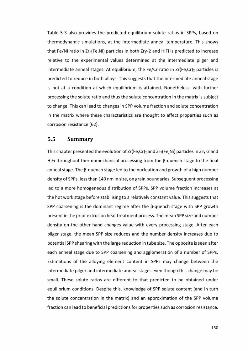
150

Table 5-3 also provides the predicted equilibrium solute ratios in SPPs, based on

thermodynamic simulations, at the intermediate anneal temperature. This shows

that Fe/Ni ratio in Zr2(Fe,Ni) particles in both Zry-2 and HiFi is predicted to increase

relative to the experimental values determined at the intermediate pilger and

intermediate anneal stages. At equilibrium, the Fe/Cr ratio in Zr(Fe,Cr)2 particles is

predicted to reduce in both alloys. This suggests that the intermediate anneal stage

is not at a condition at which equilibrium is attained. Nonetheless, with further

processing the solute ratio and thus the solute concentration in the matrix is subject

to change. This can lead to changes in SPP volume fraction and solute concentration

in the matrix where these characteristics are thought to affect properties such as

corrosion resistance [62].

5.5 Summary

This chapter presented the evolution of Zr(Fe,Cr)2 and Zr2(Fe,Ni) particles in Zry-2 and

HiFi throughout thermomechanical processing from the β-quench stage to the final

anneal stage. The β-quench stage led to the nucleation and growth of a high number

density of SPPs, less than 140 nm in size, on grain boundaries. Subsequent processing

led to a more homogeneous distribution of SPPs. SPP volume fraction increases at

the hot work stage before stabilising to a relatively constant value. This suggests that

SPP coarsening is the dominant regime after the β-quench stage with SPP growth

present in the prior extrusion heat treatment process. The mean SPP size and number

density on the other hand changes value with every processing stage. After each

pilger stage, the mean SPP size reduces and the number density increases due to

potential SPP shearing with the large reduction in tube size. The opposite is seen after

each anneal stage due to SPP coarsening and agglomeration of a number of SPPs.

Estimations of the alloying element content in SPPs may change between the

intermediate pilger and intermediate anneal stages even though this change may be

small. These solute ratios are different to that predicted to be obtained under

equilibrium conditions. Despite this, knowledge of SPP solute content (and in turn

the solute concentration in the matrix) and an approximation of the SPP volume

fraction can lead to beneficial predictions for properties such as corrosion resistance.

151

6 Simulating Precipitation Kinetics in Zircaloy-2

and HiFi

SPP precipitation kinetics in Zry-2 and HiFi is simulated using a modified version of

the KWN model. The operation of the basic KWN model is discussed before

introducing features added to the framework. Input parameters are also presented.

Model calibration is performed using experimental data shown in Chapter 4.

Subsequently, the KWN model is applied to simulate the annealing processes present

in thermomechanical processing. The resulting simulation is compared to

experimental data-sets.

6.1 KWN Model Operation

Figure 6-1 illustrates the operation of the basic KWN framework for the precipitation

kinetics of spherical particles.

Figure 6-1: Operation of the KWN model, adapted from [133].

The total simulation time is divided into smaller time steps where both the PSD and

matrix solute concentration are discretised. Within each time step, the critical

particle radius is calculated (Equation 2-7) and, in conjunction with critical free

energy (Equation 2-8) and nucleation rate (Equation 2-9) expressions, the number of

new particles can be determined [130]. To prevent the immediate dissolution of new

152

particles, the radius of newly formed particles are arbitrarily set to be 10 % larger

than the critical radius. These particles are then allocated to the correct PSD size

class [130, 133]. Thereafter, the growth rate of all particles is calculated by using

Equation 2-14 on the upper and lower edges of each size class. This computation then

allows the reallocation of the particles from each size class. Figure 6-2 illustrates an

example of this where particles originally from the size class 2 are distributed over

classes 3-5 when growth rates 𝑣L and 𝑣U are applied to the lower (L) and upper (U)

size class edges at time 𝑡 and 𝑡 + ∆𝑡 respectively [131]. Here, the assumption made

is that diffusion controlled growth occurs. Additionally, the Gibbs-Thomson effect is

considered when calculating the new compositions at the interface of each particle

in each size class. Subsequently, the new PSD and precipitate volume fraction are

determined. As a result, the matrix solute concentration is computed using the mean

field approximation [130–134, 150]. These characteristics are then used in the

subsequent time step.

Figure 6-2: Reallocation of particles from size class 2 to classes 3-5 after the application of

growth rates 𝒗𝐋 and 𝒗𝐔 where 𝐋 and 𝐔 are the lower and upper edges of the size class,

adapted from [131].

Model efficiency and accuracy are attained by employing an adaptive time step

within a Runge-Kutta scheme. This updates the PSD at each iteration. The time

interval is adjusted to ensure that errors in particle number density and particle

radius are less than 0.001 particles/µm3 and 0.001 nm respectively between each

step. This is most prominent in early stages of precipitation kinetics. Here, rapid

nucleation and growth rates of particles are observed and thus the time step is

minimised to ensure that the aforementioned error criteria are met. In later

precipitation stages, the time step increases as fewer changes in kinetics are

observed [131].

153

6.2 Additional Features

The KWN model used in this study is based on that used by Robson though irradiation

effects on SPPs are not considered here [150]. Improved accuracy of the model is

achieved by considering the following features:

6.2.1 Precipitation of Multiple SPPs

Both Zry-2 and HiFi have Zr(Fe,Cr)2 and Zr2(Fe,Ni) particles. For simplicity, binary

systems are used to describe both SPP types with the main alloying elements

considered as the effective solute, similar to that used by Robson [150], and Massih

and Jernkvist [151]. The Zr(Fe,Cr)2 particle is considered as a Zr-(Fe+Cr) system and

the Zr2(Fe,Ni) particle is considered as a Zr-(Fe+Ni) system.

In the original model, only a single precipitate type was considered and thus the true

precipitation behaviour when two precipitate phases are involved in not captured.

Instead, the binary systems can be separated to form independent models with Fe

shared between the two SPP types. Additionally, the proportion of Fe to either Cr or

Ni changes with an additional heat treatment (Section 5.4.4) though this appears to

be minimal. The different SPP types thus affect the solute concentration present in

both SPP systems. The Zr-(Fe+Cr) and Zr-(Fe+Ni) systems can be coupled, as

demonstrated by Ouden et al. [152] however, the exact quantity of Fe present in SPPs

is unknown since the SPP composition has been established in terms of solute ratios.

Therefore, the SPP systems are left uncoupled for simplicity.

6.2.2 Heterogeneous Nucleation of SPPs

Chapter 5 shows that SPPs in both Zry-2 and HiFi can nucleate on grain boundaries.

The proportion of SPPs forming on grain boundaries relative to SPP formation in the

grain interior by number is higher when deformation is not present. An example of

this is shown in Table 6-1 where SPPs were analysed in Zry-2 and HiFi samples that

were β-quenched at a cooling rate of approximately 1500 °C/s, followed by

isothermal anneals at 600 °C and 700 °C.

154

Table 6-1: Proportion of SPPs, by number, formed in the grain interior and on grain

boundaries in Zry-2 and HiFi, isothermally heat treated at 600 °C or 700 °C.

Zry-2 HiFi

600 °C / 20 hr 700 °C / 2 hr 600 °C / 10 hr 700 °C / 1 hr

Grain 17.5 % 7.0 % 13.3 % 20.7%

Grain Boundary 82.5 % 93.0 % 86.7 % 79.3 %

It can be seen that regardless of state, grain boundary precipitation is the dominant

mode and it is the larger grain boundary precipitates, captured in the SEM images,

which are used to calibrate the model. Therefore, the model is applied to, and fitted

to, grain boundary precipitation. It could also be used for grain interior precipitation

though this would require a different set of calibration parameters.

Grain boundary precipitation results in a reduction in the effective interfacial energy.

This takes place when the precipitation of the SPP leads to the destruction of the

grain boundary that lies within the SPP [121]. Equation 2-13 expresses this. The

reduction in the effective interfacial energy is accounted for in the model through

the calibration process, which is used to fix this parameter to provide good

agreement between the predicted and measured precipitation kinetics.

6.2.3 Co-Precipitation

SPPs in Zry-2 and HiFi can precipitate from one another heterogeneously, as

demonstrated in Section 4.1.2. However, the proportion of SPPs co-precipitating

from one another is small by number in comparison to SPPs nucleating

independently. Table 6-2 summarises this quantitatively for Zry-2 and HiFi

isothermally annealed at 600 °C or 700 °C from the β-quenched condition. The

mechanism of the co-precipitation effect is not yet understood, and the relatively

small contribution these particles make to the overall PSD means that the co-

precipitation mechanism was not explicitly captured in the present simulation. Once

the mechanism of co-precipitation is better understood, this mechanism could also

be explicitly be included within the modelling framework presented here.

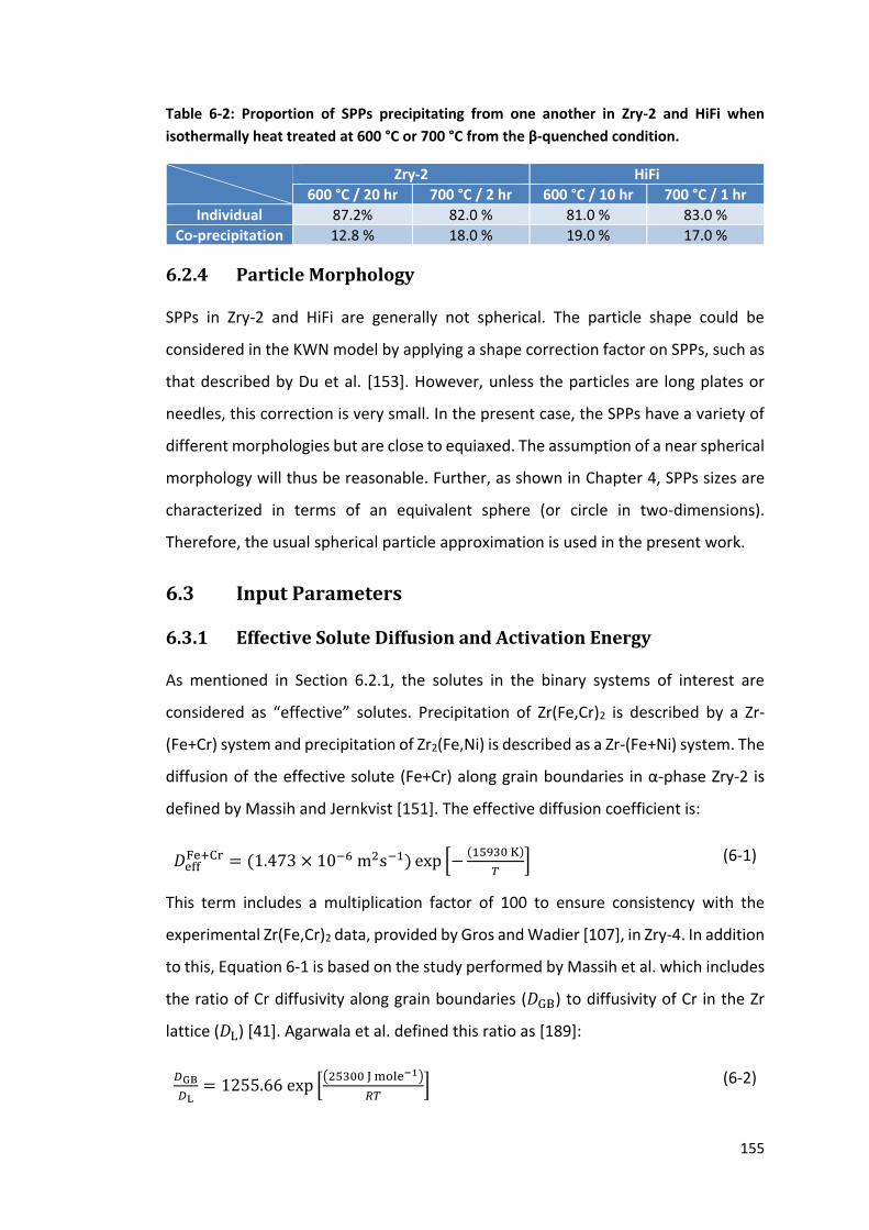
155

Table 6-2: Proportion of SPPs precipitating from one another in Zry-2 and HiFi when

isothermally heat treated at 600 °C or 700 °C from the β-quenched condition.

Zry-2 HiFi

600 °C / 20 hr 700 °C / 2 hr 600 °C / 10 hr 700 °C / 1 hr

Individual 87.2% 82.0 % 81.0 % 83.0 %

Co-precipitation 12.8 % 18.0 % 19.0 % 17.0 %

6.2.4 Particle Morphology

SPPs in Zry-2 and HiFi are generally not spherical. The particle shape could be

considered in the KWN model by applying a shape correction factor on SPPs, such as

that described by Du et al. [153]. However, unless the particles are long plates or

needles, this correction is very small. In the present case, the SPPs have a variety of

different morphologies but are close to equiaxed. The assumption of a near spherical

morphology will thus be reasonable. Further, as shown in Chapter 4, SPPs sizes are

characterized in terms of an equivalent sphere (or circle in two-dimensions).

Therefore, the usual spherical particle approximation is used in the present work.

6.3 Input Parameters

6.3.1 Effective Solute Diffusion and Activation Energy

As mentioned in Section 6.2.1, the solutes in the binary systems of interest are

considered as “effective” solutes. Precipitation of Zr(Fe,Cr)2 is described by a Zr-

(Fe+Cr) system and precipitation of Zr2(Fe,Ni) is described as a Zr-(Fe+Ni) system. The

diffusion of the effective solute (Fe+Cr) along grain boundaries in α-phase Zry-2 is

defined by Massih and Jernkvist [151]. The effective diffusion coefficient is:

𝐷effFe+Cr = (1.473 × 10−6 m2s−1) exp [−

(15930 K)

𝑇] (6-1)

This term includes a multiplication factor of 100 to ensure consistency with the

experimental Zr(Fe,Cr)2 data, provided by Gros and Wadier [107], in Zry-4. In addition

to this, Equation 6-1 is based on the study performed by Massih et al. which includes

the ratio of Cr diffusivity along grain boundaries (𝐷GB) to diffusivity of Cr in the Zr

lattice (𝐷L) [41]. Agarwala et al. defined this ratio as [189]:

𝐷GB

𝐷L= 1255.66 exp [

(25300 J mole−1)

𝑅𝑇] (6-2)

156

Since grain boundary precipitation is only considered in this study, Equation 6-1 is

used as the effective diffusivity of (Fe+Cr). However, the original model used by

Massih et al. [41] was tested against a distribution of SPPs measured in Zry-2 where

both SPP types are considered. Further, Massih and Jernkvist [151] attempted to

maintain consistency with the data from Gros and Wadier which considered SPPs in

Zry-4 [107]. In general, Zry-4 has a larger volume fraction of Zr(Fe,Cr)2 than in Zry-2.

Therefore, a pre-exponential factor – a reduction in effective diffusivity by a factor of

750 – has been introduced to take into account the smaller Zr(Fe,Cr)2 volume fraction

in Zry-2 than that in the aforementioned studies. Equation 6-3 demonstrates the

modified effective diffusivity of (Fe+Cr) in Zry-2:

𝐷effFe+Cr = (

1.473×10−6

750m2s−1) exp [−

(15930 K)

𝑇] (6-3)

The diffusivity of (Fe+Ni), 𝐷effFe+Ni, has not been defined in literature. However, the

diffusion of Fe, Cr, and Ni in α-phase Zry-2 was reported by Pande et al. [190], and

Pande and Agarwala [191] in the temperature range of 650-780 °C. Equation 6-4,

Equation 6-5 and Equation 6-6 depict this (where 𝑅 is the universal gas constant and

𝑇 is the temperature in kelvin), and Figure 6-3 illustrates the change in diffusivity of

Fe, Cr, and Ni in Zry-2 with temperature.

𝐷Feα Zry−2

= (2.56 × 10−12 m2s−1) exp [−(112700 J mole−1)

𝑅𝑇] (6-4)

𝐷Crα Zry−2

= (2.91 × 10−10 m2s−1) exp [−(148900 J mole−1)

𝑅𝑇] (6-5)

𝐷Niα Zry−2

= (1.00 × 10−11 m2s−1) exp [−(122400 J mole−1)

𝑅𝑇] (6-6)

157

Figure 6-3: Lattice diffusivity of Fe, Cr, and Ni in α-Zr in Zry-2 with temperature.

The diffusivities of Fe and Ni are very similar and therefore 𝐷effFe+Ni can be estimated

by using 𝐷Niα Zry−2

. This term can be determined by first considering the difference

between 𝐷Crα Zry−2

from Pande et al. [190] and 𝐷effFe+Cr defined by Massih and

Jernkvist. These terms were compared against temperature (Figure 6-4) though the

diffusivity term by Massih and Jernkvist does not include Equation 6-2. The two plots

are nearly identical except at low temperatures where a small deviation is present.

Therefore, Equation 6-1 can be redefined as a multiplication of Equation 6-5 and

Equation 6-3. Figure 6-3 also shows that 𝐷Crα Zry−2

and 𝐷Niα Zry−2

are within less than a

factor of 10 at annealing temperatures above 500 °C (used for industrial heat

treatments). As a result, it can be assumed that 𝐷Crα Zry−2

and 𝐷Niα Zry−2

are similar and

thus 𝐷effFe+Ni can be defined with the grain boundary to lattice diffusivity ratio defined

in Equation 6-2. Including the aforementioned factor, 𝐷effFe+Ni is defined as:

𝐷effFe+Ni =

1

750

𝐷GB

𝐷L𝐷Ni

α Zry−2 (6-7)

158

Figure 6-4: Diffusivity vs. temperature of 𝑫𝐂𝐫𝛂 𝐙𝐫𝐲−𝟐

from Pande et al. [190], and 𝑫𝐞𝐟𝐟𝐅𝐞+𝐂𝐫 from

Massih and Jernkvist [151] without the diffusivity ratio for Cr along grain boundaries

relative to that within grains in α-Zr.

It should be noted that the effective diffusivities of (Fe+Cr) and (Fe+Ni) are

dependent on the individual diffusivity of Fe, Cr, and Ni. From Figure 6-3, the diffusion

of Cr and Ni in α-Zr grains are the rate limiting factors since they are slower diffusers

than Fe. Therefore, if the exact chemistry of the SPPs in Zry-2 and HiFi (at different

processing steps) are known, Equation 6-3 and Equation 6-7 will be subject to change

to reflect this.

6.3.2 SPP Molar Volume

The molar volume is the volume of one mole of atoms in the product phase. This is

defined in Equation 6-8.

𝑉m = 𝑀

𝜌 (6-8)

where 𝑉𝑚 is the molar volume , 𝑀 is the molar mass, and 𝜌 is the precipitate density.

The molar volume of Zr(Fe,Cr)2 is taken from literature where the value has been

calculated to be 9 × 10−6 m3/mol [107, 150, 151]. On the other hand, the molar

volume of Zr2(Fe,Ni) has not been determined in literature and had to be calculated.

Using Equation 6-8, this was found to be 1.12 × 10−5 m3/mol.

159

6.3.3 Particle Interfacial Energy

The interfacial energy of a particle is the excess free energy required to form a unit

area of an interface [121]. This is likely to change with time as precipitation regimes

change from nucleation to growth and finally coarsening [123]. However, since the

KWN method attempts to capture all of these processes naturally and allows them

to occur concomitantly, it is usually assumed there is a single “effective” interfacial

energy. This value is essentially a calibration parameter that will depend on the

nucleating phase and nucleation site and influences the temperature sensitivity of

the nucleation rate. It is assumed to be temperature independent so that, once

calibrated, the same value can be used for a range of prediction temperatures. Since

the interfacial energy is very difficult to measure directly, it is assumed to be a

constant value and is found by fitting model predictions to experimental data,

checking that the derived value is within a physically sensible range.

The particle interfacial energy is also different for different particle types. The

interfacial energy for the incoherent precipitation of Zr(Fe,Cr)2 in Zry-4 has previously

been calculated to be in the range of 0.5-1.0 J/m2 [41, 107]. The incoherent

precipitation of Zr(Fe,Cr)2 in Zry-2 was found to be 0.25 J/m2 by Massih and Jernkvist

through fitting of their model [151]. Therefore, the interfacial energy for Zr(Fe,Cr)2 in

Zry-2 and HiFi is manually adjusted to quantitatively predict SPP evolution. The

interfacial energy of Zr2(Fe,Ni) has not been determined previously. It should be

noted that not all the SPPs formed in Zr alloys are fully incoherent. SPPs co-

precipitate on one another, there is an orientation relationship between the

SPPs [61], and the interface is semi-coherent [121]. However, Table 6-2 illustrates

that there are a higher proportion of lone SPPs than those that precipitate from one

another. Therefore, it is assumed that the SPPs are incoherent for the purpose of the

KWN model. In the case of grain boundary precipitation, the effective interfacial

energy also accounts for the reduction in the energy barrier to nucleation associated

with the nucleus forming on the grain boundary rather than homogeneously within

the matrix.

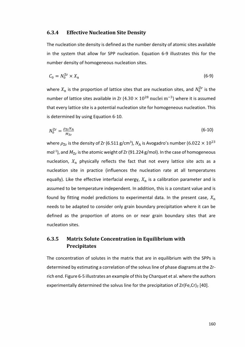
160

6.3.4 Effective Nucleation Site Density

The nucleation site density is defined as the number density of atomic sites available

in the system that allow for SPP nucleation. Equation 6-9 illustrates this for the

number density of homogeneous nucleation sites.

𝐶0 = 𝑁0Zr × 𝛸n (6-9)

where 𝛸n is the proportion of lattice sites that are nucleation sites, and 𝑁0Zr is the

number of lattice sites available in Zr (4.30 × 1028 nuclei m−3) where it is assumed

that every lattice site is a potential nucleation site for homogeneous nucleation. This

is determined by using Equation 6-10.

𝑁0Zr =

𝜌Zr𝑁A

𝑀Zr (6-10)

where 𝜌Zr is the density of Zr (6.511 g/cm3), 𝑁A is Avogadro’s number (6.022 × 1023

mol-1), and 𝑀Zr is the atomic weight of Zr (91.224 g/mol). In the case of homogeneous

nucleation, 𝛸n physically reflects the fact that not every lattice site acts as a

nucleation site in practice (influences the nucleation rate at all temperatures

equally). Like the effective interfacial energy, 𝛸n is a calibration parameter and is

assumed to be temperature independent. In addition, this is a constant value and is

found by fitting model predictions to experimental data. In the present case, 𝛸n

needs to be adapted to consider only grain boundary precipitation where it can be

defined as the proportion of atoms on or near grain boundary sites that are

nucleation sites.

6.3.5 Matrix Solute Concentration in Equilibrium with

Precipitates

The concentration of solutes in the matrix that are in equilibrium with the SPPs is

determined by estimating a correlation of the solvus line of phase diagrams at the Zr-

rich end. Figure 6-5 illustrates an example of this by Charquet et al. where the authors

experimentally determined the solvus line for the precipitation of Zr(Fe,Cr)2 [40].

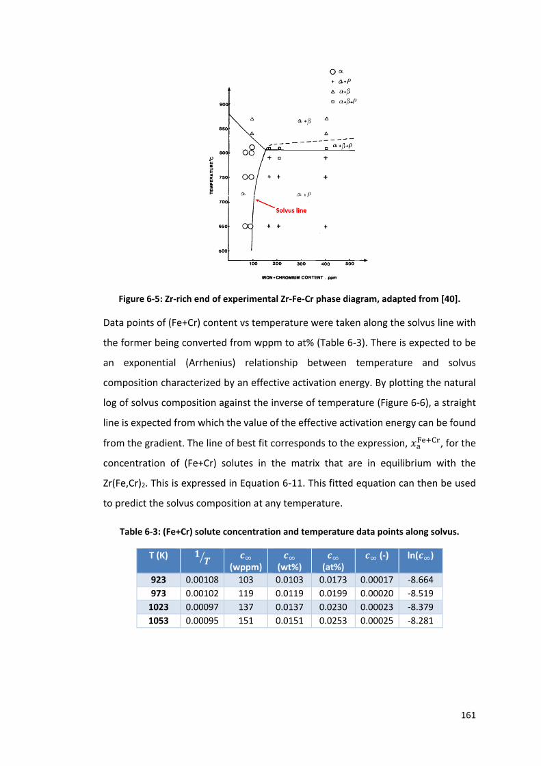
161

Figure 6-5: Zr-rich end of experimental Zr-Fe-Cr phase diagram, adapted from [40].

Data points of (Fe+Cr) content vs temperature were taken along the solvus line with

the former being converted from wppm to at% (Table 6-3). There is expected to be

an exponential (Arrhenius) relationship between temperature and solvus

composition characterized by an effective activation energy. By plotting the natural

log of solvus composition against the inverse of temperature (Figure 6-6), a straight

line is expected from which the value of the effective activation energy can be found

from the gradient. The line of best fit corresponds to the expression, 𝑥aFe+Cr, for the

concentration of (Fe+Cr) solutes in the matrix that are in equilibrium with the

Zr(Fe,Cr)2. This is expressed in Equation 6-11. This fitted equation can then be used

to predict the solvus composition at any temperature.

Table 6-3: (Fe+Cr) solute concentration and temperature data points along solvus.

T (K) 𝟏𝑻⁄ 𝒄∞

(wppm) 𝒄∞

(wt%) 𝒄∞

(at%) 𝒄∞ (-) ln(𝒄∞)

923 0.00108 103 0.0103 0.0173 0.00017 -8.664

973 0.00102 119 0.0119 0.0199 0.00020 -8.519

1023 0.00097 137 0.0137 0.0230 0.00023 -8.379

1053 0.00095 151 0.0151 0.0253 0.00025 -8.281

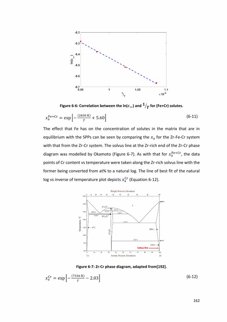
162

Figure 6-6: Correlation between the ln(𝒄∞) and 𝟏 𝑻⁄ for (Fe+Cr) solutes.

𝑥aFe+Cr = exp [−

(2830 K)

𝑇+ 5.60] (6-11)

The effect that Fe has on the concentration of solutes in the matrix that are in

equilibrium with the SPPs can be seen by comparing the 𝑥a for the Zr-Fe-Cr system

with that from the Zr-Cr system. The solvus line at the Zr-rich end of the Zr-Cr phase

diagram was modelled by Okamoto (Figure 6-7). As with that for 𝑥aFe+Cr, the data

points of Cr content vs temperature were taken along the Zr-rich solvus line with the

former being converted from at% to a natural log. The line of best fit of the natural

log vs inverse of temperature plot depicts 𝑥aCr (Equation 6-12).

Figure 6-7: Zr-Cr phase diagram, adapted from[192].

𝑥aCr = exp [−

(7336 K)

𝑇− 2.03] (6-12)

163

The concentration of solutes in the matrix in equilibrium with SPPs at the Zr-rich end

for the Zr-Cr and Zr-Fe-Cr systems are compared in Figure 6-8. The addition of the Fe

reduces solute solubility in the matrix by shifting the solvus line to smaller solute

concentrations, especially at higher temperatures. Figure 6-8 also shows the

concentration of solutes in the matrix in equilibrium with SPPs predicted by JMatPro

for the Zr-Cr and Zr-Fe-Cr systems. The JMatPro simulations also illustrate the fact

that the addition of Fe reduces on solute solubility in the matrix. However, the plot

for the Zr-Fe-Cr system, predicted by JMatPro, shows a higher solute solubility than

that demonstrated experimentally by Charquet et al [40]. This suggests that JMatPro

does not fully capture the effect that Fe has on solute solubility in Zr alloys. This is

thought to result from the fact that there are limited Zr alloy ternary systems that

JMatPro refers to for phase transformation calculations. Therefore, JMatPro

extrapolates from these experimental data points in order to predict solubility limits.

Figure 6-8: Concentration of solutes in the matrix in equilibrium with SPPs in the Zr-Cr

(taken from Okamoto [192] and JMatPro simulations [188]) and Zr-Fe-Cr (taken from

Charquet et al. [40] and JMatPro simulations [188]) systems at the Zr-rich end.

It is thought that a similar effect takes place when Fe is added to the Zr-Ni system.

No experimental studies have been performed to investigate the solubility limits of

Fe and Ni to form Zr2(Fe,Ni) in a Zr-Fe-Ni system. Instead, experimental studies have

been performed on Zr-Ni binary system [60]. Therefore, the concentration of (Fe+Ni)

solutes in the matrix in equilibrium with Zr2(Fe,Ni) in a Zr-Fe-Ni system was initially

predicted using JMatPro [188]. Data points of (Fe+Ni) content vs temperature were

164

taken along the solvus line with the former being converted from wt% to a natural

log. The line of best fit corresponds to 𝑥aFe+Ni (Equation 6-13).

𝑥aFe+Ni = exp [−

(7311 K)

𝑇− 1.62] (6-13)

However, as shown in Figure 6-9, the JMatPro data for (Fe+Ni) is not consistent with

that seen in reality. The Zr-Fe-Ni system predicted by JMatPro has a higher solubility

limit than that for the Zr-Ni system demonstrated by Kirkpatrick and Larsen [60]. This

suggests that JMatPro does not fully capture the effect that Fe has on solute solubility

(as seen in Figure 6-8). The Zr-Fe-Ni system (predicted by JMatPro) also appears to

have a much higher solubility than that for the Zr-Fe-Cr system. This disagrees with a

study performed by Barberis et al. where the authors demonstrated that SPPs in Zr-

Fe-Ni and Zr-Fe-Cr type alloys, when isothermally heat treated at 600 °C and 750 °C,

have a predicted solubility that is much less than that seen in Figure 6-9 for the Zr-

Fe-Ni system [193]. In addition, the predicted solute solubility in the Zr-Fe-Cr and Zr-

Fe-Ni systems in the aforementioned study are similar. Therefore, Equation 6-11 can

be used 𝑥aFe+Ni as a good approximation for the concentration of (Fe+Ni) in the

matrix in equilibrium with Zr2(Fe,Ni) in the Zr-Fe-Ni system.

Figure 6-9: Concentration of solutes in the matrix in equilibrium with SPPs in the Zr-Ni

(taken from Kirkpatrick and Larsen [60], Zr-Fe-Cr (taken from Charquet et al. [40]) and Zr-

Fe-Ni (taken from JMatPro [188]) systems at the Zr-rich end.

165

6.3.6 Average Concentration of Solute in Matrix

The average concentration of solutes in the matrix, 𝑥𝑏, is determined by considering

the composition of the alloys (Table 3-1). Equation 6-14show how to calculate the

concentrations of Fe, Cr, and Ni in the matrix (in atomic fraction) where 𝑐wt%X is the

element content (X) in the alloy in wt%, Y represents all elements in the alloy, and 𝑀

represents the relative atomic mass of the relevant element.

𝑥bX =

𝐶wt%X

𝑀X∑

𝐶wt%Y

𝑀YY⁄ (6-14)

6.3.7 Solute Concentration within Precipitates

The concentration of solutes within SPPs are determined by analysing their

stoichiometry. For example, Zr(Fe,Cr)2 has 2:1 ratio of solute to Zr. Therefore, the

concentration of (Fe+Cr) in Zr(Fe,Cr)2, 𝑥cFe+Cr, is 0.667. Zr2(Fe,Ni) has a 1:2 ratio of

solute to Zr. The concentration of (Fe+Ni) in Zr2(Fe,Ni), 𝑥cFe+Ni, is 0.333.

6.3.8 Heat Treatments

Both isothermal and non-isothermal heat treatments can be applied in the KWN

model. These are defined by time and temperature which can be either manually

inputted or imported from external databases.

6.4 Model Calibration

The β-quench process for both Zry-2 and HiFi matchsticks, described in Section 3.2.4,

resulted in PSDs shown in Figure 6-10 and SPP characteristics presented in Table 6-4.

As with the β-quenched material in Section 5.2, all SPPs were formed on the grain

boundaries. The total SPP volume fraction in both alloys is less than 0.005. Although

unavoidable precipitation occurs during the β-quench, even for this very rapid

laboratory cooling, the precipitate volume fraction is very small and the effect on

matrix composition is negligible. Nevertheless, the particles that nucleate during the

β-quench will potentially have an effect during isothermal heat treatment since they

can grow without requiring new nucleation. For the purpose of the precipitation

kinetics simulation, it was assumed that the initial state for model calibration is a

supersaturated solid solution and the small effect of the solute lost to the SPPs

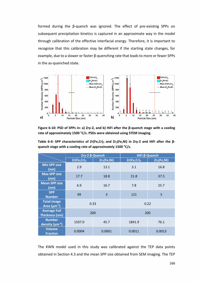
166

formed during the β-quench was ignored. The effect of pre-existing SPPs on

subsequent precipitation kinetics is captured in an approximate way in the model

through calibration of the effective interfacial energy. Therefore, it is important to

recognize that this calibration may be different if the starting state changes, for

example, due to a slower or faster β-quenching rate that leads to more or fewer SPPs

in the as-quenched state.

Figure 6-10: PSD of SPPs in: a) Zry-2, and b) HiFi after the β-quench stage with a cooling

rate of approximately 1500 °C/s. PSDs were obtained using STEM imaging.

Table 6-4: SPP characteristics of Zr(Fe,Cr)2 and Zr2(Fe,Ni) in Zry-2 and HiFi after the β-

quench stage with a cooling rate of approximately 1500 °C/s.

Zry-2 β-Quench HiFi β-Quench

Zr(Fe,Cr)2 Zr2(Fe,Ni) Zr(Fe,Cr)2 Zr2(Fe,Ni)

Min SPP size (nm)

2.9 13.1 3.1 16.8

Max SPP size (nm)

17.7 18.8 21.8 37.5

Mean SPP size (nm)

6.9 16.7 7.8 25.7

SPP Number

99 3 121 5

Total Image Area (μm-2)

0.33 0.22

Average Foil Thickness (nm)

200 200

Number density (µm-3)

1507.0 45.7 1841.9 76.1

Volume Fraction

0.0004 0.0001 0.0011 0.0013

The KWN model used in this study was calibrated against the TEP data points

obtained in Section 4.3 and the mean SPP size obtained from SEM imaging. The TEP

167

data points of interest are those that correspond to the onset of SPP coarsening. At

this point, it is assumed that the equilibrium volume fraction has been approximately

reached. This provides a calibration point for comparison with the model. For Zry-2,

this was obtained after 20 hr at 600 °C and after 2 hr at 700 °C. For HiFi, SPP

coarsening starts after 10 hr and 1 hr at 600 °C and 700 °C respectively. The PSDs of

both SPP types at these heat treatment temperatures and times are displayed in

Figure 6-11. The mean SPP size is obtained from Figure 6-11. The error bars on the

red histogram bars and cyan histogram bars show the standard error of the Zr(Fe,Cr)2

number density and Zr2(Fe,Ni) number density respectively. The error bar on the

horizontal red line and on the horizontal orange line are the standard errors of the

mean Zr(Fe,Cr)2 size and mean Zr2(Fe,Ni) size respectively. The class width was

determined using Equation 4-6 from Gros and Wadier [107].It is apparent that while

the mode size of the SPPs has increased significantly during the heat treatment,

which in turn increases the precipitate volume fraction, the number density of SPPs

drastically reduces. This suggests that the small SPPs formed during the β-quench

have experienced considerable dissolution. Many of these small particles probably

dissolved during the heat up to the isothermal heat treatment since they will be

below the critical radius at the isothermal temperature. Other particles will dissolve

by classical coarsening, which the TEP suggests has become well established under

the conditions used to produce the PSDs shown in Figure 6-11.

168

Figure 6-11: PSDs of Zr(Fe,Cr)2 and Zr2(Fe,Ni) in β-quenched Zry-2, subsequently

isothermally heat treated at: a) 600 °C / 20 hr, and b) 700 °C / 2hr. PSDs are also shown of

SPPs in β-quenched HiFi, isothermally heat treated at: c) 600 °C / 10 hr, and d) 700 °C / 1 hr.

PSDs were obtained using SEM imaging.

6.4.1 Effective Interfacial Energy

The effective interfacial energy parameter influences the nucleation rate at all

temperatures and influences the temperature sensitivity of the nucleation rate while

the 𝛸n parameter only influences the nucleation rate at all temperatures equally.

Therefore, the fitting process can arrive at a unique combination of these parameters

by first adjusting the effective interfacial energy to give the correct temperature

sensitivity before then adjusting 𝛸n to refine the fit for both temperatures. This

procedure was followed in the present work.

The model was calibrated against TEP and mean SPP size data points obtained in

isothermally heat treated Zry-2. As an initial starting point, the effective interfacial

energy value of Massih and Jernkvist [151] and Robson [150] was trialled for both

precipitate types. This value is 0.25 J/m2. The value was then adjusted to obtain the

correct temperature sensitivity of the model, since the interfacial energy term

controls how sensitive the kinetics are to changes in temperature [132]. Setting the

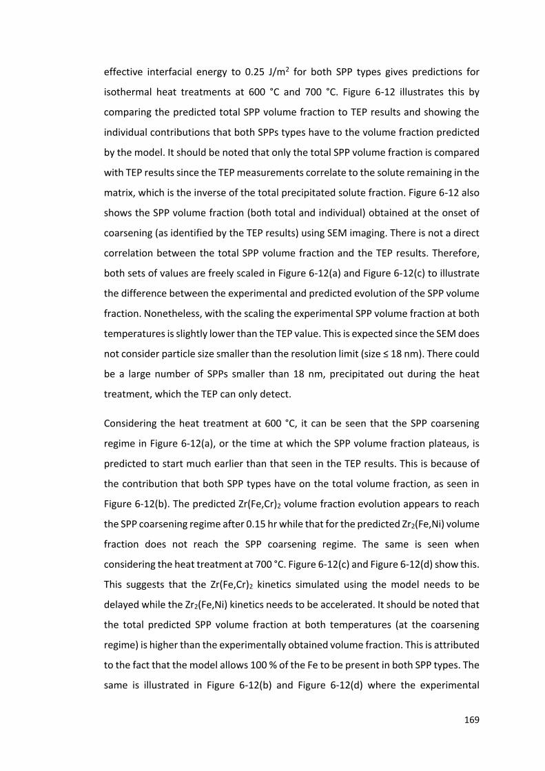
169

effective interfacial energy to 0.25 J/m2 for both SPP types gives predictions for

isothermal heat treatments at 600 °C and 700 °C. Figure 6-12 illustrates this by

comparing the predicted total SPP volume fraction to TEP results and showing the

individual contributions that both SPPs types have to the volume fraction predicted

by the model. It should be noted that only the total SPP volume fraction is compared

with TEP results since the TEP measurements correlate to the solute remaining in the

matrix, which is the inverse of the total precipitated solute fraction. Figure 6-12 also

shows the SPP volume fraction (both total and individual) obtained at the onset of

coarsening (as identified by the TEP results) using SEM imaging. There is not a direct

correlation between the total SPP volume fraction and the TEP results. Therefore,

both sets of values are freely scaled in Figure 6-12(a) and Figure 6-12(c) to illustrate

the difference between the experimental and predicted evolution of the SPP volume

fraction. Nonetheless, with the scaling the experimental SPP volume fraction at both

temperatures is slightly lower than the TEP value. This is expected since the SEM does

not consider particle size smaller than the resolution limit (size ≤ 18 nm). There could

be a large number of SPPs smaller than 18 nm, precipitated out during the heat

treatment, which the TEP can only detect.

Considering the heat treatment at 600 °C, it can be seen that the SPP coarsening

regime in Figure 6-12(a), or the time at which the SPP volume fraction plateaus, is

predicted to start much earlier than that seen in the TEP results. This is because of

the contribution that both SPP types have on the total volume fraction, as seen in

Figure 6-12(b). The predicted Zr(Fe,Cr)2 volume fraction evolution appears to reach

the SPP coarsening regime after 0.15 hr while that for the predicted Zr2(Fe,Ni) volume

fraction does not reach the SPP coarsening regime. The same is seen when

considering the heat treatment at 700 °C. Figure 6-12(c) and Figure 6-12(d) show this.

This suggests that the Zr(Fe,Cr)2 kinetics simulated using the model needs to be

delayed while the Zr2(Fe,Ni) kinetics needs to be accelerated. It should be noted that

the total predicted SPP volume fraction at both temperatures (at the coarsening

regime) is higher than the experimentally obtained volume fraction. This is attributed

to the fact that the model allows 100 % of the Fe to be present in both SPP types. The

same is illustrated in Figure 6-12(b) and Figure 6-12(d) where the experimental

170

Zr(Fe,Cr)2 volume fraction is less than that predicted using the model though the

evolution of the predicted SPP volume fraction is subject to change when the model

is calibrated.

Figure 6-12: SPP volume fraction of Zry-2 isothermally heat-treated at 600 °C where: a)

shows the comparison between TEP results, the un-calibrated simulated total SPP volume

fraction, and total SPP volume fraction obtained from SEM imaging after a 600 °C / 20 hr

heat treatment (where the TEP and total SPP volume fraction axes are freely scaled), and

b) shows the un-calibrated simulated volume fraction of both SPP types in addition to

experimentally obtained SPP volume fractions. The SPP volume fraction of Zry-2

isothermally heat-treated at 700 °C is presented where: c) shows the comparison between

TEP results, the un-calibrated simulated total SPP volume fraction, and total SPP volume

fraction obtained from SEM imaging after a 700 °C / 20 hr heat treatment (where the TEP

and total SPP volume fraction axes are freely scaled), and d) shows the un-calibrated

simulated volume fraction of both SPP types in addition to experimentally obtained SPP

volume fractions.

The simulations suggest that the interfacial energy of Zr(Fe,Cr)2 particles needs to

increase in order to delay the time taken for the onset of SPP coarsening. The effect

that different interfacial energy values have on the evolution of Zr(Fe,Cr)2

characteristics is displayed in Figure 6-13 when a 700 °C / 10 hr isothermal heat

treatment is simulated. The vertical line in each plot shows the time at 2 hr (i.e. the

171

time taken to reach the onset of coarsening identified when β-quenched Zry-2 is heat

treated at 700 °C). Increasing the interfacial energy has the effect of increasing mean

particle radius in Figure 6-13(a) [132]. Here, the coarsening regime dissolves smaller

particles and the nucleation of new particles is stopped. Figure 6-13(b) shows that an

increase in interfacial energy leads to a lower initial nucleation rate. This is consistent

with Equation 2-13 where an increase in interfacial energy, present in the critical free

energy term in the exponential, results in a lower nucleation rate. The nucleation

rate at higher interfacial energy values drops off towards zero later than that with

lower interfacial energy values due to the slower kinetics since the supersaturated

solute remaining in the matrix (which controls the driving force) falls more slowly.

When particles nucleate, the system experiences a reduction in solute concentration

in the matrix. Particles with a higher interfacial energy nucleate with a lower number

density than particles with a lower interfacial energy. When this solute concentration

gets too low, the driving force for nucleation reduces to effectively zero. This in turn

increases the critical particle size and reduces the nucleation rate [128]. Hence, if

particles have a higher interfacial energy, the nucleation rate drops off towards zero

less rapidly. The changes in solute concentration in the matrix and particle volume

fraction, shown in Figure 6-13(c) and Figure 6-13(d) respectively, with time are

affected by changes to the critical particle radius, nucleation rate and growth rate.

The higher interfacial energy has the effect of slowing down the reduction of solute

concentration in the matrix and thus slows down the evolution of the particle volume

fraction. This suggests that a higher interfacial energy, than that used previously, was

required for the kinetics of Zr(Fe,Cr)2 in Zry-2. From this, the interfacial energy of

Zr(Fe,Cr)2 was adjusted to 0.28 J/m2. Applying larger values of the interfacial energy,

with the combination of the calibration with the nucleation site density, leads to

further delays to the precipitation kinetics.

172

Figure 6-13: Predicted evolution of Zr(Fe,Cr)2 characteristics in Zry-2 with time, for varying

particle interfacial energy values, when subject to a 700 °C / 10 hr heat treatment with: a)

mean particle radius, b) nucleation rate, c) mean solute concentration in the matrix, and

d) volume fraction. The vertical line in each plot shows the time at 2 hr (i.e. the time taken

to reach the onset of coarsening identified when β-quenched Zry-2 is heat treated at

700 °C).

The infinitesimal increase in predicted Zr2(Fe,Ni) volume fraction at both

temperatures in Figure 6-12 result from the high particle interfacial energy used in

the simulation. Using the same analysis performed on the effect of interfacial energy

on Zr(Fe,Cr)2 kinetics, the interfacial energy of Zr2(Fe,Ni) was adjusted to 0.11 J/m2.

6.4.2 Nucleation Site Density

The value of the fitting parameter, 𝛸n, used initially was 5.00 × 10−7 as this value

had previously been used for the simulation of SPP kinetics in Zry-4 [150]. The

effective site density parameter is a function of alloy and dominant nucleating

feature (when nucleation is heterogeneous). This parameter therefore was adjusted

to give the best fit to the kinetics at both temperatures for the present case where

grain boundary precipitation is considered dominant. Figure 6-14 illustrates the

173

effect that different nucleation site density values have on the evolution of Zr(Fe,Cr)2

characteristics in Zry-2 when a 700 °C / 10 hr isothermal heat treatment is simulated.

The vertical line in each plot shows the time at 2 hr (i.e. the time taken to reach the

onset of coarsening identified when β-quenched Zry-2 is heat treated at 700 °C).The

particle interfacial energy for Zr(Fe,Cr)2 is 0.28 J/m2.

Figure 6-14: Predicted evolution of Zr(Fe,Cr)2 characteristics with time, for varying

nucleation site density values, when subject to a 700 °C / 10 hr heat treatment with: a)

mean particle radius, b) nucleation rate, c) mean solute concentration in the matrix, and

d) volume fraction. The vertical line in each plot shows the time at 2 hr (i.e. the time taken

to reach the onset of coarsening identified when β-quenched Zry-2 is heat treated at

700 °C).

A reduction in nucleation site density leads to a lower initial nucleation rate, and has

the effect of slowing down the reduction of solute concentration in the matrix and

thus slows down the evolution of the particle volume fraction. This in turn affects the

simulated mean particle radius which is generally larger with decreasing nucleation

site density. The best fit to the precipitation kinetics was found when 𝛸n was reduced

to 5.00 × 10−11 since the mean particle radius and the onset of SPP coarsening

(identified with the simulated volume fraction) are closest to that seen in the

174

experimental results for the same heat treatment condition. The modification to this

parameter reflects that only grain boundary precipitation is considered in the model.

Using the same analysis performed on the effect of nucleation site density on

Zr(Fe,Cr)2 kinetics, the 𝛸n used for Zr2(Fe,Ni) was adjusted to 5.00 × 10−13.

6.4.3 Comparison with Experimental Data

Predictions of the evolution of SPPs in Zry-2, isothermally heat treated at 600 °C and

700 °C, are compared against experimental data obtained using TEP and SEM

imaging. Figure 6-15(a) and Figure 6-15(b) illustrate how the predicted evolution of

the total volume fraction at 600 °C and 700 °C respectively are compared with

measured TEP data. As mentioned in Section 6.4.1, there is not a direct correlation

between the total SPP volume fraction and the TEP results and both sets of values

are freely scaled in Figure 6-15(a) and Figure 6-15(b). The trends from both

predictions of the total SPP volume fraction are in good agreement with the TEP

datasets, especially in capturing the time at which coarsening is predicted to become

dominant in both cases (the TEP and volume fraction plateau). The main difference

shown here is that the predicted total SPP volume fraction is approximately double

than that obtained experimentally at the onset of SPP coarsening. As mentioned

previously, this is attributed to the fact that the model assumes that the Fe is not

shared between the two SPP types and allows 100 % of the Fe to be present in both

SPP types (Section 6.2.1). An implication of this is that it is unknown whether the

model has been fully calibrated to the experimental TEP and SEM measurements.

Another approach to model calibration is to look at the comparisons between the

mean particle radius obtained both experimentally and by the model. Figure 6-15(c)

and Figure 6-15(d) show this at 600 °C and 700 °C respectively. It should be noted

that only one mean radius point is present at each temperature since the process of

performing experimental size distribution analysis on a number of heat treatment

conditions is extremely time consuming. The intention is to only confirm that the

KWN model generates reasonable predictions of the particle radius. Nonetheless, it

can be seen that at the heat treatments at which the SEM imaging were taken

(600 °C / 20 hr and 700 °C / 2 hr), the model is in good agreement with experimental

175

mean SPP radius. The mean particle radius also reaches a steady state value with the

exception of the mean Zr2(Fe,Ni) radius in Figure 6-15(d). Nonetheless, this suggests

that SPP nucleation has ceased and the plateau occurs when precipitate growth and

dissolution are in balance – this is typical in the regime where coarsening is becoming

established and where there is no overlap between nucleation and coarsening

regimes [132].

Figure 6-15: Predicted evolution of the total SPP volume fraction in Zry-2 compared with

TEP data and total SPP volume fraction obtained using SEM imaging at: a) 600 °C, and b)

700 °C. The predicted mean radius of Zr(Fe,Cr)2 and Zr2(Fe,Ni) is also compared to that

obtained at the onset of SPP coarsening using the SEM at: c) 600 °C, and d) 700 °C.

6.5 Application of KWN Model

6.5.1 Modelling SPP Kinetics in HiFi

The calibrated model has been applied to predict the kinetics of both SPP types in

HiFi assuming the same set of calibration values can also be applied to this alloy. This

is reasonable, since apart from the differences in composition, the other features of

the microstructure are similar in both alloys. The input parameters used previously

remain the same with the exception of the solute concentration in the matrix, 𝑥b.

176

This parameter had to be modified to take into consideration the increase in Fe from

0.18 wt% to 0.40 wt% in HiFi. Figure 6-16(a) and Figure 6-16(b) demonstrate how the

predicted evolution of the total SPP volume fraction at 600 °C and 700 °C compares

with the TEP evolution of HiFi at these temperatures and the total SPP volume

fraction (using SEM imaging) obtained at the onset of coarsening (as identified by the

TEP results). As with Figure 6-15, the predicted total SPP volume fraction is

approximately twice as large than that seen experimentally. Nevertheless a good

agreement is seen between the trends of the TEP results and the predicted total SPP

volume fraction at times where the latter is constant. Deviations between the

predicted volume fraction and the TEP datasets are seen at times less than 10 hr in

Figure 6-16(a). The trend from the TEP data points suggests the evolution of the SPP

volume fraction is more delayed than that predicted by the model. This could result

from microstructural differences between Zry-2 and HiFi (e.g. the change in the

number of available nucleation sites). Figure 6-16(c) and Figure 6-16(d) depict mean

radius predictions from the model compared against the mean SPP radius measured

using SEM imaging at 600 °C and 700 °C respectively. As with that in Figure 6-15, only

one mean radius point is present at each temperature. The model predicts that the

mean radius of both SPP types reaches a steady state value at the heat treatments

at which the SEM imaging was taken (600 °C / 10 hr and 700 °C / 1 hr). However, with

the exception of the mean Zr2(Fe,Ni) radius in Figure 6-16(d), these data points are

not at the onset of the plateau suggesting the model predicts that the coarsening

regime starts earlier than expected in HiFi.

The predicted mean Zr(Fe,Cr)2 radius is in good agreement with that obtained using

SEM imaging while the predicted mean Zr2(Fe,Ni) radius is lower than that seen using

SEM imaging with this being more prominent in Figure 6-16(c). However, at both

temperatures the predicted mean radius is within 50% of the measured value. These

predictions could be improved with small changes to the calibration parameters, but

this was not the purpose of the present calculation. For example, since HiFi has a

higher Fe content than Zry-2, the size of prior β-grains after β-quenching is slightly

larger (since Fe is a β-Zr stabiliser). Subsequent thermomechanical processing leads

to HiFi having slightly larger grains than Zry-2. As a result, if considering grain

177

boundary precipitation only, there are fewer potential nucleation sites for SPP

nucleation i.e. the 𝛸n parameter for both SPP types should be smaller than that used

for Zry-2 precipitation. Nevertheless, the key point is that even without re-

calibration, the model developed for Zry-2 can be directly applied to HiFi and gives

approximately reasonable predictions of the kinetics. This suggests that there is not

a fundamental difference in the precipitation behaviour in the two alloys, but rather

a difference in the balance of phases as demonstrated in Figure 6-16.

Figure 6-16: Predicted evolution of the total SPP volume fraction in HiFi compared with TEP

data and total SPP volume fraction obtained using SEM imaging at: a) 600 °C, and b) 700 °C.

The predicted mean radius of Zr(Fe,Cr)2 and Zr2(Fe,Ni) is also compared to that obtained at

the onset of SPP coarsening using the SEM at: c) 600 °C, and d) 700 °C.

6.5.2 Application to Industrial Processing

The calibrated model was used to predict the evolution of SPP characteristics of both

SPP types in Zry-2 throughout the thermal history used in the thermomechanical

processing of cladding tubes. Figure 6-17 illustrates this where the thermal history

consists of a hot anneal, which would be prior to hot extrusion, an air cool with an

average cooling rate of 4 °C/s, an intermediate anneal with a heating and cooling rate

of 3 °C/s, and a final anneal with a heating and cooling rate of 3 °C/s. It should be

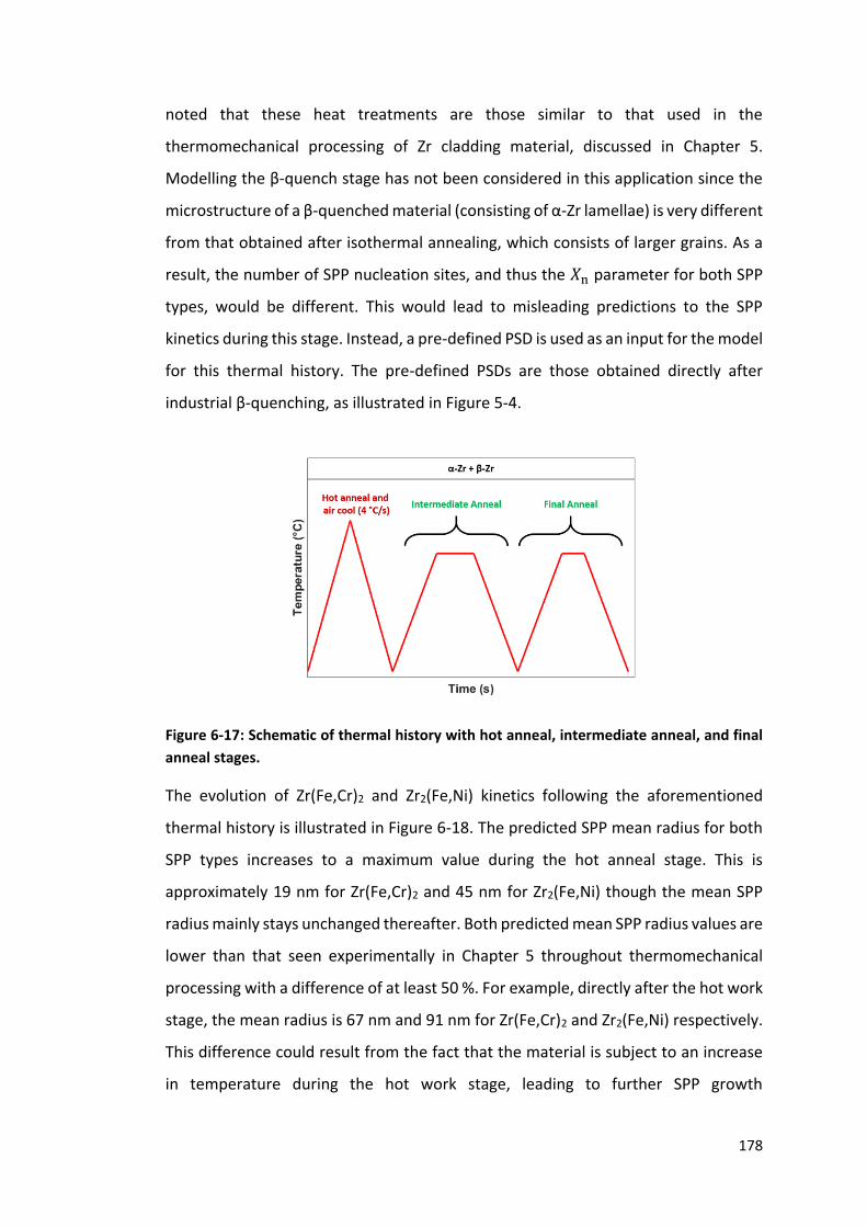
178

noted that these heat treatments are those similar to that used in the

thermomechanical processing of Zr cladding material, discussed in Chapter 5.

Modelling the β-quench stage has not been considered in this application since the

microstructure of a β-quenched material (consisting of α-Zr lamellae) is very different

from that obtained after isothermal annealing, which consists of larger grains. As a

result, the number of SPP nucleation sites, and thus the 𝛸n parameter for both SPP

types, would be different. This would lead to misleading predictions to the SPP

kinetics during this stage. Instead, a pre-defined PSD is used as an input for the model

for this thermal history. The pre-defined PSDs are those obtained directly after

industrial β-quenching, as illustrated in Figure 5-4.

Figure 6-17: Schematic of thermal history with hot anneal, intermediate anneal, and final

anneal stages.

The evolution of Zr(Fe,Cr)2 and Zr2(Fe,Ni) kinetics following the aforementioned

thermal history is illustrated in Figure 6-18. The predicted SPP mean radius for both

SPP types increases to a maximum value during the hot anneal stage. This is

approximately 19 nm for Zr(Fe,Cr)2 and 45 nm for Zr2(Fe,Ni) though the mean SPP

radius mainly stays unchanged thereafter. Both predicted mean SPP radius values are

lower than that seen experimentally in Chapter 5 throughout thermomechanical

processing with a difference of at least 50 %. For example, directly after the hot work

stage, the mean radius is 67 nm and 91 nm for Zr(Fe,Cr)2 and Zr2(Fe,Ni) respectively.

This difference could result from the fact that the material is subject to an increase

in temperature during the hot work stage, leading to further SPP growth

179

(Section 5.4.1). However, the experimental PSDs that were measured using SEM

imaging do not consider the contribution that SPPs smaller than 18 nm in size have

on the mean SPP size. Therefore, the model is more likely to be closer to realist than

illustrated. The predicted SPP number density in Figure 6-18(b) remains unchanged

at very high values throughout the thermal history, much higher than that seen in

Chapter 5. Figure 6-18(c) suggests that the majority of the SPP nucleation has taken

place during the β-quench stage since nucleation for Zr(Fe,Cr)2 is complete during the

hot anneal stage. Zr2(Fe,Ni) nucleation is fully complete during the intermediate

stage since a small number density of Zr2(Fe,Ni) particles are formed in the β-quench

and hot anneal stages. The Zr2(Fe,Ni) nucleation rate is not complete during the hot

anneal stage since the particle’s interfacial energy is lower than that for Zr(Fe,Cr)2

particles. This is illustrated in Figure 6-13(b) where particles with a lower interfacial

energy complete nucleation earlier than those with a larger interfacial energy. The

main changes in the SPP volume fraction and the mean solute concentration in the

matrix are also predicted to take place during the hot anneal stage. Here, the SPP

volume fraction reaches the equilibrium value of 0.008 and 0.0106 for Zr(Fe,Cr)2 and

Zr2(Fe,Ni) respectively. At this point, SPP coarsening is the dominant regime. It should

be noted that the SPP volume fraction deviates from the equilibrium volume fraction

in the subsequent anneal stages due to the changes in temperature during the

heating and cooling steps. The predicted SPP volume fractions are much larger than

that seen experimentally. This is attributed to the fact that the model only considers

the SPP types as separate systems and allows 100 % of the Fe to be present in both

SPP types (which does not happen in reality). The mean solute concentration in the

matrix reduces to a minimum value and plateaus. These trends suggest that the onset

of SPP coarsening takes place during the hot anneal stage.

The predicted PSDs of SPP types at the end of the simulated thermal history is

displayed in Figure 6-18(f). It is observed that the predicted PSDs after the final

anneal are skewed to much smaller sizes. This is indicated by the fact that the

predicted mean SPP radius is at least 40 % smaller than that seen experimentally and

that the predicted peak SPP number density in the PSDs are much higher than that

seen in the experimental PSDs (Figure 5-7). As mentioned previously, the predicted

180

mean SPP size may be closer than that seen experimentally since SEM imaging does

not consider the presence of small SPPs. The much larger peak number density

observed in Figure 6-18(f) can be correlated to the fact that this model assumes that

100 % of the Fe present in the system goes to both types of SPP. In reality, Fe is shared

between the SPPs and thus can affect SPP kinetics. In addition to this, the differences

between the experimental value and that predicted using the model can also be

attributed to the fact that deformation effects have not been introduced into the

model. Hot work has the tendency to increase material temperature and break up

the microstructure, allowing a larger proportion of SPPs to nucleate and grow within

the grain interior. Further, as discussed in Section 5.4.2, cold pilgering has the effect

of shearing large particles into numerous smaller particles. This has the tendency to

shift the PSD to smaller sizes and broaden the PSD slightly. Further, the increased

dislocation density introduced as a result of the deformation increases the diffusion

of solutes. This can lead to accelerated growth of SPPs during the subsequent anneal

stages. Therefore, multiple cold work and anneal stages have the effect of reducing

the peak SPP value while broadening the PSD. Cold work also breaks up the

microstructure further. This in turn affects the nucleation rate and diffusivity of

solutes, both of which have remained constant in the model. Nonetheless, the key

point is that the model is capable of providing indications of the behaviour that both

SPPs types in Zry-2 have when subject to a thermal history.

181

Figure 6-18: Evolution of both SPP types in Zry-2 throughout a simulated thermal history

where the following characteristics are shown: a) mean particle radius, b) particle number

density, c) particle nucleation rate, d) mean solute concentration in the matrix, e) SPP

volume fraction and equilibrium SPP volume fraction, and f) the PSD after the final anneal.

The hot anneal, intermediate, and final anneal stages are abbreviated to: HA, IA, and FA.

6.6 Summary

This chapter introduced a physical model based on classical nucleation, growth, and

coarsening theories that has been adapted to predict the precipitation kinetics of

SPPs in Zry-2. The particle interfacial energy and the nucleation site density have

been adjusted accordingly to calibrate the model against experimental datasets from

the TEP and SEM imaging for both SPP types. A good agreement is seen between the

182

predicted volume fraction and mean particle size to that observed experimentally

when isothermally heat-treated at 600 °C and 700 °C. The main difference between

the un-calibrated model (Figure 6-12) and the calibrated model (Figure 6-15) is that

the former was only capable of predicting the precipitation of Zr(Fe,Cr)2. The un-

calibrated model showed that the predicted total SPP volume fraction is similar to

the total SPP volume fraction observed experimentally since the model did not

correctly predict the evolution of Zr2(Fe,Ni) particles. Adjustments to solute diffusion,

interfacial energy, and nucleation site density in the modified model ensures that the

evolution of Zr2(Fe,Ni) particles is predicted accurately. In addition to this, the

calibrated model delays the predicted onset of SPP coarsening (plateau in predicted

total SPP volume fraction) such that the trends are similar to that seen in the

experimental TEP results (Section 4.3). Figure 6-12 and Figure 6-15 also shows the

SPP volume fraction experimentally obtained using SEM imaging. The main

difference between the predicted and experimental SPP volume fraction (at the

onset of SPP coarsening) is that the predicted total SPP volume fraction is

approximately double than that obtained experimentally at the onset of SPP

coarsening. This is because the model allows 100 % of the Fe to be present in both

SPP types (Section 6.2.1).

SPP kinetics were also predicted in HiFi where the kinetics of both SPP types provided

a good agreement, especially with the onset of SPP coarsening identified by the

experimental TEP data points. As with that seen when predicting the SPP kinetics in

Zry-2, the predicted SPP volume fraction for HiFi is larger than that seen

experimentally. The predicted mean Zr(Fe,Cr)2 radius also is in good agreement with

the experimental data point while the predicted mean Zr2(Fe,Ni) radius is

consistently less than that obtained experimentally. These predictions could be

improved with small changes to the calibration parameters, especially to the

nucleation site density where the difference in composition can have an effect on the

microstructure. The model has also provided an insight into SPP kinetics in Zry-2

throughout a thermal history used in processing of cladding material. This illustrates

that nucleation and growth regimes are dominant prior to the hot anneal stage. The

SPP coarsening regime is dominant during the hot anneal stage and continues to

183

dominate throughout the thermal history where the SPP volume fraction and solute

concentration in the matrix reach a plateau. This is consistent to that seen in

Chapter 5. The mean SPP radius and the final PSD after the thermal history are both

lower than that seen experimentally since SEM imaging does not capture the effect

that SPPs smaller than 18 nm have on the size distribution. In addition, deformation

is absent in the model, which would enable higher solute diffusion and enable smaller

SPPs due to larger SPPs breaking up. Further, the SPP number density is much higher

than that seen in Chapter 5 since it is assumed that Fe is not shared between the

SPPs. Despite this, the model predictions are within 50 % of that produced

experimentally and therefore is capable of providing an indication of the SPP kinetics

of Zr(Fe,Cr)2 and Zr2(Fe,Ni) in Zry-2 when subject to a thermal history.

This model is different to other kinetics models that have been developed to simulate

precipitation in Zr alloys. Previously, only Zr(Fe,Cr)2 has been simulated in Zry-2 since

the properties of this SPP type has been identified in literature [41, 151] while that

for Zr2(Fe,Ni) has not determined thus far. By predicting the evolution of SPP kinetics

of both Zr2(Fe,Ni) and Zr(Fe,Cr)2, in its current state, this new model can be used by

industry to predict the behaviour of SPPs when subject to a thermal history. For

example, the heat treatments can be modified if a specific PSD is required. This in

turn can be used to optimise Zr alloy performance either in-reactor or in autoclave

testing. Significant cost savings can therefore be made by using the kinetics model

instead of using thermomechanical processes, such as furnaces, to optimise PSDs.

This is key since the main objective of Zr alloy research is to prolong their lifetime in

the reactor environment while reducing costs. In addition to this, the kinetics model

can be adapted to be predict multiple precipitation in other alloy systems such as

HSLA steel (with Nb(C,N)-, AlN-, and MnS-precipitates) [152], and 2xxx Al series

alloys [194]. In doing so, modifications are required for the model’s input parameters

(Section 6.3) to accommodate for the precipitate properties. As with this study, the

model will also require calibration against experimental data points. Nonetheless,

this demonstrates the model’s flexibility in predicting multiple precipitation in alloy

systems.

184

7 Conclusions

The aim of this project was to characterize SPPs in both Zry-2 and the novel high Fe-

alloy, HiFi and model the SPP kinetics. The Laves phase, Zr(Fe,Cr)2, and the tetragonal

phase, Zr2(Fe,Ni), are SPPs that were studied. These SPPs were distinguished and

characterized using different experimental techniques. The evolution of the SPPs

throughout the thermomechanical processing of Zr cladding tubes was identified

using electron microscopy. In addition, the effect of certain processing stages on SPP

evolution was analysed. SPP kinetics were also predicted using a modified version of

the KWN model. This model was calibrated against experimental data points. The

conclusions from this study are as follows:

7.1 SPP Characterization Techniques

The SPPs in HiFi were identified using EBSD in the SEM where the two SPP types in

this alloy are the same as that in Zry-2. These SPPs can also be distinguished using

low keV EDX and BSE imaging in the SEM. Compositional contrast is attained using

BSE imaging and thus is mainly used to obtain statistical data on a large number of

SPPs. Reliable PSDs are produced using SEM imaging since a large area can be

analysed. SEM imaging resolution is limited to not only the beam conditions but also

the sample preparation technique which leads to the formation of a passive oxide

layer. This oxide layer can adversely affect SPP compositional contrast and also hide

smaller particles from detection. Resolution limitations are overcome by using

(S)TEM imaging. However, fewer SPPs are sampled and less reliable PSDs are

generated since a smaller sample volume is examined. In addition, complications

arise in compositional contrast imaging using STEM-HAADF due to mass-thickness

contrast, and SPP identification via diffraction due to small SPPs being surrounded by

thick regions of α-Zr matrix. Despite this, superior elemental analysis can be

obtained, leading to SPP chemistry analysis.

SPPs can also be characterized indirectly using techniques such as DSC and TEP. The

DSC technique has the capability of measuring endothermic peaks related to SPP

dissolution, which in turn provides an indication of the SPP volume fraction.

185

Furthermore, the SPP dissolution temperature can be measured. β-quenched

material (supplied by Sandvik AB) was tested, leading to measurements where only

one enthalpic peak is present. Deconvolution of enthalpic peaks cannot be easily

achieved since the SPP dissolution temperatures are too close together. Therefore,

the DSC is not a suitable technique for tracking SPP precipitation kinetics.

TEP is sensitive to microstructural changes including changes in solute concentration

in the matrix when the alloys are subject to heat treatments. The heat treated

material were compared against a β-quenched reference with a cooling rate of

approximately 1500 °C/s. As the SPPs form during the heat treatments, the solute

concentration reduces and in turn the TEP value increases. Thereafter, the TEP value

reaches a plateau, indicating a steady-state level of solute concentration in the matrix

and thus a constant SPP volume fraction. It is observed that heat-treated HiFi

produces higher TEP values than that for Zry-2 for the same heat treatment. This

results from the increased precipitation of SPPs in HiFi, and thus a larger SPP volume

fraction. Irrespective of this, the time for the completion of precipitation, or the time

at which particle coarsening takes place, can be determined. Therefore, TEP is a

suitable technique for tracking the overall precipitation kinetics of SPPs.

7.2 SPP Evolution throughout Thermomechanical

Processing

SEM imaging was employed to determine the difference in SPP characteristics

between Zry-2 and HiFi where a similar SPP number density was observed though

SPPs in HiFi are generally larger. Throughout thermomechanical processing, it was

observed that the total SPP volume fraction starts at 0.004 and 0.009 in Zry-2 and

HiFi respectively at the industrial β-quench stage. STEM imaging was utilised, leading

to the discovery of a large number density of Zr(Fe,Cr)2 particles in both alloys as well

as the formation of SPPs on dislocations as well as grain boundaries.

SPP characteristics in subsequent stages were analysed using SEM imaging. For both

alloys, the volume fraction of both SPP types remained relatively constant

(accounting for error), suggesting that SPP coarsening is the dominant regime after

β-quenching. The mean SPP size decreases gradually throughout thermomechanical

186

processing while the SPP number density increases. The difference between the two

alloys is that HiFi has a larger volume fraction of SPPs and also has a larger mean SPP

size though the SPP number density seems to be similar. The hot work stage increases

the SPP volume fraction, leading to an excess of SPPs in the system. The hot work

stage also leads to a deformed microstructure that produces a more distribution of

SPPs than that observed during the β-quench stage. Cold pilgering has the effect of

reducing the mean SPP size and increasing the SPP number density. This is attributed

to the fact that larger SPPs are being sheared by the cold pilgering process into

smaller SPPs. Annealing on the other hand leads to larger mean SPP sizes and a

reduced particle number density. This results from the diffusion of solutes from

particle to particle, leading to the dissolution of smaller particles and the growth of

larger particles (the coarsening process). From STEM analysis, SPPs in the pilger and

anneal stages tend to have a homogeneous distribution of solutes. HiFi generally has

SPPs with a larger solute ratio than that in Zry-2 (due to the higher Fe content).

Nonetheless, the change in solute ratios between the pilger and anneal stage is

minimal. This suggests that limited diffusion is present between the stages though

with further processing, this may be significant since this leads to changes in SPP

volume fraction and solute concentration in the matrix. As a result, corrosion

performance of the product can be optimised.

7.3 Simulating SPP Kinetics in Zircaloy-2 and HiFi

SPP kinetics in both alloys were predicted using the KWN model, based on classical

nucleation theory. From the analysis in Chapter 4 and Chapter 5, the model was

modified to consider heterogeneous nucleation of spherical particles. The SPP and

solute characteristics were also modified from previous studies on precipitation

kinetics of SPPs in Zr alloys to consider the precipitation kinetics of Zr(Fe,Cr)2 and

Zr2(Fe,Ni). The undefined parameters are the effective particle interfacial energy and

the effective nucleation site density multiplication factor. These are used as

calibration parameters to fit the KWN model to experimental TEP data points (on

isothermally heat treated material) and mean SPP radius at the onset of coarsening.

The initial condition of the material was to assume a supersaturated solid solution

since the volume fraction of SPPs present in Zry-2 and HiFi, after a β-quench with a

187

cooling rate of 1500 °C/s, is miniscule. Model calibration was initially performed

against experimental Zry-2 data points where the TEP measurements were compared

against total SPP volume fraction and the mean SPP radius was to that predicted at

the onset of coarsening.

The calibrated model was applied to HiFi and compared to the experimental data

points. A very good agreement was seen between the TEP data and the total SPP

volume fraction. The predicted mean Zr(Fe,Cr)2 radius was is in good agreement with

the experimental data point though the predicted mean Zr2(Fe,Ni) radius is

consistently lower than that obtained experimentally with a difference of at least

30 %. This could result from the fact that the alloys have slightly different

microstructures and could be improved with small changes to the calibration

parameters, but this was not the purpose of the present calculation. Nonetheless,

the key point is that even without re-calibration, the model developed for Zry-2 can

be directly applied to HiFi, providing reasonable predictions.

The model was also applied to the thermal history used in industrial processing on

SPPs in Zry-2. The initial PSD for this simulation was defined by the PSD obtained at

the industrial β-quench stage seen in Chapter 5. Application of the thermal history

on the PSD shows that SPP nucleation and growth regimes are dominant until part-

way through the hot anneal stage. Thereafter, SPP coarsening initiates and the mean

SPP radius and volume fraction reach peak values while the mean solute

concentration in the matrix reaches a minimum value. The model does not include

the effect of SPP break up during the pilgering process or the co-precipitation of

particles observed experimentally. With further understanding of the mechanisms

controlling these processes, both effects could be included in the model and would

improve its accuracy. Despite this, the model is capable of providing an indication of

the SPP kinetics in Zry-2 when subject to a thermal history.

188

8 Future Work

Future projects as a continuation of this study can be focussed on the effects that

thermomechanical processing have on SPP characteristics and further development

of the SPP kinetics model.

8.1 Effect of Thermomechanical Processing on SPP

Characteristics

This study has explored how thermomechanical processing affects SPP

characteristics in Zry-2 and HiFi cladding material. Analysis thus far has concentrated

on the evolution of SPP volume fraction, mean size, number density, and PSD.

Another characteristic that can be measured is the change in solute concentration

from stage to stage. This is thought to take place due to the changes in SPP sizes

throughout processing and the very slight changes in SPP chemistry between the

pilger and anneal stages (though this is not measureable using STEM). This effect can

be investigated by creating matchsticks from the cladding material which then can

be used in the TEP. The changes in solute concentration will lead to changes in the

TEP, no matter how small the changes are. APT could also be used to complement

the TEP data by examining the quantity of solutes in the SPPs and the matrix. This

data, including that generated in the present study, can be correlated to the

corrosion performance and hydrogen pick-up data generated in industry for these

alloys. In turn, this has the potential to provide an insight into how thermomechanical

processing of Zr cladding tubes affects performance and can be optimised to improve

component lifetime in the reactor environment.

8.2 Quantity of Solutes in SPPs and Matrix

As mentioned above, the chemistries of the SPPs are subject to change. This in turn

affects the accuracy of the kinetics model developed in this study. For example,

Chapter 6 illustrates that the predicted SPP number density in Zry-2 (when subject to

a thermal history) remains at a very high number – 274 SPPs/μm-3 and 28 SPPs/μm-3

for Zr(Fe,Cr)2 and Zr2(Fe,Ni) respectively – though the experimental PSDs (after the

β-quench stage) show a total number density of approximately 1 SPP/μm-3. This

189

discrepancy between predicted and experimental PSDs can be minimised by

considering the quantity of solutes present in the SPPs. This is especially the case for

Fe where, for the purpose of this study, it was assumed that this alloying element is

not shared between the two SPP types. This also has an effect on the effective

diffusivities of (Fe+Cr) and (Fe+Ni) since these are dependent on the individual

diffusivity of Fe, Cr, and Ni. The diffusion of Cr and Ni in α-Zr grains are the rate

limiting factors since they are slower diffusers than Fe. Therefore, if the exact

chemistry of the SPPs in Zry-2 and HiFi (at different processing steps) are known, the

diffusion of (Fe+Cr) and (Fe+Ni) can be modified to reflect this. Elemental

quantification can be obtained by using APT on needle-shaped samples containing

SPPs. In addition, the quantity of solute in the matrix could be determined. This could

be applied to all stages of thermomechanical processing from the β-quench stage to

the final anneal stage to provide a detailed characterization of solute behaviour

during processing.

8.3 Modelling Zr2(Fe,Ni) kinetics

As seen in Chapter 6, some of the Zr2(Fe,Ni) characteristics have been approximated

due to the lack of experimental data in literature and inconsistencies in

thermodynamical simulations. This is prominent in the variable 𝑥aFe+Ni which defines

the concentration of (Fe+Ni) solutes in the matrix that are in equilibrium with the

Zr2(Fe,Ni). This variable requires a fully defined solvus line like that demonstrated by

Charquet et al. in the Zr-Fe-Cr system [40]. The solvus line in the Zr-Fe-Ni system

could be investigated by developing small quantities of material with varying

compositions of Fe and Ni. This material would then be subject to different heat

treatments (within the temperature range of 500 °C to 950 °C) which are then water

cooled. SEM and STEM analysis of the microstructure can be applied to detect the

presence of SPPs. From this, a more accurate representation of 𝑥aFe+Ni can be

determined.

190

8.4 Simulating the Effect of Deformation and Grain Growth

on SPP Kinetics

The hot work and cold pilger stages not only change the dimensions of the Zr tube

but also affect the microstructure. This leads to a homogeneous distribution of SPPs,

a broader PSD and grain growth (especially in the hot work stage). Throughout the β-

quench stage, SPPs are primarily formed on defects such as dislocations and grain

boundaries. With further processing, which includes deformation and grain growth,

SPPs are located both on grain boundaries and within the grain interior, the

proportion of which changes with each processing stage. In turn, an additional set of

parameters would need to be introduced to consider the effects that deformation

and grain growth have on SPP kinetics. These parameters would affect inputs factors

such as the solute diffusivity, and the effective nucleation site density since these

have to be adjusted with each processing stage. SEM imaging would have to be

implemented to determine how the proportion of grain interior to grain boundary

precipitation changes with each processing stage from the β-quench stage to the final

anneal stage. APT may also have to be used to understand the effect that the

increased dislocation density (from pilgering) has on solute diffusion during the

anneal stages and thus how SPP evolution is affected. This part of the study could be

used to determine how the solute diffusivity term changes between processing

stages. Further analysis could also enhance the understanding of how the diffusivity

of the individual solutes change with processing. This can lead improved input data

for solute diffusion.

191

9 References

[1] IEA and OECD, World Energy Outlook 2009. Paris: IEA, 2009.

[2] IEA, “World Energy Outlook,” 2019. [Online]. Available:

https://www.iea.org/weo/. [Accessed: 27-Aug-2019].

[3] Legislation.gov.uk, “Climate Change Act 2008,” 2008. [Online]. Available:

http://www.legislation.gov.uk/ukpga/2008/27/part/1/crossheading/the-

target-for-2050. [Accessed: 27-Aug-2019].

[4] BBC, “EDF to Keep Four UK Nuclear Plants Open for Years Longer,” 2016.

[Online]. Available: https://www.bbc.co.uk/news/business-35583740.

[Accessed: 27-Aug-2019].

[5] “Types of Reactor,” Nuclear Power for Everybody, 2019. [Online]. Available:

https://www.nuclear-power.net/nuclear-power-plant/reactor-types/.

[Accessed: 27-Aug-2019].

[6] S. E. Jensen and E. Nonbol, “Description of the Magnox Type of Gas Cooled

Reactor (MAGNOX),” Roskilde, 1998.

[7] ONR, “Report by HM Nuclear Installations Inspectorate on the results of

Magnox Long Term Safety Reviews (LTSRs) and Periodic Safety Reviews

(PSRs),” 2017.

[8] AECL, “CANDU 6 Technical Summary,” Ontario, 2005.

[9] V. G. Asmolov, “Development of the NPP Designs Based on the VVER

Technology.” Paris, 2009.

[10] IAEA, “Accident Analysis for Nuclear Power Plants with Graphite Moderated

Boiling Water RBMK Reactors,” Vienna, 2005.

[11] USDOE, “A Technology Roadmap for Generation IV Nuclear Energy Systems,”

2002.

[12] EcoWatch, “Interactive Map Details What You Need to Know About the

World’s Nuclear Power Plants,” 2016. [Online]. Available:

https://www.ecowatch.com/interactive-map-details-what-you-need-to-

know-about-the-worlds-nuclear-1882188367.html. [Accessed: 27-Aug-2019].

[13] L. Hallstadius, S. Johnson, and E. Lahoda, “Cladding for High Performance

Fuel,” Prog. Nucl. Energy, vol. 57, pp. 71–76, 2012.

[14] T. Andersson and G. Vesterlund, “Beta-Quenching of Zircaloy Cladding Tubes

192

in Intermediate or Final Size - Methods to Improve Corrosion and Mechanical

Properties,” in Zirconium in the Nuclear Industry: Fifth International

Symposium, 1982, pp. 75–95.

[15] T. Andersson and T. Thorvaldsson, “Nodular Corrosion Resistance of Zircaloy-

2 in Relation to Second-Phase Particle Distribution,” in Zirconium in the

Nuclear Industry: Seventh International Symposium, 1987, pp. 321–337.

[16] B. Cheng and R. B. Adamson, “Mechanistic Studies of Zircaloy Nodular

Corrosion,” in Zirconium in the Nuclear Industry: Seventh International

Symposium, 1987, pp. 387–416.

[17] R. M. Kruger, R. B. Adamson, and S. S. Brenner, “Effects of Microchemistry and

Precipitate Size on Nodular Corrosion Resistance of Zircaloy-2,” J. Nucl. Mater.,

vol. 189, no. 2, pp. 193–200, 1992.

[18] T. Kubo and M. Uno, “Precipitate Behaviour in Zircaloy-2 Oxide Films and its

Relevance to Corrosion Resistance,” in Zirconium in the Nuclear Industry: Ninth

International Symposium, 1991, pp. 476–498.

[19] G. Maussner, E. Steinberg, and E. Tenckhoff, “Nucleation and Growth of

lntermetallic Precipitates in Zircaloy-2 and Zircaloy-4 and Correlation to

Nodular Corrosion Behaviour,” in Zirconium in the Nuclear Industry: Seventh

International Symposium, 1987, pp. 307–320.

[20] A. R. Massih, M. Dahlbäck, M. Limbäck, T. Andersson, and B. Lehtinen, “Effect

of Beta-to-Alpha Phase Transition Rate on Corrosion Behaviour of Zircaloy,”

Corros. Sci., vol. 48, no. 5, pp. 1154–1181, 2006.

[21] D. Charquet, “Improvement of the Uniform Corrosion Resistance of Zircaloy-4

in the Absence of Irradiation,” J. Nucl. Mater., vol. 160, no. 2–3, pp. 186–195,

1988.

[22] K. Kakiuchi et al., “Role of Iron for Hydrogen Absorption Mechanism in

Zirconium Alloys,” in Zirconium in the Nuclear Industry: Fourteenth

International Symposium, 2004, vol. 1, no. 10, pp. 349–366.

[23] K. Kakiuchi et al., “Effect of Iron on Hydrogen Absorption Properties of

Zirconium Alloys,” J. Phys. Chem. Solids, vol. 66, pp. 308–311, 2005.

[24] K. Kakiuchi, K. Ohira, N. Itagaki, Y. Otsuka, Y. Ishii, and A. Miyazaki, “Irradiated

Behavior at High Burnup for HiFi Alloy,” J. Nucl. Sci. Technol., vol. 43, no. 9, pp.

1031–1036, 2006.

[25] K. Kataoka et al., “The Irradiation Performance and Experience of Advanced

Zirconium Alloy HiFi(R) in a Commercial BWR,” 2012.

193

[26] D. Benjamin, Metals Handbook. Properties and Selection: Nonferrous Alloys

and Pure Metals, 9th ed. Metals Park, Ohio: American Society for Materials,

1979.

[27] R. Adamson and P. Rudling, “IZNA-1 Special Topics Report: Manufacturing of

Zr alloys,” Ekbaken, 2004.

[28] I. Charit and K. L. Murty, “Creep Behaviour of Niobium-Modified Zirconium

Alloys,” J. Nucl. Mater., vol. 374, no. 3, pp. 354–363, 2008.

[29] N. Rao and V. Bangaru, “An Investigation of the Microstructures of Heat-

Treated Zircaloy-4,” J. Nucl. Mater., vol. 131, pp. 280–290, 1985.

[30] R. Krishnan and M. K. Asundi, “Zirconium Alloys in the Nuclear Industry,” in

Indian Academy of Sciences, 1981, vol. 4, pp. 41–56.

[31] D. O. Northwood, “The Development and Applications of Zirconium Alloys,”

Mater. Des., vol. 6, no. 2, pp. 58–70, 1985.

[32] H. G. Rickover, L. D. Geiger, and B. Lustman, “History of the Development of

Zirconium Alloys for Use in Nuclear Reactors,” 1975.

[33] J. Schemel, ASTM Manual on Zirconium and Hafnium. ASTM STP 639, American

Society for Testing and Materials, 1977.

[34] B. Lustman and F. Kerze, The Metallurgy of Zirconium. McGraw-Hill Book

Company, Inc, 1955.

[35] H. Q. Zhang, X. F. Wang, B. L. Wei, and H. Li, “Effect of Tooling Design on the

Cold Pilgering Behaviour of Zircaloy Tube,” Int. J. Adv. Manuf. Technol., vol. 92,

pp. 2169–2183, 2017.

[36] M. Ivermark, “Characterization of the Matrix Chemistry in Zirconium Alloys,”

University of Manchester, 2009.

[37] Y. H. Jeong, K. S. Rheem, C. S. Choi, and Y. S. Kim, “Effect of Beta Heat

Treatment on Microstructure and Nodular Corrosion of Zircaloy-4,” J. Nucl. Sci.

Technol., vol. 30, no. 2, pp. 154–163, 1993.

[38] M. Alm, “Personal Communication.” 2017.

[39] V. Allen, “The Thermomechanical Processing of Zirconium Alloys,” University

of Manchester, 2008.

[40] D. Charquet, R. Hahn, E. Ortlieb, J. P. Gros, and J. F. Wadier, “Solubility Limits

and Formation of Intermetallic Precipitates in ZrSnFeCr Alloys,” in Zirconium in

the Nuclear Industry: Eighth International Symposium, 1988, pp. 405–422.

194

[41] A. R. Massih, T. Andersson, P. Witt, M. Dahlbäck, and M. Limbäck, “Effect of

Quenching Rate on the β-to-α Phase Transformation Structure in Zirconium

Alloy,” J. Nucl. Mater., vol. 322, no. 2–3, pp. 138–151, 2003.

[42] F. Garzarolli, W. Goll, A. Seibold, and I. Ray, “Effect of In-PWR Irradiation on

Size, Structure and Composition of Intermetallic Precipitates of Zr Alloys,” in

Zirconium in the Nuclear Industry: Eleventh International Symposium, 1996,

pp. 541–556.

[43] Y. Ito and T. Furuya, “The Effect of Annealing Parameter on Corrosion

Resistance of Zircaloy-2,” J. Nucl. Sci. Technol., vol. 32, no. 11, pp. 1118–1126,

1995.

[44] F. Garzarolli, E. Steinberg, and H. G. Weidinger, “Microstructure and Corrosion

Studies for Optimized PWR and BWR Zircaloy- Cladding,” in Zirconium in the

Nuclear Industry: Eighth International Symposium, 1989, pp. 202–212.

[45] J. Schemel, D. Charquet, and J. F. Wadier, “Influence of the Manufacturing

Process on the Corrosion Resistance of Zircaloy-4 Cladding,” in Zirconium in

the Nuclear Industry: Eighth International Symposium, 1989, pp. 141–152.

[46] P. Rudling, H. Patterson, T. Andersson, and T. Thorvaldsson, “Corrosion

Performance of Zircaloy-2 and Zircaloy-4 PWR Fuel Cladding,” in Zirconium in

the Nuclear Industry: Eighth International Symposium, 1989, pp. 213–226.

[47] J. P. Foster, J. Dougherty, M. G. Burke, J. F. Bates, and S. Worcester, “Influence

of Final Recrystallization Heat Treatment on Zircaloy-4,” J. Nucl. Mater., vol.

173, pp. 164–178, 1990.

[48] T. Andersson, T. Thorvaldsson, A. Wilson, and A. M. Wardle, “Influence of

Thermal Processing and Microstructure on the Corrosion Behaviour of

Zircaloy-4 Tubing,” in Improvements in Water Reactor Fuel Technology and

Utilization, Vienna, 1987, pp. 435–449.

[49] A. T. Motta et al., “Synchrotron Radiation Study of Second-Phase Particles and

Alloying Elements in Zirconium Alloys,” in Zirconium in the Nuclear Industry:

Thirteenth International Symposium, 2002, pp. 59–79.

[50] L. J. Chai, B. F. Luan, S. S. Gao, J. W. Chen, and Q. Liu, “Study of Precipitate

Evolution and Recrystallization of b-quenched Zr-Sn-Nb-Fe-Cr-Cu Alloy during

Aging,” J. Nucl. Mater., vol. 427, no. 1–3, pp. 274–281, 2012.

[51] D. Charquet and E. Alheritiere, “Influence of Impurities and Temperature on

the Microstructure of Zircaloy-2 and Zircaloy-4 after the Beta→Alpha Phase

Transformation,” in Zirconium in the Nuclear Industry: Seventh International

195

Symposium, 1987, pp. 284–291.

[52] G. J. C. Carpenter, E. F. Ibrahim, and J. F. Watters, “The Ageing Response of

Zirconium-Tin Alloys,” J. Nucl. Mater., vol. 102, pp. 280–291, 1981.

[53] J. B. Vander Sande and A. L. Bement, “An Investigation of Second Phase

Particles in Zircaloy-4 Alloys,” J. Nucl. Mater., vol. 52, pp. 115–118, 1974.

[54] R. A. Versaci and M. Ipohorski, “Composition of Zr(Cr,Fe)2-type precipitates in

Zircaloy-2 and Zircaloy-4,” J. Nucl. Mater., vol. 116, pp. 321–323, 1983.

[55] R. Jerlerud Pérez, C. Toffolon-Masclet, J. M. Joubert, and B. Sundman, “The Zr-

Sn Binary System: New Experimental Results and Thermodynamic

Assessment,” Calphad Comput. Coupling Phase Diagrams Thermochem., vol.

32, no. 3, pp. 593–601, 2008.

[56] H. Okamoto, “Sn-Zr (Tin-Zirconium),” J. Phase Equilibria Diffus., vol. 31, pp.

411–412, 2010.

[57] J. H. Baek and Y. H. Jeong, “Breakaway Phenomenon of Zr-based Alloys During

a High-Temperature Oxidation,” J. Nucl. Mater., vol. 372, no. 2–3, pp. 152–

159, 2008.

[58] K. Takeda and H. Anada, “Mechanism of Corrosion Rate Degradation Due to

Tin,” in Zirconium in The Nuclear Industry: Twelfth International Symposium,

2000, pp. 592–608.

[59] J. Wei et al., “The Effect of Sn on Autoclave Corrosion Performance and

Corrosion Mechanisms in Zr-Sn-Nb Alloys,” Acta Mater., vol. 61, no. 11, pp.

4200–4214, 2013.

[60] M. E. Kirkpatrick and W. L. Larsen, “Phase Relationships in the Nickel-

Zirconium and Nickel-Hafnium Alloy Systems,” Trans. Am. Soc. Met., vol. 54,

pp. 580–590, 1961.

[61] P. Chemelle, D. B. Knorr, J. B. Van Der Sande, and R. M. Pelloux, “Morphology

and Composition of Second Phase Particles in Zircaloy-2,” J. Nucl. Mater., vol.

113, no. 1, pp. 58–64, 1983.

[62] W. J. S. Yang, R. P. Tucker, B. Cheng, and R. B. Adamson, “Precipitates in

Zircaloy: Identification and the Effects of Irradiation and Thermal Treatment,”

J. Nucl. Mater., vol. 138, no. 2–3, pp. 185–195, 1986.

[63] X. Meng and D. O. Northwood, “Second Phase Particles in Zircaloy-2,” J. Nucl.

Mater., vol. 168, pp. 125–136, 1989.

196

[64] U. S. N. R. Laboratory, “Crystal Lattice Structures,” 2008. [Online]. Available:

https://homepage.univie.ac.at/michael.leitner/lattice/index.html. [Accessed:

29-Aug-2019].

[65] D. Pêcheur, F. Lefebvre, A. T. Motta, C. Lemaignan, and D. Charquet, “Effect of

Irradiation on the Precipitate Stability in Zr Alloys,” J. Nucl. Mater., vol. 205,

pp. 445–451, 1993.

[66] P. Rudling, G. Wikmark, B. Lehtinen, and H. Pettersson, “Impact of Second

Phase Particles on BWR Zr-2 Corrosion and Hydriding Performance,” in

Zirconium in the Nuclear Industry: Twelfth International Symposium, ASTM STP

1354, 2000, pp. 678–706.

[67] A. Harte et al., “Understanding Irradiation-Induced Nanoprecipitation in

Zirconium Alloys using Parallel TEM and APT,” J. Nucl. Mater., vol. 510, pp.

460–471, 2018.

[68] L. Y. Chen et al., “Homogenization and Growth Behaviour of Second-Phase

Particles in a Deformed Zr-Sn-Nb-Fe-Cu-Si-O Alloy,” Metals (Basel)., vol. 8, no.

10, 2018.

[69] L. Chen et al., “Effect of Low-Temperature Pre-Deformation on Precipitation

Behaviour and Microstructure of a Zr-Sn-Nb-Fe-Cu-O Alloy During

Fabrication,” J. Nucl. Sci. Technol., vol. 53, no. 4, pp. 496–507, 2016.

[70] R. Qiu et al., “Evolution of Microstructure and Second-Phase Particles in Zr–

Sn–Nb–Fe Alloy Tube during Pilger Processing,” J. Nucl. Sci. Technol., vol. 54,

no. 12, pp. 1321–1329, 2017.

[71] L. Chai, B. Luan, K. L. Murty, and Q. Liu, “Effect of Predeformation on

Microstructural Evolution of a Zr alloy during 550-700 °C Aging after β

Quenching,” Acta Mater., vol. 61, no. 8, pp. 3099–3109, 2013.

[72] B. F. Luan, L. J. Chai, J. W. Chen, M. Zhang, and Q. Liu, “Growth Behaviour Study

of Second Phase Particles in a Zr-Sn-Nb-Fe-Cr-Cu Alloy,” J. Nucl. Mater., vol.

423, no. 1–3, pp. 127–131, 2012.

[73] D. Bell and N. Erdman, Low Voltage Electron Microscopy: Principles and

Applications. John Wiley & Sons Ltd., 2013.

[74] O. C. Wells and D. C. Joy, “The Early History and Future of the SEM,” Surf.

Interface Anal., vol. 38, pp. 1380–1385, 2006.

[75] P. Liu, C. Örnhagen, and J. O. Nilsson, “A Novel Method for Automatic Image

Analysis of Particle Size Distribution in Zircaloy based on Secondary Electrons

in STEM,” Scr. Mater., vol. 38, no. 5, pp. 775–781, 1998.

197

[76] D. B. Williams and C. B. Carter, Transmission Electron Microscopy. Springer US,

2009.

[77] D. Sen, S. Mazumder, R. Tewari, P. K. De, H. Amenitsch, and S. Bernstorff,

“Investigation on Precipitation in Zircaloy-2 Fuel Cladding Tube,” J. Alloys

Compd., vol. 308, no. 1–2, pp. 250–258, 2000.

[78] R. A. Herring and D. O. Northwood, “Microstructural Characterization of

Neutron-Irradiated and Post Irradiation Annealed Zircaloy-2,” J. Nucl. Mater.,

vol. 159, pp. 386–396, 1988.

[79] G. Sundell, “Atomic Scale Degradation of Zirconium Alloys for Nuclear

Applications,” Chalmers University of Technology, 2015.

[80] P. Tejland et al., “Detailed Analysis of the Microstructure of the Metal/Oxide

Interface Region in Zircaloy-2 after Autoclave Corrosion Testing,” J. ASTM Int.,

vol. 8, no. 6, 2011.

[81] P. A. Burr et al., “From Solid Solution to Cluster Formation of Fe and Cr in a-

Zr,” J. Nucl. Mater., vol. 467, pp. 320–331, 2015.

[82] G. Sundell, M. Thuvander, P. Tejland, M. Dahlbäck, L. Hallstadius, and H. O.

Andrén, “Redistribution of Alloying Elements in Zircaloy-2 After In-Reactor

Exposure,” J. Nucl. Mater., vol. 454, no. 1–3, pp. 178–185, 2014.

[83] G. Sundell, M. Thuvander, and H. O. Andrén, “Barrier Oxide Chemistry and

Hydrogen Pick-Up Mechanisms in Zirconium Alloys,” Corros. Sci., vol. 102, pp.

490–502, 2016.

[84] B. Gault, M. P. Moody, J. M. Cairney, and S. P. Ringer, Atom Probe Microscopy,

vol. 53, no. 9. Springer, 2012.

[85] P. Vizcaíno, A. D. Banchik, and J. P. Abriata, “Solubility of Hydrogen in Zircaloy-

4: Irradiation Induced Increase and Thermal Recovery,” J. Nucl. Mater., vol.

304, no. 2–3, pp. 96–106, 2002.

[86] L. Bouzidi, M. Boodhoo, K. L. Humphrey, and S. S. Narine, “Use of a First and

Second Derivatives to Accurately Determine Key Parameters of DSC

Thermographs in Lipid Crystallization Studies,” Thermochim. Acta, vol. 439, pp.

94–102, 2005.

[87] K. Une and S. Ishimoto, “Dissolution and Precipitation Behaviour of Hydrides

in Zircaloy-2 and High Fe Zircaloy,” J. Nucl. Mater., vol. 322, no. 1, pp. 66–72,

2003.

[88] R. W. L. Fong, H. Saari, R. Miller, J. Teutsch, and S. C. Vogel, “A Differential

198

Scanning Calorimetry (DSC) Study of Phase Changes in an As-Received Zr-

2.5Nb Pressure Tube Material during Continuous Heating and Cooling,” Mater.

Sci. Forum, vol. 706–709, no. October 2015, pp. 853–858, 2012.

[89] C. Toffolon-Masclet, T. Guilbert, and J. C. Brachet, “Study of Secondary

Intermetallic Phase Precipitation/Dissolution in Zr Alloys by High

Temperature-High Sensitivity Calorimetry,” J. Nucl. Mater., vol. 372, no. 2–3,

pp. 367–378, 2007.

[90] R. W. L. Fong, R. Miller, H. J. Saari, and S. C. Vogel, “Crystallographic Texture

and Volume Fraction of α and β Phases in Zr-2.5Nb Pressure Tube Material

during Heating and Cooling,” Metall. Mater. Trans. A Phys. Metall. Mater. Sci.,

vol. 43, no. 3, pp. 806–821, 2011.

[91] S. J. Kim, H. S. Hong, and Y. M. Oh, “Study of the Thermoelectric Power

Evolution of Zr-based Alloys with Nb Additions,” J. Nucl. Mater., vol. 306, no.

2–3, pp. 194–201, 2002.

[92] R. Borrelly, P. Merle, and L. Adami, “Study of the Solubility of Iron in Zirconium

by Thermoelectric Power Measurements,” J. Nucl. Mater., vol. 170, pp. 147–

156, 1990.

[93] S. I. Vooijs, S. B. Davenport, I. Todd, and S. van der Zwaag, “Monitoring the

Precipitation Reactions in a Cold-Rolled Al-Mn-Mg-Cu Alloy using

Thermoelectric Power and Electrical Resistivity Measurements,” Philos. Mag.

A Phys. Condens. Matter, Struct. Defects Mech. Prop., vol. 81, no. 8, pp. 2059–

2072, 2001.

[94] K. Loucif, R. Borrelly, and P. Merle, “Study by Thermoelectric Power and

Resistivity Measurements of the Precipitation Kinetics in Zirconium Alloys

between 450 and 600 °C,” J. Nucl. Mater., vol. 189, no. 1, pp. 34–45, 1992.

[95] D. O. Northwood, X.-C. Sun, J. Hochreiter, J. H. Sokolowski, and D. E. Penrod,

“Thermoelectric Power (TEP) Measurements as a Materials Characterization

Technique,” AIP Conf. Proc., vol. 181, no. 1994, pp. 181–184, 1994.

[96] M. Pinkas et al., “The Origin of the Effect of Aging on the Thermoelectric Power

of Maraging C250 Steel,” J. Mater. Sci., vol. 50, no. 23, pp. 7698–7704, 2015.

[97] X.-C. Sun, “The Thermoelectric Power (TEP) Characteristics of a Zirconium-

1.14wt. percent Chromium-0.0wt. percent Iron Alloy,” University of Windsor,

1993.

[98] P. Merle, C. Vauglin, G. Fantozzi, J. Derep, and D. Charquet, “Study by

Thermoelectric Power Measurements of Recovery and Recrystallization of

199

Cold-Rolled Zircaloy-4 Sheets,” in Zirconium in the Nuclear Industry: Seventh

International Symposium, 1987, pp. 555–576.

[99] K. Loucif, R. Borrelly, and P. Merle, “Microstructural Evolution of β-Quenched

Zircaloy-4 During Agings Between 100 and 750 °C,” J. Nucl. Mater., vol. 210,

no. 1–2, pp. 84–96, 1994.

[100] K. T. Erwin, O. Delaire, A. T. Motta, Y. S. Chu, D. C. Mancini, and R. C. Birtcher,

“Observation of Second-Phase Articles in Bulk Zirconium Alloys using

Synchrotron Radiation,” J. Nucl. Mater., vol. 294, no. 3, pp. 299–304, 2001.

[101] H. Anada, K. Nomoto, and Y. Shida, “Corrosion Behavior of Zircaloy-4 Sheets

Produced Under Various Hot-Rolling and Annealing Conditions,” in Zirconium

in the Nuclear Industry: Tenth International Symposium, 1994, pp. 307–327.

[102] J. H. Baek, Y. H. Jeong, and I. S. Kim, “Effects of the Accumulated Annealing

Parameter on the Corrosion Characteristics of a Zr-0.5Nb-1.0Sn-0.5Fe-0.25Cr

Alloy,” J. Nucl. Mater., vol. 280, pp. 235–245, 2000.

[103] M. Ivermark, J. Robson, and M. Preuss, “Measurement and Modeling of

Second Phase Precipitation Kinetics in Zirconium Niobium Alloys,” J. ASTM Int.,

vol. 7, no. 7, 2010.

[104] M. Uno, T. Kamiyama, H. Anada, C. Miyake, and K. Suzuki, “Small Angle X-ray

Scattering of Small Precipitates in Zircaloy,” J. Nucl. Mater., vol. 231, no. 1–2,

pp. 34–38, 1996.

[105] P. Srirangam, Y. Idrees, J. Ilavsky, and M. R. Daymond, “Ultra-Small-Angle X-

ray Scattering Study of Second- Phase Particles in Heat-Treated Zircaloy-4,” J.

Appl. Crystallogr., vol. 48, pp. 52–60, 2015.

[106] Y. Z. Liu, W. J. Zhao, Q. Peng, H. M. Jiang, and X. T. Zu, “Study of Microstructure

of Zr-Sn-Nb-Fe-Cr Alloy in the Temperature Range of 750-820 °C,” Mater.

Chem. Phys., vol. 107, no. 2–3, pp. 534–540, 2008.

[107] J. P. Gros and J. F. Wadier, “Precipitate Growth Kinetics in Zircaloy-4,” J. Nucl.

Mater., vol. 172, pp. 85–96, 1990.

[108] E. Steinberg, H. G. Weidinger, and A. Schaa, “Analytical Approaches and

Experimental Verifications to Describe the Influence of Cold Work and Heat

Treatment on Mechanical Properties of Zircaloy Cladding Tubes,” in Zirconium

in the Nuclear Industry: Sixth International Symposium, 1982, pp. 106–122.

[109] M. Kahlweit, “Further Considerations on the Theory of Aging (Ostwald

Ripening),” Berichte der Bunsengesellschaft für Phys. Chemie, vol. 78, pp. 997–

1001, 1974.

200

[110] M. Kahlweit, “Ostwald Ripening of Precipitates,” Adv. Colloid Interface Sci., vol.

5, pp. 1–35, 1975.

[111] L. F. P. Van Swam and S. H. Shann, “The Corrosion of Zircaloy-4 Fuel Cladding

in Pressurized Water Reactors,” in Zirconium in the Nuclear Industry: Ninth

International Symposium, 1991, pp. 758–781.

[112] M. Kosinski, “The Effect of Secondary Phase Particles on the Corrosion

Resistance of Zr-based Alloys,” Uppsala, 2000.

[113] P. Rudling and G. Wikmark, “A Unified Model of Zircaloy BWR Corrosion and

Hydriding Mechanisms,” J. Nucl. Mater., pp. 44–59, 1999.

[114] P. Barberis et al., “Role of the Second-Phase Particles in Zirconium Binary

Alloys,” in Zirconium in the Nuclear Industry: Thirteenth International

Symposium, 2002, pp. 33–58.

[115] R. B. Adamson, “Effects of Neutron Irradiation on Microstructure and

Properties of Zircaloy,” in Zirconium in the Nuclear Industry: Twelfth

International Symposium, 2000, pp. 15–31.

[116] M. Griffiths, R. . Gilbert, and G. J. C. Carpenter, “Phase Instability,

Decomposition and Redistribution of Intermetallic Precipitates in Zircaloy-2

and -4 during Neutron Irradiation,” J. Nucl. Mater., vol. 150, pp. 1–33, 1997.

[117] A. Harte, “A Comparison of Proton and Neutron Irradiation-Induced

Microstructural and Microchemical Evolution in Zircaloy-2,” University of

Manchester, 2015.

[118] O. T. Woo and M. Griffiths, “The role of Fe on the solubility of Nb in α-Zr,” J.

Nucl. Mater., vol. 384, no. 1, pp. 77–80, 2009.

[119] S. Shimada, Y. Etoh, and K. Tomida, “BWR Zircaloy Cladding Corrosion Behavior

- Effect of Microstructure,” J. Nucl. Mater., vol. 248, pp. 275–280, 1997.

[120] P. Tägtstrom, M. Limbäck, M. Dahlbäck, T. Andersson, and H. Pettersson,

“Effects of Hydrogen Pickup and Second-Phase Particle Dissolution on the In-

Reactor Corrosion Performance of BWR Claddings,” in Zirconium in the Nuclear

Industry: Thirteenth International Symposium, 2002, pp. 96–118.

[121] D. A. Porter, K. E. Easterling, and M. Y. Sherif, Phase Transformations in Metals

and Alloys, Third. CRC Press, 2009.

[122] J. W. Christian, The Theory of Transformations in Metals and Alloys Part 1:

Equilibrium and General Kinetic Theory, Second. Oxford: Pergamon Press,

1975.

201

[123] E. Kozeschnik, Modelling Solid-State Precipitation. New York: Momentum

Press, 2013.

[124] R. Kampmann and R. Wagner, “Kinetics of Precipitation in Metastable Binary

Alloys - Theory and Application to Cu-1.9at% Ti and Ni-14at% Al,” in

Decomposition of Alloys: the Early Stages, 1984, pp. 91–103.

[125] H. I. Aaronson and F. K. LeGoues, “An Assessment of Studies on Homogeneous

Diffusional Nucleation Kinetics in Binary Metallic Alloys,” Metall. Trans. A, vol.

23, no. 7, pp. 1915–1945, 1992.

[126] F. K. LeGoues, H. I. Aaronson, and Y. W. Lee, “Influence of Crystallography

upon Critical Nucleus Shapes and Kinetics of Homogeneous F.C.C.-F.C.C.

Nucleation-IV. Comparisons Between Theory and Experiment in Cu-Co Alloys,”

Acta Metall., vol. 32, no. 10, pp. 1855–1864, 1984.

[127] I. S. Servi and D. Turnbull, “Thermodynamics and kinetics of precipitation in

the copper-cobalt system,” Acta Metall., vol. 14, no. 2, 1966.

[128] R. Wagner, R. Kampmann, and P. W. Voorhees, “Homogeneous Second-Phase

Precipitation,” in Phase Transformations in Materials, G. Kostorz, Ed. WILEY,

2001, pp. 311–407.

[129] J. K. Tien, P. G. Shewmon, and J. S. Foster, “On evaluating the duration of the

interfacial rate controlling step in reactions involving diffusion,” Scr. Metall.,

vol. 7, pp. 1171–1174, Nov. 1973.

[130] J. D. Robson and P. B. Pragnell, “Dispersoid Precipitation and Process

Modelling in Zirconium Containing Commercial Aluminium Alloys,” Acta

Mater., vol. 49, pp. 599–613, 2001.

[131] J. D. Robson, M. J. Jones, and P. B. Prangnell, “Extension of the N-model to

Predict Competing Homogeneous and Heterogeneous Precipitation in Al-Sc

Alloys,” Acta Mater., vol. 51, no. 5, pp. 1453–1468, 2003.

[132] J. D. Robson, “Modelling the Overlap of Nucleation, Growth and Coarsening

during Precipitation,” Acta Mater., vol. 52, no. 15, pp. 4669–4676, 2004.

[133] J. D. Robson, “A New Model for Prediction of Dispersoid Precipitation in

Aluminium Alloys containing Zirconium and Scandium,” Acta Mater., vol. 52,

no. 6, pp. 1409–1421, 2004.

[134] J. D. Robson, “Modelling Precipitation in Zirconium Niobium Alloys,” J. Nucl.

Mater., vol. 377, no. 3, pp. 415–422, 2008.

[135] C. E. I. C. Ohlund, D. Den Ouden, J. Weidow, M. Thuvander, and S. E. Offerman,

202

“Modelling the Evolution of Multiple Hardening Mechanisms during

Tempering of Fe–C–Mn–Ti Martensite,” ISIJ Int., vol. 55, no. 4, pp. 884–893,

2015.

[136] W. A. Johnson and R. F. Mehl, “Reaction Kinetics in Process of Nucleation and

Growth,” Trans. Am. Inst. Min. Metall. Eng., vol. 135, pp. 416–458, 1939.

[137] A. N. Kolmogorov, “On Statistical Theory of Metal Crystallization,” Izv. Acad.

Sci., vol. 3, pp. 355–360, 1937.

[138] M. Fanfoni and M. Tomellini, “The Johnson-Mehl- Avrami-Kohnogorov Model:

A Brief Review,” Nuovo Cim. D, vol. 20, no. 7–8, pp. 1171–1182, 1998.

[139] J. D. Robson and H. K. D. H. Bhadeshia, “Modelling Precipitation Sequences in

Power Plant Steels Part 2: Application of Kinetic Theory,” Mater. Sci. Technol.,

vol. 28A, no. 8, pp. 640–644, 1997.

[140] I. M. Lifshitz and V. V. Slyozov, “The Kinetics of Precipitation from

Supersaturated Solid Solutions,” J. Phys. Chem. Solids, vol. 19, no. 1, pp. 35–

50, 1961.

[141] C. Wagner, “Theorie der Alterung von Niederschlägen durch Umlösen

(Ostwald-Reifung),” Zeitschrift für Elektrochemie, Berichte der

Bunsengesellschaft für Phys. Chemie, vol. 65, no. 7–8, pp. 581–591, 1961.

[142] M. Perez, M. Dumont, and D. Acevedo-Reyes, “Implementation of Classical

Nucleation and Growth Theories for Precipitation,” Acta Mater., vol. 56, no. 9,

pp. 2119–2132, 2008.

[143] F. Perrard, A. Deschamps, and P. Maugis, “Modelling the Precipitation of NbC

on Dislocations in α-Fe,” Acta Mater., vol. 55, no. 4, pp. 1255–1266, 2007.

[144] A. Baldan, “Progress in Ostwald Ripening Theories and their Applications in

Nickel-Base Superalloys,” J. Mater. Sci., vol. 37, pp. 2379–2405, 2002.

[145] A. J. Ardell, “The Growth of Gamma Prime Precipitates in Aged Ni−Ti Alloys,”

Metall. Mater. Trans. B, vol. 1, no. 2, pp. 525–534, Feb. 1970.

[146] S. Q. Xiao and P. Haasen, “HREM Investigation of Homogeneous

Decomposition in a Ni-12 at. % Al Alloy,” Acta Metall. Mater., vol. 39, no. 4,

pp. 651–659, 1991.

[147] J. S. Langer and A. J. Schwartz, “Kinetics of Nucleation in Near-Critical Fluids,”

Phys. Rev. A, vol. 21, no. 3, pp. 948–958, 1980.

[148] N. Kamp, A. Sullivan, R. Tomasi, and J. D. Robson, “Modelling of

203

Heterogeneous Precipitate Distribution Evolution during Friction Stir Welding

Process,” Acta Mater., vol. 54, pp. 2003–2014, 2006.

[149] L. V. Alvensleben and R. Wagner, “FIM-Atom Probe Studies of Early Stage

Decomposition in Cu-Ti Alloys,” in Decomposition of Alloys: the Early Stages,

Acta Metallurgica Inc., 1984, pp. 143–148.

[150] J. D. Robson, “Modeling Precipitate Evolution in Zirconium Alloys during

Irradiation,” J. Nucl. Mater., vol. 476, pp. 123–131, 2016.

[151] A. R. Massih and L. O. Jernkvist, “Nucleation and Growth of Second-Phase

Precipitates under Quenching and Annealing,” Comput. Mater. Sci., vol. 39, no.

2, pp. 349–358, 2007.

[152] D. D. Ouden, L. Zhao, C. Vuik, J. Sietsma, and F. J. Vermolen, “Modelling

Precipitate Nucleation and Growth with Multiple Precipitate Species under

Isothermal Conditions: Formulation and analysis,” Comput. Mater. Sci., vol. 79,

pp. 933–943, 2013.

[153] Q. Du, B. Holmedal, J. Friis, and C. D. Marioara, “Precipitation of Non-Spherical

Particles in Aluminum Alloys Part II : Numerical Simulation and Experimental

Characterization During Aging Treatment of an Al-Mg-Si Alloy,” Metall. Mater.

Trans. A, vol. 47, no. 1, pp. 589–599, 2016.

[154] C. D. Williams and R. W. Gilbert, “Tempered structures of a Zr-2.5wt% Nb

Alloy,” J. Nucl. Mater., vol. 18, pp. 161–166, 1966.

[155] C. Toffolon, P. Barberis, J. C. Brachet, J. P. Mardon, and L. Legras, “Study of Nb

and Fe Precipitation in a-Phase Temperature Range (400 to 550 °C) in Zr-Nb-

(Fe-Sn) Alloys,” J. ASTM Int., vol. 2, no. 5, pp. 81–101, 2005.

[156] C. Toffolon-Masclet et al., “Thermal Ageing of a-Zirconium-Niobium alloys (570

°C),” J. Phys. IV Fr. 11, pp. 99–108, 2001.

[157] A. T. Motta and C. Lemaignan, “A Ballistic Mixing Model for the Amorphization

of Precipitates in Zircaloy under Neutron Irradiation,” J. Nucl. Mater., vol. 195,

no. 3, pp. 277–285, 1992.

[158] C. Lemaignan and A. T. Motta, “Zirconium Alloys in Nuclear Applications,” in

Materials Science and Technology, C. R. W., P. Haasen, and K. E. J., Eds. 2006.

[159] R. F. Egerton, P. Li, and M. Malac, “Radiation Damage in the TEM and SEM,”

Micron, vol. 35, no. 6, pp. 399–409, 2004.

[160] L. Tournadre et al., “Experimental Study of the Nucleation and Growth of c-

Component Loops under Charged Particle Irradiations of Recrystallized

204

Zircaloy-4,” J. Nucl. Mater., vol. 425, no. 1–3, pp. 76–82, 2012.

[161] Zeiss, “MERLIN FE-SEM by Carl Zeiss Microscopy - Product Trailer 2,” 2012.

[Online]. Available: https://zeiss-microscopy.uberflip.com/youtube/merlin-

fe-sem-by-carl-zeiss-microscopy-product-trailer-2. [Accessed: 03-Sep-2019].

[162] Zeiss, “ZEISS GeminiSEM – Field Emission Scanning Electron Microscope,”

2019. [Online]. Available:

https://www.zeiss.com/microscopy/int/products/scanning-electron-

microscopes/geminisem.html#gemini-2. [Accessed: 03-Sep-2019].

[163] J. Goldstein et al., Scanning Electron Microscopy and X-Ray Microanalysis. New

York: Plenum Press, 1981.

[164] U. de Sherbrooke, “monte CArlo SImulation of electroN trajectory in sOlids

(CASINO),” 2016. [Online]. Available:

https://www.gel.usherbrooke.ca/casino/What.html. [Accessed: 03-Sep-

2019].

[165] M. Steigerwald, “ESB Detection Low Voltage - BSE Imaging,” 2004. [Online].

Available: www.iptonline.com/articles/public/TECHNICA1.pdf. [Accessed: 12-

May-2017].

[166] H. Jaksch and J.-P. Vermeulen, “New Devlopments in GEMINI® FESEM

Technology,” 2004. [Online]. Available: www.nhn.ou.edu/~larson/Zeiss

SEM/GEMINI Technology.pdf. [Accessed: 03-Sep-2019].

[167] K. Kawano, “Application of the Ultra High Resolution, Low Voltage Scanning

Electron Microscopy in the Materials Science,” University of Manchester,

2012.

[168] J. Romero, “Texture Evolution During Beta-Quenching of Zircaloy-2,”

University of Manchester, 2010.

[169] M. Topping, “An Investigation into the Formation and Stability of Dislocations

Loops in Irradiated Zr Alloys,” 2016.

[170] A. J. Garner, “Investigating the Effect of Oxide Texture on the Corrosion

Performance of Zirconium Alloys,” 2015.

[171] M. Australia, “X-Ray Detection by EDS,” 2014. [Online]. Available:

https://myscope.training/legacy/analysis/eds/xraydetection/. [Accessed: 03-

Sep-2019].

[172] O. Instruments, “Silicon Drift Detectors Explained,” 2012. [Online]. Available:

http://www.exvil.lt/wp-content/uploads/2012/04/SDD_Explained.pdf.

205

[Accessed: 03-Sep-2019].

[173] O. Instruments, “Launch of a Revolutionary SDD - X-Max Extreme,” 2015.

[Online]. Available: https://www.oxinst.com/news/launch-of-a-revolutionary-

sdd-x-max-extreme/. [Accessed: 03-Sep-2019].

[174] L. B. N. Laboratory, “X-Ray Data Booklet,” 2009. [Online]. Available:

http://xdb.lbl.gov/Section1/Table_1-2.pdf. [Accessed: 03-Sep-2019].

[175] G. W. H. Hohne, W. F. Hemminger, and H. Flammersheim, Differential

Scanning Calorimetry, 2nd ed. Springer-Verlag, 2003.

[176] J. P. Abriata and J. C. Bolcich, “The Nb-Zr (Niobium-Zirconium) System,” Bull.

Alloy Phase Diagrams, vol. 3, no. 1, pp. 34–35, 1982.

[177] P. Merle and R. Borrelly, “On the Possibility of Studying Recovery and

Recrystallization Phenomena by Thermoelectric Power Measurements. Case

of Zirconium Alloys,” Scr. Metall., vol. 20, no. 8, pp. 1089–1094, 1986.

[178] F. J. Blatt, P. A. Schroeder, and C. L. Foiles, Thermoelectric Power of Metals.

New York: Plenum Press, 1976.

[179] R. D. Barnard, Thermoelectricity of Metals and Alloys. London: Taylor &

Francis, 1972.

[180] X.-C. Sun and D. O. Northwood, “Effect of Substructure on the Thermoelectric

Power of Deformed Zr-Cr-Fe Sheet,” Mater. Charact., vol. 30, pp. 97–105,

1993.

[181] C. A. Schneider, W. S. Rasband, and K. W. Eliceiri, “NIH Image to ImageJ: 25

years of image analysis,” Nat. Methods, vol. 9, no. 7, pp. 671–675, 2012.

[182] S. I. Tomkeieff, “Linear Intercepts, Areas and Volumes,” Nature, vol. 155, no.

3923, p. 24, 1945.

[183] P. Rudling, M. Mikes-Lindbäck, B. Lethinen, H. O. Andrén, and K. Stiller,

“Corrosion Performance of New Zircaloy-2 Based Alloys,” in Zirconium in the

Nuclear Industry: Tenth International Symposium, 1994, pp. 599–614.

[184] P. Rudling, L. Vannesjö, G. Vesterlund, and A. R. Massih, “Influence of Second-

Phase Particles on Zircaloy Corrosion in BWR Environment,” in Zirconium in the

Nuclear Industry: Seventh International Symposium, 1987, pp. 292–306.

[185] E. E. Underwood, Quantitative Stereology. Marietta: Addison-Wesley

Publishing Company, 1970.

[186] R. T. DeHoff and F. N. Rhines, Quantitative Microscopy. Florida: McGraw-Hill

206

Book Company, 1968.

[187] E. E. Underwood, “The Stereology of Projected Images,” J. Microsc., vol. 95,

no. 1, pp. 25–44, 1972.

[188] N. Saunders, Z. Guo, and J. P. Schille, “JMatPro,” 2001. [Online]. Available:

http://www.sentesoftware.co.uk/. [Accessed: 12-May-2017].

[189] R. P. Agarwala, S. P. Murarka, and M. S. Anand, “Grain Boundary and Lattice

Diffusion of Chromium in Zirconium,” Trans. Am. Inst. Min. Metall. Eng., vol.

233, pp. 986–991, 1965.

[190] B. M. Pande, M. C. Naik, and R. P. Agarwala, “Diffusion of Chromium and Iron

in Zircaloy-2,” J. Nucl. Mater., vol. 28, pp. 324–332, 1968.

[191] B. M. Pande and R. P. Agarwala, “Diffusion of Nickel and Tin in Zircaloy-2,” J.

Nucl. Mater., vol. 42, pp. 43–48, 1972.

[192] H. Okamoto, “Supplemental Literature Review of Binary Phase Diagrams: B-

Fe, Cr-Zr, Fe-Np, Fe-W, Fe-Zn, Ge-Ni, La-Sn, La-Ti, La-Zr, Li-Sn, Mn-S, and Nb-

Re,” J. Phase Equilibria Diffus., vol. 37, no. 5, pp. 621–634, 2016.

[193] P. Barberis, N. Dupin, C. Lemaignan, A. Pasturel, and J. M. Grange,

“Microstructure and Phase Control in Zr-Fe-Cr-Ni Alloys: Thermodynamic and

Kinetic Aspects,” J. ASTM Int., vol. 2, no. 5, pp. 129–155, 2005.

[194] S. J. Andersen, C. D. Marioara, J. Friis, S. Wenner, and R. Holmestad,

“Precipitates in Aluminium Alloys,” Adv. Phys. X, vol. 3, no. 1, pp. 790–814,

2018.