Analyzing and Characterizing Small-World Graphs ∗

Van Nguyen and Chip Martelmartel,nguyenvk@cs.ucdavis.edu

Computer Science, UC Davis, CA 95616

Abstract

We study variants of Kleinberg’s small-world modelwhere we start with a k-dimensional grid and add arandom directed edge from each node. The probabilityu′s random edge is to v is proportional to d(u, v)−r

where d(u, v) is the lattice distance and r is a parameterof the model.

For a k-dimensional grid, we show that these graphshave poly-log expected diameter when k < r < 2k, buthave polynomial expected diameter when r > 2k. Thisshows an interesting phase-transition between small-world and “large-world” graphs.

We also present a general framework to constructclasses of small-world graphs with Θ(log n) expecteddiameter, which includes several existing settings suchas Kleinberg’s grid-based and tree-based settings [15].

We also generalize the idea of ‘adding links withprobability ∝ the inverse distance’ to design small-worldgraphs. We use semi-metric and metric functions toabstract distance to create a class of random graphswhere almost all pairs of nodes are connected by a pathof length O(log n), and using only local information wecan find paths of poly-log length.

1 Introduction

Small-world networks are being used and studied inmany disciplines, including the social and natural sci-ences. These networks possess a striking property, theso called small-world phenomenon, also often spoken ofas “six degrees of separation” (between any two peoplein the United States)1. Since many real networks ex-hibit small-world properties, a number of network mod-els have been proposed as a framework to study thisphenomenon. Watts and S. Strogatz [24] introduceda random graph setting to model certain small-worldgraphs. This model features two main properties, lowaverage path length and significant clustering. We usesmall-world graphs to mean graphs with poly-log (ex-

∗This work was supported by NSF grant CCR-859611Milgram discovered this in his pioneering work in the 1960’s

[22], and recent work by Dodds et al. suggests its still true [9].

pected) diameters, to focus on this property of smallseparation between nodes.

Recently, Kleinberg [16] proposed a family of small-world networks to study another compelling aspect ofMilgram’s findings: a greedy algorithm using only lo-cal information can construct short paths. Kleinbergadds directed long-range random links to an undirectedn×n lattice network. The long-range links have a non-uniform distribution which favors arcs to close nodesover more distant ones. These graph models have gen-erated considerable interest and recent work. Appli-cations have been found using Kleinberg’s or relatedsmall-world models to decentralized search protocols inpeer-to-peer systems [21, 25], and gossip protocols for acommunication network [14].

Kleinberg’s model starts with a simple base graphand randomly adds new arcs. The base graph modelslocal “contacts”. The additional random links modellong-range contacts which can connect distant compo-nents. This greatly shrinks the diameter of the graph.Thus we see a promising formula: a simple base graphplus some random links can add nice properties (suchas Kleinberg’s setting with expected small diameter andshort greedy paths for all s − t pairs). Kleinberg’s set-ting is a very specific one, so we ask: what are the essen-tial features, underlying the distribution of random linksand the grid structure which produce these nice prop-erties? We address this question in two ways. First, wemostly complete the picture of the diameter problem inKleinberg’s grid-based setting by identifying the criti-cal point where the graph changes from expected poly-log to expected polynomial diameter, depending on howmuch we favor links to close nodes. Then we constructa framework, which starts with an arbitrary base graphand some general rules for adding random arcs. Wethen refine our model to identify properties which leadto small expected diameter. Further refinement allowsus to find short paths using local information only.

Some of our graphs have small expected diameter,yet need not use a distance measure to describe the ran-dom link distribution2. Kleinberg’s models (grid-based

2Thus, links no longer favor close nodes over distant nodes.

setting [16], tree-based and group-induced settings [15])and several other well-known small-world graphs fit ourabstract models and thus can be analyzed using our gen-eral results on diameter and routing. Moreover, we in-troduce or generalize several techniques used for bound-ing a graph’s diameter.

We briefly review Kleinberg’s setting then summa-rize our results in the next subsection. Kleinberg’s basicmodel uses a two-dimensional grid as a base with long-range random links added between any two nodes u andv with a probability proportional to d−2(u, v), the in-verse square of the lattice distance between u and v. Inthe basic model, each node has an undirected local linkto each of its four grid neighbors and one directed long-range random link. A straightforward extension of thisbasic model is to have multiple random links from eachnode and use a k-dimensional grid for any k = 1, 2, 3 . . .;also use an inverse rth power distribution (of the ran-dom links), for any real constant r, instead of r = 2.

In [20], we proved a tight Θ(log n) bound for theexpected diameter of Kleinberg’s extended model: for ak-dimensional grid and an inverse rth power distributionwhen 0 ≤ r ≤ k, i.e. for 0 ≤ r ≤ 2 in the 2-D case.However, the diameter problem for r > k was openbefore this paper. Note that the complexity of greedyrouting in Kleinberg’s grid-based setting has alreadybeen analyzed. For r = k it takes Θ(log2 n) expectedsteps while for r 6= k, greedy routing takes expectedpolynomial time[16, 2, 20, 11].

1.1 Our results First, we mostly complete the anal-ysis of the diameter of Kleinberg’s grid-based setting.For a k-D grid, we show that the model still has poly-logexpected diameter when k < r < 2k, but has polyno-mial expected diameter when r > 2k. However, interest-ingly enough, the case r = 2k is still open, though ourinitial experiments suggest that the model is a large-world. In particular, for Kleinberg’s 1-D model, forany r < 2 the expected diameter is upper-bounded bypoly-log functions (O(log n) for r ≤ 1), however, forr > 2, the expected diameter can be lower boundedby a (low-degree) polynomial function. This shows aphase-transition between small-world and “large-world”graphs.

We also present a framework to construct severalclasses of small-world graphs with Θ(log n) expecteddiameter. These include several existing settings such asKleinberg’s grid-based and tree-based settings [15]. Ourframework starts with a very abstract class of randomgraphs, then we gradually add in conditions to achievemore refined classes, which are more likely small-worldcandidates.

We also design graphs with poly-log greedy-like

paths. Again, we start with a general class, basedon an abstract semi-metric function (abstracted fromthe use of distance), and then add in refining criteriato construct a hierarchy of classes with interestingproperties. As a result, we obtain an abstract class ofrandom graphs such that under some easy conditions,almost all pairs of nodes are connected by a path oflength O(log n), and using only local information wecan find paths of expected poly-log length.

1.2 Related work There has been considerable workon the small-world phenomenon. See [17] for early sur-veys and [16] for a more recent account on modelingsmall-world networks. Before Kleinberg’s model, Wattsand Strogatz [24] proposed randomly rewiring the edgesof a ring lattice each with a probability parameter p.Watts and Strogatz observed that for small p the modelreflects many practical small-world networks with smalltypical path length and a non-negligible clustering coef-ficient. Kleinberg has generalized his basic model in sev-eral ways in [15] including a generalization that encom-passes both lattice-based and tree-based (“taxonomic”or “hierarchical”) small-world networks.

The diameter of random graphs is a classic problem[5, 6, 7, 10] but most results use uniformly distributedarcs. Bollobas and Chung [6], study a graph modelvery similar to Watts and Strogatz in [24] with thenodes of a cycle (or a “ring”) randomly matched toform additional long-range links. The closest diameterwork with non-uniform arc probabilities is on long-rangepercolation graphs (LRPGs) which have been used tostudy physical properties. As in Kleinberg’s model,a grid with (undirected) local links is augmented bylong-range random links whose probability is inverselyrelated to their distance. Note that in contrast toKleinberg’s model, the added links are undirected,and the degree of a node is not fixed. Thus theanalysis techniques for LRPGs are somewhat differentthan those to analyze Kleinberg’s and related models.Benjamini and Berger study the diameter of 1-D LRPGs[3] and Coppersmith et al. extend this to k-D grids [8].Both papers prove diameter results which show howthe expected diameter changes as the arc probabilityparameters change. Biskup improves these results byproving tighter bounds [4]. These papers show thereare critical points where the expected diameter changesfrom constant, to poly-log and then to polynomial as theprobability parameter changes. We show some similartransitions occur in Kleinberg’s setting.

There have also been several recent papers whichanalyze greedy routing in other small-world like net-works [1, 2, 15, 18, 20, 11]. Though our focus is ondiameter results, we show how to incorporate greedy-

like routing (to find short paths) into an abstract classwhich already has expected O(log n) diameter.

The structure of the paper. We present newdiameter results for Kleinberg’s grid settings, whichcomplement previous diameter results. In §3 we startwith the most basic setting, i.e. the (one-dimensional)cycle augmented by random links.

We then generalize our approach in §4 (for ana-lyzing Kleinberg’s grid model) and introduce severalabstract families of random graphs which can be con-structors for small-worlds. From these abstract fami-lies, by adding some proper additional conditions, weobtain different classes of small-world graphs with poly-log expected diameter. In §5 we create classes with shortpaths which can be found by decentralized algorithms(using local information only), and present a general-ization of §3’s results.

2 Preliminaries

To generalize Kleinberg’s small-world models, we de-velop an abstract class of random graphs, which includesKleinberg’s small-world settings (in [16, 15]). We thenuse this abstract class as a platform to create a generalframework to analyze the diameter (and other relatedissues) in a variety of settings.

Consider the following random assignment (ormatching) operation: for a given node u in a graph G,make a random trial under a specific distribution ruleτ to select another node v. We write this as v

Rτ← uor v = Rτ (u). For example, in Kleinberg’s basic gridsetting, τ is defined as having v

Rτ← u with probabilityproportional to the inverse square of the lattice distancebetween u and v, i.e. Pr[v Rτ← u] ∝ d−2(u, v). We canthink of a random graph constructor using this opera-tion which forms a family of random graphs. We use agiven base graph H and a compatible graph constructor,where each additional (u, v) link (with v

Rτ← u) is calleda random link. Random links are generated for a node,not for pairs of nodes as in traditional random graphs 3.This operation is implicitly used in Kleinberg’s small-world models [16, 15].

We restrict the distribution rules (τ) we use toones which have the following property: each Rτ callperforms an independent trial. Multiple Rτ calls on thesame input node (u), also are independent trials. Wenow define an abstract class of random graphs, whichincludes all of Kleinberg’s small-world settings.

3Even when we use undirected random links, we can considerthat: each node u generates and, so, “owns” certain random links,while some other random links also incident to u are not ownedby u but by some other nodes (which generated these links)

Definition 1. Given a set of undirected base graphsH, a distribution τ and a constant integer q ≥ 1,a Family of Random Graphs FRG(H, τ, q) consists ofgraphs, each of which is a base graph H ∈ H plus q out-going random links4 generated under distribution τ foreach node.

All the families of random graphs we consider inthis paper are FRG families. For example, Kleinberg’sbasic grid model ([16]) is a FRG(H, τ, q) family, whereH consists of all n× n grids (n = 1, 2, 3 . . .), q = 1, andτ is the inverse square distribution. Note that there isno restriction on the set of fixed edges E in the basegraphs. For example, the fixed edges can be the locallinks in Kleinberg’s grid model, a complete graph, ornothing at all as in Kleinberg’s tree-based model.

We now consider some useful basic lemmas, theproofs of which are fairly simple and omitted. Considera family F = FRG(H, τ, q) and a graph G ∈ F , whichhas base graph H = (V, E).

Lemma 2.1. For any graph G from a familyFRG(H, τ, q), any two disjoint subset of verticesS and T chosen without any knowledge of the randomlinks from S, the probability of having a random linkfrom some node in S to at least one node in T , isPr[S → T ] ≥ 1− e−qε|T ||S| (where ε = ε(S, T ) denotesthe minimum value of Pr[Rτ (u) = v] for all u ∈ S andv ∈ T ).

We use lemma 2.1 where usually the sizes of S and Tare large enough so that ε|T ||S| = Ω(log n) and thus,for some θ > 0, Pr[S → T ] ≥ 1− O(n−θ), which tendsto 1 when n goes to the infinity. So, almost surely, T isapart from S by just one random link.

Lemma 2.2. If each of n events Bini=1 occurs with

probability at least 1 − p, where p < 1/n, then thecombining event ∩n

i=1Bi occurs with probability at least1− np

Note that lemma 2.2 applies even if the Bi are notindependent.

3 Diameter transitions in Kleinberg’s model

For simplicity, we first look at the 1-D setting andthen extend our results to more general settings. De-fine C(r, n) as the setting where nodes are labeled0, 1, 2, . . . , n − 1 and each node i has 2 undirected lo-cal links: to (i − 1) mod n and (i + 1) mod n for0 ≤ i ≤ n − 1. Each node i also has one directedrandom link to some node j 6= i. The probability its

4They are directed by our default assumption.

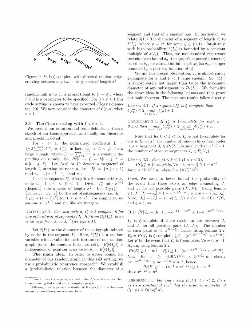
Figure 1: Iux is ξ-complete with directed random edges

crossing between any two subsegments of length xξ

random link is to j, is proportional to |i − j|r, wherer ≥ 0 is a parameter to be specified. For 0 ≤ r ≤ 1 thiscycle setting is known to have expected θ(log n) diame-ter [20]. We now consider the diameter of C(r, n) whenr > 1.

3.1 The C(r, n) setting with 1 < r < 2.We present our notation and basic definitions, then a

sketch of our basic approach, and finally our theoremsand proofs in detail.

For r > 1, the normalized coefficient L =1/(2

∑n/2d=1 d−r) = θ(1); in fact, 1

2Cr< L < 1

Crfor n

large enough, where Cr =∑∞

i=1 i−r is a constant de-pending on r only. So, Pr[i → j] = L|i − j|−r =θ(|i − j|−r). Let Il(u) or Iu

l denote a ‘segment’ oflength l, starting at node u, i.e. Iu

l = u, (u + 1)mod n, . . . , (u + l − 1) mod n.

Consider segment Iux of length x for some arbitrary

node u. Let 0 < ξ < 1. Divide Iux into x1−ξ

(disjoint) subsegments of length xξ. Let Dξ(Iux ) =

J1, J2, . . . , Jx1−ξ be this set of subsegments, i.e. Jk =Ixξ(u + (k − 1)xξ) for 1 ≤ k ≤ xξ. For simplicity, weassume xξ, x1−ξ and the like are integers.

Definition 2. For each node u, Iux is ξ-complete if for

any ordered pair of segments (Ji, Jk) from Dξ(Iux ), there

is an edge from Ji to Jk5(see figure 1).

Let δ(Iux ) be the diameter of the subgraph induced

by nodes in the segment Iux . Here, δ(Iu

x ) is a randomvariable with a value for each instance of our randomgraph (once the random links are set). E[δ(Iu

x )] isindependent of position u, so we let δx = E[δ(Iu

x )].The main idea. In order to upper bound the

diameter of our random graph in this 1-D setting, weuse a probabilistic recurrence approach6. We establisha (probabilistic) relation between the diameter of a

5If we think of a super-graph with the Ji’s as it’s nodes thenthese crossing links make it a complete graph

6Although our approach is similar to Karp’s [13], his theoremsnecessity conditions are not met here.

segment and that of a smaller one. In particular, werelate δ(Ix) (the diameter of a segment of length x) toδ(Iy), where y = xξ for some ξ ∈ (0, 1). Intuitively,with high probability, δ(Ix) is bounded by a constantmultiple of δ(Iy). Thus, we use standard recurrencetechniques to bound δn (the graph’s expected diameter)based on δx0 for a small initial length x0 (so δx0 is upperbounded by a poly-log function of n).

We use this crucial observation: Ix is almost surelyξ-complete for x and ξ < 1 large enough. So, δ(Ix)is almost surely not larger than twice the maximumdiameter of any subsegment in Dξ(Ix). We formalizethe above ideas in the following lemmas and then proveour main theorem. The next two results follow directly.

Lemma 3.1. If a segment Iux is ξ-complete then

δ(Iux ) ≤ 2 max

J∈Dξ(Ix)δ(J) + 1.

Corollary 3.1. If Iux is ξ-complete for each u =

0..n-1 then maxu=0..n−1

δ(Iux ) ≤ 2 max

u=0..n−1δ(Iu

xξ) + 1.

Note that for 0 < ξ < .5, Iux is not ξ-complete for

any u. Since xξ, the number of random links from nodesin a subsegment Ji ∈ Dξ(Ix), is smaller than x1−ξ − 1,the number of other subsegments Jk ∈ Dξ(Ix).

Lemma 3.2. For r/2 < ξ < 1 (1 < r < 2),Pr[Iu

x is ξ-complete, ∀u = 0..n− 1] ≥ 1− n−2

for x ≥ c ln1

2ξ−r n, where c = (10Cr)1

2ξ−r .

Proof. We need to lower bound the probability ofthe event that there exists an edge connecting Ja

and Jb for all possible pairs (Ja, Jb). Using lemma2.1, Pr[Ja → Jb] ≥ 1− e−qε|Ja||Jb|, where ε = ε(Ja, Jb).Note, |Ja| = |Jb| = xξ, ε(Ja, Jb) ≥ Lx−r > .5Lx−r/Cr

and q = 1, so

(3.1) Pr[Ja → Jb] ≥ 1−e−Lx−r×x2ξ ≥ 1−e−.5x2ξ−r/Cr

Ix is ξ-complete if there exists an arc between Ja

and Jb for all possible pairs (Ja, Jb). The numberof such pairs is < x2(1−ξ), hence using lemma 2.2,Px = Pr[Ix is ξ-complete] ≥ 1− (e−.5x2ξ−r/Cr × x2−2ξ).Let E be the event that Iu

x is ξ-complete, ∀u = 0..n−1.Again, using lemma 2.2:Pr[E] ≥ 1− n(1− Px) ≥ 1− (ne−.5x2ξ−r/Cr × x2−2ξ).Now, for x ≥ (10Cr)

12ξ−r × ln

12ξ−r n, clearly

ne−.5x2ξ−r/Cr ≤ ne−5 ln n = n−4, hencePr[E] ≥ 1− (n−4 × x2−2ξ) ≥ 1− n−2

since x2−2ξ < n2.

Theorem 3.1. For any r such that 1 < r < 2, thereexists a constant β such that the expected diameter ofC(r, n) is O(logβ n).

Proof. Since r < 2 we can choose r/2 < ξ < 1. Let φ(x)be a random variable s.t. φ(x) = max

u=0..n−1δ(Iu

x ). φ(x) is

determined for each instance of our random graph. IfIux is ξ-complete for all u = 0..n− 1 then from corollary

3.1, φ(x) ≤ 2φ(xξ) + 1. Thus from lemma 3.2, forx ≥ x0 = (10Cr)

12ξ−r log

12ξ−r n,

(3.2) Pr[φ(x) ≤ 2φ(xξ) + 1] ≥ 1− n−2

We can use a standard recurrence technique toupper bound φ(n), based on φ(x0) and n only.

Define the sequence xit+1i=0, where xi+1 = xb

i withb = 1/ξ, x0 = c log

12ξ−r n, and

t = blogb(logx0n)c = b log( log n

log x0)

log b c = log log nlog b + 0(1)

Thus xt ≤ n < xt+1. Now we look closer atthis sequence φ(xi)t

i=0 and use (3.2) to upper boundthe last term (which differs from φ(n) by a constantmultiple), based on the first term and t. We claim thateach of the events Ei : “φ(xi) ≤ 2φ(xi−1) + 1”, i =1, 2, . . . , t and Et+1 : “φ(n) ≤ 2φ(xt) + 1” occurs withprobability at least 1 − n−2. The first t events can bejustified directly from (3.2), while we can also easilyextend our proof of lemma 3.1 to justify the last event.Let E be the event that E1, E2, . . . , Et+1 all occur.Using lemma 2.2, E occurs with probability at least1− (t + 1)× n−2 ≥ 1−O(n−1).

It is easy to see that event E implies φ(xi) ≤2iφ(x0) + 2i − 1, ∀i = 1..t and thus,φ(n) ≤ 2t+1φ(x0) + 2t+1 − 1 ≤ O((log n)logb 2)× φ(x0).Note that φ(x0) ≤ x0 = (10Cr)

12ξ−r log

12ξ−r n. That is,

Pr[δ(In) ≤ c logβ n)] ≥ 1−O(n−1)where β = log1/ξ 2 + 1

2ξ−r and c depends on r and ξ

only. Thus, Pr[δ(In) ≤ O(logβ n)] tends to 1 when ngoes to infinity, and almost surely δ(In) = O(logβ n).

Note that our bound on β grows rapidly as rapproaches 2.

3.2 The C(r, n) setting with 2 < r

Theorem 3.2. For r > 2, C(r, n) is a ‘large’ world withexpected diameter Ω(n

r−2r−1−o(1)).

Proof. Let 1r−1 < γ < 1. For any node i, the probability

that i’s random contact is at most a distance nγ from i,is 1−O(

∑n/2d=nγ d−r) = 1−O(n−γ(r−1)). Using lemma

2.2, the probability that all random links have length atmost nγ , is ≥ 1−n×O(n−γ(r−1)) = 1−O(n1−γ(r−1)).Since 1

r−1 < γ, this probability tends to 1 when n goesto infinity. Thus the diameter is at least n

nγ = n1−γ withoverwhelming probability (tending to 1 when n goes toinfinity). So, the expected diameter is Ω(n

r−2r−1−o(1))

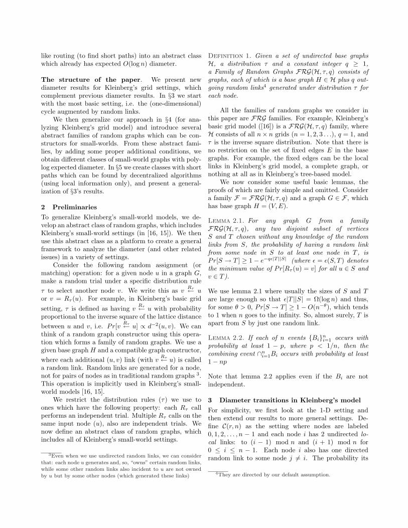
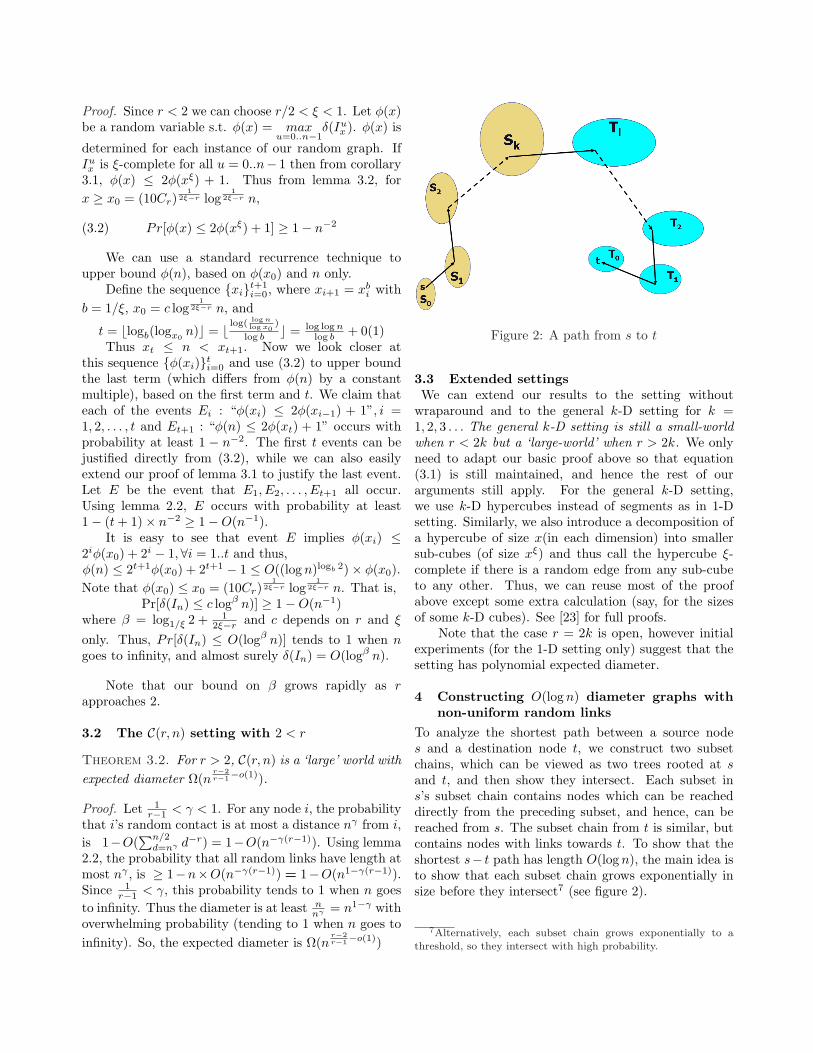
Figure 2: A path from s to t

3.3 Extended settingsWe can extend our results to the setting without

wraparound and to the general k-D setting for k =1, 2, 3 . . . The general k-D setting is still a small-worldwhen r < 2k but a ‘large-world’ when r > 2k. We onlyneed to adapt our basic proof above so that equation(3.1) is still maintained, and hence the rest of ourarguments still apply. For the general k-D setting,we use k-D hypercubes instead of segments as in 1-Dsetting. Similarly, we also introduce a decomposition ofa hypercube of size x(in each dimension) into smallersub-cubes (of size xξ) and thus call the hypercube ξ-complete if there is a random edge from any sub-cubeto any other. Thus, we can reuse most of the proofabove except some extra calculation (say, for the sizesof some k-D cubes). See [23] for full proofs.

Note that the case r = 2k is open, however initialexperiments (for the 1-D setting only) suggest that thesetting has polynomial expected diameter.

4 Constructing O(log n) diameter graphs withnon-uniform random links

To analyze the shortest path between a source nodes and a destination node t, we construct two subsetchains, which can be viewed as two trees rooted at sand t, and then show they intersect. Each subset ins’s subset chain contains nodes which can be reacheddirectly from the preceding subset, and hence, can bereached from s. The subset chain from t is similar, butcontains nodes with links towards t. To show that theshortest s− t path has length O(log n), the main idea isto show that each subset chain grows exponentially insize before they intersect7 (see figure 2).

7Alternatively, each subset chain grows exponentially to athreshold, so they intersect with high probability.

Exponential growth will be likely if each time wegrow a new subset, with high probability more than onelink from each node leaves the current subset. This wastrue in Kleinberg’s grid setting [20] (we called this: “linkinto or out of a ball” property). We now include thisfeature to refine our basic class FRG(H, τ, q). Recallthat, a family of random graphs FRG(H, τ, q) consistsof graphs, each of which is a base graph H ∈ Hplus at least q out-going random links generated underdistribution τ for each node.

Definition 3. For constants µ > 0 and ξ > 0, familyF = FRG(H, τ, q) meets ‘the (µ,ξ) expansion criterion’,or F is (µ,ξ)-EXP , if ∀H = (V,E) ∈ H, with n = |V |:

(4.3) ∀u ∈ V, ∀C ⊂ V, |C| < nµ : Pr[v Rτ← u : v /∈ C] ≥ ξ

For example, from [19], it is easy to verify thatKleinberg’s grid setting with wrap-around distance is(µ,1 − µ − o(1))-EXP for any fixed positive constantµ < 1. This criterion supports diversity and fairnessin the distribution of random links: For a random linkfrom any node, no small set of vertices (size ≤ nµ) cantake most of the chance to have this link come into it.

Definition 4. (Type µ-Expansion) For a constantµ > 0, type µ-Expansion contains all the familiesFRG(H, τ, q) which meet (µ,ξ)-EXP for some ξ > 1/q.

We define χ, called an ‘expansion function’, asfollows. Given any u ∈ V , this operation will calloperation Rτ q times. Also, let χ(u) denote the set ofvertices from these q Rτ calls. Thus the random linksfor graph G are formed by performing operation χ oneach node. For any set S: χ(S) =

⋃u∈S χ(u).

Consider a family F of type µ-Expansion. Letβ = qξ (so β > 1). For any node u and set C of sizeless than nµ − q, which is determined before χ(u) isknown, the expected number of fresh elements generatedby χ(u) that do not belong to C is greater than β:E[ | χ(u)− C | ] > β > 1. Since χ(u) ‘contributes’ morethan one expected fresh element outside of C, χ can beused to generate a chain of subsets from a small initialsubset such that with high probability, the subsets willquickly grow to size Θ(nµ).

4.1 The out-going subset chain Let F be a µ-Expansion family, and G = (V, E) be an arbitrarygraph from F . Now, from an arbitrary initial setS0 ⊂ V , we construct a chain of subsets Sk, namelythe out-going subset chain with respect to the initial setS0, s.t. Sk+1 = χ(Sk)−∪k

i=0Si; k = 1, 2, 3, . . . Thus, Si

is the nodes at distance i from S0 using random links.The following results for µ-Expansion families show thesubset chain grows rapidly if S0 is large enough.

Lemma 4.1. ∀C, S ⊂ V s.t. S ⊂ C, |C| ≤ α = θ(nµ): if|S| = Ω(log n), almost surely |χ(S) − C|/|S| > γ for aconstant γ > 1. Also, ∃γ > 1, ∀ θ > 0,∃c > 0:

|S| > c log n ⇒ Pr[ |χ(S)−C||S| > γ] = 1−O(n−θ)

The above lemma (see [23] for proof) provides aprobabilistic lower bound γ on the growth rate of thesubset chain in each early step (by choosing C = ∪k

i=0Si

to apply the lemma in each step). This growth rate canbe maintained as long as the subset sizes are still undera threshold. For any S0 ∈ V with size Ω(log n), thesubset chain originating from S0 will almost surely growexponentially in size until it reaches size α = θ(nµ).Also, for any θ > 0, by choosing a sufficiently largeconstant c s.t. |S0| > c log n, Pr[|Sk| ≥ α] = 1−O(n−θ)for some k = O(log n). Moreover, this can be true forany given θ > 0 by choosing c large enough.

4.2 The in-coming subset chain We now con-struct a subset chain, based on the random links comingto the sets of the chain. We use an ‘expansion function’ψ, which is a counterpart of χ, so we can reuse theformalism used in §4.1 on the out-going subset chainand obtain similar results. Function ψ is not state-lessas χ was. For any subset of vertices D and a nodeu ∈ V we define ψ(u,D) to return the set of all nodesv /∈ D s.t. v has a random link to u. As before,ψ(T,D) =

⋃u∈T ψ(u,D) for any subset T . Now, from

an arbitrary subset T0 ⊂ V , we can construct a chain ofsubsets Tk, namely the in-coming subset chain withrespect to the initial set T0, s.t. Tk+1 = ψ(Tk,D) fork = 1, 2, 3, . . ., where D = ∪k

i=0Tk. Similar to definition3, we have:

Definition 5. For constants µ > 0 and ξ > 0, familyF meets ‘the (µ,ξ) incoming expansion criterion’, or Fis (µ,ξ)-IE, if the following is satisfied.

(4.4) ∀D : |D| < nµ, ∀u ∈ D : Pr[∃v /∈ D : Rτ (v) = u] > ξ

Similarly as with µ-Expansion, for a fixed µ > 0,we define type µ-IncExpansion, which includes allthe FRG(H, τ, q) families which meet (µ,ξ)-IE whereξ > 1/q. For a µ-IncExpansion family, lemma 4.1holds if we replace the use of function χ by that offunction ψ and subset C by subset D (8). There isan interesting implication between these two expansioncriteria for a large class of families. We call a familyof random graphs, using a distribution τ , δ-symmetric(or just symmetric if δ = 1) for some constant δ ≥ 1, ifPr[Rτ (v)=u]Pr[Rτ (u)=v] ≤ δ for all pairs of nodes (u, v). It is easy

8The constructions of both subset chains share the sameformalism

to see that Kleinberg’s grid settings (using the inversepower distributions) have this property, and they aresymmetric if wrap-around distance is used.

Lemma 4.2. If family F is (µ,ξ)-EXP , for 0 < µ, ξ <1, and is δ-symmetric for some δ ≥ 1 then F is(µ,1− e−ξ/δ)-IE.

Proof. [Proof(sketch)] We need to prove (4.4) holds.Let p(u, v) = Pr[Rτ (u) = v] and F be the eventthat ∃v /∈ D : Rτ (v) = u. The lemma is shownas Pr[F ] =

∏v/∈D(1 − p(v, u)) ≤ ∏

v/∈D e−p(v,u) =exp−∑

v/∈D p(v, u) ≤ exp− 1δ

∑v/∈D p(u, v) ≤ e−

ξδ .

Note that∑

v/∈D p(u, v) = Pr[∃v /∈ D : Rτ (u) = v] ≥ ξ.

4.3 Abstract classes of small-world graphs Werefine the above families by adding conditions to obtainsmall-world graphs. If our graph is from a familyof type µ1-Expansion and µ2-IncExpansion for some0 < µ1, µ2 < 1 then, given any source s and destinationt, we can use the following strategy to construct a log n-length path from s to t (see figure 2). First, we want aconnected subset S0 containing s and T0 containing t ofΩ(log n) size in the base graph H. We then constructthe out-going subset chain from S0 and the in-comingsubset chain from T0. Our above results show that,with overwhelming probability, there exist subsets Sk

with size θ(nµ1) and Tl with size θ(nµ2) s.t. any nodein Sk can be reached from S0 by O(log n) links, andT0 from Tl by O(log n) links. We now consider properconditions so we can easily reach Tl from Sk.

If ε = ε(τ), the minimum value of Pr[Rτ (u) = v]for all u 6= v, is large enough, then almost surely thereis an arc from Sk to Tl (or they intersect).

Definition 6. (Expansion Family) A FRG(H, τ, q)is an Expansion family if it is (µ1,ξ)-EXP and(µ2,ξ)-IE for some constants ξ > 1/q, µ1, µ2 > 0, andε(τ) = Ω(n−µ3) for a constant µ3 < µ1 + µ2.

We now show that a graph from an Expansionfamily almost always has an arc from Sk to Tl (or theyalready intersected). We can assume all the nodes in Sk

are fresh (we do not know their random links yet9) andhence, using lemma 2.1, Pr[Sk → Tl] ≥ 1−e−qε|Tl||Sk| ≥1−e−Ω(nµ1+µ2−µ3 ) ≥ 1−O(n−1), which tends to 1 whenn goes to the infinity.

9We omit a conditioning issue: if we construct the s subsetchain (s-SSC) first then the growth of the t subset chain (t-SSC)is conditioned on the existence of s-SSC and vice versa. Thus, weneed to add ∪k−1

i=0 Si to D (§4.2) or ∪l−1i=0Ti to C (4.1). Therefore,

if µ1 > µ2 then we construct t-SSC first, otherwise s-SSC first.

The graphs from an Expansion family 10 aresmall-worlds, i.e. their expected diameter is poly-login n, as long as each node is rich enough in neighbors inthe base graph to form large enough initial subsets (i.e.S0, T0). Without this final condition, however, oftenthese graphs are not connected. If there are no edges inthe base graph (E = ∅) then even with the added ran-dom edges, the graphs can be unconnected; an examplewill be presented in the next subsection.

We now add the notion of neighboring in thebase graphs. A node u is called k-neighbored forsome k ∈ N if u belongs to a connected componentof size k in the base graph. A base graph H =(V, E) is called k-neighbored if all the nodes are k-neighbored. A connected graph is k-neighbored for allk ≤ |V | − 1. For k large enough, k-neighbored graphsallow us to construct large enough initial subsets. Thenext theorem now follows fairly directly11.

Theorem 4.1. For any two nodes s, t in a graph of anExpansion family , if s and t are c log n-neighboredfor any constant c > 0 then there almost surely existO(log n)-length paths between s and t. An Expansionfamily , using (c log n)-neighbored base graphs wherec > 6qξ

(qξ−1)2 , has expected diameter O(log n).

Thus, a graph from an Expansion family almostalways consists of a giant component with diameterO(log n) and perhaps some small components of sizeO(logn). There are perhaps random (directed) linksbetween the components (but only in one directionbetween a given pair).

Using super-nodes. We now consider randomgraphs which use log n-neighbored base graphs.

Theorem 4.2. Consider a family FRG(H, τ, q), whichis (µ1,ξ)-EXP and (µ2,ξ)-IE for some constantsξ, µ1, µ2 > 0, where ε(τ) = Ω(n−µ3) for some con-stant µ3 < µ1 + µ2, and all base graphs in H are log n-neighbored. There almost surely exists a path of lengthO(log n) between any two nodes (for n large enough).

Proof. This theorem is a simple corollary of the previoustheorem if q is s.t. ξ > 1/q. However, for q < Q = d1/ξethe theorem still holds. The main idea is to formsuper-nodes with Q random links. The log n-neighboredproperty assures that we can always partition the graphinto super-nodes each of which is a subgraph of constantdiameter and has at least Q random links. The lengthof a path constructed here differs by only a constantfrom before (when we have q ≥ Q).

10Note that we can construct similar classes by using µ-Expansion and δ-symmetric property instead.

11In fact, a full proof of it is very similar to that of theorem 14in our previous work [20].

Figure 3: The hierarchy of classes

These abstract classes for (almost) small-worldgraphs are broad enough to accommodate many dif-ferent well-known small-world models: Bollobas andChung’s [6], Watts and Strogatz’s [24], Kleinberg’s grid-based [16], tree-based, and group-induced models [15].Kleinberg describes his group-induced model with twoabstract properties, and it is not hard to see that the sec-ond property implies our (µ,ξ)-IE for some 0 < µ, ξ < 1.We show that our results apply to Kleinberg’s tree-basedmodel in the following section. It is relatively straight-forward to extend this case for similar results in thegroup-induced model. Figure 3 shows how the classesrelate.

4.4 The diameter of a tree-based random graphWe now use our framework to analyze the diameterof Kleinberg’s tree-based model [15] and its variants.Kleinberg shows that decentralized routing can be ap-plied in more settings (not only the grid-based [16]),but even when no lattice structure appears at all (say,the network of the Web’s hyper-links). Kleinberg alsointroduces a group-induced model, a generalization ofboth grid-based and tree-based models [15]. He showsthat using these models, greedy routing takes expectedtime O(log n) if nodes have out-degree θ(log2 n), andO(log4 n) if the degrees are bounded by a constant.

In Kleinberg’s tree-based model nodes are the leavesof a complete (for simplicity) b-ary tree T , where b isa constant. Let h(u, v) denote the height of the leastcommon ancestor of u and v in T . There are no local

links in this setting but there are a number of directedrandom links leaving each node u, under a distributionτ , where a link is to v with probability proportional tob−h(u,v).

If there are exactly q directed random links leavingeach node, the graphs in this tree-based setting arevery likely unconnected (similar to the case of lackinglocal links in the grid-based setting [19]), however, thesetting can still be an Expansion family by addingproper conditions. From [15], the normalizing coefficientof this link distribution is θ(log−1 n). So, ε(τ) =θ(n−1 log−1 n); thus, to have an Expansion family weneed this setting to meet (µ1,ξ)-EXP and (µ2,ξ)-IE forsome ξ > 1/q and µ1 + µ2 > 1. Consider the followingfact which holds even if q = 1.

Fact 4.1. For Kleinberg’s tree graphs with any q ≥ 1,given a positive θ < 1, a node u and C ⊂ V with size atmost nθ, the probability that a random link from u hits anode outside of C is more than 1−θ−o(1) when n is largeenough. Also, the probability that there is a random linkto u from outside of C is more than 1 − eθ+o(1)−1 (i.e.almost 1− eθ−1) when n is large enough.

See [20] for a proof of a similar fact. It is easy tosee that the setting meets (x − o(1),1 − x)-EXP and(y − o(1),1− ey−1)-IE for any 0 < x, y < 1. Therefore,given q, we need to find x, y s.t.

x + y > 1; q(1− x) > 1; q(1− ey−1) > 1Solving this system of equations, we find q ≥ 3.

Theorem 4.3. For q ≥ 3, Kleinberg’s tree-based set-ting is an Expansion family .

We can add in local links to make the base graphconnected or make the base graph c log n-neighbored:ring all the nodes in the base graph H or alternately,ring all the subtrees of height at most logb(c log n). Withc determined as in theorem 4.1, this setting will haveexpected diameter O(log n).

5 Random graphs induced by semi-metric ormetric functions

We have abstracted away topological features of Klein-berg’s grid setting with our expansion criteria to createclasses where the strongest has O(log n) expected diam-eter. We now generalize the use of a distance measure inthe distribution of random links, and this makes greedy-like routing (defined later) work. We design classes ofrandom graphs using distributions based on semi-metricfunctions: we define a semi-metric function d(u, v) andgenerate random links between any two nodes u and vwith probability ∝ d−r(u, v). We omit proofs in thissection, which can be found in [23].

Consider a pair (G, d): a graph G = (V, E) anda function d = dG : V 2 → R+ associated with G.We define d to be a semi-metric function if for anyu, v ∈ V , d(u, v) = 0 ⇔ u = v; and d(u, v) = d(v, u).We define Nk(u) = v ∈ V |d(u, v) ≤ k, the nodeswithin ‘distance’ k of u. For c1, c2 > 0, graph Gis called (c1, c2) linear-expanded with respect to d if∀u ∈ V, k = 1, 2 . . . : c1 ≤ |Nk(u)|

k ≤ c2 if Nk−1(u) 6= V ,i.e. |Nk(u)| grows nearly-proportionally to k beforeNk(u) becomes V .

Definition 7. (InvDist family) An InvDist(r) is aFRG(H, τ, q) family where each base graph H ∈ Hhas an associated metric-function d and there existsconstants c1, c2 > 0 s.t. H is (c1, c2) linear-expandedw.r.t d, and where 12: Pr[Rτ (u) = v] ∝ d−r(u, v).

All Kleinberg’s small-world models (grid-based,tree-based and group-induced) fall into InvDist(1) foran appropriate d. For example, for Kleinberg’s 2-D gridmodel [16], we define d(u, v) as the square of the latticedistance between u and v; for Kleinberg’s group-inducedmodel [15], we define d(u, v) as the size of the minimumset containing both u and v 13.

Theorem 5.1. ∀r : 0 < r < 1, δ > 0, c2 > c1 > 0,∃q ≥ 1 s.t. any δ-symmetric InvDist(r) family specifiedby c1, c2 and q (as in definition 7) is an Expansionfamily .

For any graph from a δ-symmetric InvDist(r) fam-ily using log n-neighbored base graphs, there almostsurely exists an O(log n) length path between any twonodes14.

5.1 Greedy-like routing.This section constructs a new class of graphs where

most pairs of nodes have shortest paths of lengthO(log n) and greedy-like paths (defined below) withexpected length O(log2 n). Inspired by Kleinberg’s ideaof greedy routing using only local information [16], weassume that each node u knows the random links whichleave nodes in a small neighborhood near u (e.g. thelog n nodes closest to u in the base graph). Greedy-likepaths are paths found by a greedy-like algorithm whichis defined as follows: if the current node is u, choose the

12Note that any family satisfying all these criteria except having

c1 ≤ |Nk(u)|kβ ≤ c2 instead (for some given constant β > 0) can

be normalized by using function d′(u, v) = dβ(u, v) instead, andhence becomes an InvDist(r′) family where r′ = r/β.

13It is not hard to see that the second property (of the twoabstract properties Kleinberg uses to describe his group-inducedmodel) implies that |Nk(u)| grows nearly-proportionally to k.

14Note that if we only use undirected random links then thecondition of δ-symmetry is not necessary.

random link (w, v) where w is in u′s neighborhood andv is the closest such node to the destination. Route tow using local links and then take link (w, v). Update vto be the current node. We now present new definitionsand then our theorems for this routing strategy.

We restrict d(u, v) to be a ‘light’ metric by addingthe condition that d(u, v) ≤ α(d(u,w)+d(w, v)) for anynodes u, v, w and for a constant α (so less strict than thetriangle inequality). We define class MET R(r) as classInvDist(r) but each function d is a light metric functioninstead. All Kleinberg’s small-world models (grid-based,tree-based and group-induced) are MET R(1) familieswith the function d(u, v) derived naturally from eachmodel’s context. Except for the 1-D and the tree-basedsetting, this function is not a metric. For the tree-based setting, let d(u, v) be the number of leaves in thesmallest subtree containing u and v (this satisfies thetriangle inequality). For the group-induced model, welet d(u, v) be the size of the smallest group containingnodes u and v. This generally doesn’t satisfy thetriangle inequality, but satisfies ours for a proper α.

We now add neighboring conditions so our greedy-like routing strategy can be used. An undirected basegraph H(V,E) is called k-strongly neighbored if for eachu ∈ V , the sub-graph induced by the set of nodes v suchthat d(u, v) ≤ k is connected.

Theorem 5.2. For any graph from a MET R(1) familyusing log n-strongly neighbored base graphs, a greedy-likealgorithm will find paths of expected length O(log2 n)between any two nodes.

Combining theorems 5.1 and 5.2, we have:

Theorem 5.3. For any graph from a MET R(1) δ-symmetric family using log n-strongly neighbored basegraphs, there almost surely exists a path of lengthO(log n) and a greedy-like path of expected O(log2 n) be-tween any two nodes.

This theorem easily applies to Kleinberg’s grid,tree-based and group-induced models with proper lo-cal links (to make the base graphs log n-strongly neigh-bored).

5.2 Diameter of MET R(r) for 1 < r < 2.

We now present a natural generalization of our resultsin §3. We consider the diameter of MET R(r), where1 < r < 2.

Theorem 5.4. For 1 < r < 2, for a MET R(r) family,there exists a constant c s.t. if the base graphs are x0-strongly neighbored, where x0 = c log

22−r n (n: number

of vertices), then almost surely the expected diameter ofthis family is upper bounded by a poly-log function.

For example, we can modify Kleinberg’s tree-basedsetting to become a small-world graph with poly-logexpected diameter as follows. We connect all the nodestogether (say, order the nodes from left to right andconnect them with undirected edges), and for any twonodes u and v, we add an arc from u to v withprobability proportional to b−rh(u,v) instead of b−h(u,v)

with 1 < r < 2. Note that, under the context of thissection we define d(u, v) as the number of leaves in thesmallest subtree 15 which contains both u and v: bh(u,v).

6 Concluding remarks

We consider a general construction of random graphs:a base graph plus random links added to each node. Bygradually adding properties to the base graphs and/orthe distribution of random links, we build a hierarchy ofclasses of random graphs with the finest ones featuringsmall-world properties (small diameter and greedy-likerouting using local information only). Thus, we proposea framework for analyzing and characterizing small-world graphs.

There are still some open questions in our study of‘adding links with probability ∝ the inverse distance’.As noted before, the case r = 2k in the k-D grid settingis still open. We also expect to extend our resultsin §5 for base graphs with restricted growth rate16, ageneral class of graphs which can be used to model manyreal networks [12]. Thus our work can be useful for apractical design problem, where we want to add in “longlinks” to a given network to shrink its diameter.

References

[1] J. Aspnes, Z. Diamadi, G. Shah, “ Fault-tolerantRouting in Peer-to-peer Systems”, Proc. 22nd ACMSymp. on Princ. of Dist. Comp., PODC’02, p. 223-232

[2] L. Barriere, P. Fraigniaud, E. Kranakis, D. Krizanc,“Efficient Routing in Networks with Long Range Con-tacts”, Proc. 15th Intr. Symp. on Dist. Comp., DISC’01,p. 270-284

[3] I. Benjamini and N. Berger, “The Diameter of a Long-Range Percolation Clusters on Finite Cycles” RandomStructures and Algorithms, 19,2:102-111 (2001).

[4] M. Biskup, “Graph Diameter in Long-range percola-tion”, submitted to Electron. Comm. Probab.

[5] B. Bollobas, “The Diameter of Random Graphs”, IEEETrans. Inform. Theory 36 (1990), no. 2, 285-8.

[6] B. Bollobas, F.R.K. Chung, “The diameter of a cycleplus a random matching”, SIAM J. Discrete Math.1,328-333 (1988)

15Or we can use the size of the subtree: ≈ bb−1

bh(u,v)

16Where, informally, any ‘ball’ with radius r around a node uhas at most O(rβ) nodes for some fixed constant β > 0.

[7] F. Chung and L. Lu, “The Diameter of Random SparseGraphs”, Adva. in App. Math. 26 (2001), 257-279.

[8] D. Coppersmith, D. Gamarnik, and M. Sviridenko “Thediameter of a long- range percolation graph”, RandomStructures and Algorithms, 21,1:1-13 (2002).

[9] P. Dodds, R. Muhamad, and D. Watts, “An experimen-tal study of search in global social networks”, Science,301:827-9, 2003.

[10] P. Erdos and A. Renyi, “On random graphs”, Publica-tiones Mathematicas 6, 290-7 (1959).

[11] P. Fraigniaud, C. Gavoille and Christophe Paul, ”Eclec-ticism Shrinks the World”, Proc. 23rd ACM Symp. onPrinc. of Dist. Comp. PODC’04, p. 169-178.

[12] J. Gao and L. Zhang, “Tradeoffs between StretchFactor and Load Balancing Ratio in Routing on GrowthRestrict Graphs”, Proc. 23rd ACM Symp. on Princ. ofDist. Comp. PODC’04, p. 189-196.

[13] R. Karp, “Probabilistic Recurrence Relations”, in Jour-nal of the ACM 41(6):1136-1150, Nov. 1994.

[14] D. Kemper, J. Kleinberg, and A. Demers, “Spatialgossip and resource location protocols”, in Proc. ACMSymp. Theory of Computing, 163-172, 2001.

[15] J. Kleinberg, “Small-World Phenomena and the Dy-namics of Information”, in Advances in Neural Infor-mation Processing Systems (NIPS) 14, 2001.

[16] J. Kleinberg, “The Small-World Phenomenon: AnAlgorithmic Perspective”, in Proc. 32nd ACM Symp.Theory of Comp., 163-170, 2000.

[17] M. Kochen, Ed., The Small-World (Ablex, Norwood,1989)

[18] G. S. Manku and M. Naor and U. Wieder, “KnowThy Neighbour’s Neighbour: The Role of Lookahead inRandomized P2P Networks”, Proc. 36th ACM Symp.on Theory of Comp. STOC’04, p. 54-63.

[19] C. Martel and V. Nguyen, “The complexity of mes-sage delivery in Kleinberg’s Small-world Model”, Tech-Report CSE-2003-23, CS-UCDavis, 2003.

[20] C. Martel and V. Nguyen, “Analyzing Kleinberg’s (andother) Smallworld Models”, Proc. 23rd ACM Symp. onPrinc. of Dist. Comp. PODC’04, pp. 179-188.

[21] D. Malkhi, M. Naor, D. Ratajczak, “Viceroy: A Scal-able and Dynamic Emulation of the Butterfly”, Proc.21st ACM Symp. on Princ. of Dist. Comp., p. 183-192.

[22] S. Milgram, “The small world problem” PsychologyToday 1,61 (1967).

[23] V. Nguyen and C. Martel, “Analysis and Models forSmall-World Graphs”, Tech-Report CS-UCDavis, 2004.www.cs.ucdavis.edu/˜martel/main/smallworld.tech.pdf

[24] D. Watts and S. Strogatz, “Collective Dynamics ofsmall-world networks” Nature 393,p. 440-2 (1998).

[25] H. Zhang, A. Goel and R. Gividan, “Using the Small-World Model to Improve Freenet Performance”, IEEEINFOCOM’02, vol. 21(1), pp. 1228-37.