Florida International UniversityFIU Digital Commons

FIU Electronic Theses and Dissertations University Graduate School

11-13-2015

Cobalt Ferrite Nanoparticles Fabricated via Co-precipitation in Air: Overview of Size Control andMagnetic PropertiesDennis ToledoFlorida International University, dtole007@fiu.edu

DOI: 10.25148/etd.FIDC000195Follow this and additional works at: https://digitalcommons.fiu.edu/etd

Part of the Bioimaging and Biomedical Optics Commons, Biomaterials Commons, BiomedicalCommons, Ceramic Materials Commons, Nanotechnology Fabrication Commons, and the OtherBiomedical Engineering and Bioengineering Commons

This work is brought to you for free and open access by the University Graduate School at FIU Digital Commons. It has been accepted for inclusion inFIU Electronic Theses and Dissertations by an authorized administrator of FIU Digital Commons. For more information, please contact dcc@fiu.edu.

Recommended CitationToledo, Dennis, "Cobalt Ferrite Nanoparticles Fabricated via Co-precipitation in Air: Overview of Size Control and MagneticProperties" (2015). FIU Electronic Theses and Dissertations. 2298.https://digitalcommons.fiu.edu/etd/2298

FLORIDA INTERNATIONAL UNIVERSITY

Miami, Florida

COBALT FERRITE NANOPARTICLES FABRICATED VIA CO-PRECIPITATION IN AIR:

OVERVIEW OF SIZE CONTROL AND MAGNETIC PROPERTIES

A thesis submitted in partial fulfillment of the

requirements for the degree of

MASTER OF SCIENCE

in

BIOMEDICAL ENGINEERING

by

Dennis Toledo

2015

ii

To: Interim Dean Ranu Jung College of Engineering and Computing This thesis, written by Dennis Toledo, and entitled Cobalt Ferrite Nanoparticles Fabricated via Co-precipitation in Air: Overview of Size Control and Magnetic Properties, having been approved in respect to style and intellectual content, is referred to you for judgment. We have read this thesis and recommend that it be approved.

_________________________________ Shuliang Jiao

_________________________________ Jean H. Andrian

_________________________________

Sakhrat Khizroev, Major Professor

Date of Defense: November 13, 2015 The thesis of Dennis Toledo is approved.

_________________________________ Interim Dean Ranu Jung

College of Engineering and Computing

_________________________________ Dean Lakshmi N. Reddi

University Graduate School

Florida International University, 2015

iii

ACKNOWLEDGMENTS

I want to thank my family for their consistent and important support throughout

my Master’s program. I also want to thank all my professors, classmates, and colleagues

for their helpfulness, and for the things which I learned from them. I want to thank my

major professor, Dr. Sakhrat Khizroev, for his assistance and support for the last two

years. Also, I want to thank my other two committee members, Dr. Shuliang Jiao and Dr.

Jean Andrian, for their assistance and support. I want to thank Dr. Rakesh Guduru, for

his support and helpful advice. I want to thank Ali Hadjikhani for imaging my SEM

samples, Emmanuel Stimphil for doing AFM/MFM imaging for me, and Dr. Charles

Packianathan for analyzing my DLS samples. Also, I am grateful to Dr. Barry Rosen for

allowing me to work with Dr. Packianathan in analyzing my DLS samples.

iv

ABSTRACT OF THE THESIS

COBALT FERRITE NANOPARTICLES FABRICATED VIA CO-PRECIPITATION IN AIR:

OVERVIEW OF SIZE CONTROL AND MAGNETIC PROPERTIES

by

Dennis Toledo

Florida International University, 2015

Miami, Florida

Professor Sakhrat Khizroev, Major Professor

Cobalt Ferrite has important, size-dependent magnetic properties. Consequently,

an overview of particle size is important. Co-precipitation in air was the fabrication

method used because it is comparatively simple and safe. The effects of three different

reaction times including 1, 2, 3 hour(s) on particle size were compared. Also, the

effectiveness of three different capping agents (Oleic Acid, Polyvinylpyrollidone (PVP),

and Trisodium Citrate) in reducing aggregation and correspondingly particle size were

examined. Using Welch’s analysis of variance (ANOVA) and the relevant post hoc tests,

there was no significant difference (p=0.05) between reaction times of 1 hour and 2

hours, but there was a significant difference between reaction times of 2 hours and 3

hours. Potentially, because of increased coarsening for the 3 hour reaction time. PVP

and Oleic Acid were shown to be effective in reducing aggregation; however, Citrate was

not effective. Possibly, the synthesis procedure was inadequate.

v

TABLE OF CONTENTS

CHAPTER PAGE Statement of Problem 1 Introduction 1 Chemical Composition and Magnetism 2 Synthesis Procedure 9 Hypotheses 12 Results 13

DLS Data 13 AFM Data 16 SEM Data 24

Discussion 32 Applications 35 Processes and Tools 40

Measurement Tools 40 Materials 43 Methods 43

References 48

vi

LIST OF FIGURES

FIGURE PAGE Figure 1: A Macro view of the fcc CoFe2O4 unit cell. 3 The red dots are lattice points. 3 of the total 6 face lattice points, and 7 of the total 8 corner lattice points are visible. Figure 2: A view of the inside of the fcc CoFe2O4 unit cell. 4 The blue dots are O2- ions. Figure 3: An illustration of forms of magnetism. Based on information from [35]. 6 Figure 4: Illustration of Hysteresis. Based on information from [35] and [76]. 7 Figure 5: A MFM image of PVP 16 Figure 6: An AFM image of PVP 17 Figure 7: Different AFM Image of PVP 17 Figure 8: Different MFM Image of PVP 18 Figure 9: AFM image of CL. Notice the high amount of aggregation. 19 Figure 10: An MFM image of CL 19 Figure 11: AFM image for No OA 20 Figure 12: MFM image for No OA 20 Figure 13: OA On the Left, AFM Image; On the Right, MFM Image. 21 Dipoles (seen as dark to light or vice versa) are clearly visible in the MFM image.

vii

Figure 14: Closer View of AFM image for OA 21 Figure 15: Closer View of MFM image for OA 22 Figure 16: Another AFM image for OA 22 Figure 17: Another MFM image for OA 23 Figure 18: A View of PVP 721 24 Figure 19: A Different View of PVP 721 24 Figure 20: PVP 721 at closer magnification 25 Figure 21: A View of Oleic 721 25 Figure 22: Oleic 721 at closer magnification 26 Figure 23: An image of PVP 723 26 Figure 24: SEM image of PVP 27 Figure 25: An image of PVP at closer magnification 27 Figure 26: SEM image of CL 28 Figure 27: SEM image of CL at closer magnification 28 Figure 28: SEM image of 1hr sample 29 Figure 29: SEM image of Control1 29 Figure 30: SEM image of the sample labeled Oleic 30

viii

Figure 31: SEM image of Hrxn 30 Figure 32: SEM image of sample labeled Citrate 31 Figure 33: SEM image of Procedure Based on [7] 31

1

Statement of Problem

The problem addressed by this work is the fabrication of Cobalt Ferrite

(CoFe2O4) nanoparticles via co-precipitation in air. This fabrication method was chosen

because it is comparatively simple and safe. More specifically, it does not require the

construction of an apparatus to establish a unique atmosphere (such as a nitrogen

atmosphere or an argon atmosphere) for the reaction because the reaction takes place

in air, and the reactants are of low volatility and are less toxic than other potential

reactants (such as n-octane or n-butanol which are sometimes used to fabricate these

particles via microemulsions) [35, 42]. This thesis examines how reaction time and

choice of capping agent affect the size of these nanoparticles. Additionally, this work

discusses other factors which may affect the size of Cobalt Ferrite nanoparticles,

including reaction temperature, stir rate, pH, and ionic strength. Lastly, the magnetic

properties will be examined through magnetic force microscopy (MFM) imaging.

Introduction

Nanotechnology typically involves materials at a length scale of less than 100 nm

[1, 2]. Similarly, nanoparticles are particles at a length scale of less than 100 nm.

Magnetic anisotropy alludes to the fact that what is called the anisotropy energy of a

magnetic material depends on the direction of the spontaneous magnetization vector

[28]. In other words, the magnetization of an anisotropic magnetic material depends on

direction, and certain directions magnetize more easily.

Cobalt Ferrite (CoFe2O4) is characterized by excellent chemical stability, good

mechanical hardness, and useful magnetic properties, including high magnetic

anisotropy, moderate saturation magnetization, high magnetostriction, and high

coercivity [3-6, 29, 32]. The high magnetic anisotropy of Cobalt Ferrite contributes to its

high coercivity, and, owing to this, historically; cobalt oxide modified maghemite

2

nanoparticles were utilized in magnetic recording devices such as audio or video tapes

[49]. Cobalt Ferrite nanoparticles are still harnessed for magnetic recording, but, today,

the applications of these particles also include use as drug delivery systems, magnetic

hyperthermia, and as MRI contrast agents [50, 59, 74, 78]. These will be described later.

Chemical Composition and Magnetism

Transition metal iron oxides have the general formula MFe2O4 where M is a

divalent transition metal or a mixture of transition metal ions [3, 25]. In the case of Cobalt

Ferrite, the transition metal is Cobalt and as such its chemical formula is CoFe2O4. More

specifically, Cobalt Ferrite is a ceramic with an inverse spinel structure [25]. The spinel

structure derives its name from MgAl2O4, which is itself called Spinel, and as such

molecules of the spinel structure possess the general formula AB2O4 [25]. Molecules of

this type are made up of a crystal lattice, which is itself divided into face centered cubic

(fcc) unit cells [25]. A particular unit cell possesses a certain number of lattice points

[33]. Regarding lattice points, there are interior lattice points (Ni) which belong entirely to

one unit cell, face lattice points which belong to two unit cells (Nf), and corner lattice

points (Nc) which belong to eight unit cells [33]. This gives rise to the following formula

for the number of lattice points in a particular unit cell (N) [33].

𝑁𝑁 = 𝑁𝑁𝑖𝑖 +𝑁𝑁𝑓𝑓2

+𝑁𝑁𝑐𝑐8

Given that an fcc unit cell does not have any interior lattice points (Ni), but does

have six face lattice points (Nf), and eight corner lattice points (Nc) the total number of

lattice points (N) per fcc unit cell is four [25, 33]. Each fcc unit cell is composed of fifty-six

ions, and therefore there are fourteen ions associated with each lattice point [25].

Fcc unit cells are stabilized by tetrahedral interstitial sites and octahedral

interstitial sites, and, for the spinel structure, each fcc unit cell has twice as many

3

available tetrahedral sites (sixty-four sites) as available octahedral sites (thirty-two sites)

[25, 31, 33-34]. In spite of this difference in available sites, owing to the fact that each fcc

unit cell is made up of only fifty-six ions, specifically thirty-two oxygen anions, eight “A”

cations, and sixteen “B” cations, in which “A” and “B” refer to the general spinel structure

(AB2O4), clearly not all available interstitial sites are occupied in each fcc unit cell [25,

31, 34]. In fact twice as many octahedral sites as tetrahedral sites are actually occupied

in each fcc unit cell [31, 34-35]. More precisely, in a normal spinel eight of the tetrahedral

sites are occupied by “A” cations and sixteen of the octahedral sites are occupied by “B”

cations whereas in an inverse spinel structure only eight of the octahedral sites are

occupied by “B” cations, eight other octahedral sites are occupied by “A” cations, and

eight tetrahedral sites are occupied by the other half of the available “B” cations [25, 31,

34-35].

Figure 1 below was created with the help of information in [33]. It shows a view of

the fcc unit cell from the outside.

Figure 1: A Macro view of the fcc CoFe2O4 unit cell. The red dots are lattice points. 3 of

the total 6 face lattice points, and 7 of the total 8 corner lattice points are visible.

4

Figure 2: A view of the inside of the fcc CoFe2O4 unit cell. The blue dots are O2- ions.

Figure 2 above depicts a view of the fcc unit cell from the inside. The occupied

tetrahedral and the occupied octahedral sites shown in Figure 2 repeat in a similar way,

as the way shown, to fill out the unit cell. Recall that there are eight occupied tetrahedral

sites and sixteen occupied octahedral sites [25, 31, 34-35].

In practice, the spinel structure is more complex because molecules do not

always correspond fully to a normal or an inverse structure. Hence, an inversion

parameter, i, defined by 0 < i < 1 is introduced [31]. For CoFe2O4, i ranges from 0.68 to

0.8 meaning that between 68% and 80% of Co2+ ions occupy octahedral sites rather

than 100% of Co2+ ions occupying octahedral sites, which is the case for a fully inverse

spinel structure, described above [31, 50]. Likewise, the inversion parameter can be

used to write a more detailed general formula for the spinel structure given by:

[M1-iFe i]A[M iFe(2-i)]BO4 [31]. Most importantly, for our purposes, ascertaining the specific

degree of inversion of our fabricated nanoparticles is not particularly important because

according to Carta et al [31], “the particle size does not influence significantly the degree

of inversion.”

5

Magnetism is based on moving charges. Magnetic moments, which always have

a corresponding magnetic field, arise from moving charges [75-76]. This usually means

moving electrons. The source of diamagnetism is the orbital magnetic moment which is

defined by the motion of the electrons around the nucleus [75-76]. Orbital magnetic

moments always align themselves antiparallel to an applied magnetic field [75-76]. In all

materials, electrons orbit the nucleus, and as such diamagnetism is a characteristic of all

materials, however, it is a very weak form of magnetism [75-76]. It is usually only

observable in atoms with an even numbers of electrons [76]. The source of all other

forms of magnetism is the spin magnetic moment which comes from the fact that every

electron has an inherent spin, every electron in addition to orbiting the nucleus spins

around an individual axis [75-76]. Paramagnetism is based on the spin magnetic

moment of electrons, and is based upon these moments aligning parallel to an applied

magnetic field [75-76]. However, due to Pauli’s exclusion principle, electrons of opposite

spins are paired together, their individual spin magnetic moments cancel each other out,

and consequently paramagnetism is only a factor in materials with unpaired electrons,

meaning those with an odd number of electrons [75-76].

Certain materials, including Cobalt Ferrite, are made up of magnetic domains

which are constructs that are made up of similarly aligned magnetic moments [35, 75-

76]. At the boundaries of these domains, the magnetic moments are the least similarly

aligned [35, 75-76]. In the absence of an applied magnetic field, these domains tend to

be randomly aligned and the net magnetization of the material tends to be very low or it

tends to be zero [35, 75-76].

6

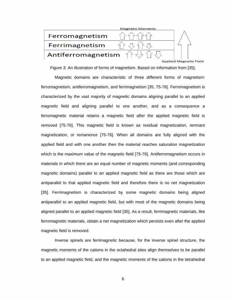
Figure 3: An illustration of forms of magnetism. Based on information from [35].

Magnetic domains are characteristic of three different forms of magnetism:

ferromagnetism, antiferromagnetism, and ferrimagnetism [35, 75-76]. Ferromagnetism is

characterized by the vast majority of magnetic domains aligning parallel to an applied

magnetic field and aligning parallel to one another, and as a consequence a

ferromagnetic material retains a magnetic field after the applied magnetic field is

removed [75-76]. This magnetic field is known as residual magnetization, remnant

magnetization, or remanence [75-76]. When all domains are fully aligned with the

applied field and with one another then the material reaches saturation magnetization

which is the maximum value of the magnetic field [75-76]. Antiferromagnetism occurs in

materials in which there are an equal number of magnetic moments (and corresponding

magnetic domains) parallel to an applied magnetic field as there are those which are

antiparallel to that applied magnetic field and therefore there is no net magnetization

[35]. Ferrimagnetism is characterized by some magnetic domains being aligned

antiparallel to an applied magnetic field, but with most of the magnetic domains being

aligned parallel to an applied magnetic field [35]. As a result, ferrimagnetic materials, like

ferromagnetic materials, obtain a net magnetization which persists even after the applied

magnetic field is removed.

Inverse spinels are ferrimagnetic because, for the inverse spinel structure, the

magnetic moments of the cations in the octahedral sites align themselves to be parallel

to an applied magnetic field, and the magnetic moments of the cations in the tetrahedral

7

sites align themselves to be antiparallel to an applied magnetic field [12]. On account of

this, the specific value of the magnetic moment of inverse spinel compounds depends on

the cations involved, which in this case are Cobalt (Co2+) and Iron (III) (Fe3+) [12]. On a

more macro level, as we previously described, there are twice as many occupied

octahedral sites as there are occupied tetrahedral sites, and therefore, in an applied

magnetic field, the unit cell acquires a net magnetization which is parallel to the applied

magnetic field [35].

On account of the remanence present in ferromagnetic and ferrimagnetic

materials, these materials possess hysteresis, which comes from a Greek word for

“lagging” [76].

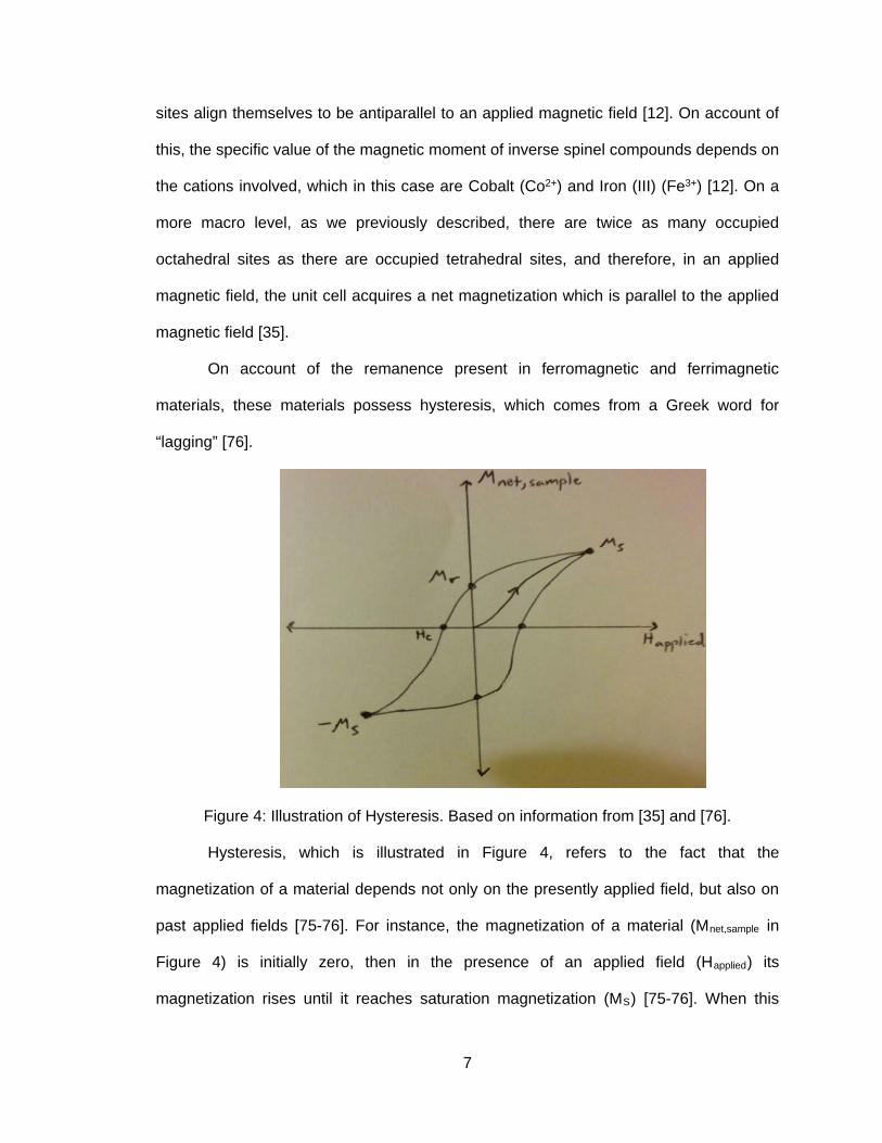
Figure 4: Illustration of Hysteresis. Based on information from [35] and [76].

Hysteresis, which is illustrated in Figure 4, refers to the fact that the

magnetization of a material depends not only on the presently applied field, but also on

past applied fields [75-76]. For instance, the magnetization of a material (Mnet,sample in

Figure 4) is initially zero, then in the presence of an applied field (Happlied) its

magnetization rises until it reaches saturation magnetization (MS) [75-76]. When this

8

applied field is removed, the magnetization reduces, but not to zero (which was the initial

state) rather to the level of remnant magnetization (Mr) [75-76]. In order to reduce the

magnetization to zero, a magnetic field must be applied opposite (or antiparallel) to the

remnant magnetization [75-76]. This applied magnetic field is known as a coercive

magnetic field, and its value is known as coercivity (HC) [75-76].

Superparamagnetism is characterized by zero hysteresis [35]. Specifically,

superparamagnetic materials align parallel to an applied magnetic field, and when that

field is removed they become non-magnetic, there is no remanence, and the magnetic

moments revert to random orientations [35]. Superparamagnetism only occurs at small

sizes because, at small sizes, room temperature thermal energy is sufficient to interfere

with magnetic moments and prevent them from maintaining their alignment in the

absence of an applied magnetic field [35]. Domain walls separate magnetic domains,

and as particle size decreases these domain walls are reduced and particles become

single domain [35]. Correspondingly, coercivity increases because moving domain walls

is a way of reversing magnetization and for single domain situations this is obviously not

an option for reversing magnetization [35]. Nevertheless, as particle size is reduced

further below the single domain threshold, one eventually reaches the point at which the

material becomes superparamagnetic and consequently the coercivity becomes zero

[35].

Hard magnetic materials have both high saturation magnetization and high

coercivity and thus they have wide hysteresis loops [35]. Soft magnetic materials have

high saturation magnetization and low coercivity and therefore they have narrow

hysteresis loops [35-36]. Cobalt Ferrite is a hard magnetic material [7, 11]. However,

several other spinel ferrites are soft magnetic materials [36]. Evidently, the magnetic

properties of Cobalt Ferrite nanoparticles differ from the bulk properties. Specifically, as

9

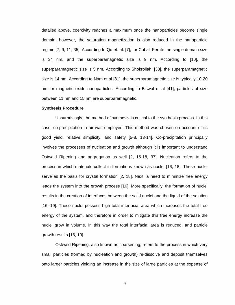
detailed above, coercivity reaches a maximum once the nanoparticles become single

domain, however, the saturation magnetization is also reduced in the nanoparticle

regime [7, 9, 11, 35]. According to Qu et. al. [7], for Cobalt Ferrite the single domain size

is 34 nm, and the superparamagnetic size is 9 nm. According to [10], the

superparamagnetic size is 5 nm. According to Shokrollahi [38], the superparamagnetic

size is 14 nm. According to Nam et al [81], the superparamagnetic size is typically 10-20

nm for magnetic oxide nanoparticles. According to Biswal et al [41], particles of size

between 11 nm and 15 nm are superparamagnetic.

Synthesis Procedure

Unsurprisingly, the method of synthesis is critical to the synthesis process. In this

case, co-precipitation in air was employed. This method was chosen on account of its

good yield, relative simplicity, and safety [5-8, 13-14]. Co-precipitation principally

involves the processes of nucleation and growth although it is important to understand

Ostwald Ripening and aggregation as well [2, 15-18, 37]. Nucleation refers to the

process in which materials collect in formations known as nuclei [16, 18]. These nuclei

serve as the basis for crystal formation [2, 18]. Next, a need to minimize free energy

leads the system into the growth process [16]. More specifically, the formation of nuclei

results in the creation of interfaces between the solid nuclei and the liquid of the solution

[16, 19]. These nuclei possess high total interfacial area which increases the total free

energy of the system, and therefore in order to mitigate this free energy increase the

nuclei grow in volume, in this way the total interfacial area is reduced, and particle

growth results [16, 19].

Ostwald Ripening, also known as coarsening, refers to the process in which very

small particles (formed by nucleation and growth) re-dissolve and deposit themselves

onto larger particles yielding an increase in the size of large particles at the expense of

10

small particles in solution [17-18, 37]. This occurs because small particles are more

soluble and they collectively have a greater surface area than large particles and

therefore a greater surface energy. Clearly, Ostwald Ripening is another process by

which the system reduces its overall free energy by reducing its total surface area [17-

18]. In order for co-precipitation to occur a solution needs to be brought to super-

saturation, and, in this research project, this was done by setting reaction temperature to

lead to super-saturation [2, 16, 18].

Based on the work of [7-8, 20] and others it is evident that increasing reaction

temperature yields an increase in average particle size. Also, a higher solution pH tends

to result in larger particles [8].

Two drawbacks of co-precipitation are that controlling the size distribution of the

fabricated particles can be difficult, and that the size distribution tends to be rather wide

meaning that the particles tend to be rather polydisperse [38-39].

Next, let us describe aggregation. Aggregation refers to the clustering or

clumping together of multiple particles. Clearly, this tends to increase average particle

size [13, 15, 17-18, 22-24]. Particles in solution are affected by Brownian motion [13, 15,

17-18, 22-24]. Consequently, particle collisions result and van der waals forces between

particles serve as an attractive force between the particles [13, 15, 17-18, 22-24].

Likewise, magnetic attraction between particles promotes aggregation [22]. These

attractive forces must be balanced by a repulsive force or else aggregation will result

[13, 15, 17-18, 22-24]. An example of a repulsive force is the electrostatic force between

particles in solution. This involves particle surface charge and corresponding zeta

potential, and is influenced by the pH of the solution and the ionic strength of the solution

[13, 15, 17-18, 22-24]. Another example, are steric forces which create a physical barrier

rather than an electric barrier to aggregation [13, 15, 17-18, 22-24]. An increase in ionic

11

strength reduces the thickness of the electric double layer around each particle, thereby

reducing the electrostatic repulsive force as well as the zeta potential, and consequently

leading to greater aggregation [13, 15, 17-18, 22-24]. An increase in stir rate will lead to

smaller particles [27]. Nanoparticle surfaces can be modified by capping agents in order

to decrease surface energy or increase steric hindrance [13, 15, 17-18, 22-24]. Both of

these measures reduce the tendency of the particles to aggregate [13, 15, 17-18, 22-24].

Oleic acid is a hydrophobic surfactant [21]. As a surfactant, it possesses a critical

micelle concentration (CMC), this means that above this specific concentration micelles

will form in solution [47-48]. Micelles are aggregates of surfactant particles and the

micelle properties depend on the surfactant concentration as well as the surrounding

medium [45]. Additionally, micelles contribute to the overall ionic strength of the solution

[46]. On account of this as well as the fact that the formation of micelles may reduce the

tendency of the nanoparticles to be coated by the surfactant molecules, when one is

interested in coating nanoparticles with a surfactant, it may be advisable to use a

surfactant concentration less than CMC. Nevertheless, this is not clear, and it seems

that it is possible to use a surfactant concentration which is greater than the CMC for

coating as long as a washing step(s) specifically designed to remove excess surfactant

is included [37].

Regarding factors which influence the average particle size of Cobalt Ferrite

nanoparticles, Co2+ concentration has been shown by Ayyappan et al [40] and Biswal et

al [41] to be an important factor. They found that Co2+ concentration and average Cobalt

Ferrite particle size are inversely related. In addition, Ayyappan et al [40] found that

coercivity and saturation magnetization are similarly related to the Co2+ concentration.

This matches with the findings of Pereira et al [42] who found that saturation

magnetization tends to decrease with decreasing particle size. Furthermore, there is

12

something called digestion time which refers to the time one waits after the reaction

temperature is reached before adding Oleic acid to the solution [37]. Ayyapan et al [37]

found that average particle size increased from 14 nm to 19 nm as the digestion time

was increased from 1 min to 120 min whereas the saturation magnetization decreased

(which again corresponds to the findings of Pereira et al [42] that decreasing particle

size leads to decreasing saturation magnetization).

Cobalt Ferrite nanoparticles are toxic because they induce oxidative stress which

refers to an imbalance between reactive oxygen species or reactive nitrogen species

and antioxidant defenses [43]. This imbalance eventually leads to DNA damage, cellular

apoptosis, and mutagenesis [43]. Different cell lines display different viability responses

to Cobalt Ferrite nanoparticles on account of differing interactions between the

nanoparticles and the cells, specifically based on different endocytic pathways [43].

Another source of toxicity is that Co2+ ions can leach from CoFe2O4, and these ions are

toxic [29]. Due to these sources of toxicity, in order to utilize Cobalt Ferrite nanoparticles

for medical applications one must coat the particles with a nontoxic, biocompatible

coating. Potential biocompatible coatings include certain polymers such as polyethylene

glycol (PEG) [30]. Another biocompatible polymer which can be used to coat Cobalt

Ferrite is polyvinylpyrrolidone (PVP) [44]. In addition, PVP is water soluble and it has

applications in drug delivery [44].

Hypotheses

An increase in reaction time will lead to an increase in coarsening and therefore

an increase in polydispersity (meaning the size range will increase), and in average

particle size. Sodium citrate will be more effective in preventing the aggregation of small

particles [24]. PVP and Oleic acid will be more effective capping agents for larger

particles [24].

13

Results

DLS Data

The following results were obtained using Dynamic Light Scattering (DLS) on a

Wyatt DynaPro plate reader, and subsequently processed via one-way analysis of

variance (ANOVA) as well as through post hoc tests using IBM SPSS. A 5% significance

level was used. In a like manner, Welch’s test was used in cases in which Levene’s test

indicated that the variances could not be assumed to be equal [82-83]. This happened

very frequently, presumably owing to the unequal sample sizes employed because

certain batches were analyzed more closely, through DLS, than others. More concretely,

the sample size for Control1 was thirty measurements, for PVP, Citrate, 1hr, and Oleic

the sample size was twenty measurements each, and for all other batches the sample

size was ten measurements each. On account of this, Tamhane’s test and Games-

Howell test were used as the post hoc tests [82-83].

The above equation, from [98], is used to calculate the ionic strength of a

solution. Clearly, changing the concentration of ionic reactants in solution will alter the

ionic strength. The difference between PVP particles and PVP 723 particles is the

quantity of reactants used and consequently the ionic strength is less for the PVP 723

particles. The only difference between CL particles and PVP particles are that the PVP

particles contain PVP.

In what follows, “hydrodynamic radius” refers to the population mean of the

hydrodynamic radius, and a “significant difference” refers a significant difference

between population means of hydrodynamic radii [83].

14

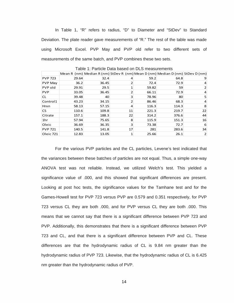
In Table 1, “R” refers to radius, “D” to Diameter and “StDev” to Standard

Deviation. The plate reader gave measurements of “R.” The rest of the table was made

using Microsoft Excel. PVP May and PVP old refer to two different sets of

measurements of the same batch, and PVP combines these two sets.

Table 1: Particle Data based on DLS measurements Mean R (nm) Median R (nm) StDev R (nm) Mean D (nm) Median D (nm) StDev D (nm)

PVP 723 29.64 32.4 4 59.2 64.8 9PVP May 36.2 36.45 2 72.4 72.9 4PVP old 29.91 29.5 1 59.82 59 2PVP 33.05 36.45 2 66.11 72.9 4CL 39.48 40 3 78.96 80 5Control1 43.23 34.15 2 86.46 68.3 4Hrxn 58.13 57.15 4 116.3 114.3 8CS 110.6 109.8 11 221.3 219.7 22Citrate 157.1 188.3 22 314.2 376.6 441hr 57.94 75.65 8 115.9 151.3 16Oleic 36.69 36.35 3 73.38 72.7 6PVP 721 140.5 141.8 17 281 283.6 34Oleic 721 12.83 13.05 1 25.66 26.1 2

For the various PVP particles and the CL particles, Levene’s test indicated that

the variances between these batches of particles are not equal. Thus, a simple one-way

ANOVA test was not reliable. Instead, we utilized Welch’s test. This yielded a

significance value of .000, and this showed that significant differences are present.

Looking at post hoc tests, the significance values for the Tamhane test and for the

Games-Howell test for PVP 723 versus PVP are 0.579 and 0.351 respectively, for PVP

723 versus CL they are both .000, and for PVP versus CL they are both .000. This

means that we cannot say that there is a significant difference between PVP 723 and

PVP. Additionally, this demonstrates that there is a significant difference between PVP

723 and CL, and that there is a significant difference between PVP and CL. These

differences are that the hydrodynamic radius of CL is 9.84 nm greater than the

hydrodynamic radius of PVP 723. Likewise, that the hydrodynamic radius of CL is 6.425

nm greater than the hydrodynamic radius of PVP.

15

The difference between PVP 721 and Oleic 721 is the use of PVP or Oleic acid

as the respective capping agent. Similarly, the difference between Citrate and Oleic is

the use of Citrate or Oleic acid as the respective capping agent. The Levene’s test

indicated that the variances between these batches are not equal. Therefore, as before,

we employed Welch’s test which yielded a significance value of .000, and this indicates

that significant differences are present. Looking at post hoc tests, the significance values

for the Tamhane test and for the Games-Howell test for PVP 721 versus Oleic 721 are

both .000, for Citrate versus Oleic they are both .000, for Citrate versus CS they are both

.000, for Oleic versus CS they are both .000 as well, and for Oleic versus Control1 they

are .196 and .133 respectively. This indicates that there are significant differences

between PVP 721 and Oleic 721, between Citrate and Oleic, between Citrate and CS,

and between Oleic and CS. However, there is not enough evidence to indicate a

significant difference between Oleic and Control1.

The difference between 1hr, Control1, and Hrxn are only the reaction times. The

reaction times for these three batches are one hour, two hours, and three hours

respectively. The Levene’s test indicated that the variances between these 3 batches of

particles are not equal. As a result, again Welch’s test was used. Its significance value

was found to be .000. This suggests that significant differences are present. Looking at

post hoc tests, the significance values for the Tamhane test and for the Games-Howell

test for 1hr versus Control1 are .111 and .079 respectively, for 1hr versus Hrxn they are

both 1.000, and for Hrxn versus Control1 they are both .000. This stipulates that we do

not have the evidence to say that there is a significant difference between Control1 and

1hr or between Hrxn and 1hr; however, there is a significant difference between Hrxn

and Control1.

16

AFM Data

A Veeco Multimode Atomic Force Microscope, equipped with a Silicon AFM

probe labeled “Multi75M-G,” and NanoScope software was employed for Atomic Force

Microscopy (AFM) imaging and Magnetic Force Microscopy (MFM) imaging. MFM

imaging detects magnetic force gradients to generate images, and it also provides an

approximation of these gradients [90]. For instance, MFM imaging can measure

approximate values of the phase difference between the drive voltage (supplied by the

instrument) and the cantilever response (based on the sample), and this difference

corresponds to a shift in the resonant frequency of the cantilever [90]. This shift is itself

proportional to the strength of magnetic force gradients in the sample [90]. Thus, a

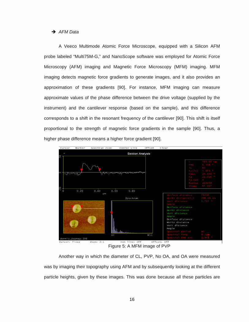
higher phase difference means a higher force gradient [90].

Figure 5: A MFM image of PVP

Another way in which the diameter of CL, PVP, No OA, and OA were measured

was by imaging their topography using AFM and by subsequently looking at the different

particle heights, given by these images. This was done because all these particles are

17

spherical or approximately spherical and therefore a height measurement on the AFM

will give a good measurement of their diameters [88-89].

Figure 6: An AFM image of PVP

Figure 7: Different AFM Image of PVP

18

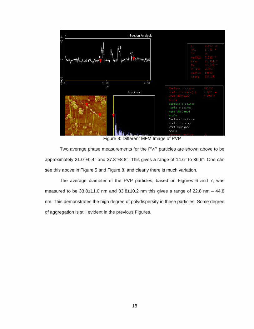
Figure 8: Different MFM Image of PVP

Two average phase measurements for the PVP particles are shown above to be

approximately 21.0°±6.4° and 27.8°±8.8°. This gives a range of 14.6° to 36.6°. One can

see this above in Figure 5 and Figure 8, and clearly there is much variation.

The average diameter of the PVP particles, based on Figures 6 and 7, was

measured to be 33.8±11.0 nm and 33.8±10.2 nm this gives a range of 22.8 nm – 44.8

nm. This demonstrates the high degree of polydispersity in these particles. Some degree

of aggregation is still evident in the previous Figures.

19

Figure 9: AFM image of CL. Notice the high amount of aggregation.

Figure 10: An MFM image of CL

For the CL particles the average phase difference ranges from 15.8° to 27.8°.

This can be seen in Figure 10; it is also evident that the phase difference varies widely

owing to the large amount of aggregation. The average diameter for the CL particles,

shown in Figure 9, ranges from 51.2 nm – 108.6 nm. The aggregation is clear here in

that a greater degree of aggregation tends to yield a larger average diameter.

20

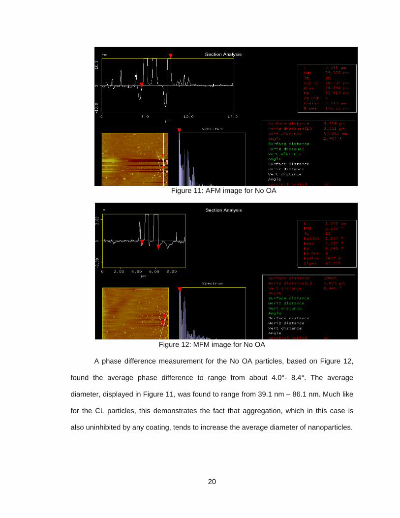
Figure 11: AFM image for No OA

Figure 12: MFM image for No OA

A phase difference measurement for the No OA particles, based on Figure 12,

found the average phase difference to range from about 4.0°- 8.4°. The average

diameter, displayed in Figure 11, was found to range from 39.1 nm – 86.1 nm. Much like

for the CL particles, this demonstrates the fact that aggregation, which in this case is

also uninhibited by any coating, tends to increase the average diameter of nanoparticles.

21

Figure 13: OA On the Left, AFM Image; On the Right, MFM Image. Dipoles

(seen as dark to light or vice versa) are clearly visible in the MFM image.

Figure 14: Closer View of AFM image for OA

22

Figure 15: Closer View of MFM image for OA

Figure 16: Another AFM image for OA

23

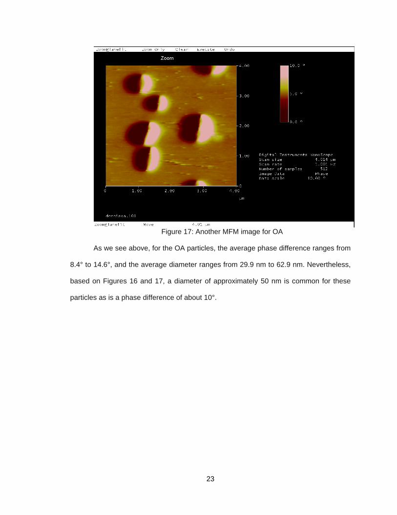
Figure 17: Another MFM image for OA

As we see above, for the OA particles, the average phase difference ranges from

8.4° to 14.6°, and the average diameter ranges from 29.9 nm to 62.9 nm. Nevertheless,

based on Figures 16 and 17, a diameter of approximately 50 nm is common for these

particles as is a phase difference of about 10°.

24

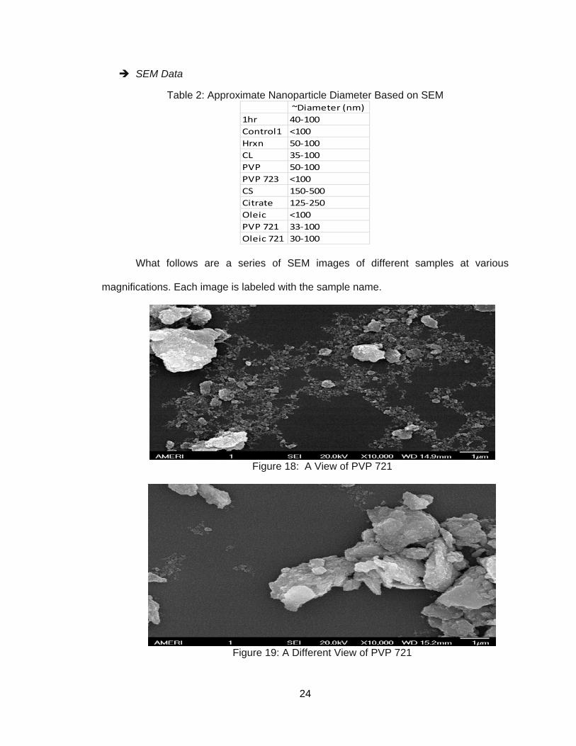
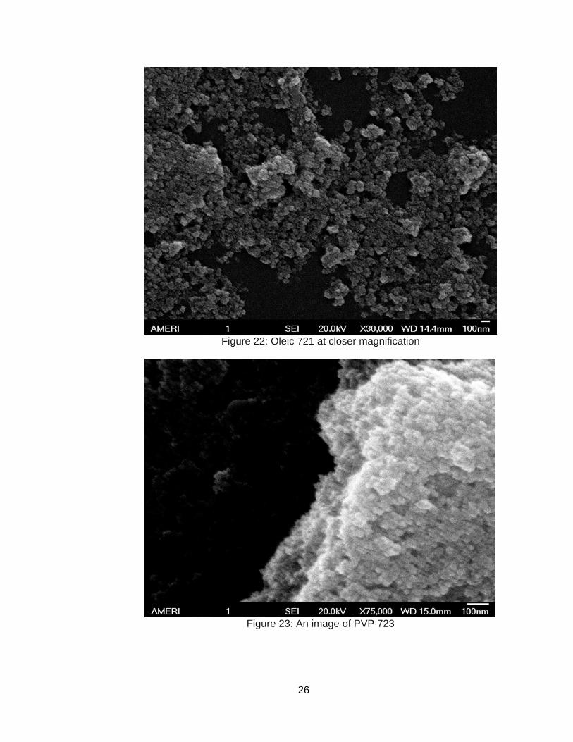
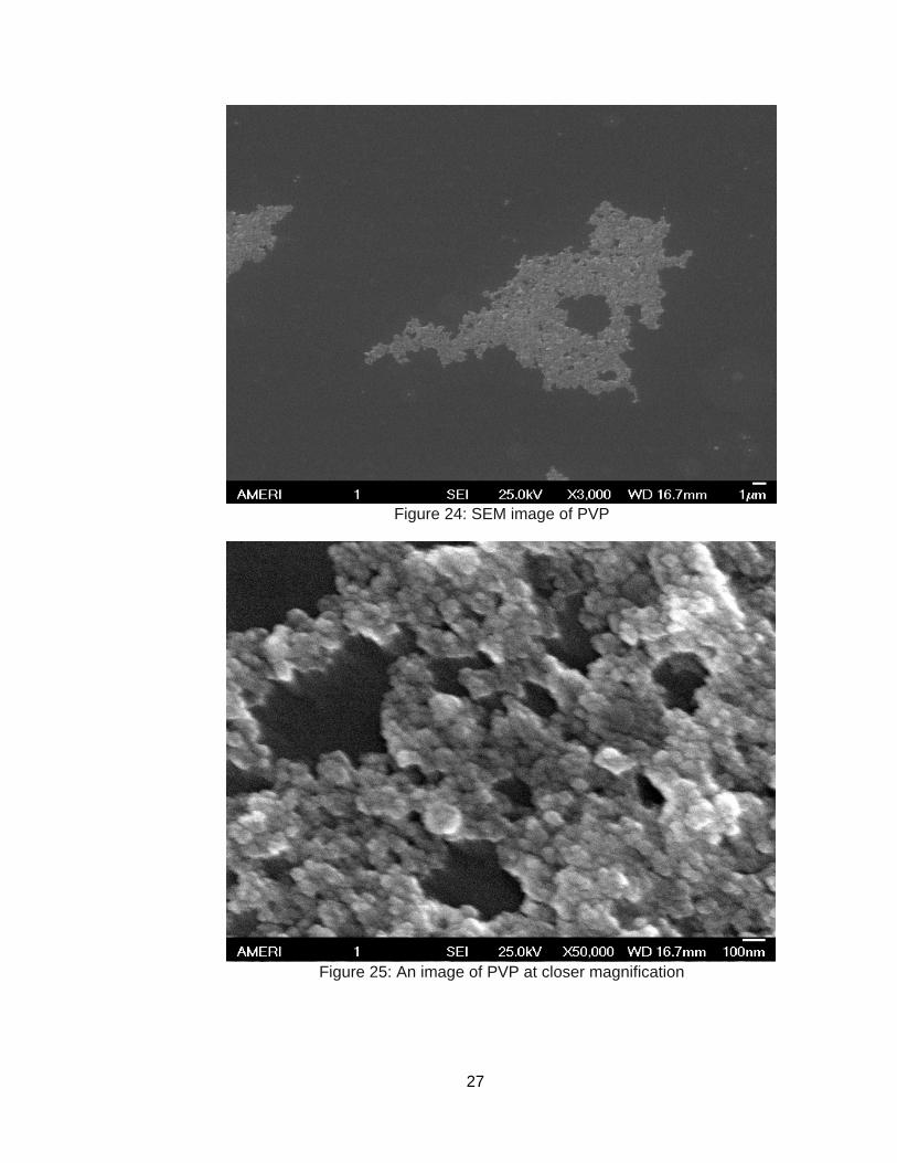
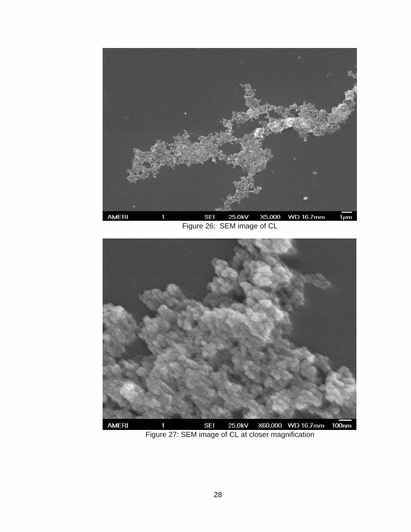
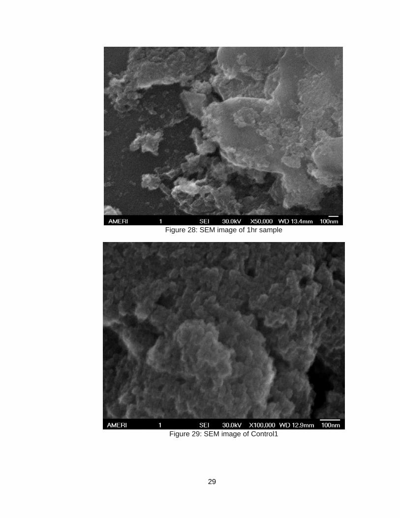
SEM Data

Table 2: Approximate Nanoparticle Diameter Based on SEM ~Diameter (nm)

1hr 40-100Control1 <100Hrxn 50-100CL 35-100PVP 50-100PVP 723 <100CS 150-500Citrate 125-250Oleic <100PVP 721 33-100Oleic 721 30-100

What follows are a series of SEM images of different samples at various

magnifications. Each image is labeled with the sample name.

Figure 18: A View of PVP 721

Figure 19: A Different View of PVP 721

25

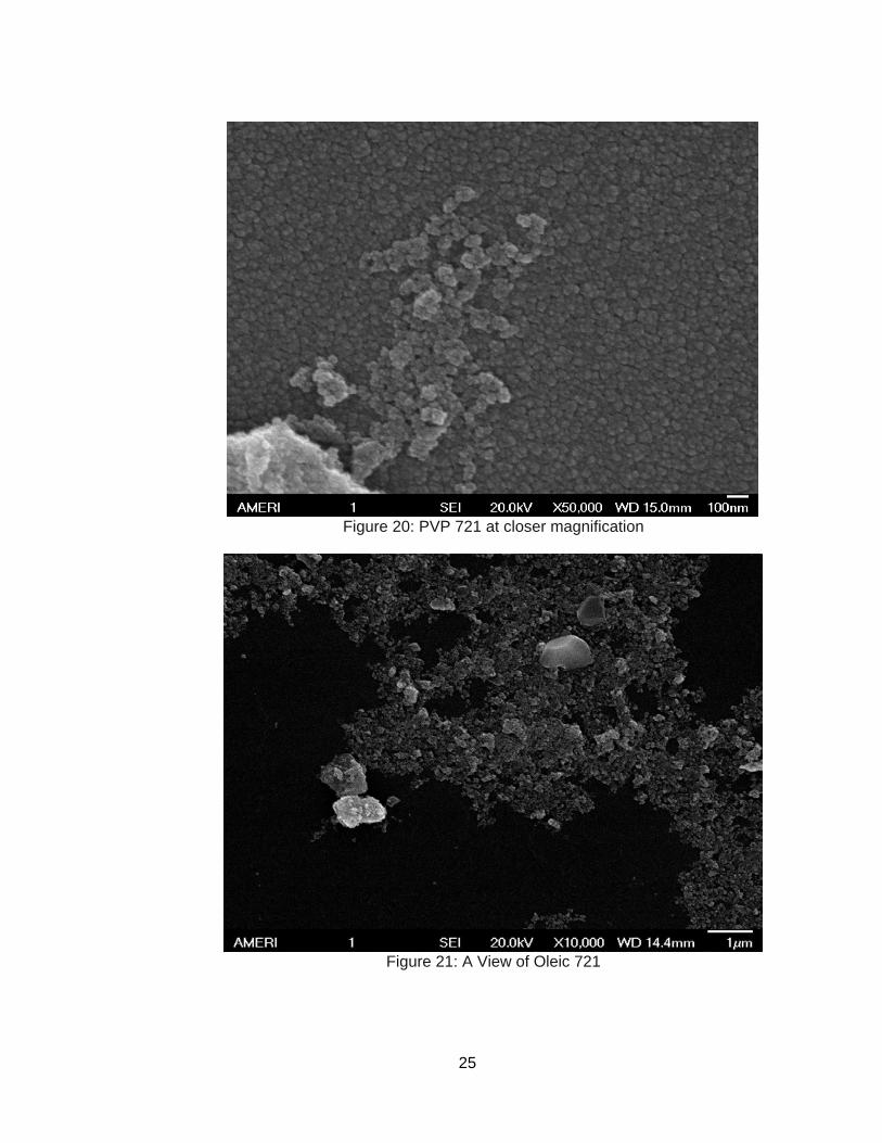
Figure 20: PVP 721 at closer magnification

Figure 21: A View of Oleic 721

26

Figure 22: Oleic 721 at closer magnification

Figure 23: An image of PVP 723

27

Figure 24: SEM image of PVP

Figure 25: An image of PVP at closer magnification

28

Figure 26: SEM image of CL

Figure 27: SEM image of CL at closer magnification

29

Figure 28: SEM image of 1hr sample

Figure 29: SEM image of Control1

30

Figure 30: SEM image of the sample labeled Oleic

Figure 31: SEM image of Hrxn

31

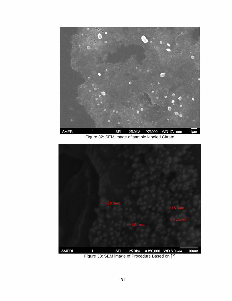
Figure 32: SEM image of sample labeled Citrate

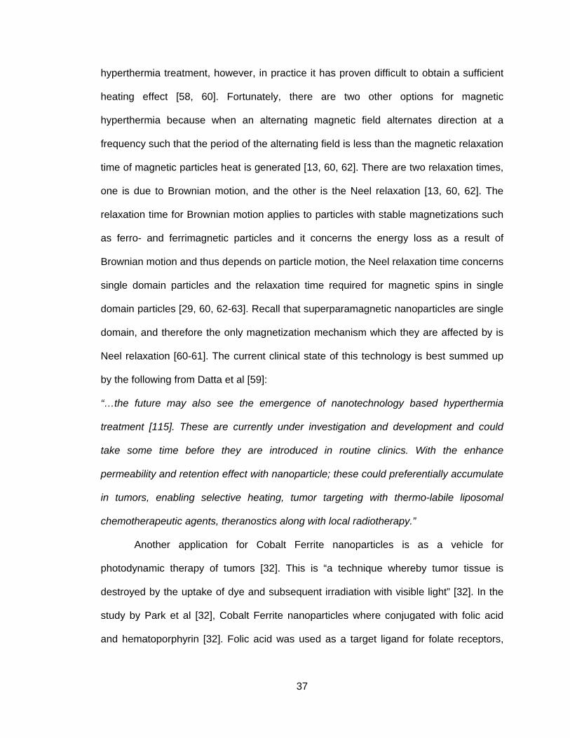
Figure 33: SEM image of Procedure Based on [7]

32

Discussion

All the SEM images show considerable aggregation, however, there is a

noticeable, albeit slight, reduction in aggregation for PVP as compared to CL. PVP 723

is more aggregated than PVP. This could be because of an error in sample preparation.

1hr, Control1, Oleic, and Hrxn all look similar. Hrxn has the clearest image. The author is

not certain why this is; again perhaps the sample preparation was better for Hrxn as

compared to the other three. The SEM image for Citrate (Figure 32) shows its large

particle size.

The SEM measurements of particle size for Oleic 721 and PVP 721 are similar;

however, the PVP 721 SEM images appear more clustered than the Oleic 721 SEM

images.

Figure 33 is an SEM image of a batch of particles fabricated according to a

procedure similar to [7] at 100°C with a 100 mL solution, containing 0.6 g of Iron (III)

nitrate nonahydrate and 0.22 g of Cobalt (II) nitrate hexahydrate, being drop-by-drop

added to a 50 mL solution, containing 1.6 g of Sodium Hydroxide. The stir rate ranged

from 300-600 RPM, and the reaction time was 2 hours. Figure 33 shows aggregation but

also enough separation to be able to measure some particles in the range of 18 nm – 30

nm. Qu et al [7], measured an average particle diameter of 47 nm for 100°C. Our

average diameter is less probably because we employed less metal reactants, less total

volume of solution, and because [7]’s procedure did not specify the stir rate which one

should utilize. Also, we washed the particles in a different way than did Qu et al [7].

The fact that there is not enough evidence to indicate a significant difference

between Control1 and 1hr is interesting, and perhaps explains why some procedures,

such as [40], [41], and others, rely on a reaction time which is shorter than two hours.

Regarding the finding that there is a significant difference between Hrxn and Control1,

33

the author is not certain why this is, but perhaps it is on account of a longer period of

coarsening which results in larger particles and more polydisperse particles. Thanh et al

[92] had similar findings, more specifically, in that case nanoparticle size and

polydispersity increased with increasing reaction time on account of Ostwald ripening.

Moving on, the result that there is insufficient data to demonstrate a significant

difference between Oleic and Control1 is probably on account of the volume of Oleic

Acid used to fabricate Oleic. The volume used was only about 22 μL. Furthermore, it

was added in before the addition of Potassium Hydroxide and before the reaction

temperature was reached, and perhaps this reduced its effectiveness.

Moreover, our results demonstrating a significant difference between both PVP

723 and CL along with PVP and CL demonstrate that PVP introduces steric hindrance

which leads to a lower aggregation tendency and a lower measured hydrodynamic

radius for the coated particles. This is what we expected. Likewise, we obtained a similar

result utilizing AFM imaging of CL. Furthermore, the fact that we failed to find a

significant difference between PVP 723 and PVP indicates that the ionic strength

difference between these two batches was not a significant factor. MFM imaging

indicated a similar distribution of magnetic force gradients for PVP coated particles and

for CL. This shows that the PVP coating did not greatly alter the magnetic force

gradients. The coating made the gradients more visible by reducing aggregation. A

similar result can be seen for the magnetic force gradients of OA versus No OA, and

regarding the AFM findings concerning OA and No OA, the addition of Oleic acid clearly

was effective in reducing aggregation.

Next, the DLS measurements of PVP 721, CS, and Citrate are very large. An

explanation for the hydrodynamic radius of PVP 721 is unclear. It is most likely an error

in the DLS measurement. The large size of CS can be accounted for by the fact that the

34

procedure utilized proved to be a failure because it yielded a final colloid with a pH of

only 5.7, which is far below the recommended pH range of 8.5 or greater [8]. This pH

was measured using an Oakton pH 11 series meter, and the fact that it is very acidic

could have led to this very large size. In addition, according to Sodaee et al [93], a pH of

at least 8 is needed to yield Cobalt Ferrite. Therefore, CS is not even a sample of Cobalt

Ferrite, but is in fact mostly goethite [93]. The case of Citrate is a similar situation in the

sense that the procedure was a failure, however, in this particular case the pH was not

the issue. The issue is simply that it appears that Trisodium Citrate cannot be used as a

capping agent for Cobalt Ferrite nanoparticles prepared via co-precipitation in air, and

therefore our hypothesis in this regard is false. Maybe, it would be possible to use Citric

Acid as a capping agent instead, and one could follow a procedure similar to that used

by Goodarzi et al [84] or A.B. Shinde [85].

The above comes from [93] and [94]. On the left are the chemical equations and

the general reaction mechanism for No OA, and on the right is an outline of a general

reaction mechanism for a process to fabricate Cobalt Ferrite with an Iron (II) compound

35

rather than an Iron (III) compound, such as Iron (III) Nitrate Nonahydrate (which is what

was used in all the procedures of this thesis). If we look at [96], which utilizes Iron (II)

Dodecyl Sulfate and a microemulsion method to produce Cobalt Ferrite nanoparticles we

can see that the diameter of their fabricated particles is between 2 nm and 5 nm. It is

probable that the significantly lower degree of polydispersity of these results is due to the

method of microemulsions, however, the small size is not only confined to the method of

microemulsions. Gyergyek et al [95], synthesized Cobalt Ferrite nanoparticles with a

diameter of about 8 nm using Iron (II) Sulfate Heptahydrate and co-precipitation. In the

above equations, it is evident that the process on the right involves more

reactions/steps. If we examine the structure of Cobalt Ferrite, we know that, for Cobalt

Ferrite, the final oxidation state of iron is 3+ and not 2+. For this reason, if an Iron (II)

compound is used to fabricate Cobalt Ferrite, the compound must undergo oxidation

before it can enter nucleation [96-97]. This accounts for the additional reactions/steps,

and this lowers the nucleation rate for this process [96-97]. As a consequence, this

process is a nucleation dominated process that can be described, at least in part, by a

LaMer mechanism [26]. The result of this is that the process on the right produces less

polydisperse particles than the particles which are produced by the process on the left

[26]. Nevertheless, in the end, a nanoparticle size distribution depends largely on the

specifics of the synthesis procedure employed.

Applications

Passive targeting relies upon the fact that tumors and other inflamed tissues

have poor vasculatures as well as the reality that they lack the capacity for lymphatic

drainage [64, 78]. This allows long-circulating nanoparticles to eventually penetrate and

to accumulate in these tissues [64, 78]. This is known as enhanced permeability and

retention (EPR) effect [64, 78].

36

Active targeting involves functionalizing the surface of nanoparticles with a

targeting ligand or multiple targeting ligands which are selected based on their binding

affinity for the cell surface receptors of the cells one is interested in targeting [64, 66-67,

78]. Nanoparticles can also sometimes be functionalized with a specific ligand(s) which

leads to specific binding and nanoparticle internalization through receptor-mediated

endocytosis [64]. Nanoparticles can be used for drug delivery by functionalizing a

specific drug to the surface of the nanoparticles in addition to other coatings, which could

include those to prevent aggregation, increase biocompatibility, increase hydrophilicity,

or targeting ligands [64-65, 67, 78]. Using a combination of coatings, nanoparticles can

be targeted to specific cells, and drugs can be delivered in a more targeted way than by

simply applying free drug to an area [64-65, 67, 78]. An advantage that this has is

reduced toxicity to surrounding cells [78].

Hyperthermia is a cancer treatment which involves applying temperatures

between 41°C and 45°C to kill cancer cells [29-30, 59-61]. Typically treatments are

applied for at least thirty minutes [30]. Hyperthermia treatments can be carried out using

magnetic nanoparticles generally and CoFe2O4 nanoparticles in particular, in what is

called magnetic hyperthermia [29-30, 59-61]. When a high frequency alternating

magnetic field is applied to ferro- or ferrimagnetic nanoparticles a hysteresis loop is

generated for the particles [60]. For each cycle of this loop a quantity of electromagnetic

energy proportional to the area of the hysteresis loop is converted to heat in what are

called hysteretic losses [60-61]. These hysteretic losses arise from the breaking and

forming of domain walls (the walls between magnetic domains) as a result of the

magnetization being repeatedly alternated [62]. When these changes happen slower

than the applied magnetic field is alternated then heat is generated [13, 62]. Clearly,

these hysteretic losses are a potential way to generate the heat required for

37

hyperthermia treatment, however, in practice it has proven difficult to obtain a sufficient

heating effect [58, 60]. Fortunately, there are two other options for magnetic

hyperthermia because when an alternating magnetic field alternates direction at a

frequency such that the period of the alternating field is less than the magnetic relaxation

time of magnetic particles heat is generated [13, 60, 62]. There are two relaxation times,

one is due to Brownian motion, and the other is the Neel relaxation [13, 60, 62]. The

relaxation time for Brownian motion applies to particles with stable magnetizations such

as ferro- and ferrimagnetic particles and it concerns the energy loss as a result of

Brownian motion and thus depends on particle motion, the Neel relaxation time concerns

single domain particles and the relaxation time required for magnetic spins in single

domain particles [29, 60, 62-63]. Recall that superparamagnetic nanoparticles are single

domain, and therefore the only magnetization mechanism which they are affected by is

Neel relaxation [60-61]. The current clinical state of this technology is best summed up

by the following from Datta et al [59]:

“…the future may also see the emergence of nanotechnology based hyperthermia

treatment [115]. These are currently under investigation and development and could

take some time before they are introduced in routine clinics. With the enhance

permeability and retention effect with nanoparticle; these could preferentially accumulate

in tumors, enabling selective heating, tumor targeting with thermo-labile liposomal

chemotherapeutic agents, theranostics along with local radiotherapy.”

Another application for Cobalt Ferrite nanoparticles is as a vehicle for

photodynamic therapy of tumors [32]. This is “a technique whereby tumor tissue is

destroyed by the uptake of dye and subsequent irradiation with visible light” [32]. In the

study by Park et al [32], Cobalt Ferrite nanoparticles where conjugated with folic acid

and hematoporphyrin [32]. Folic acid was used as a target ligand for folate receptors,

38

which are overexpressed in human cancer cells, and hematoporphyrin played the role of

the “dye” described previously [32].

In the presence of a magnetic field (B), a torque (τ) is generated on magnetic

moments (μ) given by the following equation [72]:

𝜏𝜏 = 𝜇𝜇 × 𝐵𝐵

And by the definition of the cross product:

‖𝜏𝜏‖ = ‖𝜇𝜇‖‖𝐵𝐵‖ sin𝜃𝜃

Another important formula is given below:

𝜔𝜔𝐿𝐿 = −𝛾𝛾𝐵𝐵

This formula defines a quantity known as the larmor frequency (ωL) which we will

describe later on [72].

As you can see this torque depends on the sine of the polar angle (θ) between

the magnetic field vector and the magnetic moment vector. As a consequence, when this

polar angle is 0° or 180° (π radians) then the magnetic moment will not experience any

torque. In all other circumstances, the magnetic moment, in an applied magnetic field,

will experience a torque. However, as can be seen, the larmor frequency does not

depend on this polar angle.

In an applied magnetic field along the z-axis, the net magnetization of the nuclei

of a sample will align with the field, however, this alignment is not perfect [69-70]. A

majority of the magnetic moments of the protons will be aligned parallel to the applied

magnetic field, and the rest of the moments will be aligned antiparallel to the applied

magnetic field [69-70]. Correspondingly, the majority of the quantum spins will be aligned

parallel to the applied magnetic field, and the rest will be aligned antiparallel to that field

[70]. This is the case because the lower energy state is the state parallel to the field and

therefore a majority of the spins and their corresponding magnetic moments favor this

39

orientation [69-71]. Keep in mind that the quantum spin state does not take a defined

value until it is observed [71]. As a result, it is useful for us to look at quantum spin as

the superposition of the spin up and spin down states, and doing so gives us the result

that the spin is actually rotating (or precessing) around the z-axis at a frequency known

as the larmor frequency [71]. A classical way of looking at this is that the magnetic

moments are not perfectly aligned with the z-axis, meaning that there is an angle

between the z-axis and the magnetic moments, and this results in the magnetic

moments feeling a torque which causes them to precess about the z-axis at a resonant

frequency which is the larmor frequency [70, 77].

If an oscillating magnetic field (B1) with an x and y component, oscillating at the

larmor frequency, is applied perpendicular to the net magnetic field (B0) then the

magnetic moments can be rotated 90° into the x-y plane, this causes an increase in the

energy of the sample [62, 69-70]. Or, the sample’s magnetic moments, through the

application of a different oscillating magnetic field (B1) without an x and y component at

the larmor frequency applied antiparallel to B0, can be flipped entirely which results in a

larger energy increase [62, 69-70]. The T2 relaxation time, or transverse relaxation time,

is the time it takes for the magnetic moments in the x-y plane to decay away, and the T1

relaxation time is the longitudinal relaxation time and it refers to the time that it will take

for the magnetic moments to return to their original longitudinal orientation (their original

z-direction) [69-70]. This changing of magnetic moments can be detected by the voltage

which it induces in pickup coils and based on this an image can be created [62, 69, 77].

Different tissues have different T1 and different T2 times [64, 69]. MRI machines typically

have gradient coils which change the applied magnetic field in certain regions in order to

increase spatial resolution because recall that the larmor frequency depends on the

applied field [73].

40

For MRI, T2 contrast agents lead to a darkening of the MRI image, and Cobalt

Ferrite nanoparticles have potential applications as such contrast agents [74]. T2

contrast agents are called negative imaging agents for this reason; they darken the MRI

image by shortening the T2 relaxation time and thereby increasing the contrast of the

MRI image [68-69, 77, 79]. The effectiveness of magnetic nanoparticles used as contrast

agents depends on (MsV)2 and d-6 where Ms is the saturation magnetization, V is the

nanoparticle volume and d is the distance from the protons to the nanoparticle surface

[69].

Processes and Tools

Measurement Tools

Dynamic light scattering (DLS) is a tool which is used to measure particle size,

specifically one can utilize it to obtain the hydrodynamic radius of particles [51-53]. DLS

treats all particles as spherical, and so the measured hydrodynamic radius will only be

an approximation if the particles being measured are not spherical [51-52]. The process

works by shining a laser through a solution of particles [51-53]. The particles in solution

are in constant motion, and as the laser shines over them it scatters and forms a speckle

pattern [51-52]. Based on the speckle pattern the instrument determines variations in the

intensity of the scattered light [51-52]. The variation of intensity with time can be used to

measure the diffusion coefficient of the particles [52]. Based on this, the hydrodynamic

radii of the particles can be determined using the Stokes-Einstein equation [52]. DLS

measurements tend to be larger than measurements obtained by TEM or SEM because

DLS measurements include a measurement of the adsorbing layer, which is made up of

a hydration or solvent layer and, for coated particles, can also include a coating layer

41

[51-52, 54]. Specifically, according to Sinko et al [55], “the size derived from DLS is two

to three times larger” than the size measured from SEM.

Scanning Electron Microscopy (SEM) functions by emitting an incident beam of

electrons onto a sample [56-57]. This leads to backscattered electrons and secondary

electrons [56-57]. The backscattered electrons have higher energies than the low energy

of secondary electrons, and the secondary electrons are more sensitive to surface

topology than the backscattered electrons [56-57]. The backscattered electrons are

useful for imaging samples with higher atomic weights and higher densities as a result of

the increased tendency for scattering events in these samples [56-57]. An area that

consists of a heavy atom appears bright in a backscattered electron image [80].

The electron gun in the SEM is a thermionic gun which emits thermoelectrons

from a tungsten filament by heating this filament to 2800 K [80]. These electrons are

directed by applying a positive voltage, with respect to the cathode, to a metal plate (the

anode) [80]. It relies on a “magnetic lens” that is composed of two coil wound electric

wires [80]. The inside of the specimen chamber and the SEM system must be kept at a

high vacuum of 10-3 to 10-4 Pa [80]. There is also a secondary electron detector

composed of a pair of electrodes known as a collector, as well as a scintillator, a photo-

multiplier tube (PMT), and an amplifier [80]. A large voltage is applied between the

electrodes of the collector (~50V-300V), and a larger voltage (10kV) is applied to the

scintillator [80]. This is done in order to attract secondary electrons towards the

scintillator where they are absorbed and reemitted as light which is sent towards the

PMT, multiplied, and converted back to electrons which form a current which is amplified

by the amplifier and detected as the signal of secondary electrons [80]. Brightness

variation depends on the number of secondary electrons detected [80]. SEM has a

massive advantage in the depth of field versus light microscopy [57]. The accelerating

42

voltage, which one can adjust while imaging, is related to the penetration depth; a higher

accelerating voltage leads to a higher penetration depth and correspondingly results in a

degraded view of the surface [57, 80]. In fact, a high accelerating voltage can damage a

sample’s surface [57]. Therefore, a low accelerating voltage is favorable for imaging the

specimen surface [80]. In conductive samples, the electrons which do not become

scattered pass through the sample and the specimen stage, however, in nonconductive

samples these electrons stop within the sample and provide a negative charge to a

particular part of the sample [80]. This is known as charging, and this eventually causes

the electron beam to be repelled and the image to be distorted [80].

An atomic force microscope (AFM) consists of an optical cantilever arm, a laser,

and a photodiode detector [86-87]. The device relies on electrostatic forces between the

atoms of the cantilever tip and the specimen [86-87]. This interaction leads to a

deflection of the tip, and this deflection can be measured by reflecting a laser beam off of

the optical cantilever arm and then measuring this reflection using the built-in photodiode

detector [86-87]. Magnetic force microscopy (MFM) is a secondary imaging mode, for

imaging magnetic materials, under Scanning Probe Microscopy (SPM), and it relies on

“the magnetic field’s dependence on tip-sample separation that induces changes in the

cantilever’s amplitude, resonance frequency, or phase” [87].

43

Materials

Sigma Aldrich Iron (III) nitrate nonahydrate

Sigma Aldrich Cobalt (II) nitrate hexahydrate

Sigma Aldrich Potassium Hydroxide, Sigma Aldrich Sodium Hydroxide

Sigma Aldrich Polyvinylpyrrolidone (PVP), Sigma Aldrich Oleic Acid, Sigma Aldrich

Trisodium Citrate Dihydrate

Methods

Initially, eight batches of Cobalt Ferrite nanoparticles were fabricated. What

follows is a description of the methods used.

For the batch labeled Control1, this procedure was done in a fume hood:

1.) Fill a beaker with 100 mL of deionized water.

2.) Place a stir bar into the beaker.

3.) Place the beaker onto the hot plate, which also has a stirring setting.

4.) Set the stirrer to 250 RPM.

5.) Add 0.8 grams of Cobalt (II) Nitrate Hexahydrate to the beaker.

6.) When the Cobalt (II) Nitrate Hexahydrate is dissolved, add 2.2 grams of Iron

Nitrate Nonahydrate to the beaker.

7.) When the Iron (III) Nitrate Nonahydrate is dissolved, set the temperature on

the hot plate to 75°C. This solution is known as the precursor solution.

8.) Fill a small beaker or a small Erlenmeyer flask with 10 mL of deionized water.

9.) Add approximately 2 grams of Potassium Hydroxide to the 10 mL solvent.

10.) Carefully swirl the beaker or the flask in order to dissolve the Potassium

Hydroxide.

44

11.) When the Potassium Hydroxide is dissolved and the precursor solution

has reached the reaction temperature (75°C), use an eyedropper to rather

quickly add the Potassium Hydroxide solution to the precursor solution, under

stirring. This should take about 5 minutes or less.

12.) Allow the solution to react for 2 hours, under stirring.

For the batch labeled 1hr the procedure used was the same as above except for

two changes. These were that the stir rate was changed from 250 RPM to 400 RPM,

and, most importantly, the reaction time was changed from 2 hours to 1 hour.

For the batch labeled Hrxn the procedure used was again the same as for

Control1, but for one change, the reaction time was changed from 2 hours to 3 hours.

For the batch labeled CL the changes made to the Control1 procedure included

that the stir rate was changed from 250 RPM to 100 RPM, and that the reaction

temperature was changed from 75°C to 90°C.

For the batch labeled PVP the procedure was the same as that for CL with the

following exceptions. First, an additional step was added: before the hot plate was set to

the reaction temperature (in this case 90°C), 0.8 grams of polyvinylpyrollidone (PVP)

was added to the precursor solution. The other change was that the reaction time was

less than 2 hours (it was between 1.5 hours and 2 hours).

For the batch labeled CS the changes made to the Control1 procedure included

that the stir rate was changed from 250 RPM to 400 RPM, the quantity of Potassium

Hydroxide employed was reduced from 2 grams to 1 gram, and the reaction temperature

was reduced from 75°C to 40°C.

For the batch labeled Citrate the changes made to the Control1 procedure

included that the stir rate was changed from 250 RPM to between 300 RPM and 400

RPM, the quantity of Potassium Hydroxide was reduced from 2 grams to 1.5 grams, and

45

the reaction temperature was reduced from 75°C to 60°C. A further change was the

addition of another step: like for the PVP batch, before the reaction temperature was set

on the hot plate, 0.44 grams of Trisodium Citrate were added to the precursor solution.

For the batch labeled Oleic the procedure utilized was the same as that for

Citrate, but with the difference that rather than, 0.44 grams of Trisodium Citrate being

added to the precursor solution, before the reaction, 22 μL of Oleic acid was added to

the precursor solution.

For the batch labeled Oleic 721 the procedure was the same as that for Oleic

with the following exceptions: the stir rate was set to 500 RPM, the quantity of Potassium

Hydroxide utilized was 2 grams as opposed to 1.5 grams, the amount of Oleic acid used

was increased to approximately between 0.08 mL and 0.1 mL, and the Oleic acid was

only added to the precursor solution once the solution reached the reaction temperature

(60°C) and not before. The Potassium Hydroxide was added rapidly in this process.

For the batch labeled PVP 721 the procedure was the same as that for Oleic 721

except that PVP was used rather than Oleic acid and the PVP was added to the

precursor solution before the reaction temperature was set (the same way it was done

for PVP). The Potassium Hydroxide was also added rapidly, but not as rapidly as for

Oleic 721, in this case.

For the batch labeled PVP 723 the procedure was the same as that for PVP with

the exception that 0.4 grams of Cobalt (II) Nitrate Hexahydrate, 1.1 grams of Iron (III)

Nitrate Nonahydrate, and 0.56 grams of PVP were used.

For the batch labeled OA, this procedure was done in a fume hood:

1.) Fill a beaker with 100 mL of deionized water.

2.) Place a stir bar into the beaker.

3.) Place the beaker onto the hot plate, which also has a stirring setting.

46

4.) Set the stirrer to 500 RPM.

5.) Add 0.8 grams of Cobalt (II) Nitrate Hexahydrate to the beaker.

6.) When the Cobalt (II) Nitrate Hexahydrate is dissolved, add 2.2 grams of Iron

(III) Nitrate Nonahydrate to the beaker.

7.) When the Iron (III) Nitrate Nonahydrate is dissolved, set the temperature on

the hot plate to 60°C. This solution is known as the precursor solution.

8.) Fill a small beaker or a small Erlenmeyer flask with 20 mL of deionized water.

9.) Add approximately 2.89 grams of Sodium Hydroxide to the 20 mL solvent.

10.) Carefully swirl the beaker or the flask in order to dissolve the Potassium

Hydroxide.

11.) When the Sodium Hydroxide is dissolved and the precursor solution has

reached the reaction temperature (60°C), use an eyedropper to add the

Sodium Hydroxide solution to the precursor solution, under stirring. Do this

quickly.

12.) After 5 minutes, add 0.08g (~94 μL) of Oleic acid.

13.) Allow the solution to react for 2 hours, under stirring.

The procedure for No OA has only one difference from that of OA and it is that for No

OA, no Oleic acid was added.

Once one follows these procedures, one will usually be left with a beaker which

contains a dark colored solution (dark brown or black). The other possibility is that one is

left with a beaker with a black powder inside. In either case, at this point, one must wash

the particles this is done, for the former case, by dividing the solution into centrifuge

tube(s) and centrifuging them at between 2000 and 3000 RPM for at least 5 to 10

minutes but most importantly until the solution turns clear or only slightly brown and a

dark mass of particles is clearly visible on the bottom of the tube(s). Then this solution

47

should be discarded, and the tube(s) should be filled with deionized water. For OA, the

tube was filled with ethyl alcohol for the first wash, in other words the first wash was

conducted with ethyl alcohol for OA. For the powder case, one proceeds directly to the

adding of the deionized water. Then the tube(s) should be vortexed and sonicated until

the solution darkens once more and the dark mass of particles at the bottom of the

tube(s) dissipates or greatly diminishes. Then the tube(s) should be centrifuged once

more, again until the solution turns clear or only moderately brown and the particles

gather on the bottom of the tube(s). It should then be discarded in order to complete the

wash. One can also conduct washes without using the centrifuge; in this case one uses

a very powerful magnet to separate out the particles. This magnet is placed underneath

a beaker filled with a solution containing magnetic nanoparticles, and after sometime the

particles will collect at the bottom and the remainder of the solution will be free of

particles and can be discarded. For the next wash, deionized water is added, the beaker

is shaken and/or sonicated so that the particles disperse into the solution and then one

proceeds with the previously described procedure.

When the washes are complete one can re-suspend all or only some of the

particles in a solution of one’s choosing, or one can dry all or only some of the particles

by re-suspending those one wishes to dry in deionized water, putting this solution in a

beaker, and then, inside of a fume hood, using a hot plate to evaporate the deionized

water away. At the end of the drying process, one is left with a black powder which one

must scrape from the beaker and collect together, as a precaution this should be done in

a fume hood as well.

48

References [1] A.J. Cole, V.C. Yang, A.E. David, "Cancer theranostics: the rise of targeted magnetic nanoparticles," Trends in Biotechnology, vol. 29, no. 7, pp. 323-332, July 2011. doi:10.1016/j.tibtech.2011.03.001 [2] B.L. Cushing, V.L. Kolesnichenko, C.J. O’Connor, “Recent Advances in the Liquid-Phase Synthesis of Inorganic Nanoparticles,” Chemical Reviews, vol. 104, no. 9, pp. 3893-3946, Oct. 2003. [3] S. Ayyappan, J. Phillip, B. Raj, “A facile method to control the size and magnetic properties of CoFe2O4 nanoparticles,” Materials Chemistry and Physics, vol. 115, pp. 712-717, Feb. 2009. [4] G.A. El-Shobaky et al, “Effect of preparation conditions on physicochemical, surface, and catalytic properties of cobalt ferrite prepared by coprecipitation,” Journal of Alloys and Compounds, vol. 493, pp. 415-422, Dec. 2009. [5] Z. Zi et al, “Synthesis and magnetic properties of CoFe2O4 ferrite nanoparticles,” Journal of Magnetism and Magnetic Materials, vol. 321, pp. 1251-1255, Nov. 2008. [6] S. Amiri, H. Shokrollahi, “The role of cobalt ferrite nanoparticles in medical science,” Materials Science and Engineering C, vol. 33, pp. 1-8, Sept. 2012. [7] Y. Qu et al, “The effect of reaction temperature on the particle size, structure, and magnetic properties of coprecipitated CoFe2O4 nanoparticles,” Materials Letters, vol. 60, pp. 3548-3552, April 2006. [8] P. Kuruva et al, “Size control and magnetic property trends in Cobalt Ferrite Nanoparticles Synthesized Using an Aqueous Chemical Route,” IEEE Trans. Magn., vol. 50, no. 1, Jan. 2014. [9] Y. Zhang et al, “Composition and properties of cobalt ferrite nano-particles prepared by the co-precipitation method,” Journal of Magnetism and Magnetic Materials, vol. 322, pp. 3470-3475, June 2010. [10] Y. Cedeño-Mattei et al, “Tuning of magnetic properties in cobalt ferrite nanocrystals,” Journal of Applied Physics, vol. 103, no. 07E512, March 2008.

49

[11] Z. Karimi, L. Karimi, H. Shokrollahi, “Nano-magnetic particles used in biomedicine: Core and coating materials,” Materials Science and Engineering C, vol. 33, pp. 2465-2475, Jan. 2013. [12] A.G. Kolhatkar et al, “Tuning the Magnetic Properties of Nanoparticles,” International Journal of Molecular Sciences, vol. 14, pp. 15977-16009, July 2013. [13] I. Sharifi, H. Shokrollahi S. Amiri, “Ferrite-based magnetic nanofluids used in hyperthermia applications,” Journal of Magnetism and Magnetic Materials, vol. 324, pp. 903-915, Oct. 2011. [14] M. Houshiar et al, “Synthesis of cobalt ferrite (CoFe2O4) nanoparticles using combustion, coprecipitation, and precipitation methods: A comparison study of size, structural, and magnetic properties,” Journal of Magnetism and Magnetic Materials, vol. 371, pp.43-48, July 2014. [15] S. Laurent et al, “Magnetic Iron Oxide Nanoparticles: Synthesis, Stabilization, Vectorization, Physicochemical Characterizations, and Biological Applications,” Chemical Reviews, vol. 108, no. 6, pp. 2064-2110, June 2007. [16] C.B. Carter, M.G. Norton, “Phase Boundaries, Particles, and Pores,” in Ceramic Materials Science and Engineering. New York, NY: Springer, 2007, ch. 15, sec. 8, pp. 276-277. [17] G. Oskam, “Metal oxide nanoparticles: synthesis, characterization and application,” J Sol-Gel Sci Techn, vol. 37, pp. 161-164, Feb. 2006. [18] N. T. K. Thanh, N. Maclean, S. Mahiddine, “Mechanisms of Nucleation and Growth of Nanoparticles in Solution,” Chemical Reviews, vol. 114, pp. 7610-7630, July 2014. [19] D. Meyers, “Surfaces and Interfaces: General Concepts,” in Surfaces, Interfaces, and Colloids: Principles and Applications, 2nd ed. Online: John Wiley & Sons, Inc, 1999, ch.2, pp. 8-19. [20] C.N. Chinnasamy et al, “Growth Dominant Co-Precipitation Process to Achieve High Coercivity at Room Temperature in CoFe2O4 Nanoparticles,” IEEE Trans. Magn., vol. 38, no. 5, Sept. 2002.

50

[21] A. Dey, M.K. Purkait, “Effect of fatty acid chain length and concentration on the structural properties of the coated CoFe2O4 nanoparticles,” Journal of Industrial and Engineering Chemistry, Sept. 2014 [22] E.M. Hotze, T. Phenrat, G.V. Lowry, “Nanoparticle Aggregation: Challenges to Understanding Transport and Reactivity in the Environment,” J. Environ. Qual, vol. 39, pp.1909–1924, Nov. 2010. [23] M. Di Marco et al, “Colloidal stability of ultrasmall superparamagnetic iron oxide (USPIO) particles with different coatings,” International Journal of Pharmaceutics, vol. 331, pp. 197-203, Nov. 2006. [24] J. Jiang, G. Oberdorster, P. Biswas, “Characterization of size, surface charge, and agglomeration state of nanoparticle dispersions for toxicological studies,” J Nanopart Res, vol 11, pp. 77–89, June 2008. [25] C.B. Carter, M.G. Norton, “Complex Crystal and Glass Structures,” in Ceramic Materials Science and Engineering. Online: Springer, 2007, ch. 7, sec. 2, pp. 101-102. [26] T. Sugimoto, “Underlying mechanisms in size control of uniform nanoparticles,” Journal of Colloid and Interface Science, vol. 309, pp.106-118, 2007. [27] P.C. Morais et al, “Synthesis and characterization of size-controlled cobalt-ferrite-based ionic ferrofluids,” Journal of Magnetism and Magnetic Materials, vol. 225, pp. 37-40, 2001. [28] T. Miyazaki, H. Jin, “Magnetic Anisotropy,” in The Physics of Ferromagnetism. Online: Springer, 2012, ch. 5, sec. 1, pp. 205-206. [29] S. Matsuda, et al, “Synthesis of cobalt ferrite nanoparticles using spermine and their effect on death in human breast cancer cells under an alternating magnetic field,” Electrochim. Acta (2015), http://dx.doi.org/10.1016/j.electacta.2015.06.108. [30] E. Mazario et al, “Magnetic Hyperthermia Properties of Electrosynthesized Cobalt Ferrite Nanoparticles.” J. Phys. Chem. C, vol. 117, pp. 11405-11411, May 2013. dx.doi.org/10.1021/jp4023025.

51

[31] D. Carta et al, “A Structural and Magnetic Investigation of the Inversion Degree in Ferrite Nanocrystals MFe2O4 (M = Mn, Co, Ni).” J. Phys. Chem. C, vol. 113, pp. 8606-8615, April 2009. [32] B. J. Park et al, “Photodynamic Anticancer Activities of Multifunctional Cobalt Ferrite Nanoparticles in Various Cancer Cells.” Journal of Biomedical Nanotechnology, vol. 11, no. 2, 226-235, 2015. [33] C.B. Carter, M.G. Norton, “Models, Crystals, and Chemistry” in Ceramic Materials Science and Engineering. New York, NY: Springer, 2007, ch. 5, sec. 1-6, pp. 71-80. [34] K. E. Sickafus, J. M. Wills, N. W. Grimes, “Spinel Compounds: Structure and Property Relations,” J. Am. Ceram. Soc., vol. 82, no. 12, pp. 3279 – 3292. 1999. [35] D. S. Mathew, R. Juang, “An overview of the structure and magnetism of spinel ferrite nanoparticles and their synthesis in microemulsions,” Chemical Engineering Journal, vol. 129, pp. 51-65, 2007. doi:10.1016/j.cej.2006.11.001. [36] C.B. Carter, M.G. Norton, “Using Magnetic Fields and Storing Data” in Ceramic Materials Science and Engineering. New York, NY: Springer, 2007, ch. 33, sec. 1-19, pp. 598-618. [37] S. Ayyappan, J. Philip, B. Raj, “Effect of Digestion Time on Size and Magnetic Properties of Spinel CoFe2O4 Nanoparticles,” J. Phys. Chem. C, vol. 113, pp. 590-596, 2009. [38] H. Shokrollahi et al, “Structure, synthetic methods, magnetic properties and biomedical applications of ferrofluids,” Materials Science and Engineering C, vol. 33, pp. 2476-2487. 2013. http://dx.doi.org/10.1016/j.msec.2013.03.028. [39] D. Kim et al, “Heat generation of aqueously dispersed CoFe2O4 nanoparticles as heating agents for magnetically activated drug delivery and hyperthermia,” Journal of Magnetism and Magnetic Materials, vol. 320, pp. 2390-2396, May 2008. doi:10.1016/j.jmmm.2008.05.023. [40] S. Ayyappan et al, “Influence of Co2+ Ion Concentration on the Size, Magnetic Properties, and Purity of CoFe2O4 Spinel Ferrite Nanoparticles,” J. Phys. Chem. C, vol. 114, pp. 6334-6341, 2010.

52

[41] D. Biswal et al, “Tuning of magnetic properties in cobalt ferrite by varying Fe2+ and Co2+ molar ratios,” Journal of Magnetism and Magnetic Materials, vol. 345, pp. 1-6, June 2013. http://dx.doi.org/10.1016/j.jmmm.2013.05.052. [42] C. Pereira et al, “Superparamagnetic MFe2O4 (M = Fe, Co, Mn) Nanoparticles: Tuning the Particle Size and Magnetic Properties through a Novel One-Step Coprecipitation Route,” Chem. Mater, vol. 24, pp. 1496-1504, March 2012. dx.doi.org/10.1021/cm300301c. [43] L. Horev-Azaria et al, “Predictive Toxicology of cobalt ferrite nanoparticles: comparative in-vitro study of different cellular models using methods of knowledge discovery from data,” Particle and Fibre Toxicology, vol. 10, no. 32, pp. 1-17, 2013. http://www.particleandfibretoxicology.com/content/10/1/32. [44] W. Chen et al, “Improved polyvinylpyrrolidone microneedle arrays with non-stoichiometric cyclodextrin,” J. Mater. Chem. B, vol. 2, pp. 1699-1705, 2014. DOI: 10.1039/c3tb21698e. [45] P. Letellier, A. Mayaffre, M. Turmine, “Micellar aggregation for ionic surfactant in pure solvent and electrolyte solution: Nonextensive thermodynamics approach,” Journal of Colloid and Interface Science, vol. 321, pp. 195-204, 2008. doi:10.1016/j.jcis.2008.01.030. [46] N. Jalsenjak, “Contribution of micelles to ionic strength of surfactant solution,” Journal of Colloid and Interface Science, vol. 293, pp. 230-239, 2006. doi:10.1016/j.jcis.2005.06.030. [47] L. M. Bergstrom, “Explaining the growth behavior of surfactant micelles,” Journal of Colloid and Interface Science, vol. 440, pp. 109-118, 2014. http://dx.doi.org/10.1016/j.jcis.2014.10.054. [48] K. Kaibara et al, “Dispersion behavior of oleic acid in aqueous media: from micelles to emulsions,” Colloid Polym Sci, vol. 275, No. 8, pp. 777-783, 1997. [49] M. Ozaki, “Preparation and Properties of Well-Defined Magnetic Particles,” MRS Bulletin, vol. 14, issue 12, pp. 35-40, December 1989. [50] S. Chang, Q. Haoxue, “Tuning Magnetic Properties of magnetic recording media Cobalt Ferrite Nano-particles by Co-precipitation Method,” in Photonics and Optoelectronics, 2009. SOPO 2009. Symposium on, Wuhan, 2009, pp. 1-4.

53

[51] Malvern Instruments, Dynamic Light Scattering: An Introduction in 30 Minutes [Online]. Technical Note, pp. 1-8. [52] J. Lim et al, “Characterization of magnetic nanoparticle by dynamic light scattering,” Nanoscale Research Letters, vol. 8, no. 381, pp. 1-14, 2013. http://www.nanoscalereslett.com/content/8/1/381. [53] Wyatt Technology, DynaPro Plate Reader II [Online]. Available: http://www.wyatt.com/products/instruments/dynapro-dynamic-light-scattering-plate-reader.html. [54] G. Baldi et al, “Cobalt ferrite nanoparticles: The control of the particle size and surface state and their effects on magnetic properties,” Journal of Magnetism and Magnetic Materials, vol. 311, pp. 10-16, 2006. doi:10.1016/j.jmmm.2006.11.157. [55] K. Sinko et al, “Liquid-phase syntheses of cobalt ferrite nanoparticles,” J Nanopart Res, vol. 14, no. 894, pp. 1-14, 2012. [56] C.B. Carter, M.G. Norton, “Characterizing Structure, Defects, and Chemistry” in Ceramic Materials Science and Engineering. New York, NY: Springer, 2007, ch. 10, sec. 4-6, pp. 158-161. [57] T. Cosgrove, S. Davis, “Electron Microscopy” in Colloid Science: Principles, Methods, and Applications. Online: Springer, 2005, ch. 14, sec. 3, pp. 275-281. [58] S. W. Lee et al, “Self-heating characteristics of cobalt ferrite nanoparticles for hyperthermia application,” Journal of Magnetism and Magnetic Materials, vol. 310, pp. 2868-2870, Nov. 2006. doi:10.1016/j.jmmm.2006.11.080. [59] Datta NR et al. Local hyperthermia combined with radiotherapy and-/or chemotherapy: Recent advances and promises for the future. Cancer Treat Rev (2015), http://dx.doi.org/10.1016/j.ctrv.2015.05.009. [60] D. Soukup et al, “In Situ Measurement of Magnetization Relaxation of Internalized Nanoparticles in Live Cells,” American Chemical Society Nano, vol. 9, no. 1, pp. 231-240, 2015. 10.1021/nn503888j.

54

[61] M. Veverka et al, “Magnetic heating by cobalt ferrite nanoparticles,” Nanotechnology, vol. 18, no. 345704, pp. 1-7, 2007. doi:10.1088/0957-4484/18/34/345704. [62] G. F. Goya, V. Grazu, M. R. Ibarra, “Magnetic Nanoparticles for Cancer Therapy,” Current Nanoscience, vol. 4, no. 1, pp. 1-16, 2008. [63] M. Colombo et al, “Biological applications of magnetic nanoparticles,” Chem. Soc. Rev., vol.41, pp. 4306-4334, 2012. DOI: 10.1039/c2cs15337h. [64] C. Sun, J. S. H. Lee, M. Zhang, “Magnetic nanoparticles in MR imaging and drug delivery,” Advanced Drug Delivery Reviews, vol.60, pp. 1252-1265, 2008. doi:10.1016/j.addr.2008.03.018. [65] O. Veiseh, J. W. Gunn, M. Zhang, “Design and fabrication of magnetic nanoparticles for targeted drug delivery and imaging,” Advanced Drug Delivery Reviews, vol. 62, pp. 284-304, 2009. doi:10.1016/j.addr.2009.11.002. [66] F. X. Gu et al, “Targeted nanoparticles for cancer therapy,” nanotoday, vol. 2, no. 3, pp. 14-21, June 2007. [67] M. Arruebo et al, “Magnetic nanoparticles for drug delivery,” nanotoday, vol. 2, no. 3, pp. 22-32, June 2007. [68] R. Qiao, C. Yang, M. Gao, “Superparamagnetic iron oxide nanoparticles: from preparations to in vivo MRI applications,” J. Mater. Chem., vol. 19, pp. 6274-6293, May 2009. DOI: 10.1039/b902394a. [69] S. Sun, “Chemical Synthesis of Monodisperse Magnetic Nanoparticles for Sensitive Cancer Detection,” J. Inorg. Organomet. Polym., vol. 24, pp. 33-38, Sept. 2013. DOI 10.1007/s10904-013-9975-x. [70] T. L. James (1998), Chapter 1 Fundamentals of NMR [Online]. Available: http://www.biophysics.org/Portals/1/PDFs/ProfessionalDevelopment/James.T.pdf. [71] Tillegg, Magnetic moments. Spin [Online]. Available: http://folk.ntnu.no/ioverbo/TFY4250/til12eng.pdf.

55

[72] B. Zwiebach (2013, Nov. 15), Two State Systems [Online]. Available: http://ocw.mit.edu/courses/physics/8-05-quantum-physics-ii-fall-2013/lecture-notes/MIT8_05F13_Chap_07.pdf. [73] M. Elmaoglu, A. Celik, “Fundamentals of Magnetic Resonance Imaging” in MRI Handbook: MR Physics, Patient Positioning, and Protocols Springer: Online, 2012, ch. 2, pp. 7-23, DOI 10.1007/978-1-4614-1096-6_2. [74] H. M. Joshi et al, “Effects of Shape and Size of Cobalt Ferrite Nanostructures on Their MRI Contrast and Thermal Activation,” J. Phys. Chem. C, vol. 113, no. 41, pp. 17761-17767, Sept. 2009. [75] F. T. Ulaby, E. Michielssen, U. Ravaioli, “Magnetostatics,” in Fundamentals of Applied Electromagnetics, 6th ed. Upper Saddle River, NJ: Prentice Hall, 2010, ch. 5, pp. 236-274. [76] D. J. Griffiths, “Magnetic Fields in Matter,” in Introduction to Electrodynamics, 3rd ed. Upper Saddle River, NJ: Prentice Hall, 1999, ch. 6, pp. 255-284. [77] R. Weissleder et al, “Magnetic Resonance Imaging Agents,” in Molecular Imaging: Principles and Practice, 1st ed. Pmph, 2010, ch. 26, pp. 389-404. [78] R. Weissleder et al, “Theranostics: Agents for Diagnosis and Therapy,” in Molecular Imaging: Principles and Practice, 1st ed. Pmph, 2010, ch. 33, pp. 509-522. [79] R. Weissleder et al, “Magnetic Nanoparticles,” in Molecular Imaging: Principles and Practice, 1st ed. Pmph, 2010, ch. 34, pp. 523-541. [80] JEOL Ltd. SEM Scanning Electron Microscope A to Z Basic Knowledge For Using The SEM [Online]. Available: http://www.jeolusa.com/DesktopModules/Bring2mind/DMX/Download.aspx?Command=Core_Download&EntryId=598&PortalId=2&TabId=320 [81] J. Nam et al, “Surface engineering of inorganic nanoparticles for imaging and therapy,” Advanced Drug Delivery Reviews, vol. 65, pp. 622-648, Sept. 2012. [82] Laerd Statistics. Our enhanced one-way ANOVA guide. What’s included? [Online]. Available: https://statistics.laerd.com/features-owa.php.

56

[83] S. Olejnik, J. Lee, “Multiple Comparison Procedures when Population Variances Differ,” Presented at the Annual Meeting of the American Educational Research Association, Boston, MA, 1990. [84] A. Goodarzi et al, “Aqueous Ferrofluid of Citric Acid Coated Magnetite Particles,” Mat. Res. Soc. Symp. Proc, vol. 789, pp. N6.6.1-N6.6.6, 2004. [85] A.B. Shinde, “Structural and Electrical Properties of Cobalt Ferrite Nanoparticles,” International Journal of Innovative Technology and Exploring Engineering, vol. 3, issue 4, pp. 64-67, Sept. 2013. [86] B. D. Ratner et al, “Surface Properties And Surface Characterization Of Biomaterials,” in Biomaterials Science: An Introduction to Materials in Medicine, 3rd ed. New York: Elsevier Inc. 2013, ch. I.1.5, pp. 47-50. [87] Veeco Instruments Inc. (2005), A Practical Guide to SPM Scanning Probe Microscopy [Online]. Available: https://depts.washington.edu/moleng/wordpress/wp-content/uploads/2015/04/Veeco_spm_guide_0829_05_166.pdf [88] J. Grobelny et al (2009), Size Measurement of Nanoparticles Using Atomic Force Microscopy (Version 1.1) [Online]. Available: http://ncl.cancer.gov/NCL_Method_PCC-6.pdf. [89] P. Klapetek et al, “Atomic force microscopy analysis of nanoparticles in non-ideal conditions,” Nanoscale Research Letters, vol. 6, issue 514, pp. 1-9, 2011. [90] Veeco Instruments Inc. (2004), MultiMode SPM Instruction Manual Nanoscope Software Version 5 [Online]. Available: http://www.cigs.unimo.it/CigsDownloads/labs/AFM2/manuali_letture/MultiMode_Manual_RevB.pdf [91] Producer: Acrobat Distiller 10.1.2 (Windows) (2012). Crystallization in Spinel Ferrite Nanoparticles. Advances in Crystallization Processes, Dr. Yitzhak Mastai (Ed.), ISBN: 978-953-51-0581-7, InTech, Available from: http://www.intechopen.com/books/advances-in-crystallization-processes/crystallization-in-spinel-ferrite-nanoparticles. [92] N. T. K. Thanh, N. T. Dung, L. D. Tung, C. T. Thanh, Q. K. Ong, N. V. Chuc, S. Maenosono and L. T. Lu, Nanoscale, 2015, DOI:10.1039/C5NR04266F.

57

[93] T. Sodaee et al, “An Approach for Enhancement of Saturation Magnetization in Cobalt Ferrite Nanoparticles by Incorporation of Terbium Cation,” Journal of Electronic Materials, vol. 42, no. 9, pp. 2771 – 2783, 2013, DOI: 10.1007/s11664-013-2656-2. [94] D. Zhao et al, “Study on supercritical hydrothermal synthesis of CoFe2O4 nanoparticles,” J. of Supercritical Fluids, vol. 42, pp. 226–233, 2007 doi:10.1016/j.supflu.2007.03.004. [95] S. Gyergyek et al, “Influence of synthesis method on structural and magnetic properties of cobalt ferrite nanoparticles,” J Nanopart Res, vol. 12, pp. 1263–1273, 2010, DOI 10.1007/s11051-009-9833-5. [96] N. Moumen, M.P. Pileni, “Control of the Size of Cobalt Ferrite Magnetic Fluid,” J. Phys. Chem, vol. 100, pp. 1867-1873, 1996. [97] C.N. Chinnasamy et al, “Synthesis of size-controlled cobalt ferrite particles with high coercivity and squareness ratio,” Journal of Colloid and Interface Science, vol. 263, pp. 80-83, 2003. [98] J. Burgot, “Activities and Activity Coefficients ” in Ionic Equilibria in Analytical Chemistry. Online: Springer, 2012, ch. 3, sec. 3, pp. 37-48. http://www.springer.com/us/book/9781441983817 [99] N. Sanpo, “Literature Review,” in Solution Precursor Plasma Spray System. Online: SpringerBriefs in Materials, 2014, ch. 2, sec. 2, pp. 5-14. DOI 10.1007/978-3-319-07025-4_2.