Using NIWASAVE to simulate impacts of irrigation heterogeneity on yield and nitrate leaching when...

Agricultural Water Management 63 (2003) 15–35

Using NIWASAVE to simulate impacts of irrigationheterogeneity on yield and nitrate leaching whenusing a travelling rain gun system in a shallow

soil context in Charente (France)

Pierre Ruellea, Jean-Claude Mailhola,∗,Hector Quinonesb, Jacques Graniera

a Cemagref, French Institute of Agricultural and Environmental Research (Irrigation Research Unit),BP 5095, Montpellier F-34033, Aix-en Provence, France

b IMTA, Cuernavaca, Mexico

Accepted 25 February 2003

Abstract

This paper deals with the impact of irrigation and fertilising practices on corn yield and nitrateleaching on a shallow soil plot in Charente (France). This impact analysis is made using NIWASAVE,a model simulating the impact of water applications depths on crop yields and nitrate leaching, in thecase of a travelling rain gun system (TRGS) on a climatic series. A first type of scenario regardingthe TRGS usage (lane spacing, field orientation, daily versus night irrigation) is tested and comparedto a reference scenario (current farmer practices). Simulations show low deviation levels from thereference scenario with regards to nitrogen leaching and crop yields aspects under the climatic and soilcontext of Charente. Results can be linked to principal wind profiles (speed, direction and time-tableversus irrigation time) for this region in close proximity with the Atlantic Ocean. Moreover, a lanespacing effect on the water distribution along a transect can be observed. A second type of scenariosregarding water application depths (WADs) and fertilisation is implemented. Best results are obtainedon NO3

2− leaching and drainage by reducing both WAD and nitrate fertiliser applications (NFAs).Whatever the scenario, a substantial drainage is observed every year during the inter-cropping seasonwhat may increase the risk of nitrate leaching during this period. In addition, this study shows thatfertiliser requirements do not match those proposed by the reference scenario. A NFA reduction of20% results in an average yield reduction of 0.1 t/ha.© 2003 Elsevier Science B.V. All rights reserved.

Keywords:NIWASAVE; Soil; Charente

∗ Corresponding author. Tel.:+33-46704-6300; fax:+33-46763-5795.E-mail address:[email protected] (J.-C. Mailhol).

0378-3774/$ – see front matter © 2003 Elsevier Science B.V. All rights reserved.doi:10.1016/S0378-3774(03)00100-8

16 P. Ruelle et al. / Agricultural Water Management 63 (2003) 15–35

1. Introduction

Nowadays, efforts to best yield results have to take into account environmental constraintssuch as ground water quality preservation and waste water reduction, the whole must becompatible with the concept of sustainability.

Competition for water resources prevails in several places in the world, and especiallyin Europe since the early 1990s. As agriculture is often considered as the main source ofenvironmental damage, farmers are therefore increasingly preoccupied by the managementof their agricultural inputs and their equipment in countries where irrigation is practiced. Inthis paper, we deal with the case of sprinkler irrigation which covers 85% of irrigated areasin France.

Low uniformity levels in water application depths (WADs) induces lower yield ratesand increases the dependence on climate and its inter-annual variability. Irrigated cropsare generally produced under intensive fertilisation conditions. In many countries, theconjunction of these two factors results in increased of conflicts in water resource man-agement and in the deterioration of ground water quality. Thus, within the scope of thedevelopment of an environment friendly agriculture, it has become essential to improvewater and fertilisation applications. This objective can only be achieved by consider-ing the various problems arising from the management of irrigated crops as awhole. This means improving our understanding of the complex inter relationshipsexisting between: (i) rules for irrigation scheduling; (ii) low WAD uniformity, resul-ting from technical and meteorological constraints; (iii) their consequences on waterand nitrogen budget; (iv) plant development governed by climate, water and Nstress.

Most studies dealing with the impact of irrigation on the crop development do not takeinto account WAD variability at the plot scale (Leenhardt et al., 1998; Ruelle, 1995; Brissonet al., 1992). Despite substantial efforts devoted to the improvement of WAD uniformity,WAD variability along the cropping season is still prevalent. This problem becomes evenmore accurate in shallow soil and in windy contexts. Technological aspects related to WADuniformity have been studied in laboratory conditions (Christiansen, 1942; Wilcox andSwailes, 1947; Merriam and Keller, 1978). Later studies have aimed at designing irrigationsystems that maximise the uniformity coefficient (Kincaid, 1996; Kang and Nishiyama,1996). Despite some improvements, uniformity of WAD remains a characteristic of over-head irrigation systems (travelling rain guns, central pivots, solid set sprinklers). Dependingon local implementation conditions the performances of a given irrigation system may varya lot. This fact must be taken into account when managing irrigation and evaluating wateror nitrogen losses at field scale.

Evaluation of irrigation uniformity impacts on water budget is considered inSeginer(1979), Cogels (1983), Solomon (1984)andBen-Asher and Ayars (1990). These studiesshow that, at the field scale, for a given amount of water, the better the uniformity of wa-ter application levels the lower the levels of deep percolation while the converse is alsotrue. They also highlight that intensive interaction between roots of neighbouring plantscan sometimes improve uniformity and help reduce deep percolation. Water budget as in-fluenced by spatial variability of soil hydraulic properties coupled with irrigation or raincharacteristics was also analysed (Maraux et al., 1998; Kim and Stricker, 1996; Ruelle,

P. Ruelle et al. / Agricultural Water Management 63 (2003) 15–35 17

1995). The role of initial soil water content variability is stressed in most papers but waterdistribution uniformity as influenced by wind effect and irrigation equipment implemen-tation is not taken into account. Regarding crop yield, the problem is envisaged experi-mentally and/or theoretically byStern and Bresler (1983), Warrick and Gardner (1983),Bresler and Dagan (1988), Dagan and Bresler (1988), Or and Hanks (1992)andMateoset al. (1997). Theoretical results and experiments generally concur on the great influenceof poor irrigation uniformity on the various components of the water budget and cropdevelopment.

Studies dealing with the impact of irrigation on the environment are generally performedat the level of an irrigated scheme with a uniform WAD on elementary units of about 1 haor more. But, current experimental studies and model simulations, regarding water andnitrogen transfers (Mailhol et al., 2001; Normand, 1996), attest that WAD heterogeneity atthe level of a few square meters may have enormous consequences on the quantities of waterand nitrates lost during and after the cropping season. Without dismissing the importanceof soil characteristic variability, we focus on that of WAD as it is the major component ofthe water budget in a shallow soil. So, under our field conditions, the soil characteristicsare settled and we analyse the impact of irrigation equipment, irrigation and fertilisationpractices on water losses and nitrate leaching with the purpose of insuring acceptable yieldlevels.

For this study we deal with a situation posing risks for the environment: a shallow soilcase representative of some contexts of the Charente (southwest of France near Angoulème).The irrigation system is based a travelling rain gun, which is the most frequently irrigationsystem used in France. A modelling approach is applied to simulate the effect of irrigationequipment utilisation and the impact of fertilisation and irrigation practices on the cropyield and nitrate leaching at the plot scale.

2. Materials and methods

The farmers practices are simulated using the NIWASAVE model. The current practicesare established from a representative case described in a reference scenario. The impact ofmodified practices are analysed using the variety of alternative scenarios generated fromthis reference scenario.

2.1. NIWASAVE model

NIWASAVE is an integrated model designed to simulate, at plot level, the consequences ofwater distribution heterogeneity. It facilitates the analyses of different scenarios representingtypical situations, and takes into account the climate factors, equipment type, irrigationscheduling as well as soil and crop factors to predict their influence on the water and nitratebudget in the soil, and on crop yield.

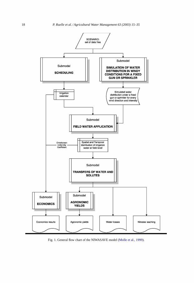
This integrated model is composed of four sub-models (seeFig. 1): scheduling, waterapplication, water and nitrate transfers and economics (Molle et al., 1999). The model canalso be used for solid set sprinklers or centre pivots for which spatial distribution of WADwas measured in windy conditions.


Fig. 1. General flow chart of the NIWASAVE model (Molle et al., 1999).


2.1.1. Sub-model for irrigation schedulingIt is used to establish the irrigation calendar on actual farming practices in the region.

The dates of water applications are calculated using a simplified water budget method,from an available climatic series. It can also take into account specific plot constraints(water or equipment availability, discharge limitations), and reflects climatic influence onmanagement decisions (rules to postpone irrigation for a few days in case of excessive rainor wind). The scheduling model is heavily dependent on local practices. It should thereforereflect specific regional practices.

2.1.2. Sub-models for simulating spatial distributions of water applicationThere is a sub-model for each irrigation technique: travelling rain gun machines, solid set

sprinklers and centre pivots. We only deal with the system involving rain gun machines. Themodel issemi-empiricaland uses six parameters that govern a conservative volume trans-formation of thereference no-windspatial distribution. The six parameters are wind-relatedand as previously mentioned they have been calibrated from field measurements. Threeparameters are used to describe jet behaviour, i.e. the wind drift in windy conditions. Ac-cording to the model ofRichards and Wetherhead (1993), wind speed, maximal range ofthe jet without wind, distance between a given point and the gun nozzle, are involved inthe wind drift calculation. The three others parameters allow the calculation of the rangeshortening while the jet is in motion due to cross-intrusion of wind (Augier, 1996). Therange shortening is calculated according to theRichards and Wetherhead equation (1993)in which the main jet trajectory direction versus horizontal plan and that of jet trajectoryversus wind direction are also used.

The spatial distribution of water at plot level is obtained by shifting and overlappingdistributions simulated under a single sprinkler or rain gun path for each day of irrigation.Wind speed and directions are obtained every 3 h from the local French meteorologicalservice records to take into account diurnal wind variations. In the case of gun sprinklers,both wind drift and evaporation losses are considered as negligible.

2.1.3. Sub-model for transfers of water and nitrates in the soil and crop yieldThe STICS model (Brisson et al., 1998) is used to simulate at a daily time step crop

development, water and nitrate budget in the soil. The water and nitrate transfer in the soilis based on the reservoir concept. Assuming the unit plot area is homogeneous, STICS cantake into account a maximum of five different soil layers, each one being characterised bythe following parameters: field capacity, welting point, bulk density and thickness. The cropparameter settings relative to corn, wheat, soybean, sunflower and linen are available; theparameters settingsfor others crops, especially for potatoes and sugarbeet aswell as forsome tropical crops are presently being established. Corn crop parameters are used here.

2.1.4. Sub-model for economics factorsThis sub-model (De Juan et al., 1996, 1999; Tarjuelo et al., 1996, 1999, 2000) has an eco-

nomic post processing function. It allows for the optimisation of the water quantity providedas a cost function of the different production factors (water, energy, seeds, fertilisers ) andtakes into account the environmental impact of irrigation. All the processing steps are car-ried out using the uniformity coefficients for each water application and crop yield. As little


interest has been shown in carrying out economical studies at the plot scale there is a scarcityof relevant economical assessment findings on environmental impacts. Consequently thissub-model is not used in our study, which focuses mainly on nitrate and water budgets.

2.1.5. Integration of sub-modelsThe different sub-models constituting the NIWASAVE model have been integrated within

a Windows environment. Output files provide the simulated spatial distributions year byyear, 40 variables are calculated including water, nitrates, yield components, and variousterms of water and nitrogen budgets. Complete simulations are made at every calculationpoint in the field. Each of them represents aplacetteof 5 m× 5 m (which can be modified)for irrigation with a travelling rain gun system. When the number of calculation points istoo high, a sampling procedure reduces them to a maximum of 250 points for which thetransfers of water and nitrates is simulated. Maps of water distribution and other variablesmay be displayed to analyse the spatial variability of the WAD. Yearly and inter-annualtemporal variability may also be investigated.

2.1.6. Application of the integrated model: definition of scenariosThe analysis of equipment configuration in a given context is performed using the sce-

narios. A scenario is defined from the description or the actual cropping practices includingirrigation, crop, soil and climate conditions, equipment selection and operational settingsin the field. Input files describe: (a) the meteorology: rainfall, potential ET, temperatureand global radiation recorded at daily rime steps, wind speed and direction recorded at3 h time steps; (b) the plot: dimensions and orientation; (c) the irrigation gun: trade mark,type, nozzle, pressure, jet angle, sector angle; parameters for spatial distribution simulation;(d) the crop, species and variety, precocity, temperature needs for reaching the successivevegetative stages, dates of cropping interventions (seedling, fertilisation, harvesting); (e)the soil nature, depth, soil parameters for various layers; (f) the irrigation calendar used (inconformity with local irrigation scheduling rules).

A scenario includes a large amount of detailed information, and produces after inte-grated model processing, a large quantity of data from which trends and conclusions canbe extracted. In this study the term “annual” will be used for a period of 12 months whichcorresponds with an agricultural campaign (from planting date of corn yearn until the daybefore planting next corn yearn + 1).

2.2. Scenarios

2.2.1. Reference scenarioThe reference scenario has been chosen to simulate objective farmer practices (an irriga-

tion schedule for a given yield target) with no water shortage and look at risks of N leachingon a shallow soil. It must be pointed out that such a scenario is closer to that of wet yearsthough the construction of a new dam will modify irrigation practices as water shortagesand irrigation bans will become a thing of the past.

General characteristics of the reference scenario:

(a) crop: corn (variety SAMSARA), cumulative temperature from sowing to maturity=1925◦ in basis 6◦, flowering temperature 1005◦ in basis 6◦;


Table 1Crop characteristics; corn (cv: Samsara)

Date of planting 20 AprilDate of harvest 10 OctoberPlanting depth (m) 0.03Maximum rooting depth (m) 1.20Maximum crop cover (%) 100Mulch cover at planting (%) 0Crop coefficient at full cover (kc) 1.20

(b) soil: shallow, calcareous, clayey soil which a rendzic leptosol (FAO-UNNESCO, 1989),local name: “groie sur banche plate”;

(c) irrigation machine: Nelson SR 100 travelling rain gun, 22 mm nozzle, 6 bar operatingpressure, 21◦ trajectory, 220◦ sector angle;

(d) four travel lanes of 250 m length, at 77 m spacing, oriented 340◦ from north;(e) travelling rain gun moving along a lane from north to south;(f) one lane watered per day during daytime;(g) irrigation calendar from typical irrigation rules for an intensive corn grower;(h) daily climate and hourly wind as recorded in Charente (southwest of France)

2.2.2. Crop and soil characteristicsThe crop and soil characteristics used in the NIWASAVE model are summarised in

Tables 1 and 2. The corn variety chosen (Samsara) is often sown in Charente region. Thesowing date is a representative one for the zone but this date varies from the 10th of April untilthe beginning of may depending on the climatic conditions of the year (temperature, rainand farmers constraints). The 10th of October have been chosen as the date for harvestingthough grain moisture is still high at this period during years with a rainy autumn, but thissimplification has little impact on soil water and nitrogen status.

Shallow soils are a general feature in the Charente basin but are also widespread in manyirrigated areas in south of France. The total available water capacity (AWC) for referencescenario soil is 48 mm, soil depth being around 40 cm (Table 2). This scenario providestypical data values for a field planted with corn on shallow soil.

2.2.3. Fertiliser applicationThe total fertiliser amount modelled was 220 kg N/ha, it is representative of application

levels commonly used by farmers on such a soil type and is close to levels recommendedfor irrigated corn by the extension services in the 1980s for an objective grain yield of11.5 t/ha (at standard humidity of 15%). It is divided into two applications: 45 kg/ha is spread

Table 2Layers and AWC of a typical shallow soil (calcareous clayey soil: rendzic leptosol) of Charente

Topsoil depth (m) 0.20Topsoil total AWC (mm m−1) 130Subsoil depth (m) 0.20Subsoil total AWC (mm m−1) 112


during the seedbed preparation, a few days before sowing and the 175 kg/ha remaining, isapplied at the beginning of June, at 8/10 leaf stage in the period when corn nitrogen needsincrease. The fertiliser applications used in the reference scenario are April 20 and June 10,respectively.

2.2.4. Climate dataWind speed (m/s) and direction (degrees from north) data, averaged over 3 h periods,

were obtained from Meteo-France for the weather station based in Cognac, for the periodof April–September, 1986–1996.

2.2.5. Irrigation schedulingThe irrigation schedule for corn was determined from studies of irrigation practices

at farm level in Charente (Labbe et al., 2000). The reference scenario used a simplifiedirrigation schedule at field scale. It is based on a water turn of 7 days and a irrigationinterruption period after rain of 1 day per 7 mm of rainfall depth with a threshold rainfalldepth value of 7 mm. It should be noted that maximum rainfall depth of 35 mm is takeninto account related to total AWC of the soil. The WAD D1 is 30 mm for each irrigationperiod.

Due to constraints at farm level that are not included in the schedule, the reference scenariomay overestimate the number of water applications but is representative of farmers whoirrigate without equipment constraints.

2.2.6. EquipmentThe gun is a Nelson SR 100 with a 22 mm nozzle, operated at 6 bar gun pressure with a 21◦

trajectory and a 220◦ sector angle. The gun moves along the lane at a speed of 16.7 m h−1

with a 38 m3 h−1 discharge. The reference field is composed of four lanes of 250 m length;one lane is irrigated per day in 15 h. Irrigation is carried out during the day, starting at5 h and stopping at 20 h. The lane spacing (77 m) is about 1.8 times the throw. This ratiois greater than typical recommendations of lane spacing for winds of 0–1 m s−1 but it isfrequently used with this type of gun. Of course, lane spacing used by farmers depend onfield width. Lane direction is 340◦ from north. Wind speed is frequently superior to 3 m s−1

during daytime and often oriented west due to the proximity of the ocean.

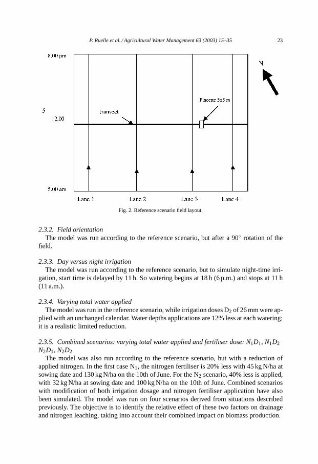
2.2.7. Spatial localisation of transectsThe field of the reference scenario is divided into transects (Fig. 2) which are split into

56 plots on a 5× 5 grid spacing. The reference transect is watered at midday. Each transectcrosses four lanes so each part of the reference transect is irrigated at the same time, i.e.12 a.m., on a different day over a 4 days period. Edge effects must be avoided in this studyto allow non-biased comparison of scenarios by NIWASAVE, so the field is limited to fourlanes.

2.3. Sub-scenarios

2.3.1. Variation in lane spacingThe simulations were performed according to the reference scenario, but another lane

spacing was used: 74 m. So, the lane length was reduced to maintain the same field surface.


Fig. 2. Reference scenario field layout.

2.3.2. Field orientationThe model was run according to the reference scenario, but after a 90◦ rotation of the

field.

2.3.3. Day versus night irrigationThe model was run according to the reference scenario, but to simulate night-time irri-

gation, start time is delayed by 11 h. So watering begins at 18 h (6 p.m.) and stops at 11 h(11 a.m.).

2.3.4. Varying total water appliedThe model was run in the reference scenario, while irrigation doses D2 of 26 mm were ap-

plied with an unchanged calendar. Water depths applications are 12% less at each watering;it is a realistic limited reduction.

2.3.5. Combined scenarios: varying total water applied and fertiliser dose: N1D1, N1D2N2D1, N2D2

The model was also run according to the reference scenario, but with a reduction ofapplied nitrogen. In the first case N1, the nitrogen fertiliser is 20% less with 45 kg N/ha atsowing date and 130 kg N/ha on the 10th of June. For the N2 scenario, 40% less is applied,with 32 kg N/ha at sowing date and 100 kg N/ha on the 10th of June. Combined scenarioswith modification of both irrigation dosage and nitrogen fertiliser application have alsobeen simulated. The model was run on four scenarios derived from situations describedpreviously. The objective is to identify the relative effect of these two factors on drainageand nitrogen leaching, taking into account their combined impact on biomass production.


2.4. Validation of the NIWASAVE model

Although the NIWASAVE model built and used in this study has not been validatedon the shallow soil context of the Charente on the basis of field experiments differentmodules have been independently calibrated and validated. The calibration and valida-tion of the water application module is described inMontero et al. (2001), Augier (1996)andRichards and Wetherhead (1993). The crop and transfer model (i.e. STICS) requiresreliable data but this information is always available. Nevertheless, one can cite recentworks (Brisson et al., 2002; Nemeth, 2001) attesting to a satisfactory confidence level re-garding the STICS simulations. Due to their respective independence, this should be asufficient guarantee attesting to the reliability of the NIWASAVE model. In addition ob-served field and simulated yield values can be compared for two available years (1995and 1996) within our study context: 10.5 versus 10.8 t/ha and 9.3 versus 9.2 t/ha, respec-tively. We do however recognise that this type of validation should be reinforced using fieldexperiments taking into account water and solute transfer on the shallow soil context ofCharente.

3. Results and discussion

The annual irrigation needs in Charente for the corn crop of the reference scenario wascalculated for a period of 30 years using a water balance model (Mailhol and Picheral,1994). Water requirements are theoretical values because this calculation does not take intoaccount any irrigation scheduling or WADs.Fig. 1shows that irrigation needs vary from 190to 360 mm during the 11-year interval that was used for NIWASAVE simulations. It appearsthat 1989 and 1990 are the driest years of the 30-year period and 1987 is the third wettest yearduring the same period (Fig. 2). The average irrigation needs for the 1986–1996 interval,used for NIWASAVE simulations, are 280 mm, value which is 8% higher than average for1960–1989.

3.1. Reference scenario

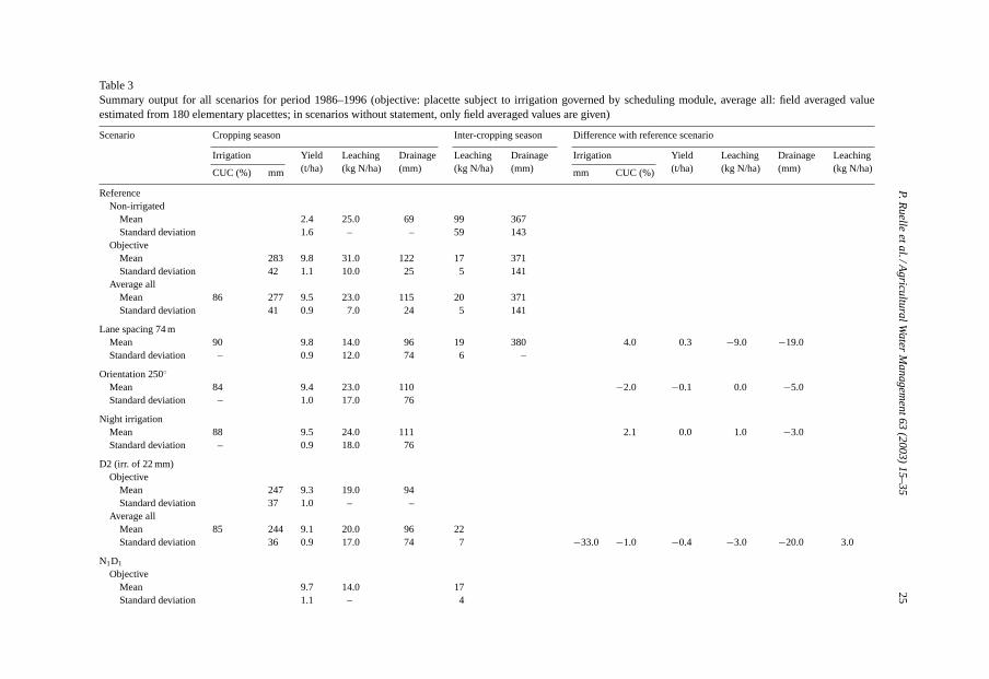
The NIWASAVE model was run on an 11-year period. Cumulative irrigation, drainageand N leaching values are computed for the cropping season from sowing date (20 April) toharvest date (10 October), and for the inter-cropping period. To compare variability at thefield scale, results are summarised inTable 3for mean and standard deviation calculated frommodel output on years 1986–1996. An averaged value is calculated from all 180 elementaryplots or “placettes” (an acceptable compromise between precision and computing time fora PC) simulated over the field. These 180 placettes are statistically representative of thedistribution function fitted by the WAD of the whole of the placettes. To analyse the results,three fictitious plots are simulated: a rain-fed placette an objective placette and a stress freeplacette. The rain-fed placette corresponds to a plot which does not receive any irrigation,the objective placette is subject to irrigation governed by the scheduling module (date, andWAD), the stress free placette corresponds to a plot without water and nitrogen limitationsand is used as a yield potentiality estimator (Fig. 3).

P.Ru

elle

eta

l./Ag

ricultu

ralW

ate

rM

an

agem

en

t63

(20

03

)1

5–

35

25Table 3Summary output for all scenarios for period 1986–1996 (objective: placette subject to irrigation governed by scheduling module, average all: field averaged valueestimated from 180 elementary placettes; in scenarios without statement, only field averaged values are given)

Scenario Cropping season Inter-cropping season Difference with reference scenario

Irrigation Yield(t/ha)

Leaching(kg N/ha)

Drainage(mm)

Leaching(kg N/ha)

Drainage(mm)


Leaching(kg N/ha)

Drainage(mm)

Leaching(kg N/ha)CUC (%) mm mm CUC (%)

ReferenceNon-irrigated

Mean 2.4 25.0 69 99 367Standard deviation 1.6 – – 59 143

ObjectiveMean 283 9.8 31.0 122 17 371Standard deviation 42 1.1 10.0 25 5 141

Average allMean 86 277 9.5 23.0 115 20 371Standard deviation 41 0.9 7.0 24 5 141

Lane spacing 74 mMean 90 9.8 14.0 96 19 380 4.0 0.3 −9.0 −19.0Standard deviation – 0.9 12.0 74 6 –

Orientation 250◦

Mean 84 9.4 23.0 110 −2.0 −0.1 0.0 −5.0Standard deviation – 1.0 17.0 76

Night irrigationMean 88 9.5 24.0 111 2.1 0.0 1.0 −3.0Standard deviation – 0.9 18.0 76

D2 (irr. of 22 mm)Objective

Mean 247 9.3 19.0 94Standard deviation 37 1.0 – –

Average allMean 85 244 9.1 20.0 96 22Standard deviation 36 0.9 17.0 74 7 −33.0 −1.0 −0.4 −3.0 −20.0 3.0

N1D1

ObjectiveMean 9.7 14.0 17Standard deviation 1.1 – 4

26P.R

ue

llee

tal./A

gricu

ltura

lWa

ter

Ma

nage

me

nt6

3(2

00

3)

15

–3

5

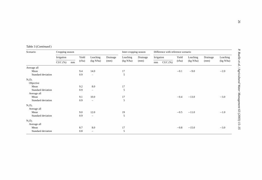
Table 3 (Continued)

Scenario Cropping season Inter-cropping season Difference with reference scenario


Leaching(kg N/ha)

Drainage(mm)

Leaching(kg N/ha)

Drainage(mm)


Leaching(kg N/ha)

Drainage(mm)

Leaching(kg N/ha)

CUC (%) mm mm CUC (%)

Average allMean 9.4 14.0 17 −0.1 −9.0 −2.0Standard deviation 0.9 – 5

N2D1

ObjectiveMean 9.2 8.0 17Standard deviation 0.9 – 5


N1D2


N2D2



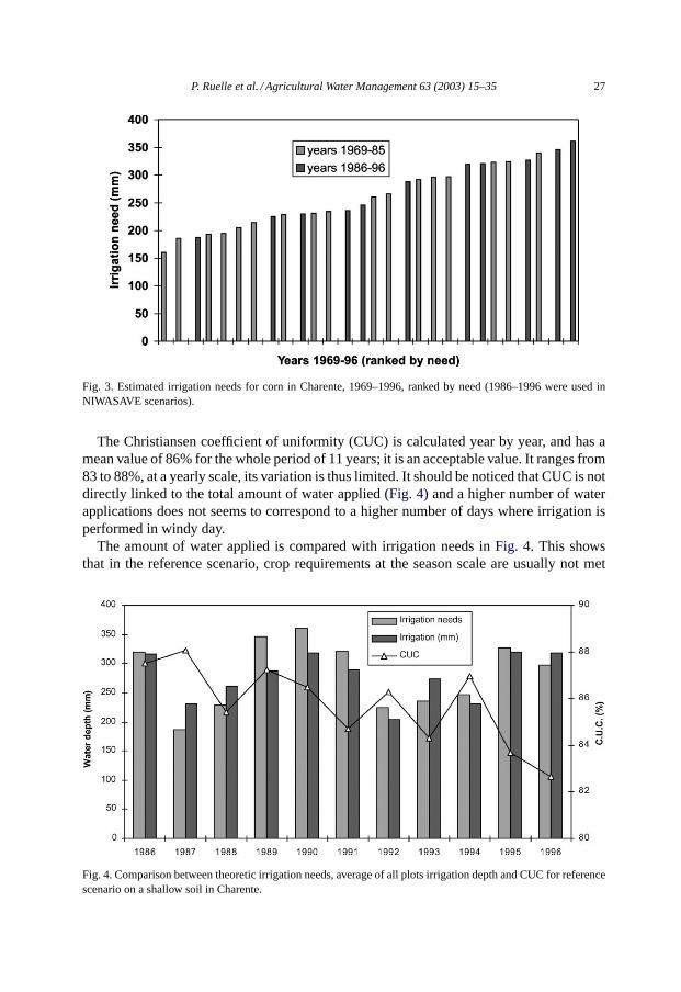
Fig. 3. Estimated irrigation needs for corn in Charente, 1969–1996, ranked by need (1986–1996 were used inNIWASAVE scenarios).

The Christiansen coefficient of uniformity (CUC) is calculated year by year, and has amean value of 86% for the whole period of 11 years; it is an acceptable value. It ranges from83 to 88%, at a yearly scale, its variation is thus limited. It should be noticed that CUC is notdirectly linked to the total amount of water applied (Fig. 4) and a higher number of waterapplications does not seems to correspond to a higher number of days where irrigation isperformed in windy day.

The amount of water applied is compared with irrigation needs inFig. 4. This showsthat in the reference scenario, crop requirements at the season scale are usually not met

Fig. 4. Comparison between theoretic irrigation needs, average of all plots irrigation depth and CUC for referencescenario on a shallow soil in Charente.


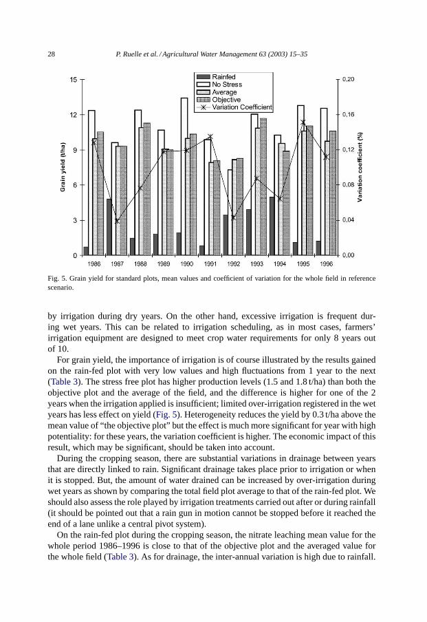
Fig. 5. Grain yield for standard plots, mean values and coefficient of variation for the whole field in referencescenario.

by irrigation during dry years. On the other hand, excessive irrigation is frequent dur-ing wet years. This can be related to irrigation scheduling, as in most cases, farmers’irrigation equipment are designed to meet crop water requirements for only 8 years outof 10.

For grain yield, the importance of irrigation is of course illustrated by the results gainedon the rain-fed plot with very low values and high fluctuations from 1 year to the next(Table 3). The stress free plot has higher production levels (1.5 and 1.8 t/ha) than both theobjective plot and the average of the field, and the difference is higher for one of the 2years when the irrigation applied is insufficient; limited over-irrigation registered in the wetyears has less effect on yield (Fig. 5). Heterogeneity reduces the yield by 0.3 t/ha above themean value of “the objective plot” but the effect is much more significant for year with highpotentiality: for these years, the variation coefficient is higher. The economic impact of thisresult, which may be significant, should be taken into account.

During the cropping season, there are substantial variations in drainage between yearsthat are directly linked to rain. Significant drainage takes place prior to irrigation or whenit is stopped. But, the amount of water drained can be increased by over-irrigation duringwet years as shown by comparing the total field plot average to that of the rain-fed plot. Weshould also assess the role played by irrigation treatments carried out after or during rainfall(it should be pointed out that a rain gun in motion cannot be stopped before it reached theend of a lane unlike a central pivot system).

On the rain-fed plot during the cropping season, the nitrate leaching mean value for thewhole period 1986–1996 is close to that of the objective plot and the averaged value forthe whole field (Table 3). As for drainage, the inter-annual variation is high due to rainfall.


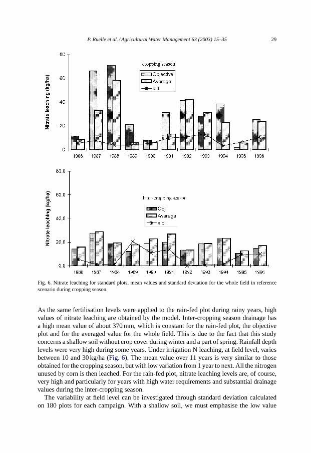
Fig. 6. Nitrate leaching for standard plots, mean values and standard deviation for the whole field in referencescenario during cropping season.

As the same fertilisation levels were applied to the rain-fed plot during rainy years, highvalues of nitrate leaching are obtained by the model. Inter-cropping season drainage hasa high mean value of about 370 mm, which is constant for the rain-fed plot, the objectiveplot and for the averaged value for the whole field. This is due to the fact that this studyconcerns a shallow soil without crop cover during winter and a part of spring. Rainfall depthlevels were very high during some years. Under irrigation N leaching, at field level, variesbetween 10 and 30 kg/ha (Fig. 6). The mean value over 11 years is very similar to thoseobtained for the cropping season, but with low variation from 1 year to next. All the nitrogenunused by corn is then leached. For the rain-fed plot, nitrate leaching levels are, of course,very high and particularly for years with high water requirements and substantial drainagevalues during the inter-cropping season.

The variability at field level can be investigated through standard deviation calculatedon 180 plots for each campaign. With a shallow soil, we must emphasise the low value


of water storage capacity so, standard deviation of drainage during inter-cropping seasonis negligible or null whatever the year considered. But to understand the variability ofnitrate leaching it is necessary to look at crop yield variability. The nitrate leaching standarddeviation is relatively lower when grain yield is low (e.g. 1987) and as is its converse (e.g.1990). We will analyse the case of two contrasting years.

In 1987, grain yield averaged on the whole field was equal to that of the “objective” plotand the nearby “stress free” plot with a low value of 9.3 t/ha. So, a substantial quantityof nitrate fertiliser was not used by the crop. Nitrate leaching occurred during croppingseason, with a high standard deviation. This was, as pointed out earlier, due to rainfall. Asnitrate leaching is higher on the objective plot, this can be linked to irrigation scheduling.The effects of irrigation on nitrate loss was less substantial over the whole field becausethe four lanes were irrigated on different days and as a consequence, the effect is evenedout.

As rainfall levels in 1990 were low during the irrigation season this affected the yields,10 t/ha for averaged field yield, 10.3 t/ha for the objective plot but the yield value was farhigher for the no stress placette. In such a situation, as in every dry year, the amount ofwater applied is insufficient to meet water requirements and the effect of heterogeneity onyield is higher. As a consequence, applied irrigation heterogeneity brought about increasedyield heterogeneity and inter-cropping season nitrate leaching.

Drainage and nitrate leaching have both a tendency to decrease from the first to thesubsequent travel lanes. This fact appears linked to the irrigation calendar and post rainwaiting rules. Analysis of the values calculated for the reference transect underlines theinter-annual variability of drainage and nitrate leaching during the cropping season and thesignificant differences between plots for certain years. However the results are smoothenedwhen the whole field is considered.

From the analysis of the reference scenario, it appears, as predicted, that in shallow soilsin Charente, when nitrogen fertilisation is in excess of crop needs, irrigation schedulingand specific water application levels have a role in nitrate leaching as does irrigation het-erogeneity. To prevent nitrate and water wastage, alternative scenarios are tested in the nextpart of the study.

Although the water requirements on the period 1986–1996 are not very significantlyhigher than those of 1969–1990, it would have been of course preferable to run the simu-lations over a longer period than the 11 years used here (wind data are only available from1986) to improve the confidence level of the results.

3.2. Equipment sub-scenario

3.2.1. Variation in lane spacingThe diminution of lane spacing induces a significant yield increase with a slight diminu-

tion in drainage and nitrate leaching. The variability along the transect is significantlylower than for the reference scenario. The lower yield values at the edges of the lanes in-side the field (in reference scenario) are eliminated. Drainage and nitrate leaching and theirinter-annual variability appear lower than those of reference scenario. A limited modifica-tion of lane spacing has a more significant effect on cases such as the one studied here. Thisis caused by the poor AWC of the a soil. However this result is obtained with a modification


of the width of the field and does not take into account edge effects occurring on a realfield.

3.2.2. Field orientationTable 3shows that output variables of the model are not significantly modified by rotating

the field of 90◦. The simulated values are similar to those of the reference scenario thoughthere is a slight diminution of CUC. In this region, wind direction is variable during summerand has only limited effects on irrigation; converse results were obtained in a valley with asingle wind direction like in the Rhone Valley (Molle et al., 1999).

3.2.3. Day versus night irrigationThere is usually less wind at night-time, but in the Charente, the comparison between

night-time and day-time irrigation does not reveal any effects on yield, drainage and nitrateleaching (Table 3).

3.2.4. Irrigation scheduling and fertilizer sub-scenario results3.2.4.1. Varying irrigation dose. Irrigation with smaller WAD levels reduces over-irrigation during wet years. With an irrigation dose D2 of 26 mm, the total amount of waterapplied during a dry year is similar to common practice in Charente when the scheduleand the number of irrigation treatments depends on irrigation bans imposed for most farms.Table 3summarises the results and comparisons with the reference scenario. The total fieldplot average for different outputs of the model remains close to the value obtained on theobjective plot.

Such a modification of irrigation depth induces a limited diminution of grain yield anddrainage but no significant reduction in nitrate leaching. Spatial irrigation and yield vari-ability have the same values as that of the reference scenario.

3.2.4.2. Varying fertiliser dose.A 20% reduction of the total amount of fertiliser appliedis tested in N1D1 and a 40% decrease is tested in N2D1 scenarios (Table 3). Once again, thereis no significant difference between results obtained on the objective plot and the average ofall plots. For the first scenario, the decrease of yield is only 0.1 t/ha. As expected the amountof nitrogen fertiliser applied was too high for the objective yield. In the second scenario, theyield losses reaches 0.4 t/ha and this value may require more detailed economic analysis toevaluate its impact on costs and revenue for farmers. We must note that N leaching decreasesbut is not completely eliminated.

3.2.4.3. Varying irrigation and fertiliser dosage.Similar results are obtained by a diminu-tion of WAD (N2D1) or a diminution of fertiliser levels (N1D2). A heavy decrease in Nleaching during the cropping season is thus obtained with the N2D2 scenario (Table 3),but as for the others scenarios N leaching remains at the same level during inter-croppingseason. Because of yield values, this alternative scenario may be of questionable interestfor farmers.

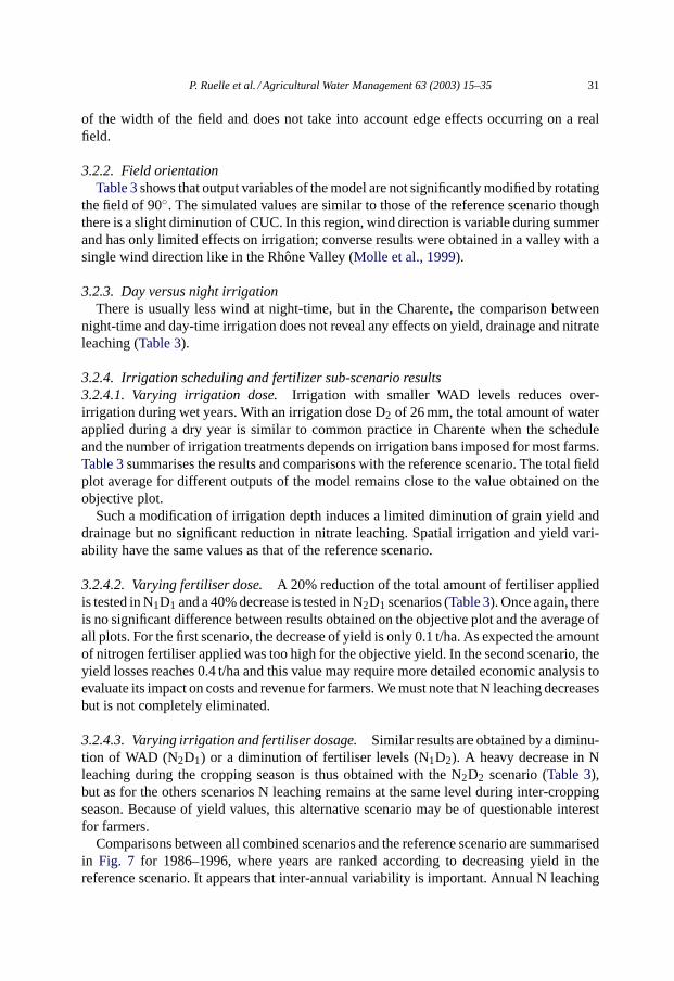
Comparisons between all combined scenarios and the reference scenario are summarisedin Fig. 7 for 1986–1996, where years are ranked according to decreasing yield in thereference scenario. It appears that inter-annual variability is important. Annual N leaching


Fig. 7. Comparison of yield and N leaching annual difference between combined scenarios and reference scenarios.The years are ranked for decreasing yield in reference scenario.

reduction with regard to the reference scenario is higher for higher nitrate losses (of thereference scenario) but it does not appear to be directly linked to yield reduction.

For a year such as 1988, with limited irrigation needs (Fig. 3), results of simulationssuggest that crop growth was affected by nitrogen stress brought on N leaching. On the


other hand, in 1992, yield losses are negligible and nitrate losses reduced in all alternativescenarios. In this case, irrigation needs and yield potential were low so a reduction of waterand/or N application induce a huge reduction of wastage levels. These examples illustratethat, after taking spatial variability inside a field into account, it is also necessary to rankfactors which contribute to drainage, N leaching and yield losses and to analyse the effectof a given scenario on climatic series.

4. Conclusion

In shallow soil for the scenarios analysed, changes in equipment used: field orientation (totake into account wind direction) and day versus night irrigation, have little effect on yieldand nitrate leaching. This may be related to the characteristics of the main winds (speed,direction and time-table versus irrigation time) for this region near Atlantic Ocean. But asexpected, lane spacing effects can be observed on yield and nitrate leaching. Significantresults are obtained on leaching and drainage by reducing both irrigation dosage and nitratefertiliser application levels.

In these specific climatic and shallow soil conditions, it must be pointed out that significantlevels of drainage are observed every year during the inter-cropping period whether the soilis irrigated or not. This phenomenon leads to a certain degree of nitrate leaching during thisperiod, so the reduction of leaching and drainage effects has to be dealt with as interactingmechanisms when their impacts on yield are discussed. Nitrate losses during the croppingseason are significant in comparison with those determined for deeper soils and also highlydependant on climatic conditions. So, to reach goals relating to environmental issues andsustainable agriculture, it is necessary to explore different ways of reducing environmentalimpacts and to develop tools to account for the effects of heterogeneity and interactionbetween different factors.

This study shows that fertiliser requirements are lower than the amount applied in thereference scenario. When simulating a 20% reduction in nitrogen fertiliser application levelsa very small 0.1 t/ha drop in yield (averaged value over 11 years) is registered. Use of shallowsoil levels for intensive production is a contentious issue and, as it mainly concerns wintercrops in France, a better determination of N requirements linked to potential campaign yieldis necessary.

To do so, the heterogeneity of the hydraulic properties of the soil has to be taken intoaccount, soil depth being certainly the main factor governing water and nitrogen fluxesbeneath root depth. Studies, such as ours, which deal with precision agriculture should usetools like the NIWASAVE model to account for the interaction of different factors linkedwith irrigation and fertiliser scheduling.

Acknowledgements

The study which lead to this paper is part of the NIWASAVE (FAIR, 1 CT950088; EUDG VI) programme supported by the European Union, the objective of which was to reducethe impact of water application heterogeneity on nitrate leaching water losses and economicyields.


References

Augier, P., 1996. Contribution à l’étude et à la modélisation mécaniste statistique de la distribution spatiale desapports d’eau sous un canon d’irrigation: Application à la caractérisation des effets du vent sur l’uniformitéd’arrosage. Thèse de doctorat de l’ENGREF, Montpellier, France.

Ben-Asher, J., Ayars, J.E., 1990. Deep seepage under non-uniform sprinkler irrigation. I. Theory. J. Irrig. Drain.Eng. 116 (3), 354–362.

Ben-Asher, J., Ayars, J.E., 1990. Deep seepage under non-uniform sprinkler irrigation. II. Field data. J. Irrig.Drain. Eng. 116 (3), 363–373.

Bresler, E., Dagan, G., 1988. Variability of yield of an irrigated crop and its causes. 1. Statement of the problemand methodology. Water Resour. Res. 24, 381–387.

Brisson, N., Seguin, B., Bertuzzi, P., 1992. Agrometeorological soil water balance for crop simulation models.Agric. Forest. Meteorol. 59, 267–287.

Brisson, N., Mary, B., Ripoche, D., Jeuffroy, M.H., Ruget, F., Nicoulaud, B., Gate, P., Devienne-Barret, F.,Antonioletti, R., Durr, C., Richard, G., Beaudoin, N., Recous, S., Tayot, X., Plenet, D., Cellier, P., Machet,J.M., Meynard, J., Delecolle, R., 1998. STICS: a generic model for the simulation of crops and their water andnitrogen balances. I. Theory and parameterization applied to wheat and corn. Agronomie 18, 311–346.

Brisson, N., Ruget, F., Gate, P., Lorgeou, J., Nicoullaud, B., Tayot, X., Plenet, D., Jeuffrroy, M.-H., Bouthier, A.,Ripoche, D., Mary, B., Justes, E., 2002. STICS: a generic model for the simulation of crops and their waterand nitrogen balances. II. Evaluation with comparison to actual experiment. Agronomie 22, 69–92.

Christiansen, J.E., 1942. Irrigation by sprinkling. University of California Berkeley Agriculture ExperimentalStation Bulletin, p. 670.

Cogels, O.G., 1983. An irrigation system uniformity function relating the effective uniformity of water applicationto the scale of influence of the plant root zones. Irrig. Sci. 4, 289–299.

Dagan, G., Bresler, E., 1988. Variability of yield of an irrigated crop and its causes. 3. Numerical simulation andfield results. Water Resour. Res. 24, 395–401.

De Juan, J.A., Tarjuelo, J.M., Valiente, M., Garcıa, P., 1996. Model for optimal cropping patterns within the farmbased on crop water production functions and irrigation uniformity. I: Development of a decision model. Agric.Water Manage. 1–2 (31), 115–143.

De Juan, J.A., Tarjuelo, J.M., Ortega, J.F., Valiente, M., Carrión, P., 1999. Management of water consumption inagriculture. A model for the economic optimisation of water use. Agric. Water Manage. 2–3 (40), 303–313.

FAO-UNNESCO, 1989. Carte mondiale des sols, légende révisée, rapport sur les ressources en sol du monde no60, 125 pp.

Kang, Y., Nishiyama, S., 1996. A simplified method for design of microirrigation laterals. Transactions of theASAE 39 (5), 1681–1687.

Kim, C.P., Stricker, J.N.M., 1996. Influence of spatially variable soil hydraulic properties and rainfall intensity onthe water budget. Water Resour. Res. 32 (6), 1699–1712.

Kincaid, D.C., 1996. Sprinkler pattern analysis for centre pivot irrigation. Irrig. Bus. Technol. 4 (4), 14–15.Labbe, F., Ruelle, P., Garin, P., Leroy, P., 2000. Modelling irrigation scheduling to analyse water management at

farm level, during water shortages. Eur. J. Agron. 12, 55–67.Leenhardt, D., Lafolie, F., Bruckler, L., 1998. Evaluating irrigation strategies for lettuce by simulation: 1. Water

flow simulations. Eur. J. Agron. 8, 249–265.Mailhol, J.C., Picheral, I., 1994. Regional water needs and crop yield according to water availability. In: Proceedings

of the 17th European Regional Conference on Irrigation and Drainage, May 16–22, 1994, vol. 2. ICID, Varna,pp. 73–82.

Mailhol, J.C., Ruelle, P., Nemeth, I., 2001. Impact of fertilisation practices on nitrogen leaching under irrigation.Irrig Sci. 20, 139–147.

Maraux, F., Lafolie, F., Bruckler, L., 1998. Comparison between mechanistic and functional models for estimatingsoil water balance: deterministic and stochastic approaches. Agric. Water Manage. 38, 1–20.

Mateos, L., Mantovani, E.C., Villalobos, F.J., 1997. Cotton response to non-uniformity of conventional sprinklerirrigation. Irrig. Sci. 17, 47–52.

Merriam, J.L., Keller, J., 1978. Farm Irrigation System Evaluation: A Guide for Management, 3rd ed. Utah StateUniversity, Logan.


Molle, B., Granier, J., Baudequin, D., Zanolin, A., 1999. Management of sprinkler irrigation spatial variability:consequences on crop yield, water amounts used and nitrates leaching. International Commission on Irrigationand Drainage (17 Congress), Granada, Spain, pp. 240–260.

Montero, J., Tajuello, J.M., Carrion, P., 2001. SIRIAS: a simulation model for sprinkler irrigation. II. Calibrationand validation of the model. Irrig. Sci. 20, 85–98.

Nemeth, I., 2001. Devenir de l’azote sous irrigation gravitaire. Application au cas d’un périmètre irrigué auMexique. Thèse de doctorat, Sciences de l’eau, Univ. Montpellier II, 216 p.

Normand, B., 1996. Etude expérimentale et modélisation du devenir de l’azote dans le système Eau-Sol-Planteatmosphère. Thèse de doctorat. Ph.D. Université Joseph Fournier, Grenoble, 190 pp.

Or, D., Hanks, R.J., 1992. Soil water and crop yield spatial variability induced by irrigation non-uniformity. SoilSci. Soc. Am. J. 56, 226–233.

Richards, P.J., Wetherhead, E.K., 1993. Prediction of rain gun patterns in windy conditions. J. Agric. Eng. Res.54 (4), 281–291.

Ruelle, P., 1995. Variabilité spatiale à l’échelle de parcelles de culture: étude expérimentale et modélisation desbilans hydriques et des rendements. Thèse mécanique. Univ. Joseph Fourier, Grenoble, 210 p.

Seginer, I., 1979. Irrigation uniformity related to horizontal extent of root zone. A computational study. Irrig. Sci.1, 89–96.

Solomon, K.H., 1984. Yield related interpretations of irrigation uniformity and efficiency measures. Irrig. Sci. 5,161–172.

Stern, J., Bresler, E., 1983. Nonuniform sprinkler irrigation and crop yield. Irrig. Sci. 4, 17–29.Tarjuelo, J.M., De Juan, J.A., Valiente, M., Garcıa, P., 1996. Model for optimal cropping patterns within the farm

based on crop water production functions and irrigation uniformity. II: A case study of irrigation schedulingin Albacete, Spain. Agric. Water Manage. 1–2 (31), 145–163.

Tarjuelo, J.M., Montero, J., Honrubia, F.T., Ortiz, J.J., Ortega, J.F., 1999. Analysis of uniformity of sprinkleirrigation in a semi-arid area. Agric. Water Manage. 2 (40), 315–331.

Tarjuelo, J.M., Ortega, J.F., Montero, J., De Juan, J.A., 2000. Modelling evaporation and drift losses in irrigationwith medium size impact sprinklers under semi-arid conditions. Agric. Water Manage. 3 (43), 263–284.

Warrick, A.W., Gardner, W.R., 1983. Crop yield as affected by spatial variations of soil and irrigation. WaterResour. Res. 19, 181–186.

Wilcox, J.C., Swailes, G.E., 1947. Uniformity of water distribution by some under-tree orchard sprinklers. Sci.Agric. 127, 565–583.

Using NIWASAVE to simulate impacts of irrigation heterogeneity on yield and nitrate leaching when...

Documents

Transcript of Using NIWASAVE to simulate impacts of irrigation heterogeneity on yield and nitrate leaching when...