1 The ever-changing world around usLand use is constantly changing. In urban areas new houses are being built at somelocations while older ones are being demolished elsewhere. Brownfield sites are beingimproved and industrial areas are reallocated outside city centres. Similar observationscan be made outside urban areas. Some farmers cultivate pieces of natural land andbuild new houses, while others abandon their plots, leaving them to renaturalize. Acrucial aspect these land-use changes have in common is that they are the result ofhuman decisions (Parker et al, 2008). These decisions are not made in isolation, butinstead influence each other. For example, people consider the availability of publicservices or transportation networks when choosing where to live. These facilities,however, are there because of earlier decisions on developments in the vicinity.

These examples illustrate the general notion that land use, both urban and rural,is a dynamic system. The land-use patterns one finds today are therefore essentially theresult of a series of previous and incremental land-use changes that affect each otherover time. These feedback mechanisms can cause developments that are initially smallto grow over time and reinforce each other (Arthur, 1999; Krugman, 1991), whichmakes the present land-use pattern highly path dependent (Brown et al, 2005).In order to explain and gain insights into land-use patterns it is therefore essential toconsider processes underlying these incremental changes.

For reasons of physical, economic, and ethical consideration we have only very limitedpossibilities to study land-use-change processes through experimentation (Janssen andOstrom, 2006). Therefore models seem to be the appropriate tools to gain insights intoland-use dynamics and we argue that these models should be able to generate land-usepatterns through decentralized local interactions, in line with Epstein's (1999) generativist'squestion.

An activity-based cellular automaton model to simulateland-use dynamics

Jasper van Vliet, Jelle Hurkens, Roger Whiteô, Hedwig van DeldenResearch Institute for Knowledge Systems, PO Box 463, 6200 AL Maastricht, The Netherlands;e-mail: Jvanvliet@riks.nl, Jhurkens@riks.nl, Roger@mun.nl, Hvdelden@riks.nlReceived 29 January 2009; in revised form 14 June 2010; published online 24 May 2011

Environment and Planning B: Planning and Design 2012, volume 39, pages 198 ^ 212

Abstract. In recent decades several methods have been proposed to simulate land-use changes ina spatially explicit way. In these models land is generally represented on a lattice with cell statesindicating the predominant land use. Since a cell can have only one state, mixed land uses anddifferent densities of one land use can only be introduced superficially, as separate cell states. Inthis paper we describe a cellular automata model that simulates dynamics in both land uses andactivities, where activities represent quantitative information, such as the number of inhabitants ata location. Therefore each cell has associated with it (1) a value representing one of a finite set ofland-use classes, and (2) a vector of numerical values representing the quantity of each modelledactivity that is present at that location. This allows simulation of incremental changes as well as mixedland uses. The proposed model is tested with a synthetic application that uses two activities:population and jobs. It simulates the emergence of human settlements over time from local inter-actions between activities and land uses. Assessment of results indicates that the model generatesrealistic urbanization patterns.

doi:10.1068/b36015

ôAlso of the Department of Geography, Memorial University of Newfoundland, St John's, A1B 3X9Canada.

In this paper we present an activity-based model, which can act as such a laboratoryfor land-use change. Section 2 gives an overview of land-use-modelling approachesin this direction. Section 3 then presents the activity-based model. Section 4 describesa case-study application that was used for assessment of this model and presents itsresults. Finally, section 5 discusses the results of the case study to draw conclusionsand give directions for future research.

2 Modelling land-use change2.1 Existing types of land-use modelsOver recent decades several approaches for modelling land use have been proposed.These approaches can be divided roughly into those originating from economics andthose originating from geography. Economists have been using approaches that aremostly founded on bid-rent curves as presented by Alonso (1964). These modelscompute an equilibrium situation, in which resulting land use or population densityis dependant on the distance to the urban centre, sometimes in combination with otherfactors (for an overview see Anas et al, 1998).

However useful these models are in the context of land pricing and urbanization,they have a few drawbacks that make them less suitable for the study of land-usedynamics. Time is not treated explicitly, and therefore developments over time, whichare elementary for some land-use dynamics, cannot be studied. Moreover, space isconsidered only as the distance to the urban centre, ignoring features that are nothomogeneous over space such as elevation, transport networks, or rivers. Followingfrom the introduction, we aim to understand land-use changes as an explicitly spatialand dynamic process. Therefore Alonso-type models are not considered further.

Geographers have focused on models that simulate land-use changes in an explicitlyspatial way, and hence developed models that can include spatially nonhomogeneousfactors such as elevation or transport networks. Overviews of different approaches areavailable in, among others,Veldkamp and Lambin (2001) and Koomen et al (2007). Fromthis group of models, we would like to consider two concepts for land-use-changemodelling in more detail: spatially explicit multiagent systems (MAS) and cellular autom-ata (CA)-based models. Because both approaches include time explicitly, they allow forfeedback mechanisms over time. Moreover, both methods approach human decisionmaking and generate land-use patterns from local dynamics (Brown et al, 2008; Whiteand Engelen, 2000).

In this discussion, agents in MAS are actors that can act and move independentlyover space. The advantage of MAS is that they can represent the behaviour of agents ina very straightforward way, since agents can interact directly with each other and withthe environment. More precisely, these local interactions between agents and differencesamong them generate the patterns observed on a global scale.

However, since the agents are the basic unit of computation, MAS are computa-tionally demanding. This is illustrated by an overview of case-study applications ofagent-based models for land-use-change modelling presented by Parker et al (2003). Inaddition, MAS require data at the level of actors, represented by agents, which makesthem data demanding and poses difficulties for model calibration and validation(Robinson et al, 2007). The problem of data collection is further thwarted by privacyregulations that are related to personal data.

CA, although sometimes also considered to be agent based, differ from MAS inthat sense that the basic unit for computation is a cell, not an agent. Together cellsmake up the lattice on which the CA exists, which makes them inherently spatial andtherefore very suitable for the simulation of land-use dynamics. Since the cell is thebasic unit of computation and cell sizes can be adjusted according to the scope of

An activity-based cellular automaton model to simulate land-use dynamics 199

application, models can keep a computational efficiency. Therefore, CA have beenapplied to simulate land-use changes on larger scales, from urban areas (for example,Van Vliet et al, 2009) to groups of countries (eg Van Delden et al, 2010). Simulatingland-use changes at a rather high level of abstraction brings the advantage that CAare less data demanding compared with MAS. Although calibration and validationof these models has been considered a major issue, numerous calibrated examples areavailable (Hagen-Zanker and Lajoie, 2008; Van Vliet et al, 2009; Wickramasuriya et al,2009).

The advantages of CA come at the cost of detail: individual actors are not consid-ered. Instead cells have a state, which generally represents the predominant land use.However, a cell can have only one land use, and land uses are thus by definitionmutually exclusive. Therefore combinations of land uses are not possible at one loca-tion unless it is explicitly defined as a separate mixed class. Still, in reality mixed landuse is the rule rather than the exception. Hence CA cannot represent the richness anddiversity in land uses one observes in reality.

2.2 Bridging the gap between MAS and CASeveral efforts have been made to fill the gap between CA and MAS by addingquantitative information to CA-based land-use models. In regional applications oftheir constrained CA model, White and Engelen (1997) first compute for each regiona density to translate the number of inhabitants or jobs in a cell to the demand for theassociated residential or commercial land uses. Consequently, cells in their model havea density, but this density is similar in all locations with the same land use within oneregion. Hence, their model simulates regional differences but not local ones.

Loibl and To« tzer (2003) follow a similar approach to model migration at a regionallevel. However, their model adds more detail at the local level, as households andenterprises are allocated on the lattice on the basis of local characteristics. Therefore,densities can vary cell by cell and urban growth is simulated as an incremental process.

Wu (1998) simulates urbanization by explicitly allocating residents on a lattice,which allows for incremental changes in population density. As such he is able tosimulate both monocentric and polycentric urban land-use patterns, depending onthe regimes used for allocation. Wu and Webster (1998; 2000) elaborate on the alloca-tion of land development as they combine a CA approach with multicriteria evaluationand neoclassical urban economic theories. In their model land development increasesincrementally, according to the profitability of the development of a location. This isagain a function of the development in the neighbourhood of that location.

Yeh and Li (2002) also acknowledge that densities of urban areas differ consider-ably from one city to another and for different locations within one city. Theirapproach differs from Wu (1998) and Wu and Webster (1998; 2000) in that land usesare considered separately from population densities. They model development densityproportional to the development probability as computed from the CA transition rules.The CA model then assigns a density to those locations that change from undevelopedland into urban land. Depending on the parameters in the transition rules, the modelcan simulate different urbanization patterns, both monocentric and polycentric. More-over the cells that are not urban can have a `grey value' between 0 and 1 that indicateshow far a particular location is from urbanization.

From these examples it becomes clear that the addition of activity or informationon density has been studied before in a dynamic and spatial environment, using severaldifferent approaches. Similar to Wu (1998),Wu and Webster (1998; 2002), and Yeh andLi (2002) we see activity density as a cell property, which changes in small butincremental steps. In addition, like Yeh and Li (2002), we account for activities in a

200 J van Vliet, J Hurkens, R White, H van Delden

separate data layer. However, these models have in common that they focus on urbanland-use change and particularly on growth. Typically, densities are changing incre-mentally, but changes are one-directional towards urbanization or an increase indevelopment. Consequently, nonurban land uses are background; they can influencethe allocation of population or urban densification, but they do not change them-selves as a result thereof, except when they change into urban land. In addition mixedland uses or multifunctional land uses only exist superficially as cells that are not fullyurbanized. This does not reflect the richness that exists in reality, such as locations witha combination of commercial and residential uses. Hence these approaches poseproblems for the simulation of inner-city dynamics or rural depopulation.

The model presented in this paper adds to the CA framework the notion of activities,where activities represent the general idea of a density. For example, population can bethe activity related to residential land use, and jobs can be the activity associated withindustrial land use. Because a location can have more than one activity, mixed landuses can be represented explicitly as more than one activity at the same location, notnecessarily related to the predominant land use. As the amount of activity at a locationcan increase as well as decrease, the proposed model allows for the study of a range ofland-use-change processes, from urban growth to rural depopulation.

As the cell remains the basic unit of computation, this model is an extensionof the existing computational framework of CA land-use models. Because activityis considered as a cell property rather than a set of agents it is not considered to bea MAS.

3 The activity-based model3.1 The Metronamica land-use modelling frameworkCA land-use models generally exist on a lattice of regular squares. Each cell on thelattice has one of a limited number of cell states which represents the predominant landuse at that location. In each discrete time step, cell states are updated simultaneouslyaccording to a set of transition rules. The characteristic of CA models is that the stateof adjacent cells, and hence the land use in the neighbourhood of a location, is input tothe transition rules. Additional factors are often added to represent heterogeneousgeographic features. The activity-based approach is founded on the CA model aspresented by White et al (1997) and further developed as the Metronamica land-usemodelling framework (RIKS, 2009). Metronamica uses three land-use types: constrainedland uses, which are actively allocated by the CA; features, which are not supposed tochange during a simulation; and unconstrained land uses, which only change as aresult of other changes. `Constrained' refers to the notion that the total number of cellsper land-use type is determined exogenously (White et al, 1997). In land-use terms,the total area demand for a constrained land use in a certain time step is definedexternally, while this demand is then allocated by the CA. Land-use allocation is drivenby the potential of cells, an endogenous variable that is calculated for every locationand each constrained land-use class:

Pt�1g, i � Nt�1

g, i St�1g, i Z

t�1g, i A

t�1g, i v ,

where, for land use g on cell i, Pg, i is the transition potential, Ng, i is the neighbourhoodeffect, Sg i is the physical suitability, Zg, i is the zoning status, Ag, i is the accessibility,and v is a stochastic perturbation term. The latter is added to represent the differentpreferences that individual actors have and to account for variation in factors that arenot otherwise represented. Time-dependent variables are indicated with superscripts,where t indicates that information is taken from the existing situation, and t� 1indicates that this information is used for land-use allocation in the next time step.

An activity-based cellular automaton model to simulate land-use dynamics 201

Factors that represent physical suitability, zoning, and accessibility can have valuesbetween 0 and 1.

The neighbourhood effect is the dynamic component of the CA algorithm whichaccounts for the self-organizing behaviour of the model. It is calculated from the landuses in the neighbourhood of a location:

Nt�1g; i �

Xj

wd�i; j �; g; l t� j � ,

where wd; g; l is the neighbourhood rule that describes the effect of land use l at locationj and distance d(i, j) on the potential of location i for land use g. This land use is takenfrom the previous time step.

Constrained land uses are allocated to those cells that have the highest transitionpotential until the demands are fulfilled. Locations that do not have a feature ofconstrained land use will be given the unconstrained land use for which they havethe highest suitability.

3.2 Adding activities to the Metronamica frameworkIn the original Metronamica modelling framework, land uses are constrained by anarea demand. However, in reality many land uses are not constrained by an area, butrather by an amount of activity. In the case of urban expansion it is not an amountof land surface that needs to be covered by urban fabric, but the population that needsa place to live. Therefore, in the activity-based approach, the total demand is notconstrained in terms of cells, but in terms of activity instead. Hence, for each timestep the amount of activity that needs to be allocated on the lattice is defined exoge-nously. After the activity allocation, land uses that are associated with activities areassigned on the basis of the new activity distribution. The number of cells per land usethus depends on the density of the activity. A high density requires fewer cells than alower density.

Additionally, the land uses in the area surrounding a location are input to theneighbourhood effect in the original constrained CA. For example commercial areasin the vicinity make a location more attractive for residential development as theyrepresent jobs and services. As quantitative information is available in the activity-based model, it is now possible to define the attraction as a function of the number ofjobs rather than just the presence of commercial land use. Hence, locations that havea high job density in their commercial areas are more attractive to residents thanlocations with only a low density. At the same time, the compatibility of the existingland use will influence the amount of activity that can be allocated to a cell.

Since not all land uses can be associated with an activity, we have four typesof land uses in our model. These are activity-constrained land uses, area-constrainedland uses, features, and unconstrained land uses. Hence the activity-constrained landuses are added to the existing Metronamica framework. Features do not change,activity-constrained land uses are assigned on the basis of their activity distribution,area constrained land uses are allocated after that, and finally, all cells that are notassigned a feature or one of the constrained land uses are allocated an unconstrainedland use. The order of allocation of land-use types represents the economic influenceor power that is associated with these land uses.

An obvious example of an activity-constrained land use is residential land use, withpopulation as the associated activity. It should be noted that each activity-constrainedland use has only one associated activity. An example of an area-constrained land useis agriculture, for which the demand is expressed as a number of cells. Unconstrainedland uses are often natural land uses, which occupy all locations that are not occu-pied by land uses which are driven by an external demand. Similar to the original

202 J van Vliet, J Hurkens, R White, H van Delden

Metronamica framework, the model requires at least one unconstrained land-use classto make sure that all cells will have a land use at any time.

To keep track of activities, an additional data layer is required for each type ofactivity. Hence a cell no longer has only one discrete cell state. Instead it has a land-usestate, and one numerical value for each activity. Computation of land-use dynamicstherefore becomes a two-step process, as presented in figure 1. In each time step, firstthe demand for activities (a) is distributed according to the potential of each locationfor that activity (b). This potential for each activity is a function of the land-use andactivity distribution in the previous time step [(c) and (d), respectively], as well as thesuitability, zoning status, and accessibility of that location (e). Activity-constrained landuses are then assigned on the basis of the updated activity distribution (f ). Similarly,the total potential for area-constrained land uses is computed on the basis of the land-use and activity distribution from the previous time step [(g) and (h), respectively] andthe suitability, zoning status, and accessibility of that location (i). These land uses areallocated accordingly ( j) until the area demand (k) is fulfilled.

An important characteristic of the proposed activity-based model is that it is ageneric model that aims to simulate urbanization from the bottom up. According tourban economic theory, urbanization is the result of the interplay between centripetaland centrifugal forces (Furtado et al, submitted; Krugman, 1996). The activity-basedmodel incorporates both forces. Agglomeration effects are simulated by the mutualattraction of activities creating economies of scale. However, this agglomeration advan-tage will generate competition for space, which leads to higher land prices, congestion,and pollution that are associated with higher activity densities. These diseconomies ofscale cause centrifugal forces. Both forces are included in the proposed activity-basedmodel details of which are provided in the next section.

Activitydemand Area demand

Geographical aspects (suitability,zoning, accessibility)

Activitypotential

Land-usepotential

Activitydistribution

Land-use map

(a) (e) (i) (k)

(b)

(d) (c) (g) (h)

(j)

(f)

Figure 1. System diagram for land-use and activity distribution. Arrows show the flow ofinformation, solid lines represent current values, and dashed lines represent values from theprevious time step. Other symbols are explained in the text.

An activity-based cellular automaton model to simulate land-use dynamics 203

3.3 Activity distribution and land-use allocationActivity is distributed proportionally according to a cell's potential for this activity,which is computed according to the following equation:

P t�1k; i � ck; i �gt�fÿNt�1

k; i � Et�1k; i � e

�St�1k; i Z

t�1k; i A

t�1k; i ,

where, for activity k in cell i, Pk; i is the potential, ck; i �g) is the compatibility coefficientthat indicates how well the activity can be accommodated by existing land use g, f(x)is a transformation function to avoid negative potentials, f(x)� ln (1� 2x ), Nk; i is theneighbourhood effect, Ek; i is the diseconomies of scale effect, e is a scalable stochasticvariable drawn from a normal (0, a) distribution, Sk; i is a factor that represents thephysical suitability, Zk; i is a factor that represents the zoning status, and Ak; i is a factorthat represents the accessibility to transport networks. Time-dependent variables areindicated with superscripts, where t indicates that information is taken from theexisting situation, and t� 1 indicates that this information is used for activityallocation in the next time step. The factors that represent physical suitability, zoning,and accessibility have values between 0 and 1. The stochastic variable is drawnindependently for each cell and in each time step, and its effect is scalable withparameter a.

The neighbourhood effect Nk; i is a function of the existing activity distribution inthe neighbourhood of a cell. It is computed as the sum of the effects of all cells j at alldistances d in the neighbourhood. This includes the activity and the land use of cell iitself.

Nt�1k; i �

Xj

wd�i; j �; k; h� j �Xth�j� ,

where wd;k;h is the weight function representing the attraction or repulsion of activity hon activity k at location j and distance d, and Xt

h� j � is the amount of activity h in cell j.The activity of area-constrained land uses and unconstrained land uses follow theKronecker delta function: they are 1 wherever land use is present, and 0 in all othercells. Diseconomies of scale represent the negative effects of agglomeration. This effectis computed as a function of the neighbourhood effect for that activity for a specificlocation:

Et�1k; i � g1

ÿNt�1

k; i

�g2 ,where g1 and g2 are parameters that need to be calibrated. Typically, ÿ1 < g1 < 0 andg2 > 1 to make sure that negative externalities are small initially and grow more thanproportionally with the present activity.

Once the activity potentials are calculated for all cells j, the amount of activity kthat is assigned to a particular cell i, Xk; i , is proportional to the activity potential of thatcell:

Xt�1k; i �

Pt�1k; iX

j

P t�1k; j

.

Once the amount of each activity in each cell is known, the associated land uses areassigned to those cells that have an activity higher than a predefined threshold value.When more than one activity exceeds this threshold value, the cell is assigned the landuse for which the activity is highest relative to the threshold value. The threshold valuescan differ for the different types of activity. Regardless of the assigned land use, all cellsmaintain their activities.

To allocate area-constrained land uses, the potential for these land uses is com-puted for each cell and for each area-constrained land use. Note that similarly to the

204 J van Vliet, J Hurkens, R White, H van Delden

potential for activities, this potential is computed on the basis of the activity distributionfrom the previous time step. Since area-constrained land uses are not represented witha quantity, there are also no diseconomies of scale:

Pt�1g; i � f

ÿNt�1

g; i � e�St�1g; i Z

t�1g; i A

t�1g; i ,

where, for land use g and cell i, Pg; i is the total potential, and Ng; i is the neighbourhoodeffect. The neighbourhood effect for area-constrained land uses is computed exactlysimilarly to the neighbourhood effect for activities. This differs from the originalMetronamica in that the neighbourhood effect is a function of the activity distributionrather than the land-use pattern.

Area-constrained land uses are assigned to cells with the highest potential until thedemand for this land use is met and as long as these cells are not already occupiedby an activity-constrained land-use state. Finally, all cells that are not occupied byeither an activity-constrained land use or an area-constrained land use receive anunconstrained land use.

4 A synthetic case study4.1 The case-study applicationA synthetic application is used to test the hypothesis that settlement patterns cangrow from local interactions between activities and land uses. Hence the case studydoes not include geographical information such as physical suitability, spatial plan-ning, or accessibility to transport networks. The case study is defined on a regularlattice of 2006200 cells, which for illustrative purposes can be taken to represent1 ha each. Thus the total area comprises 40 000 cells or 400 km2. The application isused to simulate land-use change over a period of 1000 time steps that represent oneyear each.

The case-study application has two activity-constrained land-use types. These areresidential land and industrial land, and associated with these are the activitiespopulation and jobs, respectively. An initial small amount of population and jobswas distributed randomly over the area. Over time, population increased linearlyfrom approximately 600 at t � 0 to 60 000 at t � 1000, while the number of jobsincreased linearly from approximately 300 at t � 0 to 30 000 at t � 1000. As well asresidential land and industrial land, there is one area-constrained land use, which isagricultural land. We assumed that 1 ha is sufficient to feed 10 persons, therefore thearea demand for agriculture increases from 1 cell at t � 0 to 6000 cells at t � 1000.Finally, there is one unconstrained land use, which is natural land. All cells thatare not occupied by residential, industrial, or agricultural land become natural land.The case-study application does not contain any features.

To evaluate the activity-based model we consider the land-use patterns that aregenerated at t � 1000, which is assessed visually and by the statistical signature(Moss, 2002). Additionally the meaning of the parameters in the transition rules aswell as the path towards the eventual land-use pattern are evaluated.

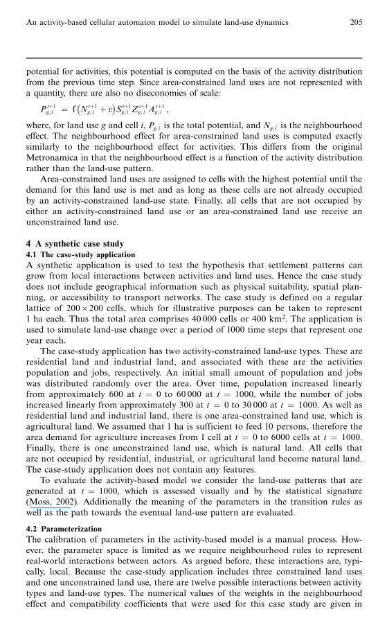
4.2 ParameterizationThe calibration of parameters in the activity-based model is a manual process. How-ever, the parameter space is limited as we require neighbourhood rules to representreal-world interactions between actors. As argued before, these interactions are, typi-cally, local. Because the case-study application includes three constrained land usesand one unconstrained land use, there are twelve possible interactions between activitytypes and land-use types. The numerical values of the weights in the neighbourhoodeffect and compatibility coefficients that were used for this case study are given in

An activity-based cellular automaton model to simulate land-use dynamics 205

table 1 and table 2, respectively. It should be noted that weights that represent the effectof population and jobs are low relative to the effect of other activities. This is becausethe weights are multiplied by the respective activities at a location. The density forpopulation and jobs is typically much higher than the activity density of 1 associatedwith agricultural and natural land.

Population, associated with residential land, can be allocated on all land-use types,but has a natural preference for residential land uses, represented in its compatibilityfactor. Population is attracted by existing population in the same location as well as inthe direct vicinity. This represents the social interactions or the availability of generalfacilities implied by the clustering of a larger number of people. Jobs and agricultureattract population at a small distance, representing employment and the availabilityof food in the neighbourhood.

Jobs show behaviour similar to population. They can be allocated on all land uses,although natural land is by far the least attractive, as represented by the relatively lowcompatibility coefficient. Both agriculture and jobs attract jobs in their vicinity, sinceboth represent employment. Clustering creates additional employment, for the process-ing of products, and benefits of scale such as those described by, among others, Arthur(1990). Jobs are attracted by population, because people represent both customers andemployees.

Agricultural land is attracted by areas where there is population, because popula-tion represents farmers to work the fields and customers for their products andtherefore a lower distance to markets. The latter also explains why an accumulationof population is more attractive for agricultural land than a mere presence of it.A similar relation, but much less strong, exists between jobs and agriculturebecause jobs indicate a processing industry. Natural land is not of any influence on

Table 1. Weights of the neighbourhood effect as used in the case-study application. Weights areinterpolated linearly between the indicated values.

Activity interactions Distance (cells)

0 1 2 3 4

From population to population 30 0.25 0.001 0 0From population to jobs 0.1 0.4 0 0 0From population to agriculture 0 3 0.5 0.25 0From jobs to population 0 0.5 0 0 0From jobs to jobs 20 0.45 0 0 0From jobs to agriculture 0 2 0 0 0From agriculture to population 4 1.5 0.2 0.1 0From agriculture to jobs 0 2 0 0 0From agriculture to agriculture 300 5 0 0 0From nature to population 0 0 0 0 0From nature to jobs 0 0 0 0 0From nature to agriculture 0 0 0 0 0

Table 2. Compatibility coefficients as used in the case-study application.

Land use Compatibility Compatibilitywith population with jobs

Natural 0.6 0.5Residential 1.0 0.7Industrial 0.4 1.0Agricultural 0.7 0.7

206 J van Vliet, J Hurkens, R White, H van Delden

agriculture since it does not represent any apparent attraction or repulsion. Naturalland itself is not allocated according to transition rules, since it only occupieslocations that are not already residential, industrial, or agricultural land. Thereforethere is no interaction effect from other land uses or activities on land defined asnatural.

4.3 Simulation resultsFigure 2 shows snapshots of the land use, the population distribution, and the jobdistribution at regular intervals in time. Maps are taken from one single run, butbecause all simulation runs show similar results, it is taken as a representative example.The maps show that initially activities are distributed more or less randomly overspace, as are the plots of agricultural land. Activity is not yet clustered to the extentthat any residential or industrial land appears. As time progresses and the amount ofactivity increases, activity clusters and so does the agricultural land. The first smallpatches of residential land appear in the centre of larger agricultural areas, andcontinue to grow as the population increases. Eventually, some urban clusters growbigger over time, while most of them remain small. As jobs cluster in locations with aconcentration of population, locations with industrial land appear at the edge of largerurban clusters, while some others are more isolated.

The emergence of the settlement pattern over time occurs in several stages, whichare associated with an increasingly more-developed economy. Initially people clustertogether only a little in agricultural areas, representing the development of the primarysector. Then as the population grows the first settlements appear which equates to thesecondary sector as some form of organization is required. Most settlements staysmall, while some grow over time to become more central cities. It is mostly aroundthese larger cities that jobs cluster, to the extent that industrial land use appearsindicating a developing tertiary sector.

4.4 Urban cluster distributionThe described settlement pattern emerges from strictly local interactions betweenactivities. These incremental activity changes eventually exhibit themselves as land-usechanges, in accordance with the initial hypothesis. However, as a description is onlysubjective, the generated land-use patterns and activity distribution are also assessedobjectively.

Models for land-use change are often evaluated by their capability to simulateaccurately historical land-use changes (Pontius et al, 2008), where accuracy is assessed,typically, on a pixel level using map comparison techniques (Hagen, 2002; Pontiuset al, 2004). Since the aim of this study is to test the ability to generate realisticurbanization patterns rather than to simulate changes accurately, we use a syntheticapplication and therefore we have no historic land-use changes for comparison.

For reasonably large areas the distribution of urban cluster sizes is known to followZipf's law, also known as the rank ^ size rule (Cordoba, 2008; Gabaix, 1999; Krugman,1996; Reed, 2002). For this, clusters of direct adjacent residential and industrial landare ranked, where rank 1 represents the largest cluster, 2 the next largest, and so on.Cluster sizes are measured from the population in that cluster in the simulation resultsat t � 1000. The rank ^ size rule indicates that this distribution approximates a powerlaw as follows:

size � a6rankb .

Figure 3 shows this rank ^ size distribution for one simulation result, including thepower law that best approximates this distribution.

An activity-based cellular automaton model to simulate land-use dynamics 207

208Jvan

Vliet,

JHurkens,

RW

hite,H

vanDelden

N:/psfiles/epb3902w

/

t � 200 t � 400 t � 600 t � 800 t � 1000

Land use

Natural

Residential

Industrial

Agricultural

Population per cell

45.8 ± 100.0

20.7 ± 45.8

9.1 ± 20.7

3.7 ± 9.1

1.2 ± 3.7

0 ± 1.2

Jobs per cell

10.4 ± 20.0

5.2 ± 10.4

2.4 ± 5.2

0.8 ± 2.4

0 ± 0.8

Figure 2. [In colour online.] Time series representing land-use and activity distributions of a typical simulation run for regular intervals in time.

As described in section 3, to generate realistic patterns the model includes somenoise, represented with a normally distributed random variable. Therefore it is notsufficient to assess only one simulation result as this could be an outlier. Hence themodel was run several times starting with a different random seed and results wereassessed. Results for ten simulation results are presented in table 3.

The R 2-values that are close to 1 indicate that the land-use patterns that aregenerated closely follow the expected rank ^ size rule. Moreover, the slope of the powerlaw function that describes the cluster-size distribution is close to the value if ÿ1 aswas expected from the literature (Cordoba, 2008; Gabaix, 1999). This shows that theactivity-based CA can generate realistic land-use settlement patterns.

The exact shape of this power law is a function of two forces, the neighbourhoodeffect working as a centripetal force with the diseconomies of scale and the stochasticperturbation working as centrifugal forces. Adjustments to the size of both forcesalso adjusts the rank ^ size distribution, with a tendency towards several large settle-ments or more numerous small ones depending on the exact parameterization. Inthe extreme case, without centrifugal forces, the model generates the von Thu« nensolution with one large residential area surrounded by agricultural land in the middleof a natural area.

10 000

1000

100

10

1

Cluster

size

y � 1854:5xÿ1:0669

R 2 � 0:9902

1 10 100Rank

Figure 3. Cluster-size distribution for the result of one typical simulation run at time t � 1000.

Table 3. Generated urban settlement structures, expressed as estimated parameters for the powerlaw that best describes their rank ^ size distribution. See text for further explanation.

Simulation a b R 2

1 1937 ÿ1.02 0.972 2422 ÿ1.12 0.973 1614 ÿ0.99 0.984 2204 ÿ1.10 0.975 1855 ÿ1.07 0.996 1642 ÿ1.01 0.977 1916 ÿ1.03 0.998 2071 ÿ1.14 0.979 2048 ÿ1.18 0.9610 2286 ÿ1.16 0.97

An activity-based cellular automaton model to simulate land-use dynamics 209

5 Conclusions and directions for further researchUsing activities to simulate land-use dynamics combines aspects of CA and MASland-use models: the cell is still the basic unit of computation, but this is comple-mented with information and behaviour of actors as represented by activities. Thisapproach adds to the constrained CA framework in three ways. Firstly, the presenceof activity gives more information than merely the land-use states, which are rathersuperficial. The model explicitly allows mixed land uses as well as a variation indensities for activities for each cell, from sparse residential areas to densely populatedlocations. Secondly, land-use dynamics are the result of many smaller and incrementalchanges rather than a sudden change in cell states. Thirdly, the activity-based modelexplicitly allows the inclusion of feedback between activities and hence represents theprocess of land-use change in more detail.

Assessment of the behaviour and results shows that the activity-based modelgenerates realistic land-use patterns. As the inclusion of activities allows the repre-sentation of land-use-change processes more accurately, we expect that this approachwill improve the results of real-world applications for land-use modelling. This isparticularly the case for processes such as rural depopulation or urban sprawl thatare the result of incremental changes in activity location rather than sudden changesin the land use.

Therefore the obvious next step is to test the activity-based CA model for itsability to mimic historical changes in land use and activities accurately. For thisthe activity-based model should include real-world aspects, represented by physicalsuitability, zoning maps, and transport networks. A first attempt shows promisingresults in that direction (Van Vliet and Van Delden, 2008) but requires more exten-sive testing on aspects such as robustness and scale sensitivity such as that alreadydone for other CA models (Kocabas and Dragicevic, 2006; Menard and Marceau,2005).

An advantage of the activity-based approach over MAS is that the data demand isrelatively low. To calibrate an application for historical changes, land-use data as wellas data for activities such as population and jobs are required for at least two points intime. For independent validation another dataset for a third point in time is required.Due to developments in remote sensing, land-use data are currently easily available.For population data or other activities this is not yet the case. However, severalapproaches have been developed to estimate population density at the level of cellsby using satellite imagery (Harvey, 2002; Wu and Murray, 2007) or from land-use maps(Gallego and Peedell, 2001). We expect that these developments will make the requireddata more widely available in the near future.

Additionally, the activity-based model offers several opportunities for integratedland-use modelling. As an example Luck (2007) gives an overview of the relationshipbetween population density and its effect on biodiversity. He concludes that biodiver-sity and population density are significantly correlated and points to the need to focuson anthropogenic drivers of environmental change. This possibility appears in modelsthat explicitly link socioeconomic and biophysical aspects of the land system, such asthe MedAction PSS (Van Delden et al, 2007).

Acknowledgements. The activity-based model is developed within the DeSurvey project, funded bythe European Commission 6th Framework Program, Global Change and Ecosystems, IntegratedProject Contract No. 003950. Additional support was provided by RGI within the LUMOSproproject. The author thank the reviewers for their valuable comments.

210 J van Vliet, J Hurkens, R White, H van Delden

ReferencesAlonsoW, 1964 Location and Land Use (Harvard University Press, Cambridge, MA)Anas A, Arnott R, Small K A, 1998, ` Urban spatial structure'' Journal of Economic Literature

36 1426 ^ 1464Arthur W B, 1990, ` Positive feedbacks in the economy'' Scientific American 262 92 ^ 99Arthur W B, 1999, ` Complexity and the economy'' Science 284 107 ^ 109Brown D G, Page S, Riolo R, Zellner M, Rand W, 2005, ``Path dependence and the validation

of agent-based spatial models of land use'' International Journal of Geographical InformationSystems 19 153 ^ 174

Brown D G, Robinson D T, An L, Nassauer J I, Zellner M, Rand M, Riolo R, Page S E, Low B,Wang Z, 2008, ` Exurbia from the bottom-up: confronting empirical challenges to characterizinga complex system'' Geoforum 39 805 ^ 818

Cordoba J-C, 2008, ` On the distribution of city sizes'' Journal of Urban Economics 63 177 ^ 197Epstein J M, 1999, `Agent based computational models and generative social science'' Complexity

4(5) 41 ^ 60Furtado B A, Ettema D, Ruiz R M, Hurkens J,Van Delden H, submitted, `A cellular automata

intra-urban model with prices and income differentiated actors''Environment and Planning B:Planning and Design

Gabaix X, 1999, ` Zipf's law for cities: an explanation'' The Quarterly Journal of Economics 114739 ^ 767

Gallego J, Peedell S, 2001, ` Using CORINE land cover to map population density, in TowardsAgri-environmental Indicators: Integrating Statistical and Administrative Data with LandCover Information pp 92 ^ 104, http://www.eea.europa.eu/publications/topic report 2001 06

Hagen A, 2002, ` Multi method assessment of map similarity'', in Proceedings of the 5th AGILEConference on Geographic Information Science, 25 ^ 27 April, Palma, Eds M Ruiz, M Gould,J Ramon (Universitat de les Illes Balears, Palma, Spain) pp 171 ^ 182

Hagen-Zanker A, Lajoie G, 2008, ` Neutral models of landscape change as benchmarks in theassessment of model performance'' Landscape and Urban Planning 86 284 ^ 296

Harvey J T, 2002, ` Estimating census district populations from satellite imagery: some approachesand limitations'' International Journal of Remote Sensing 23 2071 ^ 2095

Janssen M, Ostrom E, 2006, ` Empirically-based, agent-based models''Ecology and Society 11(2) 37Kocabas V, Dragicevic S, 2006, `Assessing cellular automata model behaviour using a sensitivity

analysis approach''Computers, Environment and Urban Systems 30 921 ^ 953Koomen E, Stillwell J, Bakema A, Scholten H J (Eds), 2007Modelling Land-use Change: Progress

and Applications (Springer, Dordrecht)Krugman P, 1991, ` Increasing returns and economic geography'' Journal of Political Economy 99

483 ^ 499Krugman P, 1996, ` Confronting the mystery of urban hierarchy'' Journal of the Japanese and

International Economics 10 399 ^ 418Loibl W, To« tzer T, 2003, ` Modeling growth and densification processes in suburban regionsö

simulations of landscape transition with spatial agents'' Environmental Modeling and Software18 553 ^ 563

Luck GW, 2007, `A review of the relationship between human population density and biodiversity''Biological Review 82 607 ^ 645

Menard A, Marceau D J, 2005, ` Exploration of spatial scale sensitivity in geographic cellularautomata'' Environment and Planning B: Planning and Design 32 693 ^ 714

Moss S, 2002, ` Policy analysis from first principles''Proceedings of the US National Academy ofSciences 99 7267 ^ 7274

Parker D C, Manson S M, Janssen M A, Hoffman M J, Deadman P, 2003, ` Multi-agent systemsfor the simulation of land-use and land-cover change: a review''Annals of the Association ofAmerican Geographers 92 314 ^ 337

Parker D C, Hessl A, Davis S C, 2008, ` Complexity, land-use modeling, and the human dimension:fundamental challenges for mapping unknown outcome spaces'' Geoforum 39 789 ^ 804

Pontius R G Jr, Huffaker D, Denman K, 2004, ` Useful techniques of validation for spatiallyexplicit land change models'' Ecological Modelling 179 445 ^ 461

Pontius R G Jr, BoersmaW, Castella J C, Clarke K, de Nijs A C M, Dietzel C, Duan Z,Fotsing E, Goldstein N, Kok K, Koomen E, Lippitt C D, McConnell W, Mohd Sood A,Pijanowski B, Pithadia S, Sweeney S, Trung T N,Veldkamp AT,Verburg P H, 2008,` Comparing the input, output, and validation maps for several models of land change''Annals of Regional Science 42 11 ^ 47

An activity-based cellular automaton model to simulate land-use dynamics 211

Reed W J, 2002, ` On the rank-size distribution for human settlements'' Journal of Regional Science42 1 ^ 17

RIKS, 2009 MetronamicaöModel Descriptions (RIKS, Maastricht)Robinson D T, Brown D G, Parker D C, Schreinemachers P, Janssen M A, Huigens M,

Wittmer H, Gotts N, Promburom P, Irwin E, Berger T, Gatzweiler F, Barnaud C, 2007,` Comparison of empirical methods for building agent-based models in land-use science''Journal of Land Use Science 2 31 ^ 55

Van Delden H, Luja P, Engelen G, 2007, ` Integration of multi-scale spatial models of socio-economic and physical processes for river basin management'' Environment Modelling andSoftware 22 223 ^ 238

Van Delden H, Stuczynski T, Ciaian P, Paracchini M L, Hurkens J, Lopatka A, Gomez O,Calvo S, Shi Y, van Vliet J,Vanhout R, 2010, ` Integrated assessment of agricultural policieswith dynamic land use change modelling'' Ecological Modelling 221 2153 ^ 2166

VanVliet J, van Delden H, 2008, `An activity-based cellular automaton model to simulate land-usechanges'' Proceedings of the International Congress on Environmental Modelling and Software7 ^ 10 July 2008, Barcelona, http://www.iemss.org/iemss2008/uploads/Main/Vol2-iEMSs2008-Proceedings.pdf

Van Vliet J,White R, Dragicevic S, 2009, ` Modelling urban growth in a variable grid cellularautomaton''Computers, Environment and Urban Systems 33 35 ^ 43

Veldkamp A, Lambin A F, 2001, ` Predicting land use changes''Agriculture, Ecosystems andEnvironment 85 1 ^ 6

White R, Engelen G, 1997, ` Cellular automata as the basis of integrated dynamic regionalmodelling'' Environment and Planning B: Planning and Design 24 235 ^ 246

White R, Engelen G, 2000, ``High-resolution integrated modeling of the spatial dynamics of urbanand regional systems''Computers, Environment and Urban Systems 24 383 ^ 400

White R, Uljee I, Engelen G, 1997, ` The use of constrained cellular automata for high-resolutionmodeling of urban land use dynamics'' Environment and Planning B: Planning and Design 24323 ^ 343

Wickramasuriya RC, Bregt A K,Van Delden H, Hagen-Zanker A, 2009, ` The dynamics of shiftingcultivation captured in an extended Constrained Cellular Automata land-use model''EcologicalModelling 220 2302 ^ 2309

Wu C, Murray A T, 2007, ` Population estimation using Landsat enhanced thematic mapperimagery'' Geographical Analysis 39 26 ^ 43

Wu F, 1998, `An experiment on the generic polycentricity of urban growth in a cellular automaticcity'' Environment and Planning B: Planning and Design 25 731 ^ 752

Wu F,Webster C J, 1998, ` Simulation of land development through the integration of cellularautomata and multi-criteria evaluation'' Environment and Planning: Planning and Design 25103 ^ 126

Wu F,Webster C J, 2000, ` Simulating artificial cities in a GIS environment: urban growth underalternative regulation regimes'' International Journal of Geographical Information Science 17625 ^ 648

Yeh A G O, Li X, 2002, `A cellular automata model to simulate development density for urbanplanning'' Environment and Planning B: Planning and Design 29 431 ^ 450

ß 2011 Pion Ltd and its Licensors

212 J van Vliet, J Hurkens, R White, H van Delden

Conditions of use. This article may be downloaded from the E&P website for personal researchby members of subscribing organisations. This PDF may not be placed on any website (or otheronline distribution system) without permission of the publisher.