Design and validation of a multiphase 3D model to simulatetropospheric pollution

Claudio Carnevale, Marialuisa Volta and Giovanna Finzi

Abstract— Secondary pollutant production and removal arenon linear processes, driven by precursor emissions, solarradiation and meteorological conditions. The study of theseprocesses and the evaluation of the impact that suitable emissioncontrol strategies can have in a certain domain, require theimplementation of deterministic mathematical models solvingchemical/transport differential equation systems.

This work presents the Transport and Chemical AerosolModel (TCAM) and its validation over a Northern Italy domain,performed processing yearly simulations concerning 1999.

The model assessment analysis underlines that the model isadequately reliable to describe the atmospheric chemistry in acomplex domain and that it can be used to estimate the impactof secondary pollution control strategies.

I. INTRODUCTION

Literature studies focus on the non-linearity of the cause-effect relationships between precursor emissions and sec-ondary pollutant (aerosols and ozone) concentrations [1][2] [3] [4] [5]. Multiphase models allow to simulate thephysical-chemical processes involving secondary pollutantsin atmosphere and to assess the effectiveness of emissioncontrol strategies. Detailed three-dimensional multiphasemodels, describing the processes involved in the forma-tion and removal of pollutants in atmosphere by meansof non linear differential equation systems, are generallyrun for short episodes due to the high computational costs.However, in the last decade the attention of researcherhas been addressed to long term simulation as the WHO(World Health Organization) established limits for exposureindicators (mean concentration and exceedance days). Thedevelopment of long term multi-phase models must takeinto account (1) the need of stable and efficient numericalschemes solving differential equation system describing theinvolved phenomena, (2) the large amount of input datarequired by the model and (3) the difficult in formalizationof pollutant accumulation and removal processes in differentmeteorological regimes (winter/summer period).

This work presents the design and the development ofthe TCAM (Transport and Chemical Aerosol Model) and itsvalidation over a Northern Italy domain. The model is partof the GAMES (Gas Aerosol Modelling Evaluation System)integrated modelling system [6] that also includes (1) the

The authors are with DEA-Brescia University, via Branze 38, 25123Brescia, Italy. {carneval,lvolta,fi nzi}@ing.unibs.it. This work was partiallysupported by AGIP Petroli. The authors would like to thank Dr. MarcoBedogni (AMA-Milano), Dr. Enrico Minguzzi (ARPA-Emilia Romagna),Dr. Guido Pirovano (CESI-Milano) and Dr. Edoardo Decanini for theirvaluable co-operation

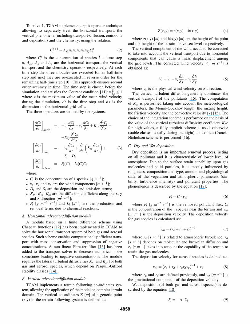
emission pre-processor POEM-CDII, addressed to the esti-mation of emission fields, (2) the CALMET meteorologicalmodel [7], which generates the meteorological input drivingTCAM and (3) a pre-processors which provides initial andboundary conditions required by TCAM (Figure 1). Thevalidation of the modelling system has been performed inthe frame of CityDelta-CAFE project (6th EU EnvironmentalAction Programme) [8] .

Fig. 1. Scheme of GAMES modelling system

II. MODEL DESCRIPTION

TCAM (Transport and Chemical Aerosol Model) is amultiphase three-dimensional Eulerian grid model, in terrain-following co-ordinate system. The model formalizes thephysical and chemical phenomena involved in the formationof secondary air pollution in heterogeneous phase. Thepollutant evolution is computed solving, for each cell of thecomputational domain, the following mass-balance equation:

∂Ci

∂ t= Ti + Ri + Di + Si (1)

where:

• Ci is the concentration of species i [g m−3];• Ti is the transport/diffusion term;• Ri the heterogeneous chemical term;• Di include the wet and the dry deposition;• Si is the emission term.

The chemical and physical phenomena occur simultane-ously in atmosphere but solving 1 for each domain cell wouldbe too time and memory expensive [9].

Proceedings of the44th IEEE Conference on Decision and Control, andthe European Control Conference 2005Seville, Spain, December 12-15, 2005

WeIA20.6

0-7803-9568-9/05/$20.00 ©2005 IEEE 4857

To solve 1, TCAM implements a split operator techniqueallowing to separately treat the horizontal transport, thevertical phenomena (including transport-diffusion, emissionsand deposition) and the chemistry, using the relation:

Cn+1i = AxyAzAcAcAzAxyC

ni (2)

where Cni is the concentration of species i at time step

n, Axy, Az and Ac are the horizontal transport, the verticaltransport and the chemistry operators respectively. At eachtime step the three modules are executed for an half-timestep and next they are re-executed in reverse order for theremaining half-time step [10]. This approach ensures secondorder accuracy in time. The time step is chosen before thesimulation and satisfies the Courant condition [11]: v δ t

δx ≤ 1where v is the maximum value of the mean wind velocityduring the simulation, δ t is the time step and δx is thedimension of the horizontal grid cells.

The three operators are defined by the systems:

[∂Ci

∂ t

]horiz

= −vx∂Ci

∂x− vy

∂Ci

∂y+ Kxx

∂ 2Ci

∂ 2x+

+Kyy∂ 2Ci

∂ 2y[∂Ci

∂ t

]vert

= −vz∂Ci

∂ z+

∂∂ z

(Kzz

∂Ci

∂ z

)+ (3)

+Si −Di[∂Ci

∂ t

]chem

= Pi(C)−Li(C)Ci

where:

• Ci is the concentration of i species [g m−3];• vx, vy and vz are the wind components [m s−1];• Di and Si are the deposition and emission terms;• Kxx, Kyy, Kzz are the diffusion coefficient along the x, y

and z direction [m2 s−1];• Pi [g m−3 s−1] and Li [s−1] are the production and

removal terms due to chemical reactions.

A. Horizontal advection/diffusion module

A module based on a finite difference scheme usingChapeau functions [12] has been implemented in TCAM tosolve the horizontal transport system of both gas and aerosolspecies. Such scheme enables computationally efficient trans-port with mass conservation and suppression of negativeconcentrations. A non linear Forester filter [13] has beenadded to the transport solver to decrease numerical noisesometimes leading to negative concentrations. The modulerequires the lateral turbulent diffusivities Kxx and Kyy for bothgas and aerosol species, which depend on Pasquill-Giffordstability classes [14].

B. Vertical advection/diffusion module

TCAM implements a terrain following co-ordinates sys-tem, allowing the application of the model on complex terraindomain. The vertical co-ordinates Z [m] of a generic point(x,y) in the terrain following system is defined as:

Z(x,y) = z(x,y)−h(x,y) (4)

where z(x,y) [m] and h(x,y) [m] are the height of the pointand the height of the terrain above sea level respectively.

The vertical component of the wind needs to be correctedto take into account the vertical transport due to horizontalcomponents that can cause a mass displacement amongthe grid levels. The corrected wind velocity Vz [m s−1] isobtained as:

Vz = vz − vxδhδx

− vyδhδy

(5)

where vz is the physical wind velocity on z direction.The vertical turbulent diffusion generally dominates the

vertical transport of the pollutants [15]. The computationof Kzz is performed taking into account the meteorologicalparameters: the Monin-Obukhov length, the mixing height,the friction velocity and the convective velocity [7] [15]. Thechoice of the integration scheme is performed on the basis ofthe value of the vertical turbulent diffusivity coefficient Kzz:for high values, a fully implicit scheme is used, otherwise(stable classes, usually during the night), an explicit Cranck-Nicholson scheme is performed [16].

C. Dry and Wet deposition

Dry deposition is an important removal process, actingon all pollutant and it is characteristic of lower level ofatmosphere. Due to the surface retain capability upon gasmolecules and solid particles, it is mostly influenced byroughness, composition and type, amount and physiologicalstate of the vegetation and atmospheric parameters (sta-bility, turbulence intensity) and pollutant properties. Thephenomenon is described by the equation [18]:

Fi = Ci · vdi (6)

where Fi [g m−2 s−1] is the removed pollutant flux, Ci

is the concentration of the i species near the terrain and vdi

[m s−1] is the deposition velocity. The deposition velocityfor gas species is calculated as:

vdi = (ra + rd + rc)−1 (7)

where ra [s m−1] is related to atmospheric turbulence, rd

[s m−1] depends on molecular and brownian diffusion andrc [s m−1] takes into account the capability of the terrain toretain the gas molecules.

The deposition velocity for aerosol species is defined as:

vdi = (ra + rd + rardvg)−1 + vg (8)

where ra and rd are defined previously, and vg [m s−1] isthe gravitational component of the deposition velocity.

Wet deposition (of both gas and aerosol species) is de-scribed by the equation [18]:

Fi = −Λ ·Ci (9)

4858

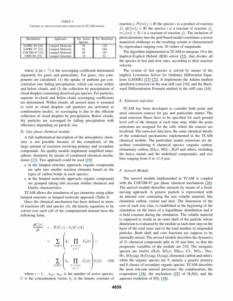
TABLE I

CHEMICAL MECHANISM IMPLEMENTED IN TCAM MODEL

Mechanism Approach No. Active No. ReactionsSpecies

SAPRC-90 [20] Lumped Molecule 54 128SAPRC-97 [21] Lumped Molecule 82 184COCOH-97 [24] Lumped Molecule 95 187

CBIV-90 [19] Lumped Structure 32 81

where Λ [m s−1] is the scavenging coefficient determinedseparately for gases and particulates. For gases, two com-ponents are calculated: (1) the uptake of ambient gas con-centration into falling precipitation, which can occur withinand below clouds, and (2) the collection by precipitation ofcloud droplets containing dissolved gas species. For particles,separate in-cloud and below-cloud scavenging coefficientsare determined. Within clouds, all aerosol mass is assumedto exist in cloud droplets (all particles are activated ascondensation nuclei), so scavenging is due to the efficientcollection of cloud droplets by precipitation. Below clouds,dry particles are scavenged by falling precipitation withefficiency depending on particle size.

D. Gas phase chemical module

A full mathematical description of the atmospheric chem-istry is not possible because of the complexity of thelarge amount of reactions involving primary and secondarycompounds. Air quality models implement simplified atmo-spheric chemistry by means of condensed chemical mecha-nisms [17]. Two approach could be used [19]:

• in the lumped structure approach, organic compoundsare split into smaller reaction elements based on thetypes of carbon bonds in each species;

• in the lumped molecule approach, organic compoundsare grouped taking into account similar chemical andkinetic characteristics.

TCAM allows the simulation of gas chemistry using eitherlumped structure or lumped molecule approach (Table I).

Once the chemical mechanism has been defined in termsof reactions (R) and species (S), the kinetic equations to besolved over each cell of the computational domain have thefollowing form:

dCi(t)dt

= Pi (C,t)−Li (C,t)Ci

= ∑j∈Q(i)

⎛⎜⎜⎝k j ∏

k ∈ rc( j)k �= j

Ck(t)

⎞⎟⎟⎠+

− ∑j∈R(i)

⎛⎜⎜⎝k j ∏

k ∈ rc( j)k �= j

Ck(t)

⎞⎟⎟⎠Ci(t) (10)

where i = 1, . . .nact , nact is the number of active species,C is the concentration vector, k j is the kinetic constant of

reaction j, P(i)={ j ∈ R/ the species i is a product of reactionj}, Q(i)={ j ∈ R/ the species i is a reactant of reaction j},rc( j)={i ∈ S/ i is a reactant of reaction j}. The inclusion ofphotochemistry into the grid-based model constitutes a severenumerical challenge as the resulting system is characterizedby eigenvalues ranging over 10 orders of magnitude.

The algorithm implemented in TCAM to integrate 10 is theImplicit-Explicit Hybrid (IEH) solver [22], that divides allthe species in fast and slow ones, according to their reactionvelocity.

The system of fast species is solved by means of theimplicit Livermore Solver for Ordinary Differential Equa-tions (LSODE) [23] [22]. It implements the Adams method(predictor-corrector) in the non-stiff case [16], and the Back-ward Differentiation Formula method in the stiff case [16].

E. Emission injection

TCAM has been developed to consider both point andareal emission sources for gas and particulate matter. Theareal emission fluxes have to be specified for each groundlevel cell of the domain at each time step, while the pointemissions are assigned for the cells where the sources arelocalized. The emission data have the same chemical detailsof the condensed mechanisms implemented in the TCAMchemical module. The particulate matter emissions are de-scribed considering 6 chemical species (organic carbon,elementary carbon, SO4=, NO3-, H2O and others, includingthe heavy metals and the undefined compounds), and sizebins ranging from 0 to 11.4 µm.

F. Aerosol Module

The aerosol module implemented in TCAM is coupledwith the COCOH-97 gas phase chemical mechanism [26].The aerosol module describes aerosols by means of a fixed-moving approach. A generic particle is represented withan internal core containing the non volatile material, likeelemental carbon, crustal and dust. The dimension of thecore of each size class is established at the beginning of thesimulation on the basis of a logarithmic distribution and itis held constant during the simulation. The volatile materialis supposed to reside in an outer shell of the particle whosedimension is evaluated by the module at each time step on thebasis of the total mass and of the total number of suspendedparticles. Both shell and core fractions are suppose to beinternally mixed. The aerosol module describes the dynamicsof 21 chemical compounds split in 10 size bins, so that theprognostic variables of the module are 210. The inorganicspecies are twelve (H2O, SO4=, NH4+, Cl-, NO3-, Na+,H+, SO2(aq), H2O2(aq), O3(aq), elemental carbon and other),while the organic species are 9, namely a generic primaryand 8 classes of secondary organic species. TCAM describesthe most relevant aerosol processes: the condensation, theevaporation [18], the nucleation [25] of H2SO4 and theaqueous oxidation of SO2 [18].

4859

III. MODEL VALIDATION

A. Model Setup

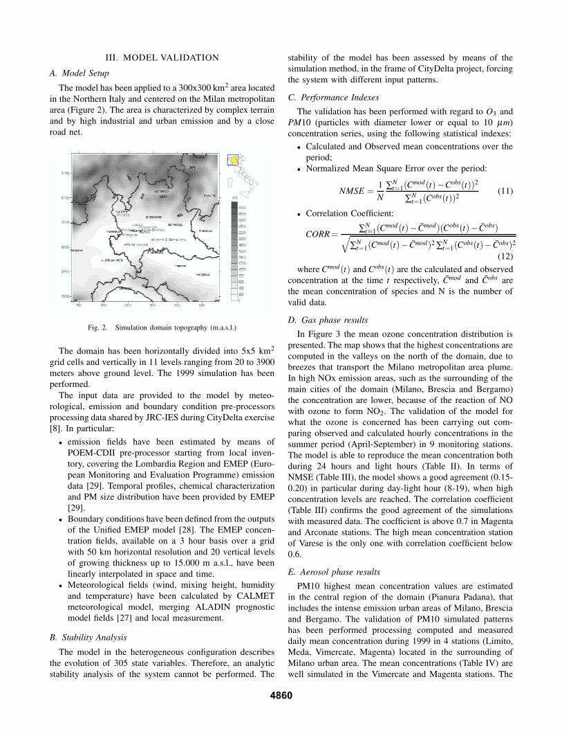
The model has been applied to a 300x300 km2 area locatedin the Northern Italy and centered on the Milan metropolitanarea (Figure 2). The area is characterized by complex terrainand by high industrial and urban emission and by a closeroad net.

Fig. 2. Simulation domain topography (m.a.s.l.)

The domain has been horizontally divided into 5x5 km2

grid cells and vertically in 11 levels ranging from 20 to 3900meters above ground level. The 1999 simulation has beenperformed.

The input data are provided to the model by meteo-rological, emission and boundary condition pre-processorsprocessing data shared by JRC-IES during CityDelta exercise[8]. In particular:

• emission fields have been estimated by means ofPOEM-CDII pre-processor starting from local inven-tory, covering the Lombardia Region and EMEP (Euro-pean Monitoring and Evaluation Programme) emissiondata [29]. Temporal profiles, chemical characterizationand PM size distribution have been provided by EMEP[29].

• Boundary conditions have been defined from the outputsof the Unified EMEP model [28]. The EMEP concen-tration fields, available on a 3 hour basis over a gridwith 50 km horizontal resolution and 20 vertical levelsof growing thickness up to 15.000 m a.s.l., have beenlinearly interpolated in space and time.

• Meteorological fields (wind, mixing height, humidityand temperature) have been calculated by CALMETmeteorological model, merging ALADIN prognosticmodel fields [27] and local measurement.

B. Stability Analysis

The model in the heterogeneous configuration describesthe evolution of 305 state variables. Therefore, an analyticstability analysis of the system cannot be performed. The

stability of the model has been assessed by means of thesimulation method, in the frame of CityDelta project, forcingthe system with different input patterns.

C. Performance Indexes

The validation has been performed with regard to O3 andPM10 (particles with diameter lower or equal to 10 µm)concentration series, using the following statistical indexes:

• Calculated and Observed mean concentrations over theperiod;

• Normalized Mean Square Error over the period:

NMSE =1N

∑Nt=1(C

mod(t)−Cobs(t))2

∑Nt=1(C

obs(t))2(11)

• Correlation Coefficient:

CORR =∑N

t=1(Cmod(t)− C̄mod)(Cobs(t)− C̄obs)√

∑Nt=1(C

mod(t)− C̄mod)2 ∑Nt=1(C

obs(t)− C̄obs)2

(12)

where Cmod(t) and Cobs(t) are the calculated and observedconcentration at the time t respectively, C̄mod and C̄obs arethe mean concentration of species and N is the number ofvalid data.

D. Gas phase results

In Figure 3 the mean ozone concentration distribution ispresented. The map shows that the highest concentrations arecomputed in the valleys on the north of the domain, due tobreezes that transport the Milano metropolitan area plume.In high NOx emission areas, such as the surrounding of themain cities of the domain (Milano, Brescia and Bergamo)the concentration are lower, because of the reaction of NOwith ozone to form NO2. The validation of the model forwhat the ozone is concerned has been carrying out com-paring observed and calculated hourly concentrations in thesummer period (April-September) in 9 monitoring stations.The model is able to reproduce the mean concentration bothduring 24 hours and light hours (Table II). In terms ofNMSE (Table III), the model shows a good agreement (0.15-0.20) in particular during day-light hour (8-19), when highconcentration levels are reached. The correlation coefficient(Table III) confirms the good agreement of the simulationswith measured data. The coefficient is above 0.7 in Magentaand Arconate stations. The high mean concentration stationof Varese is the only one with correlation coefficient below0.6.

E. Aerosol phase results

PM10 highest mean concentration values are estimatedin the central region of the domain (Pianura Padana), thatincludes the intense emission urban areas of Milano, Bresciaand Bergamo. The validation of PM10 simulated patternshas been performed processing computed and measureddaily mean concentration during 1999 in 4 stations (Limito,Meda, Vimercate, Magenta) located in the surrounding ofMilano urban area. The mean concentrations (Table IV) arewell simulated in the Vimercate and Magenta stations. The

4860

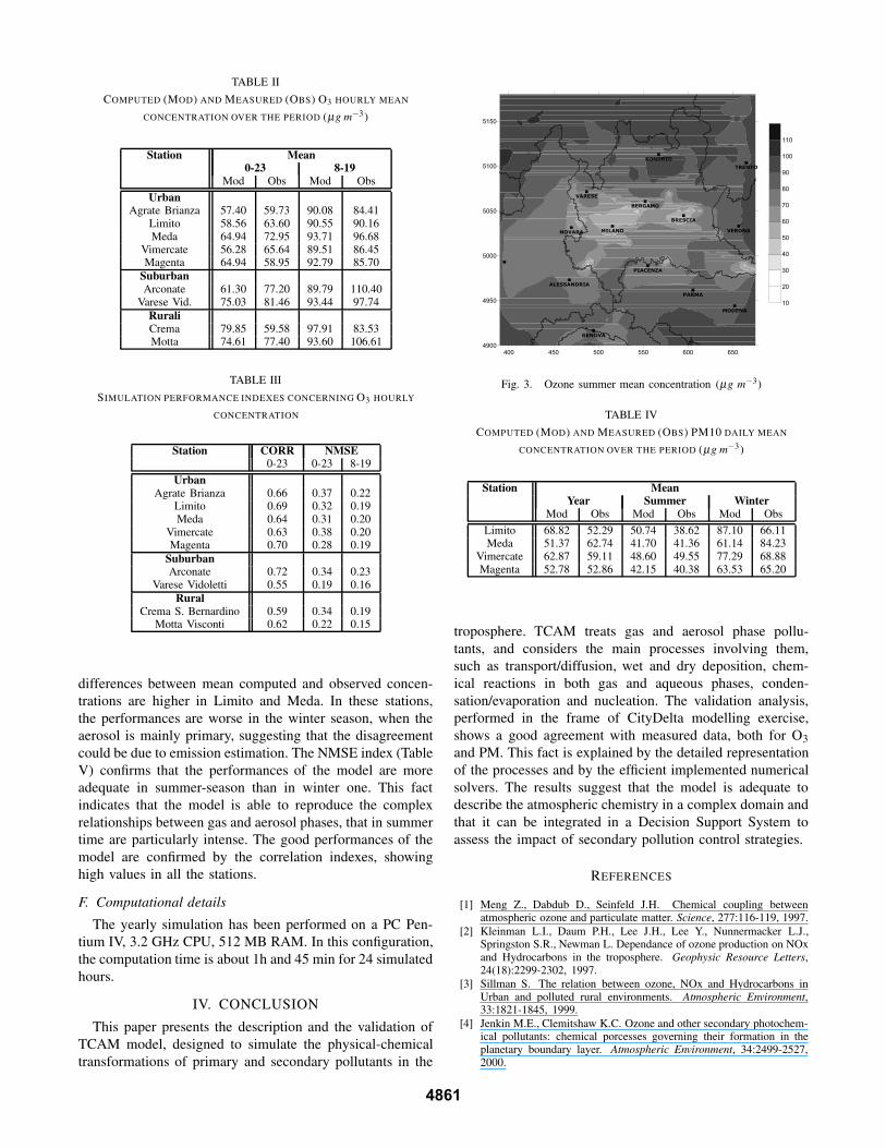
TABLE II

COMPUTED (MOD) AND MEASURED (OBS) O3 HOURLY MEAN

CONCENTRATION OVER THE PERIOD (µg m−3)

Station Mean0-23 8-19

Mod Obs Mod Obs

UrbanAgrate Brianza 57.40 59.73 90.08 84.41

Limito 58.56 63.60 90.55 90.16Meda 64.94 72.95 93.71 96.68

Vimercate 56.28 65.64 89.51 86.45Magenta 64.94 58.95 92.79 85.70

SuburbanArconate 61.30 77.20 89.79 110.40

Varese Vid. 75.03 81.46 93.44 97.74RuraliCrema 79.85 59.58 97.91 83.53Motta 74.61 77.40 93.60 106.61

TABLE III

SIMULATION PERFORMANCE INDEXES CONCERNING O3 HOURLY

CONCENTRATION

Station CORR NMSE0-23 0-23 8-19

UrbanAgrate Brianza 0.66 0.37 0.22

Limito 0.69 0.32 0.19Meda 0.64 0.31 0.20

Vimercate 0.63 0.38 0.20Magenta 0.70 0.28 0.19

SuburbanArconate 0.72 0.34 0.23

Varese Vidoletti 0.55 0.19 0.16Rural

Crema S. Bernardino 0.59 0.34 0.19Motta Visconti 0.62 0.22 0.15

differences between mean computed and observed concen-trations are higher in Limito and Meda. In these stations,the performances are worse in the winter season, when theaerosol is mainly primary, suggesting that the disagreementcould be due to emission estimation. The NMSE index (TableV) confirms that the performances of the model are moreadequate in summer-season than in winter one. This factindicates that the model is able to reproduce the complexrelationships between gas and aerosol phases, that in summertime are particularly intense. The good performances of themodel are confirmed by the correlation indexes, showinghigh values in all the stations.

F. Computational details

The yearly simulation has been performed on a PC Pen-tium IV, 3.2 GHz CPU, 512 MB RAM. In this configuration,the computation time is about 1h and 45 min for 24 simulatedhours.

IV. CONCLUSION

This paper presents the description and the validation ofTCAM model, designed to simulate the physical-chemicaltransformations of primary and secondary pollutants in the

Fig. 3. Ozone summer mean concentration (µg m−3)

TABLE IV

COMPUTED (MOD) AND MEASURED (OBS) PM10 DAILY MEAN

CONCENTRATION OVER THE PERIOD (µg m−3)

Station MeanYear Summer Winter

Mod Obs Mod Obs Mod Obs

Limito 68.82 52.29 50.74 38.62 87.10 66.11Meda 51.37 62.74 41.70 41.36 61.14 84.23

Vimercate 62.87 59.11 48.60 49.55 77.29 68.88Magenta 52.78 52.86 42.15 40.38 63.53 65.20

troposphere. TCAM treats gas and aerosol phase pollu-tants, and considers the main processes involving them,such as transport/diffusion, wet and dry deposition, chem-ical reactions in both gas and aqueous phases, conden-sation/evaporation and nucleation. The validation analysis,performed in the frame of CityDelta modelling exercise,shows a good agreement with measured data, both for O3

and PM. This fact is explained by the detailed representationof the processes and by the efficient implemented numericalsolvers. The results suggest that the model is adequate todescribe the atmospheric chemistry in a complex domain andthat it can be integrated in a Decision Support System toassess the impact of secondary pollution control strategies.

REFERENCES

[1] Meng Z., Dabdub D., Seinfeld J.H. Chemical coupling betweenatmospheric ozone and particulate matter. Science, 277:116-119, 1997.

[2] Kleinman L.I., Daum P.H., Lee J.H., Lee Y., Nunnermacker L.J.,Springston S.R., Newman L. Dependance of ozone production on NOxand Hydrocarbons in the troposphere. Geophysic Resource Letters,24(18):2299-2302, 1997.

[3] Sillman S. The relation between ozone, NOx and Hydrocarbons inUrban and polluted rural environments. Atmospheric Environment,33:1821-1845, 1999.

[4] Jenkin M.E., Clemitshaw K.C. Ozone and other secondary photochem-ical pollutants: chemical porcesses governing their formation in theplanetary boundary layer. Atmospheric Environment, 34:2499-2527,2000.

4861

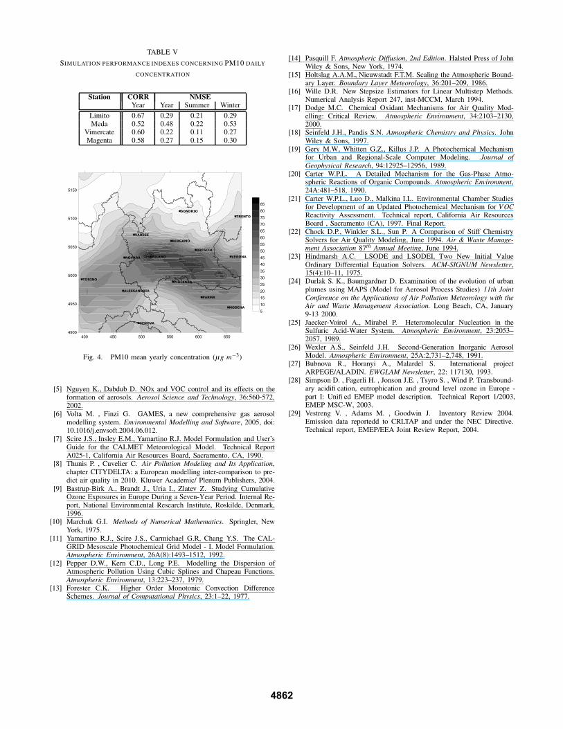
TABLE V

SIMULATION PERFORMANCE INDEXES CONCERNING PM10 DAILY

CONCENTRATION

Station CORR NMSEYear Year Summer Winter

Limito 0.67 0.29 0.21 0.29Meda 0.52 0.48 0.22 0.53

Vimercate 0.60 0.22 0.11 0.27Magenta 0.58 0.27 0.15 0.30

Fig. 4. PM10 mean yearly concentration (µg m−3)

[5] Nguyen K., Dabdub D. NOx and VOC control and its effects on theformation of aerosols. Aerosol Science and Technology, 36:560-572,2002.

[6] Volta M. , Finzi G. GAMES, a new comprehensive gas aerosolmodelling system. Environmental Modelling and Software, 2005, doi:10.1016/j.envsoft.2004.06.012.

[7] Scire J.S., Insley E.M., Yamartino R.J. Model Formulation and User’sGuide for the CALMET Meteorological Model. Technical ReportA025-1, California Air Resources Board, Sacramento, CA, 1990.

[8] Thunis P. , Cuvelier C. Air Pollution Modeling and Its Application,chapter CITYDELTA: a European modelling inter-comparison to pre-dict air quality in 2010. Kluwer Academic/ Plenum Publishers, 2004.

[9] Bastrup-Birk A., Brandt J., Uria I., Zlatev Z. Studying CumulativeOzone Exposures in Europe During a Seven-Year Period. Internal Re-port, National Environmental Research Institute, Roskilde, Denmark,1996.

[10] Marchuk G.I. Methods of Numerical Mathematics. Springler, NewYork, 1975.

[11] Yamartino R.J., Scire J.S., Carmichael G.R, Chang Y.S. The CAL-GRID Mesoscale Photochemical Grid Model - I. Model Formulation.Atmospheric Environment, 26A(8):1493–1512, 1992.

[12] Pepper D.W., Kern C.D., Long P.E. Modelling the Dispersion ofAtmospheric Pollution Using Cubic Splines and Chapeau Functions.Atmospheric Environment, 13:223–237, 1979.

[13] Forester C.K. Higher Order Monotonic Convection DifferenceSchemes. Journal of Computational Physics, 23:1–22, 1977.

[14] Pasquill F. Atmospheric Diffusion, 2nd Edition. Halsted Press of JohnWiley & Sons, New York, 1974.

[15] Holtslag A.A.M., Nieuwstadt F.T.M. Scaling the Atmospheric Bound-ary Layer. Boundary Layer Meteorology, 36:201–209, 1986.

[16] Wille D.R. New Stepsize Estimators for Linear Multistep Methods.Numerical Analysis Report 247, inst-MCCM, March 1994.

[17] Dodge M.C. Chemical Oxidant Mechanisms for Air Quality Mod-elling: Critical Review. Atmospheric Environment, 34:2103–2130,2000.

[18] Seinfeld J.H., Pandis S.N. Atmospheric Chemistry and Physics. JohnWiley & Sons, 1997.

[19] Gery M.W, Whitten G.Z., Killus J.P. A Photochemical Mechanismfor Urban and Regional-Scale Computer Modeling. Journal ofGeophysical Research, 94:12925–12956, 1989.

[20] Carter W.P.L. A Detailed Mechanism for the Gas-Phase Atmo-spheric Reactions of Organic Compounds. Atmospheric Environment,24A:481–518, 1990.

[21] Carter W.P.L., Luo D., Malkina I.L. Environmental Chamber Studiesfor Development of an Updated Photochemical Mechanism for VOCReactivity Assessment. Technical report, California Air ResourcesBoard , Sacramento (CA), 1997. Final Report.

[22] Chock D.P., Winkler S.L., Sun P. A Comparison of Stiff ChemistrySolvers for Air Quality Modeling, June 1994. Air & Waste Manage-ment Association 87th Annual Meeting, June 1994.

[23] Hindmarsh A.C. LSODE and LSODEI, Two New Initial ValueOrdinary Differential Equation Solvers. ACM-SIGNUM Newsletter,15(4):10–11, 1975.

[24] Durlak S. K., Baumgardner D. Examination of the evolution of urbanplumes using MAPS (Model for Aerosol Process Studies) 11th JointConference on the Applications of Air Pollution Meteorology with theAir and Waste Management Association. Long Beach, CA, January9-13 2000.

[25] Jaecker-Voirol A., Mirabel P. Heteromolecular Nucleation in theSulfuric Acid-Water System. Atmospheric Environment, 23:2053–2057, 1989.

[26] Wexler A.S., Seinfeld J.H. Second-Generation Inorganic AerosolModel. Atmospheric Environment, 25A:2,731–2,748, 1991.

[27] Bubnova R., Horanyi A., Malardel S. International projectARPEGE/ALADIN. EWGLAM Newsletter, 22: 117130, 1993.

[28] Simpson D. , Fagerli H. , Jonson J.E. , Tsyro S. , Wind P. Transbound-ary acidifi cation, eutrophication and ground level ozone in Europe -part I: Unifi ed EMEP model description. Technical Report 1/2003,EMEP MSC-W, 2003.

[29] Vestreng V. , Adams M. , Goodwin J. Inventory Review 2004.Emission data reportedd to CRLTAP and under the NEC Directive.Technical report, EMEP/EEA Joint Review Report, 2004.

4862