A Series Journal of the Chinese Physical SocietyDistributed by IOP Publishing

Online: http://www.iop.org/journals/cplhttp://cpl.iphy.ac.cn

CHINESE PHYSICAL SOCIETY

ISSN: 0256-307X

中国物理快报

ChinesePhysicsLetters

CHIN. PHYS. LETT. Vol. 26,No. 7 (2009) 078903

Information Feedback Strategies in a Signal Controlled Network with OverlappedRoutes *

TIAN Li-Jun(田丽君)1, HUANG Hai-Jun(黄海军)1**, LIU Tian-Liang(刘天亮)21School of Economics and Management, Beijing University of Aeronautics and Astronautics, Beijing 100083

2School of Economics and Management, Tsinghua university, Beijing 100084

(Received 2 October 2008)We investigate the effects of four different information feedback strategies on the dynamics of traffic, travel-ers’ route choice and the resultant system performance in a signal controlled network with overlapped routes.Simulation results given by the cellular automaton model show that the system purpose-based mean velocityfeedback strategy and the congestion coefficient feedback strategy have more advantages in improving networkutilization efficiency and reducing travelers’ travel times. The travel time feedback strategy and the individualpurposed-based mean velocity feedback strategy behave slightly better to ensure user equity.

PACS: 89. 40.−a, 64. 60. Aq, 02. 60. Cb

Advanced traveler information systems (ATIS) aregenerally believed to be efficient in some aspects suchas improving individuals’ route choices, alleviatingroad congestion and enhancing road usage by provid-ing real-time information of traffic condition to roadusers.[1−4] The dynamics of traffic flow with real-timetraffic information has attracted much attention fromresearchers and has become one of the most impor-tant research directions in the traffic field.[5,6] Wahleet al.[7] firstly investigated the effect of the undesir-able feedback loop on the stability of traffic patternsusing a travel time feedback strategy (TTFS) in a sim-ple network with two routes. In terms of the lag ef-fect of the TTFS,[8,9] Wahle et al.[10] further discussedthe possibility of the global density feedback strat-egy (GDFS) and the mean velocity feedback strat-egy (MVFS), and showed that the nature of the infor-mation overly influences the potential benefits of theATIS. Recently, Wang et al.[11] improved the GDFSand brought forward a more effective congestion coef-ficient feedback strategy (CCFS).

The above-mentioned works were carried out insimple networks where there is only one origin-destination (OD) pair connected by two identicallength routes. In reality, there generally exist multipleOD pairs, heterogeneous routes between each OD pairand overlapped parts among multiple routes. It is thusinteresting to explore the effects of different informa-tion feedback strategies on dynamics of traffic, travel-ers’ route choice and the resultant system performancein complex networks. On the base of the study of Tianet al.,[12] in this Letter we further compare the simula-tion results in a signal controlled network under fourinformation feedback strategies, namely travel timefeedback strategy, mean velocity feedback strategyfrom individual purpose (MVFS IP), mean velocityfeedback strategy from system purpose (MVFS SP)and congestion coefficient feedback strategy.

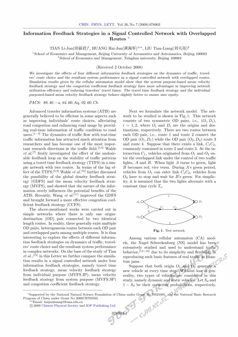
Next we formulate the network model. The net-work to be studied is shown in Fig. 1. This networkconsists of two symmetric OD pairs, i.e., (𝑂𝑖, 𝐷𝑖),𝑖 = 1, 2, where 𝑂𝑖 and 𝐷𝑖 are the origins and des-tinations, respectively. There are two routes betweeneach OD pair, i.e., route 1 and route 2 connect theOD pair (𝑂1, 𝐷1) while the OD pair (𝑂2, 𝐷2) route 3and route 4. Suppose that there exists a link, 𝐶1𝐶2,commonly contained in route 2 and route 3. At the in-tersection 𝐶1, vehicles originated from 𝑂1 and 𝑂2 en-ter the overlapped link under the control of two trafficlights, 𝐴 and 𝐵. When light 𝐴 turns to green, light𝐵 becomes red, vice versa. During 𝐴’s green period,vehicles from 𝑂1 can enter link 𝐶1𝐶2, vehicles from𝑂2 have to stop and wait for 𝐵’s green. For simplic-ity, it is assumed that the two lights alternate with aconstant time cycle 𝑇𝑠.

1

4

3

2

O1

C1 C2

O2

D1

D2

Fig. 1. Test network.

Among various cellular automaton (CA) mod-els, the Nagel–Schreckenberg (NS) model has beenextensively studied and used to understand trafficbehavior,[13−16] due to its simplicity and flexibility inreproducing such basic features of real traffic as phan-tom jams.

Suppose that both origin 𝑂1 and 𝑂2 generate anew vehicle at every time step. Without loss of gen-erality, two types of vehicles are considered in thisstudy, namely dynamic and static vehicles. Let 𝑆𝑑 and1 − 𝑆𝑑 be their occurring probabilities, respectively.

*Supported by the National Natural Science Foundation of China under Grant No 70521001, and the National Basic ResearchProgram of China under Grant No 2006CB705503.

**Email: haijunhuang@buaa.edu.cnc○ 2009 Chinese Physical Society and IOP Publishing Ltd

078903-1

CHIN. PHYS. LETT. Vol. 26,No. 7 (2009) 078903

The static vehicles do not carry the information dis-played on the ATIS board, and enter a route randomly.On the other hand, the dynamic ones receive the infor-mation and make decisions of route choice accordingto the feedback information provided by ATIS.[7] If anew vehicle enters the network, its movement followsthe dynamics of the NS model and is finally removedfrom the network once it reaches the destination. Ifa vehicle cannot enter the network, it is deleted fromthe system for simplicity.

11

11

L

L

L1

L1

L2

L3

L3

Fig. 2. Cell automata model.

Each link in the network is subdivided into dis-crete cells, as displayed in Fig. 2. The physical lengthof each cell is 7.5 m. Let 𝐿, ��, 𝐿1, 𝐿2, and 𝐿3 be thenumber of cells on route 1 or route 4, the number ofcells on route 2 or route 3, the number of cells on link𝑂1𝐶1 or 𝑂2𝐶1, the number of cells on the overlappedpart 𝐶1𝐶2, and the number of cells on link 𝐶2𝐷1 or𝐶2𝐷2, respectively. In this way, �� = 𝐿1 + 𝐿2 + 𝐿3

holds.

The state of vehicle 𝑛 is determined by its speed 𝑣𝑛

and the position 𝑥𝑛. The value of 𝑣𝑛 lies between 0and 𝑣max. Here the maximum speed 𝑣max is givenand fixed. Furthermore, let 𝑔𝑛 = 𝑥𝑛+1 − 𝑥𝑛 − 1and 𝑠𝑛 be the distance between vehicle 𝑛 and vehi-cle 𝑛 + 1 and the distance between vehicle 𝑛 and in-tersection 𝐶1, respectively. The NS mechanism con-sidering a signalized intersection can be decomposedto the following four rules (parallel dynamics): rule1: acceleration, 𝑣𝑛 ← min(𝑣𝑛 + 1, 𝑣max); rule 2: de-celeration, 𝑣safe

𝑛 ← min(𝑣𝑛, 𝑔𝑛, 𝑠𝑛), if vehicle 𝑛 hasnot arrived at intersection 𝐶1 and the red light ison, and 𝑣safe

𝑛 ← min(𝑣𝑛, 𝑔𝑛), otherwise; rule 3: ran-dom brake, with a certain brake probability 𝑝, do𝑣random

𝑛 ← max(𝑣safe𝑛 − 1, 0); and rule 4: movement,

𝑥𝑛 ← 𝑥𝑛 + 𝑣random𝑛 . Here 𝑣safe

𝑛 and 𝑣random𝑛 represent

the safe speed and the random brake speed of vehicle𝑛, respectively. Without loss of generality, it is sup-posed that the maximum speed 𝑣max = 3 and randombrake probability 𝑝 = 0.25 in our simulation.

We now describe the four real-time informationfeedback strategies to be investigated in detail.

TTFS: Every dynamic vehicle chooses a route withthe shortest time. At the beginning of the simulation,

there is not a vehicle arriving at destination, so thatevery dynamic vehicle makes the route choice onlyaccording to the static information displayed on theboard at origin. When a vehicle arrives at destinationand leaves the network, the travel time experiencedby this vehicle is immediately displayed on the infor-mation board.

MVFS IP: All dynamic vehicles are assumed tochoose routes with the shortest times determined in-stantaneously. Unlike TTFS, however, the instanta-neous travel times displayed on the information boardsare obtained on the base of mean velocities of vehicleson routes. At every time step, each vehicle reportsits current speed to a traffic control center. The cen-ter calculates the mean velocity of all vehicles on aroute according to the received speeds. Taking theOD pair (𝑂1, 𝐷1) as an example, we let the instanta-neous travel time of route 1 be the ratio of its lengthover the mean velocity of all vehicles on it. The in-stantaneous travel time of route 2 can be computedas follows: 𝑇 = 𝐿1/𝑉1 + 𝐿2/𝑉2 + 𝐿3/𝑉3, where 𝑉1,𝑉2 and 𝑉3 are the mean velocities of all vehicles onlink 𝑂1𝐶1, 𝐶1𝐶2 and 𝐶2𝐷1, respectively. The dy-namic vehicle from 𝑂1 chooses a route on the base ofmin{𝐿/𝑉, 𝑇 , 𝑇} where 𝑉 is the mean velocity of allvehicles on route 1.

MVFS SP: All dynamic vehicles are assumed tochoose routes with larger mean velocities. At everytime step, each vehicle on routes reports its currentspeed to the traffic control center. The mean velocityof all vehicles on a route is computed and displayedon the information boards. In our study, the mean ve-locity of route 2 is 𝑉 = ��/(𝐿1𝑉1 + 𝐿2/𝑉2𝑉2 + 𝐿3/𝑉3),where 𝑉1, 𝑉2 and 𝑉3 are the mean velocities of all vehi-cles on link 𝑂1𝐶1, 𝐶1𝐶2 and 𝐶2𝐷1, respectively. Thedynamic vehicle from 𝑂1 chooses a route on the baseof max{𝑉, 𝑉 }. Clearly, MVFS SP is different fromMVFS IP when 𝐿 = ��.

0.8 1.2 1.6 2.0 0.8 1.2 1.6 2.0300

400

500

600

700

800

t ↼104↽ t ↼104↽

t ↼1

04↽

t ↼1

04↽

Tra

vel tim

e Route 1 Route 2

0.1

0.2

0.3

0.4

0.5

Flu

x

Route 1

Route 2

(a) (b)

200 400 600 8001.7

1.8

1.9

2.0

x0 200 400 600 800

1.7

1.8

1.9

2.0

x

250 300 350 4001.94

1.95

1.96T104

(c) (d)

Fig. 3. Simulation results under TTFS: the travel times(a), the average fluxes (b), the vehicles’ spatial-temporaldiagrams on route 1 (c), on route 2 (d). The inset in (d)is the amplified one of a local part.

CCFS: All dynamic vehicles are assumed to choose

078903-2

CHIN. PHYS. LETT. Vol. 26,No. 7 (2009) 078903

a route with smaller congestion coefficient. At everytime step, each vehicle on routes, being either staticor dynamic one, sends such information as its posi-tion and speed to a navigation system. The trafficcontrol center computes the congestion coefficient foreach route according to the received information. Thecongestion coefficient (CC)[11] of a route can be mea-sured as follows: 𝐶𝐶 =

∑𝑚𝑖=1 𝑛𝑤

𝑖 , where 𝑛𝑖 is the num-ber of vehicles included into the 𝑖th congestion cluster.A traffic cluster means that vehicles are close to eachother without a gap between any two of them. It isclear that by increasing the cluster size, the travel timeof the last vehicle of a cluster would become longer.Therefore, an exponent 𝑤 is used to represent the non-linear correlation between cluster size and congestioncoefficient. When 𝑤 = 1, the CCFS is similar to theglobal density feedback strategy (GDFS) investigatedby Wahle et al.[10] For simplicity, we let 𝑤 = 2 in thisstudy. One can find more details about the CCFS inWang et al.[11]

(a) (b)

0.8 1.2 1.6 2.00.1

0.2

0.3

0.4

0.5

Flu

x

Route 1 Route 2

1.7

1.8

1.9

2.0

t (1

04)

1.7

1.8

1.9

2.0(c) (d)

0 200 400 600 800x

200 400 600 800x

0.8 1.2 1.6 2.0300

400

500

600

700

800

t (104) t (104)

t (1

04)

Tra

vel tim

e Route 1Route 2

250 300 350 4001.91

1.92

1.93 T104

Fig. 4. Simulation results under MVFS IP. Explanationsfor (a)–(d) are given in the caption of Fig. 3.

The network utilization efficiency can be charac-terized by a measure called flux. It is the product ofmean velocity and global density in a manner.

Now, taking link 𝑂1𝐶1, route 2 and OD pair(𝑂1, 𝐷1) as examples, we define link average flux,route average flux and OD pair average flux.[12] Theaverage flux of link 𝑂1𝐶1 is defined by 𝐹1 = 𝑉1𝜌 =𝑉1𝑁/𝐿1, where 𝜌, 𝑁 and 𝐿1 represent the global den-sity, the number of vehicles on link 𝑂1𝐶1 and thelength of link 𝑂1𝐶1, respectively.

The average flux of route 2 is actually equal to theaverage flux of link 𝐶2𝐷1, 𝐹route2 = 𝐹3, where 𝐹3 rep-resents the average flux of link 𝐶2𝐷1. The averageflux of OD pair (𝑂1, 𝐷1) is the sum of the averagefluxes of two routes which connect it, 𝐹 (𝑂1, 𝐷1) =𝐹route1 + 𝐹route2, where 𝐹route1 and 𝐹route2 representthe average fluxes of route 1 and route 2, respectively.

Finally, we report the simulation results obtainedfrom the last 20000 iterations, excluding the initial5000 time steps. Considering the symmetric structureof the test network, without loss of generality, we only

analyze the statistic outputs associated with OD pair(𝑂1, 𝐷1). In the simulation, we let 𝐿 = 1000, �� = 800,𝐿2 = 20, 𝑇𝑠 = 10, 𝑆𝑑 = 0.7 and the overlapped partbe always located in the middle of route 2 (or route3).

Figures 3–6 show the simulation results abouttravel times, average fluxes and vehicles’ spatial-temporal diagrams on route 1 and route 2 un-der the four information feedback strategies, TTFS,MVFS IP, MVFS SP and CCFS, respectively. Fromthese figures, we have the following findings.

(i) In contrast with the other three strategies, theTTFS leads to great oscillations in travel time and av-erage flux, a trend of enlarging the periods of vehicles’spatial-temporal evolution, and much queuing beforethe intersection 𝐶1 (the black triangles in Fig. 3(d)).This further validates that the TTFS indeed has a lageffect in guiding traffic, as reported in Refs. [7–12].

(a) (b)

300

400

500

600

700

800

Tra

vel tim

eRoute 1 Route 2

0.8 1.2 1.6 2.00.1

0.2

0.3

0.4

0.5

t ↼104↽

t ↼1

04↽

0.8 1.2 1.6 2.0

t ↼104↽

Flu

x Route 1 Route 2

1.7

1.8

1.9

2.0

t ↼1

04↽

1.7

1.8

1.9

2.0

0 200 400 600 800x

(c)

200 400 600 800x

250 300 350 4001.96

1.97

1.98T104

(d)

Fig. 5. Simulation results under MVFS SP. Explanationsfor (a)–(d) are given in the caption of Fig. 3.

(a) (b)

300

400

500

600

700

800

Tra

vel tim

e

Route 1

Route 2

0.8 1.2 1.6 2.00.1

0.2

0.3

0.4

0.5

Flu

x Route 1

Route 2

0 200 400 600 800x

200 400 600 800x

1.7

1.8

1.9

2.0(c)

250 300 350 4001.91

1.92

1.93

t ↼104↽

t ↼1

04↽

1.7

1.8

1.9

2.0

t ↼1

04↽

0.8 1.2 1.6 2.0

t ↼104↽

T104

(d)

Fig. 6. Simulation results under CCFS. Explanations for(a)–(d) are given in the caption of Fig. 3.

(ii) Regardless of the adopted information feed-back strategy, the average flux on route 1 is largerthan that on route 2 although route 2 is shorter. Thisis mainly because route 2 is overlapped by route 3 andinstalled with a signal light. Clearly, the strategies

078903-3

CHIN. PHYS. LETT. Vol. 26,No. 7 (2009) 078903

MVFS SP and CCFS are more sensitive to the routeoverlap and traffic signal than the other two strategies.This makes more vehicles be guided to select route 1.

(iii) The CCFS produces relatively small oscilla-tions in travel time and average flux. Implementinga crude equilibrium of travel times on two routes re-quires less time steps than other strategies. The num-ber of congestion clusters before the signal light is themost, but the size of each cluster is the smallest.

(iv) Although the strategies TTFS and MVFS IPare designed from individual purpose, they have noobvious advantages in improving individuals’ routechoice and reducing the travel times.

In the following, we investigate how the length ofroute 2, ��, affects the average flux of OD pair (𝑂1, 𝐷1)and the travel time difference between route 1 androute 2 under the four strategies.

Fig. 7. Four strategies give (a) the average flux of ODpair (𝑂1, 𝐷1) and (b) the travel time difference betweenroute 1 and route 2, against route 2’s length.

Fig. 8. Four strategies generate the average flux of ODpair (𝑂1, 𝐷1) against 𝑆𝑑, where (a) 𝑇𝑠 = 5, (b) 𝑇𝑠 = 10,(c) 𝑇𝑠 = 15 and (d) 𝑇𝑠 = 20.

Figure 7(a) shows that in comparison with theother two strategies from system purposes, the av-erage fluxes of OD pair (𝑂1, 𝐷1) under TTFS andMVFS IP change greatly with increasing ��, particu-larly when the length of route 2 is less than 600 cells.When �� > 600, the average fluxes under MVFS SP

and CCFS become unchanged basically. On average,the MVFS SP and CCFS can implement more fluxesthan other two strategies.

The user equity can be characterized by the traveltime difference between route 1 and route 2. Figure7(b) shows that, with increasing ��, the user equity byMVFS SP and CCFS almost decrease linearly. How-ever, this linear property does not hold under TTFSand MVFS IP. For each value of ��, except the valueswithin [600, 900], the absolute value of ∆𝑡 by TTFSor MVFS IP is not larger than that by MVFS SP orCCFS.

Now, we turn to investigate the effects of vehi-cle types (denoted by the occurring probability of dy-namic vehicles) on flux, under different informationservice strategies and different traffic light cycles. InFig. 8, it can be seen that, though different informa-tion feedback strategies and different traffic light cy-cles are adopted, the average flux of OD pair (𝑂1, 𝐷1)always first increases slowly and then decreases rapidlywith an increase of dynamic travelers. When 𝑆𝑑 ≤ 0.5,there is no obvious difference among the performancescaused by the four feedback strategies. This might bebecause few dynamic vehicles accept the informationservice so that static vehicles dominate the evolutionof the system. When 𝑆𝑑 is larger than 0.5, the effectdifference becomes gradually more obvious. It is foundthat CCFS is the best strategy and MVFS SP is thesecond best before 𝑆𝑑 increases to a certain criticalvalue, labeled by 𝑆𝑑 𝐶 in Fig. 8.

References

[1] Mahmassani H S and Liu Y H 1999 Transp. Res. C 7 91[2] Ben-Akiva M, De Palama A and Kaysi I 1991 Transp. Res.

A 25 251[3] Adler J L and Blue V J 1998 Transp. Res. C 6 157[4] Huang H J, Liu T L and Yang H 2008 J. Adv. Transport.

42 111[5] Chowdhury D, Santen L and Schadschneider A 2000 Phys.

Rep. 329 199[6] Helbing D 2001 Rev. Mod. Phys. 73 1067[7] Wahle J, Bazzan A L C, Klugl F and Schreckenberg M 2000

Physica A 287 669[8] Lee K, Hui P M, Wang B H and Johnson N F 2001 Soc. J.

Phys. Jpn. 70 3507[9] Fu C J, Wang B H, Yin C Y and Gao K 2006 Acta Phys.

Sin. 55 4032 (in Chinese)[10] Wahle J, Bazzan A L C, Klugl F and Schreckenberg M 2002

Transport. Res. C 10 399[11] Wang W X, Wang B H, Zheng W C, Yin C Y and Zhou T

2005 Phys. Rev. E 72 066702[12] Tian L J, Liu T L and Huang H J 2008 Acta Phys. Sin.

57 2122 (in Chinese)[13] Nagel K and Schreckenberg M 1992 J. Phys. I 2 2221[14] Li K P and Gao Z Y 2004 Chin. Phys. Lett. 21 2120[15] Chen T, Jia B, Li X G, Jiang R and Gao Z Y 2008 Chin.

Phys. Lett. 25 2795[16] Wang B H, Hui P M and Gu G Q 1997 Chin. Phys. Lett.

14 202

078903-4