Travelling wave solutions in the generalized Hirota-Satsuma coupled KdV system

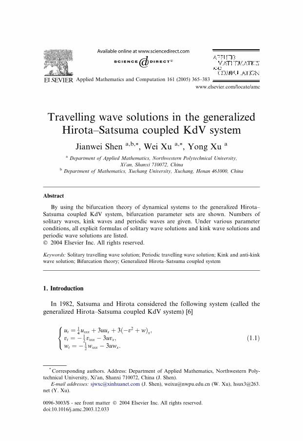
Applied Mathematics and Computation 161 (2005) 365–383

www.elsevier.com/locate/amc

Travelling wave solutions in the generalizedHirota–Satsuma coupled KdV system

Jianwei Shen a,b,*, Wei Xu a,*, Yong Xu a

a Department of Applied Mathematics, Northwestern Polytechnical University,

Xi’an, Shanxi 710072, Chinab Department of Mathematics, Xuchang University, Xuchang, Henan 461000, China

Abstract

By using the bifurcation theory of dynamical systems to the generalized Hirota–

Satsuma coupled KdV system, bifurcation parameter sets are shown. Numbers of

solitary waves, kink waves and periodic waves are given. Under various parameter

conditions, all explicit formulas of solitary wave solutions and kink wave solutions and

periodic wave solutions are listed.

� 2004 Elsevier Inc. All rights reserved.

Keywords: Solitary travelling wave solution; Periodic travelling wave solution; Kink and anti-kink

wave solution; Bifurcation theory; Generalized Hirota–Satsuma coupled system

1. Introduction

In 1982, Satsuma and Hirota considered the following system (called the

generalized Hirota–Satsuma coupled KdV system) [6]

* Co

technic

E-m

net (Y

0096-3

doi:10.

ut ¼ 14uxxx þ 3uux þ 3ð�v2 þ wÞx;

vt ¼ � 12vxxx � 3uvx;

wt ¼ � 12wxxx � 3uwx:

8<: ð1:1Þ

rresponding authors. Address: Department of Applied Mathematics, Northwestern Poly-

al University, Xi’an, Shanxi 710072, China (J. Shen).

ail addresses: [email protected] (J. Shen), [email protected] (W. Xu), hsux3@263.

. Xu).

003/$ - see front matter � 2004 Elsevier Inc. All rights reserved.

1016/j.amc.2003.12.033

mail to: [email protected]

366 J. Shen et al. / Appl. Math. Comput. 161 (2005) 365–383

When w ¼ 0, (1.1) reduces to be the well known Hirota–Satsuma coupled Kdvequation [9]. This equation starts from the 4-reduction of the KP hierarchy.For the background materials of model equations, we refer to the paper [6,9]

and the references therein. Recently, Tam et al. [3] obtained some exact solu-

tion of (1.1) in terms of the Hirota’s bilinear method, and Yan [11] used ex-

tended Jacobian elliptic function expansion method to construct new doubly

periodic solution of (1.1), including solitary wave solutions and trigonometric

function solutions. Unfortunately, the results in [3,11] are not complete since

the authors did not study the bifurcation behaviors of phase portraits for the

corresponding travelling wave equations. In this paper, we will considerbifurcation problem of solitary waves, kink waves and periodic waves for (1.1),

by using the bifurcation theory of dynamical system [2,7,8,10]. Under fixed

parameter conditions, all explicit formulas of solitary wave , kink wave and

periodic wave solutions can be easily obtained.

To find the travelling wave solutions of (1.1), we first consider the travelling

wave solutions in the form

uðx; tÞ ¼ uðnÞ; vðx; tÞ ¼ vðnÞ; wðx; tÞ ¼ wðnÞ; n ¼ kðx� ktÞ; ð1:2Þ

where k denotes the wave speed. Therefore (1.1) reduces to be

�ku0 ¼ 14k2u000 þ 3uu0 þ 3ð�v2 þ wÞ0; ð1:3aÞ

kv0 ¼ 12k2v000 þ 3uv0; ð1:3bÞ

kw0 ¼ 12k2w000 � 3uw0; ð1:3cÞ

where ‘‘0’’ is the derivative with respect to n.Now we consider the dynamical behaviors of (1.3) on the plane

u ¼ av2 þ bvþ c; w ¼ A1vþ B1; ð1:4Þ

where a, b, c, A1,B1 are constants to be determined later.Substituting (1.4) into (1.3b) and (1.3c) and integrating once we know that

(1.3b) and (1.3c) give rise to the same equation

k2v00 ¼ �2av3 � 3bv2 þ 2ðk � 3cÞvþ c1: ð1:5Þ

Obviously, (1.5) has the following first integral:

k2ðv0Þ2 ¼ �av4 � 2bv3 þ 2ðk � 3cÞv2 þ 2c1vþ c2; ð1:6Þ

where c1, c2 are integration constant. From (1.4)–(1.6) we obtain

k2u00 ¼ �6a2v4 � 12abv3 þ ð8ak � 24ac � 3b2Þv2

þ ð6c1a þ 2kb � 6cbÞvþ ðc1b þ 2ac2Þ: ð1:7Þ

J. Shen et al. / Appl. Math. Comput. 161 (2005) 365–383 367

Integrating (1.3a) once we have

1

4k2u00 þ 3

2u2 þ kuþ 3ð�v2 þ wÞ þ c3 ¼ 0; ð1:8Þ

where c3 is an integration constant. Inserting (1.4) and (1.7) into (1.8) yields

3ak � 3ac þ 34

b2 � 3 ¼ 0; ð1:9aÞ

ac1 þ bc þ bk þ 2A1 ¼ 0; ð1:9bÞ

1

4ð2ac2 þ bc1Þ þ

3

2c2 þ kc þ 3B1 þ c3 ¼ 0: ð1:9cÞ

We find from (1.9) that

a ¼ b2 � 44ðc � kÞ ; A1 ¼ �ðb2 � 4Þc1

8ðc � kÞ � 12bðk þ cÞ;

B1 ¼ �ðb2 � 4Þc224ðc � kÞ � 1

12bc1 �

1

2c2 � 1

3kc � 1

3c3: ð1:10Þ

In this paper, we always assume that Eq. (1.1) satisfies (1.10). Under the

condition (1.10), it is easy to see that system (1.5) has the same topological

phase portraits as (1.1). Therefore, we only consider the system (1.5). Eq. (1.5)can become the following two-dimensional system:

dvdn

¼ y;dydn

¼ � 1

k2ð2av3 þ 3bv2 þ 2ð3c � kÞv� c1Þ: ð1:11Þ

Obviously, (1.11) is a Hamiltonian system with Hamiltonian function

Hðv; yÞ ¼ 12y2 þ 1

k21

2av4

�þ bv3 þ ð3c � kÞv2 � c1v

�: ð1:12Þ

All travelling wave solutions of (1.1) under the condition (1.10) can be

determined by the phase orbits of (1.11). Suppose that vðx; tÞ ¼ vðx� ctÞ ¼ vðnÞis a continuous solution of Eq. (1.1) for n 2 ð�1;1Þ, and limn!1 vðnÞ ¼ a1,limn!�1 vðnÞ ¼ b1. It is well known that (i) vðx; tÞ is called a solitary wavesolution if a1 ¼ b1. (ii) vðx; tÞ is called a kink (or anti-kink) solution is a1 6¼ b1.Usually, a solitary wave solution of (1.1) corresponds to a homoclinic orbit of

(1.11); A kink (or anti-kink) wave solution of (1.1) corresponds to a hetero-

clinic orbit of (1.11); and a periodic travelling wave solution of (1.1) corre-

sponds to a periodic orbit of (1.11) (see [4,5]). Thus, to investigate all

bifurcations of solitary waves, kink waves and periodic waves of Eq. (1.1), weshould find all bounded solutions of (1.11) depending on the parameter space

of this system. The bifurcation theory of dynamical systems (see [2,8,10]) plays

an important role in our study.


The paper is organized as follows. In Section 2, we consider the dynamical

behaviors of (1.1) in the plane (1.4) and give the bifurcation set and phaseportraits. In Section 3, we show all explicit formulae of solitary wave and kink

(anti-kink) wave under given parameter conditions. In Section 4, all explicit

formulae of periodic wave solutions are given. Our study results give rise to

complete description of all travelling waves of (1.1) under the condition (1.10)

and contain some results in [3,11] as special examples.

2. Bifurcations of phase portraits of (1.1)

In this section, we will study bifurcation set and phase portraits of (1.1)

when parameters k, a, b, c, k and c1 are varied from (1.11). On the ðv; yÞ-phaseplane, the abscissas of equilibrium points of system (1.11) are the zeros of

f ðvÞ ¼ v3 þ 3b2a v

2 þ 3c�ka v� c1

2a. Let ðve; yÞ be an equilibrium of (1.11). At this

point, the determinant of the linearized system of (1.11) has the form

Jðve; 0Þ ¼ 2ak2 f

0ðveÞ. By using the bifurcation theory of planar dynamical system,we know that if Jðve; 0Þ > 0 (or < 0), then the equilibrium ðve; 0Þ is a center (orsaddle point); if Jðve; 0Þ ¼ 0 and the Poincar�e index of ðve; 0Þ is zero, then theequilibrium ðve; 0Þ is a cusp.

Case I. 3c � k ¼ 0Making the transformation

ffiffiffiffi2ak2

qn ¼ s, y !

ffiffiffiffi2ak2

qy for a > 0 or

ffiffiffiffiffiffi�2ak2

qn ¼ s,

y !ffiffiffiffiffiffi�2ak2

qy for a < 0, (1.11) becomes the following two-dimensional system:

dvds

¼ y;dyds

¼ �ðv3 þ av2 � cÞ; ð2:1Þ

where

a ¼ 3b2a

; c ¼ c12a

and when a > 0 (or < 0), then the sign in the right hand side of secondequation of ((2.1) is ‘‘)’’ (or ‘‘+’’). System (2.1) is a Hamiltonian system with

Hamiltonian function

Hðv; yÞ ¼ 12y2 � 1

4v4

�þ 13av3 � cv

�: ð2:2Þ

By using the above discussion at the beginning of Section 2 to do qualitative

analysis, we obtain the following results: on the ða; cÞ-parameter plane, thereare three bifurcation curves (see Fig. 1)

L1 : c ¼ 0; L2 : c ¼2

27a3; L3 : c ¼

4

27a3: ð2:3Þ

–10

–5

0

5

10

c

–4 –2 2 4

a

Fig. 1. The partition of the ða; cÞ-parameter strip of (2.1) for 3c � k ¼ 0.


From the above discussions we have the partition in ða; cÞ-parameter planeby curves Li, i ¼ 1, 2, 3 shown in Fig. 1 where

ðAÞ 0 < c < L1; ðBÞ L2 < c < L3; ðCÞ c > L3 > 0;

ðDÞ L2 < c < L1; ðEÞ L3 < c < L2; ðF Þ c < L3 < 0:

Corresponding to regions ðAÞ–ðF Þ of the bifurcation set of ða; cÞ, phaseportraits of (2.1) can be shown in Figs. 2 and 3, respectively.

Case II. 3c � k > 0.Making the transformation

ffiffiffiffiffiffiffiffiffiffiffi2ð3c�kÞ

k2

qn ¼ f,

ffiffiffiffiffiffiffijaj3c�k

qv ! v,

ffiffiffiffiffiffiffiffiffiffiffiffiffik2jaj

2ð3c�kÞ3

qy ! y, (1.11)

becomes the following two-dimensional system:

dvdf

¼ y;dydf

¼ �ð�v3 þ ev2 þ v� gÞ; ð2:4Þ

where

e ¼ 3b

2jaj12ð3c � kÞ

12

; g ¼ jaj12c1

2ð3c � kÞ32

and when a > 0 (or < 0), the sign of the term v3 in the right hand side of thesecond equation of (2.4) is ‘‘+’’ (or ‘‘)’’), system (2.4) is a Hamiltonian systemwith Hamiltonian function

Hðv; yÞ ¼ 12y2 � 1

4v4 þ e

3v3 þ 1

2v2 � gv: ð2:5Þ

(1) Suppose that a > 0. Write that f1ðvÞ ¼ v3 þ ev2 þ v� g,f 0ðvÞ ¼ 3v2 þ 2evþ 1. Thus f 0ðvÞ has two zeros at v1;2 ¼ �e�

ffiffiffiffiffiffiffie2�3

p

3. Obvi-

ously, v1;2 is real if and only if jejPffiffiffi3

p. Hence, in this situation there exists

three bifurcation curves (see Fig. 4)

-4

-2

2

4

y

-4 -3 -2 -1 1

x

-3

-2

-1

1

2

3

y

-3 -2 -1 1

x

-2

-1

0

1

2

y

-3 -2 -1 1

x

-3

-2

-1

0

1

2

3

y

-3 -2 -1 1

x

(1) (2) (3) (4)

-4

-2

2

4

y

-3 -2 -1 1 2

x

-1

-0.5

0

0.5

1

y

0.2 0.4 0.6 0.8 1 1.2 1.4 1.6

x

-4

-2

2

4

y

-1 1 2 3 4

x

-3

-2

-1

0

1

2

3

y

-1 1 2 3

x

(5) (6) (7) (8)

-2

-1

0

1

2

y

-1 1 2 3

x

-3

-2

-1

1

2

3

y

-1 1 2 3

x

-4

-2

0

2

4

y

-2 -1 1 2 3

x

-2

-1

0

1

2

y

-1.6 -1.4 -1.2 -1 -0.8 -0.6 -0.4 -0.2

x

(9) (10) (11) (12)

Fig. 2. Phase portraits of (2.1) for a > 0 and 3c � k ¼ 0. (1) ða; cÞ 2 L1, (2) ða; cÞ 2 ðAÞ, (3)ða; cÞ 2 L2, (4) ða; cÞ 2 ðBÞ, (5) ða; cÞ 2 L3, (6) ða; cÞ 2 ðCÞ, (7) ða; cÞ 2 L1, (8) ða; cÞ 2 ðDÞ, (9)ða; cÞ 2 L2, (10) ða; cÞ 2 E, (11) ða; cÞ 2 L3, (12) ða; cÞ 2 ðF Þ.


L4 : g ¼ �227

ðe2 � 3Þ32 þ 2

27e3 � 1

3e; L5 : g ¼ 2

27e3 � 1

3e;

L6 : g ¼ 2

27ðe2 � 3Þ

32 þ 2

27e3 � 1

3e: ð2:6Þ

From the above discussions we have the partition in ðe; gÞ-parameter planeby curves Li, i ¼ 4, 5, 6 shown in Fig. 4 where

ðI1Þ g < L4; ðII1Þ L4 < g < L5; ðIII1Þ L5 < g < L6;

ðIV1Þ g > L6:

-10

-5

5

10

y

-4 -2 2

x

-4

-2

0

2

4

y

-4 -3 -2 -1 1 2

x

-4

-2

0

2

4

y

-4 -3 -2 -1 1 2

x

-4

-2

0

2

4

y

-4 -3 -2 -1 1 2

x

(1) (2) (3) (4)

-4

-2

0

2

4

y

-4 -3 -2 -1 1 2

x

-10

-5

5

10

y

-3 -2 -1 1 2 3

x

-10

-5

5

10

y

-2 2 4

x

-4

-2

0

2

4

y

-2 -1 1 2 3 4

x

(5) (6) (7) (8)

-4

-2

0

2

4

y

-2 -1 1 2 3 4

x

-4

-2

0

2

4

y

-2 -1 1 2 3 4

x

-4

-2

0

2

4

y

-2 -1 1 2 3 4

x

-4

-2

0

2

4

y

-2 -1 1 2

x

(9) (10) (11) (12)

Fig. 3. Phase portraits of (2.1) for a < 0 and 3c � k ¼ 0. (1) ða; cÞ 2 L1, (2) ða; cÞ 2 ðAÞ, (3)ða; cÞ 2 L2, (4) ða; cÞ 2 ðBÞ, (5) ða; cÞ 2 L3, (6) ða; cÞ 2 ðCÞ, (7) ða; cÞ 2 L1, (8) ða; cÞ 2 ðDÞ, (9)ða; cÞ 2 L2, (10) ða; cÞ 2 E, (11) ða; cÞ 2 L3, (12) ða; cÞ 2 ðF Þ.


Corresponding to regions ðI1Þ–ðIV1Þ of the bifurcation set of ðe; gÞ, the bifur-cations of phase portraits of (2.4) can be shown in Fig. 5.

(2) Suppose that a < 0. On the ðe; gÞ-parameter plane, there are three bifurca-tion curves (see Fig. 6)

L7 : g ¼ � 2

27ðe2 þ 3Þ

32 þ 2

27e3 þ 1

3e; L8 : g ¼ 2

27e3 þ 1

3e;

L9 : g ¼ 2

27ðe2 þ 3Þ

32 þ 2

27e3 þ 1

3e: ð2:7Þ

From the above discussion we have the partition in ðe; gÞ-parameter planeby curves Li, i ¼ 7, 8, 9, shown in Fig. 6 where

–10

–5

5

10

g

–4 –2 2 4

e

Fig. 4. The partition of the ðe; gÞ-parameter strip of (2.4) for a > 0 and 3c � k > 0.

–2

–1

0

1

2

y

–3 –2.5 –2 –1.5 –1 –0.5

x

–0.4

–0.2

0

0.2

0.4

y

–1.5 –1 –0.5

x

–0.3

–0.2

–0.1

0

0.1

0.2

0.3

y

–1.6 –1.4 –1.2 –1 –0.8 –0.6 –0.4 –0.2

x

(1) (2) (3)

–0.2

–0.1

0

0.1

0.2

y

–1.4 –1.2 –1 –0.8 –0.6 –0.4 –0.2 0.2

x

–0.3

–0.2

–0.1

0

0.1

0.2

0.3

y

–1.4 –1.2 –1 –0.8 –0.6 –0.4 –0.2 0.2

x

–0.4

–0.2

0

0.2

0.4

y

–1.2 –1 –0.8 –0.6 –0.4 –0.2 0.2

x

–0.4

–0.2

0.2

0.4

y

–0.4 –0.2 0 .2 0.4

x

(4) (5) (6) (7)

Fig. 5. Phase portraits of (2.4) for a > 0 and 3c � k > 0 (1) ðe; gÞ 2 I1, (2) ðe; gÞ 2 ðL4Þ,(3) ðe; gÞ 2 ðII1Þ, (4) ðe; gÞ 2 ðL5Þ, (5) ðe; gÞ 2 ðIII1Þ, (6) ðe; gÞ 2 L6, (7) ðe; gÞ 2 ðIV1Þ.


ðI2Þ g < L7; ðII2Þ L7 < g < L8; ðIII2Þ L8 < g < L9; ðIV2Þ g > L9:

Corresponding to regions ðI2Þ–ðIV2Þ of the bifurcation set of ðe; gÞ, phaseportraits of (2.4) can be shown in Fig. 7.

Case III. 3c � k < 0.

–10

–5

5

10

g

–4 –2 2 4

e

Fig. 6. The partition of the ðe; gÞ-parameter strip of (2.4) for a < 0 and 3c � k > 0.

–4

–2

0

2

4

y

–2 –1 1 2 3

x

–4

–2

0

2

4

y

–4 –3 –2 –1 1 2 3

x

–2

–1

0

1

2

y

–1 1 2

x

–4

–2

0

2

4

y

–2 –1 1 2 3

x

–4

–2

0

2

4

y

–2 –1 1 2 3

x

–4

–2

0

2

4

y

–2 –1 1 2 3

x

–4

–2

0

2

4

y

–2 –1 1 2 3

x

(1) (2) (3)

(4) (5) (6) (7)

Fig. 7. Phase portraits of (2.4) for a < 0 and 3c � k > 0. (1) ðe; gÞ 2 I2, (2) ðe; gÞ 2 ðL7Þ,(3) ðe; gÞ 2 ðII2Þ, (4) ðe; gÞ 2 ðL8Þ, (5) ðe; gÞ 2 ðIII2Þ, (6) ðe; gÞ 2 L9, (7) ðe; gÞ 2 ðIV2Þ.


Making the transformation

ffiffiffiffiffiffiffiffiffiffiffi2ðk�3cÞ

k2

qn ¼ 1,

ffiffiffiffiffiffiffijaj

k�3c

qv ! v,

ffiffiffiffiffiffiffiffiffiffiffiffiffik2jaj

2ðk�3cÞ3

qy ! y, (1.11)

becomes the following two-dimensional system:

dvd1

¼ y;dyd1

¼ �ð�v3 þ e1v2 � v� g1Þ; ð2:8Þ


where

–2 –1.5

Fig. 8

(3) ðe1

e1 ¼3b

2jaj12ðk � 3cÞ

12

; g1 ¼jaj

12c1

2ðk � 3cÞ32

and when a > 0 (or < 0), the sign of the term v3 in the right hand side of thesecond equation of (2.4) is ‘‘+’’ (or ‘‘)’’), system (2.4) is Hamiltonian system

with Hamiltonian function

Hðv; yÞ ¼ 12y2 � 1

4v4 þ e1

3v3 � 1

2v2 � g1v: ð2:9Þ

(1) Suppose that a > 0. On the ðe1; g1Þ-parameter plane, there are three bifur-cation curves, same as (2.7) shown in Fig. 6. From the above discussions we

have the following phase portraits (see Fig. 8).

(2) Suppose that a < 0. On the ðe1; g1Þ-parameter plane, there are three bifur-cation curves, same as (2.7) shown in Fig. 4. From the above discussions we

have the following phase portraits (see Fig. 9).

3. Solitary wave and kink wave solutions determined by (1.1)

In this section we will give all explicit solitary wave solutions and kink (or

anti-kink) wave solutions of (1.1) under given parameter conditions. By using

–1

–0.5

0

0.5

1

y

–2.8 –2.6 –2.4 –2.2 –2 –1.8

x

–4

–2

0

2

4

y

–2 –1 1 2 3

x

–1.5

–1

–0.5

0

0.5

1

1.5

y

–2 –1.5 –1 –0.5 0.5 1

x

–1

–0.5

0

0.5

1

y

–1 –0.5 0.5 1 1.5

x

–1.5

–1

–0.5

0

0.5

1

1.5

y

–2 –1.5 –1 –0.5 0.5 1 1.5

x

–1.5

–1

–0.5

0

0.5

1

1.5

y

–1.5 –1 –0.5 0.5 1 1.5

x

–1

–0.5

0

0.5

1

y

0.2 0.4 0.6 0.8 1 1.2 1.4 1.6

x

(1) (2) (3)

(4) (5) (6) (7)

. Phase portraits of (2.8) for a > 0 and 3c � k > 0. (1) ðe1; g1Þ 2 I2, (2) ðe1; g1Þ 2 ðL7Þ,; g1Þ 2 ðII2Þ, (4) ðe1; g1Þ 2 ðL8Þ, (5) ðe1; g1Þ 2 ðIII2Þ, (6) ðe1; g1Þ 2 L9, (7) ðe1; g1Þ 2 ðIV2Þ.

–4

–2

0

2

4

y

–1 1 2 3 4

x

–2

–1

0

1

2

y

–1 1 2

x

–2

–1

1

2

y

–1 –0.5 0.5 1 1.5 2 2.5

x

–2

–1

0

1

2

y

–1 –0.5 0.5 1 1.5 2 2.5

x

–1

–0.5

0

0.5

1

y

–0.5 0.5 1 1.5 2

x

–3

–2

–1

0

1

2

3

y

–1 1 2

x

–2

–1

0

1

2

y

–1 –0.5 0.5 1 1.5 2

x

(1) (2) (3)

(4) (5) (6) (7)

Fig. 9. Phase portraits of (2.8) for a < 0 and 3c � k < 0. (1) ðe1; g1Þ 2 I1, (2) ðe1; g1Þ 2 ðL4Þ, (3)ðe1; g1Þ 2 ðII1Þ, (4) ðe1; g1Þ 2 ðL5Þ, (5) ðe1; g1Þ 2 ðIII1Þ, (6) ðe1; g1Þ 2 L6, (7) ðe1; g1Þ 2 ðIV1Þ.


the the travelling wave system (1.11) and the Hamiltonian function (1.12) to do

the calculations with the aid of Maple. We have the following results:

Case I. 3c � k ¼ 0.Denote that v1 < v2 < v3 are the roots of v3 þ av2 � c ¼ 0,

X1i ¼ �2via� 3v2i , w1i ¼ 9v2i þ 6via� 2a2, a1i ¼ við3vi þ 2aÞ, C1i ¼ 24ð3vi þ aÞ,i ¼ 1; 2; 3, n ¼ kðx� ktÞ, s ¼

ffiffiffiffiffiffiffiffiffi�2a

pðx� ctÞ.

Suppose that a > 0.

(1) Corresponding to Figs. 2(1) and (7), (1.1) has the following solitary wave

solution with valley form and peak form, respectively:

vðsÞ ¼ �12a9þ 2a2s2 ;

uðsÞ ¼ av2ðsÞ þ bvðsÞ þ c; wðsÞ ¼ A1vðsÞ þ B1: ð3:1Þ

(2) Corresponding to Fig. 2(2), (4), (8) and (10), (1.1) has the following solitarywave solutions with valley form and peak form:

vðsÞ ¼ v2 þ72a12

72w12 expðffiffiffiffiffiffiffiX12

psÞ � expð�

ffiffiffiffiffiffiffiX12

psÞ � C12

;


(3) Corresponding to Fig. 2(3) and (9), (1.1) has the following solitary wave

solutions with valley and peak form:


vðsÞ ¼ � a3�

ffiffiffi6

p

3a sech

2ffiffiffi3

p

3s

!;



solution with peak form:

vðsÞ ¼ � 23aþ 12a

9� 2a2s2 ;


Suppose that a < 0.(5) Corresponding to Fig. 3(2) and (10), (1.1) has the following solitary wave

solution with valley form:

vðsÞ ¼ v3 �72a13

�72w13 expðffiffiffiffiffiffiffiffiffiffiffi�X13

psÞ þ expð�

ffiffiffiffiffiffiffiffiffiffiffi�X13

psÞ þ C13

;


(6) Corresponding to Fig. 3(3) and (9), (1.1) has the following kink and anti-

kink wave solutions:

vðsÞ ¼ � 13a�

ffiffiffi3

p

3a tanh

ffiffiffi6

p

6as

!;



solution with peak form:

vðsÞ ¼ v1 �72a11

72w11 expðffiffiffiffiffiffiffiffiffiffiffi�X11

psÞ � expð�


psÞ þ C11

;


Case II. 3c � k > 0.Denote v1 < v2 < v3 are the roots of �v3 þ ev2 þ v� g ¼ 0, f ¼ffiffiffiffiffiffiffiffiffiffiffiffiffiffiffiffiffiffiffi2ð3c � kÞ

pðx� ctÞ, and making the following v change to

ffiffiffiffiffiffiffijaj3c�k

qv, we can

obtain the solutions of (1.1).

Suppose a > 0

(1) Corresponding to Fig. 5(2), (1.1) has the following solitary wave solution

with valley form:


vðfÞ ¼ � 13eþ 1

3

ffiffiffiffiffiffiffiffiffiffiffiffiffie2 � 3

p� 12


p

9þ 2ðe2 � 3Þf2;

uðfÞ ¼ av2ðfÞ þ bvðfÞ þ c; wðfÞ ¼ A1vðfÞ þ B1: ð3:8Þ

(2) Corresponding to Fig. 5(3), (1.1) has the following solitary wave solutions

with valley and peak form:

vðfÞ ¼ v2 þ72X21

72a21 expðffiffiffiffiffiffiffiffiffiffiffi�X21

pfÞ � expð�


pfÞ � 24ðeþ 3v2Þ

;

uðfÞ ¼ av2ðfÞ þ bvðfÞ þ c; ðfÞ ¼ A1vðfÞ þ B1; ð3:9Þ

where

a21 ¼ 9þ 6v2 þ 9v22 � 2e2; X21 ¼ 3v22 þ 2v2eþ 1:

(3) Corresponding to Fig. 5(4), (1.1) has the following solitary wave solutionswith valley and peak form:

vðfÞ ¼ � 13e�

ffiffiffiffiffiffiffiffiffiffiffiffiffiffiffiffiffiffiffi6ðe2 � 3Þ

p3

sech

ffiffiffiffiffiffiffiffiffiffiffiffiffiffiffiffiffiffiffi3ðe2 � 3Þ

p3

f

!;

uðfÞ ¼ av2ðfÞ þ bvðfÞ þ c; ðfÞ ¼ A1vðfÞ þ B1: ð3:10Þ


with peak form:

vðfÞ ¼ � 13


p� 13eþ 64ð3� e2Þ

48ffiffiffiffiffiffiffiffiffiffiffiffiffie2 � 3

pþ exp �2

ffiffiffiffiffiffiffiffiffiffiffi2ðe2�3Þ

p3

f

� � ;

uðfÞ ¼ av2ðfÞ þ bvðfÞ þ c; ðfÞ ¼ A1vðfÞ þ B1: ð3:11Þ

Suppose that a < 0.(5) Corresponding to Fig. 7(3), (1.1) has the following solitary wave solution

with peak form:


72a22 expðffiffiffiffiffiffiffiX22

pfÞ þ expð�


pfÞ þ 24ðeþ 3v1Þ

;

uðfÞ ¼ av2ðfÞ þ bvðfÞ þ c; wðfÞ ¼ A1vðfÞ þ B1; ð3:12Þ

where

a22 ¼ 9þ 6v1e� 9v21 þ 2e2; X22 ¼ 3v21 � 2v1e� 1:

(6) Corresponding to Fig. 7(4), (1.1) has the following kink and anti-kink wave

solutions:


vðfÞ ¼ 13e�

ffiffiffi3

p

3

ffiffiffiffiffiffiffiffiffiffiffiffiffie2 þ 3

ptanh

ffiffiffi6

p

6


pf

!;

uðfÞ ¼ av2ðfÞ þ bvðfÞ þ c; wðfÞ ¼ A1vðfÞ þ B1: ð3:13Þ


with peak form:



pfÞ þ expð�


pfÞ þ 24ðe� 3v3Þ

;


where

a23 ¼ 9þ 6v1e� 9v23 þ 2e2; X23 ¼ 3v23 � 2v3e� 1:

Case III. 3c � k < 0.Denote v1 < v2 < v3 are the roots of �v3 þ e1v2 � v� g1 ¼ 0,

1 ¼ffiffiffiffiffiffiffiffiffiffiffiffiffiffiffiffiffiffiffi2ðk � 3cÞ

pðx� ctÞ, and making the following v change to

ffiffiffiffiffiffiffijaj

k�3c

qv, we can

obtain the solutions of (1.1).

Suppose that a > 0.


with valley form:

vð1Þ ¼ 13


q� 13e1 þ

6ffiffiffiffiffiffiffiffiffiffiffiffiffie21 þ 3

p�9þ 2ðe21 þ 3Þ12

;

uð1Þ ¼ av2ð1Þ þ bvð1Þ þ c; wð1Þ ¼ A1vð1Þ þ B1: ð3:15Þ

(2) Corresponding to Fig. 8(3) and (5), (1.1) has the following solitary wavesolutions with valley and peak form:

vð1Þ ¼ v2 �72X31


p1Þ � expð�


p1Þ þ 24ðe1 þ 3v2Þ

;

uð1Þ ¼ av2ð1Þ þ bvð1Þ þ c; wð1Þ ¼ A1vð1Þ þ B1; ð3:16Þwhere

a31 ¼ 9v22 þ 6v2e1 � 2e21 � 9; X31 ¼ 3v22 þ 2v2e1 � 1:

(3) Corresponding to Fig. 8(4), (1.1) has the following solitary wave solutionswith valley and peak form:

vð1Þ ¼ � 13e1 �

ffiffiffi6

p

3


qsech


pffiffiffi3

p 1

!;




with peak form:

vð1Þ ¼ � 13


q� 13e1 þ

12ffiffiffiffiffiffiffiffiffiffiffiffiffie21 þ 3

p9þ 2ðe21 þ 3Þ12

;


Suppose that a < 0.(5) Corresponding to Fig. 9(3), (1.1) has the following solitary wave solution

with peak form:

vð1Þ ¼ v1 þ72X32


p1Þ þ expð�


p1Þ þ 24ðe1 � 3v1Þ

;

uð1Þ ¼ av2ð1Þ þ bvð1Þ þ c; ð1Þ ¼ A1vð1Þ þ B1; ð3:19Þ

where

a32 ¼ �9v21 þ 6v1e1 þ 2e21 � 9; X32 ¼ 3v21 � 2v1e1 þ 1:

(6) Corresponding to Fig. 9(4), (1.1) has the following kink and anti-kink wave

solutions:

vð1Þ ¼ 13e1 �

ffiffiffi3

p

3


qtanh

ffiffiffi6

p

6


q1

!;



with valley form:

vð1Þ ¼ v3 þ72X33


p1Þ þ expð�


p1Þ þ 24ðe1 � 3v3Þ

;

uð1Þ ¼ av2ð1Þ þ bvð1Þ þ c; ð1Þ ¼ A1vð1Þ þ B1; ð3:21Þ

where

a33 ¼ �9v23 þ 6v3e1 þ 2e21 � 9; X33 ¼ 3v23 � 2v3e1 þ 1:

To sum up, from the above discussions, we have

Theorem 1. There are 21 parametric conditions of (1.1) such that (1.1) has 21formulae of solitary wave solutions, kinks and anti-kink wave solutions given by(3.1)–(3.21).


4. Periodic wave solutions determined by (1.1)

In this section, all the periodic wave solutions of (1.1) will be given. Denote

that snðu; kÞ, cnðu; kÞ, tnðu; kÞ are the Jacobian elliptic functions with themodulus k, KðkÞ is the complete elliptic integral of the first kind and EðkÞ is thecomplete elliptic integral of the second kind (see [1]).

Case I. 3c � k ¼ 0Suppose that a > 0.Denote m11 < m12 < m13 < m14 are the roots of 2h� 1

2v4 � 2

3av3 þ 2cv ¼ 0, h

is Hamiltonian value, s ¼ffiffiffiffiffi2a

pðx� ctÞ.

(1) Corresponding to Fig. 2(6) and (12), Eq. (1.1) has one family of smooth

periodic wave solutions.

(2) Corresponding to Fig. 2(1), (5), (7) and (11), Eq. (1.1) has two families of

smooth periodic wave solutions.

(3) Corresponding to Fig. 2(2)–(4) and (8)–(10), Eq. (1.1) has three families of

smooth periodic wave solutions.

These periodic wave solutions have the following parametric representation:

vðsÞ ¼m14ðm13 � m11Þ � m11ðm14 � m13Þsn2 sffiffi

2p

g11; k11

� �ðm13 � m11Þ þ ðm14 � m13Þsn2 sffiffi

2p

g11; k11

� � ;

uðsÞ ¼ av2ðsÞ þ bvðsÞ þ c; wðsÞ ¼ A1vðsÞ þ B1; ð4:1Þ

where

g11 ¼2ffiffiffiffiffiffiffiffiffiffiffiffiffiffiffiffiffiffiffiffiffiffiffiffiffiffiffiffiffiffiffiffiffiffiffiffiffiffiffiffiffiffiffiffiffiffiffi

ðm14 � m12Þðm13 � m11Þp ; k211 ¼

ðm14 � m13Þðm12 � m11Þðm14 � m12Þðm13 � m11Þ

:

Suppose that a > 0.Denote m21 < m22 < m23 < m24 are the roots of 2hþ 1

2v4 þ 2

3av3 � 2cv ¼ 0, h

is Hamiltonian value, s ¼ffiffiffiffiffiffiffiffiffi�2a

pðx� ctÞ.

Corresponding to Fig. 3(2)–(4) and (8)–(10), Eq. (1.1) has one family of

smooth periodic wave solution which have the following parametric repre-sentation:


2p

g21; k21

� �ðm23 � m21Þ � ðm24 � m21Þsn2 sffiffi

2p

g21; k21

� � ;

uðsÞ ¼ av2ðsÞ þ bvðsÞ þ c; wðsÞ ¼ A1vðsÞ þ B1; ð4:2Þ


where


ðm24 � m22Þðm23 � m21Þp ; k221 ¼


:

Case II. 3c � k > 0.

Suppose that a > 0.Denote m31 < m32 < m33 < m34 are the roots of 2h� 1

2v4 � 2

3ev3 � v2þ

2gv ¼ 0, h is Hamiltonian value, f ¼ffiffiffiffiffiffiffiffiffiffiffiffiffiffiffiffiffiffiffi2ð3c � kÞ

pðx� ctÞ, and making the fol-

lowing v change toffiffiffiffiffiffiffijaj3c�k

qv, we can obtain the solutions of (1.1).

(1) Corresponding to Fig. 5(1) and (7), Eq. (1.1) has one family of smoothperiodic wave solutions.

(2) Corresponding to Fig. 5(2) and (6), Eq. (1.1) has two families of smooth


(3) Corresponding to Fig. 5(3)–(5), Eq. (1.1) has three families of smooth peri-

odic wave solutions.


vðfÞ ¼m34ðm33 � m31Þ � m31ðm34 � m33Þsn2 fffiffi

2p

g31; k31

� �ðm33 � m31Þ þ ðm34 � m33Þsn2 sffiffi

2p

g31; k31

� � ;


where


ðm34 � m32Þðm33 � m31Þp ; k231 ¼


:

Suppose that a < 0.Denote m41 < m42 < m43 < m44 are the roots of 2hþ 1

2v4 þ 2

3ev3þ

v2 � 2gv ¼ 0, h is Hamiltonian value, f ¼ffiffiffiffiffiffiffiffiffiffiffiffiffiffiffiffiffiffiffi2ð3c � kÞ

pðx� ctÞ, and making the

following v change toffiffiffiffiffiffiffijaj3c�k


Corresponding to Fig. 7(3)–(5), Eq. (1.1) has one family of smooth periodic

wave solutions which have the following parametric representation:

vðfÞ ¼m44ðm43 � m41Þ � m43ðm44 � m41Þsn2 fffiffi

2p

g41; k41

� �ðm43 � m41Þ � ðm44 � m41Þsn2 fffiffi

2p

g41; k41

� � ;



where


ðm44 � m42Þðm43 � m41Þp ; k241 ¼


:

Case III. 3c � k < 0.Suppose that a > 0.Denote m51 < m52 < m53 < m54 are the roots of 2h� 1

2v4 � 2

3e1v3þ

v2 þ 2g1v ¼ 0, h is Hamiltonian value, 1 ¼ffiffiffiffiffiffiffiffiffiffiffiffiffiffiffiffiffiffiffi2ðk � 3cÞ


following v change toffiffiffiffiffiffiffijaj

k�3c


(1) Corresponding to Fig. 8(1) and (7), Eq. (1.1) has one family of smooth


(2) Corresponding to Fig. 8(2) and (6), Eq. (1.1) has two families of smoothperiodic wave solutions.

(3) Corresponding to Fig. 8(3)–(5), Eq. (1.1) has three families of smooth peri-

odic wave solutions.


vð1Þ ¼m54ðm53 � m51Þ � m51ðm54 � m53Þsn2 sffiffi

2p

g51; k51

� �ðm53 � m51Þ þ ðm54 � m53Þsn2 1ffiffi

2p

g51; k51

� � ;

uð1Þ ¼ av2ð1Þ þ bvð1Þ þ c; wð1Þ ¼ A1vð1Þ þ B1; ð4:5Þ
where

ðm54 � m52Þðm53 � m51Þp ; k251 ¼


:

Suppose that a < 0.Denote m61 < m62 < m63 < m64 are the roots of 2hþ 1

2v4 � 2

3e1v3 þ v2þ

2g1v ¼ 0, h is Hamiltonian value, 1 ¼ffiffiffiffiffiffiffiffiffiffiffiffiffiffiffiffiffiffiffi2ðk � 3cÞ


following v change toffiffiffiffiffiffiffijaj

k�3c


Corresponding to Fig. 8(3)–(5), Eq. (1.1) has one family of smooth periodic

wave solutions which have the following parametric representation:


2p

g61; k61

� �ðm63 � m61Þ � ðm64 � m61Þsn2 sffiffi

2p

g61; k61

� � ;

uð1Þ ¼ av2ð1Þ þ bvð1Þ þ c; wð1Þ ¼ A1vð1Þ þ B1; ð4:6Þ

where


ðm64 � m62Þðm63 � m61Þp ; k261 ¼


:


From the above discussion, we have

Theorem 2. There are six different kinds of periodic wave solutions given by(4.1)–(4.6) for (1.11).

5. Summary and conclusion

In summary, we have derived all solitary, kink (or anti-kink) and periodic

wave solutions under the condition (1.10). Obviously, this method is very validto find explicit solutions and also applied to other nonlinear evolution equa-

tions in mathematical physics.

Acknowledgements

The first author is indebted to Prof. Jinbin Li for his enthusiastic guidance

and help. This work was supported by the National Natural Science Foun-

dation of China (Grant no. 10332030) and the Doctorate Creation Foundation

of Northwestern Polytechnical University (Grant no. CX200326).

References

[1] B.F. Byrd, M.D. Friedman, Handbook of Elliptic Integrals for Engineers and Scientists,

Springer-Verlag, New York, 1971.

[2] J. Guckenheimer, P.J. Holmes, Nonlinear Oscillations, Dynamical Systems and Bifurcations of

Vector Fields, Springer-Verlag, New York, 1985.

[3] H.W. Tam et al., J. Phys. Soc. Jpn. 68 (1999) 369.

[4] J.B. Li, J.W. Shen, Chaos Solitons Fract. 20 (2004) 827.

[5] J.B. Li, Z.R. Liu, Appl. Math. Modell. 25 (2000) 41.

[6] J. Satsuma, R. Hirota, J. Phys. Soc. Jpn. 51 (1982) 3390.

[7] L. Debnath, Nonlinear Partial Differential Equations for Scientists and Engineers, Birkhauser,

Boston, 1997.

[8] L. Perko, Differential Equations and Dynamical Systems, Springer-Verlag, New York, 1991.

[9] R. Hirota, J. Satsuma, Phys. Lett. A 85 (1981) 407.

[10] S.N. Chow, J.K. Hale, Method of Bifurcation Theory, Springer-Verlag, New York, 1981.

[11] Z.Y. Yan, Chaos Solitons Fract. 15 (2003) 5753.

Travelling wave solutions in the generalized Hirota-Satsuma coupled KdV system

Documents

Transcript of Travelling wave solutions in the generalized Hirota-Satsuma coupled KdV system