A BILINEAR ESTIMATE WITH APPLICATIONS TO THE KdV EQUATION

JOURNAL OF THEAMERICAN MATHEMATICAL SOCIETYVolume 9, Number 2, April 1996

A BILINEAR ESTIMATE WITHAPPLICATIONS TO THE KdV EQUATION

CARLOS E. KENIG, GUSTAVO PONCE, AND LUIS VEGA

1. Introduction

In this article we continue our study of the initial value problem (IVP) for theKorteweg-de Vries (KdV) equation with data in the classical Sobolev space Hs(R).Thus we consider

(1.1)

∂tu+ ∂3xu+ ∂x

(u2

2

)= 0, t, x ∈ R,

u(x, 0) = u0(x),

where u0 ∈ Hs(R). Our principal aim here is to lower the best index s for whichone has local well posedness in Hs(R), i.e. existence, uniqueness, persistence andcontinuous dependence on the data, for a finite time interval, whose size dependson ‖u0‖Hs .

Equation in (1.1) was derived by Korteweg and de Vries [21] as a model for longwave propagating in a channel. A large amount of work has been devoted to theexistence problem for the IVP (1.1). For instance, (see [9], [10]), the inverse scat-tering method applies to this problem, and, under appropriate decay assumptionson the data, several existence results have been established, see [5],[6],[14],[28],[33].Another approach, inherited from hyperbolic problems, relies on the energy esti-mates, and, in particular shows that (1.1) is locally well posed in Hs(R) for s > 3/2,(see [2],[3],[12],[29],[30],[31]). Using these results and conservation laws, global (intime) well posedness in Hs(R), s ≥ 2 was established, (see [3],[12],[30]). Also,global in time weak solutions in the energy space H1(R) were constructed in [34].In [13] and [22] a “local smoothing” effect for solutions of (1.1) was discovered.This, combined with the conservation laws, was used in [13] and [22] to constructglobal in time weak solutions with data in H1(R), and even in L2(R). In [16], weintroduced oscillatory integral techniques, to establish local well posedness of (1.1)in Hs(R), s > 3/4, and hence, global (in time) well posedness in H1(R), s ≥ 1.(In [16] we showed how to obtain the above mentioned result by Picard iteration inan appropriate function space.) In [4] J. Bourgain introduced new function spaces,adapted to the linear operator ∂t+∂

3x, for which there are good “bilinear” estimates

for the nonlinear term ∂x(u2/2). Using these spaces, Bourgain was able to estab-lish local well posedness of (1.1) in H0(R) = L2(R), and hence, by a conservation

Received by the editors July 13, 1994 and, in revised form, May 11, 1995.1991 Mathematics Subject Classification. Primary 35Q53; Secondary 35G25, 35D99.Key words and phrases. Schrodinger equation, initial value problem, well-posedness.C. E. Kenig and G. Ponce were supported by NSF grants. L. Vega was supported by a DGICYT

grant.

c©1996 American Mathematical Society

573

License or copyright restrictions may apply to redistribution; see http://www.ams.org/journal-terms-of-use

574 C. E. KENIG, GUSTAVO PONCE, AND LUIS VEGA

law, global well posedness in the same space. The method was first introduced byBourgain in order to obtain corresponding results in the spatially periodic setting(see (1.2)). These were the first results in the periodic setting, for s ≤ 3/2.

Existence results for weak solutions to (1.1) corresponding to rougher data arealso in the literature. Using the inverse scattering method, T. Kappeler [14] showedthat if u0 is a real measure with appropriate decay at infinity, then (1.1) has a globalin time weak solution (see also [5], [6]). Also, Y. Tsutsumi [35] proved the existenceof a global, in time, weak solution for u0 any positive, finite measure. In [18]we showed that (1.1) is locally well posed in Hs(R), for s > −5/8. Since finitemeasures are in Hs(R), s < 1/2, this establishes (locally in time) the uniquenessfor finite measures. Our method of proof in [18] combined the ideas introduced byBourgain in [4], with some of the oscillatory integral estimates found in [16] and[17]. This enabled us to extend the bilinear estimate in [18] for ∂x(u2/2) to theBourgain function spaces associated with the index s, for s > −5/8.

In the present paper, we reconsider this bilinear operator in these function spaces,obtaining the best index s (−3/4) for which it is bounded. This allows us to obtainthe corresponding result for (1.1) in Hs(R), for s > −3/4. Since we also showthat our estimates for the bilinear operator are sharp, (except for the limiting cases = −3/4 which remains open), our result concerning the local well posedness ofthe IVP (1.1) is the optimal one provided by the method below.

The proof of the estimates for this bilinear operator is based on elementarytechniques. In fact, it is similar to those used by C. Fefferman and E. M. Stein[7] to establish the L4/3(R2) restriction Fourier transform to the sphere and byC. Fefferman [8] to obtain the L4(R2) estimate for the Bochner-Riesz operator.

These estimates extend to the periodic case. Thus we can give a simplifiedproof of J. Bourgain [4] result concerning the local well-posedness of the periodicboundary value problem (PBVP) for the KdV equation

(1.2)

∂tu+ ∂3xu+ ∂x

(u2

2

)= 0, t ∈ R, x ∈ T,

u(x, 0) = u0(x).

There is an interesting parallel between the development of the results describedabove and the recent works of S. Klainerman and M. Machedon, [19] and [20],G. Ponce and T. Sideris [27] and H. Lindblad [23] on non-linear wave equations. Infact, in [19] Klainerman and Machedon consider the IVP

(1.3)

∂2tw

I −∆wI = N I(w,∇w), t ∈ R, x ∈ R3,

wI(x, 0) = f I(x) ∈ Hs(R3),

∂twI(x, 0) = gI(x) ∈ Hs−1(R3),

where w = wI is a vector valued function, and the nonlinear terms N I have theform

(1.4) N I(w,∇w) =∑J,K

ΓIJ,K(w)BIJ,K(∇wJ ,∇wK),

where BIJ,K is any of the “null forms”

(1.5)Q0(∇wJ ,∇wK) =

3∑i=1

∂xiwJ∂xiw

K − ∂twJ∂twK ,

Qα,β(∇wJ ,∇wK) = ∂xαwJ∂xβw

K − ∂xβwJ∂xαwK ,


A BILINEAR ESTIMATE WITH APPLICATIONS TO THE KdV EQUATION 575

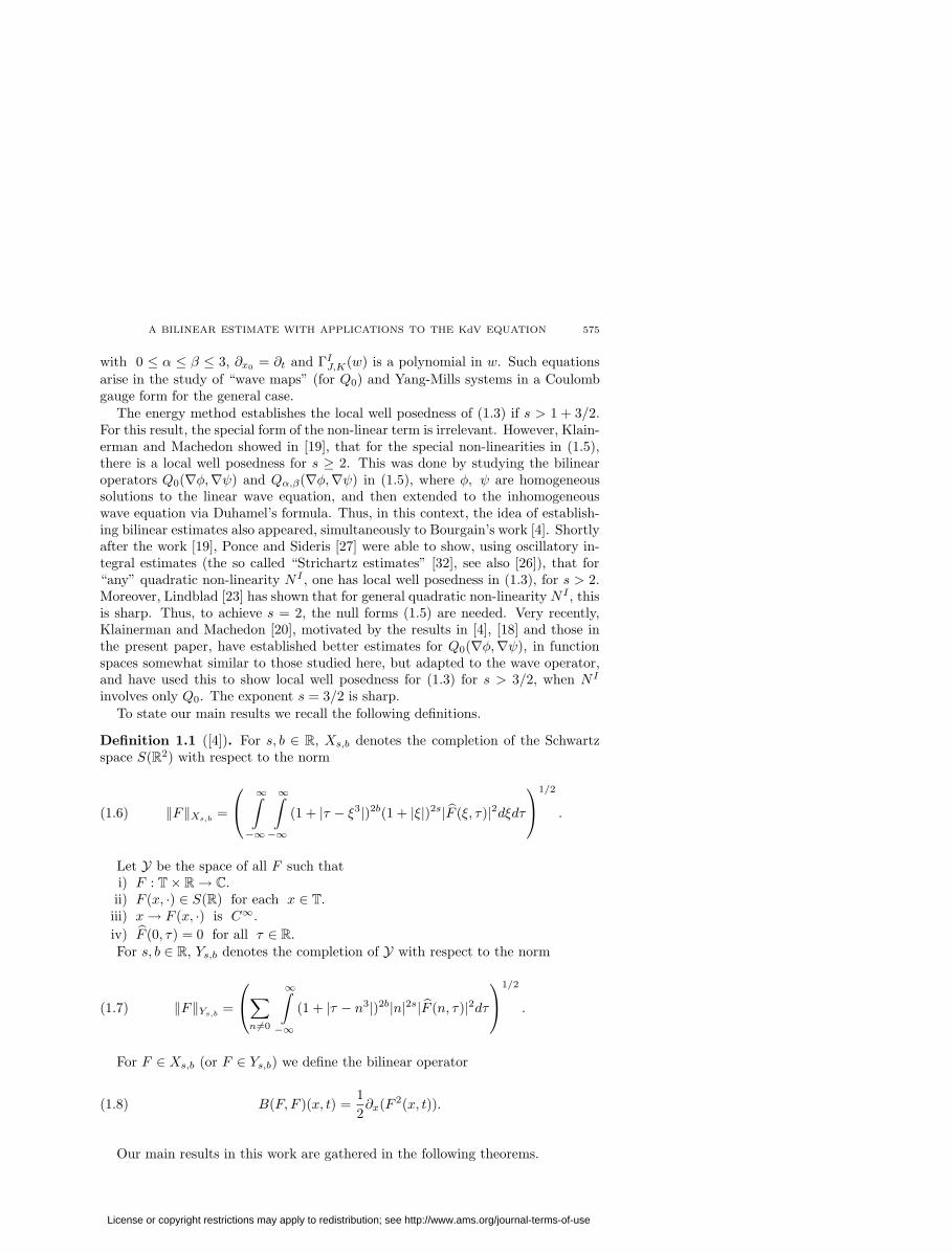
with 0 ≤ α ≤ β ≤ 3, ∂x0 = ∂t and ΓIJ,K(w) is a polynomial in w. Such equations

arise in the study of “wave maps” (for Q0) and Yang-Mills systems in a Coulombgauge form for the general case.

The energy method establishes the local well posedness of (1.3) if s > 1 + 3/2.For this result, the special form of the non-linear term is irrelevant. However, Klain-erman and Machedon showed in [19], that for the special non-linearities in (1.5),there is a local well posedness for s ≥ 2. This was done by studying the bilinearoperators Q0(∇φ,∇ψ) and Qα,β(∇φ,∇ψ) in (1.5), where φ, ψ are homogeneoussolutions to the linear wave equation, and then extended to the inhomogeneouswave equation via Duhamel’s formula. Thus, in this context, the idea of establish-ing bilinear estimates also appeared, simultaneously to Bourgain’s work [4]. Shortlyafter the work [19], Ponce and Sideris [27] were able to show, using oscillatory in-tegral estimates (the so called “Strichartz estimates” [32], see also [26]), that for“any” quadratic non-linearity N I , one has local well posedness in (1.3), for s > 2.Moreover, Lindblad [23] has shown that for general quadratic non-linearity N I , thisis sharp. Thus, to achieve s = 2, the null forms (1.5) are needed. Very recently,Klainerman and Machedon [20], motivated by the results in [4], [18] and those inthe present paper, have established better estimates for Q0(∇φ,∇ψ), in functionspaces somewhat similar to those studied here, but adapted to the wave operator,and have used this to show local well posedness for (1.3) for s > 3/2, when N I

involves only Q0. The exponent s = 3/2 is sharp.To state our main results we recall the following definitions.

Definition 1.1 ([4]). For s, b ∈ R, Xs,b denotes the completion of the Schwartzspace S(R2) with respect to the norm

(1.6) ‖F‖Xs,b =

∞∫−∞

∞∫−∞

(1 + |τ − ξ3|)2b(1 + |ξ|)2s|F (ξ, τ)|2dξdτ

1/2

.

Let Y be the space of all F such thati) F : T× R→ C.ii) F (x, ·) ∈ S(R) for each x ∈ T.iii) x→ F (x, ·) is C∞.

iv) F (0, τ) = 0 for all τ ∈ R.For s, b ∈ R, Ys,b denotes the completion of Y with respect to the norm

(1.7) ‖F‖Ys,b =

∑n6=0

∞∫−∞

(1 + |τ − n3|)2b|n|2s|F (n, τ)|2dτ

1/2

.

For F ∈ Xs,b (or F ∈ Ys,b) we define the bilinear operator

(1.8) B(F, F )(x, t) =1

2∂x(F 2(x, t)).

Our main results in this work are gathered in the following theorems.



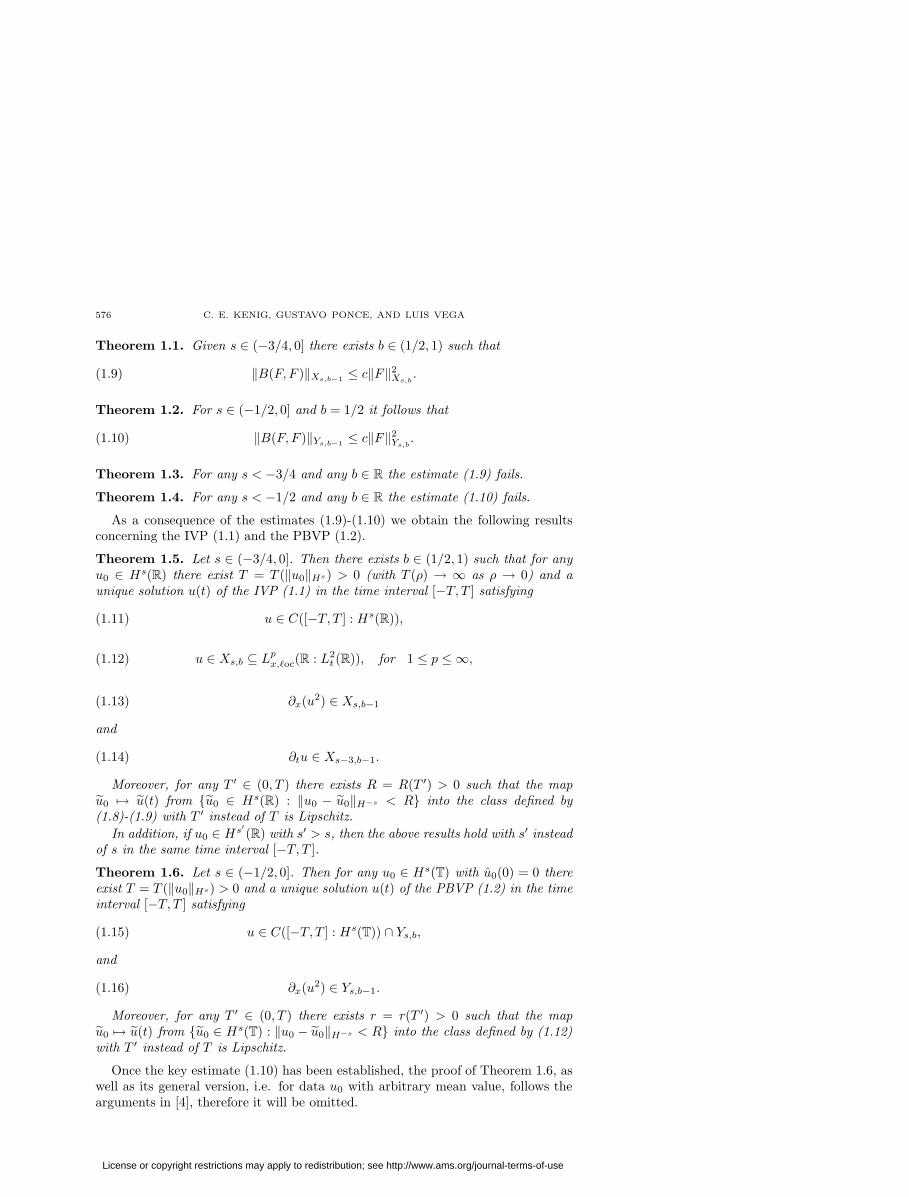
Theorem 1.1. Given s ∈ (−3/4, 0] there exists b ∈ (1/2, 1) such that

(1.9) ‖B(F, F )‖Xs,b−1≤ c‖F‖2Xs,b .

Theorem 1.2. For s ∈ (−1/2, 0] and b = 1/2 it follows that

(1.10) ‖B(F, F )‖Ys,b−1≤ c‖F‖2Ys,b.

Theorem 1.3. For any s < −3/4 and any b ∈ R the estimate (1.9) fails.

Theorem 1.4. For any s < −1/2 and any b ∈ R the estimate (1.10) fails.

As a consequence of the estimates (1.9)-(1.10) we obtain the following resultsconcerning the IVP (1.1) and the PBVP (1.2).

Theorem 1.5. Let s ∈ (−3/4, 0]. Then there exists b ∈ (1/2, 1) such that for anyu0 ∈ Hs(R) there exist T = T (‖u0‖Hs) > 0 (with T (ρ) → ∞ as ρ → 0) and aunique solution u(t) of the IVP (1.1) in the time interval [−T, T ] satisfying

(1.11) u ∈ C([−T, T ] : Hs(R)),

(1.12) u ∈ Xs,b ⊆ Lpx,`oc(R : L2t (R)), for 1 ≤ p ≤ ∞,

(1.13) ∂x(u2) ∈ Xs,b−1

and

(1.14) ∂tu ∈ Xs−3,b−1.

Moreover, for any T ′ ∈ (0, T ) there exists R = R(T ′) > 0 such that the mapu0 7→ u(t) from {u0 ∈ Hs(R) : ‖u0 − u0‖H−s < R} into the class defined by(1.8)-(1.9) with T ′ instead of T is Lipschitz.

In addition, if u0 ∈ Hs′(R) with s′ > s, then the above results hold with s′ insteadof s in the same time interval [−T, T ].

Theorem 1.6. Let s ∈ (−1/2, 0]. Then for any u0 ∈ Hs(T) with u0(0) = 0 thereexist T = T (‖u0‖Hs) > 0 and a unique solution u(t) of the PBVP (1.2) in the timeinterval [−T, T ] satisfying

(1.15) u ∈ C([−T, T ] : Hs(T)) ∩ Ys,b,

and

(1.16) ∂x(u2) ∈ Ys,b−1.

Moreover, for any T ′ ∈ (0, T ) there exists r = r(T ′) > 0 such that the mapu0 7→ u(t) from {u0 ∈ Hs(T) : ‖u0 − u0‖H−s < R} into the class defined by (1.12)with T ′ instead of T is Lipschitz.

Once the key estimate (1.10) has been established, the proof of Theorem 1.6, aswell as its general version, i.e. for data u0 with arbitrary mean value, follows thearguments in [4], therefore it will be omitted.



Theorem 1.5 improves the results in [4], s ≥ 0, and that in [18], s > −5/8.In these works the bounds of the bilinear operator (1.8) in the spaces Xs,b, werebased on several LpLq-estimates, i.e. Strichartz type [32], a sharp version of Katosmoothing effect [13] found in [15], maximal functions and those obtained by inter-polating these. As it was remarked above our proof is elementary. Indeed, it onlyuses simple calculus arguments.

Theorem 1.6 was essentially proven in [4]. There the bound for the bilinearoperator (1.8) was based on the Zygmund result [36] concerning the restriction ofFourier series in L4(T2). As in the continuous case our proof of this key estimateis based on simple calculus inequalities.

It is interesting to compare the above result for the KdV equation with thoseobtained, by different arguments, for the modified KdV (mKdV) equation

(1.17) ∂tv + ∂3xv +

1

3∂x(v3) = 0.

It was proven in [17] that s ≥ 1/4 suffices for the local well posedness of thecorresponding IVP of the mKdV in Hs(R). Similar result, with s > 1/2, for thePBVP associated to (1.14) can be found in [4].

We will show that the method used here does not improve these results. Moreprecisely, let

(1.18) B(F, F, F )(x, t) =1

3∂x(F 3(x, t))

denote the tri-linear operator associated to the mKdV.

Theorem 1.7. For any s < 1/4 and any b ∈ R the estimate

(1.19) ‖B(F, F, F )‖Xs,b−1≤ c‖F‖3Xs,b

fails.

Theorem 1.8. For any s < 1/2 and any b ∈ R the estimate

(1.20) ‖B(F, F, F )‖Ys,b−1≤ c‖F‖3Ys,b

fails.

We observe that in both cases, the IVP and the PBVP, the difference betweenthe best Sobolev exponents known for the local well posedness of the KdV and themKdV is one. Heuristically, this is consistent with the Miura transformation [25]which affirms that if v(·) solves the mKdV (1.14), then

(1.21) u = ci∂xv + v2

solves the KdV equation.For the generalized KdV equation

(1.22) ∂tu+ ∂3xu+

1

k + 1∂x(uk+1) = 0, x, t ∈ R, k ∈ Z+,



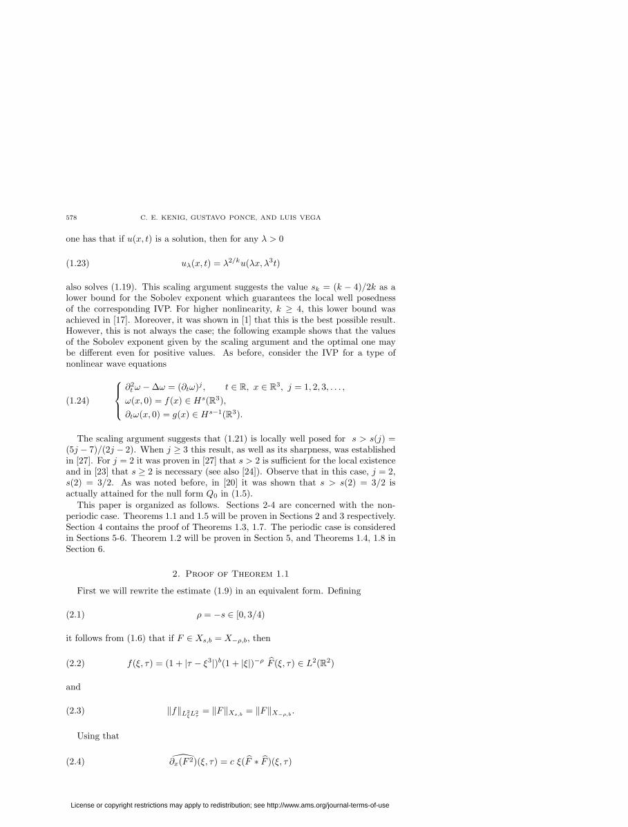
one has that if u(x, t) is a solution, then for any λ > 0

(1.23) uλ(x, t) = λ2/ku(λx, λ3t)

also solves (1.19). This scaling argument suggests the value sk = (k − 4)/2k as alower bound for the Sobolev exponent which guarantees the local well posednessof the corresponding IVP. For higher nonlinearity, k ≥ 4, this lower bound wasachieved in [17]. Moreover, it was shown in [1] that this is the best possible result.However, this is not always the case; the following example shows that the valuesof the Sobolev exponent given by the scaling argument and the optimal one maybe different even for positive values. As before, consider the IVP for a type ofnonlinear wave equations

(1.24)

∂2t ω −∆ω = (∂tω)j , t ∈ R, x ∈ R3, j = 1, 2, 3, . . . ,

ω(x, 0) = f(x) ∈ Hs(R3),

∂tω(x, 0) = g(x) ∈ Hs−1(R3).

The scaling argument suggests that (1.21) is locally well posed for s > s(j) =(5j − 7)/(2j − 2). When j ≥ 3 this result, as well as its sharpness, was establishedin [27]. For j = 2 it was proven in [27] that s > 2 is sufficient for the local existenceand in [23] that s ≥ 2 is necessary (see also [24]). Observe that in this case, j = 2,s(2) = 3/2. As was noted before, in [20] it was shown that s > s(2) = 3/2 isactually attained for the null form Q0 in (1.5).

This paper is organized as follows. Sections 2-4 are concerned with the non-periodic case. Theorems 1.1 and 1.5 will be proven in Sections 2 and 3 respectively.Section 4 contains the proof of Theorems 1.3, 1.7. The periodic case is consideredin Sections 5-6. Theorem 1.2 will be proven in Section 5, and Theorems 1.4, 1.8 inSection 6.

2. Proof of Theorem 1.1

First we will rewrite the estimate (1.9) in an equivalent form. Defining

(2.1) ρ = −s ∈ [0, 3/4)

it follows from (1.6) that if F ∈ Xs,b = X−ρ,b, then

(2.2) f(ξ, τ) = (1 + |τ − ξ3|)b(1 + |ξ|)−ρ F (ξ, τ) ∈ L2(R2)

and

(2.3) ‖f‖L2ξL

2τ

= ‖F‖Xs,b = ‖F‖X−ρ,b .

Using that

(2.4) ∂x(F 2)(ξ, τ) = c ξ(F ∗ F )(ξ, τ)



we can rewrite (1.9) in terms of f as

(2.5)

‖B(F, F )‖Xs,b−1= ‖(1 + |τ − ξ3|)b−1(1 + |ξ|)−ρ ∂x(F 2)‖L2

ξL2τ

= c‖(1 + |ρ− ξ3|)b−1(1 + |ξ|)−ρξ(F ∗ F )‖L2ξL

2τ

= c

∣∣∣∣∣∣∣∣ ξ

(1 + |τ − ξ3|)1−b(1 + |ξ|)ρ ×

∫∫f(ξ1, τ1)(1 + |ξ1|)ρ

(1 + |τ1 − ξ31 |)b

f(ξ − ξ1, τ − τ1)(1 + |ξ − ξ1|)ρdξ1dτ1(1 + |τ − τ1 − (ξ − ξ1)3|)b

∣∣∣∣∣∣∣∣L2ξL

2τ

≤ c‖F‖2Xs,b = c‖f‖2L2ξL

2τ.

Thus, Theorem 1.1 can be restated as follows.

Theorem 2.1. Given ρ = −s ∈ [0, 3/4) there exists b ∈ (1/2, 1) such that

(2.6)

∣∣∣∣∣∣∣∣ ξ

(1 + |τ − ξ3|)1−b(1 + |ξ|)ρ×

∫∫f(ξ1, τ1)(1 + |ξ1|)ρ

(1 + |τ1 − ξ31 |)b

f(ξ − ξ1, τ − τ1)(1 + |ξ − ξ1|)ρ(1 + |τ − τ1 − (ξ − ξ1)3|)b dξ1dτ1

∣∣∣∣∣∣∣∣L2ξL

2τ

≤ c‖f‖2L2ξL

2τ.

We will restrict ourselves to the most interesting cases of (2.6), ρ = 0, whichprovides a simplified proof of the L2-result in [4], and ρ ∈ (1/2, 3/4). In fact wewill prove the following slightly stronger version of Theorem 2.1.

Theorem 2.2. Given ρ = −s ∈ (1/2, 3/4) there exists b ∈ (1/2, 1) such that forany b′ ∈ (1/2, b] with b− b′ ≤ min{ρ− 1/2; 1/4− ρ/3} it follows that

(2.7)

∣∣∣∣∣∣∣∣ ξ

(1 + |τ − ξ3|)1−b(1 + |ξ|)ρ×

∫∫f(ξ1, τ1)(1 + |ξ1|)ρ

(1 + |τ1 − ξ31 |)b

′f(ξ − ξ1, τ − τ1)(1 + |ξ − ξ1|)ρ

(1 + |τ − τ1 − (ξ − ξ1)3|)b′ dξ1dτ1

∣∣∣∣∣∣∣∣L2ξL

2τ

≤ c‖f‖2L2ξL

2τ,

where the constant c depends on ρ, b and b− b′.Moreover (2.7) still holds for ρ = 0, b ∈ (1/2, 3/4] and b′ ∈ (1/2, b].

We observe that (2.6) follows from (2.7) by taking b′ = b.The following elementary calculus inequalities will provide the main tool in the

proof of Theorem 2.2.



Lemma 2.3. If ` > 1/2, then there exists c > 0 such that

(2.8)

∞∫−∞

dx

(1 + |x− α|)2`(1 + |x− β|)2`≤ c

(1 + |α− β|)2`,

(2.9)

∞∫−∞

dx

(1 + |x|)2`|√α− x |

≤ c

(1 + |α|)1/2,

(2.10)

∞∫−∞

dx

(1 + |x− α|)2(1−`)(1 + |x− β|)2`≤ c

(1 + |α− β|)2(1−`)

and

(2.11)

∫|x|≤β

dx

(1 + |x|)2(1−`)|√α− x |

≤ c (1 + β)2(`−1/2)

(1 + |α|)1/2.

Next, using these calculus inequalities, we deduce three lemmas from which theproof of Theorem 2.2 will follow directly.

Lemma 2.4. If b ∈ (1/2, 3/4] and b′ ∈ (1/2, b], then there exists c > 0 such that

(2.12)

|ξ|(1 + |τ − ξ3|)1−b × ∞∫

−∞

∞∫−∞

dτ1dξ1(1 + |τ1 − ξ3

1 |)2b′(1 + |τ − τ1 − (ξ − ξ1)3|)2b′

1/2

≤ c.

Proof. Since b′ > 1/2, from (2.8) it follows that

(2.13)

∞∫−∞

dτ1(1 + |τ1 − ξ3

1 |)2b′(1 + |τ − τ1 − (ξ − ξ1)3|)2b′

≤ c

(1 + |τ − ξ3 + 3ξξ1(ξ − ξ1)|2b′) .

To integrate with respect to ξ1 we change variables

(2.14) µ = λ− ξ3 + 3ξξ1(ξ − ξ1), then dµ = 3ξ(ξ − 2ξ1)dξ1,

and

(2.15) ξ1 =1

2

{ξ ±

√4τ − ξ3 − 4µ

3ξ

}.



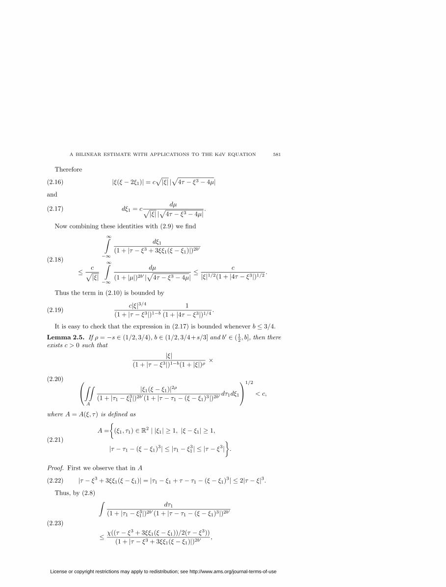
Therefore

(2.16) |ξ(ξ − 2ξ1)| = c√|ξ| |√

4τ − ξ3 − 4µ|

and

(2.17) dξ1 = cdµ√

|ξ| |√

4τ − ξ3 − 4µ|.

Now combining these identities with (2.9) we find

(2.18)

∞∫−∞

dξ1(1 + |τ − ξ3 + 3ξξ1(ξ − ξ1)|)2b′

≤ c√|ξ|

∞∫−∞

dµ

(1 + |µ|)2b′ |√

4τ − ξ3 − 4µ|≤ c

|ξ|1/2(1 + |4τ − ξ3|)1/2.

Thus the term in (2.10) is bounded by

(2.19)c|ξ|3/4

(1 + |τ − ξ3|)1−b1

(1 + |4τ − ξ3|)1/4.

It is easy to check that the expression in (2.17) is bounded whenever b ≤ 3/4.

Lemma 2.5. If ρ = −s ∈ (1/2, 3/4), b ∈ (1/2, 3/4+s/3] and b′ ∈ (12 , b], then there

exists c > 0 such that

(2.20)

|ξ|(1 + |τ − ξ3|)1−b(1 + |ξ|)ρ ×

∫∫A

|ξ1(ξ − ξ1)|2ρ(1 + |τ1 − ξ3

1 |)2b′(1 + |τ − τ1 − (ξ − ξ1)3|)2b′dτ1dξ1

1/2

< c,

where A = A(ξ, τ) is defined as

(2.21)

A =

{(ξ1, τ1) ∈ R2 | |ξ1| ≥ 1, |ξ − ξ1| ≥ 1,

|τ − τ1 − (ξ − ξ1)3| ≤ |τ1 − ξ31 | ≤ |τ − ξ3|

}.

Proof. First we observe that in A

(2.22) |τ − ξ3 + 3ξξ1(ξ − ξ1)| = |τ1 − ξ1 + τ − τ1 − (ξ − ξ1)3| ≤ 2|τ − ξ|3.

Thus, by (2.8)

(2.23)

∫dτ1

(1 + |τ1 − ξ31 |)2b′(1 + |τ − τ1 − (ξ − ξ1)3|)2b′

≤ χ((τ − ξ3 + 3ξξ1(ξ − ξ1))/2(τ − ξ3))

(1 + |τ − ξ3 + 3ξξ1(ξ − ξ1)|)2b′,



where χ(·) denotes the characteristic function of the interval [−1, 1].As in the previous Lemma we use the change of variable

(2.24) µ = τ − ξ3 + 3ξξ1(ξ − ξ1).

Thus (2.14)-(2.17), (2.23) and (2.29) lead to the inequalities

(2.25)

∫∫A

|ξ1(ξ − ξ1)|2ρ(1 + |τ1 − ξ3

1 |)2b′(1 + |τ − τ1 − (ξ − ξ1)3|)2b′dξ1dτ1

≤ c∫ |ξ1(ξ − ξ1)|2ρχ((τ − ξ3 + 3ξξ1(ξ − ξ1))/2(τ − ξ3))

(1 + |τ − ξ3 + 3ξξ1(ξ − ξ1)|)2b′dξ1

≤ c∫

|µ|≤2|τ−ξ3|

|τ − ξ3 − µ|2ρ

|ξ|2ρ+1/2(1 + |µ|)2b′ |√

4τ − ξ3 − 4µ|dµ

≤ c

|ξ|2ρ+1/2

|τ − ξ3|2ρ(1 + |4τ − ξ3|)1/2

.

Hence the expression

(2.26) φ(ξ, τ) =c|ξ|3/4−ρ(1 + |ξ|)ρ

(1 + |τ − ξ3|)ρ+b−1

(1 + |4τ − ξ3|)1/4

bounds the term in (2.20). From the assumptions on ρ = −s and b one has that

(2.27) φ ∈ L∞(R2),

which completes the proof.

Lemma 2.6. If ρ = −s ∈ (1/2, 3/4), b ∈ (1/2, 1) and b′ ∈ (1/2, b] with b − b′ ≤min{ρ− 1/2; 1/4− ρ/3}, then there exists c > 0 such that

(2.28)

1

(1 + |τ1 − ξ31 |)b

′ ×

∫∫B

|ξ|2(1−ρ)|ξξ1(ξ − ξ1)|2ρ dτdξ(1 + |ξ|)2ρ(1 + |τ − ξ3|)2(1−b)(1 + |τ − τ1 − (ξ − ξ1)3|)2b′

1/2

≤ c,

where B = B(ξ1, τ1) is defined as

(2.29)

B =

{(ξ, τ) ∈ R2

∣∣ |ξ − ξ1| ≥ 1, |ξ1| ≥ 1,

|τ − τ1 − (ξ − ξ1)3| ≤ |τ1 − ξ31 |, |τ − ξ3| ≤ |τ1 − ξ3

1 |}.



Proof. First we observe that in B

(2.30) |τ1 − ξ31 + 3ξξ1(ξ − ξ1)| = |τ − ξ3 − (τ − τ1 − (ξ − ξ1)3)| ≤ 2|τ1 − ξ3

1 |.

By (2.10) it follows that

(2.31)

∫dτ

(1 + |τ − ξ3|)2(1−b)(1 + |τ − τ1 − (ξ − ξ1)3|)2b′

≤ c

(1 + |τ1 − ξ31 + 3ξξ1(ξ − ξ1)|)2(1−b) .

Thus to obtain (2.28) it suffices to bound

(2.32)

I(D) =1

(1 + |τ1 − ξ31 |)b

′ × ∫D

|ξ|2(1−ρ)|ξξ1(ξ − ξ1)|2ρ(1 + |ξ|)2ρ(1 + |τ1 − ξ3

1 + 3ξξ1(ξ − ξ1)|)2(1−b) dξ

1/2

with D = B′ = B′(ξ1, τ1), where

(2.33)

B′ =

{ξ ∈ R

∣∣ 1 ≤ |ξ − ξ1|, 1 ≤ |ξ1|, |τ − ξ3| ≤ |τ1 − ξ31 |

|τ1 − ξ31 + 3ξξ1(ξ − ξ1)| ≤ 2|τ1 − ξ3

1 |}.

We split B′ into two subdomains B′1 and B′2, where

(2.34) B′1 =

{ξ ∈ B′

∣∣ 3|ξξ1(ξ − ξ1)| ≤ 1

2|τ1 − ξ3

1 |}

and

(2.35) B′2 =

{ξ ∈ B′

∣∣ 1

2|τ1 − ξ3

1 | ≤ 3|ξξ1(ξ − ξ1)| ≤ 3|τ1 − ξ31 |}.

In B′1 we have that

(2.36)1

2|τ1 − ξ3

1 | ≤ |τ1 − ξ31 + 3ξξ1(ξ − ξ1)|

and

(2.37) |ξ| ≤ 1

6|τ1 − ξ3

1 |.

Hence

(2.38)I(B′1) ≤ c

(1 + |τ1 − ξ31 |)1−ρ+b′−b

∫|ξ|≤|τ1−ξ3

1 |

|ξ|2(1−ρ)

(1 + |ξ|)2ρdξ

1/2

≤ c(1 + |τ1 − ξ31 |)1/2−ρ−b′+b

which is bounded since, by hypothesis, 1/2− ρ− b′ + b ≤ 0.



To bound I(B′2) we split B′2 into three parts, B′2,1, B′2,2 and B′2,3.First we have

(2.39) B′2,1 =

{ξ ∈ B′2

∣∣ 1

4|ξ| ≤ |ξ1| ≤ 100|ξ|

}.

In this domain one has

(2.40) c(1 + |τ1 − ξ31 |) ≤ |ξ1|3 ∼ |ξ|3.

Combining (2.35), the hypothesis ρ > 1/2, a change of variable similar to thatin (2.14)-(2.17), µ1 = τ1 − ξ3

1 + 3ξξ1(ξ − ξ1), and (2.9) it follows that

(2.41)

I(B′2,1) ≤ c(1 + |τ1 − ξ31 |)ρ−b

′+(1−2s)/3× ∫|µ1|≤2|τ1−ξ3

1 |

dξ

(1 + |τ1 − ξ31 + 3ξξ1(ξ − ξ1)|)2(1−b)

1/2

≤ c(1 + |τ1 − ξ31 |)ρ/3−b

′+1/3 × 1

|ξ|1/4∫

|µ1|<2|τ1−ξ31|

1

(1 + |µ1|)2(1−b)dµ1∣∣ √4τ1 − ξ3

1 − 4µ1

∣∣

1/2

≤ c (1 + |τ1 − ξ31 |)ρ/3−1/4+b−b′

(1 + |4τ1 − ξ31 |)1/4

,

which is bounded since, by hypothesis, ρ/3− 1/4 + b− b′ ≤ 0.Next we consider

(2.42) B′2,2 =

{ξ ∈ B′2

∣∣ 1 ≤ |ξ1| ≤ |ξ|/4}.

In this domain one has that

(2.43) |ξ1 − 2ξ| ∼ |ξ| ∼ |ξ − ξ1|

and

(2.44) c−1(1 + |τ1 − ξ31 |) ≤ |ξξ1(ξ − ξ1)| ∼ |ξ|2|ξ1| ≤ c|ξ|3.

Therefore (2.44), the change of variable µ1 = λ1 − ξ31 + 3ξξ1(ξ − ξ1) and (2.11)

give the inequalities

(2.45 )

I(B′2,2) ≤ c

(1 + |τ1 − ξ31 |)b

′ × ∫|µ1|≤3|τ1−ξ3

1 |

|ξ|2(1−2ρ)|ξξ1(ξ − ξ1)|2ρ|ξ1|1/2(1 + |τ1 − ξ3

1 |)1/2(1 + |µ1|)2(1−b) dµ1

1/2

≤ c(1 + |τ1 − ξ31 |)θ,



where

(2.46) θ = −b′ + 1/4 + (1− 2ρ)/3 + ρ+ b− 1/2 = ρ/3− 5/12 + b− b′ ≤ 0

by using our hypothesis on ρ, b and b′. Hence I(B′2,2) is bounded.Finally we have

(2.47) B′2,3 =

{ξ ∈ B′2

∣∣ 100|ξ| ≤ |ξ1|}.

In this case one has that

(2.48) |ξ1 − 2ξ| ∼ |ξ1 − ξ| ∼ |ξ1|, |τ1 − ξ31 | << |ξ1|3

and

(2.49) |4τ1 − ξ31 | ∼ |ξ3

1 |.

Thus a familiar argument shows that

(2.50)

I(B′2,3) ≤ c(1 + |τ1 − ξ31 |)ρ−b

′ × 1

|ξ1|1/2∫

|µ1|≤3|τ1−ξ31 |

1

(1 + |µ1|)2(1−b)dµ1∣∣√4τ1 − ξ3

1 − 4µ1

∣∣

1/2

≤ c(1 + |τ1 − ξ31 |)ρ−5/6−b′+b,

which is bounded. This completes the proof of (2.28).

Proof of Theorem 2.2. First we consider the case s = 0. Using Cauchy-Schwarzinequality, (2.12) and Fubini’s theorem it follows that

(2.51)

∥∥∥∥ ξ

(1 + |τ − ξ3|)1−b

∫∫f(ξ1, τ1)

(1 + |τ1 − ξ31 |)b

′f(ξ − ξ1, τ − τ1)dξ1dτ1

(1 + |τ − τ1 − (ξ − ξ1)3|)b′∥∥∥∥L2ξL

2τ

≤∥∥∥∥ ξ

(1 + |τ − ξ3|)1−b×(∫∫dξ1dτ1

(1 + |τ1 − ξ31 |)2b′(1 + |τ − τ1 − (ξ − ξ1)3|)2b′

)1/2∥∥∥∥∥L∞ξ L

∞τ∥∥∥∥∥

(∫∫|f(ξ1, τ1)|2 |f(ξ − ξ1, τ − τ1)|2 dξ1dτ1

)1/2∥∥∥∥∥L2ξL

2τ

≤ c‖f‖2L2ξL

2τ,

for any b′ ∈ (1/2, b]. Taking b′ = b we obtain the result.Next we turn to the case ρ = −s ∈ (1/2, 3/4). Note that if

(2.52) either |ξ1| ≤ 1 or |ξ − ξ1| ≤ 1,



we have

(2.53) (1 + |ξ1|)ρ(1 + |ξ − ξ1|)ρ ≤ c(1 + |ξ|)ρ,

which reduces the estimate to the case ρ = 0. Thus, we can assume

(2.54) |ξ1| ≥ 1 and |ξ − ξ1| ≥ 1.

By symmetry we can also assume

(2.55) |τ − τ1 − (ξ − ξ1)3| ≤ |τ1 − ξ31 |.

We split the region of integration in (2.7) into two parts

(2.56) |τ1 − ξ31 | ≤ |τ − ξ3| and |τ − ξ3| ≤ |τ1 − ξ3

1 |.

For the first part we use Cauchy-Schwarz and (2.20) as in (2.51) to obtain thesame bound. For the second part we use duality, Cauchy-Schwarz and (2.28) toconclude the proof.

We observe that Theorem 2.2 is equivalent to the following result.

Corollary 2.7. Given s ∈ (−3/4,−1/2) there exists b ∈ (1/2, 1) such that for anyb′ ∈ (1/2, b] with b− b′ ≤ min{−s− 1/2; 1/4 + s/3}

(2.57) ‖B(F, F )‖Xs,b−1≤ c‖F‖2Xs,b′ .

Moreover (2.57) still holds for s = 0, b ∈ (1/2, 3/4] and b′ ∈ (1/2, b].


We will denote by {W (t)}∞−∞ the unitary group describing the solution of thelinear IVP associated to (1.1):

(3.1)

{∂tu+ ∂3

xu = 0, t, x ∈ R,u(x, 0) = u0(x),

where

(3.2) u(x, t) = W (t)u0(x) = St ∗ u0(x)

with St(·) defined by the oscillatory integral

(3.3) St(x) = c

∞∫−∞

eixξeitξ3

dξ.

We will also use the notation

(3.4) ‖f‖LpxLqt =

∞∫−∞

∞∫−∞

|f(x, t)|qdt

p/q

dx

1/q

,



(3.5) Jsh(ξ) = (1 + |ξ|)s h(ξ) , Dsxh(ξ) = |ξ|s h(ξ)

and

(3.6) Λbg(τ) = (1 + |τ |)b g(τ) , Dbtg(τ) = |τ |b g(τ).

The relationship between the spaces Xs,b in (1.6) and the group {W (t)}∞−∞ in(3.2) is described by the identity

(3.7) ‖F‖Xs,b = ‖ΛbJsW (t)F‖L2ξL

2τ.

Hence, if F ∈ Xs,b then

(3.8)F = F (x, t) =

((1 + |ξ|)−s(1 + |τ − ξ3|)−b f(ξ, τ)

)∨=(

(1 + |ξ|)−s fb(ξ, τ))∨

with f ∈ L2(R2). From the sharp version of the Kato smoothing effect [13] foundin [15], i.e.

(3.9) ‖DxW (t)v0‖L∞x L2t≤ c‖v0‖L2,

it follows that for b > 1/2

(3.10) Dθxfb ∈ L2/(1−θ)

x L2t , for θ ∈ [0, 1].

In particular, this implies that for s ∈ (−1, 0)

(3.11) F ∈ Cα`oc(R : L2t (R)) with α ∈ (0, 1 + s).

Lemma 3.1. If F ∈ Xs,b with s ∈ (−1, 0) and b > 1/2, then

(3.12) F ∈ Cα`oc(R : L2t (R)) ⊆ Lpx,loc(R : L2

t (R))

for 1 ≤ p ≤ ∞, and α ∈ (0, 1 + s).

Let ψ ∈ C∞0 (R) with ψ ≡ 1 on [−1, 1] and supp ψ ⊆ (−2, 2). We recall thefollowing results proven in [18].

Lemma 3.2. If s ≤ 0 and b ∈ (1/2, 1], then for δ ∈ (0, 1)

(3.13) ‖ψ(δ−1t)W (t)v0‖Xs,b ≤ c δ(1−2b)/2‖v0‖Hs ,

(3.14) ‖ψ(δ−1t)F‖Xs,b ≤ c δ(1−2b)/2‖F‖Xs,b,

(3.15)

∥∥∥∥∥∥ψ(δ−1t)

t∫0

W (t− t′)F (t′)dt′

∥∥∥∥∥∥Xs,b

≤ c δ(1−2b)/2‖F‖Xs,b−1



and

(3.16)

∥∥∥∥∥∥ψ(δ−1t)

t∫0

W (t− t′)F (t′)dt′

∥∥∥∥∥∥Hs

≤ c δ(1−2b)/2‖F‖Xs,b−1.

Proof. For (3.13)-(3.15) see Lemmas 3.1-3.3 in [18]. The proof of (3.16) follows thesame argument used in [18] to obtain (3.15).

Proof of Theorem 1.5. First we observe that if u(·) is a solution of the IVP (1.1),then for any λ > 0

(3.17) uλ(x, t) = λ2u(λx, λ3t)

also satisfies the KdV equation with data

(3.18) uλ(x, 0) = λ2u0(λx).

Thus for s ≤ 0

(3.19) ‖uλ(·, 0)‖Hs = 0(λ3/2+s) as λ→ 0.

In our case s ∈ (−3/4, 0], hence, without loss of generality, we can restrict ourselvesto considering the IVP (1.1) with data u0(x) satisfying

(3.20) ‖u0‖Hs = r << 1,

i.e., r arbitrary small; see (3.24) below.For u0 ∈ Hs(R), s ∈ (−3/4, 0], satisfying (3.20) we define the operator

(3.21) Φu0(ω) = Φ(ω) = ψ(t)W (t)u0 −ψ(t)

2

t∫0

W (t− t′)ψ2(t′)∂x(ω2(t′))dt′.

We shall prove that Φ(·) defines a contraction on

(3.22) B(2c r) =

{ω ∈ Xs,b | ‖ω‖Xs,b ≤ 2c r

}.

First combining (3.13)-(3.15) and (1.9) (Theorem 1.1) it follows that for ω ∈ B2cr

(3.23)‖Φ(ω)‖Xs,b ≤ cr + c‖∂x(ψ(t)ω(·, t))2‖Xs,b−1

≤ cr + c‖ψω‖2Xs,b≤ cr + c‖ω‖2Xs,b ≤ cr + c(2cr)2 ≤ 2cr

for r in (3.20) satisfying

(3.24) 4c2r ≤ 1.



Similarly using (3.14)-(3.15), (1.9) and (3.24) it follows that for ω, ω ∈ B(2cr)

(3.25)

‖Φ(ω)− Φ(ω)‖Xs,b

=1

2

∥∥∥∥∥∥ψ(t)

t∫0

W (t− t′)ψ2(t′) ∂x(ω2 − ω2)(t′)dt′

∥∥∥∥∥∥Xs,b

≤ c‖ω + ω‖Xs,b‖ω − ω‖Xs,b ≤ 2c2r ‖ω − ω‖Xs,b

≤ 1

2‖ω − ω‖Xs,b .

Thus Φ(·) is a contraction. Therefore there exists a unique u ∈ B(2cr) such that

(3.26) u(t) = ψ(t)

W (t)u0 −1

2

t∫0

W (t− t′)∂x(ψ(t′)u(t′))2dt′

.

Hence, in the time interval [−1, 1], u(·) solves the integral equation associated tothe IVP (1.1).

Now we turn to the proof of the persistence property, i.e.

(3.27) u ∈ C([−1, 1] : Hs(R))

and the continuous dependence of the solution upon the data in the norm of thespace in (3.27). Combining (3.7) and Holder and Sobolev inequalities we obtain

(3.28)

‖ψ(ρ−1·)u‖Xs,0 = ‖Js(ψ(ρ−1·)u)‖L2tL

2x

= ‖W (t)(ψ(ρ−1·)Jsu)‖L2tL

2x

= ‖ψ(ρ−1·)W (t)Jsu‖L2xL

2t

≤ cρ1/4‖ψ(ρ−1·)W (t)Jsu‖L2xL

4t

≤ cρ1/4‖D1/4t (ψ(ρ−1·)W (t)Jsu)‖L2

xL2t

= cρ1/4‖ψ(ρ−1·)u‖Xs,1/2

≤ cρ1/4‖ψ(ρ−1·)u‖Xs,b .

Thus, by Holder’s inequality, (3.14) and (3.28), for 0 < b ≤ b′ we find that

(3.29)

‖ψ(ρ−1·)u‖Xs,b′ ≤ ‖ψ(ρ−1·)u‖(b−b′)/2

Xs,0‖ψ(ρ−1·)u‖b

′/bXs,b

≤ c ρ(b−b′)/8‖ψ(ρ−1·

)u‖Xs,b ≤ c ρ(b−b′)/8∣∣∣∣u∣∣∣∣

Xs,b.

Using the integral equation (3.26), (2.57) with some fixed b′ < b, (3.14), (3.16)



and (3.29), for 0 ≤ t < t ≤ 1 and t− t ≤ ∆t it follows that

(3.30)

‖u(t)− u(t)‖Hs ≤ ‖W (t− t)u(t)− u(t)‖Hs

+ c

∥∥∥∥∥∥t∫t

W (t− t′)ψ2

(t′ − t∆t

)∂x(u2(t′))dt′

∥∥∥∥∥∥Hs

≤ ‖W (t− t)u(t)− u(t)‖Hs + c

∥∥∥∥∂x(ψ2

(· − t∆t

)u2

)∥∥∥∥Xs,b−1

≤ ‖W (t− t)u(t)− u(t)‖Hs + c

∥∥∥∥ψ( · − t∆t

)u

∥∥∥∥2

Xs,b′

≤ ‖W (t− t)u(t)− u(t)‖Hs + c(∆t)(b−b′)/4‖u‖2Xs,b = o(1)

as ∆t → 0, which yields the persistence property. The proof of the continuousdependence of the solution upon the data in the L∞([0, 1] : Hs(R))-norm follows asimilar argument, therefore it will be omitted.

Finally we explain how to extend the uniqueness result in B(2cr) in (3.22) to thewhole Xs,b. For any δ ∈ (0, 1) we define

(3.31) B(2cδ(1−2b)/2r) =

{ω ∈ Xs,b

∣∣ ‖ω‖Xs,b ≤ 2cδ(1−2b)/2r

}and(3.32)

Φδ,u0(ω) = Φδ(ω) = ψ(δ−1t)W (t)u0 −ψ(δ−1t)

2

t∫0

W (t− t′)ψ2(t′)∂x(ω2(t′))dt′.

Combining (2.57) with b′ ∈ (12 , b) such that

(3.33) b− b′ = min{−s− 1/2; 1/4 + s/3}

with the arguments in (3.23) and (3.29) one has

(3.34) ‖Φδ(ω)‖Xs,b ≤ c δ(1−2b)/2r + 4c3δ3(1−2b)/2δ(b−b′)/4r2,

and

(3.35) ‖Φδ(ω)− Φδ(ω)‖Xs,b ≤ 2c3δ(1−2b)δ(b−b′)/4r‖ω − ω‖Xs,b .

By (3.33) it follows that

(3.36) 1− 2b+ (b− b′)/4 < 0,

therefore for any δ ∈ (0, 1)

(3.37) Φδ(B(2cδ(1−2b)/2r)) ⊆ B(2cδ(1−2b)/2r)

is a contraction, which completes the proof.



4. Proof of Theorems 1.3 and 1.7

Proof of Theorem 1.3. Using the notation in (2.1)-(2.5), one sees that (1.9) is equiv-alent to

(4.1)

∣∣∣∣∣∣∣∣ ξ

(1 + |τ − ξ3|)1−b(1 + |ξ|)ρ ×

∫∫f(ξ1, τ1)(1 + |ξ1|)ρ

(1 + |τ1 − ξ31 |)b

f(ξ − ξ1, τ − τ1)(1 + |ξ − ξ1|)ρdξ1dτ1(1 + |τ − τ1 − (ξ − ξ1)3|)b

∣∣∣∣∣∣∣∣L2ξL

2τ

≤ c ‖f‖2L2ξL

2τ.

First we shall see that if ρ = −s > 3/4, then b ≤ 1/2.Fix N ∈ Z+ and take

(4.2) f(ξ, τ) = χA

(ξ, τ) + χ−A(ξ, τ),

where χA

(·) represents the characteristic function of the set A with

(4.3) A =

{(ξ, τ) ∈ R2

∣∣ N ≤ ξ ≤ N +1√N, |τ − ξ3| ≤ 1

}and

(4.4) −A =

{(ξ, τ) ∈ R2| − (ξ, τ) ∈ A

}.

Clearly

(4.5) ‖f‖L2ξL

2τ≤ c N− 1

4 .

On the other hand, A contains a rectangle with (N,N3) as a vertex, with di-mensions 10−2N−2 ×N3/2 and longest side pointing in the (1, 3N2) direction.

Therefore

(4.6) |(f ∗ f)(ξ, τ)| ≥ c√NχR(ξ, τ),

where R is the rectangle centered at the origin of dimensions cN−2 × N32 and

longest side pointing in the (1, 3N2) direction. Hence (4.1) implies that

(4.7) N2ρN−12N

32 (b−1)N−

12N

14 ≤ c N− 1

2 ,

i.e.

(4.8) b+ 4ρ ≤ 3

2

as desired.



To complete the proof we just need to show that if ρ = −s > 3/4 then b > 1/2.By polarization and duality (4.1) is equivalent to the following inequality:

(4.9)

∣∣∣∣∣∣∣∣ (1 + |ξ1|)ρ(1 + |τ1 − ξ3

1 |)b×

∫∫ |ξ|(1 + |ξ|)s

g(ξ, τ)

(1 + |τ − ξ3|)1−bh(ξ − ξ1, τ − τ1)(1 + |ξ − ξ1|)s

(1 + |τ − τ1 − (ξ − ξ1)3|)b dξdτ

∣∣∣∣∣∣∣∣L2ξ1L2τ1

≤ c ‖g‖L2ξL

2τ‖h‖L2

ξL2τ.

We take

(4.10) g(ξ, τ) = χA

(ξ, τ), (A defined in (4.3))

and

(4.11) h(ξ, τ) = χB (ξ, τ),

where

(4.12) B =

{(ξ, τ) ∈ R2 | −N + 1/2

√N ≤ ξ ≤ −N + 3/4

√N ; |τ − ξ3| < 1

}.

Estimating the first norm in (4.9) in the domain

(4.13) |4τ1 − ξ31 | ≤

1

4and ξ1 ∈

[N − 1

20

1√N, N − 1

10

1√N

]from (4.9) we see that

(4.14)Nρ+1/4

N3b≤ N−1/2,

i.e. if ρ = −s > 3/4

(4.15)3

2< ρ+

3

4≤ 3b.

Proof of Theorem 1.7. We consider the case b = 1/2, and remark that a similarargument to that used in the previous proof shows that this assumption does notimply a loss of generality.

First we take F (·, ·) such that

(4.16) F (ξ, τ) = χA(ξ, τ) + χ−A(ξ, τ),

where A was defined in (4.3). Thus

(4.17)∣∣(F ∗ F ∗ F )(ξ, τ)

∣∣ ≥ c√N

∣∣(χA∗ χR)(ξ, τ)

∣∣,



where R represents the rectangle centered at the origin of dimension 10−2N−2 ×N3/2 and with its longest side pointing in the (1, 3N2) direction.

Then

(4.18)∣∣(F ∗ F ∗ F )(ξ, τ)

∣∣ ≥ c

NχR0

(ξ, τ),

where R0 is a rectangle like R, of the same dimensions and direction, but with(N,N3) as one of its vertices. Hence

(4.19) ‖B(F, F, F )‖Xs,b−1≥ cNs−1/4.

Since

(4.20) ‖F‖Xs,b ≤ cNs−1/4,

(1.18) implies that s ≥ 1/4, which completes the proof.


First we rewrite the inequality (1.10). Defining

(5.1) ρ = −s ∈ [0, 1/2)

by (1.7) it follows that if F ∈ Ys,b = Y−ρ,b, then

(5.2) f(n, τ) = (1 + |τ − n3|)b|n|−ρF (n, τ) ∈ L2τ (R : `2n(T))

and

(5.3) ‖f‖L2τ`

2n

= ‖F‖Y−ρ,b .

Since

(5.4) ∂x(F 2)(n, τ) = c n (F ∗ F )(n, τ)

we can express (1.10) in terms of f as

(5.5)

‖B(F, F )‖Ys,b−1,0= ‖(1 + |τ − n3|)b−1|n|−ρ∂x(F 2)(n, τ)‖L2

τ `2n

= c ‖(1 + |τ − n3|)b−1|n|−ρn(F ∗ F )(n, τ)‖L2τ `

2n

=

(∑n6=0

∞∫−∞

|n|2(1 + |τ − n3|)2(1−b)|n|2ρ×∣∣∣∣ ∑

n1 6=nn1 6=0

∞∫−∞

|n1(n− n1)|ρ(1 + |τ1 − n3

1|)1/2×

f(n1, τ1)

(1 + |τ1 − n31|)1/2

f(n− n1, τ − τ1)dτ1(1 + |τ − τ1 − (n− n1)3|)1/2

∣∣∣∣2)1/2

= ‖B(f, f)(n, τ)‖L2τ`

2n≤ c(∑n6=0

∞∫−∞

|f(n, τ)|2dτ)

= c‖f‖2L2τ`

2n.

As in the continuous case we first need some calculus results.



Lemma 5.1. There exists c > 0 such that for any n 6= 0 and any τ ∈ R

(5.6)∑n1 6=0n1 6=n

log(2 + |τ − nn1(n− n1)|)1 + |τ − nn1(n− n1)| < c.

Proof. Since n 6= 0 it suffices to show that

(5.7)

∣∣∣∣∣∣∣∣ ∑n1 6=0n1 6=n

1

(1 + |µ− n1(n− n1)|)3/4

∣∣∣∣∣∣∣∣L∞µ `

∞n

< c.

Let α, β be the roots of the equation

(5.8) µ− n1(n− n1) = 0,

i.e.

(5.9) µ− n1(n− n1) = (n1 − α)(n1 − β), with α = α(n, µ), β = β(n, µ).

We shall prove that

(5.10)

∣∣∣∣∣∣∣∣∑n1

1

(1 + |(n1 − α)(n1 − β)|)3/4

∣∣∣∣∣∣∣∣L∞α L

∞β

< c,

which implies (5.7).

Notice that for a fixed (α, β) ∈ R2 there exist at most 8 n1’s such that

(5.11) |n1 − α| ≤ 2 or |n1 − β| ≤ 2.

For the remaining n1’s one has that

(5.12) 1 + |n1 − α| |n1 − β| ≥1

2(1 + |n1 − α|)(1 + |n1 − β|),

hence∑n1

1

(1 + |(n1 − α)(n1 − β)|)3/4≤ 8 +

∑|n1−α|≥2

|n1−β|≥2

1

(1 + |(n1 − α)(n1 − β)|)3/4

≤ 8 +

∑|n1−α|≥2

1

(1 + |n1 − α|)3/2

1/2 ∑|n1−β|≥2

1

(1 + |n1 − β|)3/2

1/2

< c,

which yields the lemma.



Lemma 5.2. If ρ = −s ∈ [0, 1/2], then

(5.13)

n

(1 + |τ − n3|)1/2

1

|n|ρ×∑n1∈A

∫A

|n1(n− n1)|2ρ(1 + |τ1 − n3

1|)(1 + |τ − τ1 − (n− n1)3|)dτ1

1/2

< c,

where

(5.14)

A = A(n, τ) =

{(n1, τ1) ∈ Z× R

∣∣ n1 6= 0, n1 6= n,

|τ − τ1 − (n− n1)3| ≤ |τ1 − n31| ≤ |τ − n|

}.

Proof. It suffices to prove (5.13) for s = 0 and s = −1/2. The general case followsby the Three Lines Theorem. As in [4] we shall use the identity

(5.15) τ − n3 − (τ1 − n31)− (τ − τ1 − (n− n1)3) = 3nn1(n− n1),

which implies that

(5.16) max{|τ − n3|; |τ1 − n3

1|; |τ − τ1 − (n− n1)3|}≥ |nn1(n− n1)|.

Case s = 0. Combining (5.16) and the definition of A it follows that

(5.17) |τ − n3| ≥ |nn1(n− n1)| ≥ n2/2.

Hence we only have to show that

(5.18)∑n1∈A

∞∫−∞

dτ1(1 + |τ1 − n3

1|)(1 + |τ − τ1 − (n− n1)3|) < c.

Changing variable

(5.19) θ = τ1 − n31

and using the notation

(5.20) a = τ − n3 + 3nn1(n− n1)

we find that

(5.21)

∞∫−∞

dτ1(1 + |τ1 − n3

1|)(1 + |τ − τ1 − (n− n1)3|)

=

∞∫−∞

dθ

(1 + |θ|)(1 + |θ − a|) ≤c log(2 + |a|)

1 + |a| .

Inserting (5.21) into (5.18) and using Lemma 5.1 we complete the proof.



Case ρ = −s = 1/2. In this case we have that in A

(5.22) (1 + |τ − n3|)1/2 ≥ |n|1/2|n1(n− n1)|1/2.

Therefore the proof reduces to the previous case.

Lemma 5.3. If ρ = −s ∈ [0, 1/2], then

(5.23)

1

(1 + |τ1 − n31|)1/2

×

∑n∈D

∫D

|n|2(1−2ρ)|nn1(n− n1)|2ρ dτ

(1 + |τ − n3|)(1 + |τ − τ1 − (n− n1)3|)

1/2

< c,

where

(5.24)

D = D(n1, τ1) =

{(n, τ) ∈ Z× R

∣∣ n 6= n1,

|τ − n3| ≤ |τ1 − n31|, |τ − τ1 − (n− n1)3| ≤ |τ1 − n3

1|}.

Proof. As in the previous case it suffices to consider the cases s = 0 and s = −1/2.

Case s = 0. From the definition of D and the relations (5.15)-(5.16) it follows that

(5.25) |τ1 − n31| ≥ n2/2.

Hence the proof reduces to that in Lemma 5.2, case s = 0.

Case ρ = −s = 1/2. Since

(5.26) (1 + |τ1 − n31|)1/2 ≥ |n|1/2|n1(n− n1)|1/2

the numerator in the integrand in (5.23) cancels the expression outside the paren-theses. Hence the proof follows the argument in the previous case.

Proof of Theorem 1.2. Using (5.2)-(5.3), and the Cauchy-Schwarz inequality we



write

(5.27)

‖B(F, F )‖Ys,b−1= ‖B(f, f)‖L2

τ`2n

=

(∑n6=0

∞∫−∞

n2

(1 + |τ − n3|)1

|n|2ρ×∣∣∣∣ ∑n1 6=nn1 6=0

∞∫−∞

|n1(n− n1)|ρf(n1, τ1)f(n− n1, τ − τ1)

(1 + |τ1 − n21|)1/2(1 + |τ − τ1 − (n− n1)3|)1/2

dτ1

∣∣∣∣2dτ)1/2

≤(∑n6=0

∞∫−∞

n2

(1 + |τ − n3|)1

|n|2ρ×

( ∑n1 6=nn1 6=0

∞∫−∞

|n1(n− n1)|2ρ(1 + |τ1 − n3

1|)(1 + |τ − τ1 − (n− n1)3| dτ1)

( ∑n1 6=nn1 6=0

∞∫−∞

∣∣f(n1, τ1)f(n− n1, τ − τ1)∣∣2dτ1)dτ)1/2

≤∣∣∣∣∣∣∣∣ n

(1 + |τ − n3|)1/2

1

|n|ρ×( ∑n1 6=0n1 6=n

∞∫−∞

|n1(n− n1)|2ρ(1 + |τ1 − n3

1|)(1 + |τ − τ1 − (n− n1)3|)dτ1)1/2∣∣∣∣∣∣∣∣

L∞τ `∞n(∑

n6=0

∑n1 6=nn1 6=0

∫∫|f(n1, τ1)|2|f(n− n1, τ − τ1)|2dτ1dτ

)1/2

= Ψ‖f‖2L2τ`

2n.

To complete the proof we just need to show that Ψ, defined above, is bounded.But this follows by combining Lemmas 5.2 and 5.3, using duality and symmetryarguments.

6. Proof of Theorems 1.4, 1.8

We recall the notation introduced in (5.5)

(6.1)

Bρ,b(f, f)(n, τ) =n

(1 + |τ − n3|)1−b1

|n|ρ×∑n1 6=0n1 6=n

∞∫−∞

|n1(n− n1)|ρf(n1, τ1)f(n− n1, τ − τ1)

(1 + |τ1 − n31|)b(1 + |τ − τ1 − (n− n1)3|)b dτ1.

First we shall see that the condition

(6.2) b =1

2

is necessary for the boundedness of Bρ,b(f, f).



Lemma 6.1. If there exists ρ ∈ R such that for any f ∈ L2τ`

2n

(6.3) ‖Bρ,b(f, f)‖L2τ`

2n≤ c ‖f‖2L2

τ`2n,

then

(6.4) b =1

2.

Proof. Choose

(6.5) f(n, τ) = an χ1/2(τ − n3),

where

(6.6) an =

{1, n = 1, N − 1,

0, elsewhere,

and

(6.7) χθ(x) =

{1, |x| < θ,

0, elsewhere.

We evaluate Bρ,b(f, f)(n, τ) at n = N and bound it below by

(6.8)N

(1 + |τ −N3|)1−b

for those τ ’s for which there is a τ1 interval of size larger than a fixed positiveconstant such that

(6.9) |τ1 − 1| ≤ 1

2and |τ − τ1 − (N − 1)3| ≤ 1

2.

Assuming that

(6.10) |τ1 − 1| ≤ 1

4and |τ − τ1 −N3 + 1 + 3N(N − 1)| < 1

2

we have that (6.9) holds and

(6.11) |τ −N3| ∼ N2.

Hence, (6.3) implies that

(6.12)N

N2(1−b) ≤ c for any N ∈ Z+

and consequently

(6.13) b ≤ 1/2.



To see that b ≥ 1/2 we note that polarization and duality show that if (6.3)

holds, then a similar inequality must hold for Bρ,b(·, ·), where

(6.14)

Bρ,b(f, f)(n1, τ1) =1

(1 + |τ1 − n31|)b×

∑n 6=0n 6=n1

∞∫−∞

|n| f(n, τ)

(1 + |τ − n3|)1−b |n|ρ|n1(n− n1)|ρ f(n− n1, τ − τ1)

(1 + |τ − τ1 − (n− n1)3|)b dτ,

i.e., (6.3) is equivalent to

(6.15) ‖Bρ,b(f, f)‖L2τ1`2n1≤ c ‖f‖2L2

τ`2n.

We choose

(6.16) f(n, τ) = bnχ1/2(τ − n3),

where

(6.17) bn =

{1, n = N − 1, N,

0, elsewhere,

and we evaluate Bρ,b(f, f)(n1, τ1) at n1 = 1 and bound it below by

(6.18)N

(1 + |τ1 − 1|)b

for those τ1’s for which there is a τ interval of size larger than a fixed positiveconstant such that

(6.19) |τ −N3| ≤ 1

2and |τ − τ1 − (N − 1)3| ≤ 1

2.

Clearly (6.19) holds in an interval of τ1’s of length larger than 12 in which

(6.20) |τ1 − 1| ∼ N2.

Hence (6.15) implies that

(6.21)N

N2b≤ c for any N ∈ Z+

and consequently

(6.22) b ≥ 1

2,

which completes the proof.

Proof of Theorem 1.4. By Lemma 6.1, it suffices to see that (6.3) with b = 1/2 failsfor ρ = −s > 1/2.



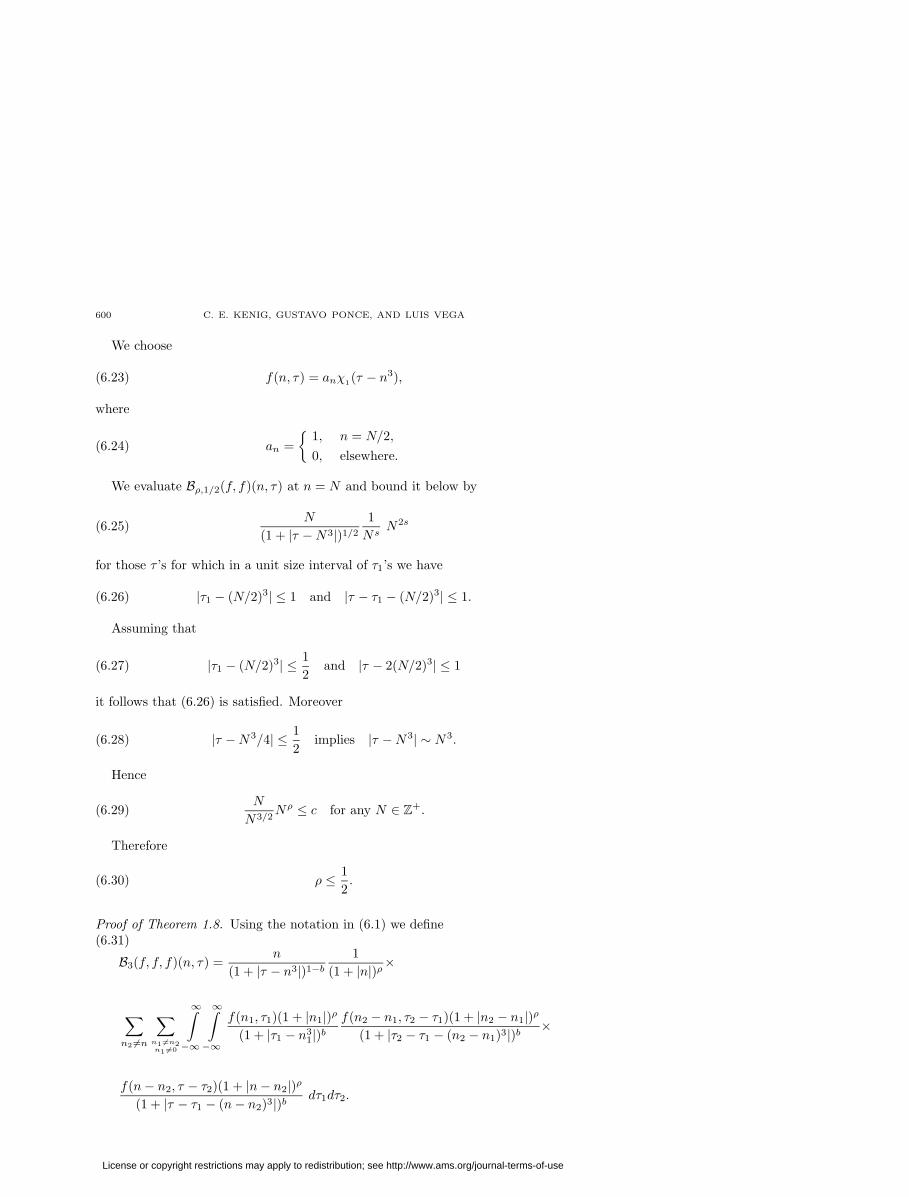
We choose

(6.23) f(n, τ) = anχ1(τ − n3),

where

(6.24) an =

{1, n = N/2,

0, elsewhere.

We evaluate Bρ,1/2(f, f)(n, τ) at n = N and bound it below by

(6.25)N

(1 + |τ −N3|)1/2

1

NsN2s

for those τ ’s for which in a unit size interval of τ1’s we have

(6.26) |τ1 − (N/2)3| ≤ 1 and |τ − τ1 − (N/2)3| ≤ 1.

Assuming that

(6.27) |τ1 − (N/2)3| ≤ 1

2and |τ − 2(N/2)3| ≤ 1

it follows that (6.26) is satisfied. Moreover

(6.28) |τ −N3/4| ≤ 1

2implies |τ −N3| ∼ N3.

Hence

(6.29)N

N3/2Nρ ≤ c for any N ∈ Z+.

Therefore

(6.30) ρ ≤ 1

2.

Proof of Theorem 1.8. Using the notation in (6.1) we define(6.31)

B3(f, f, f)(n, τ) =n

(1 + |τ − n3|)1−b1

(1 + |n|)ρ×

∑n2 6=n

∑n1 6=n2n1 6=0

∞∫−∞

∞∫−∞

f(n1, τ1)(1 + |n1|)ρ(1 + |τ1 − n3

1|)bf(n2 − n1, τ2 − τ1)(1 + |n2 − n1|)ρ

(1 + |τ2 − τ1 − (n2 − n1)3|)b ×

f(n− n2, τ − τ2)(1 + |n− n2|)ρ(1 + |τ − τ1 − (n− n2)3|)b dτ1dτ2.



Thus to obtain (1.19) it suffices to show that

(6.32) ‖B3(f, g, h)‖L2τ`

2n≤ c ‖f‖L2

τ`2n‖g‖L2

τ`2n‖h‖L2

τ`2n

fails for any ρ = −s > 1/2.An argument similar to that used in the proof of Lemma 1 allows us to restrict

ourselves to the case

(6.33) b =1

2.

We now choose

(6.34) f = anχ1/4(τ − n3), g = bnχ1/4

(τ − n3), h = dnχ1/4(τ − n3),

where

(6.35) an =

{1, n = N,

0, elsewhere,bn =

{1, n = −N + 1,

0, elsewhere,dn =

{1, n = N − 1,

0, elsewhere.

Performing the addition and integration in (6.31) in the n1, τ1 variables respec-tively we find

(6.36)

∑n1

an1bn2−n1N2ρ

∫χ

1/4(τ1 − n3

1)χ1/4

(τ2 − τ1 − (n2 − n1)3)dτ1

∼= c∑n1

an1bn2−n1N2ρχ

1/2(τ2 − n3

2 + 3n2n1(n2 − n1))

∼= c αn2N2ρχ

1/2(τ2 − 1− 3N(N − 1)),

where

(6.37) αn2 =

{1, n2 = 1,

0, elsewhere.

Now performing the operations in the n2, τ2 variables we get

(6.38)N3ρ

∑n2

dn−n2αn2

∫χ

1/2(τ2 − 1− 3N(N − 1))χ

1/4(τ − τ2 − (N − 1)3)dτ2

= c N3ρχ(τ −N3).

By inserting this computation in (6.32) it follows that

(6.39) NN3ρ

Nρ≤ c for any N ∈ Z+.

Hence

(6.40) 2ρ+ 1 ≤ 0, i.e. s = −ρ ≥ 1

2.



References

1. B. Birnir, C. E. Kenig, G. Ponce, N. Svanstedt and L. Vega, On the ill-posedness of theIVP for the generalized Korteweg-de Vries and nonlinear Schrodinger equations, to appearJ. London Math. Soc..

2. J. L. Bona and R. Scott, Solutions of the Korteweg-de Vries equation in fractional orderSobolev spaces, Duke Math. J 43 (1976), 87–99. MR 52:14694

3. J. L. Bona and R. Smith, The initial value problem for the Korteweg-de Vries equation, Roy.Soc. London Ser A 278 (1975), 555–601. MR 52:6219

4. J. Bourgain, Fourier restriction phenomena for certain lattice subsets and applications tononlinear evolution equations, Geometric and Functional Anal. 3 (1993), 107-156, 209-262.

MR 95d:35160a,b

5. A. Cohen, Solutions of the Korteweg-de Vries equation from irregular data, Duke Math. J.45 (1978), 149–181. MR 57:10283

6. A. Cohen and T. Kappeler, Solution to the Korteweg-de Vries equation with initial profile inL1

1(R) ∩ L1N (R+), SIAM J. Math. Anal. 18 (1987), 991–1025. MR 88j:35138

7. C. Fefferman, Inequalities for strongly singular convolution operators, Acta Math. 124 (1970),9–36. MR 41:2468

8. , A note on spherical summation multipliers, Israel J. Math. 15 (1973), 44–52. MR47:9160

9. C. S. Gardner, J. M. Greene, M. D. Kruskal and R. M. Miura, A method for solving theKorteweg-de Vries equation, Phys. Rev. Letters 19 (1967), 1095–1097.

10. , The Korteweg-de Vries equation and generalizations. VI. Method for exact solutions,Comm. Pure Appl. Math. 27 (1974), 97–133. MR 49:898

11. T. Kato, Quasilinear equations of evolutions, with applications to partial differential equation,Lecture Notes in Math. 448, Springer (1975), 27–50. MR 53:11252

12. , On the Korteweg-de Vries equation, Manuscripta Math 29 (1979), 89–99. MR80d:35128

13. , On the Cauchy problem for the (generalized) Korteweg-de Vries equation, Advancesin Mathematics Supplementary Studies, Studies in Applied Math. 8 (1983), 93–128. MR86f:35160

14. T. Kappeler, Solutions to the Korteweg-de Vries equation with irregular initial data, Comm.P.D.E. 11 (1986), 927–945. MR 87j:35326

15. C. E. Kenig, G. Ponce and L. Vega, Oscillatory integrals and regularity of dispersive equations,Indiana U. Math. J. 40 (1991), 33-69. MR 92d:35081

16. , Well-posedness of the initial value problem for the Korteweg-de Vries, J. Amer. Math.

Soc 4 (1991), 323–347. MR 92c:35106

17. , Well-posedness and scattering results for the generalized Korteweg-de Vries equationvia the contraction principle, Comm. Pure Appl. Math. 46 (1993), 527-620. MR 94h:35229

18. , The Cauchy problem for the Korteweg-de Vries equation in Sobolev spaces of negativeindices, Duke Math. J. 71 (1993), 1-21. MR 94g:35196

19. S. Klainerman and M. Machedon, Space-time estimates for null forms and the local existencetheorem, Comm. Pure Appl. Math. 46 (1993), 1221–1268. MR 94h:35137

20. , Smoothing estimates for null forms and applications, to appear Duke Math. J.

21. D. J. Korteweg and G. de Vries, On the change of form of long waves advancing in a rectan-gular canal, and on a new type of long stationary waves, Philos. Mag. 5 39 (1895), 422–443.

22. S. N. Kruzhkov and A. V. Faminskii, Generalized solutions of the Cauchy problem for theKorteweg-de Vries equation, Math. U.S.S.R. Sbornik 48 (1984), 93–138. MR 85c:35079

23. H. Lindblad, A sharp counter example to local existence of low regularity solutions to non-linear wave equations, Duke Math. J. 72 (1993), 503-539. MR 94h:35165

24. H. Lindblad and C. D. Sogge, On existence and scattering with minimal regularity for semi-linear wave equations, preprint.

25. R. M. Miura, Korteweg-de Vries equation and generalizations. I. A remarkable explicit non-linear transformation, J. Math. Phys. 9 (1968), 1202-1209. MR 40:6042a

26. H. Pecher, Nonlinear small data scattering for the wave and Klein-Gordon equation, Math.Z. 185 (1984), 261–270. MR 85h:35165

27. G. Ponce and T. C. Sideris, Local regularity of nonlinear wave equations in three space di-mensions, Comm. P.D.E. 18 (1993), 169-177. MR 95a:35092



28. R. L. Sachs, Classical solutions of the Korteweg-de Vries equation for non-smooth initial datavia inverse scattering, Comm. P.D.E. 10 (1985), 29–89. MR 86h:35126

29. J.-C. Saut, Sur quelques generalisations de l’ equations de Korteweg-de Vries, J. Math. PuresAppl. 58 (1979), 21–61. MR 82m:35133

30. J.-C. Saut and R. Temam, Remarks on the Korteweg-de Vries equation, Israel J. Math. 24(1976), 78–87. MR 56:12676

31. A. Sjoberg, On the Korteweg-de Vries equation: existence and uniqueness, J. Math. Anal.Appl. 29 (1970), 569–579. MR 53:13885

32. R. S. Strichartz, Restriction of Fourier transforms to quadratic surface and decay of solutionsof wave equations, Duke Math. J. 44 (1977), 705-714. MR 58:23577

33. S. Tanaka, Korteweg-de Vries equation: construction of solutions in terms of scattering data,Osaka J. Math. 11 (1974), 49–59. MR 50:5231

34. R. Temam, Sur un probleme non lineaire, J. Math. Pures Appl. 48 (1969), 159–172. MR41:5799

35. Y. Tsutsumi, The Cauchy problem for the Korteweg-de Vries equation with measure as initialdata, SIAM J. Math. Anal. 20 (1989), 582–588. MR 90g:35153

36. A. Zygmund, On Fourier coefficients and transforms of functions of two variables, StudiaMath. 50 (1974), 189-201. MR 52:8788

Department of Mathematics, University of Chicago, Chicago, Illinois 60637

E-mail address: [email protected]

Department of Mathematics, University of California, Santa Barbara, California

93106


Departamento de Matematicas, Universidad del Pais Vasco, Apartado 644, 48080 Bil-

bao, Spain



A BILINEAR ESTIMATE WITH APPLICATIONS TO THE KdV EQUATION

Documents

Transcript of A BILINEAR ESTIMATE WITH APPLICATIONS TO THE KdV EQUATION