arX

iv:1

211.

6958

v1 [

nlin

.SI]

29

Nov

201

2

Integrability of reductions of the discrete KdV and potential KdV

equations

A.N.W. Hone, P.H. van der Kamp, G.R.W. Quispel and D.T. Tran

November 30, 2012

Abstract

We study the integrability of mappings obtained as reductions of the discrete Korteweg-de Vries(KdV) equation and of two copies of the discrete potential Korteweg-de Vries equation (pKdV). Weshow that the mappings corresponding to the discrete KdV equation, which can be derived from thelatter, are completely integrable in the Liouville-Arnold sense. The mappings associated with twocopies of the pKdV equation are also shown to be integrable.

1 Introduction

The problem of integrating differential equations goes back to the origins of calculus and its applicationto problems in classical mechanics. In the nineteenth century, the notion of complete integrability wasprovided with a solid theoretical foundation by Liouville, whose theorem gave sufficient conditions for aHamiltonian system to be integrated by quadratures; yet only a few examples of integrable mechanicalsystems (mostly with a small number of degrees of freedom) were known at the time. Poincare’ssubsequent results on the non-integrability of the three-body problem seemed to indicate that thequest for other integrable systems was likely to be fruitless. Nevertheless, examples of integrablesystems (and action-angle variables in particular) played an important role in the early development ofquantum theory.

The theory of integrable systems only began to expand rapidly in the latter part of the twentiethcentury, with the discovery of the remarkable properties of the Korteweg-de Vries (KdV) equation,together with a host of other nonlinear partial differential equations that were found to be amenable tothe inverse scattering technique. As well as having exact pulse-like solutions (solitons) which undergoelastic collisions, such equations could be interpreted as infinite-dimensional Hamiltonian systems, withan infinite number of conserved quantities. Moreover, it was shown that these equations admittedparticular reductions (e.g. to stationary solutions, or to travelling waves) which could be interpreted asintegrable mechanical systems with finitely many degrees of freedom. The papers in the collection [37]provide a concise and self-contained survey of the theory of integrable ordinary and partial differentialequations; for a more recent set of review articles, see [21].

In the last two decades or so, there has been a more gradual development of discrete integrablesystems, in the form of both finite-dimensional maps [24, 5], discrete Painleve equations [26], andpartial difference equations defined on lattices or quad-graphs [22, 1]. Discrete integrable systems can beobtained directly by seeking discrete analogues of particular continuous soliton equations or Hamiltonianflows [30], but they also appear independently in solvable statistical mechanical or quantum models(see [18], for example). An important theoretical result for ordinary difference equations or maps isthe fact that the Liouville-Arnold definition of integrability for Hamiltonian systems can be extendednaturally to symplectic maps [19, 4, 34], so that an appropriate modification of Liouville’s theorem

1

holds. For lattice equations with two or three independent variables there is much less theory available(especially from the Hamiltonian point of view), and the full details of the known integrable examplesare still being explored, but one way to gain understanding is through the analysis of particular familiesof reductions.

By imposing a periodicity condition, integrable lattice equations can be reduced to ordinary differ-ence equations (or mappings) [5, 25, 15, 16]. It is believed that the reduced maps obtained from anintegrable lattice equation are completely integrable in the Liouville-Arnold sense. To prove that a mapis integrable one needs to find a Poisson structure together with a sufficient number of functionallyindependent first integrals, and then show that these integrals commute with respect to the Poissonbracket. One complication that immediately arises is that the reduced maps naturally come in familiesof increasing dimension, and the number of first integrals grows with the dimension. Recently, someprogress has been made with particular families of maps. For maps obtained as reductions of the equa-tions in the Adler-Bobenko-Suris (ABS) classification [1], and for reductions of the sine-Gordon andmodified Korteweg-de Vries (mKdV) equations, first integrals were given in closed form by using thestaircase method and the noncommutative Vieta expansion [31, 17]. In particular, the complete inte-grability of mappings obtained as reductions of the discrete sine-Gordon, mKdV and pKdV equationswas studied in detail in [32, 33].

Given a map, the question arises as to whether it has a Poisson structure, and if so, how can onefind it? In general, we do not know the answer. However, for some classes of maps one can assume thatin coordinates xj the Poisson structure is in canonical or log-canonical form, i.e. the Poisson bracketshave the form xi, xj = Ωij or xi, xj = Ωij xixj respectively, where Ω is a constant skew-symmetricmatrix. This approach is valid for mappings obtained in the context of cluster algebras [12, 9, 10],and also applies to reductions of the lattice potential KdV (pKdV), sine-Gordon and mKdV equations[33]. Another approach requires the existence of a Lagrangian for the reduced map: by using a discreteanalogue of the Ostrogradsky transformation, as introduced in [4], one can rewrite the map in canonicalcoordinates; from there one can derive a Poisson structure in the original variables.

Here we start by considering a well known integrable lattice equation, namely the discrete potentialKorteweg–de Vries equation, also referred to as H1 in the ABS list [1], which is given by

(uℓ,m − uℓ+1,m+1)(uℓ+1,m − uℓ,m+1) = 1, (1)

where (ℓ,m) ∈ Z2. Early results on this equation appear in [36], [5] and [22]. As shown in [36] and [22],

the equation (1) leads to the continuous potential KdV equation, that is

∂u

∂t=∂3u

∂x3+ 3

(∂u

∂x

)2

, (2)

by performing a suitable continuum limit. Using the so-called three-leg form, as in [1], a Lagrangiancan be obtained for the discrete pKdV equation (1). However, the associated Euler-Lagrange equationturns out to consist of two copies of the lattice pKdV equation, that is

uℓ+1,m − uℓ,m+1 + uℓ−1,m − uℓ,m−1 −1

uℓ,m − uℓ+1,m+1+

1

uℓ−1,m−1 − uℓ,m= 0. (3)

The latter equation is somewhat more general than (1): every solution of (1) is a solution of (3), but theconverse statement does not hold. In this paper we shall be concerned with the more general equation(3), rather than (1).

Next, we introduce a new variable on the lattice,

vℓ,m := uℓ,m − uℓ+1,m+1,

2

and immediately find that, whenever uℓ,m is a solution of (3), vℓ,m satisfies

vℓ+1,m − vℓ,m+1 =1

vℓ,m−

1

vℓ+1,m+1. (4)

The latter equation is known as the lattice KdV equation. It is an integrable lattice equation, in thesense that it can be derived as the compatibility condition for an associated linear system, known as aLax pair; this is discussed in section 4.

In this paper we perform the (d − 1,−1)-reduction on the Lagrangian of the pKdV equation andderive the corresponding reduction of the Euler-Lagrange equation (3). This means that we considerfunctions u = uℓ,m on the lattice which have the following periodicity property under shifts:

uℓ,m = uℓ+d−1,m−1. (5)

Such periodicity implies that u depends on the lattice variables ℓ and m through the combination

n = ℓ+m(d− 1)

only; thus, with a slight abuse of notation, we write u = un. Such a reduction can be understood asthe discrete analogue of the travelling wave reduction of a partial differential equation: for a functionu(x, t) satisfying a suitable partial differential equation such as (2), one considers solutions that areinvariant under x→ x+ cδ, t → t+ δ for all δ; such solutions depend on x, t through the combinationz = x−ct only, corresponding to waves travelling with constant speed c. By analogy with the continuouscase, where one obtains ordinary differential equations (with independent variable z) for the travellingwaves, it is apparent that imposing the condition (5) in the discrete setting leads to ordinary differenceequations (with independent variable n). Here we are concerned with the complete integrability ofthe ordinary difference equation obtained as the (d − 1,−1)-reduction of (3), which is equivalent to abirational map in dimension 2d, and the associated reduction of the lattice KdV equation (4), whichgives a map in dimension d.

The paper is organized as follows. In section 2, we start with a discrete Lagrangian for the latticeequation (3), corresponding to two copies of the lattice pKdV equation (1). We then derive a symplecticstructure for the reduced mappings obtained from the discrete Euler-Lagrange equation, by using adiscrete analogue of the Ostrogradsky transformation. This provides a nondegenerate Poisson bracketfor each of these maps. In section 3 we present a Poisson structure for the mapping obtained as the(d−1,−1)-reduction of the lattice KdV equation (4), for each d, which is induced from the bracket foundin section 2. The Hirota bilinear form of each of these mappings is also given, in terms of tau-functions,whence (via a link with cluster algebras) we derive a second Poisson structure that is compatible withthe first. In section 4 we present closed-form expressions for integrals of the reduced KdV map, fittinginto the framework of the papers [31] and [33], which furnishes a direct proof of Liouville integrability.Another proof, based on the pair of compatible Poisson brackets, is also sketched. The construction offirst integrals is done using the staircase method, the noncommutative Vieta expansion and a suitablesplitting of Lax matrices. In section 5, for each d we present integrals for the mapping obtained asthe (d− 1,−1)-reduction of the discrete Euler-Lagrange equation (3). Some integrals are derived fromthe integrals of the KdV map in the previous section, while additional commuting integrals for thereduction of (3) are found using a function periodic with period d; this is a d-integral, in the sense of[13]. The paper ends with some brief conclusions, followed by a proof that is relegated to an Appendix.

3

2 Nondegenerate Poisson structure from two copies of pKdV

Henceforth, it is convenient to use ˜ and to denote shifts in ℓ and m directions respectively, so thatu = uℓ+1,m, u = uℓ,m+1, etc. It is known that all equations of the form

Q(u, u, u, u, α, β) = 0 (6)

in the ABS list [1] are equivalent (up to some transformations) to the existence of an equation ofso-called three-leg type, that is

P (u, u, u, u;α, β) ≡ φ(u, u, α)− φ(u, u, β) − ψ(u, u, α, β) = 0, (7)

for suitable functions φ,ψ, where α and β are parameters; the latter leads to the derivation of a La-grangian for each of the equations (6). In particular, for the pKdV equation (1), which is a (parameter-

free) equation of the form (6), we have φ(u, u) = u+ u and ψ(u, u) = 1/(u− u), and using the three-legform (7) leads to the Lagrangian

L =1

2(u+ u)2 −

1

2(u+ u)2 − log |u− u|. (8)

The corresponding discrete Euler-Lagrange equation is the equation (3), which can be rewritten as

J = J, with J = u− u−

1

(u− u). (9)

The latter equation is more general than (1), which arises in the special case that J is identically zero.Now we set n = ℓ + m(d − 1), with u satisfying (5), and apply the (d − 1,−1)-reduction to the

Lagrangian L in (8), to find

L (un, un+1, . . . , un+d) =1

2(un + un+1)

2 −1

2(un + un+d−1)

2 − log |un − un+d|. (10)

The discrete action functional is S :=∑

n∈Z L (un, un+1, . . . , un+d). It yields the discrete Euler-Lagrangeequation

δS

δun=

d∑

r=0

∂L (un−r, un+1−r, . . . , un+d−r)

∂un=

d∑

r=0

E−rLr = 0, (11)

where E denotes the shift operator and Lr =∂L(un,un+1,...,un+d)

∂un+r. Thus we obtain the ordinary difference

equation

un+1 − un+d−1 + un−1 − un−d+1 −1

un − un+d+

1

un−d − un= 0, (12)

which is precisely the (d− 1,−1)-reduction of (3). The solutions of this equation are equivalent to theiterates of the 2d-dimensional map

(un−d, un−d+1, . . . , un+d−1) 7→ (un−d+1, un−d+2, . . . , un+d), (13)

where un+d is found from equation (12).Given a Lagrangian of first order for a classical mechanical system, the Legendre transformation

produces canonical symplectic coordinates on the phase space; the Ostrogradsky transformation is theanalogue of this for Lagrangians of higher order [2]. In order to derive a nondegenerate Poisson bracket

4

for the 2d-dimensional map, we use a discrete analogue of the Ostrogradsky transformation, as givenin [4], which is a change of variables to canonical coordinates,

(un−d, . . . , un, . . . , un+d−1) → (q1, . . . , qd, p1, . . . , pd),

where

qi = un+i−1, pi = E−1d−i∑

r=0

E−rLr+i.

Thus, from (10), we obtain

qi = un+i−1, i = 1, . . . , d,

p1 = −un+1 + un+d−1 +1

un − un+d= un−1 − un+1−d +

1

un−d − un,

pi = −un+i−d − un+i−1 +1

un−d+i−1 − un+i−1, i = 2, . . . , d− 1,

pd =1

un−1 − un+d−1.

In terms of the canonical coordinates qj , pj the map (12) is rewritten as

qi 7→ qi+1, i = 1, . . . , d− 1, qd 7→ q1 − (p1 + q2 − qd)−1,

p1 7→ p2 + q2 + q1, pi 7→ pi+1, i = 2, . . . , d− 2,pd−1 7→ pd − q1 − qd, pd 7→ p1 + q2 − qd.

By the general results in [4], this map is symplectic with respect to the canonical symplectic form∑dj=1 dpj ∧ dqj. Equivalently, it preserves the canonical Poisson brackets

pi, pj = qi, qj = 0, pi, qj = δij .

In order to find the Poisson brackets for the coordinates un, we write them in terms of (qj, pj). Forall 0 ≤ i ≤ d− 1, we have un+i = qi+1 and

un−1 = qd + 1/pd = [qd; pd],

un−2 = qd−1 +1

pd−1 + qd+1 + un−1= [qd−1; pd−1 + qd−1 + qd, pd],

un−i−1 = [qd−i; pd−i + qd−i + un−i]

= [qd−i; pd−i + qd−i + qd−i+1, pd−i+1 + qd−i+1 + qd−i+2, . . . , pd−1 + qd−1 + qd, pd], 1 ≤ i ≤ d− 2,

un−d = [q1; p1 + un+1−d − un−1]

= [q1; p1 − qd + q2 −1

pd, p2 + q2 + q3, . . . , pd−1 + qd−1 + qd, pd],

where [ ; ] denotes a continued fraction. This yields the following result, proved in the Appendix.

Theorem 1. The 2d-dimensional map given by (13) with (12) is a Poisson map with respect to thenondegenerate bracket

un−d, un−j−1 = 0, 0 ≤ j ≤ d− 1; (14)

un−d, un+j = (−1)j+1(un−d − un)2 . . . (un−d+j − un+j)

2, 0 ≤ j < d− 1; (15)

un−d, un+d−1 = (−1)d(un−d − un)2 . . . (un−1 − un+d−1)

2 − (un−d − un)2(un−1 − un+d−1)

2. (16)

5

3 Poisson structures and tau-functions for KdV maps

As mentioned above, the discrete KdV equation can be derived from two copies of the pKdV equation.This suggests that we can find a Poisson structure for the (d − 1,−1)-reduction of the discrete KdVequation using the symplectic structure given in the previous section. It turns out that, in additionto the bracket induced from two copies of pKdV, each of the KdV maps has a second, independentPoisson bracket, which is obtained from a Hirota bilinear form in terms of tau-functions. The secondbracket is constructed by making use of a connection with Somos recurrences and cluster algebras.

3.1 First Poisson structure from pKdV

Upon introducing the quantitiesvn := un−d − un,

we see that, whenever un is a solution of equation (12), vn satisfies a difference equation of order d,namely

vn+d−1 − vn+1 −1

vn+d+

1

vn= 0. (17)

Alternatively, by starting from a solution of (3) with the periodicity property (5), we see that this yieldsa solution v = vℓ,m of (4) with the same periodicity, and so (writing this as vn, with the same abuse ofnotation as before) it is clear that equation (17) is just the (d − 1,−1)-reduction of the discrete KdVequation. Equivalently, the ordinary difference equation (17) corresponds to the d-dimensional map

ϕ : (v0, v1, . . . , vd−1) 7→

(v1, v2, . . . , vd−1,

v01 + vd−1v0 − v1v0

). (18)

The case d = 2 is trivial, so henceforth we consider d ≥ 3.In the above, the suffix n has been dropped, taking a fixed d-tuple (v0, v1, . . . , vd−1) in d-dimensional

space. However, because the map (18) is obtained from a recurrence of order d, all of the formulae areinvariant under simultaneous shifts of all indices by an arbitrary amount n, i.e. vj → vn+j for eachj. For a fixed n, say n = 0, the formulae in Theorem 1 define a Poisson bracket in dimension 2d,which can be used to calculate the brackets between the quantities vj = uj−d − uj for j = 0, . . . , d− 1.Remarkably, these brackets can be rewitten in terms of vj alone; in other words, these quantities forma Poisson subalgebra of dimension d. Hence this provides the first of two ways to endow (18) with aPoisson structure.

Theorem 2. The d-dimensional map (18) is a Poisson map with respect to the bracket , 1 definedby

vi, vj1 =

(−1)j−i

∏jr=i v

2r , 0 < j − i < d− 1,(

1 + (−1)d−1∏d−2

r=1 v2r

)v20v

2d−1, j − i = d− 1.

(19)

This bracket is degenerate, with one Casimir when d is odd, and two independent Casimirs when d iseven.

The above result follows immediately from Theorem 1, apart from the statement about the Casimirs,which will be explained shortly. Here we first give a couple of examples for illustration.

Example 3. When d = 3 the map ϕ given by (18) preserves the Poisson bracket

v0, v11 = −v20v21 , v1, v21 = −v21v

22 , v0, v21 = (1 + v21)v

20v

22 .

6

This bracket has rank two, with a Casimir C that is also a first integral for the map:

C = v1−1

v0−

1

v1−

1

v2, and ϕ∗C = C. ♦

Example 4. When d = 4 the map (18) preserves the Poisson bracket specified by

v0, v11 = −v20v21 , v0, v21 = v20v

21v

22 , v0, v31 = (1− v21v

22)v

20v

23,

where all other brackets vi, vj1 for 0 ≤ i, j ≤ d − 1 are determined from skew-symmetry and thePoisson property of ϕ. This is a bracket of rank two, having two independent Casimirs given by

C1 = v1−1

v0−

1

v2, C2 = v2−

1

v1−

1

v3, with ϕ∗C1 = C2, ϕ∗C2 = C1. ♦

Remark 5. The Casimirs Cj in the preceding example are 2-integrals [13], meaning that they arepreserved by two iterations of the map, i.e. (ϕ∗)2Cj = Cj for j = 1, 2. The symmetric functions

K = C1 + C2, K′ = C1C2 (20)

provide two independent first integrals.

In order to make the properties of the Poisson bracket , 1 more transparent, we introduce somenew coordinates, the motivation for which should become clear from the Lax pairs in section 4.

Lemma 6. For all d ≥ 4, with respect to the coordinates

g0 = −1/v0, gj = vj−1 − 1/vj , j = 1, . . . , d− 1, (21)

the first Poisson bracket for the KdV map (18) is specified by the following relations for ν = 1 and0 ≤ i < j ≤ d− 1:

gi, gj1 =

−1 if j − i = 1,1 if j − i = d− 1,ν/g20 if i = 1, j = d− 1,0 otherwise.

(22)

When d is odd this bracket has the Casimir

C = g0 + g1 + . . .+ gd−1 +ν

g0, (23)

while for even d there are the two Casimirs

C1 = g0 + g2 + . . .+ gd−2, C2 = g1 + g3 + . . .+ gd−1 +ν

g0. (24)

Remark 7. When ν = 0 the Poisson bracket (22) is just the first Poisson bracket for the dressingchain, as given by equation (13) in [35].

In terms of the coordinates gj, the map (18) is rewritten as

ϕ : (g0, g1, . . . , gd−1) 7→

(g1 +

1

g0, g2, . . . , gd−1,

g20g11 + g0g1

). (25)

Note that for the special case d = 3, as in Example 3, part of the formula for the bracket (22) requiresa slight modification, namely

g1, g21 = −1 + 1/g20 .

7

3.2 Second Poisson structure from cluster algebras for tau-functions

The discrete KdV equation (4) was derived by Hirota in terms of tau-functions, via the Backlundtransformation for the differential-difference KdV equation [14]. In Hirota’s approach, the solution of

the discrete KdV equation is given in terms of a tau-function as v = τ τ /(τ τ ), and at the level of the(d− 1,−1)-reduction this becomes

vn =τn+1 τn+d−1

τn τn+d. (26)

By direct substitution, it then follows that vn is a solution of (17) provided that τn satisfies the trilinear(degree three) recurrence relation

τn+2d τn+d−1 τn+1 = τn+2d−1 τn+d+1 τn − τn+2d−1 τn+d−1 τn+2 + τn+2d−2 τn+d+1 τn+1. (27)

However, this relation can be further simplified upon dividing by τn+1τn+d, which gives the relation

αn =τn τn+d+1 − τn+2τn+d−1

τn+1 τn+d=τn+d−1 τn+2d − τn+d+1τn+2d−2

τn+d τn+2d−1= αn+d−1.

This immediately yields relations that are bilinear (degree two) in τn.

Proposition 8. The solutions of the equation (17) are given in terms of a tau-function by (26), whereτn satisfies the bilinear recurrence relation

τn+d+1 τn = αn τn+d τn+1 + τn+d−1 τn+2 (28)

of order d+ 1, with the coefficient αn having period d− 1.

Apart from the presence of the periodic coefficient αn, the bilinear relation (28) has the form of aSomos-(d + 1) recurrence [29]. Such recurrence relations (with constant coefficients) are also referredto as three-term Gale-Robinson recurrences (after [11] and [28] respectively).

Example 9. For d = 3 the equation (28) is a Somos-4 recurrence with coefficients of period 2:

τn+4 τn = αn τn+3 τn+1 + τ2n+2, αn+2 = αn.

Due to the Laurent phenomenon [7], the iterates of this recurrence are Laurent polynomials, i.e. poly-nomials in the initial values data and their reciprocals with integer coefficients; to be precise,

τn ∈ Z[α0, α1, τ±10 , τ±1

1 , τ±12 , τ±1

3 ]

for all n ∈ Z. This means that integer sequences can be generated from a suitable choice of initial dataand coefficients. For instance, with the initial values τ0 = τ1 = τ2 = τ3 = 1 and parameters α0 = 1,α1 = 2, the Somos-4 recurrence yields an integer sequence beginning with

1, 1, 1, 1, 2, 5, 9, 61, 193, 1439, 13892, 121853, 1908467, 47166783, . . . . ♦

From the work of Fordy and Marsh [8], it is known that, at least in the case where the coefficients areconstant, recurrences of Somos type can be generated from sequences of mutations in a cluster algebra.For the purposes of this paper, the main advantage of considering the cluster algebra is that it providesa natural presymplectic structure for the tau-functions. A presymplectic form that is compatible withcluster mutations was presented in [12], and in [10] it was explained how this presymplectic structureis preserved by the recurrences considered in [8].

8

Cluster algebras are a new class of commutative algebras which were introduced in [6]. Rather thanhaving a set of generators and relations that are given from the start, the generators of a cluster algebraare defined recursively by an iterative process known as cluster mutation. For a coefficient-free clusteralgebra, one starts from an initial set of generators (the initial cluster) of fixed size, which here we taketo be d + 1. If the initial cluster is denoted by (τ1, . . . , τd+1), then for each index k one defines themutation in the k direction to be the transformation that exchanges one of the variables to produce anew cluster (τ ′1, . . . , τ

′d+1) given by

τ ′j = τj, j 6= k, τ ′k τk =

d+1∏

j=1

τ[bjk]+j +

d+1∏

j=1

τ[−bjk]+j , (29)

where the exponents in the exchange relation for τ ′k come from an integer matrix B = (bij) known asthe exchange matrix, and we have used the notation [b]+ = max(b, 0).

As well as cluster mutation, there is an associated operation of matrix mutation, which acts on thematrix B; the details of this are omitted here. Fordy and Marsh gave conditions under which skew-symmetric exchange matrices B have a cyclic symmetry (or periodicity) under mutation, and classifiedall such B with period 1 [8]. They also showed how this led to recurrence relations for cluster variables,by taking cyclic sequences of mutations. The requirement of periodicity puts conditions on the elementsof the skew-symmetric matrix B, which (for a suitable labelling of indices) can be written as

bi,d+1 = b1,i+1, i = 1, . . . , d, (30)

andbi+1,j+1 = bi,j + b1,i+1[−b1,j+1]+ − b1,j+1[−b1,i+1]+, 1 ≤ i, j ≤ d. (31)

The corresponding recurrence is defined by iteration of the map

(τ1, . . . , τd, τd+1) 7→ (τ2, . . . , τd+1, τ′1)

associated with the exchange relation (29) for index k = 1, where the exponents are given by the entriesb1,j in the first row of B. Moreover, given a recurrence relation of this type, the conditions (30) and(31) allow the rest of the matrix B to be constructed from the exponents corresponding to the firstrow, and these conditions are also necessary and sufficient for a log-canonical presymplectic form ω, asin (32) below, to be preserved (see Lemma 2.3 in [10]). In general this two-form is closed, but it maybe degenerate.

For the case at hand, the exponents appearing in the two monomials on the right hand side of (28)specify the first row of the matrix B as (0, 1,−1, 0, . . . , 0,−1, 1), and the rest of this matrix is foundby applying (30) and (31). Although the foregoing discussion was put in the context of coefficient-free cluster algebras, the presence of coefficients in front of these two monomials does not affect thebehaviour of the corresponding log-canonical two-form under iteration. Thus we obtain

Lemma 10. For all d ≥ 5, the Somos-(d + 1) recurrence (8) preserves the presymplectic form

ω =∑

i<j

bijτiτj

dτi ∧ dτj, (32)

given in terms of the entries of the associated skew-symmetric exchange matrix B = (bij) of size d+1,

9

where (with an asterisk denoting the omitted entries below the diagonal)

B =

0 1 −1 0 · · · 0 −1 1. . . 2 −1 0 · · · 1 −1

. . .. . .

. . .. . . 0

. . .. . .

. . .. . .

.... . .

. . .. . . 0

. . . 2 −1∗ 0 1

0

.

Remark 11. In each of the special cases d = 3, 4, the exchange matrix does not fit into the generalpattern above. For the details of the case d = 3, when (28) is a Somos-4 relation, see Example 2.11 in[10]; and for d = 4 (Somos-5) see Example 1.1 in [9].

The exchange matrices being considered here are all degenerate: for d odd, B has a two-dimensionalkernel, while for d even, the kernel is three-dimensional. In the odd case, the kernel is associated withthe action of a two-parameter group of scaling symmetries, namely

τn → ρ σn τn, ρ, σ 6= 0, (33)

while in the even case there is the additional symmetry

τn → ξ(−1)n τn, ξ 6= 0; (34)

in the theory of tau-functions such scalings are known as gauge transformations. By Lemma 2.7 in [10](see also section 6 therein), symplectic coordinates are obtained by taking a complete set of invariantsfor these scaling symmetries. With a suitable choice of coordinates, denoted below by yn, the associatedsymplectic maps can be written in the form of recurrences, like so:

• Odd d: The quantities yn = τn+2τn/τ2n+1 are invariant under (33), and satisfy the difference

equationyn+d−1 (yn+d−2 · · · yn+1)

2 yn = αn yn+d−2 · · · yn+1 + 1. (35)

• Even d: The quantities yn = τn+3τn/(τn+2τn+1) are invariant under both (33) and (34), andsatisfy the difference equation

yn+d−2 · · · yn = αn yn+d−3yn+d−5 · · · yn+1 + 1. (36)

Example 12. Both of the cases d = 3 and d = 4 lead to iteration of maps in the plane with coefficientsthat vary periodically, namely

d = 3 : yn+2 y2n+1 yn = αn yn+1 + 1, with αn+2 = αn,

and

d = 4 : yn+2 yn+1 yn = αn yn+1+1, with αn+3 = αn. ♦

Remark 13. Due to the presence of the periodic coefficients, the latter maps are not of standard QRTtype [24], but they reduce to symmetric QRT maps when αn =constant. Maps in the plane of this moregeneral type have recently been studied systematically by Roberts [27].

10

In general, the solutions of (35) or (36) correspond to the iterates of a symplectic map, in dimensiond− 1 or d− 2, respectively. To be more precise, rather than just iterating a single map, each iterationdepends on the coefficient αn which varies with a fixed period (as in Proposition 8), but the samesymplectic structure is preserved at each step. The appropriate symplectic form in the coordinates yncan be obtained from (32), and by a direct calculation the associated nondegenerate bracket is found;this is presented as follows.

Lemma 14. For d odd, each iteration of (35) preserves the nondegenerate Poisson bracket specified by

yi, yj = (−1)j−i+1 yi yj, 0 ≤ i < j ≤ d− 2. (37)

For d even, the map defined by (36) preserves the nondegenerate bracket in dimension d− 2 given by

yi, yi±1 = ± yi yi±1, (38)

with all other brackets yi, yj for 0 ≤ i < j ≤ d− 3 being zero.

The bracket for the variables yi is the key to deriving a second Poisson structure for the KdV mapswhen d is odd.

Theorem 15. In the case that d is odd, the map (18) preserves a second Poisson bracket, which isspecified in terms of the coordinates (21) by

gi, gj2 = (−1)j−i+1 gi gj, 0 ≤ i < j ≤ d− 1. (39)

Proof. Substituting for vn from the formula (26) and making use of the bilinear equation (28) producesthe identities

vj−1 −1

vj=τj(τj+1τj+d−2 − τj−1τj+d)

τj+d−1τj−1τj+1= −

αj−1τ2j

τj−1τj+1,

so that, by the definition of the symplectic coordinates yj,

gj = −αj−1

yj−1, j = 1, . . . , d− 1.

A similar calculation in terms of tau-functions also yields

g0 = −y0 y1 · · · yd−2.

Noting that the coefficients αi play the role of constants with respect to the bracket (37), this immedi-ately implies that the induced brackets between the gi are

gi, gj = αi−1αj−1y−2i−1y

−2j−1yi−1, yj−1 = (−1)j−i+1gigj

for 1 ≤ i < j ≤ d− 1, which agrees with (39). By making use of the preceding formula for g0 in termsof yi, the brackets g0, gj follow in the same way.

Remark 16. The bracket (39) is the same as the quadratic bracket for the dressing chain (for the casewhere all parameters βi are zero in [35]). It has the Casimir

C∗ = g0 g1 · · · gd−1, (40)

which is also given in terms of the coefficients of the bilinear equation (28) by C∗ = −∏d−2

j=0 αj .

11

The case where d is even is slightly more complicated, because we do not have a direct way to derivea second Poisson bracket in terms of the coordinates gi (or equivalently vi). The reason for this difficultyis that, from the tau-function expressions, although the quantities gi remain the same under the actionof the two-parameter symmetry group (33), they are not invariant under the additional scaling (34),but rather they transform differently according to the parity of the index i:

gi −→ ξ±4 gi for even/odd i. (41)

In order to obtain a fully invariant set of variables, we introduce a projection π from dimension d todimension d− 1:

π : fi = gigi+1, i = 0, . . . , d− 2.

By regarding the new coordinates fi as functions of the gj, we get an induced map ϕ′ in dimensiond− 1, which is compatible with ϕ in the sense that ϕ · π = π · ϕ′; this has the form

ϕ′ : (f0, f1, . . . , fd−2) 7→

(f1(1 + f−1

0 ), f2, . . . , fd−2,f0f2 · · · fd−2

(1 + f−10 )f1f3 · · · fd−3

). (42)

In terms of tau-functions, the quantities fi are invariant under the action of the full three-parametergroup of gauge transformations, which means that they can be expressed as functions of the invariantsymplectic coordinates yn, and hence we can derive a Poisson bracket for them.

Theorem 17. In the case that d is even, the map (42) preserves a Poisson bracket, which is specifiedin terms of the coordinates fi by

fi, fi±12 = ± fi fi±1, (43)

with all other brackets fi, fj2 for 0 ≤ i < j ≤ d− 2 being zero.

Proof. Following the proof of Theorem 15, we have

gigi+1 =αi−1αiτiτi+1

τi−1τi+2,

whence, in terms of the symplectic coordinates for (36), we have

fi =αi−1αi

yi−1, i = 1, . . . , d− 2.

A similar calculation yields a slightly different formula for index i = 0:

f0 = α0 y1y3 · · · yd−3,

and then the Poisson brackets (38) between the yj directly imply that the brackets (43) hold betweenthe fi.

Remark 18. The bracket (43) has the Casimir

C∗ = f0 f2 · · · fd−2, (44)

which is also given in terms of the coefficients of the bilinear equation (28) by C∗ =∏d−2

j=0 αj .

It may be unclear why there is the suffix 2 on the bracket in (43), since we have not yet providedanother Poisson bracket for the map (42). However, as will be explained in the next section, when dis even the quantities fi form a Poisson subalgebra for the bracket , 1 of Theorem 2. As will alsobe explained, the brackets , 1 and , 2 are compatible (in the sense that any linear combination ofthem is also a Poisson bracket), which means that a standard bi-Hamiltonian argument can be used toshow Liouville integrability of the maps for either odd or even d.

12

4 First integrals and integrability of the KdV maps

The purpose of this section is to prove the following result.

Theorem 19. For each d ≥ 3, the map (18) is completely integrable in the Liouville sense.

Recall that, for a Poisson map ϕ in dimension d, Liouville integrability means that there should bek Casimirs invariant under the map, so that the (d − k)-dimensional symplectic leaves of the Poissonbracket are preserved by ϕ, plus an additional 1

2(d−k) independent first integrals that are in involutionwith respect to the bracket. For the particular map in question, there is always the Poisson bracket , 1, and from Lemma 6 this has either one or two Casimirs, with symplectic leaves of dimension d−1or d− 2, for odd/even d respectively; hence an additional ⌊12(d− 1)⌋ first integrals are required in thiscase.

For the lowest values d = 3, 4, it is straightforward to verify complete integrability, since in thosecases only one extra first integral is required, apart from the Casimirs of , 1. When d = 3, as inExample 3, the Casimir C is preserved by ϕ; the quantity C∗ in (40), which is the Casimir of the secondbracket, is also a first integral. Similarly, for d = 4, the two Casimirs in Example 4 provide the two firstintegrals (20), which are themselves Casimirs; the quantity C∗ = f0f2 = g0g1g2g3, as in (44), providesthe extra first integral.

Example 20. For d = 3, each of the first integrals C, C∗ of the map (18) define surfaces in threedimensions, given by

XY 2Z − CXY Z −XY − Y Z − ZX = 0, XY 2Z + C∗XY Z −XY − Y Z + 1 = 0,

respectively, in terms of coordinates (X,Y,Z) ≡ (vn, vn+1, vn+2). These two surfaces intersect in acurve of genus one, found explicitly by eliminating the variable Z above; this yields the biquadratic

(C + C∗)X2Y 2 + (X + Y )(XY − 1)− CXY = 0. (45)

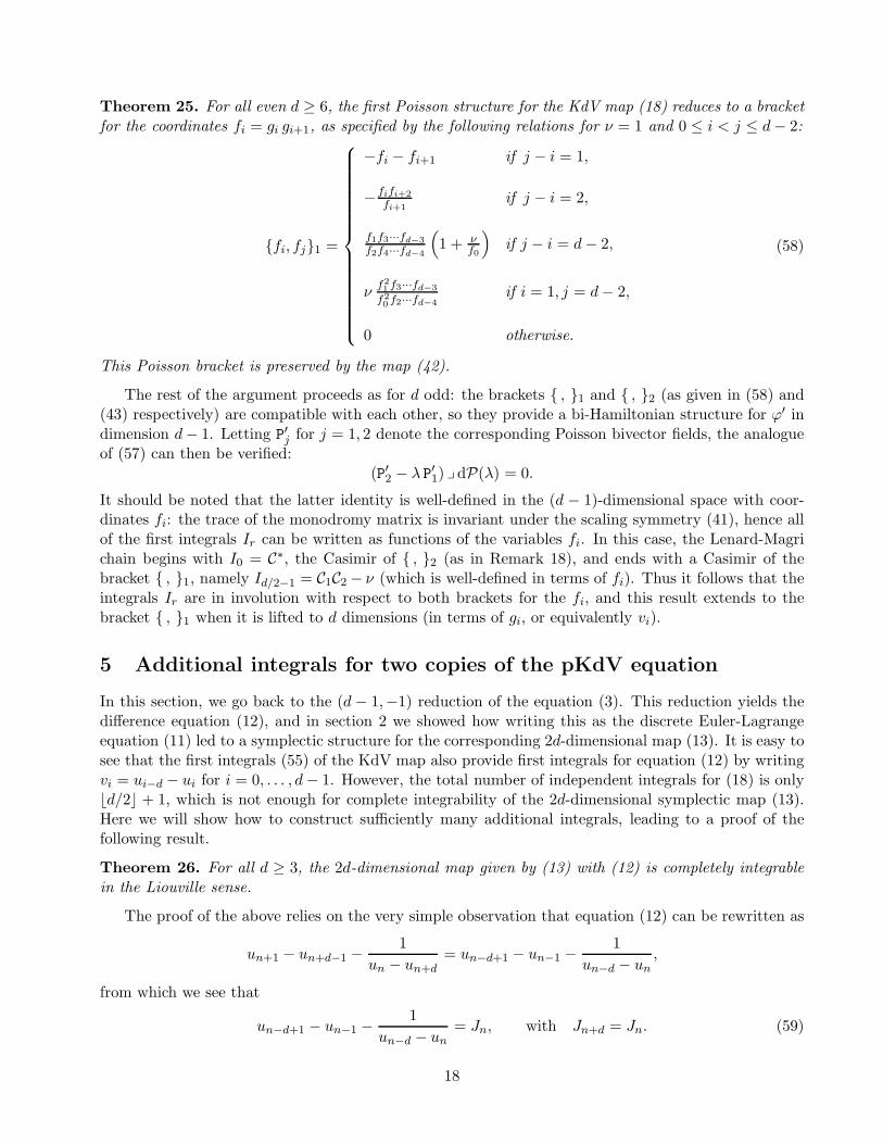
The embedding of such a curve in three dimensions can be seen from the orbit plotted in Figure 1. ♦

For higher values of d, it is not so obvious how to proceed, but the correct number of additionalfirst integrals can be obtained by constructing a Lax pair for the map, as we now describe.

4.1 Lax pairs and monodromy

The discrete KdV equation (4) is known to be integrable in the sense that it arises as the compatibilitycondition for a pair of linear equations. In [23], a scalar Lax pair is given as follows:

φ = vφ+ λφ, φ = φ+

1

vφ.

Upon introducing the vector Φ :=

(φφ

), the latter pair of scalar equations leads to a Lax pair in

matrix form, namely

Φ = LΦ, Φ = MΦ, with L =

(v − 1

v λ1 0

), M =

(v λ1 1

v

). (46)

Equation (4) is equivalent to the compatibility condition for the linear system (46), that is

LM = ML. (47)

13

0.4

0.6

0.8

1

0.4

0.6

0.8

1

0.4

0.6

0.8

1

Figure 1: The orbit of the map (18) for d = 3 with initial data (v0, v1, v2) = (1, 12, 25).

Note that the matrix L is associated with shifts in the ℓ (horizontal) direction, and M with shifts inthe m (vertical) direction.

First integrals of each KdV map (18) can be found by using the staircase method [5, 25, 15, 16]. Forthe (d− 1,−1)-reduction, a staircase on the Z2 lattice is built from paths consisting of d− 1 horizontalsteps and one vertical step. Taking an ordered product of Lax matrices along the staircase yields themonodromy matrix

Ln = M−1n Ln+d−2 · · ·Ln, (48)

corresponding to d− 1 steps to the right (ℓ → ℓ+ 1) and one step down (m → m− 1), where L → Ln

and M → Mn under the reduction. As a consequence of (47), the identity Ln+d−1Mn = Mn+1Ln

holds, which implies that Ln satisfies the discrete Lax equation

Ln Ln = Ln Ln+1. (49)

The latter holds if and only if vn satisfies the difference equation (17). Since (49) means that thespectrum of Ln is invariant under the shift n→ n+1, first integrals for the KdV map can be constructedfrom the trace of the monodromy matrix (or powers thereof), which can be expanded in the spectralparameter λ.

For convenience, we conjugate Ln in (48) by Mn and multiply by an overall factor of λ− 1, which(upon setting n = 0) gives a modified monodromy matrix

L† = L†d−1 · · ·L

†1L

†0, (50)

where

L†i = Li−1 =

(gi λ1 0

), i = 1, . . . , d− 1, but L†

0 =

(g0 λ1 ν

g0

)with ν = 1.

14

Thus we see the origin of the coordinates gi introduced in Lemma 6: they are the (1, 1) entries in theLax matrices that make up the monodromy matrix. We have already mentioned a connection withthe dressing chain at the level of the Poisson brackets, but it can be seen more directly here: up totaking an inverse and inserting a spectral parameter, when ν = 0 the expression (50) reduces to themonodromy matrix for the dressing chain found in [10]. The parameter ν can be regarded as introducinginhomogeneity into the chain at i = 0 (and for ν 6= 0 it is always possible to rescale so that ν = 1).

With the introduction of another spectral parameter µ, we consider the characteristic polynomialof L†, which defines the spectral curve

χ(λ, µ) := det(L† − µ 1) = µ2 − P(λ)µ + (ν − λ)(−λ)d−1 = 0, (51)

with P(λ) = trL†. This curve in the (λ, µ) plane is invariant under the KdV map (18), and the traceof L† provides the polynomial P whose non-trivial coefficients are first integrals of the map.

Example 21. When d = 3 the spectral curve is

µ2 − (C∗ + Cλ)µ+ (ν − λ)λ2 = 0,

which has genus one, and (for ν = 1) is isomorphic to the biquadratic curve (45) corresponding to theintersection of the level sets of C and C∗. ♦

Example 22. When d = 4 the spectral curve also has genus one, being given by

µ2 − (I0 + I1 λ+ 2λ2)µ− (ν − λ)λ3 = 0,

with coefficients expressed in terms of gi by

I0 = C∗ = g0g1g2g3, I1 = K′−ν = g0g1+g1g2+g2g3+g3g0+νg2g0. ♦

In the next subsection, we will show how, for each d, expanding the trace of the monodromy matrixin powers of λ gives the polynomial P of degree ⌊d/2⌋. This implies that the hyperelliptic curveχ(λ, µ) = 0 as in (51) has genus ⌊12 (d− 1)⌋. Thus we expect that the (real, compact) Liouville tori forthe KdV map should be identified with (a real component of) the Jacobian variety of this curve, sincetheir dimensions coincide, and the map should correspond to a translation on the Jacobian.

4.2 Direct proof from the Vieta expansion

In order to calculate the trace of the monodromy matrix explicitly, we split the Lax matrices as

L†i = λ

(0 10 0

)+

(gi 01 0

)= λX+Yi, i = 1, . . . d− 1, (52)

and similarly for L†0. This splitting fits into the framework of [31], with the coefficient of λ being the

same nilpotent matrix X in each case, and allows the application of the so-called Vieta expansion.Recall that, in the noncommutative setting, the Vieta expansion is given by the formula

x

b∏

i=a

(λXi +Yi) := (λXb +Yb) . . . (λXa +Ya) =

b−a+1∑

r=0

λrZa,br ,

whereZa,br =

∑

a≤i1<i2<···<ir≤b

YbYb−1 · · ·Yir+1XirYir−1 · · ·Yi1+1Xi1Yi1−1 · · ·Ya. (53)

In the case at hand, we have Xi = X for all i, and by writing the monodromy matrix in the form (53),we can use Lemma 8 in [31], so that the trace is expanded as

P(λ) = trL† =

⌊d/2⌋∑

r=0

Ir λr, (54)

where the first integrals of the KdV map are given by the closed-form expression

Ir = Ψ1,d−3r−1 + g0Ψ

1,d−4r−1 +

(gd−1 +

ν

g0

)Ψ2,d−3

r−1 +Ψ2,d−4r−2 + g0gd−1Ψ

1,d−3r , (55)

with

Ψa,br =

b+1∏

i=a

gi

∑

a≤i1<i1+1<i2...<ir≤b

r∏

j=1

1

gijgij+1

. (56)

The explicit form of these integrals mean that it is possible to give a direct verification that they arein involution, which is almost identical to the proof of Theorem 13 in [33].

Proposition 23. The first integrals (55) of the KdV map Poisson commute with respect to the bracket , 1 in (19).

Proof. Writing the Poisson structure in terms of the coordinates gi as in Lemma 6, we see that (up toan overall factor of −1) the brackets gi, gj1 in (22) for 1 ≤ i, j ≤ d − 2 are identical to the bracketsbetween the coordinates ci given by equation (46) in [33]. The polynomial functions given by (56) are

the same as in the latter reference, and the particular functions Ψa,br that appear in the formula (55)

only depend on gi for 1 ≤ i ≤ d − 2. This implies that the brackets between these functions are thesame as those given in Lemma 11 and Corollary 12 in [33], whence it is straightforward to verify thatIr, Is1 = 0 for 0 ≤ r, s ≤ ⌊d/2⌋.

In order to complete the proof of Theorem 19, it only remains to check that there are sufficientlymany independent integrals.

For odd d, the leading (ν = 0) part of the first integral Ir is a cyclically symmetric, homogeneousfunction of degree d− 2r in the gi, being identical to the independent integrals of the dressing chain in[35] (for parameters βi = 0), with terms of each odd degree appearing for r = 0, . . . , d−1

2 . Hence thesefunctions are also independent in the case ν 6= 0, corresponding to the addition of a rational term withg0 in the denominator, which is linear in ν and of degree d − 2r − 2 in the gi. This means that thereare degP = (d − 1)/2 + 1 independent integrals, of which the last one is I(d−1)/2 = C, the Casimir ofthe bracket , 1, as given in (23).

When d is even, the leading (ν = 0) part of Ir has the same structure, with terms of each evendegree d − 2r appearing for r = 0, . . . , d2 − 1, but for all ν the last one is trivial: Id/2 = 2. Thus the

coefficients of P provide only d2 independent first integrals. The last non-trivial coefficient is a Casimir

of , 1, given by Id/2−1 = C1C2 − ν, in terms of the two Casimirs in (24), and the Casimir C1 + C2provides one extra first integral, as required.

In the next subsection, we briefly outline another proof of Theorem 19, based on the bi-Hamiltonianstructure obtained from the two Poisson brackets , 1 and , 2.

4.3 Proof via the bi-Hamiltonian structure

Rather than making a direct calculation of brackets between the first integrals (55), the two Poissonbrackets can be used to show complete integrability, by employing a standard method for bi-Hamiltonian

16

systems [20]. This approach applies immediately to the coordinates gi when d is odd and the bracketsare given by (22) and (39); but minor modifications are required to apply it to the coordinates fi whend is even.

For d odd, the first observation to make is that, just as in the case of the dressing chain (ν = 0),the brackets , 1 and , 2 are compatible with each other, in the sense that their sum, and henceany linear combination of them, is also a Poisson bracket. Thus these two compatible brackets form abi-Hamiltonian structure for the KdV map ϕ. A pencil of Poisson brackets is defined by the bivectorfield P2−λ P1, where Pj denotes the bivector corresponding to , j for j = 1, 2. (In fact, since it definesa bracket for all λ and ν, this gives three compatible Poisson structures.) Then, by a minor adaptationof Theorem 4.8 in [10] (which, up to rescaling by a factor of 2, is the special case λ = −1 and ν = 0)we see that the trace of the monodromy matrix is a Casimir of the Poisson pencil, or in other words

(P2 − λ P1) ydP(λ) = 0. (57)

Expanding this identity in powers of λ yields a finite Lenard-Magri chain, starting with I0 = C∗, theCasimir of the bracket , 2 (as in Remark 16), and ending with I(d−1)/2 = C, the Casimir of the bracket , 1 (as in Lemma 6):

P2 ydI0 = 0, P2 ydI1 = P1 ydI0, . . . P2 ydIr = P1 ydIr−1, . . . P1 ydI(d−1)/2 = 0.

It then follows, by a standard inductive argument, that Ir, Is1 = 0 = Ir, Is2 for 0 ≤ r, s ≤ (d−1)/2.Hence we see that Proposition 23 is a consequence of the bi-Hamiltonian structure in this case.

In the case where d is even, a slightly more indirect argument is necessary, making the projectionπ and working with the map ϕ′ in dimension d− 1, as given by (42). The main ingredient required isthe expression for the relations between the coordinates fi for i = 0, . . . , d− 2 with respect to the firstbracket. The case d = 4 is special, so we do this example first before summarizing the general case.

Example 24. For d = 4, we use Lemma 6 to calculate

f0, f11 = g0g1, g1g21 = g0, g11g1g2 + g1(g0, g21g1 + g0g1, g21) = −g1g2 − g0g1 = −f0f1,

and similar calculations show that

f0, f21 = f1 −f0f2f1

+ νf1f0, f1, f21 = −f1 − f2 + ν

f21f20,

which implies that f0, f1, f2 generate a three-dimensional Poisson subalgebra for the bracket , 1. Itfollows that (42) is a Poisson map (in three dimensions) with respect to the restriction of this bracketto the subalgebra. Moreover, the restricted bracket , 1 for the fi is compatible with the bracket , 2given by (43) with d = 4. The coefficients of the corresponding spectral curve, as in Example 22, canbe written as functions of the fi, i.e.

I0 = f0f2, I1 = f0 + f1 + f2 +f0f2f1

+ νf1f0,

and these generate the short Lenard-Magri chain

· , I02 = 0, · , I12 = · , I01, · , I11 = 0. ♦

17

Theorem 25. For all even d ≥ 6, the first Poisson structure for the KdV map (18) reduces to a bracketfor the coordinates fi = gi gi+1, as specified by the following relations for ν = 1 and 0 ≤ i < j ≤ d− 2:

fi, fj1 =

−fi − fi+1 if j − i = 1,

− fifi+2

fi+1if j − i = 2,

f1f3···fd−3

f2f4···fd−4

(1 + ν

f0

)if j − i = d− 2,

νf21 f3···fd−3

f20f2···fd−4

if i = 1, j = d− 2,

0 otherwise.

(58)

This Poisson bracket is preserved by the map (42).

The rest of the argument proceeds as for d odd: the brackets , 1 and , 2 (as given in (58) and(43) respectively) are compatible with each other, so they provide a bi-Hamiltonian structure for ϕ′ indimension d− 1. Letting P

′j for j = 1, 2 denote the corresponding Poisson bivector fields, the analogue

of (57) can then be verified:(P′2 − λ P′1) ydP(λ) = 0.

It should be noted that the latter identity is well-defined in the (d − 1)-dimensional space with coor-dinates fi: the trace of the monodromy matrix is invariant under the scaling symmetry (41), hence allof the first integrals Ir can be written as functions of the variables fi. In this case, the Lenard-Magrichain begins with I0 = C∗, the Casimir of , 2 (as in Remark 18), and ends with a Casimir of thebracket , 1, namely Id/2−1 = C1C2 − ν (which is well-defined in terms of fi). Thus it follows that theintegrals Ir are in involution with respect to both brackets for the fi, and this result extends to thebracket , 1 when it is lifted to d dimensions (in terms of gi, or equivalently vi).

5 Additional integrals for two copies of the pKdV equation

In this section, we go back to the (d − 1,−1) reduction of the equation (3). This reduction yields thedifference equation (12), and in section 2 we showed how writing this as the discrete Euler-Lagrangeequation (11) led to a symplectic structure for the corresponding 2d-dimensional map (13). It is easy tosee that the first integrals (55) of the KdV map also provide first integrals for equation (12) by writingvi = ui−d − ui for i = 0, . . . , d− 1. However, the total number of independent integrals for (18) is only⌊d/2⌋ + 1, which is not enough for complete integrability of the 2d-dimensional symplectic map (13).Here we will show how to construct sufficiently many additional integrals, leading to a proof of thefollowing result.

Theorem 26. For all d ≥ 3, the 2d-dimensional map given by (13) with (12) is completely integrablein the Liouville sense.

The proof of the above relies on the very simple observation that equation (12) can be rewritten as

un+1 − un+d−1 −1

un − un+d= un−d+1 − un−1 −

1

un−d − un,

from which we see that

un−d+1 − un−1 −1

un−d − un= Jn, with Jn+d = Jn. (59)

18

Thus the function Jn is a d-integral (in the sense of [13]) for the map (13): for any n it can be viewedas a function on the 2d-dimensional phase space with coordinates (u−d, . . . , ud−1), and under shiftingn it is periodic with period d. This implies that any cyclically symmetric function of J0, J1, . . . , Jd−1 isa first integral for equation (12). As we shall see, for the corresponding map (13) this has the furtherconsequence that it is superintegrable, in the sense that it has more than the number of independentintegrals required for Liouville’s theorem.

Remark 27. For the (d−1,−1)-reduction, the foregoing observation is a direct consequence of the factthat (3) can be rewritten as (9). An analogous observation applies to the (s1,−s2)-reduction of (3),where n = s2ℓ+ s1m, and in (9) one has J → Jn with Jn+s1+s2 = Jn.

5.1 Construction of integrals in involution

In order to construct additional integrals, we need to calculate the Poisson brackets between the Ji,as well as their brackets with the vj; together these generate a Poisson subalgebra for the bracket inTheorem 1, as described by the next two lemmata.

Lemma 28. With respect to the nondegenerate Poisson bracket specified by (14), (15) and (16), thequantities Ji defined in (59) and vj = uj−d − uj Poisson commute, i.e.

Ji, vj = 0, 0 ≤ i, j ≤ d− 1. (60)

Proof. For 0 < j < d− 1 we have

J0, vj = u−d+1 − u−1 − v−10 , vj = u−d+1 − u−1, uj−d − uj+ v−2

0 v0, vj

= −u−d+1, uj+ v−20 (−1)j

∏jr=0 v

2r = 0,

where we have used (19) as well as Theorem 1. Similar calculations show that J0, v0 = 0 = J0, vd−1,and, since the bracket is preserved by the map (13), the vanishing of all the other brackets Ji, vjfollows by shifting indices.

Lemma 29. The Poisson brackets between the d-integrals Jn are specified by

Ji, Jj =

1, if j − i = 1,−1, if j − i = d− 1,0, otherwise,

(61)

for 0 ≤ i < j ≤ d− 1.

Proof. Once again, from the behaviour under shifting indices, it is enough to verify the brackets fori = 0 and 1 ≤ j ≤ d− 1. Expanding the left hand side of (61), and using Lemma 28, we obtain

J0, Jj = J0, uj−d+1 − uj−1 − v−1j = u−d+1 − u−1 − (u−d − u0)

−1, uj−d+1 − uj−1

= −u−d+1, uj−1+ (u−d − u0)−2(u−d, uj−d+1 − u−d, uj−1

).

Upon substituting with the non-zero brackets for the coordinates ui, as in Theorem 1, the aboveexpression vanishes for 2 ≤ j ≤ d− 2, and is equal to ±1 for j = 1, d − 1 respectively.

The brackets (61) mean that a suitable set of quadratic functions of the Ji give additional integralsfor the equation (12).

19

Proposition 30. The functions

Ts =

d−1∑

i=0

Ji Ji+s (62)

provide ⌊d/2⌋+1 independent first integrals for the map (13) corresponding to the (d−1,−1)-reductionof two copies of pKdV equation. These integrals are in involution with each other, and Poisson commutewith the first integrals of the KdV map (18).

Proof. With indices read mod d, the quantities Ts are cyclically symmetric functions of the Ji; in otherwords they are invariant under the cyclic permutation (J0, . . . , Jd−1) 7→ (J1, . . . , Jd−1, J0), which meansthat they are first integrals for (13). From the periodicity of the d-integrals Ji it is clear that Ts+d = Ts,and also Td−s = Ts. Taking s = 0, . . . , ⌊d/2⌋ yields ⌊d/2⌋+1 independent functions of J0, . . . , Jd−1, andsince the Ji are themselves independent functions of u−d, . . . , ud−1, this implies functional independenceof this number of the quantities (62). The fact that these quantities Poisson commute with each otheris a consequence of Lemma 29, and the fact that

∂Tr∂Ji

= Ji+r + Ji−r,

which implies that

Tr, Ts =

d−1∑

i=0

(∂Tr∂Ji

∂Ts∂Ji+1

−∂Tr∂Ji+1

∂Ts∂Ji

)= 0,

as required. Also, by Lemma 28, each Ts Poisson commutes with any function of the vi, so with thefirst integrals of (18) in particular.

Before describing the general case, we now demonstrate complete integrability for the simplestexamples.

Example 31. Starting with d = 3, equation (12) yields the 6-dimensional symplectic map

(u−3, u−2, . . . , u2) 7→(u−2, . . . , u2, F (u−3, u−2, . . . , u2)

), (63)

where

F (u−3, u−2, . . . , u2) = u0 −1

u1 + u−1 − u2 − u−2 + 1/(u−3 − u0).

Two integrals of this map are given in terms of v0 = u−3 − u0, v1 = u−2 − u1, v2 = u−1 − u2 by

I0 ≡ C∗ = −v1 +1

v0+

1

v2−

1

v0v1v2, I1 ≡ C = v1 −

1

v0−

1

v1−

1

v2

Apart from these, there is the pair of integrals

T0 = J20 + J2

1 + J22 , T1 = J0J1 + J1J2 + J2J0,

which are written as symmetric functions of the 3-integrals Ji = ui−2 −ui−1− (ui−3−ui)−1, i = 0, 1, 2.

The quantities I0, I1, T0, T1 Poisson commute with each other, but they cannot all be independent.Indeed, the quantities v0, v1, v2, J0, J1, J2 are not themselves independent functions of ui: they areconnected by the relation

I1 = v1 −1

v0−

1

v1−

1

v2= J0 + J1 + J2,

20

which implies that the first integrals satisfy

I21 = T0 + 2T1.

Subject to the latter relation, the Liouville integrability of the map (63) follows by taking any threeindependent first integrals in involution (I0, I1, T0, for instance). The existence of an additional inde-pendent first integral, namely

S0 = J0J1J2

(another symmetric function of J0, J1, J2), means that the map is superintegrable; but this integral doesnot Poisson commute with T0 or T1. ♦

Example 32. For d = 4, equation (12) gives the 8-dimensional map

(u−4, u−3, . . . , u3) 7→(u−3, . . . , u3, G (u−4, u−3, . . . , u3)

), (64)

where

G (u−4, u−3, . . . , u3) = u0 −1

u1 + u−1 − u3 − u−3 + 1/(u−4 − u0).

This map is symplectic with respect to the nondegenerate Poisson structure given in Theorem 1. Thereare three independent integrals that come from the KdV map, given by

I0 =

(1

v0v1− 1

) (v1 −

1

v2

) (v2 −

1

v3

), I1 = C1C2 − 1, K = C1 + C2,

which are all written in terms of vi = ui−4 − ui for i = 0, 1, 2, 3, using

C1 = v1 −1

v0−

1

v2, C2 = v2 −

1

v1−

1

v3.

The first two of these integrals (I0 and I1) are coefficients of the spectral curve in Example 22 (withν = 1), while the third is not. As well as these, there are three independent cyclically symmetricquadratic functions of the 4-integrals Ji = ui−3 − ui−1 − (ui−4 − ui)

−1, i = 0, 1, 2, 3, namely

T0 = J20 + J2

1 + J22 , T1 = J0J1 + J1J2 + J2J3 + J3J0, T2 = 2(J0J2 + J1J3),

which are also first integrals of (64). There are two relations between the quantities v0, . . . , v3 andJ0, . . . , J3, as can seen by noting the identities

C1 = J0 + J2, C2 = J1 + J3;

thus the aforementioned first integrals are related by

K2 = T0 + 2T1 + T2, I1 + 1 = T1.

Hence complete integrability of the map (64) follows from the existence of 4 independent integrals ininvolution, i.e. I0, I1,K, T0. The map is also superintegrable, due to the presence of a fifth independentfirst integral, given by another symmetric function of the Ji, that is

S0 = J0J1J2J3. ♦

21

As we now briefly explain, the general case follows the pattern of one of the preceding two examplesvery closely, according to whether d is odd or even.

When d is odd, the spectral curve (51) has (d+1)/2 non-trivial coefficients, which are the quantitiesIr appearing in (54). There are also (d + 1)/2 independent functions Ts, as in (62), but the identityI(d−1)/2 = J0 + J1 + . . .+ Jd−1 implies that these two sets of functions are related by

I2(d−1)/2 =d−1∑

s=0

Ts.

Hence there are precisely d independent functions in involution, as required for Theorem 26.In the case that d is even, the non-trivial coefficients Ir of the spectral curve are supplemented by

the additional integral K = C1 + C2, providing a total of (d+2)/2 independent functions, and there arethe same number of independent functions of the form (62), but now the pair of identities

C1 =∑

i even, 0≤i≤d−2

Ji, C2 =∑

i odd, 1≤i≤d−1

Ji

together imply that the first integrals satisfy the two relations

K2 =

d−1∑

s=0

Ts, I(d−2)/2 + 1 =∑

s odd, 1≤s≤d/2

Ts,

so once again there are d independent integrals, as required.One can also construct extra first integrals Sj for j = 0, . . . , ⌊(d − 1)/2⌋ − 1, by taking additional

independent cyclically symmetric functions of the Ji. This means that the map (13) is superintegrablefor all d.

5.2 Difference equations with periodic coefficients

To conclude this section, we look at equation (59) in a different way, and show how it is related to otherdifference equations with periodic coefficients. We begin by revisiting the previous two examples.

Example 33. For the map (63), the introduction of the variables xn = un−3−un−2 yields the followingdifference equation of second order:

xn+2 + xn =1

xn+1 − Jn− xn+1, Jn+3 = Jn. (65)

Iteration of the latter preserves the canonical symplectic form dx0 ∧ dx1 in the (x0, x1) plane. Apartfrom the coefficient Jn, there is another periodic quantity associated with this equation, namely the3-integral Hn given by

Hn = x2nxn+1 + x2n+1xn + (Jn+2Jn − Jn+1Jn − 1)xn + (Jn+2Jn − Jn+1Jn+2 − 1)xn+1

−Jnx2n − Jn+2x

2n+1 + (Jn+1 − Jn − Jn+2)xnxn+1

(with Hn+3 = Hn). This is related to some of the first integrals for d = 3 by the identity

Hn − Jn+1 = I0 − S0,

where S0 = J0J1J2 as in Example 31. ♦

22

Example 34. By introducing wn = un−4 − un−2 in (64), we obtain the second order equation

wn+2 + wn =1

wn+1 − Jn, Jn+4 = Jn. (66)

Each iteration of this difference equation preserves the canonical symplectic structure dw0∧dw1. Asidefrom the coefficient Jn, the equation (66) has a 4-integral Hn, i.e. Hn+4 = Hn where

Hn = w2nw

2n+1 + (Jn+2 − Jn)w

2nwn+1 + (Jn+1 − Jn+3)wnw

2n+1

+(JnJn+2Jn+3 − JnJn+1Jn+2 − Jn+2)wn + (JnJn+1Jn+3 − Jn+1Jn+2Jn+3 − Jn+1)wn+1

−JnJn+2w2n − Jn+1Jn+3w

2n+1 +

((Jn+3 − Jn+1) (Jn − Jn+2)− 1

)wnwn+1.

One can check that Hn+1−Hn = Jn+2(Jn+3−Jn+1), and Hn is related to the first integrals in Example32 by the formula

Hn−Jn+1Jn+2 = I0−S0. ♦

Remark 35. Both equations (65) and (66) are of the type considered recently by Roberts [27]: theirorbits move periodically through a sequence of biquadratic curves, defined by the quantities Hn, and theyreduce to symmetric QRT maps when Jn =constant.

In general, equation (59) can be rewritten in terms of the variables xn = un−d − un−d+1, to obtaina difference equation of order d− 1, that is

xn + xn+1 + . . .+ xn+d−1 =1

xn+1 + xn+2 + . . .+ xn+d−2 − Jn, (67)

where Jn is periodic with period d. Note that both sides of the above equation are equal to vn, thediscrete KdV variable, as in (17). This equation can be seen as a higher order analogue of the McMillanmap, with periodic coefficients. First integrals for equation (67) can be obtained from the integrals Irof the KdV map (18) by rewriting all the variables vi (or gi) in terms of xn and Jn. To be precise, onecan verify that gi = xi−1 + xi + Ji for 1 ≤ i ≤ d − 1, and v0 = −g−1

0 is given by the right hand sideof (67) for n = 0. In particular, the explicit formula for I0 is

I0 =

d−2∏

i=1

(xi−1 + xi + Ji)

((d−2∑

i=1

xi − J0

)(d−3∑

i=0

xi − Jd−1

)− 1

).

When d is even, one can reduce (67) to a difference equation of order d−2, by setting wn = xn+xn+1.Formulae for first integrals in terms of the variables wn follow directly from integrals given in terms ofxn and Jn.

6 Conclusions

We have demonstrated that the (d− 1,−1)-reduction of the discrete KdV equation (4) is a completelyintegrable map in the Liouville sense. There are two different Poisson structures for this map: one wasobtained by starting from the related equation (3) and its associated Lagrangian; the other arose byusing tau-functions and a connection with cluster algebras. The appropriate reduction of the Lax pair(46) for discrete KdV, via the staircase method, was the key to finding explicit expressions for firstintegrals, and two ways were presented to prove that these are in involution. The corresponding reduc-tion of the lattice equation (3) was also seen to be completely integrable (and even superintegrable),with additional first integrals appearing due to the presence of the d-integral Jn.

23

An interesting feature of all these reductions is that, although they are autonomous differenceequations, they have various difference equations with periodic coefficients associated with them, suchas (35), (36) and (67).

There are several ways in which the results in this paper could be developed further. In particular,it would be interesting to understand the Poisson brackets for the reductions in terms of an appropriater-matrix. It would also be instructive to make use of the bi-Hamiltonian structure to perform separationof variables, by the method in [3], and this could be further used to obtain the exact solution of thesedifference equations in terms of theta functions associated with the hyperelliptic spectral curve (51).Finally, it would be worthwhile to extend the results here to (s1,−s2)-reductions of discrete KdV, andto reductions of other integrable lattice equations that have not been considered before.

Acknowledgments: DTT visited the University of Kent in 2011 and 2012, and is grateful forthe support of an Edgar Smith Scholarship which funded her travel. ANWH would like to thank theorganisers of the Nonlinear Dynamical Systems workshop for supporting his trip to La Trobe University,Melbourne in September-October 2012.

Appendix: Proof of Theorem 1

In order to prove formula (14), we note that

un−d, un−r−1 = [q1; p1 − qd + q2 −1

pd, p2 + q2 + q3, . . . , pd−1 + qd−1 + qd, pd],

[qd−r; pd−r + qd−r + qd−r+1, pd−r+1 + qd−r+1 + qd−r+2, . . . , pd−1 + qd−1 + qd, pd]

=∑

i≥d−r

(∂un−d

∂pi

∂un−r−1

∂qi−∂un−d

∂qi

∂un−r−1

∂pi

).

Then, for i ≥ d− r ≥ 2, we have

∂un−d

∂pi= (−1)i(un−d − un)

2 . . . (un−d+i−1 − un+i−1)2, i < d,

∂un−d

∂pd= (−1)d(un−d − un)

2 . . . (un−1 − un+d−1)2 − (un−d − un)

2(un−1 − un+d−1)2

∂un−d

∂qi= (−1)i−1(un−d − un)

2 . . . (un−d+i−2 − un+i−2)2(1− (un−d+i−1 − un+i−1)

2), i < d

∂un−d

∂qd= (un−d − un)

2 + (−1)d−1(un−d − un)2 . . . (un−2 − un+d−2)

2,

∂un−r−1

∂pi= (−1)r+i−1−d(un−r−1 − un+d−r−1)

2 . . . (un−d+i−1 − un+i−1)2,

∂un−r−1

∂qi= (−1)r+i−d(un−r−1 − un+d−r−1)

2 . . . (un−d+i−2 − un+i−2)2(1− (un−d+i−1 − un+i−1)

2),

where the last identity holds for i < d, and

∂un−r−1

∂qd= (−1)r(un−r−1 − un+d−r−1)

2 . . . (un−2 − un+d−2)2,

from which we obtain un−d, un−r−1 = 0. Next, we use

un−d, un+j = un−d, qj+1 =∂un−d

∂pj+1,

where 0 ≤ j ≤ d− 1, from which the formulae (15) and (16) follow.

24

References

[1] V.E. Adler, A.I. Bobenko and Y.B. Suris. Classification of Integrable Equations on quad-graphs. The Con-sistency Approach. Commun. Math. Phys. 233 (2003) 513–43.

[2] M. Blaszak. Multi-Hamiltonian Theory of Dynamical Systems. Springer, 1998.

[3] M. Blaszak. From Bi-Hamiltonian Geometry to Separation of Variables: Stationary Harry-Dym and theKdV Dressing Chain. J. Nonlinear Math. Phys. 9, Supplement 1 (2002) 1–13.

[4] M. Bruschi, O. Ragnisco, P.M. Santini and T. Gui-Zhang. Integrable symplectic maps. Physica D 49 (1991)273–94.

[5] H.W. Capel, F.W. Nijhoff and V.G. Papageorgiou. Complete integrability of Lagrangian mappings andlattices of KdV type Phys. Lett. A 155 (1991) 377–87.

[6] S. Fomin and A. Zelevinsky. Cluster algebras I: Foundations. J. Amer. Math. Soc. 15 (2002) 497–529.

[7] S. Fomin and A. Zelevinsky. The Laurent phenomenon. Adv. in Appl. Math. 28 (2002) 119–144.

[8] A.P. Fordy and R.J. Marsh. Cluster Mutation-Periodic Quivers and Associated Laurent Sequences. Journalof Algebraic Combinatorics 34 (2011) 19–66.

[9] A.P. Fordy and A.N.W. Hone. Symplectic Maps from Cluster Algebras. SIGMA 7 (2011) 091.

[10] A.P. Fordy and A.N.W. Hone. Discrete integrable systems and Poisson algebras from cluster maps.arXiv:1207.6072

[11] D. Gale. The strange and surprising saga of the Somos sequences. Mathematical Intelligencer 13 (1) (1991)40–42.

[12] M. Gekhtman, M.Shapiro and A. Vainshtein. Cluster algebras and Weil-Petersson forms. Duke Math. J.127 (2005) 291–311.

[13] F.A. Haggar, G.B. Byrnes, G.R.W. Quispel and H.W. Capel. k-integrals and k-Lie symmetries in discretedynamical systems. Physica A 233 (1996) 379–394.

[14] R. Hirota. Nonlinear Partial Difference Equations. I. Difference Analogue of the Korteweg-de Vries Equation.Journal of the Physical Society of Japan 43 (1977) 1424–33.

[15] P.H. van der Kamp. Initial value problems for lattice equations. J. Phys. A: Math. Theor. 42 (2009) 404019.

[16] P.H. van der Kamp and G.R.W. Quispel. The staircase method: integrals for periodic reductions of integrablelattice equations. J. Phys. A: Math. Theor. 43 (2010) 465207.

[17] P.H. van der Kamp, O. Rojas, and G.R.W. Quispel. Closed-form expressions for integrals of mKdV andsine-Gordon maps J. Phys. A: Math. Theor. 39 (2007) 12789.

[18] I. Krichever, O. Lipan, P. Wiegmann and A. Zabrodin. Quantum Integrable Models and Discrete ClassicalHirota Equations, Comm. Math. Phys. 188 (1997) 267–304.

[19] S. Maeda. Completely Integrable Symplectic Mapping. Proc. Japan Acad. 63, Ser. A (1987) 198–200.

[20] F. Magri. A simple model of an integrable Hamiltonian equation, J. Math. Phys. 19 (1978) 1156–1162.

[21] A.V. Mikhailov (ed.). Integrability. Springer Lecture Notes in Physics 767, Springer-Verlag, Berlin, Heidel-berg, 2009.

[22] F.W. Nijhoff and H.W. Capel. The discrete Korteweg-de Vries equation. Acta Appl. Math. 39 (1995) 133–158.

25

[23] F.W. Nijhoff. Discrete Systems and Integrability. Lect. Notes MATH3490, University of Leeds, 2006.

[24] G.R.W. Quispel, J.A.G. Roberts and C.J. Thompson. Integrable mappings and soliton equations. PhysicsLetters A 126 (1988) 419–421.

[25] G.R.W. Quispel, H.W. Capel, V.G. Papageorgiou and F.W. Nijhoff. Integrable mappings derived fromsoliton equations. Physica A 173 (1991) 243–66.

[26] A. Ramani and B. Grammaticos. Discrete Painleve equations: coalescences, limits and degeneracies. PhysicaA 228 (1996) 160–171.

[27] J.A.G. Roberts. Understanding Non-QRT maps. Talk at Nonlinear Dynamical Systems, Melbourne, Aus-tralia, 28-30 September 2012.

[28] R. Robinson. Periodicity of Somos sequences. Proc. Amer. Math. Soc. 116 (1992) 613–619.

[29] M. Somos. Problem 1470. Crux Mathematicorum 15 (1989) 208.

[30] Y.B. Suris. The Problem of Integrable Discretization: Hamiltonian Approach. Progress in Mathematics 219,Birkhauser Verlag, Basel, 2003.

[31] D.T. Tran, P.H. van der Kamp, and G.R.W. Quispel. Closed-form expressions for integrals of traveling wavereductions of integrable lattice equations, J. Phys A.: Math. Theor. 42 (2009) 225201.

[32] D.T. Tran. Complete integrability of maps obtained as reductions of integrable lattice equations. PhD thesis,La Trobe University, 2011.

[33] D.T. Tran, P.H. van der Kamp and G.R.W. Quispel. Involutivity of integrals of sine-Gordon, modified KdVand potential KdV maps J. Phys. A: Math. Theor. 44 (2011) 295206.

[34] A.P. Veselov. Integrable Maps. Russ. Math. Surveys 46 (1991) 1–51.

[35] A.P. Veselov and A.B. Shabat. Dressing Chains and the Spectral Theory of the Schrodinger Operator. Func.Analysis Appl. 27 (1993) 81–96.

[36] G.L. Wiersma and H.W. Capel. Lattice equations, hierarchies and Hamiltonian structures. Physica A 142(1987) 199–244.

[37] V.E. Zakharov (ed.). What is Integrability? Springer Series in Nonlinear Dynamics, Springer, 1991.

26