Inelastic Deformation Ratios for Design and Evaluation of Structures: Single-Degree-of-Freedom...

Inelastic Deformation Ratios for Design and Evaluation of Structures: Single-Degree-of-

Freedom Bilinear Systems

By

Anil K. Chopra

And

Chatpan Chintanapakdee

A Report on Research Conducted Under Grant No. CMS-9812531

from the National Science Foundation

Earthquake Engineering Research Center University of California, Berkeley

December, 2003

© UCB/EERC 2003-09

iii

ABSTRACT

The relationship between the peak deformations of inelastic and corresponding linear

single-degree-of-freedom (SDF) systems is investigated. Presented are the median of the

inelastic deformation ratio for 232 ground motions organized into thirteen ensembles of ground

motions, representing large or small earthquake magnitude and distance, and NEHRP site classes

B, C, and D; near-fault ground motions are also included. Two sets of results are presented for

bilinear non-degrading systems over the complete range of elastic vibration period, nT : Cµ for

systems with known ductility factor, µ , and RC for systems with known yield-strength

reduction factor, yR . The influence of post-yield stiffness on the inelastic deformation ratios

Cµ and RC is investigated comprehensively. All data is interpreted in the context of acceleration-

sensitive, velocity-sensitive, and displacement-sensitive regions of the spectrum for broad

applications. The median Cµ versus nT and RC versus nT plots are demonstrated to be

essentially independent of the earthquake magnitude and distance (over their ranges considered),

and of site class. In the acceleration-sensitive spectral region, the median inelastic deformation

ratio for near-fault ground motions is systematically different when plotted against nT ; however,

when plotted against normalized period nT / cT (where cT is the period separating the

acceleration- and velocity-sensitive regions) they become very similar in all spectral regions.

Determined by regression analysis of the data, two equations—one for Cµ and the other for

RC —have been developed as a function of nT / cT , and µ or yR , respectively, and are valid for

all ground motion ensembles considered. These equations for Cµ and RC should be useful in

estimating the inelastic deformation of new or rehabilitated structures—where the global

ductility capacity can be estimated—and existing structures with known lateral strength.

v

ACKNOWLEDGMENTS

This research investigation is funded by the National Science Foundation under Grant

CMS-9812531, a part of the U.S.-Japan Cooperative Research in Urban Earthquake Disaster

Mitigation. This financial support is gratefully acknowledged. Our research has benefited from

discussions with Professors Helmut Krawinkler and Eduardo Miranda of Stanford University,

who also provided the ground motion ensembles, and reviewed the final draft of this manuscript.

vii

CONTENTS

Page

ABSTRACT .............................................................................................................. iii ACKNOWLEDGMENTS .............................................................................................. v TABLE OF CONTENTS .............................................................................................. vii LIST OF TABLES......................................................................................................... viii LIST OF FIGURES ....................................................................................................... ix 1. INTRODUCTION............................................................................................... 1 2. INELASTIC DEFORMATION RATIO: THEORY ............................................. 5

2.1 Bilinear Systems ................................................................................ 5 2.2 Computing Inelastic Deformation Ratio ........................................... 6 2.3 Limiting Values of Inelastic Deformation Ratio ................................ 7

3. GROUND MOTIONS AND ELASTIC RESPONSE SPECTRA ....................... 11 4. DEFORMATION OF INELASTIC SDF SYSTEMS .......................................... 35

4.1 Systems With Known Ductility .......................................................... 35 4.2 Systems With Known yR ................................................................... 36

5. INFLUENCE OF MAGNITUDE, DISTANCE, SITE CLASS, AND NEAR-FAULT GROUND MOTIONS ....................................................................................... 45 5.1 Influence of Earthquake Magnitude and Distance .......................... 45 5.2 Influence of Firm Site Classes .......................................................... 45 5.3 Near-Fault Ground Motions ............................................................... 45

6. ESTIMATING DEFORMATIONS OF INELASTIC SYSTEMS ......................... 49 6.1 Equation for Cµ .................................................................................. 49

6.2 Equation for RC .................................................................................. 50

7. CONCLUSIONS ............................................................................................... 69 8. REFERENCES .............................................................................................. 73 NOTATIONS .............................................................................................................. 77 APPENDIX A: REGRESSION EQUATIONS FOR Cµ AND RC ................................ 79

viii

LIST OF TABLES

Table 3.1 List of ground motions in LMSR ensemble Table 3.2 List of ground motions in LMLR ensemble Table 3.3 List of ground motions in SMSR ensemble Table 3.4 List of ground motions in SMLR ensemble Table 3.5 List of ground motions in NEHRP site class B ensemble Table 3.6 List of ground motions in NEHRP site class C ensemble Table 3.7 List of ground motions in NEHRP site class D ensemble Table 3.8 List of near-fault ground motions in fault-normal component (NF-FN)

ensemble Table 3.9 List of near-fault ground motions in fault-parallel component (NF-FP)

ensemble Table 3.10 List of 33 near-fault ground motions recorded on soil in the fault-normal

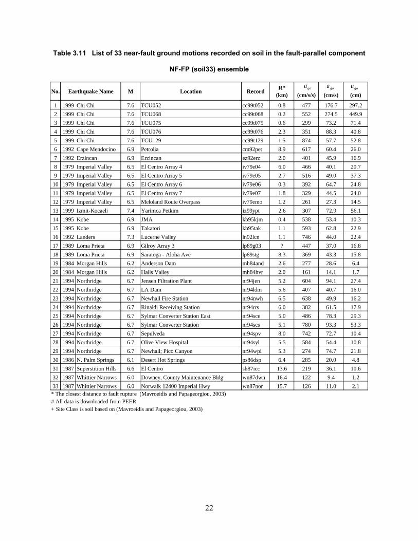
component NF-FN (soil33) ensemble Table 3.11 List of 33 near-fault ground motions recorded on soil in the fault-parallel

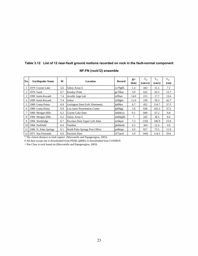
component NF-FP (soil33) ensemble Table 3.12 List of 12 near-fault ground motions recorded on rock in the fault-normal

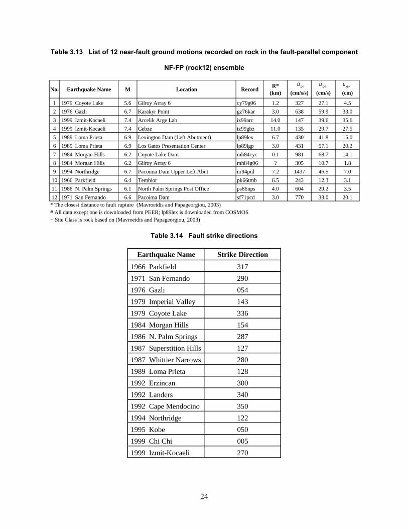
component NF-FN (rock12) ensemble Table 3.13 List of 12 near-fault ground motions recorded on rock in the fault-parallel

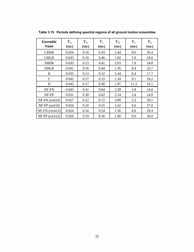
component NF-FP (rock12) ensemble Table 3.14 Fault strike directions Table 3.15 Periods defining spectral regions of all ground motion ensembles

ix

LIST OF FIGURES

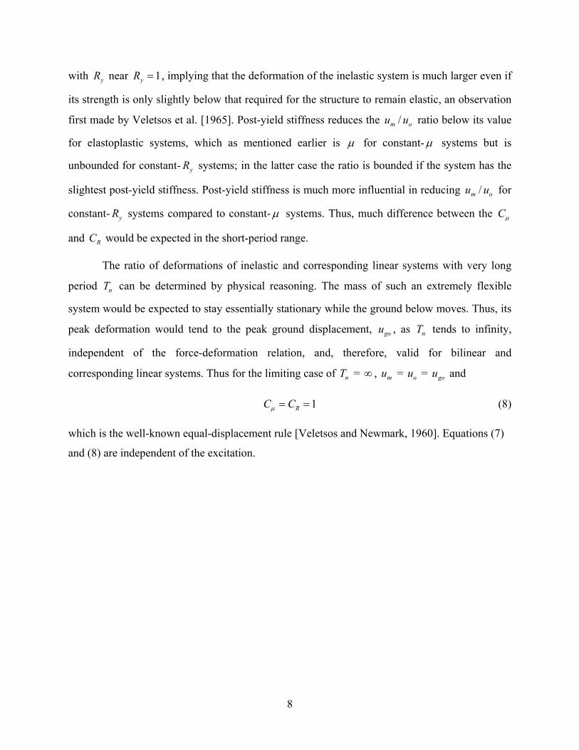
Figure 2.1 Bilinear force-deformation relationship of an inelastic SDF system and the corresponding elastic system.

Figure 2.2 Influence of post-yield stiffness ratio α on limiting values of inelastic deformation ratio as elastic vibration period nT tends to zero: (a) Lµ and (b) RL .

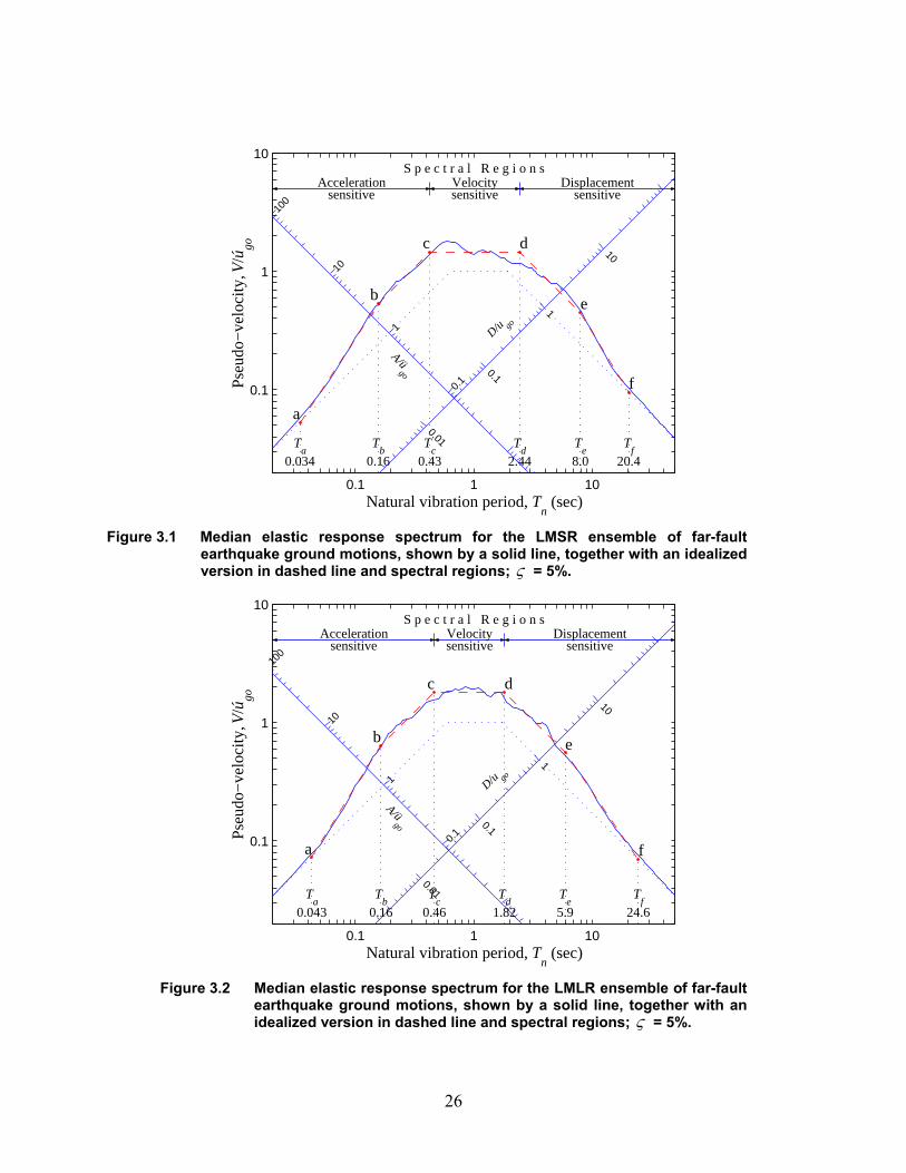
Figure 3.1 Median elastic response spectrum for the LMSR ensemble of far-fault earthquake ground motions, shown by a solid line, together with an idealized version in dashed line and spectral regions; ς = 5%.

Figure 3.2 Median elastic response spectrum for the LMLR ensemble of far-fault earthquake ground motions, shown by a solid line, together with an idealized version in dashed line and spectral regions; ς = 5%.

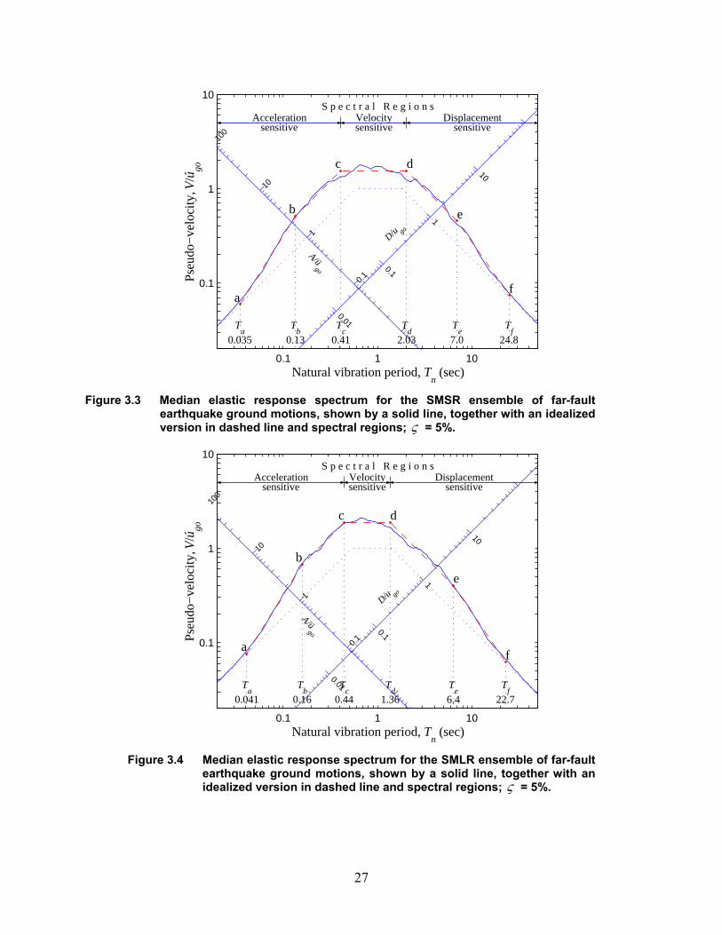
Figure 3.3 Median elastic response spectrum for the SMSR ensemble of far-fault earthquake ground motions, shown by a solid line, together with an idealized version in dashed line and spectral regions; ς = 5%.

Figure 3.4 Median elastic response spectrum for the SMLR ensemble of far-fault earthquake ground motions, shown by a solid line, together with an idealized version in dashed line and spectral regions; ς = 5%.

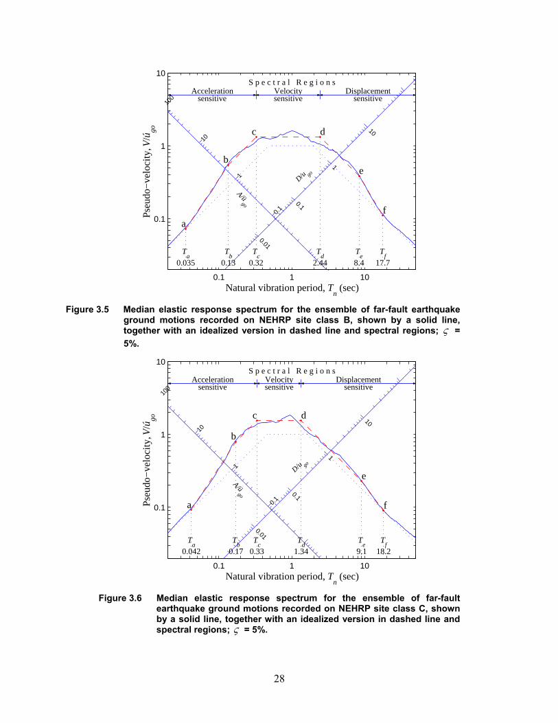
Figure 3.5 Median elastic response spectrum for the ensemble of far-fault earthquake ground motions recorded on NEHRP site class B, shown by a solid line, together with an idealized version in dashed line and spectral regions; ς = 5%.

Figure 3.6 Median elastic response spectrum for the ensemble of far-fault earthquake ground motions recorded on NEHRP site class C, shown by a solid line, together with an idealized version in dashed line and spectral regions; ς = 5%.

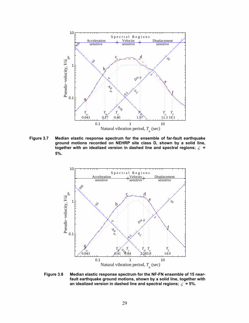
Figure 3.7 Median elastic response spectrum for the ensemble of far-fault earthquake ground motions recorded on NEHRP site class D, shown by a solid line, together with an idealized version in dashed line and spectral regions; ς = 5%.

Figure 3.8 Median elastic response spectrum for the NF-FN ensemble of 15 near-fault earthquake ground motions, shown by a solid line, together with an idealized version in dashed line and spectral regions; ς = 5%.

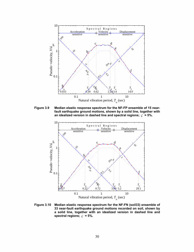
Figure 3.9 Median elastic response spectrum for the NF-FP ensemble of 15 near-fault earthquake ground motions, shown by a solid line, together with an idealized version in dashed line and spectral regions; ς = 5%.

Figure 3.10 Median elastic response spectrum for the NF-FN (soil33) ensemble of 33 near-fault earthquake ground motions recorded on soil, shown by a solid line, together with an idealized version in dashed line and spectral regions; ς = 5%.

x

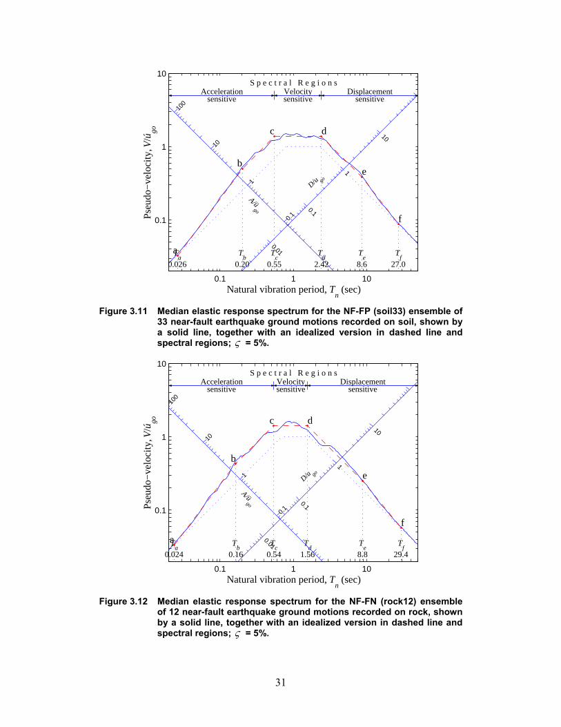
Figure 3.11 Median elastic response spectrum for the NF-FP (soil33) ensemble of 33

near-fault earthquake ground motions recorded on soil, shown by a solid line, together with an idealized version in dashed line and spectral regions; ς = 5%.

Figure 3.12 Median elastic response spectrum for the NF-FN (rock12) ensemble of 12 near-fault earthquake ground motions recorded on rock, shown by a solid line, together with an idealized version in dashed line and spectral regions; ς = 5%.

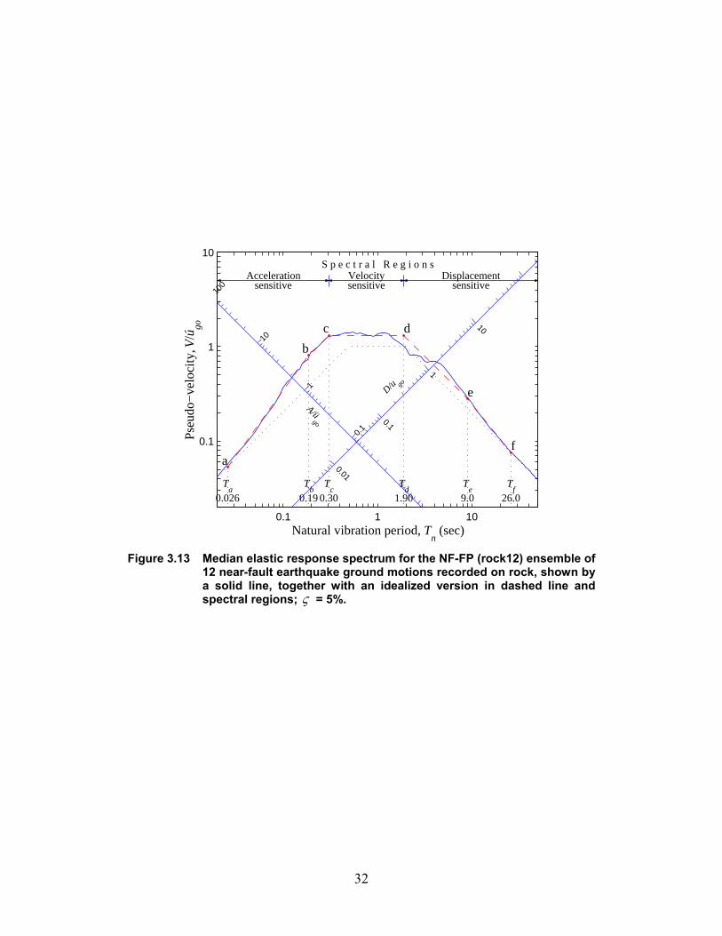
Figure 3.13 Median elastic response spectrum for the NF-FP (rock12) ensemble of 12 near-fault earthquake ground motions recorded on rock, shown by a solid line, together with an idealized version in dashed line and spectral regions; ς = 5%.

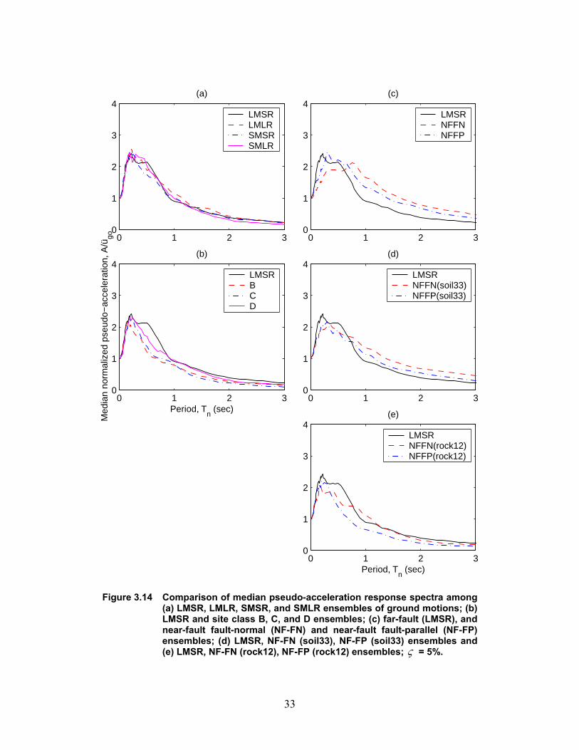
Figure 3.14 Comparison of median pseudo-acceleration response spectra among (a) LMSR, LMLR, SMSR, and SMLR ensembles of ground motions; (b) LMSR and site class B, C, and D ensembles; (c) far-fault (LMSR), and near-fault fault-normal (NF-FN) and near-fault fault-parallel (NF-FP) ensembles; (d) LMSR, NF-FN (soil33), NF-FP (soil33) ensembles and (e) LMSR, NF-FN (rock12), NF-FP (rock12) ensembles; ς = 5%.

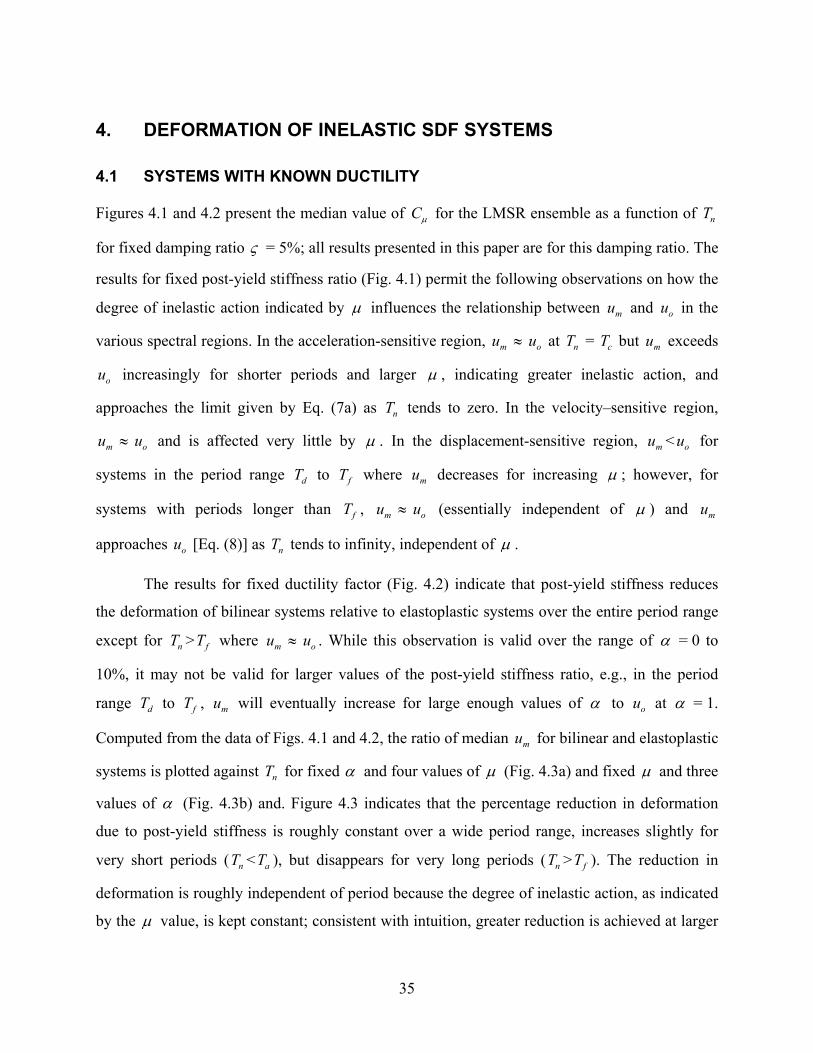
Figure 4.1 Influence of ductility factor µ on the median of inelastic deformation ratio Cµ for bilinear systems (with post-yield stiffness ratioα = 0, 3, 5, and 10%) subjected to the LMSR ensemble of ground motions.

Figure 4.2 Influence of post-yield stiffness ratio α on the median of inelastic deformation ratio Cµ for bilinear systems subjected to the LMSR ensemble of ground motions, presented for fixed values of ductility factor µ =1.5, 2, 4, and 6.

Figure 4.3 Ratio of median deformations mu for bilinear and elastoplastic systems: (a) influence of µ at α = 3% and (b) influence of post-yield stiffness ratio α at ductility factor µ = 4.

Figure 4.4 Dispersion of inelastic deformation ratio Cµ for bilinear systems subjected to the LMSR ensemble of ground motions: (a) influence of ductility factor µ at post-yield stiffness ratio α = 3% and (b) influence of α at µ = 4.

Figure 4.5 Influence of strength reduction factor yR on the median of inelastic deformation ratio RC for bilinear systems (with post-yield stiffness ratio α = 0, 3, 5, and 10%) subjected to the LMSR ensemble of ground motions.

xi

Figure 4.6 Influence of post-yield stiffness ratio α on the median of inelastic deformation ratio RC for bilinear systems subjected to the LMSR ensemble of ground motions for fixed values of strength reduction factor yR = 1.5, 2, 4, and 6.

Figure 4.7 Influence of post-yield stiffness ratio α on (a) ratio of median deformations mu for bilinear and elastoplastic systems and (b) ductility demand for inelastic systems with yR = 4 subjected to the LMSR ensemble of ground motions.

Figure 4.8 Dispersion of inelastic deformation ratio RC for bilinear systems subjected to the LMSR ensemble of ground motions: (a) influence of strength reduction factor yR at post-yield stiffness ratio α = 3% and (b) influence of α at fixed yR = 4.

Figure 5.1 Comparison of inelastic deformation ratio for LMSR, LMLR, SMSR, and SMLR ensembles of far-fault ground motions: (a) Cµ for µ = 4 and α = 3%; (b) RC for yR = 4 and α = 3%.

Figure 5.2 Comparison of inelastic deformation ratio for LMSR and site class B, C, and D ensembles of far-fault ground motions: (a) Cµ for µ = 4 and α = 3%; (b) RC for yR = 4 and α = 3%.

Figure 5.3 Comparison of inelastic deformation ratio Cµ for far-fault LMSR and near-fault ground motions plotted versus (a) elastic vibration period nT and (b) normalized period /n cT T ; both plots are for ductility factor µ = 4 and post-yield stiffness ratio α = 3%.

Figure 5.4 Comparison of inelastic deformation ratio RC for far-fault LMSR and near-fault ground motions plotted versus (a) elastic vibration period nT and (b) normalized period /n cT T ; both plots are for yR = 4 and post-yield stiffness ratio α = 3%.

Figure 6.1 Comparison of mean inelastic deformation ratio Cµ estimated by equations developed by various researchers and LMSR data for ductility factor µ = 6: (a) elastoplastic systems, and (b) post-yield stiffness systems (α =10%).

Figure 6.2 Comparison of median inelastic deformation ratio Cµ estimated by proposed equation with computed data for LMSR-far-fault and near-fault (fault-normal component) ground motions for elastoplastic ( 0α = ) and bilinear ( 10%α = ) systems; and µ = 2 and 6.

xii

Figure 6.3 Comparison of median inelastic deformation ratio Cµ estimated by proposed equation with computed data for LMSR, LMLR, SMSR, and SMLR far-fault ground motions for elastoplastic ( 0α = ) and bilinear ( 10%α = ) systems; and µ = 2 and 6.

Figure 6.4 Comparison of median inelastic deformation ratio Cµ estimated by proposed equation with computed data for far-fault ground motions on site class B, C, and D for elastoplastic ( 0α = ) and bilinear ( 10%α = ) systems; and µ = 2 and 6.

Figure 6.5 Comparison of median inelastic deformation ratio Cµ estimated by proposed equation with computed data for NF-FN and NF-FP near-fault ground motions for elastoplastic ( 0α = ) and bilinear ( 10%α = ) systems; and µ = 2 and 6.

Figure 6.6 Comparison of median inelastic deformation ratio Cµ estimated by proposed equation with computed data for NF-FN (soil33) and NF-FP (soil33) near-fault ground motions for elastoplastic ( 0α = ) and bilinear ( 10%α = ) systems; and µ = 2 and 6.

Figure 6.7 Comparison of median inelastic deformation ratio Cµ estimated by proposed equation with computed data for NF-FN (rock12) and NF-FP (rock12) near-fault ground motions for elastoplastic ( 0α = ) and bilinear ( 10%α = ) systems; and µ = 2 and 6.

Figure 6.8 Comparison of mean inelastic deformation ratio RC estimated by equations developed by various researchers and LMSR data for yR = 4: (a) elastoplastic systems, and (b) bilinear systems (α =10%).

Figure 6.9 Comparison of median inelastic deformation ratio RC estimated by proposed equation with computed data for LMSR-far-fault and near-fault (fault-normal component) ground motions for elastoplastic ( 0α = ) and bilinear ( 10%α = ) systems; and yR = 2 and 6.

Figure 6.10 Comparison of median inelastic deformation ratio RC estimated by proposed equation with computed data for LMSR, LMLR, SMSR, and SMLR far-fault ground motions for elastoplastic ( 0α = ) and bilinear ( 10%α = ) systems; and yR = 2 and 6.

Figure 6.11 Comparison of median inelastic deformation ratio RC estimated by proposed equation with computed data for far-fault ground motions on site class B, C, and D for elastoplastic ( 0α = ) and bilinear ( 10%α = ) systems; and yR = 2 and 6.

xiii

Figure 6.12 Comparison of median inelastic deformation ratio RC estimated by proposed equation with computed data for NF-FN and NF-FP near-fault ground motions for elastoplastic ( 0α = ) and bilinear ( 10%α = ) systems; and yR = 2 and 6.

Figure 6.13 Comparison of median inelastic deformation ratio RC estimated by proposed equation with computed data for NF-FN (soil33) and NF-FP (soil33) near-fault ground motions for elastoplastic ( 0α = ) and bilinear ( 10%α = ) systems; and yR = 2 and 6.

Figure 6.14 Comparison of median inelastic deformation ratio RC estimated by proposed equation with computed data for NF-FN (rock12) and NF-FP (rock12) near-fault ground motions for elastoplastic ( 0α = ) and bilinear ( 10%α = ) systems; and yR = 2 and 6.

1

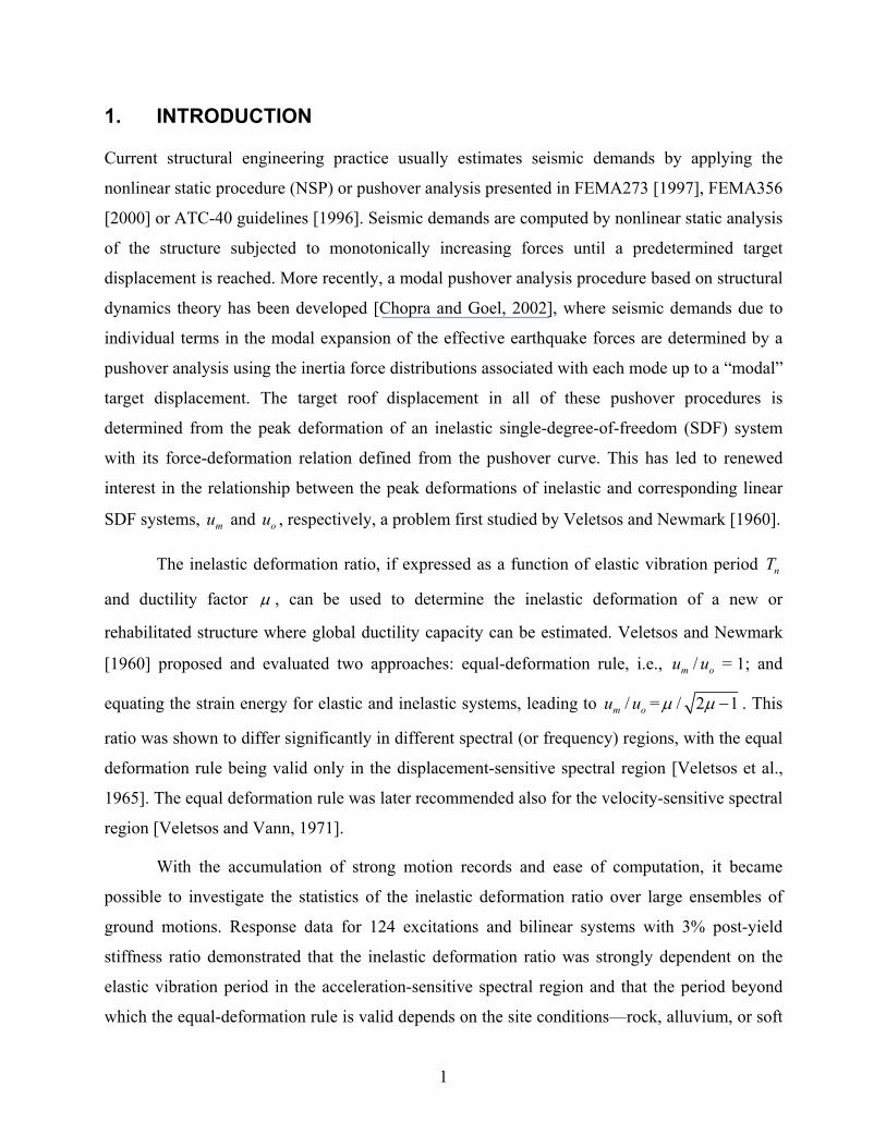
1. INTRODUCTION

Current structural engineering practice usually estimates seismic demands by applying the

nonlinear static procedure (NSP) or pushover analysis presented in FEMA273 [1997], FEMA356

[2000] or ATC-40 guidelines [1996]. Seismic demands are computed by nonlinear static analysis

of the structure subjected to monotonically increasing forces until a predetermined target

displacement is reached. More recently, a modal pushover analysis procedure based on structural

dynamics theory has been developed [Chopra and Goel, 2002], where seismic demands due to

individual terms in the modal expansion of the effective earthquake forces are determined by a

pushover analysis using the inertia force distributions associated with each mode up to a “modal”

target displacement. The target roof displacement in all of these pushover procedures is

determined from the peak deformation of an inelastic single-degree-of-freedom (SDF) system

with its force-deformation relation defined from the pushover curve. This has led to renewed

interest in the relationship between the peak deformations of inelastic and corresponding linear

SDF systems, mu and ou , respectively, a problem first studied by Veletsos and Newmark [1960].

The inelastic deformation ratio, if expressed as a function of elastic vibration period nT

and ductility factor µ , can be used to determine the inelastic deformation of a new or

rehabilitated structure where global ductility capacity can be estimated. Veletsos and Newmark

[1960] proposed and evaluated two approaches: equal-deformation rule, i.e., /m ou u = 1; and

equating the strain energy for elastic and inelastic systems, leading to /m ou u = / 2 1µ µ − . This

ratio was shown to differ significantly in different spectral (or frequency) regions, with the equal

deformation rule being valid only in the displacement-sensitive spectral region [Veletsos et al.,

1965]. The equal deformation rule was later recommended also for the velocity-sensitive spectral

region [Veletsos and Vann, 1971].

With the accumulation of strong motion records and ease of computation, it became

possible to investigate the statistics of the inelastic deformation ratio over large ensembles of

ground motions. Response data for 124 excitations and bilinear systems with 3% post-yield

stiffness ratio demonstrated that the inelastic deformation ratio was strongly dependent on the

elastic vibration period in the acceleration-sensitive spectral region and that the period beyond

which the equal-deformation rule is valid depends on the site conditions—rock, alluvium, or soft

https://www.researchgate.net/publication/227501554_A_modal_pushover_analysis_procedure_for_estimating_seismic_demands_for_buildings?el=1_x_8&enrichId=rgreq-91e216be17565a0c177518e7541077f3-XXX&enrichSource=Y292ZXJQYWdlOzI0NTMwNDg4MDtBUzoxMjkzMTA5NzUzMzY0NDhAMTQwNzg0MTU0NzI0Mw==

2

soil—and on the ductility factor [Miranda, 1991 and 1993]. A more recent investigation based on

264 records concluded that the earthquake magnitude and rupture distance have little influence

on the inelastic deformation ratio [Miranda, 2000]; however, at short periods (0.1 to 1.3 sec), this

ratio for fault-normal near-fault records with forward directivity effects was shown to be much

larger compared to far-fault records [Báez and Miranda, 2000]. Regression analyses of these data

led to an equation, which is restricted to elastoplastic systems, for the inelastic deformation ratio

as a function of elastic vibration period and ductility factor [Miranda, 2000].

The inelastic deformation ratio, if expressed as a function of elastic vibration period and

yield-strength reduction factor yR (= strength required for the structure to remain elastic ÷ yield

strength of the structure), can be used to determine the inelastic deformation of an existing

structure with known lateral strength. For reinforced concrete structures, researchers have

developed an equation that specifies the range of yR and nT where the equal-deformation rule is

valid [Shimazaki and Sozen, 1984], established the short-period range where the inelastic

deformation ratio is sensitive to both strength and stiffness of the system, and developed an

upper bound equation for the deformation [Qi and Moehle, 1991]. An evaluation of the FEMA-

273 procedure for estimating deformation demonstrated that the ratio of the mean inelastic and

elastic deformations exceeds unity if yR exceeds 5, regardless of nT [Whittaker et al., 1998].

Response data for 216 ground motions recorded on NEHRP site classes B, C, and D

demonstrated that the mean inelastic deformation ratio is influenced little by soil condition, by

magnitude if 4yR < (but significantly for larger yR ), or by rupture distance so long as it exceeds

10 km [Ruiz-Garcia and Miranda, 2002]. Regression analysis of these data led to an equation for

the inelastic deformation ratio as a function of nT and yR ; this equation is restricted to

elastoplastic systems.

Researchers have demonstrated that the inelastic deformation ratio in the acceleration-

sensitive spectral region is reduced because of post-yield stiffness [Veletsos, 1969; Qi and

Moehle, 1991], and increased due to stiffness degradation [Clough, 1966; Qi and Moehle, 1991;

Song and Pincheira, 2000] and pinching [Gupta and Kunnath, 1998; Gupta and Krawinkler,

1998; Song and Pincheira, 2000] of the hysteresis loop. However, others have concluded that the

influence of post-yield stiffness on the ductility demand for constant-strength systems is not

https://www.researchgate.net/publication/245304494_Inelastic_Displacement_Ratios_for_Structures_on_Firm_Sites?el=1_x_8&enrichId=rgreq-91e216be17565a0c177518e7541077f3-XXX&enrichSource=Y292ZXJQYWdlOzI0NTMwNDg4MDtBUzoxMjkzMTA5NzUzMzY0NDhAMTQwNzg0MTU0NzI0Mw==


https://www.researchgate.net/publication/37445662_Evaluation_of_Site-Dependent_Inelastic_Seismic_Design_Spectra?el=1_x_8&enrichId=rgreq-91e216be17565a0c177518e7541077f3-XXX&enrichSource=Y292ZXJQYWdlOzI0NTMwNDg4MDtBUzoxMjkzMTA5NzUzMzY0NDhAMTQwNzg0MTU0NzI0Mw==

https://www.researchgate.net/publication/34318251_Seismic_evaluation_and_upgrading_of_existing_buildings?el=1_x_8&enrichId=rgreq-91e216be17565a0c177518e7541077f3-XXX&enrichSource=Y292ZXJQYWdlOzI0NTMwNDg4MDtBUzoxMjkzMTA5NzUzMzY0NDhAMTQwNzg0MTU0NzI0Mw==

3

significant, especially at longer periods [Clough, 1966] and that mean responses of constant-

ductility systems can be conservatively estimated using the elastoplastic model [Riddell et al.,

2002]; it is noticeable—of the order 10-20%—but not predominant on inelastic strength demands

[Nassar and Krawinkler, 1991].

As an alternative to the empirical equations for the inelastic deformation ratio, yR - µ - nT

relations can be used to estimate the peak deformation of an inelastic SDF system [Chopra and

Goel, 1999; Fajfar, 2000], but this indirect method is slightly biased towards underestimating the

deformation [Miranda, 2001].

The objective of this paper is to present the median and dispersion of the inelastic

deformation ratio of SDF systems for several ensembles of ground motions, representing large or

small earthquake magnitude and small or large distance, NEHRP site classes B, C, and D (all

firm sites); near-fault ground motions are also included. Two sets of results are presented, one

for systems with known ductility factor and the other for systems with known yield-strength

reduction factor. The earthquake responses of bilinear systems are investigated comprehensively,

but degradation of stiffness or strength, or pinching of the hysteresis loop is not considered.

Investigated is the influence of earthquake magnitude and distance, site class, and near-fault

ground motions on the inelastic deformation ratio. Presented are two equations—in terms of µ

or yR —for the inelastic deformation ratio, valid for all ground motions ensembles considered, in

a form convenient for application to design or evaluation, respectively, of structures.

https://www.researchgate.net/publication/249872274_A_Nonlinear_Analysis_Method_for_Performance-Based_Seismic_Design?el=1_x_8&enrichId=rgreq-91e216be17565a0c177518e7541077f3-XXX&enrichSource=Y292ZXJQYWdlOzI0NTMwNDg4MDtBUzoxMjkzMTA5NzUzMzY0NDhAMTQwNzg0MTU0NzI0Mw==

https://www.researchgate.net/publication/245606463_Capacity-Demand-Diagram_Methods_Based_on_Inelastic_Design_Spectrum?el=1_x_8&enrichId=rgreq-91e216be17565a0c177518e7541077f3-XXX&enrichSource=Y292ZXJQYWdlOzI0NTMwNDg4MDtBUzoxMjkzMTA5NzUzMzY0NDhAMTQwNzg0MTU0NzI0Mw==


https://www.researchgate.net/publication/246098428_Estimation_of_Inelastic_Deformation_Demands_of_SDOF_Systems?el=1_x_8&enrichId=rgreq-91e216be17565a0c177518e7541077f3-XXX&enrichSource=Y292ZXJQYWdlOzI0NTMwNDg4MDtBUzoxMjkzMTA5NzUzMzY0NDhAMTQwNzg0MTU0NzI0Mw==

https://www.researchgate.net/publication/227594549_Inelastic_deformation_response_of_SDOF_systems_subjected_to_earthquakes?el=1_x_8&enrichId=rgreq-91e216be17565a0c177518e7541077f3-XXX&enrichSource=Y292ZXJQYWdlOzI0NTMwNDg4MDtBUzoxMjkzMTA5NzUzMzY0NDhAMTQwNzg0MTU0NzI0Mw==


https://www.researchgate.net/publication/240232208_Seismic_demands_for_SDOF_and_MDOF_systems?el=1_x_8&enrichId=rgreq-91e216be17565a0c177518e7541077f3-XXX&enrichSource=Y292ZXJQYWdlOzI0NTMwNDg4MDtBUzoxMjkzMTA5NzUzMzY0NDhAMTQwNzg0MTU0NzI0Mw==

5

2. INELASTIC DEFORMATION RATIO: THEORY

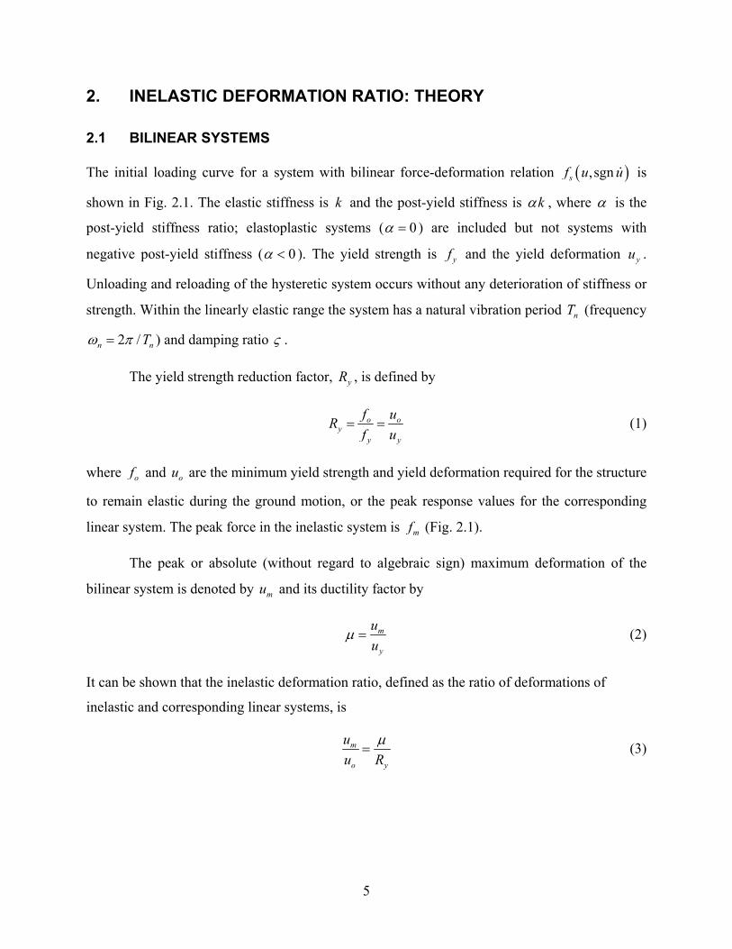
2.1 BILINEAR SYSTEMS

The initial loading curve for a system with bilinear force-deformation relation ( ),sgnsf u u is

shown in Fig. 2.1. The elastic stiffness is k and the post-yield stiffness is kα , where α is the

post-yield stiffness ratio; elastoplastic systems ( 0α = ) are included but not systems with

negative post-yield stiffness ( 0α < ). The yield strength is yf and the yield deformation yu .

Unloading and reloading of the hysteretic system occurs without any deterioration of stiffness or

strength. Within the linearly elastic range the system has a natural vibration period nT (frequency

2 /n nTω π= ) and damping ratio ς .

The yield strength reduction factor, yR , is defined by

o oy

y y

f uRf u

= = (1)

where of and ou are the minimum yield strength and yield deformation required for the structure

to remain elastic during the ground motion, or the peak response values for the corresponding

linear system. The peak force in the inelastic system is mf (Fig. 2.1).

The peak or absolute (without regard to algebraic sign) maximum deformation of the

bilinear system is denoted by mu and its ductility factor by

m

y

uu

µ = (2)

It can be shown that the inelastic deformation ratio, defined as the ratio of deformations of

inelastic and corresponding linear systems, is

m

o y

uu R

µ= (3)

6

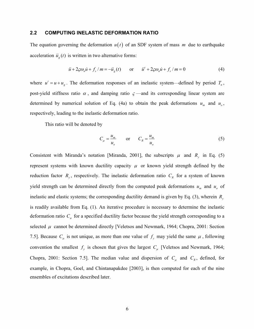
2.2 COMPUTING INELASTIC DEFORMATION RATIO

The equation governing the deformation ( )u t of an SDF system of mass m due to earthquake

acceleration ( )gu t is written in two alternative forms:

2 / ( )n s gu u f m u tςω+ + = − or 2 / 0tn su u f mςω+ + = (4)

where tgu u u= + . The deformation responses of an inelastic system—defined by period nT ,

post-yield stiffness ratio α , and damping ratio ς —and its corresponding linear system are

determined by numerical solution of Eq. (4a) to obtain the peak deformations mu and ou ,

respectively, leading to the inelastic deformation ratio.

This ratio will be denoted by

m

o

uCuµ = or m

Ro

uCu

= (5)

Consistent with Miranda’s notation [Miranda, 2001], the subscripts µ and yR in Eq. (5)

represent systems with known ductility capacity µ or known yield strength defined by the

reduction factor yR , respectively. The inelastic deformation ratio RC for a system of known

yield strength can be determined directly from the computed peak deformations mu and ou of

inelastic and elastic systems; the corresponding ductility demand is given by Eq. (3), wherein yR

is readily available from Eq. (1). An iterative procedure is necessary to determine the inelastic

deformation ratio Cµ for a specified ductility factor because the yield strength corresponding to a

selected µ cannot be determined directly [Veletsos and Newmark, 1964; Chopra, 2001: Section

7.5]. Because Cµ is not unique, as more than one value of yf may yield the same µ , following

convention the smallest yf is chosen that gives the largest Cµ [Veletsos and Newmark, 1964;

Chopra, 2001: Section 7.5]. The median value and dispersion of Cµ and RC , defined, for

example, in Chopra, Goel, and Chintanapakdee [2003], is then computed for each of the nine

ensembles of excitations described later.

7

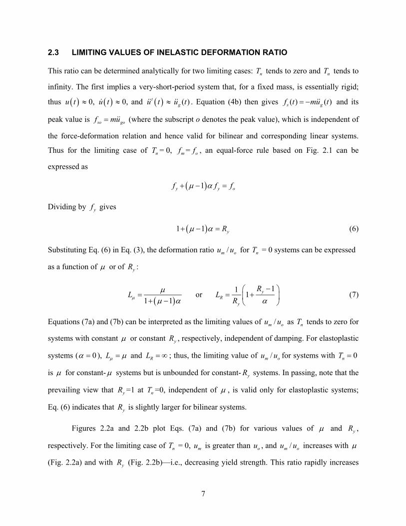
2.3 LIMITING VALUES OF INELASTIC DEFORMATION RATIO

This ratio can be determined analytically for two limiting cases: nT tends to zero and nT tends to

infinity. The first implies a very-short-period system that, for a fixed mass, is essentially rigid;

thus ( )u t ≈ 0, ( )u t ≈ 0, and ( )tu t ≈ ( )gu t . Equation (4b) then gives ( ) ( )s gf t mu t= − and its

peak value is so gof mu= (where the subscript o denotes the peak value), which is independent of

the force-deformation relation and hence valid for bilinear and corresponding linear systems.

Thus for the limiting case of nT = 0, mf = of , an equal-force rule based on Fig. 2.1 can be

expressed as

( )1y y of f fµ α+ − =

Dividing by yf gives

( )1 1 yRµ α+ − = (6)

Substituting Eq. (6) in Eq. (3), the deformation ratio /m ou u for nT = 0 systems can be expressed

as a function of µ or of yR :

( )1 1

Lµµ

µ α=

+ − or

11 1 yR

y

RL

R α−

= +

(7)

Equations (7a) and (7b) can be interpreted as the limiting values of /m ou u as nT tends to zero for

systems with constant µ or constant yR , respectively, independent of damping. For elastoplastic

systems ( 0α = ), Lµ µ= and RL = ∞ ; thus, the limiting value of /m ou u for systems with 0nT =

is µ for constant- µ systems but is unbounded for constant- yR systems. In passing, note that the

prevailing view that yR =1 at nT =0, independent of µ , is valid only for elastoplastic systems;

Eq. (6) indicates that yR is slightly larger for bilinear systems.

Figures 2.2a and 2.2b plot Eqs. (7a) and (7b) for various values of µ and yR ,

respectively. For the limiting case of nT = 0, mu is greater than ou , and /m ou u increases with µ

(Fig. 2.2a) and with yR (Fig. 2.2b)—i.e., decreasing yield strength. This ratio rapidly increases

8

with yR near 1yR = , implying that the deformation of the inelastic system is much larger even if

its strength is only slightly below that required for the structure to remain elastic, an observation

first made by Veletsos et al. [1965]. Post-yield stiffness reduces the /m ou u ratio below its value

for elastoplastic systems, which as mentioned earlier is µ for constant- µ systems but is

unbounded for constant- yR systems; in the latter case the ratio is bounded if the system has the

slightest post-yield stiffness. Post-yield stiffness is much more influential in reducing /m ou u for

constant- yR systems compared to constant- µ systems. Thus, much difference between the Cµ

and RC would be expected in the short-period range.

The ratio of deformations of inelastic and corresponding linear systems with very long

period nT can be determined by physical reasoning. The mass of such an extremely flexible

system would be expected to stay essentially stationary while the ground below moves. Thus, its

peak deformation would tend to the peak ground displacement, gou , as nT tends to infinity,

independent of the force-deformation relation, and, therefore, valid for bilinear and

corresponding linear systems. Thus for the limiting case of nT = ∞ , mu = ou = gou and

1RC Cµ = = (8)

which is the well-known equal-displacement rule [Veletsos and Newmark, 1960]. Equations (7)

and (8) are independent of the excitation.

9

00

fs

u

fy

fm

fo

uy

uo

um

k

αk

Figure 2.1 Bilinear force-deformation relationship of an inelastic SDF system and the corresponding elastic system.

1 2 3 5 101

2

3

5

10

20

30

50

Ductility factor, µ

L µ=u m

/uo a

t Tn=

0

(a)

α=0% α=3% α=5% α=10%

1 2 3 5 101

2

3

5

10

20

30

50

Strength reduction factor, Ry

L R=

u m/u

o at T

n=0

(b)

LR

=∞ for α=0 3%

5%

10%

Figure 2.2 Influence of post-yield stiffness ratio α on limiting values of inelastic deformation ratio as elastic vibration period nT tends to zero: (a) Lµ

and (b) RL .

11

3. GROUND MOTIONS AND ELASTIC RESPONSE SPECTRA

Seven ensembles of far-fault ground motions, each with 20 records, were included in this

investigation. The first group of ensembles, denoted by LMSR, LMLR, SMSR, and SMLR

represent four combinations of large (M = 6.6-6.9) or small (M = 5.8-6.5) magnitude and small

(R = 13-30 km) or large (R = 30-60 km) distance1. These ground motions and their parameters

are tabulated in Tables 3.1 through 3.4. All these records except one correspond to NEHRP site

class D; the Morgan Hill-San Juan Bautista (MH84sjb) record in the SMLR ensemble

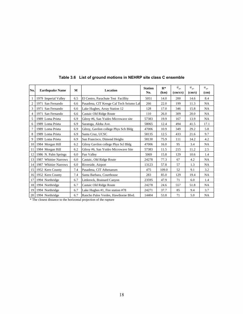
corresponds to NEHRP site class C. The second group of three ensembles is categorized by

NEHRP site classes B, C, or D. These ground motions were recorded during earthquakes with

magnitudes ranging from 6.0 to 7.4 at distances2 ranging from 11 to 118 km; these ground

motions are listed in Tables 3.5 through 3.7.

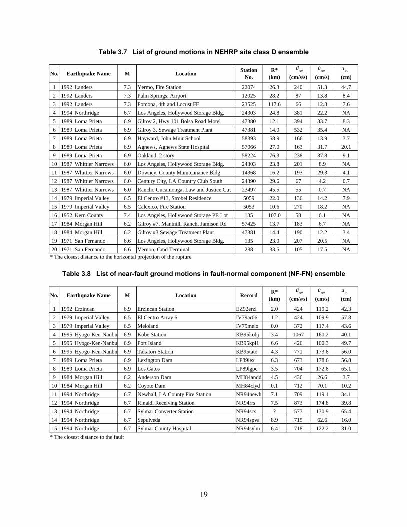
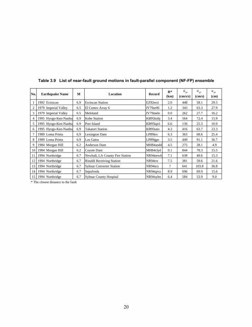
Six ensembles of near-fault ground motions are considered in this study. The first two

ensembles, denoted by NF-FN and NF-FP, are the two horizontal components (fault-normal and

fault-parallel) of 15 near-fault ground motions, recorded during earthquakes of magnitudes

ranging from 6.2 to 6.9 and at distances ranging from 0 to 9 km. These ground motions were all

recorded on firm soil (NEHRP site class D) or rock; the rock motions have been modified to

reproduce soil site conditions [Somerville, 1998]. These two ensembles are listed in Tables 3.8

and 3.9.

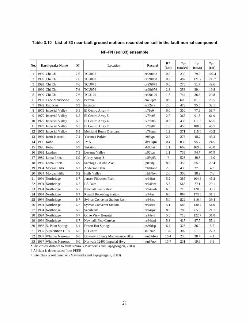
The next two ensembles, denoted by NF-FN (soil33) and NF-FP (soil33), are the fault-

normal and fault-parallel components of 33 near-fault ground motions, all recorded on soil

during earthquakes of magnitudes ranging from 6.0 to 7.6 and at distances ranging from 0.2 to

16.4 km. However, each of these two ensembles includes 11 ground motions from the above set

of 15 near-fault records. These two ensembles are listed in Tables 3.10 and 3.11.

The last two ensembles, denoted by NF-FN (rock12) and NF-FP (rock12), are the fault-

normal and fault-parallel components of 12 near-fault ground motions recorded on rock during

earthquakes of magnitudes ranging from 5.6 to 7.4 and at distances ranging from 0.1 to 14 km.

1 Record-to-source distance is defined as the closest distance to the fault rupture zone except for two records: Point Mugu-Port Hueneme (PM73phn) in the SMSR ensemble and Borrego-El Centro Array#9 (BO42elc) in the SMLR ensemble where the hypocentral distance is reported as 25 and 49 km, respectively. 2 Horizontal distance from the edge of horizontal projection of the fault rupture area to the site.

12

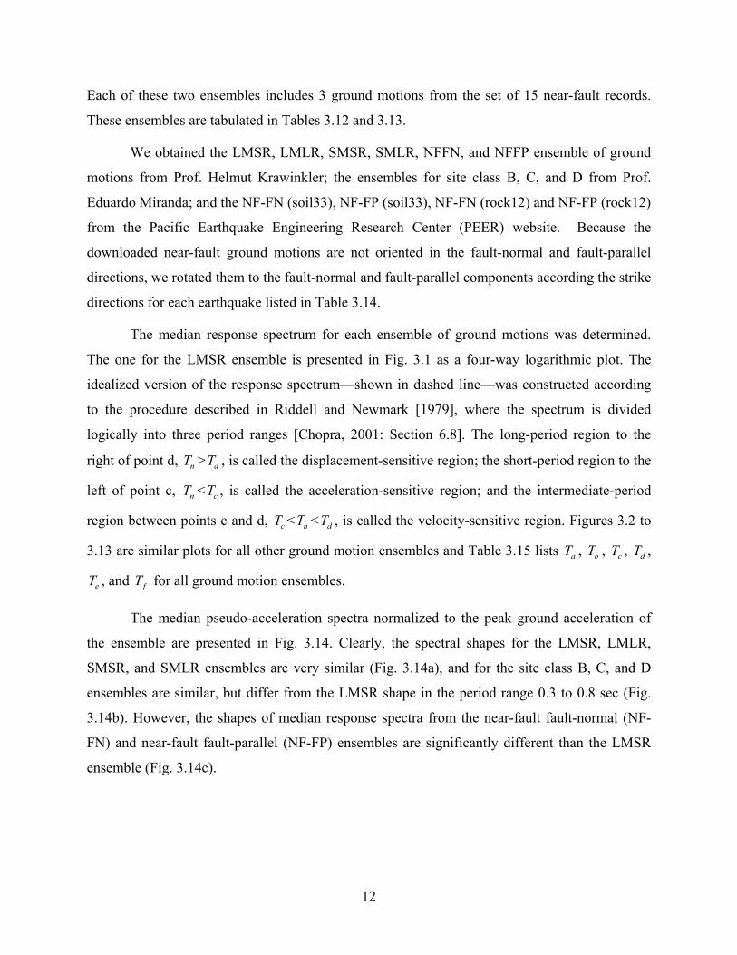
Each of these two ensembles includes 3 ground motions from the set of 15 near-fault records.

These ensembles are tabulated in Tables 3.12 and 3.13.

We obtained the LMSR, LMLR, SMSR, SMLR, NFFN, and NFFP ensemble of ground

motions from Prof. Helmut Krawinkler; the ensembles for site class B, C, and D from Prof.

Eduardo Miranda; and the NF-FN (soil33), NF-FP (soil33), NF-FN (rock12) and NF-FP (rock12)

from the Pacific Earthquake Engineering Research Center (PEER) website. Because the

downloaded near-fault ground motions are not oriented in the fault-normal and fault-parallel

directions, we rotated them to the fault-normal and fault-parallel components according the strike

directions for each earthquake listed in Table 3.14.

The median response spectrum for each ensemble of ground motions was determined.

The one for the LMSR ensemble is presented in Fig. 3.1 as a four-way logarithmic plot. The

idealized version of the response spectrum—shown in dashed line—was constructed according

to the procedure described in Riddell and Newmark [1979], where the spectrum is divided

logically into three period ranges [Chopra, 2001: Section 6.8]. The long-period region to the

right of point d, nT > dT , is called the displacement-sensitive region; the short-period region to the

left of point c, nT < cT , is called the acceleration-sensitive region; and the intermediate-period

region between points c and d, cT < nT < dT , is called the velocity-sensitive region. Figures 3.2 to

3.13 are similar plots for all other ground motion ensembles and Table 3.15 lists aT , bT , cT , dT ,

eT , and fT for all ground motion ensembles.

The median pseudo-acceleration spectra normalized to the peak ground acceleration of

the ensemble are presented in Fig. 3.14. Clearly, the spectral shapes for the LMSR, LMLR,

SMSR, and SMLR ensembles are very similar (Fig. 3.14a), and for the site class B, C, and D

ensembles are similar, but differ from the LMSR shape in the period range 0.3 to 0.8 sec (Fig.

3.14b). However, the shapes of median response spectra from the near-fault fault-normal (NF-

FN) and near-fault fault-parallel (NF-FP) ensembles are significantly different than the LMSR

ensemble (Fig. 3.14c).

13

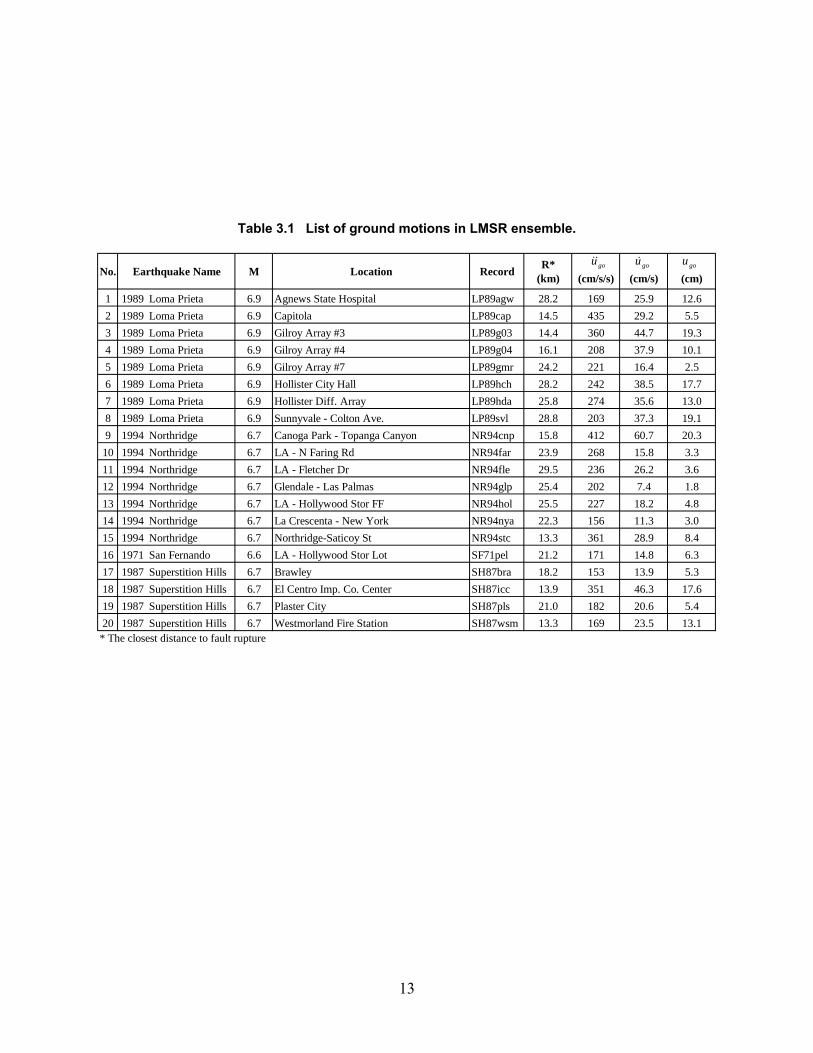
Table 3.1 List of ground motions in LMSR ensemble.

No. Earthquake Name M Location RecordR*

(km)

(cm/s/s)

(cm/s)

(cm)

1 1989 Loma Prieta 6.9 Agnews State Hospital LP89agw 28.2 169 25.9 12.6

2 1989 Loma Prieta 6.9 Capitola LP89cap 14.5 435 29.2 5.5

3 1989 Loma Prieta 6.9 Gilroy Array #3 LP89g03 14.4 360 44.7 19.3


5 1989 Loma Prieta 6.9 Gilroy Array #7 LP89gmr 24.2 221 16.4 2.5

6 1989 Loma Prieta 6.9 Hollister City Hall LP89hch 28.2 242 38.5 17.7

7 1989 Loma Prieta 6.9 Hollister Diff. Array LP89hda 25.8 274 35.6 13.0

8 1989 Loma Prieta 6.9 Sunnyvale - Colton Ave. LP89svl 28.8 203 37.3 19.1

9 1994 Northridge 6.7 Canoga Park - Topanga Canyon NR94cnp 15.8 412 60.7 20.3

10 1994 Northridge 6.7 LA - N Faring Rd NR94far 23.9 268 15.8 3.3

11 1994 Northridge 6.7 LA - Fletcher Dr NR94fle 29.5 236 26.2 3.6

12 1994 Northridge 6.7 Glendale - Las Palmas NR94glp 25.4 202 7.4 1.8

13 1994 Northridge 6.7 LA - Hollywood Stor FF NR94hol 25.5 227 18.2 4.8

14 1994 Northridge 6.7 La Crescenta - New York NR94nya 22.3 156 11.3 3.0

15 1994 Northridge 6.7 Northridge-Saticoy St NR94stc 13.3 361 28.9 8.4

16 1971 San Fernando 6.6 LA - Hollywood Stor Lot SF71pel 21.2 171 14.8 6.3

17 1987 Superstition Hills 6.7 Brawley SH87bra 18.2 153 13.9 5.3

18 1987 Superstition Hills 6.7 El Centro Imp. Co. Center SH87icc 13.9 351 46.3 17.6

19 1987 Superstition Hills 6.7 Plaster City SH87pls 21.0 182 20.6 5.4

20 1987 Superstition Hills 6.7 Westmorland Fire Station SH87wsm 13.3 169 23.5 13.1* The closest distance to fault rupture

gou gou gou

14

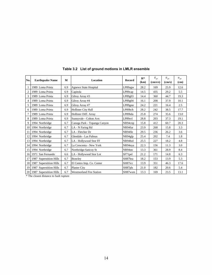
Table 3.2 List of ground motions in LMLR ensemble


(km)

(cm/s/s)

(cm/s)

(cm)

1 1989 Loma Prieta 6.9 Agnews State Hospital LP89agw 28.2 169 25.9 12.6

2 1989 Loma Prieta 6.9 Capitola LP89cap 14.5 435 29.2 5.5



5 1989 Loma Prieta 6.9 Gilroy Array #7 LP89gmr 24.2 221 16.4 2.5

6 1989 Loma Prieta 6.9 Hollister City Hall LP89hch 28.2 242 38.5 17.7

7 1989 Loma Prieta 6.9 Hollister Diff. Array LP89hda 25.8 274 35.6 13.0

8 1989 Loma Prieta 6.9 Sunnyvale - Colton Ave. LP89svl 28.8 203 37.3 19.1

9 1994 Northridge 6.7 Canoga Park - Topanga Canyon NR94cnp 15.8 412 60.7 20.3

10 1994 Northridge 6.7 LA - N Faring Rd NR94far 23.9 268 15.8 3.3

11 1994 Northridge 6.7 LA - Fletcher Dr NR94fle 29.5 236 26.2 3.6

12 1994 Northridge 6.7 Glendale - Las Palmas NR94glp 25.4 202 7.4 1.8

13 1994 Northridge 6.7 LA - Hollywood Stor FF NR94hol 25.5 227 18.2 4.8

14 1994 Northridge 6.7 La Crescenta - New York NR94nya 22.3 156 11.3 3.0

15 1994 Northridge 6.7 Northridge-Saticoy St NR94stc 13.3 361 28.9 8.4

16 1971 San Fernando 6.6 LA - Hollywood Stor Lot SF71pel 21.2 171 14.8 6.3

17 1987 Superstition Hills 6.7 Brawley SH87bra 18.2 153 13.9 5.3

18 1987 Superstition Hills 6.7 El Centro Imp. Co. Center SH87icc 13.9 351 46.3 17.6

19 1987 Superstition Hills 6.7 Plaster City SH87pls 21.0 182 20.6 5.4

20 1987 Superstition Hills 6.7 Westmorland Fire Station SH87wsm 13.3 169 23.5 13.1* The closest distance to fault rupture

gou gou gou

15

Table 3.3 List of ground motions in SMSR ensemble


(km)

(cm/s/s)

(cm/s)

(cm)

1 1979 Imperial Valley 6.5 Calipatria Fire Station IV79cal 23.8 77 13.3 6.2

2 1979 Imperial Valley 6.5 Chihuahua IV79chi 28.7 265 24.8 9.1

3 1979 Imperial Valley 6.5 El Centro Array #1 IV79e01 15.5 137 15.8 10.0



6 1979 Imperial Valley 6.5 Cucapah IV79qkp 23.6 303 36.3 10.7

7 1979 Imperial Valley 6.5 Westmorland Fire Station IV79wsm 15.1 108 21.9 10.0

8 1980 Livermore 5.8 San Ramon - Eastman Kodak LV80kod 17.6 75 6.1 1.7

9 1980 Livermore 5.8 San Ramon Fire Station LV80srm 21.7 39 4.0 1.2

10 1984 Morgan Hill 6.2 Agnews State Hospital MH84agw 29.4 31 5.5 2.0

11 1984 Morgan Hill 6.2 Gilroy Array #2 MH84g02 15.1 159 5.1 1.4

12 1984 Morgan Hill 6.2 Gilroy Array #3 MH84g03 14.6 191 11.2 2.4

13 1984 Morgan Hill 6.2 Gilroy Array #7 MH84gmr 14.0 111 6.0 1.8

14 1973 Point Mugu 5.8 Port Hueneme PM73phn NA 110 14.8 2.6

15 1986 N. Palm Springs 6.0 Palm Springs Airport PS86psa 16.6 184 12.1 2.1

16 1987 Whittier Narrows 6.0 Compton - Castlegate St WN87cas 16.9 325 27.1 5.0

17 1987 Whittier Narrows 6.0 Carson - Catskill Ave WN87cat 28.1 41 3.8 0.8

18 1987 Whittier Narrows 6.0 Brea - S Flower Av WN87flo 17.9 113 7.0 1.2

19 1987 Whittier Narrows 6.0 LA - W 70th St WN87w70 16.3 148 8.6 1.5

20 1987 Whittier Narrows 6.0 Carson - Water St WN87wat 24.5 102 9.0 1.9* The closest distance to fault rupture

gou gou gou

16

Table 3.4 List of ground motions in SMLR ensemble


(km)

(cm/s/s)

(cm/s)

(cm)

1 1942 Borrego Mountain NA El Centro Array #9 BO42elc NA 67 3.9 1.4

2 1983 Coalinga 6.4 Parkfield - Cholame 5W CO83c05 47.3 128 9.9 1.3

3 1983 Coalinga 6.4 Parkfield - Cholame 8W CO83c08 50.7 96 8.5 1.5

4 1979 Imperial Valley 6.5 Coachella Canal #4 IV79cc4 49.3 126 15.6 3.0

5 1979 Imperial Valley 6.5 Compuertas IV79cmp 32.6 183 13.8 2.9

6 1979 Imperial Valley 6.5 Delta IV79dlt 43.6 233 26.0 12.0

7 1979 Imperial Valley 6.5 Niland Fire Station IV79nil 35.9 107 11.9 6.9

8 1979 Imperial Valley 6.5 Plaster City IV79pls 31.7 56 5.4 1.9

9 1979 Imperial Valley 6.5 Victoria IV79vct 54.1 163 8.3 1.0

10 1980 Livermore 5.8 Tracy - Sewage Treatment Plant LV80stp 37.3 72 7.6 1.8

11 1984 Morgan Hill 6.2 Capitola MH84cap 38.1 97 4.9 0.6

12 1984 Morgan Hill 6.2 Hollister City Hall MH84hch 32.5 70 7.4 1.6

13 1984 Morgan Hill 6.2 San Juan Bautista MH84sjb 30.3 35 4.4 1.5

14 1986 N. Palm Springs 6.0 San Jacinto Valley Cem PS86h06 39.6 62 4.4 1.2

15 1986 N. Palm Springs 6.0 Indio PS86ino 39.6 63 6.6 2.2

16 1987 Whittier Narrows 6.0 Downey - Birchdale WN87bir 56.8 293 37.6 4.9

17 1987 Whittier Narrows 6.0 LA - Century City CC South WN87cts 31.3 51 3.5 0.6

18 1987 Whittier Narrows 6.0 LB - Harbor Admin FF WN87har 34.2 70 7.3 0.9

19 1987 Whittier Narrows 6.0 Terminal Island - S Seaside WN87sse 35.7 41 3.9 1.0

20 1987 Whittier Narrows 6.0 Northridge - Saticoy St WN87stc 39.8 115 5.1 0.8* The closest distance to fault rupture

gou gou gou

17

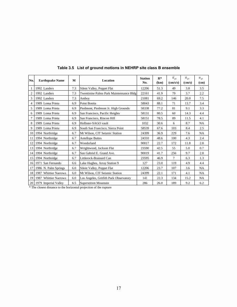
Table 3.5 List of ground motions in NEHRP site class B ensemble

No. Earthquake Name M LocationStation

No.R*

(km)

(cm/s/s)

(cm/s)

(cm)

1 1992 Landers 7.3 Silent Valley, Poppet Flat 12206 51.3 49 3.8 3.5

2 1992 Landers 7.3 Twentinine Palms Park Maintennance Bldg 22161 41.9 79 3.7 2.2

3 1992 Landers 7.3 Amboy 21081 69.2 146 20.0 7.5

4 1989 Loma Prieta 6.9 Point Bonita 58043 88.1 71 13.7 3.4

5 1989 Loma Prieta 6.9 Piedmont, Piedmont Jr. High Grounds 58338 77.2 81 9.1 3.3

6 1989 Loma Prieta 6.9 San Francisco, Pacific Heights 58131 80.5 60 14.3 4.4

7 1989 Loma Prieta 6.9 San Francisco, Rincon Hill 58151 78.5 89 11.5 4.1

8 1989 Loma Prieta 6.9 Hollister-SAGO vault 1032 30.6 6 8.7 NA

9 1989 Loma Prieta 6.9 South San Francisco, Sierra Point 58539 67.6 103 8.4 2.5

10 1994 Northridge 6.7 Mt Wilson, CIT Seismic Station 24399 36.9 229 7.6 NA

11 1994 Northridge 6.7 Antellope Buttes 24310 48.6 100 4.3 2.4

12 1994 Northridge 6.7 Wonderland 90017 22.7 172 11.8 2.8

13 1994 Northridge 6.7 Wrightwood, Jackson Flat 23590 42.5 55 5.0 0.7

14 1994 Northridge 6.7 San Gabriel E. Grand Ave. 90019 41.7 256 9.7 2.8

15 1994 Northridge 6.7 Littlerock-Brainard Can 23595 46.9 7 6.3 1.3

16 1971 San Fernando 6.6 Lake Hughes, Array Station 9 127 23.0 119 4.9 4.4

17 1986 N. Palm Springs 6.0 Silent Valley, Poppet Flat 12206 23.7 107 3.6 NA

18 1987 Whittier Narrows 6.0 Mt Wilson, CIT Seismic Station 24399 22.1 171 4.1 NA

19 1987 Whittier Narrows 6.0 Los Angeles, Gritfith Park Observatory 141 22.3 134 15.2 NA

20 1979 Imperial Valley 6.5 Superstition Mountain 286 26.0 189 9.2 6.2* The closest distance to the horizontal projection of the rupture

gou gou gou

18

Table 3.6 List of ground motions in NEHRP site class C ensemble


No.R*

(km)

(cm/s/s)

(cm/s)

(cm)

1 1979 Imperial Valley 6.5 El Centro, Parachute Test Facillity 5051 14.0 200 14.6 8.4

2 1971 San Fernando 6.6Pasadena, CIT Kresge Cal Tech Seismo Lab 266 22.0 199 11.3 NA

3 1971 San Fernando 6.6 Lake Hughes, Array Station 12 128 17.0 346 15.8 NA

4 1971 San Fernando 6.6 Castaic Old Ridge Route 110 26.0 309 20.0 NA

5 1989 Loma Prieta 6.9 Gilroy #6, San Ysidro Microwave site 57383 19.9 167 13.9 NA

6 1989 Loma Prieta 6.9 Saratoga, Aloha Ave. 58065 12.4 494 41.5 17.1

7 1989 Loma Prieta 6.9 Gilroy, Gavilon college Phys Sch Bldg 47006 10.9 349 29.2 5.8

8 1989 Loma Prieta 6.9 Santa Cruz, UCSC 58135 12.5 433 21.6 9.7

9 1989 Loma Prieta 6.9 San Francisco, Dimond Heighs 58130 75.9 111 14.2 4.2

10 1984 Morgan Hill 6.2 Gilroy Gavilon college Phys Scl Bldg 47006 16.0 95 3.4 NA

11 1984 Morgan Hill 6.2 Gilroy #6, San Ysidro Microwave Site 57383 11.5 215 11.2 2.5

12 1986 N. Palm Springs 6.0 Fun Valley 5069 15.8 129 10.6 1.4

13 1987 Whittier Narrows 6.0 Castaic, Old Ridge Route 24278 77.3 67 4.2 NA

14 1987 Whittier Narrows 6.0 Riverside, Airport 13123 57.8 57 1.3 NA

15 1952 Kern County 7.4 Pasadena, CIT Athenaeum 475 109.0 52 9.1 3.2

16 1952 Kern County 7.4 Santa Barbara, Courthouse 283 85.0 129 19.4 NA

17 1994 Northridge 6.7 Littlerock, Brainard Canyon 23595 47.9 71 6.0 1.4

18 1994 Northridge 6.7 Castaic Old Ridge Route 24278 24.6 557 51.8 NA

19 1994 Northridge 6.7 Lake Hughes #1, Fire station #78 24271 37.7 85 9.4 3.7

20 1994 Northridge 6.7 Rancho Palos Verdes, Hawthorne Blvd. 14404 53.8 71 5.0 NA* The closest distance to the horizontal projection of the rupture

gou gou gou

19

Table 3.7 List of ground motions in NEHRP site class D ensemble


No.R*

(km)

(cm/s/s)

(cm/s)

(cm)

1 1992 Landers 7.3 Yermo, Fire Station 22074 26.3 240 51.3 44.7

2 1992 Landers 7.3 Palm Springs, Airport 12025 28.2 87 13.8 8.4

3 1992 Landers 7.3 Pomona, 4th and Locust FF 23525 117.6 66 12.8 7.6

4 1994 Northridge 6.7 Los Angeles, Hollywood Storage Bldg. 24303 24.8 381 22.2 NA

5 1989 Loma Prieta 6.9 Gilroy 2, Hwy 101 Bolsa Road Motel 47380 12.1 394 33.7 8.3

6 1989 Loma Prieta 6.9 Gilroy 3, Sewage Treatment Plant 47381 14.0 532 35.4 NA

7 1989 Loma Prieta 6.9 Hayward, John Muir School 58393 58.9 166 13.9 3.7

8 1989 Loma Prieta 6.9 Agnews, Agnews State Hospital 57066 27.0 163 31.7 20.1

9 1989 Loma Prieta 6.9 Oakland, 2 story 58224 76.3 238 37.8 9.1

10 1987 Whittier Narrows 6.0 Los Angeles, Hollywood Storage Bldg. 24303 23.8 201 8.9 NA

11 1987 Whittier Narrows 6.0 Downey, County Maintennance Bldg 14368 16.2 193 29.3 4.1

12 1987 Whittier Narrows 6.0 Century City, LA Country Club South 24390 29.6 67 4.2 0.7

13 1987 Whittier Narrows 6.0 Rancho Cucamonga, Law and Justice Ctr. 23497 45.5 55 0.7 NA

14 1979 Imperial Valley 6.5 El Centro #13, Strobel Residence 5059 22.0 136 14.2 7.9

15 1979 Imperial Valley 6.5 Calexico, Fire Station 5053 10.6 270 18.2 NA

16 1952 Kern County 7.4 Los Angeles, Hollywood Storage PE Lot 135 107.0 58 6.1 NA

17 1984 Morgan Hill 6.2 Gilroy #7, Mantnilli Ranch, Jamison Rd 57425 13.7 183 6.7 NA

18 1984 Morgan Hill 6.2 Gilroy #3 Sewage Treatment Plant 47381 14.4 190 12.2 3.4

19 1971 San Fernando 6.6 Los Angeles, Hollywood Storage Bldg. 135 23.0 207 20.5 NA

20 1971 San Fernando 6.6 Vernon, Cmd Terminal 288 33.5 105 17.5 NA* The closest distance to the horizontal projection of the rupture

gou gou gou

Table 3.8 List of near-fault ground motions in fault-normal component (NF-FN) ensemble


(km)

(cm/s/s)

(cm/s)

(cm)

1 1992 Erzincan 6.9 Erzincan Station EZ92erzi 2.0 424 119.2 42.3

2 1979 Imperial Valley 6.5 El Centro Array 6 IV79ar06 1.2 424 109.9 57.8

3 1979 Imperial Valley 6.5 Meloland IV79melo 0.0 372 117.4 43.6

4 1995 Hyogo-Ken-Nanbu 6.9 Kobe Station KB95kobj 3.4 1067 160.2 40.1

5 1995 Hyogo-Ken-Nanbu 6.9 Port Island KB95kpi1 6.6 426 100.3 49.7

6 1995 Hyogo-Ken-Nanbu 6.9 Takatori Station KB95tato 4.3 771 173.8 56.0

7 1989 Loma Prieta 6.9 Lexington Dam LP89lex 6.3 673 178.6 56.8

8 1989 Loma Prieta 6.9 Los Gatos LP89lgpc 3.5 704 172.8 65.1

9 1984 Morgan Hill 6.2 Anderson Dam MH84andd 4.5 436 26.6 3.7

10 1984 Morgan Hill 6.2 Coyote Dam MH84clyd 0.1 712 70.1 10.2

11 1994 Northridge 6.7 Newhall, LA County Fire Station NR94newh 7.1 709 119.1 34.1

12 1994 Northridge 6.7 Rinaldi Receiving Station NR94rrs 7.5 873 174.8 39.8

13 1994 Northridge 6.7 Sylmar Converter Station NR94scs ? 577 130.9 65.4

14 1994 Northridge 6.7 Sepulveda NR94spva 8.9 715 62.6 16.0

15 1994 Northridge 6.7 Sylmar County Hospital NR94sylm 6.4 718 122.2 31.0

* The closest distance to the fault

gou gou gou

20

Table 3.9 List of near-fault ground motions in fault-parallel component (NF-FP) ensemble


(km)

(cm/s/s)

(cm/s)

(cm)

1 1992 Erzincan 6.9 Erzincan Station EZ92erzi 2.0 448 58.1 29.5

2 1979 Imperial Valley 6.5 El Centro Array 6 IV79ar06 1.2 343 63.3 27.9

3 1979 Imperial Valley 6.5 Meloland IV79melo 0.0 262 27.7 16.2

4 1995 Hyogo-Ken-Nanbu 6.9 Kobe Station KB95kobj 3.4 564 72.4 15.9

5 1995 Hyogo-Ken-Nanbu 6.9 Port Island KB95kpi1 6.6 136 25.3 10.0

6 1995 Hyogo-Ken-Nanbu 6.9 Takatori Station KB95tato 4.3 416 63.7 23.3

7 1989 Loma Prieta 6.9 Lexington Dam LP89lex 6.3 363 68.6 25.4

8 1989 Loma Prieta 6.9 Los Gatos LP89lgpc 3.5 449 91.1 36.7

9 1984 Morgan Hill 6.2 Anderson Dam MH84andd 4.5 275 28.1 4.9

10 1984 Morgan Hill 6.2 Coyote Dam MH84clyd 0.1 844 78.3 15.5

11 1994 Northridge 6.7 Newhall, LA County Fire Station NR94newh 7.1 638 49.6 15.3

12 1994 Northridge 6.7 Rinaldi Receiving Station NR94rrs 7.5 381 59.6 21.6

13 1994 Northridge 6.7 Sylmar Converter Station NR94scs ? 641 103.8 36.8

14 1994 Northridge 6.7 Sepulveda NR94spva 8.9 696 69.9 15.6

15 1994 Northridge 6.7 Sylmar County Hospital NR94sylm 6.4 584 53.9 9.0

* The closest distance to the fault

gou gou gou

21

Table 3.10 List of 33 near-fault ground motions recorded on soil in the fault-normal component

NF-FN (soil33) ensemble


(km)

(cm/s/s)

(cm/s)

(cm)

1 1999 Chi Chi 7.6 TCU052 cc99t052 0.8 230 79.9 102.4

2 1999 Chi Chi 7.6 TCU068 cc99t068 0.2 487 121.7 196.7

3 1999 Chi Chi 7.6 TCU075 cc99t075 0.6 278 51.7 49.6

4 1999 Chi Chi 7.6 TCU076 cc99t076 2.3 353 39.4 19.8

5 1999 Chi Chi 7.6 TCU129 cc99t129 1.5 744 36.6 29.8

6 1992 Cape Mendocino 6.9 Petrolia cm92pet 8.9 603 81.8 25.5

7 1992 Erzincan 6.9 Erzincan ez92erz 2.0 479 95.5 32.1

8 1979 Imperial Valley 6.5 El Centro Array 4 iv79e04 6.0 350 77.8 58.7




12 1979 Imperial Valley 6.5 Meloland Route Overpass iv79emo 1.2 371 115.0 40.2

13 1999 Izmit-Kocaeli 7.4 Yarimca Petkim iz99ypt 2.6 273 48.2 43.2

14 1995 Kobe 6.9 JMA kb95kjm 0.4 838 95.7 24.5

15 1995 Kobe 6.9 Takatori kb95tak 1.1 669 169.5 45.0

16 1992 Landers 7.3 Lucerne Valley ln92lcn 1.1 739 94.7 67.9

17 1989 Loma Prieta 6.9 Gilroy Array 3 lp89g03 ? 523 49.3 11.0

18 1989 Loma Prieta 6.9 Saratoga - Aloha Ave lp89stg 8.3 356 55.5 29.4

19 1984 Morgan Hills 6.2 Anderson Dam mh84and 2.6 430 27.3 4.3

20 1984 Morgan Hills 6.2 Halls Valley mh84hvr 2.0 300 38.9 7.6

21 1994 Northridge 6.7 Jensen Filtration Plant nr94jen 5.2 385 104.3 45.2

22 1994 Northridge 6.7 LA Dam nr94ldm 5.6 565 77.1 20.1

23 1994 Northridge 6.7 Newhall Fire Station nr94nwh 6.5 710 120.0 35.1

24 1994 Northridge 6.7 Rinaldi Receiving Station nr94rrs 6.0 869 173.0 31.1

25 1994 Northridge 6.7 Sylmar Converter Station East nr94sce 5.0 822 116.4 39.4

26 1994 Northridge 6.7 Sylmar Converter Station nr94scs 5.1 583 130.2 54.0

27 1994 Northridge 6.7 Sepulveda nr94spv 8.0 708 65.0 21.1

28 1994 Northridge 6.7 Olive View Hospital nr94syl 5.5 718 122.7 31.8

29 1994 Northridge 6.7 Newhall; Pico Canyon nr94wpi 5.3 417 87.7 55.1

30 1986 N. Palm Springs 6.1 Desert Hot Springs ps86dsp 6.4 323 26.9 5.7

31 1987 Superstition Hills 6.6 El Centro sh87icc 13.6 302 51.9 22.2

32 1987 Whittier Narrows 6.0 Downey, County Maintenance Bldg wn87dwn 16.4 230 30.4 4.1

33 1987 Whittier Narrows 6.0 Norwalk 12400 Imperial Hwy wn87nor 15.7 231 19.8 3.9* The closest distance to fault rupture (Mavroeidis and Papageorgiou, 2003)# All data is downloaded from PEER+ Site Class is soil based on (Mavroeidis and Papageorgiou, 2003)

gou gou gou

22

Table 3.11 List of 33 near-fault ground motions recorded on soil in the fault-parallel component

NF-FP (soil33) ensemble


(km)

(cm/s/s)

(cm/s)

(cm)

1 1999 Chi Chi 7.6 TCU052 cc99t052 0.8 477 176.7 297.2

2 1999 Chi Chi 7.6 TCU068 cc99t068 0.2 552 274.5 449.9

3 1999 Chi Chi 7.6 TCU075 cc99t075 0.6 299 73.2 71.4

4 1999 Chi Chi 7.6 TCU076 cc99t076 2.3 351 88.3 40.8

5 1999 Chi Chi 7.6 TCU129 cc99t129 1.5 874 57.7 52.8

6 1992 Cape Mendocino 6.9 Petrolia cm92pet 8.9 617 60.4 26.0

7 1992 Erzincan 6.9 Erzincan ez92erz 2.0 401 45.9 16.9





12 1979 Imperial Valley 6.5 Meloland Route Overpass iv79emo 1.2 261 27.3 14.5

13 1999 Izmit-Kocaeli 7.4 Yarimca Petkim iz99ypt 2.6 307 72.9 56.1

14 1995 Kobe 6.9 JMA kb95kjm 0.4 538 53.4 10.3

15 1995 Kobe 6.9 Takatori kb95tak 1.1 593 62.8 22.9

16 1992 Landers 7.3 Lucerne Valley ln92lcn 1.1 746 44.0 22.4

17 1989 Loma Prieta 6.9 Gilroy Array 3 lp89g03 ? 447 37.0 16.8

18 1989 Loma Prieta 6.9 Saratoga - Aloha Ave lp89stg 8.3 369 43.3 15.8

19 1984 Morgan Hills 6.2 Anderson Dam mh84and 2.6 277 28.6 6.4

20 1984 Morgan Hills 6.2 Halls Valley mh84hvr 2.0 161 14.1 1.7

21 1994 Northridge 6.7 Jensen Filtration Plant nr94jen 5.2 604 94.1 27.4

22 1994 Northridge 6.7 LA Dam nr94ldm 5.6 407 40.7 16.0

23 1994 Northridge 6.7 Newhall Fire Station nr94nwh 6.5 638 49.9 16.2

24 1994 Northridge 6.7 Rinaldi Receiving Station nr94rrs 6.0 382 61.5 17.9

25 1994 Northridge 6.7 Sylmar Converter Station East nr94sce 5.0 486 78.3 29.3

26 1994 Northridge 6.7 Sylmar Converter Station nr94scs 5.1 780 93.3 53.3

27 1994 Northridge 6.7 Sepulveda nr94spv 8.0 742 72.7 10.4

28 1994 Northridge 6.7 Olive View Hospital nr94syl 5.5 584 54.4 10.8

29 1994 Northridge 6.7 Newhall; Pico Canyon nr94wpi 5.3 274 74.7 21.8

30 1986 N. Palm Springs 6.1 Desert Hot Springs ps86dsp 6.4 285 20.0 4.8

31 1987 Superstition Hills 6.6 El Centro sh87icc 13.6 219 36.1 10.6

32 1987 Whittier Narrows 6.0 Downey, County Maintenance Bldg wn87dwn 16.4 122 9.4 1.2

33 1987 Whittier Narrows 6.0 Norwalk 12400 Imperial Hwy wn87nor 15.7 126 11.0 2.1* The closest distance to fault rupture (Mavroeidis and Papageorgiou, 2003)# All data is downloaded from PEER+ Site Class is soil based on (Mavroeidis and Papageorgiou, 2003)

gou gou gou

23

Table 3.12 List of 12 near-fault ground motions recorded on rock in the fault-normal component

NF-FN (rock12) ensemble


(km)

(cm/s/s)

(cm/s)

(cm)

1 1979 Coyote Lake 5.6 Gilroy Array 6 cy79g06 1.2 443 51.5 7.1

2 1976 Gazli 6.7 Karakyr Point gz76kar 3.0 622 62.5 13.7

3 1999 Izmit-Kocaeli 7.4 Arcelik Arge Lab iz99arc 14.0 215 17.7 13.6

4 1999 Izmit-Kocaeli 7.4 Gebze iz99gbz 11.0 239 50.3 42.7

5 1989 Loma Prieta 6.9 Lexington Dam (Left Abutment) lp89lex 6.7 452 114.7 37.5

6 1989 Loma Prieta 6.9 Los Gatos Presentation Center lp89lgp 3.0 636 102.3 37.2

7 1984 Morgan Hills 6.2 Coyote Lake Dam mh84cyc 0.1 849 67.2 9.8

8 1984 Morgan Hills 6.2 Gilroy Array 6 mh84g06 ? 245 36.5 6.6

9 1994 Northridge 6.7 Pacoima Dam Upper Left Abut nr94pul 7.2 1350 106.9 23.0

10 1966 Parkfield 6.4 Temblor pk66tmb 6.5 364 22.4 4.6

11 1986 N. Palm Springs 6.1 North Palm Springs Post Office ps86nps 4.0 657 73.5 11.9

12 1971 San Fernando 6.6 Pacoima Dam sf71pcd 3.0 1443 114.3 29.6* The closest distance to fault rupture (Mavroeidis and Papageorgiou, 2003)# All data except one is downloaded from PEER; lp89lex is downloaded from COSMOS+ Site Class is rock based on (Mavroeidis and Papageorgiou, 2003)

gou gou gou

24

Table 3.13 List of 12 near-fault ground motions recorded on rock in the fault-parallel component

NF-FP (rock12) ensemble


(km)

(cm/s/s)

(cm/s)

(cm)

1 1979 Coyote Lake 5.6 Gilroy Array 6 cy79g06 1.2 327 27.1 4.5

2 1976 Gazli 6.7 Karakyr Point gz76kar 3.0 638 59.9 33.0

3 1999 Izmit-Kocaeli 7.4 Arcelik Arge Lab iz99arc 14.0 147 39.6 35.6

4 1999 Izmit-Kocaeli 7.4 Gebze iz99gbz 11.0 135 29.7 27.5

5 1989 Loma Prieta 6.9 Lexington Dam (Left Abutment) lp89lex 6.7 430 41.8 15.0

6 1989 Loma Prieta 6.9 Los Gatos Presentation Center lp89lgp 3.0 431 57.1 20.2

7 1984 Morgan Hills 6.2 Coyote Lake Dam mh84cyc 0.1 981 68.7 14.1

8 1984 Morgan Hills 6.2 Gilroy Array 6 mh84g06 ? 305 10.7 1.8

9 1994 Northridge 6.7 Pacoima Dam Upper Left Abut nr94pul 7.2 1437 46.5 7.0

10 1966 Parkfield 6.4 Temblor pk66tmb 6.5 243 12.3 3.1

11 1986 N. Palm Springs 6.1 North Palm Springs Post Office ps86nps 4.0 604 29.2 3.5

12 1971 San Fernando 6.6 Pacoima Dam sf71pcd 3.0 770 38.0 20.1* The closest distance to fault rupture (Mavroeidis and Papageorgiou, 2003)# All data except one is downloaded from PEER; lp89lex is downloaded from COSMOS+ Site Class is rock based on (Mavroeidis and Papageorgiou, 2003)

gou gou gou

Table 3.14 Fault strike directions

Earthquake Name Strike Direction

1966 Parkfield 317

1971 San Fernando 290

1976 Gazli 054

1979 Imperial Valley 143

1979 Coyote Lake 336

1984 Morgan Hills 154

1986 N. Palm Springs 287

1987 Superstition Hills 127

1987 Whittier Narrows 280

1989 Loma Prieta 128

1992 Erzincan 300

1992 Landers 340

1992 Cape Mendocino 350

1994 Northridge 122

1995 Kobe 050

1999 Chi Chi 005

1999 Izmit-Kocaeli 270

25

Table 3.15 Periods defining spectral regions of all ground motion ensembles

EnsembleName

T a

(sec)T b

(sec)T c

(sec)T d

(sec)T e

(sec)T f

(sec)

LMSR 0.034 0.16 0.43 2.44 8.0 20.4

LMLR 0.043 0.16 0.46 1.82 5.9 24.6

SMSR 0.035 0.13 0.41 2.03 7.0 24.8

SMLR 0.041 0.16 0.44 1.36 6.4 22.7

B 0.035 0.13 0.32 2.44 8.4 17.7

C 0.042 0.17 0.33 1.34 9.1 18.2

D 0.043 0.17 0.40 1.97 11.3 19.1

NF-FN 0.043 0.41 0.84 2.58 3.8 14.0

NF-FP 0.031 0.30 0.62 2.24 3.4 14.0

NF-FN (soil33) 0.027 0.22 0.72 3.09 5.2 29.1

NF-FP (soil33) 0.026 0.20 0.55 2.42 8.6 27.0

NF-FN (rock12) 0.024 0.16 0.54 1.56 8.8 29.4

NF-FP (rock12) 0.026 0.19 0.30 1.90 9.0 26.0

26

0.1 1 10

0.1

1

10

Pse

udo−

velo

city

, V/ú

go

Natural vibration period, Tn (sec)

D/u go

A/ügo

0.1

1

10

100

0.01

0.1

1

10

Ta

0.034T

b0.16

Tc

0.43T

d2.44

Te

8.0T

f20.4

S p e c t r a l R e g i o n sAcceleration Velocity Displacement

sensitive sensitive sensitive

a

b

c d

e

f

Figure 3.1 Median elastic response spectrum for the LMSR ensemble of far-fault

earthquake ground motions, shown by a solid line, together with an idealized version in dashed line and spectral regions; ς = 5%.

0.1 1 10

0.1

1

10

Pse

udo−

velo

city

, V/ú

go


D/u go

A/ügo

0.1

1

10

100

0.01

0.1

1

10

Ta

0.043T

b0.16

Tc

0.46T

d1.82

Te

5.9T

f24.6



a

b

c d

e

f

Figure 3.2 Median elastic response spectrum for the LMLR ensemble of far-fault


27

0.1 1 10

0.1

1

10

Pse

udo−

velo

city

, V/ú

go


D/u go

A/ügo

0.1

1

10

100

0.01

0.1

1

10

Ta

0.035T

b0.13

Tc

0.41T

d2.03

Te

7.0T

f24.8



a

b

c d

e

f

Figure 3.3 Median elastic response spectrum for the SMSR ensemble of far-fault


0.1 1 10

0.1

1

10

Pse

udo−

velo

city

, V/ú

go


D/u go

A/ügo

0.1

1

10

100

0.01

0.1

1

10

Ta

0.041T

b0.16

Tc

0.44T

d1.36

Te

6.4T

f22.7



a

b

c d

e

f

Figure 3.4 Median elastic response spectrum for the SMLR ensemble of far-fault


28

0.1 1 10

0.1

1

10

Pse

udo−

velo

city

, V/ú

go


D/u go

A/ügo

0.1

1

10

100

0.01

0.1

1

10

Ta

0.035T

b0.13

Tc

0.32T

d2.44

Te

8.4T

f17.7



a

b

c d

e

f

Figure 3.5 Median elastic response spectrum for the ensemble of far-fault earthquake

ground motions recorded on NEHRP site class B, shown by a solid line, together with an idealized version in dashed line and spectral regions; ς = 5%.

0.1 1 10

0.1

1

10

Pse

udo−

velo

city

, V/ú

go


D/u go

A/ügo

0.1

1

10

100

0.01

0.1

1

10

Ta

0.042T

b0.17

Tc

0.33T

d1.34

Te

9.1T

f18.2



a

b

c d

e

f

Figure 3.6 Median elastic response spectrum for the ensemble of far-fault

earthquake ground motions recorded on NEHRP site class C, shown by a solid line, together with an idealized version in dashed line and spectral regions; ς = 5%.

29

0.1 1 10

0.1

1

10

Pse

udo−

velo

city

, V/ú

go


D/u go

A/ügo

0.1

1

10

100

0.01

0.1

1

10

Ta

0.043T

b0.17

Tc

0.40T

d1.97

Te

11.3T

f19.1



a

b

c d

e

f

Figure 3.7 Median elastic response spectrum for the ensemble of far-fault earthquake

ground motions recorded on NEHRP site class D, shown by a solid line, together with an idealized version in dashed line and spectral regions; ς = 5%.

0.1 1 10

0.1

1

10

Pse

udo−

velo

city

, V/ú

go


D/u go

A/ügo

0.1

1

10

100

0.01

0.1

1

10

Ta

0.043T

b0.41

Tc

0.84T

d2.58

Te

3.8T

f14.0



a

b

c de

f

Figure 3.8 Median elastic response spectrum for the NF-FN ensemble of 15 near-

fault earthquake ground motions, shown by a solid line, together with an idealized version in dashed line and spectral regions; ς = 5%.

30

0.1 1 10

0.1

1

10

Pse

udo−

velo

city

, V/ú

go


D/u go

A/ügo

0.1

1

10

100

0.01

0.1

1

10

Ta

0.031T

b0.30

Tc

0.62T

d2.24

Te

3.4T

f14.0



a

b

c de

f

Figure 3.9 Median elastic response spectrum for the NF-FP ensemble of 15 near-

fault earthquake ground motions, shown by a solid line, together with an idealized version in dashed line and spectral regions; ς = 5%.

0.1 1 10

0.1

1

10

Pse

udo−

velo

city

, V/ú

go


D/u go

A/ügo

0.1

1

10

100

0.01

0.1

1

10

Ta

0.027T

b0.22

Tc

0.72T

d3.09

Te

5.2T

f29.1



a

b

c d

e

f

Figure 3.10 Median elastic response spectrum for the NF-FN (soil33) ensemble of

33 near-fault earthquake ground motions recorded on soil, shown by a solid line, together with an idealized version in dashed line and spectral regions; ς = 5%.

31

0.1 1 10

0.1

1

10

Pse

udo−

velo

city

, V/ú

go


D/u go

A/ügo

0.1

1

10

100

0.01

0.1

1

10

Ta

0.026T

b0.20

Tc

0.55T

d2.42

Te

8.6T

f27.0



a

b

c d

e

f

Figure 3.11 Median elastic response spectrum for the NF-FP (soil33) ensemble of

33 near-fault earthquake ground motions recorded on soil, shown by a solid line, together with an idealized version in dashed line and spectral regions; ς = 5%.

0.1 1 10

0.1

1

10

Pse

udo−

velo

city

, V/ú

go


D/u go

A/ügo

0.1

1

10

100

0.01

0.1

1

10

Ta

0.024T

b0.16

Tc

0.54T

d1.56

Te

8.8T

f29.4



a

b

c d

e

f

Figure 3.12 Median elastic response spectrum for the NF-FN (rock12) ensemble

of 12 near-fault earthquake ground motions recorded on rock, shown by a solid line, together with an idealized version in dashed line and spectral regions; ς = 5%.

32

0.1 1 10

0.1

1

10

Pse

udo−

velo

city

, V/ú

go


D/u go

A/ügo

0.1

1

10

100

0.01

0.1

1

10

Ta

0.026T

b0.19

Tc

0.30T

d1.90

Te

9.0T

f26.0



a

b

c d

e

f

Figure 3.13 Median elastic response spectrum for the NF-FP (rock12) ensemble of

12 near-fault earthquake ground motions recorded on rock, shown by a solid line, together with an idealized version in dashed line and spectral regions; ς = 5%.

33

0 1 2 30

1

2

3

4(a)

LMSRLMLRSMSRSMLR

0 1 2 30

1

2

3

4

Med

ian

norm

aliz

ed p

seud

o−ac

cele

ratio

n, A

/ügo

Period, Tn (sec)

(b)

LMSRB C D

0 1 2 30

1

2

3

4(c)

LMSRNFFNNFFP

0 1 2 30

1

2

3

4(d)

LMSR NFFN(soil33)NFFP(soil33)

0 1 2 30

1

2

3

4

Period, Tn (sec)

(e)

LMSR NFFN(rock12)NFFP(rock12)

Figure 3.14 Comparison of median pseudo-acceleration response spectra among (a) LMSR, LMLR, SMSR, and SMLR ensembles of ground motions; (b) LMSR and site class B, C, and D ensembles; (c) far-fault (LMSR), and near-fault fault-normal (NF-FN) and near-fault fault-parallel (NF-FP) ensembles; (d) LMSR, NF-FN (soil33), NF-FP (soil33) ensembles and (e) LMSR, NF-FN (rock12), NF-FP (rock12) ensembles; ς = 5%.

35

4. DEFORMATION OF INELASTIC SDF SYSTEMS

4.1 SYSTEMS WITH KNOWN DUCTILITY

Figures 4.1 and 4.2 present the median value of Cµ for the LMSR ensemble as a function of nT

for fixed damping ratio ς = 5%; all results presented in this paper are for this damping ratio. The

results for fixed post-yield stiffness ratio (Fig. 4.1) permit the following observations on how the

degree of inelastic action indicated by µ influences the relationship between mu and ou in the

various spectral regions. In the acceleration-sensitive region, mu ≈ ou at nT = cT but mu exceeds

ou increasingly for shorter periods and larger µ , indicating greater inelastic action, and

approaches the limit given by Eq. (7a) as nT tends to zero. In the velocity–sensitive region,

mu ≈ ou and is affected very little by µ . In the displacement-sensitive region, mu < ou for

systems in the period range dT to fT where mu decreases for increasing µ ; however, for

systems with periods longer than fT , mu ≈ ou (essentially independent of µ ) and mu

approaches ou [Eq. (8)] as nT tends to infinity, independent of µ .

The results for fixed ductility factor (Fig. 4.2) indicate that post-yield stiffness reduces

the deformation of bilinear systems relative to elastoplastic systems over the entire period range

except for nT > fT where mu ≈ ou . While this observation is valid over the range of α = 0 to

10%, it may not be valid for larger values of the post-yield stiffness ratio, e.g., in the period

range dT to fT , mu will eventually increase for large enough values of α to ou at α = 1.

Computed from the data of Figs. 4.1 and 4.2, the ratio of median mu for bilinear and elastoplastic

systems is plotted against nT for fixed α and four values of µ (Fig. 4.3a) and fixed µ and three

values of α (Fig. 4.3b) and. Figure 4.3 indicates that the percentage reduction in deformation

due to post-yield stiffness is roughly constant over a wide period range, increases slightly for

very short periods ( nT < aT ), but disappears for very long periods ( nT > fT ). The reduction in

deformation is roughly independent of period because the degree of inelastic action, as indicated

by the µ value, is kept constant; consistent with intuition, greater reduction is achieved at larger

36

ductility factors. The reduction of deformation due to post-yield stiffness is modest for realistic

values of α and µ ; e.g., for µ = 4 and α = 3% the deformation is reduced by less than 15%

over the entire period range (Fig. 4.3a). These results support the view that for systems with

known and small ductility, elastoplastic models provide a usefully conservative estimate of

deformation [Riddell and Newmark, 1979; Riddell et al., 2002] and is consistent with the earlier

result that yR is affected little by post-yield stiffness [Nassar and Krawinkler, 1991].

The dispersion of Cµ for the LMSR ensemble is plotted against nT for fixed α and four

values of µ (Fig. 4.4a) and for fixed µ with four values of α (Fig. 4.4b). Here the dispersion is

(1) zero as nT tends to zero or infinity because the limiting value of Cµ [Eqs. (7a) and (8)] is

independent of the ground motion; (2) roughly similar over a wide range of periods from bT to

eT ; (3) increases with µ (Fig. 4.4a) consistent with intuition; and (4) affected very little by post-

yield stiffness over the range of α considered (Fig4.4b), contrary to intuition.

4.2 SYSTEMS WITH KNOWN yR

Figures 4.5 and 4.6 present the median value of RC for the LMSR ensemble as a function of nT

for 5%ς = . The results for fixed post-yield stiffness ratio (Fig. 4.5) permit the following

observations on how the yield strength influences the relationship between the deformations mu

and ou of inelastic and elastic systems in the various spectral regions. In the acceleration-

sensitive region, starting from mu ≈ ou at nT = cT , mu exceeds ou increasingly for shorter

periods where mu is very sensitive to the yield strength, increasing as the yield strength is

reduced; mu approaches the limit given by Eq. (7b) as nT tends to zero. Very short period

systems ( nT < aT ), even systems with strength only slightly smaller than the minimum strength

required for the systems to remain elastic (e.g., yR = 1.5), experience deformations much larger

than the elastic deformation. Just as in the case of constant- µ systems, mu ≈ ou in the velocity-

sensitive region and is essentially independent of the yield strength. In the displacement-sensitive

region, the relationship between mu and ou is similar to that observed for constant- µ systems:

mu < ou for systems in the period range dT to fT where mu decreases as strength is reduced;


https://www.researchgate.net/publication/39066852_Statistical_Analysis_of_the_Response_of_Nonlinear_Systems_Subjected_to_Earthquakes?el=1_x_8&enrichId=rgreq-91e216be17565a0c177518e7541077f3-XXX&enrichSource=Y292ZXJQYWdlOzI0NTMwNDg4MDtBUzoxMjkzMTA5NzUzMzY0NDhAMTQwNzg0MTU0NzI0Mw==


37

mu ≈ ou , essentially independent of strength, for periods longer than fT ; and mu approaches ou

[Eq. (8)] as nT tends to infinity, independent of yield strength. The results for fixed (or constant)

yR presented in Fig. 4.6 indicates that post-yield stiffness reduces the deformation of a bilinear

system relative to its value for elastoplastic systems.

Although the deformation is reduced over the entire period range, the ratio of median mu

for bilinear and elastoplastic systems demonstrates that post-yield stiffness reduces the

deformation only moderately in the velocity and displacement-sensitive regions; e.g. for 4yR =

and nT > cT this reduction is less than 13%, 17%, and 22% for α = 3, 5, and 10%, respectively

(Fig. 4.7a). In these regions, the percentage reduction in deformation due to post-yield stiffness is

insensitive to the period because the median ductility demand is roughly constant over this

period range (Fig. 4.7b). However, the deformation is reduced considerably in the acceleration-

sensitive region, especially for periods shorter than bT .

The constant- yR plots in Fig. 4.7a demonstrate that post-yield stiffness is much more

effective in reducing deformation in the acceleration-sensitive region than observed from the

constant- µ plots of Fig. 4.3a. Such is the case because ductility demands for systems with a

selected yR (say, 4yR = ) are much larger than the yR (say, 4) value in the acceleration-sensitive

spectral region (Fig. 4.7b); and larger µ implies larger reduction in deformation due to post-

yield stiffness (Fig. 4.3b). This observation implies that ignoring post-yield stiffness in

estimating deformation is too conservative for seismic evaluation of existing structures with

periods in the acceleration-sensitive region. While factual and seemingly significant, this

observation may not be important for real structures because they are usually strong enough to

remain elastic for most ground motions.

The dispersion of RC for the LMSR ensemble is plotted against nT for fixed α and four

values of yR (Fig. 4.8a) and for fixed yR with four values of α (Fig. 4.8b). Here the dispersion

is: (1) zero as nT tends to zero (except for elastoplastic systems, 0α = , Fig. 4.8b) or as nT tends

to infinity because the limiting values of RC [Eqs. (7b) and (8)] are independent of the ground

motion; (2) larger for weaker (larger yR ) systems over a wide range of periods except for nT < bT

38

where this trend is reversed; (3) essentially independent of post-yield stiffness ratio (Fig. 4.8b)

for periods in the velocity and displacement-sensitive regions; and (4) reduced significantly with

the slightest post-yield stiffness in the very short-period ( nT < bT ) portion of the acceleration-

sensitive region.

39

0.01 0.1 1 10 1000.5

1

2

3

5

10

Med

ian

Cµ

(a) α=0%

Ta

Tb

Tc

Td

Te

Tf

µ=1.5µ=2 µ=4 µ=6

0.01 0.1 1 10 1000.5

1

2

3

5

10(b) α=3%

Ta

Tb

Tc

Td

Te

Tf

0.01 0.1 1 10 1000.5

1

2

3

5

10(c) α=5%

Period, Tn (sec)

Med

ian

Cµ

Ta

Tb

Tc

Td

Te

Tf

0.01 0.1 1 10 1000.5

1

2

3

5

10(d) α=10%

Period, Tn (sec)

Ta

Tb

Tc

Td

Te

Tf

Figure 4.1 Influence of ductility factor µ on the median of inelastic deformation ratio Cµ for bilinear systems (with post-yield stiffness ratioα = 0, 3, 5, and 10%) subjected to the LMSR ensemble of ground motions.

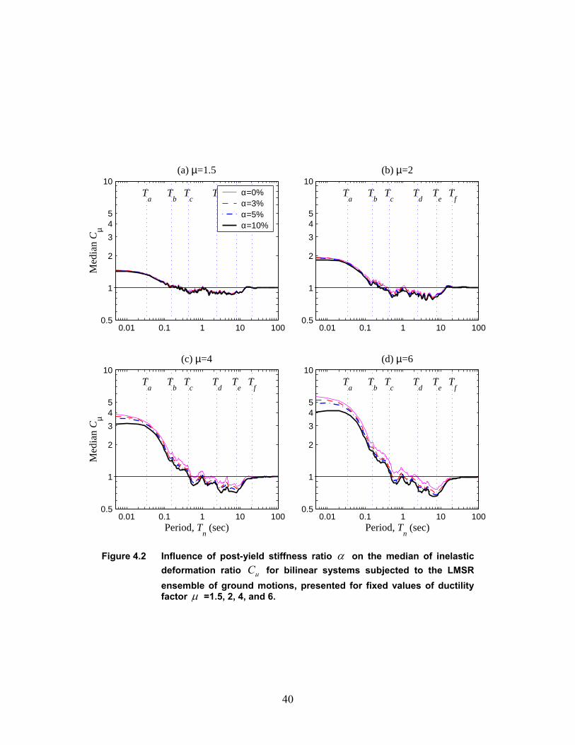
40

0.01 0.1 1 10 1000.5

1

2

3

45

10(a) µ=1.5

Med

ian

Cµ

Ta

Tb

Tc

Td

Te

Tf

α=0% α=3% α=5% α=10%

0.01 0.1 1 10 1000.5

1

2

3

45

10(b) µ=2

Ta

Tb

Tc

Td

Te

Tf

0.01 0.1 1 10 1000.5

1

2

3

45

10(c) µ=4

Period, Tn (sec)

Med

ian

Cµ

Ta

Tb

Tc

Td

Te

Tf

0.01 0.1 1 10 1000.5

1

2

3

45

10(d) µ=6

Period, Tn (sec)

Ta

Tb

Tc

Td

Te

Tf

Figure 4.2 Influence of post-yield stiffness ratio α on the median of inelastic deformation ratio Cµ for bilinear systems subjected to the LMSR ensemble of ground motions, presented for fixed values of ductility factor µ =1.5, 2, 4, and 6.

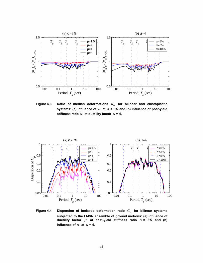
41

0.01 0.1 1 10 1000.5

1

1.5(b) µ=4

Period, Tn (sec)

(um) α÷(

u m) α=

0%

Ta

Tb

Tc

Td

Te

Tf

α=3% α=5% α=10%

0.01 0.1 1 10 1000.5

1

1.5(a) α=3%

Period, Tn (sec)

(um) α÷(

u m) α=

0%

Ta

Tb

Tc

Td

Te

Tf

µ=1.5µ=2 µ=4 µ=6

Figure 4.3 Ratio of median deformations mu for bilinear and elastoplastic systems: (a) influence of µ at α = 3% and (b) influence of post-yield stiffness ratio α at ductility factor µ = 4.

0.01 0.1 1 10 1000.05

0.1

0.2

0.3

0.5

1

Period, Tn (sec)

Dis

pers

ion

of C

µ

(a) α=3%

Ta

Tb

Tc

Td

Te

Tf

µ=1.5µ=2 µ=4 µ=6

0.01 0.1 1 10 1000.05

0.1

0.2

0.3

0.5

1(b) µ=4

Period, Tn (sec)

Ta

Tb

Tc

Td

Te

Tf

α=0% α=3% α=5% α=10%

Figure 4.4 Dispersion of inelastic deformation ratio Cµ for bilinear systems subjected to the LMSR ensemble of ground motions: (a) influence of ductility factor µ at post-yield stiffness ratio α = 3% and (b) influence of α at µ = 4.

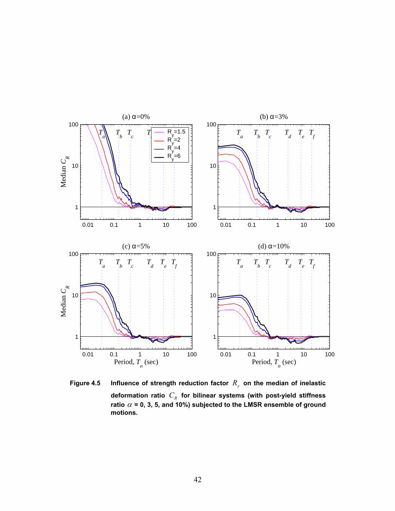
42

0.01 0.1 1 10 100

1

10

100(a) α=0%

Med

ian

CR

Ta

Tb

Tc

Td

Te

Tf

Ry=1.5

Ry=2

Ry=4

Ry=6

0.01 0.1 1 10 100

1

10

100(b) α=3%

Ta

Tb

Tc

Td

Te

Tf

0.01 0.1 1 10 100

1

10

100(c) α=5%

Period, Tn (sec)

Med

ian

CR

Ta

Tb

Tc

Td

Te

Tf

0.01 0.1 1 10 100

1

10

100(d) α=10%

Period, Tn (sec)

Ta

Tb

Tc

Td

Te

Tf

Figure 4.5 Influence of strength reduction factor yR on the median of inelastic

deformation ratio RC for bilinear systems (with post-yield stiffness ratio α = 0, 3, 5, and 10%) subjected to the LMSR ensemble of ground motions.

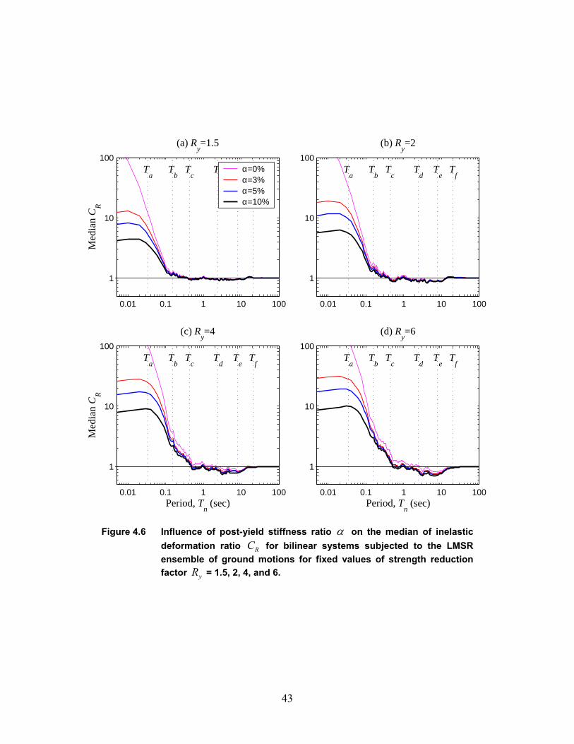
43

0.01 0.1 1 10 100

1

10

100

(a) Ry=1.5

Med

ian

CR

Ta

Tb

Tc

Td

Te

Tf

α=0% α=3% α=5% α=10%

0.01 0.1 1 10 100

1

10

100

(b) Ry=2

Ta

Tb

Tc

Td

Te

Tf

0.01 0.1 1 10 100

1

10

100

(c) Ry=4

Period, Tn (sec)

Med

ian

CR

Ta

Tb

Tc

Td

Te

Tf

0.01 0.1 1 10 100

1

10

100

(d) Ry=6

Period, Tn (sec)

Ta

Tb

Tc

Td

Te

Tf

Figure 4.6 Influence of post-yield stiffness ratio α on the median of inelastic deformation ratio RC for bilinear systems subjected to the LMSR ensemble of ground motions for fixed values of strength reduction factor yR = 1.5, 2, 4, and 6.

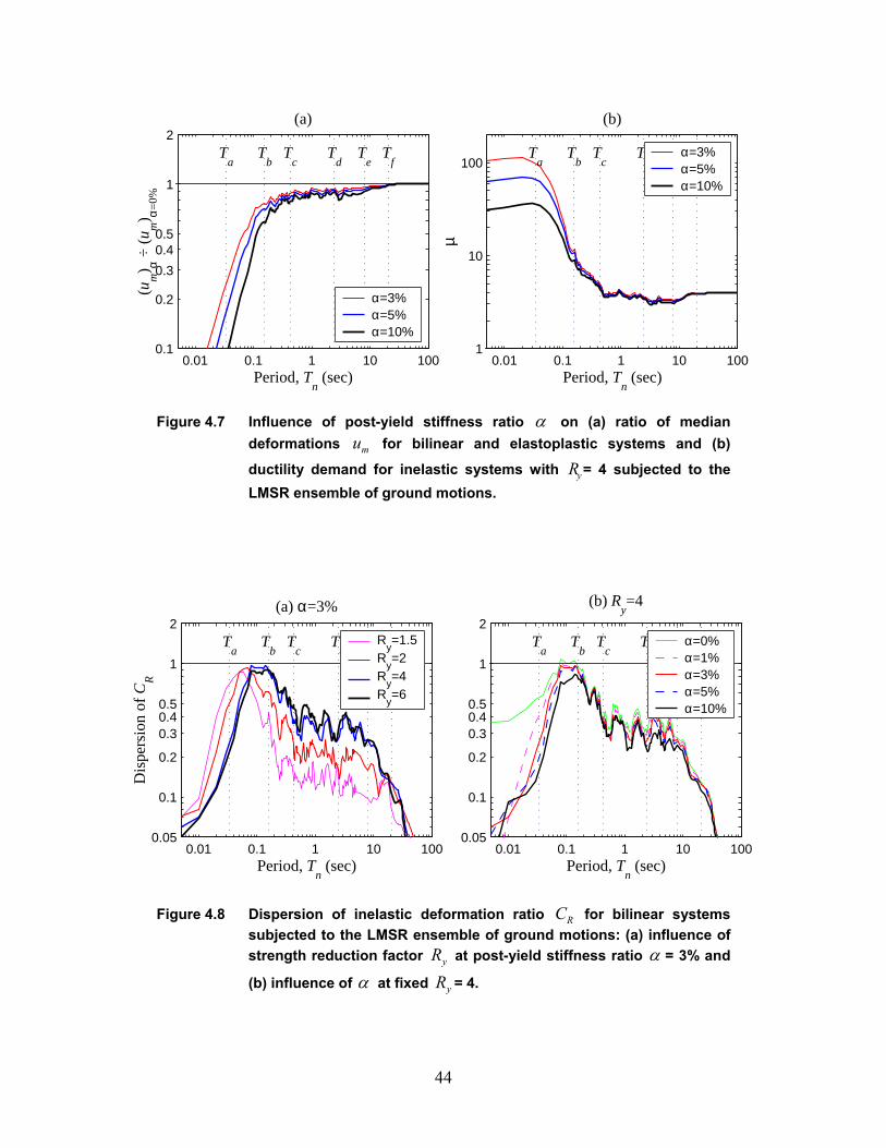
44

0.01 0.1 1 10 1000.1

0.2

0.3

0.40.5

1

2(a)

(um) α ÷

(u m

) α=0%

Period, Tn (sec)

Ta

Tb

Tc

Td

Te

Tf

α=3% α=5% α=10%

0.01 0.1 1 10 1001

10

100

(b)

Period, Tn (sec)

µ

Ta

Tb

Tc

Td

Te

Tf

α=3% α=5% α=10%

Figure 4.7 Influence of post-yield stiffness ratio α on (a) ratio of median deformations mu for bilinear and elastoplastic systems and (b)

ductility demand for inelastic systems with yR = 4 subjected to the LMSR ensemble of ground motions.

0.01 0.1 1 10 1000.05

0.1

0.2

0.30.40.5

1

2

(b) Ry=4

Period, Tn (sec)

Ta

Tb

Tc

Td

Te

Tf

α=0% α=1% α=3% α=5% α=10%

0.01 0.1 1 10 1000.05

0.1

0.2

0.30.40.5

1

2(a) α=3%

Period, Tn (sec)

Dis

pers

ion

of C

R

Ta

Tb

Tc

Td

Te

Tf

Ry=1.5

Ry=2

Ry=4

Ry=6

Figure 4.8 Dispersion of inelastic deformation ratio RC for bilinear systems subjected to the LMSR ensemble of ground motions: (a) influence of strength reduction factor yR at post-yield stiffness ratio α = 3% and

(b) influence of α at fixed yR = 4.

45

5. INFLUENCE OF MAGNITUDE, DISTANCE, SITE CLASS, AND NEAR-FAULT GROUND MOTIONS

5.1 INFLUENCE OF EARTHQUAKE MAGNITUDE AND DISTANCE

The computations that led to the results of the preceding section were repeated for the LMSR,

LMLR, SMSR, and SMLR ground motion ensembles. As observed earlier, the shapes of the four

median response spectra are very similar (Fig. 3.14a) and their cT values—0.43, 0.46, 0.41, and

0.44 sec, respectively—are also close. This similarity suggests that the median Cµ versus nT and

RC versus nT functions should be quite similar. This expectation is confirmed by the

deformation ratio-period plots for the four ensembles shown in Figs. 5.1a and 5.1b.

5.2 INFLUENCE OF FIRM SITE CLASSES

Similar computations were repeated for three ensembles of ground motions recorded on firm

sites: NEHRP site classes B, C, and D. As observed earlier, the shapes of the three median

response spectra are similar (Fig. 3.14b) and their cT values—0.33, 0.33, and 0.41 sec,

respectively—are also similar. Although the cT values for the three site classes vary over a wider

range compared to when earthquake magnitude and recording distance were varied, the median

Cµ versus nT curves (Fig. 5.2a) and RC versus nT curves (Fig. 5.2b) for the three site classes are

very similar; they are close to the LMSR result in spite of the difference in their spectra (Fig.

3.14b).

5.3 NEAR-FAULT GROUND MOTIONS

As mentioned earlier, the median response spectra for the fault-normal and fault-parallel

components of near-fault ground motions display a significantly different shape—with much

different cT =0.85 and 0.61 sec—compared to far-fault ground motions, e.g., the LMSR ensemble

(Fig. 3.14c). Because of these differences, the inelastic deformation ratios Cµ and RC for near-

fault ground motions is significantly different than far-fault motions (Figs. 5.3a and 5.4a), which

is consistent with earlier work reported by Báez and Miranda [2000]. This systematic difference

between the values of RC for near-fault and far-fault ground motions in the acceleration-

46

sensitive spectral region is primarily due to the difference between the period cT values for the

two sets of excitations, as demonstrated by replotting these data against the normalized vibration

period nT / cT in Figs. 5.3b and 5.4b, first introduced by Chopra and Chintanapakdee [2001]. Now

the Cµ values for the far-fault ground motions and both—fault-normal and fault-parallel—

components of near-fault ground motions are close in the acceleration-sensitive ( nT < cT ) region

of the spectrum, and also in the velocity and displacement-sensitive spectral regions, nT > cT (Fig.

5.3b); the same observation applies also to RC (Fig. 5.4b).

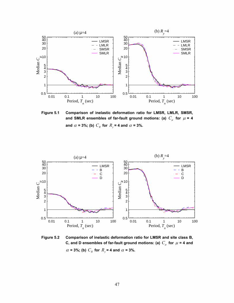
47

0.01 0.1 1 10 1000.5

1

2345

10

20304050

Med

ian

Cµ

(a) µ=4

Period, Tn (sec)

LMSRLMLRSMSRSMLR

0.01 0.1 1 10 1000.5

1

2345

10

20304050

Med

ian

CR

(b) Ry=4

Period, Tn (sec)

LMSRLMLRSMSRSMLR

Figure 5.1 Comparison of inelastic deformation ratio for LMSR, LMLR, SMSR, and SMLR ensembles of far-fault ground motions: (a) Cµ for µ = 4

and α = 3%; (b) RC for yR = 4 and α = 3%.

0.01 0.1 1 10 1000.5

1

2345

10

20304050

Med

ian

Cµ

(a) µ=4

Period, Tn (sec)

LMSRB C D

0.01 0.1 1 10 1000.5

1

2345

10

20304050

Med

ian

CR

(b) Ry=4

Period, Tn (sec)

LMSRB C D

Figure 5.2 Comparison of inelastic deformation ratio for LMSR and site class B, C, and D ensembles of far-fault ground motions: (a) Cµ for µ = 4 and

α = 3%; (b) RC for yR = 4 and α = 3%.

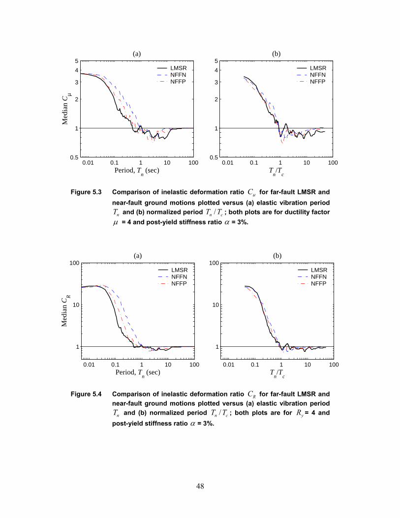
48

0.01 0.1 1 10 1000.5

1

2

3

4

5

Period, Tn (sec)

Med

ian

Cµ

(a)

LMSRNFFNNFFP

0.01 0.1 1 10 1000.5

1

2

3

4

5(b)

Tn/T

c

LMSRNFFNNFFP

Figure 5.3 Comparison of inelastic deformation ratio Cµ for far-fault LMSR and near-fault ground motions plotted versus (a) elastic vibration period

nT and (b) normalized period /n cT T ; both plots are for ductility factor µ = 4 and post-yield stiffness ratio α = 3%.

0.01 0.1 1 10 100

1

10

100

Period, Tn (sec)

Med

ian

CR

(a)

LMSRNFFNNFFP

0.01 0.1 1 10 100

1

10

100(b)

Tn/T

c

LMSRNFFNNFFP

Figure 5.4 Comparison of inelastic deformation ratio RC for far-fault LMSR and near-fault ground motions plotted versus (a) elastic vibration period

nT and (b) normalized period /n cT T ; both plots are for yR = 4 and post-yield stiffness ratio α = 3%.

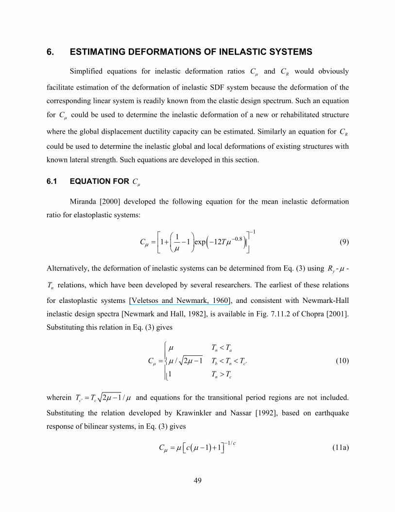
49

6. ESTIMATING DEFORMATIONS OF INELASTIC SYSTEMS

Simplified equations for inelastic deformation ratios Cµ and RC would obviously

facilitate estimation of the deformation of inelastic SDF system because the deformation of the

corresponding linear system is readily known from the elastic design spectrum. Such an equation

for Cµ could be used to determine the inelastic deformation of a new or rehabilitated structure

where the global displacement ductility capacity can be estimated. Similarly an equation for RC

could be used to determine the inelastic global and local deformations of existing structures with

known lateral strength. Such equations are developed in this section.

6.1 EQUATION FOR Cµ

Miranda [2000] developed the following equation for the mean inelastic deformation

ratio for elastoplastic systems:

( )1

0.811 1 exp 12C Tµ µµ

−−

= + − −

(9)

Alternatively, the deformation of inelastic systems can be determined from Eq. (3) using yR - µ -

nT relations, which have been developed by several researchers. The earliest of these relations

for elastoplastic systems [Veletsos and Newmark, 1960], and consistent with Newmark-Hall

inelastic design spectra [Newmark and Hall, 1982], is available in Fig. 7.11.2 of Chopra [2001].

Substituting this relation in Eq. (3) gives

'/ 2 1

1

n a

b n c

n c

T T

C T T T

T Tµ

µ

µ µ

<= − < < >

(10)

wherein ' 2 1 /c cT T µ µ= − and equations for the transitional period regions are not included.

Substituting the relation developed by Krawinkler and Nassar [1992], based on earthquake

response of bilinear systems, in Eq. (3) gives

( ) 1/1 1 cC cµ µ µ−

= − + (11a)

https://www.researchgate.net/publication/246019619_Effect_of_Inelastic_Behaviour_on_the_Response_of_Simple_Systems_to_Earthquake_Motions?el=1_x_8&enrichId=rgreq-91e216be17565a0c177518e7541077f3-XXX&enrichSource=Y292ZXJQYWdlOzI0NTMwNDg4MDtBUzoxMjkzMTA5NzUzMzY0NDhAMTQwNzg0MTU0NzI0Mw==

50

where

( , )1

an

n ann

T bc TTT

α = ++

(11b)

and the numerical coefficients depend on the post-yield stiffness ratio, α : 1a = and 0.42b = for

0α = ; 1a = and 0.37b = for 2%α = ; 0.8a = and 0.29b = for 10%α = .

Figure 6.1a compares Eqs. (9), (10), and (11) for α = 0 with the mean value of Cµ

determined earlier (Fig. 4.1) for elastoplastic systems subjected to the LMSR ensemble of

ground motions. Only results for ductility factor of 6 (the largest value considered) are presented

because it is the severest test of the Cµ -equations. Even for this extreme case, Eqs. (9), (10), and

(11) provide excellent estimates of the inelastic deformation for elastoplastic systems,

irrespective of the fact that they were developed for ground motion ensembles different than the

LMSR ensemble; the latter two equations are based on an indirect method, with the bias

identified by Miranda [2001]. A similar comparison for α =10% (Fig. 6.1b) demonstrates that

Eq. (11) (specialized for 10%α = ) is satisfactory over a wide range of periods but overestimates

Cµ at very short periods because as nT tends to zero, Eq. (11) approaches µ —a limiting value

that is valid only for elastoplastic systems—instead of Eq. (7a) derived earlier. Because Eqs. (9)

and (10) were developed from response data for elastoplastic systems, as expected they

overestimate Cµ for bilinear systems; note that Eq. (9) is based on mean value of Cµ , which is

larger than the median value for probability density functions that are skewed to the right.

Presented next is an improved equation that fits the median Cµ data for any ensemble of

ground motions, but ignores the data showing Cµ <1 over the period range dT to fT (Fig. 4.1a)

and satisfies the limiting values of Cµ at nT = 0 and nT = ∞ [Eqs. (7a) and (8)]. Such a function

for Cµ has been derived [Appendix A] in terms of ductility factor µ and the normalized period

nT / cT :

( )1

11 1

d

nb

c

TaC L cTµ µ µ

−

− = + − + +

(12)

51

where Lµ is given by Eq. (7a). The numerical parameters a, b, c, and d were determined from the

response data by the algorithm (fmins.m) in MATLAB to minimize the residual error, defined as

the sum of the squares of differences between the actual data and the regression equation, but

with a penalty for underestimation: a = 72, b = 2.2, c = 1.6, and d = 1.5 using the LMSR data

and a = 105, b = 2.3, c = 1.9, d = 1.7 using the data for four (LMSR, LMLR, SMSR, and SMLR)

ensembles; these parameter values are independent of post-yield stiffness ratio, α .

Figure 6.2 shows that Eq. (12) with the first set of parameter values and 0.43cT = sec

closely matches the median Cµ computed for the LMSR and near-fault ground motions. The

excellent agreement with the LMSR data is expected because the parameters were determined

from those data. Most impressive is that the same parameters provide a good match with the

near-fault data, which has been achieved because Eq. (12) is developed as a function of /n cT T ,

the normalized period, instead of nT .

Figures 6.3 to 6.7 show that Eq. (12), which uses the second set of values for a, b, c, and

d, provides a satisfactory fit to the median Cµ computed for LMSR, LMLR, SMSR, and SMLR

ground motion ensembles (Fig. 6.3); NEHRP site class B, C, and D ensembles (Fig. 6.4); near-

fault NF-FN and NF-FP ensembles (Fig. 6.5); near-fault NF-FN (soil33) and NF-FP (soil33)

ensembles (Fig. 6.6); and near-fault NF-FN (rock12) and NF-FP (rock12) ensembles (Fig. 6.7).

Thus, these parameter values are generally applicable for a wide range of conditions, except for

soft soil sites, and even for a large ensemble of near-fault ground motions. A more complicated

equation would be necessary to match the Cµ < 1 data in the dT -to- fT period range; however,

these data should be re-examined with P- ∆ effects included before developing such an equation.

6.2 EQUATION FOR RC

Ruiz-Garcia and Miranda [2002] developed the following equation for the mean inelastic

deformation ratio for elastoplastic systems

( )

( )1 11 1/

R bs

C Rca T T

= + + −

(13)

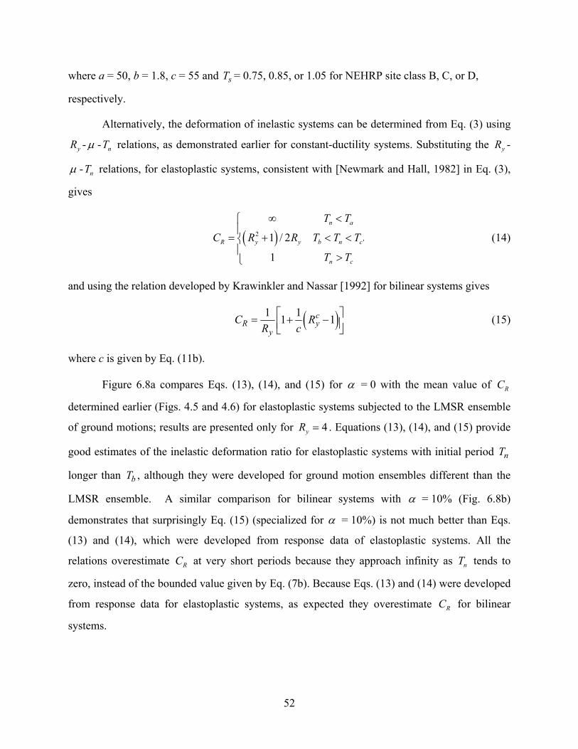
52

where a = 50, b = 1.8, c = 55 and sT = 0.75, 0.85, or 1.05 for NEHRP site class B, C, or D,

respectively.

Alternatively, the deformation of inelastic systems can be determined from Eq. (3) using

yR - µ - nT relations, as demonstrated earlier for constant-ductility systems. Substituting the yR -

µ - nT relations, for elastoplastic systems, consistent with [Newmark and Hall, 1982] in Eq. (3),

gives

( )2'1 / 2

1

n a

R y y b n c

n c

T T

C R R T T T

T T

∞ <

= + < < >

(14)

and using the relation developed by Krawinkler and Nassar [1992] for bilinear systems gives

( )1 11 1cR y

yC R

R c = + −

(15)

where c is given by Eq. (11b).

Figure 6.8a compares Eqs. (13), (14), and (15) for α = 0 with the mean value of RC

determined earlier (Figs. 4.5 and 4.6) for elastoplastic systems subjected to the LMSR ensemble

of ground motions; results are presented only for 4yR = . Equations (13), (14), and (15) provide

good estimates of the inelastic deformation ratio for elastoplastic systems with initial period nT

longer than bT , although they were developed for ground motion ensembles different than the

LMSR ensemble. A similar comparison for bilinear systems with α = 10% (Fig. 6.8b)

demonstrates that surprisingly Eq. (15) (specialized for α = 10%) is not much better than Eqs.

(13) and (14), which were developed from response data of elastoplastic systems. All the

relations overestimate RC at very short periods because they approach infinity as nT tends to

zero, instead of the bounded value given by Eq. (7b). Because Eqs. (13) and (14) were developed

from response data for elastoplastic systems, as expected they overestimate RC for bilinear

systems.

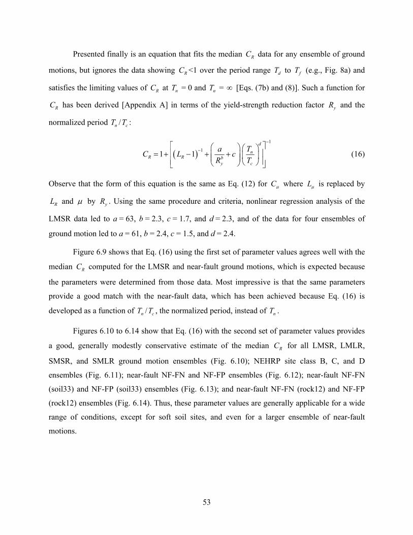
53

Presented finally is an equation that fits the median RC data for any ensemble of ground

motions, but ignores the data showing RC <1 over the period range dT to fT (e.g., Fig. 8a) and

satisfies the limiting values of RC at nT = 0 and nT = ∞ [Eqs. (7b) and (8)]. Such a function for

RC has been derived [Appendix A] in terms of the yield-strength reduction factor yR and the

normalized period nT / cT :

( )1

11 1d

nR R b

y c

TaC L cR T

−

− = + − + +

(16)

Observe that the form of this equation is the same as Eq. (12) for Cµ where Lµ is replaced by

RL and µ by yR . Using the same procedure and criteria, nonlinear regression analysis of the

LMSR data led to a = 63, b = 2.3, c = 1.7, and d = 2.3, and of the data for four ensembles of

ground motion led to a = 61, b = 2.4, c = 1.5, and d = 2.4.

Figure 6.9 shows that Eq. (16) using the first set of parameter values agrees well with the

median RC computed for the LMSR and near-fault ground motions, which is expected because

the parameters were determined from those data. Most impressive is that the same parameters

provide a good match with the near-fault data, which has been achieved because Eq. (16) is

developed as a function of nT / cT , the normalized period, instead of nT .

Figures 6.10 to 6.14 show that Eq. (16) with the second set of parameter values provides

a good, generally modestly conservative estimate of the median RC for all LMSR, LMLR,

SMSR, and SMLR ground motion ensembles (Fig. 6.10); NEHRP site class B, C, and D

ensembles (Fig. 6.11); near-fault NF-FN and NF-FP ensembles (Fig. 6.12); near-fault NF-FN

(soil33) and NF-FP (soil33) ensembles (Fig. 6.13); and near-fault NF-FN (rock12) and NF-FP

(rock12) ensembles (Fig. 6.14). Thus, these parameter values are generally applicable for a wide

range of conditions, except for soft soil sites, and even for a larger ensemble of near-fault

motions.

54

0.01 0.1 1 10 1000.5

1

2

3

5

10(a) α=0%

Period, Tn (sec)

Cµ

LMSR Data Miranda Newmark−Hall Krawinkler−Nassar

0.01 0.1 1 10 1000.5

1

2

3

5

10(b) α=10%

Period, Tn (sec)

Figure 6.1 Comparison of mean inelastic deformation ratio Cµ estimated by equations developed by various researchers and LMSR data for ductility factor µ = 6: (a) elastoplastic systems, and (b) post-yield stiffness systems (α =10%).

55

0.01 0.1 1 10 1000.5

1

2

3

45

10(a) α=0%, µ=2

Cµ

LMSR NFFN Proposed Cµ

0.01 0.1 1 10 1000.5

1

2

3

45

10(c) α=0%, µ=6

Tn/T

c

Cµ

0.01 0.1 1 10 1000.5

1

2

3

45

10(b) α=10%, µ=2

0.01 0.1 1 10 1000.5

1

2

3

45

10(d) α=10%, µ=6

Tn/T

c

Figure 6.2 Comparison of median inelastic deformation ratio Cµ estimated by proposed equation with computed data for LMSR-far-fault and near-fault (fault-normal component) ground motions for elastoplastic ( 0α = ) and bilinear ( 10%α = ) systems; and µ = 2 and 6.

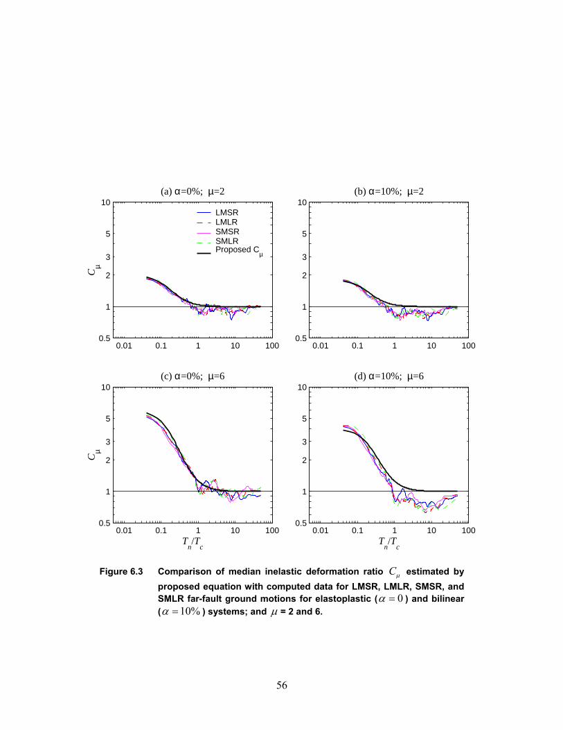
56

0.01 0.1 1 10 1000.5

1

2

3

5

10(a) α=0%; µ=2

Cµ

LMSR LMLR SMSR SMLR Proposed Cµ

0.01 0.1 1 10 1000.5

1

2

3

5

10(c) α=0%; µ=6

Cµ

Tn/T

c

0.01 0.1 1 10 1000.5

1

2

3

5

10(b) α=10%; µ=2

0.01 0.1 1 10 1000.5

1

2

3

5

10(d) α=10%; µ=6

Tn/T

c

Figure 6.3 Comparison of median inelastic deformation ratio Cµ estimated by proposed equation with computed data for LMSR, LMLR, SMSR, and SMLR far-fault ground motions for elastoplastic ( 0α = ) and bilinear ( 10%α = ) systems; and µ = 2 and 6.

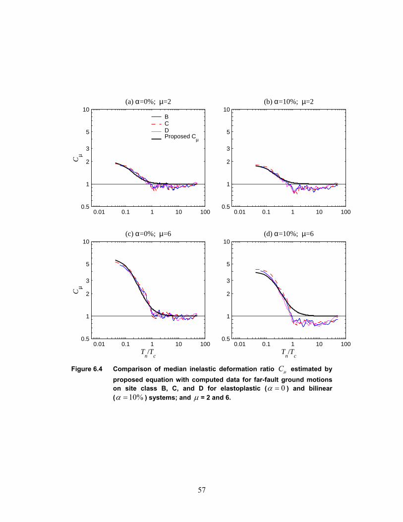
57

0.01 0.1 1 10 1000.5

1

2

3

5

10(a) α=0%; µ=2

Cµ

B C D Proposed Cµ

0.01 0.1 1 10 1000.5

1

2

3

5

10(c) α=0%; µ=6

Cµ

Tn/T

c

0.01 0.1 1 10 1000.5

1

2

3

5

10(b) α=10%; µ=2

0.01 0.1 1 10 1000.5

1

2

3

5

10(d) α=10%; µ=6

Tn/T

c

Figure 6.4 Comparison of median inelastic deformation ratio Cµ estimated by proposed equation with computed data for far-fault ground motions on site class B, C, and D for elastoplastic ( 0α = ) and bilinear ( 10%α = ) systems; and µ = 2 and 6.

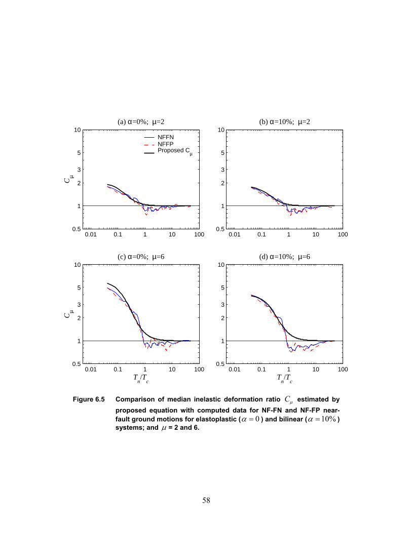
58

0.01 0.1 1 10 1000.5

1

2

3

5

10(a) α=0%; µ=2

Cµ

NFFN NFFP Proposed Cµ

0.01 0.1 1 10 1000.5

1

2

3

5

10(c) α=0%; µ=6

Cµ

Tn/T

c

0.01 0.1 1 10 1000.5

1

2

3

5

10(b) α=10%; µ=2

0.01 0.1 1 10 1000.5

1

2

3

5

10(d) α=10%; µ=6

Tn/T

c

Figure 6.5 Comparison of median inelastic deformation ratio Cµ estimated by proposed equation with computed data for NF-FN and NF-FP near-fault ground motions for elastoplastic ( 0α = ) and bilinear ( 10%α = ) systems; and µ = 2 and 6.

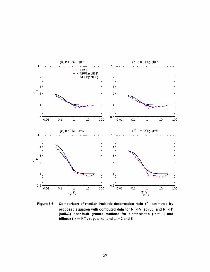
59

0.01 0.1 1 10 1000.5

1

2

3

5

10(a) α=0%; µ=2

Cµ


0.01 0.1 1 10 1000.5

1

2

3

5

10(c) α=0%; µ=6

Cµ

Tn/T

c

0.01 0.1 1 10 1000.5

1

2

3

5

10(b) α=10%; µ=2

0.01 0.1 1 10 1000.5

1

2

3

5

10(d) α=10%; µ=6

Tn/T

c

Figure 6.6 Comparison of median inelastic deformation ratio Cµ estimated by proposed equation with computed data for NF-FN (soil33) and NF-FP (soil33) near-fault ground motions for elastoplastic ( 0α = ) and bilinear ( 10%α = ) systems; and µ = 2 and 6.

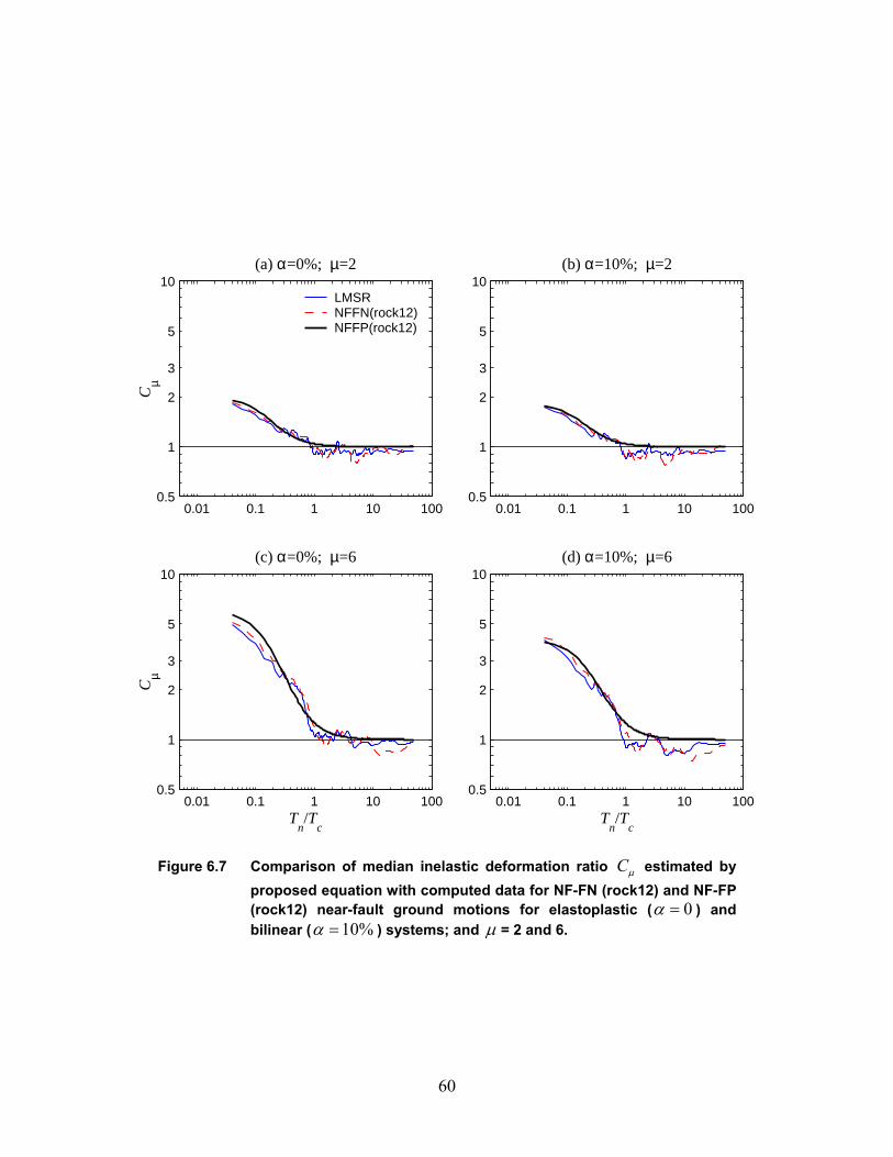
60

0.01 0.1 1 10 1000.5

1

2

3

5

10(a) α=0%; µ=2

Cµ


0.01 0.1 1 10 1000.5

1

2

3

5

10(c) α=0%; µ=6

Cµ

Tn/T

c

0.01 0.1 1 10 1000.5

1

2

3

5

10(b) α=10%; µ=2

0.01 0.1 1 10 1000.5

1

2

3

5

10(d) α=10%; µ=6

Tn/T

c

Figure 6.7 Comparison of median inelastic deformation ratio Cµ estimated by proposed equation with computed data for NF-FN (rock12) and NF-FP (rock12) near-fault ground motions for elastoplastic ( 0α = ) and bilinear ( 10%α = ) systems; and µ = 2 and 6.

61

0.01 0.1 1 10 100

1

10

100(a) α=0%

Period, Tn (sec)

CR

LMSR Data Ruiz Garcia−MirandaNewmark−Hall Krawinkler−Nassar

0.01 0.1 1 10 100

1

10

100(b) α=10%

Period, Tn (sec)

Figure 6.8 Comparison of mean inelastic deformation ratio RC estimated by equations developed by various researchers and LMSR data for yR = 4: (a) elastoplastic systems, and (b) bilinear systems (α =10%).

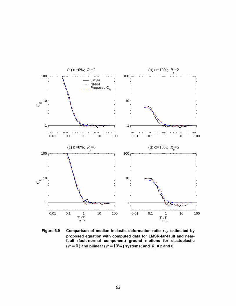
62

0.01 0.1 1 10 100

1

10

100

(a) α=0%; Ry=2

CR

LMSR NFFN Proposed C

R

0.01 0.1 1 10 100

1

10

100

(c) α=0%; Ry=6

CR

Tn/T

c

0.01 0.1 1 10 100

1

10

100

(b) α=10%; Ry=2

0.01 0.1 1 10 100

1

10

100

(d) α=10%; Ry=6

Tn/T

c

Figure 6.9 Comparison of median inelastic deformation ratio RC estimated by proposed equation with computed data for LMSR-far-fault and near-fault (fault-normal component) ground motions for elastoplastic ( 0α = ) and bilinear ( 10%α = ) systems; and yR = 2 and 6.

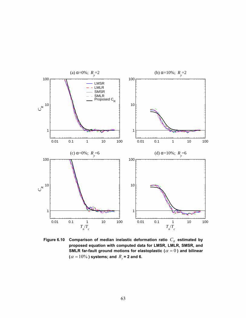
63

0.01 0.1 1 10 100

1

10

100

(a) α=0%; Ry=2

CR

LMSR LMLR SMSR SMLR Proposed C

R

0.01 0.1 1 10 100

1

10

100

(c) α=0%; Ry=6

CR

Tn/T

c

0.01 0.1 1 10 100

1

10

100

(b) α=10%; Ry=2

0.01 0.1 1 10 100

1

10

100

(d) α=10%; Ry=6

Tn/T

c

Figure 6.10 Comparison of median inelastic deformation ratio RC estimated by proposed equation with computed data for LMSR, LMLR, SMSR, and SMLR far-fault ground motions for elastoplastic ( 0α = ) and bilinear ( 10%α = ) systems; and yR = 2 and 6.

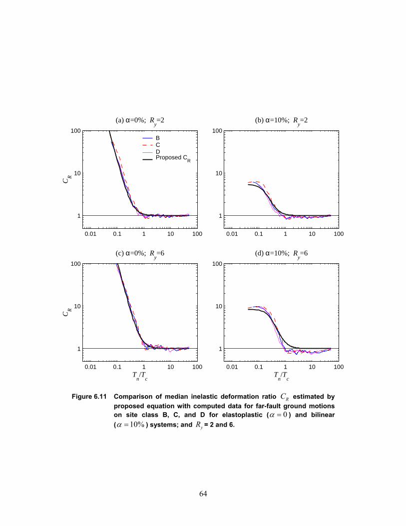
64

0.01 0.1 1 10 100

1

10

100

(a) α=0%; Ry=2

CR

B C D Proposed C

R

0.01 0.1 1 10 100

1

10

100

(c) α=0%; Ry=6

CR

Tn/T

c

0.01 0.1 1 10 100

1

10

100

(b) α=10%; Ry=2

0.01 0.1 1 10 100

1

10

100

(d) α=10%; Ry=6

Tn/T

c

Figure 6.11 Comparison of median inelastic deformation ratio RC estimated by proposed equation with computed data for far-fault ground motions on site class B, C, and D for elastoplastic ( 0α = ) and bilinear ( 10%α = ) systems; and yR = 2 and 6.

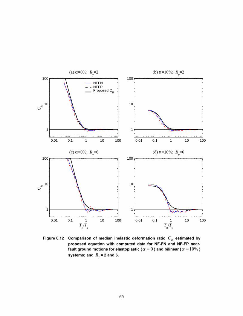
65

0.01 0.1 1 10 100

1

10

100

(a) α=0%; Ry=2

CR

NFFN NFFP Proposed C

R

0.01 0.1 1 10 100

1

10

100

(c) α=0%; Ry=6

CR

Tn/T

c

0.01 0.1 1 10 100

1

10

100

(b) α=10%; Ry=2

0.01 0.1 1 10 100

1

10

100

(d) α=10%; Ry=6

Tn/T

c

Figure 6.12 Comparison of median inelastic deformation ratio RC estimated by proposed equation with computed data for NF-FN and NF-FP near-fault ground motions for elastoplastic ( 0α = ) and bilinear ( 10%α = ) systems; and yR = 2 and 6.

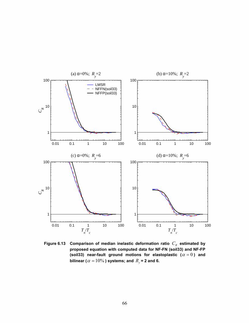
66

0.01 0.1 1 10 100

1

10

100

(a) α=0%; Ry=2

CR


0.01 0.1 1 10 100

1

10

100

(c) α=0%; Ry=6

CR

Tn/T

c

0.01 0.1 1 10 100

1

10

100

(b) α=10%; Ry=2

0.01 0.1 1 10 100

1

10

100

(d) α=10%; Ry=6

Tn/T

c

Figure 6.13 Comparison of median inelastic deformation ratio RC estimated by proposed equation with computed data for NF-FN (soil33) and NF-FP (soil33) near-fault ground motions for elastoplastic ( 0α = ) and bilinear ( 10%α = ) systems; and yR = 2 and 6.

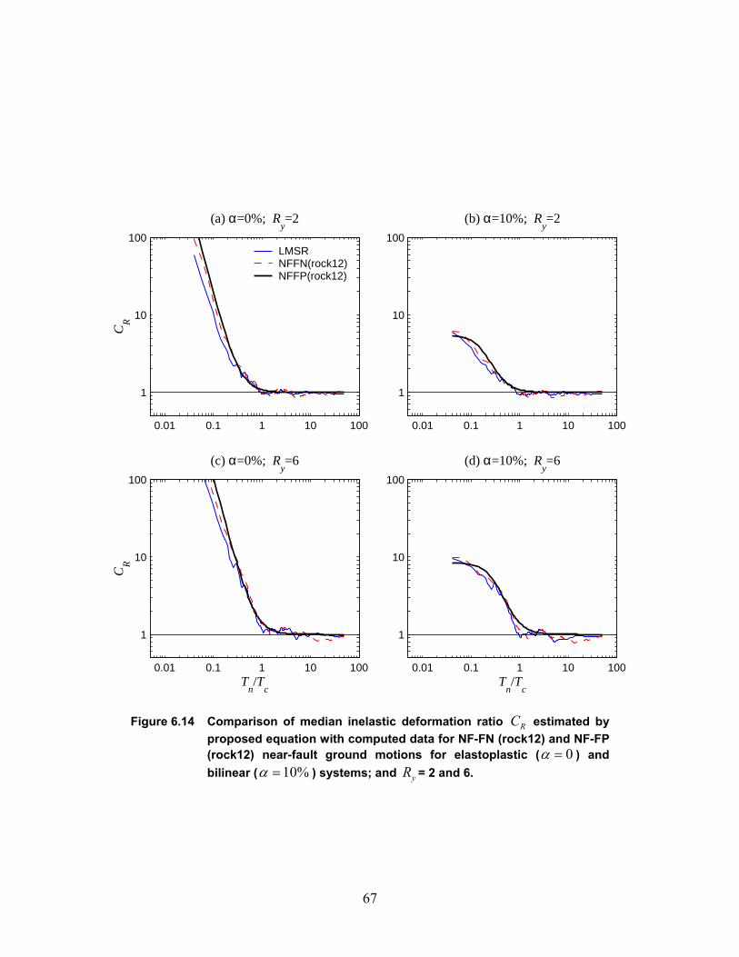
67

0.01 0.1 1 10 100

1

10

100

(a) α=0%; Ry=2

CR


0.01 0.1 1 10 100

1

10

100

(c) α=0%; Ry=6

CR

Tn/T

c

0.01 0.1 1 10 100

1

10

100

(b) α=10%; Ry=2

0.01 0.1 1 10 100

1

10

100

(d) α=10%; Ry=6

Tn/T

c

Figure 6.14 Comparison of median inelastic deformation ratio RC estimated by proposed equation with computed data for NF-FN (rock12) and NF-FP (rock12) near-fault ground motions for elastoplastic ( 0α = ) and bilinear ( 10%α = ) systems; and yR = 2 and 6.

69

7. CONCLUSIONS

This investigation of the median and dispersion of the ratio of deformations—denoted by

Cµ for system with known ductility factor µ and by RC for systems with known yield strength

reduction factor yR —of bilinearly inelastic and corresponding linear systems over eight

ensembles of ground motions, has led to the following conclusions:

1. Equations have been derived for Lµ and RL , the limiting values of Cµ and RC as the

elastic vibration period nT of the system tends to zero. Lµ depends on µ and α , the

post-yield stiffness ratio; RL depends on yR and α . For the special case of elastoplastic

systems, Lµ µ= and RL = ∞ . Post-yield stiffness is much more influential in reducing

RL —from an unbounded value to a finite value—than Lµ . For the limiting case of

nT = ∞ , physical reasoning leads to 1RC Cµ = = , the well-known equal deformation rule

[Veletsos and Newmark, 1960].

2. The median values of Cµ (and RC ) for the seven ensembles of far-fault ground motions

confirm known results that Cµ (and RC ) exceed 1 in the acceleration-sensitive spectral

region, increasing with µ (and yR ); ≈1 in the velocity-sensitive and displacement-

sensitive regions, essentially independent of µ (and yR ); except that they fall below 1 in

the period range dT to fT of the latter region, decreasing for increasing µ (and yR ). For

very short-period systems ( n aT T< ), RC is very sensitive to the yield strength and can be

very large even if the strength of the system is only slightly smaller than that required for

it to remain elastic.

3. In contrast to the prevailing view, based largely on earthquake response of SDF systems

for fixed ductility factor, ignoring post-yield stiffness in estimating deformation is too

conservative for seismic evaluation of existing structures with known yR in the

acceleration-sensitive region.

70

4. The dispersion of Cµ is zero as nT tends to zero or infinity; roughly similar over a wide

period range, bT to fT ; increasing with µ ; and affected little by post-yield stiffness.

5. The dispersion of RC is zero as nT tends to zero (except for elastoplastic systems) or nT

tends to infinity is larger for weaker systems over a wide range of periods except for

n bT T< where this trend is reversed; and is essentially independent of post-yield stiffness

ratio for the range of α considered in the velocity- and displacement-sensitive regions,

but is reduced significantly with the slightest post-yield stiffness in the short-period

portion of the acceleration-sensitive region.

6. The median Cµ versus nT plots for four ground motion ensembles denoted by LMSR,

LMLR, SMSR, and SMLR—representing four combinations of large (M = 6.6-6.9) or

small (M = 5.8-6.5) magnitude and small (R = 13-30 km) or large (R = 30-60 km)

distance—are very similar; the RC - nT plots of the four ensembles are also very close.

7. The median Cµ - nT and RC - nT plots are essentially independent of NEHRP site classes

B, C, and D, all of which are firm soil sites.

8. In the acceleration-sensitive spectral region, the median Cµ - nT and RC - nT plots for

near-fault ground motions are systematically different than far-fault ground motions;

however, when plotted against normalized period /n cT T (where cT is the period

separating the acceleration- and velocity-sensitive regions), they become very similar in

all spectral regions.

9. Simplified equations for inelastic deformation ratios of Cµ [Eq. (12)] and RC [Eq. (16)]

for elastoplastic and bilinear systems have been developed as functions of /n cT T , and µ

or yR , respectively. These equations satisfy the limiting values: Lµ and RL at nT = 0,

and 1 at nT = ∞ . Determined by regression analysis of the Cµ and RC data for four

ensembles (LMSR, LMLR, SMSR, and SMLR) of far-fault ground motions, the

numerical values for the parameters in these equations are as follows: a = 105, b = 2.3, c

= 1.9, and d = 1.7 in Eq. (12); and a = 61, b = 2.4, c = 1.5, and d = 2.4 in Eq. (16). These

71

equations and parameters are also valid for near-fault ground motions recorded on rock

and soil and far-fault ground motions recorded on NEHRP site classes B, C, and D. Thus

the equations presented for Cµ and RC should be valid for almost any ensemble of

ground motions recorded at firm sites. The equation for Cµ should be useful in

estimating the inelastic deformation of a new or rehabilitated structure where the global

ductility capacity can be estimated. Similarly, the equation for RC should be useful for

existing structures with known lateral strength.

73

8. REFERENCES

Applied Technology Council (1996). “Seismic evaluation and retrofit of concrete buildings,”

Report No. ATC-40, Redwood City, Calif.

Báez, J. I., and Miranda, E. (2000). “Amplification factors to estimate inelastic displacement

demands for the design of structures in the near field,” CD-Rom Proc., 12th World Conf.

on Earthq. Engrg., Paper No. 1561, Auckland, New Zealand.

Chopra, A. K., and Goel, R. K. (1999). “Capacity-demand-diagram methods based on inelastic

design spectrum,” Earthq. Spectra, 15(4):637-656.

Chopra, A. K. (2001). Dynamics of Structures: Theory and Applications to Earthquake

Engineering, 2nd Ed., Prentice Hall, Englewood Cliffs, New Jersey, 844 pg.

Chopra, A. K., and Chintanapakdee, C. (2001). “Comparing response of SDF systems to near-

fault and far-fault earthquake motions in the context of spectral regions,” Earthq. Engrg.

Struc. Dyn., 30(12):1769-1789.

Chopra, A. K., and Goel, R. K. (2002). “A modal pushover analysis procedure for estimating

seismic demands for buildings,” Earthq. Engrg. Struc. Dyn., 31(3):561-582.

Chopra, A. K., Goel, R. K., and Chintanapakdee, C. (2003), “Statistics of single-degree-of-

freedom estimate of displacement for pushover analysis of buildings,” J. Struc. Engrg.,

ASCE, 119(4)459-469.

Clough, R. W. (1966). “Effect of stiffness degradation on earthquake ductility requirements,”

Rept. No. SEMM 66-16, Dept. of Civil Engrg., Univ. of Calif., Berkeley, Calif., 67 pg.

Fajfar, P. (2000). “A nonlinear analysis method for performance-based seismic design,” Earthq.

Spectra, 16(3):573-592.

Federal Emergency Management Agency (1997). ‘‘NEHRP guidelines for the seismic

rehabilitation of buildings,’’ Rept. FEMA 273 (Guidelines) and Rept. 274 (Commentary),

Washington, D.C.

Federal Emergency Management Agency (2000). ‘‘Prestandard and commentary for the seismic

rehabilitation of buildings,’’ Rept. FEMA 356, Washington, D.C.

Gupta, A., and Krawinkler, H. (1998). “Effect of stiffness degradation on deformation demands

for SDOF and MDOF structures,” Proc., 6th Nat. Conf. Earthq. Engrg., Earthq. Engrg.

Res. Inst., Oakland, Calif.







https://www.researchgate.net/publication/247646818_Statistics_of_Single-Degree-of-Freedom_Estimate_of_Displacement_for_Pushover_Analysis_of_Buildings?el=1_x_8&enrichId=rgreq-91e216be17565a0c177518e7541077f3-XXX&enrichSource=Y292ZXJQYWdlOzI0NTMwNDg4MDtBUzoxMjkzMTA5NzUzMzY0NDhAMTQwNzg0MTU0NzI0Mw==



74

Gupta, B., and Kunnath, S. (1998). “Effect of hysteretic model parameters on inelastic seismic

demands,” Proc., 6th Nat. Conf. Earthq. Engrg., Earthq. Engrg. Res. Inst., Oakland, Calif.

Krawinkler, H., and Nassar, A. A. (1992). “Seismic design based on ductility and cumulative

damage demands and capacities,” In: Nonlinear Seismic Analysis and Design of

Reinforced Concrete Buildings, Eds. P. Fajfar and H. Krawinkler. New York: Elsevier

Applied Science.

MATLAB: The Language of Technical Computing (1997). Version 5.0, The Mathworks Inc.,

Natick, Mass.

Miranda, E. (1991). “Seismic evaluation and upgrading of existing structures,” Ph.D. thesis,

Dept. of Civil Engrg., Univ. of Calif., Berkeley, Berkeley, Calif.

Miranda, E. (1993). “Evaluation of site-dependent inelastic seismic design spectra,” J. Struct.

Engrg., ASCE, 119(5):1319–1338.

Miranda, E. (2000). “Inelastic displacement ratios for structures on firm sites,” J. Struct. Engrg.,

ASCE, 126(10):1150–1159.

Miranda, E. (2001). “Estimation of inelastic deformation demands of SDOF systems,” J. Struct.

Engrg., ASCE, 127(9):1005-1012.

Nassar, A. A., and Krawinkler, H. (1991). “Seismic demands for SDOF and MDOF systems,”

Rept. No. 95, John A. Blume Earthquake Engrg. Cen., Stanford Univ., Stanford, Calif.,

204 pg.

Newmark, N. M., and Hall, W. J. (1982). Earthquake Spectra and Design, Earthquake

Engineering Research Institute, Berkeley, Calif., 103 pg.

Qi, X., and Moehle, J. P. (1991). “Displacement design approach for reinforced concrete

structures subjected to earthquakes,” Rept. No. EERC-91/02, Earthq. Engrg. Res. Cen.,

Univ. of Calif., Berkeley, Calif.

Riddell, R., and Newmark, N. M. (1979). “Statistical analysis of the response of nonlinear

systems subjected to earthquakes,” Struc. Res. Series No. 468, Dept. of Civil Engrg.,

Univ. of Illinois, Urbana, Ill., 291 pg.

Riddell, R., Garcia, J. E., and Garces, E. (2002). “Inelastic deformation response of SDOF

systems subjected to earthquakes,” Earthq. Engrg. Struc. Dyn., 31(3):515-538.

Ruiz-Garcia, J., and Miranda, E. (2002). “Inelastic displacement ratios for evaluation of existing

structures,” Earthq. Engrg. Struc. Dyn., 32(8):1237-1258.













https://www.researchgate.net/publication/229883192_Inelastic_displacement_ratios_for_evaluation_of_existing_structures?el=1_x_8&enrichId=rgreq-91e216be17565a0c177518e7541077f3-XXX&enrichSource=Y292ZXJQYWdlOzI0NTMwNDg4MDtBUzoxMjkzMTA5NzUzMzY0NDhAMTQwNzg0MTU0NzI0Mw==

https://www.researchgate.net/publication/229883192_Inelastic_displacement_ratios_for_evaluation_of_existing_structures?el=1_x_8&enrichId=rgreq-91e216be17565a0c177518e7541077f3-XXX&enrichSource=Y292ZXJQYWdlOzI0NTMwNDg4MDtBUzoxMjkzMTA5NzUzMzY0NDhAMTQwNzg0MTU0NzI0Mw==





75

Shimazaki, K., and Sozen, M. A. (1984). “Seismic drift of reinforced concrete structures,” Tech.

Res. Rep. of Hazama-Gumi Ltd., Tokyo, pp. 145–166.

Somerville, P. G. (1998). “Development of an improved representation of near-fault ground

motions,” Proc., SMIP98 Seminar on Utilization of Strong-Motion Data, Calif. Div.

Mines and Geology, pp. 1-20. Oakland, Calif.

Song, J. K., and Pincheira, J. A. (2000). “Spectral displacement demands of stiffness- and

strength-degrading systems,” Earthq. Spectra, 16(4):817-851.

Veletsos, A. S., and Newmark, N. M. (1960). “Effect of inelastic behavior on the response of

simple systems to earthquake motions,” Proc., 2nd World Conf. on Earthq. Engrg., 2:895–

912, Tokyo, Japan.

Veletsos, A. S., and Newmark, N. M. (1964). “Response spectra for single-degree-of-freedom

elastic and inelastic systems,” Rept. No. RTD-TDR-63-3096, Vol. III, Air Force Weapons

Lab., Albuquerque, N. Mexico.

Veletsos, A. S., Newmark, N. M., and Chepalati, C. V. (1965). “Deformation spectra for elastic

and elastoplastic systems subjected to ground shock and earthquake motion,” Proc., 3rd

World Conf. on Earthq. Engrg., 2:663–682, Wellington, New Zealand.

Veletsos, A. S. (1969). “Maximum deformations of certain nonlinear systems,” Proc., 4th World

Conf. on Earthq. Engrg., Chilean Assoc. on Seism. and Earthq. Engrg., 2:A4-155 - A4-

170, Santiago, Chile.

Veletsos, A. S., and Vann, W. P. (1971). “Response of ground-excited elastoplastic systems,” J.

Struc. Div., ASCE, 97, ST4:1257-1281.

Whittaker, A., Constantinou, M., and Tsopelas, P. (1998). “Displacement estimates for

performance-based seismic design,” J. Struct. Engrg., ASCE, 124(8):905–912.

https://www.researchgate.net/publication/245303586_Displacement_Estimates_for_Performance-Based_Seismic_Design?el=1_x_8&enrichId=rgreq-91e216be17565a0c177518e7541077f3-XXX&enrichSource=Y292ZXJQYWdlOzI0NTMwNDg4MDtBUzoxMjkzMTA5NzUzMzY0NDhAMTQwNzg0MTU0NzI0Mw==

https://www.researchgate.net/publication/245303586_Displacement_Estimates_for_Performance-Based_Seismic_Design?el=1_x_8&enrichId=rgreq-91e216be17565a0c177518e7541077f3-XXX&enrichSource=Y292ZXJQYWdlOzI0NTMwNDg4MDtBUzoxMjkzMTA5NzUzMzY0NDhAMTQwNzg0MTU0NzI0Mw==






https://www.researchgate.net/publication/245855821_Deformation_Spectra_for_Elastic_and_ElastoPlastic_Systems_Subjected_to_Ground_Shock_and_Earthquake?el=1_x_8&enrichId=rgreq-91e216be17565a0c177518e7541077f3-XXX&enrichSource=Y292ZXJQYWdlOzI0NTMwNDg4MDtBUzoxMjkzMTA5NzUzMzY0NDhAMTQwNzg0MTU0NzI0Mw==




77

NOTATIONS

The following symbols are used in this paper:

a = Parameter in empirical formula for RC , Cµ , or yR

b = Parameter in empirical formula for RC , Cµ , or yR

RC = Ratio of peak deformations of inelastic and corresponding elastic SDF systems for

systems with known yield-strength reduction factor

Cµ = Ratio of peak deformations of inelastic and corresponding elastic SDF systems for

systems with known ductility factor

c = Parameter in empirical formula for RC , Cµ , or yR

d = Parameter in empirical formula for RC , Cµ

mf = Peak resisting force of inelastic system

of = Peak resisting force of elastic system

sf = Resisting force of system

yf = Yield strength of inelastic system

k = Elastic (initial) stiffness of system

RL = Deformation ratio RC for zero-period system

Lµ = Deformation ratio Cµ for zero-period system

M = Earthquake magnitude

m = Mass of system

R = Record-to-source distance defined as the closest distance to the fault rupture zone

yR = Yield-strength reduction factor

aT = Period defined in Newmark-Hall smooth design spectrum (Fig. 3)

bT = Period defined in Newmark-Hall smooth design spectrum (Fig. 3)

cT = Period separating the acceleration- and velocity-sensitive regions

'cT = Transition period in Newmark-Hall yR - µ - nT relations

dT = Period separating the velocity- and displacement-sensitive regions

78

eT = Period defined in Newmark-Hall smooth design spectrum (Fig. 3)

fT = Period defined in Newmark-Hall smooth design spectrum (Fig. 3)

nT = Elastic natural vibration period

sT = Characteristic period in empirical formula by Miranda

( )u t = Deformation of an SDF system

( )gu t = Earthquake ground acceleration

mu = Peak deformations of inelastic SDF systems

ou = Peak deformations of corresponding elastic SDF systems

tu = Total displacement of mass of system

yu = Yield deformation

α = Ratio of post-yield and initial stiffness

µ = Ductility factor

nω = Natural vibration frequency

ς = Damping ratio

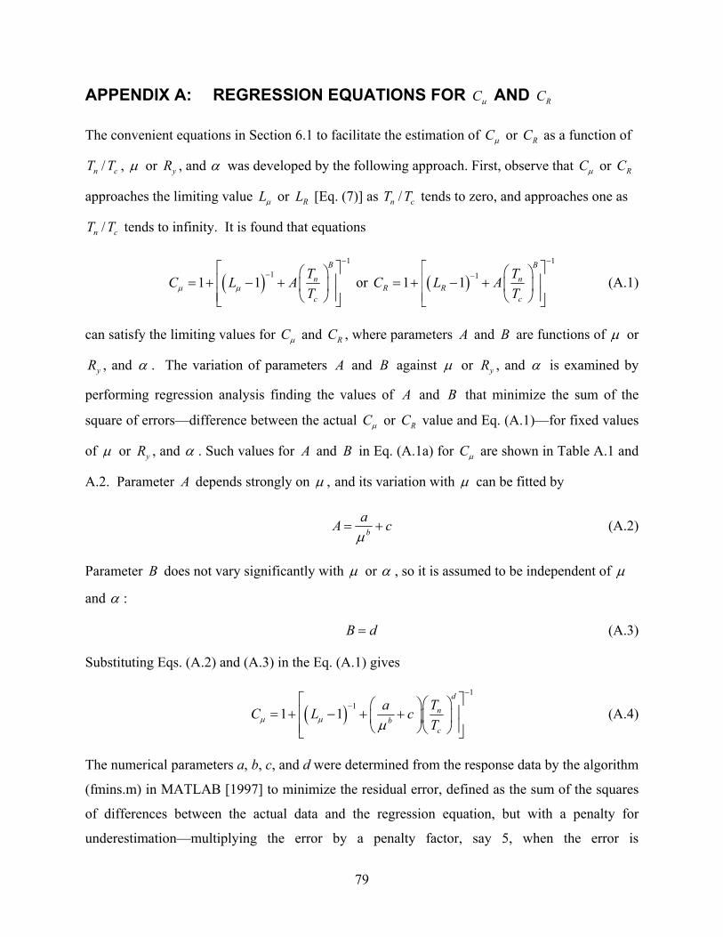
79

APPENDIX A: REGRESSION EQUATIONS FOR Cµ AND RC

The convenient equations in Section 6.1 to facilitate the estimation of Cµ or RC as a function of

/n cT T , µ or yR , and α was developed by the following approach. First, observe that Cµ or RC

approaches the limiting value Lµ or RL [Eq. (7)] as /n cT T tends to zero, and approaches one as

/n cT T tends to infinity. It is found that equations

( )1

11 1

B

n

c

TC L ATµ µ

−

− = + − +

or ( )1

11 1B

nR R

c

TC L AT

−

− = + − +

(A.1)

can satisfy the limiting values for Cµ and RC , where parameters A and B are functions of µ or

yR , and α . The variation of parameters A and B against µ or yR , and α is examined by

performing regression analysis finding the values of A and B that minimize the sum of the

square of errors—difference between the actual Cµ or RC value and Eq. (A.1)—for fixed values

of µ or yR , and α . Such values for A and B in Eq. (A.1a) for Cµ are shown in Table A.1 and

A.2. Parameter A depends strongly on µ , and its variation with µ can be fitted by

b

aA cµ

= + (A.2)

Parameter B does not vary significantly with µ or α , so it is assumed to be independent of µ

and α :

B d= (A.3)

Substituting Eqs. (A.2) and (A.3) in the Eq. (A.1) gives

( )1

11 1

d

nb

c

TaC L cTµ µ µ

−

− = + − + +

(A.4)

The numerical parameters a, b, c, and d were determined from the response data by the algorithm

(fmins.m) in MATLAB [1997] to minimize the residual error, defined as the sum of the squares

of differences between the actual data and the regression equation, but with a penalty for

underestimation—multiplying the error by a penalty factor, say 5, when the error is

80

underestimation to obtain a regression equation that is slightly conservative—: a = 72, b =2.2,

c = 1.6, and d = 1.5 using the LMSR data and a = 105, b = 2.3, c = 1.9, d = 1.7 using the data for

four (LMSR, LMLR, SMSR, and SMLR) ensembles; these parameter values are independent of

post-yield stiffness ratio, α .

A similar derivation for RC gives

( )1

11 1d

nR R b

y c

TaC L cR T

−

− = + − + +

(A.5)

Nonlinear regression analysis of the LMSR data led to a = 63, b = 2.3, c = 1.7, and d = 2.3, and

of the data for four ensembles of ground motion led to a = 61, b = 2.4, c = 1.5, and d = 2.4.

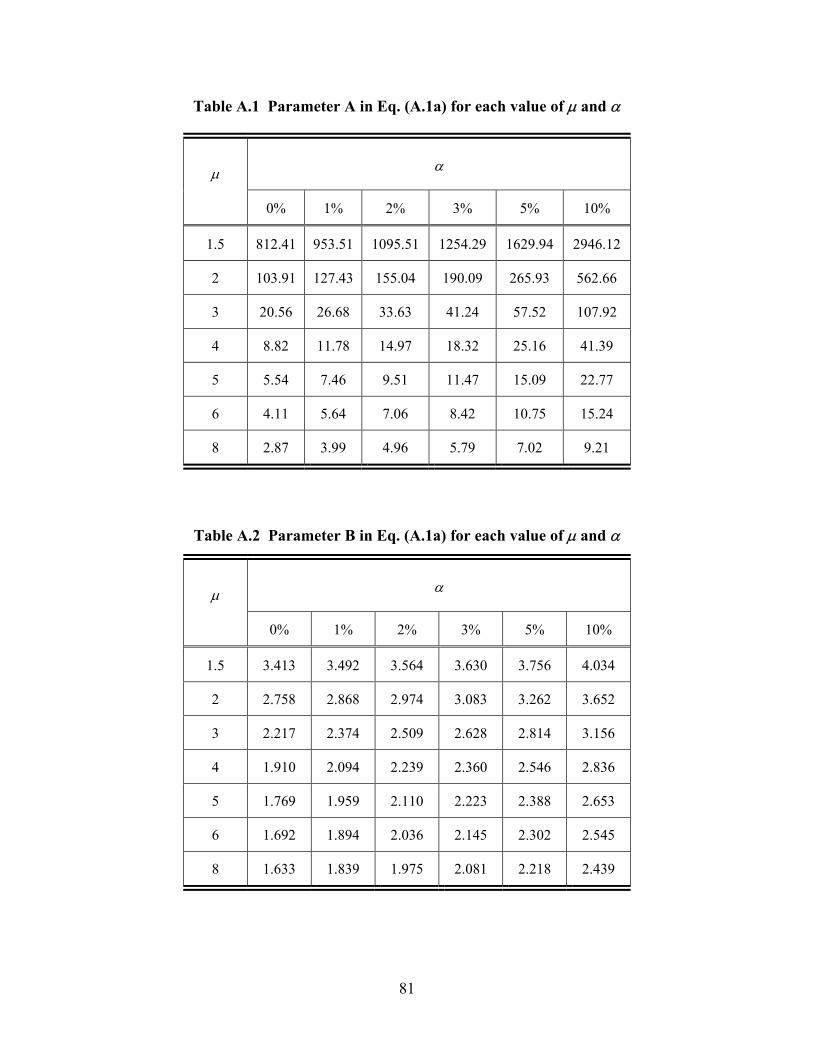
81

Table A.1 Parameter A in Eq. (A.1a) for each value of µ and α

µ α

0% 1% 2% 3% 5% 10%

1.5 812.41 953.51 1095.51 1254.29 1629.94 2946.12

2 103.91 127.43 155.04 190.09 265.93 562.66

3 20.56 26.68 33.63 41.24 57.52 107.92

4 8.82 11.78 14.97 18.32 25.16 41.39

5 5.54 7.46 9.51 11.47 15.09 22.77

6 4.11 5.64 7.06 8.42 10.75 15.24

8 2.87 3.99 4.96 5.79 7.02 9.21

Table A.2 Parameter B in Eq. (A.1a) for each value of µ and α

µ α

0% 1% 2% 3% 5% 10%

1.5 3.413 3.492 3.564 3.630 3.756 4.034

2 2.758 2.868 2.974 3.083 3.262 3.652

3 2.217 2.374 2.509 2.628 2.814 3.156

4 1.910 2.094 2.239 2.360 2.546 2.836

5 1.769 1.959 2.110 2.223 2.388 2.653

6 1.692 1.894 2.036 2.145 2.302 2.545

8 1.633 1.839 1.975 2.081 2.218 2.439

Inelastic Deformation Ratios for Design and Evaluation of Structures: Single-Degree-of-Freedom...

Documents

Transcript of Inelastic Deformation Ratios for Design and Evaluation of Structures: Single-Degree-of-Freedom...