Citation: Alhamayani, A.D.; Sun, Q.;

Hallinan, K.P. An Improved Method

to Estimate Savings from Thermal

Comfort Control in Residences from

Smart Wi-Fi Thermostat Data. Clean

Technol. 2022, 4, 395–406. https://

doi.org/10.3390/cleantechnol4020024

Academic Editor: Patricia Luis

Received: 5 April 2022

Accepted: 9 May 2022

Published: 12 May 2022

Publisher’s Note: MDPI stays neutral

with regard to jurisdictional claims in

published maps and institutional affil-

iations.

Copyright: © 2022 by the authors.

Licensee MDPI, Basel, Switzerland.

This article is an open access article

distributed under the terms and

conditions of the Creative Commons

Attribution (CC BY) license (https://

creativecommons.org/licenses/by/

4.0/).

clean technologies

Article

An Improved Method to Estimate Savings from ThermalComfort Control in Residences from Smart Wi-FiThermostat DataAbdulelah D. Alhamayani *, Qiancheng Sun and Kevin P. Hallinan *

Department of Mechanical & Aerospace Engineering, University of Dayton, Dayton, OH 45469-0238, USA;sunq11@udayton.edu* Correspondence: alhamayania1@udayton.edu (A.D.A.); kevin.hallinan@udayton.edu (K.P.H.)

Abstract: The net-zero global carbon target for 2050 needs both expansion of renewable energy andsubstantive energy consumption reduction. Many of the solutions needed are expensive. ControllingHVAC systems in buildings based upon thermal comfort, not just temperature, uniquely offers ameans for deep savings at virtually no cost. In this study, a more accurate means to quantify thesavings potential in any building in which smart WiFi thermostats are present is developed. Priorresearch by Alhamayani et al. leveraging such data for individual residences predicted cooling energysavings in the range from 33 to 47%, but this research was based only upon a singular data-basedmodel of indoor temperature. The present research improves upon this prior research by developingLSTM neural network models for both indoor temperature and humidity. Validation errors arereduced by nearly 22% compared to the prior work. Simulations of thermal comfort control for theresidences considered yielded potential savings in the range of 29–43%, dependent upon both solarexposure and insulation characteristics of each residence. This research paves the way for smart Wi-Fithermostat-enabled thermal comfort control in buildings of all types.

Keywords: smart Wi-Fi thermostats; long short-term memory; thermal comfort; PMV; MRT; relativehumidity; moving average; energy efficiency

1. Introduction

The Intergovernmental Panel for Climate Change (IPCC) has set a target of net-zerocarbon emissions by 2050 [1]. To get there, the International Energy Agency (IEA) estimatesthat clean energy investment by 2030 must increase three-fold to USD 4 trillion [2]. Technol-ogy innovation is certain to comprise a sizeable part of this investment [3]. One of the recenttechnologies proven to reduce the global energy demand are smart thermostats. In Europe,this technology, which has been adopted in over 1 million residences, has demonstrated 22%energy savings in this sector. If applied to all residences in Europe, total European carbondioxide (CO2) emissions can be reduced by around 5% [4]. Likewise, the US Governmenthas incentivized purchase of this technology for residences [5]. To date, 17% of residencesin the US now have such thermostats installed [6].

One application of smart Wi-Fi thermostats that has been identified is for use in con-trolling for thermal comfort rather than temperature. Several researchers have reportedpotential cooling energy savings from thermal comfort-driven and energy-aware HVACsystem control ranging from 4 to 32% in commercial buildings [7–10]. Ferreira et al., apply-ing neural network-based model for predictive thermal comfort control in a commercialbuilding, reported even greater estimated energy savings of more than 50% [11].

In residential buildings, Danassis et al. implemented artificial neural network andFuzzy Logic inference models to assess smart thermostat thermal comfort control. Theyestimated savings in the range of 18–40% [12]. Likewise, Lou et al. showed potentialcooling savings from similar control of up to 85% for a one-month period in the summer in

Clean Technol. 2022, 4, 395–406. https://doi.org/10.3390/cleantechnol4020024 https://www.mdpi.com/journal/cleantechnol

Clean Technol. 2022, 4 396

the Midwest, US [13]. Lastly, Alhamayani et al. expanded Lou et al.’s effort by accountingfor the influence of solar heat gain. They showed that solar contributions to cooling weresignificant. They reported more realistic cooling energy savings in the range of 33–47%.Further, they showed that the extent of the savings clearly depended upon the amount ofinsulation in a residence and exterior shading from other buildings and from trees [14]. Avery recent study by Sun et al. [15] demonstrated solar heat gain to the same housing setconsidered by Lou et al. [13] and Alhamayani et al. [14] is responsible for up to 72% of thecooling load in the residences considered [15].

The promise of implementing thermal comfort control in residences is increasing,especially with the global market for manufacturing smart thermostats predicted to increasefrom USD 88.7 billion to USD 228.2 billion from 2021 to 2027 [16]. This is expected totranslate to an estimated 1-2B new smart Wi-Fi thermostats entering the market. Such again in the market coupled with implementation of thermal comfort control could yieldsubstantial worldwide carbon reduction at virtually no cost.

The objective of this study is to build upon the prior research of Alhamayani et al. [14]to further improve the accuracy of estimation of the energy savings from implementingsmart thermostat thermal comfort control in residences. In comparison to the prior workof Lou et al. [13] and Alhamayani et al. [14], which assumed a constant indoor relativehumidity of 55%, this study accounts for this influence. The improvement in temperatureand relative humidity models is discussed. The impact of the addition of a relative humiditymodel to the estimation of the PMV value is documented. The estimated energy savingsfrom the current study is compared to the previous work by Alhamayani et al. [14].

2. Background

In general, residential and commercial buildings HVAC maintain human thermalcomfort through the maintenance of a set indoor temperature. However, human thermalcomfort depends on a number of other factors, including (i) other indoor environmentalfactors (relative humidity, air velocity, and mean radiant temperature, MRT); and (ii) oc-cupational factors (occupants’ age, gender, clothing, metabolic rate, and behavior, such asturning on/off the a/c or opening or closing windows) [17].

The well-known model utilized to quantify the thermal comfort of an occupant insidea controlled space is Fanger’s predicted mean vote (PMV). The PMV model generallyestimates the mean value of votes of occupants using a seven-point thermal sensationscale, ranging from −3 (much too cold) to +3 (much too hot). The optimal PMV range, assuggested in the ASHRAE 55 and ISO 7730 standards, is from −0.5 to +0.5 [18].

Prior research estimating savings from thermal comfort control in residences hasrelied upon different control strategies and algorithms. Azuatalam et al. [19] leverageda reinforcement learning agent to control the heating, ventilation, and air conditioning(HVAC) system in a commercial building. The power reduction realized from their controlstrategy reached a maximum of 50% weekly. Further, Park et al. [20] utilized a thermalcomfort-based controller to reduce the cooling energy of air-conditioning systems in aresidential building in Kuwait. Energy savings of 39.5% on a representative summer daywere documented. Another developed control strategy developed by Li et al. [21] basedon PMV-PDD smart thermostat control showed savings in a residential building of upto 11.5%.

The use of smart Wi-Fi PMV-based thermal comfort control is new. Only Lou et al. [13]and Alhamayani et al. [14] are the only known efforts that have relied upon this technology.Thus, in what follows in the results section, comparisons are made only with this prior work.

The proposed study here extends the prior work reported in Alhamayani et al. [14],following the framework established by Bac et al. [22], which posed a process for identifyingsuitable HVAC system options for a building by using building energy simulations. Here,these simulations are based upon data-based models of the energy systems. This priorwork of Alhamayani et al. relied upon a data-based machine learning model using archivedsmart thermostat data in addition to outdoor weather conditions and solar heating inputs

Clean Technol. 2022, 4 397

to predict internal temperature. The developed model was utilized to estimate a residence’sPMV and control the cooling load to achieve the optimal PMV at all times. The developedmodel considered the overall solar heat gain through the building envelope and fromsolar fenestration. However, as noted in Section 1, the prior research by Alhamayani et al.utilized an assumption of constant internal relative humidity (set to 55%). This paperagain leverages archived smart Wi-Fi thermostat data (internal temperature and relativehumidity and cooling status). It relies upon these data to develop data-based machinelearning models to predict both the internal temperature and relative humidity. It thenintegrates these models into a simulated thermal comfort control schema to evaluate moreaccurately the thermal comfort control for several residences with variable solar exposureand building envelope energy effectiveness. As a result, the predicted savings estimatesfrom thermal comfort control will be more realistic.

The remainder of the paper presents the methodology for developing a databasemachine learning model for both the internal temperature and relative humidity. It thenemploys the developed models into a simulated control of thermal comfort in severalresidences with variable solar exposure and energy effectiveness. It concludes with adiscussion of the results and implications of this research.

3. Methodology3.1. Data Collection3.1.1. Buildings, Smart Thermostats, Weather, and Solar Data

All the building characteristics, smart thermostats, weather, and solar data used in theearlier work by Lu et al. [13] and Alhamayani et al. [14] are utilized here. Table 1 documentsthe building characteristics of the residences used in this study.

Table 1. Residential building geometrical and energy characteristics data.

Home Characteristics/House No. 1 2 3 4 5

Afloor(m2 ) 54 84 54 59 45

Awall(m2 ) 159 187 156 152 149

Awindow(m2 ) 2–3 2–3 2–3 2–3 2–3

Rwall

(m2KW−1 ) 0.88 0.7 0.7 2.5 0.8

Rwindow

(m2KW−1 ) 0.35 0.35 0.35 0.35 0.35

RAttic

(m2KW−1 ) 3.87 2.15 1.1 6.69 3.17

AC power (kW) 10.5 8.8 10.5 10.5 12.25

3.1.2. Smart Thermostats Moving Averages

Prior work by Alhamayani et al. [14], Huang et al. [23], Sun et al. [15], and Lou et al. [13]developed models from archived time smart Wi-Fi measurements. The analysis describedhere uniquely considers possible inputs to the model described in Section 3.1.2, movingaverages of the smart Wi-Fi measured indoor temperature and relative humidity, as well asthe cooling demand status. The smoothing effect of using a moving average can improvethe prediction accuracy of machine learning models [24,25]. Different averaging windowtime intervals were considered for each of the major features (indoor temperature, indoorhumidity, and cooling demand status). An optimal moving average window associatedwith the lowest validation error from the models developed was determined for eachresidence. This ranged from 1 to 7 h, with the lower range associated with poor energyeffectiveness residences and the larger range associated with high energy effectivenesshouses. Table 2 lists the optimal interval moving averages for the selected features for eachresidence in this study.

Clean Technol. 2022, 4 398

Table 2. List of the optimal interval moving averages for the selected features for each residence.

HouseNumber

Moving Average Periodfor Temperature (h)

Moving Average Periodfor Relative Humidity (h)

Moving Average Periodfor Cooling Demand (h)

1 4 3 22 4 5 13 3 2 14 7 5 15 4 6 1

3.1.3. Data Preprocessing and Feature Engineering

The data pre-processing required here consisted of (i) creating uniformly spacedthermostat data from the actual event-based data. The thermostat data were archived onlywhen one of the measured features changed values. Additionally, the hourly weather andsolar data were synched with these data using linear interpolation. This data pre-processingwas described in earlier work [14].

In addition, Pearson’s correlation method was applied to eliminate highly correlatedfeatures (r > 0.9) [26]. Min–max normalization was applied as well. Sample smart Wi-Fithermostat features for one of the residences are shown in Table 3.

Table 3. Sample of synchronized Smart Wi-Fi thermostat, weather, and moving averages features forrelative humidity model.

IndoorRelative

Humidity(%)

OutdoorTemperature

(F)

Outdoor DewPoint

Temperature (F)

CoolingSetpoint

Temperature (F)

CoolingDemand

Status (0/1)

MovingAverageRelative

Humidity (%)

Moving AverageIndoor

Temperature (F)

Moving AverageCoolingDemand

(0–1)

61 79 70 75 0 61 74.7 054 78 65 75 0 53.8 75.5 0.256 83 66 72 1 58.8 72.1 0.53

3.2. Temperate and Relative Humidity Models DevelopmentLong Short-Term Memory (LSTM)

In this study, a deep learning neural network algorithm was considered for developingtwo separate dynamic models to predict the indoor temperature and relative humidityusing archived smart Wi-Fi thermostat data. The deep learning neural network developedemployed the long short-term memory (LSTM) neural network algorithm introducedby Hochreiter and Schmidhuber in 1997 [27]. The LSTM is a type of recurrent neuralnetwork (RNN). Much prior work has validated that LSTM performs better than RNN byovercoming the gradient vanishing problem or gradient explosion problem by forgettingthe previous observations having little influence over current predictions [27–30].

The architecture of the LSTM can be summarized as a combination of three types ofgates (forget gate, input gate, and output gate). LSTM advantages gates to add or removeinformation to the cell state [26]. The equation for all gates (forget ft, input it, and outputot) are:

ft = σ(

W f [ht−1, xt] + b f

)(1)

it = σ(Wi[ht−1, xt] + bi) (2)

ot = σ(Wo[ht−1, xt] + bo) (3)

The cell state Ct equation is:

Ct = tanh(Wc[ht−1, xt] + bC) (4)

Ct = ft ∗ Ct−1 + it ∗ Ct (5)

Clean Technol. 2022, 4 399

The output ht that comes out from the LSTM unit is:

ht = ot ∗ tanh(Ct) (6)

Generally, LSTM utilizes prior readings or values for all features (including the re-sponse variable) as predictors for the next response prediction by considering a lookbackperiod that controls the time period of prior readings or values used to forecast the nextresponse time step. To achieve the most effective predictive models and prevent overfittingissues, as well as speed up the computations, the data are batched. The batch size controlsthe number of training samples applied in one iteration and enables the propagation ofweightings across time.

The data used for model development, validation, and testing were split sequentiallyaccording to 72%/18%/10%. The batch size was set to be 128 in both models. Modelperformance was assessed utilizing R-squared (R2), mean absolute error (MAE), meanabsolute percentage error (MAPE), and root mean square error (RMSE).

3.3. The Effect of Multiple Predictive Models on PMVPredictive Mean Vote (PMV) Model

The quantification of thermal comfort in this study is obtained by “Fanger’s predictedmean vote (PMV) model” [17]. The levels of comfort are well defined in the seven-pointthermal sensation scale proposed by the American Society of Heating, Refrigerating, andAir-Conditioning Engineers (ASHRAE). The thermal sensation scale is: −3 (Cold), −2(Cool), −1 (Slightly cool), 0 (Neutral), +1 (Slightly warm), +2 (Warm), and +3 (Hot); and itrepresents the thermal sensation of a majority of people. A PMV index range between −0.5and +0.5 is most satisfactory to 80% of people [31].

The following values were set for the required parameters in the PMV calculation. Themetabolic rate, M, was set to range from 1 to 1.3 met, applicable to a residential activity. Theclothing insulation value, Icl, was set to range from 0.45 to 0.5 in the summer. The relative airvelocity term, var, was equated to range from 0.1 to 0.2 m/s, based upon the minimum valueaccepted by ASHRAE-55 [18]. The next subsections detail the estimation and validation ofthe MRT, respectively. Future work could potentially relax these assumptions.

The flowchart shown in Figure 1 summarizes how thermal comfort control wasenhanced from earlier work [14] and simulated in the housing set described in Table 1. It isclear the relative humidity model has been added to the thermal comfort control logic toadd more realistic PMV estimates to the previous work.

Clean Technol. 2022, 4 400Clean Technol. 2022, 4, FOR PEER REVIEW 6

Figure 1. Flowchart showing process for simulated thermal comfort control using two developed LSTM deep learning neural network models of internal relative humidity and temperature.

3.4. Potential Savings from PMV Control Utilizing Two Predictive Models The potential savings from thermal comfort control was determined by comparing

the simulated cooling using thermal comfort control to the actual cooling. The energy savings were determined by considering the effective duty cycle for the whole period and the cooling size of the residence’s HVAC, where the cooling duty cycle is defined as:

𝐸𝑓𝑓𝑒𝑐𝑡𝑖𝑣𝑒 𝐷𝑢𝑡𝑦 𝐶𝑦𝑐𝑙𝑒 = ∑(𝐶𝑜𝑜𝑙𝑖𝑛𝑔 𝑡𝑖𝑚𝑒) × (𝐶𝑜𝑜𝑙𝑖𝑛𝑔 𝐷𝑒𝑚𝑎𝑛𝑑 𝑆𝑡𝑎𝑡𝑢𝑠)∑ 𝑇𝑖𝑚𝑒 (7)

4. Results Results are presented to provide evidence that the use of two data-based models for

indoor temperature and relative humidity, coupled with the use of time-averaged

Figure 1. Flowchart showing process for simulated thermal comfort control using two developedLSTM deep learning neural network models of internal relative humidity and temperature.

3.4. Potential Savings from PMV Control Utilizing Two Predictive Models

The potential savings from thermal comfort control was determined by comparingthe simulated cooling using thermal comfort control to the actual cooling. The energysavings were determined by considering the effective duty cycle for the whole period andthe cooling size of the residence’s HVAC, where the cooling duty cycle is defined as:

E f f ective Duty Cycle = ∑(Cooling time)× (Cooling Demand Status)∑ Time

(7)

4. Results

Results are presented to provide evidence that the use of two data-based models forindoor temperature and relative humidity, coupled with the use of time-averaged quantitiesfor internal temperature, internal relative humidity, and cooling demand status, improvesthe estimation of savings from PVM-based thermal comfort control relative to prior workdone by Alhamayani et al. [14].

Clean Technol. 2022, 4 401

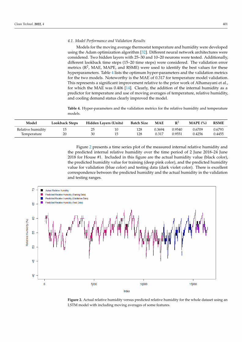
4.1. Model Performance and Validation Results

Models for the moving average thermostat temperature and humidity were developedusing the Adam optimization algorithm [32]. Different neural network architectures wereconsidered. Two hidden layers with 25–30 and 10–20 neurons were tested. Additionally,different lookback time steps (15–20 time steps) were considered. The validation errormetrics (R2, MAE, MAPE, and RSME) were used to identify the best values for thesehyperparameters. Table 4 lists the optimum hyper-parameters and the validation metricsfor the two models. Noteworthy is the MAE of 0.317 for temperature model validation.This represents a significant improvement relative to the prior work of Alhamayani et al.,for which the MAE was 0.406 [14]. Clearly, the addition of the internal humidity as apredictor for temperature and use of moving averages of temperature, relative humidity,and cooling demand status clearly improved the model.

Table 4. Hyper-parameters and the validation metrics for the relative humidity and temperaturemodels.

Model Lookback Steps Hidden Layers (Units) Batch Size MAE R2 MAPE (%) RSME

Relative humidity 15 25 10 128 0.3694 0.9540 0.6709 0.6793Temperature 20 30 15 128 0.317 0.9551 0.4256 0.4455

Figure 2 presents a time series plot of the measured internal relative humidity andthe predicted internal relative humidity over the time period of 2 June 2018–24 June2018 for House #1. Included in this figure are the actual humidity value (black color),the predicted humidity value for training (deep pink color), and the predicted humidityvalue for validation (blue color) and testing data (dark violet color). There is excellentcorrespondence between the predicted humidity and the actual humidity in the validationand testing ranges.

Clean Technol. 2022, 4, FOR PEER REVIEW 8

Figure 2. Actual relative humidity versus predicted relative humidity for the whole dataset using an LSTM model with including moving averages of some features.

Figure 3. Actual temperature versus predicted temperature for the whole dataset using an LSTM model obtained using the indoor relative humidity and moving averages as features.

Table 5. Validation matrices for all residences’ models.

Figure 2. Actual relative humidity versus predicted relative humidity for the whole dataset using anLSTM model with including moving averages of some features.

Clean Technol. 2022, 4 402

Figure 3 shows a similar plot for the enhanced temperature model, which uses as aninput the relative humidity. Included in this figure are plots of the measured temperaturedata (black color), and the predicted temperature data for the training (blue color), testing(green color), and validation (red color) data. The correspondence between the measureddata and the predictions in the validation and testing ranges is strikingly better than theprevious work of Lou et al. [13], Huang et al. [23], and Alhamayani et al. [14].

Clean Technol. 2022, 4, FOR PEER REVIEW 8

Figure 2. Actual relative humidity versus predicted relative humidity for the whole dataset using an LSTM model with including moving averages of some features.

Figure 3. Actual temperature versus predicted temperature for the whole dataset using an LSTM model obtained using the indoor relative humidity and moving averages as features.

Table 5. Validation matrices for all residences’ models.

Figure 3. Actual temperature versus predicted temperature for the whole dataset using an LSTMmodel obtained using the indoor relative humidity and moving averages as features.

Other considered residences detailed in Table 1 show similar results, as documentedin Table 5. As seen in this table, the MAE values for each of the residences considered rangefrom 0.317 to 0.412.

Table 5. Validation matrices for all residences’ models.

House No. MAE R2 MAPE (%) RSME

1 0.317 0.9551 0.4256 0.44552 0.319 0.9512 0.4313 0.45773 0.349 0.9457 0.4730 0.52304 0.396 0.9398 0.5285 0.57525 0.323 0.9498 0.4402 0.4607

Figure 4 presents a time series of the PMV values estimated for two cases: (a) a constantrelative humidity of 55% all over the time period, and (b) a relative humidity predictedusing the developed machine learning model for indoor humidity. The plot represents ahumid day in Dayton, Ohio, and demonstrates how the relative humidity affects the PMVestimations. It is clear that the more realistic higher relative humidity obtained here causes thePMV index estimation during the day (orange line) to be greater than the constant relativehumidity case considered by Alhamayani et al. [14]. Also shown is that for the more realisticrelative humidity model, additional cooling is required (see purple cooling demand status)in comparison to the case where a constant relative humidity is assumed. Thus, the modelimprovement almost certainly yields a more realistic perspective of the potential savings fromPMV thermal comfort control relative to typical temperature control of thermal comfort.

Clean Technol. 2022, 4 403

Clean Technol. 2022, 4, FOR PEER REVIEW 9

House No. MAE 𝐑𝟐 MAPE (%) RSME 1 0.317 0.9551 0.4256 0.4455 2 0.319 0.9512 0.4313 0.4577 3 0.349 0.9457 0.4730 0.5230 4 0.396 0.9398 0.5285 0.5752 5 0.323 0.9498 0.4402 0.4607

Figure 4 presents a time series of the PMV values estimated for two cases: (a) a constant relative humidity of 55% all over the time period, and (b) a relative humidity predicted using the developed machine learning model for indoor humidity. The plot represents a humid day in Dayton, Ohio, and demonstrates how the relative humidity affects the PMV estimations. It is clear that the more realistic higher relative humidity obtained here causes the PMV index estimation during the day (orange line) to be greater than the constant relative humidity case considered by Alhamayani et al. [14]. Also shown is that for the more realistic relative humidity model, additional cooling is required (see purple cooling demand status) in comparison to the case where a constant relative humidity is assumed. Thus, the model improvement almost certainly yields a more realistic perspective of the potential savings from PMV thermal comfort control relative to typical temperature control of thermal comfort.

Figure 4. Time series plot of real-time PMV value and cooling demand for the including relative humidity model and assuming relative humidity as constant value.

4.2. Potential Savings from PMV Control Utilizing Current Approach Reliant upon Both a Temperature and Humidity Predictive Model as Compared to Previous Approach Reliant upon Only a Predictive Model for Temperature

Figure 5 presents a comparison of the total cooling energy consumption for each of the eight residences over the time period from 2 June 2018 to 24 June 2018 for two cases: (i) thermal comfort control using only a predictive model for temperature (the demonstrated results were taken from the previous work done by Alhamayani et al. [14]); and (ii) thermal comfort control using two predictive models (relative humidity and temperature). The blue bars represent the cooling energy consumption for case (i), while the red bars represent the cooling energy consumption for case (ii). It is clear that the addition of a humidity model yields greater cooling energy consumption in comparison to similar predictions based upon an assumed constant indoor relative humidity.

Figure 4. Time series plot of real-time PMV value and cooling demand for the including relativehumidity model and assuming relative humidity as constant value.

4.2. Potential Savings from PMV Control Utilizing Current Approach Reliant upon Both aTemperature and Humidity Predictive Model as Compared to Previous Approach Reliant uponOnly a Predictive Model for Temperature

Figure 5 presents a comparison of the total cooling energy consumption for each ofthe eight residences over the time period from 2 June 2018 to 24 June 2018 for two cases:(i) thermal comfort control using only a predictive model for temperature (the demonstratedresults were taken from the previous work done by Alhamayani et al. [14]); and (ii) thermalcomfort control using two predictive models (relative humidity and temperature). The bluebars represent the cooling energy consumption for case (i), while the red bars representthe cooling energy consumption for case (ii). It is clear that the addition of a humiditymodel yields greater cooling energy consumption in comparison to similar predictionsbased upon an assumed constant indoor relative humidity.

Clean Technol. 2022, 4, FOR PEER REVIEW 10

Figure 5. Cooling energy consumption for the residences described in Table 1 for two cases: (1) PMV control with one predictive model (temperature) (Alhamayani et al. [14]) and (2) PMV control with two predictive models (relative humidity and temperature).

Figure 6, which shows lines chart for the relative humidity measured in selected residences over the time period covered, sheds some light on the differences seen in Figure 5. Also included in this plot is the outdoor relative humidity. It is shown that the indoor relative humidity tends to a damped tracking of the outdoor relative humidity. Notable is that one of the buildings (House No. 7) generally has lower relative humidity values than the other houses. The reason for this is likely because the air leakage in this newer residence designed to Energy Star criteria is significantly lower. It is certain that the thermal comfort experienced by residents during this time period was negatively influenced by indoor humidity as the simulated relative humidity is greater than the 55% constant value assumed in the prior study. Subsequently, the energy savings from thermal comfort control are lower than was predicted from the previous work done by Alhamayani et al. [14], as documented for each of the residences in Table 6. The energy savings from thermal comfort control for the residences considered ranged from 29 to 43%, in contrast to savings ranging from 33 to 47% in the prior work by Alhamayani et al. [14].

Figure 5. Cooling energy consumption for the residences described in Table 1 for two cases: (1) PMVcontrol with one predictive model (temperature) (Alhamayani et al. [14]) and (2) PMV control withtwo predictive models (relative humidity and temperature).

Clean Technol. 2022, 4 404

Figure 6, which shows lines chart for the relative humidity measured in selectedresidences over the time period covered, sheds some light on the differences seen inFigure 5. Also included in this plot is the outdoor relative humidity. It is shown that theindoor relative humidity tends to a damped tracking of the outdoor relative humidity.Notable is that one of the buildings (House No. 7) generally has lower relative humidityvalues than the other houses. The reason for this is likely because the air leakage in thisnewer residence designed to Energy Star criteria is significantly lower. It is certain thatthe thermal comfort experienced by residents during this time period was negativelyinfluenced by indoor humidity as the simulated relative humidity is greater than the 55%constant value assumed in the prior study. Subsequently, the energy savings from thermalcomfort control are lower than was predicted from the previous work done by Alhamayaniet al. [14], as documented for each of the residences in Table 6. The energy savings fromthermal comfort control for the residences considered ranged from 29 to 43%, in contrast tosavings ranging from 33 to 47% in the prior work by Alhamayani et al. [14].

Clean Technol. 2022, 4, FOR PEER REVIEW 11

Figure 6. Actual outdoor relative humidity versus selected residences’ relative humidity for the whole dataset.

Table 6. Savings from the implementation of thermal comfort control for the residences considered in study.

Model Savings/House No. 1 2 3 4 5 Temperature model only 40% 47% 46% 33% 40%

Relative humidity and temperature models

36% 42% 43% 29% 31%

5. Conclusions The current work was on the prior work introduced by Lou et al. [13] and

Alhamayani et al. [14]. In comparison, this study demonstrates a more realistic simulation of smart thermostat-based thermal comfort control in residences through consideration of a variable relative humidity. Greater accuracy was also achieved by using moving averages for the critical predictors (indoor temperature, indoor humidity, and cooling demand status). With improved accuracy models, the estimated cooling energy savings are more realistically predicted to be in the range of 29–43%, where the greater potential savings are achievable in residences with poor energy effectiveness.

The significance of this research is (1) that significant cooling energy and carbon savings could be achieved with virtually no cost and (2) that this approach could be used today in any residence with smart Wi-Fi thermostats to estimate savings from thermal comfort control. The next step has to be implementation of thermal comfort control at scale.

This work also has potential policy implications. As the smart Wi-Fi thermostat posed PMV thermal comfort control has a demonstrated potential to save energy and reduce carbon emissions at virtually no cost, it is reasonable to imagine policies emerging to set thermostat control standards based upon thermal comfort control. The establishment of standards for this would certainly be the domain of organizations such as ASHRAE in the US and REHVA in Europe. Of course, any standard emerging should not be draconian. Elderly people and people with health conditions may not be able to tolerate “stretch” PMV comfort levels to yield greater savings.

Figure 6. Actual outdoor relative humidity versus selected residences’ relative humidity for thewhole dataset.

Table 6. Savings from the implementation of thermal comfort control for the residences consideredin study.

Model Savings/House No. 1 2 3 4 5

Temperature model only 40% 47% 46% 33% 40%Relative humidity and temperature models 36% 42% 43% 29% 31%

5. Conclusions

The current work was on the prior work introduced by Lou et al. [13] and Alhamayaniet al. [14]. In comparison, this study demonstrates a more realistic simulation of smartthermostat-based thermal comfort control in residences through consideration of a variablerelative humidity. Greater accuracy was also achieved by using moving averages for thecritical predictors (indoor temperature, indoor humidity, and cooling demand status). Withimproved accuracy models, the estimated cooling energy savings are more realisticallypredicted to be in the range of 29–43%, where the greater potential savings are achievablein residences with poor energy effectiveness.

Clean Technol. 2022, 4 405

The significance of this research is (1) that significant cooling energy and carbonsavings could be achieved with virtually no cost and (2) that this approach could be usedtoday in any residence with smart Wi-Fi thermostats to estimate savings from thermalcomfort control. The next step has to be implementation of thermal comfort control at scale.

This work also has potential policy implications. As the smart Wi-Fi thermostat posedPMV thermal comfort control has a demonstrated potential to save energy and reducecarbon emissions at virtually no cost, it is reasonable to imagine policies emerging to setthermostat control standards based upon thermal comfort control. The establishment ofstandards for this would certainly be the domain of organizations such as ASHRAE in theUS and REHVA in Europe. Of course, any standard emerging should not be draconian.Elderly people and people with health conditions may not be able to tolerate “stretch” PMVcomfort levels to yield greater savings.

The limitations of this research are clearly seen. The shading and actual solar fenes-trations can affect the developed MRT estimations accuracy. It is complex to figure outthe time that a residence is shaded by a tree or surrounded residence. However, the studydeveloped by Sun et al. [15] can be modified to let smart thermostats understand whenthe house is receiving solar irradiances or not, which could help this proposed technologyovercome this limitation. Other limitations, such as the number and type of windows, canalso be overcome by utilizing the same work done by Sun et al. [15] with knowledge ofthe total solar transmitted into the house and using in estimating the MRT value for thewhole residence.

Author Contributions: Conceptualization, A.D.A. and K.P.H.; methodology, A.D.A., K.P.H., and Q.S.;software, A.D.A. and Q.S.; validation, A.D.A., Q.S. and K.P.H.; formal analysis, A.D.A.; investigation,A.D.A. and K.P.H.; resources, A.D.A. and K.P.H.; data curation, K.P.H.; writing—original draftpreparation, A.D.A.; writing—review and editing, A.D.A., K.P.H. and Q.S.; visualization, A.D.A. andQ.S.; supervision, A.D.A. and K.P.H.; project administration, A.D.A. and K.P.H. All authors have readand agreed to the published version of the manuscript.

Funding: This research received no specific grant from any funding agency in the public, commercial,or not-for-profit sectors.

Institutional Review Board Statement: Not applicable.

Informed Consent Statement: Not applicable.

Data Availability Statement: Not applicable.

Acknowledgments: Emerson Sensi is acknowledged for their permission to access smart Wi-Fi datafor the housing set considered in this study.

Conflicts of Interest: The authors declare no conflict of interest.

References1. Masson-Delmotte, V.; Zhai, H.-O.P.; Pörtner, D.; Roberts, J.; Skea, P.R.; Shukla, A.; Pirani, W.; Moufouma-Okia, C.; Péan,

R.; Pidcock, S.; et al. (Eds.) Summary for Policymakers. In Global Warming of 1.5 ◦C. An IPCC Special Report on the Impactsof Global Warming of 1.5 ◦C above Pre-Industrial Levels and Related Global Greenhouse Gas Emission Pathways, in the Context ofStrengthening the Global Response to the Threat of Climate Change, Sustainable Development, and Efforts to Eradicate Poverty; IPCC:Geneva, Switzerland, 2018.

2. Dolf, G.; Ricardo, G.; Gayathri, P.; Rodrigo, L.; Rabea, F.; Ulrike, L.; Xavier, C.; Diala, H.; Bishal, P. World Energy TransitionsOutlook—1.5 ◦C Pathway; International Renewable Energy Agency: Abu Dhabi, United Arab Emirates, 2021.

3. Dolf, G. Global Energy Transformation—A Roadmap to 2050; International Renewable Energy Agency: Abu Dhabi, United ArabEmirates, 2018.

4. New Report from Gemserv and Tado Shows Smart Thermostats Most Cost Effective and Scalable Way to Decarbonise Homes inthe EU’s Green Deal Renovation Wave. Business Wire. 21 October 2021. Available online: https://www.businesswire.com/news/home/20211021005179/en/New-Report-from-Gemserv-and-tado%C2%B0-Shows-Smart-Thermostats-Most-Cost-Effective-and-Scalable-Way-to-Decarbonise-Homes-in-the-EU%E2%80%99s-Green-Deal-Renovation-Wave (accessed on 4 February 2022).

5. Biden’s Green Procurement Executive Order, Smart Thermostats, and More. Resources for the Future. Available online:https://www.resources.org/on-the-issues/bidens-green-procurement-executive-order-smart-thermostats-and-more/ (accessedon 4 February 2022).

Clean Technol. 2022, 4 406

6. Liu, J. Ownership of Smart Thermostat Reaches 13% in the U.S. The Comprehensive Security Industry Platform. Available online:https://www.asmag.com/showpost/26461.aspx (accessed on 22 January 2018).

7. Masoso, O.; Grobler, L.J. The dark side of occupants’ behaviour on building energy use. Energy Build. 2010, 42, 173–177. [CrossRef]8. Vakiloroaya, V.; Samali, B.; Fakhar, A.; Pishghadam, K. A review of different strategies for HVAC energy saving. Energy Convers.

Manag. 2014, 77, 738–754. [CrossRef]9. Ghahramani, A.; Dutta, K.; Yang, Z.; Ozcelik, G.; Becerik-Gerber, B. Quantifying the influence of temperature setpoints, building

and system features on energy consumption. In Proceedings of the Winter Simulation Conference (WSC), Huntington Beach, CA,USA, 6–9 December 2015; IEEE: Piscataway, NJ, USA, 2015; pp. 1000–1011.

10. Ghahramani, A.; Dutta, K.B. Becerik-gerber, energy trade off analysis of optimized daily temperature setpoints. J. Build. Eng.2018, 19, 584–591. [CrossRef]

11. Ferreira, P.; Ruano, A.; Silva, S.; Conceição, E. Neural networks based predictive control for thermal comfort and energy savingsin public buildings. Energy Build. 2012, 55, 238–251. [CrossRef]

12. Danassis, P.; Siozios, K.; Korkas, C.; Soudris, D.; Kosmatopoulos, E. A low-complexity control mechanism targeting smartthermostats. Energy Build. 2017, 139, 340–350. [CrossRef]

13. Lou, R.; Hallinan, K.; Huang, K.; Reissman, T. Smart Wifi Thermostat-Enabled Thermal Comfort Control in Residences. Sustain-ability 2020, 12, 1919. [CrossRef]

14. Alhamayani, A.D.; Sun, Q.; Hallinan, K.P. Estimating Smart Wi-Fi Thermostat-Enabled Thermal Comfort Control Savings for AnyResidence. Clean Technol. 2021, 3, 743–760. [CrossRef]

15. Sun, Q.; Alhamayani, A.; Huang, K.; Hao, L.; Hallinan, K.; Ghareeb, A. Smart Wi-Fi physics-informed thermostat enabledestimation of residential passive solar heat gain for any residence. Energy Build. 2022, 261, 111934. [CrossRef]

16. Smart Manufacturing Market. Market Research Firm. Available online: https://www.marketsandmarkets.com/Market-Reports/smart-manufacturing-market-105448439.html (accessed on 5 February 2022).

17. Fanger, P.O. Thermal Comfort: Analysis and Applications in Environmental Engineering; McGraw-Hill: New York, NY, USA, 1970.18. American Society of Heating, Refrigerating and Air-Conditioning Engineers (ASHRAE). Thermal Environmental Conditions for

Human Occupancy, ANSI/ASHRAE Standard; American Society of Heating, Refrigerating and Air-Conditioning Engineers, Inc.:Peachtree Corners, GA, USA, 2012.

19. Azuatalam, D.; Lee, W.-L.; de Nijs, F.; Liebman, A. Reinforcement learning for whole-building HVAC control and demandresponse. Energy AI 2020, 2, 100020. [CrossRef]

20. Park, J.; Kim, T.; Lee, C.-S. Development of Thermal Comfort-Based Controller and Potential Reduction of the Cooling EnergyConsumption of a Residential Building in Kuwait. Energies 2019, 12, 3348. [CrossRef]

21. Li, Y.; De La Ree, J.; Gong, Y. The Smart Thermostat of HVAC Systems Based on PMV-PPD Model for Energy Efficiency andDemand Response. In Proceedings of the 2018 2nd IEEE Conference on Energy Internet and Energy System Integration (EI2),Beijing, China, 20–22 October 2018; pp. 1–6. [CrossRef]

22. Ugur, B.; Khalid, A.; Cihan, T. A comprehensive evaluation of the most suitable HVAC system for an industrial building by usinga hybrid building energy simulation and multi criteria decision making framework. J. Build. Eng. 2021, 37, 102153. [CrossRef]

23. Huang, K.; Hallinan, K.; Lou, R.; Alanezi, A.; Alshatshati, S.; Sun, Q. Self-Learning Algorithm to Predict Indoor Temperature andCooling Demand from Smart WiFi Thermostat in a Residential Building. Sustainability 2020, 12, 7110. [CrossRef]

24. Brownlee, J. Moving Average Smoothing for Data Preparation and Time Series Forecasting in Python. Machine Learning Mastery.14 August 2020. Available online: https://machinelearningmastery.com/moving-average-smoothing-for-time-series-forecasting-python/ (accessed on 4 April 2022).

25. KumarI, A. Moving Average Method for Time-Series Forecasting. Data Analytics. 4 April 2021. Available online: https://vitalflux.com/moving-average-method-for-time-series-forecasting/ (accessed on 4 April 2022).

26. Xu, P.; Han, S.; Huang, H.; Qin, H. Redundant features removal for unsupervised spectral feature selection algorithms: Anempirical study based on nonparametric sparse feature graph. Int. J. Data Sci. Anal. 2018, 8, 77–93. [CrossRef]

27. Hochreiter, S.; Schmidhuber, J. Long short-term memory. Neural Comput. 1997, 9, 1735–1780. [CrossRef] [PubMed]28. Hu, Y.; Huber, A.E.; Anumula, J.; Liu, S. Overcoming the vanishing gradient problem in plain recurrent networks. arXiv 2018,

arXiv:1801.06105.29. Corentin, T.; Yann, O. Can Recurrent Neural Networks Warp Time? Available online: https://arxiv.org/pdf/1804.11188.pdf

(accessed on 5 February 2022).30. Scott, W.; Thomas, P.; John, H.; Jonathan, L.R.; Les, A. Full-Capacity Unitary Recurrent Neural Networks. Available online:

https://proceedings.neurips.cc/paper/2016/file/d9ff90f4000eacd3a6c9cb27f78994cf-Paper.pdf (accessed on 5 February 2022).31. What Is PMV? What Is PPD? Basics of Thermal Comfort. SimScale. 14 June 2021. Available online: https://www.simscale.com/

blog/2019/09/what-is-pmv-ppd/ (accessed on 5 February 2022).32. Kingma, D.P.; Ba, J. Adam: A Method for Stochastic Optimization. Available online: https://arxiv.org/abs/1412.6980 (accessed

on 5 February 2022).