Refund to Savings 2013: Comprehensive Report on a 2015 large-scale tax-time savings program

REFUND TO SAVINGS 2013:COmpREhENSIVE REpORT ON A

lARGE-SCAlE TAx-TImE SAVINGS pROGRAm2015

CSD Research Report No. 15-06

CSD.WUSTL.EDU // 1

CONTENTS

Illustrations ....................................................................2Acknowledgments and Disclaimer ...................................4Executive Summary ........................................................5

part One The Refund to Savings ExperimentI. Overview ...............................................................9II. Background ..........................................................11III. Research Design ...................................................15IV. Participant Characteristics ...................................21

part Two Research Findings: The Experiment

V. Impact of R2S at Tax Time ....................................27VI. The Impact of R2S 6 Months After Filing ...............31

part Three Research Findings: Descriptive Results

VII. Receipt and Utilization of Tax Refunds ..................37VIII. The Financial Lives of LMI Households ..................43IX. Coping With Lack of Savings .................................47X. Behavioral Insights ...............................................49XI. Conclusion ...........................................................51

References ...................................................................53Authors .........................................................................58Suggested Citation ........................................................58Contact Us ....................................................................58

REFUND TO SAVINGS 2013: COmpREhENSIVE REpORT ON A lARGE-SCAlE TAx-TImE SAVING pROGRAm

By Michal Grinstein-Weiss, Dana C. Perantie, Blair D. Russell, Krista Comer, Samuel H. Taylor, Lingzi Luo, Clinton Key, & Dan Ariely

CSD Research Report No. 15-06

2 // WINTER 2015

IllUSTRATIONS

FIgURES

Figure 1 A screenshot within TurboTax Freedom Edition showing an Emergency prompt paired with a prepopulated savings suggestion anchored at 25% of the tax refund ................ 16

Figure 2 Overview of participant recruitment and inclusion in analyses ........................................... 20

Figure 3 Mean federal refund varies by date filing began (n = 853,674) ............................................ 23Figure 4 Percentages of participants who deposited any refund into savings vehicles by

test period......................................................................................................................... 27Figure 5 Probability of depositing any refund into a savings vehicle at tax time by anchor

amount, based on regression estimates (n = 468,947) ......................................................... 28Figure 6 Probability of depositing any refund into savings vehicle at tax time by prompt

message, based on regression estimates (n = 468,985) ....................................................... 28Figure 7 Percentages of participants who split any refunds into savings vehicles by test

period ............................................................................................................................... 28Figure 8 Average dollar amounts of refunds deposited into savings vehicles by test

period ............................................................................................................................... 29Figure 9 Dollar amount deposited into savings vehicle at tax time by anchor amount,

based on regression estimates (n = 468,947) ...................................................................... 30Figure 10 Dollar amount deposited into savings vehicle at tax time by prompt message,

based on regression estimates (n = 468,985) ...................................................................... 30Figure 11 Probability of saving refund for 6 months by anchor amount, based on regression

estimates (n = 4,172) ......................................................................................................... 31Figure 12 Probability of saving for 6 months by prompt, based on regression estimates

(n = 4,172) ......................................................................................................................... 31Figure 13 Percentage of refund saved for 6 months by anchor amount, based on regression

estimates (n = 4,833) .......................................................................................................... 32Figure 14 Percentage of refund saved for 6 months by prompt, based on regression

estimates (n = 4,833) ......................................................................................................... 32Figure 15 Percentage of survey respondents who say they could come up with $2,000 in

an emergency by anchor amount, based on regression estimates (n = 4,727) ...................... 32Figure 16 Percentage of respondents who say they could come up with $2,000 in an

emergency by prompt, based on regression estimates (n = 4,727) ...................................... 33Figure 17 Percentages of HFS1 participants interested in receiving their tax refunds in

alternative ways (n = 17,898) ............................................................................................. 37Figure 18 Percentages of HFS1 participants interested in receiving their tax refunds in

alternative ways by banked status (16,940 banked, 961 unbanked) .................................... 38Figure 19 Allocation of tax refunds: Intention at tax time versus reported use 6 months

later (n = 7,772) ................................................................................................................ 39Figure 20 Reported use of the tax refund varies according to size of the refund (HFS2,

n = 7,655) .......................................................................................................................... 39Figure 21 Purposes for saving tax refund among HFS2 participants who reported saving

CSD.WUSTL.EDU // 3

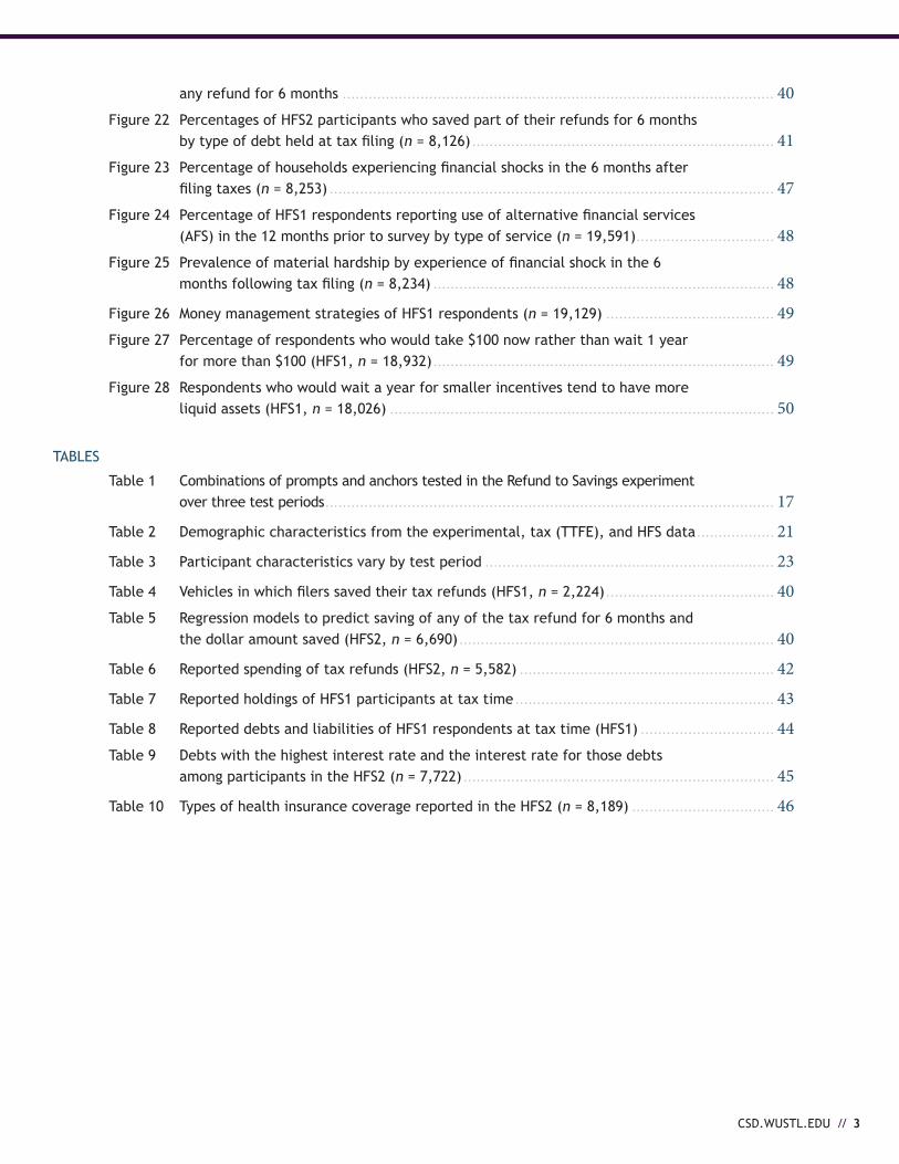
any refund for 6 months .................................................................................................... 40Figure 22 Percentages of HFS2 participants who saved part of their refunds for 6 months

by type of debt held at tax filing (n = 8,126) ...................................................................... 41Figure 23 Percentage of households experiencing financial shocks in the 6 months after

filing taxes (n = 8,253) ....................................................................................................... 47Figure 24 Percentage of HFS1 respondents reporting use of alternative financial services

(AFS) in the 12 months prior to survey by type of service (n = 19,591) ................................ 48Figure 25 Prevalence of material hardship by experience of financial shock in the 6

months following tax filing (n = 8,234) ............................................................................... 48

Figure 26 Money management strategies of HFS1 respondents (n = 19,129) ....................................... 49Figure 27 Percentage of respondents who would take $100 now rather than wait 1 year

for more than $100 (HFS1, n = 18,932) ............................................................................... 49Figure 28 Respondents who would wait a year for smaller incentives tend to have more

liquid assets (HFS1, n = 18,026) ......................................................................................... 50

TABLES

Table 1 Combinations of prompts and anchors tested in the Refund to Savings experiment over three test periods ........................................................................................................ 17

Table 2 Demographic characteristics from the experimental, tax (TTFE), and HFS data .................. 21

Table 3 Participant characteristics vary by test period ................................................................... 23

Table 4 Vehicles in which filers saved their tax refunds (HFS1, n = 2,224) ....................................... 40Table 5 Regression models to predict saving of any of the tax refund for 6 months and

the dollar amount saved (HFS2, n = 6,690) ......................................................................... 40

Table 6 Reported spending of tax refunds (HFS2, n = 5,582) ........................................................... 42

Table 7 Reported holdings of HFS1 participants at tax time ............................................................ 43

Table 8 Reported debts and liabilities of HFS1 respondents at tax time (HFS1) ............................... 44Table 9 Debts with the highest interest rate and the interest rate for those debts

among participants in the HFS2 (n = 7,722) ........................................................................ 45

Table 10 Types of health insurance coverage reported in the HFS2 (n = 8,189) ................................. 46

4 // WINTER 2015

ACkNOwlEDGmENTS

The Center for Social Development at Washington University in St. Louis gratefully acknowledges the funders who made the Refund to Savings initiative possible: the Ford Foundation; the Annie E. Casey Foundation; Intuit, Inc.; the Intuit Financial Freedom Foundation; the University of North Carolina at Chapel Hill; and an anonymous donor. We thank them for their support but acknowledge that the findings and conclusions presented in this report are those of the authors alone, and do not necessarily reflect the opinions of the foundations or the donors. The research team extends special thanks to Amy Brown and Frank Degiovanni with the Ford Foundation, and to Beadsie Woo with the Annie E. Casey Foundation. We appreciate their invaluable feedback, direction, and support at every stage of this process.

Refund to Savings would not exist without the commitment of Intuit, Inc., and particularly Intuit’s Consumer Tax group. We appreciate the executive sponsorship of Phillip Poirier as well as direction and insight from David Williams. We also appreciate the efforts of key contributors from the TurboTax development, marketing, and analytics teams, which have worked diligently on the planning and implementation of the experiment: Joe Lillie, Sacha Adams, Piritta Luoto, Julia Zhuang, Topher Stevenson, Annette Hoffard, and Kathy Kirkendall. We thank the Intuit Financial Freedom Foundation for providing the TurboTax Freedom Edition platform and Susan Mason for her contributions.

The Refund to Savings Advisory Committee, which includes Ray Boshara, Amy Brown, Keith Ernst, Tim Flacke, Julian Jamison, David Rothstein, Michael Sherraden, Jennifer Tescher, and Beadsie Woo, has provided outstanding advice throughout the initiative.

Lastly, we thank the thousands of tax filers who participated in the research surveys and shared their personal financial information with us. We hope this research will generate evidence that proves useful in developing policies aimed at helping low- and moderate-income households to increase their financial security and mobility.

DISClAImER

Statistical compilations disclosed in this document relate directly to the bona fide research of and public policy dis-cussions concerning the promotion of increased savings in connection with the tax compliance process. All compila-tions are anonymous and do not disclose cells containing data from fewer than 10 tax returns. IRS Reg. 301.7216

CSD.WUSTL.EDU // 5

The Refund to Savings (R2S) initiative, a product of a unique collaboration among partners from academia and industry, seeks to improve

the financial security of low- and middle-income (LMI) households by promoting saving of federal tax refunds. Researchers from Washington University in St. Louis and Duke University have worked with Intuit, Inc., the maker of TurboTax software, to design and test scalable interventions that encourage tax filers to save a portion of their federal tax refunds and that streamline the process of depositing refunds directly to savings vehicles. These computer-based interventions are low cost and low touch; that is, only a minimal investment of personnel is required to deliver the interventions to great numbers of people.

The annual occasion of filing taxes (“tax time”) presents a unique opportunity to encourage and facilitate saving behavior at a time when people anticipate receiving lump sums—tax refunds—beyond usual income. In 2013 (tax year 2012), approximately 680,000 refund-eligible tax filers participated in the R2S experiment, which Intuit embedded in TurboTax Freedom Edition (TTFE), the tax-preparation software that Intuit offers for free to qualified LMI households. The experiment’s randomized controlled design enables rigorous evaluation of a variety of interventions to increase the number of savers and the dollar amounts saved. This report presents results from an evaluation of R2S interventions in 2013.

Principles of behavioral economics informed the content of messages and the format of these interventions. In addition, the experiment was designed to make saving a salient default option. We tested two main behavioral mechanisms in varying combinations throughout the 2013 tax-filing season: (a) motivational prompts and (b) suggested savings amounts (anchors).

Six primary research questions are addressed by the R2S experiment:

• Can behavioral economics techniques increase the number of people who deposit to savings at tax time?

• Can R2S encourage filers to split their refund, allocating a portion to savings?

• Does R2S increase the amount of money deposited into savings at tax time?

• Do R2S interventions increase the number of people who save their refund for 6 months?

• Can R2S increase the proportion of refund saved 6 months?

• What can R2S administrative and survey data tell us about the financial lives of LMI households?

Data for this evaluation come from two sources. Data on income, tax credits and deductions claimed, tax

ExECUTIVE SUmmARy

Refund to Savings 2013:

Comprehensive Report on a large-Scale Tax-Time Saving program

By Michal Grinstein-Weiss, Dana C. Perantie, Blair D. Russell, Krista Comer, Samuel H. Taylor, Lingzi Luo, Clinton Key, & Dan Ariely

6 // WINTER 2015

refund amount, and the participant’s chosen method for receipt of the refund (e.g., via direct deposit into a savings account) are collected by the TTFE software. This information is complemented by data from two waves of a survey administered by the researchers. Immediately after submitting their tax returns, 20,816 filers responded to an invitation to take a detailed Household Financial Survey, which thoroughly examined assets, liabilities, intended use of tax refunds, product preferences, behavioral characteristics, and demographic traits. Six months later, 8,484 of those respondents participated in the second wave of the survey and reported on their actual use of the refunds. Data from the longitudinal survey also offer useful insights into the financial lives of LMI households. It is important to understand the context in which those households are trying to save and the methods of coping with contingencies when savings are not available. Such knowledge is key in designing effective strategies to encourage saving. Details on the balance sheets, tax credits taken, and predictors of saving behavior can inform researchers and policymakers interested in improving the financial well-being of LMI households. The data collected via the TTFE software and Household Financial Survey enable us to assess whether the R2S interventions’ effects on savings outcomes persist 6 months after filing.

Results from the R2S experiment show that minor design changes informed by behavioral economics can increase both the number of tax filers who deposit a portion of their refund into savings vehicles and the amount saved. We estimate that an additional 4,800 tax filers deposited some part of their refund into a savings vehicle because of the R2S interventions and that R2S interventions increased the amount saved by approximately 6 million dollars. Although the effects of the tested interventions are modest, the reach is broad and cumulatively substantial for such a low-touch, low-cost approach. The potential impact on individual households may be considerable.

It is noteworthy that the R2S interventions continued to affect the probability of saving and the percentage of the refund saved for at least 6 months after participants filed their taxes. In particular, we find that high anchoring (i.e., suggesting that filers save 50% or 75% of their refund) significantly increases the probability of saving and the percentage of the refund saved.

The two-wave Household Financial Survey provides valuable insights into the financial situations and challenges of LMI households. We find that nearly two thirds of households used some part of their tax refunds to pay down debt, and more than one in 10 households has already mentally allocated next year’s

refund for paying down debt. By several measures, our findings suggest that debt repayment, even more than spending, competes with the ability to save.

A close look at the balance sheets of these LMI households reveals evidence of a challenging financial environment. The median value of nonproperty assets was $1,300, and the median value of nonproperty liabilities was $10,000. If one includes property holdings as well as debt and other liabilities, the median net worth in this population was negative ($1,100). Student debt plays an important role in these households: Over half of households reported debt from education, and the median liability was $20,000.

Data from the survey also reveal that the financial lives of participants were quite volatile in the months after they filed their tax returns. Two thirds of participants reported a trip to the hospital, major vehicle repair, period of unemployment, or legal expense. These negative financial shocks are associated with economically detrimental behaviors such as the use of high-cost alternative financial services, skipping bill and rent payments, and overdrawing bank accounts.

Lessons from the 2013 R2S experiment can inform policy discussions on efficient and effective interventions to increase the financial stability and mobility of vulnerable populations. The experiment shows that behavioral economics techniques can be used in a low-touch, scalable manner to increase saving behavior at tax time, and these effects are sustained for at least 6 months.

CSD.WUSTL.EDU // 7

part One

The Refund to Savings Experiment

8 // WINTER 2015

CSD.WUSTL.EDU // 9

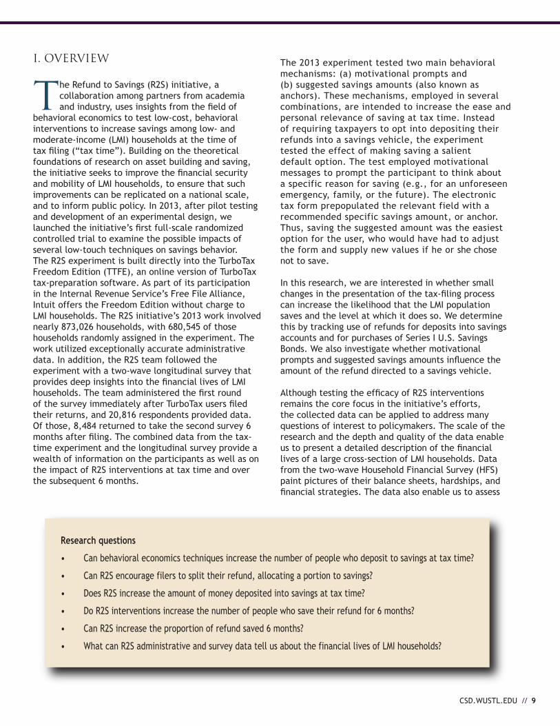
The 2013 experiment tested two main behavioral mechanisms: (a) motivational prompts and (b) suggested savings amounts (also known as anchors). These mechanisms, employed in several combinations, are intended to increase the ease and personal relevance of saving at tax time. Instead of requiring taxpayers to opt into depositing their refunds into a savings vehicle, the experiment tested the effect of making saving a salient default option. The test employed motivational messages to prompt the participant to think about a specific reason for saving (e.g., for an unforeseen emergency, family, or the future). The electronic tax form prepopulated the relevant field with a recommended specific savings amount, or anchor. Thus, saving the suggested amount was the easiest option for the user, who would have had to adjust the form and supply new values if he or she chose not to save.

In this research, we are interested in whether small changes in the presentation of the tax-filing process can increase the likelihood that the LMI population saves and the level at which it does so. We determine this by tracking use of refunds for deposits into savings accounts and for purchases of Series I U.S. Savings Bonds. We also investigate whether motivational prompts and suggested savings amounts influence the amount of the refund directed to a savings vehicle.

Although testing the efficacy of R2S interventions remains the core focus in the initiative’s efforts, the collected data can be applied to address many questions of interest to policymakers. The scale of the research and the depth and quality of the data enable us to present a detailed description of the financial lives of a large cross-section of LMI households. Data from the two-wave Household Financial Survey (HFS) paint pictures of their balance sheets, hardships, and financial strategies. The data also enable us to assess

I. OVERVIEw

The Refund to Savings (R2S) initiative, a collaboration among partners from academia and industry, uses insights from the field of

behavioral economics to test low-cost, behavioral interventions to increase savings among low- and moderate-income (LMI) households at the time of tax filing (“tax time”). Building on the theoretical foundations of research on asset building and saving, the initiative seeks to improve the financial security and mobility of LMI households, to ensure that such improvements can be replicated on a national scale, and to inform public policy. In 2013, after pilot testing and development of an experimental design, we launched the initiative’s first full-scale randomized controlled trial to examine the possible impacts of several low-touch techniques on savings behavior.

The R2S experiment is built directly into the TurboTax Freedom Edition (TTFE), an online version of TurboTax tax-preparation software. As part of its participation in the Internal Revenue Service’s Free File Alliance, Intuit offers the Freedom Edition without charge to LMI households. The R2S initiative’s 2013 work involved nearly 873,026 households, with 680,545 of those households randomly assigned in the experiment. The work utilized exceptionally accurate administrative data. In addition, the R2S team followed the experiment with a two-wave longitudinal survey that provides deep insights into the financial lives of LMI households. The team administered the first round of the survey immediately after TurboTax users filed their returns, and 20,816 respondents provided data. Of those, 8,484 returned to take the second survey 6 months after filing. The combined data from the tax-time experiment and the longitudinal survey provide a wealth of information on the participants as well as on the impact of R2S interventions at tax time and over the subsequent 6 months.

Research questions

• Can behavioral economics techniques increase the number of people who deposit to savings at tax time?

• Can R2S encourage filers to split their refund, allocating a portion to savings?

• Does R2S increase the amount of money deposited into savings at tax time?

• Do R2S interventions increase the number of people who save their refund for 6 months?

• Can R2S increase the proportion of refund saved 6 months?

• What can R2S administrative and survey data tell us about the financial lives of LMI households?

10 // WINTER 2015

whether the effects of the interventions persist over 6 months. They reveal perceptions concerning the burden of student-loan debt, the availability of health insurance, and trade-offs between short- and long-term financial gains. They also show how LMI households utilize tax refunds. Thus, the R2S data set could be a valuable tool in designing policy interventions to improve financial stability and mobility.

In the pages that follow, we begin by presenting a theoretical foundation for policies to promote financial security through asset building, and we specifically discuss the importance of tax time for increasing asset levels. We provide a detailed description of the R2S research design, data, and methods before presenting results from the experiment and the HFS. We conclude with a discussion of findings and consider implications for research as well as policy.

CSD.WUSTL.EDU // 11

II. BACkGROUND

ASSET BUILDINg AND IMPROVINg BALANCE SHEETS

Historically, public policies in the United States have been designed to improve the financial security of LMI households by offering a combination of income maintenance, consumption support, and work incentives. Although these policies help many households meet daily needs and manage finances, they have been less effective in addressing the lack of savings and in facilitating asset accumulation. Recent surveys find that over a quarter of Americans report having no emergency savings (Ross, 2014), and many are rendered financially vulnerable if unexpected or emergency spending needs arise (Chase, Gjertson, & Collins, 2011; Collins & Gjertson, 2013). A range of psychological, social, and institutional barriers prevent LMI households from setting aside funds to meet such needs. Disparities in financial literacy and education, the paucity of saving incentives, and inadequate access to financial institutions greatly limit the capacity to save (Beverly & Sherraden, 1999; Lusardi, 2008).

In recent years, proponents of asset-building policies have developed approaches to complement traditional policies for promoting the financial well-being of LMI households. These new approaches attempt to enhance the ability of those households to build savings and weather hardship (Sherraden, 1991). One such approach promotes saving at tax time.

WHy TAX TIME?

Tax filing is a nearly universal experience among Americans, and several important factors make tax time especially ideal for efforts to boost saving behavior. First, the tax refund is the largest lump sum that many households receive in a given year. In 2013 (returns for tax year 2012), the average tax refund was $2,755 per household (Internal Revenue Service, 2013a). That is a sizeable one-time windfall for many and a potential source of savings for LMI households. Results from the 2012 R2S Intention Survey support this notion: On average, participants reported the intention to save 40% of their refund (Key, Grinstein-Weiss, Tucker, Holub, & Ariely, 2013). Second, electronic filing options have altered the nature of the interaction with tax filers and enabled administration of low-touch, low-cost savings promotion interventions to millions of people. Eighty-three percent of tax returns are filed electronically, and around one third of electronically filed returns are self-prepared (Internal Revenue Service, 2013c). Third, the ability to receive tax refunds via direct deposit enhances opportunities for saving. The Internal Revenue Service

(2013c) distributed more than 79 million refunds via direct deposits into checking or savings accounts in 2013, and this number is substantially higher than the one from the previous year. Since 2006, the Internal Revenue Service has enabled filers to direct deposit refunds to multiple accounts by completing Form 8888. And since 2010, tax filers have been able to use the form to direct a portion of their refunds to purchase Series I U.S. Savings Bonds. Thus, the direct deposit mechanism and options on Form 8888 facilitate movement of refunds directly to savings vehicles. Fourth, opportunities for saving have arisen with the growth of the network of electronic filing platforms in the Internal Revenue Service’s Free File Alliance, which focuses on tax services for LMI households. These platforms present the opportunity to scale interventions so that they promote saving to millions of tax filers at relatively minimal cost. Incorporating effective savings promotions into tax-filing software may only require minor design changes, but the changes must be made thoughtfully. If these opportunities are harnessed, they have enormous potential to increase financial security among LMI households.

Recent evidence from other tax-time interventions affirms the importance of continuing to study such efforts. Tax-time interventions may facilitate interest in and utilization of savings accounts among LMI households (Beverly, Schneider, & Tufano, 2006; Beverly, Tescher, & Romich, 2004). They also may boost take-up of U.S. savings bonds (Tufano, 2011). In a study with tax filers in New York City who qualified for free tax preparation through the Volunteer Income Tax Assistance program, the $aveNyC program encouraged participants to deposit a portion of their tax refund into a savings account. To motivate saving, tax preparers offered monetary incentives to low-income participants who deposited a portion of their refund and did not withdraw any of the deposit for 1 year (Tucker, Key, & grinstein-Weiss, 2014).1 Around 70% of participating households saved their refunds for a full year, total savings amounted to $961,518 across all participants, and 72% continued to save after the program ended (UNC Center for Community Capital, 2013). Results from SaveUSA, the national version of the $aveNyC program, also show that most participating households saved for the full year and received a savings match (Azurdia, Freedman, Hamilton, & Schultz, 2013). Two similar incentivized-matching programs fielded through H & R Block successfully encouraged low-income tax filers to save a portion of their refund by contributing to an IRA account. In the 20% and 50% matching

1Preparers offered a 50% match to eligible participants: For every dollar of the refund held over 1 year, the $aveNyC study paid a 50¢ match.

12 // WINTER 2015

conditions, average contributions to an IRA were four and seven times greater than contributions by participants in the no-match, control condition (Duflo, Gale, Liebman, Orszag, & Saez, 2005).

These and other tax-time interventions recognize taxpayers’ tendency to view tax refunds as financial windfalls (Shapiro & Slemrod, 2003). The tendency is based partly on people’s financial status relative to peers (Epley, Mak, & Idson, 2006) and influences consumption behavior in the United States during tax season (Chambers & Spencer, 2008). There also is a tendency to spend a windfall instead of saving it, and this may be a barrier that prevents many LMI filers from accumulating savings. However, interventions may reverse the tendency toward consumption if designed to help filers overcome psychological and behavioral barriers to saving.

THE NEED FOR SAVINgS

Asset-based interventions are driven by the perspective that financial security and well-being are determined by assets as well as by income (Grinstein-Weiss et al., 2012; Oliver & Shapiro, 2006; Shapiro, 2001; Sherraden, 1991). By saving for the future and accumulating contingency savings, a household can build financial security beyond the limits imposed by income and expenses. In LMI households, assets may also function as a protective factor, improve financial well-being, and serve as a means of economic and social development (Sherraden & Sherraden, 2000). Contrasted with households that have liquid assets (e.g., assets held in savings products), households that have no or few liquid assets are 2–3 times more likely to experience material hardship as a result of income instability, job loss, medical emergency, death of a relative, or other unexpected life event (McKernan, Ratcliffe, & Vinopal, 2009). Nonetheless, ownership of accounts that foster asset accumulation remains low among LMI households. Results from the 2012 R2S Intention Survey indicate that households with higher income are far more likely to hold asset-building accounts than LMI households are (Grinstein-Weiss, Tucker, Key, Holub, & Ariely, 2013).

Most Americans will experience economic insecurity at some point in their lives (Rank, 2005). Since the late 1960s, the risk of economic insecurity has been increasing for most Americans between the ages of 25 and 60 (Rank, Hirschl, & Foster, 2014). Across all levels of the income distribution, American households are unprepared for financial shocks (Grinstein-Weiss et al., 2013, Grinstein-Weiss, Russell, Tucker, & Comer, 2014). Many recognize the importance of emergency savings, but immediate needs and a lack of resources may limit the ability of some to set money aside (Brobeck,

2008). This dilemma is not surprising in the context of economic trends and particularly the recent economic downturn. Wages for LMI households have flagged since the 1960s (Gordon & Becker, 2008). In 2011, roughly 20% of all U.S. households lost nearly a quarter of their total resources (Hacker, 2012). The unemployment rate peaked at one in 10 in 2009, and though it has slowly improved (to about 7.6% at the time of this study), more than a third of the unemployed have been so for 6 months or longer (Bureau of Labor Statistics, 2014a, 2014b). The long-term unemployed face particular difficulty in reentering the job market (Krueger, Cramer, & Cho, 2014). These trends have contributed to the economically precarious situation of LMI households in the United States, and minority households have been disproportionately affected. A 2004 study found that 60% of households of color do not have the means to cover at least 75% of their monthly expenses, and the same is true in 40% of working-age households (Shapiro, Oliver, & Meschede, 2009). The likelihood of holding sufficient contingency savings is also correlated with factors like age, education, income, and marital status (Bhargava & Lown, 2006). Because of these factors, many households are vulnerable to the effects of unexpected loss of income and to necessary but unexpected expenses (financial shocks).

The experience of such financial shocks varies across households. Financial emergencies are more common in and have a greater impact on larger households. Expenses and child-rearing costs rise with household size. Also, households with more children have less emergency savings and are less likely to be prepared for unexpected expenses (Babiarz & Robb, 2014). Average annual expenditures per child range from $8,990 to $10,230 among LMI families (Lino, 2013), and a financial shock may significantly interfere with a family’s ability to meet these costs. Accordingly, households with children report difficulty coping with financial shocks, and the severity of such shocks is associated with the number of children (Lusardi, Schneider, & Tufano, 2011). Thus, encouraging families to save may be especially important and challenging.

A financial emergency can threaten an unprepared household’s economic, social, psychological, and physical well-being. When presented with a financial shock, many households seek out alternative financial services such as those offered by payday lenders, pawn shops, and check-cashing outlets. The services tend to be predatory and financially harmful. They typically charge exorbitant interest rates and fees, placing households in a difficult, long-term struggle to repay the obligation. These services and products often limit long-term savings, purchases of necessities, and access to credit and other financial institutions (Barr, 2012; Chase et al., 2011; Couch, Daly, & Gardiner, 2011;

CSD.WUSTL.EDU // 13

Heflin, London, & Scott, 2011; Rawlings & Gentsch, 2008).

Many people who encounter a financial shock and lack contingency resources experience psychological distress. Such distress can reduce the quantity and quality of interactions with members of their household (Rothwell & Han, 2010), negatively affect children and marriages, and lead to adverse effects on physical and mental health (Conger et al., 2002; Finke & Pierce, 2006). Likewise, lack of adequate funds during a financial crisis may limit access to material necessities and result in material hardship, which can negatively affect health and well-being (Pilkauskas, Currie, & Garfinkel, 2012). Families coping with such events often forgo medical care or are unable to cover the costs of food, housing, and clothing (Beverly, 2001; Heflin et al., 2011). Having savings may reduce the incidence and impact of material hardship. Families that use banking services and own bank accounts are far less likely to experience material hardship than are unbanked and underbanked families (Lim, Livermore, & Davis, 2010). However, the lack of access to or engagement with a banking institution is an important barrier to saving, and it prevents many LMI households from accumulating assets.

PSyCHOLOgICAL AND BEHAVIORAL FACTORS

Recent evidence from behavioral economics provides a framework for understanding and promoting positive financial behaviors. Policymakers are leveraging this research to develop approaches that can increase economic security (Amir et al., 2005). As such research shows, people are not the rational economic actors that traditional, neoclassical economics would suggest them to be (Ariely, 2010, 2011; Becker, 1976; Caplan, 2000; De Bondt & Thaler, 1994; Kahneman, 2003; Kahneman & Tversky, 1979; List, 2004). Their everyday economic behaviors (i.e., saving, buying, and consuming) are predictably uncalculated and driven by psychological, social, and emotional processes. Furthermore, procrastination, inertia, and limited attention limit sound financial decision making (Johnson et al., 2012).

Such insights into cognitive biases have led proponents of asset building to develop strategies to encourage positive financial choices. Taking into account human irrationality allows us to adapt the ways in which information is presented and to consider which conditions will encourage individuals to override faulty perceptions. In other words, techniques based in behavioral economics have the potential to remove psychological and behavioral barriers to saving at tax time (Congdon, Kling, & Mullainathan, 2009). Several

lessons from behavioral-economics studies may be applied to interventions that encourage people to save.

Future orientation

Typically, individuals make decisions grounded in the present, but they discount the future (Benhabib, Bisin, & Schotter, 2010). Research on this present bias can explain why many do not save enough for retirement (Diamond & Köszegi, 2003). Interventions aimed at shifting the orientation of decision makers to the future show promise as pathways to encouraging long-term savings (Bryan & Hershfield, 2012; Hershfield, et al., 2011). A related phenomenon is the tendency to assume that one’s financial, personal, and social position will be better in the future (Bryan & Hershfield, 2012). People may discount the likelihood of emergency events, including auto or home repairs, moving expenses, and health-related costs. These tendencies limit the likelihood of planning for such unforeseen events.

Findings from the 2012 R2S Intention Survey suggest ways to minimize present bias. For example, the survey prompted treatment participants to think about their future selves at retirement and asked them to register their intentions concerning the allocation of their tax refund. Among those with an annual adjusted gross income less than $35,000, treatment participants intended to allocate 13% more of their tax refunds to savings than control participants did (Key et al., 2013).

Choice architecture

Individuals are constantly presented with choices. By employing choice architecture—design features created to increase the salience and perceived attractiveness of a given financial choice—researchers can help people avoid common pitfalls in decision making (Johnson et al., 2012). In the process, researchers increase the likelihood that consumers will choose to improve their economic well-being or decrease the likelihood of that they will behave in a financially detrimental manner. For example, choice architecture might limit the number of possible choices so that the only options are financially beneficial ones. Such techniques have been used effectively in Medicare drug plans (Congdon, Kling, & Mullainathan, 2011) and investment plans (Cronqvist & Thaler, 2004).

The power of the default option

In many situations, people tend to rely on the default options given to them (Kahneman, 1991). This reliance

14 // WINTER 2015

can stem from inertia or from their comfort in and trust of the status quo. Promising results have emerged from behavioral-economics interventions that leverage this tendency toward the default. Interventions to boost retirement savings show that making enrollment the default option (instead of requiring one to act in order to enroll) can increase utilization of savings products and might increase long-term commitment to saving (Benartzi & Thaler, 2007; Beshears, Choi, Laibson, & Madrian, 2009; Choi, Laibson, Madrian, & Metrick, 2004).

Anchoring

Informational markers or points of reference influence decisions involving the selection of a value, and this phenomenon is known as anchoring (Munro & Sugden, 2003; Sen, 1993). Research shows that individuals generate their own anchors and tend to choose values close to the initial values considered (Epley & Gilovich, 2001, 2004, 2005; Tamir & Mitchell, 2012). Self-generated reference points are vulnerable to faulty human perception because individuals rely on missing or incomplete information to create them (Epley & gilovich, 2006). However, people have a tendency to stay on or near anchors if such reference points are provided (Simmons, LeBoeuf, & Nelson, 2010). A potential strategy to increase the amount of savings is to provide such anchors (for example, if we suggest saving 75% of the refund, we would expect filers to choose to save close to 75% of their refunds).

In summary, research demonstrates the need for emergency savings and the potential benefits of such savings for LMI households. Electronic filing programs create a special opportunity to encourage and facilitate saving at a time when millions of Americans receive a substantial sum of money. Incorporating several established principles from behavioral economics may enhance strategies to boost saving. This context has influenced the design of the R2S study and the findings detailed in this report.

CSD.WUSTL.EDU // 15

III. RESEARCh DESIGNThe R2S initiative is a large-scale, multiyear research project that tests the impact of interventions on saving behaviors at tax time. Designed as a randomized controlled trial, the experiment randomly assigned tax filers to one of several treatment conditions informed by behavioral economics or to a control condition with no exposure to an intervention. The use of randomization and a control group, design features that are widely accepted as benchmarks in clinical and field research, enable us to compare treatment conditions and isolate treatment effects. We expect that the different groups would have the same average outcomes if they were not exposed to the treatments and that we can attribute any differences between groups to the effect of the intervention.

PARTICIPANTS

As part of its participation in the Free File Alliance, Intuit offers the free online TTFE to filers who meet certain criteria. In 2013, tax filers were qualified to use TTFE if they (a) had an adjusted gross income of less than $31,000, (b) qualified for the Earned Income Tax Credit (EITC), or (c) were an active-duty member of the military with an adjusted gross income of less than $57,000. The TTFE platform enables testing of interventions with a large, nationwide participant pool.

The experiment launched on January 31, 2013, the second day of the 2013 tax-filing season, and closed 2 days after the tax-filing deadline: April 17, 2013.2 To test many different interventions, we split the tax-filing season into three test periods: 259,429 filers participated during Period 1 (January 31–February 13), 207,215 participated during Period 2 (February 14–March 13), and 213,901 participated during Period 3 (March 14–April 17). In each subperiod, TTFE assigned all users receiving a tax refund to a control group or to one of six treatment conditions, and the probability that a participant would be assigned to a given group was equal across the groups.3 The sample for the 2013 R2S experiment consists of 680,545 LMI tax filers who submitted returns through TTFE and whose returns indicated that they were due a refund.

2Software developments necessary for the R2S experi-ment were not ready to deploy until January 31, 2013; Filers who began preparing their taxes on or before January 30 (n = 95,857) were unable to participate.

3Because they could not be assigned randomly to a treatment condition, we excluded tax filers who start-ed the filing process in a different TurboTax product and later used TTFE (n = 91,383).

INTERVENTION

The experiment tested two behavioral mechanisms: motivational messages (i.e., prompts) and default suggestions for the amount to be saved (i.e., anchors). The 2013 prompts reflect lessons learned during previous phases of the initiative (Grinstein-Weiss, et al., 2013; grinstein-Weiss, gale, et al., 2014; Key, et al., 2013). The TTFE software presented prompts to filers near the end of the tax-filing experience, after they learned the amount of their refunds. Each prompt appeared at the top of the web page, beside a small graphic depicting a piggy bank. The experiment included three treatment prompts and one comparison prompt:

Emergency prompt: “Do you have enough money for an emergency? A Harvard study found that most Americans could not come up with $2,000 for something unexpected. We can help you stay prepared.”

Family prompt: “Have a family or thinking of starting one? Start building a bright future for them.”

Future prompt: “Save for your future, and get peace of mind. Feel more secure about your future with a little extra money in the bank.”

Generic prompt: “Why not save a little money? you can split your federal refund into a savings account or get a U.S. Series 1 Savings Bond.”

Any effects of the treatment messages are relative to that of the Generic message (akin to treatment as usual), which also prompted tax filers to save. The treatment prompts differ from the generic prompt in that we integrated behavioral economics principles into their designs. Thus, importantly, any superiority of a treatment prompt over the control prompt is attributable to the implementation of behavioral economics techniques—not simply to the prompting to save. All three treatment messages prompt filers to consider a concrete reason for saving. Although the Future prompt is the most explicit of the three, all treatment messages prompt filers to consider the future. The Emergency message differs from the other treatment prompts in that it includes a social proof (Cialdini, 2006). The behavioral principle of social proof is included by prompting filers to think about how their situations compare with those of “most Americans.”

Anchoring, the other major behavioral mechanism tested in R2S, involves recommending a savings level to participants in treatment groups and prepopulating a field in the web form with that amount or percentage. The 2013 R2S experiment employed five anchors:

16 // WINTER 2015

1. 25% of the tax refund



4. $100

5. $250

The TTFE software presented a randomly assigned anchor to each refund recipient in one of the six treatment groups within each test period. Refund recipients in the control condition received no anchor. As Figure 1 shows, TTFE presented the anchors directly below the prompt, and the prompt was set in green font so that it would stand out from the other text on the page. Filers assigned to treatment groups with dollar-amount anchors (i.e., $100 or $250) did not see a suggestion to save a percentage of the refund.

Because savings bonds are available only in multiples of $50, TTFE rounded down the prepopulated savings amounts to the nearest $50. For example, a filer who was due a refund of $450 and assigned to a treatment

group with a 50% anchor saw a suggested savings amount of $200: the amount remaining after 50% of the refund ($225) is rounded down to the nearest increment of $50.4 Because rounding has a proportionally greater effect on anchors for small refunds, analyses generally exclude participants with refunds of less than $250 (n = 82,352). Interventions consisted of different combinations of prompts and anchors (see Table 1). The interventions consisted of a single screen, which was integrated with essential functions of tax-filing software and which users could easily navigate in seconds or minutes.

DATA COLLECTION

TurboTax software data

Intuit created a completely anonymous set of data on all TTFE users receiving a refund and shared this

4With rounding, the suggested amount is actually equiva-lent to 44% of the $450 refund in the example. On aver-age, the nominal anchor was 3.3% less than the actual one. Most tax filers (79%) saw a nominal anchor that was within 5% of the actual one.

Figure 1. A screenshot within TurboTax Freedom Edition showing an Emergency prompt paired with a prepopulated savings sug-gestion anchored at 25% of the tax refund.

CSD.WUSTL.EDU // 17

with the researchers for analysis. These TTFE data provide filing status (e.g., single or married and filing jointly), the number of dependents, age, income, tax credits and deductions claimed, and the amount of refund received. Because the data came directly from federal income tax returns, and there are potential financial or legal consequences for inaccurate filings, we assume they are highly accurate. The data set also indicates treatment status (assignment to the control group or to one of the treatments) and includes a measure of the outcome of highest interest: allocation of the refund. A filer could choose to receive the refund via electronic deposit or as a paper check. The entire refund could be sent to a single account (e.g., checking account) or divided (e.g., between checking and savings accounts, or between a paper check and Series I U.S. Savings Bond).5 The TTFE data capture (a) whether the participant deposited any of the refund into a savings vehicle (a savings account or savings bond); (b) whether the participant split the tax refund, allocating at least part of it to a savings vehicle; and (c) the portion—in dollars and as a percentage of the total refund—directed to a savings vehicle.

Longitudinal survey data

We supplemented TTFE data with information from two waves of the HFS, which enabled us to assess the impact of the R2S interventions over a 6-month period and to collect detailed information about the financial lives of LMI households. A link within TTFE invited experiment participants to complete the first wave of the survey (HFS1) immediately after they filed their taxes. We designed the HFS1 to take approximately

5Internal Revenue Service Form 8888 underlies the op-tion in the TTFE platform to split the refund across more than one account or vehicle.

20 minutes and allowed participants to skip questions. We collected the survey data via Qualtrics online software, obtained explicit consent from participants (pursuant to Title 26, Section 7216, of the Internal Revenue Code), and paired the data from the survey with that from the TTFE software.

We invited TTFE users to take the HFS1 if they filed a return on or after January 31 and received a federal tax refund. About half of the HFS1 questions focused on debts and assets. The responses provide information for household-level variables rather than for individual-level ones. The survey asked respondents to report whether their households have specific types of debts and assets (see Tables 7 and 8). It also asked them to estimate the value of those obligations and holdings. If respondents did not answer the valuation question, a follow-up question asked them to choose from a list of value categories (i.e., $0, Less than $500, $501–$1,000, $1,001–$2,000, more than $2,000). Other survey sections focused on filers’ financial behaviors, such as budgeting strategies and the use of alternative financial services (e.g., payday loans), during the 12 months prior to the survey. Many HFS1 questions directly replicated previously validated survey instruments. For example, we drew upon the work of Lusardi et al. (2011, p. 88) for the following question: “How confident are you that you could come up with $2,000 if an unexpected need arose within the next month?”

In the HFS1 data set, one area of high interest is the information on intended use of tax refunds. The survey asked respondents about their plans for their refunds and instructed them to specify the expected allocation of the refund by giving the percentage earmarked for each of the following categories:

1. “Paying off debt you owe now”

2. “Spending in the next month or so on products, services, or regular bills like rent or utilities”

Period 1 (January 31–February 13) Period 2 (February 14–March 13) Period 3 (March 14–April 17)

Generic, no anchor (control) Generic, no anchor (control) Generic, no anchor (control)generic, 25% generic, 50% Emergency, $100

generic, 50% generic, 75% Emergency, $250

Emergency, 25% Emergency, 50% Future, $100

Emergency, 50% Emergency, 75% Future, $250

Future, 25% Future, 75% Emergency, 25%

Family, 25% Family, 75% Future, 25%

Note: Generic, Emergency, Future, and Family indicate the prompts presented to filers via the in-product offer in TurboTax Freedom Edition. The percentages and dollar amounts indicate the suggested anchors.

Table 1. Combinations of Prompts and Anchors Tested in the Refund to Savings Experiment over Three Test Periods

18 // WINTER 2015

3. “Savings you expect to keep for a few months”

4. “Savings you expect to have this time next year”

5. “Savings for something further in the future”

To gather information about their actual use of the tax refunds, we subsequently e-mailed HFS1 respondents, inviting them to participate in a follow-up survey (HFS2) conducted 6 months after tax filing. To observe changes over time, the follow-up survey posed the same questions asked during the HFS1, but we added several items to capture household financial situations during those 6 months. In addition to the questions from HFS1, the HFS2 asked respondents whether they moved, started a new job, or experienced any of several financial shocks: A household member experienced a period of unemployment, required a trip to the hospital, needed a major vehicle repair, or paid legal fees. The HFS2 also asked respondents what they did with their tax refunds. The allocation categories differ from those used in HFS1, and saving is collapsed into one category. Respondents to the HFS2 indicated the percentage of the refund allocated for each of the following purposes:

1. “Used to pay down debt”

2. “Spent within 1 month of receiving the refund”

3. “Spent after 1 month of receiving the refund”

4. “Saved and still have”

We followed this survey item with more specific questions about use of refunds. For example, we asked those who paid down debt to specify the types of debt they paid. Similarly, we asked those who spent part of their refund to identify the kinds of items purchased, and we included an open-ended “other” category. We also asked those who saved their refund what kind of accounts they saved in, and we offered the following response options: regular savings account, checking account, prepaid card, retirement account, education account, U.S. savings bonds, or other (the respondent could specify). Those who reported saving any portion of their refunds for 6 months were also asked what they saved for: emergencies or other unexpected needs, a special purchase, retirement or other long-term needs, children or grandchildren, or other.

An important element of the HFS2 is that it allows participants to define saving: The survey asked them to specify the percentage of the refund saved, regardless of where they saved it (e.g., holding refund money as cash or in a checking account). In contrast, the TTFE data use a more limited definition: Saving is a deposit into a savings account or a purchase of savings bonds as opposed to

receipt of a mailed paper check or deposit into a checking account. One implication is that some participants identified as savers in HFS2 were not classified as savers according to the definition used in the TTFE data. As such, HFS2 provides a more accurate and complete picture of respondents’ actual tax-refund saving behaviors, which may have been influenced by prompts and anchors even if respondents did not choose to deposit their refunds into a savings account or to purchase savings bonds at tax time. The limited definition of saving in the TTFE data also may mean that the measured effects of the interventions understate the true impact. Conversely, the TTFE data may mistakenly identify participants as savers if they deposited the refund into savings at tax time but then transferred the money for other purposes. Data from HFS2 enable us to explore these possibilities.

We identified two main outcome measures of interest from the HFS2: whether participants saved any of their refunds for 6 months and the amount saved. We are interested in whether these outcomes differ by randomly assigned treatment conditions.

One caveat is that HFS data were self-reported, and the survey included several questions that may have been difficult to answer accurately. However, a comparison of data from the TTFE and the two waves of the HFS suggests that the self-reported HFS responses are highly reliable. For example, even 6 months after filing their taxes, respondents’ self-reports of tax refund amounts correlated with the refund amounts in the TTFE data (r = .95, p < .001).

We cannot determine how accurately responses reflect reality. Unless participants kept tax-refund savings separate

Summary of savings outcome measures

TTFE data: Tax-time savings deposits

• Whether filers deposited any of the taxrefund to a savings vehicle

• Whether filers split the tax refund to asavings vehicle

• Dollar amounts deposited to a savingsvehicle

HFS2 data: 6-month savings

• Whether survey respondents reported that they “saved, and still have” anyrefund (note: not necessarily in savingsvehicle)

• Percentage of the refund that theyreported they “saved, and still have”

CSD.WUSTL.EDU // 19

from other savings and income, they may have been unable to determine at the HFS2 how much of the refunds they used for spending, saving, and debt repayment. Therefore, we consider the response to the question about the saved amount to be largely perceptual.

We also can examine measures of holdings (i.e., assets and liabilities, and calculated liquid assets and net worth) and changes over time, but we observed large, unexpected fluctuations between the time of filing and the HFS2. As such, we focus on the self-reported use of tax refunds.

ANALySIS

Analysis of TTFE data is relatively straightforward: We can largely ignore issues related to selection bias and mitigating financial factors, because there was no opportunity for self-selection into the R2S experiment, and financial factors are equally distributed across groups via randomization. We also can be confident that the outcomes observed among treatment groups resulted from the exposure of those groups to the respective treatments. Descriptive comparisons of treatment-group characteristics confirm that the random assignment effectively generated roughly equivalent groups. Simple t-tests are sufficient to compare outcome means and proportions among treatment groups. In general, we believe that findings from TTFE data can be generalized to the LMI taxpayer population in the United States; however, we recognize that the sample may disproportionately represent individuals who file their own taxes and are Internet savvy.

Variation in tax filers’ characteristics by the timing of filing (i.e., when they filed during the tax season) complicates analysis. For example, people who file early in the tax season have significantly larger refunds, claim more dependents, and are more likely to file as head of household. Thus, we cannot compare outcomes of interventions across test periods without controlling for filing date.

Because we cannot assume that HFS respondents are selected randomly, analysis of HFS data—especially data from the HFS2—required a different empirical approach than the one employed in analysis of the TTFE data. Respondents to the two waves of the HFS differ from the TTFE population in several observable ways. For example, HFS respondents are somewhat older and more likely to be married. Of greater concern is the possibility that unobserved factors influence the likelihood of participating in the HFS. As a result, we generally refrain from using HFS data to make assumptions about the TTFE population. However, we compared participants within each test period and observed no differences in HFS response rates across treatment conditions. We therefore

can confidently measure treatment effects within the HFS subsample.

The HFS subsample is considerably smaller than the TTFE population. To maximize the sizes of comparison groups, we combined interventions with the same prompt or anchor in some models, rather than examining each specific intervention combination. For example, some models estimated the influence of anchor levels on savings outcomes but disregarded prompts. Others estimated the effects of the different prompts but ignored the anchor level. Findings from analysis of the 2012 TTFE data reveal that anchors are more effective than prompts in increasing the amounts of deposits to savings vehicles and that prompts are not associated with savings differences (Grinstein-Weiss, Gale, et al., 2014). Because we identified the anchor as the main mechanism for determining the level of tax-time saving, we can restrict HFS2 data analyses to focus on examining the marginal effects of anchor levels on saving behaviors in the 6 months between filing and the HFS2.

We used multiple regression techniques to control for many factors that may affect outcomes and to improve overall model fit; we selected these covariates on a model-by-model basis. We generally incorporated factors that may explain saving behaviors after tax time. Most models accounted for participant’s age, number of dependents, and tax refund amounts. When we analyzed data from the entire experiment’s sample, rather than from respondents who filed during a single test period, we included the filing date as a covariate. Sample sizes vary slightly from one analysis to another because of listwise exclusion of cases when data are missing. Because anchors were rounded down to the nearest $50 increment, we also employed a covariate to account for the difference between the nominal and actual anchors. In models that estimated the effects of anchors, we used this covariate to account for the potential downward bias of instances in which the actual and nominal anchors differ. If level of debt or assets was the outcome of interest, we included other predictors (e.g., level of education and race).

We based regression models on the outcome of interest. We employed ordinary least squares regression to estimate continuous outcome variables (e.g., the amount deposited into a savings account) and logistic regression to estimate binary outcome variables (e.g., whether a participant saved any of the refund).

20 // WINTER 2015

Imm

edia

tely

af

ter f

iling

taxe

sTa

x tim

e6

mon

ths

late

r

All TurboTax Freedom Editiontax filers who received a refund

Participated in HFS1 Included in descriptive analyses

Participated in HFS1Included in descriptive analyses

Participated in HFS2Sample for analysis of sustainedeffects of R2S

Included in descriptive analyses

Participated in HFS2Excluded from R2S analysis†

Included in descriptive analyses

Randomized in R2SViewed anchor-prompt combinationSample for analysis of tax-time effects of R2S

Not randomized*Excluded from R2S analysis

HFS1 total n = 20,816

HFS2 total n = 8,484

(n = 873,026)

(n = 680,545) (n = 192,481)

(n = 12,809) (n = 8,007)

(n = 4,940) (n = 3,544)

Figure 2. Overview of participant recruitment and inclusion in analyses. Note: R2S = Refund to Savings experiment; HFS1 = Household Financial Survey, first wave; HFS2 = Household Financial Survey, second wave.

*Those who submitted their taxes to the IRS before January 31, 2013, or who began filing in a different TurboTax product before using TurboTax Freedom Edition were not randomized.†The number of HFS participants excluded from the analysis of the R2S experiment includes those who were not randomized as well as those who may have been randomized but whose consenting names did not match the IRS record. The absence of a match between the consenting name and the record rendered their randomized assignment unknown to the researchers.

CSD.WUSTL.EDU // 21

IV. pARTICIpANT ChARACTERISTICSAs we have mentioned above, the 2013 R2S initiative involved data collected at three points: during TTFE filing, during the HFS1 immediately after tax filing, and during the HFS2 conducted 6 months later. During the TTFE phase of data collection, 873,026 individuals filed returns through the TTFE program and were due a tax refund. The analytical sample, which excludes individuals who were not randomly assigned to one of the experimental conditions, consists of 680,545 participants. For an overview of the acquisition of the analytical sample, see Figure 2. As Table 2 suggests, the analytical sample closely resembles the full population of 873,026 TTFE filers on most observed measures.

Most filers who contributed TTFE data (95%) qualified to use the free software by having an adjusted gross income of less than $31,000; however, 4.5% qualified by claiming the EITC (the adjusted gross income of these filers was higher than $31,000), and only 0.4% qualified through active-duty military service. It should be noted that the average income of TTFE filers receiving refunds (and that of R2S participants) was less than $15,000. That is significantly lower than the maximum income threshold ($31,000) specified in TTFE eligibility criteria. As Table 2 shows, the average age of TTFE filers was about 34 years. Roughly two thirds of participants filed with a household status of single, 21% filed as

head of household, and 10% filed jointly with their spouse as a married couple. Twenty-nine percent of participants in the TTFE data claimed a dependent on their tax return, and the average federal income-tax refund was $1,833 (see Illustration 1).

Assessed populationAnalytical Sample

(in R2S experiment)

Characteristic TTFE HFS1 HFS2 TTFE HFS1 HFS2

N 873,026 20,816 8,484 680,545 12,809 4,940

Age in years 34.1 36.1 35.2 34.0 36.4 35.5

(15.4) (14.1) (13.2) (15.7) (14.7) (13.8)

Gender (% female) NA 60.6 61.3 NA 58.9 59.8

Filing status

% single 66.1 63.5 63.9 68.4 68.3 69.7

% head of household 22.5 20.8 19.3 20.8 17.8 15.5

% married filing jointly 10.4 14.9 15.9 9.9 13.1 14.0

% current student NA 27.3 27.1 NA 28.2 27.8

% college educated NA 43.0 49.9 NA 43.2 51.0

% non-White race NA 21.3 20.2 NA 19.4 18.0

% Hispanic ethnicity NA 8.0 7.8 NA 8.2 8.1

% claiming dependents 31.6 33.3 33.0 29.1 28.1 26.9

Adjusted gross income ($) 14,819 16,546 17,520 14,378 15,666 16,634

(9,739) (10,208) (10,174) (9,600) (10,001) (9,968)

Federal tax refund ($) 1,964 2,105 2,179 1,833 1,835 1,875

(2,389) (2,305) (2,333) (2,332) (2,114) (2,117)

Note: IPO = in-product offer; HFS = Household Financial Survey; R2S = Refund to Savings experiment; TTFE = TurboTax Freedom Edition; HFS1 = Household Financial Survey, first wave; HFS2 = Household Financial Survey, second wave; NA = demographic characteristics are not collected with tax data. Unless otherwise specified, values are means with standard deviations in parentheses.

Table 2. Demographic Characteristics from the Experimental, Tax (TTFE), and HFS Data

Illustration 1. Characteristics of R2S participants. Values in top row are medians.

22 // WINTER 2015

After filing their taxes, 20,816 TTFE users responded to an invitation to take the HFS1. Of these, 18,839 (92%) could be matched to the TTFE data.6 A high proportion (91%) of people who began the HFS1 finished it. The entire survey took approximately 20 minutes to complete (20 minutes was the median). Overall, the demographic characteristics of the two HFS subsamples (participants who completed only HFS1 and those who completed both waves; see Table 2) are very similar to each other and to the full TTFE population. This indicates that selection bias is limited. For the first 3 days of the tax season, the R2S team offered filers a $20 incentive to take the HFS1. Thus, response rates to the survey were higher during that time (about 10% with the incentive vs. 1.2% without). We discontinued the incentive because the response exceeded our expectations and limited resources.

Six months after completing the HFS1, the R2S team invited 17,952 individuals to participate in the HFS2. Of those invited, 8,659 clicked the e-mailed link to take the survey (48% response rate), and 8,251 (95%) of those who responded to the invitation completed the HFS2. The average time elapsed between HFS1 and HFS2 was 6 months and 9 days (SD = 9 days). The response rate helps ensure that the HFS2 subsample is demographically comparable with the HFS1 subsample. Also, the experimental groups in the HFS2 did not differ within test period on any demographic characteristic. This indicates that group equivalence generated by randomization was retained and the ability to attribute differences to the intervention holds at the 6-month point. We offered a $20 incentive to those HFS2 participants who received an incentive for completing the HFS1 and $5 or $15 to HFS2 participants who received no previous incentive from R2S.

Compared with the subsample of filers who completed the HFS1, the HFS2 subsample was younger, had higher income, and reported higher educational attainment. The demographic traits of the two subsamples are otherwise very similar (see Table 2 for a summary of descriptive characteristics).

TAX-RELATED CHARACTERISTICS

Among TTFE filers receiving a refund, only 4% itemized their tax return; in comparison, about one third of all filers in the United States submit itemized returns

6 Names of survey participants granting consent were required to exactly match names on tax forms in or-der for Intuit to share the data with researchers at the Center for Social Development. For example, if a filer consented under a married surname but a maiden surname was on the tax record, the names would not match and data could not be shared.

(Internal Revenue Service, 2014b). About half of TTFE filers (54%) had no federal tax liability in 2012; the average tax liability among those with any was $918, and the median was $708. Most TTFE filers in this sample (93%) had taxes withheld via payroll deductions. The mean amount withheld was $1,122 in 2012, and the median was $758.

The EITC is an important policy that benefits many LMI filers; it is worth noting that 93% of refund-receiving TTFE filers reported earned income but that 59% did not qualify for the EITC. Our analysis of the TTFE data suggests that the EITC’s age requirements are the most common reason why filers without dependents were ineligible to receive the credit. A filer claiming no dependent was eligible to receive the EITC in 2013 if he or she was between the ages of 25 and 65 (Internal Revenue Service, 2013b). Among wage earners in the TTFE sample who did not receive the EITC (n = 477,398), 60% did not qualify because they were under age 25, and an additional 3% did not qualify because they were older than age 65. Income criteria excluded 23% of wage earners in this group.

The median EITC received by those who qualified was $2,142, and the mean was $2,191. Among TTFE filers who received any EITC, the credit makes up two thirds of the total federal tax refund. On average, the refund for those who received the EITC was more than 4.5 times higher than the refund for people who did not receive the credit ($882 vs. $3,498).

HOW DO R2S PARTICIPANTS COMPARE WITH THE U.S. POPULATION?

Perhaps because filing taxes online requires technical savvy, participants in the R2S experiment and the HFS tended to be younger and better educated than the general U.S. population. They also were more likely to be students. The median age of TTFE filers receiving a refund was 28 years in 2013, while the median age of U.S. taxpayers was about 45 (Internal Revenue Service, 2014b, pp. 77–78, Table 1.6). More than a quarter of HFS respondents indicated that they were enrolled students, but the rate of enrollment is only about 9% for the U.S. adult population.7 Compared with the general population of filers in the United States, HFS participants and TTFE users were also more likely to file as single and less likely to file as married filing jointly (Internal Revenue Service, 2014b). The racial makeup of HFS participants is similar to that of the

7 Estimated from the count of students enrolled in post-secondary institutions in 2012 (National Center for Ed-ucation Statistics, 2013) and from the total U.S. adult population in 2012 (U.S. Census Bureau, n.d.).

CSD.WUSTL.EDU // 23

general population in the United States: 21% of HFS participants identify themselves as non-White, and non-Whites comprise 22% of the U.S. population. Hispanic ethnicity is underrepresented in the HFS subsample: 8% of participants vs. 17% of the U.S. population (U.S. Census Bureau, 2013). In our study (TTFE data and HFS data), the proportion of households with dependents was about the same as the proportion of tax-filing households claiming dependents in the U.S. population (Internal Revenue Service, 2014a). Because use of TTFE is limited to filers who have low or moderate income, the median adjusted gross income of R2S participants was much lower than the U.S. median ($13,104 versus $36,055 for the U.S. population in 2012; Internal Revenue Service, 2014b, p. 27, Table 1.1). Similarly, the average tax refund of R2S participants ($1,833) was smaller than the U.S. average ($2,755) in 2013 (Internal Revenue Service, 2013a).

DIFFERENCES By FILINg DATE

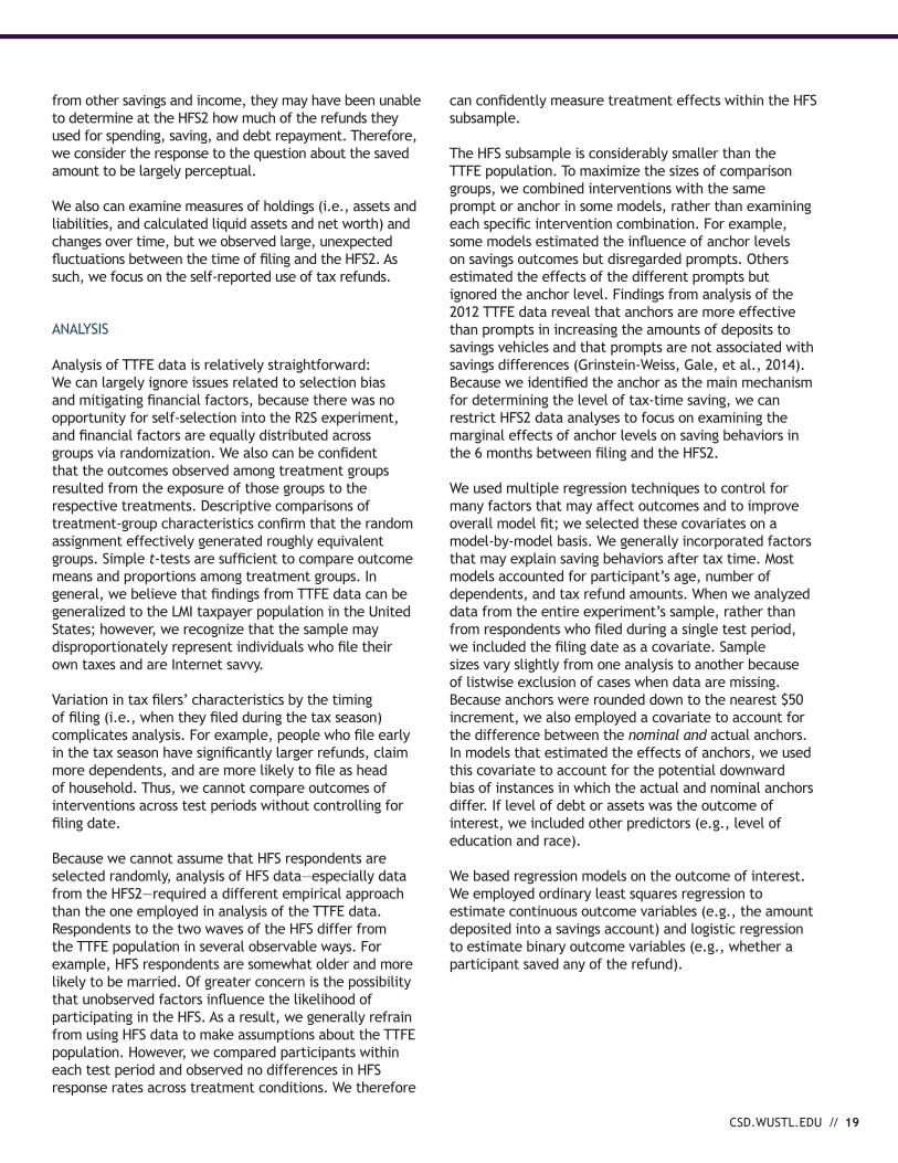
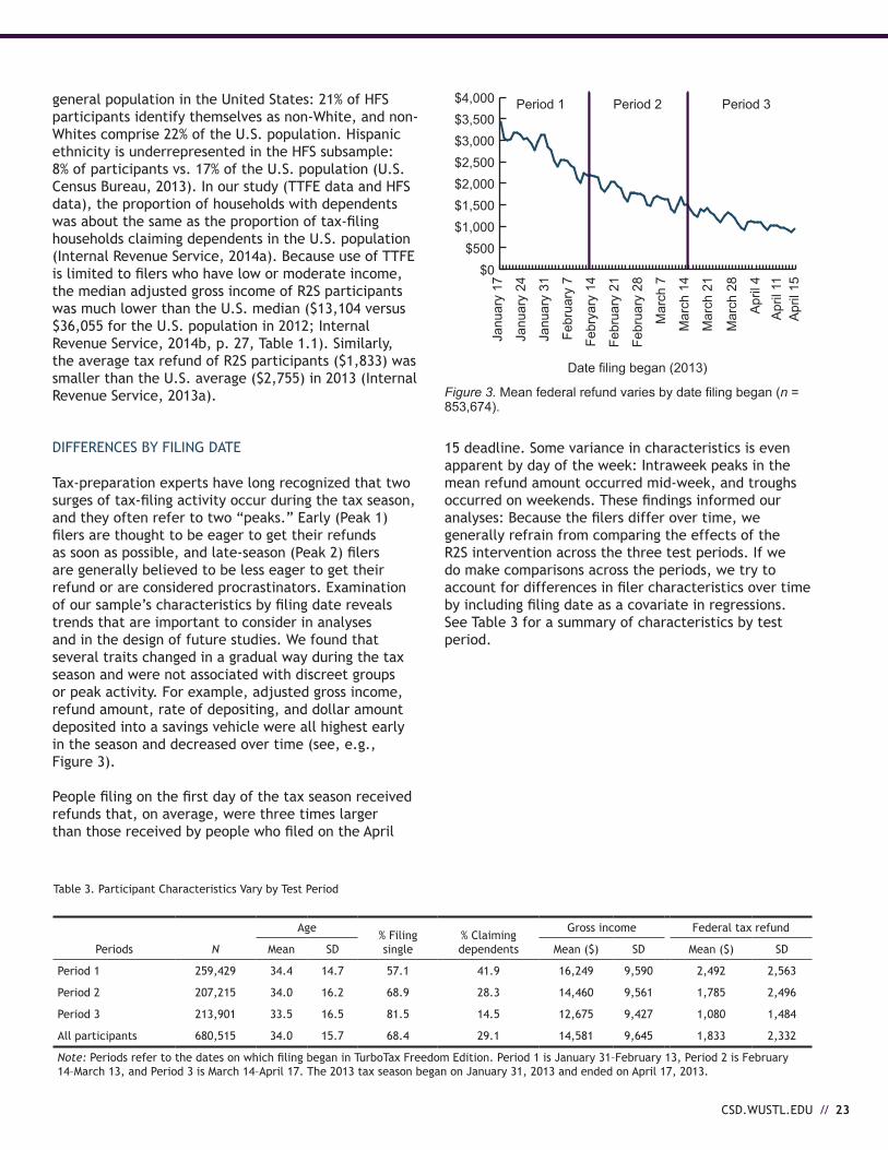
Tax-preparation experts have long recognized that two surges of tax-filing activity occur during the tax season, and they often refer to two “peaks.” Early (Peak 1) filers are thought to be eager to get their refunds as soon as possible, and late-season (Peak 2) filers are generally believed to be less eager to get their refund or are considered procrastinators. Examination of our sample’s characteristics by filing date reveals trends that are important to consider in analyses and in the design of future studies. We found that several traits changed in a gradual way during the tax season and were not associated with discreet groups or peak activity. For example, adjusted gross income, refund amount, rate of depositing, and dollar amount deposited into a savings vehicle were all highest early in the season and decreased over time (see, e.g., Figure 3).

People filing on the first day of the tax season received refunds that, on average, were three times larger than those received by people who filed on the April

$0$500

$1,000$1,500$2,000$2,500$3,000$3,500$4,000

Apr

il 15

Apr

il 11

Apr

il 4

Mar

ch 2

8

Mar

ch 2

1

Mar

ch 1

4

Mar

ch 7

Febr

uary

28

Febr

uary

21

Febr

yary

14

Febr

uary

7

Janu

ary

31

Janu

ary

24

Janu

ary

17

Period 1 Period 2 Period 3

Date filing began (2013)

Figure 3. Mean federal refund varies by date filing began (n = 853,674).

15 deadline. Some variance in characteristics is even apparent by day of the week: Intraweek peaks in the mean refund amount occurred mid-week, and troughs occurred on weekends. These findings informed our analyses: Because the filers differ over time, we generally refrain from comparing the effects of the R2S intervention across the three test periods. If we do make comparisons across the periods, we try to account for differences in filer characteristics over time by including filing date as a covariate in regressions. See Table 3 for a summary of characteristics by test period.

Age% Filing single

% Claiming dependents

gross income Federal tax refund

Periods N Mean SD Mean ($) SD Mean ($) SD

Period 1 259,429 34.4 14.7 57.1 41.9 16,249 9,590 2,492 2,563

Period 2 207,215 34.0 16.2 68.9 28.3 14,460 9,561 1,785 2,496

Period 3 213,901 33.5 16.5 81.5 14.5 12,675 9,427 1,080 1,484

All participants 680,515 34.0 15.7 68.4 29.1 14,581 9,645 1,833 2,332

Note: Periods refer to the dates on which filing began in TurboTax Freedom Edition. Period 1 is January 31–February 13, Period 2 is February 14–March 13, and Period 3 is March 14–April 17. The 2013 tax season began on January 31, 2013 and ended on April 17, 2013.

Table 3. Participant Characteristics Vary by Test Period

24 // WINTER 2015

CSD.WUSTL.EDU // 25

part Two

Research Findings: The Experiment

By employing a rigorous, randomized controlled design and principles of behavioral economics, the R2S experiment seeks to test interventions that encourage tax filers to save some of their refunds. In this section, we present results from the R2S experiment. Key outcomes include deposits to savings vehicles at tax time and participants’ uses of the tax refund in the subsequent 6 months.

26 // WINTER 2015

CSD.WUSTL.EDU // 27

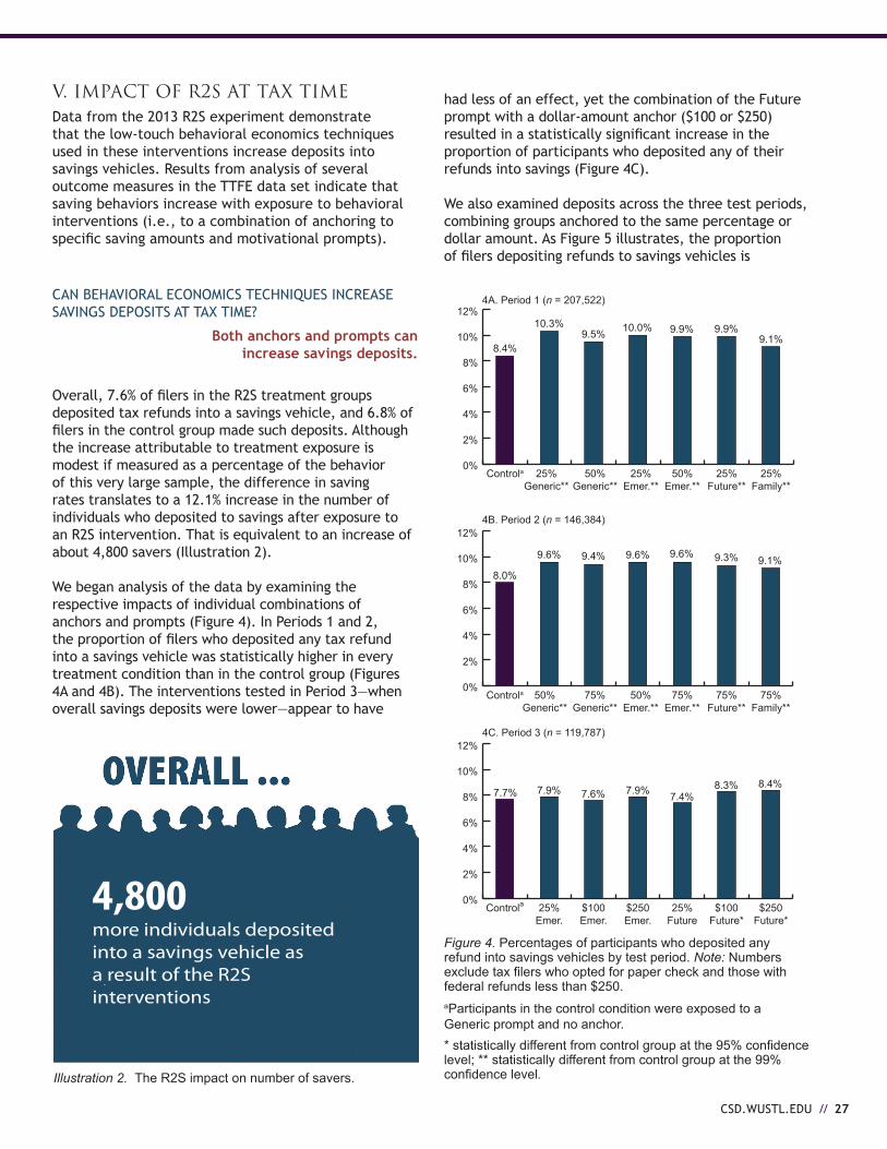
V. ImpACT OF R2S AT TAx TImEData from the 2013 R2S experiment demonstrate that the low-touch behavioral economics techniques used in these interventions increase deposits into savings vehicles. Results from analysis of several outcome measures in the TTFE data set indicate that saving behaviors increase with exposure to behavioral interventions (i.e., to a combination of anchoring to specific saving amounts and motivational prompts).

CAN BEHAVIORAL ECONOMICS TECHNIQUES INCREASE SAVINgS DEPOSITS AT TAX TIME?

Both anchors and prompts can increase savings deposits.

Overall, 7.6% of filers in the R2S treatment groups deposited tax refunds into a savings vehicle, and 6.8% of filers in the control group made such deposits. Although the increase attributable to treatment exposure is modest if measured as a percentage of the behavior of this very large sample, the difference in saving rates translates to a 12.1% increase in the number of individuals who deposited to savings after exposure to an R2S intervention. That is equivalent to an increase of about 4,800 savers (Illustration 2).

We began analysis of the data by examining the respective impacts of individual combinations of anchors and prompts (Figure 4). In Periods 1 and 2, the proportion of filers who deposited any tax refund into a savings vehicle was statistically higher in every treatment condition than in the control group (Figures 4A and 4B). The interventions tested in Period 3—when overall savings deposits were lower—appear to have

had less of an effect, yet the combination of the Future prompt with a dollar-amount anchor ($100 or $250) resulted in a statistically significant increase in the proportion of participants who deposited any of their refunds into savings (Figure 4C).

We also examined deposits across the three test periods, combining groups anchored to the same percentage or dollar amount. As Figure 5 illustrates, the proportion of filers depositing refunds to savings vehicles is

Figure 4. Percentages of participants who deposited any refund into savings vehicles by test period. Note: Numbers exclude tax filers who opted for paper check and those with federal refunds less than $250.aParticipants in the control condition were exposed to a Generic prompt and no anchor.* statistically different from control group at the 95% confidence level; ** statistically different from control group at the 99% confidence level.

4A. Period 1 (n = 207,522)

4C. Period 3 (n = 119,787)

4B. Period 2 (n = 146,384)

0%

2%

4%

6%

8%

10%

12%

25%Family**

25%Future**

50%Emer.**

25%Emer.**

50%Generic**

25%Generic**

Controla

0%

2%

4%

6%

8%

10%

12%

75%Family**

75%Future**

75%Emer.**

50%Emer.**

75%Generic**

50%Generic**

Controla

0%

2%

4%

6%

8%

10%

12%

$250Future*

$100Future*

25%Future

$250Emer.

$100Emer.

25%Emer.

Controla

8.4%

10.3%9.5% 10.0% 9.9% 9.9%

9.1%

8.0%

9.6% 9.4% 9.6% 9.6% 9.3%

7.7% 7.9% 7.6% 7.9% 7.4%8.3% 8.4%

9.1%

Illustration 2. The R2S impact on number of savers.

4,800more individuals depositedinto a savings vehicle as a result of the R2Sinterventions

28 // WINTER 2015

statistically higher if any anchor is present than if there is no anchor. Similarly, if participants are grouped across the three test periods according to the type of prompt, the proportion of filers who deposited some of their refund in a savings vehicle is greater among those who received the Emergency and Future prompts than among counterparts who received the generic prompt shown to members of the control group (Figure 6).

CAN R2S EFFECTIVELy ENCOURAgE PEOPLE TO SPLIT THEIR REFUNDS?

The interventions approximately double the rate of splitting.

Federal policy and electronic filing platforms enable taxpayers to split their refund by directing the treasury to disburse it to multiple accounts or savings vehicles. Our analysis shows that the intervention nearly doubles the

rate of refund splitting (including allocation to at least one savings vehicle): 0.86% of the control group and 1.55% of the treatment groups split their refunds to allocate some to a savings vehicle. Consistent with the results presented above, the effect of the interventions is stronger in the first two test periods than in Period 3 (Figures 7A-7C). Although refund splitting is uncommon in all conditions, the R2S interventions specifically prompted filers to split, and the observed increase in the targeted behavior suggests that low-touch techniques can influence tax-time choices as intended.

0%

2%

4%

6%

8%

10%

FamilyFuture*Emer.**Generic

8.8%9.2% 9.1% 8.8%

Figure 6. Probability of depositing any refund into savings vehicle at tax time by prompt message, based on regression estimates (n = 468,985). * statistically different from Generic prompt group at the 95% confidence level; ** statistically different from control group at the 99% confidence level.

Figure 7. Percentages of participants who split any refunds into savings vehicles by test period. Note: Numbers exclude tax filers who opted for paper check and those with federal refunds less than $250.aParticipants in the control condition were exposed to a Generic prompt and no anchor.* statistically different from control group at the 99% confidence level.

0.0%

0.5%

1.0%

1.5%

2.0%

2.5%

3.0%

25%Family*

25%Future*

50%Emer.*

25%Emer.*

50%Generic*

25%Generic

Controla

0.0%

0.5%

1.0%

1.5%

2.0%

2.5%

3.0%

75%Family*

75%Future*

75%Emer.*

50%Emer.*

75%Generic*

50%Generic*

Controla

0.0%

0.5%

1.0%

1.5%

2.0%

2.5%

3.0%

$250Future*

$100Future*

25%Future*

$250Emer.*

$100Emer.*

25%Emer.*

Controla

7A. Period 1 (n = 207,522)

7B. Period 2 (n = 146,384)

7C. Period 3 (n = 119,787)

1.4%

2.7%

2.3%2.6% 2.5% 2.6%

2.2%

1.1%

2.2% 2.2% 2.1% 2.1% 2.0%1.8%

0.8%

1.3% 1.4% 1.4%1.2% 1.3%

1.5%

Figure 5. Probability of depositing any refund into a savings vehicle at tax time by anchor amount, based on regression estimates (n = 468,947).* statistically different from no anchor group at the 99% confi-dence level.

0%

2%

4%

6%

8%

10%

$250anchor*

$100anchor*

75%anchor*

50%anchor*

25%anchor*

Control(No Anchor)

8.1%

9.1% 9.3% 9.3%8.7% 8.9%

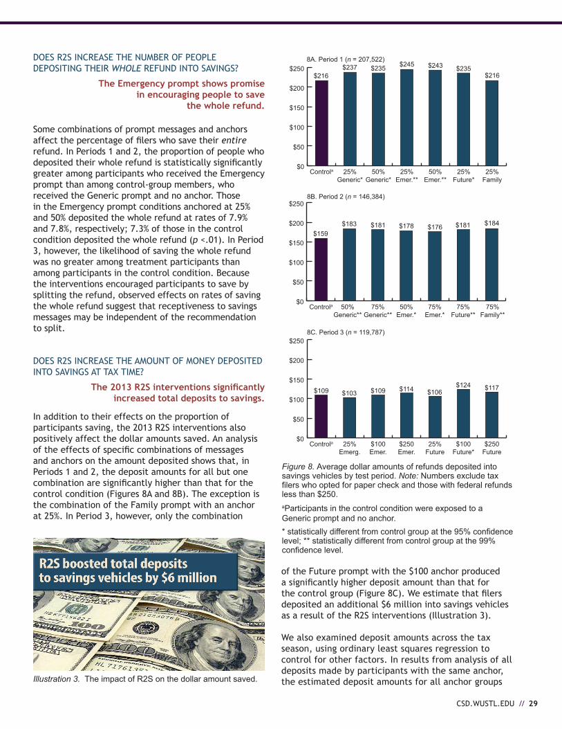
CSD.WUSTL.EDU // 29

of the Future prompt with the $100 anchor produced a significantly higher deposit amount than that for the control group (Figure 8C). We estimate that filers deposited an additional $6 million into savings vehicles as a result of the R2S interventions (Illustration 3).

We also examined deposit amounts across the tax season, using ordinary least squares regression to control for other factors. In results from analysis of all deposits made by participants with the same anchor, the estimated deposit amounts for all anchor groups

DOES R2S INCREASE THE NUMBER OF PEOPLE DEPOSITINg THEIR WHoLE REFUND INTO SAVINgS?

The Emergency prompt shows promise in encouraging people to save

the whole refund.

Some combinations of prompt messages and anchors affect the percentage of filers who save their entire refund. In Periods 1 and 2, the proportion of people who deposited their whole refund is statistically significantly greater among participants who received the Emergency prompt than among control-group members, who received the generic prompt and no anchor. Those in the Emergency prompt conditions anchored at 25% and 50% deposited the whole refund at rates of 7.9% and 7.8%, respectively; 7.3% of those in the control condition deposited the whole refund (p <.01). In Period 3, however, the likelihood of saving the whole refund was no greater among treatment participants than among participants in the control condition. Because the interventions encouraged participants to save by splitting the refund, observed effects on rates of saving the whole refund suggest that receptiveness to savings messages may be independent of the recommendation to split.

DOES R2S INCREASE THE AMOUNT OF MONEy DEPOSITED INTO SAVINgS AT TAX TIME?

The 2013 R2S interventions significantly increased total deposits to savings.

In addition to their effects on the proportion of participants saving, the 2013 R2S interventions also positively affect the dollar amounts saved. An analysis of the effects of specific combinations of messages and anchors on the amount deposited shows that, in Periods 1 and 2, the deposit amounts for all but one combination are significantly higher than that for the control condition (Figures 8A and 8B). The exception is the combination of the Family prompt with an anchor at 25%. In Period 3, however, only the combination

Illustration 3. The impact of R2S on the dollar amount saved.

Figure 8. Average dollar amounts of refunds deposited into savings vehicles by test period. Note: Numbers exclude tax filers who opted for paper check and those with federal refunds less than $250.aParticipants in the control condition were exposed to a Generic prompt and no anchor.* statistically different from control group at the 95% confidence level; ** statistically different from control group at the 99% confidence level.

$0

$50

$100

$150

$200

$250

25%Family

25%Future*

50%Emer.**

25%Emer.**

50%Generic*

25%Generic*

Controla

$0

$50

$100

$150

$200

$250

75%Family**

75%Future**

75%Emer.*

50%Emer.*

75%Generic**

50%Generic**

Controla

$0

$50

$100

$150

$200

$250

$250Future

$100Future*

25%Future

$250Emer.

$100Emer.

25%Emerg.

Controla

8A. Period 1 (n = 207,522)

8B. Period 2 (n = 146,384)

8C. Period 3 (n = 119,787)

$109 $103 $109 $114 $106$124 $117

$159$183 $181 $178 $176 $181 $184

$216$237 $235 $245 $243 $235

$216

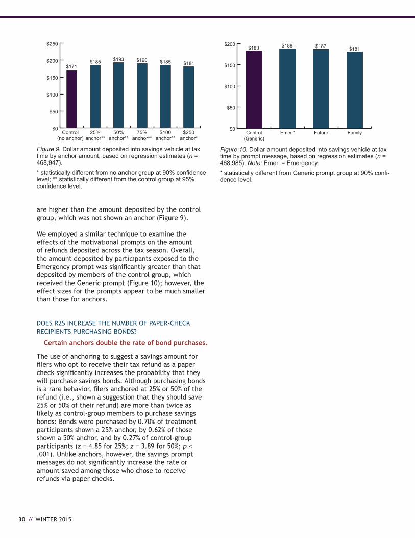
30 // WINTER 2015

are higher than the amount deposited by the control group, which was not shown an anchor (Figure 9).

We employed a similar technique to examine the effects of the motivational prompts on the amount of refunds deposited across the tax season. Overall, the amount deposited by participants exposed to the Emergency prompt was significantly greater than that deposited by members of the control group, which received the Generic prompt (Figure 10); however, the effect sizes for the prompts appear to be much smaller than those for anchors.

DOES R2S INCREASE THE NUMBER OF PAPER-CHECK RECIPIENTS PURCHASINg BONDS?

Certain anchors double the rate of bond purchases.

The use of anchoring to suggest a savings amount for filers who opt to receive their tax refund as a paper check significantly increases the probability that they will purchase savings bonds. Although purchasing bonds is a rare behavior, filers anchored at 25% or 50% of the refund (i.e., shown a suggestion that they should save 25% or 50% of their refund) are more than twice as likely as control-group members to purchase savings bonds: Bonds were purchased by 0.70% of treatment participants shown a 25% anchor, by 0.62% of those shown a 50% anchor, and by 0.27% of control-group participants (z = 4.85 for 25%; z = 3.89 for 50%; p < .001). Unlike anchors, however, the savings prompt messages do not significantly increase the rate or amount saved among those who chose to receive refunds via paper checks.

Figure 9. Dollar amount deposited into savings vehicle at tax time by anchor amount, based on regression estimates (n = 468,947). * statistically different from no anchor group at 90% confidence level; ** statistically different from the control group at 95% confidence level.

$0

$50

$100

$150

$200

$250

$250anchor*

$100anchor**

75%anchor**

50%anchor**

25%anchor**

Control(no anchor)

$171$185 $185$193 $190 $181

Figure 10. Dollar amount deposited into savings vehicle at tax time by prompt message, based on regression estimates (n = 468,985). Note: Emer. = Emergency. * statistically different from Generic prompt group at 90% confi-dence level.

$0

$50

$100

$150

$200

FamilyFutureEmer.*Control(Generic)

$183 $188 $187 $181

CSD.WUSTL.EDU // 31

VI. ThE ImpACT OF R2S 6 mONThS AFTER FIlING

Using data from the 6-month follow up (HFS2), we are able to test for sustained effects of the R2S interventions. The main outcome of interest here is not where the tax refund is deposited (a key concern in our analyses with the TTFE data) but rather whether the filer had any of that refund left after 6 months and, if so, how much remained. The primary outcome data come from a question about the percentage of the refund allocated for (a) spending within a month, (b) spending after 1 month but before 6 months, (c) debt payments, and (d) savings. In contrast with the relatively restricted measure of saving at tax time (defined by allocation of refunds at that point), the measure of saving in the HFS2 captures respondents’ perceptions of their own savings, which could include funds held in checking accounts, in cash, or in a traditional savings vehicle. This broad, respondent-determined definition of savings enables us to test of whether the R2S interventions influenced saving behavior and outcomes beyond the time of filing.

DOES R2S INCREASE THE NUMBER OF PEOPLE WHO SAVE THEIR REFUND FOR 6 MONTHS?

Higher anchors result in a greater chance of saving.

Figure 11 illustrates results from a logistic regression that examined the effects of the R2S interventions on the rate at which participants save refunds for 6 months. For this analysis, we collapsed groups with common anchor percentages or amounts, regardless of filing date. The results suggest that the likelihood of saving a portion of the refund for 6 months is significantly higher among filers shown the 50% anchor than among filers in the control group, which had

no anchor. The average control-group participant is estimated to have a 25.9% probability of reporting that he or she saved part of the refund for 6 months, yet treatment participants shown a 50% anchor are estimated to have a 30.6% probability of saving a portion for that time (p = .06). The probability is also about 30% among those assigned to a group shown a 75% anchor, although the standard error is larger for this group, and the difference from the control group is not statistically significant. Figure 12 illustrates results from a similar analysis conducted to evaluate the effects of prompts instead of anchors. If participants are grouped by prompt and not by filing date, the likelihood of saving a portion of the refund for 6 months does not significantly differ by treatment condition: Participants shown a treatment prompt are no more likely to save than are control-group participants, who received the generic message.

CAN R2S INCREASE THE PROPORTION OF THE REFUND STILL IN SAVINgS AFTER 6 MONTHS?

The 75% anchor increases the proportion in savings after 6 months.

To determine what proportion of refunds remained in savings at the HFS2, we estimated an ordinary least squares regression that controlled for several factors. The results suggest that, compared with participants in the control group, participants shown the 75% anchor saved a significantly greater proportion of their refunds for 6 months (Figure 13). Six months after filing, the control group still had slightly less than 15% of their refunds, but the group shown the 75% anchor had over 19%. The proportions saved by participants in groups shown other anchor levels do not differ significantly from those saved by the control group. We also estimated a regression that assessed whether the percentage of the refund remaining in savings varies by the prompt shown to participants, but we found no significant differences (Figure 14).

0%

5%

10%

15%

20%

25%

30%

35%

$250anchor

$100anchor

75%anchor

50%anchor*

25%anchor

Noanchor

24%24%

30%31%27%26%

Figure 11. Probability of saving refund for 6 months by anchor amount, based on regression estimates (n = 4,172). * statistically different from no anchor group at 90% confidence level.

0%

5%

10%

15%

20%

25%

30%

35%

FamilyFutureEmergencyGeneric

27%30% 30%

25%

Figure 12. Probability of saving for 6 months by prompt, based on regression estimates (n = 4,172).

32 // WINTER 2015

0%

5%

10%

15%

20%

25%

$250anchor

$100anchor

75%anchor*

50%anchor

25%anchor

Noanchor

% o

f ref

und

save

d fo

r 6 m

onth

s

15% 15%17%

19%

13% 14%

Figure 13. Percentage of refund saved for 6 months by anchor amount, based on regression estimates (n = 4,833). * statistically different from control group at 90% confidence level.

0%

5%

10%

15%

20%


% o

f ref

und

save

d fo

r 6 m

onth

s

15%17%

14%

17%

Figure 14. Percentage of refund saved for 6 months by prompt, based on regression estimates (n = 4,833).

DOES R2S AFFECT PERCEPTIONS OF THE ABILITy TO COME UP WITH $2,000?

Some interventions increase perceptions of access to emergency funds.

Our research suggests that R2S interventions also influence participants’ perceptions of their ability to access $2,000 in an emergency. At tax time (HFS1) and again 6 months later (HFS2), we asked whether the participant could “come up with $2,000 if an unexpected need arose within the next month” (Lusardi et al., 2011, p. 88). Respondents could select that they were certain they could, that they could probably, that they probably could not, or that they were certain they could not come up with $2,000. Figure 15 presents the predicted probability that a respondent certainly or probably could access $2,000. It shows estimated probabilities by anchor levels for each wave of the HFS. The results indicate that, at both points in time, participants shown a 50% or 75% anchor were significantly more likely than control-group members to answer affirmatively (p < .001). Those shown a $250 anchor were significantly more likely than control-group members to answer affirmatively at the 6-month follow-up survey (p < .05). One interesting takeaway from these data is that the increased confidence in access to emergency funds occurred at the time of filing, even before the tax refund would have been received. It is possible that the interventions primed participants to think about alternative sources of emergency funds. It is also possible that the interventions primed them to give a socially optimal answer but did not necessarily change the material conditions. It is interesting to note that the estimated changes in perceptions persisted for at least 6 months.

Figure 16 presents estimates from regressions predicting the probability of an affirmative response to the question on access to $2,000 for each wave of the HFS and for each prompt. Participants shown an Emergency prompt were more likely than control-group members to report at HFS1 that they had $2,000 for an emergency. Those shown a Family prompt were more likely than control-group counterparts to report this at HFS2. The statistically significant finding for the Emergency prompt is particularly interesting because the wording of the prompt specifically references the ability to come up with $2,000: “A Harvard study found that most Americans could not come up with $2,000 for something unexpected. We can help you stay prepared.” By explicitly referencing the $2,000 level and indicating that “most Americans” cannot access that amount, we may have prompted a psychological reaction rather than a behavioral one.

0%

10%

20%

30%

40%

50%

60%

HFS2HFS1

$250anchor

$100anchor

75%anchor

50%anchor

25%anchor

Noanchor

% o

f res

pond

ents

** **** **

*

Figure 15. Percentage of survey respondents who say they could come up with $2,000 in an emergency by anchor amount, based on regression estimates (n = 4,727). Note: HFS1 = Household Financial Survey, first wave; HFS2 = Household Financial Survey, second wave. * statistically different from control group at 95% confidence level; ** statistically different from no anchor group at 90% confidence level.

CSD.WUSTL.EDU // 33

SUMMARy OF RESULTS FROM THE 2013 R2S EXPERIMENT

In the 2013 R2S experiment, we evaluated the effectiveness of combining suggested savings amounts (anchors) with messages that were informed by the principles of behavioral economics, that prompted tax filers to split their tax refunds, and that encouraged them to allocate a portion into savings vehicles. To examine the effects of these interventions, we compared participants in carefully designed treatment conditions with counterparts in a control group, which we exposed to a generic savings-promotion message but not to an anchor. Our estimates show that exposure to the R2S interventions increased the number of savers, the number of people splitting the refund into savings, and the amount deposited into savings vehicles at tax time. However, the magnitude of effects on saving behavior varies by the timing of filing. In general, the magnitude of effects is greater among participants who filed in Period 1 or Period 2 than among those who filed in Period 3; however, the R2S team did not test the two high-percentage anchors (50% and 75%) in Period 3, so it is possible that other anchor–prompt combinations would have been more effective. In addition, data from the HFS provide evidence concerning the impact of the interventions over time. We estimate that high anchoring (50% or 75%) is associated with an increase in the probability of saving as well as with the percentage of the refund remaining in savings after 6 months. Observed long-term effects of minor design changes in the electronic filing software are noteworthy and hold promise for scalable impact on savings in LMI households.

0%

10%

20%

30%

40%

50%

60%

HFS2HFS1


% o

f res

pond

ents

* **

Figure 16. Percentage of respondents who say they could come up with $2,000 in an Emergency by prompt, based on regression estimates (n = 4,727). Note: HFS1 = Household Financial Survey, first wave; HFS2 = Household Financial Survey, second wave. * statistically different from the control group at 95% confidence level; ** statistically different from Generic prompt group at 90% confidence level.

34 // WINTER 2015

CSD.WUSTL.EDU // 35

part Three

Research Findings: Descriptive Results

Data from the TTFE software and HFS enable this research to extend beyond the research questions that this experiment set out to answer. These data offer an in-depth look at the preferences, behavior, and financial well-being of LMI households. In this section, we present valuable insights revealed by exploratory analyses. Particularly noteworthy are results from investigations of the roles that the characteristics of tax filers play in saving and the inability to save. For each topic, we present results from the largest sample available: In general, tax-related characteristics come from the entire available TTFE data set (i.e., all TTFE filers receiving refunds, including those not participating in the R2S experiment), characteristics assessed by survey come from the HFS1 subsample, and the HFS2 is the source for measures of events occurring in the 6-months following tax filing.

36 // WINTER 2015

CSD.WUSTL.EDU // 37

VII. RECEIpT AND UTIlIzATION OF TAx REFUNDS

In the TurboTax filing experience, after submitting all information relevant to income, credits, and deductions, filers owed a tax refund are shown options for receiving the refund. They may choose to receive refunds via direct deposit, paper check, or U.S. savings bonds. The user may opt to divide the tax refund between two bank accounts, between a bank account and a bond purchase, or between a paper check and a bond purchase. This end-of-filing experience is the setting for the R2S experiment, wherein we encourage filers to divide the tax refund and deposit a portion into a savings vehicle.

DIRECT DEPOSIT VERSUS PAPER CHECK

Filers with small refunds are more likely to opt for a paper check.

Most TTFE filers (83%) opt to receive at least part of their refund through direct deposit. In the TTFE data, refunds deposited into prepaid debit-card accounts are not distinguishable from those deposited into other types of accounts, but our analysis of data from the HFS1 shows that 2% of filers who chose direct deposit self-reported that they sent their refund deposit to a prepaid debit account. The TTFE data indicate that 17% of TTFE filers chose to receive at least part of their refund via a paper check sent in the mail.

Some evidence shows that filing date is tied to participants’ choices concerning refund payment. The probability of choosing a paper check increases as the filing deadline nears: 12% of filers chose to receive a paper check in Period 1, 17% chose this in Period 2, and 27% chose it in Period 3. We find additional evidence for this relationship in results from a logistic regression (results not shown), which also indicate that lacking a bank account, being unemployed, and lacking a college education are associated with the choice of a paper check. The odds of choosing a paper check decrease as gross income and federal tax-refund size increase. Furthermore, after adjusting for these variables, we found that the probability of choosing a paper check is significantly lower among females than among males and significantly lower among African Americans than among Whites.

Tax filers who wish to direct deposit may only deposit to existing accounts. Notably, however, 5.6% of HFS1 respondents reported having no checking or savings account. Encouraging the use of direct deposit and enabling filers to open bank accounts at the time of tax filing have the potential to speed up receipt of refunds, reduce the number of unbanked filers, foster engagement with financial institutions, and move funds directly into savings containers. The Internal Revenue Service has also expressed interest in decreasing the number of paper-check refunds because

direct deposit eliminates problems with lost, stolen, or undeliverable checks (Internal Revenue Service, 2008). Understanding the characteristics of people who are most likely to choose paper checks may inform strategies to boost use of direct deposit.

BONDS

Awareness of bonds is high, but usage is low.

Take-up of U.S. savings bonds was low at tax time: Only 0.3% of TTFE filers (n = 2,937) purchased bonds with their refunds. The HFS2 asked participants: “Are you familiar with U.S. savings bonds?” Fifty-eight percent of respondents said, “Yes,” and an additional 34% indicated, “Sort of, I have heard of them, but do not know details.” Only 8% of HFS2 respondents indicated a lack of familiarity with bonds (“No, I have no idea”). These results suggest that the infrequency of bond purchases is probably not due to lack of awareness. Among HFS2 respondents who purchased bonds with their refunds (n = 128), about half (47%) indicated that they “just wanted to put some money away,” 34% were “saving for the future of [their] children,” 16% were saving “for retirement or other long-term needs,” and 3.9% were saving “for emergencies and other short-term needs.” Most purchased the bonds for themselves (58%) or their children (30%).

HOW ELSE WOULD TAX FILERS LIKE TO RECEIVE THEIR REFUND?

Respondents express interest in paying down debt directly.

The HFS1 asked participants about their preferences concerning methods for receiving federal refunds and suggested seven alternative options (Figure 17). Thirty-nine

0%

2%

4%

6%

8%

10%

12%

14%

16%P

ay d

ebt d

irect

ly

New

pre

paid

debi

t car

d

Add

to e

xist

ing

retir

emen

t acc

ount

New

edu

catio

nac

coun

t

New

retir

emen

tac

coun

t

New

sav

ings

acco

unt

New

che

ckin

gac

coun

t

6%

12%11%

9%

13%

6%

15%

Figure 17. Percentages of HFS1 participants interested in receiving their tax refunds in alternative ways (n = 17,898).

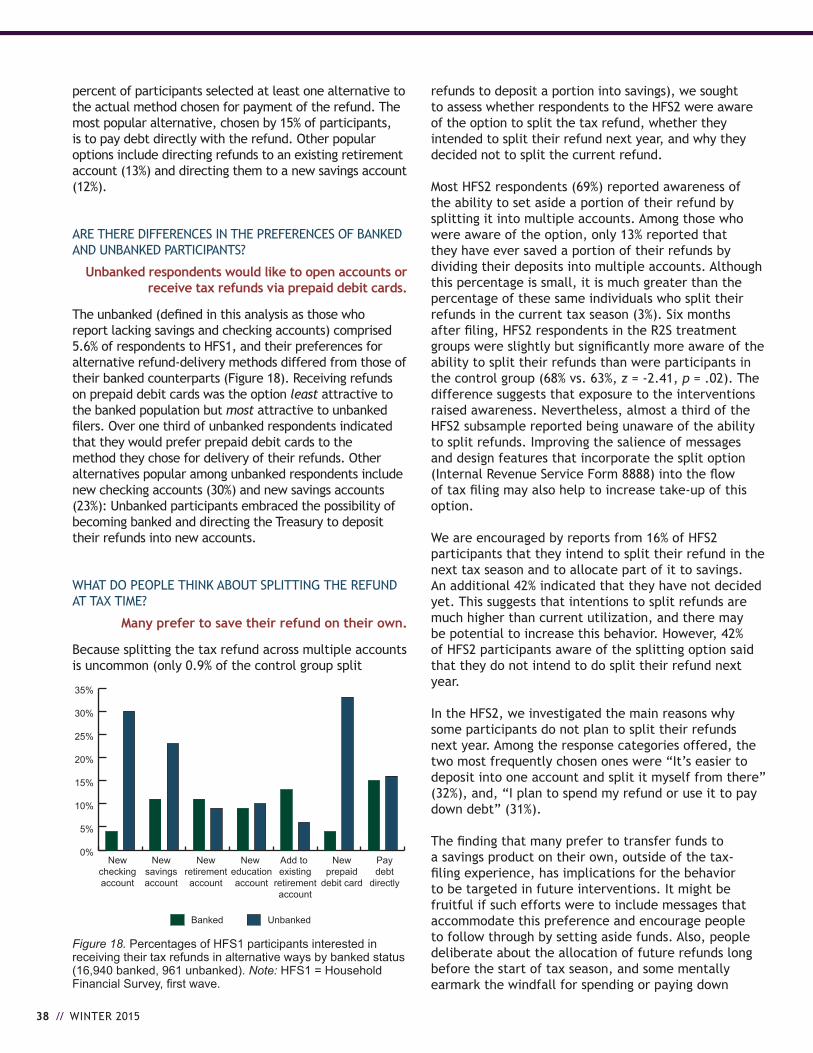
38 // WINTER 2015

percent of participants selected at least one alternative to the actual method chosen for payment of the refund. The most popular alternative, chosen by 15% of participants, is to pay debt directly with the refund. Other popular options include directing refunds to an existing retirement account (13%) and directing them to a new savings account (12%).

ARE THERE DIFFERENCES IN THE PREFERENCES OF BANKED AND UNBANKED PARTICIPANTS?

Unbanked respondents would like to open accounts or receive tax refunds via prepaid debit cards.

The unbanked (defined in this analysis as those who report lacking savings and checking accounts) comprised 5.6% of respondents to HFS1, and their preferences for alternative refund-delivery methods differed from those of their banked counterparts (Figure 18). Receiving refunds on prepaid debit cards was the option least attractive to the banked population but most attractive to unbanked filers. Over one third of unbanked respondents indicated that they would prefer prepaid debit cards to the method they chose for delivery of their refunds. Other alternatives popular among unbanked respondents include new checking accounts (30%) and new savings accounts (23%): Unbanked participants embraced the possibility of becoming banked and directing the Treasury to deposit their refunds into new accounts.

WHAT DO PEOPLE THINK ABOUT SPLITTINg THE REFUND AT TAX TIME?

Many prefer to save their refund on their own.

Because splitting the tax refund across multiple accounts is uncommon (only 0.9% of the control group split

refunds to deposit a portion into savings), we sought to assess whether respondents to the HFS2 were aware of the option to split the tax refund, whether they intended to split their refund next year, and why they decided not to split the current refund.

Most HFS2 respondents (69%) reported awareness of the ability to set aside a portion of their refund by splitting it into multiple accounts. Among those who were aware of the option, only 13% reported that they have ever saved a portion of their refunds by dividing their deposits into multiple accounts. Although this percentage is small, it is much greater than the percentage of these same individuals who split their refunds in the current tax season (3%). Six months after filing, HFS2 respondents in the R2S treatment groups were slightly but significantly more aware of the ability to split their refunds than were participants in the control group (68% vs. 63%, z = -2.41, p = .02). The difference suggests that exposure to the interventions raised awareness. Nevertheless, almost a third of the HFS2 subsample reported being unaware of the ability to split refunds. Improving the salience of messages and design features that incorporate the split option (Internal Revenue Service Form 8888) into the flow of tax filing may also help to increase take-up of this option.

We are encouraged by reports from 16% of HFS2 participants that they intend to split their refund in the next tax season and to allocate part of it to savings. An additional 42% indicated that they have not decided yet. This suggests that intentions to split refunds are much higher than current utilization, and there may be potential to increase this behavior. However, 42% of HFS2 participants aware of the splitting option said that they do not intend to do split their refund next year.

In the HFS2, we investigated the main reasons why some participants do not plan to split their refunds next year. Among the response categories offered, the two most frequently chosen ones were “It’s easier to deposit into one account and split it myself from there” (32%), and, “I plan to spend my refund or use it to pay down debt” (31%).

The finding that many prefer to transfer funds to a savings product on their own, outside of the tax-filing experience, has implications for the behavior to be targeted in future interventions. It might be fruitful if such efforts were to include messages that accommodate this preference and encourage people to follow through by setting aside funds. Also, people deliberate about the allocation of future refunds long before the start of tax season, and some mentally earmark the windfall for spending or paying down

0%

5%

10%

15%

20%

25%

30%

35%

UnbankedBanked

Paydebt

directly

Newprepaid

debit card

Add to existing

retirementaccount

New educationaccount

Newretirementaccount

Newsavingsaccount

Newcheckingaccount

Figure 18. Percentages of HFS1 participants interested in receiving their tax refunds in alternative ways by banked status (16,940 banked, 961 unbanked). Note: HFS1 = Household Financial Survey, first wave.

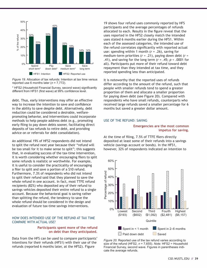
CSD.WUSTL.EDU // 39

debt. Thus, early interventions may offer an effective way to increase the intention to save and confidence in the ability to save despite debt. Alternatively, debt reduction could be considered a desirable, welfare-promoting behavior, and interventions could incorporate methods to help people address debt (e.g., promoting early filing to pay down debts sooner, facilitating direct deposits of tax refunds to retire debt, and providing advice on or referrals for debt consolidation).

An additional 19% of HFS2 respondents did not intend to split the refund next year because their “refund will be too small for it to make sense to split”; this suggests that, in evaluating success of the tax-time intervention, it is worth considering whether encouraging filers to split some refunds is realistic or worthwhile. For example, it is useful to consider the practicality of encouraging a filer to split and save a portion of a $10 refund. Furthermore, 7.3% of respondents who did not intend to split their refund said that they planned to save the whole refund in one account. In fact, most TTFE refund recipients (82%) who deposited any of their refund to savings vehicles deposited their entire refund to a single account. Because the behavioral goal is saving rather than splitting the refund, the tendency to save the whole refund should be considered in the design and evaluation of future tax-time savings interventions.

HOW DOES INTENDED USE OF THE REFUND AT TAX TIME COMPARE WITH ACTUAL USE?

Participants spent more of the refund on debt than they anticipated.

Data from the HFS can be used to compare participants’ intentions for their refunds (HFS1) with their use of the refunds (reported 6 months later, at the HFS2). Figure

19 shows four refund uses commonly reported by HFS participants and the average percentages of refunds allocated to each. Results in the figure reveal that the uses reported in the HFS2 closely match the intended uses stated 6 months earlier during the HFS1. Within each of the assessed categories, the intended use of the refund correlates significantly with reported actual use: spending within 1 month (r = .26), saving for medium-term priorities (r = .21), paying down debt (r = .41), and saving for the long term (r = .45; p < .0001 for all). Participants put more of their refund toward debt repayment than they intended at tax time, and they reported spending less than anticipated.

It is noteworthy that the reported uses of refunds differ according to the amount of the refund, such that people with smaller refunds tend to spend a greater proportion of them and allocate a smaller proportion for paying down debt (see Figure 20). Compared with respondents who have small refunds, counterparts who received large refunds saved a smaller percentage for 6 months but saved a greater dollar amount.

USE OF THE REFUND: SAVINg

Emergencies are the most common impetus for saving.

At the time of filing, 7.5% of TTFE filers directly deposited at least some of their refunds into a savings vehicle (savings account or bonds). In the HFS1, however, 32% of respondents indicated an intention to

0%

10%

20%

30%

40%

50%

HFS2: Reported useHFS1: Intention

Savelong term

Savemedium term*

Paydown debt*

Spendshort term*

% o

f the

refu

nd 32%

23%

33%

43%

22%19%

14% 14%

Figure 19. Allocation of tax refunds: Intention at tax time versus reported use 6 months later (n = 7,772). * HFS2 (Household Financial Survey, second wave) significantly different from HFS1 (first wave) at 99% confidence level.

0%

10%

20%

30%

40%

50%

60%

SavedPaid down debt

Spent in 2–6 monthsSpent in < 1 month

Highest ($6,157)

Fourth($2,481)

Third$1,092)

Second($602)

Lowest($193)

Quintile

Per

cent

age

of re

fund

(

Figure 20. Reported use of the tax refund varies according to size of the refund (HFS2, n = 7,655). Note: HFS2 = Household Financial Survey, second wave. Figures in parentheses indi-cate the average refunds.

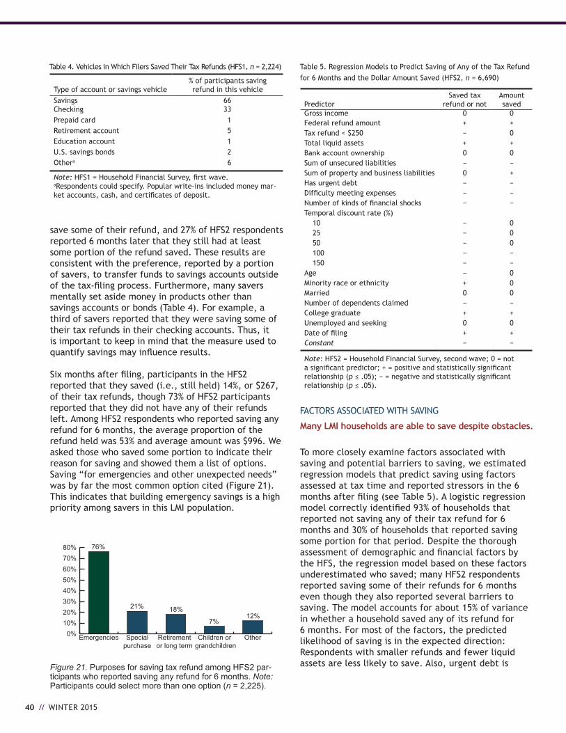
40 // WINTER 2015

save some of their refund, and 27% of HFS2 respondents reported 6 months later that they still had at least some portion of the refund saved. These results are consistent with the preference, reported by a portion of savers, to transfer funds to savings accounts outside of the tax-filing process. Furthermore, many savers mentally set aside money in products other than savings accounts or bonds (Table 4). For example, a third of savers reported that they were saving some of their tax refunds in their checking accounts. Thus, it is important to keep in mind that the measure used to quantify savings may influence results.

Six months after filing, participants in the HFS2 reported that they saved (i.e., still held) 14%, or $267, of their tax refunds, though 73% of HFS2 participants reported that they did not have any of their refunds left. Among HFS2 respondents who reported saving any refund for 6 months, the average proportion of the refund held was 53% and average amount was $996. We asked those who saved some portion to indicate their reason for saving and showed them a list of options. Saving “for emergencies and other unexpected needs” was by far the most common option cited (Figure 21). This indicates that building emergency savings is a high priority among savers in this LMI population.

0%10%20%30%40%50%60%70%80%

OtherChildren or grandchildren

Retirementor long term

Specialpurchase

Emergencies

76%

21% 18%

7%12%

Figure 21. Purposes for saving tax refund among HFS2 par-ticipants who reported saving any refund for 6 months. Note: Participants could select more than one option (n = 2,225).

Type of account or savings vehicle% of participants saving refund in this vehicle

Savings 66Checking 33Prepaid card 1Retirement account 5Education account 1U.S. savings bonds 2Othera 6

Note: HFS1 = Household Financial Survey, first wave.aRespondents could specify. Popular write-ins included money mar-ket accounts, cash, and certificates of deposit.

Table 4. Vehicles in Which Filers Saved Their Tax Refunds (HFS1, n = 2,224)

PredictorSaved tax

refund or notAmount saved

gross income 0 0Federal refund amount + +Tax refund < $250 − 0Total liquid assets + +Bank account ownership 0 0Sum of unsecured liabilities − −Sum of property and business liabilities 0 +Has urgent debt − −Difficulty meeting expenses − −Number of kinds of financial shocks − −Temporal discount rate (%)

10 − 025 − 050 − 0100 − −150 − −

Age − 0Minority race or ethnicity + 0Married 0 0Number of dependents claimed − −College graduate + +Unemployed and seeking 0 0Date of filing + +Constant − −

Note: HFS2 = Household Financial Survey, second wave; 0 = not a significant predictor; + = positive and statistically significant relationship (p ≤ .05); − = negative and statistically significant relationship (p ≤ .05).

Table 5. Regression Models to Predict Saving of Any of the Tax Refund for 6 Months and the Dollar Amount Saved (HFS2, n = 6,690)

FACTORS ASSOCIATED WITH SAVINg

Many LMI households are able to save despite obstacles.

To more closely examine factors associated with saving and potential barriers to saving, we estimated regression models that predict saving using factors assessed at tax time and reported stressors in the 6 months after filing (see Table 5). A logistic regression model correctly identified 93% of households that reported not saving any of their tax refund for 6 months and 30% of households that reported saving some portion for that period. Despite the thorough assessment of demographic and financial factors by the HFS, the regression model based on these factors underestimated who saved; many HFS2 respondents reported saving some of their refunds for 6 months even though they also reported several barriers to saving. The model accounts for about 15% of variance in whether a household saved any of its refund for 6 months. For most of the factors, the predicted likelihood of saving is in the expected direction: Respondents with smaller refunds and fewer liquid assets are less likely to save. Also, urgent debt is

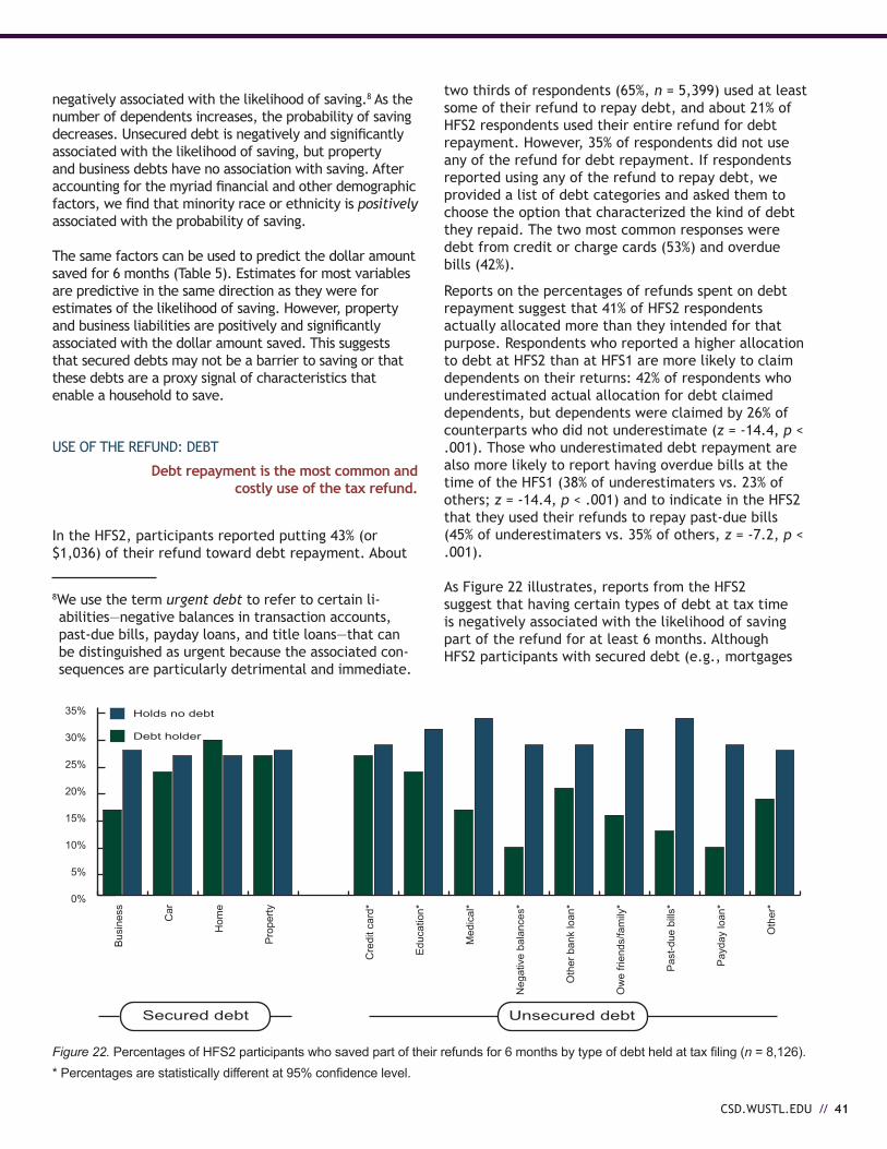
CSD.WUSTL.EDU // 41

two thirds of respondents (65%, n = 5,399) used at least some of their refund to repay debt, and about 21% of HFS2 respondents used their entire refund for debt repayment. However, 35% of respondents did not use any of the refund for debt repayment. If respondents reported using any of the refund to repay debt, we provided a list of debt categories and asked them to choose the option that characterized the kind of debt they repaid. The two most common responses were debt from credit or charge cards (53%) and overdue bills (42%).

Reports on the percentages of refunds spent on debt repayment suggest that 41% of HFS2 respondents actually allocated more than they intended for that purpose. Respondents who reported a higher allocation to debt at HFS2 than at HFS1 are more likely to claim dependents on their returns: 42% of respondents who underestimated actual allocation for debt claimed dependents, but dependents were claimed by 26% of counterparts who did not underestimate (z = -14.4, p < .001). Those who underestimated debt repayment are also more likely to report having overdue bills at the time of the HFS1 (38% of underestimaters vs. 23% of others; z = -14.4, p < .001) and to indicate in the HFS2 that they used their refunds to repay past-due bills (45% of underestimaters vs. 35% of others, z = -7.2, p < .001).

As Figure 22 illustrates, reports from the HFS2 suggest that having certain types of debt at tax time is negatively associated with the likelihood of saving part of the refund for at least 6 months. Although HFS2 participants with secured debt (e.g., mortgages

negatively associated with the likelihood of saving.8 As the number of dependents increases, the probability of saving decreases. Unsecured debt is negatively and significantly associated with the likelihood of saving, but property and business debts have no association with saving. After accounting for the myriad financial and other demographic factors, we find that minority race or ethnicity is positively associated with the probability of saving.

The same factors can be used to predict the dollar amount saved for 6 months (Table 5). Estimates for most variables are predictive in the same direction as they were for estimates of the likelihood of saving. However, property and business liabilities are positively and significantly associated with the dollar amount saved. This suggests that secured debts may not be a barrier to saving or that these debts are a proxy signal of characteristics that enable a household to save.

USE OF THE REFUND: DEBT

Debt repayment is the most common and costly use of the tax refund.

In the HFS2, participants reported putting 43% (or $1,036) of their refund toward debt repayment. About

8 We use the term urgent debt to refer to certain li-abilities—negative balances in transaction accounts, past-due bills, payday loans, and title loans—that can be distinguished as urgent because the associated con-sequences are particularly detrimental and immediate.

Figure 22. Percentages of HFS2 participants who saved part of their refunds for 6 months by type of debt held at tax filing (n = 8,126). * Percentages are statistically different at 95% confidence level.

0%

5%

10%

15%

20%

25%

30%

35% Holds no debt

Debt holder

Oth

er*

Pay

day

loan

*

Pas

t-due

bill

s*

Ow

e fri

ends

/fam

ily*

Oth

er b

ank

loan

*

Neg

ativ

e ba

lanc

es*

Med

ical

*

Edu

catio

n*

Cre

dit c

ard*

Pro

perty

Hom

e

Car

Bus

ines

s

Secured debt Unsecured debt

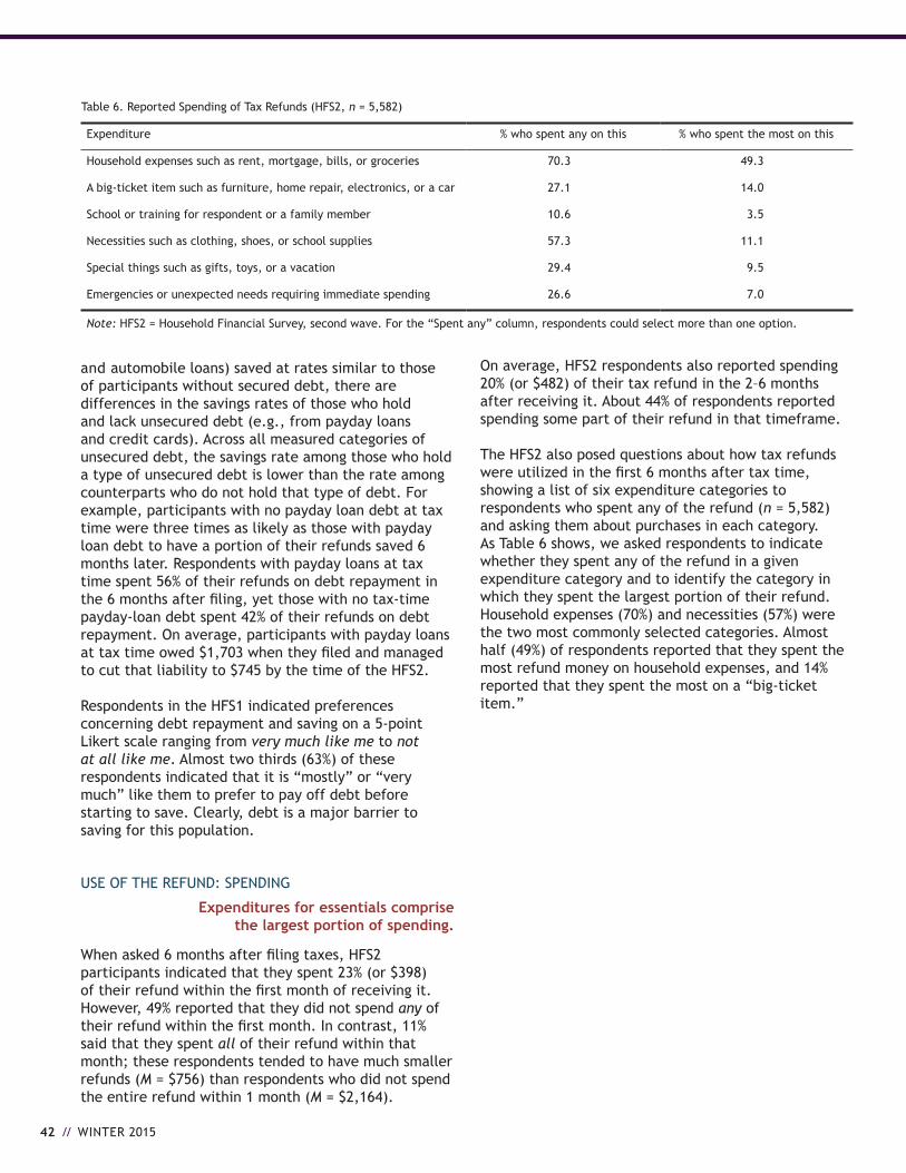
42 // WINTER 2015

and automobile loans) saved at rates similar to those of participants without secured debt, there are differences in the savings rates of those who hold and lack unsecured debt (e.g., from payday loans and credit cards). Across all measured categories of unsecured debt, the savings rate among those who hold a type of unsecured debt is lower than the rate among counterparts who do not hold that type of debt. For example, participants with no payday loan debt at tax time were three times as likely as those with payday loan debt to have a portion of their refunds saved 6 months later. Respondents with payday loans at tax time spent 56% of their refunds on debt repayment in the 6 months after filing, yet those with no tax-time payday-loan debt spent 42% of their refunds on debt repayment. On average, participants with payday loans at tax time owed $1,703 when they filed and managed to cut that liability to $745 by the time of the HFS2.

Respondents in the HFS1 indicated preferences concerning debt repayment and saving on a 5-point Likert scale ranging from very much like me to not at all like me. Almost two thirds (63%) of these respondents indicated that it is “mostly” or “very much” like them to prefer to pay off debt before starting to save. Clearly, debt is a major barrier to saving for this population.

USE OF THE REFUND: SPENDINg

Expenditures for essentials comprise the largest portion of spending.

When asked 6 months after filing taxes, HFS2 participants indicated that they spent 23% (or $398) of their refund within the first month of receiving it. However, 49% reported that they did not spend any of their refund within the first month. In contrast, 11% said that they spent all of their refund within that month; these respondents tended to have much smaller refunds (M = $756) than respondents who did not spend the entire refund within 1 month (M = $2,164).

On average, HFS2 respondents also reported spending 20% (or $482) of their tax refund in the 2–6 months after receiving it. About 44% of respondents reported spending some part of their refund in that timeframe.

The HFS2 also posed questions about how tax refunds were utilized in the first 6 months after tax time, showing a list of six expenditure categories to respondents who spent any of the refund (n = 5,582) and asking them about purchases in each category. As Table 6 shows, we asked respondents to indicate whether they spent any of the refund in a given expenditure category and to identify the category in which they spent the largest portion of their refund. Household expenses (70%) and necessities (57%) were the two most commonly selected categories. Almost half (49%) of respondents reported that they spent the most refund money on household expenses, and 14% reported that they spent the most on a “big-ticket item.”

Expenditure % who spent any on this % who spent the most on this

Household expenses such as rent, mortgage, bills, or groceries 70.3 49.3

A big-ticket item such as furniture, home repair, electronics, or a car 27.1 14.0

School or training for respondent or a family member 10.6 3.5

Necessities such as clothing, shoes, or school supplies 57.3 11.1

Special things such as gifts, toys, or a vacation 29.4 9.5

Emergencies or unexpected needs requiring immediate spending 26.6 7.0

Note: HFS2 = Household Financial Survey, second wave. For the “Spent any” column, respondents could select more than one option.

Table 6. Reported Spending of Tax Refunds (HFS2, n = 5,582)

CSD.WUSTL.EDU // 43

VIII. ThE FINANCIAl lIVES OF lmI hOUSEhOlDS

The HFS included a thorough ascertainment of household assets and liabilities. The details of these data offer an in-depth understanding of the challenging context that awaits policies to benefit the financial well-being of LMI households.

THE BALANCE SHEET

More than one in 10 HFS1 respondents reported having no liquid assets (i.e., money in checking or savings accounts, or cash saved at home), and the median value of liquid assets reported by HFS1 respondents was only $550. In this context, it is not surprising that 61% of the HFS1 subsample indicated being “certainly” or “probably” unable to come up with $2,000 in an emergency. It is notable that HFS1 respondents reported average regular monthly expenses of $1,725 (the median was $1,500). The R2S team also asked respondents what the minimum monthly household expense would be “if you were to tighten your belt as much as possible.” The average minimum reported by HFS1 participants was $1,431 (the median was $1,250). The relatively minor difference between the reported typical and minimum expenses suggests that many households have already minimized expenditures. About three quarters (77%) of HFS1

respondents indicated that they found it “somewhat” or “very” difficult to cover expenses and pay all of their bills in a typical month.

ASSETS

More than a quarter of HFS1 respondents lack a savings account.

In the HFS1 subsample, the sum value of all nonproperty and nonbusiness assets was modest. The median value was $1,300. Table 7 shows a summary of assets reportedly held at the time of the HFS1. Most respondents had holdings in checking and savings accounts; however, 29% had no savings account and 5.6% were unbanked. Being unbanked poses a technical barrier at the time of tax filing, making it difficult for filers to use direct deposit or to split part of a refund directly into savings.

Relatively few HFS1 respondents held any assets in investments such as stocks, mutual funds, money market accounts, brokerage accounts, or annuities. The low rates of investment among HFS1 respondents closely resemble, but are lower than, national participation rates among low-income households: Stock ownership was reported by 10.6% of HFS1 respondents and by 15% of LMI households in the U.S. population (Tyson, 2013); 6.6% of respondents and 12% of LMI households in the United States reportedly own mutual funds (Burham, Bogdan, & Schrass, 2013).

Holdings % with this asset Mean value ($) Median value ($)

AssetsPhysical assetsHome 22.1 103,222 90,000Other property 4.5 152,503 75,000Car 85.2 9,089 5,500Business 2.8 96,280 10,000

Nonproperty assetsChecking 92.2 1,530 500Savings 70.9 2,754 300Unused balance on prepaid card 15.1 329 50Retirement account, IRA, or 401(k) 40.4 31,806 6,000Certificates of deposit 5.2 11,722 4,200Money market account 6.9 9,738 3,000Mutual fund or hedge fund 6.6 25,508 9,000Savings bond 11.3 1,314 400Other bond such as corporate or treasury 1.7 6,475 1,250Stocks 10.6 10,538 2,000Education account (e.g., 529 Coverdell) 2.5 9,634 3,800Cash saved at home 23.7 474 200Loans owed to participant by others 9.1 3,193 1,000Brokerage accounts 3.5 40,874 8,375Annuities 2.9 42,361 18,000Othera 1.8 30,276 8,000

Note: HFS1 = Household Financial Survey, first wave. Dollar amounts shown are among people with holdings in that asset. Outliers above 99th percentile for each category were omitted.

aRespondents could specify. The most common write-ins were tangible assets (e.g., art, jewelry, guns).

Table 7. Reported Holdings of HFS1 Participants at Tax Time

44 // WINTER 2015

yet, the value of holdings by the few HFS respondents with such assets tends to be in the thousands of dollars.

RETIREMENT SAVINgS

Even those approaching traditional retirement age are not financially prepared to retire.

About four in 10 respondents in the HFS1 reported having an IRA or other retirement account such as a 401(k); this is about the same as the rate for the general population in the United States but significantly higher than the rate (12%) among low-income U.S. households (Investment Company Institute, 2010). More than half (54%) of HFS1 respondents over age 50 (n = 4,610) have no retirement funds. In the TTFE data, 8.1% of tax filers claimed credits for retirement savings contributions and 8.9% reported income from retirement distributions. About half (48%) of those reporting retirement-distribution income were younger than age 60 at the time of the first survey, and this may suggest that many paid a penalty on the distribution. On average, the retirement accounts of HFS1 respondents held approximately $32,000, and the median was $6,000. The large difference between the mean and median may indicate that large outliers drove up the mean value. Low balances in the retirement savings of the HFS1 subsample seem to suggest the benefits of creating mechanisms to divert tax refunds directly to retirement accounts such as IRAs.

HOUSINg AND PROPERTy

Most households that own homes were unable to claim mortgage-interest deductions.

Just 22% of HFS1 respondents were homeowners (n = 4,552), and the median estimated home value was $90,000 (results not shown). Two thirds of homeowners

in the HFS1 (66%) reported holding a home mortgage, and the median amount owed was $70,000. The median amount of home equity among these homeowners was $18,000. About one in seven HFS1 homeowners (15%) was “under water”—that is, they owed more on the mortgage than the estimated value of the home. Because they did not itemize their tax returns, 79% of respondents repaying mortgages were unable to take mortgage-interest deductions. Our analysis suggests that these respondents had no tax liability or that the standard deduction was larger than an itemized deduction. This finding is consistent with reports by others that mortgage-interest deduction policy disproportionately benefits high-earning households (Toder, Turner, Lim, & Getsinger, 2010). About 6.3% of HFS1 respondents reported living in situations that do not require them to make monthly payments for rent or a mortgage. Among those who did make housing payments, the average monthly payment was $790 (median $700). A quarter of the HFS1 subsample (25%) reported being unable to make the full payment for rent or mortgage at some point in the last year.

Most HFS1 respondents reported owning a car (85%), and 38% of those were making monthly car payments at the time of the survey. Less than 3% of this subsample reported business-related assets or liabilities. Only 4.5% reported owning property other than their primary residences.

LIABILITIES

The debts of most HFS1 respondents exceed their assets.

The HFS assessment of liabilities suggests that many LMI households have been coping with heavy burdens (see Table 8). Their survey responses depict an environment in which the ability to save and the perceived ability to

Type of debt % with this debt Mean value ($) Median value ($)

SecuredHome 14.5 78,932 70,000Other property 1.3 97,039 70,000Car 32.6 10,172 8,200Business 0.3 47,944 12,500UnsecuredCredit or charge card 63.3 4,513 2,000Education or school loan 51.0 31,173 20,000Personal loan from family or friend 24.6 3,419 1,500Personal loan from bank or credit union 15.3 7,726 3,500Payday or title loan 8.0 1,227 650Unpaid medical bill 42.2 5,054 1,500Past-due regular bill or rent 33.4 1,067 500Negative balance in checking or savings 8.5 355 200

Note: HFS1 = Household Financial Survey, first wave. Dollar amounts shown are among those who had that kind of debt. Outliers above 99th percentile for each category were omitted.

Table 8. Reported Debts and Liabilities of HFS1 Respondents at Tax Time (HFS1)

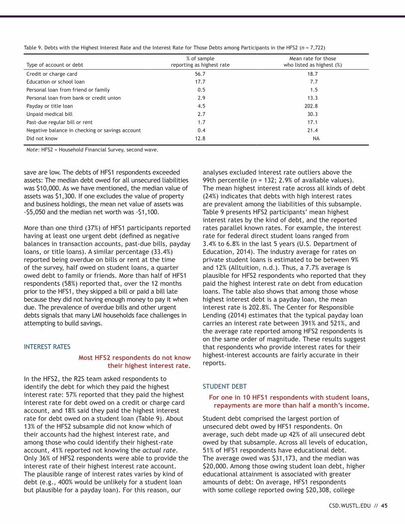
CSD.WUSTL.EDU // 45

save are low. The debts of HFS1 respondents exceeded assets: The median debt owed for all unsecured liabilities was $10,000. As we have mentioned, the median value of assets was $1,300. If one excludes the value of property and business holdings, the mean net value of assets was -$5,050 and the median net worth was -$1,100.

More than one third (37%) of HFS1 participants reported having at least one urgent debt (defined as negative balances in transaction accounts, past-due bills, payday loans, or title loans). A similar percentage (33.4%) reported being overdue on bills or rent at the time of the survey, half owed on student loans, a quarter owed debt to family or friends. More than half of HFS1 respondents (58%) reported that, over the 12 months prior to the HFS1, they skipped a bill or paid a bill late because they did not having enough money to pay it when due. The prevalence of overdue bills and other urgent debts signals that many LMI households face challenges in attempting to build savings.

INTEREST RATES

Most HFS2 respondents do not know their highest interest rate.

In the HFS2, the R2S team asked respondents to identify the debt for which they paid the highest interest rate: 57% reported that they paid the highest interest rate for debt owed on a credit or charge card account, and 18% said they paid the highest interest rate for debt owed on a student loan (Table 9). About 13% of the HFS2 subsample did not know which of their accounts had the highest interest rate, and among those who could identify their highest-rate account, 41% reported not knowing the actual rate. Only 36% of HFS2 respondents were able to provide the interest rate of their highest interest rate account. The plausible range of interest rates varies by kind of debt (e.g., 400% would be unlikely for a student loan but plausible for a payday loan). For this reason, our

analyses excluded interest rate outliers above the 99th percentile (n = 132; 2.9% of available values). The mean highest interest rate across all kinds of debt (24%) indicates that debts with high interest rates are prevalent among the liabilities of this subsample. Table 9 presents HFS2 participants’ mean highest interest rates by the kind of debt, and the reported rates parallel known rates. For example, the interest rate for federal direct student loans ranged from 3.4% to 6.8% in the last 5 years (U.S. Department of Education, 2014). The industry average for rates on private student loans is estimated to be between 9% and 12% (Alltuition, n.d.). Thus, a 7.7% average is plausible for HFS2 respondents who reported that they paid the highest interest rate on debt from education loans. The table also shows that among those whose highest interest debt is a payday loan, the mean interest rate is 202.8%. The Center for Responsible Lending (2014) estimates that the typical payday loan carries an interest rate between 391% and 521%, and the average rate reported among HFS2 respondents is on the same order of magnitude. These results suggest that respondents who provide interest rates for their highest-interest accounts are fairly accurate in their reports.

STUDENT DEBT

For one in 10 HFS1 respondents with student loans, repayments are more than half a month’s income.

Student debt comprised the largest portion of unsecured debt owed by HFS1 respondents. On average, such debt made up 42% of all unsecured debt owed by that subsample. Across all levels of education, 51% of HFS1 respondents have educational debt. The average owed was $31,173, and the median was $20,000. Among those owing student loan debt, higher educational attainment is associated with greater amounts of debt: On average, HFS1 respondents with some college reported owing $20,308, college

Type of account or debt% of sample

reporting as highest rateMean rate for those

who listed as highest (%)

Credit or charge card 56.7 18.7Education or school loan 17.7 7.7

Personal loan from friend or family 0.5 1.5

Personal loan from bank or credit union 2.9 13.3

Payday or title loan 4.5 202.8

Unpaid medical bill 2.7 30.3

Past-due regular bill or rent 1.7 17.1

Negative balance in checking or savings account 0.4 21.4

Did not know 12.8 NA

Note: HFS2 = Household Financial Survey, second wave.

Table 9. Debts with the Highest Interest Rate and the Interest Rate for Those Debts among Participants in the HFS2 (n = 7,722)

46 // WINTER 2015

graduates reported owing $31,483, and respondents with a graduate degree or professional education reported owing $60,036.

Among HSF1 respondents who were repaying student loans and were no longer students at the time of that survey, 35% indicated that they were not college graduates. Lacking the benefits of a degree, those who did not graduate may have a hard time repaying student loans. Furthermore, other research shows that debt itself can play a part in the decision not to complete college (Dwyer, McCloud, & Hodson, 2012).

The burden from student debt varies significantly by race. To investigate this variation, we estimated a regression using HFS1 data. The results suggest that the average student-debt burden of an African American graduating from college at age 22 would be $31,498—over $7,800 more than that of a White college graduate of the same age and $11,000 more than that of an Asian counterpart. These racial disparities in debt from postsecondary education resemble outcomes found elsewhere (Jackson & Reynolds, 2013; Price, 2004; Zeiser, Kirshstein, & Tanenbaum, 2013).

Monthly payments toward educational debt also tend to be high in relation to income for this sample of LMI households. Among HFS1 participants reporting educational debt, the average monthly student loan payment was just over $220 and the median was $150. These households reported allocating a median of 11% of monthly income (and a mean of 26%) for repayment of educational debt. For 10% of student loan holders in the HFS1, the reported debt repayment exceeds 50% of monthly household income. Such repayments far exceed the 8% industry standard often used as a threshold to determine monthly repayment structures (Baum & Schwartz, 2006) and the 10% level used in income-based repayment plans for federal student loans (Federal Student Aid, 2014). Likewise, TTFE data suggest that annual education expenses are high, yet it is encouraging that about seven in 10 enrolled students

took advantage of tax deductions for educational expenses. On average, HFS1 respondents claimed deductions for $10,230 in expenditures on items like books, fees, and tuition (median = $5,967).

HEALTH CARE

Monetary constraints prevent many people from receiving necessary medical care.

Financial hardships significantly affect the ability of HFS1 respondents to receive proper medical care. Forty-five percent of HFS1 respondents reported that, in the year prior to the survey, financial reasons prompted them to forgo a visit to a doctor or hospital when they needed such a visit. One third (33%) reported skipping or postponing necessary prescription medications, and 52% reported that they were unable to afford a needed visit to a dentist. Participants estimated that their mean out-of-pocket medical costs in the previous year were $1,455 and the median was $500. About 42% of HFS1 participants reported medical debt. The average amount of such debt was more than $5,000, and the median was $1,500. More than a quarter of HFS2 respondents (27%) indicated that they had no health insurance. In the HFS2 subsample, the most commonly reported health insurance coverage was provided by an employer (42%), 8.4% of the subsample was covered by Medicaid, and 5.0% was covered through Medicare (see Table 10).

Insurance type% of

sampleUninsured 26.7Through employer 42.1Medicaid 8.4Medicare 5.0Private or direct 4.9Student or school plan 4.3Other (specified)On parent or family plan 5.4Military-related (e.g., Veterans Administration, Tricare) 1.3State, county, tribal, or other government 1.2Other 0.6

Note: HFS2 = Household Financial Survey, second wave.

Table 10. Types of Health Insurance Coverage Reported in the HFS2 (n = 8,189)

CSD.WUSTL.EDU // 47

Ix. COpING wITh lACk OF SAVINGSOur data show that LMI households frequently experience unexpected financial emergencies. In the absence of sufficient contingency savings to contend with such events, households must cope by coming up with funds (often from financially penalizing alternative sources), falling behind on bills, or cutting back on material necessities. In this way, as detailed below, the lack of savings may compound and prolong the financial and personal hardships faced by LMI households.

VOLATILITy

Two thirds of respondents experienced a financial shock in the 6 months after filing taxes.

At the time of tax filing, 11% of HFS1 respondents were unemployed and looking for work; this compares with a nationwide unemployment rate of about 7.6% over the same period (February–April 2013; Bureau of Labor Statistics 2014a). Six months later, 34% of HFS2 participants who previously reported that they were unemployed indicated that they were working full time. An additional 20% reported working part time, 31% said that they were still unemployed and looking; and 6.7% told us that they were unemployed but no longer looking for a job. About one third of HFS2 respondents (33%) indicated that someone in their household experienced a period of unemployment between the first and second waves of the survey, and 36% reported that a household member started a new job or changed jobs within the last 6 months. In the same 6-month period, 22% of respondents changed residences, and 47% of these respondents moved away from the city or town in which they were living when they filed taxes.

Approximately two thirds of HFS2 households reported that they experienced a financial emergency, such as a trip to the hospital, major vehicle repair, period of unemployment, or legal expense, in the 6 months since filing their tax returns (see Figure 23). The high prevalence of these emergencies in the 6 months following tax filing is important because almost 60% of the 20,000 tax filers who completed the HFS1 survey at tax time said that they could not come up with $2,000 within 30 days if they needed to cover a financial emergency.

ALTERNATIVE FINANCIAL SERVICES

Use of alternative financial services is lower among respondents who have credit cards

than among those who lack them.

In order to cope with the emergencies that arose, many of these LMI taxpayers used high-risk, high-cost options—choices with the potential to negatively affect financial strength and household well-being in both the short term and the long run. Alternative financial services are an array of controversial services provided by nonbank financial institutions. In assessing the use of such services, the HFS distinguishes alternative financial transaction services—check cashing, money orders, payroll cards (payment for wages on debit cards), and remittance (out of country wire transfers via nonbank institutions)—from alternative financial credit services: payday loans, auto title loans, refund-anticipation loans, pawning, and rent-to-own arrangements. In general, alternative financial transaction services provide banking services via nontraditional institutions, whereas alternative financial credit services provide immediate access to liquid funds. All of these services, especially the credit services, are usually associated with high fees or high interest rates (Fellowes & Mabanta, 2008; Temkin & Sawyer, 2004).

Similar to previous research in this area (see, e.g., Federal Deposit Insurance Corporation, 2013a), results from the HFS1 show that a large proportion of respondent households use alternative financial services (Figure 24). About 41% of HFS1 respondents reported using such a service in the 12 months prior to the survey. The rate for the use of alternative transaction services is comparable with that for the use of alternative credit services: 30% of HFS1 respondents reported using an alternative transaction service in the year prior to the survey, and 28% reported using an alternative credit service over that period.

Certain factors assessed by the HFS1 are associated with the reported use of alternative financial services in the 6 months after filing taxes (assessed by HFS2):

0

10%

20%

30%

40%

50%

60%

70%

80%

Any

fina

ncia

lsh

ock

Lega

l fee

s o

r exp

ense

s

Per

iod

ofun

empl

oym

ent

Maj

or v

ehic

lere

pair

Trip

toho

spita

l

27%

36% 33%

9%

66%

Figure 23. Percentage of households experiencing financial shocks in the 6 months after filing taxes (n = 8,253).

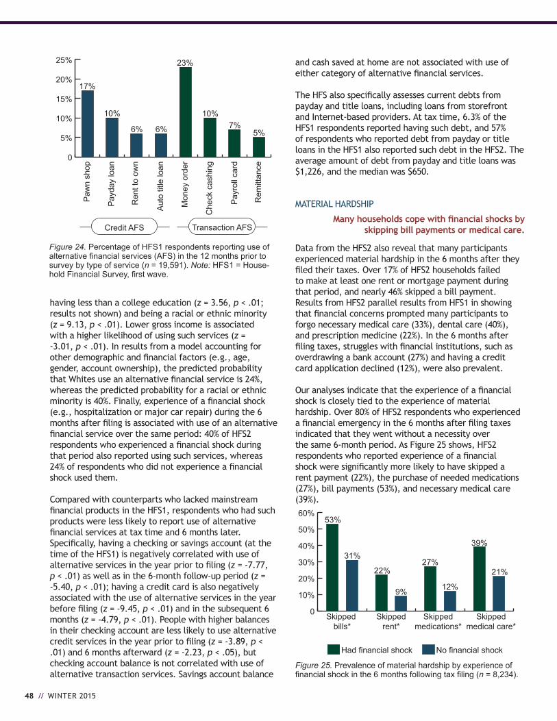
48 // WINTER 2015

having less than a college education (z = 3.56, p < .01; results not shown) and being a racial or ethnic minority (z = 9.13, p < .01). Lower gross income is associated with a higher likelihood of using such services (z = -3.01, p < .01). In results from a model accounting for other demographic and financial factors (e.g., age, gender, account ownership), the predicted probability that Whites use an alternative financial service is 24%, whereas the predicted probability for a racial or ethnic minority is 40%. Finally, experience of a financial shock (e.g., hospitalization or major car repair) during the 6 months after filing is associated with use of an alternative financial service over the same period: 40% of HFS2 respondents who experienced a financial shock during that period also reported using such services, whereas 24% of respondents who did not experience a financial shock used them.

Compared with counterparts who lacked mainstream financial products in the HFS1, respondents who had such products were less likely to report use of alternative financial services at tax time and 6 months later. Specifically, having a checking or savings account (at the time of the HFS1) is negatively correlated with use of alternative services in the year prior to filing (z = -7.77, p < .01) as well as in the 6-month follow-up period (z = -5.40, p < .01); having a credit card is also negatively associated with the use of alternative services in the year before filing (z = -9.45, p < .01) and in the subsequent 6 months (z = -4.79, p < .01). People with higher balances in their checking account are less likely to use alternative credit services in the year prior to filing (z = -3.89, p < .01) and 6 months afterward (z = -2.23, p < .05), but checking account balance is not correlated with use of alternative transaction services. Savings account balance

and cash saved at home are not associated with use of either category of alternative financial services.

The HFS also specifically assesses current debts from payday and title loans, including loans from storefront and Internet-based providers. At tax time, 6.3% of the HFS1 respondents reported having such debt, and 57% of respondents who reported debt from payday or title loans in the HFS1 also reported such debt in the HFS2. The average amount of debt from payday and title loans was $1,226, and the median was $650.

MATERIAL HARDSHIP

Many households cope with financial shocks by skipping bill payments or medical care.

Data from the HFS2 also reveal that many participants experienced material hardship in the 6 months after they filed their taxes. Over 17% of HFS2 households failed to make at least one rent or mortgage payment during that period, and nearly 46% skipped a bill payment. Results from HFS2 parallel results from HFS1 in showing that financial concerns prompted many participants to forgo necessary medical care (33%), dental care (40%), and prescription medicine (22%). In the 6 months after filing taxes, struggles with financial institutions, such as overdrawing a bank account (27%) and having a credit card application declined (12%), were also prevalent.

Our analyses indicate that the experience of a financial shock is closely tied to the experience of material hardship. Over 80% of HFS2 respondents who experienced a financial emergency in the 6 months after filing taxes indicated that they went without a necessity over the same 6-month period. As Figure 25 shows, HFS2 respondents who reported experience of a financial shock were significantly more likely to have skipped a rent payment (22%), the purchase of needed medications (27%), bill payments (53%), and necessary medical care (39%).

0

10%

20%

30%

40%

50%

60%

No financial shockHad financial shock

Skippedmedical care*

Skippedmedications*

Skippedrent*

Skipped bills*

53%

31%

22%

9%

27%

12%

21%

39%

Figure 25. Prevalence of material hardship by experience of financial shock in the 6 months following tax filing (n = 8,234).

0

5%

10%

15%

20%

25%

Rem

ittan

ce

Pay

roll

card

Che

ck c

ashi

ng

Mon

ey o

rder

Aut

o tit

le lo

an

Ren

t to

own

Pay

day

loan

Paw

n sh

op

Credit AFS Transaction AFS

17%

10%

6% 6%

23%

10%7%

5%

Figure 24. Percentage of HFS1 respondents reporting use of alternative financial services (AFS) in the 12 months prior to survey by type of service (n = 19,591). Note: HFS1 = House-hold Financial Survey, first wave.

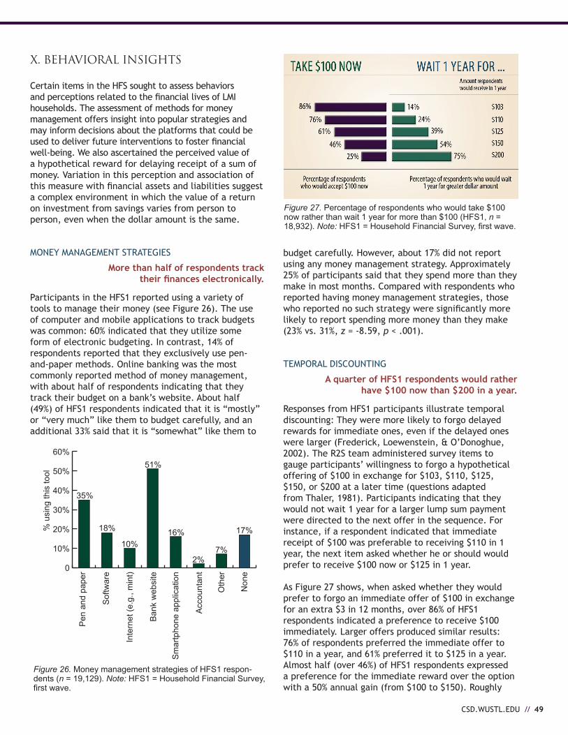
CSD.WUSTL.EDU // 49

x. BEhAVIORAl INSIGhTS

Certain items in the HFS sought to assess behaviors and perceptions related to the financial lives of LMI households. The assessment of methods for money management offers insight into popular strategies and may inform decisions about the platforms that could be used to deliver future interventions to foster financial well-being. We also ascertained the perceived value of a hypothetical reward for delaying receipt of a sum of money. Variation in this perception and association of this measure with financial assets and liabilities suggest a complex environment in which the value of a return on investment from savings varies from person to person, even when the dollar amount is the same.

MONEy MANAgEMENT STRATEgIES

More than half of respondents track their finances electronically.

Participants in the HFS1 reported using a variety of tools to manage their money (see Figure 26). The use of computer and mobile applications to track budgets was common: 60% indicated that they utilize some form of electronic budgeting. In contrast, 14% of respondents reported that they exclusively use pen-and-paper methods. Online banking was the most commonly reported method of money management, with about half of respondents indicating that they track their budget on a bank’s website. About half (49%) of HFS1 respondents indicated that it is “mostly” or “very much” like them to budget carefully, and an additional 33% said that it is “somewhat” like them to

budget carefully. However, about 17% did not report using any money management strategy. Approximately 25% of participants said that they spend more than they make in most months. Compared with respondents who reported having money management strategies, those who reported no such strategy were significantly more likely to report spending more money than they make (23% vs. 31%, z = -8.59, p < .001).

TEMPORAL DISCOUNTINg

A quarter of HFS1 respondents would rather have $100 now than $200 in a year.

Responses from HFS1 participants illustrate temporal discounting: They were more likely to forgo delayed rewards for immediate ones, even if the delayed ones were larger (Frederick, Loewenstein, & O’Donoghue, 2002). The R2S team administered survey items to gauge participants’ willingness to forgo a hypothetical offering of $100 in exchange for $103, $110, $125, $150, or $200 at a later time (questions adapted from Thaler, 1981). Participants indicating that they would not wait 1 year for a larger lump sum payment were directed to the next offer in the sequence. For instance, if a respondent indicated that immediate receipt of $100 was preferable to receiving $110 in 1 year, the next item asked whether he or should would prefer to receive $100 now or $125 in 1 year.

As Figure 27 shows, when asked whether they would prefer to forgo an immediate offer of $100 in exchange for an extra $3 in 12 months, over 86% of HFS1 respondents indicated a preference to receive $100 immediately. Larger offers produced similar results: 76% of respondents preferred the immediate offer to $110 in a year, and 61% preferred it to $125 in a year. Almost half (over 46%) of HFS1 respondents expressed a preference for the immediate reward over the option with a 50% annual gain (from $100 to $150). Roughly

0

10%

20%

30%

40%

50%

60%

Non

e

Oth

er

Acc

ount

ant

Sm

artp

hone

app

licat

ion

Ban

k w

ebsi

te

Inte

rnet

(e.g

., m

int)

Sof

twar

e

Pen

and

pap

er

35%

18%

10%

51%

16%

2%7%

17%% u

sing

this

tool

Figure 26. Money management strategies of HFS1 respon-dents (n = 19,129). Note: HFS1 = Household Financial Survey, first wave.

Figure 27. Percentage of respondents who would take $100 now rather than wait 1 year for more than $100 (HFS1, n = 18,932). Note: HFS1 = Household Financial Survey, first wave.

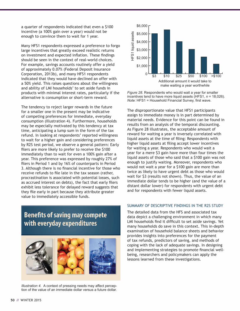
50 // WINTER 2015

a quarter of respondents indicated that even a $100 incentive (a 100% gain over a year) would not be enough to convince them to wait for 1 year.

Many HFS1 respondents expressed a preference to forgo large incentives that greatly exceed realistic returns on investment and expected inflation. These findings should be seen in the context of real-world choices. For example, savings accounts routinely offer a yield of approximately 0.07% (Federal Deposit Insurance Corporation, 2013b), and many HFS1 respondents indicated that they would have declined an offer with a 50% yield. This raises questions about the willingness and ability of LMI households’ to set aside funds in products with minimal interest rates, particularly if the alternative is consumption or short-term reward.

The tendency to reject larger rewards in the future for a smaller one in the present may be indicative of competing preferences for immediate, everyday consumption (Illustration 4). Furthermore, households may be especially motivated by this tendency at tax time, anticipating a lump sum in the form of the tax refund. In looking at respondents’ reported willingness to wait for a higher gain and considering preferences by R2S test period, we observe a general pattern: Early filers are more likely to prefer to receive the $100 immediately than to wait for even a 100% gain after a year. This preference was expressed by roughly 27% of filers in Period 1 and by 16% of counterparts in Period 3. Although there is no financial incentive for those who receive refunds to file late in the tax season (rather, procrastination is associated with potential losses, such as accrued interest on debts), the fact that early filers exhibit less tolerance for delayed reward suggests that they file early in part because they attribute greater value to immediately accessible funds.

The disproportionate value that HFS1 participants assign to immediate money is in part determined by material needs. Evidence for this point can be found in results from an analysis of the temporal discounting. As Figure 28 illustrates, the acceptable amount of reward for waiting a year is inversely correlated with liquid assets at the time of filing: Respondents with higher liquid assets at filing accept lower incentives for waiting a year. Respondents who would wait a year for a mere $3 gain have more than four times the liquid assets of those who said that a $100 gain was not enough to justify waiting. Moreover, respondents who would not wait a year for a $100 gain are more than twice as likely to have urgent debt as those who would wait for $3 (results not shown). Thus, the value of an immediate dollar tends to be higher (and the value of a distant dollar lower) for respondents with urgent debt and for respondents with fewer liquid assets.

SUMMARy OF DESCRIPTIVE FINDINgS IN THE R2S STUDy

The detailed data from the HFS and associated tax data depict a challenging environment in which many LMI households find it difficult to set aside savings. Yet many households do save in this context. This in-depth examination of household balance sheets and behavior provides insights into preferences for the payment of tax refunds, predictors of saving, and methods of coping with the lack of adequate savings. In designing and implementing strategies to promote financial well-being, researchers and policymakers can apply the lessons learned from these investigations.

Illustration 4. A context of pressing needs may affect percep-tion of the value of an immediate dollar versus a future dollar.

0

$1,000

$2,000

$3,000

$4,000

$5,000

$6,000

>$100$100 $50 $25 $10 $3

HFS

1 liq

uid

asse

ts

Additional amount it would take tomake waiting a year worthwhile

Figure 28. Respondents who would wait a year for smaller incentives tend to have more liquid assets (HFS1, n = 18,026). Note: HFS1 = Household Financial Survey, first wave.

CSD.WUSTL.EDU // 51

xI. CONClUSION

The R2S initiative seeks to increase savings, build financial stability, and increase financial mobility among LMI households by making the saving of tax refunds easier and more automatic, and by increasing the salience of potential reasons to save. In pursuit of these goals, the initiative has built a series of rigorously designed and scalable interventions.

In 2013, R2S tested tax-time savings interventions in a randomized controlled trial with approximately 680,000 LMI tax filers. Embedded in TTFE, a free tax-preparation software available for qualified LMI households, the experiment tested interventions aimed at increasing the number of savers and the amount saved from the income tax refund. In addition, the R2S team conducted the in-depth longitudinal HFS with a large subset of tax filers who opted to participate. The team then merged survey data with administrative data from the tax-time experiment to create a rich data set for examining the effects of the interventions and the financial lives of LMI households.

The 2013 experiment tested two main behavioral mechanisms: motivational prompts and default suggested savings amounts (also known as anchors). The experiment employed these mechanisms in various combinations to determine which intervention is most effective for increasing savings. In addition, the design made saving a salient default option instead of requiring taxpayers to opt into depositing their refunds into a savings vehicle. Importantly, the second wave of the HFS enables us to examine the persistence of the effects of interventions over time.

The results of the 2013 R2S experiment are promising and suggest that low-touch behavioral interventions can increase the proportion of filers who deposit refunds directly into savings and the size of those deposits.

Although the effect sizes are relatively modest, so too are the subtle behavioral interventions employed. The project, already tested at large scale, highlights the potential for these low-cost interventions to make an impact on an even larger scale. Theoretically, the most effective interventions could be applied via any electronic tax-filing software (e.g., those used by all Free File Alliance members or commercial products) and could be modified and tested beyond the electronic setting with third-party tax preparers (e.g., though the Volunteer Income Tax Assistance program or by paid preparers).

We also find that the impact of R2S interventions seems to last for at least 6 months. Statistical analyses demonstrate that certain R2S interventions are positively associated with the likelihood of saving and with the amount still saved 6 months after tax filing. Although the probability that control-group members reported saving a portion of their refunds for 6 months was around 25%, it was 30% for certain treatment groups. That we observed effects on behavior 6 months after filers briefly encountered relatively minor design changes is noteworthy.

In addition to the main questions posed by the experiment, we are able to address many other questions of relevance to policymakers interested in the financial stability and mobility of LMI households. For instance, the study’s data show the following:

• Many LMI households are able to save tax refund money despite barriers.

• Saving for emergencies was the most commonly cited reason to save.

• Debt repayment accounts for the greatest portion of tax refund usage.

Summary of findings of the R2S experiment

• Behavioral economics techniques can substantially increase the number of people who deposit to savingsat tax time.

• The interventions designed to encourage people to split their refunds into savings vehicles nearlydoubled the rate of splitting.

• The interventions increased the amount of money deposited into savings by almost $6 million.

• The low-touch interventions continued to positively affect saving outcomes and perceptions of financial security 6 months after tax filing.

52 // WINTER 2015

• Most people who spent the tax refund reported spending it on necessities.

• People without bank accounts are interested in receiving their tax refunds on prepaid debit cards or as deposits to newly opened bank accounts.

• Age-eligibility requirements prevent many working single people from receiving the EITC.

• Many people approaching retirement age have no funds set aside for retirement.

• Perceptions of the value of an immediate dollar depend on indicators of financial well-being such as liquid assets and urgent debt.

The longitudinal HFS provides valuable insights into the financial situations of and challenges facing LMI households. We find that nearly two thirds of households used some part of their tax refund to pay down existing debt, and many have already mentally allocated next year’s refund for paying down debt. Six months after filing, most participants (73%) did not have any of their refund left. Several factors are associated with use of refunds for purposes other than savings: having unsecured or urgent debt, experiencing a negative financial shock in the months prior to filing, and claiming dependents on the federal return. We find it encouraging that many unbanked respondents expressed interest in opening and depositing into new accounts at tax time.

A close look at the balance sheets of this sample of LMI households reveals evidence of a challenging financial environment. Among respondents to the HFS1, the median value of nonproperty and nonbusiness assets was $1,300 whereas the median value of unsecured liabilities was $10,000. If property holdings are included, the median net worth of these respondents was negative ($1,100). Student debt played an important role in the balance sheets of this group: Over half of participants reported education debt, and the median liability was $20,000.

The survey also revealed volatility in the financial lives of participants during the months following the 2013 tax filing. Two thirds of participants reported a trip to the hospital, a major vehicle repair, a period of unemployment, or legal expenses. These negative financial shocks are associated with economically detrimental behaviors such as the use of high-cost alternative financial services, skipping bill and rent payments, and overdrawing bank accounts.

Our analyses reveal that the trade-off between current resources and future financial gains—a trade-off that involves forgoing near-term consumption so that resources can be invested for long-term gains—may be one complicating factor in efforts to increase the savings of LMI households, which may be driven by pressing financial needs. When asked whether they would rather receive $100 immediately or a larger windfall in 1 year, almost all participants preferred the short-term gain despite increasingly lucrative incentives to wait for a year. In fact, one quarter of respondents would take $100 now even if the alternative were to receive double that amount in a year.

The lessons drawn from the 2013 R2S experiment can inform policy discussions on efficient and effective interventions to increase the financial stability and mobility of vulnerable populations. The experiment has shown that behavioral economics techniques can be used in a low-touch, scalable manner to increase saving behavior at tax time. These results will be incorporated into the next rounds of work by the R2S initiative and will, we hope, enable the R2S team to identify increasingly effective interventions.

CSD.WUSTL.EDU // 53

REFERENCESAlltuition. (n.d.). What to look for when shopping for a

private student loan. Retrieved July 28, 2014, from https://www.alltuition.com/library/financial-aid /loans/private-loans/

Amir, O., Ariely, D., Cooke, A., Dunning, D., Epley, N., Gneezy, U., … Silva, J. (2005). Psychology, behavioral economics, and public policy. Marketing Letters, 16(3–4), 443–454. doi:10.1007/s11002-005-5904-2

Ariely, D. (2010). Predictably irrational: The hidden forces that shape our decisions (Harper Perennial ed.). New york, Ny: Harper Perennial.

Ariely, D. (2011). The upside of irrationality: The unexpected benefits of defying logic. Harper Perennial ed. New york, Ny: Harper Perennial.

Azurdia, G., Freedman, S., Hamilton, G., & Schultz, C. (2013). Encouraging savings for low- and moderate-income individuals: Preliminary implementation findings from the SaveUSA evaluation (Policy Brief). New York, NY: MDRC. Retrieved from http://www.mdrc.org/sites /default/files/SaveUSA_brief14.pdf

Babiarz, P., & Robb, C. A. (2014). Financial literacy and emergency saving. Journal of Family and Economic Issues, 35(1), 40–50. doi:10.1007/s10834-013-9369-9

Barr, M. S. (2012). No slack: The financial lives of low-income Americans. Washington, DC: Brookings Institution Press.

Baum, S., & Schwartz, S. (2006). How much debt is too much? Defining benchmarks for manageable student debt (Report). New York, NY: College Board. Retrieved from http://research.collegeboard.org /sites/default/files/publications/2012/9/research inreview-2006-12-benchmarks-manageable-student-debt.pdf

Becker, G. S. (1976). The economic approach to human behavior. Chicago, IL: University of Chicago Press.

Benartzi, S., & Thaler, R. H. (2007). Heuristics and biases in retirement savings behavior. Journal of Economic Perspectives, 21(3), 81–104. doi:10.1257/jep.21.3.81

Benhabib, J., Bisin, A., & Schotter, A. (2010). Present-bias, quasi-hyperbolic discounting, and fixed costs. Games and Economic Behavior, 69(2), 205–223. doi:10.1016/j.geb.2009.11.003

Beshears, J., Choi, J. J., Laibson, D., & Madrian, B. C. (2009). The importance of default options for retirement saving outcomes: Evidence from the United States. In J. R. Brown, J. B. Liebman, & D. A. Wise (Eds.), Social Security policy in a changing environment (pp. 167–195). Chicago, IL: University of Chicago Press.

Beverly, S. G. (2001). Material hardship in the United States: Evidence from the Survey of Income and Program Participation. Social Work Research, 25(3), 143–151. doi:10.1093/swr/25.3.143

Beverly, S. G., Schneider, D., & Tufano, P. (2006). Splitting tax refunds and building savings: An empirical test. Tax Policy and the Economy, 20, 111–162. Retrieved from http://www.jstor.org /stable/20061906

Beverly, S. G., & Sherraden, M. (1999). Institutional determinants of saving: Implications for low-income households and public policy. Journal of Socio-Economics, 28(4), 457–473. doi:10.1016 /S1053-5357(99)00046-3

Beverly, S. G., Tescher, J., & Romich, J. L. (2004). Linking tax refunds and low-cost bank accounts: Early lessons for program design and evaluation. Journal of Consumer Affairs, 38(2), 332–341. doi:10.1111/j.1745-6606.2004.tb00872.x

Bhargava, V., & Lown, J. M. (2006). Preparedness for financial emergencies: Evidence from the Survey of Consumer Finances. Financial Counseling and Planning, 17(2), 17–26.

Brobeck, S. (2008). Understanding the emergency savings needs of low- and moderate-income households: A survey-based analysis of impacts, causes, and remedies (Report). Washington, DC: Consumer Federation of America. Retrieved from http://www.consumerfed.org/elements/www .consumerfed.org/file/Emergency_Savings_Survey _Analysis_Nov_2008.pdf

Bryan, C. J., & Hershfield, H. E. (2012). You owe it to yourself: Boosting retirement saving with a responsibility-based appeal. Journal of Experimental Psychology: General, 141(3), 429–432. doi:10.1037/a0026173

Bureau of Labor Statistics. (2014a). Seasonally adjusted unemployment rate: 2004 to 2014 (Labor Force Statistics from the Current Population Survey, Series No. LNS14000000). Retrieved September 24, 2014, from http://data.bls.gov/timeseries /LNS14000000

https://www.alltuition.com/library/financial-aid/loans/private-loans/

https://www.alltuition.com/library/financial-aid/loans/private-loans/

http://dx.doi.org/10.1007/s11002-005-5904-2

http://dx.doi.org/10.1007/s11002-005-5904-2

http://www.mdrc.org/sites/default/files/SaveUSA_brief14.pdf

http://www.mdrc.org/sites/default/files/SaveUSA_brief14.pdf

http://dx.doi.org/10.1007/s10834-013-9369-9

http://research.collegeboard.org/sites/default/files/publications/2012/9/researchinreview-2006-12-benchmarks-manageable-student-debt.pdf




http://dx.doi.org/10.1257/jep.21.3.81

http://dx.doi.org/10.1016/j.geb.2009.11.003

http://dx.doi.org/10.1093/swr/25.3.143

http://www.jstor.org/stable/20061906


http://dx.doi.org/10.1016/S1053-5357(99)00046-3

http://dx.doi.org/10.1016/S1053-5357(99)00046-3

http://dx.doi.org/10.1111/j.1745-6606.2004.tb00872.x

http://www.consumerfed.org/elements/www.consumerfed.org/file/Emergency_Savings_Survey_Analysis_Nov_2008.pdf



http://dx.doi.org/10.1037/a0026173

http://data.bls.gov/timeseries/LNS14000000

http://data.bls.gov/timeseries/LNS14000000

54 // WINTER 2015

Bureau of Labor Statistics. (2014b, October 1). Long-term unemployed (Fact sheet). Retrieved from http://www.bls.gov/bls/cps_fact_sheets/ltu _mock.htm

Burham, K., Bogdan, M., & Schrass, D. (2013, October 31). Ownership of mutual funds, shareholder sentiment, and use of the Internet, 2013. ICI Research Perspective, 19(9). Retrieved from http://www.ici.org/pdf/per19-09.pdf

Cialdini, Robert B. (2006). Influence: The psychology of persuasion (Revised ed.). New York, NY: Harper Collins.

Caplan, B. (2000). Rational irrationality: A framework for the neoclassical-behavioral debate. Eastern Economic Journal, 26(2), 191–211. http://www .jstor.org/stable/40325987

Center for Responsible Lending. (2014). Fast facts--Payday loans. Retrieved from http://www .responsiblelending.org/payday-lending/tools -resources/fast-facts.html

Chambers, V., & Spencer, M. (2008). Does changing the timing of a yearly individual tax refund change the amount spent vs. saved? Journal of Economic Psychology, 29(6), 856–862. doi:10.1016/j .joep.2008.04.001

Chase, S., Gjertson, L., & Collins, J. M. (2011). Coming up with cash in a pinch: Emergency savings and its alternatives (CFS Issue Brief No. 6.1). Madison: University of Wisconsin–Madison, Center for Financial Security. Retrieved from http://www .cfs.wisc.edu/briefs/ChasegjertsonCollins2011 _CashBrief.pdf

Choi, J. J., Laibson, D., Madrain, B. C., & Metrick, A. (2004). For better or for worse: Default effects and 401(k) savings behavior. In D. Wise (Ed.), Perspectives on the economics of aging (pp. 81–126). Chicago, IL: University of Chicago Press.

Collins, J. M., & Gjertson, L. (2013). Emergency savings for low-income consumers. Focus, 30(1), 12–17. Retrieved from http://www.irp.wisc.edu /publications/focus/pdfs/foc301c.pdf

Congdon, W., Kling, J. R., & Mullainathan, S. (2009). Behavioral economics and tax policy (NBER Working Paper No. 15328). Cambridge, MA: National Bureau of Economic Research. Retrieved from http://www.nber.org/papers /w15328.pdf

Congdon, W. J., Kling, J. R., & Mullainathan, S. (2011). Policy and choice: Public finance through the lens of behavioral economics. Washington, DC: Brookings Institution Press.

Conger, R. D., Wallace, L. E., Sun, y., Simons, R. L., McLoyd, V. C., & Brody, G. H. (2002). Economic pressure in African American families: A replication and extension of the family stress model. Developmental Psychology, 38(2), 179–193. doi:10.1037/0012-1649.38.2.179

Couch, K. A., Daly, M. C., & Gardiner, C. (2011). Life-cycle shocks and income (FRBSF Economic Letter No. 2011-08). San Francisco, CA: Federal Reserve Bank of San Francisco. Retrieved from http://www.frbsf.org/economic-research/publications /economic-letter/2011/march/life-cycle-shocks-income/el2011-08.pdf

Cronqvist, H., & Thaler, R. H. (2004). Design choices in privatized social-security systems: Learning from the Swedish experience. American Economic Review 94(2), 424–428. doi:10.1257/0002828041301632

De Bondt, W. F. M., & Thaler, R. H. (1994). Financial decision-making in markets and firms: A behavioral perspective (NBER Working Paper No. 4777). Cambridge, MA: National Bureau of Economic Research. Retrieved from http://www .nber.org/papers/w4777.pdf

Diamond, P., & Köszegi, B. (2003). Quasi-hyperbolic discounting and retirement. Journal of Public Economics, 87(9–10), 1839–1872. doi:10.1016 /S0047-2727(02)00041-5

Dwyer, R. E., McCloud, L., & Hodson, R. (2012). Debt and graduation from American universities. Social Forces, 90(4), 1133–1155. doi:10.1093/sf/sos072

Epley, N., & Gilovich, T. (2001). Putting adjustment back in the anchoring and adjustment heuristic: Differential processing of self-generated and experimenter-provided anchors. Psychological Science, 12(5), 391–396. doi:10.1111/1467-9280.00372

Epley, N., & Gilovich, T. (2004). Are adjustments insufficient? Personality and Social Psychology Bulletin, 30(4), 447–460. doi:10.1177/0146167203261889

Epley, N., & Gilovich, T. (2005). When effortful thinking influences judgmental anchoring: Differential effects of forewarning and incentives on self-

http://www.bls.gov/bls/cps_fact_sheets/ltu_mock.htm

http://www.bls.gov/bls/cps_fact_sheets/ltu_mock.htm

http://www.ici.org/pdf/per19-09.pdf



http://www.responsiblelending.org/payday-lending/tools-resources/fast-facts.html



http://dx.doi.org/10.1016/j.joep.2008.04.001

http://dx.doi.org/10.1016/j.joep.2008.04.001

http://www.cfs.wisc.edu/briefs/ChaseGjertsonCollins2011_CashBrief.pdf



http://www.irp.wisc.edu/publications/focus/pdfs/foc301c.pdf

http://www.irp.wisc.edu/publications/focus/pdfs/foc301c.pdf

http://www.nber.org/papers/w15328.pdf


http://dx.doi.org/10.1037/0012-1649.38.2.179

http://www.frbsf.org/economic-research/publications/economic-letter/2011/march/life-cycle-shocks-income/el2011-08.pdf




http://dx.doi.org/10.1257/0002828041301632



http://dx.doi.org/10.1016/S0047-2727(02)00041-5

http://dx.doi.org/10.1016/S0047-2727(02)00041-5

http://dx.doi.org/10.1093/sf/sos072

http://dx.doi.org/10.1111/1467-9280.00372

http://dx.doi.org/10.1111/1467-9280.00372

http://dx.doi.org/10.1177/0146167203261889

CSD.WUSTL.EDU // 55

generated and externally provided anchors. Journal of Behavioral Decision Making, 18(3), 199–212. doi:10.1002/bdm.495

Epley, N., & Gilovich, T. (2006). The anchoring-and-adjustment heuristic: Why the adjustments are insufficient. Psychological Science, 17(4), 311–318. doi:10.1111/j.1467-9280.2006.01704.x

Epley, N., Mak, D., & Idson, L. C. (2006). Bonus or rebate?: The impact of income framing on spending and saving. Journal of Behavioral Decision Making, 19(3), 213–227. doi:10.1002 /bdm.519

Federal Deposit Insurance Corporation. (2013a). Addendum to the 2011 FDIC National Survey of Unbanked and Underbanked Households: Use of alternative financial services (Report). Washington, DC: Author. Retrieved from https://www.fdic.gov/householdsurvey/2013 _afsaddendum_web.pdf

Federal Deposit Insurance Corporation. (2013b, April 14). Weekly national rates and rate caps. Retrieved from http://www.fdic.gov/regulations /resources/rates/

Federal Student Aid. (2014). Income-driven repayment plans for federal student loans. Retrieved from https://studentaid.ed.gov/sites/default/files /income-driven-repayment.pdf

Fellowes, M., & Mabanta, M. (2008). Banking on wealth: America’s new retail banking infrastructure and its wealth-building potential (Metropolitan Policy Program Research Brief). Washington, DC: Brookings Institution. Retrieved from http://www.brookings.edu/~/media /research/files/reports/2008/1/banking%20fellowes/01_banking_fellowes.pdf

Finke, M. S., & Pierce, N. L. (2006). Precautionary savings behavior of maritally stressed couples. Family and Consumer Sciences Research Journal, 34(3), 223–240. doi:10.1177/1077727X05283594

Frederick, S., Loewenstein, G., & O’Donoghue, T. (2002). Time discounting and time preference: A critical review. Journal of Economic Literature, 40(2): 351–401. doi:10.1257/jel.40.2.351

grinstein-Weiss, M., gale, W., Key, C. C., Russell, B. D., & Comer, K. (2014). Behavioral interventions to increase tax-time saving: Evidence from a national randomized control trial. Manuscript submitted for publication.

Grinstein-Weiss, M., Russell, B. D., Tucker, B., & Comer, K. (2014). Lack of emergency savings puts American households at risk: Evidence from the Refund to Savings Initiative (CSD Policy Brief 14-13). St. Louis, MO: Washington University, Center for Social Development. http://csd.wustl.edu/Publications/Documents/RB14-13.pdf

grinstein-Weiss, M., Sherraden, M., gale, W., Rohe, W. M., Schreiner, M., & Key, C. C. (2012). Effects of an Individual Development Account program on retirement saving: Follow-up evidence from a randomized experiment (CSD Working Paper No. 12-54). St. Louis, MO: Washington University, Center for Social Development. http://csd.wustl .edu/Publications/Documents/WP%2012-54.pdf

Grinstein-Weiss, M., Tucker, J., Key, C. C., Holub, K., & Ariely, D. (2013). Account use and demand for tax-refund saving vehicles: Evidence from the Refund to Savings experiment (CSD Research Brief No. 13-13). St. Louis, MO: Washington University, Center for Social Development. http://csd.wustl.edu /Publications/Documents/RB13-13.pdf

Hacker, J. (2012, November 1). ESI update: Economic security improves in 2011. Retrieved from Economic Security Index website: http://economicsecurityindex.org/assets /esiupdate_11_1_2012.pdf

Heflin, C., London, A. S., & Scott, E. K. (2011). Mitigating material hardship: The strategies low-income families employ to reduce the consequences of poverty. Sociological Inquiry, 81(2), 223–246. doi:10.1111/j.1475-682X.2011.00369.x

Hershfield, H. E., Goldstein, D. G., Sharpe, W. F., Fox, J., yeykelis, L., Carstensen, L. L. Bailenson, J. N. (2011). Increasing saving behavior through age-progressed renderings of the future self. Journal of Marketing Research, 48, S23–S37. doi:10.1509 /jmkr.48.SPL.S23

Internal Revenue Service. (2008, October 23). IRS seeks to return $266 million in undeliverable refunds and economic stimulus payments to taxpayers [News release IR-2008-123]. Retrieved from http://www .irs.gov/uac/IRS-Seeks-to-Return-$266-Million-in-Undeliverable-Refunds-And-Economic-Stimulus-Payments-to-Taxpayers

Internal Revenue Service. (2013a). 2013 filing season statistics. Retrieved from http://www.irs.gov /PUP/newsroom/12-27-2013.pdf

http://dx.doi.org/10.1002/bdm.495

http://dx.doi.org/10.1111/j.1467-9280.2006.01704.x



https://www.fdic.gov/householdsurvey/2013_afsaddendum_web.pdf



http://www.fdic.gov/regulations/resources/rates/

http://www.fdic.gov/regulations/resources/rates/

https://studentaid.ed.gov/sites/default/files/income-driven-repayment.pdf

https://studentaid.ed.gov/sites/default/files/income-driven-repayment.pdf

http://www.brookings.edu/~/media/research/files/reports/2008/1/banking%20fellowes/01_banking_fellowes.pdf



http://dx.doi.org/10.1177/1077727X05283594

http://dx.doi.org/10.1257/jel.40.2.351

http://csd.wustl.edu/Publications/Documents/RB14-13.pdf


http://csd.wustl.edu/Publications/Documents/WP%2012-54.pdf

http://csd.wustl.edu/Publications/Documents/WP%2012-54.pdf



http://economicsecurityindex.org/assets/esiupdate_11_1_2012.pdf



http://dx.doi.org/10.1111/j.1475-682X.2011.00369.x

http://dx.doi.org/10.1111/j.1475-682X.2011.00369.x

http://dx.doi.org/10.1509/jmkr.48.SPL.S23

http://dx.doi.org/10.1509/jmkr.48.SPL.S23

http://www.irs.gov/uac/IRS-Seeks-to-Return-$266-Million-in-Undeliverable-Refunds-And-Economic-Stimulus-Payments-to-Taxpayers




http://www.irs.gov/PUP/newsroom/12-27-2013.pdf

http://www.irs.gov/PUP/newsroom/12-27-2013.pdf

56 // WINTER 2015

Internal Revenue Service. (2013b). Earned Income Credit (EIC) (Publication 596). Washington, DC: Author. http://www.irs.gov/pub/irs-prior/p596--2012.pdf

Internal Revenue Service. (2013c, December 4). More than 122 million returns e-filed in 2013 (News release IR-2013-94). Retrieved from http://www .irs.gov/uac/More-than-122-million-Returns-eFiled-in-2013

Internal Revenue Service. (2014a, September 23). SOI tax stats - Tax stats at a glance. Retrieved from http://www.irs.gov/uac/SOI-Tax-Stats-Tax-Stats-at-a-glance

Internal Revenue Service. (2014b). Statistics of income—Individual income tax returns 2012 (Publication 1304, Rev. 08-2014). Washington, DC: Author. Retrieved from http://www.irs.gov/pub /irs-soi/12inalcr.pdf

Investment Company Institute. (2010). The role of IRAs in U.S. households’ saving for retirement, 2009. ICI Research Fundamentals, 19(1). Retrieved from http://www.ici.org/pdf/fm-v19n1.pdf

Jackson, B. A., & Reynolds, J. R. (2013). The price of opportunity: Race, student loan debt, and college achievement. Sociological Inquiry, 83(3), 335–368. doi:10.1111/soin.12012

Johnson, E. J., Shu, S. B., Dellaert, B. g. C., Fox, C., Goldstein, D. G., Häubl, G., … Weber, E. U. (2012). Beyond nudges: Tools of a choice architecture. Marketing Letters, 23(2), 487–504. doi:10.1007 /s11002-012-9186-1

Kahneman, D. (1991). Judgment and decision making: A personal view. Psychological Science, 2(3), 142–145. doi:10.1111/j.1467-9280.1991.tb00121.x

Kahneman, D. (2003). Maps of bounded rationality: Psychology for behavioral economics. American Economic Review, 93(5), 1449–1475. doi:10.1257/000282803322655392

Kahneman, D., & Tversky, A. (1979). Prospect theory: An analysis of decision under risk. Econometrica, 47(2), 263–292. doi:10.2307/1914185

Key, C. C., grinstein-Weiss, M., Tucker, J., Holub, K., & Ariely, D. (2013). Saving behavior in response to motivational prompts: Evidence from the Refund to Savings experiment (CSD Research Brief 13-12). St. Louis, MO: Washington University, Center for Social Development. Retrieved from http://csd .wustl.edu/Publications/Documents/RB13-12.pdf

Krueger, A. B., Cramer, J., & Cho, D. (2014). Are the long-term unemployed on the margins of the labor market? (Brookings Panel on Economic Activity Conference Draft). Washington, DC: Brookings Institution. Retrieved from http://www.brookings .edu/~/media/projects/bpea/spring%202014 /2014a_krueger.pdf

Lim, Y., Livermore, M., & Davis, B. C. (2010). Material hardship among banked and unbanked Earned Income Tax Credit-eligible families. Journal of Poverty, 14(3), 266–284. doi:10.1080/10875549 .2010.494942

Lino, M. (2013). Expenditures on children by families, 2012 (Publication No. 1528-2012). Washington, DC: U.S. Department of Agriculture, Center for Nutrition and Policy Promotion. Retrieved from http://www.cnpp.usda.gov/sites/default/files /expenditures_on_children_by_families/crc2012 .pdf

List, J. A. (2004). Neoclassical theory versus prospect theory: Evidence from the marketplace. Econometrica, 72(2), 615–625. doi:10.1111/j .1468-0262.2004.00502.x

Lusardi, A. (2008). Household saving behavior: The role of financial literacy, information, and financial education programs (NBER Working Paper No. 13824). Cambridge, MA: National Bureau of Economic Research. Retrieved from http://www .nber.org/papers/w13824

Lusardi, A., Schneider, D., & Tufano, P. (2011). Financially fragile households: Evidence and implications. Brookings Papers on Economic Activity, 2011(1), 83–134. doi:10.1353 /eca.2011.0002

Madrian, B. C., & Shea, D. F. (2001). The power of suggestion: Inertia in 401(k) participation and savings behavior. Quarterly Journal of Economics, 116(4), 1149–1187. doi:10.1162/003355301753265543

McKernan, S.-M., Ratcliffe, C., & Vinopal, K. (2009). Do assets help families cope with adverse events? (Perspectives on Low-Income Working Families, Brief No. 10). Washington, DC: Urban Institute. Retrieved from http://www.urban.org /uploadedpdf/411994_help_family_cope.pdf

Munro, A., & Sugden, R. (2003). On the theory of reference-dependent preferences. Journal of Economic Behavior & organization, 50(4), 407–428. doi:10.1016/S0167-2681(02)00033-1

http://www.irs.gov/pub/irs-prior/p596--2012.pdf

http://www.irs.gov/uac/More-than-122-million-Returns-eFiled-in-2013



http://www.irs.gov/uac/SOI-Tax-Stats-Tax-Stats-at-a-Glance

http://www.irs.gov/uac/SOI-Tax-Stats-Tax-Stats-at-a-Glance

http://www.irs.gov/pub/irs-soi/12inalcr.pdf

http://www.irs.gov/pub/irs-soi/12inalcr.pdf

http://www.ici.org/pdf/fm-v19n1.pdf

http://dx.doi.org/10.1111/soin.12012

http://dx.doi.org/10.1007/s11002-012-9186-1

http://dx.doi.org/10.1007/s11002-012-9186-1

http://dx.doi.org/10.1111/j.1467-9280.1991.tb00121.x

http://dx.doi.org/10.1257/000282803322655392

http://dx.doi.org/10.2307/1914185



http://www.brookings.edu/~/media/projects/bpea/spring%202014/2014a_krueger.pdf



http://dx.doi.org/10.1080/10875549.2010.494942

http://dx.doi.org/10.1080/10875549.2010.494942

http://www.cnpp.usda.gov/sites/default/files/expenditures_on_children_by_families/crc2012.pdf



http://dx.doi.org/10.1111/j.1468-0262.2004.00502.x

http://dx.doi.org/10.1111/j.1468-0262.2004.00502.x

http://www.nber.org/papers/w13824

http://www.nber.org/papers/w13824

http://dx.doi.org/10.1353/eca.2011.0002

http://dx.doi.org/10.1353/eca.2011.0002

http://dx.doi.org/10.1162/003355301753265543

http://www.urban.org/uploadedpdf/411994_help_family_cope.pdf

http://www.urban.org/uploadedpdf/411994_help_family_cope.pdf

http://dx.doi.org/10.1016/S0167-2681(02)00033-1

CSD.WUSTL.EDU // 57

National Center for Education Statistics, Institute of Education Sciences. (2013). Total fall enrollment in degree-granting postsecondary institutions, by attendance status, sex of student, and control of institution: Selected years, 1947 through 2012 (Table 303.10). Retrieved from http://nces.ed.gov /programs/digest/d13/tables/dt13_303.10.asp

Oliver, M. L., & Shapiro, T. M. (2006). Black wealth, White wealth: A new perspective on racial inequality (10th anniversary ed.). New York, NY: Routledge.

Tyson, A. (2013, May 31). Economic recovery favors the more-affluent who own stocks [Blog post]. Retrieved from http://www.pewresearch.org /fact-tank/2013/05/31/stocks-and-the-recovery-majority-of-americans-not-invested-in-the-market/

Pilkauskas, N. V., Currie, J. M., & Garfinkel, I. (2012). The great Recession, public transfers, and material hardship. Social Service Review, 86(3), 401–427. doi:10.1086/667993

Price, D. V. (2004). Educational debt burden among student borrowers: An analysis of the Baccalaureate and Beyond panel, 1997 follow-up. Research in Higher Education, 45(7), 701–737. doi:10.1023/B:RIHE.0000044228.54798.4c

Rank, M. R. (2005). one nation, underprivileged: Why American poverty affects us all. New york, Ny: Oxford University Press.

Rank, M. R., Hirschl, T. A., & Foster, K. A. (2014). Chasing the American dream: Understanding what shapes our fortunes. New york, Ny: Oxford University Press.

Rawlings, L., & Gentsch, K. (2008). How households expect to cope in a financial emergency (Opportunity and Ownership Facts No. 9). Washington, DC: Urban Institute. Retrieved from http://www.urban.org/UploadedPDF/411621 _financial_emergency.pdf

Ross, A. (2014, June 23). Financial Security Index: Saving for a rainy day. Retrieved from Bankrate.com website: http://www.bankrate.com/finance /consumer-index/saving-for-a-rainy-day.aspx

Rothwell, D. W., & Han, C.-K. (2010). Exploring the relationship between assets and family stress among low-income families. Family Relations, 59(4), 396–407. doi:10.1111/j.1741-3729.2010.00611.x

Sen, A. (1993). Internal consistency of choice. Econometrica, 61(3), 495–521. doi:10.2307/2951715

Shapiro, T. M. (2001). The importance of assets. In T. M. Shapiro and E. N. Wolff (Eds.), Assets for the poor: The benefits of spreading asset ownership (pp. 11–33). New york, Ny: Russell Sage Foundation.

Shapiro, M. D., & Slemrod, J. (2003). Consumer response to tax rebates. American Economic Review, 93(1), 381–396. doi:10.1257/000282803321455368

Shapiro, T. M., Oliver, M. L., & Meschede, T. (2009). The asset security and opportunity index (Research and Policy Brief). Waltham, MA: Brandeis University, Institute on Assets and Social Policy. Retrieved from http://iasp.brandeis.edu /pdfs/2009/Asset_Security.pdf

Shapiro, T. M., & Wolff, E. N. (Eds.). (2001). Assets for the poor: The benefits of spreading asset ownership. New york, Ny: Russell Sage Foundation.

Sherraden, M. (1991). Assets and the poor: A new American welfare policy. Armonk, Ny: M. E. Sharpe.

Sherraden, M., & Sherraden, M. S. (2000). Asset building: Integrating research, education, and practice. Advances in Social Work, 1(1), 61–77.

Simmons, J. P., LeBoeuf, R. A., & Nelson, L. D. (2010). The effect of accuracy motivation on anchoring and adjustment: Do people adjust from provided anchors? Journal of Personality and Social Psychology, 99(6), 917–932. doi:10.1037/a0021540

Tamir, D. I., & Mitchell, J. P. (2012). Disclosing information about the self is intrinsically rewarding. Proceedings of the National Academy of Sciences, 109(21), 8038–8043. doi:10.1073/pnas.1202129109

Temkin, K., & Sawyer, N. (2004). Analysis of alternative financial service providers (Report). Washington, DC: Urban Institute, Metropolitan Housing and Communities Policy Center. Retrieved from http:// www.urban.org/publications/410935.html

Thaler, R. H. (1981). Some empirical evidence on dynamic inconsistency. Economic Letters, 8(3): 201–207. doi:10.1016/0165-1765(81)90067-7

Toder, E., Turner, M. A., Lim, K., & Getsinger, L. (2010). Reforming the mortgage interest deduction (Report). Washington, DC: Urban Institute. Retrieved from http://www.urban.org/UploadedPDF/412099-mortgage-deduction-reform.pdf

http://nces.ed.gov/programs/digest/d13/tables/dt13_303.10.asp

http://nces.ed.gov/programs/digest/d13/tables/dt13_303.10.asp

http://www.pewresearch.org/fact-tank/2013/05/31/stocks-and-the-recovery-majority-of-americans-not-invested-in-the-market/




http://dx.doi.org/10.1086/667993

http://dx.doi.org/10.1023/B:RIHE.0000044228.54798.4c

http://www.urban.org/UploadedPDF/411621_financial_emergency.pdf

http://www.urban.org/UploadedPDF/411621_financial_emergency.pdf

http://www.bankrate.com/finance/consumer-index/saving-for-a-rainy-day.aspx

http://www.bankrate.com/finance/consumer-index/saving-for-a-rainy-day.aspx

http://dx.doi.org/10.1111/j.1741-3729.2010.00611.x

http://dx.doi.org/10.1111/j.1741-3729.2010.00611.x

http://dx.doi.org/10.2307/2951715

http://dx.doi.org/10.1257/000282803321455368

http://iasp.brandeis.edu/pdfs/2009/Asset_Security.pdf

http://iasp.brandeis.edu/pdfs/2009/Asset_Security.pdf

http://dx.doi.org/10.1037/a0021540

http://dx.doi.org/10.1073/pnas.1202129109

http://www.urban.org/publications/410935.html

http://www.urban.org/publications/410935.html

http://dx.doi.org/10.1016/0165-1765(81)90067-7

http://www.urban.org/UploadedPDF/412099-mortgage-deduction-reform.pdf

http://www.urban.org/UploadedPDF/412099-mortgage-deduction-reform.pdf

58 // WINTER 2015

Tucker, J. N., Key, C. C., & Grinstein-Weiss, M. (2014). The benefits of saving at tax time: Evidence from the $aveNyC evaluation. Journal of Socio-Economics, 48, 50–61. doi:10.1016/j.socec.2013.08.011

Tufano, P. (2011). Just keep my money! Supporting tax-time savings with US Savings Bonds. American Economic Journal: Economic Policy, 3(4), 172–200. doi:10.1257/pol.3.4.172

UNC Center for Community Capital. (2013). The importance of tax time for building emergency savings: Major findings from $aveNYC (Research Report). Chapel Hill: University of North Carolina, UNC Center for Community Capital. Retrieved from http://ccc.sites.unc.edu/files/2013/05/SaveNYC.pdf

U.S. Census Bureau. (2013). 2013 American Community Survey 1-year estimates (Table B03002). Retrieved from http://factfinder2.census.gov

U.S. Census Bureau. (n.d.). American FactFinder [Database]. Retrieved from http://factfinder2 .census.gov/faces/nav/jsf/pages/index.xhtml

U.S. Department of Education. (2014, July 7). Calculators and interest rates. Retrieved from http://direct.ed.gov/calc.html

Zeiser, K. L., Kirshstein, R. J., & Tanenbaum, C. (2013). The price of a science PhD: Variations in student debt levels across disciplines and race/ethnicity (Issue brief). Washington, DC: American Institutes for Research, Center for STEM Education & Innovation. Retrieved from http://www.air.org /sites/default/files/downloads/report/AIRPriceofPhDMay13_0.pdf

AUThORSMichal grinstein-WeissDana C. PerantieBlair D. RussellKrista ComerSamuel H. TaylorLingzi Luo

Center for Social Development

Clinton Key

The Pew Charitable Trusts

Dan Ariely

Duke University

SUGGESTED CITATIONgrinstein-Weiss, M., Perantie, D. C., Russell, B. D., Comer, K., Taylor, S. H., Luo, L., Key, C., & Ariely, D. (2014). Refund to Savings 2013: Comprehensive report on a large-scale tax-time saving program (CSD Research Report 15-06). St. Louis, MO: Washington University, Center for Social Development.

CONTACT USMichal grinstein-Weiss Center for Social Development george Warren Brown School of Social Work Washington University in St. Louis One Brookings Drive, Campus Box 1196 St. Louis, MO 63130

csd.wustl.edu

http://dx.doi.org/10.1016/j.socec.2013.08.011

http://dx.doi.org/10.1257/pol.3.4.172

http://ccc.sites.unc.edu/files/2013/05/SaveNYC.pdf

http://factfinder2.census.gov/

http://factfinder2.census.gov/faces/nav/jsf/pages/index.xhtml

http://factfinder2.census.gov/faces/nav/jsf/pages/index.xhtml

http://direct.ed.gov/calc.html

http://www.air.org/sites/default/files/downloads/report/AIRPriceofPhDMay13_0.pdf



http://csd.wustl.edu

Washington University in St. LouisCampus Box 1196One Brookings DriveSt. Louis, MO 63130

P: 314.935.9497F: 314.935.8661csd.wustl.edu

Refund to Savings 2013: Comprehensive Report on a 2015 large-scale tax-time savings program

Documents

Transcript of Refund to Savings 2013: Comprehensive Report on a 2015 large-scale tax-time savings program